
MPRAMunich Personal RePEc Archive
Price Elasticity Estimates of CigaretteDemand in Vietnam
Patrick Eozenou and Burke Fishburn
European University Institute, World Health Organization
September 2001
Online at http://mpra.ub.uni-muenchen.de/12779/MPRA Paper No. 12779, posted 16. January 2009 06:00 UTC
Price Elasticity Estimates for Cigarette Demand in Vietnam
Patrick Eozenou! and Burke Fishburn†
November 2007
Abstract
In this paper, we analyze a complete demand system to estimate the price elasticity for cigarette demand in
Vietnam. Following Deaton (1990), we build a spatial panel using cross sectional household survey data. We
consider a model of simultaneous choice of quantity and quality. This allows us to exploit unit values from
cigarette consumption in order to disentangle quality choice from exogenous price variations. We then rely on
spatial variations in prices and quantities demanded to estimate an Almost Ideal Demand System. The estimated
price elasticity for cigarette demand is centered around -0.53, which is in line with previous empirical studies for
developing countries.
JEL Classification: D12, H31, I12, O23
Keywords: Price elasticity, Cigarette Demand, Taxation, Consumption, Vietnam.
!European University Institute, Economics Department, Villa San Paolo, Via Della Piazzuola 43, 50133 Florence, Italy;[email protected]
†World Health Organization and Center for Disease Control.
1

1 Introduction
Cigarette smoking is a major global public health problem. By 2030, and if current trends are maintained, it is
expected to be the highest cause of death worldwide, accounting for more than 10 million deaths per year 1.
Vietnam is an unfortunate example of this trend. The World Health Organization (WHO)2 evaluated that 10%
of the Vietnamese alive today will die prematurely from disease related to tobacco use, and half of them will die
in their productive middle age. Smoking prevalence among Vietnamese men is among the highest in the world.
Tobacco control is already a concern for the Vietnamese authorities. The ministry of health, together with other
ministries and mass organizations have started taking comprehensive steps to curb the tobacco epidemic. In August
2000, the Prime Minister signed a governmental resolution on National Tobacco Control Policy and established
the National Tobacco Control Program. The national policy and program is steered by the Vietnamese Committee
on Smoking and Health (Vinacosh), chaired by the Minister for Health. The national policy addresses both supply
and demand-side strategies.
Evidence from countries of all income levels suggest that price increases on cigarettes are highly effective in
reducing demand. Higher taxes induce some smokers to quit and prevent other individuals from starting. They also
reduce the number of ex-smokers who return to cigarettes and reduce consumption among continuing smokers. On
average, a price rise of 10 percent on a pack of cigarettes would be expected to reduce the demand for cigarettes
by about 4 percent in high-income countries and by about 8 percent in low- and middle-income countries, where
lower incomes tend to make people more responsive to price changes Prabhat and Chaloupka (2000). Children and
adolescents are also more responsive to price rises than older adults, so this intervention would have a significant
impact on them.
In order to anticipate the impact of taxation on the level of cigarette consumption for Vietnamese households,
we want to estimate the price elasticity of the demand. Ideally, one would like to use time-series data, to estimate
the reaction of the demand when prices change over time. However, accurate time-series data are often missing
for developing countries. One alternative is use cross-sectional data and exploit spatial price variations instead of
time variations to estimate a price elasticity. Such methodology has been developed by Angus Deaton3 in order to
estimate demand elasticities from Living Standards Measurement Surveys (LSMS). In this paper, we follow this
approach.
In section 2 we present the Almost Ideal Demand System (following Deaton and Muellbauer (1980)) and1WHO 1997.2Vietnam Steering Committee on Smoking and Health, Ministry of Health. Government Resolution on National Tobacco Control Policy
2000-2010, Medical Publishing House, 2000.3Deaton (1988, 1990, 1997), and Deaton and Grimard (1992).
2
a theoretical framework for the use of spatial prices variations together with a model for the choice of quality.
Section 3 describes the empirical procedure to estimate our demand system. Finally, in section 3, we describe the
data and present our estimation results.
2 Theoretical Framework
2.1 An Almost Ideal Demand System (AIDS)
One advantage of using household survey data over aggregate data is that it is possible to estimate a system of
demands, accounting for different kinds of goods purchased, instead of a single demand equation. The estimation
of a single demand equation may give a wrong picture of consumption patterns because substitution and comple-
mentarity effects between different kinds of commodities are discarded. Another advantage of the demand system
approach is that it is more consistent with standard microeconomic theory. In practice many different demand
systems have been examined4.
The Almost Ideal Demand System (AIDS) is one of the most popular approach because of its generality and
because it satisfies many properties of standard utility functions. Starting from a specific class of preferences
which allows exact aggregation over consumers (PIGLOG class), Deaton and Muellbauer (1980) derive demand
functions which express budget shares (!i) as functions of prices (pi for good i and P for the price index) and
income x:
!i = "i +!
j
#ij log pj + $i (x/P ) (1)
To ensure that (1) represents a standard system of demands, the following three conditions are imposed:
!
i
"i = 1 ;!
i
#ij = 1 ;!
i
$i = 0 (2)
!
j
#ij = 0 (3)
!
j
#ij =!
j
#ji (4)
4The ”Linear Expenditure Systems” (Stone, 1954), the ”Rotterdam System” (Theil, 1965), the ”Translog System” (Christensen et al., 1975),or the ”Almost Ideal Demand System” (Deaton and Muellbauer, 1980).
3
(2) ensures that budget shares add up to total expenditures, (3) that demands are homogenous of degree 0 in
prices and (4) that the Slutsky matrix is symmetric.
One advantage when we use budget shares is that zero consumptions can be taken into account, contrarily to
the case where the demand equation is expressed in a logarithmic form. This is an interesting feature in our case
since we are interested in the effect of price variations among all the population, and not only among smokers.
However, we are still confronted with two important shortcomings with our data. The first concern is the
cross section nature of the data. The VLSS has been conducted in 1993 and 1998 and it does not give sufficient
longitudinal variation for our purpose. The second problem is that we do not observe truly exogenous prices for
the considered goods. Instead we observe unit values (ratio of expenditures on quantities purchased). Unit values
cannot be considered as true exogenous prices to the extent that they also reflect a choice of quality. High quality
items, or bundles that are composed with a large share of high quality items, will have higher unit prices. There-
fore, unit values are also choice variables, at least to some extent. Indeed, unit values give a mixed information
combining the influence of the exogenous price with the choice of quality from the household. We can reasonably
expect unit values to be positively correlated with income, to the extent that better-off households will tend to
consume higher-quality goods. Moreover, changes in prices are also expected to induce changes in the choice of
quality for any given household. Hence, we are exposed to simultaneity bias if we use unit values given by the
survey as true market prices.
2.2 Spatial Price Variations
Deaton (1988, 1990, 1997), and Deaton and Grimard (1992) propose a methodology which overcomes both short-
comings. The basic idea behind this methodology is to combine the transversal structure of the survey with a model
for the simultaneous choice of quality and quantity. The VLSS is structured by clusters which represent villages.
In each village, approximately 15 households are interviewed (table 1 give an idea of the structure of the survey).
Therefore, we can build a transversal panel with the two dimensions given by the villages and by the households.
The methodology relies on a two-steps procedure. In a first stage, within-cluster variations are used to estimate
demand equations and unit values equations. Following this approach, we can disentangle the effect of exogenous
market prices, which are assumed to be constant within villages, from the determinants of the choice of quality.
In a second stage, between-clusters variations are used to estimate the spatial price elasticity for cigarette demand.
Relying on spatial price-variations can be reasonably justified in the case of developing countries if markets are
not perfectly integrated (because of high transport costs due to weak infrastructures for example).
4
2.3 A model for the simultaneous choice of quantity and quality
We want first to define quality so that unit values are given by the prices multiplied by quality so that total expen-
ditures can be expressed as the product of quality, quantity and prices. Quality must be thought of as a property
of an aggregate bundle of different commodities. Consider a bundle of meat for example, composed of, say, beef,
chicken and duck, where beef is the most expensive item. Each item of the bundle is considered as a perfectly
homogenous good, and the highest quality bundle is the one where the proportion of beef is the highest.
More formally, write the group G quantity index QG as
QG = kG.qG (5)
where qG is a vector of consumption levels for each item in the bundle G and kG is a vector used to aggregate
incommensurate items (it can be a calory based measure for example, or simply a vector of ones if quantities are
reported as weights).
Since each commodity within the bundle is assumed to be a perfectly homogenous good, commodity prices
contain no quality effects and we can write the price vector corresponding to the quantity vector qG as
pG = %G.p0G (6)
where %G is a scalar measure of the level of prices in the group G, and p0G is a reference price vector.
In our analysis, we treat the %!s as varying from one village to another, and we assume that relative prices
within a given bundle are approximately constant across villages. Therefore with (6) we can express varying prices
while keeping fixed the structure of prices within a group of commodities.
We can now define xG as
xG = pG.qG = QG.(pG.qG/kG.qG) = QG.%G.(p0G.qG/kG.qG) (7)
The quality index &G can then be defined such that total expenditures are expressed as the product of quantity,
price and quality
lnxG = lnQG + ln%G + ln &G (8)
where
&G = p0G.qG/kG.qG (9)
5
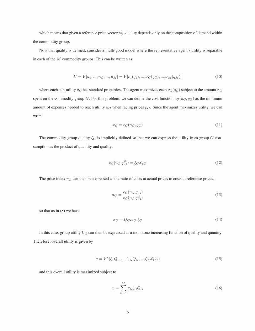
which means that given a reference price vector p0G, quality depends only on the composition of demand within
the commodity group.
Now that quality is defined, consider a multi-good model where the representative agent’s utility is separable
in each of theM commodity groups. This can be written as:
U = V [u1, ..., uG, ..., uM ] = V ['1(q1), ...,'G(qG), ...,'M (qM )] (10)
where each sub-utility uG has standard properties. The agent maximizes each 'G(qG) subject to the amount xG
spent on the commodity group G. For this problem, we can define the cost function cG(uG, qG) as the minimum
amount of expenses needed to reach utility uG when facing prices pG. Since the agent maximizes utility, we can
write
xG = cG(uG, qG) (11)
The commodity group quality &G is implicitly defined so that we can express the utility from group G con-
sumption as the product of quantity and quality,
cG(uG, p0G) = &G.QG (12)
The price index %G can then be expressed as the ratio of costs at actual prices to costs at reference prices,
%G =cG(uG, pG)
cG(uG, p0G)
(13)
so that as in (8) we have
xG = QG.%G.&G (14)
In this case, group utility UG can then be expressed as a monotone increasing function of quality and quantity.
Therefore, overall utility is given by
u = V "((1Q1, ...,( 1GQG, ...,(MQM ) (15)
and this overall utility is maximized subject to
x =M!
G=1
%G(GQG (16)
6
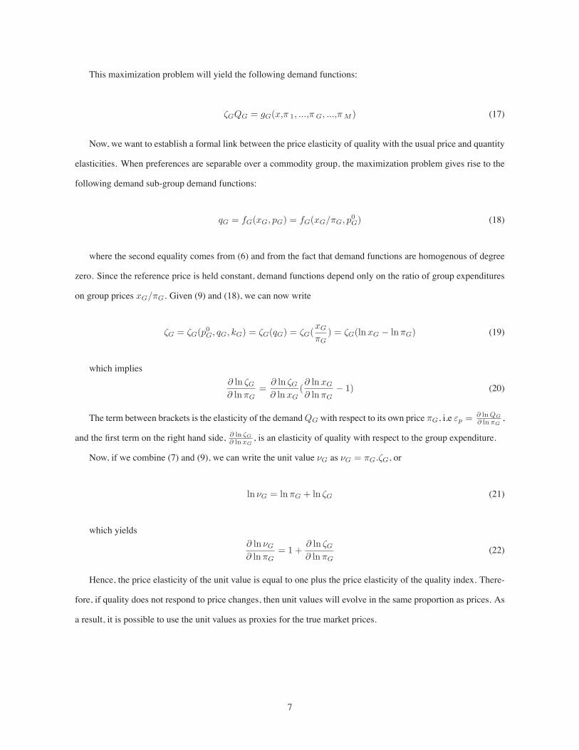
This maximization problem will yield the following demand functions:
(GQG = gG(x,% 1, ...,%G, ...,%M ) (17)
Now, we want to establish a formal link between the price elasticity of quality with the usual price and quantity
elasticities. When preferences are separable over a commodity group, the maximization problem gives rise to the
following demand sub-group demand functions:
qG = fG(xG, pG) = fG(xG/%G, p0G) (18)
where the second equality comes from (6) and from the fact that demand functions are homogenous of degree
zero. Since the reference price is held constant, demand functions depend only on the ratio of group expenditures
on group prices xG/%G. Given (9) and (18), we can now write
(G = (G(p0G, qG, kG) = (G(qG) = (G(
xG
%G) = (G(lnxG ! ln%G) (19)
which implies) ln (G
) ln%G=
) ln (G
) lnxG() lnxG
) ln%G! 1) (20)
The term between brackets is the elasticity of the demandQG with respect to its own price %G, i.e *p = ! ln QG
! ln "G,
and the first term on the right hand side, ! ln #G
! ln xG, is an elasticity of quality with respect to the group expenditure.
Now, if we combine (7) and (9), we can write the unit value 'G as 'G = %G.(G, or
ln 'G = ln%G + ln (G (21)
which yields) ln 'G
) ln%G= 1 +
) ln (G
) ln%G(22)
Hence, the price elasticity of the unit value is equal to one plus the price elasticity of the quality index. There-
fore, if quality does not respond to price changes, then unit values will evolve in the same proportion as prices. As
a result, it is possible to use the unit values as proxies for the true market prices.
7
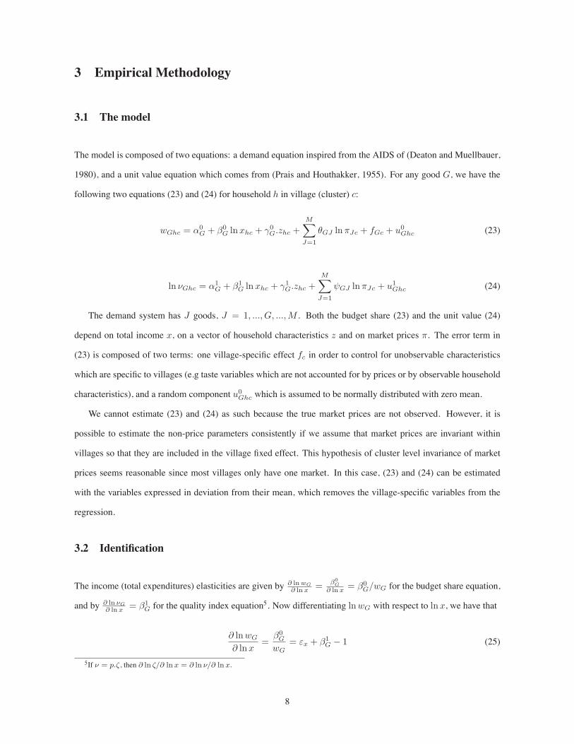
3 Empirical Methodology
3.1 The model
The model is composed of two equations: a demand equation inspired from the AIDS of (Deaton and Muellbauer,
1980), and a unit value equation which comes from (Prais and Houthakker, 1955). For any good G, we have the
following two equations (23) and (24) for household h in village (cluster) c:
wGhc = "0G + $0
G lnxhc + #0G.zhc +
M!
J=1
+GJ ln%Jc + fGc + u0Ghc (23)
ln 'Ghc = "1G + $1
G lnxhc + #1G.zhc +
M!
J=1
,GJ ln%Jc + u1Ghc (24)
The demand system has J goods, J = 1, ..., G, ...,M . Both the budget share (23) and the unit value (24)
depend on total income x, on a vector of household characteristics z and on market prices %. The error term in
(23) is composed of two terms: one village-specific effect fc in order to control for unobservable characteristics
which are specific to villages (e.g taste variables which are not accounted for by prices or by observable household
characteristics), and a random component u0Ghc which is assumed to be normally distributed with zero mean.
We cannot estimate (23) and (24) as such because the true market prices are not observed. However, it is
possible to estimate the non-price parameters consistently if we assume that market prices are invariant within
villages so that they are included in the village fixed effect. This hypothesis of cluster level invariance of market
prices seems reasonable since most villages only have one market. In this case, (23) and (24) can be estimated
with the variables expressed in deviation from their mean, which removes the village-specific variables from the
regression.
3.2 Identification
The income (total expenditures) elasticities are given by ! ln wG
! ln x= $0
G
! ln x= $0
G/wG for the budget share equation,
and by ! ln %G
! ln x= $1
G for the quality index equation5. Now differentiating lnwG with respect to lnx, we have that
) lnwG
) lnx=
$0G
wG= *x + $1
G ! 1 (25)
5If ! = p.", then # ln "/# ln x = # ln !/# ln x.
8

where *x is the income elasticity of demand6. Rearranging (25) gives us an analytical expression for the income
elasticity of demand based on the estimated parameters (for any good G):
*x ="
$0/w#
+ (1 ! $1) (26)
Similarly, differentiating lnwG with respect to ln% gives the direct and cross price elasticities for the budget
shares:
) lnwG/) ln% = *p + ,GJ = +GJ/wG (27)
Hence, for any good G:
*p = (+/w) ! , (28)
With this specification, the income and price elasticity of demand will vary according to the level of wG. We
will compute our estimates at mean budget shares (across households within villages).
We must now examine how to recover the coefficients of the price variables, namely , and +. To obtain ,, first
write the total expenditure elasticity of quality using the chain rule as
$1 = ) ln 'G/) lnx =) ln &G
) lnx=
) ln &G
) lnxG.) lnxG
) lnx(29)
The last term of the expression is the total expenditure elasticity of the group *x. If we combine (29) and (20),
we obtain) ln &G
) ln%G= $1.
*p
*x(30)
where *p is the price elasticity of demand. Moreover, since the elasticity of the unit value with respect to price
is given by (22), we find , as a function of the estimated parameters with
, = 1 + $1.*p
*x(31)
Now if we substitute (26) and (28) into (31) and rearrange, we obtain
, = 1 !$1(w ! +)
$0 + w(32)
, and + cannot be recovered directly from the data because market prices are not observed. However, we can6This is because w = (v.q)/x " ln w = ln v + ln q # ln x " # ln w/# ln x = # ln v/# ln x + # ln q/# ln x # 1
9
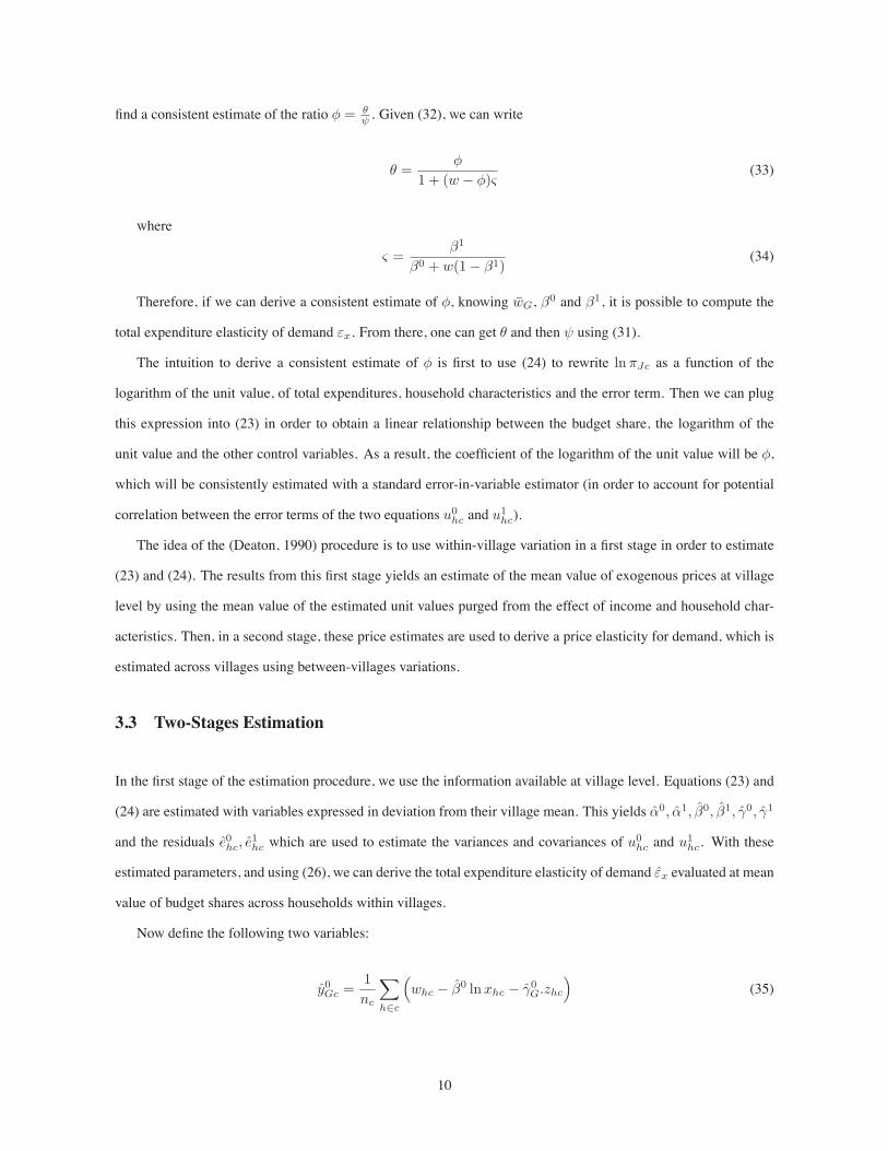
find a consistent estimate of the ratio - = &'. Given (32), we can write
+ =-
1 + (w ! -).(33)
where
. =$1
$0 + w(1 ! $1)(34)
Therefore, if we can derive a consistent estimate of -, knowing wG, $0 and $1, it is possible to compute the
total expenditure elasticity of demand *x. From there, one can get + and then , using (31).
The intuition to derive a consistent estimate of - is first to use (24) to rewrite ln%Jc as a function of the
logarithm of the unit value, of total expenditures, household characteristics and the error term. Then we can plug
this expression into (23) in order to obtain a linear relationship between the budget share, the logarithm of the
unit value and the other control variables. As a result, the coefficient of the logarithm of the unit value will be -,
which will be consistently estimated with a standard error-in-variable estimator (in order to account for potential
correlation between the error terms of the two equations u0hc and u1
hc).
The idea of the (Deaton, 1990) procedure is to use within-village variation in a first stage in order to estimate
(23) and (24). The results from this first stage yields an estimate of the mean value of exogenous prices at village
level by using the mean value of the estimated unit values purged from the effect of income and household char-
acteristics. Then, in a second stage, these price estimates are used to derive a price elasticity for demand, which is
estimated across villages using between-villages variations.
3.3 Two-Stages Estimation
In the first stage of the estimation procedure, we use the information available at village level. Equations (23) and
(24) are estimated with variables expressed in deviation from their village mean. This yields "0, "1, $0, $1, #0, #1
and the residuals e0hc, e
1hc which are used to estimate the variances and covariances of u0
hc and u1hc. With these
estimated parameters, and using (26), we can derive the total expenditure elasticity of demand *x evaluated at mean
value of budget shares across households within villages.
Now define the following two variables:
y0Gc =
1
nc
!
h#c
$
whc ! $0 lnxhc ! #0G.zhc
%
(35)
10

y1Gc =
1
n+c
!
h#c
$
ln vhc ! $1 lnxhc ! #1G.zhc
%
(36)
where nc is the number of households in village c, and n+c is the number of households who purchase good
G (and therefore who report unit values). These values, y0Gc and y1
Gc represent respectively the mean values
across households and within villages of the budget shares and unit values, purged from the effect of income and
observable household characteristics. In this setup, y1Gc is a proxy for mean exogenous prices at the village level.
As the number of observations increases, these values should converge to their true values y0Gc and y1
Gc which are
defined according to (23) and (24) as
y0Gc = "0
G +M!
j=1
+GJ ln%Jc + fGc + u0Gc (37)
y1Gc = "1
G +M!
j=1
,GJ ln%Jc + u1Gc (38)
Now, we can compute the matrices&
(the variance-covariance matrix of the budget shares, with elements
/GJ computed as in (39)), ! (variance-covariance matrix of the unit values, with elements !GJ computed as in
(40)), and 0 (variance-covariance matrix between budget shares and unit values, with elements !GJ computed as
in (41))7.
/GJ = (n ! C ! k)$1!
c
!
h#c
e0Ghc.e
0Jhc (39)
!GJ = (n+ ! C ! k)$1!
c
!
h#c
e1Ghc.e
1Jhc (40)
!GJ = (n+ ! C ! k)$1!
c
!
h#c
e0Ghc.e
1Jhc (41)
where n is the total number of observations, C is the number of villages and k is the number of explanatory
variables. n+ represents the number of households who declare buying the good G.
The second stage of the procedure uses between-clusters variations. We exploit the information obtained from
the variables at village-means (y0Gc for the budget shares and y1
Gc for the village prices) to derive a consistent
estimate of -. This is done by computing the variance-covariance matrix Q for the mean budget shares (with
elements qGJ estimated by (42)), S for the village prices (with elements sGJ estimated by (43)), and T for the7! and $ are assumed to be diagonal matrices with zero elements off-diagonal.
11

covariation between budget shares and prices (with elements tGJ estimated by (44)).
qGJ = cov(y0Gc, y
0Jc) (42)
sGJ = cov(y1Gc, y
1Jc) (43)
tGJ = cov(y0Gc, y
1Jc) (44)
At this stage, we can recover - by regressing the budget shares y0Gc on the village prices y1
c . Applying OLS
yields
-OLS =cov(y1
Gc, y1Jc)
var(y1c )
(45)
or, in the multivariate case,
BOLS = S$1.T (46)
This estimator must however be adjusted to account for potential measurement error bias, which would imply
correlation between the residuals u0Gc and u1
Gc in the first stage. Following (Griliches and Haussman, 1986), we
choose to implement the following error-in-variables estimator:
-EIV =cov(y1
Gc, y1Jc) ! 0/nc
var(y1c ) ! !/n+
c
(47)
or
BEIV =$
S ! !N$1+
%$1
.$
T ! 0N$1%
(48)
where N$1+ = C$1
&
c D(n+c )$1, and D(n+
c ) is a diagonal matrix which elements are nc.
The asymptotic formulae to derive the correct variance-covariance matrix for the estimated price elasticities
are hard to obtain. They must take into account the fact that the sample size vary from one good to another for
the estimation of the unit value equation. We follow an alternative approach which consists in bootstrapping the
second stage estimates of the price elasticities and computing the variance-covariance estimates of the parameters
from the boostrapped results.
12

4 Results
4.1 The Data
The data are drawn from the Vietnam Living Standard Survey (VLSS) conducted in 1998. The survey was de-
signed by stratified random sampling and is nationally representative. The primary sampling units are villages
(clusters). 370 villages have been surveyed, 108 of which are located in urban area. 6,000 households (about
28,000 individuals) have been interviewed.
Households are interviewed about their food and non-food consumption during the 12 months preceding the
survey. For all goods considered in the survey, households are asked whether or not they consume the good, and
in case of positive consumption, they are also asked about the expenditure value of the consumed good. This is
done both for market-purchased goods and for home-produced goods. Since we are interested in the variation of
total demand in response to price changes, the budget share for each good in the household consumption bundle
includes both market purchases and auto-consumption. However, the unit values are computed from purchased
goods only. Therefore, for a given good G, the sample size will differ whether we are considering equation (23)
or equation (24). The budget share equation includes all households belonging to village C, while the unit value
equation include only those who declare purchasing the good on the market. Table 1 describes the structure of the
survey and gives details on consumption and purchase patterns at village level for different categories of goods.
On average, 16 households are interviewed in each village, and about half of the interviewed households declare
consuming cigarettes.
We aggregate the 45 goods included in the consumption questionnaire into 13 broader categories: rice, staples,
meat, fish, fish sauce, vegetables, fruits, tofu, dairy products, alcohol, coffee, cigarettes, and other food expen-
ditures. The demand system is closed by adding a 14th good for all non-food expenditures. Table 2 shows the
importance of food expenditures in total budget across the seven administrative regions and across expenditure
quintile. In all regions, the importance of food expenditures in households total budget decreases as households
get richer. Table 3 presents the budget shares and the unit values for each selected goods. On average, a pack
of cigarettes costs 3.2 thousands Vietnam Dongs (VND). Looking at figure 2.a, prices are higher in the two main
cities regions (Hanoi in Red River Delta, and Ho Chi Minh City in Southeast). Besides, reflecting the fact that unit
values also reflect quality choices, richer households consume more expensive products (figure 2.c). Cigarettes
represent less than 3% of the budget in the country, and less than 2% in northern regions. Figure 1.a confirms
the impression that cigarette consumption prevails more in southern regions than in the North. In fact, water pipe
13
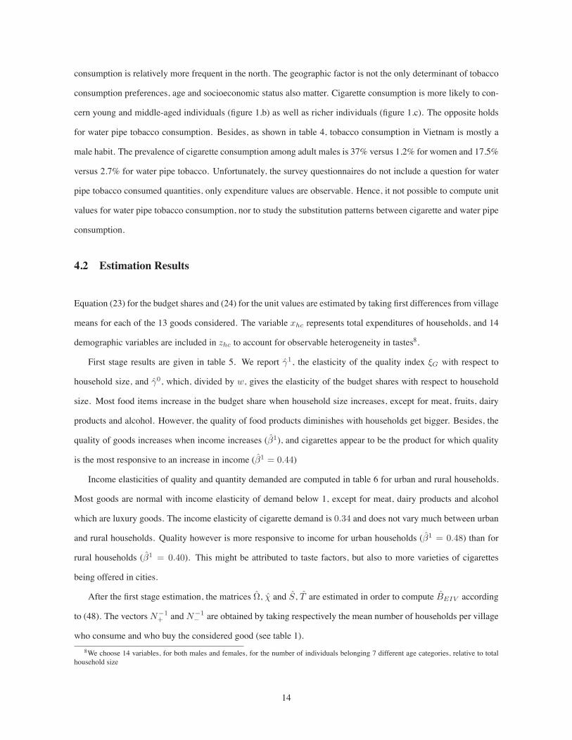
consumption is relatively more frequent in the north. The geographic factor is not the only determinant of tobacco
consumption preferences, age and socioeconomic status also matter. Cigarette consumption is more likely to con-
cern young and middle-aged individuals (figure 1.b) as well as richer individuals (figure 1.c). The opposite holds
for water pipe tobacco consumption. Besides, as shown in table 4, tobacco consumption in Vietnam is mostly a
male habit. The prevalence of cigarette consumption among adult males is 37% versus 1.2% for women and 17.5%
versus 2.7% for water pipe tobacco. Unfortunately, the survey questionnaires do not include a question for water
pipe tobacco consumed quantities, only expenditure values are observable. Hence, it not possible to compute unit
values for water pipe tobacco consumption, nor to study the substitution patterns between cigarette and water pipe
consumption.
4.2 Estimation Results
Equation (23) for the budget shares and (24) for the unit values are estimated by taking first differences from village
means for each of the 13 goods considered. The variable xhc represents total expenditures of households, and 14
demographic variables are included in zhc to account for observable heterogeneity in tastes8.
First stage results are given in table 5. We report #1, the elasticity of the quality index &G with respect to
household size, and #0, which, divided by w, gives the elasticity of the budget shares with respect to household
size. Most food items increase in the budget share when household size increases, except for meat, fruits, dairy
products and alcohol. However, the quality of food products diminishes with households get bigger. Besides, the
quality of goods increases when income increases ($1), and cigarettes appear to be the product for which quality
is the most responsive to an increase in income ($1 = 0.44)
Income elasticities of quality and quantity demanded are computed in table 6 for urban and rural households.
Most goods are normal with income elasticity of demand below 1, except for meat, dairy products and alcohol
which are luxury goods. The income elasticity of cigarette demand is 0.34 and does not vary much between urban
and rural households. Quality however is more responsive to income for urban households ($1 = 0.48) than for
rural households ($1 = 0.40). This might be attributed to taste factors, but also to more varieties of cigarettes
being offered in cities.
After the first stage estimation, the matrices !, 0 and S, T are estimated in order to compute BEIV according
to (48). The vectorsN$1+ andN$1
$ are obtained by taking respectively the mean number of households per village
who consume and who buy the considered good (see table 1).8We choose 14 variables, for both males and females, for the number of individuals belonging 7 different age categories, relative to total
household size
14

The Slutsky matrix + is estimated9 according to (33) and the results are reported in table 7. The variance of the
estimated parameters are bootstrapped, using 500 replications. The direct price elasticities lie on the diagonal of
the matrix, and most estimated direct elasticities are significant at 99% confidence level (95% for dairy products
and alcohol). The matrix is presented such that each entry gives the marginal change in demand for the column
good after and increase in price for the row good. Positive (negative) values of the entries indicate substitution
(complementarity) patterns in consumption. The estimated direct price elasticity of cigarette demand is !0.53.
This result is in the same order of magnitude as other estimates for developing countries, but based on different
methodologies (mostly based on time series data).
This suggest that tobacco taxation in Vietnam is likely to have a significant impact on cigarette consumption.
Middle aged wealthy men are the ones who would mostly bear the burden of such tax as this is the population
among which cigarette consumption is more prevalent. Moreover, since the estimated price elasticity is less than
one in absolute value, the introduction of cigarette taxation would also generate additional revenue for the govern-
ment budget. These conclusions must however be tempered for two reasons. The first one is that Vietnam share
boundaries with Cambodia, Laos and China and that increasing smuggling activity is also likely to be an outcome
of increased taxation of tobacco products in Vietnam. The second point is that unfortunately, because data on
quantities consumed were lacking in the survey, substitution patterns between water pipe tobacco and cigarette
consumption could not be analyzed.
5 Conclusion
We have used cross sectional household survey data with information on quantities and expenditures to derive
the spatial price elasticity of cigarette demand in Vietnam. In order to do so, we have followed Deaton (1990) to
specify an Almost Ideal Demand System and to combine this information with a model of simultaneous choice
for quantity and quality demanded. This allowed us to disentangle the influence of exogenous prices from quality
choices which are observationally combined in unit values. The main identification assumption of the procedure
is that prices are constant within villages, but they vary across villages because of weak market integration or high
transport costs.
The estimated price elasticity of cigarette demand is !0.53 and suggests that cigarette taxation should have a
significant impact on consumption while generating additional revenue for the government budget.9We did not impose a symmetry restriction on the estimation.
15
References
L. Christensen, D. Jorgensen, and L. Lau. Transcendental Logarithmic Utility Functions. American Economic
Review, 65:367–83, 1975.
A.S. Deaton. Quality, Quantity, and Spatial Variation of Prices. American Economic Review, 78:418–30, 1988.
A.S. Deaton. Price Elasticity From Survey Data: Extensions and Indonesian Results. Journal of Econometrics,
44:281–309, 1990.
A.S. Deaton. The Analysis of Household Survey: A Microeconometric Approach to Development Policy. The John
Hopkins University Press, Baltimore, 1997.
A.S. Deaton and F. Grimard. Demand Analysis for Tax Reform in Pakistan. LSMS Working Papers, World Bank,
85, 1992.
A.S. Deaton and J. Muellbauer. An Almost Ideal Demand System. American Economic Review, 70:312–26, 1980.
Z. Griliches and J.A. Haussman. Error-in-Variables in Panel Data. Journal of Econometrics, 31:93–118, 1986.
J. Prabhat and F. Chaloupka. Tobacco Control in Developing Countries. Oxford University Press, Oxford, 2000.
S.J. Prais and H.S. Houthakker. The Analysis of Family Budget. Cambridge University Press, Cambridge, 1955.
R. Stone. Linear Expenditure System and Demand Analysis: An Application to The Pattern of Brittish Demand.
Economic Journal, 64:511–27, 1954.
H. Theil. The Information Approach to Demand Analysis. Econometrica, 31:65–87, 1965.
WHO. Tobacco or Health: A Global Status Report. World Health Organization, Geneva, 1997.
16

Table 1. Number of Households Per Villages (Consuming or Buying)
Total Sample Urban Rural
Consume Purchase Consume Purchase Consume Purchase
Rice 16.5 11.2 16.2 15.4 16.6 9.5
Staples 15.1 14.6 15.4 15.3 15.0 14.3
Meat 16.3 16.1 16.0 16.0 16.4 16.2
Fish 16.2 14.9 16.0 15.8 16.3 14.6
Fish Sauce 15.9 15.3 16.0 15.6 15.9 15.2
Vegetables 16.3 15.3 16.2 16.0 16.4 14.9
Fruits 15.4 13.0 15.7 15.2 15.3 12.11
Tofu 13.0 12.9 14.2 14.2 12.5 12.3
Dairy 4.6 4.2 7.4 6.9 3.5 3.1
Alcohol 9.0 8.1 6.9 6.7 9.9 8.7
Coffee 12.0 11.0 11.3 10.7 12.4 11.0
Cigarettes 7.8 7.7 8.7 8.7 7.5 7.3
Other 16.4 16.4 16.2 16.2 16.5 16.5
# villages 370 108 262
Source: VLSS 1998
Table 2. Alimentary Part of Budget (%)
North. Red North South Cent. Southeast Mekong
Mount. River Cent. Cent. Highland (HCMC) River
Quintile 1 62.4 61.9 58.9 62.3 71.8 58.7 61.6
Quintile 2 57.5 57.8 58.4 58.1 59.5 58.9 57.0
Quintile 3 54.3 54.6 54.1 53.6 53.0 56.2 54.9
Quintile 4 50.0 50.9 48.6 49.5 49.0 52.3 50.4
Quintile 5 40.4 40.8 38.0 41.3 36.6 40.4 40.4
Source: VLSS 1998
17

Table 3a. Budget Shares by Commodity Groups and by Regions (%)
North. Red North South Cent. Southeast Mekong
Mount. River Cent. Cent. Highland (HCMC) River
Rice 25.70 19.71 22.62 18.95 26.26 11.42 19.05
Staples 2.58 2.06 2.54 2.54 1.86 1.54 1.04
Meat 8.70 8.65 6.88 5.80 8.24 6.71 7.57
Fish 2.79 3.69 5.20 5.79 4.94 4.42 6.55
Fish Sauce 0.53 0.72 1.00 0.98 0.69 0.53 0.71
Vegetables 1.60 1.66 1.53 2.39 1.96 1.90 2.02
Fruits 1.12 1.58 1.36 1.30 1.23 1.55 1.67
Tofu 1.02 1.01 0.62 0.48 0.48 0.57 0.36
Dairy 0.10 0.23 0.14 0.17 0.18 0.58 0.17
Alcohol 1.16 0.85 1.04 0.62 1.65 0.47 0.42
Coffee 0.78 0.89 1.04 0.51 0.53 0.57 0.41
Cigarettes 0.81 1.12 1.22 2.67 2.46 2.67 2.71
Other 6.54 9.15 7.57 9.58 7.20 13.14 9.05
# obs 859 1175 708 754 368 1023 112
Source: VLSS 1998
18

Table 3b. Unit Values by Commodity Groups and by Regions (TVND/qty unit)
North. Red North South Cent. Southeast Mekong
Mount. River Cent. Cent. Highland (HCMC) River
Rice 3.75 3.79 3.69 3.65 3.35 3.92 3.51
Staples 6.80 5.87 6.03 7.94 9.49 8.13 7.50
Meat 17.74 18.26 15.72 19.43 19.58 24.62 19.03
Fish 11.98 12.85 10.35 9.26 10.64 20.11 12.48
Fish Sauce 4.07 4.88 4.14 4.80 4.82 5.61 3.14
Vegetables 2.01 2.00 2.23 3.64 3.57 3.73 3.24
Fruits 4.21 5.04 4.12 4.25 4.16 5.40 5.05
Tofu 3.50 3.90 4.25 4.60 4.67 4.76 6.00
Dairy 19.57 21.28 20.02 20.69 18.61 23.01 19.20
Alcohol 4.61 5.24 6.02 5.56 4.14 7.43 4.12
Coffee 23.22 29.87 20.35 22.89 23.61 37.14 35.60
Cigarettes 2.06 3.03 2.37 2.83 1.95 4.91 3.03
Other 9.42 8.51 9.37 9.72 8.92 9.48 8.06
# obs 859 1175 708 754 368 1023 112
Source: VLSS 1998
19
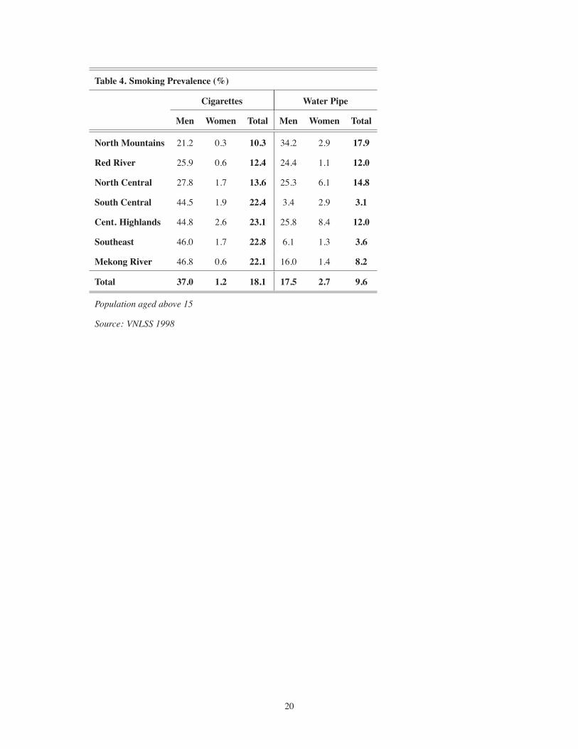
Table 4. Smoking Prevalence (%)
Cigarettes Water Pipe
Men Women Total Men Women Total
North Mountains 21.2 0.3 10.3 34.2 2.9 17.9
Red River 25.9 0.6 12.4 24.4 1.1 12.0
North Central 27.8 1.7 13.6 25.3 6.1 14.8
South Central 44.5 1.9 22.4 3.4 2.9 3.1
Cent. Highlands 44.8 2.6 23.1 25.8 8.4 12.0
Southeast 46.0 1.7 22.8 6.1 1.3 3.6
Mekong River 46.8 0.6 22.1 16.0 1.4 8.2
Total 37.0 1.2 18.1 17.5 2.7 9.6
Population aged above 15
Source: VNLSS 1998
20
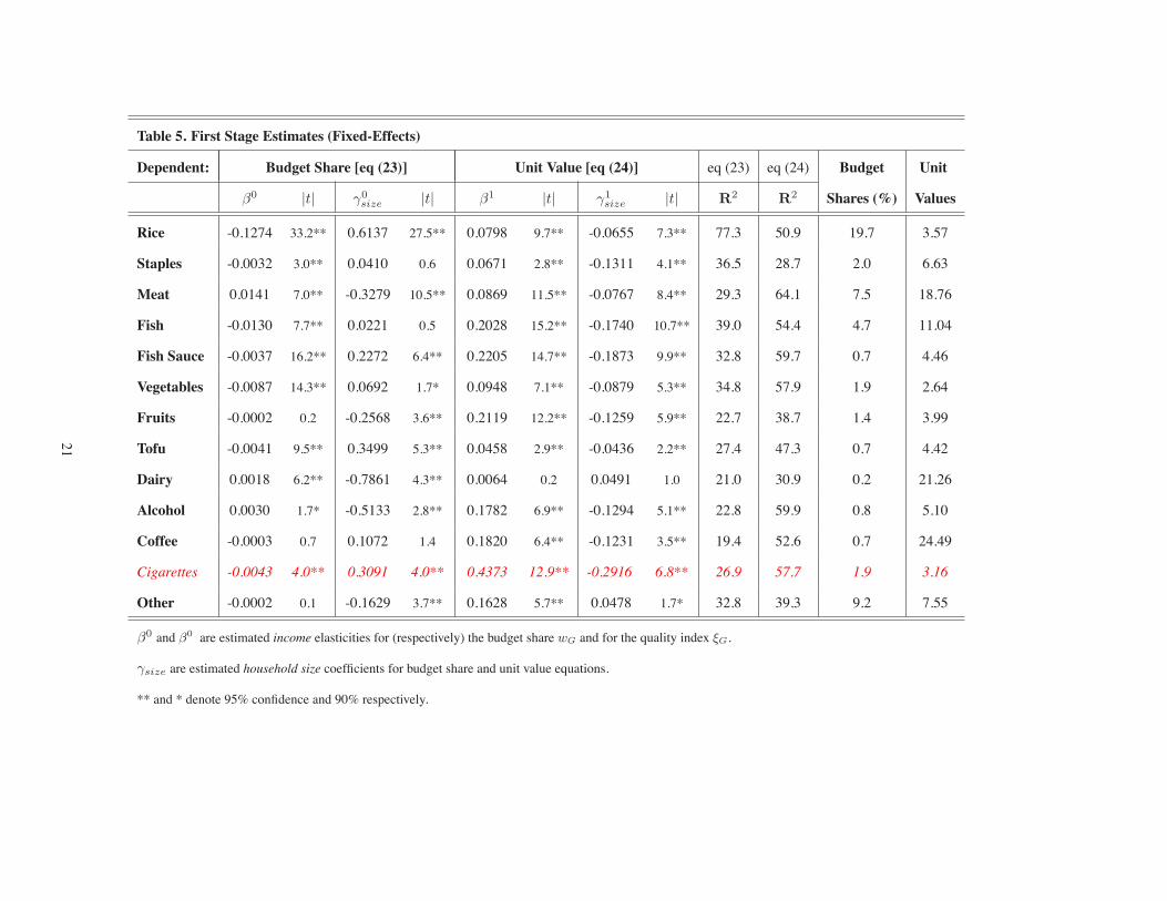
Table 5. First Stage Estimates (Fixed-Effects)
Dependent: Budget Share [eq (23)] Unit Value [eq (24)] eq (23) eq (24) Budget Unit
$0 |t| #0size |t| $1 |t| #1
size |t| R2 R2 Shares (%) Values
Rice -0.1274 33.2** 0.6137 27.5** 0.0798 9.7** -0.0655 7.3** 77.3 50.9 19.7 3.57
Staples -0.0032 3.0** 0.0410 0.6 0.0671 2.8** -0.1311 4.1** 36.5 28.7 2.0 6.63
Meat 0.0141 7.0** -0.3279 10.5** 0.0869 11.5** -0.0767 8.4** 29.3 64.1 7.5 18.76
Fish -0.0130 7.7** 0.0221 0.5 0.2028 15.2** -0.1740 10.7** 39.0 54.4 4.7 11.04
Fish Sauce -0.0037 16.2** 0.2272 6.4** 0.2205 14.7** -0.1873 9.9** 32.8 59.7 0.7 4.46
Vegetables -0.0087 14.3** 0.0692 1.7* 0.0948 7.1** -0.0879 5.3** 34.8 57.9 1.9 2.64
Fruits -0.0002 0.2 -0.2568 3.6** 0.2119 12.2** -0.1259 5.9** 22.7 38.7 1.4 3.99
Tofu -0.0041 9.5** 0.3499 5.3** 0.0458 2.9** -0.0436 2.2** 27.4 47.3 0.7 4.42
Dairy 0.0018 6.2** -0.7861 4.3** 0.0064 0.2 0.0491 1.0 21.0 30.9 0.2 21.26
Alcohol 0.0030 1.7* -0.5133 2.8** 0.1782 6.9** -0.1294 5.1** 22.8 59.9 0.8 5.10
Coffee -0.0003 0.7 0.1072 1.4 0.1820 6.4** -0.1231 3.5** 19.4 52.6 0.7 24.49
Cigarettes -0.0043 4.0** 0.3091 4.0** 0.4373 12.9** -0.2916 6.8** 26.9 57.7 1.9 3.16
Other -0.0002 0.1 -0.1629 3.7** 0.1628 5.7** 0.0478 1.7* 32.8 39.3 9.2 7.55
$0 and !0 are estimated income elasticities for (respectively) the budget share wG and for the quality index "G.
#size are estimated household size coefficients for budget share and unit value equations.
** and * denote 95% confidence and 90% respectively.
21
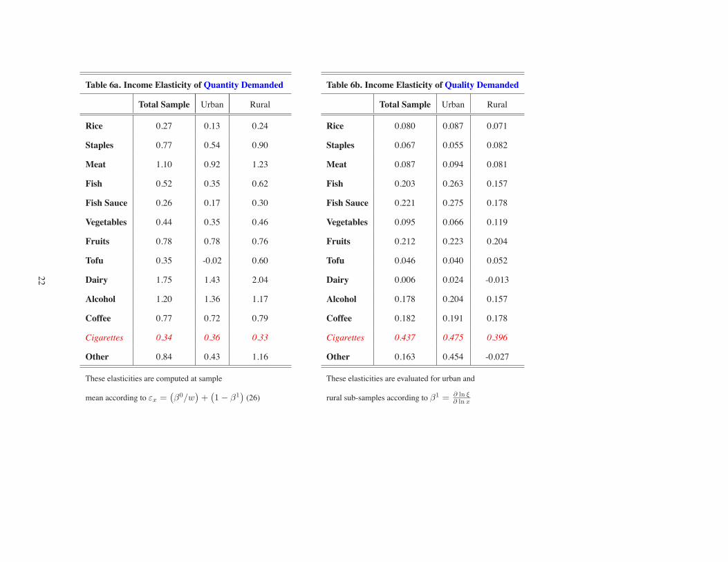
Table 6a. Income Elasticity of Quantity Demanded
Total Sample Urban Rural
Rice 0.27 0.13 0.24
Staples 0.77 0.54 0.90
Meat 1.10 0.92 1.23
Fish 0.52 0.35 0.62
Fish Sauce 0.26 0.17 0.30
Vegetables 0.44 0.35 0.46
Fruits 0.78 0.78 0.76
Tofu 0.35 -0.02 0.60
Dairy 1.75 1.43 2.04
Alcohol 1.20 1.36 1.17
Coffee 0.77 0.72 0.79
Cigarettes 0.34 0.36 0.33
Other 0.84 0.43 1.16
These elasticities are computed at sample
mean according to *x ="
$0/w#
+"
1 ! $1#
(26)
Table 6b. Income Elasticity of Quality Demanded
Total Sample Urban Rural
Rice 0.080 0.087 0.071
Staples 0.067 0.055 0.082
Meat 0.087 0.094 0.081
Fish 0.203 0.263 0.157
Fish Sauce 0.221 0.275 0.178
Vegetables 0.095 0.066 0.119
Fruits 0.212 0.223 0.204
Tofu 0.046 0.040 0.052
Dairy 0.006 0.024 -0.013
Alcohol 0.178 0.204 0.157
Coffee 0.182 0.191 0.178
Cigarettes 0.437 0.475 0.396
Other 0.163 0.454 -0.027
These elasticities are evaluated for urban and
rural sub-samples according to $1 = ! ln (! ln x
22

Table 7. Slutsky Substitution Matrix
Rice Staple Meat Fish Fish S. Veget. Fruits Tofu Dairy Alc. Coffee Cig.
Rice -0,38** 0,02 -0,12 -0,04 -0,02 -0,05 0,01 0,01 -0,07 0,03 0,02 -0,01
Staple -0,48 -0,86** -1,06* -0,03 0,26* 0,09 -0,13 0,03 0,05 0,30 -0,05 -0,01
Meat -0,27 -0,09 -0,96** 0,20** 0,05 -0,15 0,02 -0,06 0,09 -0,41** 0,02 0,01
Fish 0,35 -0,12 0,43 -0,82** -0,05 0,25* 0,01 0,26** -0,14 -0,15 -0,07 0,00
Fish Sauce -0,27 -0,12 -0,11 -0,14* -0,44** 0,14 -0,05 0,23** 0,09 0,18 -0,03 0,03
Vegetables 0,37 -0,17 0,26 0,01 0,03 -0,48** 0,06 0,04 0,14 0,00 0,03 -0,05
Fruits 0,46 -0,10 -0,15 0,13 -0,04 -0,08 -0,75** 0,09 -0,01 0,14 0,03 -0,04
Tofu -0,64 0,11 -0,32 0,28* 0,12 -0,52* 0,17 -1,17** 0,36 0,15 0,17* 0,01
Dairy 0,26 -0,16 1,67 0,35 0,13 -0,01 -0,18 0,24 -1,38* 0,42 0,07 -0,09
Alcohol -0,14 -0,10 -1,00* -0,25 0,04 -0,20 -0,09 -0,27 0,04 -0,63* -0,19 -0,12
Coffee -0,45 -0,32 -0,03 0,03 0,10 0,03 -0,03 0,17 0,32 -0,34 -0,98** 0,12
Cigarettes -0,02 0,00 0,23 -0,10 0,01 0,12 0,05 0,14 -0,06 0,26** 0,02 -0,53**
** and * denote respectively 99% and 95% confidence level (standard errors are bootstrapped )
The matrix entries give the marginal increase in demand for the good in column when the
price of the row commodity increases at the margin (own price elasticities are in bold)
23
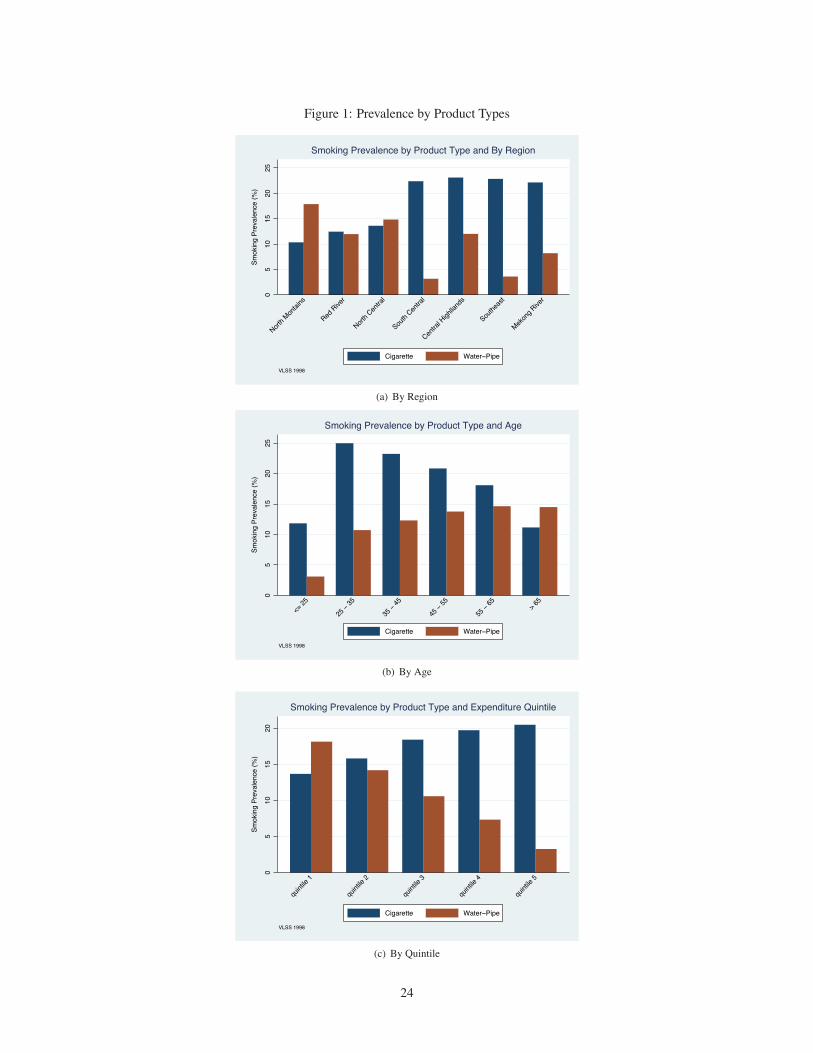
Figure 1: Prevalence by Product Types
05
1015
2025
Smok
ing
Prev
alen
ce (%
)
North M
ontai
ns
Red Rive
r
North C
entra
l
South
Centra
l
Centra
l High
llands
Southe
ast
Mekon
g Rive
r
VLSS 1998
Smoking Prevalence by Product Type and By Region
Cigarette Water−Pipe
(a) By Region
05
1015
2025
Smok
ing
Prev
alen
ce (%
)
<= 25
25 −
35
35 −
45
45 −
55
55 −
65 > 65
VLSS 1998
Smoking Prevalence by Product Type and Age
Cigarette Water−Pipe
(b) By Age
05
1015
20
Smok
ing
Prev
alen
ce (%
)
quint
ile 1
quint
ile 2
quint
ile 3
quint
ile 4
quint
ile 5
VLSS 1998
Smoking Prevalence by Product Type and Expenditure Quintile
Cigarette Water−Pipe
(c) By Quintile
24
Figure 2: Number of Cigarettes Smoked Per Day
05
1015
Num
ber O
f Cig
aret
tes
Smok
ed P
er D
ay P
er S
mok
er
North M
ounta
in
Red Rive
r
North C
entra
l
South
Centra
l
Centra
l High
land
Southe
ast
Mekon
g Rive
r
VLSS 1998
Number of Cigarettes Smoked by Region
(a) By Region
05
1015
Num
ber O
f Cig
aret
tes
Smok
ed P
er D
ay P
er S
mok
er
< 25
25 −
35
35 −
45
45 −
55
55 −
65 > 65
VLSS 1998
Number of Cigarettes Smoked by Age
(b) By Age
05
1015
Num
ber O
f Cig
aret
tes
Smok
ed P
er D
ay P
er S
mok
er
quint
ile 1
quint
ile 2
quint
ile 3
quint
ile 4
quint
ile 5
VLSS 1998
Number of Cigarettes Smoked by Expenditure Quintile
(c) By Quintile
25

Figure 3: Unit Values
01
23
45
Unit
Valu
e Fo
r 1 P
ack
(TVN
D)
North M
ounta
in
Red Rive
r
North C
entra
l
South
Centra
l
Centra
l High
land
Southe
ast
Mekon
g Rive
r
VLSS 1998
Cigarette Unit Values by Region
(a) By Region
01
23
4
Unit
Valu
e Fo
r 1 P
ack
(TVN
D)
< 25
25 −
35
35 −
45
45 −
55
55 −
65 > 65
VLSS 1998
Cigarette Unit Values by Age
(b) By Age
01
23
45
Unit
Valu
e Fo
r 1 P
ack
(TVN
D)
quint
ile 1
quint
ile 2
quint
ile 3
quint
ile 4
quint
ile 5
VLSS 1998
Cigarette Unit Values by Expenditure Quintile
(c) By Quintile
26


