NAVAL
POSTGRADUATE SCHOOL
MONTEREY, CALIFORNIA
THESIS
Approved for public release; distribution is unlimited
CONFLICT RESOLUTION AND OPTIMIZATION OF MULTIPLE-SATELLITE SYSTEMS (CROMSAT)
by
Brett N. Laboo
June 2007
Thesis Advisor: R.F. Dell Co-Advisor: I.M. Ross Second Reader: W. Kang

THIS PAGE INTENTIONALLY LEFT BLANK
i
REPORT DOCUMENTATION PAGE Form Approved OMB No. 0704-0188 Public reporting burden for this collection of information is estimated to average 1 hour per response, including the time for reviewing instruction, searching existing data sources, gathering and maintaining the data needed, and completing and reviewing the collection of information. Send comments regarding this burden estimate or any other aspect of this collection of information, including suggestions for reducing this burden, to Washington headquarters Services, Directorate for Information Operations and Reports, 1215 Jefferson Davis Highway, Suite 1204, Arlington, VA 22202-4302, and to the Office of Management and Budget, Paperwork Reduction Project (0704-0188) Washington DC 20503. 1. AGENCY USE ONLY (Leave blank)
2. REPORT DATE June 2007
3. REPORT TYPE AND DATES COVERED Master’s Thesis
4. TITLE AND SUBTITLE: Conflict Resolution and Optimization of Multiple-Satellite Systems (CROMSAT) 6. AUTHOR(S) Brett N. Laboo
5. FUNDING NUMBERS
7. PERFORMING ORGANIZATION NAME(S) AND ADDRESS(ES): Naval Postgraduate School Monterey, CA 93943-5000
8. PERFORMING ORGANIZATION REPORT NUMBER:
9. SPONSORING /MONITORING AGENCY NAME(S) AND ADDRESS(ES) Nil
10. SPONSORING/MONITORING AGENCY REPORT NUMBER
11. SUPPLEMENTARY NOTES: The views expressed in this thesis are those of the author and do not reflect the official policy or position of the Department of Defense or the U.S. Government. 12a. DISTRIBUTION / AVAILABILITY STATEMENT: Approved for public release; distribution is unlimited
12b. DISTRIBUTION CODE: A
13. ABSTRACT (maximum 200 words) This thesis produces models of satellite constellations using finite state automata (FSA) or finite automata
(FA) and optimizes the sequence of targets for two missions. Two simplified FSA models of satellite constellations with one ground control station (GCS) are developed. The first model is of a single spacecraft and the second includes two spacecraft. Based upon the language, states, and state transitions of each model, the author transforms the FA into a network and enumerates the shortest paths for indicative lists of meta-tasks from each model. The first model is provisionally implemented in MATLAB. The author finds two separate optimal target selection sequences for randomly generated sample target sets using commercial off-the-shelf optimization software. Although stochastically fabricated, the sample target sets reflect valid scenarios for a satellite imagery mission. The first sequence, a traveling salesman problem, minimizes the time required for processing all targets given a multiple orbit mission. For a representative sample target set, this is 2.34 orbits. The second sequence, a prize collecting traveling salesman problem, maximizes the number of targets processed given a dual orbit mission. For the same sample target set, two orbits permit the processing of seven targets.
15. NUMBER OF PAGES
86
14. SUBJECT TERMS Satellite, Optimization, Finite Automata, Finite State Automata, Finite State Machine, Traveling Salesman Problem, Prize Collecting Traveling Salesman Problem
16. PRICE CODE
17. SECURITY CLASSIFICATION OF REPORT
Unclassified
18. SECURITY CLASSIFICATION OF THIS PAGE
Unclassified
19. SECURITY CLASSIFICATION OF ABSTRACT
Unclassified
20. LIMITATION OF ABSTRACT
UL NSN 7540-01-280-5500 Standard Form 298 (Rev. 2-89) Prescribed by ANSI Std. 239-18

ii
THIS PAGE INTENTIONALLY LEFT BLANK
iii
Approved for public release; distribution is unlimited
CONFLICT RESOLUTION AND OPTIMIZATION OF MULTIPLE-SATELLITE SYSTEMS (CROMSAT)
Brett N. Laboo
Major, Australian Army B.Sc., University of New South Wales
(Australian Defence Force Academy), 1994
Submitted in partial fulfillment of the requirements for the degree of
MASTER OF SCIENCE IN OPERATIONS RESEARCH
from the
NAVAL POSTGRADUATE SCHOOL June 2007
Author: Brett N. Laboo
Approved by: Prof. R.F. Dell Thesis Advisor
Prof. I.M. Ross Co-Advisor
Prof. W. Kang Second Reader
James N. Eagle Chairman, Department of Operations Research

iv
THIS PAGE INTENTIONALLY LEFT BLANK
v
ABSTRACT
This thesis produces models of satellite constellations using finite state
automata (FSA) or finite automata (FA) and optimizes the sequence of targets for
two missions. Two simplified FSA models of satellite constellations with one
ground control station (GCS) are developed. The first model is of a single
spacecraft and the second includes two spacecraft. Based upon the language,
states, and state transitions of each model, the author transforms the FA into a
network and enumerates the shortest paths for indicative lists of meta-tasks from
each model. The first model is provisionally implemented in MATLAB. The
author finds two separate optimal target selection sequences for randomly
generated sample target sets using commercial off-the-shelf optimization
software. Although stochastically fabricated, the sample target sets reflect valid
scenarios for a satellite imagery mission. The first sequence, a traveling
salesman problem, minimizes the time required for processing all targets given a
multiple orbit mission. For a representative sample target set, this is 2.34 orbits.
The second sequence, a prize collecting traveling salesman problem, maximizes
the number of targets processed given a dual orbit mission. For the same
sample target set, two orbits permit the processing of seven targets.

vi
THIS PAGE INTENTIONALLY LEFT BLANK
vii
TABLE OF CONTENTS
I. INTRODUCTION............................................................................................. 1 A. BACKGROUND ................................................................................... 1 B. DIRECTION OF RESEARCH............................................................... 2
II. FUNDAMENTALS .......................................................................................... 3 A. OUTLINE.............................................................................................. 3 B. DISTRIBUTED SPACECRAFT SYSTEMS (DSS) ............................... 3
1. Terrestrial Concerns................................................................ 3 a. Ground Control Station (GCS) ..................................... 4 b. Targets ........................................................................... 4
2. Vehicular Issues ...................................................................... 4 a. Design & Purpose ......................................................... 5 b. Tasks, Meta-tasks and Missions.................................. 5 c. Launch ........................................................................... 5 d. Orbits ............................................................................. 6 e. Lifetimes and Reliability ............................................... 7
3. Operating Environment........................................................... 8 a. Earth Related Effects .................................................... 8 b. Helio Effects .................................................................. 9
4. Stochastic Markovian Analysis of Inoperability.................... 9 C. FINITE AUTOMATA (FA) .................................................................... 9
1. Types of Finite Automata (FA)................................................ 9 2. Definition of FA ...................................................................... 10
a. Transition Diagram ..................................................... 10 b. Languages and Grammars......................................... 11 c. Symbolic Formulation and Description of an FA ..... 11
3. Transition Function ............................................................... 12 4. Alphabets ............................................................................... 13
a. Alphabet Elements...................................................... 13 b. Contribution to Network Formulations ..................... 14
5. Languages and Grammars.................................................... 14 6. Language Similarities............................................................ 16 7. Non-deterministic Finite Automata (NFA)............................ 16 8. Amalgamation of FA.............................................................. 16 9. Reduction and Equivalence.................................................. 17
D. OPTIMIZATION MODELS ................................................................. 17 1. Network Path Enumeration................................................... 17 2. Traveling Salesman Problem (TSP) ..................................... 18 3. Prize Collecting Traveling Salesman Problem (PCTSP)..... 18
E. RESEARCH QUESTIONS ................................................................. 18 1. Specific Research Questions ............................................... 18 2. Potential Research Extensions ............................................ 19
viii
III. THE MODELS............................................................................................... 21 A. MODEL DISCUSSION ....................................................................... 21 B. DSS CHARACTERISTICS................................................................. 21
1. Orbit Assumptions ................................................................ 21 2. Ground Control Station (GCS).............................................. 22 3. Communications.................................................................... 22 4. Transition Probability Matrix ................................................ 22
C. SINGLE SPACECRAFT FA............................................................... 24 1. States (Q)................................................................................ 24 2. Alphabet (∑ ) .......................................................................... 25 3. Start State (qo)........................................................................ 26 4. Final States (F) ....................................................................... 26 5. Transition Function (δ).......................................................... 26
D. DUAL SPACECRAFT FA .................................................................. 27 1. States (Q)................................................................................ 28 2. Alphabet (∑ ) .......................................................................... 29 3. Start State (qo)........................................................................ 31 4. Final States (F) ....................................................................... 31 5. Transition Function (δ).......................................................... 31
E. LANGUAGE OF THE MODELS – L(M) ............................................. 32 1. Single Spacecraft L(M) Construction................................... 32
a. Tasks............................................................................ 32 b. Meta-tasks ................................................................... 32
2. Dual spacecraft L(M) Construction ...................................... 33 a. Tasks............................................................................ 33 b. Meta-tasks ................................................................... 34
F. GRAPHICAL REPRESENTATIONS.................................................. 38 G. MATLAB ............................................................................................ 38
IV. TARGETRY OPTIMIZATION........................................................................ 39 A. TARGETRY MODEL.......................................................................... 39
1. Generation of Target Data..................................................... 39 2. Data Preparation .................................................................... 41
B. FORMULATIONS............................................................................... 42 1. TSP Formulation .................................................................... 42 2. PCTSP Formulation ............................................................... 43
C. RESULTS........................................................................................... 45 1. TSP Results............................................................................ 45 2. PCTSP Results....................................................................... 45 3. Discussion.............................................................................. 45
V. CONCLUSION AND RECOMMENDATIONS............................................... 47 A. CONCLUSION ................................................................................... 47 B. RECOMMENDATIONS...................................................................... 47
1. Graphical Representations ................................................... 48 2. More Spacecraft in the Model ............................................... 48
ix
3. NFA ......................................................................................... 48 4. PDA ......................................................................................... 49 5. Integer Linear Programming (ILP) Relationship to FA ....... 49
APPENDIX A. Dual Spacecraft FA – Transition Function (δ) ..................... 51
APPENDIX B. MATLAB Code for Single Spacecraft FA ............................. 55
LIST OF REFERENCES.......................................................................................... 57
INITIAL DISTRIBUTION LIST ................................................................................. 63

x
THIS PAGE INTENTIONALLY LEFT BLANK
xi
LIST OF FIGURES
Figure 1. Indicative Satellite Track, with GCS & its LEO Black-out Region ......... 7 Figure 2. Example of a Graphical Transition Diagram (After Hennie, 1968;
Hopcroft & Ullman, 1979) ................................................................... 11 Figure 3. Map of the Earth with Target Locations, Dwell Periods, and
Blackout Region ................................................................................. 40

xii
THIS PAGE INTENTIONALLY LEFT BLANK
xiii
LIST OF TABLES
Table 1. Example Transition Function (After Hennie, 1968; Hopcroft & Ullman, 1979) ..................................................................................... 13
Table 2. Relationships between FA Components, Logical Machine & Network Concepts, (After Hopcroft & Ullman, 1979) .......................... 16
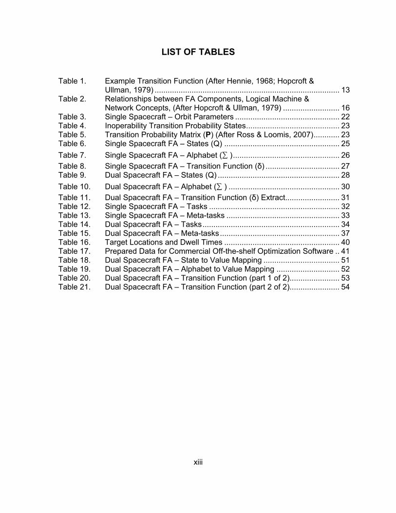
Table 3. Single Spacecraft – Orbit Parameters ................................................ 22 Table 4. Inoperability Transition Probability States........................................... 23 Table 5. Transition Probability Matrix (P) (After Ross & Loomis, 2007)............ 23 Table 6. Single Spacecraft FA – States (Q) ..................................................... 25 Table 7. Single Spacecraft FA – Alphabet (∑ )................................................. 26 Table 8. Single Spacecraft FA – Transition Function (δ) .................................. 27 Table 9. Dual Spacecraft FA – States (Q) ........................................................ 28 Table 10. Dual Spacecraft FA – Alphabet (∑ ) ................................................... 30 Table 11. Dual Spacecraft FA – Transition Function (δ) Extract......................... 31 Table 12. Single Spacecraft FA – Tasks ............................................................ 32 Table 13. Single Spacecraft FA – Meta-tasks .................................................... 33 Table 14. Dual Spacecraft FA – Tasks............................................................... 34 Table 15. Dual Spacecraft FA – Meta-tasks....................................................... 37 Table 16. Target Locations and Dwell Times ..................................................... 40 Table 17. Prepared Data for Commercial Off-the-shelf Optimization Software .. 41 Table 18. Dual Spacecraft FA – State to Value Mapping ................................... 51 Table 19. Dual Spacecraft FA – Alphabet to Value Mapping ............................. 52 Table 20. Dual Spacecraft FA – Transition Function (part 1 of 2)....................... 53 Table 21. Dual Spacecraft FA – Transition Function (part 2 of 2)....................... 54

xiv
THIS PAGE INTENTIONALLY LEFT BLANK
xv
ACKNOWLEDGMENTS
First and foremost, I acknowledge the blessings and divine providence of
Almighty God in the processes and events that have led to this thesis.
Next, I wish to thank my loving, devoted and understanding family. My
fascinating and wonderful ladies have endured much time apart from me as I
attempted to balance the demands of my time and efforts.
Obviously, this manuscript would not be anywhere as good as it is unless
there was clear and direct input and guidance from the Naval Postgraduate
School faculty and staff. Predominant among this distinguished cadre of
academics is my thesis team: my advisor, Prof. Rob Dell; my co-advisor,
Prof. Mike Ross; and my second reader Prof. Wei Kang. Gentlemen, thank you
all for your dedication, guidance and inspiration. Beyond this team, I am very
grateful for the assistance, contributions, suggestions and advice so graciously
provided by many others. In no particular order, I express my gratitude to the
late CAPT Starr King (USN), Prof. Bill Gragg, Prof. Arnie Buss, Prof. Hal
Fredricksen, Mr. Bard Mansager, Prof. Chris Darken, Prof. Dennis Volpano,
Mr. Bob Broadston, Dr. Pooya Sekhavat, Dr. Paul Sanchez, Prof. Bret Michael,
Prof. Cliff Whitcomb, Prof. Alan Ross, Prof. Hersch Loomis Jr., Mr. John Horning
and Mr. Joe Welch.
Finally, I take this opportunity to thank my peers; you all know who you
are. I have truly appreciated your friendship, support and encouragement during
our time at the Naval Postgraduate School. In the extremely unlikely event that
any of you should you ever actually need to use this thesis in any of your future
endeavors, I trust that by just reading these acknowledgements, it will conjure
penchant memories of our initial foray into the field of operations research at the
graduate level courtesy of the United States Navy.

xvi
THIS PAGE INTENTIONALLY LEFT BLANK
xvii
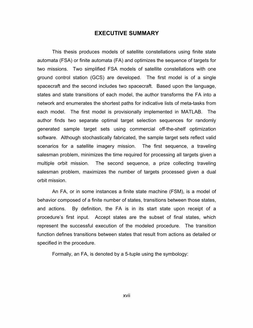
EXECUTIVE SUMMARY
This thesis produces models of satellite constellations using finite state
automata (FSA) or finite automata (FA) and optimizes the sequence of targets for
two missions. Two simplified FSA models of satellite constellations with one
ground control station (GCS) are developed. The first model is of a single
spacecraft and the second includes two spacecraft. Based upon the language,
states and state transitions of each model, the author transforms the FA into a
network and enumerates the shortest paths for indicative lists of meta-tasks from
each model. The first model is provisionally implemented in MATLAB. The
author finds two separate optimal target selection sequences for randomly
generated sample target sets using commercial off-the-shelf optimization
software. Although stochastically fabricated, the sample target sets reflect valid
scenarios for a satellite imagery mission. The first sequence, a traveling
salesman problem, minimizes the time required for processing all targets given a
multiple orbit mission. The second sequence, a prize collecting traveling
salesman problem, maximizes the number of targets processed given a dual
orbit mission.
An FA, or in some instances a finite state machine (FSM), is a model of
behavior composed of a finite number of states, transitions between those states,
and actions. By definition, the FA is in its start state upon receipt of a
procedure’s first input. Accept states are the subset of final states, which
represent the successful execution of the modeled procedure. The transition
function defines transitions between states that result from actions as detailed or
specified in the procedure.
Formally, an FA, is denoted by a 5-tuple using the symbology:
xviii
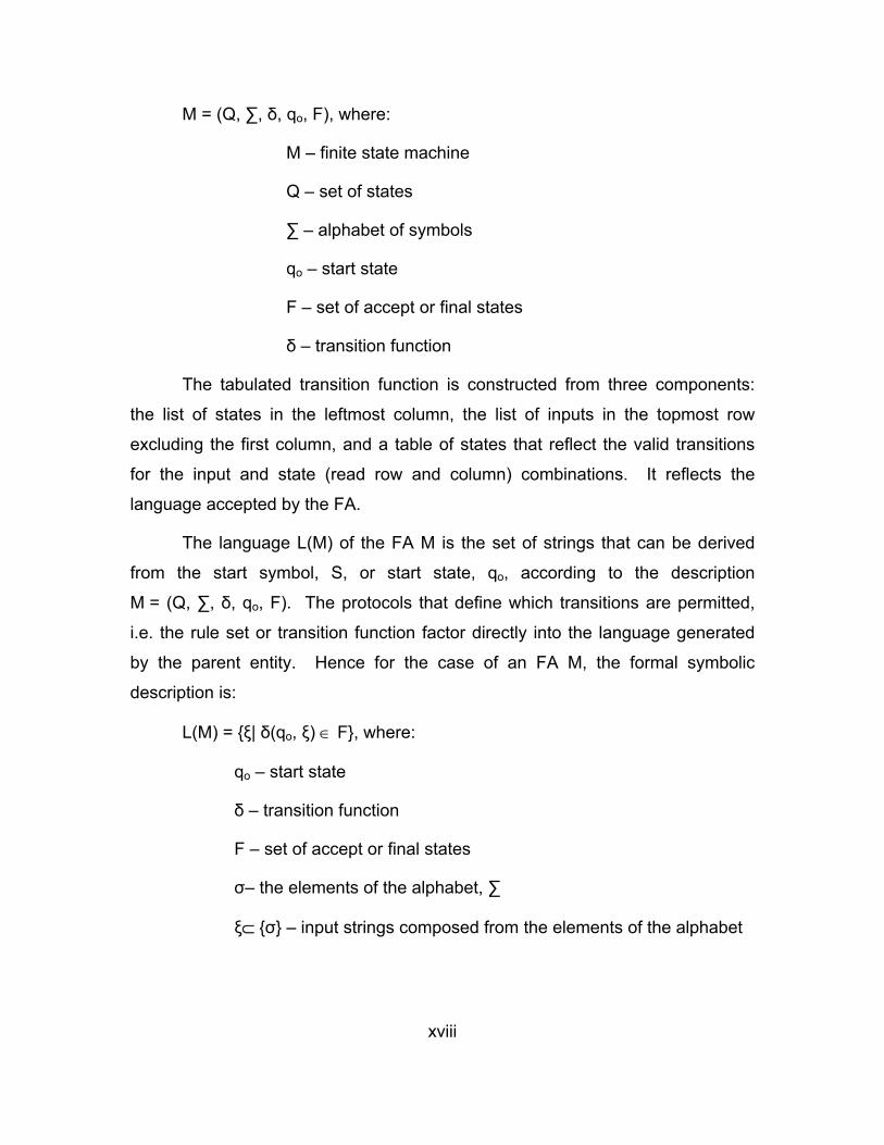
M = (Q, ∑, δ, qo, F), where:
M – finite state machine
Q – set of states
∑ – alphabet of symbols
qo – start state
F – set of accept or final states
δ – transition function
The tabulated transition function is constructed from three components:
the list of states in the leftmost column, the list of inputs in the topmost row
excluding the first column, and a table of states that reflect the valid transitions
for the input and state (read row and column) combinations. It reflects the
language accepted by the FA.
The language L(M) of the FA M is the set of strings that can be derived
from the start symbol, S, or start state, qo, according to the description
M = (Q, ∑, δ, qo, F). The protocols that define which transitions are permitted,
i.e. the rule set or transition function factor directly into the language generated
by the parent entity. Hence for the case of an FA M, the formal symbolic
description is:
L(M) = {ξ| δ(qo, ξ) ∈ F}, where:
qo – start state
δ – transition function
F – set of accept or final states
σ– the elements of the alphabet, ∑
ξ⊂ {σ} – input strings composed from the elements of the alphabet

xix
The author randomly generates eight target locations with corresponding
dwell times. For test instances, the traveling salesmen problem and the prize
collecting traveling salesmen problem each solve in less than one second using
commercial off-the-shelf software.

xx
THIS PAGE INTENTIONALLY LEFT BLANK
1
I. INTRODUCTION
This thesis produces models of satellite constellations using finite state
automata (FSA) or finite automata (FA) and optimizes the sequence of targets for
two missions. Two simplified FSA models of satellite constellations with one
ground control station (GCS) are developed. The first model is of a single
spacecraft and the second includes spacecraft. Based upon the language,
states and state transitions of each model, the author transforms the FA into a
network and enumerates the shortest paths for indicative lists of meta-tasks from
each model. The first model is provisionally implemented in MATLAB (MATLAB,
2007). The author finds two separate optimal target selection sequences. The
first, a traveling salesman problem, minimizes the time required for processing all
targets given a multiple orbit mission. The second, a prize collecting traveling
salesman problem, maximizes the number of targets processed given a dual
orbit mission.
A. BACKGROUND
Satellite systems have been in orbit since the successful launch of
Sputnik I on October 4, 1957. The complexity of the platforms and ground
controls stations (GCS) has increased and expanded considerably since then.
Commensurately the tasking has also developed. In terms of GCS personnel,
the initial concept of a large team of operators allocated to a single spacecraft
has now morphed into a distinctly contrasting situation where a multiple satellite
system is now controlled/co-coordinated by a single operator or a very small
team (Sekhavat, 2007). Given the adjustments of the workforce and the general
increase in demand for satellite imagery products, the tasking of satellites or
multiple satellite systems has become more complicated (Department of the
Army, 2005 & 2006). As various related technologies are further honed and
developed, the requirement for better management of the resource becomes
even more imperative (Ross I.M., 2006).
2
Thus, a method for examining the tasking of multiple satellite systems
aimed at resolving scheduling conflicts and optimizing both the task duration and
the spacecraft lifetimes should provide insight into potential cost savings and
improvements in the overall operation of the system.
B. DIRECTION OF RESEARCH
Potential future satellite systems will require greater distributed
functionality for cooperative execution of meta-tasks. A meta-task for a system
of satellites is analogous to a reconnaissance mission for ground troops. That is,
clearly specified with a standardized but concise vocabulary; for example,
“measure the distance to an approaching object" or “take pictures over 3° 07' S
latitude, 152° 38' E longitude.” Conflict resolution and optimization of the
scheduling and tasking of multiple satellites requires the identification of the
appropriate system components (i.e., satellites) that yield the most suitable
outcome. The optimal allocation of tasks is a considerable undertaking. The
problem is well-known to be NP-hard (Cassandras & Lafortune, 1999).
There are various extant models, methods and procedures for the analysis
of a satellite system. However, the author did not find the application of finite
state machines or finite state automata for generating the models, methods and
procedures for a satellite system as presented in this thesis. Finite state
machines or automata are used extensively in the computer science, digital
communications and electronic engineering fields (Cobleigh et al., 2002; Hennie,
1968). Employment beyond these fields has expanded since, but there remains
an apparent dearth of universal appeal of finite automata for many applications.
3
II. FUNDAMENTALS
A. OUTLINE
In order to achieve the aim of this undertaking, the author considers three
primary topics: space systems, finite automata (FA) and optimization models.
Space systems is an expansive field and thus the author focuses directly at the
specific problem under consideration. Where appropriate, the author made
simplifications to prevent the degeneration of this problem into the pits of
intractability. In addition, FA needs explanation and clarification in order to
establish the foundational concepts upon which the models are constructed and
where further research may be explored. Finally, the optimization models merit
discussion too. Then, with the essential groundwork covered, the author
specifies the particular research questions.
B. DISTRIBUTED SPACECRAFT SYSTEMS (DSS)
When considering the DSS it is necessary to clarify some of the specifics
as they apply to this problem. Space systems are very detailed and have a vast
array of constituent elements (Pisacane, 1994 & 2005). Grouping these into
three primary fields, namely terrestrial concerns, vehicular issues and the
operating environment, simplifies the discussion, permits a useful delineation
between topics and provides focus on the essential elements without loss of
generality.
1. Terrestrial Concerns
Terrestrial concerns are those matters which affect the construction of the
model from an earthbound perspective. In particular, there are two primary
concerns: the ground control station (GCS) and targets.
4
a. Ground Control Station (GCS)
In a DSS, the GCS plays a pivotal role. It is the central point
through which all communications are transmitted to and received from the DSS.
It monitors the status of each spacecraft in the DSS, either directly or remotely,
and as the name suggests, it is the focal point of control of the DSS. The GCS
determines orbit adjustments or realignments and transmits them to the relevant
spacecraft. The GCS may also provide the facilities for initial processing of any
imagery or data collection products. Additionally, the GCS may also conduct the
assignment and scheduling of spacecraft to targets along with the production of
the necessary telemetry and commands. For individual satellites, there are
different blackout regions for respective GCSs. These blackout regions are
predominantly a function of GCS location and orbit.
b. Targets
Targetry is a function of the payload. Payloads designed for
communications relay, interception and/or monitoring are used for relevant
exchanges. Whereas, in the case of a DSS in which the primary payload is for
imagery, the tasking is more focused on pictorial or graphical observations and
subsequent physical characteristic quantification. Designating targets with the
conventional longitude and latitude referencing system provides an inherent
baseline to Greenwich Mean Time (GMT).
2. Vehicular Issues
Referring to each spacecraft of a satellite system as a vehicle permits the
use of a commonly understood vernacular. Vehicular issues can be classified
into five distinct categories: design and purpose, tasks, launch, orbits and
lifetimes and reliabilities.
5
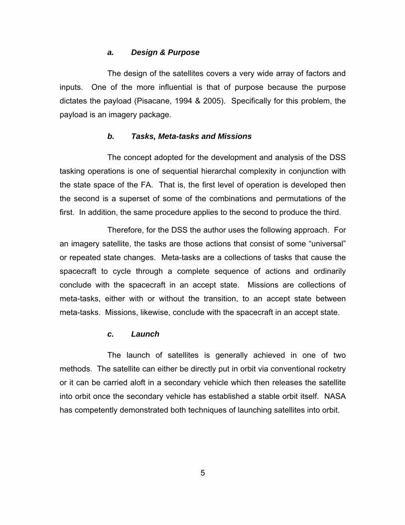
a. Design & Purpose
The design of the satellites covers a very wide array of factors and
inputs. One of the more influential is that of purpose because the purpose
dictates the payload (Pisacane, 1994 & 2005). Specifically for this problem, the
payload is an imagery package.
b. Tasks, Meta-tasks and Missions
The concept adopted for the development and analysis of the DSS
tasking operations is one of sequential hierarchal complexity in conjunction with
the state space of the FA. That is, the first level of operation is developed then
the second is a superset of some of the combinations and permutations of the
first. In addition, the same procedure applies to the second to produce the third.
Therefore, for the DSS the author uses the following approach. For
an imagery satellite, the tasks are those actions that consist of some “universal”
or repeated state changes. Meta-tasks are a collections of tasks that cause the
spacecraft to cycle through a complete sequence of actions and ordinarily
conclude with the spacecraft in an accept state. Missions are collections of
meta-tasks, either with or without the transition, to an accept state between
meta-tasks. Missions, likewise, conclude with the spacecraft in an accept state.
c. Launch
The launch of satellites is generally achieved in one of two
methods. The satellite can either be directly put in orbit via conventional rocketry
or it can be carried aloft in a secondary vehicle which then releases the satellite
into orbit once the secondary vehicle has established a stable orbit itself. NASA
has competently demonstrated both techniques of launching satellites into orbit.
6
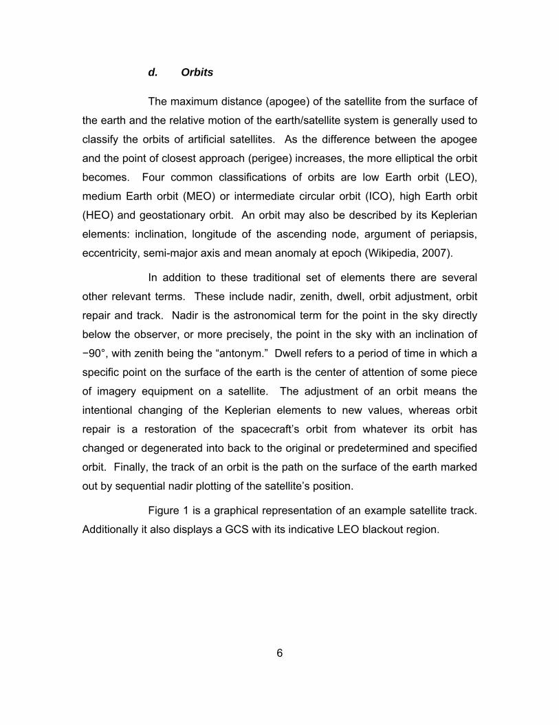
d. Orbits
The maximum distance (apogee) of the satellite from the surface of
the earth and the relative motion of the earth/satellite system is generally used to
classify the orbits of artificial satellites. As the difference between the apogee
and the point of closest approach (perigee) increases, the more elliptical the orbit
becomes. Four common classifications of orbits are low Earth orbit (LEO),
medium Earth orbit (MEO) or intermediate circular orbit (ICO), high Earth orbit
(HEO) and geostationary orbit. An orbit may also be described by its Keplerian
elements: inclination, longitude of the ascending node, argument of periapsis,
eccentricity, semi-major axis and mean anomaly at epoch (Wikipedia, 2007).
In addition to these traditional set of elements there are several
other relevant terms. These include nadir, zenith, dwell, orbit adjustment, orbit
repair and track. Nadir is the astronomical term for the point in the sky directly
below the observer, or more precisely, the point in the sky with an inclination of
−90°, with zenith being the “antonym.” Dwell refers to a period of time in which a
specific point on the surface of the earth is the center of attention of some piece
of imagery equipment on a satellite. The adjustment of an orbit means the
intentional changing of the Keplerian elements to new values, whereas orbit
repair is a restoration of the spacecraft’s orbit from whatever its orbit has
changed or degenerated into back to the original or predetermined and specified
orbit. Finally, the track of an orbit is the path on the surface of the earth marked
out by sequential nadir plotting of the satellite’s position.
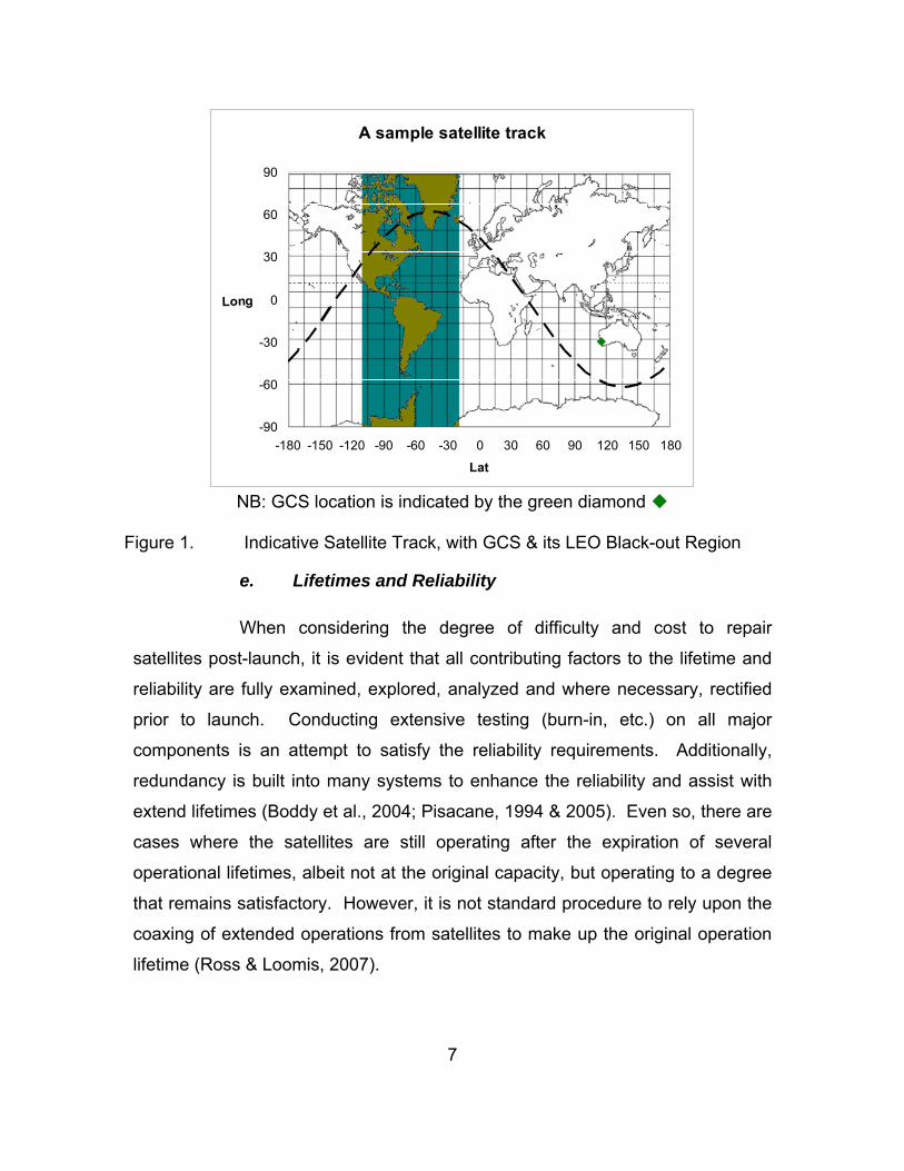
Figure 1 is a graphical representation of an example satellite track.
Additionally it also displays a GCS with its indicative LEO blackout region.
7
A sample satellite track
-90
-60
-30
0
30
60
90
-180 -150 -120 -90 -60 -30 0 30 60 90 120 150 180
Lat
Long
NB: GCS location is indicated by the green diamond
Figure 1. Indicative Satellite Track, with GCS & its LEO Black-out Region
e. Lifetimes and Reliability
When considering the degree of difficulty and cost to repair
satellites post-launch, it is evident that all contributing factors to the lifetime and
reliability are fully examined, explored, analyzed and where necessary, rectified
prior to launch. Conducting extensive testing (burn-in, etc.) on all major
components is an attempt to satisfy the reliability requirements. Additionally,
redundancy is built into many systems to enhance the reliability and assist with
extend lifetimes (Boddy et al., 2004; Pisacane, 1994 & 2005). Even so, there are
cases where the satellites are still operating after the expiration of several
operational lifetimes, albeit not at the original capacity, but operating to a degree
that remains satisfactory. However, it is not standard procedure to rely upon the
coaxing of extended operations from satellites to make up the original operation
lifetime (Ross & Loomis, 2007).
8
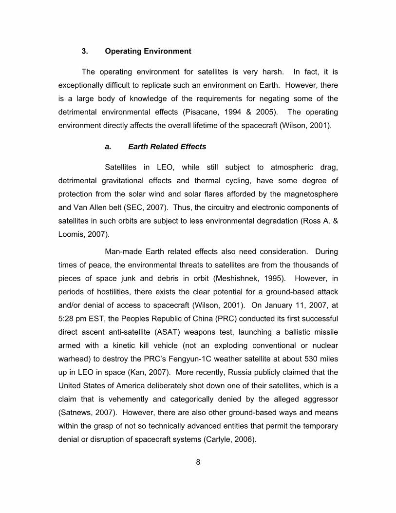
3. Operating Environment
The operating environment for satellites is very harsh. In fact, it is
exceptionally difficult to replicate such an environment on Earth. However, there
is a large body of knowledge of the requirements for negating some of the
detrimental environmental effects (Pisacane, 1994 & 2005). The operating
environment directly affects the overall lifetime of the spacecraft (Wilson, 2001).
a. Earth Related Effects
Satellites in LEO, while still subject to atmospheric drag,
detrimental gravitational effects and thermal cycling, have some degree of
protection from the solar wind and solar flares afforded by the magnetosphere
and Van Allen belt (SEC, 2007). Thus, the circuitry and electronic components of
satellites in such orbits are subject to less environmental degradation (Ross A. &
Loomis, 2007).
Man-made Earth related effects also need consideration. During
times of peace, the environmental threats to satellites are from the thousands of
pieces of space junk and debris in orbit (Meshishnek, 1995). However, in
periods of hostilities, there exists the clear potential for a ground-based attack
and/or denial of access to spacecraft (Wilson, 2001). On January 11, 2007, at
5:28 pm EST, the Peoples Republic of China (PRC) conducted its first successful
direct ascent anti-satellite (ASAT) weapons test, launching a ballistic missile
armed with a kinetic kill vehicle (not an exploding conventional or nuclear
warhead) to destroy the PRC’s Fengyun-1C weather satellite at about 530 miles
up in LEO in space (Kan, 2007). More recently, Russia publicly claimed that the
United States of America deliberately shot down one of their satellites, which is a
claim that is vehemently and categorically denied by the alleged aggressor
(Satnews, 2007). However, there are also other ground-based ways and means
within the grasp of not so technically advanced entities that permit the temporary
denial or disruption of spacecraft systems (Carlyle, 2006).
9
b. Helio Effects
In the case of higher orbits, the charge accumulation and
heightened radiation exposure from the Sun can lead to reduced lifetimes and
compromised reliability. Additionally, solar activity may be so intense that all
satellites are subject to some amount of degradation regardless of orbit
(Pisacane, 1994 & 2005; SEC, 2007).
4. Stochastic Markovian Analysis of Inoperability
Given comments above in regards to the threats to spacecraft operability
and despite the vast amount of resources invested in ensuring high standards of
reliability, there are various events that have the potential to cause spacecraft to
become inoperable, either temporarily or permanently. Using standard
procedures for the construction of Markov chains and some key assumptions
about the state transitions of the finite automata, a transition probability matrix, P,
may be developed (Ross S., 2003).
C. FINITE AUTOMATA (FA)
The finite automaton is a mathematical model of a system with discrete
inputs and outputs, often with discrete time intervals. The system can be in any
one of a finite number of internal configurations or “states.” The state of a
system summarizes the information concerning past inputs that is needed to
determine the behavior of the system on subsequent inputs (Hopcroft & Ullman,
1979).
1. Types of Finite Automata (FA)
The term finite automaton, finite automata (FA) in plural, includes a wide
range of related models including, but not limited to:
Deterministic finite automata (DFA),
Non-deterministic finite automata (NFA),
10
Two-way deterministic finite automata (2DFA),
Moore machines,
Mealy machines,
Deterministic pushdown automata (DPDA or PDA),
Non-deterministic pushdown automata (NPDA),
Turing machine (TM),
Non-deterministic Turing machine,
Multidimensional Turing machine,
Multi-head Turing machine, and
Off-line Turing machine, (Hennie, 1968; Hopcroft & Ullman, 1979).
The first of these is used in this thesis with some consideration given to
the second. Both non-deterministic finite automata (NFA) and pushdown
automata (PDA) models may provide some secondary utility. However, that is a
topic for further research.
2. Definition of FA
A FA, or in some instances a finite state automata (FSA) or finite state
machine (FSM), is a model of behavior composed of a finite number of states,
transitions between those states, and actions. By definition, the FA is in its start
state upon receipt of a procedure’s first input. Accept states are the subset of
final states, which represent the successful execution of the modeled procedure.
The transition function defines transitions between states that result from actions
as detailed or specified in the procedure, (Hopcroft & Ullman, 1979).
a. Transition Diagram
A graphical form of the transition function, namely the transition
diagram, is a directed graph that is associated with the FA and can be seen in
11
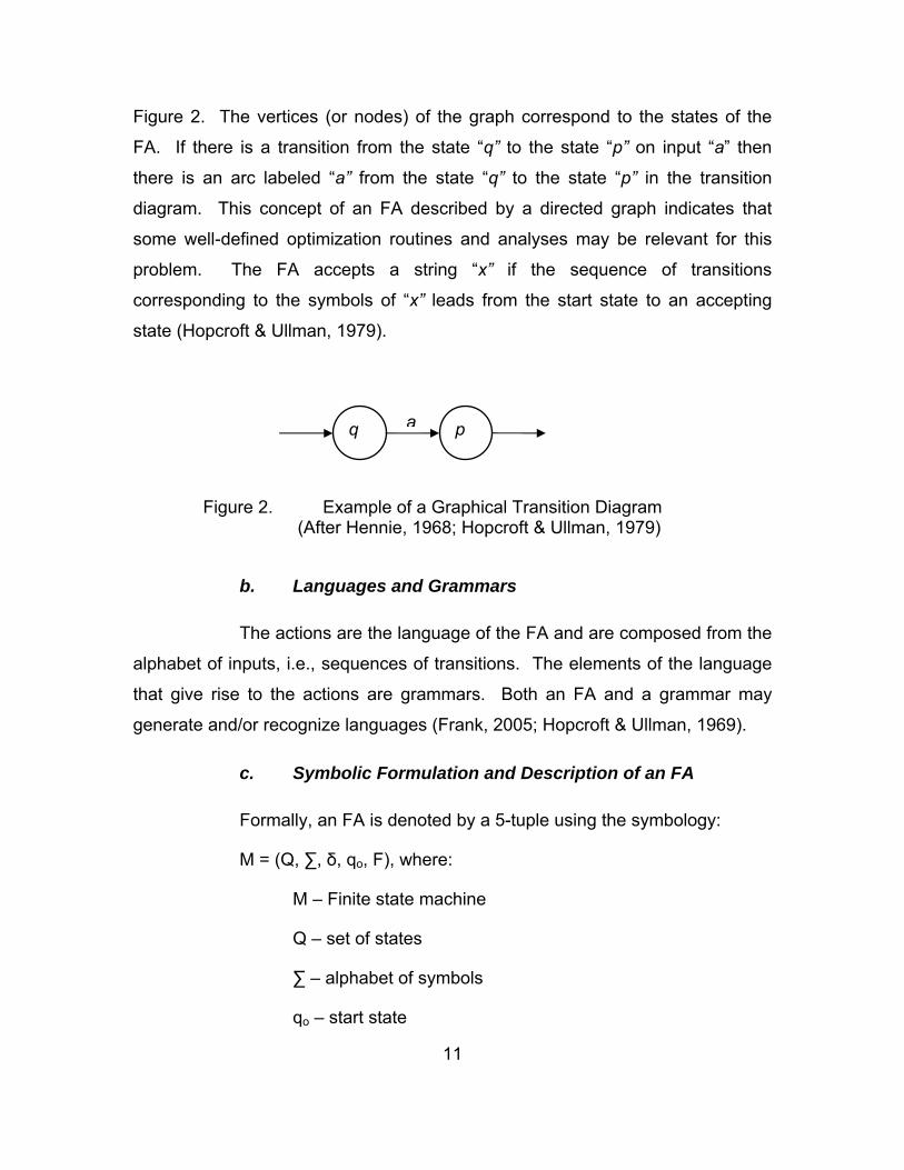
Figure 2. The vertices (or nodes) of the graph correspond to the states of the
FA. If there is a transition from the state “q” to the state “p” on input “a” then
there is an arc labeled “a” from the state “q” to the state “p” in the transition
diagram. This concept of an FA described by a directed graph indicates that
some well-defined optimization routines and analyses may be relevant for this
problem. The FA accepts a string “x” if the sequence of transitions
corresponding to the symbols of “x” leads from the start state to an accepting
state (Hopcroft & Ullman, 1979).
Figure 2. Example of a Graphical Transition Diagram
(After Hennie, 1968; Hopcroft & Ullman, 1979)
b. Languages and Grammars
The actions are the language of the FA and are composed from the
alphabet of inputs, i.e., sequences of transitions. The elements of the language
that give rise to the actions are grammars. Both an FA and a grammar may
generate and/or recognize languages (Frank, 2005; Hopcroft & Ullman, 1969).
c. Symbolic Formulation and Description of an FA
Formally, an FA is denoted by a 5-tuple using the symbology:
M = (Q, ∑, δ, qo, F), where:
M – Finite state machine
Q – set of states
∑ – alphabet of symbols
qo – start state
q p a
12
F – set of accept or final states
δ – transition function (Hopcroft & Ullman, 1979).
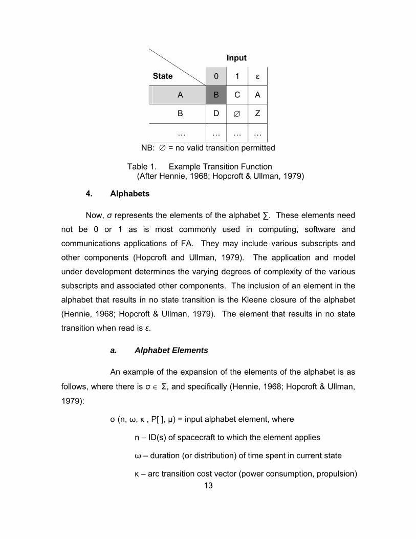
3. Transition Function
The concept of state transition for the FA can easily be visualized.
Consider a “tape” with a sequence of symbols “x” from the alphabet ∑ written on
it (Hopcroft & Ullman, 1979). A scanning head that reads the symbol as the tape
moves causes the machine to adopt the new state as determined by the state
prior to the reading of the symbol and the symbol itself. That is, if the FA is in
state “q” and the symbol “a” is scanned and there exists a path to “p” from “q”
given an input of “a,” then the resultant state is “p.” Symbolically this is:
δ(q, a) = p
A compact and functional method for displaying δ is to tabulate it (Hopcroft
& Ullman, 1979). The transition function is constructed from three components:
the list of states in the leftmost column, the list of inputs in the topmost row
excluding the first column and a table of states that reflect the valid transitions for
the input and state (read row and column) combinations. The transition function
is interpreted by selecting a “from” state in the left-hand column and selecting the
state from the intersection of that row and the column matching the next alphabet
element from “reading” the input stream. The selected state is the next “from”
state. For example, from the δ , as detailed in Table 1, starting in state A and
reading an input of 0 will cause the FA to go to state B.
13
Input
State 0 1 ε
A B C A
B D ∅ Z
… … … …
NB: ∅ = no valid transition permitted
Table 1. Example Transition Function (After Hennie, 1968; Hopcroft & Ullman, 1979)
4. Alphabets
Now, σ represents the elements of the alphabet ∑. These elements need
not be 0 or 1 as is most commonly used in computing, software and
communications applications of FA. They may include various subscripts and
other components (Hopcroft and Ullman, 1979). The application and model
under development determines the varying degrees of complexity of the various
subscripts and associated other components. The inclusion of an element in the
alphabet that results in no state transition is the Kleene closure of the alphabet
(Hennie, 1968; Hopcroft & Ullman, 1979). The element that results in no state
transition when read is ε.
a. Alphabet Elements
An example of the expansion of the elements of the alphabet is as
follows, where there is σ ∈ Σ, and specifically (Hennie, 1968; Hopcroft & Ullman,
1979):
σ (n, ω, κ , P[ ], µ) = input alphabet element, where
n – ID(s) of spacecraft to which the element applies
ω – duration (or distribution) of time spent in current state
κ – arc transition cost vector (power consumption, propulsion)
14
P[ ] – transition probability matrix for states of inoperability
µ – a vector of mean sojourn times for Inoperable states in P[ ]
This also includes the empty input element ε. Its symbology is:
ε (n, ω, κ, P[ ], µ).
b. Contribution to Network Formulations
Several notable features of this style of alphabet element design
and of the transition function assist in the optimization analysis. Firstly, in
considering the similarity of the FA to networks, arc costs could be considered as
duration of time, power consumption or mass of propulsion expended. Secondly,
the n is not limited to a single integer or integer pair but can be a forward star
array for complex, i.e., multiple, DSS. Lastly, the inclusion of stochastic terms ω.
P[ ], and µ permit a very expansive analysis and exploration of the solution
space. This is achieved via NFA where the model is repeatedly run until all the
desired state transitions have been enumerated, then transformed into a DFA for
analysis (Hennie, 1968; Volpano, 2007). This is beyond the scope of this thesis,
yet appears to be a promising field for further investigation.
5. Languages and Grammars
The natural extension is to include a set of symbols from the alphabet
rather than an individual symbol (Hopcroft & Ullman, 1979). These sets of
symbols or strings of elements from the alphabet are words. Additionally, these
words can also be joined together to form sentences or grammar for the FA –
thus defining a language. There a several types of languages used in
association with FA. These are regular languages (type 3), context-free
languages (CFL) (type 2), context-sensitive languages (type 1) and type 0. This
is the Chomsky Hierarchy of Languages (Frank, 2005). A formal grammar is a
quintuple, G = (∑, Φ, S, R), where:
15
∑ – alphabet of terminal symbols
Φ – alphabet of non-terminal symbols
S – start symbol
R – set of rules for sequences of symbols (Frank, 2005; Hopcroft &
Ullman, 1969).
Therefore, the language of a grammar L(G) or an FA L(M) is the set of
strings that can be derived from the start symbol, S, or start state, qo, according
to the description G = (∑, Φ, S, R) or M = (Q, ∑, δ, qo, F). In either case, the
protocols that define which transitions are permitted, i.e., the rule set or transition
function, factor directly into the language generated by the parent entity (Hennie,
1968). Hence for the case of an FA M, the formal symbolic description is:
L(M) = {ξ|δ(qo, ξ)∈F}, where:
qo – start state
δ – transition function
F – set of accept or final states
σ – the elements of the alphabet, ∑
ξ ⊂ {σ} – input strings composed from the elements of the alphabet.
These languages may be defined by regular expressions. As such, there
are a number of applicable operations. The set-theoretic operations include
union, intersection, difference and compliment. The language-theoretic
operations include concatenation, iteration and mirror Image. Regular languages
are those defined by the regular operators: union, concatenation and Kleene star.
These languages are closed under all above operations except mirror image
(Frank, 2005). The language L(M) accepted by the FA M, is a specific set, not
just any conglomeration of strings that transpire to be accepted by M (Hopcroft &
Ullman, 1979). The language L(M) is not an exhaustive path enumeration, but
moreover a prescribed collection of walks.
16
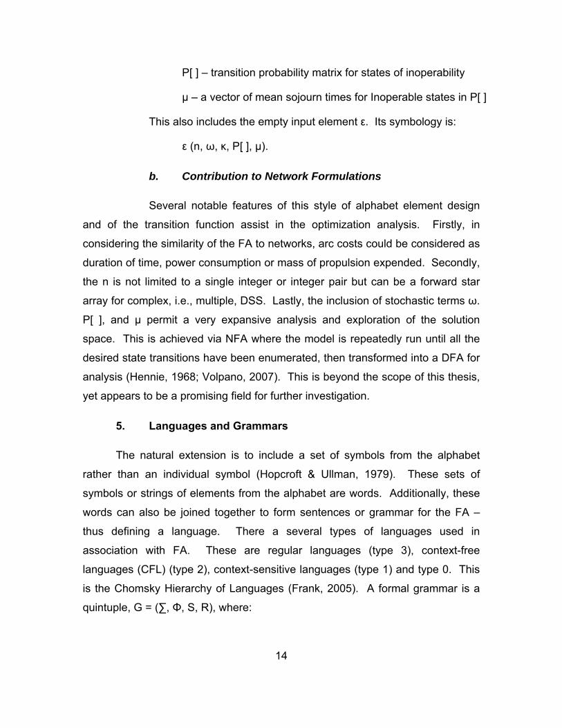
6. Language Similarities
It is interesting to note that there is an apparent relationship to and
between the normal, read ‘computer science’ or logical machine, constructs of
bits, bytes and words as well as the constructs of a language, L(M), generated by
the FA M. Table 2 unifies these ideas. In regards to the language, L(M),
developed for the DSS and an analysis of the quiddities of it and that used for
logical machine reveals the relationships described in the table below.
Additionally, the correspondence can be extended further to include some
elements of networks.
DSS FA component Logical Machine equivalent Network correspondence
Alphabet element Bit Arc cost or capacity
Task & meta-task Byte / word Shortest path
Table 2. Relationships between FA Components, Logical Machine & Network Concepts, (After Hopcroft & Ullman, 1979)
7. Non-deterministic Finite Automata (NFA)
Non-deterministic finite automata (NFA) are very similar to deterministic
finite automata (DFA) or (FA). A primary use is in the proving of theorems. The
one factor that separates NFA from FA is that for any same input there can be
more than one state transition from any one state—a node without degree
greater than one (Hopcroft & Ullman, 1979).
8. Amalgamation of FA
Conglomerations of NFA and/or FA are used to determine if an NFA will
accept a given input string (Hopcroft & Ullman, 1979). The NFA may be
sequenced consecutively or in parallel with a minimal offset (Hopcroft & Ullman,
1979). The use of NFA could prove very worthwhile for further research into this
problem.
17
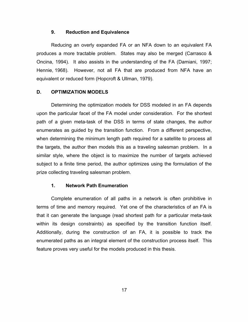
9. Reduction and Equivalence
Reducing an overly expanded FA or an NFA down to an equivalent FA
produces a more tractable problem. States may also be merged (Carrasco &
Oncina, 1994). It also assists in the understanding of the FA (Damiani, 1997;
Hennie, 1968). However, not all FA that are produced from NFA have an
equivalent or reduced form (Hopcroft & Ullman, 1979).
D. OPTIMIZATION MODELS
Determining the optimization models for DSS modeled in an FA depends
upon the particular facet of the FA model under consideration. For the shortest
path of a given meta-task of the DSS in terms of state changes, the author
enumerates as guided by the transition function. From a different perspective,
when determining the minimum length path required for a satellite to process all
the targets, the author then models this as a traveling salesman problem. In a
similar style, where the object is to maximize the number of targets achieved
subject to a finite time period, the author optimizes using the formulation of the
prize collecting traveling salesman problem.
1. Network Path Enumeration
Complete enumeration of all paths in a network is often prohibitive in
terms of time and memory required. Yet one of the characteristics of an FA is
that it can generate the language (read shortest path for a particular meta-task
within its design constraints) as specified by the transition function itself.
Additionally, during the construction of an FA, it is possible to track the
enumerated paths as an integral element of the construction process itself. This
feature proves very useful for the models produced in this thesis.
18
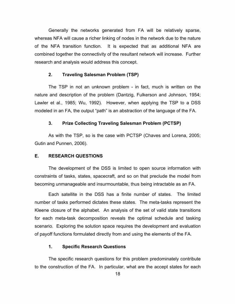
Generally the networks generated from FA will be relatively sparse,
whereas NFA will cause a richer linking of nodes in the network due to the nature
of the NFA transition function. It is expected that as additional NFA are
combined together the connectivity of the resultant network will increase. Further
research and analysis would address this concept.
2. Traveling Salesman Problem (TSP)
The TSP in not an unknown problem - in fact, much is written on the
nature and description of the problem (Dantzig, Fulkerson and Johnson, 1954;
Lawler et al., 1985; Wu, 1992). However, when applying the TSP to a DSS
modeled in an FA, the output “path” is an abstraction of the language of the FA.
3. Prize Collecting Traveling Salesman Problem (PCTSP)
As with the TSP, so is the case with PCTSP (Chaves and Lorena, 2005;
Gutin and Punnen, 2006).
E. RESEARCH QUESTIONS
The development of the DSS is limited to open source information with
constraints of tasks, states, spacecraft, and so on that preclude the model from
becoming unmanageable and insurmountable, thus being intractable as an FA.
Each satellite in the DSS has a finite number of states. The limited
number of tasks performed dictates these states. The meta-tasks represent the
Kleene closure of the alphabet. An analysis of the set of valid state transitions
for each meta-task decomposition reveals the optimal schedule and tasking
scenario. Exploring the solution space requires the development and evaluation
of payoff functions formulated directly from and using the elements of the FA.
1. Specific Research Questions
The specific research questions for this problem predominately contribute
to the construction of the FA. In particular, what are the accept states for each
19
agent in the multi-agent system, what are the meta-tasks and what is the
alphabet? Then, constructing a transition function permits the design and
explanation of a representational FSA for this problem. Finally, given an
indicative sample target set, what is the minimum time for a single spacecraft to
process all targets and what is the maximum number of targets that a single
spacecraft can process in a time-constrained mission?
2. Potential Research Extensions
Given that this interdisciplinary thesis is largely an explorative venture the
pursuit of the research is predominately focused in developing initial concepts.
However, discrete event simulations (DES), arising from discrete event graphs,
can be mapped to mathematical programming problems (Chan, 2005; Chan &
Schruben, 2003, 2005 & 2006), yet there is an apparent dearth of knowledge for
such procedures for FSA (Tung & Kleinrock, 1996; Yang et al., 1994). This
problem warrants further research in this field. Exploiting the FA/DES duality
relationship (Sanchez, 2006) and then applying the extant of modified DES
mapping procedures may provide an indirect or heuristic method for the FA
formulations. This level of investigation is beyond the scope of this thesis.

20
THIS PAGE INTENTIONALLY LEFT BLANK
21
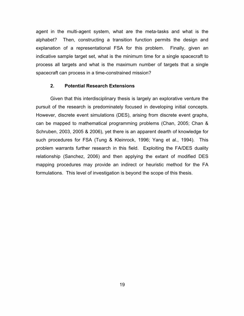
III. THE MODELS
A. MODEL DISCUSSION
The FA models developed in this thesis capture the essential elements
and relationships of DSS (Horning, 2006; Ross I.M., 2007). Where actual data is
not available, the author approximates values for real world parameters
(Ross I.M., 2007).
B. DSS CHARACTERISTICS
In order to develop a preliminary model, a number of assumptions about
DSS are required and are discussed below.
1. Orbit Assumptions
The management of orbits is a non-trivial pursuit (Avanzini et al., 2004).
Although quaternion-based mathematics is often used (Joly, 1905; Kuipers,
1999), the author adopted a simpler approach. The orbit assumptions include
the direction of orbit, orbit deconfliction and other orbit parameters. The direction
of orbit is assumed to be anti-clockwise, i.e., the satellite transmits from west to
east across the face of the globe. The orbits of multiple satellites are sufficiently
out of phase that deconfliction is automatic. In regards to the orbit parameters,
not all of the Keplerian elements are used in this simplified model. The orbit
parameters for the single spacecraft model are detailed in Table 3.
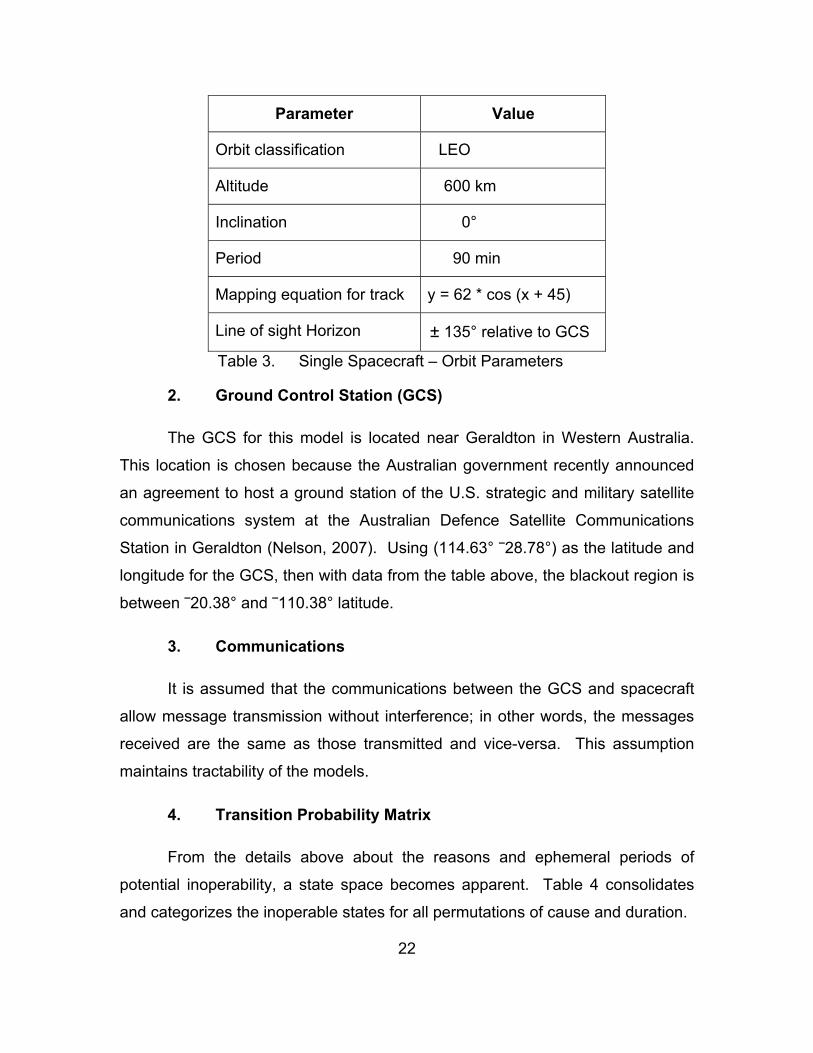
22
Parameter Value
Orbit classification LEO
Altitude 600 km
Inclination 0°
Period 90 min
Mapping equation for track y = 62 * cos (x + 45)
Line of sight Horizon ± 135° relative to GCS
Table 3. Single Spacecraft – Orbit Parameters
2. Ground Control Station (GCS)
The GCS for this model is located near Geraldton in Western Australia.
This location is chosen because the Australian government recently announced
an agreement to host a ground station of the U.S. strategic and military satellite
communications system at the Australian Defence Satellite Communications
Station in Geraldton (Nelson, 2007). Using (114.63° –28.78°) as the latitude and
longitude for the GCS, then with data from the table above, the blackout region is
between –20.38° and –110.38° latitude.
3. Communications
It is assumed that the communications between the GCS and spacecraft
allow message transmission without interference; in other words, the messages
received are the same as those transmitted and vice-versa. This assumption
maintains tractability of the models.
4. Transition Probability Matrix
From the details above about the reasons and ephemeral periods of
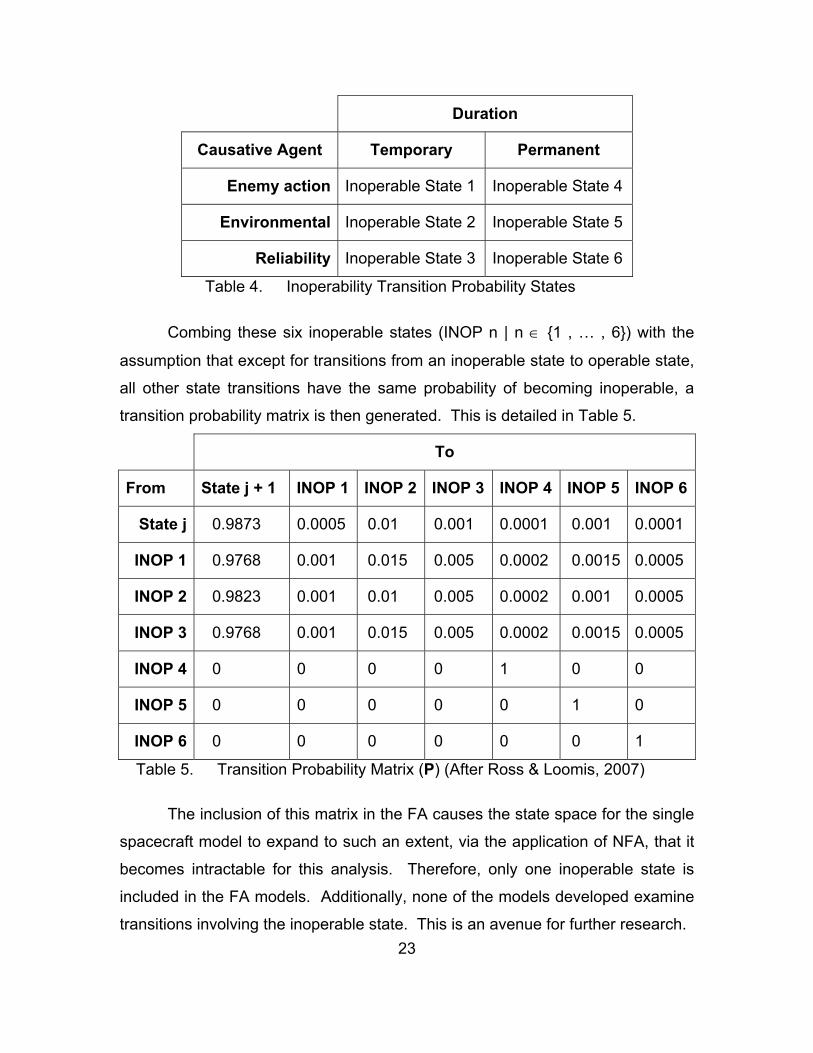
potential inoperability, a state space becomes apparent. Table 4 consolidates
and categorizes the inoperable states for all permutations of cause and duration.
23
Duration
Causative Agent Temporary Permanent
Enemy action Inoperable State 1 Inoperable State 4
Environmental Inoperable State 2 Inoperable State 5
Reliability Inoperable State 3 Inoperable State 6
Table 4. Inoperability Transition Probability States
Combing these six inoperable states (INOP n | n ∈ {1 , … , 6}) with the
assumption that except for transitions from an inoperable state to operable state,
all other state transitions have the same probability of becoming inoperable, a
transition probability matrix is then generated. This is detailed in Table 5.
To
From State j + 1 INOP 1 INOP 2 INOP 3 INOP 4 INOP 5 INOP 6
State j 0.9873 0.0005 0.01 0.001 0.0001 0.001 0.0001
INOP 1 0.9768 0.001 0.015 0.005 0.0002 0.0015 0.0005
INOP 2 0.9823 0.001 0.01 0.005 0.0002 0.001 0.0005
INOP 3 0.9768 0.001 0.015 0.005 0.0002 0.0015 0.0005
INOP 4 0 0 0 0 1 0 0
INOP 5 0 0 0 0 0 1 0
INOP 6 0 0 0 0 0 0 1
Table 5. Transition Probability Matrix (P) (After Ross & Loomis, 2007)
The inclusion of this matrix in the FA causes the state space for the single
spacecraft model to expand to such an extent, via the application of NFA, that it
becomes intractable for this analysis. Therefore, only one inoperable state is
included in the FA models. Additionally, none of the models developed examine
transitions involving the inoperable state. This is an avenue for further research.
24
C. SINGLE SPACECRAFT FA
Recalling that the symbolic description of an FA is:
M = (Q, ∑, δ, qo, F), where:
M – Finite state machine
Q – set of states
∑ – alphabet of symbols
qo – start state
F – set of accept or final states
δ – transition function, (Hopcroft & Ullman, 1979).
and given that elements of the alphabet may be subscripted or otherwise
annotated (Hopcroft & Ullman, 1979), the author defines them as:
σ (n, ω, κ , P[ ], µ) = input alphabet element, where
n – ID of spacecraft to which the element applies
ω – duration (or distribution) of time spent in current state
κ – arc transition cost vector (power consumption, propulsion)
P[ ] – transition probability matrix for states of inoperability
µ – a vector of mean sojourn times for Inoperable states in P[ ]
The author presents the single spacecraft model in Tables 6 to 8 with
some interspersed amplifying comments.
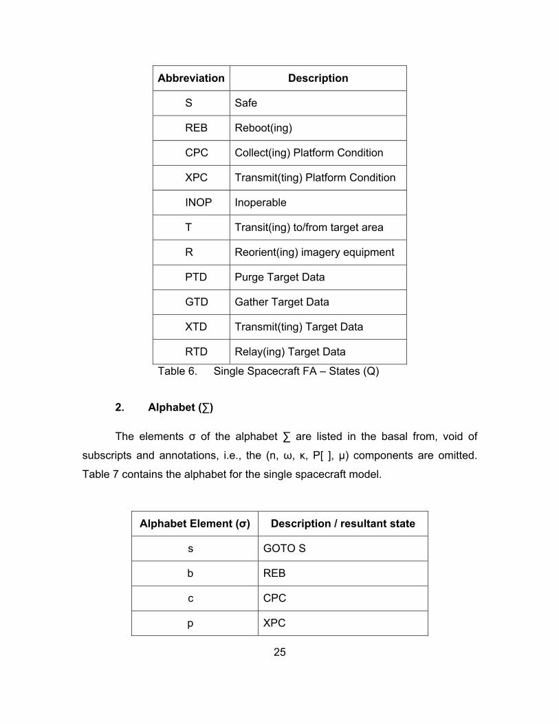
1. States (Q)
Table 6 details the states of the single spacecraft model.
25
Abbreviation Description
S Safe
REB Reboot(ing)
CPC Collect(ing) Platform Condition
XPC Transmit(ting) Platform Condition
INOP Inoperable
T Transit(ing) to/from target area
R Reorient(ing) imagery equipment
PTD Purge Target Data
GTD Gather Target Data
XTD Transmit(ting) Target Data
RTD Relay(ing) Target Data
Table 6. Single Spacecraft FA – States (Q)
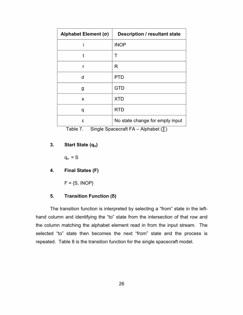
2. Alphabet (∑)
The elements σ of the alphabet ∑ are listed in the basal from, void of
subscripts and annotations, i.e., the (n, ω, κ, P[ ], µ) components are omitted.
Table 7 contains the alphabet for the single spacecraft model.
Alphabet Element (σ) Description / resultant state
s GOTO S
b REB
c CPC
p XPC
26
Alphabet Element (σ) Description / resultant state
i INOP
t T
r R
d PTD
g GTD
x XTD
q RTD
ε No state change for empty input
Table 7. Single Spacecraft FA – Alphabet (∑)
3. Start State (qo)
qo = S
4. Final States (F)
F = {S, INOP}
5. Transition Function (δ)
The transition function is interpreted by selecting a “from” state in the left-
hand column and identifying the “to” state from the intersection of that row and
the column matching the alphabet element read in from the input stream. The
selected “to” state then becomes the next “from” state and the process is
repeated. Table 8 is the transition function for the single spacecraft model.
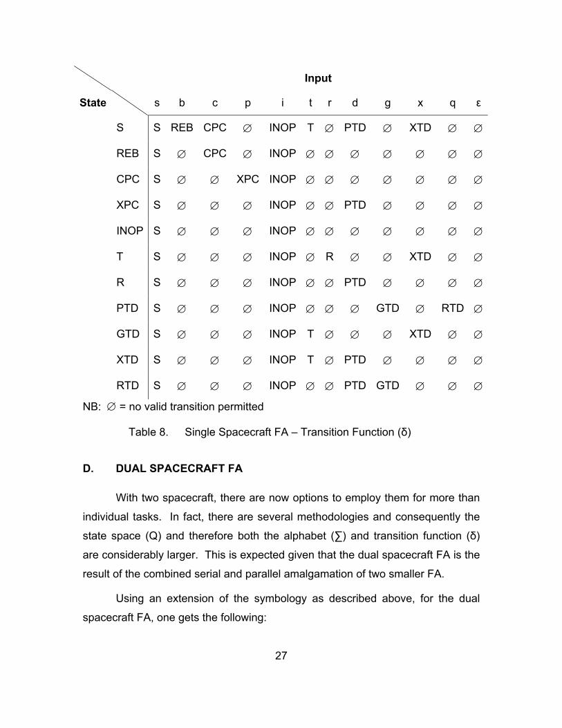
27
Input
State s b c p i t r d g x q ε
S S REB CPC ∅ INOP T ∅ PTD ∅ XTD ∅ ∅
REB S ∅ CPC ∅ INOP ∅ ∅ ∅ ∅ ∅ ∅ ∅
CPC S ∅ ∅ XPC INOP ∅ ∅ ∅ ∅ ∅ ∅ ∅
XPC S ∅ ∅ ∅ INOP ∅ ∅ PTD ∅ ∅ ∅ ∅
INOP S ∅ ∅ ∅ INOP ∅ ∅ ∅ ∅ ∅ ∅ ∅
T S ∅ ∅ ∅ INOP ∅ R ∅ ∅ XTD ∅ ∅
R S ∅ ∅ ∅ INOP ∅ ∅ PTD ∅ ∅ ∅ ∅
PTD S ∅ ∅ ∅ INOP ∅ ∅ ∅ GTD ∅ RTD ∅
GTD S ∅ ∅ ∅ INOP T ∅ ∅ ∅ XTD ∅ ∅
XTD S ∅ ∅ ∅ INOP T ∅ PTD ∅ ∅ ∅ ∅
RTD S ∅ ∅ ∅ INOP ∅ ∅ PTD GTD ∅ ∅ ∅
NB: ∅ = no valid transition permitted
Table 8. Single Spacecraft FA – Transition Function (δ)
D. DUAL SPACECRAFT FA
With two spacecraft, there are now options to employ them for more than
individual tasks. In fact, there are several methodologies and consequently the
state space (Q) and therefore both the alphabet (∑) and transition function (δ)
are considerably larger. This is expected given that the dual spacecraft FA is the
result of the combined serial and parallel amalgamation of two smaller FA.
Using an extension of the symbology as described above, for the dual
spacecraft FA, one gets the following:
28
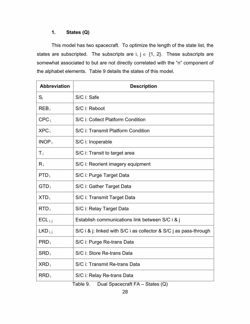
1. States (Q)
This model has two spacecraft. To optimize the length of the state list, the
states are subscripted. The subscripts are i, j ∈ {1, 2}. These subscripts are
somewhat associated to but are not directly correlated with the “n” component of
the alphabet elements. Table 9 details the states of this model.
Abbreviation Description
Si S/C i: Safe
REB i S/C i: Reboot
CPC i S/C i: Collect Platform Condition
XPC i S/C i: Transmit Platform Condition
INOP i S/C i: Inoperable
T i S/C i: Transit to target area
R i S/C i: Reorient imagery equipment
PTD i S/C i: Purge Target Data
GTD i S/C i: Gather Target Data
XTD i S/C i: Transmit Target Data
RTD i S/C i: Relay Target Data
ECL i, j Establish communications link between S/C i & j
LKD i, j S/C i & j: linked with S/C i as collector & S/C j as pass-through
PRD i S/C i: Purge Re-trans Data
SRD i S/C i: Store Re-trans Data
XRD i S/C i: Transmit Re-trans Data
RRD i S/C i: Relay Re-trans Data
Table 9. Dual Spacecraft FA – States (Q)
29
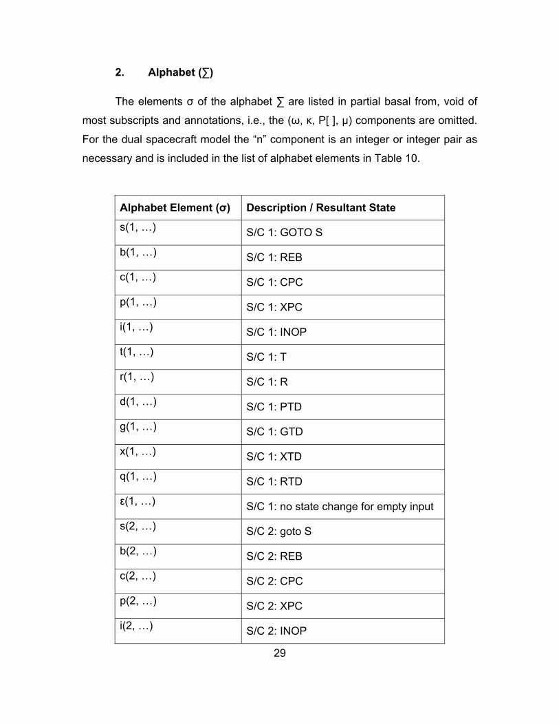
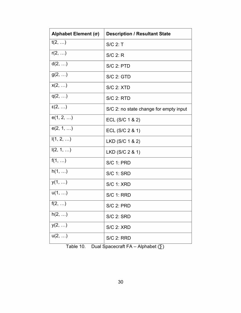
2. Alphabet (∑)
The elements σ of the alphabet ∑ are listed in partial basal from, void of
most subscripts and annotations, i.e., the (ω, κ, P[ ], µ) components are omitted.
For the dual spacecraft model the “n” component is an integer or integer pair as
necessary and is included in the list of alphabet elements in Table 10.
Alphabet Element (σ) Description / Resultant State
s(1, …) S/C 1: GOTO S
b(1, …) S/C 1: REB
c(1, …) S/C 1: CPC
p(1, …) S/C 1: XPC
i(1, …) S/C 1: INOP
t(1, …) S/C 1: T
r(1, …) S/C 1: R
d(1, …) S/C 1: PTD
g(1, …) S/C 1: GTD
x(1, …) S/C 1: XTD
q(1, …) S/C 1: RTD
ε(1, …) S/C 1: no state change for empty input
s(2, …) S/C 2: goto S
b(2, …) S/C 2: REB
c(2, …) S/C 2: CPC
p(2, …) S/C 2: XPC
i(2, …) S/C 2: INOP
30
Alphabet Element (σ) Description / Resultant State
t(2, …) S/C 2: T
r(2, …) S/C 2: R
d(2, …) S/C 2: PTD
g(2, …) S/C 2: GTD
x(2, …) S/C 2: XTD
q(2, …) S/C 2: RTD
ε(2, …) S/C 2: no state change for empty input
e(1, 2, …) ECL (S/C 1 & 2)
e(2, 1, …) ECL (S/C 2 & 1)
l(1, 2, …) LKD (S/C 1 & 2)
l(2, 1, …) LKD (S/C 2 & 1)
f(1, …) S/C 1: PRD
h(1, …) S/C 1: SRD
y(1, …) S/C 1: XRD
u(1, …) S/C 1: RRD
f(2, …) S/C 2: PRD
h(2, …) S/C 2: SRD
y(2, …) S/C 2: XRD
u(2, …) S/C 2: RRD
Table 10. Dual Spacecraft FA – Alphabet (∑)
31
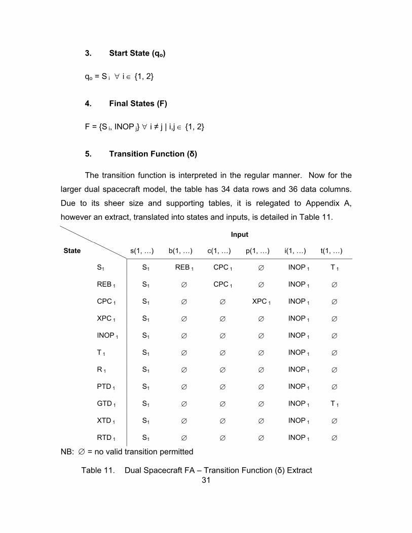
3. Start State (qo)
qo = S i ∀ i ∈ {1, 2}
4. Final States (F)
F = {S i, INOP j} ∀ i ≠ j | i,j ∈ {1, 2}
5. Transition Function (δ)
The transition function is interpreted in the regular manner. Now for the
larger dual spacecraft model, the table has 34 data rows and 36 data columns.
Due to its sheer size and supporting tables, it is relegated to Appendix A,
however an extract, translated into states and inputs, is detailed in Table 11.
Input
State s(1, …) b(1, …) c(1, …) p(1, …) i(1, …) t(1, …)
S1 S1 REB 1 CPC 1 ∅ INOP 1 T 1
REB 1 S1 ∅ CPC 1 ∅ INOP 1 ∅
CPC 1 S1 ∅ ∅ XPC 1 INOP 1 ∅
XPC 1 S1 ∅ ∅ ∅ INOP 1 ∅
INOP 1 S1 ∅ ∅ ∅ INOP 1 ∅
T 1 S1 ∅ ∅ ∅ INOP 1 ∅
R 1 S1 ∅ ∅ ∅ INOP 1 ∅
PTD 1 S1 ∅ ∅ ∅ INOP 1 ∅
GTD 1 S1 ∅ ∅ ∅ INOP 1 T 1
XTD 1 S1 ∅ ∅ ∅ INOP 1 ∅
RTD 1 S1 ∅ ∅ ∅ INOP 1 ∅
NB: ∅ = no valid transition permitted
Table 11. Dual Spacecraft FA – Transition Function (δ) Extract
32
E. LANGUAGE OF THE MODELS – L(M)
The languages that each of the FA generate are similar. In order to
construct the languages L(M), “sentences” are required. These “sentences” are
themselves constructed of “words” ξ. Moreover, the “words” are constructed
from the elements σ of the alphabets ∑ of each of the models as detailed above.
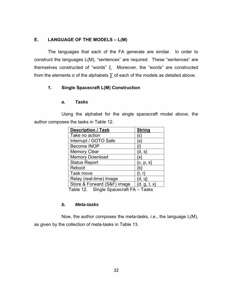
1. Single Spacecraft L(M) Construction
a. Tasks
Using the alphabet for the single spacecraft model above, the
author composes the tasks in Table 12.
Description / Task String Take no action {ε} Interrupt / GOTO Safe {s} Become INOP {i} Memory Clear {d, s} Memory Download {x} Status Report {c, p, s} Reboot {b} Task move {t, r} Relay (real-time) Image {d, q} Store & Forward (S&F) image {d, g, t, x}
Table 12. Single Spacecraft FA – Tasks
b. Meta-tasks
Now, the author composes the meta-tasks, i.e., the language L(M),
as given by the collection of meta-tasks in Table 13.
33
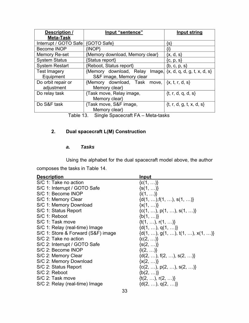
Description / Meta-Task
Input “sentence” Input string
Interrupt / GOTO Safe {GOTO Safe} {s} Become INOP {INOP} {i} Memory Re-set {Memory download, Memory clear} {x, d, s} System Status {Status report} {c, p, s} System Restart {Reboot, Status report} {b, c, p, s} Test Imagery Equipment
{Memory download, Relay Image,S&F image, Memory clear
{x, d, q, d, g, t, x, d, s}
Do orbit repair or adjustment
{Memory download, Task move, Memory clear}
{x, t, r, d, s}
Do relay task {Task move, Relay image, Memory clear}
{t, r, d, q, d, s}
Do S&F task {Task move, S&F image, Memory clear}
{t, r, d, g, t, x, d, s}
Table 13. Single Spacecraft FA – Meta-tasks
2. Dual spacecraft L(M) Construction
a. Tasks
Using the alphabet for the dual spacecraft model above, the author
composes the tasks in Table 14.
Description Input S/C 1: Take no action {ε(1, …)} S/C 1: Interrupt / GOTO Safe {s(1, …)} S/C 1: Become INOP {i(1, …)} S/C 1: Memory Clear {d(1, …),f(1, …), s(1, …)} S/C 1: Memory Download {x(1, …)} S/C 1: Status Report {c(1, …), p(1, …), s(1, …)} S/C 1: Reboot {b(1, …)} S/C 1: Task move {t(1, …), r(1, …)} S/C 1: Relay (real-time) Image {d(1, …), q(1, …)} S/C 1: Store & Forward (S&F) image {d(1, …), g(1, …), t(1, …), x(1, …)} S/C 2: Take no action {ε(2, …)} S/C 2: Interrupt / GOTO Safe {s(2, …)} S/C 2: Become INOP {i(2, …)} S/C 2: Memory Clear {d(2, …), f(2, …), s(2, …)} S/C 2: Memory Download {x(2, …)} S/C 2: Status Report {c(2, …), p(2, …), s(2, …)} S/C 2: Reboot {b(2, …)} S/C 2: Task move {t(2, …), r(2, …)} S/C 2: Relay (real-time) Image {d(2, …), q(2, …)}
34
S/C 2: S&F image {d(2, …), g(2, …), t(2, …), x(2, …)} S/C 1 & 2: Prep for joint task {e(1,2, …), l(1,2…)} S/C 2: Relay (real-time) re-trans data {f(2, …), u(2…)} S/C 2: Store re-trans data {f(2…), h(2…)} S/C 2: Forward re-trans data {t(2, …), y(2…)} S/C 2 & 1: Prep for joint task {e(2,1, …), l(2,1…)} S/C 1: Relay (real-time) re-trans data {f(1, …), u(1…)} S/C 1: Store re-trans data {f(1…), h(1…)} S/C 1: Forward re-trans data {t(1, …), y(1…)}
Table 14. Dual Spacecraft FA – Tasks
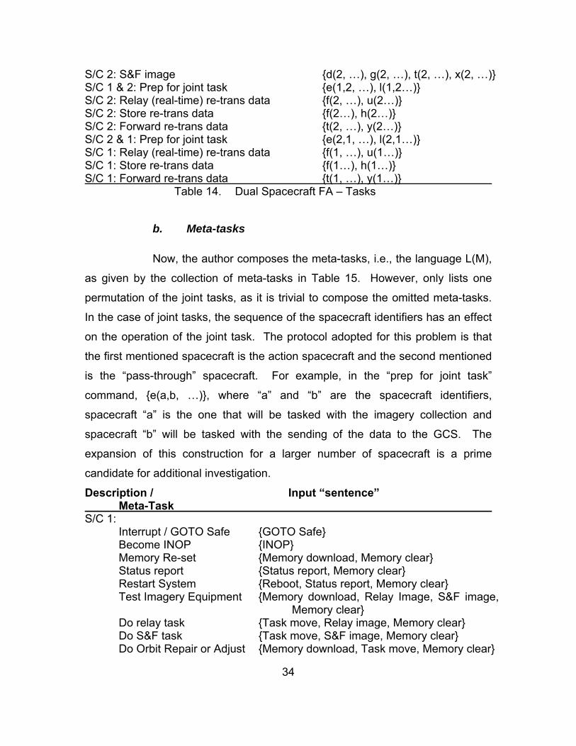
b. Meta-tasks
Now, the author composes the meta-tasks, i.e., the language L(M),
as given by the collection of meta-tasks in Table 15. However, only lists one
permutation of the joint tasks, as it is trivial to compose the omitted meta-tasks.
In the case of joint tasks, the sequence of the spacecraft identifiers has an effect
on the operation of the joint task. The protocol adopted for this problem is that
the first mentioned spacecraft is the action spacecraft and the second mentioned
is the “pass-through” spacecraft. For example, in the “prep for joint task”
command, {e(a,b, …)}, where “a” and “b” are the spacecraft identifiers,
spacecraft “a” is the one that will be tasked with the imagery collection and
spacecraft “b” will be tasked with the sending of the data to the GCS. The
expansion of this construction for a larger number of spacecraft is a prime
candidate for additional investigation.
Description / Input “sentence” Meta-Task S/C 1:
Interrupt / GOTO Safe {GOTO Safe} Become INOP {INOP} Memory Re-set {Memory download, Memory clear} Status report {Status report, Memory clear} Restart System {Reboot, Status report, Memory clear} Test Imagery Equipment {Memory download, Relay Image, S&F image,
Memory clear} Do relay task {Task move, Relay image, Memory clear} Do S&F task {Task move, S&F image, Memory clear} Do Orbit Repair or Adjust {Memory download, Task move, Memory clear}
35
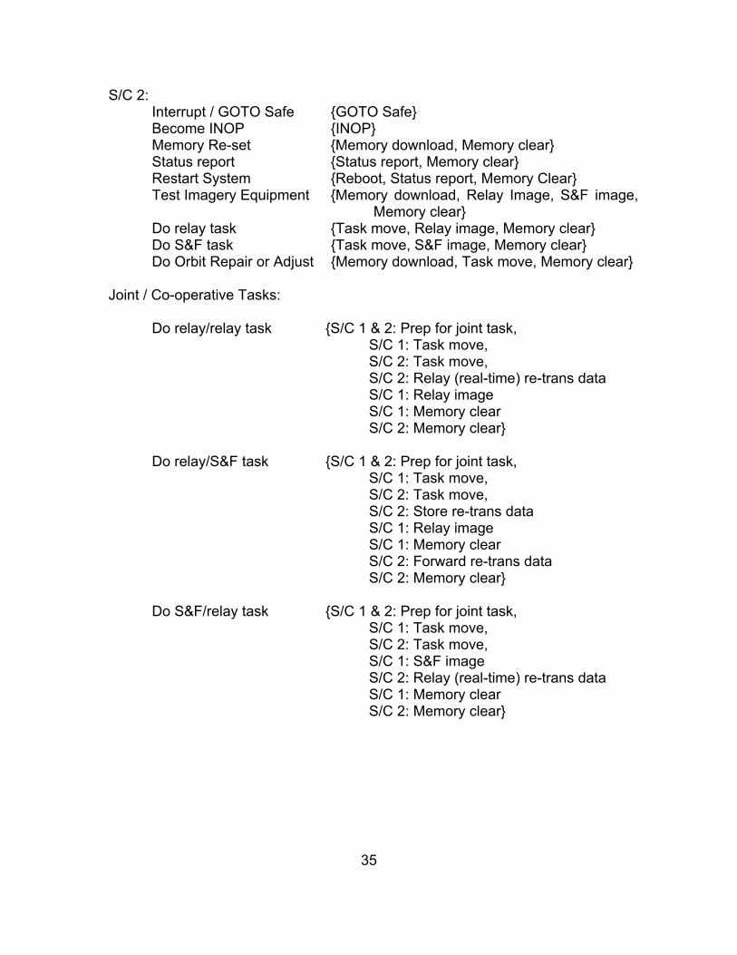
S/C 2: Interrupt / GOTO Safe {GOTO Safe} Become INOP {INOP} Memory Re-set {Memory download, Memory clear} Status report {Status report, Memory clear} Restart System {Reboot, Status report, Memory Clear} Test Imagery Equipment {Memory download, Relay Image, S&F image,
Memory clear} Do relay task {Task move, Relay image, Memory clear} Do S&F task {Task move, S&F image, Memory clear} Do Orbit Repair or Adjust {Memory download, Task move, Memory clear}
Joint / Co-operative Tasks:
Do relay/relay task {S/C 1 & 2: Prep for joint task, S/C 1: Task move, S/C 2: Task move, S/C 2: Relay (real-time) re-trans data S/C 1: Relay image S/C 1: Memory clear S/C 2: Memory clear} Do relay/S&F task {S/C 1 & 2: Prep for joint task, S/C 1: Task move, S/C 2: Task move, S/C 2: Store re-trans data S/C 1: Relay image S/C 1: Memory clear S/C 2: Forward re-trans data S/C 2: Memory clear} Do S&F/relay task {S/C 1 & 2: Prep for joint task, S/C 1: Task move, S/C 2: Task move, S/C 1: S&F image S/C 2: Relay (real-time) re-trans data S/C 1: Memory clear S/C 2: Memory clear}
36
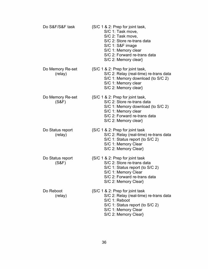
Do S&F/S&F task {S/C 1 & 2: Prep for joint task, S/C 1: Task move, S/C 2: Task move, S/C 2: Store re-trans data S/C 1: S&F image S/C 1: Memory clear S/C 2: Forward re-trans data S/C 2: Memory clear} Do Memory Re-set {S/C 1 & 2: Prep for joint task, (relay) S/C 2: Relay (real-time) re-trans data S/C 1: Memory download (to S/C 2) S/C 1: Memory clear S/C 2: Memory clear} Do Memory Re-set {S/C 1 & 2: Prep for joint task, (S&F) S/C 2: Store re-trans data S/C 1: Memory download (to S/C 2) S/C 1: Memory clear S/C 2: Forward re-trans data S/C 2: Memory clear} Do Status report {S/C 1 & 2: Prep for joint task (relay) S/C 2: Relay (real-time) re-trans data S/C 1: Status report (to S/C 2) S/C 1: Memory Clear S/C 2: Memory Clear} Do Status report {S/C 1 & 2: Prep for joint task (S&F) S/C 2: Store re-trans data S/C 1: Status report (to S/C 2) S/C 1: Memory Clear S/C 2: Forward re-trans data S/C 2: Memory Clear} Do Reboot {S/C 1 & 2: Prep for joint task (relay) S/C 2: Relay (real-time) re-trans data S/C 1: Reboot S/C 1: Status report (to S/C 2) S/C 1: Memory Clear S/C 2: Memory Clear}
37
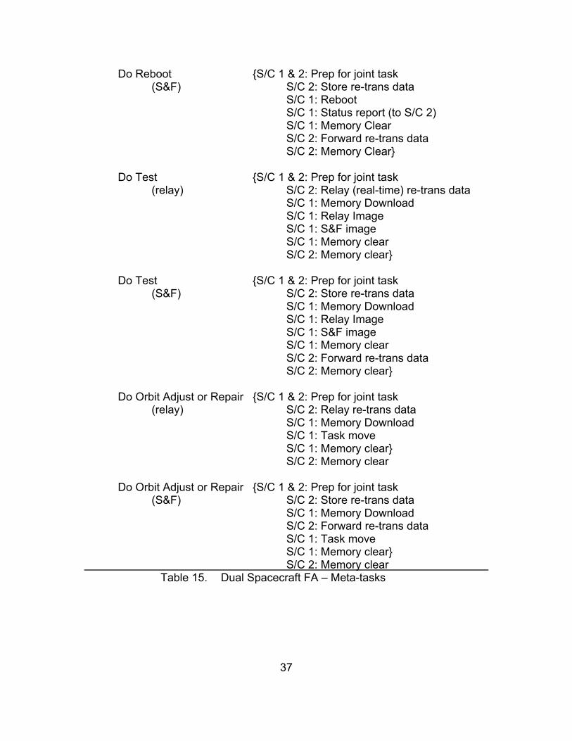
Do Reboot {S/C 1 & 2: Prep for joint task (S&F) S/C 2: Store re-trans data S/C 1: Reboot S/C 1: Status report (to S/C 2) S/C 1: Memory Clear S/C 2: Forward re-trans data S/C 2: Memory Clear} Do Test {S/C 1 & 2: Prep for joint task (relay) S/C 2: Relay (real-time) re-trans data S/C 1: Memory Download S/C 1: Relay Image S/C 1: S&F image S/C 1: Memory clear S/C 2: Memory clear} Do Test {S/C 1 & 2: Prep for joint task (S&F) S/C 2: Store re-trans data S/C 1: Memory Download S/C 1: Relay Image S/C 1: S&F image S/C 1: Memory clear S/C 2: Forward re-trans data S/C 2: Memory clear} Do Orbit Adjust or Repair {S/C 1 & 2: Prep for joint task (relay) S/C 2: Relay re-trans data S/C 1: Memory Download S/C 1: Task move S/C 1: Memory clear} S/C 2: Memory clear
Do Orbit Adjust or Repair {S/C 1 & 2: Prep for joint task (S&F) S/C 2: Store re-trans data S/C 1: Memory Download S/C 2: Forward re-trans data S/C 1: Task move S/C 1: Memory clear}
S/C 2: Memory clear Table 15. Dual Spacecraft FA – Meta-tasks
38
F. GRAPHICAL REPRESENTATIONS
Both of the FA developed for this problem may be put into a graphical
format. This format permits a simple pictorial representation of the FA in which
its human readability and comprehension are significantly enhanced. Various
other methods exist. These include the MATLAB STATEFLOW and SIMULINK
libraries (MATLAB, 2007; Moscinski & Ogonowski, 1995), a statechart
representation (Harel, 1987), a graph theory version (Hunt, 2002) and others
(Frasconi et al., 1996; Radivojevic & Brewer, 1994). It is recommended that
further research into this problem commence with the development of a graphical
representation of the FA developed herein.
G. MATLAB
The implementation of the single spacecraft model in MATLAB is a
provisional proof of concept. It provides the rudimentary elements of the FA and
a clear initiation point for further development (Broadston, 2007). Appendix B
details the code for the MATLAB implementation of the single spacecraft model.
39
IV. TARGETRY OPTIMIZATION
A. TARGETRY MODEL
The model for the targetry consists of eight targets uniformly distributed
across the face of the globe. Although the number of targets is only an indicative
figure, it is a wholly acceptable point estimate (Ross I.M, 2007). For the
purposes of dwell time calculations, the transit times are quantized into 360 1º
increments; thus at an altitude of about 600 km with an orbital period of about 90
minutes, 1º of transit by the satellite takes about 15 seconds. Additionally, the
dwell times are uniformly distributed between 2 and 60 increments, rounded to
the nearest whole number of increments. This equates to a range of dwell times
from 30 seconds to 15 minutes. Again, these figures are representative of real-
world values (Chien, 2001; Tomme, 2006).
1. Generation of Target Data
Using the random number generator from MS Excel, eight target locations
with corresponding dwell times were generated. Considering the nature and
criticality of the data set, using the native level of MS Excel random number
generation is sufficient for the purposes of this research, yet the limitations of
such reliance for robust and demanding simulations are acknowledged
(McCullough & Wilson, 1999, 2002 & 2005). The author applied the constraints
and guidelines described above to guide and frame the construction of the
sample target set. Several short macros written in VBA automated sample target
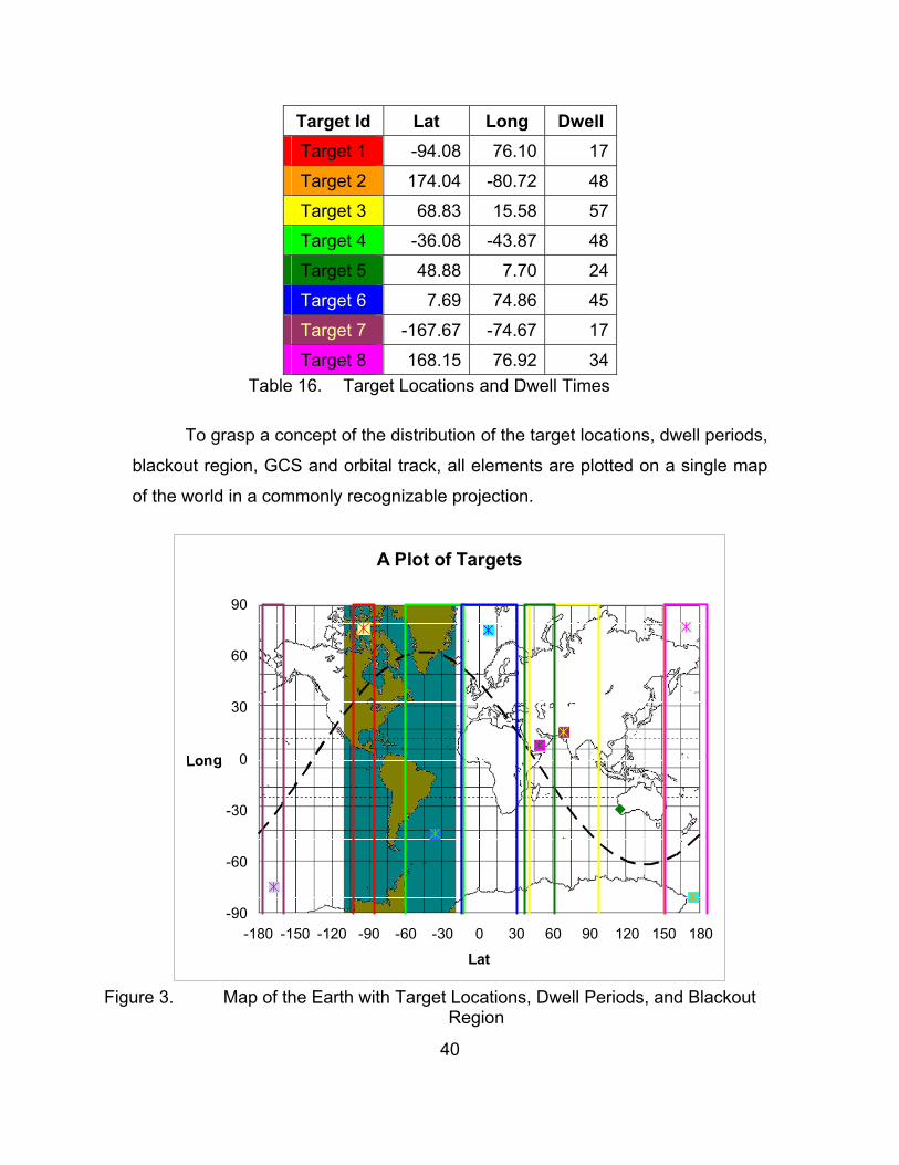
set generation. Table 16 lists a representative version of the data.
40
Target Id Lat Long Dwell Target 1 -94.08 76.10 17
Target 2 174.04 -80.72 48
Target 3 68.83 15.58 57
Target 4 -36.08 -43.87 48
Target 5 48.88 7.70 24
Target 6 7.69 74.86 45
Target 7 -167.67 -74.67 17
Target 8 168.15 76.92 34Table 16. Target Locations and Dwell Times
To grasp a concept of the distribution of the target locations, dwell periods,
blackout region, GCS and orbital track, all elements are plotted on a single map
of the world in a commonly recognizable projection.
A Plot of Targets
-90
-60
-30
0
30
60
90
-180 -150 -120 -90 -60 -30 0 30 60 90 120 150 180
Lat
Long
Figure 3. Map of the Earth with Target Locations, Dwell Periods, and Blackout
Region
41
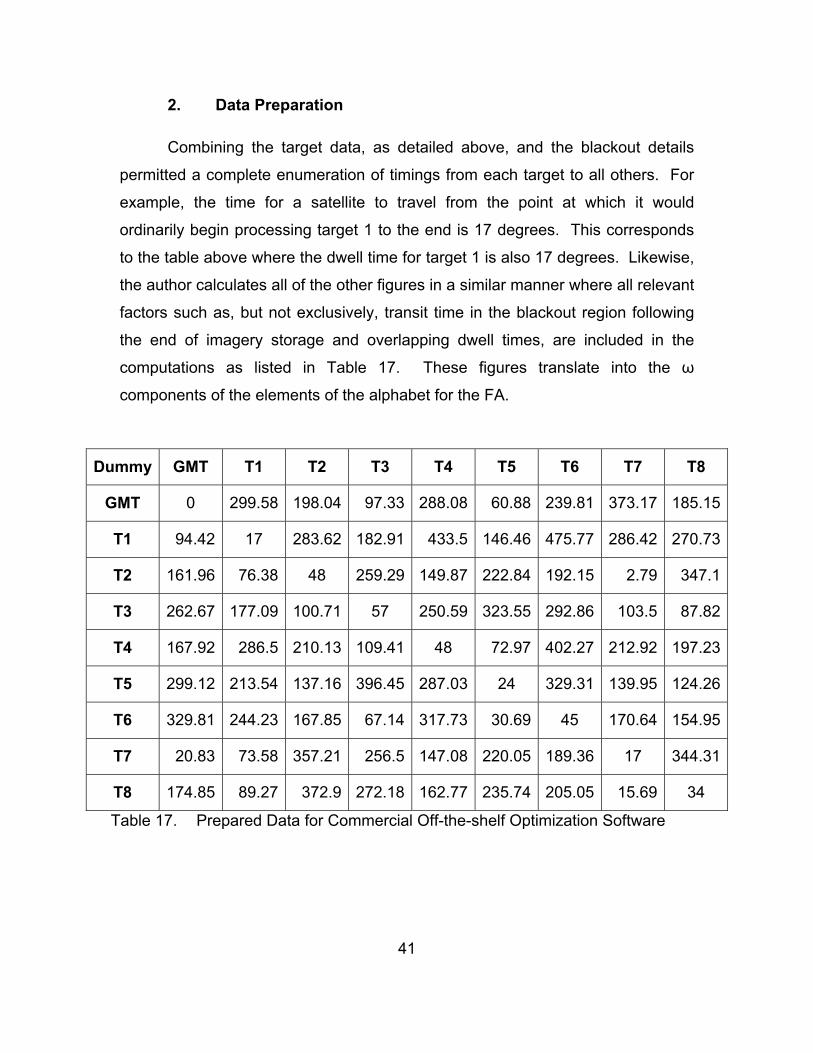
2. Data Preparation
Combining the target data, as detailed above, and the blackout details
permitted a complete enumeration of timings from each target to all others. For
example, the time for a satellite to travel from the point at which it would
ordinarily begin processing target 1 to the end is 17 degrees. This corresponds
to the table above where the dwell time for target 1 is also 17 degrees. Likewise,
the author calculates all of the other figures in a similar manner where all relevant
factors such as, but not exclusively, transit time in the blackout region following
the end of imagery storage and overlapping dwell times, are included in the
computations as listed in Table 17. These figures translate into the ω
components of the elements of the alphabet for the FA.
Dummy GMT T1 T2 T3 T4 T5 T6 T7 T8
GMT 0 299.58 198.04 97.33 288.08 60.88 239.81 373.17 185.15
T1 94.42 17 283.62 182.91 433.5 146.46 475.77 286.42 270.73
T2 161.96 76.38 48 259.29 149.87 222.84 192.15 2.79 347.1
T3 262.67 177.09 100.71 57 250.59 323.55 292.86 103.5 87.82
T4 167.92 286.5 210.13 109.41 48 72.97 402.27 212.92 197.23
T5 299.12 213.54 137.16 396.45 287.03 24 329.31 139.95 124.26
T6 329.81 244.23 167.85 67.14 317.73 30.69 45 170.64 154.95
T7 20.83 73.58 357.21 256.5 147.08 220.05 189.36 17 344.31
T8 174.85 89.27 372.9 272.18 162.77 235.74 205.05 15.69 34
Table 17. Prepared Data for Commercial Off-the-shelf Optimization Software
42
B. FORMULATIONS
Given that the two problems are from related classes of optimization
problems, it is expected that the formulations would be similar – and they are.
However, some subtle differences permit significantly different analyses of the
problem.
1. TSP Formulation
The TSP formulation is:
{ }{ }
, 0, , , 0
1, ,
i j I i j
k K
∈ =
∈
INDICEStarget identifier, including startpoint as
leg identifier
,i jtime i jDATA [UNITS]
duration of leg from to [time]
, ,i j kX
i j k
DECISION VARIABLES [UNITS] a binary varialble with value one only if the satellite
travels from to during leg [dimensionless]
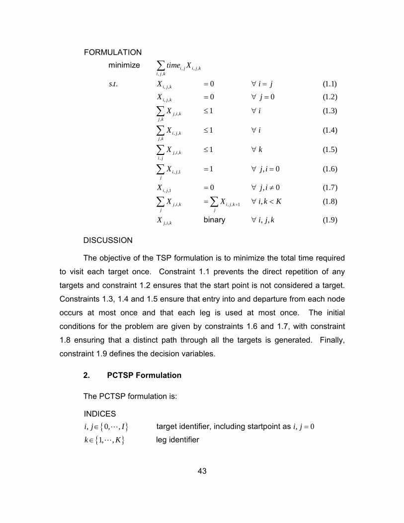
43
, , ,, ,
, ,
, ,
, ,,
, ,,
, ,,
, ,1
, ,1
, , , , 1
. . 0 (1.1)
0 0 (1.2)
1 (1.3)
1 (1.4)
1 (1.5)
1 , 0 (1.6)
0 , 0 (1.7)
, (
i j i j ki j k
i j k
i j k
j i kj k
i j kj k
j i ki j
i jj
i j
j i k i j kj j
time X
s t X i j
X j
X i
X i
X k
X j i
X j i
X X i k K+
= ∀ =
= ∀ =
≤ ∀
≤ ∀
≤ ∀
= ∀ =
= ∀ ≠
= ∀ <
∑
∑
∑
∑
∑
∑ ∑
FORMULATIONminimize
, ,
1.8)
, , (1.9)j i kX i j k∀binary
DISCUSSION
The objective of the TSP formulation is to minimize the total time required
to visit each target once. Constraint 1.1 prevents the direct repetition of any
targets and constraint 1.2 ensures that the start point is not considered a target.
Constraints 1.3, 1.4 and 1.5 ensure that entry into and departure from each node
occurs at most once and that each leg is used at most once. The initial
conditions for the problem are given by constraints 1.6 and 1.7, with constraint
1.8 ensuring that a distinct path through all the targets is generated. Finally,
constraint 1.9 defines the decision variables.
2. PCTSP Formulation
The PCTSP formulation is:
{ }{ }
, 0, , , 0
1, ,
i j I i j
k K
∈ =
∈
INDICEStarget identifier, including startpoint as
leg identifier
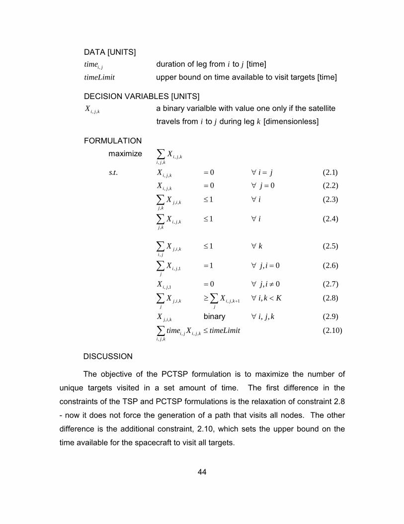
44
,i jtime i j
timeLimit
DATA [UNITS]duration of leg from to [time]upper bound on time available to visit targets [time]
, ,i j kX
i j k
DECISION VARIABLES [UNITS] a binary varialble with value one only if the satellite
travels from to during leg [dimensionless]
, ,, ,
, ,
, ,
, ,,
, ,,
. . 0 (2.1)
0 0 (2.2)
1 (2.3)
1 (2.4)
i j ki j k
i j k
i j k
j i kj k
i j kj k
X
s t X i j
X j
X i
X i
= ∀ =
= ∀ =
≤ ∀
≤ ∀
∑
∑
∑
FORMULATIONmaximize
, ,,
, ,1
, ,1
, , , , 1
, ,
, , ,, ,
1 (2.5)
1 , 0 (2.6)
0 , 0 (2.7)
, (2.8)
, , (2.9)
(2.10)
j i ki j
i jj
i j
j i k i j kj j
j i k
i j i j ki j k
X k
X j i
X j i
X X i k K
X i j k
time X timeLimit
+
≤ ∀
= ∀ =
= ∀ ≠
≥ ∀ <
∀
≤
∑
∑
∑ ∑
∑binary
DISCUSSION
The objective of the PCTSP formulation is to maximize the number of
unique targets visited in a set amount of time. The first difference in the
constraints of the TSP and PCTSP formulations is the relaxation of constraint 2.8
- now it does not force the generation of a path that visits all nodes. The other
difference is the additional constraint, 2.10, which sets the upper bound on the
time available for the spacecraft to visit all targets.
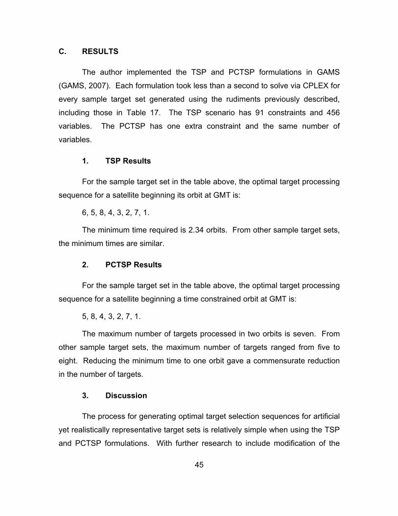
45
C. RESULTS
The author implemented the TSP and PCTSP formulations in GAMS
(GAMS, 2007). Each formulation took less than a second to solve via CPLEX for
every sample target set generated using the rudiments previously described,
including those in Table 17. The TSP scenario has 91 constraints and 456
variables. The PCTSP has one extra constraint and the same number of
variables.
1. TSP Results
For the sample target set in the table above, the optimal target processing
sequence for a satellite beginning its orbit at GMT is:
6, 5, 8, 4, 3, 2, 7, 1.
The minimum time required is 2.34 orbits. From other sample target sets,
the minimum times are similar.
2. PCTSP Results
For the sample target set in the table above, the optimal target processing
sequence for a satellite beginning a time constrained orbit at GMT is:
5, 8, 4, 3, 2, 7, 1.
The maximum number of targets processed in two orbits is seven. From
other sample target sets, the maximum number of targets ranged from five to
eight. Reducing the minimum time to one orbit gave a commensurate reduction
in the number of targets.
3. Discussion
The process for generating optimal target selection sequences for artificial
yet realistically representative target sets is relatively simple when using the TSP
and PCTSP formulations. With further research to include modification of the
46
GAMS code and the input data files it is possible generate all the FA inputs, in
the correct sequence, for the entire mission as part of the optimization procedure.
Additional research and analysis is required to determine how or even if these or
equivalent formulations or processes could be achieved using just the elements
of the FA.
47
V. CONCLUSION AND RECOMMENDATIONS
A. CONCLUSION
Satellite systems can indeed be modeled using FA. It is considered that
the fidelity of the models produced in the thesis is sufficient, yet for more in-depth
research additional detailed models are needed to provide a wider scope for
analysis and exploration of the field. Regardless, the benefits of FA are that they
are simple without being simplistic yet at the same time permit a wide variety of
factors to be included in the model. In order to effectively construct an FA, there
is a considerable amount of knowledge of the system to be modeled that must be
brought together and understood. In particular, the state space, transition
function and language need clear and unambiguous definitions. For the multiple
spacecraft system the task becomes more complex as various interactions also
need to be either permitted and expressible or prohibited by the model.
However, by using clearly defined specific assumptions and indicative
values these preliminary models maintain tractability. Additionally, there is a very
broad foundation from which to pursue further analysis and development of the
models in the thesis. The exploration of the growth of more complex models and
optimization classifications beyond the TSP and the PCTSP formulations are
indicative of some areas for further research.
B. RECOMMENDATIONS
In terms of the research done in this thesis and the concluding comments,
the author presents the following recommendations for further research and
analysis. The application of FA to other problems is also acknowledged as a
worthy endeavor.
48
1. Graphical Representations
A graphical representation of an FA often provides insight to the reader
that is not normally evident via an equivalent cursory reading of the details and
specifications of the FA. Taking the two FA described herein and constructing a
graphical representation could very well highlight additional aspects of the
multiple satellite system that are not presently obvious. It is recommended that
any extension of this research commence with the production of graphical
representations of the FA presented herein.
2. More Spacecraft in the Model
The addition of more spacecraft to the model would increase the realism
and complexity of the FA. In addition, with the appropriate management of the
state space and other elements of the FA the model could be developed along a
similar process used for this problem. A constellation of about five spacecraft
would represent a suitable system. Special attention is needed for the
construction and clarification of joint tasks. It is recommended that additional
spacecraft be added to this model along with the production of explicit
instructions, rule sets or constraints to govern the generation, proliferation and
management of joint tasks (Kang, Sparks & Banda, 2000 & 2001).
3. NFA
Beyond the additional spacecraft, an application of NFA or possibly even
the development of a collection of smaller FA could also prove useful in modeling
the various failure modalities faced by satellite systems. This could also be
combined with some stochastic Markovian analysis and modeling. It is
recommended that extensions of this research that investigate the effects of
failures on the optimization of tasking and scheduling encompass a combination
of stochastic Markovian procedures and NFA.
49
4. PDA
In progressing to a “smart” satellite system where the individual spacecraft
have the capability for task storage and retrieval and other functions, there is
scope for the employment of PDA. It is recommended that this be investigated
as an individual problem or in concert with the others describe above.
5. Integer Linear Programming (ILP) Relationship to FA
Finally, given a functional FA, as arisen from the recommendations above,
it requires a much more thorough and in-depth analysis of the processes to
transform the FA into an ILP and the relationships between the two constructs
than that delivered by this thesis. This could address such issues as the
developing of heuristics or other novel solutions to resolving conflicting tasking
and scheduling of multiple satellite systems. It is recommended that a
comprehensive examination of the processes and procedures to transform an FA
into an ILP and the relationships between the two constructs be undertaken.
Additionally, it is recommended that the modification of the commercial off-the-
shelf optimization software input files be explored so that its output would also
generate all the FA inputs, in the correct sequence, for the entire optimized
mission (Kam, 1996; Kang & Sparks, 2003).

50
THIS PAGE INTENTIONALLY LEFT BLANK
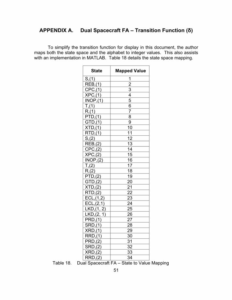
51
APPENDIX A. Dual Spacecraft FA – Transition Function (δ)
To simplify the transition function for display in this document, the author maps both the state space and the alphabet to integer values. This also assists with an implementation in MATLAB. Table 18 details the state space mapping.
State Mapped Value
S,(1) 1 REB,(1) 2 CPC,(1) 3 XPC,(1) 4 INOP,(1) 5 T,(1) 6 R,(1) 7 PTD,(1) 8 GTD,(1) 9 XTD,(1) 10 RTD,(1) 11 S,(2) 12 REB,(2) 13 CPC,(2) 14 XPC,(2) 15 INOP,(2) 16 T,(2) 17 R,(2) 18 PTD,(2) 19 GTD,(2) 20 XTD,(2) 21 RTD,(2) 22 ECL,(1,2) 23 ECL,(2,1) 24 LKD,(1, 2) 25 LKD,(2, 1) 26 PRD,(1) 27 SRD,(1) 28 XRD,(1) 29 RRD,(1) 30 PRD,(2) 31 SRD,(2) 32 XRD,(2) 33 RRD,(2) 34
Table 18. Dual Spacecraft FA – State to Value Mapping
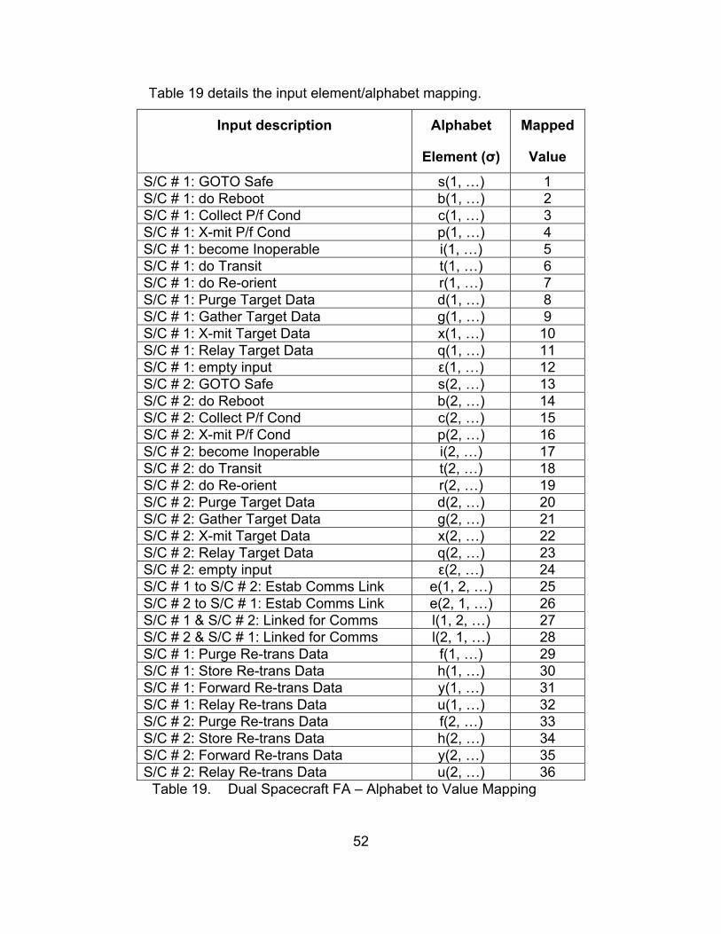
52
Table 19 details the input element/alphabet mapping.
Input description Alphabet
Element (σ)
Mapped
Value
S/C # 1: GOTO Safe s(1, …) 1 S/C # 1: do Reboot b(1, …) 2 S/C # 1: Collect P/f Cond c(1, …) 3 S/C # 1: X-mit P/f Cond p(1, …) 4 S/C # 1: become Inoperable i(1, …) 5 S/C # 1: do Transit t(1, …) 6 S/C # 1: do Re-orient r(1, …) 7 S/C # 1: Purge Target Data d(1, …) 8 S/C # 1: Gather Target Data g(1, …) 9 S/C # 1: X-mit Target Data x(1, …) 10 S/C # 1: Relay Target Data q(1, …) 11 S/C # 1: empty input ε(1, …) 12 S/C # 2: GOTO Safe s(2, …) 13 S/C # 2: do Reboot b(2, …) 14 S/C # 2: Collect P/f Cond c(2, …) 15 S/C # 2: X-mit P/f Cond p(2, …) 16 S/C # 2: become Inoperable i(2, …) 17 S/C # 2: do Transit t(2, …) 18 S/C # 2: do Re-orient r(2, …) 19 S/C # 2: Purge Target Data d(2, …) 20 S/C # 2: Gather Target Data g(2, …) 21 S/C # 2: X-mit Target Data x(2, …) 22 S/C # 2: Relay Target Data q(2, …) 23 S/C # 2: empty input ε(2, …) 24 S/C # 1 to S/C # 2: Estab Comms Link e(1, 2, …) 25 S/C # 2 to S/C # 1: Estab Comms Link e(2, 1, …) 26 S/C # 1 & S/C # 2: Linked for Comms l(1, 2, …) 27 S/C # 2 & S/C # 1: Linked for Comms l(2, 1, …) 28 S/C # 1: Purge Re-trans Data f(1, …) 29 S/C # 1: Store Re-trans Data h(1, …) 30 S/C # 1: Forward Re-trans Data y(1, …) 31 S/C # 1: Relay Re-trans Data u(1, …) 32 S/C # 2: Purge Re-trans Data f(2, …) 33 S/C # 2: Store Re-trans Data h(2, …) 34 S/C # 2: Forward Re-trans Data y(2, …) 35 S/C # 2: Relay Re-trans Data u(2, …) 36
Table 19. Dual Spacecraft FA – Alphabet to Value Mapping
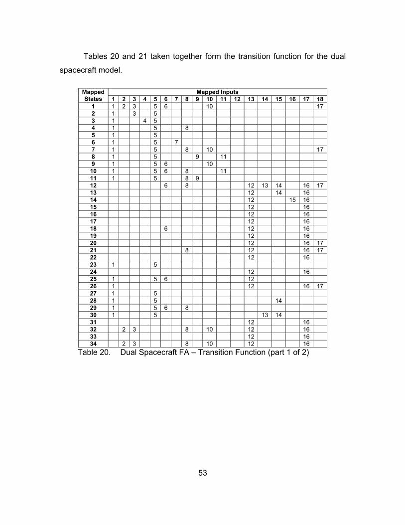
53
Tables 20 and 21 taken together form the transition function for the dual
spacecraft model.
Mapped Inputs Mapped
States 1 2 3 4 5 6 7 8 9 10 11 12 13 14 15 16 17 18 1 1 2 3 5 6 10 17 2 1 3 5 3 1 4 5 4 1 5 8 5 1 5 6 1 5 7 7 1 5 8 10 17 8 1 5 9 11 9 1 5 6 10 10 1 5 6 8 11 11 1 5 8 9 12 6 8 12 13 14 16 17 13 12 14 16 14 12 15 16 15 12 16 16 12 16 17 12 16 18 6 12 16 19 12 16 20 12 16 17 21 8 12 16 17 22 12 16 23 1 5 24 12 16 25 1 5 6 12 26 1 12 16 17 27 1 5 28 1 5 14 29 1 5 6 8 30 1 5 13 14 31 12 16 32 2 3 8 10 12 16 33 12 16 34 2 3 8 10 12 16
Table 20. Dual Spacecraft FA – Transition Function (part 1 of 2)
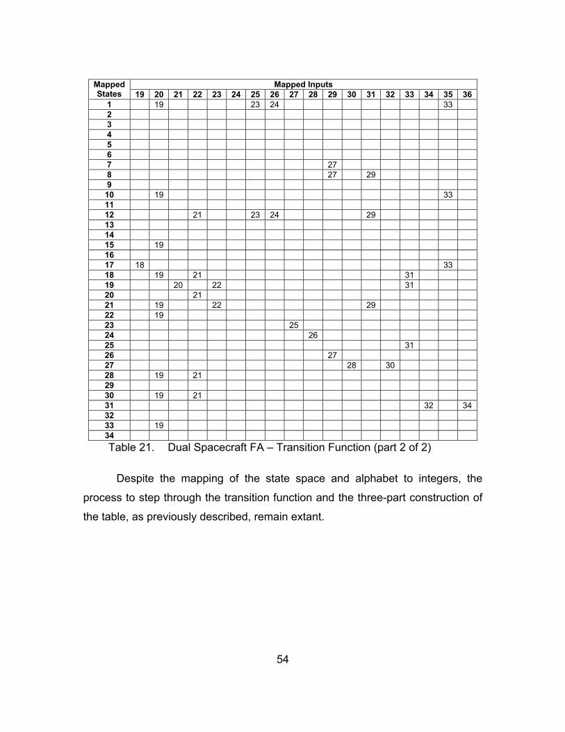
54
Mapped Inputs Mapped
States 19 20 21 22 23 24 25 26 27 28 29 30 31 32 33 34 35 36 1 19 23 24 33 2 3 4 5 6 7 27 8 27 29 9 10 19 33 11 12 21 23 24 29 13 14 15 19 16 17 18 33 18 19 21 31 19 20 22 31 20 21 21 19 22 29 22 19 23 25 24 26 25 31 26 27 27 28 30 28 19 21 29 30 19 21 31 32 34 32 33 19 34 Table 21. Dual Spacecraft FA – Transition Function (part 2 of 2)
Despite the mapping of the state space and alphabet to integers, the
process to step through the transition function and the three-part construction of
the table, as previously described, remain extant.
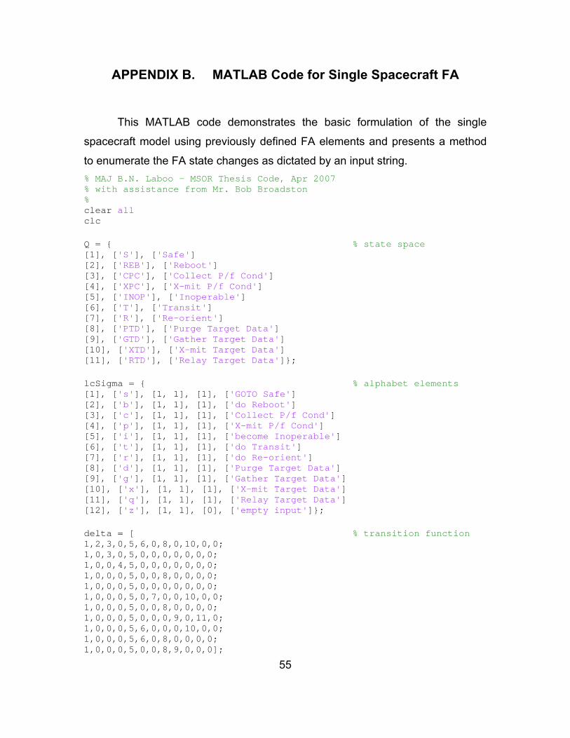
55
APPENDIX B. MATLAB Code for Single Spacecraft FA
This MATLAB code demonstrates the basic formulation of the single
spacecraft model using previously defined FA elements and presents a method
to enumerate the FA state changes as dictated by an input string. % MAJ B.N. Laboo - MSOR Thesis Code, Apr 2007 % with assistance from Mr. Bob Broadston % clear all clc Q = { % state space [1], ['S'], ['Safe'] [2], ['REB'], ['Reboot'] [3], ['CPC'], ['Collect P/f Cond'] [4], ['XPC'], ['X-mit P/f Cond'] [5], ['INOP'], ['Inoperable'] [6], ['T'], ['Transit'] [7], ['R'], ['Re-orient'] [8], ['PTD'], ['Purge Target Data'] [9], ['GTD'], ['Gather Target Data'] [10], ['XTD'], ['X-mit Target Data'] [11], ['RTD'], ['Relay Target Data']}; lcSigma = { % alphabet elements [1], ['s'], [1, 1], [1], ['GOTO Safe'] [2], ['b'], [1, 1], [1], ['do Reboot'] [3], ['c'], [1, 1], [1], ['Collect P/f Cond'] [4], ['p'], [1, 1], [1], ['X-mit P/f Cond'] [5], ['i'], [1, 1], [1], ['become Inoperable'] [6], ['t'], [1, 1], [1], ['do Transit'] [7], ['r'], [1, 1], [1], ['do Re-orient'] [8], ['d'], [1, 1], [1], ['Purge Target Data'] [9], ['g'], [1, 1], [1], ['Gather Target Data'] [10], ['x'], [1, 1], [1], ['X-mit Target Data'] [11], ['q'], [1, 1], [1], ['Relay Target Data'] [12], ['z'], [1, 1], [0], ['empty input']}; delta = [ % transition function 1,2,3,0,5,6,0,8,0,10,0,0; 1,0,3,0,5,0,0,0,0,0,0,0; 1,0,0,4,5,0,0,0,0,0,0,0; 1,0,0,0,5,0,0,8,0,0,0,0; 1,0,0,0,5,0,0,0,0,0,0,0; 1,0,0,0,5,0,7,0,0,10,0,0; 1,0,0,0,5,0,0,8,0,0,0,0; 1,0,0,0,5,0,0,0,9,0,11,0; 1,0,0,0,5,6,0,0,0,10,0,0; 1,0,0,0,5,6,0,8,0,0,0,0; 1,0,0,0,5,0,0,8,9,0,0,0];
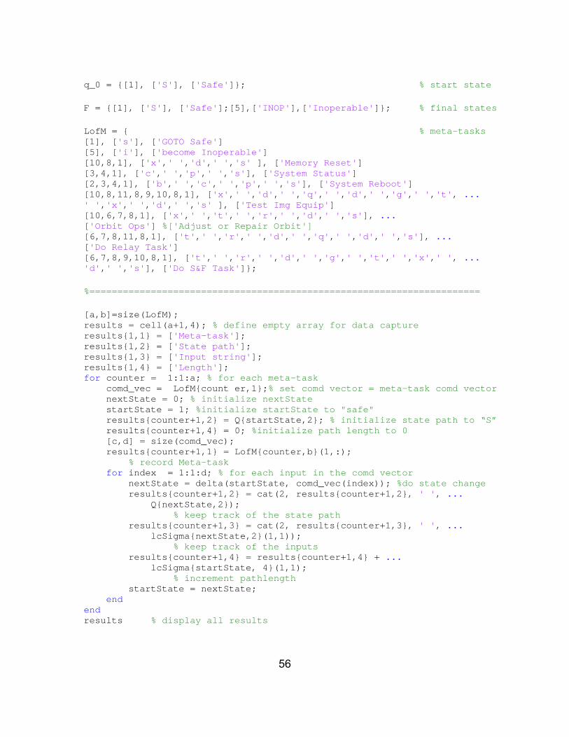
56
q_0 = {[1], ['S'], ['Safe']}; % start state F = {[1], ['S'], ['Safe'];[5],['INOP'],['Inoperable']}; % final states LofM = { % meta-tasks [1], ['s'], ['GOTO Safe'] [5], ['i'], ['become Inoperable'] [10,8,1], ['x',' ','d',' ','s' ], ['Memory Reset'] [3,4,1], ['c',' ','p',' ','s'], ['System Status'] [2,3,4,1], ['b',' ','c',' ','p',' ','s'], ['System Reboot'] [10,8,11,8,9,10,8,1], ['x',' ','d',' ','q',' ','d',' ','g',' ','t', ... ' ','x',' ','d',' ','s' ], ['Test Img Equip'] [10,6,7,8,1], ['x',' ','t',' ','r',' ','d',' ','s'], ... ['Orbit Ops'] %['Adjust or Repair Orbit'] [6,7,8,11,8,1], ['t',' ','r',' ','d',' ','q',' ','d',' ','s'], ... ['Do Relay Task'] [6,7,8,9,10,8,1], ['t',' ','r',' ','d',' ','g',' ','t',' ','x',' ', ... 'd',' ','s'], ['Do S&F Task']}; %====================================================================== [a,b]=size(LofM); results = cell(a+1,4); % define empty array for data capture results{1,1} = ['Meta-task']; results{1,2} = ['State path']; results{1,3} = ['Input string']; results{1,4} = ['Length']; for counter = 1:1:a; % for each meta-task comd_vec = LofM{count er,1};% set comd vector = meta-task comd vector nextState = 0; % initialize nextState startState = 1; %initialize startState to "safe" results{counter+1,2} = Q{startState,2}; % initialize state path to “S” results{counter+1,4} = 0; %initialize path length to 0 [c,d] = size(comd_vec); results{counter+1,1} = LofM{counter,b}(1,:); % record Meta-task for index = 1:1:d; % for each input in the comd vector nextState = delta(startState, comd_vec(index)); %do state change results{counter+1,2} = cat(2, results{counter+1,2}, ' ', ... Q{nextState,2}); % keep track of the state path results{counter+1,3} = cat(2, results{counter+1,3}, ' ', ... lcSigma{nextState,2}(1,1)); % keep track of the inputs results{counter+1,4} = results{counter+1,4} + ... lcSigma{startState, 4}(1,1); % increment pathlength startState = nextState; end end results % display all results
57
LIST OF REFERENCES
Avanzini, Giulio, Davide Biamonti and Edmondo A. Minisci. 2004. Minimum-Fuel/Minimum-time maneuvers of formation flying satellites. Advances in the Astronautical Sciences 116, (Suppl.) (Advances in the Astronautical Sciences. Vol. 116, Suppl., pp. 1-20.): 1-20.
Boddy, Mark S., Steven A. Harp and Kyle S. Nelson. 2004. CLOCKWORK: Requirements Definition and Technology Evaluation for Robust, Compiled Autonomous Spacecraft. NASA NAG-2-1634, 15 January 2004.
Broadston, R. 2007. Department of Electrical & Computer Engineering, Senior Lecturer, Personal dialogue April 2007.
Carlyle, M. 2006. NPS Department of Operations Research, Assoc Prof. of Operation Research, Personal dialogue July 2006.
Carrasco, Rafael C., and José Oncina. 1994. Learning stochastic regular grammars by means of a state merging method. Paper presented at ICGI '94: Proceedings of the Second International Colloquium on Grammatical Inference and Applications.
Cassandras, Christos G., and Stéphane Lafortune. 1999. Introduction to discrete event systems. Kluwer international series on discrete event dynamic systems. Boston: Kluwer Academic.
Chan, Wai Kin (Victor). 2005. Mathematical programming representations of discrete-event system dynamics. PhD diss, UCB.
Chan, Wai Kin (Victor), and Lee W. Schruben. 2003. Properties of discrete event systems from their mathematical programming representations. 2003. Proceedings of the 2003 Winter Simulation Conference, 2003, 1, 496-502 Vol. 1.
Chan, Wai Kin (Victor), and Lee W. Schruben. 2004. Generating scheduling constraints for discrete event dynamic systems. Paper presented at WSC '04: Proceedings of the 36th conference on Winter simulation, Washington, D.C.
Chan, Wai Kin (Victor), and Lee W. Schruben. 2006. Response gradient estimation using mathematical programming models of discrete-event system sample paths. Paper presented at WSC '06: Proceedings of the 38th conference on Winter simulation, Monterey, California.
58
Chaves, Antonio Augusto, and Luiz Antonio Nogueira Lorena. 2005. Hybrid algorithms with detection of promising areas for the prize collecting traveling salesman problem. Paper presented at HIS '05: Proceedings of the Fifth International Conference on Hybrid Intelligent Systems.
Chien, Steve, Rob Sherwood, Michael Burl, Russell Knight, Gregg Rabideau, Barbara Engelhardt, Ashley Davies, Paul Zetocha, Ross Wainwright, Pete Klupar, Pat Cappelaere, Derek Surka, Brian Williams, Ronald Greeley, Victor Baker, James Doan. 2001. The Techsat-21 Autonomous Sciencecraft Constellation. Jet Propulsion Laboratory, California Institute of Technology.
Cobleigh, J. M., Clarke, L. A., and Osterweil L. J. 2002. FLAVERS: A finite state verification technique for software systems. IBM SYSTEMS JOURNAL, Vol. 41, No. 1, 140–165.
Damiani, M. 1997. The state reduction of nondeterministic finite-state machines. Computer-Aided Design of Integrated Circuits and Systems, IEEE Transactions on 16, (11): 1278-1291.
Dantzig, G. B., R. Fulkerson, and, S. M. Johnson. 1954. Solution of a large-scale traveling salesman problem. Operations Research 2, 393-410.
Department of the Army. 2005. Field Manual No. 3-14: Space Support to Army Operations. Headquarters, Department of the Army. Washington, DC, 18 May 2005.
Department of the Army. 2006. TRADOC Pamphlet 525-7-4 Military Operations Army Space Operations Concept Capability Plan. Headquarters, United States Army Training and Doctrine Command Fort Monroe, Virginia 23651-1047 15 November 2006.
Frank, A., 2005, Finite-State Automata and Algorithms, Computational Linguistics, Vorlesung: Computerlinguistik, 2. Studienabschnitt, April 25, http://www.coli.uni-saarland.de/~frank/contents/slides/fsa.pdf. Last Accessed June 2007.
Frasconi, Paolo, Marco Gori, Marco Maggini, and Giovanni Soda. 1996. Representation of finite state automata in recurrent radial basis function networks. Machine Learning 23, (1): 5-32.
GAMS. 2007. http://www.gams.com, v2.0.34.19. June 4, 2007. Last Accessed June 2007.
Gutin, G. and A. P. Punnen. 2006. The Traveling Salesman Problem and Its Variations. Springer.
59
Harel, David. 1987. Statecharts: A visual formalism for Complex systems. Science of Computer Programming 8 (1987) 231-274. North-Holland.
Hennie, Frederick C. 1968. Finite-state models for logical machines. New York: Wiley.
Hopcroft, John E., and Jeffrey D. Ullman. 1979. Introduction to automata theory, languages, and computation. Addison-Wesley series in computer science. Reading, MA: Addison-Wesley.
Hopcroft, John E., and Jeffrey D. Ullman. 1969. Formal languages and their relation to automata. Addison-Wesley series in computer science and information processing. Reading, MA: Addison-Wesley Pub. Co.
Horning, James (Jim), NPS Department of Space Systems, Research Associate, Personal dialogue July/August 2006.
Hunt, D'Hania J. 2002. Constructing higher-order de bruijn graphs. MS Thesis, NPS.
Joly, Charles Jasper. 1905. "A manual of Quaternions". London, Macmillan and co., limited; New York, The Macmillan Company, 1905. LCCN 05036137.
Kam, Timothy. 1996. Synthesis of finite state machines: Functional optimization. Boston, MA: Kluwer Academic Publishers.
Kan, Shirley, April 23, 2007, CRS Report for Congress (RS22652) - China’s Anti-Satellite Weapon Test.
Kang, Wei, and Andy Sparks. 2003. Modeling and computation of optimal task assignment for cooperative control. Proceedings of 42nd IEEE Conference on Decision and Control, 2003, 1, 1017-1022 Vol. 1.
Kang, Wei, Andy Sparks, and Siva Banda. 2000. Multi-satellite formation and reconfiguration. Paper presented at 2000 American Control Conference, Chicago, IL; UNITED STATES; 28-30 June 2000.
Kang, Wei, Andy Sparks, and Siva Banda. 2001. Coordinated control of multi-satellite systems. Journal of Guidance 24, (2) (Journal of Guidance, Control, and Dynamics. Vol. 24, no. 2, pp. 360-368. March-April): 360-368.
Kuipers, Jack B. 1999. Quaternions and rotation sequences: A primer with applications to orbits, aerospace, and virtual reality. Princeton, NJ: Princeton University Press.
60
Lawler, E. L. (ed.); Lenstra, J. K. (ed.); Rinnooy Kan, A. H. G.(ed.); Shmoys, D. B. (ed.). 1985. The traveling salesman problem: A guided tour of combinatorial optimization. Wiley-Interscience Series in Discrete Mathematics. A Wiley-Interscience publication. Chichester etc. John Wiley & Sons.
MATLAB. 2007. http://www.mathworks.com/R2007a. March 1 2007, Last Accessed June 2007.
McCullough, B. D., and Berry Wilson. 1999. On the accuracy of statistical procedures in Microsoft Excel 97. Computational Statistics & Data Analysis 31, (1): 27-37. July 28.
McCullough, B. D., and Berry Wilson. 2002. On the accuracy of statistical procedures in Microsoft Excel 2000 and Excel XP. Computational Statistics & Data Analysis 40, (4): 713-721. October 28.
McCullough, B. D., and Berry Wilson. 2005. On the accuracy of statistical procedures in Microsoft Excel 2003. Computational Statistics & Data Analysis 49, (4): 1244-1252. June 15.
Meshishnek, M. J. 1995. Aerospace Report No. TR-95(5231)-3: Overview of the Space Debris Environment. Mechanics and Materials Technology Center, Technology Operations. Space and Missile Systems Center, Air Force Materiel Command. Los Angeles Air Force Base, CA 90245.
Moscinski, Jerzy, and Zbigniew Ogonowski. 1995. Advanced control with MATLAB and SIMULINK. London; New York: Ellis Horwood.
Nelson, B. 2007. Australia-US Joint Communications Facility to be Hosted at Geraldton, Department of Defence (Australia) Media release 007, February 15.
Pisacane, Vincent L. 1994. Fundamentals of space systems. The Johns Hopkins University/Applied physics laboratory series in science and engineering. Oxford; New York: Oxford University Press.
Pisacane, Vincent L. 2005. Fundamentals of space systems. The Johns Hopkins University/Applied physics laboratory series in science and engineering. 2nd ed. Oxford; New York: Oxford University Press.
Radivojevic, I. and F. Brewer. 1994. Ensemble representation and techniques for exact control-dependent scheduling.
Ross, Alan and Prof. Herschel Loomis. 2007. NPS Department of Electrical and Computer Engineering & Space Systems Academic Group, Personal dialogue April/May 2007.
61
Ross, Prof. I. Mike. 2006-7. NPS Department of Mechanical and Astronautical Engineering, Personal dialogue 2006-7.
Ross, Sheldon M. 2003. Introduction to probability models. 8th ed. San Diego, CA: Academic Press.
Sanchez, P., 2006. NPS Department of Operations Research, Senior Lecturer, Personal dialogue, December 5, 2006.
Satnews Daily. 2007. U.S. Denies Destroying Russian Satellite, Satnews Daily, April 6, http://www.satnews.com/stories2007/4247/. Last Accessed June 2007.
SEC (Space Environment Center). 2007. Space Environment Center Topic Paper: Satellites and Space Weather. http://www.sec.noaa.gov/info/Satellites.html. April 16, 2007. Last Accessed June 2007.
Sekhavat, P. 2007. NPS Department of Mechanical and Astronautical Engineering, Post-Doc Research Associate, Personal dialogue January 2007.
Tomme, Edward B. 2006. The myth of the tactical satellite. Air & Space Power Journal 20, (2) (Summer): 89.
Tung, B., and L. Kleinrock. 1996. Using finite state automata to produce self-optimization and self-control. Parallel and Distributed Systems, IEEE Transactions on 7, (4): 439-448.
Volpano, Dennis M. 2007. NPS Department of Computer Science, Associate Prof, Personal dialogue, February/March 2007.
Wikipedia, Orbit. 2007. http://en.wikipedia.org/wiki/Orbit, February 5, 2007. Last Accessed June 2007.
Wilson, Tom. 2001. Threats to United States Space Capabilities. Space Commission Staff Member, Prepared for the Commission to Assess United States National Security. Space Management and Organization, Washington, DC.
Wu, Tzu-li. 1992. Optimization models for underway replenishment of a dispersed carrier battle group. MS Thesis, NPS.
Yang, J. C. -Y, G. de Micheli, and M. Damiani. 1996. Scheduling and control generation with environmental constraints based on automata representations. Computer-Aided Design of Integrated Circuits and Systems, IEEE Transactions on 15, (2): 166-183.

62
THIS PAGE INTENTIONALLY LEFT BLANK
63
INITIAL DISTRIBUTION LIST
1. Defense Technical Information Center Ft. Belvoir, Virginia
2. Dudley Knox Library Naval Postgraduate School Monterey, California
3. Career Advisor Health Services (for member’s file) Directorate of Officer Career Management Canberra, Australian Capital Territory (Australia)
4. DSTO Research Library Edinburgh Defence Science and Technology Organisation Edinburgh, South Australia (Australia)
5. Professor Robert F. Dell Naval Postgraduate School Monterey, California
6. Professor I. Mike. Ross Naval Postgraduate School Monterey, California
7. Prof Wei Kang Naval Postgraduate School Monterey, California
8. Professor Bill Gragg Naval Postgraduate School Monterey, California
9. Professor Hal Fredricksen Naval Postgraduate School Monterey, California
10. Professor Herschel H. Loomis Jr. Naval Postgraduate School Monterey, California
11. Professor Alan Ross Naval Postgraduate School Monterey, California
64
12. Emeritus Professor Neville de Mestre
Bond University Gold Coast, Queensland (Australia)
13. Lady Karen Carolyn Nimmo Royal College of Advanced Research of the Principality of Hutt River Hutt River, Principality of Hutt River
14. Ken Kranz Alternative Science & Technology Research Organisation Sheidow Park, South Australia (Australia)
15. Professor John R.R. Searl Direct International Science Consortium, Inc Rochester, New York
16. Carol Laboo Wishart, Queensland (Australia)
17. Brett Laboo C/- Australian Embassy Washington, DC


