
NBER WORKING PAPER SERIES
INVESTMENT UNDER UNCERTAINTYAND TIME-INCONSISTENT PREFERENCES
Steven R. GrenadierNeng Wang
Working Paper 12042http://www.nber.org/papers/w12042
NATIONAL BUREAU OF ECONOMIC RESEARCH1050 Massachusetts Avenue
Cambridge, MA 02138February 2006
We thank Christopher Harris, Gur Huberman, David Laibson, Ulrike Malmendier, Chris Mayer, BobMcDonald, Tano Santos, Tom Sargent, Mike Woodford, Wei Xiong, the anonymous referee, and seminarparticipants at Columbia, NYU, and Wisconsin (Madison) for helpful comments. The views expressed hereinare those of the author(s) and do not necessarily reflect the views of the National Bureau of EconomicResearch.
©2006 by Steven R. Grenadier and Neng Wang. All rights reserved. Short sections of text, not to exceedtwo paragraphs, may be quoted without explicit permission provided that full credit, including © notice, isgiven to the source.

Investment Under Uncertainty and Time-Inconsistent PreferencesSteven R. Grenadier and Neng WangNBER Working Paper No. 12042February 2006JEL No. G11, G31, D9
ABSTRACT
The real options framework has been used extensively to analyze the timing of investment under
uncertainty. While standard real options models assume that agents possess a constant rate of time
preference, there is substantial evidence that agents are very impatient about choices in the short-
term, but are quite patient when choosing between long-term alternatives. We extend the real options
framework to model the investment timing decisions of entrepreneurs with such time-inconsistent
preferences. Two opposing forces determine investment timing: while evolving uncertainty induces
entrepreneurs to defer investment in order to take advantage of the option to wait, their time-
inconsistent preferences motivate them to invest earlier in order to avoid the time-inconsistent
behavior they will display in the future. We find that the precise trade-off between these two forces
depends on such factors as whether entrepreneurs are sophisticated or naive in their expectations
regarding their future time-inconsistent behavior, as well as whether the payoff from investment
occurs all at once or over time. We extend the model to consider equilibrium investment behavior
for an industry comprised of time-inconsistent entrepreneurs. Such an equilibrium involves the dual
problem of entrepreneurs playing dynamic games against competitors as well as against their own
future selves.
Steven R. GrenadierGraduate School of BusinessStanford UniversityStanford, CA 94305and [email protected]
Neng WangColumbia Business School3022 BroadwayUris Hall 812New York, NY [email protected]
1 Introduction
Since the seminal work of Brennan and Schwartz (1985) and McDonald and Siegel (1986), the
real options approach to investment under uncertainty has become an essential part of modern
economics and finance.1 In this paper, we consider a particularly well-suited application of the
real options framework: the investment decision of an entrepreneur. The skills, experience
and luck of the entrepreneur have endowed him with an investment opportunity in a risky
project.2 Essentially, the real options approach posits that the opportunity to invest in a
project is analogous to an American call option on the investment project. Thus, the timing
of investment is economically equivalent to the optimal exercise decision for an option.
In the standard real options framework it is assumed that agents have a constant rate
of time preference. Thus real options models typically assume that rewards are discounted
exponentially. Such preferences are time-consistent in that an entrepreneur’s preference for
rewards at an earlier date over a later date is the same no matter when he is asked. However,
virtually every experimental study on time preferences suggests that the assumption of time-
consistency is unrealistic.3 When two rewards are both far away in time, decision makers
act relatively patiently (e.g., they prefer two apples in 101 days, rather than one apple in
100 days). But when both rewards are brought forward in time, decision makers act more
impatiently (e.g., they prefer one apple today, rather than two apples tomorrow). Laib-
son (1997) models such time-varying impatience with quasi-hyperbolic discount functions,
where the discount rate declines as the horizon increases.4 Such preferences are also termed
“present-biased” preferences by O’Donoghue and Rabin (1999a).1The application of the real options approach to investment is quite broad. Brennan and Schwartz (1985)
use an option pricing approach to analyze investment in natural resources. McDonald and Siegel (1986)provided the standard continuous-time framework for analysis of a firm’s investment in a single project. Majdand Pindyck (1987) enrich the analysis with a time-to-build feature. Dixit (1989) uses the real option approachto examine entry and exit from a productive activity. Titman (1985) and Williams (1991) use the real optionsapproach to analyze real estate development. Grenadier (1996, 2002) and Lambrecht and Perraudin (2003)extend real options to a game-theoretic environment.
2We assume that this investment option is non-tradable and its payoff cannot be spanned by existing assets.The lack of tradability is important to our model, since we wish to rule out time-inconsistent entrepreneursselling their investment options to time-consistent entrepreneurs. Lack of tradability could be caused by theoption’s value emanating from the special skills of the entrepreneur or to asymmetric information resultingin a “lemons” problem. The fact the option is non-tradable and is not spanned by existing assets impliesthat the entrepreneur will use a “private” discount rate, reflecting his subjective valuation of cash flows. SeeChapter 4 of Dixit and Pindyck (1994) for a more complete discussion of subjective discount rates wherespanning does not exist.
3For example, see Thaler (1981), Ainslie (1992) and Loewenstein and Prelec (1992).4Applications of quasi-hyperbolic preferences are now quite extensive. For some examples, see Barro (1999)
for an application to the neoclassical growth model, O’Donoghue and Rabin (1999b) for a principal agentmodel, DellaVigna and Malmendier (2004) for contract design between firms and consumers, and Luttmerand Mariotti (2003) for asset pricing in an exchange economy.
1
This paper merges two important strands of research: the real options approach that
emphasizes the benefits of waiting to invest in an uncertain environment, and the literature
on hyperbolic preferences where decision makers face the difficult problem of making optimal
choices in a time-inconsistent framework.5 On the one hand, standard real options models
imply a large option value of waiting: typical parameterizations in the literature show that
investment should not occur until the payoff is at least double the cost. On the other hand,
time-inconsistent preferences provide an incentive to hurry investment in order to avoid sub-
optimal decisions made in the future. Our model can show precisely how these two opposing
forces interact.6
We find it reasonable to believe that entrepreneurs (such as an individual or a small
private partnership) are more prone to time-inconsistent behavior than firms. Consistent
with this, Brocas and Carrillo (2004) assume that entrepreneurs have hyperbolic preferences.
Similarly, DellaVigna and Malmendier (2004) assume that individuals are time-inconsistent,
but that firms (with whom the individuals contract) are rational and time-consistent. Pre-
sumably there is something about the organization of a firm and its delegated, professional
management that mitigates or removes the time-inconsistency from the firm’s decisions. Of
course, little research has been done to precisely identify which individuals or institutions are
more prone to time-inconsistency. The classic real option example of commercial real es-
tate development may be particularly apt for this entrepreneurial setting. The development
of commercial real estate is analogous to an American call option on a building, where the
exercise price is equal to the construction cost. Williams (2001) states that land (both im-
proved and unimproved) is primarily held and developed by noninstitutional investors (such
as individuals and private partnerships), rather than by institutional investors. Such devel-
opers are often termed “merchant builders” who construct buildings (generally standardized,
conventional properties) and then sell them to institutional investors.
As is standard in models of time-inconsistent decision making, such problems are envi-
sioned as the outcome of an “intra-personal game” in which the same individual entrepreneur5While we are assuming that entrepreneurs apply hyperbolic discounting to cash flows, nothing substantive
would change if we instead assumed that entrepreneurs applied hyperbolic discounting to consumption, butwhere the entrepreneur is liquidity constrained. Being liquidity constrained, the entrepreneur must wait untilthe option is exercised and the cash flow is obtained before consuming. Prelec and Lowenstein (1997) providea numerical example of discounting cash flows in the spirit of a real options formulation. It is also worth notingthat much of the experimental evidence on time-inconsistent discounting deals with individuals discountingcash payoffs, rather than consumption streams (e.g., Thaler, 1981).
6In a different setting, O’Donoghue and Rabin (1999a) also address some of the issues analyzed in thispaper. Their paper looks at the choice of an individual with present-biased preferences as to when to takean action. However, their model is deterministic, and thus doesn’t involve any of the issues of option timingthat are endemic in the framework of investment under uncertainty.
2

is represented by different players at future dates. That is, a “current self” formulates an
optimal investment timing rule taking into account the investment timing rules chosen by
“future selves.” Essentially, the time-inconsistent investment problem is solved by using two
interconnected functions: the current self’s value function and his “continuation” value func-
tion. Unlike the value function in time-consistent optimization problems, the current self’s
continuation value function is calculated based on the current self’s conjectured exercise de-
cisions by future selves. To solve this intra-personal game in a continuous-time stochastic
environment, we employ the continuous-time model of quasi-hyperbolic time preferences in
Harris and Laibson (2004).
The literature on decision making under time-inconsistent preferences proposes two alter-
native assumptions about the strategies chosen by future selves, both of which are considered
in this paper. One assumption is that entrepreneurs are “naive” in that they assume that
future selves will act according to the preferences of the current self, and is the approach fol-
lowed by Akerlof (1991). The naive entrepreneur holds a belief (that proves incorrect) that
his current self can commit future selves to act in a time-consistent manner. This assumption
is in keeping with behavioral beliefs about over-confidence (in the ability to commit). An
alternative assumption is that entrepreneurs are “sophisticated” in that they correctly antic-
ipate time-varying impatience, and thus assume that future selves will choose strategies that
are optimal for future selves, despite being sup-optimal from the standpoint of the current
self. This very rational assumption is in the tradition of subgame perfect game-theoretic
equilibrium, and is the approach followed by Laibson (1997). In our model, we will analyze
investment timing under both assumptions, and determine the impact of such behavioral
assumptions on investment timing strategies.
We find that when the standard real options model is extended to account for time-
inconsistent preferences, investment occurs earlier than in the standard, time-consistent
framework. Consider our previous example of real estate development. If such merchant
builders have time-inconsistent preferences, they may accept lower returns from development
in order to protect themselves against the suboptimal development choices of their future
selves. Note that the earlier exercise of commercial real estate development options may
be a contributor to the tendency for developers to overbuild. In fact, some observers have
blamed merchant builders for causing overbuilding in office markets.7
The extent of this rush to invest depends on whether the time-inconsistent entrepreneur
is sophisticated or naive. Specifically, we find that the naive entrepreneur rushes his invest-7For example, in an April 4, 2001 article in Barron’s, merchant builders were accused of contributing to
oversupply in suburban office markets.
3

ment less than does the sophisticated entrepreneur. Since the naive entrepreneur (falsely)
believes that his future selves will invest according to his current wishes, he is less fearful of
taking advantage of the option to wait. However, the sophisticated entrepreneur correctly
anticipates that his future selves will invest in a manner that deviates from his current prefer-
ences. This puts pressure on the sophisticated entrepreneur to extinguish his option to wait
earlier, so as to mitigate some of the costs of allowing future selves to make the investment
decision. In a sense, if one views the time-consistent solution as somehow “optimal,” the
naive entrepreneur’s false belief in the ability to commit to an investment strategy actually
helps the entrepreneur get closer to optimality; self-delusion is somehow preferable to true
self-awareness.8
The model is extended to deal with the case in which option exercise leads to a series
of cash flows rather than a lump sum payoff. Again, we assume the right to this series of
future cash flows is non-tradable, for the same reasons as discussed for the lump sum payoff
setting. We show that the implications on investment timing for the flow payoff case are
much different from the lump sum payoff case. For the case of flow payoff, both the naive and
sophisticated hyperbolic entrepreneurs invest later than the time-consistent entrepreneur.
Going back to our real estate development example, suppose that the developer continues
to hold the completed property and obtains cash flows from leasing the property. Such
developers are termed “portfolio developers” (as distinct from merchant builders), and often
build specialized properties that take advantage of their operating skills. For example, the
portfolio developer may be best able to attract and retain tenants with highest willingness
to pay, or keep the operating costs at the lowest level. Given the implications of the model,
portfolio developers would be expected to be more cautious than merchant builders, and
contribute less to bursts of overbuilding activity.
The intuition for why hyperbolic entrepreneurs wait longer before exercising than time-
consistent entrepreneurs for the case with flow payoffs is as follows. While the time-consistent
entrepreneur simply discounts the perpetual flow payments to obtain an equivalent lump sum
payoff value, the hyperbolic entrepreneur discounts the payments received by future selves at
a higher discount rate. Therefore, hyperbolic discounting lowers the present value of future
flow payoffs obtained from exercise, and hence increases the entrepreneur’s incentive to wait,
ceteris paribus. While it remains true that hyperbolic entrepreneurs have an incentive to
exercise before their future selves (particularly sophisticated entrepreneurs), we shall find8There is no agreed upon metric for welfare analysis for people with time-inconsistent preferences. However,
O’Donoghue and Rabin (1999a) model welfare losses as deviations from long-run utility, where long-run utilityis the time-consistent solution.
4
that the previously mentioned effect dominates.
We later move beyond the analysis of a single entrepreneur’s strategy and look at the
equilibrium properties of investment. That is, how does equilibrium investment in an in-
dustry comprised of hyperbolic entrepreneurs compare with one comprised of time-consistent
entrepreneurs? Clearly, this is empirically relevant, and a problem that is somewhat of a
technical challenge.9 Specifically, we look at the case of a perfectly competitive industry
where entrepreneurs choose rational expectations equilibrium investment strategies, using a
framework similar to Leahy (1993), where price-taking entrepreneurs contemplate investing
in projects with perpetual flow payments. We show that the equilibrium implications for
economies with time-inconsistent entrepreneurs are fundamentally different from those for
economies with time-consistent entrepreneurs. It is noteworthy that agents are playing both
an interpersonal and intra-personal game: they play a game against other entrepreneurs as
well as future selves.
The remainder of the paper is organized as follows. Section 2 describes the underlying
model, and provides the solution for the benchmark time-consistent case. Section 3 derives
and analyzes the optimal investment strategy of the naive entrepreneur. Section 4 derives
and analyzes the optimal investment strategy of the sophisticated entrepreneur. Section 5
extends the model to include the case of investments that yield a series of cash flows. Section
6 considers the implications of our model in an equilibrium setting, and Section 7 concludes.
2 Model Setup
2.1 The Investment Opportunity
Consider the setting for a standard irreversible investment problem.10 The entrepreneur
possesses an opportunity to invest in a project. The investment option is assumed to be
non-tradable.11 Let X denote the payoff value process of the underlying project. Assume
that the project payoff value evolves as a geometric Brownian motion process:
dX(t) = αX(t)dt + σX(t)dBt, (1)9While in a very different context, Luttmer and Mariotti (2003) model an equilibrium of a discrete-time
exchange economy with hyperbolic discount factors.10See Brennan and Schwartz (1985), McDonald and Siegel (1986), and Dixit and Pindyck (1994).11Non-tradability may be justified on any of several grounds. For example, the option’s value may be
contingent upon the unique skills of the entrepreneur; the option may have little or no value in the handsof another entrepreneur. In addition, the entrepreneur may have private information about the option thatcannot be credibly conveyed to outside purchasers, and hence a “lemons” problem may result. We also assumethat the investment payoffs are not spanned by existing assets.
5
where α is the instantaneous conditional expected percentage change in X per unit time, σ
is the instantaneous conditional standard deviation per unit time, and dB is the increment
of a standard Wiener process. Investment at any time costs I. The lump sum payoff from
investment at time t is then given by X(t) − I. The entrepreneur is free to choose the
moment of exercise of his investment option.
2.2 Entrepreneur’s Time Preferences
We assume that the entrepreneur is risk neutral, but dispense with the standard assumption
of exponential discounting. In order to reflect the empirical pattern of declining discount
rates, Laibson (1997) adopts a discrete-time discount function to model quasi-hyperbolic
preferences. Time is divided into two periods: the present period, and all future periods.
Payoffs in the current period are discounted exponentially with the discount rate ρ. Payoffs
in future periods are first discounted exponentially with the discount rate ρ and then further
discounted by the additional factor δ ∈ (0, 1]. For example, a dollar payment received at the
end of the first period is discounted at the rate ρ and is thus worth e−ρ today, but a payment
received at the end of the nth period is worth δe−ρn today, for all n > 1.
To see the time-inconsistency implications of such time preferences, consider the choice
between investing at time n to receive a payment of Pn and investing at time n+1 to receive
a payment of Pn+1. From the perspective of an entrepreneur at time 0, this represents a
choice between δe−ρnPn and δe−ρ(n+1)Pn+1. Thus, they would prefer receiving Pn at time n
over receiving Pn+1 at time n+1 if and only if Pn > e−ρPn+1. Therefore, when viewed over a
long horizon, intertemporal trade-offs are determined by the exponential discounting factor ρ.
Now, consider the same entrepreneur’s decision at time n−1. At that point, the entrepreneur
views the payoff at time n as occurring in the current period. Thus, at time n− 1 the same
entrepreneur now faces a choice between e−ρPn and δe−2ρPn+1, and would prefer receiving
Pn at time n over receiving Pn+1 at time n + 1 if and only if Pn > δe−ρPn+1. Therefore,
when viewed over a short horizon, the entrepreneur is more impatient, as intertemporal
trade-offs are determined by both the exponential discounting factor ρ and the additional
discount factor δ < 1. Therefore, the agent at time 0 will view the relative choice between
these two future investment timing choices differently than he will at time n − 1. While
the entrepreneur at time 0 would like to commit his future selves to adopt his preference
orderings, he is unable to do so.
We follow Harris and Laibson (2004) to model hyperbolic discounting using a continuous-
time formulation. We modify the previous formulation to allow each period to have a random
period of time. Each self controls the exercise decision in the “present” but also cares about
6

the utility generated by the exercise decisions of future selves. As in Harris and Laibson
(2004), the “present” may last for a random duration of time. Let tn be the calendar time of
“birth” for self n. Then, Tn = tn+1 − tn is the lifespan for self n. For simplicity, we assume
that the lifespan is exponentially distributed with parameter λ. Stated in another way, the
birth of future selves is modeled as a Poisson process with intensity λ. That is, we may
imagine a clock ticking with probability λ∆t over a small time interval ∆t, into the indefinite
future. Before the clock ticks, we call the entrepreneur self 0. After the clock ticks for the
first time, self 0 ends with the birth of self 1. When the clock ticks for the nth time at time
tn, self n is born.
Given this stochastic arrival process for future selves, the quasi-hyperbolic discounting for-
mulation discussed earlier easily applies. Specifically, in addition to the standard discounting
at the constant rate ρ, the current self values payoffs obtained after the birth of future selves
by an additional discounting factor δ ≤ 1. Let Dn(t, s) denote self n’s intertemporal discount
function: self n’s value at time t of $1 received at the future time s. We thus have
Dn(t, s) =
{e−ρ(s−t) if s ∈ [tn, tn+1)δe−ρ(s−t) if s ∈ [tn+1, ∞)
, (2)
for s > t and tn ≤ t < tn+1. The magnitude of the parameter δ (along with the magnitude
of the intensity parameter λ) determines the degree of the entrepreneur’s time-inconsistency.
After the death of self n and the birth of self (n + 1), the entrepreneur will use the discount
function Dn+1(t, s) to evaluate his investment project.
Let τ denote the (random) stopping time at which the entrepreneur exercises his invest-
ment option. Suppose that at time t the entrepreneur is self n. The entrepreneur chooses
the investment time τ to solve the following optimization problem:
maxτ≥t
Et [Dn(t, τ) (X (τ)− I)] , (3)
where Et denotes the entrepreneur’s conditional expectation at time t. The current self’s
belief about his future selves’ investment strategies matters significantly in how the current
self formulates his investment decision.
2.3 The Time-Consistent Benchmark (The Standard Real Options Case)
As a benchmark, we briefly consider the case in which payoffs are discounted at the rate
ρ. That is, the hyperbolic preference parameter δ is set equal to one. Alternatively, time-
consistent discounting can be obtained if there are no arrivals of future selves (by setting
the jump intensity λ to 0). Let V (X) denote the entrepreneur’s value function and X∗ be
7
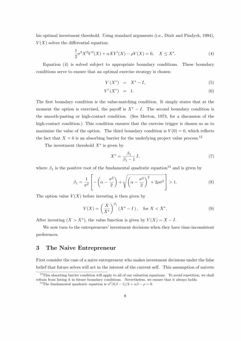
his optimal investment threshold. Using standard arguments (i.e., Dixit and Pindyck, 1994),
V (X) solves the differential equation:
12σ2X2V ′′(X) + αXV ′(X)− ρV (X) = 0, X ≤ X∗. (4)
Equation (4) is solved subject to appropriate boundary conditions. These boundary
conditions serve to ensure that an optimal exercise strategy is chosen:
V (X∗) = X∗ − I, (5)
V ′ (X∗) = 1. (6)
The first boundary condition is the value-matching condition. It simply states that at the
moment the option is exercised, the payoff is X∗ − I. The second boundary condition is
the smooth-pasting or high-contact condition. (See Merton, 1973, for a discussion of the
high-contact condition.) This condition ensures that the exercise trigger is chosen so as to
maximize the value of the option. The third boundary condition is V (0) = 0, which reflects
the fact that X = 0 is an absorbing barrier for the underlying project value process.12
The investment threshold X∗ is given by
X∗ =β1
β1 − 1I, (7)
where β1 is the positive root of the fundamental quadratic equation13 and is given by
β1 =1σ2
−
(α− σ2
2
)+
√(α− σ2
2
)2
+ 2ρσ2
> 1. (8)
The option value V (X) before investing is then given by
V (X) =(
X
X∗
)β1
(X∗ − I ) , for X < X∗. (9)
After investing (X > X∗), the value function is given by V (X) = X − I.
We now turn to the entrepreneurs’ investment decisions when they have time-inconsistent
preferences.
3 The Naive Entrepreneur
First consider the case of a naive entrepreneur who makes investment decisions under the false
belief that future selves will act in the interest of the current self. This assumption of naivete12This absorbing barrier condition will apply to all of our valuation equations. To avoid repetition, we shall
refrain from listing it in future boundary conditions. Nevertheless, we ensure that it always holds.13The fundamental quadratic equation is σ2β(β − 1)/2 + αβ − ρ = 0.
8
was first proposed by Strotz (1956), and has been analyzed in Akerlof (1991) and O’Donoghue
and Rabin (1999a, 1999b), among others. Naivete is consistent with empirical evidence
on 401(k) investment (Madrian and Shea, 2001), task completion (Ariely and Wertenbroch
(2002)) and health club attendance (DellaVigna and Malmendier (2003)).
The current self, self 0, has preferences D0(t, s), as specified in (2). Specifically, the
current self discounts payoffs during his lifetime with the discount function e−ρt for t < t1,
and discounts payoffs received by future selves with the discount function δe−ρt, for t ≥ t1.
Given the time-inconsistent preferences, future self 1 will have the discount function D1(t, s),
future self 2 will have the discount function D2(t, s), and so on. Since the naive entrepreneur
(mistakenly) believes that all future selves will act as if their discount function remains
unchanged at D0(t, s), we may effectively view the naive entrepreneur as acting as if he can
commit his future selves to behave according to his current preferences. Of course, in our
model there is no actual commitment mechanism and thus the naive entrepreneur’s optimistic
beliefs will prove incorrect.
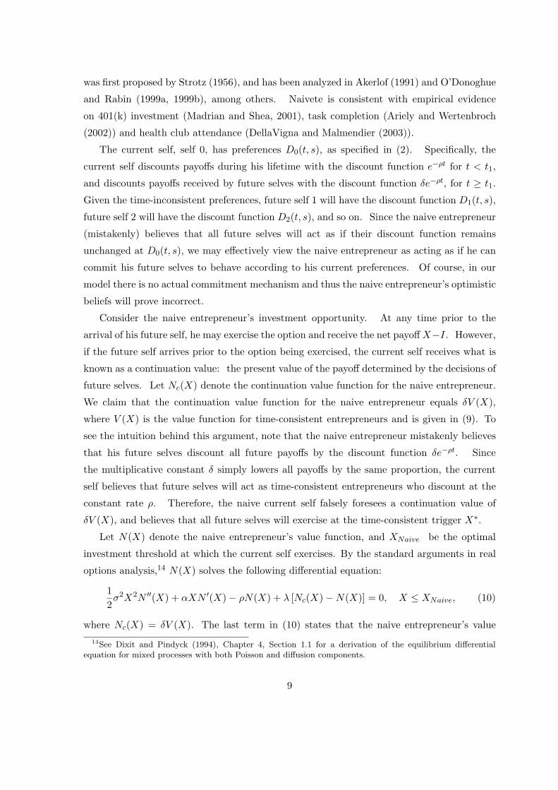
Consider the naive entrepreneur’s investment opportunity. At any time prior to the
arrival of his future self, he may exercise the option and receive the net payoff X−I. However,
if the future self arrives prior to the option being exercised, the current self receives what is
known as a continuation value: the present value of the payoff determined by the decisions of
future selves. Let Nc(X) denote the continuation value function for the naive entrepreneur.
We claim that the continuation value function for the naive entrepreneur equals δV (X),
where V (X) is the value function for time-consistent entrepreneurs and is given in (9). To
see the intuition behind this argument, note that the naive entrepreneur mistakenly believes
that his future selves discount all future payoffs by the discount function δe−ρt. Since
the multiplicative constant δ simply lowers all payoffs by the same proportion, the current
self believes that future selves will act as time-consistent entrepreneurs who discount at the
constant rate ρ. Therefore, the naive current self falsely foresees a continuation value of
δV (X), and believes that all future selves will exercise at the time-consistent trigger X∗.
Let N(X) denote the naive entrepreneur’s value function, and XNaive be the optimal
investment threshold at which the current self exercises. By the standard arguments in real
options analysis,14 N(X) solves the following differential equation:
12σ2X2N ′′(X) + αXN ′(X)− ρN(X) + λ [Nc(X)−N(X)] = 0, X ≤ XNaive, (10)
where Nc(X) = δV (X). The last term in (10) states that the naive entrepreneur’s value14See Dixit and Pindyck (1994), Chapter 4, Section 1.1 for a derivation of the equilibrium differential
equation for mixed processes with both Poisson and diffusion components.
9
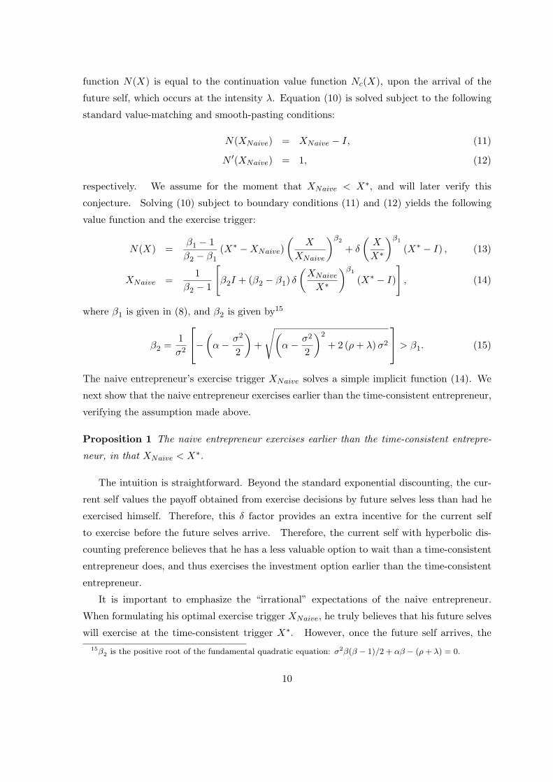
function N(X) is equal to the continuation value function Nc(X), upon the arrival of the
future self, which occurs at the intensity λ. Equation (10) is solved subject to the following
standard value-matching and smooth-pasting conditions:
N(XNaive) = XNaive − I, (11)
N ′(XNaive) = 1, (12)
respectively. We assume for the moment that XNaive < X∗, and will later verify this
conjecture. Solving (10) subject to boundary conditions (11) and (12) yields the following
value function and the exercise trigger:
N(X) =β1 − 1β2 − β1
(X∗ −XNaive)(
X
XNaive
)β2
+ δ
(X
X∗
)β1
(X∗ − I) , (13)
XNaive =1
β2 − 1
[β2I + (β2 − β1) δ
(XNaive
X∗
)β1
(X∗ − I)
], (14)
where β1 is given in (8), and β2 is given by15
β2 =1σ2
−
(α− σ2
2
)+
√(α− σ2
2
)2
+ 2 (ρ + λ) σ2
> β1. (15)
The naive entrepreneur’s exercise trigger XNaive solves a simple implicit function (14). We
next show that the naive entrepreneur exercises earlier than the time-consistent entrepreneur,
verifying the assumption made above.
Proposition 1 The naive entrepreneur exercises earlier than the time-consistent entrepre-
neur, in that XNaive < X∗.
The intuition is straightforward. Beyond the standard exponential discounting, the cur-
rent self values the payoff obtained from exercise decisions by future selves less than had he
exercised himself. Therefore, this δ factor provides an extra incentive for the current self
to exercise before the future selves arrive. Therefore, the current self with hyperbolic dis-
counting preference believes that he has a less valuable option to wait than a time-consistent
entrepreneur does, and thus exercises the investment option earlier than the time-consistent
entrepreneur.
It is important to emphasize the “irrational” expectations of the naive entrepreneur.
When formulating his optimal exercise trigger XNaive, he truly believes that his future selves
will exercise at the time-consistent trigger X∗. However, once the future self arrives, the15β2 is the positive root of the fundamental quadratic equation: σ2β(β − 1)/2 + αβ − (ρ + λ) = 0.
10
future self becomes a current self and also mistakenly believes that its future selves will
exercise at X∗.
We now turn to the case of the sophisticated entrepreneur, who correctly realizes that his
preferences are time-inconsistent and also knows that he cannot commit to a pre-determined
investment timing strategy.
4 The Sophisticated Entrepreneur
Unlike the naive entrepreneur, the sophisticated entrepreneur correctly foresees that his future
selves will act according to their own preferences. That is, self n makes his decision based
on self n’s preferences, fully anticipating that all future selves will do likewise. This leads
to time-inconsistency in the policy rule. That is, self n and self (n + 1) do not agree on the
optimal investment timing strategy.
As we will see, the solution for the sophisticated entrepreneur is non-trivial. For illustra-
tive purposes, we will begin this section with the simple case of a sophisticated entrepreneur
with just three selves: the current self will live for two more periods. We then move on
to the more complicated case of the entrepreneur with any finite number of selves N . This
is analogous to the general case of an entrepreneur with a finite lifespan. Finally, we con-
sider the more analytically tractable case in which the entrepreneur has an infinite number
of future selves.
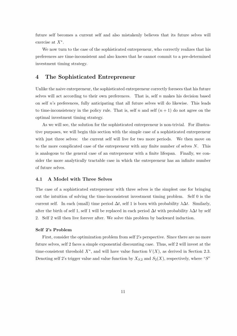
4.1 A Model with Three Selves
The case of a sophisticated entrepreneur with three selves is the simplest one for bringing
out the intuition of solving the time-inconsistent investment timing problem. Self 0 is the
current self. In each (small) time period ∆t, self 1 is born with probability λ∆t. Similarly,
after the birth of self 1, self 1 will be replaced in each period ∆t with probability λ∆t by self
2. Self 2 will then live forever after. We solve this problem by backward induction.
Self 2’s Problem
First, consider the optimization problem from self 2’s perspective. Since there are no more
future selves, self 2 faces a simple exponential discounting case. Thus, self 2 will invest at the
time-consistent threshold X∗, and will have value function V (X), as derived in Section 2.3.
Denoting self 2’s trigger value and value function by XS,2 and S2(X), respectively, where “S”
11
signifies “sophisticated,” we thus have:
S2(X) = V (X) =(
X
X∗
)β1
(X∗ − I ) , X ≤ X∗, (16)
XS,2 = X∗ =β1
β1 − 1I. (17)
Self 1’s Problem
Self 1 formulates his optimal exercise trigger XS,1, taking into account that his future self
will exercise at the trigger XS,2 = X∗, if his future self has the opportunity to exercise the
option. However, because of self 1’s hyperbolic time preferences, he values the payoff obtained
from the exercise decision by self 2 at only δ of its future value. Self 1’s problem is thus
mathematically identical to that of the naive entrepreneur, solved in Section 3. However, note
that while the naive entrepreneur in Section 3 has false beliefs, the self 1 of the sophisticated
entrepreneur has rational beliefs.
Using the result in Section 3, we may write self 1’s option value S1(X) as follows:
S1(X) = N(X) =β1 − 1β2 − β1
(X∗ −XS,1)(
X
XS,1
)β2
+ δ
(X
X∗
)β1
(X∗ − I) , (18)
for X ≤ XS,1 and where the optimal trigger strategy solves the implicit function given by
XS,1 = XNaive =1
β2 − 1
[β2I + (β2 − β1) δ
(XS,1
X∗
)β1
(X∗ − I)
]. (19)
Note that XS,1 < XS,2, as demonstrated in Proposition 1.
Self 0’s Problem
Now, we turn to the optimization problem for self 0. Self 0 will choose his optimal
exercise trigger XS,0, knowing that selves 1 and 2 will exercise at the triggers, XS,1 and XS,2,
respectively. Due to self 0’s hyperbolic preferences, in addition to discounting future cash
flows at the rate ρ, he will further discount cash flows obtained from exercise decisions by
either selves 1 or 2 by the additional factor δ.
Let Sc1(X) denote the continuation value function for self 0, self 0’s valuation of the
proceeds of exercise occurring after the arrival of self 1. The continuation value function
Sc1(X) has a recursive formulation. If self 1 is alive when his trigger XS,1 is reached, then the
option is exercised, and its payoff to self 0 is δ (XS,1 − I). If instead self 2 arrives before XS,1
is reached, then self 0’s continuation value evolves into self 1’s continuation value, Sc2(X),
where Sc2(X) = δV (X). Thus Sc
1(X) solves the following differential equation:
12σ2X2Sc′′
1 (X) + αXSc′1 (X)− ρSc
1(X) + λ [δV (X)− Sc1(X)] = 0, X ≤ XS,1, (20)
12
where the value-matching condition is given by
Sc1(XS,1) = δ (XS,1 − I) . (21)
Note that we only have the value-matching, not the smooth-pasting condition for the contin-
uation value function Sc1(X). This is intuitive since solving the continuation value function
Sc1(X) does not involve an optimality decision. The value-matching condition simply follows
from the continuity of the continuation value function. Solving (20) and (21) jointly gives
Sc1(X) = δ (X∗ − I)
(X
X∗
)β1
+ δ
[XS,1 − I −
(XS,1
X∗
)β1
(X∗ − I)
](X
XS,1
)β2
, (22)
for X ≤ XS,1.
Self 0 maximizes his value function S0(X), by taking his continuation value function
Sc1(X) computed in (22) as given and choosing his investment threshold value XS,0. Using
the standard principle of optimality, we have the following differential equation for self 0’s
value function:
12σ2X2S′′0 (X) + αXS′0(X)− ρS0(X) + λ [Sc
1(X)− S0(X)] = 0, X ≤ XS,0. (23)
Because Sc1(X) in (22) contains the Xβ2 term, the general solution to the differential
equation (23) is more complicated than the standard real options solution. In the appendix,
we show that the general solution to (23) takes the following form:
S0(X) = δ (X∗ − I)(
X
X∗
)β1
+ G0,1Xβ2 log X + AXβ2 , (24)
where
G0,1 = − λ
α + (2β2 − 1)σ2/2δ
[XS,1 − I −
(XS,1
X∗
)β1
(X∗ − I)
](1
XS,1
)β2
, (25)
While the general solution uniquely determines G0,1, it does not pin down he coefficient A
nor the investment trigger XS,0.
The constant A and the optimal trigger XS,0 are determined by appending the following
value-matching and smooth-pasting conditions:
S0(XS,0) = XS,0 − I, (26)
S′0(XS,0) = 1. (27)
Self 0’s exercise trigger XS,0 is the solution to the implicit equation
XS,0 =β2
β2 − 1I +
(β2 − β1
β2 − 1
)δ
(XS,0
X∗
)β1
(X∗ − I)− G0,1
β2 − 1X
β2S,0, (28)
13
and A = G0,0, where G0,0 is given by
G0,0 = X−β2S,0
[XS,0 − I − δ (X∗ − I)
(XS,0
X∗
)β1
−G0,1Xβ2S,0 log (XS,0)
]. (29)
We will show later that each self will exercise at a lower trigger than its future selves, in
that XS,0 < XS,1 < XS,2. The intuition is clear by using the backward induction argument.
First, self 2 will live forever, so he has time-consistent preferences and will exercise at the
time-consistent trigger X∗. Self 1, however, faces a different option exercise problem. He
knows that if self 2 arrives before he exercises, he will ultimately receive only the fraction δ of
the payoff from self 2’s exercise decision. Thus, self 1 has a less valuable option to wait than
self 2, since the longer he waits, the greater the chance that self 2 will arrive and provide a
lowered payoff. Thus, self 1 exercises earlier than self 2. Finally, the same argument holds
for self 0. If self 1 arrives before self 0 exercises, he will receive only the fraction δ of the
payoff value from self 1’s investment decision. Thus, self 0 has a lower option value to wait
than self 1, and hence exercises at a trigger lower than does self 1.
4.2 The Sophisticated Entrepreneur with Any Finite Number of Selves
In this subsection, we consider the general case of a sophisticated entrepreneur with any finite
number of selves. Self 0 is followed by self 1, who is followed by self 2, all the way through
self N . Just as in the case of three selves, one can solve the model by backward induction.
Given self (n + 1) through self N ’s exercise triggers, self n can formulate his optimal exercise
strategy, discounting any future self’s exercise proceeds by the additional factor δ. Let
Sn+1(X) be the value function for self (n + 1) and Scn+1(X) denote the continuation value
function for self n, consistent with the notations used in analysis for the three-self case.
We will only present an outline of the derivation. A full derivation of the results appears
in the appendix. Importantly, we will derive a recursive formula for the value function of
each self along with their optimal exercise triggers. This will also pave the way for the more
analytically tractable case with an infinite number of selves.
First consider self N ’s problem. Since self N is the final self, he faces the standard time-
consistent option exercise problem. Therefore, self N ’s value function SN (X) is equal to
the time-consistent entrepreneur’s value function V (X) and self N ’s exercise trigger XS,N
is also equal to the time-consistent entrepreneur’s exercise trigger X∗. The solution for the
penultimate self, self (N − 1), is also easily obtained. As discussed in the previous subsection,
the penultimate sophisticated entrepreneur faces mathematically the same problem as the
naive entrepreneur. Thus, the value function SN−1(X) for self (N − 1), the continuation value
14
function ScN (X) for self (N − 1), and the exercise trigger XS,N−1 chosen by self (N − 1) are
given by SN−1(X) = N(X), ScN (X) = δV (X), and XS,N−1 = XNaive, respectively, where
these formulas for the naive entrepreneurs are derived in Section 3.
For n ≤ N − 2, self n’s value function and exercise strategy may also be solved by
backward induction. Similar to the three-self case analysis, the continuation value function
Scn+1(X), which is self n’s valuation of the payoffs from exercise occurring after the arrival of
self (n + 1), satisfies the following differential equation:
12σ2X2Sc′′
n+1(X)+αXSc′n+1(X)−ρSc
n+1(X)+λ[Sc
n+2(X)− Scn+1(X)
]= 0, X ≤ XS,n+1, (30)
where the value-matching condition is given by
Scn+1(XS,n+1) = δ (XS,n+1 − I) . (31)
As in the three-self case, only the value-matching condition, not the smooth-pasting condition,
applies to the continuation value function Scn+1(X). The recursive relationship starts with
the known solutions XS,N−1 = XNaive and ScN (X) = δV (X). The solutions for Sc
n+1(X) for
n = 0, · · · , N − 2 are presented in the appendix. We take the trigger XS,n+1 as given, when
we calculate the continuation value function Scn+1(X). We solve for XS,n+1 as part of the
optimization problem for self (n + 1). This is to which we now turn.
The sophisticated entrepreneur’s value function Sn+1(X) solves the differential equation:
12σ2X2S′′n+1(X)+αXS′n+1(X)−ρSn+1(X)+λ
[Sc
n+2(X)− Sn+1(X)]
= 0, X ≤ XS,n+1, (32)
where the value-matching and smooth-pasting conditions are given by
Sn+1(XS,n+1) = XS,n+1 − I, (33)
S′n+1(XS,n+1) = 1. (34)
The solutions for the value functions Sn+1(X) are presented in the appendix. Most impor-
tantly, however, are the optimal exercise triggers chosen by each of the selves. The optimal
exercise trigger for self n, satisfies the implicit function:
XS,n+1 =β2
β2 − 1I+
(β2 − β1
β2 − 1
)δ
(XS,n+1
X∗
)β1
(X∗ − I)− 1β2 − 1
N−2−n∑
k=1
kGn+1,k Xβ2S,n+1 (log XS,n+1)
k−1 ,
(35)
for n + 1 ≤ N − 2, and where the triggers XS,N and XS,N−1 are equal to X∗ and XNaive,
respectively. The constants Gn+1,k = Cn+1,k are given in (B.5), for 1 ≤ k ≤ N − 2− n.
The following proposition demonstrates that each self’s trigger value is lower than that
of its future self. That is, XS,0 < XS,1 < ... < XS,N . This makes intuitive sense since
15

the time-inconsistency problem will be greater for the earlier selves, as earlier selves have a
greater number of future selves whose decisions may detrimentally influence earlier selves’
value functions.
Proposition 2 XS ,n is increasing in n.
For the case of a finite number of selves, we can now easily prove that the sophisticated
entrepreneur will exercise earlier than the naive entrepreneur, who in turn will invest earlier
than the time-consistent entrepreneur. This is summarized in the following proposition.
Proposition 3 For the sophisticated entrepreneur with a finite number of selves N , XS,0 <
XNaive < X∗.
For the sophisticated entrepreneur, each additional future self introduces an extra layer
of potentially detrimental exercise behavior from the standpoint of the current self’s utility,
magnifying the problem of time-inconsistency. In an effort to avoid the detrimental effect of
future selves’ exercise decisions, the current self finds it optimal to exercise earlier than he
otherwise would, in order to lessen the chance of failing to exercise prior to the arrival of his
future selves. This will be discussed in greater detail in Section 4.4.
4.3 The Sophisticated Entrepreneur with an Infinite Number of Selves
We have so far fixed the number of selves to a finite number. Although we have delivered the
intuition on the effect of hyperbolic discounting on investment decision via the finite N -self
model, the model solution may be substantially simplified by proceeding to the case with a
countably infinite number of selves. For a fixed number of selves N , we have shown that
(i) self N chooses the time-consistent investment trigger X∗ and (ii) the investment trigger
for self n is lower than the investment trigger for self (n + 1). Given the monotonicity of the
investment trigger and the fact that all investment triggers are positive, we may conjecture
that the investment trigger for self 0 converges to the steady-state limiting investment trigger,
when the total number of selves N goes to infinity.
When we have infinite number of selves, the sophisticated entrepreneur faces the same
time-invariant option exercising problem, for any self n. That is, the sophisticated entre-
preneur’s optimization problem does not depend on n. The stationary solution will involve
searching for a fixed-point to the investment exercise problem.16 Specifically, suppose that16We here exclusively focus on the most natural Markov perfect equilibrium, in which all selves exercise at
the same trigger. However, it is conceivable that other equilibria may exist.
16
all stationary future selves exercise at the trigger XS . Then, XS will represent the (intra-
personal) equilibrium investment trigger if the current self’s optimal exercise trigger, condi-
tional on the fact that future selves will exercise at XS , is also XS .
Before solving for the intra-personal equilibrium exercise trigger, we consider the current
self’s exercise strategy conditional on an assumed future self exercise trigger. Let X denote
the conjectured exercise trigger by the future selves. Let Φ(X) denote the entrepreneur’s
optimal exercise trigger, as a function of X, the conjectured exercise trigger chosen by his
future selves.
We solve the entrepreneur’s investment trigger by working backwards. Let S(X; X) and
Sc(X; X) denote the entrepreneur’s value function and the continuation value function, re-
spectively, conditioning on the conjectured exercise trigger X chosen by his future selves.
As in the previous analysis, first consider the entrepreneur’s continuation value function
Sc(X; X). Since all future selves are conjectured to exercise at the same trigger, X, the
continuation value function is therefore given by δ times the present value of receiving the
payoff value X − I, when the entrepreneur exercises at the trigger X. Using the standard
present value analysis with stopping time (Dixit and Pindyck (1994)), we thus have
Sc(X; X) =
δ(
XX
)β1(X − I
), for X < X,
δ (X − I) , for X ≥ X.
(36)
Having derived the continuation value function Sc(X; X), we now turn to the sophisticated
entrepreneur’s investment optimization problem. Using the standard argument, we have
12σ2X2 ∂2S(X; X)
∂X2+ αX
∂S(X; X)∂X
− ρS(X; X) + λ[Sc(X; X)− S(X; X)
]= 0, (37)
for X ≤ X. The differential equation (37) is solved subject to the following value-matching
and smooth-pasting conditions
S(Φ(X); X
)= Φ(X)− I, (38)
∂S(Φ(X); X
)
∂X= 1. (39)
We may obtain the intra-personal equilibrium sophisticated exercise trigger, XS , by sub-
stituting the continuation value function Sc(X; X) given in (36) into the differential equation
(37), applying boundary conditions (38) and (39), and solving for the value function S(X; X)
and the exercise trigger Φ(X). We may then impose the intra-personal equilibrium condi-
tion that all selves exercise at the same trigger: Φ(XS) = XS . Define the intra-personal
17

equilibrium value function S(X; XS) ≡ S(X), we thus obtain the solution of the stationary
sophisticated entrepreneur problem:
S(X) =
[δ
(X
XS
)β1
+ (1− δ)(
X
XS
)β2
](XS − I) , (40)
XS =β
β − 1I, (41)
where
β = β1δ + β2(1− δ). (42)
Note that the value of the sophisticated entrepreneur’s option is equal to a weighted aver-
age of two time-consistent present value functions,(
XXS
)β1(XS − I) and
(XXS
)β2(XS − I),
where the weights are δ and (1− δ), respectively. Both present value functions represent
the value to a time-consistent entrepreneur of receiving the exercise payoff of (XS − I) when
the payoff value X reaches the trigger XS . However, the first present value uses the discount
rate ρ with the implied option parameter β1, and the second uses the discount rate (ρ + λ)
with the implied option parameter β2.
The sophisticated trigger XS may be obtained by using the standard real options analysis,
if we replace the standard option parameter with β, the weighted average of β1 and β2, with
δ and (1− δ) as respective weights.17 The exercise trigger XS for the sophisticated agent is
equal to the trigger for a time consistent agent, whose subjective discount rate ρ is given by
ρ = σ2β(β − 1
)/2 + αβ. Note that the entrepreneur’s investment threshold decreases with
the degree of time-inconsistency, in that ∂XS/∂δ > 0. Just as in the case with finite selves,
the sophisticated entrepreneur invests earlier than the naive entrepreneur. Proposition 4
demonstrates this timing result that is the stationary case analog to Proposition 3.
Proposition 4 The sophisticated entrepreneur in the stationary case exercises earlier than
the naive entrepreneur, who in turn exercises earlier than the time-consistent entrepreneur,
in that XS < XNaive < X∗.
4.4 Discussion
4.4.1 The Timing of Investment
Propositions 3 and 4 demonstrate that time-inconsistent entrepreneurs invest earlier than
time-consistent entrepreneurs. Moreover, the sophisticated time-inconsistent entrepreneur17When λ = ∞, we uncover the standard NPV rule (note that β2 = ∞ and XS = I). Intuitively, when the
future self arrives in no time, then the effective discount rate for the entrepreneur becomes ρ + λ = ∞. As aresult, the option value of waiting evaporates due to the sufficiently high discounting.
18
invests even earlier than the naive time-inconsistent entrepreneur. In this section we discuss
these results and their implications.
The first fundamental result is the precise trade-off between the benefits of waiting to
invest and the increased impatience driven by time-inconsistent discounting. In our in-
tertemporal stochastic setting, as is well-known from real options theory, an entrepreneur
holds a valuable option to wait. This option to wait is what drives the time-consistent
entrepreneur to exercise when the option is sufficiently in the money, as embodied by the
distance between X∗ and I. Now, when we introduce the time-varying impatience driven
by time-inconsistent preferences, we then have a force that counteracts the benefits of wait-
ing for uncertainty to resolve itself. This counteracting force is caused by the current self’s
motivation to exercise before the future selves take control of the exercise decision, because
the payoff to the current self from future exercise is discounted by the factor δ in addition
to the conventional exponential discounting. Therefore, the lowered value of the option to
wait induces time-inconsistent entrepreneurs to exercise earlier than the time-consistent en-
trepreneur. Time-inconsistency reduces, but does not eliminate, the option value of waiting
(I < XS < XNaive < X∗).
The second fundamental result is the distinction between sophisticated and naive entre-
preneurs. Sophisticated entrepreneurs invest even earlier than naive entrepreneurs. The
intuition is relatively simple. While naive entrepreneurs are optimistic in that they in-
correctly forecast that their future selves will behave according to their current preferences,
sophisticated entrepreneurs correctly forecast that their future selves will invest suboptimally
relative to their current preferences. The realistic pessimism of sophisticated entrepreneurs
compels them to invest earlier than naive entrepreneurs, so as to lessen the probability that
future selves will take over the investment decision and invest suboptimally. This result is
referred to by O’Donoghue and Rabin (1999a) as the “sophistication effect.” The fact that
sophisticated entrepreneurs are concerned about the suboptimal timing decisions of future
selves further erodes the value of their option to wait relative to that of naive entrepreneurs.
Figure 1 plots the option values for the time-consistent entrepreneur, the naive entrepre-
neur, the sophisticated entrepreneur with an infinite number of selves, and the sophisticated
entrepreneur a finite number of selves (N = 5). For each type of entrepreneur, the option
value smoothly pastes to the project’s net payoff value, (X − I), at the entrepreneur’s exer-
cise trigger. For each value of X prior to exercise, the vertical distance between the option
value and the payoff value measures the value of the option to wait. Note that at all levels
of X prior to exercise, the time-consistent entrepreneur has the most valuable option to wait,
followed by the naive entrepreneur, then the sophisticated entrepreneur with a finite number
19
of selves, and finally the sophisticated entrepreneur with an infinite number of selves.
[Insert Figure 1 here.]
4.4.2 Comparison with Models of Competition
Several authors have expanded the real options framework to include strategic competition.18
In such models, competitive pressure from the exercise decisions of other investors motivates
early exercise so as to avoid the costs of preemption. Thus, in terms of empirical implications,
both the competitive models and our model of time-inconsistent preferences make similar
predictions. To distinguish between these two theoretical explanations for markets that
display early exercise of investment options, one must determine whether one finds multiple
firms competing over similar investment opportunities, or small numbers of time-inconsistent
entrepreneurs with unique investment opportunities.
This analogy between inter-firm competition and time-inconsistency provides an inter-
esting framework for interpreting this model’s results. Essentially, rather than competing
against other entrepreneurs, the time-inconsistent entrepreneur is competing against its fu-
ture selves. With interpersonal competition, agents fear the costs of being preempted by
others. With intra-personal competition, agents fear being preempted by their future selves.
Consider the naive entrepreneur. He fears being preempted by his future selves simply
because he values the payoff realized from exercise decisions by his future selves less than the
payoff from his current self’s investment decision (even after taking into account the standard
exponential discounting). In our model, this effect due to fear of preemption is analogous to
the effect of competition which causes the value to be reduced by (1− δ) fraction.19 Now
consider the sophisticated entrepreneur. In addition to fearing being preempted because
of additional impatience (reflected by δ < 1), he also faces preemption costs due to the
suboptimal exercise decisions of future selves. One could view this as simply a larger cost
of preemption than that of the naive entrepreneur, or as facing repeated competition from
a sequence of future entrants. Intuitively, the naive entrepreneur is myopic and only worries
about the immediate threat of preemption, whereas the sophisticated entrepreneur is forward-
looking and concerned with all future threats of preemption.20
18See Smets (1993), Williams (1993), Grenadier (1996, 2002), and Lambrecht and Perraudin (2003).19Trigeorgis (1991) provides a model of competition driven by competitors arriving randomly according to
a jump process that is clearly in the spirit of this analogy.20In the extreme case in which δ = 0, both the naive and sophisticated entrepreneurs face the “risk of ruin”
from preemption, analogous to the bond price process with a Poisson jump described in Merton (1971). Insuch a case, both the naıve and sophisticated entrepreneurs act “as if” they are time-consistent but with adiscount rate of (ρ + λ).
20
While in reduced form, our model of time-inconsistent entrepreneurs’ investment decisions
shares some similar features with models of competition, our model is driven by a very differ-
ent economic mechanism. It is only possible to provide precise predictions on his investment
threshold by specifying the entrepreneur’s beliefs and analyzing his optimization problem. In
addition, when we later extend the model to allow for payoffs to be paid as flows over time,
we will find that time-inconsistent entrepreneurs actually invest later than time-consistent
entrepreneurs. This provides opposite implications than models of competition.
4.4.3 Implications for Real Asset Markets
In the real options literature, typical parameterizations imply that investment occurs only
when the project value is much greater than the investment cost. It is not unusual to see
such models predict that investment will only occur when the present value of the project
is double the investment cost. This has two clear empirical implications. First, there is
unlikely to be oversupply, in the sense that cautious entrepreneurs do not invest until there
is a large cushion in terms of net present value. Second, as shown in Grenadier (2002),
with such a large net present value cushion, it becomes almost impossible for there to be any
ex-post losses. Specifically, with typical parameterizations, the probability of the project’s
value five (or even ten) years after investment being below the investment cost is close to
zero. This makes the implications of standard real options models difficult to reconcile with
real world bankruptcies and foreclosures.
In the case of time-inconsistent entrepreneurs (and even more so for the specific case of
sophisticated entrepreneurs), investment may occur much earlier than in the time-consistent
case. For example, in Figure 1, the time-consistent entrepreneur exercises at a net present
value of X∗ − I = 1.88, while the sophisticated entrepreneur exercises at a net present value
of XS − I = 0.747. Thus, the time-consistent entrepreneur exercises at a net present value
that is just over 150% greater than that of the sophisticated entrepreneur. With smaller net
present value cushions, we are more likely to see periods of oversupply. Even with a moderate
time-to-build factor, projects can come online once demand has declined. Similarly, the
probabilities of ex-post losses can increase dramatically.
Consider again the real estate overbuilding example in the Introduction. Williams (2001)
states that land (both improved and unimproved) is primarily held and developed by noninsti-
tutional investors (such as individuals and private partnerships), rather than by institutional
investors (such as pension funds). These noninstitutional investors in turn sell the developed
properties to institutional investors. Such developers are termed “merchant builders.” If it
is the case that noninstitutional investors are more likely to have time-inconsistent prefer-
21
ences, then merchant builders may accept lower returns from development in order to protect
themselves against the sub-optimal development choices of their future selves. Such early
development may be a contributor to the tendency for developers to overbuild. In fact,
merchant builders are often blamed for causing overbuilding in U.S. office markets.
5 An Extension: The Flow Payoff Case
While some real world examples may fit in the lump sum payoff setting that we have analyzed,
there are other situations under which the investment payoffs are given in flows over time. For
time-consistent entrepreneurs, the lump sum and the flow payoff cases are equivalent after
adjusting for discounting. However, we show that this seemingly minor alteration generates
fundamentally different predictions about investment decisions and provide new economic
insights, when entrepreneurs have time-inconsistent preferences.
In the flow payoff case, after the entrepreneur irreversibly exercises his investment option
at some stopping time τ , he obtains a perpetual stream of flow payments {p(t) : t ≥ τ}.Here, the payoffs are assumed to be non-tradable for the same reason as for the lump sum
payoff case treated earlier. For example, the flow payoffs may be contingent on the unique
skills of the entrepreneur, or there may be moral hazard or adverse selections issues that can
undermine the selling of the cash flow stream. Assume that the flow payoff process p follow
a geometric Brownian motion process:
dp(t) = αp(t)dt + σp(t)dBt, (43)
where we assume α < ρ for convergence. The entrepreneur thus will evaluate the invest-
ment project and choose his investment time optimally based on his hyperbolic discounting
preference.
Unlike the lump sum case in which the net payoff value upon option exercise is simply given
by (X − I), the payoff value for the flow case depends on the entrepreneur’s time preferences.
Let M(p) denote the present value of the future cash flows. Using the hyperbolic discounting
function given in (2), we have
M(p) = E
[∫ T
0e−ρtp(t)dt +
∫ ∞
Tδe−ρtp(t)dt
]= γ
p
ρ− α, (44)
where
γ =ρ + δλ− α
ρ + λ− α≤ 1, (45)
and where T has an exponential distribution with mean 1/λ, and the expectation is taken
22
over the joint distribution of T and p(t).21 Therefore, the net present value of the payoff from
exercise is M(p)− I.
If the entrepreneur has time-consistent preferences (δ = 1 or λ = 0), then the present
value is given by M(p) = p/(ρ− α), the standard result. When the entrepreneur has time-
inconsistent preferences, the present value M(p) of the flow payoffs is less than that for
the time-consistent entrepreneur, in that γ < 1. A stronger degree of time-inconsistency
(manifested by a lower δ or a higher λ) implies a lower present value M(p) as seen in (44).
Unlike the lump-sum payoff case, the time-inconsistency not only lowers the option value of
waiting, but also reduces the project’s payoff value M(p) upon option exercise. Since both
the option value and the project payoff values are lowered by hyperbolic discounting, a priori,
the time-inconsistent entrepreneur may invest either earlier or later than a time-consistent
entrepreneur when his payoffs are given in flow terms.
5.1 The Time-Consistent Entrepreneur
First consider the benchmark case in which all cash flow payoffs are discounted at the constant
rate ρ. Let v(p) denote the entrepreneur’s value function and p∗ be his optimal investment
threshold to be determined. By standard arguments, the value function v(p) solves the
following differential equation:
12σ2p2v′′(p) + αpv′(p)− ρv(p) = 0, p ≤ p∗, (46)
subject to the following value-matching and smooth-pasting conditions:
v (p∗) =p∗
ρ− α− I, (47)
v′ (p∗) =1
ρ− α. (48)
21In order for the entrepreneur’s problem to make sense in the flow payoff setting, we must restrict theparameter region to ensure the existence of an intra-personal equilibrium. Specifically, we need to ensure thata trigger strategy defines the optimal stopping region. The precise condition needed is specified in AppendixB, in Chapter 4, of Dixit and Pindyck. (For the lump-sum case, this condition is always satisfied.) Thistranslates into the condition
λδβ1
�ps
ρ− α− I
�<
ρ + λδ − α
ρ− αps,
where ps is the sophisticated equilibrium trigger that appears in (63). Note that this will also ensure theexistence of a naive solution, since Proposition 6 demonstrates that the naive trigger is greater than thesophisticated trigger.
23

The value function v(p) is given by
v(p) =
(pp∗
)β1(
p∗ρ−α − I
), p < p∗,
pρ−α − I, p ≥ p∗,
(49)
and the investment exercise trigger p∗ is
p∗ =β1
β1 − 1(ρ− α) I. (50)
It is immediate to note that the investment threshold expressed in the present value term
for the flow payoff case, p∗/ (ρ− α), is equal to X∗, the investment threshold for the corre-
sponding lump sum payoff case. This equivalence no longer holds when the entrepreneur has
time-inconsistent preferences. We next analyze the time-inconsistent entrepreneur’s invest-
ment decision when the payoffs are given in flows.
5.2 The Naive Entrepreneur
Now consider the case in which the entrepreneur naively assumes that future selves will
behave according to his current preferences. Following the same procedure as in the lump
sum payoff case, we first compute the continuation value function and then solve for the value
function and the investment trigger.
As in the lump sum payoff case, the naive entrepreneur falsely believes that future selves
will exercise at the time-consistent trigger p∗. Using the same argument as the one for
the naive entrepreneur with lump sum payoffs, the naive entrepreneur’s continuation value
function nc(p) is thus given by
nc(p) =
δ(
pp∗
)β1(
p∗ρ−α − I
), if p < p∗,
δ(
pρ−α − I
), if p > p∗.
(51)
For the lump sum payoff case, time-inconsistency only lowers the option value of waiting,
not the project payoff value upon option exercise. For the flow payoff case, we have shown
that the project payoff value M(p) is also lowered by time-inconsistent preferences. It is
thus conceivable that hyperbolic discounting may have a stronger effect on the project payoff
value than on the option value of waiting. If so, the net effect of hyperbolic discounting
on investment may lead to a further delayed investment compared with the benchmark with
time-inconsistent preferences. This intuition is consistent with the results in O’Donoghue and
Rabin (1999a). They show that if the benefits are more distant, the agent may procrastinate.
24
Motivated by these considerations, we conjecture and then later verify that the investment
trigger for the naive entrepreneur is larger than the time-consistent investment trigger p∗.
Note that the continuation value function nc(p) given in (51) differs depending on whether
p is larger or smaller than p∗. Since we conjecture that the naive entrepreneur’s exercise
trigger pnaive is larger than p∗, we thus naturally need to divide the regions for p into two
and compute the corresponding value functions jointly.
Let nl(p) and nh(p) denote the naive entrepreneur’s value function n(p) for p < p∗ and
p ≥ p∗ regions, respectively. Let pnaive denote the selected exercise trigger by the naive
entrepreneur. As stated earlier, we conjecture and then verify pnaive > p∗.
First consider the higher region p ≥ p∗. Following the same argument as in the lump sum
payoff case, the value function nh(p) satisfies:
12σ2p2n′′h(p) + αpn′h(p)− ρnh(p) + λ
[δ
(p
ρ− α− I
)− nh(p)
]= 0, p ≥ p∗, (52)
where we have used the continuation value function given in (51) in the higher region. The
general solution for nh(p) is given in (A.14). This general solution is solved with the following
standard value-matching and smooth-pasting conditions:
nh(pnaive) = M(pnaive) = γpnaive
ρ− α− I, (53)
n′h(pnaive) = M ′(pnaive) =γ
ρ− α. (54)
Now consider the lower region p < p∗. Based on our conjecture pnaive > p∗, the naive
entrepreneur will not invest in the lower region. By the standard argument, the value function
nl(p) for the lower region satisfies:
12σ2p2n′′l (p) + αpn′l(p)− ρnl(p) + λ
[δ
(p
p∗
)β1(
p∗
ρ− α− I
)− nl(p)
]= 0, p < p∗, (55)
where we have used the continuation value function for the lower region given in (51). The
general solution for nl(p) is given in (A.16). Finally, we provide boundary conditions for
nl(p), which connect nl(p) with nh(p) at the boundary p∗. We require that the value function
n(p) is continuously differentiable at p∗ (see Dixit (1993), Section 3.8), in that
nl(p∗) = nh(p∗), (56)
n′l(p∗) = n′h(p∗). (57)
We also prove that the naive entrepreneur will invest later than the time-consistent en-
trepreneur, in that p∗ < pnaive. Therefore, we have verified the presumption for our solution
methodology sketched out here.
25
Proposition 5 For the flow payoff case, the naive entrepreneur invests later than the time-
consistent entrepreneur, in that p∗ < pnaive.
5.3 The Sophisticated Entrepreneur
Now, consider the flow payoff case for the sophisticated entrepreneur. For analytical tractabil-
ity, we analyze the case with an infinite number of selves. However, nothing substantive would
change if we instead modeled the case with a finite number of selves, as we have done earlier
for the case with lump sum payoffs.
The intra-personal equilibrium trigger for sophisticated entrepreneurs with flow payoffs
represents the solution to a fixed-point problem. In a stationary intra-personal equilibrium,
the current self’s optimal exercise trigger, conditional on an assumed trigger for future selves,
must be the same as that of future selves. Let p denote the current self’s conjectured trigger
chosen by future selves. Let s(p; p) and sc(p; p) denote the value function and the continuation
value function, respectively, conditioning on the conjectured trigger p of future selves.
We first calculate the continuation value function sc(p; p). Since all future selves exercise
at the same trigger p in the stationary setting, using the present value argument, we may
compute the continuation value sc(p; p) as follows:
sc(p; p) =
δ(
pp
)β1(
pρ−α − I
), for p < p,
δ(
pρ−α − I
), for p ≥ p.
(58)
Let ϕ(p) denote the sophisticated entrepreneur’s optimal exercise trigger, expressed as a
function of the current self’s conjectured investment trigger p by future selves. Using the
continuation value function sc(p), we may write the sophisticated entrepreneur’s value func-
tion as follows:
12σ2p2 ∂2s(p; p)
∂p2+ αp
∂s(p; p)∂p
− ρs(p; p) + λ [sc(p; p)− s(p; p)] = 0, p ≤ p, (59)
where the value-matching and smooth-pasting conditions are given by
s (ϕ (p) ; p) = M (ϕ (p)) = γϕ(p)ρ− α
− I, (60)
∂s (ϕ (p) ; p)∂p
= M ′ (ϕ (p)) =γ
ρ− α. (61)
Let ps denote the intra-personal equilibrium sophisticated exercise trigger. The equi-
librium condition requires that all selves of the entrepreneur exercise at the same trigger,
in that ϕ (ps) = ps. Let s(p) denote the intra-personal equilibrium value function, in that
26

s(p; ps) ≡ s(p). Solving the differential equation (59) subject to the boundary conditions
(60)-(61) and imposing the equilibrium conditions gives the following equilibrium value func-
tion s(p) and the equilibrium exercise trigger ps for the sophisticated entrepreneur:
s(p) = δ
(p
ps
)β1(
ps
ρ− α− I
)+
[γ
ps
ρ− α− I − δ
(ps
ρ− α− I
)](p
ps
)β2
, (62)
ps = (ρ− α)β1δ + β2 (1− δ)
(β2 − 1) γ − (β2 − β1) δI. (63)
Having analyzed the exercise triggers for the time-consistent, naive and sophisticated
entrepreneurs, we now may state the following proposition.
Proposition 6 For the case with flow payoffs, the naive entrepreneur exercises later than
the sophisticated entrepreneur, who exercises later than the time-consistent entrepreneur, in
that pnaive > ps > p∗.
5.4 Discussion
As demonstrated by Propositions 5 and 6, the flow payoff case provides very different results
from the lump sum payoff case. This result is due to the interaction of two conflicting
forces for the flow payoff case. First, as we know from the case with lump-sum payoffs,
hyperbolic discounting increases the desire to exercise earlier, as this allows the entrepreneur
to protect himself from the “sub-optimal” investment decision of future selves. Second, for
the case with flow payoffs, the hyperbolic entrepreneur actually receives a “lower” present
value M(p) for the flow payoffs than would a time-consistent agent. This is apparent from the
γ parameter that enters the payoff value M(p). This lowered payoff from the current self’s
exercise motivates the hyperbolic entrepreneur to wait longer before exercising, to justify the
investment cost I. We show that the second effect dominates the first effect.22
Figure 2 plots the option values for the time-consistent, naive and sophisticated entre-
preneurs. Also plotted is the net present values (upon immediate exercise) for the time-
consistent entrepreneur, p/(ρ−α)−I, and for the time-inconsistent entrepreneurs, M(p)−I.
For each value of p prior to exercise, the vertical distance between the option value and the
payoff value measures the value of the option to wait. Because the time-inconsistent en-
trepreneur values the project payoff less than the time-consistent entrepreneur (γ < 1), the22If instead of using an infinite horizon for the cash flows we moved to a finite horizon T , then we would find
for a particular finite horizon the two effects would exactly offset each other. That is, there exists a T ∗ in theflow payment case such that for T = T ∗ the sophisticated and time-consistent entrepreneurs would exerciseat the same time. For T < T ∗ the sophisticated entrepreneur would exercise earlier than the time-consistententrepreneur, and for T ≥ T ∗ the sophisticated entrepreneur would exercise later than the time-consistententrepreneur.
27
time-inconsistent entrepreneur naturally has weaker incentives to exercise the investment op-
tion than the time-consistent entrepreneur. Thus, the time-inconsistent entrepreneur invests
later than the time-consistent entrepreneur, whether naive or sophisticated. Now we turn to
the comparison between the sophisticated and naive entrepreneurs.
As in the lump sum payoff case, the sophisticated entrepreneur invests earlier than the
naive entrepreneur. The sophisticated entrepreneur has a greater desire to invest earlier
than the naive entrepreneur so as to protect himself against the behavior of future selves
due to his belief that his future selves will not behave in his own interest. Therefore, the
option value to wait for the sophisticated entrepreneur is lower because its future selves will
exercise at suboptimal exercise triggers (from the vantage of the current self). Figure 2
confirms our intuition. While the payoff upon option exercise is the same for both the naive
and the sophisticated entrepreneurs, the naive entrepreneur’s value function n(p) is always
greater than s(p). Therefore, the threshold at which the option value and the straight line
are connected and smoothly pasted must be higher for the naive entrepreneur than for the
sophisticated entrepreneur. Note that our argument holds for both the lump sum and flow
payoff cases. Hence, we may conclude that the sophisticated entrepreneur always invests
earlier than the naive entrepreneur does, regardless of whether the payoffs are lump sum or
flows. This result is referred to by O’Donoghue and Rabin (1999a) as the “sophistication
effect” and holds true under both the lump sum and flow payoff settings.
[Insert Figure 2 here.]
6 The Interaction of Time-Inconsistent Entrepreneurs: TheCase of Competitive Industry Equilibrium
In this section we model the perfectly competitive equilibrium outcome when the industry is
comprised of sophisticated hyperbolic entrepreneurs. It is an equilibrium extension of the
flow payoff case of Section 5, where the entrepreneurs acted as monopolists. The competitive
equilibrium framework that we use is similar to that of Leahy (1993) and Dixit and Pindyck
(1994). The key contribution of this section is the extension of the equilibrium to the case
with time-inconsistent entrepreneurs.
Consider an industry comprised of a large number of entrepreneurs. Each entrepreneur
has the option to irreversibly undertake a single investment by paying an up-front investment
cost of I at chosen time τ . Investment is irreversible, in that exit from the industry is
not permitted. Upon investment, the project yields a stream of stochastic (profit) flow of
28
{p(s) : s ≥ τ} forever.23 The industry is perfectly competitive, in that each unit of output
is small in comparison with industry supply, Q(t). Thus, each entrepreneur acts as a price
taker. The equilibrium price is determined by the condition equating industry supply and
demand. Each entrepreneur takes as given the stochastic process of price p. In the rational
expectations equilibrium, this conjectured price process will indeed be the market clearing
price.
The price of a unit of output is given by the industry’s inverse demand curve
p(t) = θ(t) ·D (Q(t)) , (64)
where D′(Q) < 0 and θ(t) is a multiplicative shock and is given by following the geometric
Brownian motion process:
dθ(t) = αθ(t)dt + σθ(t)dBt. (65)
Over an interval of time in which no entry takes place, Q( · ) is fixed, and thus the price
process p evolves as follows:
dp(t) = αp(t)dt + σp(t)dBt. (66)
Given the multiplicative shock specification of the demand curve in (64), entry by new entre-
preneurs causes the price process to have an upper reflecting barrier. Thus, in this simple
setting, each price taking entrepreneur will take the process (66) with an upper reflecting
barrier as given. In the rational expectations equilibrium, the entry response by entrepre-
neurs who assume such a process will lead precisely to the supply process that equates supply
and demand.24
6.1 Equilibrium with Time-Consistent Entrepreneurs
As a benchmark, consider an industry comprised of time-consistent entrepreneurs. Conjecture
that the equilibrium entry will be at the trigger p∗eq, and thus in equilibrium the price process
will have an upper reflecting barrier at p∗eq. Consider the value of an active entrepreneur, one
that has already paid the entry cost and is producing output. Let G(p) denote the value of23We assume no variable costs of production, and thus the process p represents cash flow process, as in
Section 5.24While we solve for the equilibrium comprised of sophisticated entrepreneurs, we do not construct an
equilibrium for the case of naive entrepreneurs. This is due to the problematic nature of defining an equilibriumfor naive entrepreneurs. While the literature on naive hyperbolic preferences provides a well-defined notionof a current self’s expectations regarding future selves’ behavior, there is no standard assumption regardingwhat naive entrepreneurs forecast for others’ current and future selves. For example, do naive entrepreneursbelieve that other entrepreneurs possess self control, or do they believe that only they themselves possess selfcontrol? The implications for either assumption make for a very complex equilibrium.
29
an active entrepreneur. By the standard argument, G(p) satisfies the equilibrium differential
equation:12σ2p2G′′(p) + αpG′(p)− ρG(p) + p = 0, p ≤ p∗eq. (67)
The impact of the reflecting barrier necessitates the boundary condition25:
G′(p∗eq) = 0. (68)
Similarly, let F (p) denote the value of an inactive entrepreneur, its value prior to investing.
By the standard argument, F (p) satisfies the following differential equation:
12σ2p2F ′′(p) + αpF ′(p)− ρF (p) = 0, p ≤ p∗eq. (69)
The inactive entrepreneur’s investment trigger is determined by value-matching and smooth-
pasting conditions. In equilibrium, the entry trigger must equal the conjectured reflecting
barrier p∗eq, in that
F(p∗eq
)= G(p∗eq)− I, (70)
F ′ (p∗eq)
= G′(p∗eq). (71)
The solution to this equilibrium system is:
F (p) = 0, (72)
G(p) = − I
β1 − 1
(p
p∗eq
)β1
+p
ρ− α, p ≤ p∗eq, (73)
p∗eq = p∗ =β1
β1 − 1(ρ− α) I, (74)
with a price process governed by a geometric Brownian motion process (66) with a reflecting
barrier at p∗.
The equilibrium is clearly very intuitive. Free entry ensures that the value of an inactive
entrepreneur is zero. The value of an active entrepreneur is equal to the present value of
future cash flows, where the reflecting barrier ensures that the value of an active entrepreneur
at entry is equal to the cost of entry, G(p∗eq) = I. Finally, as has been demonstrated by
Leahy (1993) and others, the exercise trigger for a perfectly competitive industry equals the
monopolist trigger p∗. The intuition is that the reflecting barrier has two exactly opposing
effects: it lowers the value of the payoff from exercise (since the future cash flow is capped
at the barrier), while it also lowers the option value of waiting.25See Malliaris and Brock (1982, p. 200).
30
6.2 Equilibrium with Sophisticated Entrepreneurs
We now consider the equilibrium for an industry, which is comprised of time-inconsistent
entrepreneurs with sophisticated beliefs. All entrepreneurs are symmetric with respect to
sharing the same values of λ and δ. Conjecture that the equilibrium entry will occur at the
trigger peq, and thus in equilibrium the price process will have an upper reflecting barrier at
peq. Consider the value of an active entrepreneur, one that has already paid the entry cost
and is producing output. Let g(p) and gc(p) denote the value function and the continuation
value function of an active entrepreneur, respectively.
First consider the solution for the continuation value function, gc(p). Following the same
argument used earlier, gc(p) satisfies the following differential equation:
12σ2p2g′′c (p) + αpg′c(p)− ρgc(p) + δp = 0, p ≤ peq, (75)
subject to the boundary condition at the upper reflecting barrier peq:
g′c(peq) = 0. (76)
Solving (75) subject to (76) gives the solution for the continuation value:
gc(p) = − δ
ρ− α
peq
β1
(p
peq
)β1
+δp
ρ− α, p ≤ peq. (77)
Now we turn to the solution of the value function g(p) for an active entrepreneur. By the
standard argument, g(p) satisfies the following differential equation:
12σ2p2g′′(p) + αpg′(p)− ρg(p) + p + λ[gc(p)− g(p)] = 0, p ≤ peq, (78)
where gc(p) is the continuation value given in (77). The impact of the reflecting barrier
necessitates the boundary condition:
g′(peq) = 0. (79)
Just as in the case of the previously derived equilibrium with time-consistent entrepreneurs,
free-entry will ensure that the value of an active entrepreneur will equal the cost of investment
at the entry trigger26:
g(peq) = I. (80)
26While we could explicitly derive the value of an inactive sophisticated firm, with free-entry this value willalways equal zero.
31
The equilibrium value function g(p) and the investment trigger for an active entrepreneur
are thus given by
g(p) =1β2
peq
ρ− α(δ − γ)
(p
peq
)β2
− δ
ρ− α
peq
β1
(p
peq
)β1
+ γp
ρ− α, p ≤ peq, (81)
peq =β2β1
γ (β2 − 1)β1 − δ (β2 − β1)(ρ− α) I. (82)
In the following proposition, we show that the competitive equilibrium trigger for so-
phisticated entrepreneurs is greater than that for time-consistent entrepreneurs. That is,
industries comprised of time-consistent entrepreneurs will have more rapid growth than in-
dustries comprised of sophisticated entrepreneurs with time-inconsistent preferences.
Proposition 7 In the flow payoff case, the competitive equilibrium trigger peq for sophisti-
cated entrepreneurs is greater than the competitive equilibrium trigger p∗eq for time-consistent
entrepreneurs, in that peq > p∗eq.
Given that in the flow payoff case the investment trigger for the sophisticated entrepreneur
is greater than that for the time-consistent entrepreneur, it is not surprising that sophisticated
entrepreneurs also procrastinate, compared with time-consistent entrepreneurs in equilibrium.
Sophisticated entrepreneurs must discount the flow payments from entry received by future
selves by an additional factor δ, reducing the net payoff values occurring after exercise and
thus decreasing their incentives to invest.
While in the time-consistent equilibrium it is the case that the monopoly and competitive
equilibrium triggers coincide (that is, p∗eq = p∗), this is not the case for sophisticated entre-
preneurs. In the following proposition we demonstrate that the sophisticated equilibrium
trigger is below the sophisticated monopoly trigger. This is an interesting result, since it
demonstrates that the Leahy (1993) result on the equivalence between the monopoly and com-
petitive equilibrium triggers does not survive the extension to time-inconsistent preferences.
The key reason for this is due to the fact that in equilibrium, the time-inconsistent entrepre-
neur competes both interpersonally (against competitors) and intrapersonally (against future
selves), while the time-consistent entrepreneur competes only interpersonally.
Proposition 8 The competitive equilibrium trigger peq for sophisticated entrepreneurs is
lower than the monopoly trigger ps for sophisticated entrepreneurs, in that peq < ps.
The intuition for this result is as follows. As in Leahy (1993), with time-consistent
agents, competitive equilibrium introduces two offsetting changes to the monopoly entrepre-
neur problem. First, equilibrium competition places an upper bound on cash flows (through
32
the reflecting barrier). This effect, taken by itself, makes exercise less valuable and pushes
the equilibrium entry trigger above the monopoly trigger. Second, the free-entry condition
of equilibrium eliminates the value of the option to wait. This effect, taken by itself, pushes
the equilibrium entry trigger below the monopoly trigger. For the case of time-consistent
agents, these two effects precisely cancel each other out, leading to an equilibrium trigger
equal to the monopoly trigger. Now, with the sophisticated time-inconsistent agent, the
second effect dominates. Recall that in the flow payment case, the value of the sophisti-
cated entrepreneur’s option to wait is greater than that for the time-consistent entrepreneur
due to the increased discounting of future cash flows. Therefore, the impact of the free-
entry condition’s elimination of the option to wait has a greater impact for the sophisticated
entrepreneur, leading the equilibrium trigger to be below that of the monopoly trigger.
7 Conclusion
This paper extends the real options framework to account for time-inconsistent preferences.
Entrepreneurs need to formulate their investment decisions taking into account their beliefs
about the behavior of their future selves. This sets up a conflict between two opposing
forces: the desire to take advantage of the option to wait, and the desire to invest early to
avoid allowing future selves to take over the investment decision. We find that the precise
trade-off between these two forces depends on such factors as whether entrepreneurs are
sophisticated or naive in their expectations regarding their future time-inconsistent behavior,
as well as whether the payoff from investment occurs all at once or over time. We extend
the model to consider equilibrium investment behavior for an industry comprised of time-
inconsistent entrepreneurs. Equilibrium involves the dual problem of agents playing dynamic
games against competitors as well as against their own future selves.
Two further extensions of the model would prove interesting. First, the model could
be extended to account for intermediate cases between the extremes of perfectly naive or
perfectly sophisticated entrepreneurs. While the naive entrepreneur is fully unaware of his
future self-control problems, the sophisticated entrepreneur is fully aware of his future self-
control problems. O’Donoghue and Rabin (2001) provide a model of partial naivete, where
an agent is aware of his future self-control problems, but underestimates its degree of magni-
tude.27 Second, this paper provides results for both the monopolist and perfectly competitive
settings. This could be extended to the case of oligopolistic equilibrium in the manner of
Grenadier (2002).
27DellaVigna and Malmendier (2003, 2004) provide evidence in support of partial naivete.
33

Appendices
A Proofs
Proof of Proposition 1. We search for the fixed point solution for f(x) = x, where
f(z) =1
β2 − 1
[β2I + (β2 − β1) δ
( z
X∗)β1
(X∗ − I)]
. (A.1)
It is immediate to note that f(z) is increasing and convex in z. Moreover,
f(X∗) =1
β2 − 1[β2I + (β2 − β1) δ (X∗ − I)]
<1
β2 − 1[β2I + (β2 − β1) (X∗ − I)] = X∗, (A.2)
where the last equality follows from simplification. Since f(0) = β2β2−1I > 0, f(X∗) < X∗,
and f ′(z) > 0, there exists a unique XNaive < X∗ such that f(XNaive) = XNaive .
Derivation of the General Solution (24).
We conjecture that the general solution takes the form of
S0(X) = δ (X∗ − I)(
X
X∗
)β1
+ G0,1Xβ2 log X + AXβ2 . (A.3)
Taking the first two derivatives of S0(X) in (A.3) gives
S′0(X) = β1δ
(X∗ − I
X∗
)(X
X∗
)β1−1
+ Xβ2−1 (G0,1 + β2A) + G0,1β2Xβ2−1 log X,(A.4)
S′′0 (X) = β1(β1 − 1)δ (X∗ − I)(
1X∗
)β1
Xβ1−2 + (β2 − 1) (G0,1 + β2A) Xβ2−2 (A.5)
+G0,1β2 (β2 − 1)Xβ2−2 log X + G0,1β2Xβ2−2.
Substituting the conjectured value function (A.3) and the above implied derivatives into
the differential equation (23), and collecting terms gives
0 = δ (X∗ − I)(
X
X∗
)β1[12σ2β1(β1 − 1) + αβ1 − ρ
](A.6)
+G0,1Xβ2 log X
[12σ2β2 (β2 − 1) + αβ2 − (ρ + λ)
]+ AXβ2
[12σ2β2 (β2 − 1) + αβ2 − (ρ + λ)
]
+
[G0,1
(12σ2 (2β2 − 1) + α
)+ λδ
[XS,1 − I −
(XS,1
X∗
)β1
(X∗ − I)
](1
XS,1
)β2
]Xβ2 .
Out of the four terms on the right side of the above equation, the first, second and third
terms are all equal to zero using the fundamental quadratic equations for β1 and β2. That
the last term is equal to zero for all X gives the formula (25) for G0,1.
34
Proof of Proposition 2. We use the method of mathematical induction. First, we verify
that XS,N−1 < XS,N , ScN−1(X) < Sc
N (X), and SN−1(X) < SN (X), by using their analytical
expressions. Now suppose XS,n < XS,n+1, Scn(X) < Sc
n+1(X) and Sn(X) < Sn+1(X) hold for
some 1 ≤ n ≤ N − 1. Our objective is then to show XS,n−1 < XS,n, Scn−1(X) < Sc
n(X) and
Sn−1(X) < Sn(X) hold for the same n. By the logic of induction, we have then completed
the proof.
Consider the differential equation (32) and boundary conditions (33)-(34) for the value
function Sn(X). We may view Sn(X) as the value of an asset with a dividend flow payment
of λScn+1(X), and a terminal payout of X − I at the first passage time to a trigger value
XS,n determined by the smooth-pasting optimality condition. This asset is thus an American
option that promises a dividend payout while unexercised. A similar characterization can
be made for the value function Sn−1(X). The only difference is that the dividend flow
payment for the asset with value Sn−1(X) is λScn(X), which is lower than the dividend
flow payment λScn+1(X) for the asset with value Sn(X) following the previous conjecture.
Comparing two American options where one has a higher dividend payment than the other
while unexercised, we know that the former one with higher dividend will be exercised later,
ceteris paribus. Therefore, XS,n−1 < XS,n. As a result, the option value for the one with
lower dividend payment will be smaller, in that Sn−1(X) < Sn(X).
Now, consider the continuation value function Scn(X). From the differential equation (30)
and the boundary condition (31), we may view Scn(X) as the value of an asset a dividend flow
payment of λScn+1(X), (discounted at the rate of ρ+λ), and a terminal value of δ (XS,n − I) at
the first moment the given trigger value XS,n is reached. This is very similar to the payouts for
the asset with value Sn(X): it has the same dividend flow payments, but a different terminal
payout which is discounted by δ. We can express the asset value Scn(X) as δ times the asset
Sn(X), plus the present value of the dividend flow (1 − δ)λScn+1(X) until the time trigger
XS,n is reached. Similarly, we can express the asset value Scn−1(X)as δ times the asset value
Sn−1(X), plus the present value of the dividend flow (1 − δ)λScn(X) until the time trigger
XS,n−1 is reached. From this decomposition, we can see that asset value Scn(X) dominates
asset value Scn−1(X) as follows. First, we have shown in the above that δSn(X) > δSn−1(X).
Second, by assumption we have that Scn+1(X) > Sc
n(X) and XS,n+1 > XS,n, the present
value of receiving (1 − δ)λScn+1(X) until the trigger XS,n+1 is reached is greater than the
present value of receiving (1 − δ)λScn(X) until the trigger XS,n is reached. Therefore, we
may conclude that Scn(X) > Sc
n−1(X).
Proof of Proposition 3. For the sophisticated entrepreneur, XN = X∗, and XN−1 =
35

XNaive. From Proposition 1, XNaive < X∗. From Proposition 2, XS,n is increasing in n,
and thus XS,0 < XS,N−1 = XNaive. Therefore, we have XS,0 < XNaive < X∗.
Proof of Proposition 4. Since Proposition 1 has shown XNaive < X∗, it is thus sufficient
to show that XS < XNaive. Define
f(x; a) = −x +[
β2
β2 − 1I +
(β2 − β1
β2 − 1
)δ(x
a
)β1(a− I)
], x ≤ a. (A.7)
By construction, XS solves f(x; XS) = 0, in that f(XS ; XS) = 0, and XNaive solves f(x; X∗) =
0, in that f(XNaive; X∗) = 0. Let x(a) denote the solution to (A.7), in that f(x(a); a) = 0.
By the implicit function theorem, we have
dx(a)da
= −fa (x(a); a)fx (x(a); a)
. (A.8)
Equation (A.7) implies fa(x; a) > 0 for a ≤ X∗, and fxx(x; a) > 0. Evaluating fx(x; a) at
the boundary x = a gives
d
dxf(a; a) = −1 + δ
(1− I
a
)β1
(β2 − β1
β2 − 1
)
< −1 + δ
(1− β1 − 1
β1
)β1
(β2 − β1
β2 − 1
)
= − 1(β2 − 1)
(β2 − 1) (1− δ) + (β1 − 1)δ] < 0, (A.9)
where the inequality follows from a ≤ X∗. Jointly, fxx(x; a) > 0 and fx(a; a) < 0 imply that
fx(x; a) < 0 for x ≤ a. Thus, we have x′(a) < 0. Since X∗ > XS , we may then conclude that
XS < XNaive.
Proofs of Propositions 5 and 6. First, we show ps > p∗. Re-arranging the terms in ps
and p∗ givesβ2
β2 − 1(ρ + λ− α) >
β1
β1 − 1(ρ− α) . (A.10)
Define the functional mapping from the discount rate ρ to the parameter β using the following
familiar fundamental quadratic:
σ2
2β (ρ) (β (ρ)− 1) + αβ (ρ)− ρ = 0 . (A.11)
Therefore, to prove (A.10) is equivalent to show
d
dρ
(β (ρ)
β (ρ)− 1(ρ− α)
)=
d
dρ
(σ2
2β (ρ)2 + αβ (ρ)
)=
(σ2β (ρ) + α
) dβ (ρ)dρ
> 0, (A.12)
where the first equality uses (A.11). Since
dβ (ρ)dρ
=
[(α− σ2
2
)2
+ 2σ2ρ
]−1/2
> 0, (A.13)
36

we thus have shown ps > p∗.
We next show pnaive > ps. First, we state the solutions for nh(p) and nl(p). The general
solution for the differential equation (52) is given by
nh(p) = Ahpv2 + Bhpβ2 +λδ
(ρ− α)(ρ + λ− α)p− λδI
ρ + λ, (A.14)
where the coefficients Ah and Bh are to be determined, and v2 is the negative root of a
fundamental quadratic equation28 and is given by
v2 =1σ2
−
(α− σ2
2
)−
√(α− σ2
2
)2
+ 2(ρ + λ)σ2
< 0 . (A.15)
The general solution for the differential equation (55) is given by
nl(p) = δ
(1p∗
)β1(
p∗
ρ− α− I
)pβ1 + Blp
β2 , (A.16)
where Bl is a constant to be determined.
Using the four boundary conditions given in (56), (57), (53), and (54), we may solve the
naive entrepreneur’s investment trigger pnaive, and the three undetermined coefficients Ah,
Bh, Bl. This gives rise to the following four equations:
Ahp∗v2 + Bhp∗β2 +λδ
(ρ− α)(ρ + λ− α)p∗ − λδI
ρ + λ= δ
(p∗
ρ− α− I
)+ Blp
∗β2
v2Ahp∗v2 + β2Bhp∗β2 +λδ
(ρ− α)(ρ + λ− α)p∗ = β1δ
(p∗
ρ− α− I
)+ β2Blp
∗β2
Ahpv2naive + Bhp
β2naive +
λδ
(ρ− α)(ρ + λ− α)pnaive − λδI
ρ + λ= γ
pnaive
ρ− α− I
v2Ahpv2naive + β2Bhp
β2naive +
λδ
(ρ− α)(ρ + λ− α)pnaive = γ
pnaive
ρ− α. (A.17)
Simplification of the above four equations gives
(β2 − v2) Ahp∗v2 = − λδ (β2 − 1)(ρ− α)(ρ + λ− α)
p∗ +β2λδI
ρ + λ+ (β2 − β1) δ
(p∗
ρ− α− I
), (A.18)
(β2 − v2) Ahpv2naive = − λδ (β2 − 1)
(ρ− α)(ρ + λ− α)pnaive +
β2λδI
ρ + λ+ (β2 − 1) γ
pnaive
ρ− α− β2I . (A.19)
First, we show Ah > 0 by demonstrating that the right side of (A.18) is positive. It is
sufficient to showβ1
β1 − 1
(ρ− α
ρ
)>
(ρ + λ− α
ρ + λ
)β2
β2 − 1. (A.20)
28The fundamental quadratic equation is σ2β (β − 1) /2 + αβ − (ρ + λ) = 0. Note that β2 is the positiveroot of the same quadratic equation.
37

Let
k(ρ) =β(ρ)
β(ρ)− 1
(ρ− α
ρ
)= 1 +
σ2/2σ2 (β (ρ)− 1) /2 + α
, (A.21)
where the second equality uses the fundamental quadratic (A.11). Therefore, we have k′(ρ) <
0 since β′ (ρ) > 0. Hence, we have proved (A.20), and Ah > 0.
Define the function h(p) as
h(p) = (β2 − v2) Ahpv2 . (A.22)
Note that h(p) is a decreasing and convex function, with h(0) = ∞ and h(∞) = 0. The left
sides of (A.18) and (A.19) are equal to h(p∗) and h(pnaive), respectively. The right sides of
(A.18) and (A.19) are respectively k1(p∗), and k2(pnaive), where
k1(p) = − λδ (β2 − 1)(ρ− α)(ρ + λ− α)
p + β2
λδI
ρ + λ+ (β2 − β1) δ
(p
ρ− α− I
), (A.23)
k2(p) = − λδ (β2 − 1)(ρ− α)(ρ + λ− α)
p + β2
λδI
ρ + λ+ (β2 − 1) γ
p
ρ− α− β2I. (A.24)
Moreover, ps is the unique solution for k1(p) = k2(p). Note that k1(p) is decreasing (k′1(p) < 0)
with k1(0) > 0; and k2(p) is increasing (k′2(p) > 0) with k2(0) < 0.
Define w(p) = h(p) − k1(p). We know that w(0) = ∞, w(p∗) = 0, w(∞) < 0, and
w′′(p) > 0. Thus, p∗ must be a unique root of w(p). This implies that the graph of h(p)
must be tangent to the line of k1(p) at their point of intersection, p∗.
Using the properties of the curve h and the lines k1 and k2, we can see graphically from
Figure 3 that the tangency point p∗ must be to the left of ps, where k1 intersects k2, since
p∗ < ps. Finally, pnaive must be greater than ps as h(p) will intersect k2 at a point to the
right of ps. Therefore, p∗ < ps < pnaive.
Proof of Proposition 7. The inequality peq > p∗eq may be equivalently written as
β1β2ϕ(λ) > 0 , where
ϕ(λ) = λ +ρ− α
β2
− ρ + λ− α
β1
. (A.25)
Note that β2 depends on λ. We now show that ϕ(λ) > 0. We have
ϕ′(λ) = (β1 − 1)
[1β1
− 1β2
(12σ2β2
2 + ρ + λ
)−1 (σ2
2β1 + α
)]
> (β1 − 1)
[1β1
− 1β2
(12σ2β1 + ρ + λ
)−1 (σ2
2β1 + α
)]
> (β1 − 1)(
1β1
− 1β2
)> 0, (A.26)
38
using ρ + λ > α, and β2 > β1. With ϕ(0) = 0, we thus have ϕ(λ) > 0 and peq > p∗eq.
Proof of Proposition 8. The inequality peq < ps can be written as
β2β1
γ (β2 − 1)β1 − δ (β2 − β1)(ρ− α)I <
β1δ + β2 (1− δ)(β2 − 1) γ − (β2 − β1) δ
(ρ− α)I , (A.27)
or equivalently as ϕ(λ) > 0, where ϕ(λ) defined in (A.25) is shown to be positive in the proof
of Proposition 7.
B Solution Details for the Sophisticated Entrepreneur with
Any Finite Number of Selves
This appendix uses backward induction to solve the sophisticated entrepreneur’s continuation
value function Scn+1(X) and his value function Sn+1(X) for the case with any finite number
of selves, analyzed Subsection 4.2.
Solving for the continuation value function Scn+1(X). For notational convenience, let
n = N − (j + 1). We conjecture that the continuation value function for self n, Scn+1(X) =
ScN−j(X), is given by
ScN−j(X) = δ
(1
X∗
)β1
(X∗ − I) Xβ1 +j−1∑
i=0
CN−j,i (log X)i Xβ2 , (B.1)
for j = 1, 2, · · · , N − 1, where the coefficients CN−j,i are to be determined later. We prove
the above conjecture in two steps.
First, we show that (B.1) gives the correct continuation value function ScN−1(X) for self
(N − 2). Using the same analysis as in Section 4.1 for the three-self model, we show that the
continuation value function ScN−1 for self (N − 2) satisfies the conjecture (B.1), where
CN−1,0 = δ
[XS,N−1 − I −
(XS,N−1
X∗
)β1
(X∗ − I)
](1
XS,N−1
)β2
, (B.2)
and XS,N−1 = XNaive, the naive entrepreneur’s exercise trigger given in (14).
Using the induction logic, we suppose that the continuation value function Scn+2(X) =
ScN−j+1(X) for self n + 1 = N − j takes the form of (B.1), and further conjecture that the
continuation value function Scn+1(X) = Sc
N−j(X) for self n = N − (j + 1) also takes the form
of (B.1). We substitute the conjectured forms for Scn+2(X) and Sc
n+1(X) and the first two
39
derivatives for Scn+1(X) into (30) and sort terms by Xβ2 (log X)k for k = 0, 1, · · · , j − 1.
Setting the coefficients for each Xβ2 (log X)k term to zero gives the following relationship:
0 =σ2
2[(2β2 − 1) (k + 1)CN−j,k+1 + (k + 2) (k + 1)CN−j,k+2] + α (k + 1)CN−j,k+1
+λCN−j+1,k, for k = 0, 1, · · · , j − 1 (B.3)
Note that the Xβ1 term satisfies the valuation equation (30).
Let
η = −(
σ2
2(2β2 − 1) + α
)−1
= −(
β2
ρ + λ + σ2β22/2
), (B.4)
where the second equality follows from (A.11). Equation (B.3) thus may be written as
CN−j,k+1 = η
[σ2
2(k + 2)CN−j,k+2 +
λCN−j+1,k
k + 1
]. (B.5)
Note that CN−j,k = 0 for k ≥ j (by the conjecture (B.1) and the fact CN−1,1 = 0). Solving
the recursion gives the following formula for CN−j,k ;
CN−j,k =λ
k
[η
j−k−2∑
n=0
(σ2η
2
)n
CN−j+1,k+nΠnm=0 (k + m) + ηCN−j+1,k−1
], (B.6)
for k = 1, 2, · · · , j − 1. We may solve for CN−j,0 using the value-matching condition (31) for
the continuation value function Scn+1(X) at the trigger value XS,n+1:
CN−j,0 = δ
[(XS,N−j − I)−
(XS,N−j
X∗
)β1
(X∗ − I)
]X−β2S,N−j −
j−1∑
i=1
CN−j,i (log XS,N−j)i ,
(B.7)
where the trigger XS,n+1 = XS,N−j , for self n + 1 = N − j, is obtained by maximizing his
value function Sn+1(X) = SN−j(X). This is to which we now turn.
Solving for the value function Sn+1(X). We conjecture and then verify that the value
function for self (n + 1), Sn+1(X) = SN−j(X), is given by
SN−j(X) = δ
(1
X∗
)β1
(X∗ − I) Xβ1 +j−1∑
i=0
GN−j,i (log X)i Xβ2 , (B.8)
for j = 1, · · · , N − 1, N , where the coefficients GN−j,i are to be determined.
First, Section 4.2 shows that the value function SN−1(X) for self (N − 1) is given by
SN−1(X) = N(X), where N(X) is the naive entrepreneur’s value function given in (13).
Therefore, conjecture (B.8) applies to value function SN−1(X) for self (N − 1), with
GN−1,0 =β1 − 1β2 − β1
(X∗ −XNaive)(
1XNaive
)β2
. (B.9)
40
To verify that the conjectured form (B.8) also applies to that the value function Sn+1(X) =
SN−j(X) for self n + 1 = N − j, we substitute (B.8), the corresponding first two derivatives
of Sn+1(X), and the continuation value function Scn+2(X) for self (n + 1), given in (B.1) into
the differential equation (32), sort terms by Xβ2 (log X)k for k = 0, 1, · · · , j. Setting the
coefficients for each Xβ2 (log X)k term to zero gives the following relationship:
0 =σ2
2[(2β2 − 1) (k + 1)GN−j,k+1 + (k + 2) (k + 1)GN−j,k+2] + α (k + 1)GN−j,k+1
+λCN−j+1,k, for k = 0, 1, · · · , j − 1 (B.10)
Note that the Xβ1 term satisfies the valuation equation (32).
Equations (B.10) and (B.3) imply the following result:
GN−j,k = CN−j,k, k = 1, · · · , j − 1. (B.11)
Finally, the boundary conditions (33) and (34) for Sn+1(X) give the investment trigger XS,n+1
for self (n + 1), reported in (35), and the coefficient GN−j,0 is given by
GN−j,0 = CN−j,0 + X−β2S,N−j (1− δ) (XS,N−j − I) , (B.12)
where CN−j,0 is given in (B.7).
41

References
[1] Ainslie, G. W., 1992, “Picoeconomics” Cambridge University Press, Cambridge, UK.
[2] Akerlof, G., 1991, “Procrastination and obedience,” American Economic Review 81,
1-19.
[3] Ariely, D., and K. Wertenbroch, 2002, “Procrastination, deadlines, and performance:
Self-control by precommitment,” Psychological Science 13, 219-224.
[4] Barro, R. J., 1999, “Ramsey meets Laibson in the neoclassical growth model,” Quarterly
Journal of Economics 114, 1125-52.
[5] Brennan, M. J., and E. Schwartz, 1985, “Evaluating natural resource investments,”
Journal of Business 58, 135-157.
[6] Brocas I., and J. D. Carrillo, 2004, “Entrepreneurial boldness and excessive investment,”
Journal of Economics and Management Strategy 13, 321-350.
[7] DellaVigna, S., and U. Malmendier, 2003, “Overestimating self-control: Evidence from
the health club industry,” working paper, Stanford University.
[8] DellaVigna, S., and U. Malmendier, 2004, “Contract design and self-control: Theory
and evidence,” Quarterly Journal of Economics 119, 353-402.
[9] Dixit, A. K., 1989, “Entry and exit decisions under uncertainty,” Journal of Political
Economy 97, 620-638.
[10] Dixit, A. K., 1993, “The art of smooth pasting,” Vol. 55 in Fundamentals of Pure
and Applied Economics, eds. Lesourne, J., and H. Sonnenschein, Harwood Academic
Publishers, Chur, Switzerland.
[11] Dixit, A. K., and R. S. Pindyck, 1994, “Investment under uncertainty,” Princeton Uni-
versity Press, Princeton, New Jersey.
[12] Gose, J., 2001, “Investors prefer urban office space to suburban (again),” Barron’s April
4, 2001, 53.
[13] Grenadier, S. R., 1996, “The strategic exercise of options: Development cascades and
overbuilding in real estate markets,” Journal of Finance 51, 1653-79.
42
[14] Grenadier, S. R., 2002, “Option Exercise Games: An application to the equilibrium
investment strategies of firms,” Review of Financial Studies 15, 691-721.
[15] Harris, C., and D. Laibson, 2001, “Hyperbolic discounting and consumption,” Proceed-
ings of the 8th World Congress of the Econometric Society, Forthcoming.
[16] Harris, C., and D. Laibson, 2004, “Instantaneous gratification,” working paper, Harvard
University.
[17] Laibson, D., 1997, “Golden eggs and hyperbolic discounting,” Quarterly Journal of Eco-
nomics 112, 443-77.
[18] Lambrecht, B. M., and W. R. Perraudin, 2003, “Real options and preemption under
incomplete information,” Journal of Economic Dynamics and Control 27, 619-643.
[19] Leahy, J. V., 1993, “Investment in competitive equilibrium: The optimality of myopic
behavior,” Quarterly Journal of Economics 108, 1105-33.
[20] Loewenstein, G., and D. Prelec, 1992, “Anomalies in intertemporal choice: Evidence
and an interpretation,” Quarterly Journal of Economics 57, 573-598.
[21] Luttmer E. G. J. and T. Mariotti, 2003, “Subjective discounting in an exchange econ-
omy,” Journal of Political Economy 111, 959-989.
[22] Madrian, B. C., and D. Shea, 2001 “The power of suggestion: Inertia in 401(k) partici-
pation and savings behavior,” Quarterly Journal of Economics 116, 1149-1187.
[23] Majd, S., and R. Pindyck, 1987, “Time to build, option value, and investment decision,”
Journal of Financial Economics 18, 7-28.
[24] Malliaris, A. G., and W. A. Brock, 1982, “Stochastic methods in economics and finance,”
North-Holland, New York.
[25] McDonald, R., and D. Siegel, 1986, “The value of waiting to invest,” Quarterly Journal
of Economics 101, 707-727.
[26] Merton, R. C., 1971, “Optimum Consumption and Portfolio Rules in a Continuous-Time
Model,” Journal of Economic Theory 3, 373-413.
[27] Merton, R. C., 1973, “Theory of rational option pricing,” Bell Journal of Economics
and Management Science 4, 141-183.
43
[28] O’Donoghue, T., and M. Rabin, 1999a, “Doing it now or later,” American Economic
Review 89, 103-24.
[29] O’Donoghue, T., and M. Rabin, 1999b, “Incentives for procrastinators,” Quarterly Jour-
nal of Economics 114, 769-816.
[30] O’Donoghue, T., and M. Rabin, 2001, “Choice and procrastination,” Quarterly Journal
of Economics 116, 121-160.
[31] Prelec, D., and G. Loewenstein, 1997, “Beyond time discounting,” Marketing Letters 8,
97-108.
[32] Smets, F., 1993, “Essays on foreign direct investment,” unpublished dissertation, Yale
University.
[33] Strotz, R. H., 1956, “Myopia and inconsistency in dynamic utility maximization,” Review
of Economic Studies 23, 165-80.
[34] Thaler, R., 1981, “Some empirical evidence on dynamic inconsistency,” Economics Let-
ters 8, 201-207.
[35] Titman, S., 1985, “Urban land prices under uncertainty,” American Economic Review
75, 505-514.
[36] Trigeorgis, L., 1991, “Anticipated Competitive Entry and Early Preemptive Investment
in Deferrable Projects,” Journal of Economics and Business 43, 143-56.
[37] Williams, J. T., 1991, “Real estate development as an option,” Journal of Real Estate
Finance and Economics 4, 191-208.
[38] Williams, J. T., 1993, “Equilibrium and options on real assets,” Review of Financial
Studies 6, 825-850.
[39] Williams, J. T., 2001, “Agency, ownership, and returns on real assets,” working paper,
Professors Capital.
44
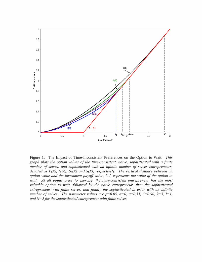
0
0.2
0.4
0.6
0.8
1
1.2
1.4
1.6
1.8
2
0 0.5 1 1.5 2 2.5 3
Payoff Value X
Opt
ion
Valu
es
V(X)
N(X)
S(X)
S0(X)
X-I
X*XNaiveXS XS,0
Figure 1: The Impact of Time-Inconsistent Preferences on the Option to Wait. This graph plots the option values of the time-consistent, naive, sophisticated with a finite number of selves, and sophisticated with an infinite number of selves entrepreneurs, denoted as V(X), N(X), S0(X) and S(X), respectively. The vertical distance between an option value and the investment payoff value, X-I, represents the value of the option to wait. At all points prior to exercise, the time-consistent entrepreneur has the most valuable option to wait, followed by the naive entrepreneur, then the sophisticated entrepreneur with finite selves, and finally the sophisticated investor with an infinite number of selves. The parameter values are ρ=0.05, α=0, σ=0.35, δ=0.90, λ=5, I=1, and N=5 for the sophisticated entrepreneur with finite selves.
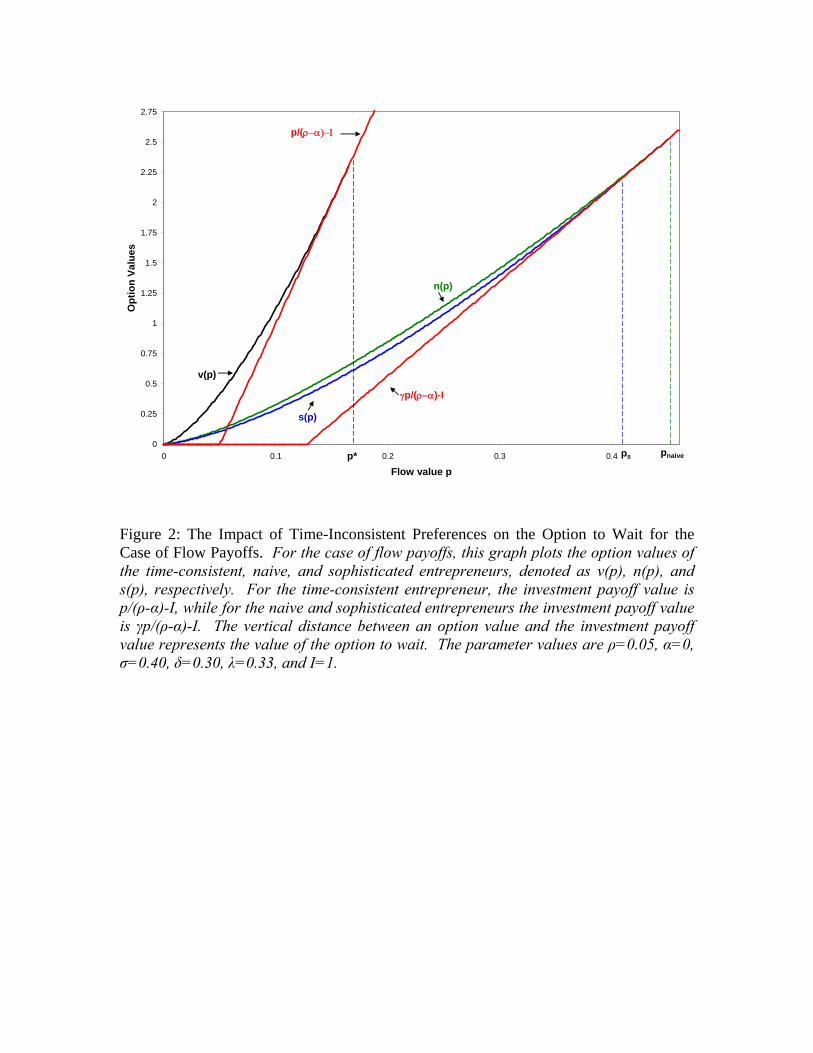
0
0.25
0.5
0.75
1
1.25
1.5
1.75
2
2.25
2.5
2.75
0 0.1 0.2 0.3 0.4
Flow value p
Opt
ion
Valu
esp/(ρ−α)−Ι
s(p)
n(p)
v(p)
γp/(ρ−α)-I
p* ps pnaive
Figure 2: The Impact of Time-Inconsistent Preferences on the Option to Wait for the Case of Flow Payoffs. For the case of flow payoffs, this graph plots the option values of the time-consistent, naive, and sophisticated entrepreneurs, denoted as v(p), n(p), and s(p), respectively. For the time-consistent entrepreneur, the investment payoff value is p/(ρ-α)-I, while for the naive and sophisticated entrepreneurs the investment payoff value is γp/(ρ-α)-I. The vertical distance between an option value and the investment payoff value represents the value of the option to wait. The parameter values are ρ=0.05, α=0, σ=0.40, δ=0.30, λ=0.33, and I=1.
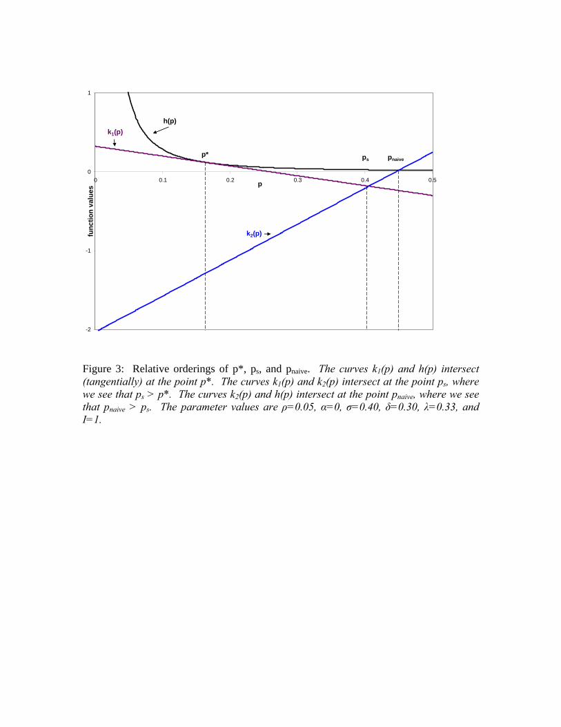
-2
-1
0
1
0 0.1 0.2 0.3 0.4 0.5p
func
tion
valu
es
h(p)k1(p)
k2(p)
p* ps pnaive
Figure 3: Relative orderings of p*, ps, and pnaive. The curves k1(p) and h(p) intersect (tangentially) at the point p*. The curves k1(p) and k2(p) intersect at the point ps, where we see that ps > p*. The curves k2(p) and h(p) intersect at the point pnaive, where we see that pnaive > ps. The parameter values are ρ=0.05, α=0, σ=0.40, δ=0.30, λ=0.33, and I=1.


