NBER WORKING PAPER SERIES
REDISTRIBUTION BY INSURANCE MARKET REGULATION:ANALYZING A BAN ON GENDER-BASED RETIREMENT ANNUITIES
Amy FinkelsteinJames Poterba
Casey Rothschild
Working Paper 12205http://www.nber.org/papers/w12205
NATIONAL BUREAU OF ECONOMIC RESEARCH1050 Massachusetts Avenue
Cambridge, MA 02138April 2006
We are grateful to Jeff Brown, Pierre-Andre Chiappori, Keith Crocker, Peter Diamond, Liran Einav, MikhailGolosov, Robert Gibbons, Kenneth Judd, Whitney Newey, Bernard Salanie, and participants at the NBERInsurance Meeting, the Stanford Institute for Theoretical Economics, and the Econometric Society AnnualMeeting for helpful discussions, to Luke Joyner and Nelson Elhage for research assistance, and to theNational Institute of Aging and the National Science Foundation (Poterba and Rothschild) for researchsupport. The views expressed herein are those of the author(s) and do not necessarily reflect the views of theNational Bureau of Economic Research.
©2006 by Amy Finkelstein, James Poterba and Casey Rothschild. All rights reserved. Short sections of text,not to exceed two paragraphs, may be quoted without explicit permission provided that full credit, including© notice, is given to the source.

Redistribution by Insurance Market Regulation: Analyzing a Ban on Gender-Based RetirementAnnuitiesAmy Finkelstein, James Poterba and Casey RothschildNBER Working Paper No. 12205April 2006JEL No. D82, H55, L51
ABSTRACT
This paper shows how models of insurance markets with asymmetric information can be calibratedand solved to yield quantitative estimates of the consequences of government regulation. Weestimate the impact of restricting gender-based pricing in the United Kingdom retirement annuitymarket, a market in which individuals are required to annuitize tax-preferred retirement savings butare allowed considerable choice over the annuity contract they purchase. After calibrating a lifecycleutility model and estimating a model of annuitant mortality that allows for unobserved heterogeneity,we solve for the range of equilibrium contract structures with and without gender-based pricing.Eliminating gender-based pricing is generally thought to redistribute resources from men to women,since women have longer life expectancies. We find that allowing insurers to offer a menu ofcontracts may reduce the amount of redistribution from men to women associated with gender-blindpricing requirements to half the level that would occur if insurers were required to sell a singlepre-specified policy. The latter "one policy" scenario corresponds loosely to settings in whichgovernments provide compulsory annuities as part of their Social Security program. Our findingssuggest that recognizing the endogenous structure of insurance contracts is important for analyzingthe economic effects of insurance market regulations. More generally, our results suggest thattheoretical models of insurance market equilibrium can be used for quantitative policy analysis, notsimply to derive qualitative findings.
Amy FinkelsteinDepartment of EconomicsMIT E52 262F50 Memorial DriveCambridge MA 02142and [email protected]
James M. PoterbaDepartment of EconomicsMIT, E52-35050 Memorial DriveCambridge, MA 02142-1347and [email protected]
Casey RothschildMIT Department of EconomicsOffice Number E51-390E52, Room 391Cambridge MA 02142-1347 [email protected]

1
Restrictions on the use of characteristics such as race or gender in pricing are ubiquitous in private
insurance markets. These restrictions are likely to become even more important as the advent of genetic
tests enriches the information set that insurers might use to price life and health insurance policies.
Several theoretical studies, including Hoy (1982) and Crocker and Snow (1986), have analyzed this form
of regulation and shown qualitatively that they have unavoidable negative efficiency consequences.
Empirical work such as Buchmueller and DiNardo (2002) and Simon (forthcoming) has confirmed the
existence of such efficiency costs by documenting declines in insurance coverage when characteristic-
based pricing is banned in health insurance markets. However, there have been few if any attempts to
develop quantitative estimates of the efficiency costs or the distributional impacts of restrictions on
characteristic-based pricing. One of the few studies in this vein is Blackmon and Zeckhauser’s (1991)
analysis of automobile insurance regulation. It frames questions similar to the ones we study but does not
analyze how the structure of insurance contracts may respond to regulatory restrictions or how this affects
distributional or efficiency effects.
In this paper, we take a first step toward developing quantitative estimates of the effects of
endogenous contract responses to insurance market regulation. We extend existing theoretical models and
adapt them to provide quantitative estimates of both the efficiency and redistributive effects of a unisex
pricing requirement for pension annuities. Restrictions on characteristic-based pricing are usually thought
to transfer resources from individuals in lower-risk categories to those with greater risks. Women are
longer-lived than men, so unisex pricing restrictions in the pension marketplace redistribute from men to
women. Some might argue for such policies on redistributive grounds, since elderly women have higher
poverty rates than elderly men. Viewed from the ex-interim perspective once individual characteristics
are known, the transfers from men to women generate redistribution akin to the redistribution associated
with uniform pricing regulations in industries such as telephone and electricity distribution, where
individuals have different costs of service. Posner (1971) labeled such redistribution “taxation by
regulation.” Alternatively, from an ex-ante perspective before individual characteristics are known, the

2
redistribution may be viewed as a form of insurance against drawing a high-cost characteristic, in this
case being female, as in Hirshleifer (1971).
In addition to providing a tractable setting for illustrating our techniques, the pension annuity market
is an interesting setting in its own right because of its size, its importance for retiree welfare, and the
salience of unisex pricing regulations in this market. Private annuity arrangements, typically the payouts
from defined benefit pension plans, represent an important source of retirement income for many elderly
households. Employers in the United States were once free to offer different pension annuity payouts to
men and women, but litigation in the 1970s and early 1980s eliminated this practice. The European Union
is currently debating regulatory reforms that may eliminate gender-based pricing in insurance markets,
including pension annuity markets. Our analysis may also have broader implications for the design and
regulation of annuitized payout structures associated with defined contribution Social Security systems.
We are not aware of any previous attempts to calibrate and solve stylized theoretical models of
insurance market equilibria. Doing so requires adapting these models to account for a number of features
that are observed in actual insurance markets. One that has quantitatively important implications is our
relaxation of the assumption that individuals have no recourse to an informal, if inefficient, substitute for
insurance. Our analysis recognizes that individuals may save against the contingency of a long life, and
that insurance companies many not observe savings by their policyholders. If we do not allow for
unobservable savings, the informational asymmetries created by a ban on gender categorization may have
neither efficiency nor distributional effects.
We focus on the retirement annuity market in the United Kingdom, where we have obtained a rich
micro-data set that facilitates our calibration. A critical feature of this market is that workers who have
accumulated tax-preferred retirement savings must purchase an annuity. They cannot choose whether or
not to participate in the annuity market, which eliminates one margin on which unisex pricing regulations
could potentially affect individual behavior. Participants do have substantial flexibility with regard to
contract choice. Empirical evidence, such as that presented in Finkelstein and Poterba (2004), suggests
that this choice is affected by private information about risk type.

3
Our main finding is that recognizing the endogenous response in the structure of insurance contracts
when regulations change may reduce by as much as fifty percent the amount of redistribution away from
men and toward women that would be associated with a ban on gender-based annuity pricing in a fully
compulsory annuity market with no scope for this response; this latter setting in which insurers are
required to sell a single pre-specified policy loosely corresponds to settings in which governments provide
compulsory annuities as part of their Social Security program. Our findings highlight the importance of
recognizing the endogenous structure of insurance contracts when analyzing the economic effects of
insurance market regulation, and they indicate that theoretical models of insurance market equilibrium
can be adapted to offer quantitative predictions on regulatory issues. Even accounting for the endogenous
contract response, however, we find that a ban on gender-based pricing in the U.K. retirement annuity
market would have substantial distributional consequences, in most cases redistributing at least three
percent of retirement wealth from men to women. We also estimate that the efficiency costs associated
with this redistribution would be very small. However, since individuals do not have a choice of whether
or not to participate in this market, our estimates of the efficiency costs of unisex pricing restrictions are
likely to substantially underestimate the cost of such restrictions in voluntary annuity markets.
Our analysis is divided into six sections. The first briefly reviews the qualitative impact of uniform
pricing requirements in insurance markets with asymmetric information. Based on the assumption that
annuity markets operate in a constrained-efficient manner, section two develops a model of the range of
possible contracts offered and purchased in equilibrium. It also describes results concerning equilibrium
contract structure and our algorithm for solving for these contracts. It is supplemented by a technical
appendix. In the third section we calibrate the model and describe our estimates of a two-type mixture
model for mortality rates. Section four describes the measures that we use for evaluating the efficiency
and distributional effects of policy interventions in insurance markets. The fifth section presents our
quantitative results. We describe the range of possible distributional and efficiency effects of restrictions
on gender based pricing under different assumptions concerning the constraints on consumers and

4
producers. A brief conclusion discusses how our results bear on a number of ongoing policy debates and
describes possible generalizations of our approach to other insurance markets.
1. A Framework for Analyzing Regulation in Insurance Markets
This section reviews the qualitative efficiency and distributional effects of a ban on categorization in
a standard two-state, two-type model of competitive insurance markets with asymmetric information.
This framework considers two distinct types of individuals who are indistinguishable to an insurance
company but who face different risks of a loss. Individuals can insure themselves against loss by
purchasing a single insurance contract from firms in a competitive market.
1.1 Qualitative Analysis of Banning Categorization in the “Perfect Categorization” Case
There is little consensus concerning the proper equilibrium concept for insurance markets with
asymmetric information, as Hellwig (1987) explains. We therefore follow the approach taken by Crocker
and Snow (1986) in their analysis of the efficiency impacts of bans on categorization and focus on
constrained efficient outcomes. In focusing on these outcomes, we implicitly assume that the private
market achieves efficient outcomes, within the scope of their ability to do so, without explicitly modeling
equilibrium behavior. We note, however, that the so-called Miyazaki (1977)-Wilson (1977)-Spence
(1978) (hereafter MWS) equilibrium provides an example of a model of equilibrium behavior that results
in a constrained efficient outcome. We will describe this MWS outcome in more detail after
characterizing the entire efficient frontier, as it will play an important role in our analysis.
To characterize the frontier, denote the high risk and low risk types by H and L, respectively. Let
)(AV i denote the indirect utility achieved by type i when she has purchased insurance contract A, and let
)(AiΠ denote the expected profits a firm earns by selling contract A to type i. With this notation, points
on the Pareto frontier solve the following program, where λ is the proportion of H types:

5
(1)
,0)()()1()()()(
)()()(
)()()(
)(max,
≥Π+Π−
≥
≥
≥
HHLL
HHH
HLLLL
LHHHH
LL
AA
AABCVAVMU
AVAVIC
AVAVICtosubject
AVHL
λλ
where (ICi) is the incentive compatibility constraint stating that i types must be willing to choose the
contract designed for them, (BC) is a budget constraint that requires that on average policies break even,
and (MU) is a minimum utility constraint for the H types.
Crocker and Snow (1985) characterize this constrained Pareto frontier in the standard two period
(one-accident) setting by varying the Lagrange multiplier on constraint (MU) in (1). In Figure 1, we
characterize the frontier in the same two-period setting by varying the value of HV . Insurance contracts
can be written as state-contingent consumption vectors ),( 10 aaA = , where the subscript 0 refers to the
“no accident” state and the subscript 1 refers to the “accident” state. Insurance providers supply these
consumption promises A in exchange for a buyer’s state-contingent endowment wealth vector
),( 00 l−= wwW . H types have a higher probability of experiencing state 1 and the types are otherwise
identical expected utility maximizers with a strictly concave utility function.
For low values of HV , (MU) may be slack. For example, if { }
)(max0)(:
AVV H
AA
HH =Π
= so that (MU)
says that H types have to be at least as well off as they would be with their full insurance actuarially fair
consumption point, then (MU) will be slack precisely when the Rothschild and Stiglitz (1976) equilibrium
either fails to exist or exists but fails to be constrained efficient. Such a situation is depicted at point M in
Figure 1. At point M, L types consume the constrained efficient allocation that is best for them; this
corresponds to the MWS equilibrium. Figure 1 shows that even this best-for-L allocation can involve
positive cross subsidies from the Ltypes to the H types.

6
The dark curve connecting points M and F in Figure 1 depicts a portion of the locus of the L type
consumption points that correspond to constrained Pareto optimal outcomes. The point labeled F is the
unique “pooling” outcome on the frontier – i.e., the unique constrained efficient outcome with HL AA = .
It is on the 45-degree line and therefore provides full insurance. Point F involves substantially larger
cross subsidies from L types to H types than does M. There are additional constrained efficient outcomes
not depicted in Figure 1 which involve even larger cross subsidies from L type to H types than those at
point F. Such outcomes involve the L types being fully insured and the H types being overinsured, which
Crocker and Snow (1985) note is a feature absent from standard models of equilibrium in insurance
markets. As a result, we do not consider this portion of the frontier. The set of outcomes we consider is
thus captured in the region of the frontier bounded by F and M; we do not try to select any particular
constrained efficient outcome from this set.
Because (1) permits – and, as in the case of Figure 1, may even require – the market to implement a
contract pair involving cross subsidies across types, bans in characteristic-based pricing can have both
distributional and efficiency consequences. This is illustrated in Figure 2, which depicts a constrained
efficient pair of contracts. When type is observable and can be used in pricing, the competitive
equilibrium will provide each type with her actuarially fair full insurance contract. In Figure 2, *HA and
*LA depict the full insurance actuarially fair contracts that we assume emerge when type is observable
and can be contracted upon. Consumption for each type is independent of the realized state of nature.
When type-based pricing is banned, our assumption is that the market implements a pair of contracts,
labeled HA and LA , which is constrained efficient given the informational restrictions of the ban. Note
that as depicted this contract pair involves positive cross subsidies between types. As a result, H types are
better off when categorization is banned, and L types are worse off. This illustrates how a ban on
categorical-based pricing may have distributional consequences. The ban is efficiency reducing in this
example as well. Since type is, in fact, observable, it is in principle possible to make L types as well off
as with LA via contract LA′ , which is also actuarially cheaper to provide to the L types.
7
1.2 Residual Private Information
The foregoing discussion assumes that type is observable. A ban on characteristic-based pricing
therefore moves the economy from perfect information to imperfect information. In practice, information
such as gender or the outcome of a genetic test may be related to risk type, but even conditional on this
information, insurers are unlikely to be able to completely determine the risk of potential policy buyers.
The relevant comparison is therefore between imperfect information and more imperfect information.
Our study builds on previous analyses of bans on characteristic-based pricing, such as Hoy (1982)
and Crocker and Snow (1986), which use the most parsimonious model that can capture the presence of
residual uncertainty. There are still two risk types, but risk type is not directly observable. Instead,
insurers only observe a signal that is correlated with risk type. There are two possible signals, X and Y.
We henceforth refer to individuals as falling in category X or category Y. A fraction kλ of category k
individuals are high risk types, with .10 <<< YX λλ Thus, category Y is the high-risk category, but
there are still low-risk types within that category. We denote by θ the fraction of category Y individuals
in the population.
For our analysis, we continue to assume that markets will operate in a constrained efficient manner
given the information which is both available and legal for use in pricing. When characteristic-based
pricing is permitted, we further assume that the market will not implement contracts involving cross-
subsidies across observable categories, just as we did in Figure 2 by assuming that the contracts *HA and
*LA emerge when type-based pricing was allowed. A ban on categorical pricing in this imperfect-
information setting will have the same qualitative effects as it does in the perfect information setting
described above.
2. Modeling Restrictions on Gender-Based Pricing in the U.K. Pension Annuity Market
The preceding discussion illustrates the qualitative impact of a ban on categorization on efficiency
and redistribution. To develop quantitative estimates, we consider a particular ban on categorization in a
8
particular market, namely the imposition of unisex pricing requirements in the U.K. annuity market.
Individuals in the United Kingdom with defined contribution private pension plans that have benefited
from tax deferral on investment income—the analogues of IRAs and 401(k)’s in the United States—face
compulsory annuitization requirements for a substantial share of the balance accumulated by retirement.
In 1998, data from the Association of British Insurers (1999) suggest that annual annuity payments in this
market totaled £5.4 billion.
Although annuitization is compulsory, annuitants in the U.K. retirement annuity market have some
scope for self-selection across contract choice. Finkelstein and Poterba (2004, 2006) find that such self-
selection appears to reflect private information about mortality risk. Note that, from the perspective of an
insurance company, high-risk annuitants are those who are likely to live longer than the characteristics
used in pricing, such as age and gender, would suggest. There are currently no regulations in the U.K.
annuity market limiting the characteristics used in pricing annuities. In practice, annuities are priced
almost exclusively on age at purchase and gender. Several small firms entered the annuity market after
the end of our sample with discounted annuities for heavy smokers, but those products were not available
during the period that we study.
While the two-state model discussed above suffices for the understanding the qualitative impacts of
interventions that ban categorical pricing, it is too stylized to plausibly measure the quantitative impact of
regulatory interventions. Since an individual can live for many years after the purchase of their annuity,
we extend the analysis to 35 periods. Boadway and Townley (1988) is the only other contract theoretic
model we have found that includes more than three periods in an analysis of an annuity market with
asymmetric information, but the contracts under consideration have a particular and restrictive form that
we relax. This extension to many periods is essential for a plausible calibration.
Our baseline model also allows for unobservable savings. Eichenbaum and Peled (1987), Brunner and
Pech (2005), and others note that allowing annuitants to engage in unobservable saving limits the ability
of insurers to screen different types of observationally equivalent annuity buyers. In our context, we show
that when insurance companies can observe savings, the informational asymmetries created by a ban on

9
gender categorization can have neither efficiency nor distributional consequences. The process of
deriving and solving the model, which we discuss below, provides insight into why accounting for
unobservable savings is critical for any plausible calibration. It also demonstrates why this extension
makes the model substantially more difficult to solve. We show that it is nevertheless possible to solve for
the contracts on the constrained Pareto frontier, and we sketch our computational algorithm.
2.1 Defining Annuity Market Outcomes
Our model applies to any number of periods Nt ,,0 L= , where we interpret t as the number of years
after retirement, which we take to be at age R=65. In practice, we take N=35, thereby assuming
individuals do not live past age 100. To capture the compulsory purchase requirement, we assume that
individuals must use their retirement wealth W to purchase an annuity. They exponentially discount the
future at rate r+= 11δ per year, where r is the interest rate, and by their (cumulative) probability tS of
living to a given age R+t. The two risk types, H and L, differ only in their survival probabilities. There is
a continuum of individuals, with a fraction λ of H types. We assume Lt
Lt
Ht
Ht
SS
SS 11 ++ > for each t; in other
words, the ratio of the cumulative survival probabilities of the two types must be monotone in age. This
is satisfied if the higher longevity type has a lower mortality hazard at every age.
The direct utility of a consumption stream ( )Ncc ,,0 L=Γ for type σ is given by:
(3) ∑∑=
−
= −==
N
t
tt
tN
ttt
tN
cScuSccU
0
1
00 1
)(),,(γ
δδγ
σσσ L ,
where γ is the risk-aversion parameter. Annuity streams, which are denoted by A, specify a life-
contingent payment ta in each of the N +1 periods. In our baseline model, we impose no structure on the
annuity payments ta ; we later restrict the time profile of possible annuity payments.
Individual savings earn an interest rate r. Individuals have no bequest motive, and they cannot borrow
against their annuity. This means that individuals with an annuity stream A can obtain any consumption

10
stream that satisfies ⎭⎬⎫
⎩⎨⎧
∀≤Γ≡∈Γ ∑∑ tacAFt
ss
t
ss
00)( δδ . This induces indirect utility functions and
type-specific actuarial cost functions
(4) )(max)()(
Γ=∈Γ
σσ UAVAF
,
and
(5) ∑≡N
ttn aSAC
0
)( σσ δ .
Because individuals discount the future at the rate of interest, “full insurance” annuities have level real
payouts. Let )(XV σ denote the utility that type σ gets by consuming the full insurance annuity A
with XAC =)(σ . Let λA denote the pooled-fair full insurance annuity – i.e., the full insurance annuity
satisfying WACAC LH =−+ )()1()( λλ λλ . In a constrained efficient market, the two risk types
purchase a pair of annuities HA and LA that solve:
(6)
WACACBCVAVMU
AVAVIC
AVAVICtosubject
AV
HHLL
HHH
HLLLL
LHHHH
LL
AA HL
≤+−
≥
≥
≥
)()()1()()()(
)()()(
)()()(
)(max,
λλ
for some HV . We further assume that )()( λAVVWV HHH ≤≤ , so that H types are at least as well
off as they would be if they revealed their type, and are no better off than they would be under a pooled-
fair full insurance outcome. This range corresponds with the portion of the efficient frontier in Figure 1.
Solving (6) is non-trivial: it involves solving for the N +1 year-specific annuity payments for each of the
two types. Furthermore, the functions )(AV σ are themselves implicitly defined via (4), which is an
optimization problem over N +1 variables. Nevertheless, (6) is computationally tractable.
11
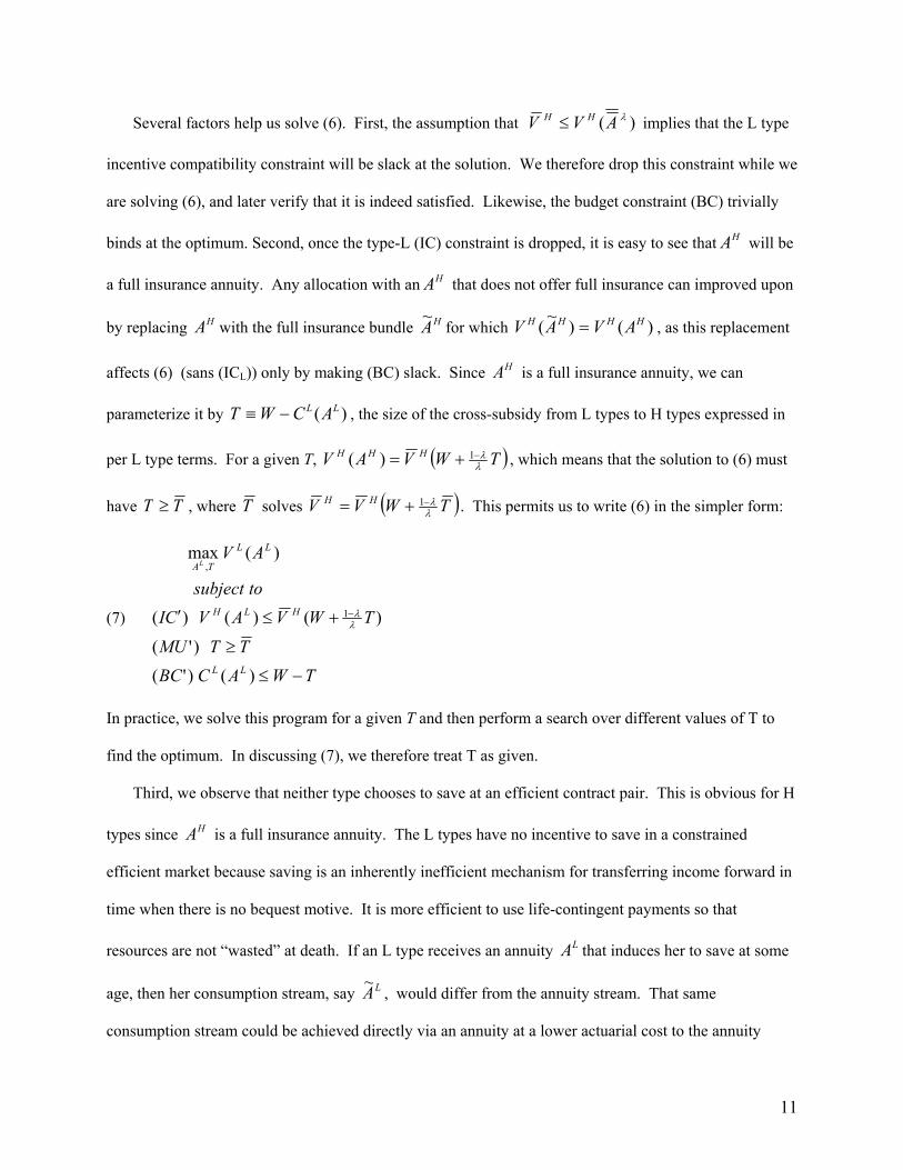
Several factors help us solve (6). First, the assumption that )( λAVV HH ≤ implies that the L type
incentive compatibility constraint will be slack at the solution. We therefore drop this constraint while we
are solving (6), and later verify that it is indeed satisfied. Likewise, the budget constraint (BC) trivially
binds at the optimum. Second, once the type-L (IC) constraint is dropped, it is easy to see that HA will be
a full insurance annuity. Any allocation with an HA that does not offer full insurance can improved upon
by replacing HA with the full insurance bundle HA~ for which )()~( HHHH AVAV = , as this replacement
affects (6) (sans (ICL)) only by making (BC) slack. Since HA is a full insurance annuity, we can
parameterize it by )( LL ACWT −≡ , the size of the cross-subsidy from L types to H types expressed in
per L type terms. For a given T, ( )TWVAV HHHλλ−+= 1)( , which means that the solution to (6) must
have TT ≥ , where T solves ( )TWVV HHλλ−+= 1 . This permits us to write (6) in the simpler form:
(7)
TWACBCTTMU
TWVAVCItosubject
AV
LL
HLH
LL
TAL
−≤
≥
+≤′ −
)()'()'(
)()()(
)(max
1
,
λλ
In practice, we solve this program for a given T and then perform a search over different values of T to
find the optimum. In discussing (7), we therefore treat T as given.
Third, we observe that neither type chooses to save at an efficient contract pair. This is obvious for H
types since HA is a full insurance annuity. The L types have no incentive to save in a constrained
efficient market because saving is an inherently inefficient mechanism for transferring income forward in
time when there is no bequest motive. It is more efficient to use life-contingent payments so that
resources are not “wasted” at death. If an L type receives an annuity LA that induces her to save at some
age, then her consumption stream, say LA~ , would differ from the annuity stream. That same
consumption stream could be achieved directly via an annuity at a lower actuarial cost to the annuity
12
provider. There is therefore some surplus to be created by reducing the annuity’s payouts in its early
years and raising its payouts in later years. Insurers in an efficient market will take advantage of such
opportunities to repackage the timing of cash flows until the surplus is eliminated and L types no longer
wish to save from the annuity. Formally, consider replacing LA with LA~ in (7). L types would be
exactly as well off as before, but when LL AA ~≠ the budget constraint would be made strictly looser.
Furthermore, the incentive compatibility constraint will be no tighter, and possibly strictly looser, as a
result of the replacement. Therefore, LA can only solve (7) when LL AA ~= .
The observation that neither type chooses to save means that, in equilibrium, )()( LLLL AUAV = and
)()( HHHH AUAV = , so both can be computed directly instead of by solving the non-trivial (4). The
only part of (7) that is difficult to compute is )( LH AV , the utility that H types get if they deviate to
purchasing the L type annuity and saving optimally. The structure of (7) in fact allows us to evaluate
)( LH AV in solving for equilibrium without explicitly solving (4). In particular, with the parametric forms
we assume on the survival probabilities and preferences, );(~)( *nAVAV LHLH = at any solution to (7)
for some n*, where
(8) ∑=
=N
t
Ht
Ht
tL
H cuSnAV0
* )~();(~ δ
and where
(9)
⎪⎪⎪
⎭
⎪⎪⎪
⎬
⎫
⎪⎪⎪
⎩
⎪⎪⎪
⎨
⎧
≥
⎟⎟⎠
⎞⎜⎜⎝
⎛
⎟⎟⎠
⎞⎜⎜⎝
⎛
<
=
∑
∑
=
=*
*
*
1
*
*
1
*
~
ntif
SS
aSS
ntifa
c
Nnn H
n
Hnn
Nnn
Ln
nHn
Ht
Lt
Ht
γ
γ
δ
δ
Equations (8) and (9) describe the utility achieved by an H type with an annuity stream LA when she
consumes the payments before period n*, and thereafter follows the consumption pattern she would
13
follow if the remaining annuity stream ( )LN
Ln
aa ,,* L were a bond against which she could save and
borrow at the constant rate r. Hence, saying that );(~)( *nAVAV LHLH = for some n* at a solution to (7)
is tantamount to saying that that the optimal consumption pattern of H types who deviate and buy annuity
stream LA is of this form. Note that for their utility to be given by a consumption pattern of this form, the
stream LA must be such that this consumption pattern of deviating H types does not involve borrowing.
The formal proof that annuity stream LA has the property that deviating H types will optimally
consume in accord with (9) is shown in the appendix. The intuition is relatively straightforward,
however, and it offers insights into the critical importance of saving in determining the optimum annuity
streams. Suppose that annuitants could not save. Then we could find the solution to (7) by simply
replacing )( LH AV with )( LH AU . This modified program could be solved using first order conditions.
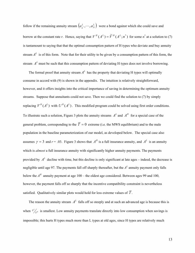
To illustrate such a solution, Figure 3 plots the annuity streams LA and HA for a special case of the
general problem, corresponding to the 0=T extreme (i.e. the MWS equilibrium) and to the male
population in the baseline parameterization of our model, as developed below. The special case also
assumes 3=γ and r = .03. Figure 3 shows that HA is a full insurance annuity, and LA is an annuity
which is almost a full insurance annuity with significantly higher annuity payments. The payments
provided by LA decline with time, but this decline is only significant at late ages – indeed, the decrease is
negligible until age 97. The payments fall off sharply thereafter, but the AL annuity payment only falls
below the AH annuity payment at age 100 – the oldest age considered. Between ages 99 and 100,
however, the payment falls off so sharply that the incentive compatibility constraint is nevertheless
satisfied. Qualitatively similar plots would hold for less extreme values of .T
The reason the annuity stream LA falls off so steeply and at such an advanced age is because this is
when HL
SS is smallest. Low annuity payments translate directly into low consumption when savings is
impossible; this hurts H types much more than L types at old ages, since H types are relatively much

14
more likely to still be alive. In other words, the best way from the perspective of L types to satisfy
incentive compatibility for H types involves providing a downward tilt at extreme old ages, when the
relative probability of L types being alive, compared to H types, is lowest.
When savings is possible, such a steep drop-off is far less useful as a self-selection device because it
can always be undone – albeit inefficiently – by saving. Indeed, Figure 3 also shows the optimal
consumption pattern Htc~ and bond-wealth holding of H types who receive annuity LA but who can also
save. These H types optimally choose to consume the annuity payments until age 96, after which they use
their savings to smooth out the sharp drop-off in the annuity stream. Because such saving reduces the
power of downward-sloping payout schedules as a selection device, when savings is possible, the
extremely sharp fall-off of payments LA will no longer be optimal. However, the incentive for positive
saving by deviating H types will still be as in (9).
2.2 Optimal Structure of Contracts
A central contribution of our modeling is finding the optimal structure of annuity contracts when
annuitants can save. This involves solving (7). We cannot offer general analytic solutions, so our
findings necessarily require assumptions about the underlying functional forms of the utility function, the
mortality rates, and other parameters. Using the same baseline parameters that we used in Figure 3, and
the same assumption that 0=T , Figure 4 plots the solution to (7) and shows the actuarially fair full
insurance annuities for both H type and L type individuals, as well as the optimal consumption stream of
an H type who deviates and purchases annuity LA . Again, qualitatively similar graphs would obtain for
other values of .T
Several features of Figure 4 are worthy of note. First, the solution involves substantial cross-
subsidies. This is clear from the comparison of the level of the H type fair level annuity and the H type
optimum annuity HA , as HA offers strictly higher payouts. Second, while LA provides a downward
sloping annuity stream, it declines much more gradually than the annuity stream shown in Figure 3,
which corresponded to the case in which annuitants could not save. Third, comparison of the optimal
15
consumption stream of an H type deviating to LA reveals that the deviating H type who purchases LA
will immediately begin to save. In the notation above, this means 0* =n in (8) and (9).
Comparison of Figures 3 and 4 shows the important effect of allowing for unobservable saving on the
structure of the optimal annuity streams. Though it is more difficult to find the optimal annuities with
unobservable saving than without, the evident realism that allowing for such saving provides leads us to
choose this as our benchmark case. Indeed, the results in Figure 3 suggest that if unobservable saving is
not possible, asymmetric information is essentially irrelevant because the optimal annuity streams are
virtually identical to the annuity streams that would obtain with symmetric information. The findings
more generally suggest caution in using applied contract theoretic models for quantitative purposes when
there are inefficient and unobservable behaviors the insured can undertake as a substitute for formal
insurance.
2.3 Discussion of Key Assumptions
The importance of unobservable savings highlights one of several extensions we have made to the
standard stylized model of insurance markets with asymmetric information. These extensions provide a
more realistic framework for analyzing the impact of a ban on gender-based pricing. Nonetheless, the
model that we develop in (6) and (7), and then solve, makes a number of assumptions for tractability.
Some – such as the use of constant relative risk aversion utility or the assumption that individuals
discount the future at the rate of interest – are standard. It is worth, however, briefly commenting on
several that are more specific to this application.
First, we have not incorporated bequest motives into our model. The importance of bequests in
explaining saving behavior has been widely debated, for example by Kotlikoff and Summers (1981),
Hurd (1987, 1989), Bernheim (1991), and Brown (2001), but no consensus has emerged. Conceptually,
the presence of bequest motives can easily be incorporated into our framework. We would simply add
utility from consumption in states when the consumer is dead. Since our solution algorithm relies heavily
on the shape of preferences, however, this extension can pose practical issues of computational
16
tractability. In part for this reason, we have addressed the analytically more convenient setting without
bequests, while recognizing that this limits the applicability of our findings if actual consumption
decisions are substantially affected by bequest motives.
Second, we have followed previous theoretical models, notably Hoy (1982) and Crocker and Snow
(1986), in modeling mortality heterogeneity via two risk types. The computational challenge of finding
optimal contracts is much more difficult in a many-type setting, although similar solution algorithms to
the ones we developed here would, in principle, also apply. We show below that our data cannot reject
this parsimonious model in favor of one which allows the underlying types to differ by gender.
Finally, we emphasize more generally that while our model incorporates some important features of
the U.K. annuity market, it does not capture many others. For example, we focus on single life annuities,
and we ignore individuals’ option to purchase limited term guarantees of their contracts. We also ignore
the presence of wealth outside the retirement accounts. We abstract from the possible presence of risks
other than longevity risk, such as liquidity risks or health shocks; Crocker and Snow (2005) discuss how
the existence of such “background risks” can affect the insurance market equilibrium. Finally, our model
does not allow for the possibility of individuals learning over time about their risk type; Polborn et al.
(2004) show that allowing for such dynamic considerations in a model in which individuals have
flexibility in the timing of their insurance purchases can have important qualitative effects for the impact
of restrictions on characteristic-based pricing. In part because of these and other abstractions, the optimal
annuity contracts we compute do not match the actual contracts observed in the data; we discuss this in
more detail below.
3. Model Calibration
Calibrating our model to yield quantitative estimates of the efficiency and distributional consequences
of mandating unisex prices requires the constant relative risk aversion parameter γ; the real interest rate r;
the fraction of high risk individuals among men ( Mλ ) and among women ( Fλ ); the fraction θ of women

17
in the relevant population; and the survival curves for each risk type ) and ( LH SS . We present results
for risk aversion coefficients of 1, 3 and 5. We assume the interest rate r is equal to 0.03 and set the
discount rate r+= 11δ . We set 5.0=θ in our baseline case, but we also report results for other values.
We jointly estimate the remainder of the parameters using micro-data on a sample of compulsory
annuitants who bought annuities from a large U.K. life insurance company between 1981 and 1998. We
have information on their survival experience through the end of 1998. These data, which are described in
more detail in Finkelstein and Poterba (2004), appear to be reasonably representative of the U.K. annuity
market. We restrict our attention to annuities that insure a single life, as opposed to joint life annuities
that continue to pay out as long as one of several annuitants remains alive. In addition, we focus on
individuals who purchased annuities at the modal age for men (age 65). We exclude annuitants who died
before their 66th birthday and consider only mortality after age 66, so that we have a uniform entry age.
Our final sample consists of 12,160 annuitants of whom 1,216 are women; this represents about a third of
the single-life sample of all ages analyzed in Finkelstein and Poterba (2004).
We estimate the survival curves for two underlying, unobserved risk types H and L. Our approach, in
the spirit of Heckman and Singer (1984), is to assume a parametric form for the baseline mortality hazard,
and to jointly estimate the parameters of the baseline and the two multiplicative parameters that capture
the unobserved heterogeneity. We follow the actuarial literature on mortality modeling, such as Horiuchi
and Coale (1982), and assume a Gompertz functional form for the baseline hazard. This is particularly
well suited to our context because our data are sparse in the tails of the survival distribution. Formally,
for a given risk typeσ , the mortality hazard at age ix is given by:
(10) ))(exp()( bxx ii −⋅= βασμ σ ,
where b is the base age, 65 in our case. We assume that the growth parameter β is common to both risk
types and to both genders. This means that β determines the shape of the mortality curves for both types,

18
which differ only in the values of σα . Using the notation bxt ii −= , this form of the hazard implies
risk-type-specific survival function of the form:
(11) ⎭⎬⎫
⎩⎨⎧
⋅−= ))exp(1(exp)( ii ttS ββα
σ σ .
When the two underlying risk types are the same for males and females, so that only the mix of these two
risk types is allowed to differ across genders, our stochastic model depends on a parameter vector Θ =
{ Lα , Hα , β , fλ , mλ }. The likelihood function in this case will be:
(12)
( ) ( )
},{)),,|()1()(,|(
)1(1)1(1)(
LHtddtSlwhere
llllL
iiii
i
Lif
Hifm
Lim
Himm
=−+=
−+⋅+−+⋅≡Θ ∑
σβαμβα
λλλλ
σσσσ
In (12), the variable id is an indicator for whether the individual observation is censored and 1m and
1f are indicator variables for whether an individual is male or female respectively. An individual’s
contribution to the likelihood function is a weighted average of the likelihood function of a high risk and
low risk type, with the weights equal to the gender-specific fraction of high and low risk individuals.
Eighty-one percent of the observations in our sample are censored because the annuitant is still alive at
the end of the sample period, December 31, 1998.
Table 1 presents our estimates of the mortality model in (11) and (12). Our estimates yield aggregate
mortality statistics that are similar to those published by the Institute of Actuaries (1999) for all 65 year-
old U.K. pensioners in 1998. For example, the life expectancies implied by our model differ from those
in the aggregate tables by only 0.26 years for women and 0.45 years for men. The estimates of the
mortality rates for the high risk and the low risk types are quite far apart, implying large differences in life
expectancies. For example, the estimates in Table 1 imply that life expectancy at 65 is only 8.8 years for
low risk types, compared to 23.2 for high risk types. Column 5 indicates that over 80 percent of women
are classified in the high risk (long-lived) group, compared to only about 60 percent of men (column 4).
As a result, the estimates imply a 3-year difference in life expectancy at 65 for men compared to women.

19
Survival differences this substantial imply the potential for unisex pricing restrictions to accomplish
considerable redistribution toward the longer-lived women.
We investigated whether the five-parameter model that we estimate is unnecessarily restrictive by
estimating a more flexible eight parameter model that allows for the types to differ across gender. Here,
in addition to having a gender specific fraction of high risk types, λ , the parameters Lα , Hα , and β are
also permitted to be gender specific. Table 2 shows the results. For men, the estimates of the mortality
parameters look qualitatively quite similar to the estimates in Table 1. This is not surprising, since most
of the sample is male. The estimates for women indicate a single underling type for women is the best fit
for the data. In this case, however, the likelihood function for women varies very little as the model
parameters are changed. This explains why we cannot reject the validity of the implicit parameter
restrictions involved in using the 5-parameter instead of the 8-parameter model, as indicated by the a
likelihood ratio test shown in Table 1, column 7 (p=.59). In light of these results, we use the parameter
estimates from our more parsimonious model.
4. Measuring the Efficiency and Distributional Effects of Banning Gender-Based Pricing
This section briefly describes the measures that we use to quantify the efficiency and distributional
effects of a ban on gender-based pricing in the model described above. Standard measures of the
distributional effects of and the efficiency costs of regulatory policies, such as compensating variation,
equivalent variation, and their corresponding measures of deadweight burden, do not naturally extend to
settings with asymmetric information. It is not clear what it means to estimate the transfer that a
consumer of a given type requires to be as well off after a policy intervention as beforehand when it is not
possible for the government to identify this consumer and carry out the transfer. With this consideration
in mind, we develop a measure of inefficiency that is in the spirit of Debreu (1951, 1954). It is also the
natural quantification of the efficiency notion used by Crocker and Snow (1986) when they demonstrate
that restrictions on categorical pricing in insurance markets are efficiency reducing.

20
To construct our efficiency and distribution measures, we use the “actuarial cost function” )(ACσ
from (5), which gives the expected cost to an insurance company of honoring contract A when it is owned
by an individual of risk type σ . The actuarial cost of honoring a vector σ,iA of contracts for each type
},{ YXi∈ and category },{ LH∈σ is given by the total actuarial cost function:
(13)
( ) ( )( )( ) ( )( ),)(1)()1()(1)(
)()1()()(,,,,
,,,
LXLX
HXHX
LYLY
HYHY
XXYYi
ACACACACATCATCATC
λλθλλθθθ σσσ
−+−+−+≡−+≡
where the total cost functions for each category, XTC and YTC , are defined implicitly, and σ,YA and
σ,XA denote category-specific vectors of contracts. The minimum expenditure function is defined by:
(14) ( )⎪⎩
⎪⎨
⎧
∈∀∈∀≥∈∀∈∀≥≡
},{},{),(),~(:)(},{',},{),~(),~(:)(
)~(
',,
',,
,
}~,~,~,~{,
,,,,
LHandYXiSAVSAVMULHandYXiSAVSAVIC
andtoSubject
ATCMinAE
iii
ii
i
AAAAi
HYHXLYLX
σσσ
σσσσσ
σσσσσσ
σ
σ
The minimum expenditure function maps a proposed allocation σ,iA of contracts to each type within
each category into the minimum total actuarial cost of ensuring that each type within each category is at
least as well off as with σ,iA , while respecting the inherent informational constraints in the economy.
These inherent constraints are captured by (IC) in (14), which requires that within each category,
individuals need to be willing to choose the contract A~ designed for them. Because category is
observable, however, incentive compatibility does not have to be satisfied across categories.
An efficient allocation σ,iA solves (14). Any other informationally feasible contract set σ,~ iA that
makes each individual as well off as σ,iA has at least as high a total actuarial cost. Other allocations are
inefficient, and a measure of the inefficiency is )()( ,, σσ ii AEATC − . If σ,1iA and σ,
2iA denote any two
vectors of contracts, the efficiency cost of moving from former to the latter, ),( ,2
,1
σσ ii AAEC is given by
(15) ),( ,2
,1
σσ ii AAEC ) ( ) ( ))()()()( ,1
,1
,2
,2
σσσσ iiii AEATCAEATC −−−≡
21
For our analysis of the policy of banning the use of categorical pricing, this expression simplifies because,
by assumption, the market outcome prior to the ban is efficient. Hence, the efficiency cost of a ban is
exactly the inefficiency of the equilibrium contract set that obtains after the ban.
Both )(⋅TC and )(⋅E decompose by category, so the efficiency cost of a ban on characteristic-based
pricing can be decomposed into category-specific efficiency costs. That is, we can write
)()()( ,,, σσσ iiiiii AcyInefficienAEATC += . This decomposes the actuarial cost, or the resource use, of
a given category into two components: the minimum resources needed to make the types that well off,
and the resources that are wasted because of an inefficient allocation. We interpret the former as a
money-metric measure of the well being of the category, since the wasted resources do not contribute to
well being. We can therefore quantify redistribution at the category level from a policy that changes the
contract set from σ,1iA to σ,
2iA as the increase in this money metric measure. Redistribution towards
category Y is therefore given by ( ) ( ))()(, ,1
,2
,2
,1
iYYiYYiiY AEAEAAR −≡σσ . There is a similar expression
for the redistribution towards category X.
When a policy change has efficiency consequences, the weighted sum across categories of the
redistributions will not be zero, even when the policy change leaves the total actuarial cost unchanged.
This is because some of the redistribution away from category X can be dissipated via an increase in the
inefficiency of the allocations and might never reach category Y. It is perhaps more appealing to have a
redistribution measure in which the entire amount redistributed away from one group is, in fact,
redistributed to the other group. We therefore focus on the re-centered measure:
(16) ( ) ( ) ( ) ( )( )σσσσσσσσ θθ ,2
,1
,2
,1
,2
,1
,2
,1 ,)1(,,,~ iiXiiYiiYiiY AARAARAARAAR −+−≡ .
This measure expresses the re-centered redistribution per member of category Y.
Figure 2 can be used to qualitatively illustrate the efficiency and distributional measures when
category is perfectly predictive of type (i.e., YX λλ −== 10 ). In this setting, the efficiency metric boils
down to summing the certainty equivalent consumptions across types. Prior to the ban, the competitive
22
market gives actuarially fair full insurance contracts *LA and *HA to the two types; this allocation, which
entails state-independent consumption, is efficient. When categorical pricing is banned, the market
implements a pair of contracts labeled LA and HA which is as efficient as it can be, given the
government imposed pricing constraints. This set of allocations is nevertheless inefficient because LA
could, in principle, be replaced by the state independent (full insurance) consumption contract LA′ which
makes L types equally well off, while saving resources. The efficiency cost of the ban is precisely the
difference in the actuarial costs of LA and LA′ , scaled by the number of L types in the market.
The policy also re-distributes resources from L types to H types. The amount redistributed to each of
the H types, computed without re-centering, is the actuarial difference between HA and *HA computed
using mortality risks for H types. We measure the amount redistributed away from each of the L types
via the actuarial difference between *LA and LA′ , in this case computed using the mortality rates for
type L. The change in actual resource use or in the actuarial cost of the L types’ contract is measured by
the actuarial difference between *LA and LA , again using L type mortality rates.
When categorization is imperfect, the same sort of analysis applies, but summing certainty
equivalents across individuals is no longer a valid measure of efficiency. Because contract outcomes are
constrained efficient when categorical pricing is allowed (by assumption), we need only consider the
inefficiency of the post-ban equilibrium. Figure 5 illustrates this. The post-ban allocation is given by the
contract pair HHYHX AAA ≡= ,, and LLYLX AAA ≡= ,, . This allocation is inefficient because of the
inefficient allocation within the X category. Having fewer H types within that category means that
additional (break even) cross subsidies from L types to H types within that category can make both X
category types better off. Hence, both X category types could be made at least as well off with fewer
resources, for example via the pair of contracts indicated in Figure 5. On the other hand, because the Y
category has a greater fraction of H types, additional cross subsidies within that category do not yield
Pareto improvements – the original contracts are, in fact, the efficient way for Y category types to achieve

23
their original level of well being. The efficiency cost of the ban is measured by the difference in the
actuarial costs of the market allocations and the associated efficient allocations.
Because we consider the set of constrained Pareto efficient market outcomes, there is a range of
possible market allocations both prior to and subsequent to a ban in gender-based pricing. As a result,
there is a range of possible estimates of the consequences of a ban. The efficiency and distributional
measures developed above have the nice property that we can summarize all possible efficiency and
distributional effects of a ban via a single-parameter family of consequences. This family ranges from a
“high efficiency cost, low redistribution” end-member to a “low efficiency cost, high redistribution” end-
member. To see this, note that prior to a ban in gender based pricing, the market is, by assumption,
efficient. The efficiency cost of a ban is therefore equal to the inefficiency of the post-ban allocation.
Moreover, because the market does not implement across gender cross-subsidies in the absence of a ban,
the total “welfare” (viz (14)) of each gender prior to the ban is equal to W. The distributional
consequences can be measured via the “welfare” of each gender in the allocation which obtains when a
ban is implemented, regardless of the specifics of the market allocation in the absence of a ban.
The range of possible efficiency and distributional consequences of a ban in gender-based can
therefore be computed from the range of possible market outcomes when a ban is in place – i.e., by the
solutions to (6) as HV varies from the utility )(WV H they get from their full insurance actuarially fair
contract to the utility ( )λAV H they get from a pooled (across gender and type) fair full-insurance
contract. Furthermore, one can show that the redistribution towards women is monotone increasing in
HV and that the efficiency cost is strictly decreasing in HV until the efficiency cost reaches zero and
remains there. Hence, bounding the possible efficiency and distributional consequences of a ban amounts
to computing the solution to (6) at the two endpoints, where the lower end of this range corresponds
precisely with the MWS equilibrium, and the upper end corresponds with the pooled-fair full-insurance
outcome. While this leaves a potentially large range of consequences, it has the advantage of
characterizing the full set of feasible constrained-efficient outcomes. Readers who are willing to choose a
24
particular equilibrium concept – such as the MWS equilibrium – can narrow the range of possible
consequences to a single point.
5. Estimates of the Efficiency and Distributional Consequences of Banning Gender-Based Pricing
We begin by reporting findings for our baseline model, in which firms have full flexibility in
designing the payment profile of the annuities they offer, individuals can save out of their annuity income,
and insurance companies cannot observe saving. After presenting these baseline results, we consider
results in several restricted models and then evaluate the sensitivity of our findings to changing several
key parameters in our analysis.
5.1 Baseline Model Results
To characterize the entire range of possible consequences of a ban in gender based pricing, we need
only to compute two possible post-ban allocations: the MWS equilibrium and the pooled-fair full
insurance outcome. Without loss of generality, we normalize retirement wealth to W = 1 for these
calculations.
Table 3 summarizes the results associated with both the MWS and the pooled-fair outcome, with the
latter labeled SS. The first six columns of Table 3 present the minimum expenditure functions for
women, men, and the total population at each of the two extreme contracts which may obtain when
categorization is banned. These are FE , ME , and E , in the notation used above (see (14)). They denote
the minimum per person resources needed to ensure that each type is at least as well off as in the
equilibrium while respecting the inherent informational constraints of the model. Since each person in
endowed with one unit of resources, the difference between the fifth and sixth columns and 1.0 gives the
efficiency cost of the ban when the post-ban contracts are given by the MWS and are given by the pooled
fair outcomes, respectively. This difference is reported, in percentage terms, in the seventh and eight
columns. For a risk aversion coefficient of 1, the high-end (MWS-end) efficiency cost is 0.04 percent of
retirement wealth W. For risk aversion coefficients of 3 and 5, the comparable costs are about 0.02

25
percent. If, subsequent to a ban, the market implements the pooled fair endpoint outcome, then there are
no associated efficiency costs. It is important to recognize that the small upper bound on the efficiency
costs is largely due to our focus on a compulsory annuity market, and that the efficiency costs of
eliminating characteristic-based pricing in voluntary insurance markets could be many times greater than
our estimates suggest.
The eleventh and twelfth columns of Table 3 report our summary statistics for redistribution from
men to women. This is the re-centered redistribution per woman defined in (16). For a risk aversion of 1,
we estimate that 2.1 percent of the endowment is redistributed when the market implements the MWS
endpoint outcome subsequent to a ban in gender-based pricing. For risk aversion coefficients of 3 and 5,
the comparable numbers are 3.4 percent and 4.1 percent, respectively. The last column of Table 3 reports
the efficiency costs as a percentage of the amount of redistribution for the high-end MWS case. This ratio
varies from 3.6 percent for a risk aversion of 1 to under 1 percent for a risk aversion of 5.
When the market implements the pooled-fair outcome instead, it redistributes a total of 7.14% of
resources towards women. This is between 1.8 and 3.4 times more redistribution than the low-end
redistribution estimates of Table 3. In addition to providing an endpoint for the possible consequences of
a ban in gender-based pricing in our setting, the 7.14 percent redistribution and zero-efficiency cost
endpoint is also interpretable as the effect of banning gender-based pricing in a compulsory full-insurance
setting such as the U.S. Social Security system. In such a setting individuals are, in effect, required to
purchase level inflation-protected annuities with their retirement accumulations W. If categorization by
gender is allowed and pricing is actuarially fair, men get larger per-period annuity payouts than women
for a given initial premium. If categorization is not allowed, all buyers receive the same full insurance
annuity with an intermediate payout level. Because there is no scope for insurers to adjust the menu of
policies that they offer in response to the ban, such a ban would not have any efficiency costs. The
consequences in such a setting are thus identical to the high-distribution endpoint calculations in Table 3.
The smaller redistributive effect of eliminating gender-based pricing in the MWS-endpoints in Table
3, relative to the “Social Security” setting, is a result of the endogenous adjustment of optimal annuity

26
profiles, not of reduced demand for annuities by men, since annuitization is mandatory even in our
benchmark setting. The reduction in redistribution results from the fact that firms can sell annuity
contracts that vary in the time profile of their payout stream and that, by using these profiles for screening
purposes, they can partially undo the transfers that take place as a result of the ban on gender-based
pricing. This highlights how recognition of the endogenous structure of insurance contracts to
government regulation can have important effects on analyses of the regulatory policy.
5.2 Results in Restricted Models
We compare the results from our baseline model with those from two alternative models. The first
restricts the behavior of annuity buyers by disallowing saving, and the second restricts the behavior of
annuity providers by limiting the space of contracts they can offer. These exercises serve two related
purposes. First, they help to expand our understanding of how various provisions in our model affect our
results. Second, they illustrate the importance of extending the basic model to account for such real-
world features as access to savings or limits on the set of contracts insurers can offer. In both cases, we
focus exclusively on the high-efficiency cost low-redistribution endpoint, since the other endpoint is
unaffected by these changes.
Table 4 summarizes the results of with each of these generalizations. We explained earlier that if
annuitants cannot save, or if their saving can be observed and contracted upon by insurance companies,
then the MWS equilibrium annuities of short-lived types are characterized by contracts that are level until
very old ages, at which point payments fall off quite rapidly. Because long-lived types have a substantial
chance of being alive at those old ages, relative to the short-lived types, this shape enforces self-selection
at very little cost to the short-lived types. In practice, this means that the MWS equilibrium contracts
offered to each sub-population, whether males alone, females alone, or the pooled population, involve
zero cross-subsidies from the short-lived to the long-lived types, and the MWS equilibrium coincides with
the RSR equilibrium. Bans in categorization have neither efficiency nor distributional consequences in
this setting.
27
In contrast, restricting the set of contracts that insurers can offer can increase the efficiency costs of a
ban on gender-based pricing while reducing the amount of redistribution. This restriction is imposed to
more closely accord with the payment profiles of policies actually observed in the U.K. annuity market.
While annuity companies appear to use the time-profile of annuity payments to screen individuals
according to their risk type in the United Kingdom, Finkelstein and Poterba (2002, 2004) report that
insurers offer only a limited number of simple alternative payment profiles. Most policies involve level
nominal payments; the majority of the remainder involve nominal payments that escalate at a constant
rate over time. The declining annuities generated by our baseline model do not have this feature. It is
possible that a richer and more realistic model might yield annuities with a structure that more closely
accords with observed policies. Another possibility is that there are some implicit restrictions on the
form of annuities that can be offered by insurance firms. Such limitations might arise, for example, if
there are fixed costs of offering different insurance products, explicit or implicit regulations on legal
pension payment profiles, or costs to either the consumer or producer from product complexity.
The particular restriction we consider limits firms to offering only policies which provide benefits
that rise or fall at a constant real rate: tt aa η=+1 for some constant η and for all t. Subject to this
additional requirement, market outcomes are still characterized by (6). As in the unrestricted program,
the long-lived types purchase a full-insurance annuity, and short lived types purchase a declining annuity.
For the baseline parameters and a risk aversion of 3, the MWS equilibrium rate of decline is 12.1 percent
per annum when gender-based pricing is banned, and is 9.5 percent and 13.3 percent for short-lived males
and females, respectively, when gender-based pricing is allowed. Table 4 indicates that for a risk
aversion of 3, a ban in gender-based pricing in this redistricted contract model redistributes approximately
2.25 percent of retirement wealth towards women, at an efficiency cost of 0.136 percent of retirement
wealth. Compared with the results in the baseline model without contract restrictions the maximum
amount of redistribution achievable by a ban on gender-based pricing falls by about one-third in a model
with contract restrictions; the efficiency costs, while still modest on an absolute scale, rise by an order of

28
magnitude. These findings highlight how the nature of the contracting environment and the potential
endogenous response to regulation can have substantial effects on the consequences of regulation.
These results also provide insight into why the efficiency costs are so small in the baseline model.
There are two mechanisms for satisfying self-selection constraints in an MWS equilibrium. First, the
short-lived (L) types can be offered a highly distorted contract, such as a contract with front loading. This
distortion makes the L type contract less attractive to both types, but it is a distortion which is
differentially more unattractive for the H types. Second, there can be cross-subsidies from the L types’
contracts to the H types’ contracts. These help satisfy self-selection by making the H type annuity
contracts more desirable and the L type annuity contracts less desirable. The efficiency costs will tend to
be large when a change in the mix λ of H and L types has substantial effects on the optimal amount of
distortion in the contract space.
When it is not possible to save, there is essentially no tradeoff between efficiency and redistribution.
Distortions can be used to enforce self selection at virtually no costs, so the equilibrium never relies on
cross-subsidies. This in turn means that there is no change in the distortion when a ban is put in place,
and therefore no efficiency cost. More generally, whenever the marginal costs of distortion are very small
for low distortions, and very high at high distortions – with a sharp transition between these two regions –
the efficiency costs of a ban will tend to be low, as the optimal mix of distortion and cross-subsidization
will take place near the transition, irrespective of the relative fraction of low and high-risk types.
Restricting the contract space raises the efficiency cost of a ban on gender-based pricing because the
transition is not as sharp in the restricted contracts case. With an unrestricted contract space, it is possible
to target an optimal distortion, for example, by making the L type annuity more downward sloping at old
ages than at young ages. This flexibility means that the first bit of distortion is the most useful, and
additional distortions quickly become less and less useful. In contrast, with the restricted contract spaces
we consider, the distortion cannot be targeted: the size of the distortion is fully captured by the downward
tilt of the L type annuity. Relative to the unrestricted space, the tradeoff between distortion and cross-
subsidy is therefore flatter, making the efficiency cost of banning category-based pricing higher.
29
5.3 Comparative Statics
To provide some insight into the sensitivity of our results to various parameters, we computed the
amount of redistribution and the efficiency cost of banning categorization under three alternative sets of
parameter vectors. Table 5 reports the results, again for the high-efficiency low-redistribution endpoint.
First, we vary the fraction θ of women in the population. Our base case in Table 3 assumed a 50-50
gender split. Decreasing θ, to reflect the fact that most participants in the compulsory U.K. annuity
market are male, increases the per-woman distributional effects of banning categorization. When there
are relatively more men, women gain more by being pooled with the men.
The efficiency cost of a ban, however, is non-monotonic in θ . A change in θ has two offsetting
effects on efficiency. First, the efficiency costs mechanically fall as the relative size of the male
population decreases, since the efficiency costs of a ban in categorization in the MWS framework are
entirely due to the inefficiency of the post-ban allocation amongst the low risk category, which in this
case is men. Second, as the number of women increases, the non-categorizing equilibrium payout moves
away from the men’s categorizing payout and toward the women’s. This raises the efficiency cost per
male, and thus creates an effect that operates against the mechanical first effect. Finkelstein and Poterba
(2004, 2006) suggest that about 70 percent of U.K. annuitants are male. The results in Table 5 suggest
that this raises the amount of redistribution to women and decreases the efficiency cost per dollar of
redistribution by about 40 percent compared to our baseline estimates based on the 50-50 gender split.
The second comparative static we consider involves varying the pair Hα and Lα , the mortality
hazard at retirement for the two different risk types. We vary these two in a way that keeps the
population average mortality hazard approximately constant at retirement age. The gap between the two
risks types in our baseline parameterization may be too large, since, at best, our estimates describe the
differences in actual risks across types, as opposed to the private information individuals have when they
make annuity purchases. As the hazard rates move closer together, the amount of redistribution that takes
place as a result of the ban decreases. The total efficiency cost, however, appears to be robust to the gap

30
in the mortality rates. As a result, the efficiency cost per dollar of redistribution rises as the relative hazard
declines.
The final variation we consider is jointly varying Hα and Lα – the age 65 mortality hazards for the
two types – and the gender-specific fractions of each risk type, Mλ and Fλ , in such a way that life
expectancies of the two genders remains constant and the aggregate fraction of high risk and low risk
types remains unchanged. This is accomplished by first varying Hα and Lα so as to keep aggregate life
expectancy constant, and then by adjusting the gender-specific type fractions to keep the life expectancy
of each gender unchanged. Thus, like the previous variation, the thought experiment implicit in this
variation is to change the mortality gap; this way of doing so may be more reasonable than the one above.
Like the previous variation, this has small but non-zero effects on our estimates of the distributional
consequences. With a smaller gap, the distributional consequences are smaller. In contrast with the
previous type of mortality gap variation, however, we see that the efficiency consequences can be
substantially increased by a lowering of the mortality gap. Indeed, for the smallest gap considered, the
efficiency consequences are approximately six times larger than in the baseline case.
6. Conclusion
This paper investigates the economic effects of restricting the set of individual characteristics that can
be used in pricing insurance contracts. It moves beyond the qualitative observation that such regulations
may entail efficiency costs to explore quantitatively both the distributional and efficiency effects of such a
policy. To do so, we develop, calibrate, and solve an equilibrium contracting model for the compulsory
retirement annuity market in the United Kingdom.
Our findings underscore the importance of considering the endogenous response of insurance
contracts to regulatory restrictions when assessing the impact of regulation. Our central estimate suggests
that allowing for such endogenous response may reduce estimates of the amount of redistribution from
men to women under a ban on gender-based pricing by as much as fifty percent. This estimate contrasts

31
the endogenous response case with an alternative in which the menu of policies is fixed, as it is when
governments provide compulsory annuities with fixed payout structures in Social Security programs.
The redistribution associated with a unisex pricing requirement, even accounting for the endogenous
contract response, remains substantial. Our baseline estimates suggest that at least 3.4 percent of
retirement wealth is redistributed from men to women. We also estimate that in the compulsory annuity
setting, unisex pricing rules would impose only a modest efficiency cost, approximately 0.02 percent of
retirement wealth. Recall, however, that our analysis focuses only on the set of individuals who are
already covered by retirement plans that require annuitization of account balances at some point, so non-
participation in the annuity market is not an option for them. Our efficiency estimates almost certainly
understate the efficiency costs of unisex pricing in voluntary annuity markets, since they do not consider
consumer decisions about whether or not to participate in the market.
Our estimates also fail to capture the potential long-run behavioral responses to unisex pricing
regulations. For example, a change in annuity pricing could affect the savings and labor supply decisions
of those who will subsequently face compulsory annuitization requirements. Annuity companies might
also respond to unisex pricing requirements by conditioning annuity prices on other observables that are
not currently used in pricing policies, such as occupation or location of residence. Discussions of gender-
neutral pricing in insurance markets also raise interesting questions that range far beyond our study, such
as why a society might wish to carry out transfers between men and women, the extent to which gender-
based transfers in the marketplace are simply undone within the household, and why insurance markets
rather than, say, the tax system, are a natural locus for such transfers. These are all interesting avenues to
explore in future work.
Restrictions on the use of gender in pricing retirement annuities are just one of many examples of
regulatory constraints on characteristic-based pricing in private insurance markets. Many states in the
United States, for example, restrict insurers’ use of information on the individual’s gender, race,
residential location, or past driving history, in setting automobile insurance rates. Similar restrictions
apply in homeowner’s insurance markets and in many small-group and non-group health insurance

32
markets. Moreover, the growing field of medical and genetic testing promises to create new tensions
between insurers and regulators, as medical science provides new information that insurers could
potentially use to predict the future morbidity and mortality of potential clients for life and health
insurance policies.
The framework we have developed provides a natural starting point for evaluating the efficiency and
distributional consequences of current or potential future restrictions on characteristic based pricing in
these other markets. Such evaluations also raise several new issues which we did not have to confront in
the case of unisex pricing requirements for annuities. In the setting we analyze there is scope for choice
and self-selection on some of the dimensions of the annuity contract but not on the extensive margin of
whether or not to annuitize at all. In addition, while moral hazard is likely to be relatively unimportant in
the annuity market, the moral hazard effects of automobile or health insurance may be more pronounced,
and will need to be considered in analyzing the efficiency consequences of regulatory restrictions. Finally,
gender is an immutable characteristic, unlike geographic location or past driving records, and will
therefore not change endogenously in response to the pricing regime. The endogenous adjustment of
characteristics to the pricing regime is another interesting issue that future work should consider.

33
REFERENCES
Bernheim, B. Douglas (1991). “How Strong are Bequest Motives? Evidence Based on Estimates of the Demand for Life Insurance and Annuities.” Journal of Political Economy 99, 899-927.
Blackmon, B. Glenn, Jr., and Richard J. Zeckhauser (1991). “Mispriced Equity: Regulated Rates for Auto Insurance in Massachusetts,” American Economic Review 81, 65-69.
Boadway, Robin, and Peter Townley (1988), “Social Security and the Failure of Annuity Markets.” Journal of Public Economics 35, 75-96.
Brown, Jeffrey R. (2001). “Private Pensions, Mortality Risk, and the Decision to Annuitize.” Journal of Public Economics 82, 29-62.
Brunner, Johann K. and Susanne Pech (2005). “Adverse Selection in the Annuity Market when Payoffs Vary over the Time of Retirement.” Journal of Institutional and Theoretical Economics 161, 155-183.
Buchmueller, Thomas and John DiNardo (2002). “Did Community Rating Induce an Adverse Selection Death Spiral? Evidence from New York, Pennsylvania and Connecticut.” American Economic Review 92, 280-294.
Crocker, Keith J. and Arthur Snow (1985). “The Efficiency of Competitive Equilibria in Insurance Markets with Asymmetric Information.” Journal of Public Economics 26, 207-219.
Crocker, Keith J. and Arthur Snow (1986), “The Efficiency Effects of Categorical Discrimination in the Insurance Industry,” Journal of Political Economy 94, 321-344.
Crocker, Keith and Arthur Snow. 2005. “Screening in Insurance Markets with Adverse Selection and Background Risk.” Mimeo.
Debreu, Gerard. (1951). “The Coefficient of Resource Allocation.” Econometrica 19 (3), 273-292. Debreu, Gerard. (1954). “A Classical Tax-Subsidy Problem.” Econometrica 22, 14-22. Eichenbaum, Martin S. and Dan Peled (1987). “Capital Accumulation and Annuities in an Adverse
Selection Economy.” Journal of Political Economy, 95, 334-54. Finkelstein, Amy and James Poterba (2002). “Selection Effects in the Market for Individual
Annuities: New Evidence from the United Kingdom,” Economic Journal 112, 28-50. Finkelstein, Amy and James Poterba (2004). “Adverse Selection in Insurance Markets: Policyholder
Evidence from the U.K. Annuity Market,” Journal of Political Economy 112, 183-208. Finkelstein, Amy and James Poterba. (2006). “Testing for Adverse Selection with Unused
Observables” Unpublished mimeo. Heckman, James and Burton Singer (1984). “Econometric Duration Analysis,” Journal of
Econometrics 24, 63-132. Hirshleifer, Jack (1971). “The Private and Social Value of Information and the Reward to Inventive
Activity,” American Economic Review 61, 561-574. Horiuchi, Shiro and Ansley Coale (1982). “A Simple Equation for Estimating the Expectation of Life
at Old Ages,” Population Studies 36, 317-326. Hoy, Michael (1982). “Categorizing Risks in the Insurance Industry,” Quarterly Journal of
Economics 96 , 321-336. Hurd, Michael (1987). “Savings of the Elderly and Desired Bequests.” American Economic Review
77, 298-312. Hurd, Michael (1989). “Mortality Risk and Bequests.” Econometrica 57, 779-814. Institute of Actuaries. 1999. Continuous Mortality Investigation Reports Numbers 16 and 17. Kotlikoff, Laurence and Lawrence Summers (1981). “The Role of Intergenerational Transfers in
Aggregate Capital Formation” The Journal of Political Economy 89, 706-732. Miyazaki, Hajime (1977), “The Rate Race and Internal Labor Markets,” Bell Journal of Economics
8, 394-418.

34
Polborn, Mattias, Michael Hoy, and Asha Sadanand (2006). “Advantageous Effects of Regulatory Adverse Selection in the Life Insurance Market.” Economic Journal 116, 327-354.
Posner, Richard (1971), “Taxation by Regulation,” Bell Journal of Economics 2 (1), 22-50. Rothschild, Michael and Joseph E. Stiglitz (1976), “Equilibrium in Competitive Insurance Markets:
An Essay on the Economics of Imperfect Information,” Quarterly Journal of Economics 90, 630-649.
Simon, Kosali. (Forthcoming). “Adverse Selection in Health Insurance Markets: Evidence from State Small-group health insurance reforms.” Journal of Public Economics
Spence, Michael (1978), “Product Differentiation and Performance in Insurance Markets,” Journal of Public Economics 10 (3), 427-447
Wilson, Charles (1977). “A Model of Insurance Markets with Incomplete Information,” Journal of Economic Theory 16, 167-207.

35
Figure 1: Stylized constrained Pareto frontier. The dark curve connecting M to F depicts a portion of the locus of the L-type consumption points at constrained Pareto optimal outcomes. Specifically, it depicts the L-type consumptions consistent with:
(i) H-types receiving full insurance consumption; (ii) The H-types incentive compatibility constraint binding; (iii) Firms breaking even on aggregate, and (iv) H-types being no better off than at F.
A symmetric portion of this frontier (corresponding with even larger cross-subsidies from L- to H-types) lies on the other side of the full insurance locus.
Consumption if “no accident”
F
M
)(WVV HH =
( ))(),( λAVWVV HHH ∈
)( λAVV HH =
Full Insurance Locus
Con
sum
ptio
n if
“acc
iden
t”
Pooled Price Actuarially Fair Locus
Endowment Point
H-Risk Iso-Cost Lines
L-Risk Iso-Cost Lines
L-Risk Indifference Curve
H-Risk Indifference Curves
45o
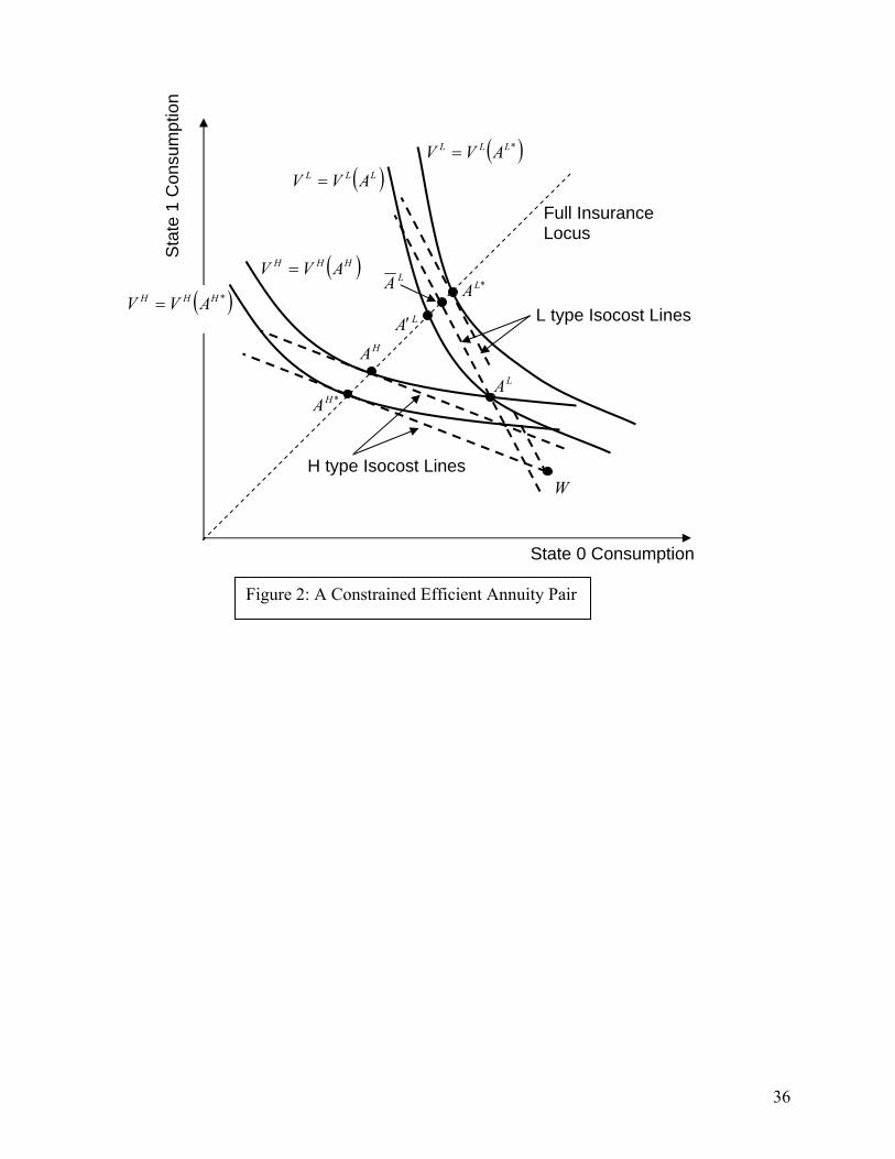
36
LA
State 0 Consumption
Sta
te 1
Con
sum
ptio
n
W
*LA
*HA
( )*LLL AVV = ( )LLL AVV =
( )HHH AVV =
L type Isocost Lines
H type Isocost Lines
HA
( )*HHH AVV =
Figure 2: A Constrained Efficient Annuity Pair
Full Insurance Locus
LA′
LA

37
Figure 3: MWS Equilibrium Annuities if Savings is Impossible (Male population, 3=γ )

38
Figure 4: MWS Equilibrium Annuities if Unobservable Savings is Possible (Male population, 3=γ )
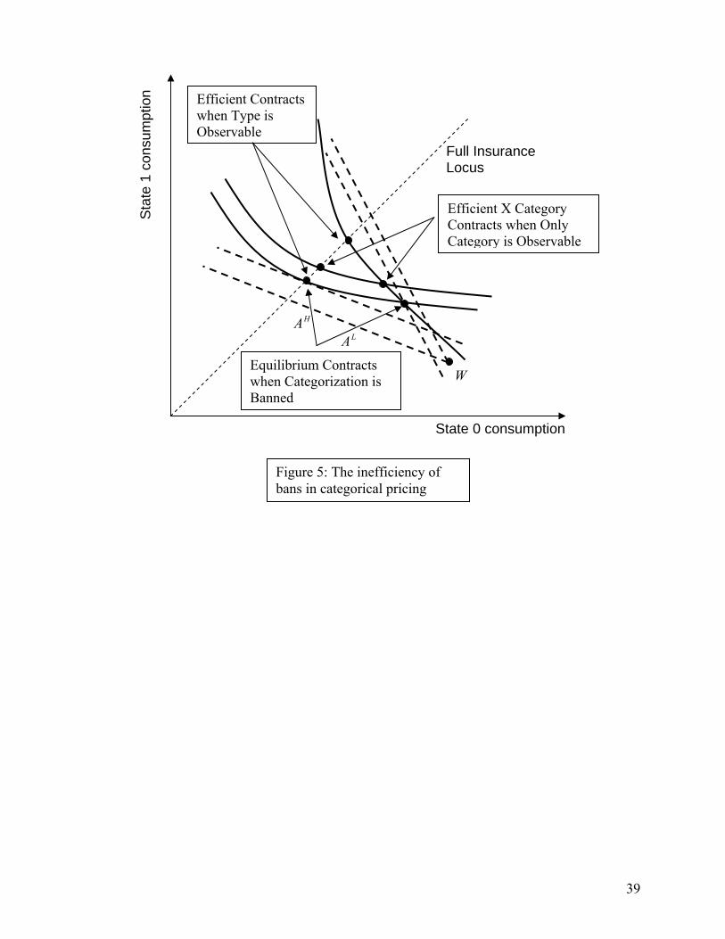
39
State 0 consumption
Sta
te 1
con
sum
ptio
n
W
Full Insurance Locus
Equilibrium Contracts when Categorization is Banned
Efficient Contracts when Type is Observable
Efficient X Category Contracts when Only Category is Observable
HA LA
Figure 5: The inefficiency of bans in categorical pricing
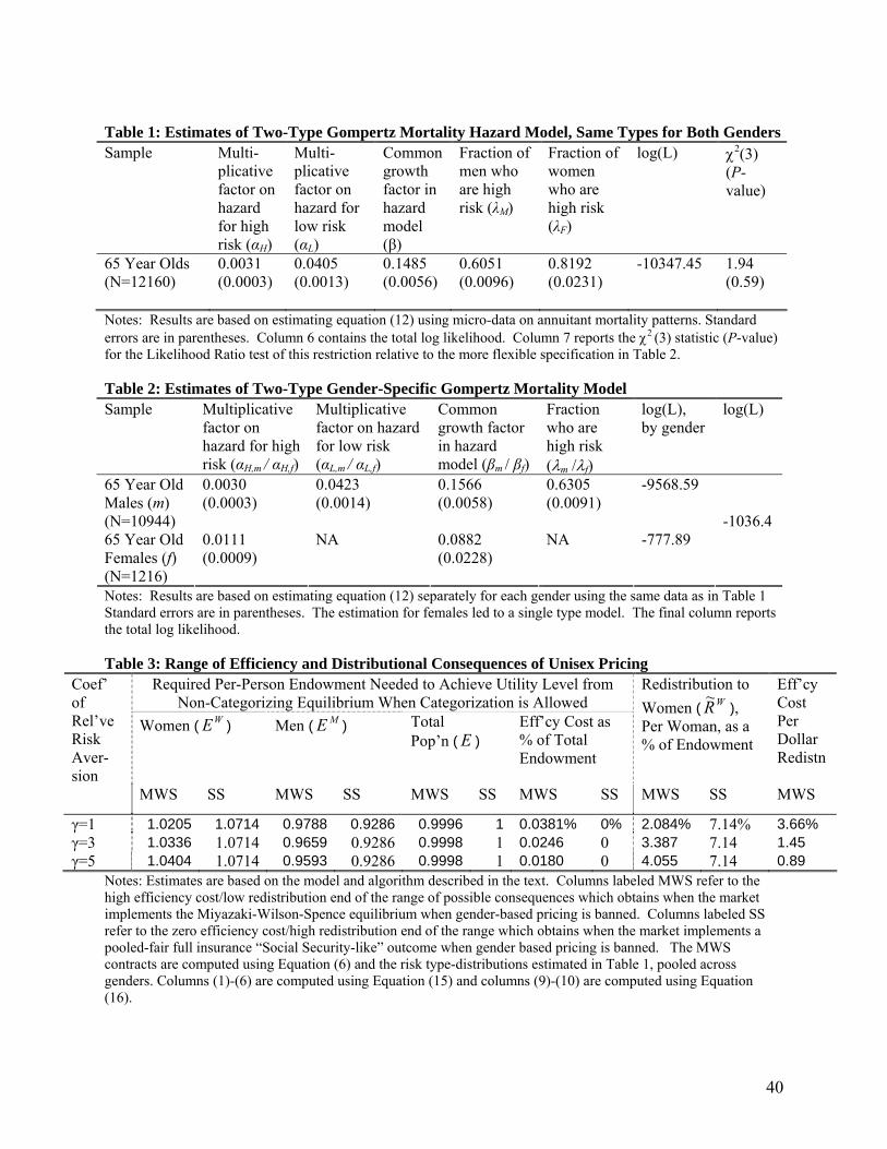
40
Table 1: Estimates of Two-Type Gompertz Mortality Hazard Model, Same Types for Both Genders Sample Multi-
plicative factor on hazard for high risk (αH)
Multi-plicative factor on hazard for low risk (αL)
Common growth factor in hazard model (β)
Fraction of men who are high risk (λM)
Fraction of women who are high risk (λF)
log(L)
χ2(3) (P-value)
65 Year Olds (N=12160)
0.0031 (0.0003)
0.0405 (0.0013)
0.1485 (0.0056)
0.6051 (0.0096)
0.8192 (0.0231)
-10347.45 1.94 (0.59)
Notes: Results are based on estimating equation (12) using micro-data on annuitant mortality patterns. Standard errors are in parentheses. Column 6 contains the total log likelihood. Column 7 reports the χ2
(3) statistic (P-value) for the Likelihood Ratio test of this restriction relative to the more flexible specification in Table 2. Table 2: Estimates of Two-Type Gender-Specific Gompertz Mortality Model Sample Multiplicative
factor on hazard for high risk (αH,m / αH,f)
Multiplicative factor on hazard for low risk (αL,m / αL,f)
Common growth factor in hazard model (βm / βf)
Fraction who are high risk (λm /λf)
log(L), by gender
log(L)
65 Year Old Males (m) (N=10944)
0.0030 (0.0003)
0.0423 (0.0014)
0.1566 (0.0058)
0.6305 (0.0091)
-9568.59
65 Year Old Females (f) (N=1216)
0.0111 (0.0009)
NA
0.0882 (0.0228)
NA -777.89
-1036.4
Notes: Results are based on estimating equation (12) separately for each gender using the same data as in Table 1 Standard errors are in parentheses. The estimation for females led to a single type model. The final column reports the total log likelihood. Table 3: Range of Efficiency and Distributional Consequences of Unisex Pricing
Required Per-Person Endowment Needed to Achieve Utility Level from Non-Categorizing Equilibrium When Categorization is Allowed
Women ( WE )
Men ( ME ) Total Pop’n ( E )
Eff’cy Cost as % of Total Endowment
Redistribution to Women ( WR~ ), Per Woman, as a % of Endowment
Eff’cy Cost Per Dollar Redistn
Coef’ of Rel’ve Risk Aver-sion
MWS SS MWS SS MWS SS MWS SS MWS SS MWS
γ=1 1.0205 1.0714 0.9788 0.9286 0.9996 1 0.0381% 0% 2.084% 7.14% 3.66% γ=3 1.0336 1.0714 0.9659 0.9286 0.9998 1 0.0246 0 3.387 7.14 1.45 γ=5 1.0404 1.0714 0.9593 0.9286 0.9998 1 0.0180 0 4.055 7.14 0.89
Notes: Estimates are based on the model and algorithm described in the text. Columns labeled MWS refer to the high efficiency cost/low redistribution end of the range of possible consequences which obtains when the market implements the Miyazaki-Wilson-Spence equilibrium when gender-based pricing is banned. Columns labeled SS refer to the zero efficiency cost/high redistribution end of the range which obtains when the market implements a pooled-fair full insurance “Social Security-like” outcome when gender based pricing is banned. The MWS contracts are computed using Equation (6) and the risk type-distributions estimated in Table 1, pooled across genders. Columns (1)-(6) are computed using Equation (15) and columns (9)-(10) are computed using Equation (16).
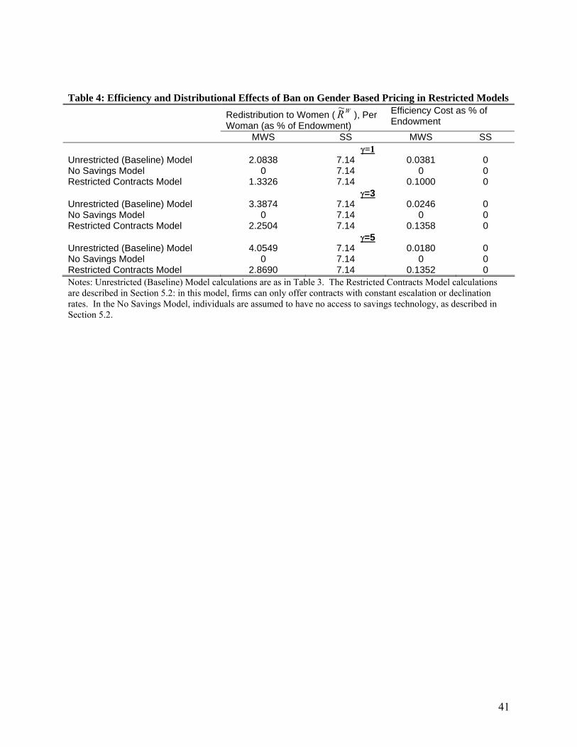
41
Table 4: Efficiency and Distributional Effects of Ban on Gender Based Pricing in Restricted Models Redistribution to Women ( WR~ ), Per
Woman (as % of Endowment) Efficiency Cost as % of Endowment
MWS SS MWS SS γ=1
Unrestricted (Baseline) Model 2.0838 7.14 0.0381 0 No Savings Model 0 7.14 0 0 Restricted Contracts Model 1.3326 7.14 0.1000 0
γ=3 Unrestricted (Baseline) Model 3.3874 7.14 0.0246 0 No Savings Model 0 7.14 0 0 Restricted Contracts Model 2.2504 7.14 0.1358 0
γ=5 Unrestricted (Baseline) Model 4.0549 7.14 0.0180 0 No Savings Model 0 7.14 0 0 Restricted Contracts Model 2.8690 7.14 0.1352 0 Notes: Unrestricted (Baseline) Model calculations are as in Table 3. The Restricted Contracts Model calculations are described in Section 5.2: in this model, firms can only offer contracts with constant escalation or declination rates. In the No Savings Model, individuals are assumed to have no access to savings technology, as described in Section 5.2.

42
Table 5: Sensitivity Analysis for Redistribution and Efficiency Cost Calculations, (γ = 3) Parameter Being Varied and New Value
Redistribution to Women ( WR~ ), Per Woman (as % of Endowment)
Efficiency Cost as % of Endowment
Efficiency Cost Per Dollar of Distribution
MWS SS MWS SS MWS SS
θ (fraction women) 0.1 6.37% 13.63% 0.00% 0% 0.32% 0%0.3 4.84 10.30 0.01 0 0.89 00.5 3.39 7.14 0.02 0 1.45 00.7 2.00 4.17 0.03 0 1.97 00.9 0.66 1.35 0.01 0 2.40 0
Hα , Lα = Mortality hazard at age 65 for low-risk and high-risk type .001, .046 4.72% 8.63% 0.02% 0% 0.91% 0%.002, .043 3.98 7.85 0.02 0 1.18 0
.0031, .041 3.39 7.14 0.02 0 1.45 0.005, .036 2.62 6.01 0.03 0 1.97 0.008, .028 1.65 4.16 0.03 0 3.27 0
( Hα , Lα ),( λm, λf ): Age 65 mortality hazards and type fractions (0.0021,0.2492),(0.6445,0.7798) 4.69% 7.89% 0.01% 0% 0.38% 0%(0.0026,0.0793),(0.6275,0.7968) 3.82 7.45 0.02 0 0.82 0(0.0031,0.0405),(0.6051,0.8192) 3.39 7.14 0.02 0 1.45 0(0.0036,0.0248),(0.5738,0.8505) 3.09 6.92 0.04 0 2.58 0(0.0041,0.0169),(0.5268,0.8976) 2.86 6.78 0.07 0 4.90 0(0.0046,0.0122),(0.4477,0.9770) 2.64 6.62 0.14 0 10.72 0Note: Same calculations as in Table 3 with varying parameters. Results for baseline parameters from Table 3 appear in bold. The mortality hazards for high and low risk types at age 65 are varied while keeping the aggregate mortality rate at age 65 constant. The mortality hazards and type fractions in the bottom panel are varied to keep aggregate type fractions and gender-specific life expectancies constant.

Appendix: Solution Algorithm for Program (7)
This appendix describes and proves the validity of our procedure for solv-ing Program (7) in the text. The difficult part of solving (7) stems from theneed to compute V H(AL), the utility H types achieve when they purchasethe annuity contract designed for the L types and save optimally. We dealwith this difficulty by identifying the structure of the optimal saving patternof deviating H types at the solution to (7).
There are two key features to this structure. First, deviating H types havean incentive to save only at old ages. There is some period n∗ before whichdeviating H types consume the annuity stream. We can therefore solve forV H(AL) by examining the savings behavior in periods n ≥ n∗ only. Second,deviating H types will optimally carry strictly positive wealth forward atevery date n ≥ n∗. Intuitively, absent savings the (IC ′) constraint in (7)could be satisfied with an annuity stream AL which drops off very steeply atvery old ages. Such an annuity would provide H types with an incentive tosave at old ages, undermining the effectiveness and desirability of the steepdrop off. The ability of H types to save therefore pushes the “drop off” inthe annuity AL to earlier dates than would otherwise be optimal. For thisreason, deviating H types never have incentive to borrow at the optimal AL:if they did, AL could be improved by pushing the “drop off” back towardslater ages.
The first feature is important for us: at the heart of our solution procedureis an algorithm to find the n∗ after which the deviating H type’s begin to dosomething other than just consume the annuity stream. The second featureis important because it makes (7) analytically tractable. To see why, contrastthe indirect utility of deviating H types in two situations. In both, take theirbehavior before n to involve the direct consumption of the annuity streamAL prior to n. The two situations only differ in the potential behavior aftern.
In the first situation, we know nothing about the post-n savings behaviorof H types, so we must solve:
V H(A; n) ≡
maxΓ ≡ {c0, · · · , cN} UH(Γ)
subject to(it) ct = at ∀t < n
(iit)∑t
s=n δs (cs − as) ≤ 0 ∀t ≥ n
(17)
43
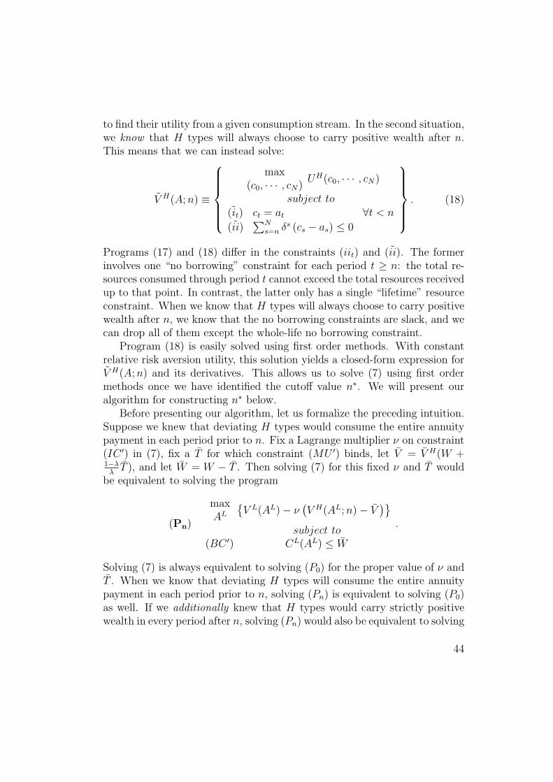
to find their utility from a given consumption stream. In the second situation,we know that H types will always choose to carry positive wealth after n.This means that we can instead solve:
V H(A; n) ≡
max(c0, · · · , cN)
UH(c0, · · · , cN)
subject to
(it) ct = at ∀t < n
(ii)∑N
s=n δs (cs − as) ≤ 0
. (18)
Programs (17) and (18) differ in the constraints (iit) and (ii). The formerinvolves one “no borrowing” constraint for each period t ≥ n: the total re-sources consumed through period t cannot exceed the total resources receivedup to that point. In contrast, the latter only has a single “lifetime” resourceconstraint. When we know that H types will always choose to carry positivewealth after n, we know that the no borrowing constraints are slack, and wecan drop all of them except the whole-life no borrowing constraint.
Program (18) is easily solved using first order methods. With constantrelative risk aversion utility, this solution yields a closed-form expression forV H(A; n) and its derivatives. This allows us to solve (7) using first ordermethods once we have identified the cutoff value n∗. We will present ouralgorithm for constructing n∗ below.
Before presenting our algorithm, let us formalize the preceding intuition.Suppose we knew that deviating H types would consume the entire annuitypayment in each period prior to n. Fix a Lagrange multiplier ν on constraint(IC ′) in (7), fix a T for which constraint (MU ′) binds, let V = V H(W +1−λ
λT ), and let W = W − T . Then solving (7) for this fixed ν and T would
be equivalent to solving the program
(Pn)
maxAL
{V L(AL)− ν
(V H(AL; n)− V
)}
subject to(BC ′) CL(AL) ≤ W
.
Solving (7) is always equivalent to solving (P0) for the proper value of ν andT . When we know that deviating H types will consume the entire annuitypayment in each period prior to n, solving (Pn) is equivalent to solving (P0)as well. If we additionally knew that H types would carry strictly positivewealth in every period after n, solving (Pn) would also be equivalent to solving
44

the program:
(Pn)
maxAL
{V L(AL)− ν
(V H(AL; n)− V
)}
subject to(BC ′) CL(AL) ≤ W
.
When we know the two features of deviating H type’s consumption patternsare satisfied and we know the cutoff n∗, solving (Pn∗) will therefore also solve(7). This is important, because the closed, tractable form of V H(A; n) allowsus to solve (Pn) using first order methods.
We will now present Algorithm 1, which we use to construct n∗. Theremainder of the appendix will be devoted to showing that the solutions to(P0) and (Pn∗) coincide for this n∗. This is formally stated in Proposition 1below, but we will need to establish several lemmas before we can prove it.Once we have proved it, we will know that applying Algorithm 1 to find n∗
and then solving (Pn∗) will solve (7) for the given ν, and we will be done.First we define a parameter n∗max which will play an important role in
Algorithm 1. To motivate it, imagine solving (PN) for AL∗ = (aL∗0 , · · · , aL∗
N ).If it happens that
SHn (aL∗
n )−γ ≥ SHn+1(a
L∗n+1)
−γ for n = 0 · · · , N − 1, (19)
then H types will have no incentive to save when given annuity AL∗. Hence,AL∗ will also solve the tighter program (P0). To see when (19) is possible,consider the first order conditions for aL∗
n and aL∗n+1. These imply
(aL∗n )−γ
(1− ν
SHn
SLn
)≥ (aL∗
n+1)−γ
(1− ν
SHn+1
SLn+1
). (20)
Combining (19) and (20) yields
ν ≤( 1
SHn+1
− 1SH
n
1SL
n+1− 1
SLn
). (21)
Therefore, (19) will only be possible—and AL∗ can only solve (P0)—when ν is
sufficiently low. For higher ν, there will be some t for which ν >
(1
SHn+1
− 1
SHn
1
SLn+1
− 1
SLn
),
45
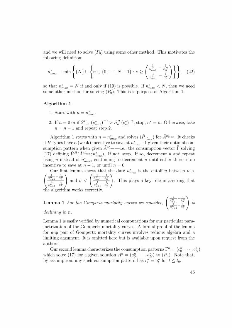
and we will need to solve (P0) using some other method. This motivates thefollowing definition:
n∗max ≡ min
{{N} ∪
{n ∈ {0, · · · , N − 1} : ν ≥
( 1SH
n+1− 1
SHn
1SL
n+1− 1
SLn
)}}, (22)
so that n∗max = N if and only if (19) is possible. If n∗max < N , then we needsome other method for solving (P0). This is is purpose of Algorithm 1.
Algorithm 1
1. Start with n = n∗max.
2. If n = 0 or if SHn−1
(cnn−1
)−γ> SH
n (cnn)−γ, stop, n∗ = n. Otherwise, take
n = n− 1 and repeat step 2.
Algorithm 1 starts with n = n∗max and solves (Pn∗max) for An∗max . It checks
if H types have a (weak) incentive to save at n∗max−1 given their optimal con-sumption pattern when given An∗max—i.e., the consumption vector Γ solving(17) defining V H(An∗max ; n∗max). If not, stop. If so, decrement n and repeatusing n instead of n∗max, continuing to decrement n until either there is noincentive to save at n− 1, or until n = 0.
Our first lemma shows that the date n∗max is the cutoff n between ν >(1
SHn+1
− 1
SHn
1
SLn+1
− 1
SLn
)and ν <
(1
SHn+1
− 1
SHn
1
SLn+1
− 1
SLn
). This plays a key role in assuring that
the algorithm works correctly.
Lemma 1 For the Gompertz mortality curves we consider,
(1
SHn+1
− 1
SHn
1
SLn+1
− 1
SLn
)is
declining in n.
Lemma 1 is easily verified by numerical computations for our particular para-metrization of the Gompertz mortality curves. A formal proof of the lemmafor any pair of Gompertz mortality curves involves tedious algebra and alimiting argument. It is omitted here but is available upon request from theauthors.
Our second lemma characterizes the consumption patterns Γn = (cn0 , · · · , cn
N)which solve (17) for a given solution An = (an
0 , · · · , anN) to (Pn). Note that,
by assumption, any such consumption pattern has cnt = an
t for t ≤ t0.
46
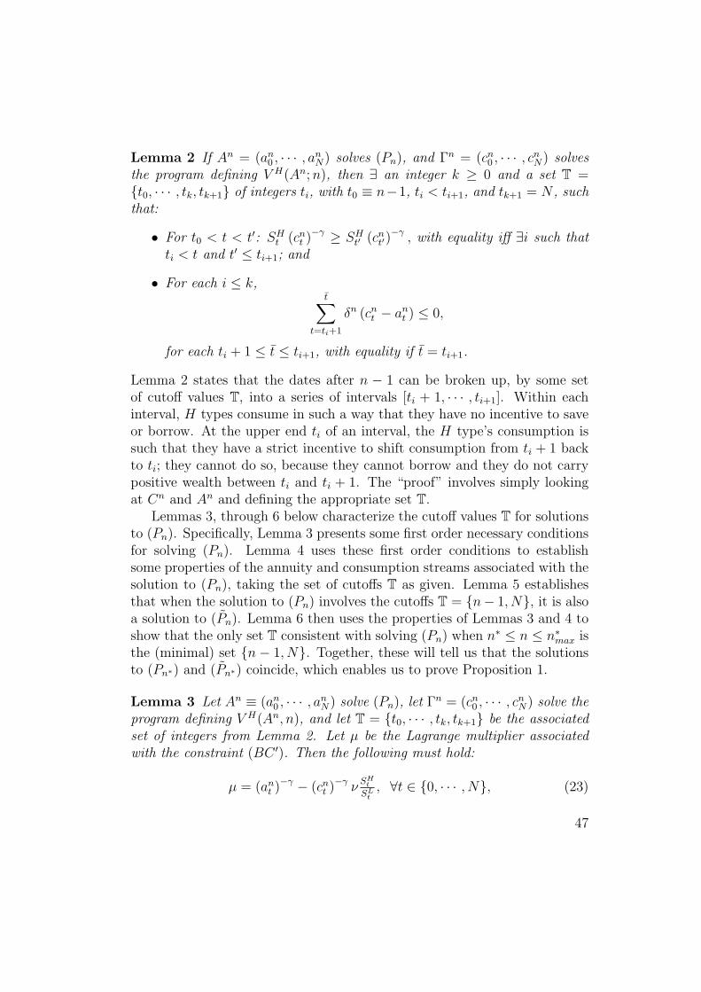
Lemma 2 If An = (an0 , · · · , an
N) solves (Pn), and Γn = (cn0 , · · · , cn
N) solvesthe program defining V H(An; n), then ∃ an integer k ≥ 0 and a set T ={t0, · · · , tk, tk+1} of integers ti, with t0 ≡ n−1, ti < ti+1, and tk+1 = N , suchthat:
• For t0 < t < t′: SHt (cn
t )−γ ≥ SHt′ (cn
t′)−γ , with equality iff ∃i such that
ti < t and t′ ≤ ti+1; and
• For each i ≤ k,t∑
t=ti+1
δn (cnt − an
t ) ≤ 0,
for each ti + 1 ≤ t ≤ ti+1, with equality if t = ti+1.
Lemma 2 states that the dates after n − 1 can be broken up, by some setof cutoff values T, into a series of intervals [ti + 1, · · · , ti+1]. Within eachinterval, H types consume in such a way that they have no incentive to saveor borrow. At the upper end ti of an interval, the H type’s consumption issuch that they have a strict incentive to shift consumption from ti + 1 backto ti; they cannot do so, because they cannot borrow and they do not carrypositive wealth between ti and ti + 1. The “proof” involves simply lookingat Cn and An and defining the appropriate set T.
Lemmas 3, through 6 below characterize the cutoff values T for solutionsto (Pn). Specifically, Lemma 3 presents some first order necessary conditionsfor solving (Pn). Lemma 4 uses these first order conditions to establishsome properties of the annuity and consumption streams associated with thesolution to (Pn), taking the set of cutoffs T as given. Lemma 5 establishesthat when the solution to (Pn) involves the cutoffs T = {n− 1, N}, it is alsoa solution to (Pn). Lemma 6 then uses the properties of Lemmas 3 and 4 toshow that the only set T consistent with solving (Pn) when n∗ ≤ n ≤ n∗max isthe (minimal) set {n− 1, N}. Together, these will tell us that the solutionsto (Pn∗) and (Pn∗) coincide, which enables us to prove Proposition 1.
Lemma 3 Let An ≡ (an0 , · · · , an
N) solve (Pn), let Γn = (cn0 , · · · , cn
N) solve theprogram defining V H(An, n), and let T = {t0, · · · , tk, tk+1} be the associatedset of integers from Lemma 2. Let µ be the Lagrange multiplier associatedwith the constraint (BC ′). Then the following must hold:
µ = (ant )−γ − (cn
t )−γ νSH
t
SLt, ∀t ∈ {0, · · · , N}, (23)
47

ant = cn
t , ∀t < N, (24)
SHt (cn
t )−γ = SHt′ (cn
t′)−γ, ∀t, t′ ∈ {ti + 1, · · · , ti+1} ∀i ∈ {0, · · · , k}, (25)
∑ti+1
t=ti+1 δt(cnt − an
t ) = 0, ∀i ∈ {0, · · · , k}. (26)
Proof. Since ∂V H(An;n)∂an
t= SH
t (cnt )−γ, (23) is the first order necessary con-
dition for ant in (Pn). Conditions (24)-(26) characterize necessary conditions
for Γn to solve the program defining V H(An; n). Condition (24) follows fromthe definition of that program. Both (25) and (26) follow from Lemma 2:(25) states that H type’s consumption is such that they have no incentiveto borrow or save within an interval and (26) states that individuals do notcarry positive wealth from one interval to the next.
By Lemma 3, conditions (23)-(26) are necessary for a solution to (Pn).Lemma 4 shows that for any fixed set of cutoffs T, these four conditions aresatisfied only for a unique annuity and consumption pair. The lemma furtherexamines how this unique pair varies with the Lagrange multiplier µ: sinceµ can be interpreted as a marginal utility of resources and u′(x) = x−γ, the
pair varies with µ as µ−1γ .
Lemma 4 Fix µ > 0 and T. Then there is a unique annuity and con-sumption pair, (a′n0 , · · · , a′nN) ≡ A′n and (c′n0 , · · · , c′nN) = Γ′n, that solves
(23) through (26). Viewed as a function of µ, a′nt (µ) = a′nt (1)µ−1γ and
c′nt (µ) = c′nt (1)µ−1γ .
Proof. Fix a ti. Condition (25) determinesc′ntc′nt′
for any t, t′ in the interval
[ti+1, · · · , ti+1]. (c′nti+1, · · · , c′nti+1) is therefore determined up to a scalar multi-
ple. To pin down this scalar multiple, fix a Wi ∈ R and generate the uniquevector (c′nti+1, · · · , c′nti+1
) consistent with (25) and with Wi =∑ti+1
t=ti+1 δtc′nt .Next, define the function M1 : R→ Rti+1−ti by M1(a
nti+1) ≡ (an
ti+1, · · · , anti+1
),where an
t is defined implicitly via
(ant )−γ − (c′nt )
−γνSH
t
SLt
=(an
ti+1
)−γ − (c′nti+1
)−γνSH
ti+1
SLti+1
,
as required by (23). Similarly, define the function M2 : Rti+1−ti → R viaM2(a
nti+1, · · · , an
ti+1) ≡ ∑ti+1
t=tiδtan
t . Then M2(M1(ati+1)) is strictly increasing
48
in ati+1; hence there is a unique ati+1 such that M2(M1(ati+1)) = Wi. There-
fore, for any Wi, there is a unique pair of vectors(a′nti+1(Wi), · · · , a′nti+1
(Wi))
and(c′nti+1(Wi), · · · , c′nti+1
(Wi))
consistent with
Wi =
ti+1∑t=ti+1
δta′nt (Wi) =
ti+1∑t=ti+1
δtc′nt (Wi)
and with
(a′nt (Wi)
)−γ
−(c′nt (Wi)
)−γ
νSH
t
SLt
=(a′nti+1(Wi)
)−γ
−(c′nti+1(Wi)
)−γ
νSH
ti+1
SLti+1
for all t ∈ {ti + 1, · · · , ti+1}.Clearly, if
{(a′nt (Wi)
)ti+1
t=ti+1,(c′nt (Wi)
)ti+1
t=ti+1
}is the unique pair consis-
tent in this sense with Wi, then
{(βa′nt (Wi)
)ti+1
t=ti+1,(βc′nt (Wi)
)ti+1
t=ti+1
}is
uniquely consistent in this sense with βWi for any β > 0. Via µ, (23) then
pins down a unique Wi and corresponding(a′nti+1(Wi), · · · , a′nti+1
(Wi))
and(c′nti+1(Wi), · · · , c′nti+1
(Wi))
consistent with (23), (25) and (26) for the inter-
val i, and shows that c′nt and a′nt vary with µ as µ−1γ in this interval.
This argument holds for each ti, and hence for each t ≥ n. For t < n, asimilar argument using (24) instead of (25) establishes the same uniquenessresult, completing the proof.
Lemma 4 shows that there is a unique pair An and Γn that satisfies thenecessary conditions for a given fixed T. That is, for any T there is a unique“candidate” for solving (Pn). We will now establish two lemmas about thiscandidate solution. First, Lemma 5 shows that if the candidate associatedwith cutoffs T = {n − 1, N} is indeed a solution to (Pn), then it is also asolution to (Pn). Second, Lemma 6 shows that, when n∗ ≤ n ≤ n∗max, thecandidate for any other T = {n−1, N} cannot solve (Pn) for T = {n−1, N}.Together, they imply that the solution to (Pn∗) solves (Pn∗) as well.
Lemma 5 Consider a solution An to (Pn) and the corresponding Γn solving(17) defining V H(An; n). If the cutoff values T given by Lemma 2 at thissolution are given by T = {n− 1, N}, then An solves (Pn).
49

Proof. When T = {n − 1, N}, Lemma 2 implies that Γn also satisfies thefirst order conditions associated with the program defining V H(An; n), andtherefore solves that program. An is therefore feasible in (Pn). (Pn) is atighter program than (Pn), so An solves (Pn).
Lemma 6 Assume n∗ ≤ n ≤ n∗max. Let A′n = (a′n0 , · · · , a′nN) and Γ′n =(c′n0 , · · · , c′nN) solve (Pn) and the program defining V H(A′n; n), respectively,and let T be the associated cutoffs from Lemma 2. Then T = {n− 1, N}.
Proof. If T 6= {n − 1, N}, take the largest tk ∈ T less than N . For A′n
and Γ′n to solve (Pn) with cutoffs T and the program defining V H(A′n; n),respectively, Lemma 2 requires:
a′ntk ≤ c′ntkand
a′ntk+1 ≥ c′ntk+1.(27)
First suppose, by way of contradiction, that tk ≥ n∗max, where n∗max isdefined in Algorithm 1. Then combining (27) with the necessary condition(23), we observe:
(c′ntk)−γ
(1− ν
SHtk
SLtk
)≤ (c′ntk+1)
−γ
(1− ν
SHtk+1
SLtk+1
). (28)
Lemma 2 also requires:
SHtk
(c′ntk)−γ > SH
tk+1(c′ntk+1)
−γ. (29)
Combining (28) and (29) yields:
SHtk+1
SHtk
(1− ν
SHtk
SLtk
)<
(1− ν
SHtk+1
SLtk+1
)or ν <
1SH
tk+1− 1
SHtk
1SL
tk+1− 1
SLtk
.
This contradicts Lemma 1 when tk ≥ n∗max by Lemma 1.When T = {n− 1, N} at the solution to (Pn), the solutions to (Pn) and
(Pn) coincide by Lemma 5. Having ruled out tk ≥ n∗max, we conclude that(Pn∗max
) is uniquely solved with cutoffs Tn∗max= {n∗max − 1, N} and that the
solutions to (Pn∗max) and (Pn∗max
) coincide.
50

Proceeding by induction, suppose that for some n ≥ n∗, (Pn) is uniquelysolved with cutoffs Tn = {n − 1, N} for each n ≥ n + 1. By Lemma 5, thesolutions to (Pn) and (Pn) must then coincide for n ≥ n + 1. We will provethat Tn = {n − 1, N} by contradiction: suppose there is a solution to (Pn)involving cutoffs T = {n−1, · · · , tk, N} 6= {n−1, N}. From above, tk < n∗max
must hold.Fix µ = 1 (without loss of generality by Lemma 4), and take Γ′n and
A′n as in Lemma 4 for n = n and cutoffs T. Take Γ′′tk+1 and A′′tk+1 as inLemma 4 for n = tk + 1 and cutoffs {tk, N}; then Γ′′tk+1 = Γtk+1 = Γtk+1
and A′′tk+1 = Atk+1 = Atk+1 by the inductive hypothesis. By the argumentin the proof of Lemma 4, c′nt = c′′tk+1
t for t = tk + 1, · · · , N : having fixed µ,there is a unique solution within each interval, and the top intervals for thetwo problems coincide.
By Lemma 2, c′ntk ≥ a′ntk , whereby (23) yields µ ≡ 1 ≥ (a′ntk
)−γ(
1− νSH
tk
SLtk
).
Similarly, since a′′tk+1tk
= c′′tk+1tk
we conclude that 1 =(a′′tk+1
tk
)−γ(
1− νSH
tk
SLtk
).
Therefore, a′′tk+1tk
≤ a′ntk and c′′tk+1tk
≤ c′ntk .To complete the proof, note that if A′n solves (Pn) then Lemma 2 requires
SHtk
(c′ntk)−γ > SH
tk+1(c′ntk+1)
−γ. Since c′′tk+1tk
≤ c′ntk and c′′tk+1tk+1 = c′ntk+1, this implies
SHtk
(c′′tk+1tk
)−γ > SHtk+1(c
′′tk+1tk+1 )−γ. Noting that Γ′′tk+1 = Γtk+1 = Γtk+1, Algo-
rithm 1 implies n∗ ≥ tk + 1, since Algorithm 1 would have stopped at tk + 1,if not before. Since n ≥ n∗ and n ≤ tk, we have reached our contradiction,completing the proof.
We are now ready to state and prove Proposition 1. Proposition 1 statesthat the solution to (Pn∗) solves (P0). This means that (Pn∗) can be usedto solve (7) in the text—all that is additionally required is a search for theproper value of the multiplier ν. Since (Pn) is easily solved, we will be doneonce we have proved Proposition 1.
Proposition 1 If An∗ solves (Pn∗), then An∗ solves (P0) and (Pn∗) where n∗
is the outcome of Algorithm 1.
Proof. A solution An∗ = (an∗0 , · · · , an∗
N ) to (Pn∗) must exist, since theset of A satisfying the constraints is compact and the objective function iscontinuous. Lemmas 4 and 6 together imply that this solution is uniqueand involves the cutoff values T = {n − 1, N}. By Lemma 5, this solutionalso solves (Pn∗). Examination of the first order conditions shows that thissolution to (Pn∗) is unique.
51
Since V H(A; n) ≤ V H(A; 0) for every A, the value of Program (Pn∗)is at least as large as the value of Program (P0). It therefore suffices toshow that V H(An∗ ; n∗) = V H(An∗ ; 0). Let Γn∗ = (cn∗
0 , · · · , cn∗N ) solve the
program defining V H(An∗ ; n∗). Γn∗ must also solve the program (18) definingV H(An∗ ; n∗), or else An∗ couldn’t solve both (Pn) and (Pn). We need onlyto check that Γn∗ also solves the program (17) defining V H(An∗ , 0). Since(17) is a globally concave program and Γn∗ satisfies all of the constraints, it
suffices to show that SHt
(cn∗t
)−γ ≥ SHt+1
(cn∗t+1
)−γfor each t, with equality for
any t at which∑t
s=0 δs(cn∗s − an∗
s ) < 0.
For t ≥ n∗, SHt
(cn∗t
)−γ= SH
t+1
(cn∗t+1
)−γ. This is a necessary condition for
Γn∗ to solve the program defining V H(An∗ ; n∗). If n∗ = 0, we are done.Otherwise, for t < n∗, we have cn∗
t = an∗t , so
∑ts=0 δs(cn∗
s − an∗s ) = 0,
and we need only verify that SHt
(cn∗t
)−γ ≥ SHt+1
(cn∗t+1
)−γ. By Algorithm
1, SHn∗−1
(cn∗n∗−1
)−γ> SH
n∗(cn∗n∗
)−γ. We are therefore done if n∗ = 1.
If n∗ > 1, suppose, by way of contradiction, that
SHt
(cn∗t
)−γ< SH
t+1
(cn∗t+1
)−γ(30)
for some t < n∗ − 1. Since cn∗t = an∗
t for t < n∗,
(an∗
t
)−γ(
1− νSH
t
SLt
)=
(an∗
t+1
)−γ(
1− νSH
t+1
SLt+1
)(31)
by Lemma 3. (30) and (31) can be used to show that ν >
(1
SHt+1
− 1
SHt
1
SLt+1
− 1
SLt
). But
since t < n∗ ≤ n∗max, this is impossible given Algorithm 1 and Lemma 1.
This contradiction shows that SHt
(cn∗t
)−γ ≥ SHt+1 for each t < n∗ − 1, which
completes our proof.
52


