NON-STANDARD SOLUTIONS
TO THE EULER SYSTEM OF
ISENTROPIC GAS DYNAMICS
Dissertation
zur
Erlangung der naturwissenschaftlichen Doktorwurde
(Dr. sc. nat.)
vorgelegt der
Mathematisch-naturwissenschaftlichen Fakultat
der
Universitat Zurich
von
ELISABETTA CHIODAROLI
von
Italien
Promotionskomitee
Prof. Dr. Camillo De Lellis (Vorsitz)
Prof. Dr. Thomas Kappeler
Zurich, 2012


Abstract
This thesis aims at shining some new light on the terra incognita of
multi-dimensional hyperbolic systems of conservation laws by means of
techniques new for the field. Our concern focuses in particular on the
isentropic compressible Euler equations of gas dynamics, the oldest but
yet most prominent paradigm for this class of equations. The theory
of the Cauchy problem for hyperbolic systems of conservation laws in
more than one space dimension is still in its dawning and has been
facing some basic issues so far: do there exist weak solutions for any
initial data? how to prove well-posedness for weak solutions? which is a
good space for a well-posedness theory? are entropy inequalities good
selection criteria for uniqueness? Inspired by these interesting ques-
tions, we obtained some new results here collected. First, we present
a counterexample to the well-posedness of entropy solutions to the
multi-dimensional compressible Euler equations: in our construction
the entropy condition is not sufficient as a selection criteria for unique
solutions. Furthermore, we show that such a non-uniqueness theorem
holds also for a classical Riemann datum in two space dimensions. Our
results and constructions build upon the method of convex integration
developed by De Lellis-Szekelyhidi [DLS09, DLS10] for the incom-
pressible Euler equations and based on a revisited ”h-principle”.
Finally, we prove existence of weak solutions to the Cauchy problem
for the isentropic compressible Euler equations in the particular case
of regular initial density. This result indicates the way towards a more
general existence theorem for generic initial data. The proof ultimately
relies once more on the methods developed by De Lellis and Szekelyhidi
in [DLS09]-[DLS10].
Zusammenfassung
i

In dieser Doktorarbeit studiere ich
Aknowledgements
My first thank goes to my advisor Prof. Dr. Camillo De Lellis for
being a guide and a great font of mathematical inspiration. In him I
found an example of inextinguishable enthusiasm, ideas and taste for
beautiful mathematics. I thank him for all the opportunities he offered
me during my PhD.
I am grateful to my colleagues and friends, who rendered the years
of my PhD a pleasant experience of life and friendship.
My sincere gratitude goes to my family for their continuous support
and encouragement. Finally, I would like to express a special thank to
Lorenzo, my fellow traveller.
Elisabetta Chiodaroli, July 2012.
Contents
Introduction 1
0.1. Hyperbolic systems of conservation laws 2
0.2. Main results and outline of the thesis 9
Chapter 1. The h–principle and convex integration 13
1.1. Partial differential relations and Gromov’s h-principle 14
1.2. The h-principle for isometric embeddings 16
1.3. The h-principle and the equations of fluid dynamics 20
Chapter 2. Non–uniqueness with arbitrary density 33
2.1. Introduction 33
2.2. Weak and admissible solutions to
the isentropic Euler system 35
2.3. Geometrical analysis 40
2.4. A criterion for the existence of infinitely many solutions 46
2.5. Localized oscillating solutions 52
2.6. The improvement step 54
2.7. Construction of suitable initial data 57
2.8. Proof of the main Theorems 62
Chapter 3. Non–standard solutions to the compressible Euler
equations with Riemann data 65
3.1. Introduction 65
3.2. Weak solutions to the incompressible Euler equations with
vortex sheet initial data 66
3.3. The compressible system: main results 70
3.4. Basic definitions 73
3.5. Convex integration 75
3.6. Non–standard solutions with quadratic pressure 77
3.7. Non–standard solutions with specific pressure 89
iii
Chapter 4. Study of a classical Riemann problem for the
compressible Euler equations 103
4.1. Solution of the Riemann problem via wave curves 103
4.2. The Hugoniot locus 107
4.3. Rarefaction waves 108
4.4. Contact discontinuity 109
4.5. Solution of the Riemann problem 109
4.6. The case of general pressure 112
Chapter 5. Existence of weak solutions 117
5.1. Introduction 117
5.2. The problem 118
5.3. Existence of weak solutions 120
Bibliography 125

Introduction
The main topic of this thesis is the study of the compressible Euler
equations of isentropic gas dynamics
(0.1)
∂tρ+ divx(ρv) = 0
∂t(ρv) + divx(ρv ⊗ v) +∇[p(ρ)] = 0
ρ(0, ·) = ρ0
v(0, ·) = v0
whose unknowns are the density ρ and the velocity v of the gas, while
p is the pressure which depends on the density ρ. In particular, we are
concerned with the Cauchy problem (0.1) and with its possible (or not)
well-posedness theory.
The isentropic compressible Euler equations (0.1) are an archetype
for systems of hyperbolic conservation laws. Conservation laws model
situations in which the change of amount of a physical quantity in some
domain is due only to an income or an outcome of that quantity across
the boundary of the domain. Indeed, this is the case also for system
(0.1), where the equations involved state the balance laws for mass and
for linear momentum.
The apparent simplicity of conservation laws, and in particular of
system (0.1), contrasts with the difficulties encountered when solving
the Cauchy problem. To illustrate the mathematical difficulties, let us
say that there has not been so far a satisfactory result concerning the
existence of a solution of the Cauchy problem. The well-posedness the-
ory for hyperbolic conservation laws is presently understood only in the
scalar case (one equation) thanks to seminal work of Kruzkov [Kru70],
and in the one–dimensional case (one space–dimension) via the Glimm
scheme [Gli65] or the more recent vanishing–viscosity method of Bian-
chini and Bressan [BB05]. On the contrary, the general case is very
far from being understood.
For this reason, a wise approach is to tackle some particular examples,
in hope of getting some general insight.
1

2 INTRODUCTION
This motivates our interest on the paradigmatic system of conser-
vation laws (0.1). On the one hand, we can obtain a partial result
on the existence of weak solutions of (0.1) for general initial momenta
and regular initial density, on the other hand, building upon the same
methods (see [DLS09]-[DLS10]), we can prove non–uniqueness for en-
tropy solutions of (0.1) even for Riemann initial data. Our conclusions
provide some answers in the understanding of multi-dimensional hy-
perbolic systems of conservation laws, yet raises and lives open other
ones.
In this introductory chapter, we frame our dissertation presenting
an overview of the theory of hyperbolic systems of conservation laws
and highlighting open problems and challenges of the subject. Finally,
we will present the main results contained in this thesis and we will
outline its structure.
0.1. Hyperbolic systems of conservation laws
Hyperbolic systems of conservation laws are systems of partial dif-
ferential equations of evolutionary type which arise in several problems
of continuum mechanics. One of their characteristics is the appearance
of singularities (known as shock waves) even starting from smooth ini-
tial data. In the last decades a very successful theory has been de-
veloped in one–space dimension but little is known about the general
Cauchy problem in more than one–space dimension after the appear-
ance of singularities. Recently, building on some new advances on the
theory of transport equations, well-posedness for a particular class of
systems has been proved. On the other hand, introducing techniques
which are completely new in this context, it has been possible to estab-
lish an ill-posedness result for bounded entropy solutions of the Euler
system of isentropic gas dynamics (0.1). Connected to these recent
advances, there have been various open questions: how to conjecture
well-posedness for general systems of conservation laws in several space
dimensions? in which functional space? what structural properties of
the Euler system of isentropic gas dynamics underlie the mentioned
ill-posedness result? and in which class of initial data does this result
hold? This thesis was inspired by such challenging questions and at-
tempted to move some steps forward in the process of answering them.
0.1. HYPERBOLIC SYSTEMS OF CONSERVATION LAWS 3
0.1.1. Survey on the classical theory. The theory of nonlinear
hyperbolic systems of conservation laws traces its origins to the mid
19th century and has developed over the years conjointly with contin-
uum physics. The great number of books on the theoretical and nu-
merical analysis published in recent years is an evidence of the vitality
of the field. But, what does the denomination “hyperbolic systems of
conservation laws” encode? They are systems of nonlinear, divergence
structure first-order partial differential equations of evolutionary type,
which are typically meant to model balance laws. In fact, the vast ma-
jority of noteworthy hyperbolic systems of conservation laws came up in
physics, where differential equations were derived from corresponding
statements of balance of an extensive physical quantity coupled with
constitutive relations for a material body (see for instance [Daf00]).
In the most general framework, the field equation resulting from this
coupling process reads as
(0.1) ∂tU + div[F (U)] = 0
where the unknown is a vector valued function
(0.2) U = U(t, x) = (U1(t, x), ..., Uk(t, x)) ((t, x) ∈ Ω ⊂ Rt × Rmx ),
the components of which are the densities of some conserved variables
in the physical system under investigation, while the flux function F
controls the rate of loss or increase of U through the spatial boundary
and satisfies suitable “hyperbolicity conditions”, namely that for every
fixed U and ν ∈ Sm−1, the k × k matrix
m∑α=1
ναDFα(U)
has real eigenvalues and k linearly independent eigenvectors.
Solutions to hyperbolic conservation laws may be visualized as prop-
agating waves. When the system is nonlinear, the profile of compres-
sion waves gets progressively steeper and eventually breaks, generating
jump discontinuites which propagate on as shocks. This behavior is
demonstrated by the simplest example of a nonlinear hyperbolic con-
servation law in one space variable, namely the Burgers equation
(0.3) ∂tU(t, x) + ∂x
(1
2U2(t, x)
)= 0.

4 INTRODUCTION
The appearance of singularities, even when starting from regular initial
data, drives the theory to deal with weak solutions. This difficulty is
compounded further by the fact that, in the context of weak solutions,
uniqueness is lost. To see this, one can consider the Cauchy problem
for the Burgers equation (0.3), with initial data
(0.4) u(0, x) =
− 1, x < 0
1, x > 0.
The problem (0.3), (0.4) admits infinitely many solutions, including
the family
uβ(t, x) =
− 1, −∞ < x ≤ −txt, −t < x ≤ −βt
− β, −βt < x ≤ 0
β, 0 < x ≤ βtxt, βt < x ≤ t
1, x > 0,
for any β ∈ [0, 1].
It thus becomes necessary to devise proper criteria for weeding out
unstable, physically irrelevant, or otherwise undesirable solutions, in
hope of singling out admissible weak solutions. The issue of admissi-
bility of weak solutions to hyberbolic systems of conservation laws is
a central question of the theory and stirred up a debate quite early
in the development of the subject. Continuum physics naturally in-
duces such admissibility criteria through the Second Law of Thermo-
dynamics. These may be incorporated in the analytical theory, either
directly, by stipulating outright that admissible solutions should satisfy
“entropy” inequalities, or indirectly, by equipping the system with a
minute amount of diffusion, which has negligible effect on smooth solu-
tions but reacts stiffly in the presence of shocks, weeding out those that
are not thermodynamically admissible. In the framework of the general
theory of hyperbolic systems of conservation laws, the use of entropy
inequalities to characterize admissible solutions was first proposed by
Kruzkov [Kru70] and then elaborated by Lax [Lax71]. The idea of
regarding inviscid gases as viscous gases with vanishingly small viscos-
ity is quite old; there are hints even in the seminal paper by Stokes
[Sto48]. The important contributions of Rankine [Ran70], Hugoniot
[Hug89] and Rayleigh [Ray10] helped to clarify the issue.

0.1. HYPERBOLIC SYSTEMS OF CONSERVATION LAWS 5
From the standpoint of analysis, a very elegant, definitive theory
is available for the case of scalar conservation laws, in one or several
space dimensions. The special feature that sets the scalar balance law
apart from systems of more than one equation is the size of its family
of entropies: in the scalar case the abundance of entropies induces an
effective characterization of admissible weak solutions as well as very
strong L1-stability and L∞-monotonicity properties. Armed with such
powerful a priori estimates, one can construct admissible solutions in
a number of ways. In the one-dimensional case the qualitative theory
was first developed in the 1950’s by the Russian school, headed by
Oleinik [Ole54, O.A57, O.A59], while the first existence proof in
several space dimensions was established a few years later by Conway
and Smoller [CS96], who recognized the relevance of the space BV .
The definitive treatment in the space BV was later given by Volpert
[Vol67]; building on Volpert’s work, Kruzkov [Kru70] proved the well-
posedness for admissible weak solutions. As a consequence of Kruzkov’s
results when the initial data are functions of locally bounded variation
then so are the solutions. Remarkably, even solutions that are merely
in L∞ exhibit the same geometric structure as BV functions, with
jump discontinuities assembling on “manifolds” of codimension one (see
[DLOW03], [DLR03] and [DLG05])
By contrast, when dealing with systems of conservation laws, it is
still a challenging mathematical problem to develop a theory of well-
posedness for the Cauchy problem of (0.1) which includes the formation
and evolution of shock waves. In one space dimension, namely when
m = 1 in (0.2), this problem has found recently a quite satisfactory and
general answer, thanks to the efforts of generations of mathematicians:
the general mathematical framework of the theory was set in the se-
minal paper of Lax [Lax57]; the first existence result is due to Glimm
[Gli65] in the sixties; Bianchini and Bressan [BB05] finally proved
a well-posedness result. Glimm’s scheme gives the sole result of any
generality concerning Cauchy problems and makes use of functions of
bounded total variation on R. The higher dimensional case is terra
incognita: how to conjecture stability is still an open problem. Indeed,
in several space dimensions, the situation is clearly less favourable: the
success of the spaces L∞ and BV in one–dimensional space is due to the
fact they are algebras allowing for the treatment of the rather strong
non–linearity of the equations; however, the works of Brenner [Bre66]

6 INTRODUCTION
and Rauch [Rau86], which are concerned with linear systems, show
that these spaces cannot be adapted to the multi–dimensional case.
We are thus in presence of a paradox which has up to the present not
been resolved: to find a function space which is an algebra, probably
constructed on L2 and which contains enough discontinuous solutions.
Moreover, even a general existence result for weak solutions in more
than one space dimension is missing so far. The theory is in its infancy.
0.1.2. Recent results. Recently, some attention was devoted to
a first “toy example” falling in the class (0.1). This system, called
Keyfitz–Kranzer system, is clearly very peculiar and, compared to the
most relevant systems coming from the physical literature, has many
more features. It reads as
(0.5)
∂tu+
∑mj=1
∂∂xj
(f j(|u|)u) = 0
u(0, ·) = u0
where for any j = 1, . . . ,m the map f j : R+ → R is assumed to be
smooth. In this case the non–linearity depends only on the modulus of
the solutions. Most notably the system (0.5) decouples into a nonlinear
conservation law for the modulus of ρ := |u|
∂tρ+ div(f(ρ)ρ) = 0
and a system of linear transport equations for the angular part θ :=
u/ |u|∂tθ + f(ρ)−∇θ = 0.
However, it does develop singularities in finite time and a theory of
well–posedness of singular solutions was still lacking up to few years
ago. Thanks to a groundbreaking paper of Ambrosio (see [Amb04]),
it was possible to solve this problem in a very general and satisfactory
way (see [ADL03]): well posedness of renormalized entropy solutions
in the class of maps u ∈ L∞([0, T ]×Rm;Rk) with |u| inBVloc has been
proven by Ambrosio, Bouchut and De Lellis in [ABDL04]. Moreover,
the problem has been used to show that, even in this very particular
case, there is no hope of getting estimates in some of the classical
function spaces which are used in the one-dimensional theory.
In a recent work De Lellis and Szekelyhidi found striking counterex-
amples to the well-posedness of bounded entropy solutions to the isen-
tropic system of gas-dynamics (0.1) (see [DLS10]). These examples

0.1. HYPERBOLIC SYSTEMS OF CONSERVATION LAWS 7
build on a previous work ([DLS09]) where they introduced techniques
from the theory of differential inclusions to construct very irregular so-
lutions to the incompressible Euler equations. The isentropic system
of gas dynamics in Eulerian coordinates (0.1) is the oldest hyperbolic
system of conservation laws. The hyperbolicity condition for system
(0.1) reduces to the monotonicity of the pressure as a function of the
density: p′(ρ) > 0. In this thesis the pressure p will always satisfy
this assumption. Weak solutions of (0.1) are bounded functions which
solve the system in the sense of distributions. Admissible (or entropy)
solutions can be characterized as those weak solutions which satisfy an
additional inequality, coming from the conservation law for the energy
of the system. In the paper [DLS10], De Lellis and Szekelyhidi show
L∞ initial data, with strictly positive piecewise constant density, which
allow for infinitely many admissible solutions of (0.1) in more than one
space dimension, all with strictly positive density:
Theorem 0.1.1 (Theorem from [DLS10]). Let n ≥ 2. Then, for
any given function p, there exist bounded initial data (ρ0, v0) with ρ0 ≥c > 0 for which there are infinitely many bounded admissible solutions
(ρ, v) of (0.1) with ρ ≥ c > 0.
This result proves that the space L∞ is ill-suited for well-posedness
of entropy solutions; moreover it makes us believe that admissibility
inequalities are not the “right” selection criteria. Of course, from The-
orem 0.1.1 arises a cascade of questions which point in many grey areas;
some of these open questions are at the core of this dissertation.
0.1.3. Motivating problems. In this paragraph, we summarize
the main issues which motivated the research presented in this thesis.
They do not exhaust the immeasurable amount of open problems in the
field of hyperbolic systems of conservation laws but they are indicative
of the topicality of this branch of mathematics. Moreover, as illustrated
by the following motivating questions, our concern is not only for the
novelty of the results such questions could lead to, but also for the
techniques involved.
• Existence results : the lack of satisfactory existence results for
weak solution of multi–dimensional systems of conservation
laws is a glaring symptom of the difficulties underlying the
theory. In particular, for bounded initial data, but of arbi-
trary size, only 2 × 2 systems in one–space dimension have

8 INTRODUCTION
been tackled by the method of compensated compactness. Is it
possible to prove some existence result at least for the partic-
ular system of isentropic gas dynamics?
• Well-posedness of admissible solutions : how to separate the
wheat from the chaff, the solutions observed in nature (the
physically admissible ones) from those that are only mathe-
matical artefacts is one of the central questions in the theory
of multi–dimensional systems of conservation laws. In particu-
lar, are entropy (admissibility) inequalities efficient as selection
criteria? Theorem 0.1.1 seems to give a negative answer to the
aforemethioned question. Should this inefficiency of entropy
inequalities believed to be a “universal law”?
• Ill-posedness for the isentropic Euler system: the surprising
result 0.1.1 from [DLS10] left unsolved the question whether
the system (0.1) directly allows for the construction of the
paper [DLS10]. Such a issue is connected not only to the
efficiency of admissible criteria to wheed out non–physical so-
lutions, but also to a development of the techniques on which
[DLS10] bases.
• Ill-initial data: relying only on [DLS10] one could argue that
phenomena of ill-posedness could be restricted to very partic-
ular initial data and that for a large class of them, one could
hope for a uniqueness theorem. We aimed at understanding
better for which initial data such constructions are possible.
In particular we questioned the case of Riemann initial data.
• Further applications : the new method introduced in [DLS09]
has been extended in a quite direct way to the isentropic sys-
tem of gas-dynamics. Another interesting question concerns
possible extensions and further applications of the idea com-
ing from [DLS10]; for instance could it be applied to other
systems of conservation laws?
• Suitable functional spaces : The inadeguacy of the spaces L∞ or
BV for multi–dimensional systems of conservation laws raises

0.2. MAIN RESULTS AND OUTLINE OF THE THESIS 9
the issue of finding another functional space for the study of
weak solutions. But no satisfactory space has been suggested
until now.
0.2. Main results and outline of the thesis
This thesis consists of five chapters whose content we are going to
disclose.
The results here presented represent new developments and applica-
tions of the innovative approach introduced by De Lellis and Szekelyhidi
in [DLS09]-[DLS11]. Their methods brought in the realm of fluid dy-
namics techniques coming from Gromov’s convex integration [Gro86]
and strategies from the theory for differential inclusions [KMS03] and
remarkably combined these tools to construct non-standard solutions
to the incompressible Euler equations and to the compressible ones as
well. Since our achievements strongly rely on this new approach, we
devote Chapter 1 to a brief compendium on the related background
theory. In Chapter 1 we aim at introducing the reader to the interest-
ing theory lying behind Theorem 0.1.1. In particular, we will explain
how Gromov’s work on partial differential relations and on convex in-
tegration together with Kirchheim, Muller and Sverak’s approach to
study the properties of nonlinear partial differential equations can con-
cur to construct solutions to equations from fluid dynamics. We will
also hint the analogies between problems in differential geometry, where
the idea of convex integration originally arose, and the incompressible
Euler equations. Finally, we will give an overview of the recent results
in fluid dynamics obtained as further advancements of De Lellis and
Szekelyhidi’s ideas.
The Introduction together with the first chapter provides a pref-
ace to the core of the thesis: indeed, in the subsequent chapters, the
tools introduced in Chapter 1 will be applied to the compressible Euler
equations (0.1) allowing for new results.
Chapter 2 contains the first important theorem of the thesis:
Theorem 0.2.1 (Non-uniqueness of entropy solutions with arbi-
trary density). Let n ≥ 2. Then, for every periodic ρ0 ∈ C1 with
ρ0 ≥ c > 0 and for any given function p, there exist an initial ve-
locity v0 ∈ L∞ and a time T > 0 such that there are infinitely many

10 INTRODUCTION
bounded admissible solutions (ρ, v) of (0.1) on Rn × [0, T [, all with
density bounded away from 0.
This theorem is an improvement of Theorem 0.1.1: using the same
techniques as in Theorem 0.1.1, we can show that the same non-
uniqueness result holds for any choice of the initial density (see also
[Chi11]). This highlights that the main role in the loss of unique-
ness is due to the velocity field. While the proof of Theorem 0.1.1 re-
lies on a non-uniqueness result for the incompressible Euler equations,
and hence yields “piecewise incompressible” solutions, Theorem 0.2.1
is achieved by applying directly to (0.1) De Lellis and Szekelyhidi’s
ideas. Yet, the solutions constructed in Theorem 0.2.1 allow for wild
oscillations only in the velocity. The general case which would include
wild oscillations in the density as well is presently under investigation
(cf. [CDLK]).
The initial data v0 in Theorem 0.2.1 are ad hoc constructed and
in principle could be very irregular. A surprising corollary of De Lellis
and Szekelyhidi’s result on the incompressible Euler equations is that
a classical Riemann datum follows in the class of initial data allowing
for very wild solutions:
Theorem 0.2.2 (Non-standard solutions of a Riemann problem).
For certain choices of the pressure law p with p′ > 0 and for some
specific Riemann initial data there exist infinitely many bounded en-
tropy solutions of the compressible Euler equations (0.1) in two space
dimensions, all with density bounded away from 0.
The proof of Theorem 0.2.2 is the content of Chapter 3. Theo-
rem 0.2.2 entails that the classical entropy inequality does not ensure
uniqueness of the solutions even for this very natural initial condition.
Though the solutions of Theorem 0.2.2 are very irregular, it is rather
unclear which could be a good space for well-posedness. Let us note
that among the pressure laws for which Theorem 0.2.2 holds, there
is the physically relevant pressure p(ρ) = ρ2. Indeed the quadratic
pressure is predicted from classical kinetic theory in two space dimen-
sions. The inspiration for such a result came from a recent paper by
Szekelyhidi [Sz1], where the vortex sheet initial datum for the incom-
pressible Euler system is investigated. In Chapter 3 we also present
an alternative proof of Szekelyhidi’s result. However, the different role

0.2. MAIN RESULTS AND OUTLINE OF THE THESIS 11
of the pressure term in the compressible Euler system with respect to
the incompressible one requires new ideas and constructions involved
in the proof of Theorem 0.2.2.
In Chapter 4 we restrict our attention to the 1-dimensional Rie-
mann problem for the compressible Euler equations with the same
choice of initial data allowing for Theorem 0.2.2 (which indeed de-
pend only on one space variable): we show that such a problem admits
unique self-similar solutions (even with the same choice of pressure law
as in Theorem 0.2.2). The uniqueness of self–similar solutions is proven
by direct construction of the admissible wave fun. Theorem 0.2.2 shows
that as soon as the self–similarity assumption runs out, uniqueness is
lost.
Chapter 5 is devoted to the last main result of the thesis:
Theorem 0.2.3 (Existence of weak solution with arbitrary momen-
tum). Let ρ0 ∈ C1 and v0 ∈ L2. Then there exists a weak solution (ρ, v)
(in fact, infinitely many) of the Cauchy problem for the compressible
Euler equations (0.1) with intial data (ρ0,m0).
Theorem 0.2.3 is just a first step towards the most desirable result
of existence of weak solutions of (0.1) starting out from any given
bounded initial density and momentum. Such an outcome would be
of great impact, since so far no existence result for weak solutions of
multi-dimensional hyperbolic systems of conservation laws with generic
initial data is available. Of course Theorem 0.2.3 is able to deal only
with regular initial densities, but the more general result is believed to
hold building on the improvement of Theorem 0.2.1 (see [CDLK]).
The thesis is conceived in such a way that every chapter can be
read both as the continuation of what precedes or independently.


CHAPTER 1
The h–principle and convex integration
The h-principle is an umbrella–concept forged by Gromov in 1969
([Gro86]) to unify a series of counterintuitive results in topology and
differential geometry. This principle is a strong property characterizing
the set of solutions of differential relations : a differential relation is soft
or abides by the h-principle if its solvability can be determined on the
basis of purely homotopic calculus. By differential relation we mean
a constraint on maps between two manifolds and on their derivatives
as well. PDEs are examples of differential relations. It is striking that
many differential relations, mostly rooted in differential geometry and
topology, are soft. Two famous examples of the softness phenomenon
are the Nash-Kuiper C1 isometric embedding theory and the Smale’s
sphere eversion.
Why are we interested in the h–principle? It is surprising how the
results on the isentropic Euler equations of gas dynamics presented in
this thesis are based on a revisited h-principle. This new variant of
h-principle has been first devised by De Lellis and Szekelyhidi for the
incompressible Euler equations (see [DLS09]) and lead to new develop-
ments for several equations in fluid dynamics as the ones of this thesis.
Indeed, even if the original h-principle of Gromov pertains to various
problems in differential geometry, De Lellis and Szekelyhidi showed in
their groundbreaking paper [DLS09] that the same principle and sim-
ilar methods could be applied to problems in mathematical physics.
The work by De Lellis and Szekelyhidi found its breeding ground in
the important paper by Muller and Sverak [MS03], where they ex-
tended the method of convex integration (introduced by Gromov to
prove the h-principle) to Lipschitz mappings and noticed the strong
connections between the existence theory for differential inclusions and
the h-principle.
We do not pretend here to give an account of the extremely wide
literature on this topic, but we rather prefer to illustrate some specific
13

14 1. THE H –PRINCIPLE AND CONVEX INTEGRATION
instances of the h-principle as a jumping off point for a general un-
derstanding of the subject. In particular, we will spend some words
on the method of convex integration which will be recalled in the next
chapters for the arguments of our constructions.
1.1. Partial differential relations and Gromov’s h-principle
In this section we will introduce the idea behind the h-principle by
illustrating Gromov’s original formalism.
A partial differential relation R is any condition imposed on the par-
tial derivatives of an unknwon function. A solution ofR is any function
which satisfies this relation. Any differential relation has an underly-
ing algebraic relation which one gets by substituting derivatives by
new independent variables. A simple example of differential relations
are ordinary differential equations or inequalities. We can consider,
for instance, the differential equation y′(x) = y2(x); then the under-
lying algebraic relation is obtained by introducing the new variable z
in place of the derivative y′: the resulting relation is simply z = y2
seen as a constraint in R3 with coordinates (x, y, z). In this language,
a solution of the corresponding algebraic relation is called a formal so-
lution of the original differential relation R. The difference between
genuine and formal solutions in this specific example becomes clear as
soon as we interpret genuine solutions as functions (in fact sections)
f : R → R3, f(x) = (x, y(x), y′(x)) with y′(x) = y2(x) (this amounts
to using the language of jets which we do not want to get into herein).
Clearly, the existence of a formal solution is a necessary condition for
the solvability of a differential relation R. In the previous example,
formal solutions are functions g : R → R3, g(x) = (x, y(x), z(x)) with
z(x) = y2(x). The philosophy behind the h-principle consists in the
following: before trying to solve R one should check whether R admits
a formal solution. The problem of finding formal solutions is of purely
homotopy-theoretical nature. It could seem, at first thought, that exis-
tence of a formal solution cannot be sufficient for the genuine solvability
of R. Indeed, finding a formal solution is an algebraic problem which
is a dramatical simplification of the original differential problem. Thus
it came as a big surprise when it was discovered in the second half
of the twentieth cetury that there exist large and geometrically inter-
esting classes of differential relations for which the solvability of the
formal problem is sufficient for genuine solvability. Moreover, for many

1.1. PARTIAL DIFFERENTIAL RELATIONS AND GROMOV’S H -PRINCIPLE15
of these relations the spaces of formal and genuine solutions turned out
to be much more closely related than one could expect. This property
was formalized by Gromov [Gro86] as the following:
• Homotopy principle (h-principle). A differential relation
R satisfies the h-principle, or the h-principle holds for solutions
of R, if every formal solution of R is homotopic to a genuine
solution of R through a homotopy of formal solutions.
The term “h-principle” was introduced and popularized by M. Gro-
mov in his book [Gro86]. It is now clear that the h-principle does not
hold for the differential equation y′(x) = y2(x) (we consider global so-
lutions), while we could prove the h-principle for the equation y′(x) =
y(x) since every formal solution f(x) = (x, y(x), y(x)) can be joined
via a homotopy Ht of formal solutions to the genuine solution h(x) =
(x, exp(x), exp(x)) simply choosing Ht(x) = (1− t)f(x) + th(x). These
examples are of course trivial and not typical of situations where the
h-principle is useful. In fact, the h-principle is rather useless in the
classical theory of (ordinary or partial) differential equations because
there it fails or holds for some trivial, or at least well known reasons,
as in the above examples.
By contrast, for many differential relations rooted in topology and
geometry the notion of h-principle appeared to be fundamental. There
are several amazing unexpected cases in which the h-priciples holds. A
particular problem which abydes by the h-principle can also be called
soft. As already mentioned, the softness phenomena was first discov-
ered in the fifties by Nash [Nas54] for isometric C1-immersions and
by Smale [Sma58] for differential immersions. However, instances of
the soft problems appeared earlier. In his dissertation and later in his
book [Gro86], Gromov transformed Smale’s and Nash’s ideas into two
powerful methods for solving partial differential relations: continuous
sheaves method and the convex integration method. In the next sec-
tion we will give an overview on Nash’s contruction, where the “spirit”
of convex integration originally arose.
In the language pertainig to Gromov, the idea lying behind con-
vex integration can be illustrated through an easy example which is
suggested in [EM02]. Let us call a path
r : I = [0, 1]→ R2, r(t) := (x(t), y(t)),

16 1. THE H –PRINCIPLE AND CONVEX INTEGRATION
short if x′(t)2 + y′(t)2 < 1 a.e. t ∈ I. The inequality defining a short
path is nothing else that a particular instance of partial differential
relation. It easy to prove that any short path can be C0-approximated
by a solution of the equation x′(t)2 + y′(t)2 = 1 a.e. t ∈ I, which is
another differential relation. This implies that the space of solutions
I → R2 of the differential equation x′(t)2 + y′(t)2 = 1 is C0-dense in
the space of solutions of the differential inequality x′(t)2 + y′(t)2 < 1.
This elementary example illuminates the following idea at the core of
convex integration: given a first order differential relation for maps
I → Rq, it is useful to consider a “relaxed” differential relation which
is the pointwise convex hull of the original relation
1.2. The h-principle for isometric embeddings
1.2.1. Isometric embedding problem. Let Mn be a smooth
compact manifold of dimension n ≥ 2, equipped with a Riemann-
ian metric g. An isometric immersion of (Mn, g) into Rm is a map
u ∈ C1(Mn;Rm) such that the induced metric agrees with g. In local
coordinates this amounts to the system
(1.1) ∂iu · ∂ju = gij
consisting of n(n + 1)/2 equations in m unknowns. If in addition u
is injective, it is an isometric embedding. Analougously, one defines a
short embedding as a map u : Mn → Rm such that the metric induced
on M by u is shorter than g. In coordinates this translates into (∂iu ·∂ju) ≤ (gij) in the sense of quadratic forms. Geometrically being short
means that the embedding shrinks the length of curves. Equally, being
isometric means that the length of curves is preserved.
The well-known result of Nash and Kuiper says that any short em-
bedding in codimension one can be uniformly approximated by C1
isometric embeddings.
Theorem 1.2.1 (Nash-Kuiper theorem). If m ≥ n + 1, then any
short embedding can be uniformely approximated by isometric embed-
dings of class C1.
Note that Theorem 1.2.1 is not merely an existence theorem, but it
shows that there exists a huge (essentially C0-dense) set of solutions.
Such a density of solutions is reminiscent of the example on short paths
presented in the previous section. This type of abundance of solutions

1.2. THE H -PRINCIPLE FOR ISOMETRIC EMBEDDINGS 17
is a central aspect of Gromov’s h-principle, for which the isometric em-
bedding problem is a primary example. Indeed, we could ask whether
there exists a regular homotopy ft : S2 → R3 which begins with the
inclusion f0 of the unit sphere and ends with an isometric immersion f1
into the ball of radius 1/2. One of the many counterintuitive implica-
tions of Nash and Kuiper’s theorem is that we can answer positively to
this question in case of C1-immersions: S2 can be C1 isometrically em-
bedded into an arbitrarily small ε-ball in Euclidean 3-space (for small
ε there is no such C2). The h-principle for isometric embeddings is
rather striking, especially when compared to the classical rigidity re-
sult concerning the Weyl problem: if (S2, g) is a compact Riemannian
surface with positive Gauss curvature and u ∈ C2 is an isometric im-
mersion into R3, then u is uniquely determined up to a rigid motion.
Thus it is clear that isometric immersions have a completely different
qualitative behaviour at low and high regularity (i.e. below and above
C2).
The proof of Theorem 1.2.1 involves an iteration technique called
convex integration.
1.2.2. Nash-Kuiper’s general scheme. The general scheme of
the construction upon which the main results of this thesis build are
strongly inspired by the method of Nash and Kuiper. It is then in-
teresting to sketch here the Nash-Kuiper scheme. For simplicity we
assume g to be smooth. Let us set some notation: given an immersion
u : Mn → Rm, we denote by u]e the pullback of the standard Euclidean
metric e through u, so that in local coordinates
(u]e)ij = ∂iu · ∂ju.
Moreover we define
n∗ =n(n+ 1)
2.
A Riemannian metric g on Rn is said to be primitive if g = α(x)(dl)2,
where l = l(x) is a linear function on Rn and α is a non-negative
function with compact support. A Riemannian metric g on a manifold
M is called primitive if there exists a local parametrization φ : Rn →U ⊂M such that supp g ⊂ U and φ]g is a primitive metric on Rn.
For the sake of clarity, we will give the ideas for the proof of the
following simplified version of Theorem 1.2.1
18 1. THE H –PRINCIPLE AND CONVEX INTEGRATION
Theorem 1.2.2. Let Ω be an open bounded subset of Rn equipped
with the Riemannian metric g and let u be a smooth strictly short
immersion of (Ω, g) into (Rm, e), with m ≥ n + 2. Then, for every
ε > 0 there exists a C1 isometric immersion u : Ω → Rm such that
‖u− u‖C0(Ω) < ε, i.e.
• u ∈ C1(Ω);
• ∂iu · ∂ju = gij in Ω;
• ‖u− u‖C0(Ω) < ε.
The proof of Theorem 1.2.2 is based on an iteration of stages, and
each stage consists of several steps whose purpose we are going to
unravel.
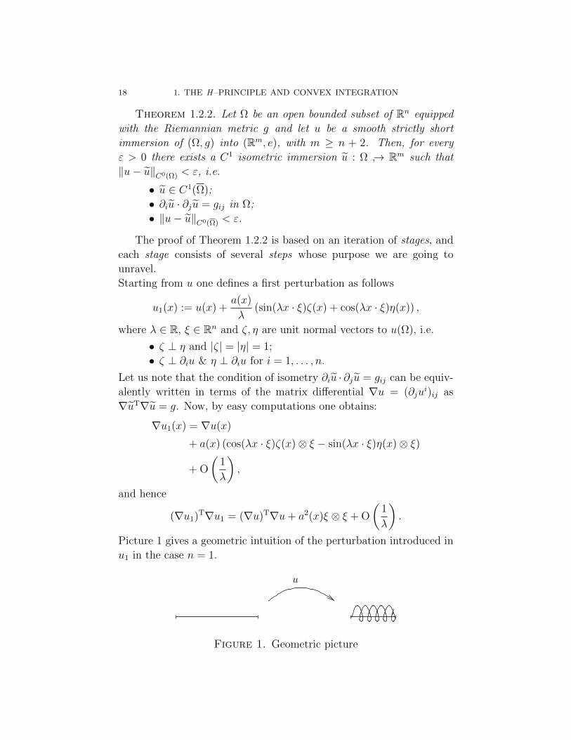
Starting from u one defines a first perturbation as follows
u1(x) := u(x) +a(x)
λ(sin(λx · ξ)ζ(x) + cos(λx · ξ)η(x)) ,
where λ ∈ R, ξ ∈ Rn and ζ, η are unit normal vectors to u(Ω), i.e.
• ζ ⊥ η and |ζ| = |η| = 1;
• ζ ⊥ ∂iu & η ⊥ ∂iu for i = 1, . . . , n.
Let us note that the condition of isometry ∂iu · ∂ju = gij can be equiv-
alently written in terms of the matrix differential ∇u = (∂jui)ij as
∇uT∇u = g. Now, by easy computations one obtains:
∇u1(x) = ∇u(x)
+ a(x) (cos(λx · ξ)ζ(x)⊗ ξ − sin(λx · ξ)η(x)⊗ ξ)
+ O
(1
λ
),
and hence
(∇u1)T∇u1 = (∇u)T∇u+ a2(x)ξ ⊗ ξ + O
(1
λ
).
Picture 1 gives a geometric intuition of the perturbation introduced in
u1 in the case n = 1.
u
Figure 1. Geometric picture

1.2. THE H -PRINCIPLE FOR ISOMETRIC EMBEDDINGS 19
Now, the purpose of a stage is to correct the error g − u]e =
u − (∇u)T∇u. In order to achieve this correction, the error is locally
decomposed into a sum of primitive metrics as follows
g − (∇u)T∇u =n∗∑k=1
a2kξk ⊗ ξk (locally).
Therefore, by iterating the procedure illustrated in the construction of
u1, i.e. by adding repeatedly ”spirally perturbations” to u it should be
possible to achieve uN such that
• (∇uN)T∇uN = g + O(
1λ
);
• ‖∇uN −∇u‖C0(Ω) =∑
k ‖ak‖C0(Ω)+O(
1λ
)∼∥∥g − (∇u)T∇u
∥∥1/2
C0(Ω);
• ‖uN − u‖C0(Ω) = O(
1λ
).
Let us draw the attention to the fact that, when introducing a per-
turbation as in u1, a, ζ and η may vary as x varies but that is not
the case for ξ which is a fixed vector: this prevents us from correcting
the error simply by taking the eigenvectors of g(x) − ∇u(x)T∇u(x).
This involves the use of a “partition of unity” of the set of positive
definite matrices. which we will not expound here. The previous con-
siderations show which kind of estimates are involved when adding a
primitive metric. Hence, the general Nash-Kuiper’s scheme lies in the
following iterations:
• step: a step involves adding one primitive metric; in other
words the goal of a step is the metric change
u]e→ u]e+∑
a2ξ ⊗ ξ;
• stage: a stage consists in decomposing the error into primitive
metrics and adding them successively in steps.
The number of steps in a stage equals the number of primitive metrics
in the above decomposition which interact. This equals n∗ for the
local construction and (n+ 1)n∗ for the global construction. Therefore
iterating the estimates for one step over a single stage and then over
the stages leads to the desired result.
1.2.3. Connection to the Euler equations. There is an inter-
esting analogy between isometric immersions in low codimension and
the incompressible and compressible Euler equations. In [DLS09] a
method, which is very closely related to convex integration, was intro-
duced to construct highly irregular energy-dissipating solutions of the

20 1. THE H –PRINCIPLE AND CONVEX INTEGRATION
incompressible Euler equations. In general the regularity of solutions
obtained using convex integration agrees with the highest derivatives
appearing in the equations. Being in conservation form, the “expected”
regularity space for convex integration for the incompressible Euler
equations should be C0. In [DLS09] a weaker version of convex inte-
gration was applied, to produce solutions in L∞ (see also [DLS10] for a
slightly better space) and to show that a weak version of the h-principle
holds (even if there is no homotopy there). Recently, De Lellis and
Szekelyhidi have proved the existence of continuous and even Holder
continuous solutions which dissipate the kinetic energy. Moreover the
same method devised in [DLS10] led to new developments in fluid
dynamics in particular for the Euler system of isentropic compressible
gas dynamics. When comparing the Euler equations (both compress-
ible and incompressible) and the Nash-Kuiper result, the reader should
take into account that, in this analogy, the velocity field of the Euler
equations corresponds to the differential of the embedding in the iso-
metric embedding problem. All these aspects are surveyed in the note
[DLS11].
The understanding of Nash’s construction is in a way a starting
point for the approach developed by De Lellis and Szekelyhidi in [DLS09].
As in the case of Nash, the solution of the incompressible Euler equa-
tions is generated by an iteration scheme: at each stage of this iteration
a subsolution is produced from the previous one by adding some special
perturbations, which oscillate quite fast. Hence, the final result of the
iteration scheme is the superposition of infinitely many perturbations
which converge suitably to an exact solution.
1.3. The h-principle and the equations of fluid dynamics
In a recent note [DLS11], De Lellis and Szekelyhidi disclosed the
analogy between recent outcomes in fluid dynamics (included the ones
presented in this thesis) and some h-principle-type results in differen-
tial geometry, as the previously presented Nash-Kuiper Theorem. More
precisely, the survey by De Lellis and Szekelyhidi aims at showing how
the theorems in fluid mechanics represent a suitable variant of Gro-
mov’s h-principle. In this section, we will retrace the main points of
[DLS11] so to place the results of this thesis in a more general context.
1.3. THE H -PRINCIPLE AND THE EQUATIONS OF FLUID DYNAMICS 21
1.3.1. The general framework. Kirchheim, Muller and Sverak
in [KMS03] outlined an approach to study the properties of nonlinear
partial differential equations through the geometric properties of a set
in the space of m × n matrices which is naturally associated to the
equation. This approach draws heavily on Tartar’s work on oscillations
in nonlinear PDEs and compensated compactness and on Gromov’s
work on partial differential relations and convex integration.
What does this method consist of? Following Tartar’s framework
[Tar79], many nonlinear systems of PDEs for a map u : Ω ⊂ Rn → Rd
can be naturally espressed as a combination of a linear system of PDEs
of the form
(1.2)n∑i=1
Ai∂iz = 0 in Ω
and a pointwise nonlinear constraint
(1.3) z(x) ∈ K a.e. x ∈ Ω,
where
• z : Ω ⊂ Rn → Rd is the unknown state variable;
• Ai are constant m× d matrices;
• K ⊂ Rd is a closed set.
Plane waves are solutions of (1.2) of the form
(1.4) z(x) = ah(x · ξ),
where h : R → R. Then, one defines the wave cone Λ related to one–
dimensional solutions and given by the states a ∈ Rd such that for any
choice of the profile h the function (1.4) solves (1.2):
(1.5) Λ :=
a ∈ Rd : ∃ξ ∈ Rn \ 0 with
n∑i=1
ξiAia = 0
.
Equivalently Λ characterizes the directions of one–dimensional oscilla-
tions compatible with (1.2). Given a cone Λ we say that a set S is
Λ-convex if for any two points A,B ∈ S with B − A ∈ Λ the whole
segment [A,B] belongs to S. The Λ-convex hull of K, KΛ, is the small-
est Λ-convex set containing K. In some sense the Λ-convex hull KΛ
constitutes a relaxation of the initial set K. Then one defines subsolu-
tions as solutions of the relaxed system, i.e. as solutions z of the linear
relations (1.2) which satisfy the relaxed condition z ∈ KΛ. Already
22 1. THE H –PRINCIPLE AND CONVEX INTEGRATION
at this stage, the concept of subsolutions is reminiscent of the previ-
ously introduced concept of short maps for the isometric embedding
problem. More precisely, equations (1.1) which define an isometric im-
mersion u can be formulated for the deformation gradient A := ∇u as
the coupling of the linear constraint
curlA = 0
with the nonlinear relation
ATA = g.
With this interpretation, short maps are “subsolutions” to the isometric
embedding problem.
The method of convex integration introduced by Gromov repre-
sents a generalization of Nash-Kuiper’s result and is based on the up-
shot that (1.2)-(1.3) admit many interesting solutions if KΛ is “big
enough”. Indeed, the key point of convex integration is to reintroduce
oscillations by adding suitable localized versions of (1.4) to the subso-
lutions and to recover a solution of (1.2)-(1.3) iterating this process.
The idea of adding oscillatory perturbations can be implemented either
in an “implicite” way by the so called Baire category method or in a
more constructive way. Both approaches provide the key to prove some
h-principle-type results for systems of nonlinear evolutionary partial
differential equations: they allow to show that, under suitable assump-
tions on the relaxed set KΛ, the existence of subsolutions leads to the
existence of solutions.
1.3.1.1. Baire category method. The Baire category method is a
method of enforcing the idea of convex integration and relies on the
surprising fact that, in a Baire generic sense, most solutions of the
“relaxed system”, i.e. most subsolutions, are actually solutions of the
original system. Here, we recall the main steps underlying this ap-
proach following the “jargon” introduced by Kirchheim in [Kir03] (see
also [DLS11]). In Kirchheim’s formalisation, the space of subsolutions
arises from a nontrivial open set U ⊂ Rd (U plays the role of KΛ in the
previous section) satisfying the following perturbation property.
Perturbation Property (P): There is a continuous function ε :
R+ → R+ with ε(0) = 0 with the following property: for every z ∈ Uthere is a sequence of solutions zj ∈ C∞c (B1) of (1.2) such that

1.3. THE H -PRINCIPLE AND THE EQUATIONS OF FLUID DYNAMICS 23
• zj 0 weakly in L2(Rn);
• z + zj(x) ∈ U ∀x ∈ Rn;
•∫|zj(x)|2 dx ≥ ε(dist(z,K)).
The set U should be thought of as a relaxation of the initial set K,
which, according to Kirchheim’s jargon, “is stable only near K”. Next,
define X0 as follows
X0 := z ∈ C∞c (Ω) : z satisfies (1.2) and z(x) ∈ U for all x ∈ Ω ,
so that X0 is the set of smooth compactly supported subsolutions of
(1.2)-(1.3). Thanks to the perturbation property, X0 consists of func-
tions which are perturbable in an open subdomain O ⊂ Ω. Then let X
be the closure of X0 with respect to the weak L2-topology. Assuming
that K is bounded, the set X0 is bounded in L2 and the topology of
weak L2 convergence is metrizable on X, making it into a complete
space. Denote its metric by dX(·, ·). An easy covering argument, to-
gether with property (P), results in the following lemma:
Lemma 1.3.1. There is a continuous function ε : R+ → R with
ε(0) = 0 such that for every z ∈ X0 there is a sequence zj ∈ X0 with
zjdX→ z in X and∫
Ω
|zj − z|2 dx ≥ ε
(∫Ω
dist(z(x), K)dx
).
Since the map I : z 7→∫
Ω|z|2 dx is a Baire 1-function on X, an easy
application of the Baire category theorem gives that the set
Y := z ∈ X : I is continuous at z
is residual in X. By virtue of the previous lemma we can prove that
z ∈ Y implies z(x) ∈ K for almost every x ∈ Ω:
Theorem 1.3.2. Assuming the perturbation property to hold, the
set
Z := z ∈ X : z(x) ∈ K a.e. x ∈ Ωis residual in X.
Proof . In order to prove Theorem 1.3.2 it suffices to show that
Y ⊂ Z. We will proceed by contradiction. So, let z ∈ Y and let
zj ∈ X0 such that zjdX→ z in X. Now, let us assume by absurd that∫
Ωdist(z(x), K)dx =: δ > 0. Thanks to lemma 1.3.1 we can pass (up

24 1. THE H –PRINCIPLE AND CONVEX INTEGRATION
to a diagonal argument) to a new sequence zj with zjdX→ z and such
that
(1.6)
∫Ω
|zj − zj|2 dx ≥ ε
(∫Ω
dist(zj(x), K)dx
).
Since z is a point of continuity of I, it follows that zj → z strongly in
L2 as well as zj → z strongly in L2. This implies in particular that
(1.7)
∫Ω
|zj − zj|2 dx→ 0 as j → +∞.
Moreover the strong convergence in L2 of the sequence zj to z together
with the hypothesis of absurd, allow us assume to that, from a certain
j on,∫
Ωdist(zj(x), K)dx > δ/2 > 0 whence ε
(∫Ω
dist(zj(x), K)dx)>
α > 0 for every j > j and for some α. This inequality together with
(1.7) contradicts (1.6).
1.3.1.2. Constructive convex integration. In the previous section we
presented the so called Baire category method, which is in some sense
non contructive. However, the same idea of adding oscillatory pertur-
bations can be implemented in a constructive way as well. In a nutshell
the idea is to define a sequence of subsolutions zk ∈ KΛ recursively as
(1.8) zk+1(x) = zk(x) + Zk(x, λkx),
where
Zk(x, ξ)
is a periodic plane-wave (see (1.4)) solution of (1.2) in the variable ξ,
parametrized by x and λk is a large frequency to be chosen. The aim
is to choose the plane-wave Zk and the frequency λk iteratively in such
a way that
• zk continues to satisfy (1.2) (strictly speaking this requires an
additional corrector term in the scheme (1.8));
• zk belongs to the relaxed constitutive set KΛ;
• zk → z in L2(Ω) with z ∈ K a.e..
The convergence of this constructive scheme is improved by choosing
the frequencies λk higher and higher. On the other hand clearly any
(fractional) derivative or Holder norm of zk gets worse by such a choice
of λk. The best regularity corresponds to the slowest rate at which the
frequencies λk tend to infinity while still leading to convergence.
1.3. THE H -PRINCIPLE AND THE EQUATIONS OF FLUID DYNAMICS 25
1.3.2. Non–standard solutions in fluid dynamics.
1.3.2.1. Incompressible Euler equations: non-uniqueness results. The
first and leading example of the h-principle in the realm of fluid dy-
namics is due to De Lellis and Szekelyhidi and pertains to the incom-
pressible Euler equations:
(1.9)
divxv = 0
∂tv + divx (v ⊗ v) +∇xp = 0
v(·, 0) = v0
.
Here the unknowns v and p are, respectively, a vector field and a
scalar field defined on Rn × [0, T ). These fundamental equations were
derived 250 years ago by Euler and since then have played a major role
in fluid dynamics. There are several outstanding problems connected to
(1.9). In particular, weak solutions are known to be badly behaved in
the sense of Hadamard’s well-posedness: in the groundbreaking paper
[Sch93] proved the existence of a nontrivial weak solution compactly
supported in time. Thanks to the intuition of De Lellis and Szekelyhidi
such a nonuniqueness result has been explained as a suitable variant
of the original h-principle by use of the method of convex integration.
Moreover, such an approach allowed them to go way beyond the result
of Scheffer and it has lead to new developments for several equations
in fluid dynamics included the one presented in this work.
As already mentioned, the first nonuniqueness result for weak so-
lutions of (1.9) is due to Scheffer in [Sch93]. The main theorem of
[Sch93] states the existence of a nontrivial weak solution in L2(R2×R)
with compact support in space and time. Later on Shnirelman in
[Shn97] gave a different proof of the existence of a nontrivial weak
solution in space-periodic setting and with compact support in time.
In these constructions it is not clear wheter the solution belongs to
the energy space. In the paper [DLS09], De Lellis and Szekelyhidi
provided a relatively simple proof of the following stronger statement.
Theorem 1.3.3 (Non-uniqueness of weak solutions to the incom-
pressible Euler equations). There exist infinitely many compactly sup-
ported weak solutions of the incompressible Euler equations (1.9) in any
space dimension greater or equal to 2. In particular there are infinitely
many solutions v ∈ L∞ ∩ L2 to (1.9) for v0 = 0 and arbitrary n ≥ 2.
The proof of Theorem 1.3.3 is based on the notion of subsolution.
The spirit behind the notion of subsolutions in this context is the same

26 1. THE H –PRINCIPLE AND CONVEX INTEGRATION
as the one outlined in the previous sections for general evolutionary par-
tial differential equations. On the other hand, the definition of subsolu-
tion for the incompressible Euler system (1.9) can be made explicit and
can be motivated in terms of the Reynold stress (see [DLS11] for more
details on the connection between Reynold stress and subsolutions). In
particular, if one writes (1.9) as the coupling of a linear system of PDEs
and a pointwise non-linear constraint (as in (1.2)-(1.3)), then subsolu-
tions are solutions of this linear system which belong pointwise to the
convex hull of the non-linear constraint set. In other words:
Definition 1.3.4 (Subsolution of incompressible Euler). Let e ∈L1loc(Rn× (0, T )) with e ≥ 0. A subsolution to the incompressible Euler
equations with given kinetic energy density e is a triple
(v, u, q) : Rn × (0, T )→ Rn × Sn×n0 × R
with the following properties:
• v ∈ L2loc, u ∈ L1
loc, q is a distribution;
•
(1.10)
divxv = 0
∂tv + divxu+∇xq = 0
in the sense of distributions;
•v ⊗ v − u ≤ 2
neId a.e.
Observe that subsolutions automatically satisfy 12|v|2 ≤ e a.e. If in
addition, the equality sign 12|v|2 = e a.e. holds true, then the v compo-
nent of the subsolution is in fact a weak solution of the incompressible
Euler equations. From the previous definition we can grasp even better
the analogy between the velocity field of the Euler equations and the
differential of the embedding in the isometric embedding problem and
hence between subsolutions and short maps. Also the heuristic behind
the two results shows striking similarities. The key point in De Lellis
and Szekelyhidi’s approach to prove Theorem 1.3.3 is that, starting
from a subsolution, an appropriate iteration process reintroduce the
high frequencies oscillations. In the limit of this process one obtains
weak solutions to (1.9). However, since the oscillations are reintroduced
in a very non-unique way, in fact this generates several solutions from
the same subsolution. The relevant iteration scheme has been already

1.3. THE H -PRINCIPLE AND THE EQUATIONS OF FLUID DYNAMICS 27
outlined in the general setting in Section 1.3.1. The following theorem
comes from Proposition 2 in [DLS10] and is a precise formulation of
the previous discussion.
Theorem 1.3.5 (Subsolution criterion). Let e ∈ C(Rn × (0, T ))
and (v, u, q) a smooth, strict subsolution, i.e.
(v, u, q) ∈ C∞(Rn × (0, T )) satisfies (1.10)
and
(1.11) v ⊗ v − u < 2
neId a.e. on Rn × (0, T ).
Then there exist infinitely many weak solutions v ∈ L∞loc(Rn× (0, T )) of
the incompressible Euler equations (1.9) with pressure p = q − 2ne and
such that1
2|v|2 = e
for a.e. (x, t). Infinitely many among these belong to C((0, T ), L2). If
in addition
v(·, t) v0(·) in L2loc(Rn) as t→ 0,
then all the v’s so constructed solve (1.9).
The previous results show that weak solutions of the Euler equa-
tions are in general highly non-unique. Moreover the kinetic energy
density 12|v|2 can be prescribed as an independent quantity. Since
classical C1 solutions of the incompressible Euler equations are char-
acterized by conservation of the total kinetic energy
d
dt
∫Rn
|v|2
2(x, t)dx = 0,
one can complement the notion of weak solution to (1.9) with several
admissibility criteria defined as “relaxations” (in a proper sense) of
the energy conservation. Let us denote by L2w(Rn) the space L2(Rn)
endowed with the weak topology. We recall that any weak solution
of (1.9) can be modified on a set of measure zero so to get v ∈C([0, T ), L2
w(Rn)). Consequently v has a well-defined trace at every
time. This allows to introduce the following admissibility criteria for
weak solutions:
(a) ∫|v|2 (x, t)dx ≤
∫|v0|2 (x)dx for every t.

28 1. THE H –PRINCIPLE AND CONVEX INTEGRATION
(b) ∫|v|2 (x, t)dx ≤
∫|v|2 (x, s)dx for every t > s.
(c) If in addition v ∈ L3loc, then
∂t|v|2
2+ div
((|v|2
2+ p
)v
)≤ 0
in the sense of distributions.
The first two criteria are of course suggested by the conservation of
kinetic energy of classical solutions, while condition (c) has been pro-
posed for the first time by Duchon and Robert in [DR00] and it re-
sembles the admissibility criteria which are popular in the literature on
hyperbolic conservation laws. However, none of these criteria restore
the uniqueness of weak solutions.
Theorem 1.3.6 (Non-uniqueness of admissible weak solutions to
the incompressible Euler equations). There exist initial data v0 ∈ L∞∩L2 for which there are infinitely many bounded solutions of (1.9) which
are strongly L2-continuous and satisfy (a), (b) and (c).
The conditions (a), (b) and (c) hold with the equality sign for in-
finitely many of these solutions, whereas for infinitely many other they
hold as strict inequalities.
This theorem has been stated and proved in [DLS10]. The sec-
ond part of the statement generalizes the intricate construction of
Shnirelman in [Shn97], which produced the first example of a weak
solution in 3d of (1.9) with strict inequalities in (a) and (b).
1.3.2.2. Incompressible Euler equations: h-principle. De Lellis and
Szekelyhidi in [DLS12] were able to extend the previous results: they
devised a new iteration scheme which produces continuous and even
Holder continuous solutions on T3. Indeed, for the incompressible Euler
equations, the natural space for convex integration is C0. The method
used in [DLS09] producing solutions in L∞ was a weak form of convex
integration. The new iteration scheme of [DLS12] is closer to the
approach of Nash [Nas54] for the isometric embedding problem.
Recently, A. Choffrut [Cho12] established optimal h-principles in
two and three space dimensions. More specifically he identifies all

1.3. THE H -PRINCIPLE AND THE EQUATIONS OF FLUID DYNAMICS 29
subsolutions (defined in a suitable sense) which can be approximated in
the H1-norm by exact solutions of the incompressible Euler equations.
For the precise statement we refer the reader directly to [Cho12].
1.3.2.3. Incompressible Euler equations: Wild initial data. The ini-
tial data v0 constructed in Theorem 1.3.6 are obviously not regular,
since for regular initial data the local existence theorems and the weak-
strong uniqueness (see [BDLS11]) ensure local uniqueness under con-
dition (a). One might therefore ask how large is the set of these “wild”
initial data. A consequence of De Lellis and Szekelyhidi’s method is
the following density theorem proved by Szekelyhidi and Wiedemann
in [SW11].
Theorem 1.3.7 (Density of wild initial data). The set of initial
data v0 for which the conclusions of Theorem 1.3.6 holds is dense in
the space of L2 solenoidal vectorfields.
Another surprising corollary is that the usual shear flow is a “wild
initial datum”. More precisely, if we consider the following solenoidal
vector field in R2
(1.12) v0(x) :=
(1, 0) if x2 > 0,
(−1, 0) if x2 < 0,
then:
Theorem 1.3.8 (Wild vortex sheet). For v0 as in (1.12), there are
infitely many weak solutions of (1.9) on R2 × [0,∞) which satisfy (c).
This theorem has been proven in [Sz1] using Proposition 1.3.5 and
hence the proof amounts to showing the existence of a suitable subso-
lution. We will further discuss this result in Chapter 3.
1.3.2.4. Incompressible Euler equations: global existence of weak so-
lutions. A further application of Theorem (1.3.5) is due to Wiedemann
[Wie11]. E. Wiedemann considered an arbitrary initial datum v0 ∈L2loc(Rn) and constructed a smooth triple (v, u, q) ∈ C∞(Rn × (0, T ))
which solves (1.10) with initial datum v0 and is a subsolution for a
proper choice of the profile of e. In particular, by constructing a subso-
lution with bounded energy, Wiedemann in [Wie11] recently obtained
the following:
30 1. THE H –PRINCIPLE AND CONVEX INTEGRATION
Corollary 1.3.9 (Global existence for weak solutions). Let v0 ∈L2(Tn) be a solenoidal vector field. Then there exist infinitely many
global weak solutions of (1.9) with bounded energy.
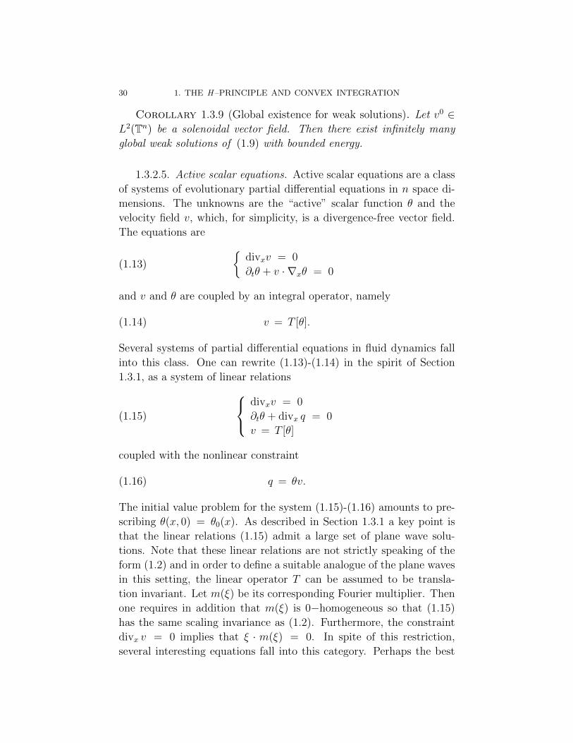
1.3.2.5. Active scalar equations. Active scalar equations are a class
of systems of evolutionary partial differential equations in n space di-
mensions. The unknowns are the “active” scalar function θ and the
velocity field v, which, for simplicity, is a divergence-free vector field.
The equations are
(1.13)
divxv = 0
∂tθ + v · ∇xθ = 0
and v and θ are coupled by an integral operator, namely
(1.14) v = T [θ].
Several systems of partial differential equations in fluid dynamics fall
into this class. One can rewrite (1.13)-(1.14) in the spirit of Section
1.3.1, as a system of linear relations
(1.15)
divxv = 0
∂tθ + divx q = 0
v = T [θ]
coupled with the nonlinear constraint
(1.16) q = θv.
The initial value problem for the system (1.15)-(1.16) amounts to pre-
scribing θ(x, 0) = θ0(x). As described in Section 1.3.1 a key point is
that the linear relations (1.15) admit a large set of plane wave solu-
tions. Note that these linear relations are not strictly speaking of the
form (1.2) and in order to define a suitable analogue of the plane waves
in this setting, the linear operator T can be assumed to be transla-
tion invariant. Let m(ξ) be its corresponding Fourier multiplier. Then
one requires in addition that m(ξ) is 0−homogeneous so that (1.15)
has the same scaling invariance as (1.2). Furthermore, the constraint
divx v = 0 implies that ξ · m(ξ) = 0. In spite of this restriction,
several interesting equations fall into this category. Perhaps the best

1.3. THE H -PRINCIPLE AND THE EQUATIONS OF FLUID DYNAMICS 31
known examples are the surface quasi geostrophic and the incompress-
ible porous medium equations, corresponding respectively to
m(ξ) = i |ξ|−1 (−ξ2, ξ1) and(1.17)
m(ξ) = |ξ|−2 (ξ1ξ2,−ξ21).(1.18)
In [CFG09] Cordoba, Faraco and Gancedo proved the following theo-
rem.
Theorem 1.3.10. Assume m is given by (1.18). Then there exist
infinitely many weak solutions of (1.15) and (1.16) in L∞(T2×[0,+∞[)
with θ0 = 0.
This was generalized by Shvydkoy to all even m(ξ) satisfying a
mild additional regularity assumption. We refer to the original paper
[Shv11] for the details.
The proof of Theorem 1.3.10 in [CFG09], as well as the proof by
Shvydkoy in [Shv11], relies on some refined tools which were devel-
oped in the theory of laminates and differential inclusions and they
present some substantial differences with the methods of De Lellis and
Szekelyhidi in [DLS09] and [DLS10]. Indeed, the method used in
[CFG09] is still based on understanding the equation as a differen-
tial inclusion in the spirit of Tartar [Tar79], but in the context of
the porous media equation the situation differs from the setting of
[DLS09]-[DLS10] and the authors had to take different routes in sev-
eral steps. First, we would like to recall that a central point is to find
an open set U satisfying the perturbation property (P). One possible
candidate would be to take the largest open set Umax satisfying (P).
Obviously this set is particularly meaningful since it gives the largest
possible space X for which genericity conclusions holds. Moreover, this
has the advantage that - at least in many relevant cases - the set Umaxcoincides with the interior of the Λ–convex hull KΛ, which in turn can
be characterized by separation arguments. For instance, in Theorem
1.3.5 condition (1.11) characterizes precisely the interior of KΛ. Fur-
thermore, in this case the interior of KΛ is the interior of the convex
hull Kco.
In [CFG09] and [Shv11] the authors avoid calculating the full Λ–
convex hull and instead restrict themselves to exhibiting a nontrivial
(but possibly much smaller) open set U satisfying (P). Opposite to

32 1. THE H –PRINCIPLE AND CONVEX INTEGRATION
the incompressible Euler equations, in [CFG09] and [Shv11] the Λ–
convex hull does not agree with the convex hull and more relevant
K ⊂ ∂KΛ. This is of course an obstruction for the available versions
of convex integration as presented in Section 1.3.1 (the ones based
on Baire category and the direct constructions). So the argument in
[CFG09] and [Shv11] suggests a more systematic approach: instead
of fixing a set and computing the hull, they pick a reasonable matrix A
and compute (A+ Λ)∩K. Then by the results in [Kir03] it is enough
to find a set K ⊂ (A + Λ) ∩ K such that A ∈ Kco to find what are
called degenerate T4 configurations (see [KMS03]) supported in Kco).
However, in exchange they are forced to use much more complicated
sequences zj. Indeed, the zj’s used in [DLS10] are localizations of
simple plane waves, whereas the ones used in [CFG09] and [Shv11]
arise as an infinite nested sequence of repeated plane waves.
The obvious advantage of the method introduced in [CFG09] and
used in [Shv11] is that it seems to be fairly robust and general. It is
useful in cases where an explicit computation of the hull KΛ is out of
reach due to the high complexity and high dimensionality. Anyway, the
constructions carried out in this dissertation are analogue to the ones
by De Lellis and Szekelyhidi and they do not require any understanding
of the ideas by [CFG09] and [Shv11].
CHAPTER 2
Non–uniqueness with arbitrary density
In this chapter we present and prove the first result stated in the
Introduction of the thesis, i.e. Theorem 0.2.1: given any continuosly
differentiable initial density, we can construct bounded initial momenta
for which admissible solutions to the isentropic compressible Euler
equations are not unique in more than one space dimension.
The content of this chapter corresponds to the subject of the paper
[Chi11] written by the author during the PhD studies. In particular
the structure of the chapter is as follows. In the first section, we in-
troduce the problem and the setting we will work with and we state
the main result: even if the equations under investigation have already
been presented in the Introduction of the thesis, we chose to recall
them herein so that the chapter will be self-contained. Section 2 is
an overview on the definitions of weak and admissible solutions and
gives a first glimpse on how Theorem 0.2.1 is achieved. Section 3 is
devoted to the reformulation of a simplified version of the isentropic
compressible Euler equations as a differential inclusion and to the cor-
responding geometrical analysis. In Section 4 we state and prove a
criterion (Proposition 2.4.1) to select initial momenta allowing for in-
finitely many solutions. The proof builds upon a refined version of the
Baire category method for differential inclusions developed in [DLS10]
and aimed at yielding weakly continuous in time solutions. Section 5
and 6 contain the proofs of the main tools used to prove Proposition
2.4.1. In Section 7, we show initial momenta satisfying the require-
ments of Proposition 2.4.1. Finally, in Section 8 we prove Theorem
0.2.1 (here stated in the first section as Theorem 2.1.1) by applying
Proposition 2.4.1.
2.1. Introduction
We deal with the Cauchy Problem for the isentropic compressible
Euler equations in the space-periodic setting.
33
34 2. NON–UNIQUENESS WITH ARBITRARY DENSITY
We first introduce the isentropic compressible Euler equations of gas
dynamics in n space dimensions, n ≥ 2 (cf. Section 3.3 of [Daf00]).
They are obtained as a simplification of the full compressible Euler
equations, by assuming the entropy to be constant. The state of the
gas will be described through the state vector
V = (ρ,m)
whose components are the density ρ and the linear momentum m. In
contrast with the formulation of the problem given in the Introduction
of the thesis, here the equations are written in terms of the linear
momentum field which allows to write the equations in the canonical
form (see [Daf00]). The balance laws in force are for mass and linear
momentum. The resulting system, which consists of n + 1 equations,
takes the form (cf. (0.1)):
(2.1)
∂tρ+ divxm = 0
∂tm+ divx
(m⊗mρ
)+∇x[p(ρ)] = 0
ρ(·, 0) = ρ0
m(·, 0) = m0
.
The pressure p is a function of ρ determined from the constitutive
thermodynamic relations of the gas in question. A common choice is
the polytropic pressure law
p(ρ) = kργ
with constants k > 0 and γ > 1. The set of admissible values is
P = ρ > 0 (cf. [Daf00] and [Ser99]). As already explained, the
system is hyperbolic if
p′(ρ) > 0.
In addition, thermodynamically admissible processes must also satisfy
an additional constraint coming from the energy inequality
(2.2) ∂t
(ρε(ρ) +
1
2
|m|2
ρ
)+ divx
[(ε(ρ) +
1
2
|m|2
ρ2+p(ρ)
ρ
)m
]≤ 0
where the internal energy ε : R+ → R is given through the law p(r) =
r2ε′(r). The physical region for (2.1) is (ρ,m)| |m| ≤ Rρ, for some
constant R > 0. For ρ > 0, v = m/ρ represents the velocity of the
fluid.

2.2. WEAK AND ADMISSIBLE SOLUTIONS 35
We will consider, from now on, the case of general pressure laws
given by a function p on [0,∞[, that we always assume to be continu-
ously differentiable on [0,∞[. The crucial requirement we impose upon
p is that it has to be strictly increasing on [0,∞[. Such a condition is
meaningful from a physical viewpoint since it is a consequence of the
principles of thermodynamics.
Using some techniques introduced by De Lellis-Szekelyhidi (cf. [DLS09]
and [DLS10]) we can consider any continuously differentiable periodic
initial density ρ0 and exhibit suitable periodic initial momenta m0 for
which space-periodic weak admissible solutions of (2.1) are not unique
on some finite time-interval.
Theorem 2.1.1. Let n ≥ 2. Then, for any given function p and
any given continuously differentiable periodic initial density ρ0, there
exist a bounded periodic initial momentum m0 and a positive time T
for which there are infinitely many space-periodic admissible solutions
(ρ,m) of (2.1) on Rn × [0, T [ with ρ ∈ C1(Rn × [0, T [).
Remark 2.1.2. Indeed, in order to prove Theorem 2.1.1, it would
be enough to assume that the initial density is a Holder continuous
periodic function: ρ0 ∈ C0,α(Rn) (cf. Proof of Proposition 2.7.1).
Some connected results are obtained in [DLS10] (cf. Theorem 2
therein) as a further consequence of their analysis on the incompressible
Euler equations. Inspired by their approach, we adapt and apply di-
rectly to (2.1) the method of convex integration combined with Tartar’s
programme on oscillation phenomena in conservation laws (see [Tar79]
and [KMS03]). In this way, we can show failure of uniqueness of ad-
missible solutions to the compressible Euler equations starting from
any given continuously differentiable initial density.
2.2. Weak and admissible solutions to
the isentropic Euler system
The deceivingly simple-looking system of first-order partial differ-
ential equations (2.1) has a long history of important contributions over
more than two centuries. We recall a few classical facts on this system
(see for instance [Daf00] for more details).
• If ρ0 and m0 are “smooth” enough (see Theorem 5.3.1 in
[Daf00]), there exists a maximal time interval [0, T [ on which
36 2. NON–UNIQUENESS WITH ARBITRARY DENSITY
there exists a unique “smooth” solution (ρ,m) of (2.1) (for
0 ≤ t < T ). In addition, if T < ∞, and this is the case in
general, (ρ,m) becomes discontinuous as t goes to T .
• If we allow for discontinuous solutions, i.e., for instance, solu-
tions (ρ,m) ∈ L∞ satisfying (2.1) in the sense of distributions,
then solutions are neither unique nor stable. More precisely,
one can exhibit sequences of such solutions which converge
weakly in L∞ − ∗ to functions which do not satisfy (2.1).
• In order to restore the stability of solutions and (possibly) the
uniqueness, one may and should impose further restrictions
on bounded solutions of (2.1), restrictions which are known as
(Lax) entropy inequalities.
In this chapter we address the problem of better understanding
the efficiency of entropy inequalities as selection criteria among weak
solutions.
Here, we have chosen to emphasize the case of the flow with space
periodic boundary conditions. For space periodic flows we assume that
the fluid fills the entire space Rn but with the condition that m, ρ are
periodic functions of the space variable. The space periodic case is
not a physically achievable one, but it is relevant on the physical side
as a model for some flows. On the mathematical side, it retains the
complexities due to the nonlinear terms (introduced by the kinematics)
and therefore it includes many of the difficulties encountered in the
general case. However the former is simpler to treat because of the
absence of boundaries. Furthermore, using Fourier transform as a tool
simplifies the analysis.
Let Q = [0, 1]n, n ≥ 2 be the unit cube in Rn. We denote by
Hmp (Q), m ∈ N, the space of functions which are in Hm
loc(Rn) and
which are periodic with period Q:
m(x+ l) = m(x) for a.e. x ∈ Rn and every l ∈ Zn.
For m = 0, H0p (Q) coincides simply with L2(Q). Analogously, for every
functional space X we define Xp(Q) to be the space of functions which
are locally (over Rn) in X and are periodic of period Q. The functions
in Hmp (Q) are easily characterized by their Fourier series expansion
(2.3)
Hmp (Q) =
m ∈ L2
p(Q) :∑k∈Zn
|k|2m |m(k)|2 <∞ and m(0) = 0
,

2.2. WEAK AND ADMISSIBLE SOLUTIONS 37
where m : Zn → Cn denotes the Fourier transform of m. We will use
the notation H(Q) for H0p (Q) and Hw(Q) for the space H(Q) endowed
with the weak L2 topology.
Let T be a fixed positive time. By a weak solution of (2.1) on
Rn × [0, T [ we mean a pair (ρ,m) ∈ L∞([0, T [;L∞p (Q)) satisfying
(2.4)
|m(x, t)| ≤ Rρ(x, t) for a.e. (x, t) ∈ Rn × [0, T [ and some R > 0,
and such that the following identities hold for every test functions ψ ∈C∞c ([0, T [;C∞p (Q)), φ ∈ C∞c ([0, T [;C∞p (Q)):
(2.5)
∫ T
0
∫Q
[ρ∂tψ +m · ∇xψ] dxdt+
∫Q
ρ0(x)ψ(x, 0)dx = 0
∫ T
0
∫Q
[m · ∂tφ+
⟨m⊗mρ
,∇xφ
⟩+ p(ρ) divx φ
]dxdt
+
∫Q
m0(x) · φ(x, 0)dx = 0.(2.6)
For n ≥ 2 the only non-trivial entropy is the total energy η =
ρε(ρ)+12|m|2ρ
which corresponds to the flux Ψ =(ε(ρ) + 1
2|m|2ρ2
+ p(ρ)ρ
)m.
Then a bounded weak solution (ρ,m) of (2.1) satisfying (3.21) in
the sense of distributions, i.e. satisfying the following inequality∫ T
0
∫Q
[(ρε(ρ) +
1
2
|m|2
ρ
)∂tϕ+
(ε(ρ) +
1
2
|m|2
ρ2+p(ρ)
ρ
)m · ∇xϕ
]
+
∫Q
(ρ0ε(ρ0) +
1
2
|m0|2
ρ
)ϕ(·, 0) ≥ 0,
(2.7)
for every nonnegative ϕ ∈ C∞c ([0, T [;C∞p (Q)), is said to be an entropy
(or admissible) solution of (2.1).
The lack of entropies is one of the essential reasons for a very limited
understanding of compressible Euler equations in dimensions greater
than or equal to 2.
The recent paper [DLS10] by De Lellis-Szekelyhidi gives an ex-
ample in favour of the conjecture that entropy solutions to the multi-
dimensional compressible Euler equations are in general not unique:
see Theorem 0.1.1 in the Introduction of the thesis. Showing that this
conjecture is true has far-reaching consequences. The entropy condition
38 2. NON–UNIQUENESS WITH ARBITRARY DENSITY
is not sufficient as a selection principle for physical/unique solutions.
The non-uniqueness result by De Lellis-Szekelyhidi is a byproduct of
their new analysis of the incompressible Euler equations based on its
formulation as a differential inclusion. They first show that, for some
bounded compactly supported initial data, none of the classical admis-
sibility criteria singles out a unique solution to the Cauchy problem for
the incompressible Euler equations. As a consequence, by construct-
ing a piecewise constant in space and independent of time density ρ,
they look at the compressible isentropic system as a “piecewise incom-
pressible” system (i.e. still incompressible in the support of the veloc-
ity field) and thereby exploit the result for the incompressible Euler
equations to exhibit bounded initial density and bounded compactly
supported initial momenta for which admissible solutions of (2.1) are
not unique (in more than one space dimension).
Inspired by their techniques, we give a further counterexample to
the well-posedeness of entropy solutions to (2.1). Our result differs in
two main aspects: here the initial density can be any given “regular”
function and remains “regular” forward in time while in [DLS10] the
density allowing for infinitely many admissible solutions must be chosen
as piecewise constant in space; on the other hand we are not able to deal
with compactly supported momenta (indeed we work in the periodic
setting), hence our non-unique entropy solutions are only locally L2 in
contrast with the global-L2-in-space property of solutions obtained in
[DLS10]. Moreover, we have chosen to study the case of the flow in
a cube of Rn with space periodic boundary conditions. This case leads
to many technical simplifications while retaining the main structure of
the problem.
More precisely, we are able to analyze the compressible Euler equa-
tions in the framework of convex integration introduced in Chapter
1. We recall that this method works well with systems of nonlinear
PDEs such that the convex envelope (in an appropriate sense) of each
small domain of the submanifold representing the PDE in the jet-space
(see [EM02] for more details) is big enough. In our case, we consider
a simplification of system (2.1), namely the semi-stationary associated
problem, whose submanifold allows a convex integration approach lead-
ing us to recover the result of Theorem 2.1.1.
We are interested in the semi-stationary Cauchy problem associated
with the isentropic Euler equations (simply set to 0 the time derivative
2.2. WEAK AND ADMISSIBLE SOLUTIONS 39
of the density in (2.1) and drop the initial condition for ρ):
(2.8)
divxm = 0
∂tm+ divx
(m⊗mρ
)+∇x[p(ρ)] = 0
m(·, 0) = m0.
A pair (ρ,m) ∈ L∞p (Q)×L∞([0, T [;L∞p (Q)) is a weak solution on Rn×[0, T [ of (2.8) if m(·, t) is weakly-divergence free for almost every 0 <
t < T and satisfies the following bound
(2.9)
|m(x, t)| ≤ Rρ(x) for a.e. (x, t) ∈ Rn × [0, T [ and some R > 0,
and if the following identity holds for every φ ∈ C∞c ([0, T [;C∞p (Q)):∫ T
0
∫Q
[m · ∂tφ+
⟨m⊗mρ
,∇xφ
⟩+ p(ρ) divx φ
]dxdt
+
∫Q
m0(x) · φ(x, 0)dx = 0.(2.10)
A general observation suggests us that a non-uniqueness result for
weak solutions of (2.8) whose momentum’s magnitude satisfies some
suitable constraint could lead us to a non-uniqueness result for entropy
solutions of the isentropic Euler equations (2.1). Indeed, the entropy
solutions we construct in Theorem 2.1.1 come from some weak solutions
of (2.8).
Theorem 2.2.1. Let n ≥ 2. Then, for any given function p, any
given density ρ0 ∈ C1p(Q) and any given finite positive time T , there
exists a bounded initial momentum m0 for which there are infinitely
many weak solutions (ρ,m) ∈ C1p(Q) × C([0, T ];Hw(Q)) of (2.8) on
Rn × [0, T [ with density ρ(x) = ρ0(x).
In particular, the obtained weak solutions m satisfy
|m(x, t)|2 = ρ0(x)χ(t) a.e. in Rn × [0, T [,(2.11) ∣∣m0(x)∣∣2 = ρ0(x)χ(0) a.e. in Rn,(2.12)
for some smooth function χ.
An easy computation shows how, by properly choosing the function
χ in (2.11)-(2.12), the solutions (ρ0,m) of (2.8) obtained in Theorem
2.2.1 satisfy the admissibility condition (3.26).

40 2. NON–UNIQUENESS WITH ARBITRARY DENSITY
Theorem 2.2.2. Under the same assumptions of Theorem 2.2.1,
there exists a maximal time T > 0 such that the weak solutions (ρ,m) of
(2.8) (coming from Theorem 2.2.1) satisfy the admissibility condition
(3.26) on [0, T [.
Our construction yields initial data m0 for which the nonunique-
ness result of Theorem 2.1.1 holds on any time interval [0, T [, with
T ≤ T . However, as pointed out before, for sufficiently regular initial
data, classical results give the local uniqueness of smooth solutions.
Thus, a fortiori, the initial momenta considered in our examples have
necessarily a certain degree of irregularity.
2.3. Geometrical analysis
This section is devoted to a qualitative analysis of the isentropic
compressible Euler equations in a semi-stationary regime (i.e. (2.8)).
As in [DLS09] we will interpret the system (2.8) in terms of a differ-
ential inclusion, so that it can be studied in the framework combining
the plane wave analysis of Tartar, the convex integration of Gromov
and the Baire’s arguments. For a complete description of this general
framework we refer to Chapter 1, Section 1.3.1. In Section 2.3.2 we
will recall only the tools needed for our construction.
2.3.1. Differential inclusion. The system (2.8) can indeed be
naturally expressed as a linear system of partial differential equations
coupled with a pointwise nonlinear constraint, usually called differen-
tial inclusion.
The following Lemma, based on Lemma 2 in [DLS10], gives such
a reformulation. We will denote by Sn the space of symmetric n × nmatrices, by Sn0 the subspace of Sn of matrices with null trace, and by
In the n× n identity matrix.
Lemma 2.3.1. Let m ∈ L∞([0, T ];L∞p (Q;Rn)), U ∈ L∞([0, T ];L∞p (Q;Sn0 ))
and q ∈ L∞([0, T ];L∞(Q;R+)) such that
divxm = 0
∂tm+ divx U +∇xq = 0.(2.13)

2.3. GEOMETRICAL ANALYSIS 41
If (m,U, q) solve (2.13) and in addition there exists ρ ∈ L∞p (Rn;R+)
such that (5.7) holds and
U =m⊗mρ
− |m|2
nρIn a.e. in Rn × [0, T ],
q = p(ρ) +|m|2
nρa.e. in Rn × [0, T ],(2.14)
then m and ρ solve (2.8) distributionally. Conversely, if m and ρ are
weak solutions of (2.8), then m, U = m⊗mρ− |m|
2
nρIn and q = p(ρ) + |m|2
nρ
solve (2.13)-(2.14).
In Lemma 2.3.1 we made clear the distinction between the aug-
mented system (2.13), whose linearity allows a plane wave analysis,
and the nonlinear pointwise constraint (2.14), which leads us to study
the graph below.
For any given ρ ∈]0,∞[, we define the following graph
Kρ :=
(m,U, q) ∈ Rn × Sn0 × R+ : U =
m⊗mρ
− |m|2
nρIn,
q = p(ρ) +|m|2
nρ
.(2.15)
The key of the forthcoming analysis is the behaviour of the graph
Kρ with respect to the wave vectors associated with the linear system
(2.13): are differential and algebraic constraints in some sense compat-
ible?
For our purposes, it is convenient to consider “slices” of the graph
Kρ, by considering vectors m whose modulus is subject to some ρ-
depending condition. Thus, for any given χ ∈ R+, we define:
Kρ,χ :=
(m,U, q) ∈ Rn × Sn0 × R+ : U =
m⊗mρ
− |m|2
nρIn,
q = p(ρ) +|m|2
nρ, |m|2 = ρχ
.(2.16)
2.3.2. Wave cone. For the sake of completeness, we remind the
notions of planewave solutions and wave cone, previously introduced in
42 2. NON–UNIQUENESS WITH ARBITRARY DENSITY
Section 1.3.1. According to Tartar’s framework [Tar79], we consider a
system of first order linear PDEs (see (1.2))
(2.17)∑i
Ai∂iz = 0
where z is a vector valued function and the Ai are matrices. Then,
planewave solutions to (2.17) are solutions of the form
(2.18) z(x) = ah(x · ξ),
with h : R → R. In order to find such solutions, we have to solve
the relation∑
i ξiAia = 0, where ξi is the oscillation frequency in the
direction i. The set of directions a for which a solution ξ 6= 0 exists is
called wave cone Λ of the system (2.17): equivalently Λ characterizes
the directions of one dimensional oscillations compatible with (2.17).
The system (2.13) can be analyzed in this framework. Consider the
(n+ 1)× (n+ 1) symmetric matrix in block form
(2.19) M =
(U + qIn m
m 0
).
Note that, with the new coordinates y = (x, t) ∈ Rn+1, the system
(2.13) can be easily rewritten as divyM = 0 (the divergence of M in
space-time is zero). Thus, the wave cone associated with the system
(2.13) is equal to
(2.20) Λ =
(m,U, q) ∈ Rn × Sn0 × R+ : det
(U + qIn m
m 0
)= 0
.
Indeed, the relation∑
i ξiAia = 0 for the system (2.13) reads simply
as M · (ξ, c) = 0, where (ξ, c) ∈ Rn × R (ξ is the space-frequency and
c the time-frequency): this equation admits a non-trivial solution if M
has null determinant, hence (2.20).
2.3.3. Convex hull and geometric setup. Since it will be of
great importance in this chapter, we formulate once more the definition
of Λ-convex hull already given in Section 1.3.1.
Given a cone Λ, we say that a set S is convex with respect to Λ (or
Λ-convex) if, for any two points A,B ∈ S with B − A ∈ Λ, the whole
segment [A,B] belongs to S. The Λ-convex hull of Kρ,χ is the smallest
Λ-convex set KΛρ,χ containing Kρ,χ, i.e. the set of states obtained by
mixture of states of Kρ,χ through oscillations in Λ-directions (Gromov
[Gro86], who works in the more general setting of jet bundles, calls

2.3. GEOMETRICAL ANALYSIS 43
this the P - convex hull). The key point in Gromov’s method of convex
integration (which is a far reaching generalization of the work of Nash
[Nas54] and Kuiper [Kui95] on isometric immersions) is that (2.17)
coupled with a pointwise nonlinear constraint of the form z ∈ K a.e.
admits many interesting solutions provided that the Λ-convex hull of
K, KΛ, is sufficiently large. In applications to elliptic and parabolic
systems we always have KΛ = K so that Gromov’s approach does not
directly apply. For other applications to partial differential equations it
turns out that one can work with the Λ-convex hull defined by duality.
More precisely, a point does not belong to the Λ- convex hull defined by
duality if and only if there exists a Λ-convex function which separates
it from K. A crucial fact is that the second notion is much weaker.
This surprising fact is illustrated in [KMS03].
In our case, the wave cone is quite large, therefore it is sufficient to
consider the stronger notion of Λ-convex hull, indeed it coincides with
the whole convex hull of Kρ,χ.
Lemma 2.3.2. For any S ∈ Sn let λmax(S) denote the largest eigen-
value of S. For (ρ,m,U) ∈ R+ × Rn × Sn0 let
(2.21) e(ρ,m,U) := λmax
(m⊗mρ
− U).
Then, for any given ρ, χ ∈ R+, the following holds
(i) e(ρ, ·, ·) : Rn × Sn0 → R is convex;
(ii) |m|2
nρ≤ e(ρ,m,U), with equality if and only if U = m⊗m
ρ−
|m|2nρIn;
(iii) |U |∞ ≤ (n − 1)e(ρ,m,U), with |U |∞ being the operator norm
of the matrix;
(iv) the χn
-sublevel set of e defines the convex hull of Kρ,χ, i.e.
Kcoρ,χ =
(m,U, q) ∈ Rn × Sn0 × R+ : e(ρ,m,U) ≤ χ
n,
q = p(ρ) +χ
n
(2.22)
and Kρ,χ = Kcoρ,χ ∩ |m|
2 = ρχ.
For the proof of (i)-(iv) we refer the reader to the proof of Lemma
3.2 in [DLS10]: the arguments there can be easily adapted to our case.

44 2. NON–UNIQUENESS WITH ARBITRARY DENSITY
We observe that, for any ρ, χ ∈ R+, the convex hull Kcoρ,χ lives
in the hyperplane H of Rn × Sn0 × R+ defined by H :=
(m,U, q) ∈
Rn×Sn0 ×R+ : q = p(ρ)+ χn
. Therefore, the interior of Kco
ρ,χ as a subset
of Rn × Sn0 × R+ is empty. This seems to prevent us from working in
the classical framework of convex integration, but we can overcome this
apparent obstacle.
For any ρ, χ ∈ R+, we define the hyperinterior of Kcoρ,χ, and we
denote it with “hint Kcoρ,χ”, as the following set
hint Kcoρ,χ :=
(m,U, q) ∈ Rn × Sn0 × R+ : e(ρ,m,U) <
χ
n,
q = p(ρ) +χ
n
.(2.23)
In the framework of convex integration, the larger the Λ-convex hull
of Kρ,χ is, the bigger the breathing space will be. How to “quantify”
the meaning of a “large” Λ-convex hull in our context? The previous
definition provides an answer: the Λ-convex hull of Kρ,χ will be “large”
if its hyperinterior is nonempty. The wave cone of the semi-stationary
Euler isentropic system is wide enough to ensure that the Λ-convex
hull of Kρ,χ coincides with the convex hull of Kρ,χ and has a nonempty
hyperinterior. As a consequence, we can construct irregular solutions
oscillating along any fixed direction. For our purposes, it will be conve-
nient to restrict to some special directions in Λ, consisting of matrices
of rank 2, which are not stationary in time, but are associated with a
constant pressure.
Lemma 2.3.3. Let c, d ∈ Rn with |c| = |d| and c 6= d, and let
ρ ∈ R+.
Then(c− d, c⊗c
ρ− d⊗d
ρ, 0)∈ Λ.
Proof . Since the vector(c+ d,−
(|c|2+c·d
ρ
))is in the kernel of the
matrix
C =
(c⊗cρ− d⊗d
ρc− d
c− d 0
),
C has indeed determinant zero, hence(c− d, c⊗c
ρ− d⊗d
ρ, 0)∈ Λ.

2.3. GEOMETRICAL ANALYSIS 45
Now, we introduce some important tools: they allow us to prove
that KΛρ,χ = Kco
ρ,χ is sufficiently large, thus providing us room to find
many solutions for (2.13)-(2.14).
As first, we define the admissible segments as segments in Rn×Sn0 ×R+ whose directions belong to the wave cone Λ for the linear system
of PDEs (2.13) and are indeed special directions in the sense specified
by Lemma 2.3.3.
Definition 2.3.4. Given ρ, χ ∈ R+ we call σ an admissible segment
for (ρ, χ) if σ is a line segment in Rn×Sn0 ×R+ satisfying the following
conditions:
• σ is contained in the hyperinterior of Kcoρ,χ;
• σ is parallel to(c− d, c⊗c
ρ− d⊗d
ρ, 0)
for some c, d ∈ Rn with
|c|2 = |d|2 = ρχ and c 6= ±d.
The admissible segments defined above correspond to suitable plane-
wave solutions of (2.13). The following Lemma ensures that, for any
ρ, χ ∈ R+, the hyperinterior of Kcoρ,χ is “ sufficiently round ” with re-
spect to the special directions: given any point in the hyperinterior of
Kcoρ,χ, it can be seen as the midpoint of a sufficiently large admissible
segment for (ρ, χ).
Lemma 2.3.5. There exists a constant F = F (n) > 0 such that for
any ρ, χ ∈ R+ and for any z = (m,U, q) ∈ hint Kcoρ,χ there exists an
admissible line segment for (ρ, χ)
(2.24) σ =[(m,U, q)− (m,U, 0), (m,U, q) + (m,U, 0)
]such that
|m| ≥ F√ρχ
(ρχ− |m|2
).
The proof rests on a clever application of Caratheodory’s theorem
for convex sets and can be carried out, with minor modifications, as in
[DLS10] (cf. Lemma 6 therein).
As an easy consequence of the previous Lemma, we can finally
establish that the Λ-convex hull of Kρ,χ coincides with Kcoρ,χ.
Proposition 2.3.6. For all given ρ, χ ∈ R+, the Λ-convex hull of
Kρ,χ coincides with the convex hull of Kρ,χ.

46 2. NON–UNIQUENESS WITH ARBITRARY DENSITY
Proof . Recall that, given ρ, χ ∈ R+, we denote the Λ-convex hull
of Kρ,χ with KΛρ,χ. Of course KΛ
ρ,χ ⊂ Kcoρ,χ, hence we have to prove
the opposite inclusion, i.e. Kcoρ,χ ⊂ KΛ
ρ,χ. For every z ∈ Kcoρ,χ we can
follow the procedure in the proof of Lemma 2.3.5 (cf. [DLS10]) and
write it as z =∑
j λjzj, with (zj)1≤j≤N+1 in Kρ,χ, (λj)1≤j≤N+1 in [0, 1]
and∑
j λj = 1. Again, we can assume that λ1 = maxj λj. In case
λ1 = 1 then z = z1 ∈ Kρ,χ ⊂ KΛρ,χ and we can already conclude.
Otherwise (i.e. when λ1 ∈ (0, 1)) we can argue as in Lemma 2.3.5 so
to find an admissible segment σ for (ρ, χ) of the form (2.24). Since we
aim at writing z as a Λ-barycenter of elements of Kρ,χ, we “play” with
these admissible segments by prolongations and iterative constructions
until we get segments with extremes lying in Kρ,χ. More precisely: we
extend the segment σ until we meet ∂ hintKcoρ,χ thus obtaining z as the
barycenter of two points (w0, w1) with (w0 − w1) ∈ Λ and such that
every wi = (mi, Ui, qi), i = 0, 1, satisfies either |mi|2 = ρχ or |mi|2 < ρχ
and e(ρ,mi, Ui) = χ/n.
In the first case, Ui −(mi⊗mi
ρ− |mi|2
nρIn
)≥ 0, and since it is a null-
trace-matrix it is identically zero, whence wi ∈ Kρ,χ
(note that in
the construction of σ the q-direction remains unchanged, hence qi =
p(ρ) + χn
).
In the second case, i.e. when |mi|2 < ρχ and e(ρ,mi, Ui) = χ/n,
we apply again Lemma 2.3.5 and a limit procedure to express wi as
barycentre of (wi,0, wi,1) with (wi,0 − wi,1) ∈ Λ and such that every
wi,k = (mi,k, Ui,k, qi,k), k = 0, 1, will satisfy either |mi,k|2 = ρχ or
λ2(ρ,mi,k, Ui,k) = e(ρ,mi,k, Ui,k) = χ/n, where λ1(ρ,m,U) ≥ λ2(ρ,m,U) ≥...... ≥ λn(ρ,m,U) denote the ordered eigenvalues of the matrix m⊗m
ρ−
U (note that λ1(ρ,m,U) = e(ρ,m,U)). Now, we iterate this procedure
of constructing suitable admissible segments for (ρ, χ) until we have
written z as Λ-barycenter of points (m,U, q) satisfying either |m|2 = ρχ
or λn(ρ,m,U) = χ/n and therefore all belonging to Kρ,χ as desired.
2.4. A criterion for the existence of infinitely many solutions
The following Proposition provides a criterion to recognize initial
data m0 which allow for many weak admissible solutions to (2.1). Its
proof relies deeply on the geometrical analysis carried out in Section
2.3. The underlying idea comes from convex integration. The general

2.4. A CRITERION 47
principle of this method, developed for partial differential equations by
Gromov [Gro86] and for ordinary differential equations by Filippov
[Fil67], consists in the following steps (cf. with Section 1.3.1.2): given
a nonlinear equation E(z),
• (i) we rewrite it as (L(z)∧z ∈ K) where L is a linear equation;
• (ii) we introduce a strict subsolution z0 of the system, i.e.
satisfying a relaxed system (L(z0) ∧ z0 ∈ U);
• (iii) we construct a sequence (zk)k∈N approaching K but stay-
ing in U ;
• (iv) we pass to the limit, possibly modifying the sequence (zk)
in order to ensure a suitable convergence.
Step (i) has already been done in Section 2.1. The choice of z0 will
be specified in Sections 2.7-2.8. Here, we define the notion of subsolu-
tion for an appropriate set U , we construct an improving sequence and
we pass to the limit. The way how we construct the approximating
sequence will be described in Section 2.6 using some tools from Section
2.5.
One crucial step in convex integration is the passage from open
sets K to general sets. This can be done in different ways, e.g. by the
Baire category theorem (cf. [Oxt90]), a refinement of it using Baire-1
functions or the Banach-Mazur game [Kir03] or by direct construction
[Syc01]. Whatever approach one uses the basic theme is the same: at
each step of the construction one adds a highly oscillatory correction
whose frequency is much larger and whose amplitude is much smaller
than those of the previous corrections.
In this section, we achieve our goals following some Baire category
arguments as in [DLS09]: they are morally close to the methods de-
veloped by Bressan and Flores in [BF94] and by Kirchheim in [Kir03]
(see Section 1.3.1.1).
In our framework the initial data will be constructed starting from
solutions to the convexified (or relaxed) problem associated to (2.8),
i.e. solutions to the linearized system (2.13) satisfying a “relaxed”
nonlinear constraint (2.14) (i.e. belonging to the hyperinterior of the
convex hull of the “constraint set”), which we will call subsolutions.
As in [DLS09], our application shows that the Baire theory is com-
parable in terms of results to the method of convex integration and they
48 2. NON–UNIQUENESS WITH ARBITRARY DENSITY
have many similarities: they are both based on an approximation ap-
proach to tackle problems while the difference lies only in the limit
arguments, i.e. on the way the exact solution is obtained from bet-
ter and better approximate ones. These similarities are clarified by
Kirchheim in [Kir03], where the continuity points of a first category
Baire function are considered; a comparison between the two methods
is drawn by Sychev in [Syc01].
Here, the topological reasoning of Baire theory is preferred to the
iteration technique of convex integration, since the first has the advan-
tage to provide us directly with infinitely many different solutions.
Proposition 2.4.1. Let ρ0 ∈ C1p(Q;R+) be a given density function
and let T be any finite positive time. Assume there exist (m0, U0, q0)
continuous space-periodic solutions of (2.13) on Rn×]0, T [ with
(2.25) m0 ∈ C([0, T ];Hw(Q)),
and a function χ ∈ C∞([0, T ];R+) such that
e(ρ0(x),m0(x, t), U0(x, t)) <χ(t)
nfor all (x, t) ∈ Rn×]0, T [,
(2.26)
q0(x, t) = p(ρ0(x)) +χ(t)
nfor all (x, t) ∈ Rn×]0, T [.
(2.27)
Then there exist infinitely many weak solutions (ρ,m) of the system
(2.8) in Rn × [0, T [ with density ρ(x) = ρ0(x) and such that
m ∈ C([0, T ];Hw(Q)),(2.28)
m(·, t) = m0(·, t) for t = 0, T and for a.e. x ∈ Rn,(2.29)
|m(x, t)|2 = ρ0(x)χ(t) for a.e. (x, t) ∈ Rn×]0, T [.(2.30)
2.4.1. The space of subsolutions. We define the space of sub-
solutions as follows. Let ρ0 and χ be given as in the assumptions of
Proposition 2.4.1. Let m0 be a vector field as in Proposition 2.4.1 with
associated modified pressure q0 and consider space-periodic momentum
fields m : Rn × [0, T ]→ Rn which satisfy
(2.31) divm = 0,

2.4. A CRITERION 49
the initial and boundary conditions
m(x, 0) = m0(x, 0),(2.32)
m(x, T ) = m0(x, T ),(2.33)
(2.34)
and such that there exists a continuous space-periodic matrix field U :
Rn×]0, T [→ Sn0 with
(2.35)e(ρ0(x),m(x, t), U(x, t)) <
χ
nfor all (x, t) ∈ Rn×]0, T [,
∂tm+ divx U +∇xq0 = 0 in Rn × [0, T ].
Definition 2.4.2. Let X0 be the set of such linear momentum
fields, i.e.
X0 =
m ∈ C0(]0, T [;C0
p(Q)) ∩ C([0, T ];Hw(Q)) :
(2.31)− (2.35) are satisfied
(2.36)
and let X be the closure of X0 in C([0, T ];Hw(Q). Then X0 will be the
space of strict subsolutions.
As ρ0 is continuous and periodic on Rn and χ is smooth on [0, T ],
there exists a constant G such that χ(t)∫Qρ0(x)dx ≤ G for all t ∈
[0, T ]. Since for any m ∈ X0 with associated matrix field U we have
that (see Lemma 2.3.2- (ii))∫Q
|m(x, t)|2 dx ≤∫Q
nρ0(x)e(ρ0(x),m(x, t), U(x, t))dx
< χ(t)
∫Q
ρ0(x)dx for all t ∈ [0, T ],
we can observe that X0 consists of functions m : [0, T ]→ H(Q) taking
values in a bounded subset B of H(Q). Without loss of generality, we
can assume that B is weakly closed. Then, B in its weak topology
is metrizable and, if we let dB be a metric on B inducing the weak
topology, we have that (B, dB) is a compact metric space. Moreover,
we can define on Y := C([0, T ], (B, dB)) a metric d naturally induced
by dB via
(2.37) d(f1, f2) := maxt∈[0,T ]
dB(f1(·, t), f2(·, t)).

50 2. NON–UNIQUENESS WITH ARBITRARY DENSITY
Note that the topology induced on Y by d is equivalent to the topol-
ogy of Y as a subset of C([0, T ];Hw). In addition, the space (Y, d) is
complete. Finally, X is the closure in (Y, d) of X0 and hence (X, d) is
as well a complete metric space.
Lemma 2.4.3. If m ∈ X is such that |m(x, t)|2 = ρ0(x)χ(t) for
almost every (x, t) ∈ Rn×]0, T [, then the pair (ρ0,m) is a weak solution
of (2.8) in Rn × [0, T [ satisfying (2.28)-(2.29)-(2.30).
Proof . Let m ∈ X be such that |m(x, t)|2 = ρ0(x)χ(t) for almost
every (x, t) ∈ Rn×]0, T [. By density of X0, there exists a sequence
mk ⊂ X0 such that mkd→ m in X. For any mk ∈ X0 let Uk be
the associated smooth matrix field enjoying (2.35). Thanks to Lemma
2.3.2 (iii) and (2.35), the following pointwise estimate holds for the
sequence Uk
|Uk|∞ ≤ (n− 1)e(ρ0,mk, Uk) <(n− 1)− χ
n.
As a consequence, Uk is uniformly bounded in L∞([0, T ];L∞p (Q)); by
possibly extracting a subsequence, we have that
Uk∗ U in L∞([0, T ];L∞p (Q)).
Note that hintKcoρ0,χ
= Kcoρ0,χ
is a convex and compact set by Lemma
2.3.2-(i)-(ii)-(iii). Hence, m ∈ X with associated matrix field U solves
(2.13) on Rn × [0, T ] for q = q0 and (m,U, q0) takes values in Kcoρ0,χ
al-
most everywhere. If, in addition, |m(x, t)|2 = ρ0(x)χ(t), then (m,U, q0)(x, t) ∈Kρ,χ a.e. in Rn × [0, T ] (cf. Lemma 2.3.2-(iv)). Lemma 2.3.1 allows
us to conclude that (ρ0,m) is a weak solution of (2.8) in Rn × [0, T [.
Finally, since mk → m in C([0, T ];Hw(Q)) and |m(x, t)|2 = ρ0(x)χ(t)
for almost every (x, t) ∈ Rn×]0, T [, we see that m satisfies also (2.28)-
(2.29)-(2.30).
Now, we will argue as in [DLS09] exploiting Baire category tech-
niques to combine weak and strong convergence (see also [Kir03]).
Lemma 2.4.4. The identity map I : (X, d) → L2([0, T ];H(Q)) de-
fined by m → m is a Baire-1 map, and therefore the set of points of
continuity is residual in (X, d).
Proof . Let φr(x, t) = r−(n+1)φ(rx, rt) be any regular spacetime
convolution kernel. For each fixed m ∈ X, we have
φr ∗m→ m strongly in L2(H) as r → 0.

2.4. A CRITERION 51
On the other hand, for each r > 0 and mk ∈ X,
mkd→ m implies φr ∗mk → φr ∗m in L2(H).
Therefore, each map Ir : (X, d) → L2(H), m → φr ∗m is continuous,
and I(m) = limr→0 Ir(m) for all m ∈ X. This shows that I : (X, d)→L2(H) is a pointwise limit of continuous maps; hence it is a Baire-1
map. As a consequence, the set of points of continuity of I is residual
in (X, d) (cf. [Oxt90]).
2.4.2. Proof of Proposition 2.4.1. We aim to show that all
points of continuity of the identity map correspond to solutions of (2.8)
enjoying the requirements of Proposition 2.4.1: Lemma 2.4.4 will then
allow us to prove Proposition 2.4.1 once we know that the cardinality
of X is infinite. In light of Lemma 2.4.3, for our purposes it suffices to
prove the following claim:
CLAIM. If m ∈ X is a point of continuity of I, then
(2.38) |m(x, t)|2 = ρ0(x)χ(t) for almost every (x, t) ∈ Rn×]0, T [.
Note that proving (2.38) is equivalent to prove that ‖m‖L2(Q×[0,T ]) =(∫Q
∫ T0ρ0(x)χ(t)dtdx
)1/2
, since for any m ∈ X we have |m(x, t)|2 ≤ρ0(x)χ(t) for almost all (x, t) ∈ Rn× [0, T ]. Thanks to this remark, the
claim is reduced to the following lemma (cf. Lemma 4.6 in [DLS09]),
which provides a strategy to move towards the boundary of X0: given
m ∈ X0, we will be able to approach it with a sequence inside X0 but
closer than m to the boundary of X0.
Lemma 2.4.5. Let ρ0, χ be given functions as in Proposition 2.4.1.
Then, there exists a constant β = β(n) such that, given m ∈ X0, there
exists a sequence mk ⊂ X0 with the following properties
‖mk‖2L2(Q×[0,T ]) ≥‖m‖
2L2(Q×[0,T ])
+ β
(∫Q
∫ T
0
ρ0(x)χ(t)dtdx− ‖m‖2L2(Q×[0,T ])
)2
(2.39)
and
(2.40) mk → m in C([0, T ], Hw(Q)).

52 2. NON–UNIQUENESS WITH ARBITRARY DENSITY
The proof is postponed to Section 2.6. Let us show how Lemma
2.4.5 implies the claim. As in the claim, assume that m ∈ X is a
point of continuity of the identity map I. Let mk ⊂ X0 be a fixed
sequence that converges to m in C([0, T ], Hw(Q)). Using Lemma 2.4.5
and a standard diagonal argument, we can find a second sequence mkyet converging to m in X and satisfying
lim infk→∞
‖mk‖2L2(Q×[0,T ]) ≥ lim inf
k→∞
(‖mk‖2
L2(Q×[0,T ])
+ β
(∫Q
∫ T
0
ρ0(x)χ(t)dtdx− ‖mk‖2L2(Q×[0,T ])
)2).
According to the hypothesis, I is continuous at m, therefore both mk
and mk converge strongly to m and
‖m‖2L2(Q×[0,T ]) ≥ ‖m‖
2L2(Q×[0,T ])
+ β
(∫Q
∫ T
0
ρ0(x)χ(t)dtdx− ‖m‖2L2(Q×[0,T ])
)2
.
Hence ‖m‖L2(Q×[0,T ]) =(∫
Q
∫ T0ρ0(x)χ(t)dtdx
)1/2
and the claim holds
true. Finally, since the assumptions of Proposition 2.4.1 ensure that
X0 is nonempty, by Lemma 2.4.5 we can see that the cardinality of X
is infinite whence the cardinality of any residual set in X is infinite.
In particular, the set of continuity points of I is infinite: this and the
claim conclude the proof of Proposition 2.4.1.
2.5. Localized oscillating solutions
The wild solutions are made by adding one dimensional oscillating
functions in different directions λ ∈ Λ. For that it is needed to lo-
calize the waves. More precisely, the proof of Lemma 2.4.5 relies on
the construction of solutions to the linear system (2.13), localized in
space-time and oscillating between two states in Kcoρ0,χ
along a given
special direction λ ∈ Λ. Aiming at compactly supported solutions, one
faces the problem of localizing vector valued functions: this is bypassed
thanks to the construction of a “localizing” potential for the conser-
vation laws (2.13). This approach is inherited from [DLS10]. As in
[DLS09] it could be realized for every λ ∈ Λ, but in our framework it is
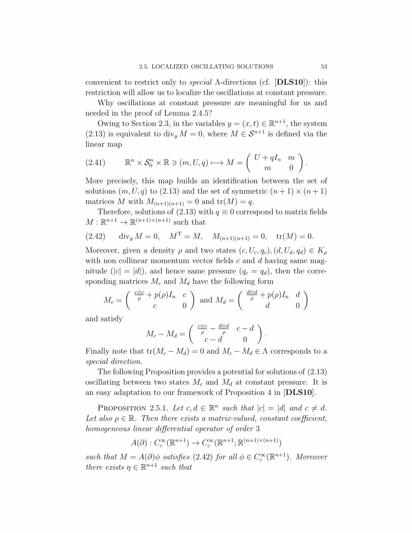
2.5. LOCALIZED OSCILLATING SOLUTIONS 53
convenient to restrict only to special Λ-directions (cf. [DLS10]): this
restriction will allow us to localize the oscillations at constant pressure.
Why oscillations at constant pressure are meaningful for us and
needed in the proof of Lemma 2.4.5?
Owing to Section 2.3, in the variables y = (x, t) ∈ Rn+1, the system
(2.13) is equivalent to divyM = 0, where M ∈ Sn+1 is defined via the
linear map
(2.41) Rn × Sn0 × R 3 (m,U, q) 7−→M =
(U + qIn m
m 0
).
More precisely, this map builds an identification between the set of
solutions (m,U, q) to (2.13) and the set of symmetric (n+ 1)× (n+ 1)
matrices M with M(n+1)(n+1) = 0 and tr(M) = q.
Therefore, solutions of (2.13) with q ≡ 0 correspond to matrix fields
M : Rn+1 → R(n+1)×(n+1) such that
(2.42) divyM = 0, MT = M, M(n+1)(n+1) = 0, tr(M) = 0.
Moreover, given a density ρ and two states (c, Uc, qc), (d, Ud, qd) ∈ Kρ
with non collinear momentum vector fields c and d having same mag-
nitude (|c| = |d|), and hence same pressure (qc = qd), then the corre-
sponding matrices Mc and Md have the following form
Mc =
(c⊗cρ
+ p(ρ)In c
c 0
)and Md =
(d⊗dρ
+ p(ρ)In d
d 0
)and satisfy
Mc −Md =
(c⊗cρ− d⊗d
ρc− d
c− d 0
).
Finally note that tr(Mc −Md) = 0 and Mc −Md ∈ Λ corresponds to a
special direction.
The following Proposition provides a potential for solutions of (2.13)
oscillating between two states Mc and Md at constant pressure. It is
an easy adaptation to our framework of Proposition 4 in [DLS10].
Proposition 2.5.1. Let c, d ∈ Rn such that |c| = |d| and c 6= d.
Let also ρ ∈ R. Then there exists a matrix-valued, constant coefficient,
homogeneous linear differential operator of order 3
A(∂) : C∞c (Rn+1)→ C∞c (Rn+1;R(n+1)×(n+1))
such that M = A(∂)φ satisfies (2.42) for all φ ∈ C∞c (Rn+1). Moreover
there exists η ∈ Rn+1 such that

54 2. NON–UNIQUENESS WITH ARBITRARY DENSITY
• η is not parallel to en+1;
• if φ(y) = ψ(y · η), then
A(∂)φ(y) = (Mc −Md)ψ′′′(y · η).
We also report Lemma 7 from [DLS10]: it ensures that the oscil-
lations of the planewaves generated in proposition 2.5.1 have a certain
size in terms of an appropriate norm-type-functional.
Lemma 2.5.2. Let η ∈ Rn+1 be a vector which is not parallel to
en+1. Then for any bounded open set B ⊂ Rn
limN→∞
∫B
sin2(Nη · (x, t))dx =1
2|B|
uniformly in t ∈ R.
For the proof we refer the reader to [DLS10].
2.6. The improvement step
We are now about to prove one of the cornerstones of the costruc-
tion. Before moving forward, let us resume the plan. We have already
identified a relaxed problem by introducing subsolutions. Then, we
have proved a sort of “h-principle” (even if there is no homotopy here)
according to which, the space of subsolutions can be “reduced” to the
space of solutions or, equivalently, the typical (in Baire’s sense) subso-
lution is a solution. Once assumed that a subsolution exists, the proof
of our “h-principle” builds upon Lemma 2.4.5 combined with Baire
category arguments. Indeed, we could also prove Proposition 2.4.1 by
applying iteratively Lemma 2.4.5 and thus constructing a converging
sequence of subsolutions approaching Kρ,χ: this would correspond to
the constructive convex integration approach (see Section 1.3.1). So
two steps are left in order to conclude our argument: showing the ex-
istence of a “starting” subsolution and prove Lemma 2.4.5.
This section is devoted to the second task, the proof of Lemma
2.4.5, while in next section we will exhibit a “concrete” subsolution.
What follows will be quite technical, therefore we first would like
to recall the plan: we will add fast oscillations in allowed directions
so to let |m|2 increase in average. The proof is inspired by [DLS09]-
[DLS10].

2.6. THE IMPROVEMENT STEP 55
Proof . [Proof of Lemma 2.4.5] Let us fix the domain Ω := Q ×[0, T ]. We look for a sequence mk ⊂ X0, with associated matrix
fields Uk, which improves m in the sense of (2.39) and has the form
(2.43) (mk, Uk) = (m,U) +∑j
(mk,j, Uk,j)
where every zk,j = (mk,j, Uk,j) is compactly supported in some suitable
ball Bk,j(xk,j, tk,j) ⊂ Ω. We proceed as follows.
Step 1. Let m ∈ X0 with associated matrix field U . By Lemma
2.3.5, for any (x, t) ∈ Ω we can find a line segment σ(x,t) := [(m(x, t), U(x, t), q0(x))−λ(x,t), (m(x, t), U(x, t), q0(x)) + λ(x,t)] admissible for (ρ0(x), χ(t)) and
with direction
λ(x,t) = (m(x, t), U(x, t), 0)
such that
(2.44) |m(x, t)| ≥ F√ρ0(x)χ(t)
(ρ0(x)χ(t)− |m(x, t)|2
).
Since z := (m,U) and Kcoρ0,χ
are uniformly continuous in (x, t), there
exists an ε > 0 such that for any (x, t), (x0, t0) ∈ Ω with |x− x0| +|t− t0| < ε, we have
(2.45) (z(x, t), q0(x))± (m(x0, t0), U(x0, t0), 0) ⊂ hintKcoρ0,χ
.
Step 2. Fix (x0, t0) ∈ Ω for the moment. Now, let 0 ≤ φr0 ≤ 1
be a smooth cutoff function on Ω with support contained in a ball
Br0(x0, t0) ⊂ Ω for some r0 > 0, identically 1 on Br0/2(x0, t0) and
strictly less than 1 outside. Thanks to Proposition 2.5.1 and the iden-
tification (m,U, q)→M , for the admissible line segment σ(x0,t0), there
exist an operator A0 and a direction η0 ∈ Rn+1 not parallel to en+1,
such that for any k ∈ N
A0
(cos(kη0 · (x, t))
k3
)= λ(x0,t0) sin(kη0 · (x, t)),
and such that the pair (mk,0, Uk,0) defined by
(mk,0, Uk,0)(x, t) := A0
[φr0(x, t)k
−3 cos(kη0 · (x, t))]

56 2. NON–UNIQUENESS WITH ARBITRARY DENSITY
satisfies (2.13) with q ≡ 0. Note that (mk,0, Uk,0) is supported in the
ball Br0(x0, t0) and that∥∥∥(mk,0, Uk,0)− φr0(m(x0, t0), U(x0, t0)
)sin(kη0 · (x, t))
∥∥∥∞
≤ const (A0, η0, ‖φ0‖C3)1
k(2.46)
since A0 is a linear differential operator of homogeneous degree 3. Fur-
thermore, for all (x, t) ∈ Br0/2(x0, t0), we have
|mk,0(x, t)|2 = |m(x0, t0)|2 sin2(kη0 · (x, t)).
Since η0 ∈ Rn+1 is not parallel to en+1, from Lemma 2.5.2 we can see
that
limk→∞
∫Br0/2
(x0,t0)
|mk,0(x, t)|2 dx =1
2
∫Br0/2
(x0,t0)
|m(x0, t0)|2 dx
uniformly in t. In particular, using (2.44), we obtain
limk→∞
∫Br0/2
(x0,t0)
|mk,0(x, t)|2 dxdt ≥
F 2
2ρ0(x0)χ(t0)
(ρ0(x0)χ(t0))− |m(x0, t0)|2
)2 ∣∣Br0/2(x0, t0)∣∣ .(2.47)
Step 3. Next, observe that since m is uniformly continuous, there
exists an r > 0 such that for any r < r there exists a finite family of
pairwise disjoint balls Brj(xj, tj) ⊂ Ω with rj < r such that∫Ω
(ρ0(x)χ(t)− |m(x, t)|2
)2dxdt ≤
2∑j
(ρ0(xj)χ(tj)− |m(xj, tj)|2
)2 ∣∣Brj(xj, tj)∣∣ .(2.48)
Fix s > 0 with s < minr, ε and choose a finite family of pairwise
disjoint balls Brj(xj, tj) ⊂ Ω with radii rj < s such that (2.48) holds.
In each ball B2rj(xj, tj) we apply the construction of Step 2 to obtain,
for every k ∈ N, a pair (mk,j, Uk,j).
Final step. Letting (mk, Uk) be as in (2.43), we observe that the
sum therein consists of finitely many terms. Therefore from (2.45) and
(2.46) we deduce that there exists k0 ∈ N such that
(2.49) mk ∈ X0 for all k ≥ k0.

2.7. CONSTRUCTION OF SUITABLE INITIAL DATA 57
Moreover, owing to (2.47) and (2.48) we can write
limk→∞
∫Ω
|mk(x, t)−m(x, t)|2 dxdt = limk→∞
∑j
∫Ω
|mk,j(x, t)|2 dxdt
≥∑j
F 2
2ρ0(xj)χ(tj)
(ρ0(xj)χ(tj))− |m(xj, tj)|2
)2 ∣∣Brj(xj, tj)∣∣
≥ C
∫Ω
(ρ0(x)χ(t)− |m(x, t)|2
)2dxdt.(2.50)
Since mkd→ m, due to (2.50) we have
lim infk→∞
‖mk‖2L2(Ω) = ‖m‖2
2 + lim infk→∞
‖mk −m‖22
≥ ‖m‖22 + C
∫Ω
(ρ0(x)χ(t)− |m(x, t)|2
)2dxdt,(2.51)
which gives (2.39) with β = β(n) = β(F (n)).
2.7. Construction of suitable initial data
In this section we show the existence of a subsolution in the sense
of Definition 3.4.1. Since the subsolution we aim to construct has to
be space-periodic, it will be enough to work on the building brick Q
and then extend the costruction periodically to Rn.
The idea to work in the space-periodic setting has been recently
adopted by Wiedemann [Wie11] in order to construct global solutions
to the incompressible Euler equations, i.e. to prove Theorem 1.3.9.
Proposition 2.7.1. Let ρ0 ∈ C1p(Q;R+) be a given density function
as in Proposition 2.4.1 and let T be any given positive time. Then, there
exist a smooth function χ : R→ R+, a continuous periodic matrix field
U : Rn → Sn0 and a function q ∈ C1(R;C1p(Rn)) such that
(2.52) divx U +∇xq = 0 on Rn × R
and
e(ρ0(x), 0, U(x)) <χ(t)
nfor all (x, t) ∈ Rn × [0, T [(2.53)
q(x, t) = p(ρ0(x)) +χ(t)
nfor all x ∈ Rn × R.(2.54)
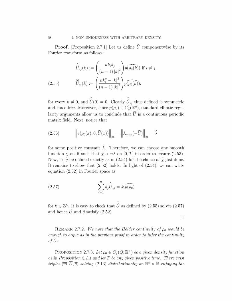
58 2. NON–UNIQUENESS WITH ARBITRARY DENSITY
Proof . [Proposition 2.7.1] Let us define U componentwise by its
Fourier transform as follows:
U ij(k) :=
(nkikj
(n− 1) |k|2
)p(ρ0(k)) if i 6= j,
U ii(k) :=
(nk2
i − |k|2
(n− 1) |k|2
)p(ρ0(k)).(2.55)
for every k 6= 0, andU(0) = 0. Clearly
U ij thus defined is symmetric
and trace-free. Moreover, since p(ρ0) ∈ C1p(Rn), standard elliptic regu-
larity arguments allow us to conclude that U is a continuous periodic
matrix field. Next, notice that
(2.56)∥∥∥e(ρ0(x), 0, U(x))
∥∥∥∞
=∥∥∥λmax(−U)
∥∥∥∞
= λ
for some positive constant λ. Therefore, we can choose any smooth
function χ on R such that χ > nλ on [0, T ] in order to ensure (2.53).
Now, let q be defined exactly as in (2.54) for the choice of χ just done.
It remains to show that (2.52) holds. In light of (2.54), we can write
equation (2.52) in Fourier space as
(2.57)n∑j=1
kjU ij = kip(ρ0)
for k ∈ Zn. It is easy to check thatU as defined by (2.55) solves (2.57)
and hence U and q satisfy (2.52)
Remark 2.7.2. We note that the Holder continuity of ρ0 would be
enough to argue as in the previous proof in order to infer the continuity
of U .
Proposition 2.7.3. Let ρ0 ∈ C1p(Q;R+) be a given density function
as in Proposition 2.4.1 and let T be any given positive time. There exist
triples (m,U, q) solving (2.13) distributionally on Rn ×R enjoying the
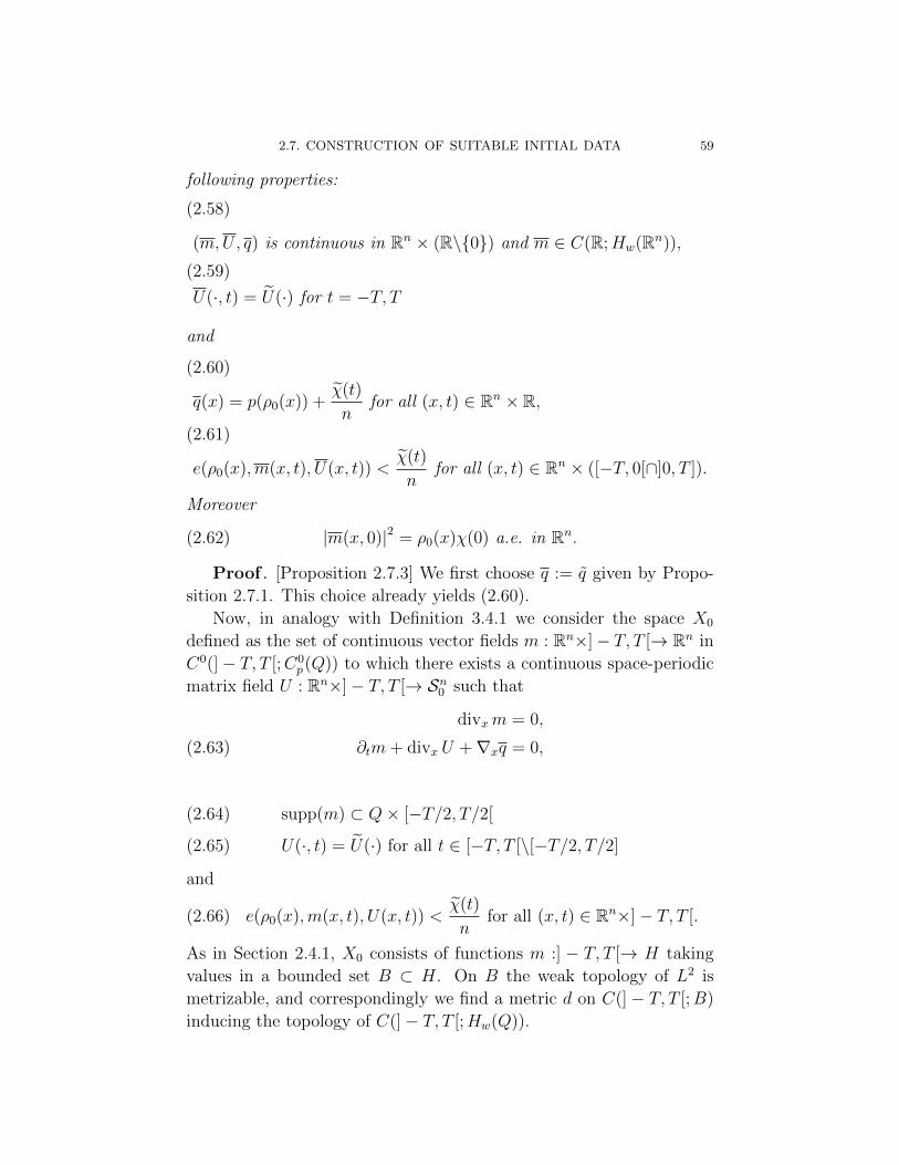
2.7. CONSTRUCTION OF SUITABLE INITIAL DATA 59
following properties:
(m,U, q) is continuous in Rn × (R\0) and m ∈ C(R;Hw(Rn)),
(2.58)
U(·, t) = U(·) for t = −T, T(2.59)
and
q(x) = p(ρ0(x)) +χ(t)
nfor all (x, t) ∈ Rn × R,
(2.60)
e(ρ0(x),m(x, t), U(x, t)) <χ(t)
nfor all (x, t) ∈ Rn × ([−T, 0[∩]0, T ]).
(2.61)
Moreover
(2.62) |m(x, 0)|2 = ρ0(x)χ(0) a.e. in Rn.
Proof . [Proposition 2.7.3] We first choose q := q given by Propo-
sition 2.7.1. This choice already yields (2.60).
Now, in analogy with Definition 3.4.1 we consider the space X0
defined as the set of continuous vector fields m : Rn×]− T, T [→ Rn in
C0(]− T, T [;C0p(Q)) to which there exists a continuous space-periodic
matrix field U : Rn×]− T, T [→ Sn0 such that
divxm = 0,
∂tm+ divx U +∇xq = 0,(2.63)
supp(m) ⊂ Q× [−T/2, T/2[(2.64)
U(·, t) = U(·) for all t ∈ [−T, T [\[−T/2, T/2](2.65)
and
(2.66) e(ρ0(x),m(x, t), U(x, t)) <χ(t)
nfor all (x, t) ∈ Rn×]− T, T [.
As in Section 2.4.1, X0 consists of functions m :] − T, T [→ H taking
values in a bounded set B ⊂ H. On B the weak topology of L2 is
metrizable, and correspondingly we find a metric d on C(]− T, T [;B)
inducing the topology of C(]− T, T [;Hw(Q)).

60 2. NON–UNIQUENESS WITH ARBITRARY DENSITY
Next we note that with minor modifications the proof of Lemma
2.4.5 leads to the following claim:
Claim: Let Q0 ⊂ Q be given. Let m ∈ X0 with associated matrix
field U and let α > 0 such that∫Q0
[|m(x, 0)|2 − (ρ0(x)χ(0))
]dx < −α
Then, for any δ > 0 there exists a sequence mk ∈ X0 with associated
smooth matrix field Uk such that
supp(mk −m,Uk − U) ⊂ Q0 × [−δ, δ],
mkd→ m,
and
lim infk→∞
∫Q0
|mk(x, 0)|2 ≥∫Q0
|m(x, 0)|2 dx+ βα2.
Fix an exhausting sequence of bounded open subsets Qk ⊂ Qk+1 ⊂Q, each compactly contained in Ω, and such that |Qk+1\Qk| ≤ 2−k.
Let also γε be a standard mollifying kernel in Rn (the unusual notation
γε for the standard mollifying kernel is aimed at avoiding confusion be-
tween it and the density function). Using the claim above we construct
inductively a sequence of momentum vector fields mk ∈ X0, associated
matrix fields Uk and a sequence of numbers ηk < 2−k as follows.
First of all let m1 ≡ 0, U1(x, t) = U(x) for all (x, t) ∈ Rn+1 and
having obtained (m1, U1), ..., (mk, Uk), η1, ..., ηk−1 we choose ηk < 2−k
in such a way that
(2.67) ‖mk −mk ∗ γηk‖L2 < 2−k.
Then, we set
αk = −∫Qk
[|mk(x, 0)|2 − ρ0(x)χ(0))]dx.
Note that (2.66) ensures αk > 0. Then, we apply the claim with
Qk, α = αk and δ = 2−kT to obtain mk+1 ∈ X0 and associated smooth
matrix field Uk+1 such that
(2.68) supp(mk+1 −mk, Uk+1 − Uk) ⊂ Qk × [−2−kT, 2−kT ],
(2.69) d(mk+1,mk) < 2−k,
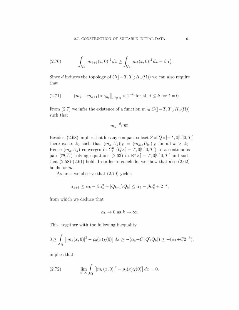
2.7. CONSTRUCTION OF SUITABLE INITIAL DATA 61
(2.70)
∫Qk
|mk+1(x, 0)|2 dx ≥∫Qk
|mk(x, 0)|2 dx+ βα2k.
Since d induces the topology of C(]−T, T [;Hw(Ω)) we can also require
that
(2.71)∥∥(mk −mk+1) ∗ γηj
∥∥L2(Ω)
< 2−k for all j ≤ k for t = 0.
From (2.7) we infer the existence of a function m ∈ C(]−T, T [, Hw(Ω))
such that
mkd→ m.
Besides, (2.68) implies that for any compact subset S ofQ×]−T, 0[∪]0, T [
there exists k0 such that (mk, Uk)|S = (mk0 , Uk0)|S for all k > k0.
Hence (mk, Uk) converges in C0loc(Q×] − T, 0[∪]0, T [) to a continuous
pair (m,U) solving equations (2.63) in Rn×] − T, 0[∪]0, T [ and such
that (2.58)-(2.61) hold. In order to conclude, we show that also (2.62)
holds for m.
As first, we observe that (2.70) yields
αk+1 ≤ αk − βα2k + |Qk+1\Qk| ≤ αk − βα2
k + 2−k,
from which we deduce that
αk → 0 as k →∞.
This, together with the following inequality
0 ≥∫Q
[|mk(x, 0)|2 − ρ0(x)χ(0)
]dx ≥ −(αk+C |Q\Qk|) ≥ −(αk+C2−k),
implies that
(2.72) limk↑∞
∫Ω
[|mk(x, 0)|2 − ρ0(x)χ(0)
]dx = 0.

62 2. NON–UNIQUENESS WITH ARBITRARY DENSITY
On the other hand, owing to (2.67) and (2.71), we can write for t = 0
and for every k
‖mk −m‖L2
≤ ‖mk −mk ∗ γηk‖L2 + ‖mk ∗ γηk −m ∗ γηk‖L2 + ‖m ∗ γηk −m‖L2
≤ 2−k +∞∑j=0
‖mk+j ∗ γηk −mk+j+1 ∗ γηk‖L2 + 2−k
≤ 2−(k−2).
(2.73)
Finally, (2.73) implies that mk(·, 0) → m(·, 0) strongly in H(Q) as
k →∞, which together with (2.72) gives
|m(x, 0)|2 = ρ0(x)χ(0) for almost every x ∈ Rn.
2.8. Proof of the main Theorems
Proof . [Proof of Theorem 2.2.1] Let T be any finite positive time
and ρ0 ∈ C1p(Q) be a given density function. Let also (m,U, q) be as
in Proposition 2.7.3. Then, define χ(t) := χ(t), q0(x) := q(x),
(2.74) m0(x, t) =
m(x, t) for t ∈ [0, T ]
m(x, t− 2T ) for t ∈ [T, 2T ],
(2.75) U0(x, t) =
U(x, t) for t ∈ [0, T ]
U(x, t− 2T ) for t ∈ [T, 2T ].
For this choices, the quadruple (m0, U0, q0, χ) satisfies the assump-
tions of Proposition 2.4.1. Therefore, there exist infinitely many solu-
tions m ∈ C([0, 2T ], Hw(Q)) of (2.8) in Rn × [0, 2T [ with density ρ0,
such that
m(x, 0) = m(x, 0) = m(x, 2T ) for a.e. x ∈ Ω
and
(2.76) |m(·, t)|2 = ρ0(·)χ(0) for almost every (x, t) ∈ Rn×]0, 2T [.
Since |m0(·, 0)|2 = ρ0(·)χ(0) a.e. in Rn as well, it is enough to define
m0(x) = m0(x, 0) to satisfy also (2.12) and hence conclude the proof.

2.8. PROOF OF THE MAIN THEOREMS 63
Proof . [Proof of Theorem 2.2.2] Under the assumptions of Theo-
rem 2.2.1, we have proven the existence of a bounded initial momentum
m0 allowing for infinitely many solutions m ∈ C([0, T ];Hw(Q)) of (2.8)
on Rn×[0, T [ with density ρ0. Moreover, the proof (see Proof of Propo-
sition 2.7.1) showed that for any smooth function χ : R → R+ with
χ > nλ > 0 the following holds
|m(x, t)|2 = ρ0(x)χ(t) a.e. in Rn × [0, T [,(2.77) ∣∣m0(x)∣∣2 = ρ0(x)χ(0) a.e. in Rn.(2.78)
Now, we claim that there exist constants C1, C2 > 0 such that choos-
ing the function χ(t) > nλ on [0, T [ among solutions of the following
differential inequality
(2.79) χ′(t) ≤ −C1χ1/2(t)− C2χ
3/2(t),
then the weak solutions (ρ0,m) of (2.8) obtained in Theorem 2.2.1 will
also satisfy the admissibility condition (3.26) on Rn× [0, T [. Of course,
there is an issue of compatibility between the differential inequality
(2.79) and the condition χ > nλ: this motivates the existence of a time
T > 0 defining the maximal time-interval in which the admissibility
condition indeed holds.
Let T be any finite positive time. As first, we aim to prove the claim.
Since m ∈ C([0, T ];Hw(Q)) is divergence-free and fulfills (2.77)-(2.78)
and ρ0 is time-independent, (3.26) reduces to the following inequality
(2.80)1
2χ′(t)+m ·∇
(ε(ρ0(x))+
p(ρ0(x))
ρ0(x)
)+χ(t)
2m ·∇
(1
ρ0(x)
)≤ 0,
intended in the sense of (space-periodic) distributions on Rn × [0, T ].
As ρ0 ∈ C1p(Q), there exists a constant c2
0 with ρ0 ≤ c20 on Rn, whence
(see (2.77)-(2.78) )
(2.81) |m(x, t)| ≤ c0
√χ(t) a.e. on Rn × [0, T [.
Similarly we can find constants c1, c2 > 0 with∣∣∣∣∣∇(ε(ρ0(x)) +
p(ρ0(x))
ρ0(x)
)∣∣∣∣∣ ≤ c1 a.e. in Rn(2.82) ∣∣∣∣∇( 1
ρ0(x)
)∣∣∣∣ ≤ c2 a.e. in Rn.(2.83)

64 2. NON–UNIQUENESS WITH ARBITRARY DENSITY
As a conseguence of (2.81)-(2.83), (2.80) holds as soon as χ satisfies
χ′(t) ≤ −2c1c0χ1/2(t)− c2c0χ
3/2(t) on [0, T [.
Therefore, by choosing C1 := 2c1c0 and C2 := c2c0 we can conclude the
proof of the claim.
Now, it remains to show the existence of a function χ as in the
claim, i.e. that both the differential inequality (2.79) and the condition
χ > nλ can hold true on some suitable time-interval. To this aim, we
can consider the equality in (2.79), couple it with the initial condition
χ(0) = χ0 for some constant χ0 > nλ and then solve the resulting
Cauchy problem. For the obtained solution χ, there exists a positive
time T such that χ(t) > nλ on [0, T [.
Finally, applying the claim on the time-interval [0, T [ we conclude
that the admissibility condition holds on Rn × [0, T [ as desired.
Proof . [Proof of Theorem 2.1.1] The proof of Theorem 2.1.1 strongly
relies on Theorems 2.2.1-2.2.2. Given a continuously differentiable ini-
tial density ρ0 we apply Theorems 2.2.1-2.2.2 for ρ0(x) := ρ0(x) thus
obtaining a positive time T and a bounded initial momentum m0 al-
lowing for infinitely many solutions m ∈ C([0, T ];Hw(Q)) of (2.8) on
Rn × [0, T [ with density ρ0 and such that the following holds
|m(x, t)|2 = ρ0(x)χ(t) a.e. in Rn × [0, T [,(2.84) ∣∣m0(x)∣∣2 = ρ0(x)χ(0) a.e. in Rn,(2.85)
for a suitable smooth function χ : [0, T ] → R+. Now, define ρ(x, t) =
ρ0(x)1[0,T [(t). This shows that (3.25) holds. To prove (3.24) observe
that ρ is independent of t and m is weakly divergence-free for almost
every 0 < t < T . Therefore, the pair (ρ,m) is a weak solution of
(2.1) with initial data (ρ0,m0). Finally, we can also prove (3.26): each
solution obtained is also admissible. Indeed, for ρ(x, t) = ρ0(x)1[0,T [(t),
(3.26) is ensured by Theorem 2.2.2.

CHAPTER 3
Non–standard solutions to the compressible Euler
equations with Riemann data
3.1. Introduction
In this chapter, we will focus on the Cauchy problem for the isen-
tropic compressible Euler equations of gas dynamics in two space space
dimensions: we will consider Riemann data having a specific form and
we will prove the following surprising result which corresponds to The-
orem 0.2.2 in the Introduction of the thesis.
Theorem 3.1.1. For some choices of the pressure law p with p′ > 0
(among which p(ρ) = ρ2) and for some specific Riemann initial data,
there exist infinitely many bounded entropy solutions of the isentropic
compressible Euler equations in two space dimensions, all with density
bounded away from zero.
The proof builds upon the methods of [DLS09]-[DLS10] where
De Lellis and Szekelyhidi had already shown that the admissibility
(entropy) condition does not imply uniqueness of L∞ solutions of the
Cauchy problem and upon the developments achieved in [Chi11] and
illustrated in Chapter 2. However, the examples in the papers [DLS10]
and [Chi11] had very rough initial data and it was not at all clear
whether more regular data could be achieved.
The previous result was inspired by the recent work of Szekelyhidi,
who in [Sz1] recasts the vortex-sheet problem of incompressible fluid
dynamics in the framework of [DLS11].
We therefore chose to review the construction of Szekelyhidi in [Sz1]
in next section (Section 3.2) before illustrating the new ideas and strate-
gies devised to prove Theorem 3.1.1.
The rest of the chapter is organized as follows. In Section 3.3 we
give the precise statement of Theorem 3.1.1 by describing the form of
the initial data allowing for such a result and by characterizing the set
65
66 3. COMPRESSIBLE EULER EQUATIONS WITH RIEMANN DATA
of allowed pressure laws. In Section 3.4 we overview the basic defini-
tions and the main ingredients of our setting. Section 3.5 explains how
the convex integration approach introduced by De Lellis-Szekelyhidi
applies to our framework and allows us to prove Theorem 3.1.1. Sec-
tion 3.6 and 3.7 are devoted to the final argument for the proof of
Theorem 3.1.1: the construction of a subsolution.
3.2. Weak solutions to the incompressible Euler equations
with vortex sheet initial data
Recently Szekelyhidi constructed infinitely many admissible weak
solutions to the incompressible Euler equations with initial data given
by the classical vortex sheet. He considered the Cauchy problem for
the incompressible Euler equations (see Section 1.3.2),
(3.1)
divxv = 0
∂tv + divx (v ⊗ v) +∇xp = 0
v(·, 0) = v0
.
where the unknowns v and p are the velocity vector and the pressure.
His construction is based on the “convex integration” method intro-
duced recently in [DLS10]. His result inspired us and in particular
suggested that a similar approach could be of interest also for the com-
pressible Euler system thus leading to Theorem 3.1.1.
The starting point of Szekelyhidi’s construction lies in the approach
of [DLS09]-[DLS10] towards the construction of weak solutions to the
incompressible Euler equations (3.1) in order to recover the celebrated
non–uniqueness results of Scheffer [Sch93] and Shnirelman [Shn97]
(see Section 1.3.2.1). The method in [DLS09]-[DLS10] is a revisita-
tion of convex integration and Baire category arguments. In particu-
lar, in [DLS10] the strategy behind the construction of “admissible”
weak solutions to the initial value problem was based on the notion of
subsolution. Thanks to this strategy, in [DLS10] it was shown that
admissibility by itself does not imply uniqueness for the incompress-
ible Euler system (3.1). In other words there exist initial data v0, for
which there exist infinitely many distinct admissible weak solutions of
the incompressible Euler equations (3.1). Such initial data are called
wild initial data in [DLS10]. In particular, one can show the exis-
tence of infinitely many weak solutions satisfying the Duchon-Robert

3.2. WILD VORTEX SHEET 67
admissibility condition (see section 1.3.2)
(3.2) ∂t|v|2
2+ div
((|v|2
2+ p
)v
)≤ 0.
Obviously, wild initial data have to possess a certain amount of ir-
regularity. This follows from the weak- strong uniqueness and classical
local existence results. From the construction of wild initial data in
[DLS10] it was not clear how bad this irregularity needs to be. In
[Sz1] Szekelyhidi showed that the classical vortex-sheet with a flat in-
terface is a wild initial data. More precisely, consider the following
solenoidal vector field in R2
(3.3) v0(x) :=
v+ := (1, 0) if x2 > 0,
v− := (−1, 0) if x2 < 0,
then the following theorem holds:
Theorem 3.2.1 (The vortex sheet is wild). For v0 as in (3.3) there
are infinitely many weak solutions of (3.1) on R2× [0,∞) which satisfy
the admissibility condition (3.2).
As already explained in section 1.3.2, Theorem 3.2.1 is proved in
[Sz1] using an adapted version of Proposition 1.3.5: hence the proof
essentially consisted in finding a suitable subsolution for the incom-
pressible Euler system which takes the right initial values. For the
sake of completeness, we recall the relevant definitions and results in
the case of two space-dimensions:
Definition 3.2.2 (Incompressible subsolutions). A subsolution to
the incompressible Euler equations with respect to the kinetic energy e
is a triple (v, u, q) : R2×]0,∞[→ (R2,S2×20 ,R+) with v ∈ L2
loc, u ∈ L1loc,
q ∈ D′ and such that
(3.4)
∂tv + divxu+∇xq = 0
divxv = 0
in the sense of distributions and
(3.5) v ⊗ v − u ≤ eId a.e..
Proposition 1.3.5 is here recasted as follows:
Theorem 3.2.3 (Proposition 2 in [DLS10]). Let (v, u, q) be a sub-
solution to the incompressible Euler equations on R2×]0, T [. Assume
68 3. COMPRESSIBLE EULER EQUATIONS WITH RIEMANN DATA
that W ⊂ R2×]0, T [ is an open set such that (v, u, q) are continuous
on W and
(3.6) v ⊗ v − u < eId on W .
Then, there exist infinitely many (v, u) ∈ L∞loc(R2×R) with v ∈ C(R;L2w(R2))
such that (v, u, 0) satisfies (3.4), (v, u) = 0 a.e. on Wc, and
(3.7) (v + v)⊗ (v + v)− (u+ u) = eId a.e. in W .
In particular, if v := v + v in the above theorem, then v satisfies
the incompressible Euler equations in the space-time region W with
pressure q, where
(3.8) |v|2 = 2e, q = q − e.
In other words, if the subsolution is a continuous, strict subsolution in
some subregion, then it is possible (in a highly non-unique way) to add
a perturbation so that the sum is a solution of the incompressible Euler
equations (3.1) with prescribed kinetic energy density. This theorem
is essentially the content of Proposition 2 in [DLS10] with an almost
identical proof, except that in the proof one needs to perform the cov-
ering inside the region W rather than in all of space-time. Theorem
3.2.3 leads to the following criterion for the initial datum (3.3) to be a
wild datum. In what follows we will work in the simple case of e = 12.
Theorem 3.2.4. Let v0 be as in (3.3). Assume that there exists a
subsolution (v, u, q) for the incompressible Euler equations with
(3.9) v ∈ C([0, T ];L2w(R2)), v(0) = v0.
Furthermore, assume that there exists an open set W ⊂ R2×]0, T [ such
that (v, u, q) is continuous on W and
v ⊗ v − u < 1
2Id in W .(3.10)
v ⊗ v − u =1
2Id a.e. in Wc.(3.11)
Then, there exist infinitely many weak solutions to the incompressible
Euler equations on R2×]0, T [ satisfying (3.2) and with initial data v0.
In [Sz1] the construction of a subsolution as required by Theo-
rem 3.2.4 follows an idea introduced in [Sze11] for the incompressible
porous media equation. Here we will show that the existence of such a
3.2. WILD VORTEX SHEET 69
subsolution can be achieved also in a more direct way which will be of
use in the compressible case as well.
3.2.1. Direct proof of Theorem 3.2.1. The aim of this section
is to apply Theorem 3.2.4 in order to prove Theorem 3.2.1. Clearly
we need to find a triple (v, u, q) satisfying (3.4), (3.9) and (3.10) for
some open set W ⊂ R2×]0, T [. We will denote the space variable as
x = (x1, x2) ∈ R2. To this aim, we consider potential subsolutions of
the following form:
(v, u, q) = (v−, u−, q−)1R−
+ (v, u, q)1R
+ (v+, u+, q+)1R+ ,(3.12)
with
R− :=
0 < t <
x2
ν1
,
R :=
t >
x2
ν1
and t >x2
ν2
,
R+ :=
0 < t <
x2
ν2
and
(3.13) v = (α, 0),
(3.14) u− = u+ =
(12
0
0 −12
),
(3.15) q− = q+ =1
2,
(3.16) u =
(β γ
γ −β
),
for some constants ν1 < 0 < ν2, α, β, γ and q. Inside each of the
three regions R−, R and R+ the equations defining a subsolution are
trivially satisfied; hence they need to be imposed only along fronts
which do not depend on x1. Moreover condition (3.9) trivially holds.

70 3. COMPRESSIBLE EULER EQUATIONS WITH RIEMANN DATA
Since the divergence free condition is trivially satisfied for our choice
of v, the system (3.4) simply reads as
ν2(α− 1) = γ,(3.17a)
β = q,(3.17b)
ν1(α + 1) = γ.(3.17c)
Finally, if we chooseW to coincide with R, then the requirement (3.10)
amounts to the condition
(3.18)
(α2 − β −γ−γ β
)<
(12
0
0 12
),
which is equivalent to the following couple of inequalities
α2 ≤ 1,(3.19a)
1
4− 1
2α2 + βα2 − β2 − γ2 ≥ 0.(3.19b)
With the choice α = 0, ν1 = −ν2 = γ < 0 and −γ = β = q = 14. all
the conditions (3.17a)-(3.19b) are satisfied. Hence a subsolution as in
the hypothesis of Theorem 3.5.1 exists. Note that for the initial datum
v0 as given by (3.3) we already have: |v0|2 = 2e = 1 for our choice
of e. This together with the fact the pressure does not depend on x1
(since q and e = 12
do not depend on x1) justifies why the admissibility
condition (3.2) will be satisfied by the so constructed infinitely many
weak solutions of the incompressible Euler equations.
3.3. The compressible system: main results
The motivation to the results herein presented has already been dis-
closed in the Introduction to the chapter. We emphasize that [DLS10]
inspired the construction carried out in Chapter 2 (see also [Chi11]),
where the compressible Euler equations are analyzed in the framework
of convex integration: by choosing a suitable concept of subsolution, a
similar strategy as in [DLS09, DLS10] can be performed and failure of
uniqueness of admissible weak solutions to the Cauchy problem for the
compressible Euler equations starting from any regular initial density
is shown. This further result confirms the conjecture that admissi-
bility by itself does not imply uniqueness for the compressible Euler
equations and highlights the main role of the velocity in this failure
of uniqueness. As for the incompressible Euler equations, there exist

3.3. THE COMPRESSIBLE SYSTEM: MAIN RESULTS 71
initial data with infinitely many distinct admissible weak solutions of
the compressible Euler equations. These initial data can be denomi-
nated as wild initial data, coherently with the incompressible case. As
explained in Chapter 2, wild initial data need to be irregular : if the
initial data are smooth enough, then a classical weak solution exists on
a maximal time interval and is unique within the broader class of weak
solutions (cf. [Daf00]).
A natural question then arises: how bad does this irregularity needs
to be? Here we give a partial answer to this question: we show that
a classical Riemann initial datum is a wild initial datum in the two
dimensional case. More precisely, we consider the Cauchy problem
for the compressible Euler equations in two space dimensions and we
exhibit a Riemann initial datum allowing for infinitely many admissible
weak solutions.
We recall once more in the thesis, for the first time in this chapter,
the isentropic compressible Euler equations of gas dynamics in two
space dimensions. The unknowns of the equations are the density ρ and
the velocity v (see (0.1)). The Cauchy problem for the compressible
Euler system, which consists of 3 scalar equations in the two-space-
dimensional case, takes the form:
(3.20)
∂tρ+ divx(ρv) = 0
∂t(ρv) + divx (ρv ⊗ v) +∇x[p(ρ)] = 0
ρ(·, 0) = ρ0
v(·, 0) = v0
.
The pressure p is a function of ρ whose analytical form depends on the
gas under investigation. A common choice is the polytropic pressure
law
p(ρ) = kργ
with constants k > 0 and γ > 1. The first main result will be concerned
with the case p(ρ) = kρ2. This choice is consistent with classical kinetic
theory which predicts γ = 1 + 2/d where d is the number of degrees
of freedom: indeed in the two space-dimensional case we have exactly
d = 2 hence the chosen value of γ.

72 3. COMPRESSIBLE EULER EQUATIONS WITH RIEMANN DATA
Entropy or admissible solutions are those satisfying an additional
constraint (also called entropy inequality) coming from the energy in-
equality
(3.21) ∂t
(ρε(ρ) + ρ
|v|2
2
)+ divx
[(ρε(ρ) + ρ
|v|2
2+ p(ρ)
)v
]≤ 0
where the internal energy ε : R+ → R is given through the law p(r) =
r2ε′(r).
If we consider Riemann data ρ0 and v0 having the following very specific
form
(3.22) ρ0(x) :=
ρ+ if x2 > 0,
ρ− if x2 < 0,
(3.23) v0(x) :=
v+ := (1, 0) if x2 > 0,
v− := (−1, 0) if x2 < 0,
then the following theorems hold (precise statements of Theorem 3.1.1).
Theorem 3.3.1. With the choice of pressure law p(ρ) = ρ2, there
exist constants ρ± for which there exist infinitely many admissible bounded
solutions (ρ, v) of (3.20), (3.22)-(3.23) with inf ρ > 0.
Theorem 3.3.2. For some specific smooth pressure laws p with
p′ > 0, there exist constants ρ± for which there exist infinitely many
admissible bounded solutions (ρ, v) of (3.20), (3.22)-(3.23) with inf ρ >
0.
If we restrict our attention to pairs (ρ, v) which are admissible so-
lutions of (3.20), (3.22)-(3.23) and depend only on (x2, t), then we
will be dealing with a classical Riemann problem for (3.20) in one
space-variable (only x2) which admits self-similar solutions. Since the
pioneering work of Riemann it is known that, under the hypothesis
of “self-similarity” of (ρ, v) (dependence only on x2t
) and with some
other assumptions, there is a unique solution of (3.20), (3.22)-(3.23)
(see for instance [Ser99]). We will show that, such a uniqueness result
holds also for the choice of pressure law dictated by Theorem 3.3.1:
this will be the content of next chapter. But Theorems 3.3.1 and 3.3.2
show that uniqueness is completely lost if we drop the requirement that
(ρ, v) depends only on x2t
.
3.4. BASIC DEFINITIONS 73
Moreover, Theorems 3.3.1 and 3.3.2 deserve some further com-
ments. The pressure laws p which allow our constructions are not
a condition sine qua non for the non-uniqueness results to hold. An
interesting question correlated to our result is whether Theorem 3.3.2
might hold for regular initial data: so far the problem is open since the
data of Theorem 3.3.2 cannot be generated by Lipschitz compression
waves.
Finally, though the solutions of Theorems 3.3.1 and 3.3.2 are very
irregular, it is rather unclear where one wishes to set a boundary. On
the one hand the space of BV functions does not seem suitable for an
existence theory in more than one space dimension (see [Rau86]). On
the other hand the recent paper [DLS12] shows the existence of con-
tinuous solutions to the incompressible Euler equations which dissipate
the kinetic energy. This may suggest that the framework of [DLS09]-
[DLS10] is likely to produce “strange” piecewise continuous solutions
to hyperbolic systems of conservation laws.
3.4. Basic definitions
Let T be a fixed positive time. By a weak solution of (3.20) on
R2 × [0, T [ we mean a pair (ρ, v) ∈ L∞(R2 × [0, T [) such that the
following identities hold for every test functions ψ ∈ C∞c (R2 × [0, T [),
φ ∈ C∞c (R2 × [0, T [):
(3.24)
∫ T
0
∫R2
[ρ∂tψ + ρv · ∇xψ] dxdt+
∫R2
ρ0(x)ψ(x, 0)dx = 0
∫ T
0
∫R2
[ρv · ∂tφ+ 〈ρv ⊗ v,∇xφ〉+ p(ρ) divx φ] dxdt
+
∫R2
ρ0(x)v0(x) · φ(x, 0)dx = 0.(3.25)
For n = 2 the only non-trivial entropy is the total energy η =
ρε(ρ) + ρ|v|22
which corresponds to the flux Ψ =(ε(ρ) + ρ |v|
2
2+ p(ρ)
ρ
)v.

74 3. COMPRESSIBLE EULER EQUATIONS WITH RIEMANN DATA
Then a bounded weak solution (ρ, v) of (3.20) satisfying (3.21) in
the sense of distributions, i.e. satisfying the following inequality∫ T
0
∫R2
[(ρε(ρ) + ρ
|v|2
2
)∂tϕ+
(ρε(ρ) + ρ
|v|2
2+ p(ρ)
)v · ∇xϕ
]
+
∫R2
(ρ0ε(ρ0) + ρ0 |v0|2
2
)ϕ(·, 0) ≥ 0,
(3.26)
for every nonnegative ϕ ∈ C∞c (R2× [0, T [), is said to be an entropy (or
admissible) solution of (3.20).
3.4.1. Subsolutions. In order to prove Theorem 3.3.2 we first
recall the underlying strategy. To start with, we make precise the
definition of subsolution in our context. Here S2×20 denotes the set of
symmetric traceless 2× 2 matrices and Id is the identity matrix.
Definition 3.4.1 (Compressible subsolutions). A subsolution to
the compressible Euler equations (3.20) is a triple (ρ, v, u) : R2×]0,∞[→(R+,R2,S2×2
0 ), with ρ ∈ L∞, v ∈ L2loc and u ∈ L1
loc, satisfying the fol-
lowing properties:
(1) (ρ, v, u) =∑N
i=1(ρi, vi, ui)1Pifor some partition P1, ..., PN of
R2×]0,∞[ in finitely many open sets and for some constants
(ρi, vi, ui);
(2) ∀ 1 ≤ i ≤ N , one of the following two conditions holds on Pi:
either
(3.27) |vi| = 1 and ui = vi ⊗ vi −|vi|2
2Id a.e.,
or
(3.28) |vi|2 < Ci and vi ⊗ vi − ui <Ci2Id a.e..
for some positive constant Ci,
and solving
(3.29)∂tρ+ divx(ρ v) = 0
∂t(ρ v) + divx (ρ u) +∇x
(p(ρ) +
∑i∈IC Ci
ρ21Pi
+∑
i∈I1ρ21Pi
)= 0
ρ(·, 0) = ρ0
v(·, 0) = v0
.

3.5. CONVEX INTEGRATION 75
in the sense of distributions, where the sets of indexes I1 and IC are
defined as follows:
I1 := i ∈ [1, N ] ∩ N such that (3.27) holds on Pi,
IC := i ∈ [1, N ] ∩ N such that (3.28) holds on Pi.
Now, we will introduce a completely new definition which will be
the starting point for the convex integration argument.
Definition 3.4.2 (Admissible subsolutions). A subsolution (ρ, v, u) :
R2×]0,∞[→ (R+,R2,S2×20 ) to the compressible Euler equations (3.20)
is said to be admissible if it satisfies the following inequality in the sense
of distributions:
∂t (ρε(ρ)) + divx [(ρε(ρ) + p(ρ)) v]
+∑i∈IC
[∂t
(ρCi − 1
21Pi
)]+∑i∈IC
[divx
(ρ v
Ci − 1
21Pi
)]≤ 0.
(3.30)
For our purposes we will also make use of “incompressible subsolu-
tions” as defined in Definition 3.2.2 with the particular choice e = C/2
for some positive constant C, i.e.:
Definition 3.4.3 (Incompressible subsolutions 2). A subsolution
to the incompressible Euler equations is a triple (v, u, q) : R2×]0,∞[→(R2,S2×2
0 ,R+) with v ∈ L2loc, u ∈ L1
loc, q ∈ D′ and such that
(3.31)
∂tv + divxu+∇xq = 0
divxv = 0
in the sense of distributions and
(3.32) v ⊗ v − u < C
2Id a.e..
Note that subsolutions to the incompressible Euler equations auto-
matically satisfy |v|2 < C a.e. If, in addition, (3.32) is an equality a.e.
then v is a weak solution of the incompressible Euler equations.
3.5. Convex integration
In this section, we will clarify how convex integration allows to
construct admissible weak solutions to the compressible Euler system
(3.20) with Riemann initial data (ρ0, v0) starting from admissible sub-
solutions. Given an admissible subsolution (ρ, v, u) for the compressible

76 3. COMPRESSIBLE EULER EQUATIONS WITH RIEMANN DATA
Euler system as in definition 3.4.1-3.4.2, the density ρ is constant in
every open set Pi of the partition; therefore, in those open sets Piwhere (3.28) holds, we are indeed dealing with a subsolution for the
incompressible Euler system in the sense of definition 3.4.3. More pre-
cisely, in the open sets Pi where (3.28) holds, the triple (vi, ui, 0) is,
by definition, a subsolution on Pi to the incompressible Euler system.
This observation suggests that, in every open set Pi where (3.28) holds,
we can exploit the results obtained in [DLS10] for the incompressible
Euler equations: in every such open set it is indeed possible to run a
suitable version of convex integration so to construct infinitely many
weak solutions. To this aim we will make use of Proposition 3.2.3 from
[DLS10] with the choice e = C/2. Theorem 3.2.3 leads to the following
criterion for wild initial data for the compressible Euler equations.
Theorem 3.5.1. Let (ρ0, v0) be as in (3.22)-(3.23). Assume that
there exists an admissible subsolution (ρ, v, u) for the compressible Eu-
ler equations with
(3.33) v(0) = v0, ρ(0) = ρ0.
Then, there exist infinitely many admissible weak solutions to the com-
pressible Euler equations on R2×]0, T [ with initial data (ρ0, v0).
Proof . Let (ρ, v, u) be an admissible subsolution for the compress-
ible Euler equations as given by the assumptions of Theorem 3.5.1.
In particular, we can assume that (ρ, v, u) =∑N
i=1(ρi, vi, ui)1Pi. For
every open set Pi where (3.28) holds, we apply Theorem 3.2.3 to the
triple (vi, ui, 0) on the open setW = Pi. Then, we find infinitely many
functions (vi, ui) satisfying (3.31) on R2×]0,∞[ with q = 0 and such
that the following holds:
(vi + vi)⊗ (vi + vi)− (ui + ui) =Ci2Id a.e. in Pi,(3.34)
(vi, ui) = 0 a.e. on P ci .(3.35)
Once Theorem 3.2.3 has been applied to every open set Pi where (3.28)
holds (i.e. for every i ∈ IC), we define v and u in a highly non-unique
way as follows:
v := v +N∑i=1
vi,

3.6. NON–STANDARD SOLUTIONS WITH QUADRATIC PRESSURE 77
u := u+N∑i=1
ui
Since ρ is constant on every Pi and thanks to (3.29), (3.30) and (3.34)-
(3.35), the infinitely many couples (ρ, v) are admissible weak solutions
of (3.20) on R2×]0, T [ with initial data (ρ0, v0).
Thanks to Theorem 3.5.1, in order to prove Theorems 3.3.1 and
3.3.2 it will be enough to exhibit an admissible subsolution to the com-
pressible Euler equations in the sense of Definition 3.4.2. The con-
struction of such a subsolution will be the content of the next sections.
At this point the chapter takes two different routes according to the
theorem we are going to prove.
3.6. Non–standard solutions with quadratic pressure
3.6.1. Construction of the subsolution. In this section, we will
prove the existence of an admissible subsolution for the quadratic pres-
sure law satisfying (3.33).
Theorem 3.6.1. For p(ρ) = ρ2 there are constants ρ± such that
there exists an admissible subsolution (ρ, v, u) : R2×]0,∞[→ (R+,R2,S2×20 )
to the compressible Euler equations with
(3.36) v(0) = v0, and ρ(0) = ρ0,
for ρ0 and v0 as in (3.22)-(3.23).
Remark 3.6.2. The admissible subsolution of Theorem 3.6.1 will
have the form
(ρ, v, u) =3∑i=1
(ρi, vi, ui)1Pi,
for some suitably chosen Pi, 1 ≤ i ≤ 3.
What follows is devoted to the proof of Theorem 3.6.1.
3.6.1.1. Subsolutions in three regions. We aim at constructing an
admissible subsolution to the compressible Euler equations of the fol-
lowing form (see Fig. 1):
(ρ, v, u) = (ρ−, v−, u−)1P−
+ (ρ, v, u)1P
+ (ρ+, v+, u+)1P+ ,(3.37)
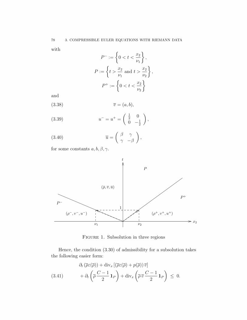
78 3. COMPRESSIBLE EULER EQUATIONS WITH RIEMANN DATA
with
P− :=
0 < t <
x2
ν1
,
P :=
t >
x2
ν1
and t >x2
ν2
,
P+ :=
0 < t <
x2
ν2
and
(3.38) v = (a, b),
(3.39) u− = u+ =
(12
0
0 −12
),
(3.40) u =
(β γ
γ −β
),
for some constants a, b, β, γ.
x2
P+
(ρ+, v+, u+)(ρ−, v−, u−)
P−
P
1
ν1 ν2
t
(ρ, v, u)
Figure 1. Subsolution in three regions
Hence, the condition (3.30) of admissibility for a subsolution takes
the following easier form:
∂t (ρε(ρ)) + divx [(ρε(ρ) + p(ρ)) v]
+ ∂t
(ρC − 1
21P
)+ divx
(ρ v
C − 1
21P
)≤ 0.(3.41)

3.6. NON–STANDARD SOLUTIONS WITH QUADRATIC PRESSURE 79
Inside each of the three regions P−, P and P+ the equations defining a
subsolution are trivially satisfied; hence they need to be imposed only
along fronts. If we plug in the choice of pressure law p(ρ) = ρ2, the
system (3.29) then reads as
ν2(ρ+ − ρ) = −bρ,(3.42a)
ν1(ρ− ρ−) = bρ,(3.42b)
ν2(ρ+ − ρa) = −γρ,(3.43a)
ν1(ρa+ ρ−) = γρ,(3.43b)
− ν2ρb = ρ+2 − ρ2 − Cρ
2+ ρβ,(3.43c)
ν1ρb = ρ2 − ρ−2+Cρ
2− ρβ.(3.43d)
Moreover, the relation between pressure and internal energy dictates
the analytical form of ε(ρ) in case p(ρ) = ρ2: we will simply have ε(ρ) =
ρ. Thus, the admissibility inequality (3.41) originates the following two
inequalities
ν2
(ρ2 − ρ+2
+ ρC − 1
2
)− b(
2ρ2 + ρC − 1
2
)≤ 0(3.44a)
ν1
(ρ−
2 − ρ2 − ρC − 1
2
)+ b
(2ρ2 + ρ
C − 1
2
)≤ 0.(3.44b)
Finally, the subsolution condition (3.28) in P translates into
(3.45)
(a2 − β ab− γab− γ b2 + β
)<
(C2
0
0 C2
).
3.6.1.2. Reduction of the admissibility condition.
Theorem 3.6.3. Let us suppose that
(3.46) ν1 < 0 < ν2.
Then, for the pressure function p(ρ) = ρ2, the admissibility conditions
(3.44a)-(3.44b) for a subsolution are implied by the following system of

80 3. COMPRESSIBLE EULER EQUATIONS WITH RIEMANN DATA
inequalities:
ρ ≤ ρ+ −√ρ+C − 1
2,(3.47a)
ρ ≥ ρ− +
√ρ−C − 1
2,(3.47b)
C > 1.(3.47c)
Indeed, the condition of admissibility (3.44a)-(3.44b) for the subso-
lution will be reduced to (3.47a)-(3.47c).
Proof . First, owing respectively to (3.42a) and (3.42b), we can
rewrite (3.44a) and (3.44b) as follows:
ν2
(ρ2 − ρ+2
+ ρC − 1
2
)+ ν2(ρ+ − ρ)
(2ρ+
C − 1
2
)≤ 0(3.48a)
ν1
(ρ−
2 − ρ2 − ρC − 1
2
)+ ν1(ρ− ρ−)
(2ρ+
C − 1
2
)≤ 0.(3.48b)
From the hypothesis (3.46) we can further reduce (3.48a)-(3.48b) to(ρ2 − ρ+2
+ ρC − 1
2
)+ (ρ+ − ρ)
(2ρ+
C − 1
2
)≤ 0(3.49a) (
ρ−2 − ρ2 − ρC − 1
2
)+ (ρ− ρ−)
(2ρ+
C − 1
2
)≥ 0.(3.49b)
Now, from (3.49a)- (3.49b), by simple algebra, we get
ρ2 − 2ρ+ρ+ ρ+2 − ρ+C − 1
2≥ 0(3.50a)
ρ2 − 2ρρ− + ρ−2 − ρ−C − 1
2≥ 0.(3.50b)
Clearly (3.50a) is satisfied if and only if
(3.51) ρ ≤ ρ+ −√ρ+C − 1
2∨ ρ ≥ ρ+ +
√ρ+C − 1
2,
while (3.50b) holds if and only if
(3.52) ρ ≤ ρ− −√ρ−C − 1
2∨ ρ ≥ ρ− +
√ρ−C − 1
2,
provided that C > 1, i.e. that (3.47c) holds. Observe from (3.42a)-
(3.42b) that
ν2(ρ+ − ρ) = −ν1(ρ− ρ−).
3.6. NON–STANDARD SOLUTIONS WITH QUADRATIC PRESSURE 81
Hence, in view of (3.46), either
(3.53) ρ− < ρ < ρ+
or
(3.54) ρ+ < ρ < ρ−
have to hold.
We assume to be in the first case, i.e. when (3.53) holds. Then
(3.51)-(3.52) respectively reduce to (3.47a)-(3.47b) as desired.
3.6.2. Proof of Theorem 3.6.1. This section is devoted to the
proof of Theorem 3.6.1: we will show that the set of all the conditions
required for an admissible subsolution to the compressible Euler system
has a solution. Since a lot of calculations are involved, we prefer to
split the proof in different parts, each of which corresponds to one of
the following subsections.
3.6.2.1. Change of variables. In this section we will rewrite the con-
ditions required to be an admissible subsolution for the compressible
Euler system in a new and more convenient set of variables.
First of all, by Theorem 3.6.3, the conditions of admissibility (3.44a)-
(3.44b) for the subsolution can be replaced with (3.47a)-(3.47b).
Resuming, we are looking for constants (ρ, ρ+, ρ−, ν1, ν2, a, b, β, γ, C)
satisfying (3.42a)-(3.42b), (3.43a)-(3.43d), (3.45), (3.47a)-(3.47c) and
such that
ν1 < 0 < ν2(3.55)
0 < ρ− < ρ < ρ+.(3.56)
Without loss of generality we can assume ρ = 1. Hence, (3.56) simpli-
fies to
(3.57) 0 < ρ− < 1 < ρ+,
while, (3.42a)-(3.43d) become
ν2(ρ+ − 1) = −b,(3.58a)
ν1(1− ρ−) = b,(3.58b)
82 3. COMPRESSIBLE EULER EQUATIONS WITH RIEMANN DATA
ν2(ρ+ − a) = −γ,(3.59a)
ν1(a+ ρ−) = γ,(3.59b)
− ν2b = ρ+2 − 1− C
2+ β,(3.59c)
ν1b = 1− ρ−2+C
2− β.(3.59d)
Finally, (3.47a)-(3.47b) take the form
ρ− +
√ρ−C − 1
2≤ 1(3.60a)
ρ+ −√ρ+C − 1
2≥ 1.(3.60b)
Owing to (3.57), the admissibility conditions (3.60a)-(3.60b) change
respectively into:
0 < ρ− ≤ 1
4
√(C − 1
2+ 4
)−√C − 1
2
2
(3.61a)
ρ+ ≥ 1
4
√(C − 1
2+ 4
)+
√C − 1
2
2
.(3.61b)
For the sake of simplicity, we introduce a new set of variables. We
define:
C := C/2, b := −b, γ := −γ, ν+ := ν2, ν− := −ν1
and
r+ := ρ+ν+, r− := ρ−ν−.
3.6. NON–STANDARD SOLUTIONS WITH QUADRATIC PRESSURE 83
This allows us to rewrite the ensemble of conditions (3.55), (3.57),
(3.58a)-(3.59d), (3.61a)-(3.61b) for an admissible subsolution as
ν−, ν+, b, r−, r+ > 0 and C > 1/2,(3.62)
r+ − ν+ = b,(3.63)
r− − ν− = −b,(3.64)
r+ − aν+ = γ,(3.65)
− r− − aν− = −γ,(3.66)
ν+b = ρ+2 − 1− C + β,(3.67)
ν−b = 1− ρ−2+ C − β,(3.68)
0 < ρ− ≤ 1
4
√(C +
7
2
)−√C − 1
2
2
,(3.69)
ρ+ ≥ 1
4
√(C +
7
2
)+
√C − 1
2
2
,(3.70)
while the subsolution condition (3.45) in P translates into
(3.71)
(C − a2 + β ab− γab− γ C − b2 − β
)> 0.
To summarize, we are looking for constants (r+, r−, ν+, ν−, a, b, β, γ, C)
satisfying (3.62)-(3.71).
3.6.2.2. Reduction of the equations. In this section, we work on the
system (3.62)-(3.71) so to simplify the conditions for an admissible
subsolution.
From (3.63) and (3.65) we obtain
ν+ =γ − b1− a
,(3.72)
r+ =γ − ab1− a
.(3.73)
Similarly (3.64) and (3.66) give
ν− =γ + b
1 + a,(3.74)
r− =γ − ab1 + a
.(3.75)
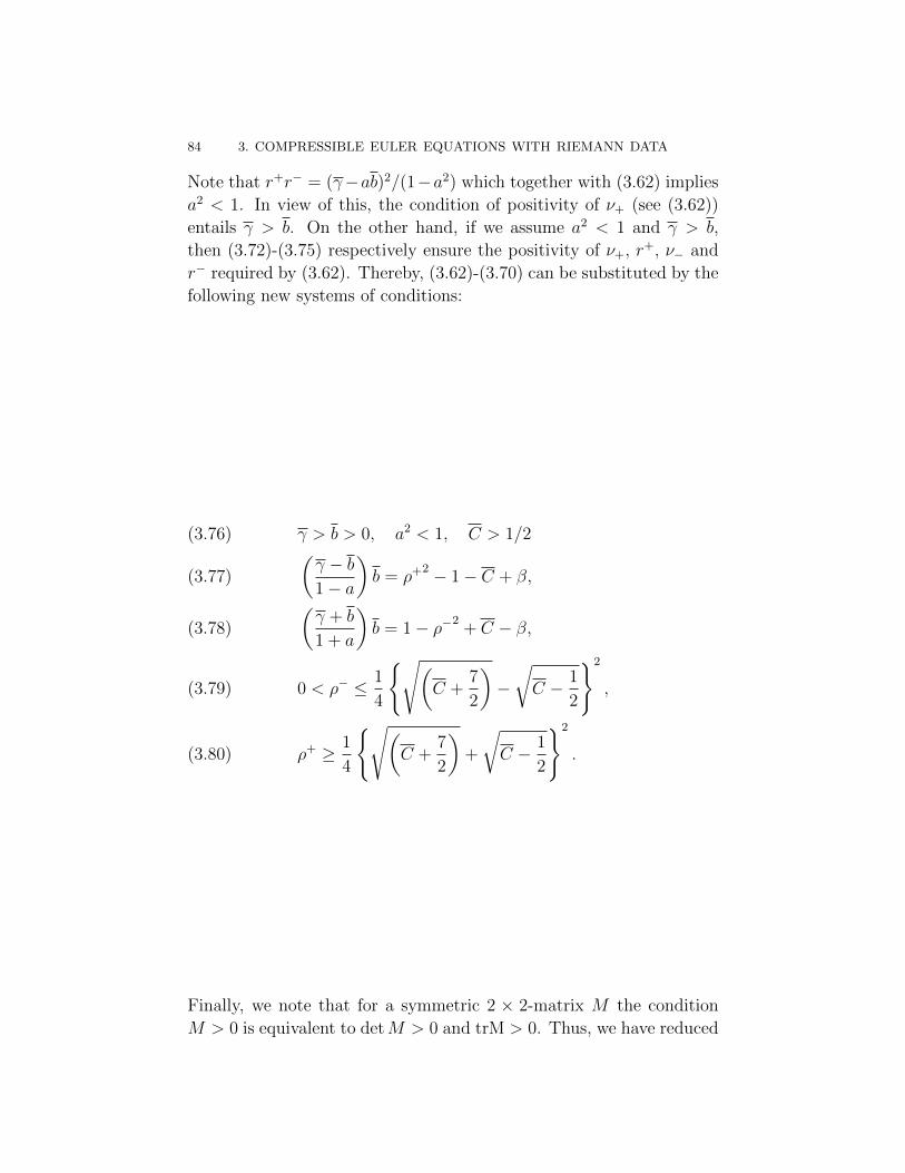
84 3. COMPRESSIBLE EULER EQUATIONS WITH RIEMANN DATA
Note that r+r− = (γ−ab)2/(1−a2) which together with (3.62) implies
a2 < 1. In view of this, the condition of positivity of ν+ (see (3.62))
entails γ > b. On the other hand, if we assume a2 < 1 and γ > b,
then (3.72)-(3.75) respectively ensure the positivity of ν+, r+, ν− and
r− required by (3.62). Thereby, (3.62)-(3.70) can be substituted by the
following new systems of conditions:
γ > b > 0, a2 < 1, C > 1/2(3.76) (γ − b1− a
)b = ρ+2 − 1− C + β,(3.77) (
γ + b
1 + a
)b = 1− ρ−2
+ C − β,(3.78)
0 < ρ− ≤ 1
4
√(C +
7
2
)−√C − 1
2
2
,(3.79)
ρ+ ≥ 1
4
√(C +
7
2
)+
√C − 1
2
2
.(3.80)
Finally, we note that for a symmetric 2 × 2-matrix M the condition
M > 0 is equivalent to detM > 0 and trM > 0. Thus, we have reduced

3.6. NON–STANDARD SOLUTIONS WITH QUADRATIC PRESSURE 85
the conditions for an admissible subsolution to:
γ > b > 0,(3.81)
a2 < 1,(3.82)
C >1
2,(3.83)
ρ+2=
(γ − b1− a
)b+ 1 + C − β,(3.84)
ρ−2
= −(γ + b
1 + a
)b+ 1 + C − β,(3.85)
0 < ρ− ≤ 1
4
√(C +
7
2
)−√C − 1
2
2
,(3.86)
ρ+ ≥ 1
4
√(C +
7
2
)+
√C − 1
2
2
,(3.87)
a2 + b2< 2C,(3.88)
(C − a2 + β)(C − b2 − β) > (γ − ab)2.(3.89)
3.6.2.3. Concluding argument. In view of the previous sections, in
order to prove Theorem 3.6.1 is enough to find constants (a, b, β, γ, C)

86 3. COMPRESSIBLE EULER EQUATIONS WITH RIEMANN DATA
satisfying:
γ > b > 0,
(3.90)
a2 < 1,
(3.91)
C >1
2,
(3.92)
0 <
√−(γ + b
1 + a
)b+ 1 + C − β ≤ 1
4
√(C +
7
2
)−√C − 1
2
2
,
(3.93)
√(γ − b1− a
)b+ 1 + C − β ≥ 1
4
√(C +
7
2
)+
√C − 1
2
2
,
(3.94)
a2 + b2< 2C,
(3.95)
(C − a2 + β)(C − b2 − β) > (γ − ab)2.
(3.96)

3.6. NON–STANDARD SOLUTIONS WITH QUADRATIC PRESSURE 87
To this aim, we further introduce a new variable λ := γ − ab, so
that (3.90)-(3.96) transform into the equivalent system:
λ > b(1− a) > 0,
(3.97)
a2 < 1,
(3.98)
C >1
2,
(3.99)
0 <
√− λb
1 + a− b2
+ 1 + C − β ≤ 1
4
√(C +
7
2
)−√C − 1
2
2
,
(3.100)
√λb
1− a− b2
+ 1 + C − β ≥ 1
4
√(C +
7
2
)+
√C − 1
2
2
,
(3.101)
a2 + b2< 2C,
(3.102)
(C − a2 + β)(C − b2 − β) > λ2.
(3.103)
Let us notice that, in view of (3.102) and (3.103), the following two
inequalities must hold
C − a2 + β > 0 and C − b2 − β > 0.

88 3. COMPRESSIBLE EULER EQUATIONS WITH RIEMANN DATA
Armed with the previous considerations, we now set C = 4/5b2
and
β = −2/5b2. Then, (3.97)-(3.103) transform into
λ > b(1− a) > 0,
(3.104)
a2 < 1,
(3.105)
b2>
5
8,
(3.106)
0 <
√− λb
1 + a+b
2
5+ 1 ≤ 1
4
√(4
5b
2+
7
2
)−√
4
5b
2 − 1
2
2
,
(3.107)
√λb
1− a+b
2
5+ 1 ≥ 1
4
√(4
5b
2+
7
2
)+
√4
5b
2 − 1
2
2
,
(3.108)
a2 <3
5b
2,
(3.109)
(2
5b
2 − a2
)b
2
5> λ2.
(3.110)
In conclusion, we are looking for (a, b, λ) such that (3.104)-(3.110) hold.
Let us make the choice b = 5, so that if there exist a and λ satisfying
the following set of conditions
λ > 5(1− a) > 0,(3.111)
a2 < 1,(3.112)
0 <
√6− 5λ
1 + a≤ 1
4
(43−
√1833
),(3.113) √
6 +5λ
1− a≥ 1
4
(43 +
√1833
),(3.114)
5(10− a2
)> λ2,(3.115)

3.7. NON–STANDARD SOLUTIONS WITH SPECIFIC PRESSURE 89
then we will obtain an admissible subsolution for the compressible Euler
equations. But it easy to check that conditions (3.111)-(3.115) admit
a solution (a, λ). Indeed, if we set a = 1 − ε for some ε > 0 to be
estimated, then (3.112) is immediately satisfied; on the other end the
remaining inequalities become:
λ > 5ε > 0,(3.116)
0 <
√6− 5λ
2− ε≤ 1
4
(43−
√1833
),(3.117) √
6 +5λ
ε≥ 1
4
(43 +
√1833
),(3.118)
5(9 + 2ε− ε2
)> λ2,(3.119)
Now, it is enough to plug in a small value for ε, for example ε = 1/100,
to check by hands that the region of λ’s satisfying (3.116)-(3.119) is
non empty, hence the proof of Theorem 3.6.1 is concluded.
3.7. Non–standard solutions with specific pressure
3.7.1. Construction of the subsolution. In this section, we
will prove the existence of an admissible subsolution for some specific
smooth pressure laws with p′ > 0, subsolution satisfying (3.33) too.
Theorem 3.7.1. There are a smooth pressure law p with p′ > 0 and
constants ρ± such that there exists an admissible subsolution (ρ, v, u) :
R2×]0,∞[→ (R+,R2,S2×20 ) to the compressible Euler equations with
(3.120) v(0) = v0, and ρ(0) = ρ0,
for ρ0 and v0 as in (3.22)-(3.23).
Remark 3.7.2. The admissible subsolution of Theorem 3.6.1 will
have the form
(ρ, v, u) =3∑i=1
(ρi, vi, ui)1Pi,
for some suitably chosen Pi, 1 ≤ i ≤ 3 as in the case of quadratic
pressure law.
What follows is devoted to the proof of Theorem 3.7.1.

90 3. COMPRESSIBLE EULER EQUATIONS WITH RIEMANN DATA
3.7.1.1. Subsolutions in three regions. We aim at constructing an
admissible subsolution to the compressible Euler equations of the fol-
lowing form (see Fig. 1):
(ρ, v, u) = (ρ−, v−, u−)1P−
+ (ρ, v, u)1P
+ (ρ+, v+, u+)1P+ ,(3.121)
with
P− :=
0 < t <
x2
ν1
,
P :=
t >
x2
ν1
and t >x2
ν2
,
P+ :=
0 < t <
x2
ν2
and
(3.122) v = (a, b),
(3.123) u− = u+ =
(12
0
0 −12
),
(3.124) u =
(β γ
γ −β
),
for some constants a, b, β, γ.
Hence, the condition (3.30) of admissibility for a subsolution takes
the following easier form:
∂t (ρε(ρ)) + divx [(ρε(ρ) + p(ρ)) v]
+ ∂t
(ρC − 1
21P
)+ divx
(ρv
C − 1
21P
)≤ 0.(3.125)
Inside each of the three regions P−, P and P+ the equations defining a
subsolution are trivially satisfied; hence they need to be imposed only
along fronts. The system (3.29) then reads as
ν2(ρ+ − ρ) = −bρ,(3.126a)
ν1(ρ− ρ−) = bρ,(3.126b)

3.7. NON–STANDARD SOLUTIONS WITH SPECIFIC PRESSURE 91
ν2(ρ+ − ρa) = −γρ,(3.127a)
ν1(ρa+ ρ−) = γρ,(3.127b)
− ν2ρb = p(ρ+)− p(ρ)− Cρ
2+ ρβ,(3.127c)
ν1ρb = p(ρ)− p(ρ−) +Cρ
2− ρβ.(3.127d)
The admissibility inequality (3.125) originates the following two in-
equalities
ν2
(ρε(ρ)− ρ+ε(ρ+) + ρ
C − 1
2
)− b(ρε(ρ) + p(ρ) + ρ
C − 1
2
)≤ 0
(3.128a)
ν1
(ρ−ε(ρ−)− ρε(ρ)− ρC − 1
2
)+ b
(ρε(ρ) + p(ρ) + ρ
C − 1
2
)≤ 0.
(3.128b)
Finally, the subsolution condition (3.28) in P translates into
(3.129)
(a2 − β ab− γab− γ b2 + β
)<
(C2
0
0 C2
).
3.7.1.2. Reduction of the admissibility condition.
Theorem 3.7.3. Let us suppose that
(3.130) ν1 < 0 < ν2.
Then, there exist pressure functions p ∈ C∞([0,+∞[) with p(0) =
p′(0) = 0 and p′ > 0 on ]0,+∞[ such that the admissibility conditions
(3.128a)-(3.128b) for a subsolution are implied by the following system
of inequalities: (p(ρ+)− p(ρ)
) (ρ+ − ρ
)≥ C − 1
2ρ+ρ(3.131a) (
p(ρ)− p(ρ−)) (ρ− ρ−
)≥ C − 1
2ρ−ρ.(3.131b)
The pressures p given by Theorem 3.7.3 will be chosen in Theorem
3.7.1 as the pressure law allowing room for the existence of an admissi-
ble subsolution. Indeed, thanks to the choice of such pressure laws the
condition of admissibility (3.128a)-(3.128b) for the subsolution will be
reduced to (3.131a)-(3.131b).
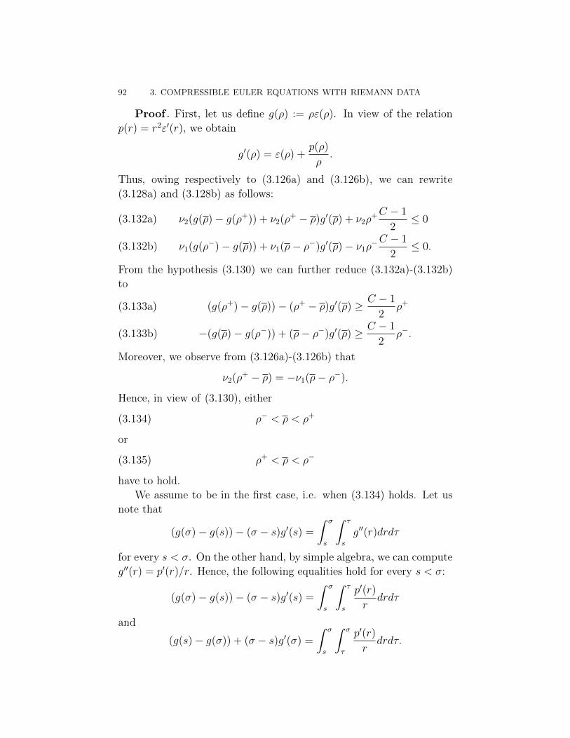
92 3. COMPRESSIBLE EULER EQUATIONS WITH RIEMANN DATA
Proof . First, let us define g(ρ) := ρε(ρ). In view of the relation
p(r) = r2ε′(r), we obtain
g′(ρ) = ε(ρ) +p(ρ)
ρ.
Thus, owing respectively to (3.126a) and (3.126b), we can rewrite
(3.128a) and (3.128b) as follows:
ν2(g(ρ)− g(ρ+)) + ν2(ρ+ − ρ)g′(ρ) + ν2ρ+C − 1
2≤ 0(3.132a)
ν1(g(ρ−)− g(ρ)) + ν1(ρ− ρ−)g′(ρ)− ν1ρ−C − 1
2≤ 0.(3.132b)
From the hypothesis (3.130) we can further reduce (3.132a)-(3.132b)
to
(g(ρ+)− g(ρ))− (ρ+ − ρ)g′(ρ) ≥ C − 1
2ρ+(3.133a)
−(g(ρ)− g(ρ−)) + (ρ− ρ−)g′(ρ) ≥ C − 1
2ρ−.(3.133b)
Moreover, we observe from (3.126a)-(3.126b) that
ν2(ρ+ − ρ) = −ν1(ρ− ρ−).
Hence, in view of (3.130), either
(3.134) ρ− < ρ < ρ+
or
(3.135) ρ+ < ρ < ρ−
have to hold.
We assume to be in the first case, i.e. when (3.134) holds. Let us
note that
(g(σ)− g(s))− (σ − s)g′(s) =
∫ σ
s
∫ τ
s
g′′(r)drdτ
for every s < σ. On the other hand, by simple algebra, we can compute
g′′(r) = p′(r)/r. Hence, the following equalities hold for every s < σ:
(g(σ)− g(s))− (σ − s)g′(s) =
∫ σ
s
∫ τ
s
p′(r)
rdrdτ
and
(g(s)− g(σ)) + (σ − s)g′(σ) =
∫ σ
s
∫ σ
τ
p′(r)
rdrdτ.

3.7. NON–STANDARD SOLUTIONS WITH SPECIFIC PRESSURE 93
As a consequence, and in view of (3.134), we can rewrite (3.133a) and
(3.133b) equivalently as∫ ρ+
ρ
∫ τ
ρ
p′(r)
rdrdτ ≥ C − 1
2ρ+,(3.136a) ∫ ρ
ρ−
∫ ρ
τ
p′(r)
rdrdτ ≥ C − 1
2ρ−.(3.136b)
Now, we introduce two new variables q+ and q− defined by
q+ := p(ρ+)− p(ρ),
q− := p(ρ)− p(ρ−).
Proving the Theorem is then equivalent to show the existence of a
pressure law p satisfying p(ρ+)− p(ρ) = q+, p(ρ)− p(ρ−) = q− and for
which the two inequalities (see (3.131a)-(3.131b))
q+(ρ+ − ρ
)≥ C − 1
2ρ+ρ(3.137a)
q−(ρ− ρ−
)≥ C − 1
2ρ−ρ.(3.137b)
imply (3.136a)-(3.136b) (which are equivalent to (3.128a)-(3.128b) as
just shown). In the following we will prove that such a choice of pressure
is possible. To this aim, we will introduce a measure theoretic setting.
First, we define the set of functions
L := f ∈ C∞([0,+∞[) such that f(0) = 0, f(r) > 0∀r ≥ 0 and∫ ρ
ρ−f = q−,
∫ ρ+
ρ
f = q+
and the two functional defined on L
L+(f) :=
∫ ρ+
ρ
∫ τ
ρ
f(r)
rdrdτ,
L−(f) :=
∫ ρ
ρ−
∫ ρ
τ
f(r)
rdrdτ.
Note that L is the set of derivatives of the possible pressure functions.
A necessary condition to find a pressure function p with the properties
above is that
l+ := supf∈L
L+(f) >C − 1
2ρ+

94 3. COMPRESSIBLE EULER EQUATIONS WITH RIEMANN DATA
and
l− := supf∈L
L−(f) >C − 1
2ρ−.
Let us generalize the space L as follows. We introduce
M+ :=
positive Radon measures µ on [ρ, ρ+] : µ([ρ, ρ+]) = q+,
M− :=
positive Radon measures µ on [ρ−, ρ] : µ([ρ−, ρ]) = q−.
Consistently, we extend the functionals L+ and L− defined on L to new
functionals L+ and L− respectively defined on M+ and on M−. We
define
L+(µ) :=
∫ ρ+
ρ
∫ τ
ρ
1
rdµ(r)dτ for µ ∈M+,
L−(µ) :=
∫ ρ
ρ−
∫ ρ
τ
1
rdµ(r)dτ for µ ∈M−.
Once introduced
m+ := maxµ∈M+
L+(µ)
and
m− := maxµ∈M−
L−(µ),
it is clear that
l+ ≤ m+ and l− ≤ m−.
Moreover, let us remark the existence of m± (i.e. that the maxima are
achieved) due to the compactness of M± with respect to the weak-∗topology. By a simple Fubini’s type argument, we write
L+(µ) =
∫ ρ+
ρ
ρ+ − rr
dµ(r).
Hence, defining the function h ∈ C([ρ, ρ+]) as h(r) := (ρ+−r)/r allows
us to express the action of the linear functional L+ as a duality pairing;
more precisely we have:
L+(µ) =< h, µ > for µ ∈M+.
Analougously, if we define g ∈ C([ρ−, ρ]) as g(r) := (r− ρ−)/r, we can
express L− as a duality pairing as well:
L−(µ) =< g, µ > for µ ∈M−.
By standard functional analysis, we know that m± must be achieved
at the extrem points ofM±. The extreme points ofM± are the single-
point measures, i.e. weighted Dirac masses. ForM+ the set of extrem

3.7. NON–STANDARD SOLUTIONS WITH SPECIFIC PRESSURE 95
points is then given by E+ := q+δσ for σ ∈ [ρ, ρ+] while for M− the
set of extrem points is then given by E− := q−δσ for σ ∈ [ρ−, ρ] In
order to find m±, it is enough to find the maximum value of L± on E±.
Clearly, we obtain
m+ = maxσ∈[ρ,ρ+]
q+ ρ+ − σ
σ
= q+ ρ+ − ρ
ρ
and
m− = maxσ∈[ρ−,ρ]
q−
σ − ρ−
σ
= q−
ρ− ρ−
ρ.
Furthermore, for every ε > 0 there exists a function f ∈ L such that
L+(f) > q+ ρ+ − ρρ− ε
and
L−(f) > q−ρ− ρ−
ρ− ε.
Such a function f is the derivative of the desired pressure function p.
Indeed, since f ∈ L, for p′(ρ) := f(ρ) we have: p(ρ+)− p(ρ) = q+ and
p(ρ) − p(ρ−) = q−. Finally, if (3.137a)-(3.137b) hold, then for every
ε > 0
L+(p′) ≥ C − 1
2ρ+ − ε
and
L−(p′) ≥ C − 1
2ρ− − ε,
whence (3.128a)-(3.128b).
3.7.2. Proof of Theorem 3.6.1. This section is devoted to the
proof of Theorem 3.7.1: we will show that the pressure law suggested
by Theorem 3.7.3 enable us to solve all the conditions required for an
admissible subsolution to the compressible Euler system. Since a lot
of calculations are involved, we will divide the proof in different parts
corresponding to different subsections.
3.7.2.1. Change of variables. In this section we will rewrite the con-
ditions required to be an admissible subsolution for the compressible
Euler system in a new and more convenient set of variables.
First of all, by Theorem 3.7.3, there is a choice of pressure law such
that the conditions of admissibility (3.128a)-(3.128b) for the subsolu-
tion can be replaced with (3.131a)-(3.131b).

96 3. COMPRESSIBLE EULER EQUATIONS WITH RIEMANN DATA
Resuming, we are looking for constants (ρ, ρ+, ρ−, ν1, ν2, a, b, β, γ, q+, q−, C)
satisfying (3.126a)-(3.126b), (3.127a)-(3.127d), (3.129), (3.131a)-(3.131b)
and such that
ν1 < 0 < ν2(3.138)
0 < ρ− < ρ < ρ+(3.139)
q+, q− > 0.(3.140)
Without loss of generality we can assume ρ = 1. Hence, (3.139) sim-
plifies to
(3.141) 0 < ρ− < 1 < ρ+,
while, (3.126a)-(3.127d) become
ν2(ρ+ − 1) = −b,(3.142a)
ν1(1− ρ−) = b,(3.142b)
ν2(ρ+ − a) = −γ,(3.143a)
ν1(a+ ρ−) = γ,(3.143b)
− ν2b = q+ − C
2+ β,(3.143c)
ν1b = q− +C
2− β.(3.143d)
Finally, (3.131a)-(3.131b) take the form
q+(ρ+ − 1
)≥ C − 1
2ρ+(3.144a)
q−(1− ρ−
)≥ C − 1
2ρ−.(3.144b)
From equations (3.142a)-(3.142b) we infer that
ρ+ − 1 = − b
ν2
,
(1− ρ−) =b
ν1
.

3.7. NON–STANDARD SOLUTIONS WITH SPECIFIC PRESSURE 97
Owing to previous equalities, the admissibility conditions (3.144a)-
(3.144b) change respectively into:
− b
ν2
q+ ≥ C − 1
2ρ+(3.145a)
b
ν1
q− ≥ C − 1
2ρ−.(3.145b)
For the sake of simplicity, we introduce a new set of variables. We
define:
C := C/2, b := −b, γ := −γ, ν+ := ν2, ν− := −ν1
and
r+ := ρ+ν+, r− := ρ−ν−.
This allows us to rewrite the ensemble of conditions (3.138), (5.22),
(3.141), (3.142a)-(3.143d), (3.145a)-(3.145b) for an admissible subsolu-
tion as
ν−, ν+, b, q−, q+, r−, r+ > 0,(3.146)
r+ − ν+ = b,(3.147)
r− − ν− = −b,(3.148)
r+ − aν+ = γ,(3.149)
− r− − aν− = −γ,(3.150)
ν+b = q+ − C + β,(3.151)
ν−b = q− + C − β,(3.152)
bq+ ≥(C − 1
2
)r+,(3.153)
bq− ≥(C − 1
2
)r−,(3.154)
while the subsolution condition (3.45) in P translates into
(3.155)
(C − a2 + β ab− γab− γ C − b2 − β
)> 0.
To summarize, we are looking for constants (r+, r−, ν+, ν−, a, b, β, γ, q+, q−, C)
satisfying (3.146)-(3.155).

98 3. COMPRESSIBLE EULER EQUATIONS WITH RIEMANN DATA
3.7.2.2. Reduction of the equations. In this section, we work on the
system (3.146)-(3.155) so to simplify the conditions for an admissible
subsolution.
From (3.147) and (3.149) we obtain
ν+ =γ − b1− a
,(3.156)
r+ =γ − ab1− a
.(3.157)
Similarly (3.148) and (3.150) give
ν− =γ + b
1 + a,(3.158)
r− =γ − ab1 + a
.(3.159)
Note that r+r− = (γ−ab)2/(1−a2) which together with (3.146) implies
a2 < 1. In view of this, the condition of positivity of ν+ (see (3.146))
entails γ > b. On the other hand, if we assume a2 < 1 and γ > b, then
(3.156)-(3.159) respectively ensure the positivity of ν+, r+, ν− and r−
required by (3.146). Thereby, (3.146)-(3.154) can be substituted by the
following new systems of conditions:
γ > b > 0, a2 < 1,(3.160)
q−, q+ > 0,(3.161) (γ − b1− a
)b = q+ − C + β,(3.162) (
γ + b
1 + a
)b = q− + C − β,(3.163)
bq+ ≥(C − 1
2
)(γ − ab1− a
),(3.164)
bq− ≥(C − 1
2
)(γ − ab1 + a
).(3.165)
Note that, if C > 1/2, then (3.160) and (3.164)-(3.165) guarantee the
positivity of q± (i.e. (3.161)). Hence, we can derive q± from (3.162)-
(3.163) and substitute them in (3.164)-(3.165). Finally, we note that
for a symmetric 2× 2-matrix M the condition M > 0 is equivalent to
detM > 0 and trM > 0. Thus, we have finally reduced the conditions

3.7. NON–STANDARD SOLUTIONS WITH SPECIFIC PRESSURE 99
for an admissible subsolution to:
γ > b > 0,(3.166)
a2 < 1,(3.167)
C >1
2,(3.168)
b
[b(γ − b)
1− a+ C − β
]≥(C − 1
2
)(γ − ab1− a
),(3.169)
b
[b(γ + b)
1 + a− C + β
]≥(C − 1
2
)(γ − ab1 + a
),(3.170)
a2 + b2< 2C,(3.171)
(C − a2 + β)(C − b2 − β)− (ab− γ)2 > 0.(3.172)
3.7.2.3. Concluding argument. In view of the previous sections, in
order to prove Theorem 3.7.1 is enough to find constants (a, b, β, γ, q+, q−, C)
satisfying (3.166)-(3.172). To this aim, we further introduce a new vari-
able λ := γ − ab, so that (3.166)-(3.172) transform into the equivalent
system:
λ > b(1− a) > 0,(3.173)
a2 < 1,(3.174)
C >1
2,(3.175)
b(1− a)(C − b2 − β
)≥(C − 1
2− b2
)λ,(3.176)
b(1 + a)(−C + b
2+ β
)≥(C − 1
2− b2
)λ,(3.177)
a2 + b2< 2C,(3.178)
(C − a2 + β)(C − b2 − β) > λ2.(3.179)
Now, from (3.178)-(3.179) follows that (C − b2− β) > 0; hence (3.177)
and (3.173) imply that (C − 1/2− b2) < 0, which automatically guar-
antees (3.176).

100 3. COMPRESSIBLE EULER EQUATIONS WITH RIEMANN DATA
Let us notice that if there exists a quadruple (a, b, C, β) satisfying
b > 0(3.180)
C >1
2(3.181)
a2 < 1,(3.182)
C − a2 + β > 0(3.183)
C − b2 − β > 0(3.184) (b
2+
1
2− C
)√C − a2 + β > b(1 + a)
√C − b2 − β(3.185) √(
C − a2 + β) (C − b2 − β
)> (1− a)b,(3.186)
then choosing λ :=
√(C − a2 + β
) (C − b2 − β
)− δ for δ > 0 small
enough, the quintuple (a, b, C, β, λ) satisfies (3.173)-(3.179).
Furthermore if (b, C, β) satisfy (3.180), (3.181), (3.184) and
C − 1 + β > 0(3.187) (b
2+
1
2− C
)√C − 1 + β > 2b
√C − b2 − β,(3.188)
then choosing a := 1− ε for ε > 0, they will satisfy (3.180)-(3.186).
Armed with the previous considerations, we now set C = 4/5b2
and
β = −2/5b2. Then (3.184) is automatically satisfied. The remaining
conditions (3.180), (3.181) and (3.187) are satisfied as soon as
(3.189) b >
√5
2.
Finally, with this choice of C and β, the inequality (3.188) is equivalent
to:
(3.190)
(b
2
5+
1
2
)√2b
2
5− 1 >
2b2
√5,
which holds surely in the limit for b → +∞. In conclusion, by choos-
ing b >√
5/3 big enough, C = 4/5b2, β = −2/5b
2, a = 1 − ε and
λ =
√(C − a2 + β
) (C − b2 − β
)− δ, for δ > 0 small enough, all the
conditions (3.173)-(3.179) are satisfied: we have proven the existence
3.7. NON–STANDARD SOLUTIONS WITH SPECIFIC PRESSURE 101
of an admissible subsolution for a particular choice of the pressure law
given by Theorem 3.7.3.


CHAPTER 4
Study of a classical Riemann problem for the
compressible Euler equations
This chapter is a complement to Chapter 3. Here we restrict our
attention to the 1-dimensional Riemann problem for the compressible
Euler equations with the same choice of initial data allowing for the
non–uniqueness theorems proven in Chapter 3 (see Theorem 0.2.2 or
Theorem 3.1.1) (such data indeed depend only on one space variable):
we show that such a problem admits unique self-similar solutions. In
particular we will investigate more deeply the case of quadratic pressure
law (as in Theorem 3.3.1) which is of easier treatise. The uniqueness of
self–similar solutions is proven by direct construction of the admissible
wave fun. Theorem 0.2.2 shows that as soon as the self–similarity
assumption runs out, uniqueness is lost.
4.1. Solution of the Riemann problem via wave curves
The property of first order conservation laws in one space-dimension
to be invariant under uniform stretching of the space-time coordinates
induces the existence of self-similar solutions, which stay constant along
straight-line rays emanating from the origin in space-time. This obser-
vation is at the core of the study of Riemann problems via wave fans.
Let us rewrite the isentropic Euler system (3.20) in canonical form,
i.e. in terms of the state variables (ρ,m) where m denotes the linear
momentum as was done in Chapter 2:
(4.1)
∂tρ+ divx(m) = 0
∂tm+ divx
(m⊗mρ
)+∇xp(ρ) = 0
ρ(·, 0) = ρ0
m(·, 0) = m0.
103
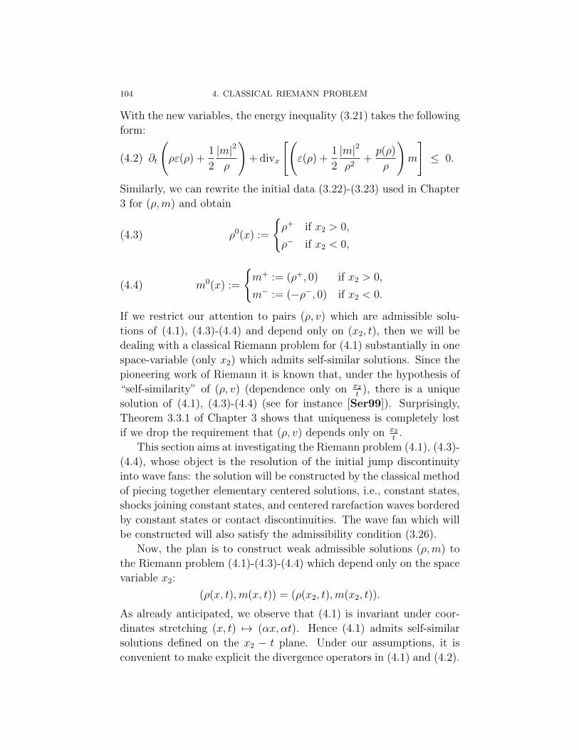
104 4. CLASSICAL RIEMANN PROBLEM
With the new variables, the energy inequality (3.21) takes the following
form:
(4.2) ∂t
(ρε(ρ) +
1
2
|m|2
ρ
)+ divx
[(ε(ρ) +
1
2
|m|2
ρ2+p(ρ)
ρ
)m
]≤ 0.
Similarly, we can rewrite the initial data (3.22)-(3.23) used in Chapter
3 for (ρ,m) and obtain
(4.3) ρ0(x) :=
ρ+ if x2 > 0,
ρ− if x2 < 0,
(4.4) m0(x) :=
m+ := (ρ+, 0) if x2 > 0,
m− := (−ρ−, 0) if x2 < 0.
If we restrict our attention to pairs (ρ, v) which are admissible solu-
tions of (4.1), (4.3)-(4.4) and depend only on (x2, t), then we will be
dealing with a classical Riemann problem for (4.1) substantially in one
space-variable (only x2) which admits self-similar solutions. Since the
pioneering work of Riemann it is known that, under the hypothesis of
“self-similarity” of (ρ, v) (dependence only on x2t
), there is a unique
solution of (4.1), (4.3)-(4.4) (see for instance [Ser99]). Surprisingly,
Theorem 3.3.1 of Chapter 3 shows that uniqueness is completely lost
if we drop the requirement that (ρ, v) depends only on x2t
.
This section aims at investigating the Riemann problem (4.1), (4.3)-
(4.4), whose object is the resolution of the initial jump discontinuity
into wave fans: the solution will be constructed by the classical method
of piecing together elementary centered solutions, i.e., constant states,
shocks joining constant states, and centered rarefaction waves bordered
by constant states or contact discontinuities. The wave fan which will
be constructed will also satisfy the admissibility condition (3.26).
Now, the plan is to construct weak admissible solutions (ρ,m) to
the Riemann problem (4.1)-(4.3)-(4.4) which depend only on the space
variable x2:
(ρ(x, t),m(x, t)) = (ρ(x2, t),m(x2, t)).
As already anticipated, we observe that (4.1) is invariant under coor-
dinates stretching (x, t) 7→ (αx, αt). Hence (4.1) admits self-similar
solutions defined on the x2 − t plane. Under our assumptions, it is
convenient to make explicit the divergence operators in (4.1) and (4.2).

4.1. SOLUTION OF THE RIEMANN PROBLEM VIA WAVE CURVES 105
Indeed, for ρ(x, t) = ρ(x2, t) and m(x, t) = (m1(x2, t),m2(x2, t)), we
can write the system (4.1) as
(4.5)
∂tρ+ ∂x2(m2) = 0
∂tm1 + ∂x2
(m1m2
ρ
)= 0
∂tm2 + ∂x2
(m2
2
ρ+ p(ρ)
)= 0
ρ(·, 0) = ρ0
m(·, 0) = m0,
while the energy inequality (4.2) becomes
(4.6) ∂t
(ρε(ρ) +
1
2
|m|2
ρ
)+ ∂x2
[(ε(ρ) +
1
2
|m|2
ρ2+p(ρ)
ρ
)m2
]≤ 0.
If (ρ,m) is a self-similar solution of (4.5), focused at the origin, its
restriction to t > 0 admits the representation
(4.7) (ρ,m)(x, t) = (R,M)(x2
t
), −∞ < x <∞, 0 < t <∞,
where (R,M) is a bounded measurable function on (−∞,∞), which
satisfies the ordinary differential equations
[M2(ξ)− ξR(ξ)]· +R(ξ) = 0[M1(ξ)M2(ξ)
R(ξ)− ξM1(ξ)
]·+M1(ξ) = 0[
M2(ξ)2
R(ξ)+ p(R(ξ))− ξM2(ξ)
]·+M2(ξ) = 0,
in the sense of distributions.
Before describing the structure of the solution to the Riemann prob-
lem, let us illustrate some general concepts concerning system (4.5). If
we define the state vector U := (ρ,m1,m2), we can recast the system
(4.5) in the general form
∂tU + ∂x2F (U) = 0,
where
F (U) :=
m2m1m2
ρm2
2
ρ+ p(ρ)
.

106 4. CLASSICAL RIEMANN PROBLEM
By definition (cf. [Daf00]) the system (4.5) is hyperbolic since the
Jacobian matrix DF (U)
DF (U) =
0 0 1−m1m2
ρ2m2
ρm1
ρ−m2
2
ρ2+ p′(ρ) 0 2m2
ρ
has real eigenvalues
(4.8) λ1 =m2
ρ−√p′(ρ), λ2 =
m2
ρ, λ3 =
m2
ρ+√p′(ρ)
and 3 linearly independent eigenvectors
(4.9)
R1 =
1m1
ρm2
ρ−√p′(ρ)
, R2 =
0
1
0
, R3 =
1m1
ρm2
ρ+√p′(ρ)
.
The eigenvalue λi of DF , i = 1, 2, 3, is called the i-characteristic speed
of the system (4.5). On the part of the state space of our interest, with
ρ > 0, the system (4.5) is indeed strictly hyperbolic. Finally, one can
easily verify that the functions
(4.10)
w1 =m2
ρ+
∫ ρ
0
√p′(τ)
τdτ, w2 =
m1
ρ, w3 =
m2
ρ−∫ ρ
0
√p′(τ)
τdτ
are, respectively, 1− and 2−, 1− and 3−, 2− and 3− Riemann in-
variants of the system (4.5) (for the relevant definitions see [Daf00]).
In other words there exist two 1−Riemann invariants w1 and w2, two
2−Riemann invariants w1 and w3 and two 3−Riemann invariants w2
and w3.
We close this section with a key observation: note that the state
variable m1 appears only in the second equation of the system (4.5).
We can thus “decouple” the study of the first and third equations in
(4.5) from the study of the second one: this is possible by performing a
sort of “projection” operation on the ρ−m2-plane. More precisely, we
will first construct solutions (ρ,m2) and then analyze the behaviour of
m1 determined by the second equation in (4.5).

4.2. THE HUGONIOT LOCUS 107
4.2. The Hugoniot locus
We focus our attention on the reduced system
(4.11)
∂tρ+ ∂x2(m2) = 0
∂tm2 + ∂x2
(m2
2
ρ+ p(ρ)
)= 0
ρ(·, 0) = ρ0
m2(·, 0) = (m0)2,
obtained by discarding the second equation in (4.5). Note that, if we
define the state variable U = (ρ,m2) and we formally recast the system
(4.11) in the form ∂tU + ∂x2G(U) = 0 for U = P1,3U , then we have
G(U) = P1,3F (U) and DG(U) = P1,3DF (U)P T1,3 (D = DU), where P1,3
is the following matrix:
P1,3 =
(1 0 0
0 0 1
).
Hence, the characteristic speeds of the system (4.11) are λ1 and λ3
with associated eigenvectors P1,3 ·R1 and P1,3 ·R3 (see (4.8)-(4.9)). The
Hugoniot locus of the reduced system (4.11) is the set of points U2 =
(ρ,m2) that may be joined to a fixed point U1 = (ρ,m2) by a shock. In
view of the previous remark, we can observe that Hugoniot loci of the
reduced system (4.11) correspond to projections on the ρ−m2- plane
of Hugoniot loci of the full system (4.5). In our case, we can describe
the Hugoniot locus for (4.11) explicitly by computing the Rankine-
Hugoniot jump conditions:
G(U2)−G(U1) = σ(U2 − U1),
which can be written, for U1, U2 such that U1 = P1,3U1 and U2 = P1,3U2,
as
P1,3[F (U2)− F (U1)] = P1,3σ(U2 − U1).
Note, that the set of equations [F (U2)−F (U1)] = σ(U2−U1) describes
indeed the Hugoniot locus of the full system (4.5).
Now, we would like to investigate the Hugoniot locus of the state
(ρ−,m−). We start by studying its projection on the ρ − m2-plane,
i.e. by computing the Hugoniot locus of system (4.11). The state
(ρ−, (m−)2) = (ρ−, 0) on the left is joined to the state (ρ,m2) on the

108 4. CLASSICAL RIEMANN PROBLEM
right, by a shock of speed σ if the following equations hold:
(4.12)
−σ(ρ− ρ−) +m2 = 0
−σm2 + m22
ρ+ p(ρ)− p(ρ−) = 0.
We can now restrict ourselves to the case of a polytropic pressure law,
with adiabatic exponent γ = 2 for which the non-uniqueness result
3.3.1 stated in Chapter 3 holds. Thus, from now on we will assume
that
p(r) = kr2
for some positive constant k. As a consequence, the Rankine-Hugoniot
conditions (4.12) take the form
(4.13)
−σ(ρ− ρ−) +m2 = 0
−σm2 + m22
ρ+ kρ2 − k(ρ−)
2= 0.
From (4.13) we infer that
(4.14) σ = ±
√kρ(ρ+ ρ−)
ρ−.
Recalling the characteristic speeds λ1 and λ3 for the system (4.11), it is
natural to call shocks propagating to the left (σ1 = −√kρ(ρ+ ρ−)/ρ− <
0) 1-shocks and shocks propagating to the right (σ3 =√kρ(ρ+ ρ−)/ρ− >
0) 3-shocks. Combining (4.13) with (4.14) we deduce that the Hugoniot
locus of the point (ρ−, 0) in state space consists of two curves:
(4.15) m2 = ±
√kρ (ρ+ ρ−)
ρ−(ρ− ρ−
),
defined on the whole range of ρ > 0. Moreover a 1-shock joining
(ρ−, 0) on the left to (ρ,m2) on the right is admissible, i.e. it satisfies
the entropy condition (4.2) if and only if ρ− < ρ. While a 3-shock
joining the state (ρ,m2) on the left with the state (ρ+, 0) on the right
is admissible if and only if ρ > ρ+.
4.3. Rarefaction waves
In order to characterize rarefaction waves of the reduced system
(4.11), we can refer to Theorem 7.6.6 from [Daf00]: every i-Riemann
invariant is constant along any i-rarefaction wave curve of the system
(4.11) and conversely the i- rarefaction wave curve, through a state
4.5. SOLUTION OF THE RIEMANN PROBLEM 109
(ρ,m2) of genuine nonlinearity of the i-characteristic family, is deter-
mined implicitly by the system of equations wi(ρ,m2) = wi(ρ,m2) for
every i−Riemann invariant wi. As an application of this Theorem, we
obtain that the 1- and 3-rarefaction wave curves of the system (4.11)
through the point (ρ−, 0) are determined respectively in terms of the
Riemann invariants w1 and w3 by the equations
(4.16) m2 = 2ρ√
2k(√ρ− −√ρ), m2 = 2ρ
√2k(√ρ−
√ρ−).
Similarly, we can obtain the rarefaction waves through the point (ρ+, 0).
As already discussed for the Hugoniot locus, the rarefaction waves here
obtained for the reduced system (4.11) correspond to projections on the
ρ −m2-plane of rarefaction waves of (4.5). In order to determine the
first component of the linear momentum along the rarefaction waves
we will make use of the second Riemann invariant w2 for the complete
system (4.5).
4.4. Contact discontinuity
It is easy to verify that the 2-characteristic family of the system
(4.5) is linearly degenerate, i.e. Dλ2 · R2 = 0. As a consequence, no
centered 2-rarefaction waves for the system (4.5) exist and hence any 2-
wave is necessarily a 2-contact discontinuity. A 2-contact discontinuity
is a shock traveling at characteristic speed λ2 (see (4.8)) and such that
the only variable which experiences a jump is the first component of
the linear momentum. The entropy condition holds trivially across the
contact discontinuity, for the rate of production of entropy is indeed
zero.
4.5. Solution of the Riemann problem
According to Theorem 9.3.1 in [Daf00] any self-similar solution of
the Riemann problem (4.5), (4.3)-(4.4), with shocks satisfying the en-
tropy inequality, comprises 4 constant states U0 = (ρ0,m0) = (ρ−,m−),
U1, U2, U3 = (ρ+,m+). For i = 1, 2, 3, Ui−1 is joined to Ui by an i-wave.
In the following we will construct such a self-similar solution by
piecing together shocks, rarefaction waves and contact discontinuities
obtained in the previous sections. As in the literature, we will call for-
ward (or backward) i-wave fan curve through (ρ,m) the Lipschitz curve
Φi(·, (ρ,m)) (or Ψi(·, (ρ,m))) describing the locus of states that may
110 4. CLASSICAL RIEMANN PROBLEM
be joined on the right (or left) of the fixed state (ρ,m) by an admis-
sible i-wave fan. Clearly, we could obtain a solution of our Riemann
problem starting from (ρ−,m−) and computing successively the states
(ρi,mi) = Φi(·, (ρi,mi)) until we reach (ρ+,m+). In our circumstances,
a “mixed” strategy proves to be advantageous. We will first consider
the system (4.11) of two conservation laws in the two variables (ρ,m2),
then we will draw for it the forward 1-wave curve through the left state
(ρ−, 0) and the backward 3-wave curve through the right state (ρ+, 0)
and finally we will determine the intermediate state as the intersec-
tion of these two curves. In order to complete the picture, we will
introduce a 2-contact discontinuity accounting for the jump in the first
component of the linear momentum.
Recalling the form of the Hugoniot locus (4.15) and rarefaction wave
curves (4.16) for system (4.11), we deduce that we can parametrize the
wave curves employing ρ as the parameter. Thus, the forward 1-wave
curve m2 = Φ1(ρ; (ρ−, 0)) through the point (ρ−, 0) consists of a 1-
rarefaction wave for ρ− ≥ ρ and an admissible 1-shock for ρ− < ρ:
(4.17) m2 = Φ1(ρ; (ρ−, 0)) =
2ρ√
2k(√ρ− −√ρ) if ρ− ≥ ρ
−√
kρ(ρ+ρ−)ρ−
(ρ− ρ−) if ρ− < ρ.
On the other hand, the backward 3-wave curve through the point
(ρ+, 0) is composed of a 3-rarefaction wave for ρ+ ≥ ρ and an ad-
missible 3-shock for ρ+ < ρ:
(4.18) m2 = Ψ3(ρ; (ρ+, 0)) =
−2ρ√
2k(√ρ+ −√ρ) if ρ+ ≥ ρ√
kρ(ρ+ρ+)ρ+
(ρ− ρ+) if ρ+ < ρ.
The intermediate constant state (ρM ,mM) is determined on the ρ−m2
plane as the intersection of the forward 1-wave curve Φ1(ρ; (ρ−, 0))
with the backward 3-wave curve Ψ3(ρ; (ρ+, 0)) (see Fig. 1), namely by
solving the equation
mM = Φ1(ρM ; (ρ−, 0)) = Ψ3(ρM ; (ρ+, 0)).
Note that such intersection is unique (if ρ > 0), since Φ1 is a strictly
decreasing function in ρ for ρ > 4/9ρ− with Φ1 > 0 for 0 < ρ < ρ−,
while Ψ3 is a strictly increasing function of ρ for ρ > 4/9ρ+, always
strictly convex and negative for every 0 < ρ < ρ+.

4.5. SOLUTION OF THE RIEMANN PROBLEM 111
(ρ−, 0)ρ
(ρ+, 0)
1-rarefaction wave
Φ1(ρ; (ρ−, 0))
m2
Ψ3(ρ; (ρ+, 0))
3-shock
(ρM ,mM )
1-shock
3-rarefaction wave
Figure 1. ρ−m2 plane
So far, we have discussed the resolution of the reduced system
(4.11), thus obtaining a complete description of the behavior of the den-
sity and of the second component of the linear momentum. Now, also
the second equation of (4.5) governing the first component of the linear
momentum has to come into play. By imposing the Rankine-Hugoniot
condition corresponding to the second equation of (4.5) across the 1-
shock traveling at speed σ1, we can compute the uniquely determined
value of the first component of the linear momentum of the second
constant state U1 and we obtain
U1 = (ρM , (−ρM ,mM)).
The second state U1 is then joined to the third state U2 by a 2-contact
discontinuity traveling at speed σ2 = mM/ρM . Note that σ2 ≥ σ1. The
entropy condition for the 2-contact discontinuity is always satisfied
since across it the rate of production of entropy is zero. Moreover, the
only variable which jumps across the 2-contact discontinuity is the first
component of the linear momentum. Hence, U2 has the form
U2 = (ρM , (n,mM)),
with n to be determined later. Finally, the third state U2 will be joined
to U3 = (ρ+,m+) by a 3- rarefaction wave. As previously explained,
along a 3-rarefaction wave all the 3−Riemann invariants have to stay
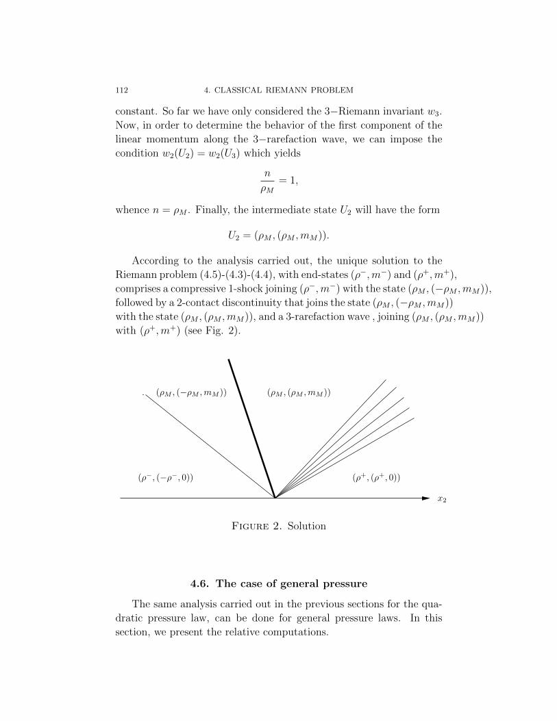
112 4. CLASSICAL RIEMANN PROBLEM
constant. So far we have only considered the 3−Riemann invariant w3.
Now, in order to determine the behavior of the first component of the
linear momentum along the 3−rarefaction wave, we can impose the
condition w2(U2) = w2(U3) which yields
n
ρM= 1,
whence n = ρM . Finally, the intermediate state U2 will have the form
U2 = (ρM , (ρM ,mM)).
According to the analysis carried out, the unique solution to the
Riemann problem (4.5)-(4.3)-(4.4), with end-states (ρ−,m−) and (ρ+,m+),
comprises a compressive 1-shock joining (ρ−,m−) with the state (ρM , (−ρM ,mM)),
followed by a 2-contact discontinuity that joins the state (ρM , (−ρM ,mM))
with the state (ρM , (ρM ,mM)), and a 3-rarefaction wave , joining (ρM , (ρM ,mM))
with (ρ+,m+) (see Fig. 2).
x2
(ρM , (−ρM ,mM ))
(ρ+, (ρ+, 0))
(ρM , (ρM ,mM ))
(ρ−, (−ρ−, 0))
Figure 2. Solution
4.6. The case of general pressure
The same analysis carried out in the previous sections for the qua-
dratic pressure law, can be done for general pressure laws. In this
section, we present the relative computations.
4.6. THE CASE OF GENERAL PRESSURE 113
4.6.1. The Hugoniot locus. As before, we deal with the reduced
system (4.11). From (4.13) we infer that for general pressure p:
(4.19) σ = ±
√ρ(p(ρ)− p(ρ−))
ρ−(ρ− ρ−).
Recalling the characteristic speeds λ1 and λ3 for the system (4.11), it is
natural to call shocks propagating to the left(σ1 = −
√ρ(p(ρ)−p(ρ−))ρ−(ρ−ρ−)
< 0)
1-shocks and shocks propagating to the right(σ3 =
√ρ(p(ρ)−p(ρ−))ρ−(ρ−ρ−)
> 0)
3-shocks. Combining (4.13) with (4.19) we deduce that the Hugoniot
locus of the point (ρ−, 0) in state space consists of two curves:
(4.20) m2 = ±
√ρ(p(ρ)− p(ρ−))
ρ−(ρ− ρ−)
(ρ− ρ−
),
defined on the whole range of ρ > 0. Moreover a 1-shock joining
(ρ−, 0) on the left to (ρ,m2) on the right is admissible, i.e. it satisfies
the entropy condition (4.2) if and only if ρ− < ρ. While a 3-shock
joining the state (ρ,m2) on the left with the state (ρ+, 0) on the right
is admissible if and only if ρ > ρ+.
4.6.2. Rarefaction waves. By use of Theorem 7.6.6 from [Daf00]
the i- rarefaction wave curve, through a state (ρ,m2) of genuine non-
linearity of the i-characteristic family, is determined implicitly by the
system of equations wi(ρ,m2) = wi(ρ,m2). As an application of this
Theorem, we obtain that the 1- and 3-rarefaction wave curves of the
system (4.11) through the point (ρ−, 0) are respectively determined in
terms of the Riemann invariants w1 and w3 by the equations
(4.21) m2 = ρ
∫ ρ−
ρ
√p′(τ)
τdτ, m2 = ρ
∫ ρ
ρ−
√p′(τ)
τdτ.
The rarefaction waves through the point (ρ+, 0) can be obtained in a
similar way.
4.6.3. Contact discontinuity. As already pointed out, the 2-
characteristic family of the system (4.5) is linearly degenerate, i.e. Dλ2·R2 = 0. Any 2-wave is a 2-contact discontinuity, i.e. a shock traveling
at characteristic speed λ2. Along the 2-contact discontinuity a jump
in the first component of the linear momentum occurs. The entropy

114 4. CLASSICAL RIEMANN PROBLEM
condition holds trivially across the contact discontinuity, for the rate
of production of entropy is indeed zero.
4.6.4. Solution of the Riemann problem. As done in Section
4.5, we will apply Theorem 9.3.1 in [Daf00]. The definitions as well as
the strategies introduced in Section 4.5 are valid also herein.
Recalling the form of the Hugoniot locus (4.20) and rarefaction wave
curves (4.21) for system (4.11) with general pressure laws, we deduce
that we can parametrize the wave curves employing ρ as the parameter.
Thus, the forward 1-wave curve m2 = Φ1(ρ; (ρ−, 0)) through the point
(ρ−, 0) consists of a 1-rarefaction wave for ρ− ≥ ρ and an admissible
1-shock for ρ− < ρ:
(4.22) m2 = Φ1(ρ; (ρ−, 0)) =
ρ∫ ρ−ρ
√p′(τ)
τdτ if ρ− ≥ ρ
−√
ρ(p(ρ)−p(ρ−))ρ−(ρ−ρ−)
(ρ− ρ−) if ρ− < ρ.
On the other hand, the backward 3-wave curve through the point
(ρ+, 0) is composed of a 3-rarefaction wave for ρ+ ≥ ρ and an ad-
missible 3-shock for ρ+ < ρ:
(4.23) m2 = Ψ3(ρ; (ρ+, 0)) =
−ρ∫ ρ+ρ
√p′(τ)
τdτ if ρ+ ≥ ρ√
ρ(p(ρ)−p(ρ+))ρ+(ρ−ρ+)
(ρ− ρ+) if ρ+ < ρ.
The intermediate constant state (ρM ,mM) is determined on the ρ−m2
plane as the intersection of the forward 1-wave curve Φ1(ρ; (ρ−, 0)) with
the backward 3-wave curve Ψ3(ρ; (ρ+, 0)), namely by the equation
mM = Φ1(ρM ; (ρ−, 0)) = Ψ3(ρM ; (ρ+, 0)).
We argue that such intersection is unique for the choice of pressure
functions as in Theorem 3.7.3 of Chapter 3. Indeed mM is uniquely
determined, since Φ1 is a strictly decreasing function in ρ with Φ1 > 0
for 0 < ρ < ρ−, while Ψ3 is negative for every 0 < ρ < ρ+ with Ψ3
convex for ρ < ρ and concave for ρ > ρ, where ρ is a density-value in
a small neighborhood of 1 (recall from Section 3.7.2 of Chapter 3 that
in the construction of the subsolution we chose ρ = 1).
By imposing the Rankine-Hugoniot condition corresponding to the
second equation of (4.5) across the 1-shock traveling at speed σ1, we
can compute the uniquely determined value of the first component of
4.6. THE CASE OF GENERAL PRESSURE 115
the linear momentum of the second constant state U1 and we obtain
U1 = (ρM , (−ρM ,mM)).
The second state U1 is then joined to the third state U2 by a 2-contact
discontinuity traveling at speed σ2 = mM/ρM . Note that σ2 ≥ σ1. The
entropy condition for the 2-contact discontinuity is always satisfied
since across it the rate of production of entropy is zero. Moreover, the
only variable which jumps across the 2-contact discontinuity is the first
component of the linear momentum. Hence, U2 has the form
U2 = (ρM , (n,mM)),
with n to be determined later. Finally, the third state U2 will be joined
to U3 = (ρ−,m−) by a 3- rarefaction wave along which the Riemann
invariant w2 has to stay constant: w2(U2) = w2(U3), i.e.n
ρM= 1.
This implies that n = ρM , whence
U2 = (ρM , (ρ+,mM)).
The unique solution to the Riemann problem (4.5)-(4.3)-(4.4) for
pressure laws as in Theorem ??, with end-states (ρ−,m−) and (ρ+,m+),
comprises a compressive 1-shock joining (ρ−,m−) with the state (ρM , (−ρM ,mM)),
followed by a 2-contact discontinuity that joins the state (ρM , (−ρM ,mM))
with the state (ρM , (ρ+,mM)), and a 3-rarefaction wave , joining (ρM , (ρ
+,mM))
with (ρ+,m+) (see Fig. 2), as in the case of quadratic pressure.


CHAPTER 5
Existence of weak solutions
5.1. Introduction
The result presented in this Chapter stems from an idea recently ex-
plored by Emil Wiedemann for the incompressible Euler equations. In
[Wie11] Wiedemann shows existence of weak solutions to the Cauchy
problem for the incompressible Euler equations with general initial data
(see Chapter 1). His proof combines some Fourier analysis with a clever
application of the methods developed by De Lellis and Szekelyhidi in
[DLS09]-[DLS10] for the construction of non-standard solutions to the
incompressible Euler equations. The conclusions achieved in [Chi11]
and presented in Chapter 2 for the compressible Euler system gave hope
that such an existence result could hold also for isentropic compressible
gas dynamics in several space dimensions.
The existence of entropy solutions for the Cauchy problem asso-
ciated with the isentropic compressible Euler equations in one space
dimension was established, in the case of polytropic perfect gases first
by DiPerna [DP85], Ding, Chen & Luo [DCL85], and Chen [Che86]
based on compensated compactness arguments, and then, motivated
by a kinetic formulation of hyperbolic conservation laws, by Lions,
Perthame & Tadmor [LPT94], and Lions, Perthame & Souganidis
[LPS96]. General pressure laws were covered first by Chen & LeFloch
[CL00]. Unlike in the one-dimensional case, the existence problem
for weak solutions of multi-dimensional isentropic gas dynamics has
remained open so far.
The outcome of [Wie11] hints that the powerful approach by De
Lellis and Szekelyhidi is not only a “generator” of nonuniqueness, but
can actually be exploited to construct weak solutions starting out from
any initial data (see also [DLS11])! Here, we will follow such a hint and
building upon results from [Chi11]-[DLS10]-[Wie11] we will show ex-
istence of weak solutions to the compressible Euler equations for any
117

118 5. EXISTENCE OF WEAK SOLUTIONS
Lipschitz continuous initial density and any bounded initial momen-
tum.
Theorem 5.1.1. Let ρ0 ∈ C1p(Q;R+) and m0 ∈ H(Q). Then there
exists a weak solution (ρ,m) (in fact, infinitely many) of the Cauchy
problem for the compressible Euler equations with intial data (ρ0,m0).
Of course, the optimal result would be existence of weak solutions
starting out from any bounded initial data: Theorem 5.1.1 is a just a
first step towards this.
5.2. The problem
In this section, we formulate the isentropic compressible Euler equa-
tions of gas dynamics in n space dimensions, n ≥ 2 (cf. Section 3.3 of
[Daf00]) and in canonical form (as in Chapter 2). The system, which
consists of n+ 1 equations, takes the form:
(5.1)
∂tρ+ divxm = 0
∂tm+ divx
(m⊗mρ
)+∇x[p(ρ)] = 0
ρ(·, 0) = ρ0
m(·, 0) = m0
,
where ρ is the density and m the linear momentum field. The pressure
p is a function of ρ determined from the constitutive thermodynamic
relations of the gas in question. The system is hyperbolic if
p′(ρ) > 0.
We will consider, from now on, the case of general pressure laws given
by a function p on [0,∞[, that we always assume to be continuously
differentiable on [0,∞[ and strictly increasing on [0,∞[.
Here, as in Chapter 2, we work with space periodic boundary condi-
tions. For space periodic flows we assume that the fluid fills the entire
space Rn but with the condition that m, ρ are periodic functions of the
space variable.
Let Q = [0, 1]n, n ≥ 2 be the unit cube in Rn. We denote by
Hmp (Q), m ∈ N, the space of functions which are in Hm
loc(Rn) and
which are periodic with period Q:
m(x+ l) = m(x) for a.e. x ∈ Rn and every l ∈ Zn.
For m = 0, H0p (Q) coincides simply with L2(Q). Analogously, for every
functional space X we define Xp(Q) to be the space of functions which
5.2. THE PROBLEM 119
are locally (over Rn) in X and are periodic of period Q. The functions
in Hmp (Q) are easily characterized by their Fourier series expansion
(5.2)
Hmp (Q) =
m ∈ L2
p(Q) :∑k∈Zn
|k|2m |m(k)|2 <∞ and m(0) = 0
,
where m : Zn → Cn denotes the Fourier transform of m. We will use
the notation H(Q) for H0p (Q) and Hw(Q) for the space H(Q) endowed
with the weak L2 topology.
Let T be a fixed positive time. By a weak solution of (5.1) on
Rn × [0, T [ we mean a pair (ρ,m) ∈ L∞([0, T [;L∞p (Q)) satisfying
(5.3)
|m(x, t)| ≤ Rρ(x, t) for a.e. (x, t) ∈ Rn × [0, T [ and some R > 0,
and such that the following identities hold for every test functions ψ ∈C∞c ([0, T [;C∞p (Q)), φ ∈ C∞c ([0, T [;C∞p (Q)):
(5.4)
∫ T
0
∫Q
[ρ∂tψ +m · ∇xψ] dxdt+
∫Q
ρ0(x)ψ(x, 0)dx = 0
∫ T
0
∫Q
[m · ∂tφ+
⟨m⊗mρ
,∇xφ
⟩+ p(ρ) divx φ
]dxdt
+
∫Q
m0(x) · φ(x, 0)dx = 0.(5.5)
In the following, we will be dealing also with the semi-stationary
Cauchy problem associated with the isentropic Euler equations (simply
set to 0 the time derivative of the density in (5.1) and drop the initial
condition for ρ):
(5.6)
divxm = 0
∂tm+ divx
(m⊗mρ
)+∇x[p(ρ)] = 0
m(·, 0) = m0.
A pair (ρ,m) ∈ L∞p (Q)×L∞([0, T [;L∞p (Q)) is a weak solution on Rn×[0, T [ of (2.8) if m(·, t) is weakly-divergence free for almost every 0 <
t < T and satisfies the following bound
(5.7)
|m(x, t)| ≤ Rρ(x) for a.e. (x, t) ∈ Rn × [0, T [ and some R > 0,
and if the identity (3.25) holds for every φ ∈ C∞c ([0, T [;C∞p (Q)).
120 5. EXISTENCE OF WEAK SOLUTIONS
5.3. Existence of weak solutions
5.3.1. Background results. Before stating and proving the main
theorem, we recall a Proposition from [Chi11] which represents the
building block of our argument. For the sake of completeness of the
chapter, we report Proposition 4.1 from [Chi11] which is Proposition
2.4.1 in Chapter 2. A similar criterion was proposed by De Lellis and
Szekelyhidi for the incompressible Euler equations (see [DLS10]) and
used by Wiedemann in his proof of existence of weak solutions for
incompressible Euler in [Wie11].
Proposition 5.3.1. Let ρ ∈ C1p(Q;R+) be any given density func-
tion and let T be any positive time.
Assume there exist (m,U, q) continuous space-periodic solutions of
divxm = 0
∂tm+ divx U +∇xq = 0.(5.8)
on Rn×]0, T [ with
(5.9) m ∈ C([0, T ];Hw(Q)),
and a function χ ∈ C∞([0, T ];R+) such that
λmax
(m(x, t)⊗m(x, t)
ρ(x)− U(x, t)
)<χ(t)
nf.e. (x, t) ∈ Rn×]0, T [,
(5.10)
q(x, t) = p(ρ(x)) +χ(t)
nfor all (x, t) ∈ Rn×]0, T [.
(5.11)
Then there exist infinitely many weak solutions (ρ,m) of the system
(5.6) in Rn × [0, T [ with density ρ(x) = ρ(x) and such that
m ∈ C([0, T ];Hw(Q)),(5.12)
m(·, t) = m(·, t) for t = 0, T and for a.e. x ∈ Rn,(5.13)
|m(x, t)|2 = ρ(x)χ(t) for a.e. (x, t) ∈ Rn×]0, T [.(5.14)
Let us remark that, according to the terminology used so far, a
triple (m,U, q) satisfying the hypotesis of Proposition 5.3.1 is called a
subsolution of (5.6).
In the arguments of [Chi11], and hence of Chapter 2, the previous
Proposition represents a criterion to recognize initial data m0 allowing

5.3. EXISTENCE OF WEAK SOLUTIONS 121
for many weak admissible solutions to (5.1). In our context it will play
a different role: first, starting from any initial data (ρ0,m0) we will
be able to construct a subsolution (m,U, q) with the properties stated
in the assumptions of Proposition 5.3.1 (with ρ := ρ0) and such that
m(·, 0) = m0(·), then it will be enough to apply Proposition 5.3.1 in
order to prove existence of weak solutions (in fact, infinitely many) to
the compressible Euler equations (5.1). Indeed, the solutions of (5.6)
provided by Proposition 5.3.1 are also solutions of the full system (5.1).
5.3.2. Proof of Theorem 5.1.1. This section is devoted to the
proof of Theorem 5.1.1, the main result of this note. For the sake of
completeness we report here the statement.
Theorem 5.3.2. Let ρ0 ∈ C1p(Q;R+) and m0 ∈ H(Q). Then there
exists a weak solution (ρ,m) (in fact, infinitely many) of the Cauchy
problem for the compressible Euler equations (5.1).
Proof . The idea behind the proof is to choose suitably a subso-
lution (m,U, q) satisfying the assumptions of Proposition 5.3.1 (with
ρ := ρ0) and such that m(·, 0) = m0(·), so that it will be enough to
apply Proposition 5.3.1 in order to prove Theorem 5.1.1: indeed the
conclusions of Proposition 5.3.1 and in particular (5.13) will yield our
claim.
We first define via Fourier transform the following functions:
m(k, t) = e−|k|tm0(k),(5.15)
U i,j(k, t) = −i(kj|k|mi(k, t) +
ki|k|mj(k, t)
)(5.16)
for every k 6= 0, and U(0, t) = 0. Clearly, for t > 0, m and U are
smooth. Moreover, U is symmetric and trace-free. The definition of m
and U is taken from the construction of Wiedemann in [Wie11]. Let
us note that the couple (m, U) defined by (5.15)-(5.16) satisfies the
following system of equations in Fourier space:
(5.17)
∂tmi + i
∑nj=1 kjU i,j = 0
k · m = 0,
for k ∈ Zn, i = 1, . . . , n. Hence (m,U) satisfies the system:
(5.18)
divxm = 0
∂tm+ divxU = 0.

122 5. EXISTENCE OF WEAK SOLUTIONS
Next, inspired by the proof of Proposition 7.1 in [Chi11], we define
U componentwise by its Fourier transform as follows:
U ij(k) :=
(nkikj
(n− 1) |k|2
)p(ρ0(k)) if i 6= j,
U ii(k) :=
(nk2
i − |k|2
(n− 1) |k|2
)p(ρ0(k)).(5.19)
for every k 6= 0, andU(0) = 0. Also U thus defined is symmetric and
trace-free. Moreover, since p(ρ0) ∈ C1p(Rn), standard elliptic regularity
arguments allow us to conclude that U is a continuous periodic matrix
field. Next, notice that, by continuity of m, ρ0, U and U , we have
(5.20)
∥∥∥∥λmax(m⊗mρ0− U − U
)∥∥∥∥∞
= λ
for some positive constant λ. Therefore, we can choose any smooth
function χ on R such that χ > nλ on [0, T ] in order to ensure
(5.21) λmax
(m⊗mρ0
− U − U)<χ(t)
nfor all (x, t) ∈ Rn × [0, T [.
Now, let q be defined exactly as
(5.22) q(x, t) = p(ρ0(x)) +χ(t)
nfor all x ∈ Rn × R
for the choice of χ just done. In light of (5.22), we can write the
equation
(5.23) divx U +∇xq = 0 on Rn × R
in Fourier space as
(5.24)n∑j=1
kjU ij = kip(ρ0)
for k ∈ Zn, i = 1, . . . , n. It is easy to check thatU as defined by (5.19)
solves (5.24) and hence U and q satisfy (5.23).
Now, given ρ := ρ0, we are ready to choose (m,U, q). We set:
m(x, t) := m(x, t),(5.25)
U(x, t) := U(x, t) + U(x),(5.26)
q(x, t) := q(x, t).(5.27)

5.3. EXISTENCE OF WEAK SOLUTIONS 123
It remains to show that the subsolution defined by (??)-(??)-(??) sat-
isfies the assumptions of Proposition 5.3.1.
First, we notice that system (5.8) is trivially satisfied by (m,U, q) as
a consequence of (5.18) and (5.23). Finally, with the choice χ := χ, the
subsolution (m,U, q) will satisfy also (??)-(??) thanks to the definition
of q in (5.22) and to the property (5.21) of χ. By Proposition 2.4.1
we find infinitely many solutions m ∈ C([0, T ];Hw(Q)) of (5.6) on
Rn × [0, T [ with density ρ0. Now, define ρ(x, t) = ρ0(x)1[0,T [(t). This
shows that (??) holds. To prove (5.4) observe that ρ is independent of t
and m is weakly divergence-free for almost every 0 < t < T . Therefore,
the pair (ρ,m) is a weak solution of (5.1) with initial data (ρ0,m0) as
desired.


Bibliography
[ABDL04] L. Ambrosio, F. Bouchut, and C. De Lellis. Well–posedness for a class
of hyperbolic systems of conservation laws in several space dimen-
sions. Communications in Partial Differential Equations, (29):1635–
1651, 2004.
[ADL03] L. Ambrosio and C. De Lellis. Existence of solutions for a class of
hyperbolic systems of conservation laws in several space dimensions.
International Mathematics Research Notices, (41):2205–2220, 2003.
[ADL04] L. Ambrosio and C. De Lellis. A note on admissible solutions of 1d
scalar conservation laws and 2d Hamilton-Jacobi equations. Journal of
Hyperbolic Differential Equations, (1):813–826, 2004.
[Amb04] L. Ambrosio. Transport equation and cauchy problem for BV vector
fields. Invent. Math., (2):227–260, 2004.
[BB05] S. Bianchini and A. Bressan. Vanishing viscosity solutions of nonlinear
hyperbolic systems. Ann. of Math., (161):1–120, 2005.
[BDLS11] Y. Brenier, C. De Lellis, and L. Szekelyhidi, Jr. Weak-strong uniqueness
for measure valued solutions. Comm. Math. Phys., (305):351–361, 2011.
[BF94] A. Bressan and F. Flores. On total differential inclusions. Rend. Sem.
Mat. Univ. Padova, (92):9–16, 1994.
[Bre66] P. Brenner. The cauchy problem for symmetric hyperbolic systems in
Lp. Math. Scand., (19):27–37, 1966.
[Bre00] A. Bressan. Hyperbolic systems of conservation laws. The one-
dimensional Cauchy problem, volume 20 of Oxford Lecture Series in
Mathematics and its Applications. Oxford University Press, 2000.
[CDLK] E. Chiodaroli, C. De Lellis, and O. Kreml. Convex integration for the
compressible Euler system. In preparation.
[CFG09] D. Cordoba, D. Faraco, and F. Gancedo. Lack of uniqueness for weak so-
lutions of the incompressible porous media equation. arXiv:0912.3219v1
[math.AP], 2009.
[Che86] G.-Q. Chen. Convergence of the Lax-Friedrichs scheme for isentropic
gas dynamics. Acta Math. Sci., (6):75–120, 1986.
[Chi11] E. Chiodaroli. A counterexample to well-posedeness of entropy solutions
to the compressible Euler system. Preprint, 2011.
[Cho12] A. Choffrut. h-principles for the incompressible euler equations.
Preprint, 2012.
[CL00] G.-Q. Chen and P.G. LeFloch. Compressible euler equations with gen-
eral pressure law. Arch. Rational Mech. Anal., (153):221–259, 2000.
125

126 BIBLIOGRAPHY
[CS96] E.D. Conway and J.A. Smoller. Global solutions to the cauchy problem
for quasi-linear first order equations in several space variables. Comm.
Pure Appl. Math., (19):95–105, 1996.
[Daf00] C.M. Dafermos. Hyperbolic conservation laws in continuum physics,
volume 325 of Grundleheren der Mathematischen Wissenschaften [Fun-
damental Principles of Mathematical Sciences]. Springer, 2000.
[DCL85] X. Ding, G.-Q. Chen, and P. Luo. Convergence of the lax-friedrichs
scheme for the isentropic gas dynamics (i)(ii). Acta Math. Sci., (5):483–
500, 501–540, 1985.
[DLG05] C. De Lellis and F. Golse. A quantitative compactness estimate for
scalar conservation laws. Comm. Pure Appl. Math., (58):989–998, 2005.
[DLOW03] C. De Lellis, F. Otto, and M. Westdickenberg. Structure of entropy
solutions for multi-dimensional scalar conservation laws. Arch. Rational
Mech. Anal., (170):137–184, 2003.
[DLR03] C. De Lellis and T. Riviere. The rectifiability of entropy measures in
one space dimension. . Math. Pure Appl., (82):1343–1367, 2003.
[DLS09] C. De Lellis and L.J. Szekelyhidi. The Euler equations as a differential
inclusion. Ann. Math., (170):101–120, 2009.
[DLS10] C. De Lellis and L.J. Szekelyhidi. On admissibility criteria for weak
solutions of the Euler equations. Arch. Rational Mech. Anal., (195):225–
260, 2010.
[DLS11] C. De Lellis and L.J. Szekelyhidi. The h-principle and the equations of
fluid dynamics. Preprint, 2011.
[DLS12] C. De Lellis and L.J. Szekelyhidi. Continuous dissipative euler flows.
Preprint, 2012.
[DP83] R. J. Di Perna. Convergence of the viscosity method for isentropic gas
dynamics. Comm. Math. Phys., (91):1–30, 1983.
[DP85] R. J. Di Perna. Compensated compactness and general systems of con-
servation laws. Trans. Amer. Math. Soc., (292):383–429, 1985.
[DR00] J. Duchon and R. Robert. Inertial energy dissipation for weak solutions
of incompressible Euler and Navier-Stokes equations. Nonlinearity 13,
(1):249–255, 2000.
[Ell06] V. Elling. A possible counterexample to well posedeness of entropy so-
lutions and to Godunov scheme convergence. Math. Comp., (75):1721–
1733, 2006.
[EM02] Y Eliashberg and N. Mishaev. Introduction to the h-principle, vol-
ume 48 of Graduate studies in Mathematics. American Mathematical
Society, 2002.
[Fil67] A. F. Filippov. Classical solutions of differential equations with multi-
valued right-hand side. SIAM J. Control, (5):609–621, 1967.
[Gli65] J. Glimm. Solutions in the large for nonlinear hyperbolic systems of
equations. Comm. Pure Appl. Math., (18):697–715, 1965.

BIBLIOGRAPHY 127
[Gro70] M. Gromov. A topological technique for the construction of solutions
of differential equations and inequalities. Actes, Congrs intern. Math.,
2:221–225, 1970.
[Gro86] M. Gromov. Partial differential relations, volume 3 of Ergebnisse der
Mathematik. Springer, 1986.
[Hug89] H. Hugoniot. Sur la propagation du movement dans le corps et
specialement dans les gaz parfaits, i;ii. J. Ecole Polytechnique, (58):1–
125, 1889.
[Kir03] B. Kirchheim. Rigidity and geometry of microstructures. Habilitation
thesis, University of Leipzig, 2003.
[KMS03] Bernd Kirchheim, S. Muller, and V. Sverak. Studying nonlinear pde by
geometry in matrix space. In Geometric analysis and nonlinear partial
differential equations, pages 347–395. Springer, 2003.
[Kru70] S. Kruzkov. First-order quasilinear equations with several space vari-
ables. Mat. Sbornik, (123):228–255, 1970.
[Kui95] N. H. Kuiper. On C1 isometric embeddings, i. Nederl. Akad. Wetensch.
Proc., (A 58):545–556, 1995.
[Lax57] P.D. Lax. Hyperbolic systems of conservation laws. Comm.Pure Appl.
Math., (10):537–566, 1957.
[Lax71] P.D. Lax. Shock waves and entropy. In Contributions to Functional
Analysis, pages 603–634. E. A. Zarantonello, New York: Academic
Press, 1971.
[Lio96] P.L. Lions. Mathematical topics in fluid mechanics, volume 3 of Ox-
ford Lecture Series in Mathemtics and its Applications. Oxford Science
Publications, 1996.
[LPS96] P.-L. Lions, B. Perthame, and P.E. Souganidis. Existence and stability
of entropy solutions for the hyperbolic systems of isentropic gas dynam-
ics in eulerian and lagrangian coordinates. Comm. Pure Appl. Math.,
(4):599–638, 1996.
[LPT94] P.-L. Lions, B. Perthame, and E. Tadmor. Kinetic formulation for
the isentropic gas dynamics and p-system. Commun. Math. Phys.,
(163):415–431, 1994.
[MS03] S. Muller and V. Sverak. Convex integration for Lipschitz mappings and
counterexamples to regularity. Ann. Math. (2), (157):715–742, 2003.
[Nas54] J. Nash. C1 isometric embeddings. Ann. Math., (60):383–396, 1954.
[O.A57] Oleinik O.A. Discontinuous solutions of non-linear differential equa-
tions. Usp. Mat. Nauk, (12):3–73, 1957.
[O.A59] Oleinik O.A. Uniqueness and stability of the generalized solution of the
Cauchy problem for quasilinear equation. Usp. Mat. Nauk, (14):165–
170, 1959.
[Ole54] O.A. Oleinik. The Cauchy problem for nonlinear equations in a class of
discontinuous functions. Dokl. Akad. Nauk SSSR, (95):451–454, 1954.
[Oxt90] J.C. Oxtoby. Measure and category, volume 2 of Graduate Texts in
Mathematics. Springer-Verlag, 1990.
[Ran70] W.J.M. Rankine. On the thermodynamic theory of waves of finite lon-
gitudinal disturbance. Phil. Trans. Royal Soc. London, (160):277–288,
1870.
[Rau86] J. Rauch. bv estimates fail for most quasilinear systems in dimension
greater than one. Comm. Math. Phys., (106):481–484, 1986.
[Ray10] Lord Rayleigh. Aerial plane waves of finite amplitude. Proc. Royal Soc.
London, (84A):247–284, 1910.
[Rob08] R. Robyr. sbv regularity of entropy solutions for a class of genuinely
nonlinear scalar balance laws with non-convex flux function. Journal of
Hyperbolic Differential Equations, (5):449–475, 2008.
[Sch93] V. Scheffer. An inviscid flow with compact support in space-time. J.
Geom. Anal. 3, (4):343–401, 1993.
[Ser99] D. Serre. Systems of conservation laws. 1., volume 3. Cambridge Uni-
versity Press, 1999.
[Shn97] A. Shnirelman. On the nonuniqueness of weak solution of the Euler
equation. Comm. Pure Appl. Math., (12):1261–1286, 1997.
[Shv11] R. Shvydkoy. Convex integration for a class of active scalar equations.
J. Amer. Math. Soc., (4):1159–1174, 2011.
[Sma58] S. Smale. A classification of immersions of the two-sphere. Transactions
of the American Mathematical Society, (9):281–290, 1958.
[Sma59] S. Smale. The classification of immersions of spheres in euclidean spaces.
Transactions of the American Mathematical Society, (2):327–344, 1959.
[Sto48] G.G. Stokes. On a difficulty in the theory of sound. Philos. Magazine,
(33):349–356, 1848.
[SW11] L.J. Szekelyhidi and E. Wiedemann. Young measures generated by ideal
incompressible fluid flows. Preprint, 2011.
[Syc01] M. A. Sychev. Comparing two methods of resolving homogeneous dif-
ferential inclusions. Calc. Var., (13):213–229, 2001.
[Sz11] L.J. Szekelyhidi. Weak solutions to the incompressible Euler equations
with vortex sheet initial data. C. R. Acad. Sci. Paris, (19-20):1063–
1066, 2011.
[Sze11] L.J. Szekelyhidi. Relaxation of the incompressible porous medium equa-
tion. Preprint, 2011.
[Tar79] L. Tartar. Compensated compactness and applications to partial differ-
ential equations. Nonlinear analysis and mechanics: Heriot-Watt Sym-
posium vol. IV, (39 of Res. Notes in Math.):136–212, 1979.
[Vol67] A.I. Volpert. The spaces BV and quasilinear equations. Mat. Sbornik,
(73):255–302, 1967.
[Wie11] E. Wiedemann. Existence of weak solutions for the incompressible Euler
equations. Annales de l’Institut Henri Poincare (C), 2011.


