Download - November 2017, program version 8 - hgg.au.dk

1
November 2017, program version 8.11

2
TABLE OF CONTENTS
1. Introduction 5
Version information 5 Program description 5 References 5 Graphical User Interfaces 8 Contact information 8
2. Terms of usage 9
3. The general input - output structure 10
Input files 10 Output files 10 How to call AarhusInv from a command prompt 11
Command line arguments 11 Input-output arguments 11
4. The model file 13
Heading part 13 Parameter part 17 Examples 18
MOD-file for TEM data 19 MOD-file for resistivity data (DCP file) 19 MOD-file for DCIP data (DCP file) 19 MOD-file for FEM data 20 MOD-file for MRS data 21 Examples: Constraints, joint inversion and sheets modelling 22
TEM with multi layer/minimum structure model 22 TEM and DC with lateral constraints 22 FEM with joint inversion 23 FEM and DCP with different parameter layout/model definition 24 DC with 2D lateral constraints 25 Sheets modelling with EM 26 Velocity models for surface wave dispersion curve inversion 26 Examples: Airborne EM 27
Airborne EM with transmitter altitude 27 Airborne EM with transmitter altitude and x-receiver tilt angle 28 Airborne HEM data with electrical permittivity 29 Airborne EM with towed bird geometry 29 Airborne TEM with transmitter altitude and shift factor 30 Airborne TEM with transmitter altitude and bias or coil response
(CR) correction 31
5. The CON file (AarhusInv configuration file) 33
CON file Version 20 34 Input/output settings 34 Inversion settings 34 Model linear/log settings 34 Parameter settings 35 Forward settings 36

3
Expert user – Inversion settings 36 Expert user – Depth of Investigation settings 39 Expert user – Inversion damping settings 39 Expert user – Forward settings 40 Expert user – Fast approximate TEM response settings 41 Expert user – 2D DC/IP settings 41 Expert user – SWD settings 42 Expert user – Surface NMR/MRS settings 43
Expert user – 2D HEM settings 43 Expert user – Voxel settings 44 Expert user – Markov chain Monte Carlo settings 45 Expert user – BFGS solver settings 45 Expert user – Advanced parallelization settings 46
6. The TEM file (time domain data) 48
Header lines in the TEM file 49 Header lines with segmented loop and front gate 55 Data lines in the TEM file 56 Special formats 57 System response input file 58
7. The DCP file (resistivity and IP data) 59
Header lines in the DCP file 59 Data lines in the DCP file 60 Header lines in DCP file with IP data 60 Data lines in the DCP file with IP data 63 Examples: Resistivity data 64 Examples: DCIP data 65
8. The SIP FILE (fREQUENCY DOMAIN Ip DATA) 67
Header lines in the SIP file 67 Data lines in the SIP file 68 Examples 69
9. The HEM file (frequency-domain helicopter or gcm
data) 70
Header lines in the HEM-file 70 Data lines of the HEM-file 70
10. The FEM file (frequency domain data) 72
Header lines in the FEM-file 73 Data lines of the FEM-file 73
11. The MRS file (MAGNETIC RESONANCE SOUNDING
data) 75
Header lines in the MRS file 75 Data section 77
12. The MTD file (MT data) 78
Header lines in the MTD file 78 Data lines in the MTD file 78

4
Example 78
13. The SWD file (SWD data) 79
Header lines in the SWD file 79 Data lines in the SWD file 79 Example 79
14. The MESH file (2D-DC/IP) 81
Description of the msh-file 81
15. The EMO file (inversion output data) 83
Inversion setup information 84 Iteration progress - model parameters, model analysis 85 Iteration progress - forward data 86 Depth of Investigation 86
16. The EMM file (AarhusInv matrix output file) 88
Inversion setup information 88 Various matrices 88

5
This manual for the AarhusInv inversion program contains a detailed
description of the formats of all input and output files. It does not
contain detailed descriptions on the forward calculations or the
inversion methodology. For these specific matters, we refer to the
reference list below. Comments or suggestions improving this manual
are more than welcome.
To use the program a registration form needs to be filled in. It can be
found at our webpage: http://hgg.au.dk/download/inversionkernel/.
Once registered, updates and other important information regarding
the program will be notified via e-mail.
A program description and latest manual can be found at:
http://hgg.au.dk/software/aarhusinv/.
This manual is written for the program version 8.11 (November 2017).
The program was formerly known and distributed under the name
em1dinv, but was changed in 2012 to AarhusInv.
The program comes only in a 64 bit version (aarhusinv64.exe).
The AarhusInv is a program for inversion and analysis of electrical and
electromagnetic methods applied in geophysical investigations.
The program supports transient electromagnetic (TEM) systems, fre-
quency domain electromagnetic (FEM) systems, helicopter-borne fre-
quency domain (HEM), direct current and induced polarization (DC/IP)
electrical systems, magnetic resonance sounding (MRS) systems,
magneto telluric (MT) systems and surface wave dispersion curves
(SWD). For the TEM, FEM and DC/IP responses, a detailed description
of the system characteristics (transmitter waveform, receiver filters
etc.) is possible, utilizing precise and detailed modeling of responses.
The program performs one-dimensional (1D) inversions except in the
case of DC/IP data for which also 2D responses are implemented.
Below, references referring to Aarhusinv are listed. Copies are available
if asked for.
The main reference for the Aarhusinv program is.
Auken, E., Christiansen, A.V., Fiandaca, G., Schamper, C.,
Behroozmand, A.A., Binley, A., Nielsen, E., Effersø, F.,
Christensen, N.B., Sørensen, K.I., Foged, N., Vignoli, G., 2015:
"An overview of a highly versatile forward and stable inverse
algorithm for airborne, ground-based and borehole
electromagnetic and electric data." Exploration Geophysics, 46,
223-235.
6
The LCI, MCI and SCI methods are described in detail by:
Auken, E., Christiansen, A. V., Jacobsen, B. H., Foged, N., and
Sørensen, K. I., 2005: "Piecewise 1D Laterally Constrained
Inversion of resistivity data". Geophysical Prospecting, 53, 497-
506.
Auken, E., Christiansen, A. V., Jacobsen, L., and Sørensen, K. I.,
2008, A resolution study of buried valleys using laterally
constrained inversion of TEM data: Journal of Applied Geophysics,
2008, 10-20.
Christiansen, A. V., Auken, E., Foged, N., and Sørensen, K. I.,
2007, Mutually and laterally constrained inversion of CVES and
TEM data - A case study: Near Surface Geophysics, 5, 115-124.
Viezzoli, A., Christiansen, A. V., Auken, E., and Sørensen, K. I.,
2008, Quasi-3D modeling of airborne TEM data by Spatially Con-
strained Inversion: Geophysics, 73, F105-F113.
A detailed description of the 2D-LCI method, also including thorough
sections on the general LCI principle can be found in:
Auken, E. and Christiansen, A. V., 2004: "Layered and laterally
constrained 2D inversion of resistivity data". Geophysics, 69,
752-761.
The 2D-LCI is compared to Res2dinv using synthetic models and CVES
gradient array setup in:
Christiansen, A. V. and Auken, E., 2003: "Layered 2-D inversion
of profile data, evaluated using stochastic models." 3DEM-3 pro-
ceedings volume, Adelaide, Australia.
The 2D-LCI has been optimized for a faster code. These optimizations
are described in detail in:
Christiansen, A. V. and Auken, E., 2004: "Optimizing a layered
and laterally constrained 2D inversion of resistivity data using
Broyden's update and 1D derivatives". Journal of Applied
Geophysics, 56, 247-261.
The 1D forward modelling is described in a paper on the 1D forward
modelling program EMMA:
Auken, E., Nebel, L., Sørensen, K. I., Breiner, M., Pellerin, L. and
Christensen, N. B., 2002: "EMMA - A Geophysical Training and
Education Tool for Electromagnetic Modeling and Analysis."
Journal of Environmental & Engineering Geophysics, 7, 57-68.
A more general and thorough explanation of the 1D time-domain and
frequency-domain forward modelling can be found in:
Ward, S.H. and Hohmann, G.W. 1988: "Electromagnetic theory for
geophysical applications." In: Electromagnetic Methods In
Applied Geophysics, Vol. 1 (ed. M.N. Nabighian), pp. 131-311.
Society Of Exploration Geophysicists
The 2D forward modelling for DC data is described in:

7
Oldenburg, D. W. and Li, Y., 1994: "Inversion of induced polar-
ization data." Geophysics, 59, 1327-1341.
A description of the interpretation of surface wave seismic data to
layered models can be found in:
Wisén, R. and Christiansen, A. V., 2005: "Laterally and Mutually
Constrained Inversion of Surface Wave Seismic Data and
Resistivity Data". Journal of Environmental & Engineering
Geophysics, 10, 251-262.
A description of the DC forward response for electrodes in the ground
can be found in:
Sato, H. K., 2000: "Potential field from a dc current source arbi-
trarily located in a non-uniform layered medium". Geophysics, 65,
1726-1732.
Calculation of the DC forward response for electrodes on the z-axis in
a cylindrical symmetric model is described in:
Drahos, D., 1984: "Electrical modeling of the inhomogeneous
invaded zone". Geophysics, 49, 1580-1585.
The forward modelling of TEM data on sheet models is described in:
Not published yet.
The IP (and DC) forward modelling in both 1D and 2D is described in:
Fiandaca, G., Auken, E., Gazoty, A., and Christiansen, A. V., 2012,
Time-domain induced polarization: Full-decay forward modeling
and 1D laterally constrained inversion of Cole-Cole parameters:
Geophysics, E213-E225.
Fiandaca, G., Ramm, J., Binley, A., Gazoty, A., Christiansen, A. V.,
and Auken, E., 2013, Resolving spectral information from time
domain induced polarization data through 2-D inversion:
Geophysical Journal International, 192, 631-646.
The MRS forward modelling is described in:
Behroozmand, A. A., Auken, E., Fiandaca, G., Christiansen, A. V.,
and Christensen, N. B., 2012, Efficient full decay inversion of
MRS data with a stretched-exponential approximation of the T2*
distribution: Geophysical Journal International, 190, 900-912.
The sharp inversion scheme is described in
Vignoli, G., Fiandaca, G., Christiansen, A.V., Kirkegaard, C.,
Auken, E., 2015, "Sharp spatially constrained inversion with
applications to transient electromagnetic data." Geophysical
Prospecting 63: 243-255.
The scheme used to calculate Depth of Investigation (DOI) is described
in:
Christiansen, A. V., and Auken, E., 2012, “A global measure for
depth of investigation”: Geophysics 77, 4, WB171-WB177.
The implementation of various hybrid inversion options, mixing
approximate and accurate responses for increased computational
efficiency is described in:

8
Christiansen, A. V., Auken, E., Kirkegaard, C., Schamper, C., &
Vignoli, G., 2015. “An efficient hybrid scheme for fast and
accurate inversion of airborne transient electromagnetic data”.
Exploration Geophysics, 47, 323-330.
A number of programs with graphical user interfaces and extensive
manuals have been developed at the HydroGeophysics Group and now
the continued development is with a company called
Aarhusgeosoftware (aarhusgeosoftware.dk). The programs include:
EMMA, freeware. EMMA is a geophysical electrical and electro-
magnetic modeling and analysis program. It provides a basis of
survey design, instrument development and teaching. EMMA has
a user-friendly interface allowing non-experts to calculate
responses and perform model parameter analyses with a few
clicks of the mouse.
SPIA, not freeware. The SPIA program is an easy-to-use tool for
processing and inversion of time domain electromagnetic data
(TEM) and Geoelectrical soundings (VES).
Aarhus Workbench, not freeware. The Aarhus Workbench is a
comprehensive tool for processing, inversion and visualization of
geophysical data. Geophysical processing and interpretation are
carried out in a GIS environment integrating geophysical, geologi-
cal and geographical data.
HydroGeophysics Group, Aarhus University, C. F. Møllers Alle 4, DK-
8000 Aarhus C, Denmark
Web: www.hgg.au.dk

9
The AarhusInv-program is free to use for non-commercial purposes.
Commercial use is not allowed. Distribution of the program is not
allowed unless permitted by the authors. No warranty follows the
program, and the authors take no responsibility for any side-effects
caused by using the program.
If AarhusInv is included in another program or a user interface is
added, this program must be freeware as well.
However, suggestions on improvements to the code and bug-reports
are always welcome. See contact information on previous page.

10
This section describes the general input and output structure of
AarhusInv and how to call the program from a command prompt.
The program is protected by an online license system. The license
system is controlled by a license executable called
AarhusinvLicense.exe which must be in the same directory as the
executable. When using the program the first time you must be online
and then every 30 days at least.
AarhusInv uses a model file, a configuration file, to set up and run the
inversion, one or more data files and, if 2D-DC/IP inversion (2D-LCI) is
chosen, also a mesh file.
File names including the 3-character extension can be up to 255
characters long. The file names are user-defined, but the extension
must be one of the following:
model file (mod-file):
<file name>.mod.
configuration file (con-file):
<file name>.con.
data files:
TEM data: <file name>.tem
FEM data: <file name>.fem
HEM data: <file name>.hem
DC/IP data: <file name>.dcp
MRS data: <file name>.mrs
SWD data: <file name>.swd
MT data: <file name>.mtd
mesh file (msh-file)
<file name>.msh
AarhusInv uses a configuration file (con-file) to set up various
parameters controlling the inversion processes. The con-file must be
in the same directory as the AarhusInv executable, or it must be given
as an input parameter together with the model file name (see 3.3 “How
to call AarhusInv from a command prompt” on page 11). If no
configuration file is given, the program by default looks for a file
named Aarhusinv.con.
After inversion, AarhusInv writes results as data residuals, model
parameters, parameter analyses, forward responses, and inversion
settings in the output file (emo-file). The name of the emo-file is the
same as the name of the mod-file, except the file has the extension
.emo. Depending on the settings in the con-file, AarhusInv writes the
emo-file iteration by iteration, the only difference being the file
extension (.ems instead of .emo). When writing the .ems file, no Depth
of Investigation (DOI) or model analyses are performed.

11
In the con-file, AarhusInv can be customized to generate an emm-file.
The emm-file contains information from the emo-file in a simple matrix
format, plus Jacobian, roughness and resolution matrices.
Using AarhusInv for generating forward responses results in a forward
file (fwr-file) for each data-file. The forward files are formatted as data
files with the new forward response in the data column. The filename
of the forward file is <mod-file>nnn.fwr, where nnn is the number of
the data file as given in the mod-file. The mod-file is described in detail
in the section “The model file” on page 13.
If errors occur in the program, by for instance wrong settings in the
input files, an error message is written to an error file. The name of the
error file is the same as the name of the mod-file, except the file has
the extension .err.
The screen output from the program can also be written to a log-file
(see chapter 5 “The CON file (AarhusInv configuration file)“. The name
of the log-file is the same as the name of the mod-file, except the file
has the extension .log.
AarhusInv can be called in two ways, either with command line
arguments or with input-output arguments.
Aarhusinv64 <file name>.mod
This will execute the program if the con-file is named aarhusinv.con.
If the con-file is not located in the same directory as the mod-file
type:
Aarhusinv64 <file name>.mod <file name>.con.
For 2D-LCI, an argument is needed to define a mesh-file:
Aarhusinv64 <file name>.mod <file name>.msh
When using a non-default con-file, the command line arguments
become:
Aarhusinv64 <file name>.mod <file name>.con <file
name>.msh
Aarhusinv64
After this AarhusInv prompts for the mod-file. If the default con-file is
not found in the same directory as the mod-file, AarhusInv will prompt
for it. Input-output arguments cannot be used with 2D-DC/IP inversion.
AarhusInv will write its version number and copyright information on
the screen when aarhusinv64 is typed on the command prompt.
When AarhusInv reads the input files, various parameters are checked
to ensure their validity. Errors are written to the screen as well as to a
file called <mod-file name>.err. <mod-file name>.err is located in the
directory from where AarhusInv is called.

12
Errors encountered during the inversion process are written to the
screen and to the <mod-file name>.err file. No output files are created
if an error occurs.
In the con-file the screen output can be customized to be written to a
log-file (aarhusinv.log). This is described in section 5 ”The CON file
(AarhusInv configuration file)”.

13
The model file (mod-file) contains names of data files, model parame-
ters, prior information and, if any, vertical and horizontal parameter
constraints. The mod-file is loaded by a command line input for
AarhusInv (see chapter 3.3 “How to call AarhusInv from a command
prompt”).
All the model types available can be printed to a file
(“ListImplementedModelTypes.txt”) by typing “AarhusInv.exe help”.
The mod-file in Figure 4.1 contains three three-layered TEM models
with both a priori information and vertical and horizontal constraints.
The following description will refer to this mod-file.
# Text Comments
1 Model label - three tem data sets
2 3 2 -1.0 -1.0 -1.0 1 !# of data files, Con. mode (vertical constraints, horiz. con.),
Alpha, BetaV, BetaH, ReWeightType
3 1 1 tem-file_1.tem
4 2 1 tem-file_2.tem
5 3 1 tem-file_3.tem
6 50 !# of iterations
7 3 !# of layers, model 1
8 50 -1 9e9 0.2 !Resistivity-1, prior STD, vert. constraints, horiz. constraints
9 50 -1 9e9 0.1 !Resistivity-2, prior STD, vert. constraints, horiz. constraints
10 50 -1 0.1 !Resistivity-3, prior STD, (no value) , horiz. constraints
11 20 -1 9e9 9e9 !Thicknes-1, prior STD, vert. constraints, horiz. constraints
12 30 -1 9e9 !Thicknes-2, prior STD, (no value) , horiz. constraints
13 20 -1 0.2 !Depth-1, prior STD, (no value) , horiz. constraints
14 50 -1 0.2 !Depth-2, prior STD, (no value) , horiz. constraints
15 3 !number of layers, model 2
16 50 -1 9e9 0.2 !Resistivity-1, priori STD of 0.1, ....
17 100 0.1 9e9 0.1
18 50 -1 0.1
19 20 -1 9e9 9e9
20 30 -1 9e9
21 20 -1 0.2
22 50 -1 0.2
23 3 !number of layers, model 3
24 50 -1 9e9
25 50 -1 9e9
26 50 -1
27 20 -1 9e9
28 30 -1
29 20 -1
30 50 -1
Figure 4.1 Model file with three data files, prior STD, vertical and horizontal constraints. The
data file contains tem data (file name: tem-file.tem). The comments after the ! are not required.
Bold red text is not a part of the data file.
The heading part is the first five lines of the mod-file, referring to
Figure 4.1:
A user defined label defining the model. The model label is repeated
in the emo-file. Maximum length is 128 characters.

14
The total number of data files used to set up the inversion.
The constraint mode integer determines how vertical and horizontal
constraints are set up. It takes the following values:
Value 0: No vertical or horizontal constraints.
Value 1: Vertical constraints only. Constraint mode of 1 means
that there are vertical constraints between the primary
parameters (resistivity and thicknesses) in the model. Vertically
coupled model parameters enable the user to do inversions with
many layers often referred to as minimum structure models or
multi-layer models. For e.g. a 5-layer model, the resistivity of
layer 1 is constrained to the resistivity of layer 2, the resistivity
of layer 2 is constrained to the resistivity of layer 3, etc....
Value >=2: Vertical and horizontal constraints with a coupling
width given by the value. A coupling width of 2 indicates that only
neighbouring models are constrained, a coupling width of three
means that the models are constrained to the two nearest
models, and so on.
Figure 4.1shows an example of a model file with horizontal constraints
between neighbouring models. An example of a model constrained
laterally to two models is shown in Figure 4.10.
This number controls the re-weighting on the prior constraints.
Value < 0: re-weighting turned off (classic L2-norm)
Value > 0: re-weighting is turned on. The re-weighting type de-
pends on ReWeightingType at the sixth integer:
o ReWeightingType = 1: minimum support re-weighting,
Alpha is the amount of variations per model columns.
o ReWeightingType = 3: L1-norm reweigthing, Alpha is
dummy, but must be positive.
This number controls the reweighting on the vertical constraints.
Value < 0: reweighting turned off (classic L2-norm)
Value > 0: reweighting is turned on. The reweighting type de-
pends on ReWeightingType at the sixth integer:
o ReWeightingType = 1: minimum support re-weighting,
BetaV is the amount of variations in the vertical con-
straints per model columns.
o ReWeightingType = 3: L1-norm reweigthing, BetaV is
dummy, but must be positive.
This number controls the reweighting on the horizontal constraints and
is similar to BetaV above.

15
This integer is optional and select the re-weighting type.
Value = 1: Minimum (gradient) Support.
Value = 3: L1-norm
The model number indicates which model definition to associate with
the data set. In a sequence of data files the model number must either
increment by 1 or stay unchanged from line to line. The last model
number in a sequence of data files defines the number of different
models described in the last part of the model file and is therefore
smaller than or equal to the number of data files.
This parameter defines which parameters enter the inversion. Parame-
ter layout takes the following values:
Value 1: General resistivity format (Figure 4.1). The inversion
contains resistivities, thicknesses and depths. The parameters
must be given in the order as shown in e.g. In the case of DC data
in a borehole (see chapter 7) the geometry is cylindrically sym-
metric which means that a thickness is the thickness of a
"doughnut ring" in the horizontal direction.
Value 2: Parameter description as for value 1, but indicates 2D
inversion of DC data. See Figure 4.4.
Value 3: Inversion of Surface Waves Dispersion curves. The
inversion contains velocities, densities, Poisson’s ratio,
thicknesses and depths. See Figure 4.15.
Value 4: Inversion of Surface Waves Dispersion curves. The
inversion contains velocities, densities, thicknesses and depths.
Value 5: Airborne EM data inversion. As value 1 plus transmitter
altitude. See Figure 4.16.
Value 51: As value 5 plus shift factor. See Figure 4.21.
Value 52: As value 5 plus bias correction. See Figure 4.22.
Value 6: As value 5 plus x-receiver angle. See Figure 4.17.
Value 7: Airborne EM data inversion. The inversion contains
altitude, resistivities, electrical permittivities, thicknesses and
depths. See Figure 4.18.
Value 71: The inversion contains altitude, resistivities, relative
magnetic permeability, thicknesses and depths.
Value 8: Airborne TEM in the off-set loop configuration. The
inversion contains altitude, angle between vertical and the
connection between Tx and Rx, distance between Tx and Rx, Rx
pitch angle, Rx roll angle, resistivities, thicknesses and depths.
See Figure 4.20.
Value 81: As value 8 plus shift factor.

16
Value 10: For Sheets inversion with EM data. The inversion
contains sheet conductance, sheet x-position - center of sheet,
sheet y-position - center of sheet, sheet z-position - top-center of
sheet, sheet width, sheet height, strike angle and dip angle. See
Figure 4.14.
Value 11: For 1D inversion of DCIP. The inversion contains
resistivities [Ohmm], and IP parameters in a Cole-Cole parame-
terization of the IP signal: m0 [mV/V], tau [s] and C [dim. less] -
thicknesses [m] and depths [m]. See Figure 4.5. For 2D inversion,
the value is 12.
Parameters values for other parameterization of the IP
effect are show in a table in Figure 4.2.
Value 13: Magnetic resonance sounding inversion. The inversion
contains resistivity [Ohmm], water content (W) [m3/m3], relaxa-
tion time (T2*) [s], stretching exponent (C) [dim less], thicknesses
[m] and depths [m]. See Figure 4.8.
Value 131: As value 13, but without the stretching exponent, C.
Value 133: As value 13, but with a shift [rad] as an extra parame-
ter.
Resistivity Cole-Cole (RCC) 𝜌,𝑚0, 𝜏𝜌, 𝐶, 𝑡ℎ𝑘, 𝑑𝑒𝑝𝑡ℎ 11 (12)
Conductivity Cole-Cole (CCC) 𝜎,𝑚0, 𝜏𝜎 , 𝐶, 𝑡ℎ𝑘, 𝑑𝑒𝑝𝑡ℎ 112 (122)
Maximum Phase Angle Cole-Cole (MPA) 𝜌, 𝜑𝑚𝑎𝑥 , 𝜏𝑝𝑒𝑎𝑘 , 𝐶, 𝑡ℎ𝑘, 𝑑𝑒𝑝𝑡ℎ 114 (124)
Maximum Imaginary Conductivity (MIC) 𝜎, 𝜎′′, 𝜏𝜎 , 𝐶, 𝑡ℎ𝑘, 𝑑𝑒𝑝𝑡ℎ 117 (127)
Minimum Imaginary Resistivity (MIR) 𝜌, 𝜌′′, 𝜏𝜌, 𝐶, 𝑡ℎ𝑘, 𝑑𝑒𝑝𝑡ℎ 118 (128)
Bulk Imaginary Conductivity (BIC) 𝜎𝑏𝑢𝑙𝑘 , 𝜎𝑚𝑎𝑥′′ , 𝜏𝜎 , 𝐶, 𝑡ℎ𝑘, 𝑑𝑒𝑝𝑡ℎ 119 (129)
Constant Phase Angle (CPA) 𝜌, 𝜑, 𝑡ℎ𝑘, 𝑑𝑒𝑝𝑡ℎ 116 (126)
Temperature Resistivity (TRES) 𝜌, 𝑡ℎ𝑘, 𝑑𝑒𝑝𝑡ℎ, 𝑇𝑒𝑚𝑝 212 (222)
Figure 4.2: Different parameterizations of direct current induced polarization (DCIP), their
inversion parameters and the value for the parameter value. Up to date list can always be
retrieved typing “AarhusInv.exe help”.
The file name of the data files. The default extension of these data files
must be .tem for TEM data, .fem for FEM data, .dcp for geoelectrical
DC/IP data, .mrs for MRS data, .mtd for MT data or .swd for surface
wave dispersion (SWD) curve data (for further details see “The general
input - output structure“ on page 10).
The path of the data files is relative to the mod-file, except when the
absolute path is specified (e.g. c:\temp\datafiles\***.tem). The full
path name cannot exceed 256 characters.

17
The maximum number of iterations in the inversion process. The
inversion process will stop either when the number of iterations is
reached or when the residual stays unchanged with respect to the
convergence criteria set in the con-file (section 5.2 “Expert user”). The
possible values are the following:
Value -1: A forward response is generated for the models speci-
fied below and written to the fwr-files - no emo-file is written.
Value 0: A forward response and a parameter analysis are
generated. The forward responses are written to the fwr-files and
the analysis and forward response are written to the emo-file.
Value -100: A forward response and a parameter analysis are
generated. The forward response and the analyses are written to
the emo-file only (no fwr-files generated).
Value >=1: Normal iteration mode. The number indicates the
maximum number of iterations allowed in the inversion process.
The code does not perform more than 50 iterations, even if a
higher number is written in the mod-file.
The parameter part (lines 7 - 30) in Figure 4.1means the following:
The model definition implicitly includes an air layer above the earth.
For example, a 3-layer model contains an air layer, two earth layers and
a bottom layer continuing to infinite depth.
For 2D-DC/IP calculations and when setting constraints relative to
elevation, the location and elevation of each model is needed. For
normal 1D calculations, it is not necessary to give the coordinates. See
Figure 4.13 for an example of a 2D-LCI model file.
Initial resistivities of layers 1, 2 and 3. The resistivity range is defined
in the con-file.
The prior STD takes the following values:
Value <0: The parameter value is free, and no prior information
for the parameter is included in the inversion scheme. The values
of the parameters are used as the starting point in the inversion.
Value > 1.e-3: The parameter value is allowed to vary within a
factor of (1+prior STD). The constraint is "soft" in the sense that
the parameter will go outside limits if data contain more informa-
tion about the parameter than the prior information. The value of
the parameter is taken both as the starting values of the inversion
and as the prior value. The resistivity of the second layer, line 17,
Figure 4.1 has a prior STD of 0.1, corresponding to a factor of
1.1.

18
Value > 0.0 and <= 1.e-3: The parameter cannot be changed in
the inversion, and derivatives are not calculated with respect to
the parameter. This option is useful for minimum-structure
models where layer boundaries are fixed. An example of a model
file with this setting is shown in Figure 4.9.
The presence of the vertical and horizontal constraint factors depends
on the value of the constraint mode integer in line 2. For a constraint
mode of:
Value 0: Vertical and horizontal constraint factors are not present
(e.g. Figure 4.11).
Value 1: Vertical constraint factors are given in the third column.
A data line looks like line 7 in Figure 4.9.
Value >=2: Vertical constraint factors are given in column 3, and
horizontal constraint factors are given in subsequent columns
(columns 4 and higher). Figure 4.1shows a model file with three
coupled models, and Figure 4.10 shows an example where model
1 couples to model 2 and 3, but there is no coupling between
model 2 and 3.
In general: No vertical constraints are specified for the last layer.
Constraints are given as relative values (>0), meaning that a constraint
value of 0.1 ties models together with an uncertainty of approximately
10%. No constraints are indicated with a very high value as in line 11,
Figure 4.10 , or with -1.
Note on DC borehole data: For DC data in a borehole with cylindrically
symmetric coordinates the model description is identical to the one
above. However, the terms "lateral" and "vertical" constraints should be
interchanged because the model is described in the horizontal
direction perpendicular to the borehole.
All settings as for the resistivity lines, see above.
All settings as for the resistivity lines, except that there are no vertical
constraints for depths.
Please note that depths are not primary parameters in the inversion,
and therefore depth values are unused if the prior STD factor is <0 (see
e.g. Figure 4.1). If the prior STD factor is > 0, the starting point for the
inversion with respect to depths is the actual depth value. When
constraining interfaces as in e.g. Figure 4.1, the depth parameter is
used also if the STD factor is <0.
In the following a number of examples are shown on the construction
of the mod-file. The examples are illustrations of possibilities, but are
not by any means fulfilling in terms of the full potential.

19
The simplest form of a model file for inversion of a TEM data set is seen
in Figure 4.3. One data set, one model with three layers, no prior STD
(-1 in model description line 6-12) and no constraints (0 in line 2,
second integer). The value of the parameter layout is one, so the
inversion contains resistivity, thickness and depth.
# Text Comments
1 3-layered model, TEM !Text label
2 1 0 !#DataFiles, Constraints mode: 0->none, 1->vert, >=2-> vert+horiz
3 1 1 TEM_3layers.tem !ModelNr, ParameterLayout, data-file name
4 50 !#Iterations
5 3 !#Layers, Model 1
6 30 -1 !Resistivity_1; priorSTD (-1->non)
7 100 -1 !Resistivity_2; priorSTD
8 10 -1 !Resistivity_3; priorSTD
9 2 -1 !Thickness_1; priorSTD
10 30 -1 !Thickness_2; priorSTD
11 2 -1 !Depth_1; priorSTD
12 32 -1 !Depth_2; priorSTD
Figure 4.3 Model file with one TEM data set and model. No prior STD and no constraints. The
comments after the ! are not required. Bold red text is not a part of the data file.
An example of a model file for 2D inversion of resistivity data is seen
in Figure 4.4. The model has two layers and the inversion contains
resistivity, thickness and depth. No constraints or prior information is
added.
# Text Comments
1 2-layered model, 2D DC !Text label
2 1 0 !#DataFiles, Constraints mode: 0->non, 1->verti, >=2-> verti+horiz
3 1 2 DC2d_2layers.dcp !ModelNr, ParaLayout, data-file name
4 50 !#Iterations
5 2 !#Layers, Model 1
6 30 -1 !Resistivity_1; priorSTD (-1->non)
7 100 -1 !Resistivity_2; priorSTD
8 20 -1 !Thickness_1; priorSTD
9 20 -1 !Depth_1; priorSTD
Figure 4.4 Model file with one DCP data set with resistivity data and one model. No prior STD,
no constraints. The comments after the ! are not required. Bold red text is not a part of the
model file.
An example of a model file for 1D inversion of DCIP data with a Cole-
Cole parameterization of the IP effect is found in Figure 4.5.
A 2D inversion of DCIP data with a Maximum Phase Angle (MPA) Cole-
Cole parameterization is in Figure 4.6. By changing the value of the
parameter layout, the parameterization used in the inversion can be

20
changed (see possible values and parameterizations in section 4.2
“Parameter part”).
For the inversion for the IP parameters from TEM data, the source type
of the TEM data files must be 7 or 72 (section 6 “The TEM file (time
domain data)”).
# Text Comments
1 2-layed model, 1D DCIP !Text label
2 2 0 !#DataFiles, Constraints mode: 0->non, 1->Ver, >=2-> Ver+Hor
3 1 11 IP_DCdata.dcp !ModelNr, ParaLayout, data-file name
4 50 !#Iterations
5 2 !#Layers, Model 1
6 30 -1 !Resistivity_1; priorSTD (-1->non)
7 100 -1 !Resistivity_2; priorSTD
8 500 -1 !m0_1; priorSTD
9 70 -1 !m0_2; priorSTD
10 1 -1 !tau_1; priorSTD
11 0.1 -1 !tau_2; priorSTD
12 0.2 -1 !C_1; priorSTD
13 0.5 -1 !C_2; priorSTD
14 7 -1 !Thickness_1; priorSTD
15 7 -1 !Depth_1; priorSTD
Figure 4.5 Model file with one DCP data set. The Cole-Cole parameterization of IP is used in the
inversion. No prior STD, no constraints. The comments after the ! are not required. Bold red
text is not a part of the model file.
# Text Comments
1 2-layed model, 2D DCIP !Text label
2 1 0 !#DataFiles, Constraints mode: 0->non, 1->Ver, >=2-> Ver+Hor
3 1 222 DCIP2d_2layers.dcp !ModelNr, ParaLayout, data-file name
4 50 !#Iterations
5 2 !#Layers, Model 1
6 30 -1 !Resistivity_1; priorSTD (-1->non)
7 100 -1 !Resistivity_2; priorSTD (-1->non)
8 5 -1 !phi_max_1; priorSTD (-1->non)
9 0.3 -1 !phi_max_2; priorSTD (-1->non)
10 1 -1 !tau_peak_1; priorSTD(-1->non)
11 0.1 -1 !tau_peak_2; priorSTD (-1->non)
12 0.2 -1 !C_1; priorSTD (-1->non)
13 0.5 -1 !C_2; priorSTD (-1->non)
14 7 -1 !Thickness_1; priorSTD (-1->non)
15 30 -1 !Thickness_2; priorSTD (-1->non)
16 7 -1 !Depth_1; priorSTD (-1->non)
17 37 -1 !Depth_2; priorSTD (-1->non)
Figure 4.6 Model file with one DCP data set with DCIP data. The MPA parameterization of IP is
used in the inversion. No prior STD, no constraints. The comments after the ! are not required.
Bold red text is not a part of the model file.
An example of a mod-file with a FEM dataset is shown in Figure 4.7.
The model has three layers with prior information on the resistivity
values on the first two layers.

21
# Text Comments
1 3 layered model, FEM
2 1 0 !#DataFiles, Constraints mode: 0->non, 1->Ver, >=2-> Ver+Hor
3 1 1 FEM_3layers.fem !ModelNr, ParaLayout, data-file name
4 50 !#Iterations
5 3 !#Layers, Model 1
6 30 0.1 !Resistivity_1; priorSTD (-1->non)
7 100 0.1 !Resistivity_2; priorSTD (-1->non)
8 10 -1 !Resistivity_3; priorSTD (-1->non)
9 20 -1 !Thickness_1; priorSTD (-1->non)
10 30 -1 !Thickness_2; priorSTD (-1->non)
11 20 -1 !Depth_1, priorSTD (-1->non)
12 47 -1 !Depth_2, priorSTD (-1->non)
Figure 4.7 Model file with one FEM data set and model. The comments after the ! are not
required. Bold red text is not a part of the model file.
An example of a mod-file with MRS data is shown in Figure 4.8. The
model has two layers. The parameters layout has the value 13, so the
inversion contains resistivity, water content (W), relaxation time (T2*),
stretching exponent (C), thickness and depth. No constraints are
applied, but a priori std is put on the resistivities and the thickness of
the first layer.
# Text Comments
1 2-layere model, T2 MRS with prior !TextLabel
2 1 0 !#DataFiles, Constraints mode (0->non, 1->Ver, >=2->Ver+Hor)
3 1 13 MRS_data.mrs !ModelNr, ParameterLayout, data file name
4 50 !#Iterations
6 2 !#Layers, Model 1
7 500 0.01 !Resistivity_1, Prior STD (-1->non)
8 50 0.01 !Resistivity_2, Prior STD (-1->non)
9 0.15 -1 !W_1, Prior STD (-1->non)
10 0.15 -1 !W_2, Prior STD (-1->non)
11 0.15 -1 !T2*_1, Prior STD (-1->non)
12 0.15 -1 !T2*_2, Prior STD (-1->non)
13 1.00 -1 !C_1, Prior STD (-1->non)
14 1.00 -1 !C_2, Prior STD (-1->non)
15 25.0 0.01 !Thickness_1, Prior STD (-1->non)
16 25.0 -1 !Depth_1, Prior STD (-1->non)
Figure 4.8 Model file with one MRS data set and model. No prior STD, no constraints. The
comments after the ! are not required. Bold red text is not a part of the model file.

22
Nine-layer model with fixed layer boundaries and decreasing vertical
constraints (Figure 4.9). Layer thicknesses are fixed.
# Text Comments
1 Model label
2 1 1 !#DataFiles, Constraints mode (0->non, 1->Ver, >=2->Ver+Hor)
3 1 tem-file.tem !ModelNr, ParameterLayout (1->res,thk,depth), data file name
4 50 !#Iterations
5 9 !#Layers, Model 1
6 50 -1 0.10 !Resistivity, priori STD, vertical constraints.
7 50 -1 0.13
8 50 -1 0.15
9 50 -1 0.20
10 50 -1 0.22
11 50 -1 0.25
12 50 -1 0.27
13 50 -1 0.30
14 50 -1
15 1 1e-3 9e9 !Thickness, prior STD, vertical constraints.
16 3 1e-3 9e9
17 6 1e-3 9e9
18 10 1e-3 9e9
19 15 1e-3 9e9
20 22 1e-3 9e9
21 30 1e-3 9e9
22 40 1e-3 9e9
23 1 -1 !Depth, prior STD
24 4 -1
25 10 -1
26 20 -1
27 35 -1
28 57 -1
29 87 -1
30 127 -1
Figure 4.9 Model file with only one data file and vertical constraints (minimum structure
model). The comments after the ! are not required. Bold red text is not a part of the model
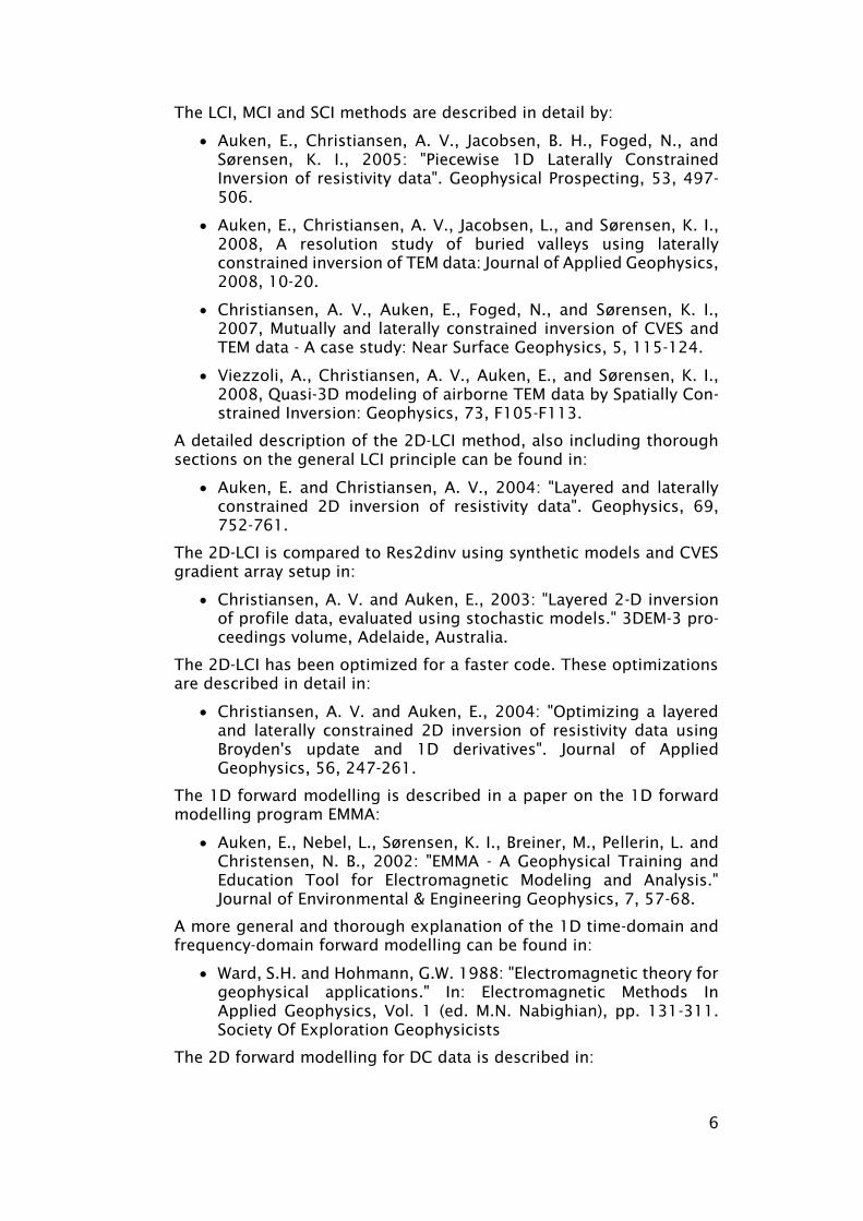
Model file with three data files (one TEM-file and two DCP-files)
(Figure 4.10). Lateral constrain between model 1 and model 2 as well
as between model 1 and model 3. No constraints between model 2
and 3.
23
# Text Comments
1 Model label - tem and resistivity data sets
2 3 3 !#DataFiles, Constraints mode (0->non, 1->Ver, >=2->Ver+Hor)
3 1 1 tem-file1.tem !ModelNr, ParameterLayout (1->res,thk,depth), data file name
4 2 1 dcp-file2.dcp !ModelNr, ParameterLayout (1->res,thk,depth), data file name
5 3 1 dcp-file3.dcp !ModelNr, ParameterLayout (1->res,thk,depth), data file name
6 50 !#Iterations
7 3 !#Layers, Model 1
8 30 -1 9e9 0.1 0.3 !Resistivity, priori STD, vert. constraints, horiz. constraints
9 100 -1 9e9 0.1 0.3
10 10 -1 0.1 0.3
11 20 -1 9e9 9e9 9e9 !Thickness, priori STD, vert. con., horiz. con-1, horiz. con-2
12 30 -1 99 99
13 20 -1 0.2 0.5 !Depth, prior STD, horiz. con.
14 50 -1 0.2 0.5
15 3 !#Layers, Model 2
16 30 -1 9e9 9e9 !Resistivity, a priori STD, vert. con.
17 100 -1 9e9 9e9
18 10 -1 9e9
19 20 -1 9e9 9e9 !Thickness, priori STD, vert. constraints, horiz. constraints
20 30 -1 9e9
21 20 -1 9e9 !Depth, prior STD
22 50 -1 9e9
23 3 !#Layers, Model 3
24 30 -1 9e9 !Resistivity, prior STD, vert. con.
25 100 -1 9e9
26 10 -1
27 20 -1 9e9 !Thickness, priori STD, vert. constraints.
28 30 -1
29 20 -1 !Depth, a priori STD
30 50 -1
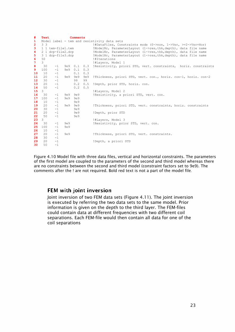
Figure 4.10 Model file with three data files, vertical and horizontal constraints. The parameters
of the first model are coupled to the parameters of the second and third model whereas there
are no constraints between the second and third model (constraint factors set to 9e9). The
comments after the ! are not required. Bold red text is not a part of the model file.
Joint inversion of two FEM data sets (Figure 4.11). The joint inversion
is executed by referring the two data sets to the same model. Prior
information is given on the depth to the third layer. The FEM-files
could contain data at different frequencies with two different coil
separations. Each FEM-file would then contain all data for one of the
coil separations

24
# Text Comments
1 Model label - two fem-data sets
2 2 0 !# of data files, Con. mode
3 1 1 fem-file1.fem
4 1 1 fem-file2.fem
5 50 !#Iterations
6 3 !#Layers, Model 1
7 30 -1 !Resistivity, priori STD
8 100 -1
9 10 -1
10 20 -1 !Thickness, priori STD
11 30 -1
12 20 -1 !Depth, prior STD
13 47 0.1
Figure 4.11 Model file with two fem-data files referring to the same model. The model has prior
on the depths to the second layer and no vertical and horizontal constraints. The comments
after the ! are not required. Bold red text is not a part of the model file.
Three data files (two FEM-files and one DCP file) and two models with
vertical and horizontal constraints (Figure 4.12). The two FEM-files uses
model definition 1 (line 7-14) and the DCP-files uses model definition
2 (line 15-22).
# Text Comments
1 Model label - two fem-data sets and one dcp-data set
2 3 2 !# of data files, Con. mode (verical and horizontal constraints)
3 1 1 fem-file.fem
4 1 1 fem-file.fem
5 2 1 dcp-file.dcp
6 50 !#Iterations
7 3 !#Layers, Model 1
8 30 -1 99 0.2 !Resistivity, priori STD, vert. constraints, horiz. constraints
9 100 -1 99 0.1
10 10 -1 0.1
11 20 -1 99 99 !Thickness, priori STD, vert. constraints, horiz. constraints
12 30 -1 99
13 20 -1 0.2 !Depth, priori STD, (no value), horiz. constraints
14 50 -1 0.2
15 3 !#Layers, Model 2
16 30 -1 99
17 100 0.1 99
18 10 -1
19 20 -1 99
20 30 -1
21 20 -1
22 50 -1
Figure 4.12 Model file with three data files, two models and vertical and horizontal constraints.
The two fem-files uses model definition 1 while the dcp-file use model definition 2. The
comments after the ! are not required. Bold red text is not a part of the model file

25
Model file for 2D-LCI inversion of 200 DC data sets (Figure 4.13).
# Text Comments
1 21.august.2003 14:13:57.57
2 200 2 !NDatafiles, NCoinstraint
3 1 2 LCI_0000.dcp !The "2" sets the model as DC 2D-LCI
4 2 2 LCI_0005.dcp
5 3 2 LCI_0010.dcp
6 .
7 .
8 198 2 LCI_0985.dcp
9 199 2 LCI_0990.dcp
10 200 2 LCI_0995.dcp
11 50 !Nite, 0=analyse
12 3 0 0 0 !#Layers, x, y, z of Model 1
13 121.0 -1 1.0e+010 1.4e-001 !Resistivity, prior, vert. constraints, horiz. constr.
14 121.0 -1 1.0e+010 1.2e-001
15 121.0 -1 1.0e-001
16 4.0 -1 1.0e+010 1.0e+010 !Thickness , prior, vert. constraints, horiz. constr.
17 8.0 -1 1.0e+010
18 4.0 -1 1.4e-001 !Depth , prior, , horiz. constr.
19 12.0 -1 1.0e-001
20 3 5 0 0 !#Layers, x, y, z of Model 2
21 121.0 -1 1.0e+010 1.4e-001
22 121.0 -1 1.0e+010 1.2e-001
23 121.0 -1 1.0e-001
24 4.0 -1 1.0e+010 1.0e+010
25 8.0 -1 1.0e+010
26 4.0 -1 1.4e-001
27 12.0 -1 1.0e-001
28 3 10 0 0 !#Layers, x, y, z of Model 3
29 121.0 -1 1.0e+010 1.4e-001
30 121.0 -1 1.0e+010 1.2e-001
31 121.0 -1 1.0e-001
32 4.0 -1 1.0e+010 1.0e+010
33 8.0 -1 1.0e+010
34 4.0 -1 1.4e-001
35 12.0 -1 1.0e-001
36 .
37 .
38 3 985 0 0
39 121.0 -1 1.0e+010 1.4e-001
40 121.0 -1 1.0e+010 1.2e-001
41 121.0 -1 1.0e-001
42 4.0 -1 1.0e+010 1.0e+010
43 8.0 -1 1.0e+010
44 4.0 -1 1.4e-001
45 12.0 -1 1.0e-001
46 3 990 0 0
47 121.0 -1 1.0e+010 1.4e-001
48 121.0 -1 1.0e+010 1.2e-001
49 121.0 -1 1.0e-001
50 4.0 -1 1.0e+010 1.0e+010
51 8.0 -1 1.0e+010
52 4.0 -1 1.4e-001
53 12.0 -1 1.0e-001
54 3 995 0 0
55 121.0 -1 1.0e+010 1.4e-001
56 121.0 -1 1.0e+010 1.2e-001
57 121.0 -1 1.0e-001
58 4.0 -1 1.0e+010 1.0e+010
59 8.0 -1 1.0e+010
60 4.0 -1 1.4e-001
61 12.0 -1 1.0e-001
Figure 4.13 Model file for 2D-LCI inversion of DC data. Constraints are applied on resistivities and
depths. The comments after the ! are not required. Bold red text is not a part of the model file

26
For TEM data there is an option to model for the geometry and
parameters of a thin sheet. In this case there is just one model/sheet,
but multiple data files all optimizing the same model.
The parameters that we invert for are: sheet conductance, sheet
positions (x,y,z) referring to the top-center of the sheet, sheet width,
sheet height, strike angle and dip angle. An example is shown in Figure
4.14.
# Text Comments
1 Model file for sheets modelling
2 5 1
3 1 10 z1.tem
4 1 10 x1.tem
5 1 10 z2.tem
6 1 10 x2.tem
7 1 10 z3.tem
8 50
9 2 1 !#Layer, #sheets
10 10.92 0.50 !Sheet conductance = thickness*conductiivty
11 142.92 0.50 !Sheet x-position - center of sheet
12 343.92 0.50 !Sheet y-position - center of sheet
13 24.92 0.50 !Sheet z-position - top - center of sheet
14 45.92 0.50 !Sheet width
15 46.92 0.50 !Sheet height
16 47.92 0.50 !Strike angle
17 48.92 0.50 !Dip
18 30.00 -1.00 1.0000 !Res 1, Background Model
19 10.00 -1.00 !Res 2
20 20.00 -1.00 !Thk 1
21 20.00 -1.00 !Dph 1
Figure 4.14 Model file for sheet inversion using airborne TEM data. x and a z-datafiles work on the
same model. The comments after the ! are not required. Bold red text is not a part of the model file.
For 1D layered inversion of surface wave dispersion (swd) curves there
are just one model format, but the interpretation can be one of two.
The file format always includes velocity, density, Poisson’s ratio,
thicknesses and depths the layers as shown in Figure 4.15.
The two ways of using the swd model format are controlled by the
second integer on the line with the filenames as described in section
4.1 “ Heading part”.

27
The formatting of the non-general parts of these special cases are
described below.
In the case of airborne EM measurements, the transmitter altitude can
be included as an inversion parameter. A model file intended for that
purpose is shown in Figure 4.16.
The altitude parameter is included as an extra line in the file model
format, everything else is the same. The altitude is given as a positive
number.
Lateral constraints and a priori constraints are applied as usual.
# Text Comments
1 Model label
2 2 2 !# of data files, Con. mode (vertical and lateral constraints)
3 1 3 swd-file1.swd
4 1 3 swd-file2.swd
5 50 !#Iterations
5 3 !#Layers, Model 1
6 700 -1 1e9 0.2 !Velocity, priori STD, vertical constraints, lateral constraints.
7 700 -1 1e9 0.2
8 700 -1 0.2
9 2000 1e-3 1e9 1e9 !Density, priori STD, vertical constraints, lateral constraints.
10 2000 1e-3 1e9 1e9
11 2000 1e-3 1e9
12 0.4 1e-3 1e9 1e9 !Poissons ratio, priori STD, vertical constraints, lateral constraints.
13 0.4 1e-3 1e9 1e9
14 0.4 1e-3 1e9
15 2 -1 1e9 1e9 !Thickness, priori STD, vertical constraints, lateral constraints.
16 2 -1 1e9
17 2 -1 0.1 !Depth, priori STD, lateral constraints.
18 4 -1 0.1
19 3 !#Layers, Model 2 (must be the same as model 1 with lateral constraints)
20 700 -1 1e9 0.2 !Velocity, priori STD, vertical constraints, lateral constraints.
21 700 -1 1e9 0.2
22 700 -1 0.2
23 2000 1e-3 1e9 1e9 !Density, priori STD, vertical constraints, lateral constraints.
24 2000 1e-3 1e9 1e9
25 2000 1e-3 1e9
26 0.4 1e-3 1e9 1e9 !Poissons ratio, priori STD, vertical constraints, lateral constraints.
27 0.4 1e-3 1e9 1e9
28 0.4 1e-3 1e9
29 2 -1 1e9 1e9 !Thickness, priori STD, vertical constraints, lateral constraints.
30 2 -1 1e9
31 2 -1 0.1 !Depth, priori STD, lateral constraints.
32 4 -1 0.1
Figure 4.15 Model file for surface wave dispersion curve modelling. In this case two data-files are
connected with lateral constraints. The comments after the ! are not required. Bold red text is not a
part of the data file.

28
# Text Comments
1 Model label - one model
2 1 0 !# of data files, Con. mode
3 1 5 tem-airborne-file.tem
4 50 !# of iterations
5 3 !# of layers, model 1
6 15 0.05 !transmitter altitude, transmitter altitude prior_STD
7 30 -1 !Resistivity_1, Resistivity_1 prior_STD
8 100 -1 !Resistivity_2, Resistivity_2 prior_STD
9 10 -1 !Resistivity_3, Resistivity_3 prior_STD
10 20 -1 !Thickness_1,Thickness_1 STD
11 30 -1 !Thickness_2,Thickness_2 STD
12 20 -1 !Depth_1, Depth_1 STD
13 47 -1 !Depth_2, Depth_2 STD
Figure 4.16 Model file for EM inversion with an altitude parameter. The comments after the ! are not
required. Bold red text is not a part of the model file.
If working with x-component airborne TEM data, the x-receiver tilt-
angle can be included as an inversion parameter together with the
altitude. The x-receiver is fixed to the Tx frame (SkyTEM type). A model
file intended for that purpose is shown in Figure 4.17.
The angle parameter is included as an extra line in the file model
format just after the altitude parameter, everything else is the same.
It is not possible to apply lateral constraints on the angle parameter,
but an a priori constraint can be applied.
The angle is defined in the positive direction for a right-handed coordi-
nate system with the z-axis pointing downwards. Thus, 270 degrees is
vertical, a larger angle is when the x-receiver tilts in the positive x-
direction and vice versa. The x-receiver plane is assumed to be
perpendicular to the z-transmitter plane.
# Text Comments
1 Model label - one model
2 1 0 !# of data files, Con. mode
3 1 6 tem-airborne-file.tem
4 50 !# of iterations
5 3 !# of layers, model 1
6 15 0.05 !transmitter altitude, transmitter altitude prior_STD
7 272 0.01 !transmitter angle, transmitter angle prior_STD
8 30 -1 !Resistivity_1, Resistivity_1 prior_STD
9 100 -1 !Resistivity_2, Resistivity_2 prior_STD
10 10 -1 !Resistivity_3, Resistivity_3 prior_STD
11 20 -1 !Thickness_1,Thickness_1 STD
12 30 -1 !Thickness_2,Thickness_2 STD
13 20 -1 !Depth_1, Depth_1 STD
14 47 -1 !Depth_2, Depth_2 STD
Figure 4.17 Model file for EM inversion with both an altitude parameter and an transmitter angle
parameter. The comments after the ! are not required. Bold red text is not a part of the model file

29
For HEM you can invert for altitude and electrical permittivity of layers
together with the ordinary layer parameters (resistivities, thicknesses
and depths).
The altitude parameter is included as an extra line in the file model
format as a positive number.
Lateral constraints and a priori constraints are applied as usual.
The electrical permittivities of layers are added similar to resistivities
of layers. A model file intended for this purpose is shown in Figure
4.18.
# Text Comments
1 Model label - one model
2 1 0 !# of data files, Con. mode
3 1 7 hem-airborne-file.hem
4 50 !#Iterations
5 3 !#Layers, Model 1
6 45 0.05 !transmitter altitude, transmitter altitude prior_STD
7 30 -1 !Resistivity_1, Resistivity_1 prior_STD
8 100 -1 !Resistivity_2, Resistivity_2 prior_STD
9 10 -1 !Resistivity_3, Resistivity_3 prior_STD
7 7e-11 -1 !Permitivity_1, Permitivity_1 prior_STD
8 3e-11 -1 !Permitivity_2, Permitivity_2 prior_STD
9 4e-11 -1 !Permitivity_3, Permitivity_3 prior_STD
10 20 -1 !Thickness_1,Thickness_1 STD
11 30 -1 !Thickness_2,Thickness_2 STD
12 20 -1 !Depth_1, Depth_1 STD
13 47 -1 !Depth_2, Depth_2 STD
Figure 4.18 Model file for EM inversion with an altitude parameter and electrical permitivity of layers.
The comments after the ! are not required. Bold red text is not a part of the model file.
In the case of an airborne towed bird TEM system that measures at
least the x and z-component we can invert for bird geometry as well.
The geometrical parameters that we invert for are Tx, altitude, angle
between Tx and Rx, distance between Tx and Rx, Rx pitch angle and
Rx roll angle. The geometry parameters inverted for are all shown in
Figure 4.19. An example model file is shown in Figure 4.20.

30
Figure 4.19. Overview of geometry parameters that can be inverted for
when using the general towed bird TEM format.
# Text Comments
1 Model file for two data files working to optimize the same model
2 2 1
3 1 8 x.tem
4 1 8 z.tem
5 50
6 3
7 120.6 -1 0.3 !TxAlt
8 201.0 -1 0.05 !Theta, angle between Tx and Rx, 180 nominal
9 70.0 -1 0.05 !DTxRx, distance between Tx and Rx [m]
10 181.0 -1 0.3 !Alfa_Pitch, 180 nominal
11 175.0 -1 0.3 !Alfa_Roll, 180 nominal
12 30.0 -1 9e9 0.3 !Res_1
13 40.0 -1 9e9 0.3 !Res_2
14 10.0 -1 0.3 !Res_3
15 20.0 -1 9e9 1.4 !Thk_1
16 20.0 -1 1.6 !Thk_2
17 20.0 -1 1.7 !Dph_1
18 40.0 -1 1.9 !Dph_2
Figure 4.20 Model file for airborne TEM inversion with an towed bird and inversion for geometry
parameters for the bird. A x and and a z-datafile work on the same model. The comments after the !
are not required. Bold red text is not a part of the model file.
For airborne TEM data it is possible to include a shift factor as an extra
inversion parameter on top of the transmitter altitude. The shift factor

31
is simply multiplied to all of the measured data. A model file for that
purpose is shown in Figure 4.21.
# Text Comments
1 Model label - one model
2 1 0 !# of data files, Con. mode
3 1 51 tem-airborne-file.tem
4 50 !# of iterations
5 3 !# of layers, model 1
6 15 0.05 !transmitter altitude, transmitter altitude prior_STD
7 1.1 0.05 !shift factor, shift factor prior_STD
8 30 -1 !Resistivity_1, Resistivity_1 prior_STD
9 100 -1 !Resistivity_2, Resistivity_2 prior_STD
10 10 -1 !Resistivity_3, Resistivity_3 prior_STD
11 20 -1 !Thickness_1,Thickness_1 STD
12 30 -1 !Thickness_2,Thickness_2 STD
13 20 -1 !Depth_1, Depth_1 STD
14 47 -1 !Depth_2, Depth_2 STD
Figure 4.21 Model file for TEM inversion with an altitude parameter and a shift factor. The comments
after the ! are not required. Bold red text is not a part of the model file.
For early times of airborne TEM data it is possible to consider an
additional CR or system response. This CR is a small primary field due
to residual current in the transmitter loop at early times and is usually
measured at high altitude. It is important to note that the CR shape has
to be stable (which is the case for SkyTEM system) in order to
compensate it correctly! If not, removal of early times remains the best
solution.
Studies with SkyTEM system have shown that if CR shape is stable, its
amplitude is not and varies because of few cm bending of the frame
during flight. It is thus necessary to consider a scaling factor which is
evaluated as an inversion parameter.
Figure 4.22 shows an example of *.mod file using the CR correction for
the inversion. Note the differences:
- Type on line 3 is now 52.
- The CR scaling factor and its prior STD on line 7: the starting
value is normally equal to 1. Note that, because this factor
needs to be able to change sign, the convention is to write it
in the *.mod file with a shift of +100. So a starting value of
1 is actually written as 101. The prior STD can be left quite
loose, the most important thing being to set the lateral
constraint on the CR scaling factor relatively tight along a
flight line.
Parallel to the *.mod file you need to have in the same folder a *.bia
file which is a basic ascii file which has the same name as the *.mod
file, but with a different file extension. Figure 4.23 shows an example
of such a *.bia file. Important things you should be aware of regarding
the numbers in the *.bia file:

32
- Check that the center gate times (1st
column in *.bia file)
to the ones written in the tem files (with
Aarhus Workbench the timing in *.geo file + calibration time
shift)
- The unit of the db/dt response of the CR (2nd
column in *.bia
file). It has to be normalized by the current and the number
of wire turns, but not by the area of the transmitter loop. In
fact, it is the unit convention in *.tem files, since the shape
and area of the transmitter loop are considered in the
modeling of the response.
You can put as many gates as you want in the *.bia file, even if the CR
becomes very low in the last lines, it will simply have no impact.
# Text Comments
1 Model file example with coil response (CR) correction
2 1 0
3 1 52 tem-airborne-file.tem
4 0
5 3 !#Layers, Model 1
6 3.6841e+01 0.05 !Transmitter altitude, transmitter altitude prior_STD
7 101 1.0007e+00 !CR scaling factor, CR scaling factor prior_STD
8 30 -1 !Resistivity_1, Resistivity_1 prior_STD
9 100 -1 !Resistivity_2, Resistivity_2 prior_STD
10 10 -1 !Resistivity_3, Resistivity_3 prior_STD
11 20 -1 !Thickness_1,Thickness_1 STD
12 30 -1 !Thickness_2,Thickness_2 STD
13 20 -1 !Depth_1, Depth_1 STD
14 47 -1 !Depth_2, Depth_2 STD
Figure 4.22 Model file for TEM inversion with altitude parameter and bias/coil response correction.
The comments after the ! are not required. Bold red text is not a part of the data file.
# Text Comments
1 Example of *.bia file for Coil Response (CR) correction
2 0.0200000E-06 2.0869769E-07 !center gate time (s), db/dt value of CR (V/(m²x A x N))
3 2.0200000E-06 -4.8598424E-05
4 4.0200000E-06 -1.8183371E-05
5 6.0200000E-06 -2.5425268E-06
6 8.0200000E-06 -2.9445568E-07
7 10.0200000E-06 -2.2408661E-08
Figure 4.23 *.bia file for TEM inversion with altitude parameter and bias/coil response correction.
The comments after the ! are not required. Bold red text is not a part of the data file.

33
The con-file controls various settings in the inversion procedure.
AarhusInv is compatible with three configuration file versions: Version
15, version 20, and version 21.
Version 15 is an outdated version and is not described here. However,
file examples can be downloaded from the web page. In the outdated
versions all parameters must be specified in the con files. In version 20
and onwards, only the parameters that do not take the default values
are specified. All specified parameters and default values can be
printed out by typing “AarhusInv.exe help”. The parameters are also
printed in the log-file.
Here only version 20 will be described and an example is shown in
Figure 5.1. The parameters specified in this example, are the
parameters that can be changed by all users. Each parameter is
explained in the following section.
Parameters, which should only be changed by expert users, are
described in sections 5.2 - 5.14.
On the webpage you will find two con-file examples: One with the
parameters which can be changed by all users (similar to Figure 5.1)
and one with all the expert-user parameters.
# Text Comments
1 Confile settings: %Text string
2 20 %con file version
3 %In/output settings
4 OutputGen = 0 %0 -> general information to screen, 1 -> to file
5 OutputLog = 0 %0 -> overwrite log file, 1 -> append
6 OutputCov = 0 %1 -> write J, rough. and cov. matrices on .emm file, 0 -> don't
7 EmoWriteIte = 0 %1 -> write emo-type file after each ite. (.ems), 0 -> don't
8 %Inversion settings
9 NCPUs = 1 %Number of CPUs used
10 CalcAnalysis = 1 %0 -> Don’t Calc.; 1 -> Coup. anal.; 2 -> Coup. and uncoup. anal.
11 %Model linear/log settings
12 LogModel = 0 %0 -> Inversion in log model space, 1 -> lin
13 LogData = 0 %0 -> Inversion in log data space, 1 -> lin
14 LogNeg = 0 %0 -> Warn for negative data, but continue inv; 1 -> Stop when
negative; 2 -> Change to lin space when negative
15 LogDepth = 0 %0 -> Rel. depth const., inv. in log space, 1 -> Abs. depth const.
16 DepthRef = 1 %0 -> Depth-ref. lateral const.,1 -> Elevation-ref. lateral const.
17 AltRef = 0 %0 -> Height ref. Tx-altitudes, 1 -> Elevation ref. Tx-altitudes
18 %Parameter settings
19 MinRes = 1.00E-01 %Min resistivity (ohmm) allowed
20 MaxRes = 2.00E+04 %Max resistivity (ohmm) allowed
21 MinThick = 1.00E-01 %Min thicknes (m) allowed
22 MaxThick = 5.00E+02 %Max thicknes (m) allowed
23 %Forward settings
24 AddNoise2Scr = 0 %0 -> add noise to forward (.fwr) files, 1 -> no noise
Figure 5.1. Example of con-file version 20, where only a subset of parameters are specified. All
parameters not listed take the default value. Lines starting with % are for comments and everything
after % are comments as well.

34
The con-file has two mandatory lines in the beginning where the first
is a comment and the second is the CON-file version. For all other lines
the following apply:
Format: [parameter_name] = value
Lines starting with “%” are comments
After any values, optional comments can be added by writing a
“%” followed by the comment.
The following parameters can be changed by all users. The numbering
refers to Figure 5.1.
This section controls where and what to be written from the inversion
output.
Value 0: General information will be written to screen.
Value 1: General information will be written to files.
Value 0: Overwrite the log file between subsequent runs of
AarhusInv.
Value 1: The log file is appended between subsequent runs.
Value 1: The covariance matrix, Jacobian matrix and roughness
matrix will be written in the emm-file.
Value 0: No matrices written.
Value 1: Write emo-type file after each iteration (.ems).
Value 0: Do not write.
Numbers of CPUs used.
Value 0: Do not calculate.
Value 1: Calculate coupled analysis only.
Value 2: Calculate coupled and un-coupled analyses
This section control weather the computations are performed in linear
or log space.

35
Value 0: Inversion in log model space
Value 1: Inversion in linear model space
Value 0: Inversion in log data space
Value 1: Inversion in linear data space
All settings refer to the case when LogData=0
Value 0: Warn for negative forward data, but continue the
inversion by taking the absolute values of negative forward data.
Value 1: Stop when negative forward data are encountered.
Value 2: Change to linear data space when negative forward data
are found.
Value 0: Relative depth constraints (default).
Value 1: Absolute depth constraints.
Value 0: Depth referenced model.
Value 1: Elevation referenced model (default).
Value 0: Height referenced altitudes.
Value 1: Elevation referenced altitudes (default).
Here the dynamic range of the model parameters is set.
These lines set the range on the thickness and the resistivity in the
inversion.
The total list of parameter maximum and minimum limits that can be
specified in the con-file can always be listed typing “AarhusInv.exe
help”. The list includes:
MinRes, MaxRes: resistivity [ohmm].
MinThick, MaxThick: thickness [m].
MinImagSigma, MaxImagSigma: imaginary conductivity
(MIC/BIC/CCPA IP model) [mS/m]
MaxM0, MinM0: M0 (RCC/CCC IP model) [mV/V].
MaxTau, MinTau: Tau (RCC/CCC/MPA/MIC/BIC/TBIC/CCeps IP
models) [s].
MaxC, MinC: C (RCC/CCC/MPA/MIC/BIC/TBIC/CCeps IP models)
[dim-less].

36
MaxPhi, MinPhi: Phi (CPA/Drake/MPA IP models) [mrad].
MaxfL, MinfL: fL (Drake IP model) [mHz].
MinW, MaxW: W (MRS) [m3
/m3
]
MinT2Star, MaxT2Star: Tau (MRS) [s].
MinCmrs, MaxCmrs: C (MRS) [dimless].
MinShift, MaxShift : shift (MRS) [rad] .
MaxEps, MinEps: relative Permittivity (CCeps IP model) [dimless].
MaxTemp, MinTemp: temperature (TRES/TBIC DC/IP models)
[Celsius].
Besides these limits a few additional parameter settings can be defined:
RefTemp: reference temperature (TRES/TBIC DC/IP models)
[Celsius] for conductivity-temperature dependence.
dSigma/dTemp: slope for DC conductivity-temperature
(TRES/TBIC DC/IP models) [S/m/Celsius] dependence.
dSigma2nd/dTemp: slope for imaginary conductivity-tempe-
rature dependence (TBIC IP model) [S/m/Celsius].
Sigma2ndSurf/Sigma1stSurf: proportionality between real and
imaginary surface conductivity at peak frequency (BIC/TBIC IP
models) [dimless]
Value 1: White noise is added to the forward response in the fwr-
files with the STD as specified in the data files.
Value 0: No noise is added to the forward response.
The following settings should be changed by expert users only.
Parameters with no prior information are assigned MinApriori as STD.
Should not be changed.
The initial maximum parameter change. If MaxStep is exceeded, the
damping continues.
The overall minimum allowed parameter change.
The factor to increase the MaxStep after a successful iteration.
The factor to decrease MaxStep if the norm increases.

37
Number of iterations between increments of MaxStep.
Value 1: Reuse G from the last iteration for the analysis.
Value 0: Recalculate G from final result.
Integer indicating the number of close neighbours used in the analysis.
Value 0: Parallel sparse analysis for the full problem.
Value 1: Coupled to nearest neighbours.
Value 2: Further coupled to two nearest neighbours.
Value -1: Parallel sparse analysis for the full problem
(NPar<1000) or coupled to nearest neighbours (NPar>1000).
Solver type in the solution of the linear problem.
Value 0: Sparse solver (except for 2D DCIP and MRS)
Value 1: Dense solver and Dense algebra.
Value 11: SSOR
Value 12: LU0
Value 13: LUT
Value 14: BLUT
Value 15: A-Phi solver for 3D TEM
Value -1: Auto-selected sparse solver or dense solver for 2D DCIP
and MRS
Relative change in total norm (residual) to stop iterations for single-
side derivatives.
Relative change in total norm (residual) to stop iterations for double-
side derivatives.
Relative change in norm to stop iterations on any subset of size
SubsetNormChangeSize.
Relative size of model space where the stop criterion must obey
RelSubsetNormChange regardless of RelNormChangeD or
RelNormChange
Numbers of iterations before setting the altitude free in the inversion.
(Only model types 5 and 6).

38
Numbers of iterations before setting the angle free in the inversion.
(Only model type 6).
Value 1: Broyden’s update is used in the calculation of deriva-
tives.
Value 0: Broyden’s update is not used.
The number of full 2D iterations to be performed to initialize the
Jacobian matrix before switching to Broyden’s update (only if
Broyden=1). This value must be 1 if Broyden’s update is used with
2D-DC computations.
Relative change in norm before recalculating the Jacobian matrix (only
if Broyden=1). To use Broyden’s update, RelNormChangeB must be
larger than RelNormChange. Otherwise the iterations stop before start-
ing to use Broyden’s update.
Number of iterations in which derivatives are using approximate
responses for the derivatives in the Jacobian.
For TEM it is the Fast Approximate Inversion (FAI) being used:
Only segmented (type 72) and square (type 7) loops are
supported.
You can have only one Tx loop geometry for each single dataset.
It works for all magnetic components, X, Y and Z.
The initialization can last more than 20 s on a dataset with
several altitudes, however it is fast when computing forward
response with one altitude only or when inverting TEM data
without altitude as an inversion parameter.
Number iterations with approximate forward computation. (Model type
specific). IMPORTANT: for TEM a value larger than 0 will introduce a
strong approximation in the calculations.
Value 1: Always end with accurate (non-approximate) iterations
(switch back if last iteration was using approximation)
Value 0: Do not.
Value 1: Always end with minimum step size.
Value 0: Do not.

39
This section controls the setting used for computation the depth of
investigation (DOI). The following parameters should be changed by
expert users only.
For more information on the DOI see section 15.4: “Depth of
Investigation”.
Value 1: Calculate DOI. For Nite=0 in the mod-file, the
calculations are done for the input model.
Value 0: Do not calculate DOI.
Number of layers for the DOI calculations.
Thickness of the first layer used in the DOI calculations.
Depth the last layer boundary used in the DOI calculations.
High absolute threshold value for the DOI (shallow).
Low absolute threshold value for the DOI (deep).
High relative threshold value for the DOI (shallow).
Low relative threshold value for the DOI (deep).
High CAA (Cumulated Approximate Analysis) value for the DOI
(shallow).
Low CAA (Cumulated Approximate Analysis) value for the DOI (deep).
The following parameters should be changed by expert users only.
Initial damping, 1st iteration: Max(diagonal)/DampInit.
Maximum value of DampInit. If a value larger than MaxDampInit is
found, it is set to MaxDampInit.
Factor to increase DampInit after a successful iteration.

40
Factor to increase the damping of the diagonal elements if previous
damping was not sufficient.
Maximum number of damping steps before giving up.
First damping value.
Value 1: No damping on the parameters driven only by
constrains (with no Jacobian entries).
Value 0: Damping on all parameters.
Value 1: True. Different damping for each parameter type.
Value 0: False. Same damping value for all parameter types.
The following settings should be changed by expert users only.
Low filter density for the cos-sine filter. (Forward responses use a filter
density of FDenseCSHigh whereas derivatives are calculated with a
density of FDenseCSLow.)
High filter density for the cos-sine filter.
Low filter density for the J_1-J1 filter.
High filter density for the J_1-J1 filter.
The coarsest temporal sampling used for the system response convo-
lution.
Refinement samplings steps used for the system response convolution.
Finest sampling is 2^SRConvNSamplingSteps
*SRConvCoarsestSampling.
Refinelimit which determines when to calculate more points. If a
straight line approximation is more than SRConvRefinementLimit off,
refinement is performed.

41
The coarsest temporal sampling used for the time domain filter convo-
lution.
Refinement samplings steps used for the the time domain filter
convolution. Finest sampling is 2^TDFiltConvNSamplingSteps
*TDFiltConvCoarsestSamp.
Refinement limit for time domain filter convolution.
The following settings should be changed by expert users only.
Number of different transmitter altitudes.
Number of reference conductivities.
Reference resistivities.
This section describes the settings used for 2D DC/IP inversions. The
following parameters should be changed by expert users only.
Lower decade for the allocation of the Frequency Domain 2D DCIP
Kernels. (Default value is -8)
Upper decade for the allocation of the Frequency Domain 2D DCIP
Kernels. (Default value is 4).
Indicates what to do when the frequency range is exceeded:
Value 0: Stop the inversion.
Value 1: Warn and extend range at next iteration.
Value 2: Warn but keep the .con range

42
Number of points per decade for kernel splining in low resolution mode
(only when the iteration number NIte<=NApproxFor).
Number of points per decade for kernel splining in high resolution
mode (only when the iteration number NIte>NApproxFor.).
Number of neighbouring models to the data point for the computation
of the 2D Jacobian in low resolution mode.
Number of neighbouring models to the data point for the computation
of the 2D Jacobian in high resolution mode.
Value 1: The minimum between DC total norm (residual) and IP
total norm (residual) is considered as stopping criteria (in low
resolution mode).
Value 0: The global (DC+IP) norm is used.
Value 1: The minimum between DC total norm (residual) and IP
total norm (residual) is considered as stopping criteria (in high
resolution mode).
Value 0: The global (DC+IP) norm is used
Multiplicative scaling factor for IP data/model STDs, in low resolution
mode (it balances the DC versus IP Jacobian/Constraints). When
IPFactor>100, the IP Jacobian computation is turned off
Multiplicative scaling factor for IP data/model STDs, in high resolution
mode (it balances the DC versus IP Jacobian/Constraints). When
IPFactor>100, the IP Jacobian computation is turned off.
This section the settings used for SWD computations. The following
parameters should be changed by expert users only.
Value 0: All layers are solid.
Value 1: With liquid top layer.
Max step in wavenumber search for SWD forward calculations (default
2e-5).

43
In this section, the settings for surface NMR/MRS are described. The
following parameters should be changed by expert users only.
Min Z discretization limit, expressed as depth value [m].
Max Z discretization limit, expressed as number of loop side lengths.
Min horizontal discretization limit, expressed as fraction of loop side
length.
Max horizontal discretization limit, expressed as fraction of loop side
length.
Depth [m] at which z discretization (number of samples) is changed.
Expressed as fraction of loop side length.
Number of points per decade for the Z discretization (Shallow setting).
Number of points per decade for the Z discretization (Deep setting).
Horizontal discretization, number of discretization points between wire
and the center (to the next wire), shallow discretization.
Horizontal discretization, number of discretization points between wire
and the center (to the next wire), deep discretization.
Minimum number of discretization points in each layer.
Value 1: Print out XYZ discretization, magnetic fields, tip angles,
3D/1D/integrated kernels.
Value 0: Do not print.
q number for which tip angle is printed.
In this section, the settings for 2D HEM are described. The following
parameters should be changed by expert users only.

44
Max number of models for forward sectioning.
Max number of models for derivative sectioning.
Number of neighbouring soundings included in the Jacobian matrix
Number of soundings to overlap
In this section, the settings for voxel computations are described. The
following parameters should be changed by expert users only. This
part is under development!
Number of norms to be excluded for un-connected nodes (i.e. model
nodes not connected to any forward node).
Number of norms to be changed for un-connected nodes (i.e. model
nodes not connected to any forward node).
Norm indexes to be excluded, one number for each NExcludedNorms.
Norm indexes to be changed (:,1)=old, (:,2)=new, for each
NChangedNorms.
Value 1: Write model/constraint meshes including nodes far
from flight lines to a file.
Value 0: Do not write.
Value 1: Export model, forward model and data in a Aarhus
Workbench compatible format.
Value 0: Do not.
Value 1: Write constraint mesh to file.
Value 0: Do not.
Value 1: Write forward mesh to file.
Value 0: Do not.

45
Dummy value for un-connected nodes in the workbench-style mesh
export.
In this section, the setting for Markov chain Monte Carlo (MCMC)
computations are described. The following parameters should be
changed by expert users only.
Value 0: No MCMC. (default)
Value 1: MCMC with uniform proposer.
Value 2: MCMC with sensitivity matrix-based proposer.
Factor for scaling the step length of the model perturbation. Should be
tuned to give an acceptance rate around 20-30%.
Maximum relative weight to proposing steps for uncertain parameters.
(i.e. N times larger than the best determined).
Number of steps between updating the sensitivity matrix in the propo-
ser. Used only for MCMCType=2.
Number of proposes/iterations to run.
In this section, the settings for BFGS solver computations are
described. The following parameters should be changed by expert
users only.
Number of derivatives stored in the BFGS routine.
Initial step length used in the BFGS.
Tolerance of model vector in BFGS.
Tolerance of objective function in BFGS.
Line search parameter delta for Wolfe conditions.

46
Line search parameter sigma for Wolfe conditions.
Line search parameters (tau) for Wolfe conditions - step lengths.
Value 1: Uses the adjoint state method for calculating the
derivative of the objective function.
Value 0: Uses the Jacobian.
In this section, the setting for parallelization are described. The
following parameters should be changed by expert users only. This
part is under development.
Mode of threads binding to cores:
Value 0: Shared mode.
Value 1: Dedicated mode.
Value 2: Manual mode.
Value 1: nested parallelization, typically only used for NUMA
architecture
Number of CPUs to use in outer parallelization, if set to 0 or negative
numbers, it will be set automatically in InitOpenMP.
Number of CPUs to use in inner parallelization, if UseNested=.false.
then NCPUInner=1.
The number of XeonPhis available.
Number of threads used on each XeonPhi.
Lower limit of CPUs to use in regions of the code which are memory
bandwidth limited in order to not oversaturate these regions.
Number of CPUs in regions with memory saturation in order to not
oversaturate the system.
Value 1: Distribute across different NUMA nodes.
Value 0: Keep on NUMA node until full

47
Thread to start the parallelization from:
Value -1: It selects a random one
Value > 0: Thread number

48
The TEM data input file contains transmitter geometry and waveform
settings along with the low pass filters of the TEM receiver and the
data.
The TEM-file is a flexible way of storing the measured data. The
settings in the TEM-file are used in the calculation of the forward
response in the AarhusInv code. An example of a TEM data file for a
central loop configuration sounding is shown in Figure 6.1.
Advanced settings regarding modelling with an arbitrary segmented
loop and the use of a transmitter front gate is described in section 6.2-
“Header lines with segmented loop and front gate”.
# Text Comments
1 Created by Emma
2 7 3 !SourceType, Field Polar (Hx=1....Ez=6)
3 0.0 0.0 0.0 0.0 0.0 0.0 !Tx X, Y, Z, Rx X, Y, Z
4 40.0 40.0 !Tx LoopSide X and Y
5 4 4 4 !Inp/out: Inp, Out, Inv (0->H,1->dH/dt,2->B,3->dB/dt,4->rhoa
6 3 3 !WaveFormType: 0->step,1->imp.,3->user def. d/dt,NWaveForms
7 3 -1.05E-03 -9.30E-04 0.00 1.00 -9.30E-04 0.00E+00 1.00 1.00 0.00E+00 2.50E-06 1.00 0.00
!Num. of Sub WF, T0,T1,A0,A1..
8 3 -4.00E-03 -3.88E-03 0.00 1.00 -3.88E-03 0.00E+00 1.00 1.00 0.00E+00 2.50E-06 1.00 0.00
!Num. of Sub WF, T0,T1,A0,A1..
9 3 -1.00E-02 -9.88E-03 0.00 1.00 -9.88E-03 0.00E+00 1.00 1.00 0.00E+00 2.50E-06 1.00 0.00
!Num. of Sub WF, T0,T1,A0,A1..
10 3 0 0 !NFilters, 1 modelling of FrontGate, Damping fact of primary field
11 1 1 2.40E+05 !LP/HP: NCutOff (0->no filter), FOrder(1,NCutOff),
FCutOff(1,NCutOff) (Hz)
12 0 !LP/HP: NCutOff (0->no filter), FOrder(1,NCutOff),
FCutOff(1,NCutOff) (Hz)
13 1 1 2.40E+05 !LP/HP: NCutOff (0->no filter), FOrder(1,NCutOff),
FCutOff(1,NCutOff) (Hz)
14 0 !LP/HP: NCutOff (0->no filter), FOrder(1,NCutOff),
FCutOff(1,NCutOff) (Hz)
15 1 1 3.70E+04 !LP/HP: NCutOff (0->no filter), FOrder(1,NCutOff),
FCutOff(1,NCutOff) (Hz)
16 0 !LP/HP: NCutOff (0->no filter), FOrder(1,NCutOff),
FCutOff(1,NCutOff) (Hz)
17 9.150E-06 2.769E+01 5.00E-02 1 1
18 1.152E-05 2.807E+01 5.00E-02 1 1
19 1.450E-05 2.823E+01 5.00E-02 1 1
10 1.826E-05 2.832E+01 5.00E-02 1 1
11 2.298E-05 2.849E+01 5.00E-02 1 1
12 2.893E-05 2.889E+01 5.00E-02 1 1
13 3.643E-05 2.964E+01 5.00E-02 1 1
14 4.586E-05 3.079E+01 5.00E-02 1 1
15 5.773E-05 3.243E+01 5.00E-02 1 1
16 7.268E-05 3.462E+01 5.00E-02 1 1
17 9.150E-05 3.722E+01 5.00E-02 1 1
18 1.152E-04 4.023E+01 5.00E-02 1 1
19 1.450E-04 4.311E+01 5.00E-02 1 1
20 1.826E-04 4.528E+01 5.00E-02 1 1
21 2.298E-04 4.621E+01 5.00E-02 1 1
22 2.894E-04 4.567E+01 5.00E-02 1 1
23 3.643E-04 4.375E+01 5.00E-02 1 1
24 4.586E-04 4.140E+01 5.00E-02 1 1
25 5.773E-04 3.884E+01 5.00E-02 1 1
26 7.268E-04 3.654E+01 5.00E-02 1 1
27 4.830E-05 3.109E+01 5.00E-02 2 2
28 6.081E-05 3.289E+01 5.00E-02 2 2
29 7.655E-05 3.508E+01 5.00E-02 2 2
30 9.637E-05 3.782E+01 5.00E-02 2 2
31 1.213E-04 4.070E+01 5.00E-02 2 2
32 . . . . .
33 . . . . .
34 1.923E-03 2.342E+01 5.00E-02 2 2
35 2.421E-03 2.228E+01 5.00E-02 2 2

49
36 1.000E-04 3.523E+01 5.00E-02 3 3
37 1.259E-04 3.862E+01 5.00E-02 3 3
38 1.585E-04 4.159E+01 5.00E-02 3 3
39 1.995E-04 4.357E+01 5.00E-02 3 3
40 2.512E-04 4.381E+01 5.00E-02 3 3
41 3.162E-04 4.235E+01 5.00E-02 3 3
42 . . . . .
43 . . . . .
44 7.943E-03 1.696E+01 5.00E-02 3 3
Figure 6.1 The TEM data file. The file shown uses a rectangular transmitter loop with a 40 x 40 m
loop. It has three waveform definitions and three filter definitions for a TEM sounding with three
segments. Data are converted to Rhoa, and the reference time is start of turn-off ramp. The empty
lines in this figure are not allowed in real tem-file for input.
The header lines of the TEM data file mean the following (see Figure
6.1):
User-defined label describing the TEM data set. The label is repeated
in the emo-file. Maximum 128 characters
The source type can be one of the following:
Value 1: Horizontal magnetic x-directed dipole. The dipole can
be in the air or on the surface of the Earth. Receiver polarization
has to be 1-3.
Value 2: Horizontal magnetic y-directed dipole The dipole can
be in the air or on the surface of the Earth. Receiver polarization
has to be 1-3.
Value 3: Vertical magnetic dipole. The dipole can be located any-
where in the layered model.
Value 31: Rotated magnetic dipole with primary field. For
TEMPEST. The dipole can be in the air or on the surface of the
Earth. The rotated source can contain both a horizontal and a
vertical component. Output has to be 1-3 (magnetic fields). If
there is no waveform, the code assumes that the waveform
terminates at I = -1 A. For TEMPEST, waveform type 4 should be
used and the waveform should terminate at -0.5 A.
Value 4: Horizontal electric x-directed dipole. The dipole can be
in the air or at the surface of the Earth.
Value 5: Horizontal electric y-directed dipole. The dipole can be
in the air or at the surface of the Earth.
Value 6: Vertical electrical dipole. The dipole can be located any-
where in the layered model
Value 7: Rectangular loop source. The response is calculated by
a numerical integration of electric dipoles along the wire path.

50
The rectangular loop source can be in the air or at the surface
of the Earth. The loop is parallel to the x and y axis.
Value 72. Segmented loop source. This type is used for
arbitrarily shaped loops. The segmented loop source is
described in section 6.2- “Header lines with segmented loop and
front gate”.
Value 73. Segmented loop source. The same as 72 except that
it uses the inverse Laplace transform for the time transform
instead of the Fourier transform used in source type 72.
Value 8: Finite grounded x-directed dipole.
Value 9: Finite grounded y-directed dipole. The response is
calculated as the sum of the grounding terms and the numerical
integration of electric dipoles along the wire path. The source
can be in the air or at the surface of the Earth.
Value 10: Infinite x-directed dipole. The source can be in the air
or at the surface of the Earth. This source type is not available
in the current version of AarhusInv.
Value 11: Infinite y-directed dipole. The source can be in the air
or at the surface of the Earth. This source type is not available
in the current version of AarhusInv.
Value 12. Circular central loop configuration (dipole receiver in
the center of the loop). The source can be in the air or at the
surface of the Earth.
Value 123: Same as 12 except for that the inverse Laplace
transform is used for the time transform instead of the Fourier
transform.
Value 13. Circular offset loop configuration (dipole receiver
outside the loop). The source can be in the air or at the surface
of the Earth.
Value 14. In-loop (transmitter loop used as receiver loop). The
source can be in the air or at the surface of the Earth. An
example of the In-loop fil format is shown in Figure 6.2.
# Text Comments
1 Created by Emma
2 14 3 !SourceType, Field Polar (Hx=1....Ez=6)
3 0.0 0.0 0.0 0.0 0.0 0.0 !Tx X, Y, Z, Rx X, Y, Z
4 22.6 !Tx/Rx Loop radius
5 4 4 4 !Inp/out: Inp, Out, Inv (0->H,1->dH/dt,2->B,3->dB/dt,4->rhoa
6 3 1 !WaveFormType: 0->step,1->imp.,3->user def. d/dt, NWaveForms
7 3 -1.05E-03 -9.30E-04 0.00 1.00 -9.30E-04 0.00E+00 1.00 1.00 0.00E+00 2.50E-06 1.00 0.00
!Num. of Sub WF, T0,T1,A0,A1..
8 1 0 0 !NFilters, 1 modelling of FrontGate, Damping fact of pri. field
9 1 1 2.40E+05 !LP/HP: NCutOff (0->no filter), FOrder(1,NCutOff),
FCutOff(1,NCutOff) (Hz)
10 ... Data section
Figure 6.2 Example of a TEM data file header using the in-loop source type. The file shown uses a
circular loop with an area of 1600 m2 loop (radius 22.6). Text marked red is not part of the file.

51
The receiver dipole polarization can be one of the following:
Value 1: Magnetic field, x-direction.
Value 2: Magnetic field, y-direction.
Value 3: Magnetic field, z-direction.
Value 4: Electric field, x-direction.
Value 5: Electric field, y-direction.
Value 6: Electric field, z-direction.
Value 7: Total magnetic field, i.e. sqrt(Hx2
+Hz2
)
Value 8: Magnetic field, x-direction, with possible z-contamina-
tion due to tilt of the transmitter-receiver system. For this type,
the Source type (line 4) must be type 7 or 72.
All receiver dipoles can be located anywhere in the layered model.
The first three reals are the positions of the transmitter (Tx), and the
last three reals are the location of the receiver dipole (Rx). Depending
on the source type the Tx positions are:
Source type 1-6 (dipoles): The positions are the x, y and z posi-
tions of the transmitter and receiver dipole.
Source type 31 (tempest): 9 reals, Transmitter: x,y,z; receiver:
x,y,z; transmitter pitch; transmitter roll (TEMPEST definition);
relative standard deviation on the primary field.
Source type 7 (square loop): The position is the center of the
loop.
Source type 8-9 (finite grounded electric dipoles): The position
is at the center of the wire.
Source type 10-11 (infinite wire source): The position is at the
center of the wire.
Source type 12-14, 123 (loop sources): The position is in the
center of the transmitter loop.
Source type 72-73 (segmented loop). Transmitter x and y
coordinates are dummy, because they are calculated using the
corner points.
Receiver polarization type 8 (line 2), special case, the angle of the x-
coil is given as a seventh real, after the transmitter and receiver
positions. See “Airborne EM with transmitter altitude and x-receiver tilt
angle” on page 28.
The coordinate system is right handed with the z-axis pointing
downwards. This means that z = 0 is on the surface of the Earth, z > 0
is below the surface (in the layering), and z < 0 is in the air.
The transmitter dimension depends on the source type. The line takes
the following values:

52
Source type 1-6, 31 (dipoles): The line is present but not in use.
Source type 7 (square loop): Two floats. Loop side length in the
x-direction and loop side length in the y-direction.
Source type 8-9 (finite grounded wire): One float. Wire length
Source type 10-11 (infinite wire): The line is not present.
Source type 12-14, 123 (loop source): One float. Radius of the
loop. Use radius of equivalent circular loop if loop is not circular.
Source type 72-73 (segmented loop): One integer, one real.
Number of segments, area of the loop. Then follows one line for
each segment with x- and y-coordinates of the corner points
(same coordinate system used to give receiver position in line
3). See example in section 6.2 ”Header lines with segmented
loop and front gate”.
Transform of input data, data transform during the inversion process
and transform on the output.
Value 0: Magnetic field intensity (H) or the electric field (E) [V/m].
Value 1: dH/dt or dE/dt [V/(m*s)].
Value 2: Magnetic induction (B).
Value 3: dB/dt. [V/m2
]
Value 4: Late time apparent resistivity. [Ωm]
Choosing either the field or its time derivative is actually directed
by the waveform type chosen (see line 6 just below). If for
example one chooses waveform type 3, it will always be the time
derivative of the field (magnetic or electric) if 0/2 or 1/3 is chosen
for the data transform.
If one wants to get the electric field (E), or its time derivative
(dE/dt) the value 0 and 1 must be chosen for the data transform.
If not the electric field is multiplied by the magnetic permeability
(𝜇0) of a vacuum [𝜇
0= 4𝜋 ∗ 10−7].
The transmitter waveform can be either step or impulse response or
user-defined. The transmitter waveform type takes the following
values:
Value 0. The waveform is a step function. The calculated field is
either B or H (it will never be the time derivative d/dt even if 1
or 3 is set on line 5)
Value 1. The waveform is an impulse at t=0 s. The field is either
B or H, but since the waveform is an impulse, it is equivalent to
the time derivative for a step response (e.g. dB/dt).

53
Value 3. The waveform is user-defined. The calculated field is
the time derivative of the B or H field (e.g. dB/dt). It will never
be the field itself even if 0 or 2 is set on line 5.
Value 4. The waveform is user-defined as for value 3. However,
the calculated field is either B or H. It will never be the time
derivative d/dt even if 1 or 3 is set on line 5.
Value 5. The convolution of a step response with a user supplied
system response which contains both waveform, receiver and
amplifier characteristics. The calculated field is always the time
derivative of the field. In this case no waveforms and filters
should be present. The input for the system response is
described below. Only usable for source type 73 and 123.
Output is always in dB/dt
Value 6. A synthetic system response is calculated based on a
transmitter waveform and low pass filters. The synthetic system
response is convoluted with a step response as for transmitter
type 5. If AarhusInv is not able to generate an accurate system
response, the execution is terminated. The generated synthetic
system response is stored in file “SynSRID<number>.txt”. The ID
is written in the FWR file. Only usable for source type 73 and
123. Output is always dB/dt.
The second integer defines the number of transmitter waveforms when
the transmitter waveform type is 3 (user defined). If the transmitter
waveform type is 0 or 1, this integer is dummy. For system response
convolution this number is the system response ID referring to the
system response file. The system response file is described in section
6.5.
These lines are only present if the waveform is user-defined (waveform
type is 3 in line 6). A user-defined waveform is piecewise linear. Each
linear segment is called a sub-wave. A full transmitter waveform
definition consists of a number of linear sub-waves. In the example
shown in Figure 6.3, the number of lines is three. This defines three
transmitter sub-waveforms. The format of one of these lines is:
t1,t2,A1,A2. Thus the full format of a three-segmented
waveform is t11,t12,A11,A12,t21,t22,A21,A22,t31, t32,A31,A32

54
Figure 6.3. A TEM waveform with three segments. Relative sizes are out of
scale.
This line is only present for waveform 6 and it is identical to line 3 in
the system response file which is described in section 6.5. Line 7-9
described above are written after this line (that is they become line 8-
10).
If 0 is indicated, no filters are used.
1 means that a front gate is modelled (described in section 6.2‚ "Header
lines with segmented loop and front gate"). Type 0 for not modelling
the front gate (default).
Damping factor of the primary field. See section 6.2 “Header lines with
segmented loop and front gate” for details. Requires modelling of front
gate.
Two lines per number of filters as given in line 10. First line holds the
low-pass filters, second line holds the high-pass filters. High-pass
filters are most often not present. Each line holds the numbers
(NCutOff, FOrder, FCutOff(1:NCutOff)).
NCutOff (integers) is the number of frequencies defining the
filter.
FOrder, can be:
o An integer, which corresponds to the order of the
Butterworth filter (1 defines a first order filter, 2 a second
order filter).
o A real >0 and <1, which means that Gaussian-RLC filter is
used with a real damping factor. NOTE: this filter is used
only for the first filters applied before the front gate.
Also, even very close to 1 you need to put a number like
0.99 to ensure that the switch to Gaussian filter is made.

55
FCutOff (real) is the cut-off frequency for the filters (Hz).
FOrder and FCutOff are repeated NCutOff times.
This section describes the use of a segmented loop and front gate. The
description is based on the example in Figure 6.4. Only lines that are
different from the previously presented tem-file are described below.
# Text Comments
1 0.00 0.00 0.00 5 6553 6554 6555 6556 6557
2 72 3
3 0 0 0 -4.0 -4.0 -2.28
4 6 96.0 !NWire, Loop area
5 5.0 5.0 !1st knot (x,y)
6 -5.0 5.0 !2nd knot (x,y)
7 -5.0 -3.0
8 -3.0 -3.0
9 -3.0 -5.0
10 5.0 -5.0 !5th knot (x,y) (connected automatically to 1st knot)
11 4 4 4
12 3 1
13 3 -2.0e-3 -1.9e-3 0.0 0.63 -1.9e-3 -1.7e-3 0.63 1.0 0.0e+00 2.253e-06 1.0 0.0
14 1 1 1.00 !NFilters, 1 modelling of FrontGate, Damping factor of primary field
15 1 1 4.500E+0005 !Filters before the front gate
16 0
17 20.e-6 !First FrontGate in s
18 1 1 3.30E+0005 !Filters after the front Gate
19 0
...
...Data section
Figure 6.4 The header in a TEM data file with segmented loop and modelling of front gate with filters
before and after.
Value 72. Segmented loop source. This type is used for arbitrarily
shaped loops.
The first three reals are the positions of the transmitter (Tx), and the
last three reals are the location of the receiver dipole (Rx). The
transmitter x and y values are dummy.
The integer gives the number of segments (wires) used to define the
segmented loop.
The area of the segmented loop in square meters.

56
X- and y-coordinates of the wire end-points. The loop is automatically
closed by connecting the last point with the first point.
If 0 is indicated, no filters are used.
1 means modelling of a front gate. If 0 no front gate is modelled
(default). Note that you must have at least one filter to use a front gate.
Damping factor of the primary field. Requires modelling of front gate.
Two lines per number of filters given in line 14. Format is described in
the previous section.
One line per number of filters as given in line 14 with the front gate
time (in seconds).
Two lines per number of filters as given in line 18. The format is
described in the previous section.
The line numbers in this section refers to the line numbers given in
Figure 6.1.
Each line is one data point (time-window or gate). The line consists of
five or seven numbers:
Real. Gate center time in seconds measured from the start of the
turn-off ramp.
Real. The data value with the unit indicated in line 5.
Real. The relative standard deviation on the data value.
Integer. The waveform used to measure the data (1:NWaveForm)
Integer. The filter used for the measured data (1:NFilters)
Real (optional). Gate open time in seconds measured from the
start of the turn-off ramp.
Real (optional). Gate close time in seconds measured from the
start of the turn-off ramp. If gate open and gate close times are
present the code will automatically model the true response over
the finite length of the gate
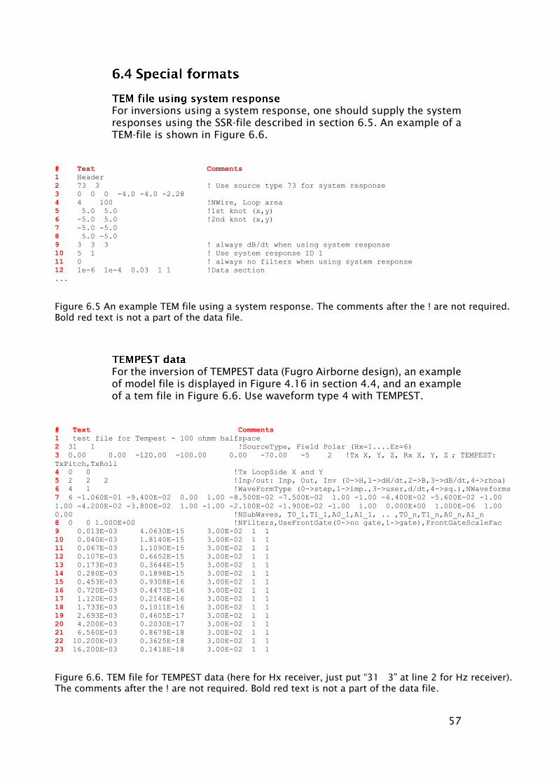
57
For inversions using a system response, one should supply the system
responses using the SSR-file described in section 6.5. An example of a
TEM-file is shown in Figure 6.6.
# Text Comments
1 Header
2 73 3 ! Use source type 73 for system response
3 0 0 0 -4.0 -4.0 -2.28
4 4 100 !NWire, Loop area
5 5.0 5.0 !1st knot (x,y)
6 -5.0 5.0 !2nd knot (x,y)
7 -5.0 -5.0
8 5.0 -5.0
9 3 3 3 ! always dB/dt when using system response
10 5 1 ! Use system response ID 1
11 0 ! always no filters when using system response
12 1e-6 1e-4 0.03 1 1 !Data section
...
Figure 6.5 An example TEM file using a system response. The comments after the ! are not required.
Bold red text is not a part of the data file.
For the inversion of TEMPEST data (Fugro Airborne design), an example
of model file is displayed in Figure 4.16 in section 4.4, and an example
of a tem file in Figure 6.6. Use waveform type 4 with TEMPEST.
# Text Comments
1 test file for Tempest - 100 ohmm halfspace
2 31 1 !SourceType, Field Polar (Hx=1....Ez=6)
3 0.00 0.00 -120.00 -100.00 0.00 -70.00 -5 2 !Tx X, Y, Z, Rx X, Y, Z ; TEMPEST:
TxPitch,TxRoll
4 0 0 !Tx LoopSide X and Y
5 2 2 2 !Inp/out: Inp, Out, Inv (0->H,1->dH/dt,2->B,3->dB/dt,4->rhoa)
6 4 1 !WaveFormType (0->step,1->imp.,3->user,d/dt,4->sq.),NWaveforms
7 6 -1.060E-01 -9.400E-02 0.00 1.00 -8.500E-02 -7.500E-02 1.00 -1.00 -6.400E-02 -5.600E-02 -1.00
1.00 -4.200E-02 -3.800E-02 1.00 -1.00 -2.100E-02 -1.900E-02 -1.00 1.00 0.000E+00 1.000E-06 1.00
0.00 !NSubWaves, T0_1,T1_1,A0_1,A1_1, .. ,T0_n,T1_n,A0_n,A1_n
8 0 0 1.000E+00 !NFilters,UseFrontGate(0->no gate,1->gate),FrontGateScaleFac
9 0.013E-03 4.0630E-15 3.00E-02 1 1
10 0.040E-03 1.8140E-15 3.00E-02 1 1
11 0.067E-03 1.1090E-15 3.00E-02 1 1
12 0.107E-03 0.6652E-15 3.00E-02 1 1
13 0.173E-03 0.3644E-15 3.00E-02 1 1
14 0.280E-03 0.1898E-15 3.00E-02 1 1
15 0.453E-03 0.9308E-16 3.00E-02 1 1
16 0.720E-03 0.4473E-16 3.00E-02 1 1
17 1.120E-03 0.2146E-16 3.00E-02 1 1
18 1.733E-03 0.1011E-16 3.00E-02 1 1
19 2.693E-03 0.4605E-17 3.00E-02 1 1
20 4.200E-03 0.2030E-17 3.00E-02 1 1
21 6.560E-03 0.8679E-18 3.00E-02 1 1
22 10.200E-03 0.3625E-18 3.00E-02 1 1
23 16.200E-03 0.1418E-18 3.00E-02 1 1
Figure 6.6. TEM file for TEMPEST data (here for Hx receiver, just put “31 3” at line 2 for Hz receiver).
The comments after the ! are not required. Bold red text is not a part of the data file.

58
The system response used with waveform type number 5 is supplied in
a separate file called the same name as the mod-file but with the
extension .ssr as seen in Figure 6.7. It has the format:
If 1 ignore the rest of the numbers on the line.
The time between the beginning of one waveform to the beginning of
the next waveform.
The pattern of the waves. There should be integers equal to the first
integer of the line. These numbers are multiplied with the waveform
and one can therefore use waves of differing magnitudes.
The number of reals in line 5 must equal the number of reals in line 4.
Line 3-5 are repeated for the number of system responses in line 2.
The system responses are numbered as they appear in the .ssr file. In
other words with ID’s 1,2,3,…
Remark: The code accepts more than one point at the same time value.
For example times = (0,0,1,1) and responses = (0,1,1,0), which is a
square. However, it might become unstable if the time intervals
become very small (instability has been observed with dt = 1e-16).
# Text Comments
1 Header line
2 1 ! number of system responses in the file
3 2 1600e-6 +1 -1 ! number of waves, period, amplitude pattern
4 0 1e-6 2e-6 3e-6 … ! Times for the system response values
5 0 1 1 0 ! Values for the system response values
Figure 6.7: The SSR input file for the system response. The comments after the ! are not required.
Bold red text is not a part of the file.

59
The DCP data input file contains settings and data for resistivity sound-
ings (section 7.1 – “Header lines in the DCP file”) and resistivity
sounding with induced polarization data (section 7.3 – “Header lines in
DCP file with IP ”).
The DCP-file is a flexible way of storing the measured data. The settings
in the DCP-file are used in the calculation of the forward response in
the AarhusInv code. An example of a DCP data file for a 4-electrode
resistivity sounding is shown in Figure 7.1. The content of the file is
described below.
# Text Comments
1 PACES_01 !Text string
2 22 !SourceType
3 1 1 1 2 !Inp, Out, Inv, OutputMidtPoint
4 -5.0 15.0 -5.0 5.0 100.5 0.05 !XA, XM, XN, XB, data, std
5 -5.0 15.0 -34.0 34.0 99.5 0.05
6 -5.0 15.0 -45.0 45.0 88.9 0.05
7 -5.0 15.0 -45.0 -12.0 102.0 0.05
8 -5.0 15.0 -45.0 -17.0 101.2 0.05
9 -5.0 15.0 -45.0 -19.0 99.7 0.05
Figure 7.1 Data file for electrical data. Source type 22 (4-electrodes on a profile mode), six 4-pole
configurations. The comments after the ! are not required. Bold red text is not a part of the data file.
The header lines of the DCP data file mean the following (line 1-3,
Figure 7.1):
User-defined label describing the DCP-data set. The label is repeated in
the emo-file. Max. 128 characters.
The source type can be one of the following:
Value 20: Schlumberger mode - only the L/2-distance is
specified for the electrode positions.
Value 21: Wenner mode - only the a-distance is specified for the
electrode positions.
Value 22: 4-electrodes on a profile mode. x-positions for the 4
electrodes are specified.
Value 23: 4-electrodes on the earth surface. x and y positions
for the electrodes are specified.
Value 24: 4-electrodes at arbitrary positions on the surface or in
the ground, x, y and z-positions are given for all electrodes.
Value 25: 4-electrodes in a borehole. Only the depth is given for
the electrodes. This source type is used for modelling and
inversion in a 1D cylindrically symmetric coordinate system.

60
The formatting is either:
Value 0 0 0. Input data, output data, and the inversion runs with
electrical potentials.
Value 1 1 1. Input data, output data, and the inversion runs with
apparent resistivity values.
Combinations of the input/output values are not recommended at the
current stage of the program.
The center point of the output is written to the emo-file. Center points
are only written for source type 22 and 23:
Value 1: Center point: (A+B)/2
Value 2: Center point: (M+N)/2
Value 3: Center point: (N+A)/2
Value 4: Center point: (M+B)/2
Each line represents a measured configuration. Electrode positions,
data, and std are specified. A and B are current electrodes. M and N are
potential electrodes. X, Y and Z [m] are electrode positions. For formats
without the z-position, the electrodes are assumed to be on the
surface.
Source type 20: three floats: AM-distance [m], data, std.
Source type 21: three floats: a-distance [m], data, std.
Source type 22 (Figure 7.1): six floats: XA, XM, XN, XB [m], data,
std.
Source type 23: ten floats: XA, YA, XM, YM, XN,YN, XB, YB [m],
data, std.
Source type 24: fourteen floats: XA, YA, ZA, XM, YM, ZM, XN, YN,
ZN, XB, YB, ZB [m], data, std.
Source type 25: six floats: ZA, ZM, ZN, ZB [m], data, std.
The apparent resistivity for source type 20 to 23 is calculated with
respect to a half-space, while 24 and 25 is calculated with respect to a
full-space.
For the inversion of resistivity and IP data, an example of the model file
(mod-file) holding the inversion parameters, prior information,
constraints etc. is shown in Figure 4.6.

61
An example of a dcp-file holding DCIP data is shown below in Figure
7.2 and described in the following. The file is similar to the dcp-file for
resistivity data, but must also be given a waveform and chargeability
data.
# Text Comments
1 DCIP data file !Text
2 272 !SourceType
3 1 1 1 !Inp, Out, Inv
4 1 !#Filters
5 1 1 2.40E+05 !NCutOff, FOrder(1:NCutOff), FCutOff(1:NCutOff)
6 0 !NCutOff, FOrder(1:NCutOff), FCutOff(1:NCutOff)
7 1 !#WaveFormType
8 2 3 3.35 3.50 4 0 1 4 0 -1 4 0 1 !WaveType (2->100%),Npulses, startDCint,endDCind, Ton,Toff,Amp
9 0 !ModelGateTimes
10 -3.75 -1.25 1.25 3.76 1.9805E+01 0.02 1 1 1 !Res: xA,xM,xN,xB,Data,std,ID,FilterID,WaveID
11 -6.26 -1.25 1.25 6.25 2.0381E+01 0.02 2 1 1
12 -8.75 -1.25 1.25 8.75 2.1477E+01 0.02 3 1 1
13 -11.25 -1.25 1.25 11.25 2.2985E+01 0.02 4 1 1
14 -3.75 -1.25 1.25 3.76 4.2789E+02 0.05 1 1 1 2.95E-03 !Char: Pos,Data,std,ID,FilterID,WaveID,Time
15 -3.75 -1.25 1.25 3.76 4.0697E+02 0.05 1 1 1 5.06E-03
16 -3.75 -1.25 1.25 3.76 3.8237E+02 0.05 1 1 1 8.36E-03
17 -3.75 -1.25 1.25 3.76 3.5314E+02 0.05 1 1 1 1.36E-02
18 -3.75 -1.25 1.25 3.76 3.2074E+02 0.05 1 1 1 2.17E-02
19 -3.75 -1.25 1.25 3.76 2.8391E+02 0.05 1 1 1 3.47E-02
20 -3.75 -1.25 1.25 3.76 2.2322E+02 0.05 1 1 1 5.56E-02
21 -6.26 -1.25 1.25 6.25 2.0381E+01 0.05 2 1 1 2.95E-03
22 -6.26 -1.25 1.25 6.25 2.0381E+01 0.05 2 1 1 5.06E-03
…
28 -6.26 -1.25 1.25 6.25 2.0381E+01 0.05 2 1 1 5.56E-02
29 -8.75 -1.25 1.25 8.75 2.1477E+01 0.05 3 1 1 2.95E-03
…
34 -8.75 -1.25 1.25 8.75 2.1477E+01 0.05 3 1 1 3.47E-02
35 -11.25 -1.25 1.25 11.25 2.2985E+01 0.05 4 1 1 2.95E-03
…
45 -11.25 -1.25 1.25 11.25 2.2985E+01 0.05 4 1 1 2.26E-01
Figure 7.2. Data file for DCIP data - source type 272 (four electrodes on a profile). Four different
electrodes configurations have been measured and a low-pass filter is applied. The waveform has a 50%
duty cycle with 4 sec on- and off-time. The comments after the ! are not required. Bold red text and … is
not a part of the data file.
The following description of the DCP-file refers to Figure 7.2.
User-defined label describing the DCP-data set. The label is repeated in
the emo-file. Max. 128 characters.
The source type can be one of the following:
Value 272: Four electrode on a profile model. The x-positions
are specified for the four electrode positions in the data lines.
Value 274: Four electrodes at arbitrary positions on the surface
or in the ground. The x-, y- and z-positions are specified for the
four electrode in the data line.

62
Value: 0 0 0: Input data, output data, and the inversion runs with
electrical potentials.
Value: 1 1 1: Input data, output data, and the inversion runs with
apparent resistivity and chargeability values.
Value = 0: no filters are used and line 5-6 can be left out of the
DCP-file.
Value > 0: number of filters
Two lines per number of filters given in line 4. Fist line holds the low-
pass filters and the second line hold the high-pass filters. Each line hold
the numbers NCutOff, FOrder, FCutOff. FOrder and FCutOff are
repeated NCutOff times.
NCutOff, integer: The number of frequencies defining the filter.
Forder, integer: The order of the Butterworth filter (1 defines a
first order filter, 2 a second order filter).
FCutOff, real: The cut-off frequency for the filters (Hz).
Value >= 1: specifies the number of waveforms.
Value < 1: not allowed
One line per number of waveforms given in line 7. Each line consists of
two integers plus the definition of each pulse (three reals per pulse):
First integer: The transmitter waveform:
o Value 0: Step response.
o Value 1: 50% duty cycle.
o Value 2: 100% duty cycle.
o Value 4: 100% duty cycle, skipping the first pulse.
Second integer: Number of pulses.
Third real: StartDC, the start time of the DC integration.
Fourth real: EndDC, the end time of the DC integration.
For each number of pulses, the four integers/reals described above are
follow by reals for Ton, Toff and Amp:
Ton: The duration of the current on-time.
Toff: The duration of the current off-time. For a 100%
duty cycle, this is 0.
Amp: The amplitude of the pulse. Can be positive and
negative.

63
The modelling of the gate width is not yet implemented
Value 0: no modelling of gate width.
Each data line (line 10-45 in Figure 7.2) is a data point with a resistivity
or a chargeability value. Each data line have nine or ten reals or
integers:
The electrode positions for the measured configuration are listed here.
A and B are current electrodes. M and N are potential electrodes. The
positions needed depends on the source type:
Source type 272: Four reals, xA, xM, xN, xB [m]. For example see
Figure 7.8.
Source type 274: nine reals, xA, yA, zA, xM, yM, zM, xN, yN, zN,
xB, yB, zB [m]. For example see Figure 7.9.
The measured resistivity (res) or chargeability (char) value. If the data
format is 0 (electric potential), the respective units are [V] and [mV/V].
If the data format is 1 (apparent resistivity), the respective units are
[Ohmm] and [mV/V].
The standard deviation on the data.
Each measurement at each electrode configuration is given an ID
number. All the resistivity data are listed fist in the data section with
their individual ID number. Hereafter follow the chargeability data,
which are connected to the resistivity data of the configuration through
their corresponding ID numbers. For example with four different
electrode configurations see Figure 7.9.
The filter used for the measured data. If no filters are used (Nfilters
=0), the filterID must still be set to 1.
The waveform used for the measured data.
Gate center time is only listed for chargeability data lines.
In the data line section, all the resistivity data are listed first, followed
by the IP data. Each data line represents either a measured resistivity
or a chargeability value from one gate on the IP decay.

64
Figure 7.3: Resistivity. Schlumberger configurations with a-spacings
from 1 to 100 m. Source type 21 (Schlumberger mode).
Figure 7.4: Resistivity. Three Wenner configurations with a-spacings of
10 m, 20 m, and 30 m. Source type 20 (Wenner mode).
Figure 7.5: Resistivity. Two 4-pole configurations. XY-layout on the
surface of the earth (source type 23).
Figure 7.6: Resistivity. Four 4-pole configurations in the ground
defined with x, y and z-coordinates for all electrodes (source type 24).
Figure 7.7: Resistivity. Four 4-pole configurations in a borehole.
Electrode positions are defined by their z-coordinate only (source type
25).
# Text Comments
1 Schlumberger config. !text string
2 20 !SourceType
3 1 1 1 1 !Inp, Out, Inv, OutputMidtPoint
4 1.00 99.99 0.05 !AM-spacing, data, std
5 1.33 99.99 0.05
6 1.78 99.97 0.05
7 2.37 99.93 0.05
8 3.16 99.82 0.05
9 4.22 99.59 0.05
10 5.62 99.07 0.05
11 7.50 97.88 0.05
12 10.00 95.30 0.05
13 13.30 90.18 0.05
14 17.80 80.74 0.05
15 23.70 66.31 0.05
16 31.60 48.19 0.05
17 42.20 30.81 0.05
18 56.20 18.88 0.05
19 75.00 13.05 0.05
20 100.00 11.03 0.05
Figure 7.3. Data file for resistivity data - source type 20 (Schlumberger
mode). Three Schlumberger configurations with AM-spacings from 1 to
100 m. The comments after the ! are not required. Bold red text is not a
part of the data file.
# Text Comments
1 3 Wenner config. !text string
2 21 !Source type
3 1 1 1 1 !Inp, Out, Inv, OutputMidtPoint
4 10 47.5 0.05 !AM-spacing, data, std
5 20 99.5 0.05
6 30 88.9 0.05
Figure 7.4. Data file for resistivity data - source type 21 (Wenner mode). 3
Wenner configurations with a-spacing 10 m, 20 m, and 30 m. The
comments after the ! are not required. Bold red text is not a part of the
data file.

65
# Text Comments
1 yx-layout !text string
2 23 !Source type
3 1 1 1 1 !Inp, Out, Inv, OutputMidtPoint
4 0 0 1 5 3 3 9 8 42.2e-3 0.03 !XA,YA,XM,YM,XN,YN,XB,YB,data,std
5 5 5 6 9 8 8 4 3 10.2e-3 0.03
Figure 7.5. Data file for resistivity data - source type 23 (xy-mode). Two 4-
pole configurations. The comments after the ! are not required. Bold red
text is not a part of the data file.
# Text Comments
1 yxz-layout !text string
2 24 !Source type
3 1 1 1 1 !Inp, Out, Inv, OutputMidtPoint
4 0.0 0.0 5.0 0.2 0.0 5.0 0.4 0.0 5.0 0.6 0.0 5.0 9.45 0.01
!XA,YA,ZA,XM,YM,ZM,XN,YN,ZN,XB,YB,ZB,data,std
5 0.0 0.0 5.0 0.2 0.0 5.1 0.4 0.0 5.1 0.6 0.0 5.1 9.63 0.01
6 0.0 0.0 5.0 0.2 0.0 5.2 0.4 0.0 5.2 0.6 0.0 5.2 8.89 0.01
7 0.0 0.0 5.0 0.2 0.0 5.3 0.4 0.0 5.3 0.6 0.0 5.3 7.50 0.01
Figure 7.6. Data file for resistivity data - source type 24 (xyz-mode). Four
4-pole configurations. The comments after the ! are not required. Bold red
text is not a part of the data file.
# Text Comments
1 z-layout !text string
2 25 !Source type
3 1 1 1 1 !Inp, Out, Inv, OutputMidtPoint
4 10.0 10.2 10.4 10.6 10.0 0.01 !ZA,ZM,ZN,ZB,data,std
5 10.0 10.4 10.8 11.2 9.0 0.01
6 10.0 10.6 11.2 11.8 15.0 0.01
7 10.0 11.2 12.4 13.6 16.0 0.01
Figure 7.7. Data file for resistivity data - source type 25 (z-mode,
borehole). Four 4-pole configurations. The comments after the ! are not
required. Bold red text is not a part of the data file.
Figure 7.8 DCIP data from one electrode configuration. Source type 272
- four electrodes on a profile with defined x-coordinate. No filters and
a 100% duty cycle.
Figure 7.9: DCIP data from four different electrode configurations (ID
1-4). Source type 272 – electrode in a layered earth with x-, y- and z-
coordinates. Two different low-pass filters and a 50% duty cycle
waveform.

66
# Text Comments
1 DCIP data !TextLabel
2 272 !SourceType (272->4-electrodes on a profile)
3 1 1 1 !Inp, Out, Inv (0->pot,1->rhoa)
4 0 !#Filters
5 1 !#Waves
6 2 3 3.35 4 4 0 1 4 0 -1 4 0 1 !UserDefWF:
7 0 !ModelG (0 -> No Gates Modeling)
8 0 25 30 55 9.23170E+01 2.00E-02 1 1 1 !Res: xA,xM,xN,B,Res,STD,ID,FilterID,WaveID
9 0 25 30 55 8.38426E+01 5.00E-02 1 1 1 1.1870E-02 !Char: xA,xM,xN,B,Res,STD,ID,FilterID,…
10 0 25 30 55 7.98574E+01 5.00E-02 1 1 1 1.6490E-02 ! …WaveID,time
11 0 25 30 55 7.57249E+01 5.00E-02 1 1 1 2.2800E-02
12 0 25 30 55 7.13599E+01 5.00E-02 1 1 1 3.1610E-02
13 0 25 30 55 6.67997E+01 5.00E-02 1 1 1 4.3840E-02
14 0 25 30 55 6.20620E+01 5.00E-02 1 1 1 6.0810E-02
15 0 25 30 55 5.77763E+01 5.00E-02 1 1 1 8.1020E-02
16 0 25 30 55 5.31190E+01 5.00E-02 1 1 1 1.0980E-01
17 0 25 30 55 4.73344E+01 5.00E-02 1 1 1 1.5880E-01
18 0 25 30 55 4.15553E+01 5.00E-02 1 1 1 2.2810E-01
19 0 25 30 55 3.62228E+01 5.00E-02 1 1 1 3.1770E-01
Figure 7.8. Data file with DCIP data for one electrode configurations, source type 272 (Four electrodes
on a profile). A user defined waveform and no filters. The comments after the ! are not required. Bold
red text is not a part of the data file.
# Text Comments
1 DCIP data !TextLabel
2 274 !SourceType (274->4-electrodes in layered halfspace)
3 1 1 1 !Inp, Out, Inv (0->pot,1->rhoa)
4 2 !NFilters
5 1 1 2.4E+5 !Filter 1, low-pass: NCutOff, FOrder(1:NCutOff), FCutOff(1:NCutOff)
6 0 !Filter 1, high-pass: NCutOff
7 1 1 3.7E+4 !Filter 2, low-pass: NCutOff, FOrder(1:NCutOff), FCutOff(1:NCutOff)
8 0 !Filter 2, high-pass: NCutOff
9 1 !NWaves
10 1 3 3 3.35 4 4 1 4 4 -1 4 4 1 !WaveType, NPulses, startDCint,endDCint, Ton,Toff,Amp
11 0 !ModelG (0 -> No Gates Modeling)
12 -3.75 0 0 -1.25 0 0 1.25 0 0 3.75 0 0 1.9558E+02 2E-02 1 1 1
13 -6.25 0 0 -1.25 0 0 1.25 0 0 6.25 0 0 1.9048E+02 2E-02 2 1 1
14 -8.75 0.2 0 -1.25 0 0 1.25 0 0 8.75 0 0 1.8098E+02 2E-02 3 1 1
15 -11.25 0.5 0 -1.25 0 0 1.25 0 0 11.25 0 0 1.6828E+02 2E-02 4 2 1
16 -3.75 0 0 -1.25 0 0 1.25 0 0 3.75 0 0 8.0432E+01 5E-02 1 1 1 1.0750E-02
17 -3.75 0 0 -1.25 0 0 1.25 0 0 3.75 0 0 7.9386E+01 5E-02 1 1 1 1.3670E-02
18 -3.75 0 0 -1.25 0 0 1.25 0 0 3.75 0 0 7.8243E+01 5E-02 1 1 1 1.7240E-02
19 -3.75 0 0 -1.25 0 0 1.25 0 0 3.75 0 0 7.6955E+01 5E-02 1 1 1 2.1740E-02
…
24 -3.75 0 0 -1.25 0 0 1.25 0 0 3.75 0 0 1.1947E+01 5E-02 1 1 1 2.7890E+00
25 -6.25 0 0 -1.25 0 0 1.25 0 0 6.25 0 0 8.7133E+01 5E-02 2 1 1 2.9530E-03
26 -6.25 0 0 -1.25 0 0 1.25 0 0 6.25 0 0 8.6526E+01 5E-02 2 1 1 3.8740E-03
…
33 -6.25 0 0 -1.25 0 0 1.25 0 0 6.25 0 0 1.2321E+01 5E-02 2 1 1 2.7890E+00
34 -8.75 0.2 0 -1.25 0 0 1.25 0 0 8.75 0 0 9.3111E+01 5E-02 3 1 1 2.9530E-03
35 -8.75 0.2 0 -1.25 0 0 1.25 0 0 8.75 0 0 9.2459E+01 5E-02 3 1 1 3.8740E-03
…
42 -8.75 0.2 0 -1.25 0 0 1.25 0 0 8.75 0 0 9.8374E+00 5E-02 3 1 1 3.5340E+00
43 -11.25 0.5 0 -1.25 0 0 1.25 0 0 11.25 0 0 1.0284E+02 5E-02 4 2 1 2.9530E-03
44 -11.25 0.5 0 -1.25 0 0 1.25 0 0 11.25 0 0 1.0211E+02 5E-02 4 2 1 3.8740E-03
…
51 -11.25 0.5 0 -1.25 0 0 1.25 0 0 11.25 0 0 1.0757E+01 5E-02 4 2 1 3.5340E+00
Figure 7.9. Data file with DCIP data for four electrode configurations, source type 274 (Four electrodes in
a layered half-space). A 50% duty cycle waveform and two different filters. The comments after the ! are
not required. Bold red text and … is not a part of the data file.

67
The SIP data input file contains filter settings and frequency-domain IP
data. An example of the data files is seen in Figure 8.1 and the content
is described below.
# Text Comments
1 SIP data file !Text
2 272 !SourceType
3 1 !#Filters
4 1 1 2.40E+05 !NCutOff, FOrder(1:NCutOff), FCutOff(1:NCutOff)
5 0 !NCutOff, FOrder(1:NCutOff), FCutOff(1:NCutOff)
6 -3.75 -1.25 1.25 3.76 0.04 99.69 0.02 0 1!xA,xM,xN,xB,freq,Data,std,TransID,FilterID
7 -3.75 -1.25 1.25 3.76 0.08 99.60 0.02 0 1
8 -3.75 -1.25 1.25 3.76 0.16 99.50 0.02 0 1
9 -3.75 -1.25 1.25 3.76 0.32 99.40 0.02 0 1
10 -3.75 -1.25 1.25 3.76 0.64 99.31 0.02 0 1
11 -3.75 -1.25 1.25 3.76 1.28 99.23 0.02 0 1
…
19 -3.75 -1.25 1.25 3.76 655 99.01 0.02 0 1
20 -6.26 -1.25 1.25 6.25 0.04 99.53 0.02 0 1
21 -6.26 -1.25 1.25 6.25 0.08 99.47 0.02 0 1
…
35 -6.26 -1.25 1.25 6.25 655 98.68 0.02 0 1
Figure 8.1. Example of SIP file with frequency-domain IP data from measurement at two different
electrode configurations. The source type is 272 – four electrodes on a profile. One low-pass filter is
defined. The comments after the ! are not required. Bold red text and … is not a part of the data file.
User-defined label describing the sip-data set. The label is repeated in
the emo-file. Max. 128 characters.
The source type can be one of the following:
Value 272: Four electrode on a profile model. The x-positions
are specified for the four electrode positions in the data lines.
For 2D inversion, the position of the electrodes must also be listed in
a mesh file, which goes into the inversion. See section 14 – “The mesh
file (2D DCIP)”.
If 0 is indicated, no filters are used and line 4-5 can be left out of the
sip-file.
Two lines per number of filters given in line 4. Fist line holds the low-
pass filters and the second line hold the high-pass filters. Each line
holds the numbers NCutOff, FOrder, FCutOff. FOrder and FCutOff are
repeated NCutOff times.

68
NCutOff, integer: The number of frequencies defining the
filter.
Forder, integer: The order of the Butterworth filter (1
defines a first order filter, 2 a second order filter).
FCutOff, real: The cut-off frequency for the filters (Hz).
If no filters are used, these lines are removed from the sip-file.
Each data line (line 10-45 in Figure 7.2) is a data point with a resistivity
or a chargeability value. Each data line have nine or ten reals or
integers:
The electrode position for the measured configuration is listed here. A
and B are current electrodes. M and N are potential electrodes. The
positions needed depends on the source type:
Source type 272: Four real, xA, xM, xN, xB [m].
The frequency [Hz] at which the data point is measured.
The data value in the data transform determined by the 8th
integer (see
below).
The standard deviation on the data point.
Value 0: Apparent resistivity [Ohmm]
Value 1: Amplitude [Ohm]
Value 2: Phase [-mrad]
Value 3: Real [Ohm]
Value 4: Imaginary [Ohm]
Figure 8.1 shows an example where the data transform is 0-> apparent
resistivity Figure 8.2 shows an example where amplitude and phase
data have been measured for each frequency, so both the data
transform ID 1 and 2 have been used.
The filter used for the measured data. If no filters are used (Nfilters
=0), the filterID must still be set to 1.

69
# Text Comments
1 DCIP data file !Text
2 272 !SourceType
3 1 !#Filters
4 1 1 2.40E+05 !NCutOff, FOrder(1:NCutOff), FCutOff(1:NCutOff)
5 0 !NCutOff, FOrder(1:NCutOff), FCutOff(1:NCutOff)
6 -3.75 -1.25 1.25 3.76 0.04 1.058 0.10 1 1 !xA,xM,xN,xB,freq,…
7 -3.75 -1.25 1.25 3.76 0.04 1.81 0.10 2 1 ! …Data,std,TransID,FilterID
8 -3.75 -1.25 1.25 3.76 0.08 1.057 0.10 1 1
9 -3.75 -1.25 1.25 3.76 0.08 2.01 0.10 2 1
10 -3.75 -1.25 1.25 3.76 0.16 1.056 0.10 1 1
11 -3.75 -1.25 1.25 3.76 1.16 1.08 0.10 2 1
…
19 -3.75 -1.25 1.25 3.76 655 0.11 0.10 2 1
20 -6.26 -1.25 1.25 6.25 0.04 1.045 0.10 1 1
21 -6.26 -1.25 1.25 6.25 0.04 1.75 0.10 2 1
…
35 -6.26 -1.25 1.25 6.25 655 1.06 0.10 2 1
Figure 8.2. Example of a SIP data file with data measured as amplitude and phase (data
transform 1 and 2). The comments after the ! are not required. Bold red text and … is not a
part of the data file.

70
The HEM data input file is specialized to input helicopter EM data or
ground conductivity meter data like DualEM or EM31/EM38 data. The
settings in the HEM-file are used in the calculation of the forward
response in the AarhusInv code. Sources are limited to dipoles. An
example of a HEM data file is shown in Figure 9.1.
# Text Comments
1 HEM data - BGR bird !Textstring
2 0.00 0.00 -40.00 8.00 0.00 -40.00 !Tx X, Y, Z, Rx X, Y, Z
3 3.750E+02 8.270E+01 5.0E-02 7.920E+00 5 1 3 !Freq,DataVal,DataValStd,CoilSep, ....
4 3.750E+02 1.293E+02 5.0E-02 7.920E+00 6 1 3 !..DataType,SourceType(1),Receiverype(1-3)
5 1.778E+03 2.724E+02 2.5E-02 7.910E+00 5 1 3
6 1.778E+03 2.393E+02 2.5E-02 7.910E+00 6 1 3
7 8.510E+03 5.803E+02 5.0E-02 7.960E+00 5 1 3
8 8.510E+03 2.869E+02 5.0E-02 7.960E+00 6 1 3
9 3.783E+04 8.673E+02 2.5E-02 8.030E+00 5 1 3
10 3.783E+04 2.839E+02 2.5E-02 8.030E+00 6 1 3
11 1.285E+05 1.064E+03 5.0E-02 7.920E+00 5 1 3
12 1.285E+05 3.125E+02 5.0E-02 7.920E+00 6 1 3
Figure 9.1. Data file for frequency domain HEM data. The transmitter is a vertical magnetic dipole.
One imaginary and one real part are stored for the frequencies. The data shown is for a two layer
model with resisitivites 100ohm-m/10 ohm-m and thickness of the first layer of 10 m. The
comments after the ! are not required. Bold red text is not a part of the data file.
User-defined label describing the HEM data set. The label is repeated
in the emo-file. Max. 128 characters.
The x, y and z-coordinates of the transmitter (first three numbers) and
the receiver (last three numbers). The z-coordinates must be negative
or zero (the receiver or the transmitter must be in the air or on the
ground).
Each line is one data point (one frequency, real ppm, imaginary ppm,
amplitude or phase). The line consists of seven numbers:
Real. Transmitter frequency in Hz (1/s).
Real. The data value with the unit indicated in column 5.
Real. The relative standard deviation on the data value.
Real. The coil-separation in meters. In the code it is always
assumed that the transmitter has coordinates (0,0,Transmitter

71
z) and the receiver has coordinates (Coil-Separation, 0, Receiver
z), thus overriding information given on line 2.
Integer. The type of data:
Value 0: Apparent resistivity
Value 2: Phase
Value 5: Real in ppm**
Value 6: Imaginary in ppm**
Integer. The source type - source direction. 1 - Hx, 2 - Hy and 3
- Hz.
Integer. The receiver type. 1 - Hx, 2 - Hy and 3 - Hz.
**For data in ppm which are normalized by the primary field the Hx (or
Hr) is normalized by the primary Hz since the primary Hr (in a
homogeneous space) is zero for transmitter and receiver loops at the
same altitude

72
The FEM data input file is somewhat similar to the tem input file (“The
TEM file (time domain data)” on page 48). The fem input file contains
transmitter geometry and low- and high-pass of the receiver and the
data.
The fem-file is a flexible way of storing the measured data. The settings
in the fem-file are used in the calculation of the forward response in
the AarhusInv code. An example of a FEM data file for an offset loop
configuration sounding is shown in Figure 10.1.
# Text Comments
1 Created by Emma
2 0.0 0.0 0.0 100.0 0.0 0.0 !Tx X, Y, Z, Rx X, Y, Z
3 40.0 40.0 !Loop dimensions
4 2 2 !Inp/out: Inp, Out (0->H,2->B,4->rhoa)
5 3 !NFilters (0->no filters at all, else 1,2 ...)
6 1 1 2.40E+05 !LP/HP: NCutOff (0->no filter),FOrder(1,NCutOff),FCutOff(1,NCutOff)(Hz)
7 0 !LP/HP: NCutOff (0->no filter),FOrder(1,NCutOff),FCutOff(1,NCutOff)(Hz)
8 1 1 2.40E+05 !LP/HP: NCutOff (0->no filter),FOrder(1,NCutOff),FCutOff(1,NCutOff)(Hz)
9 0 !LP/HP: NCutOff (0->no filter),FOrder(1,NCutOff),FCutOff(1,NCutOff)(Hz)
10 1 1 3.70E+04 !LP/HP: NCutOff (0->no filter),FOrder(1,NCutOff),FCutOff(1,NCutOff)(Hz)
11 0 !LP/HP: NCutOff (0->no filter),FOrder(1,NCutOff),FCutOff(1,NCutOff)(Hz)
12 2.371E-01 5.506E-18 5.00E-02 3 0 7 1
13 2.371E-01 1.563E-15 5.00E-02 4 0 7 1
14 3.162E-01 9.233E-18 5.00E-02 3 0 7 1
15 3.162E-01 2.084E-15 5.00E-02 4 0 7 1
16 4.217E-01 1.549E-17 5.00E-02 3 0 7 1
17 4.217E-01 2.778E-15 5.00E-02 4 0 7 1
18 5.623E-01 2.586E-17 5.00E-02 3 0 7 1
19 5.623E-01 3.703E-15 5.00E-02 4 0 7 1
20 7.499E-01 4.312E-17 5.00E-02 3 0 7 1
21 7.499E-01 4.934E-15 5.00E-02 4 0 7 1
22 1.000E+00 7.159E-17 5.00E-02 3 0 7 1
23 1.000E+00 6.573E-15 5.00E-02 4 0 7 1
24 . . . . . . .
25 . . . . . . .
26 1.000E+05 2.827E-12 5.00E-02 3 0 7 1
27 1.000E+05 -2.648E-12 5.00E-02 4 0 7 1
28 1.334E+05 2.437E-12 5.00E-02 3 0 7 1
29 1.334E+05 -2.334E-12 5.00E-02 4 0 7 1
30 1.778E+05 2.112E-12 5.00E-02 3 0 7 1
31 1.778E+05 -2.055E-12 5.00E-02 4 0 7 1
32 2.371E+05 1.848E-12 5.00E-02 3 0 7 1
33 2.371E+05 -1.815E-12 5.00E-02 4 0 7 1
34 3.162E+05 1.645E-12 5.00E-02 3 0 7 1
35 3.162E+05 -1.626E-12 5.00E-02 4 0 7 1
36 4.217E+05 1.505E-12 5.00E-02 3 0 7 1
37 4.217E+05 -1.506E-12 5.00E-02 4 0 7 1
38 5.623E+05 1.427E-12 5.00E-02 3 0 7 1
39 5.623E+05 -1.491E-12 5.00E-02 4 0 7 1
40 7.499E+05 1.419E-12 5.00E-02 3 0 7 1
41 7.499E+05 -1.672E-12 5.00E-02 4 0 7 1
42 1.000E+06 1.177E-12 5.00E-02 3 0 7 1
43 1.000E+06 -2.310E-12 5.00E-02 4 0 7 1
Figure 10.1. Data file for frequency domain data. The transmitter is a 40 x 40 m square loop and the
receiver is offset 100 m. One imaginary and one real part are stored for the frequencies. The
comments after the ! are not required. Bold red text is not a part of the data file.

73
User-defined label describing the FEM data set. The label is repeated in
the emo-file. Max. 128 characters.
The x, y and z-coordinates of the transmitter (first three numbers) and
the receiver (last three numbers).
Side-lengths of the transmitter loop.
The input and the output format of the FEM data. First integer is input,
second integer is output:
Value 0: Magnetic field intensity (H)
Value 2: Magnetic induction (B)
Value 4: Apparent resistivity
Number of filters. If 0 is indicated, no filters are used.
Two lines per number of filters as given in line 5. First line holds the
low-pass filters, second line holds the high-pass filters. High-pass
filters are most often not present. The format of one line is [NCutOff,
FOrder, FCutOff(1:NCutOff)]
NCutOff (integer) is an integer with the number of frequencies
defining the filter.
FOrder (integer) is the order of the filter (1 defines a first order
filter, 2 a second order filter).
FCutOff (real) is the cut-off frequency for the filters.
FOrder and FCutOff are repeated NCutOff times.
Each line is one data point (one frequency, real or imaginary part or
amplitude and phase). The line consists of seven numbers:
Real. Transmitter frequency.
Real. The data value with the unit indicated in line 4.
Real. The relative standard deviation on the data value.
Integer. The type of data: 0 - apparent resistivity, 1 - amplitude,
2 - phase, 3 - real or 4 - imaginary part.
Integer. The filter number given in line 5 (0 for dummy).

74
Integer. The source type. 1- horizontal magnetic x-directed
dipole, 2- horizontal magnetic y-directed dipole, 3 vertical
magnetic dipole, 7 - rectangular loop, 72 – segmented loop, 12
- circular central loop and 13 - circular offset loop. For further
specification see section: 6.1- Header lines in the TEM file.
Integer. The receiver type. 1 - Hx, 2 – Hy, 3 – Hz, 4 – Ex, 5 - Ey
and 6 – Ez.

75
The MRS data input file contains transmitter/receiver loop geometry,
Earth’s magnetic field information and data obtained from magnetic
resonance soundings. An example of a MRS data file for a separated-
loop configuration sounding is shown in Figure 13.1).
# Text Comments
1 MRS data file
2 72 1 !Source type (Tx/Rx), Loop configuration (0-> coindident, 1-> separate)
3 0.0 0.0 0.0 0.0 0.0 0.0 !X,Y,Z coordinates of Tx [and Rx] loop centers
4 4 !Number of Tx loop apexes (loop is centralized at origin)
5 -50 -50 !x1,y1 -> coordinates of the 1st apex
6 50 -50 !x2,y2 -> coordinates of the 2nd apex
7 50 50 !x3,y3 -> coordinates of the 3rd apex
8 -50 50 !x4,y4 -> coordinates of the 4th apex
9 4 !Number of Rx loop apexes (loop is centralized at origin)
10 -25 -25 !x1,y1 -> coordinates of the 1st apex
11 25 -25 !x2,y2 -> coordinates of the 2nd apex
12 25 25 !x3,y3 -> coordinates of the 3rd apex
13 -25 25 !x4,y4 -> coordinates of the 4th apex
14 70 2 !Earth’s magnetic field inclination and declination (degree)
15 0.04 !Tx pulse length (s)
16 1 1 !Number of wire turns on Tx and Rx loops
17 2132.8 !Larmor frequency (Hz)
18 282 !Ground temperature (K)
19 0.0668 1.16E-007 9.00E-002 1.11E-001 0 0 !time(s), data(V), STD, q(As), freq. offset, ID
20 0.1164 9.90E-008 9.32E-002 1.39E+001 0 0
21 0.1660 6.76E-008 1.24E-001 1.11E-001 0 0
22 0.2160 5.20E-008 1.42E-001 1.11E-001 0 0
23 0.2650 3.87E-008 1.47E-001 1.11E-001 0 0
24 0.3150 3.47E-008 1.74E-001 1.11E-001 0 0
25 0.3640 2.52E-008 3.09E-001 1.11E-001 0 0
25 0.4140 2.10E-008 4.22E-001 1.11E-001 0 0
27 0.4640 1.73E-008 5.59E-001 1.11E-001 0 0
28 0.5130 1.42E-008 5.32E-001 1.11E-001 0 0
29 0.0668 1.60E-007 9.79E-002 1.59E-001 0 0
30 0.1164 1.16E-007 9.81E-002 1.59E-001 0 0
31 . . . . . . .
32 . . . . . . .
33 0.5130 2.23E-008 3.29E-001 1.59E-001 0 0
34 . . . . . . .
35 . . . . . . .
36 0.0668 1.32E-007 1.15E-001 1.39E+001 0 0
37 0.1164 9.90E-008 9.32E-002 1.39E+001 0 0
38 0.1660 7.56E-008 1.05E-001 1.39E+001 0 0
39 0.2160 6.34E-008 8.19E-002 1.39E+001 0 0
40 0.2650 5.46E-008 1.80E-001 1.39E+001 0 0
41 0.3150 4.58E-008 1.71E-001 1.39E+001 0 0
42 0.3640 3.97E-008 1.90E-001 1.39E+001 0 0
43 0.4140 3.38E-008 1.95E-001 1.39E+001 0 0
44 0.4640 2.41E-008 2.53E-001 1.39E+001 0 0
45 0.5130 2.07E-008 3.47E-001 1.39E+001 0 0
Figure 10.11.1. The MRS data file. A separated-loop configuration (Tx: 100-m side, Rx: 50-m side) is
used. The comments after the ! are not required. Bold red text is not a part of the data file.
User-defined label describing the MRS-data set. The label is repeated
in the emo-file. Max. 128 characters.

76
The MRS forward modeling code supports the following source type:
Value 72. Segmented loop source. This type is used for
arbitrarily shaped loops. The segmented loop source is also
described in section 6.2- “Header lines with segmented loop
and front gate”.
Value 0: coincident loop configuration
Value 1: separated loop configuration
Transmitter and receiver loop center coordinates. In the case of
coincident loop configuration, only three reals appear in this line.
This integer gives the number of transmitter wire segments used to
define the segmented loop.
X- and y-coordinates of Tx wire end-point (loop is centralized at origin).
The loop is automatically closed by connecting the last point to the
first point.
This integer gives the number of receiver wire segments used to define
the segmented loop.
X- and y-coordinates of Tx wire end-point (loop is centralized at origin).
The loop is automatically closed by connecting the last point to the
first point.
Inclination of the Earth’s magnetic field, in degrees.
Declination of the Earth’s magnetic field in the loop coordinate system,
in degrees.
Transmitter pulse length, in sec. This information is used is frequency-
offset is taken into account (see data section below).
If coincident-loop configuration is used (0 value in line 2, integer 2),
one real value appears here.
Resonance (Larmor) frequency calculated from the Earth’s field
intensity.
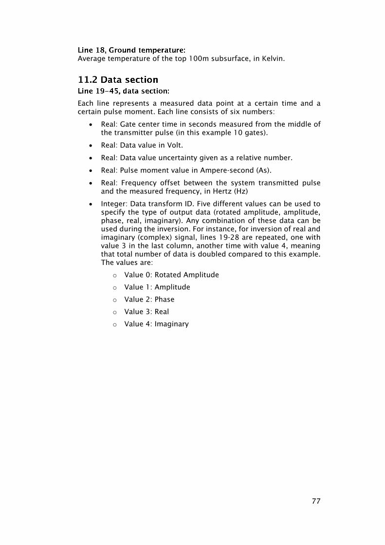
77
Average temperature of the top 100m subsurface, in Kelvin.
Each line represents a measured data point at a certain time and a
certain pulse moment. Each line consists of six numbers:
Real: Gate center time in seconds measured from the middle of
the transmitter pulse (in this example 10 gates).
Real: Data value in Volt.
Real: Data value uncertainty given as a relative number.
Real: Pulse moment value in Ampere-second (As).
Real: Frequency offset between the system transmitted pulse
and the measured frequency, in Hertz (Hz)
Integer: Data transform ID. Five different values can be used to
specify the type of output data (rotated amplitude, amplitude,
phase, real, imaginary). Any combination of these data can be
used during the inversion. For instance, for inversion of real and
imaginary (complex) signal, lines 19-28 are repeated, one with
value 3 in the last column, another time with value 4, meaning
that total number of data is doubled compared to this example.
The values are:
o Value 0: Rotated Amplitude
o Value 1: Amplitude
o Value 2: Phase
o Value 3: Real
o Value 4: Imaginary

78
The MT data input file contains settings and data for MT soundings.
The following refers to the data file in Figure 12.1.
User-defined label describing the MTD-data set. The label is repeated
in the emo-file. Max. 128 characters.
The polarization can be one of the following:
Value 1: Ex/Hy.
Value 2: Ey/Hx.
Each line represents a measured data point at a certain frequency.
First real: Frequency in Hz.
Second real: Data value
Third real: Data value uncertainty given as a relative number, i.e.
0.05 for 5%.
Fourth integer: Data type. 0 is apparent resistivity; 2 is phase.
Figure 12.1: A simple MT data file with synthetic RMT data calculated
at a variety of frequencies. Each frequency has two data values - an
apparent resistivity value and a phase value.
# comment
1 Test-file, MTD
2 1
3 1.000E+04 4.284E+01 5.00E-02 0
4 1.000E+04 2.904E+01 2.50E-02 2
5 1.500E+04 3.653E+01 5.00E-02 0
6 1.500E+04 3.276E+01 2.50E-02 2
7 2.000E+04 3.353E+01 5.00E-02 0
8 2.000E+04 3.630E+01 2.50E-02 2
9 3.000E+04 3.150E+01 5.00E-02 0
10 3.000E+04 4.134E+01 2.50E-02 2
11 : : : :
12 9.000E+05 6.742E+01 5.00E-02 0
13 9.000E+05 5.577E+01 2.50E-02 2
14 1.000E+06 6.956E+01 5.00E-02 0
15 1.000E+06 5.576E+01 2.50E-02 2
Figure 12.1. Data file for MT data. The comments after the ! are not
required. Bold red text is not a part of the data file.

79
The SWD data input file contains settings and data for seismic surface
wave dispersion curves obtained from surface wave soundings. The
following refers to the data file in Figure 13.1.
User-defined label describing the SWD-data set. The label is repeated
in the emo-file. Max. 128 characters.
The data can be either wavenumber (0) or phase velocity (1). The
integers specifies for the format of:
First integer: Input.
Second integer: Inversion.
Third integer: Output.
Thus, data can be given as wavenumber on input, an inversion
parameter, but with the output in phase velocity.
Each line represents a point on the dispersion curve obtained from an
SWD analysis.
First real: Frequency in Hz.
Second real: Data value (phase velocity or wavenumber)
Third real: Data value uncertainty given as a relative number, i.e.
0.05 for 5%.
Fourth integer: mode of the dispersion curve. 1 - fundamental
mode, 2 - first ?.
Figure 13.1: A simple dispersion curve from a SWD field data set at a
variety of frequencies and two different modes.
# comment
1 Test dataset for SWD
2 1 1 1 !Inp, Out, Inv (0->wavenumber,1->phase vel.)
3 12.000 596.640 0.05 1
4 13.000 493.091 0.05 1
5 14.000 400.204 0.05 1
6 15.000 345.577 0.05 1
7 16.000 341.144 0.05 1
8 17.000 310.823 0.05 1
9 18.000 305.197 0.05 1
10 19.000 298.301 0.05 1
11 20.000 288.143 0.05 1
12 21.000 287.562 0.05 1
13 22.000 285.207 0.05 1

80
14 23.000 282.323 0.05 1
15 24.000 273.119 0.05 1
16 25.000 261.654 0.05 1
17 26.000 263.770 0.05 1
19 21.000 287.562 0.05 2
20 22.000 285.207 0.05 2
21 23.000 282.323 0.05 2
22 24.000 273.119 0.05 2
23 25.000 261.654 0.05 2
24 26.000 263.770 0.05 2
Figure 13.1. Data file for SWD data. The comments after the ! are not
required. Bold red text is not a part of the data file.

81
The mesh file (msh-file) is only in use for 2D inversion of DC data and
only in that case has to be specified (The 2D option is set in the model
file as described in “The model file” on page 13).
The msh-file is used to define a finite difference mesh for 2D modelling
and inversions. In the file, the x-z plane is divided into a structured
grid. Note that electrodes must be placed on nodes.
An example of a mesh files is shown in Figure 14.1.
The following description follows the example in Figure 14.1.
Number of nodes in the x- and z-direction
The UTMx coordinates of the nodes.
The UTMy coordinates of the nodes.
X-positions along the profile. 0 is usually the position of the first
electrode.
Y-positions along the profile.
Comments
1 547 47 !NxNodes, NzNodes
2
3 4.9445381589E+05 4.94687722572E+05 … 4.9568396256E+05 !UTMx (size NxNodes)
4 6.1779395006E+06 6.17764146596E+06 … 6.1765714950E+06 !UTMy (size NxNodes)
5
6 -6.287501+02 -2.501939E+0.2 … 1.215919E+03 !x position (size NxNodes)
7 0 0 … 0 !y position (size NxNodes)
8
9 3.9570E+01 3.9570E+01 … 4.2600E+01 !z elevation, shallowest…
10 3.9070E+01 3.9070E+01 … 3.9770E+01 … node (sixe NxNodes)
11 3.8054E+01 3.8560E+01 … 3.9110E+01
…
55 -1.7381E+03 -1.7381E+03 … -1.7381E+03 !z elevation, deepest node
56
57 119 !Number of electrode
58 1 38 1 !El. Nr, Xnode nr, Znode nr
59 2 42 1
60 3 46 1
…
176 119 510 1
Figure 14.1. meh-file. The comments after the ! are not required. Bold red text is not a
part of the data file.

82
One line for each node in the z-direction (NzNodes). The first line must
be the shallowest node. Each line has the length NxNodes.
The number of electrodes used in the profile
One line for each electrode. Each electrode is assigned an Xnode and
Znode number, which is linked to its position through the node
numbers. Note: Electrodes must be placed on a node.
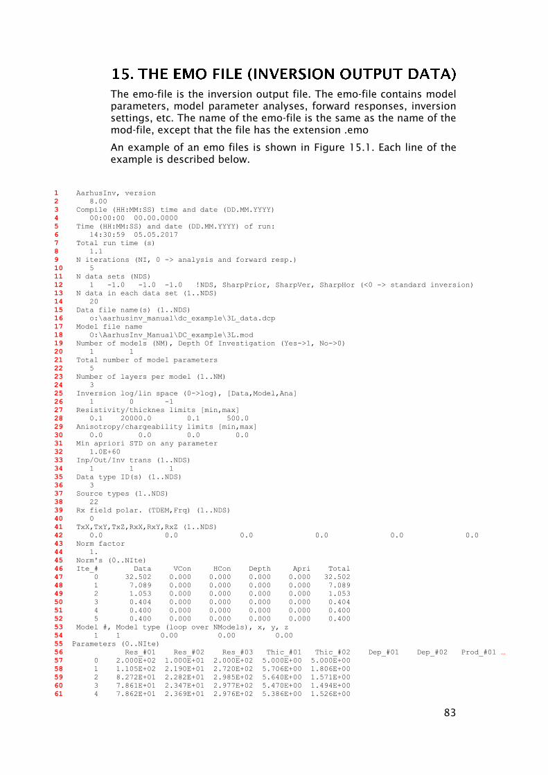
83
The emo-file is the inversion output file. The emo-file contains model
parameters, model parameter analyses, forward responses, inversion
settings, etc. The name of the emo-file is the same as the name of the
mod-file, except that the file has the extension .emo
An example of an emo files is shown in Figure 15.1. Each line of the
example is described below.
1 AarhusInv, version
2 8.00
3 Compile (HH:MM:SS) time and date (DD.MM.YYYY)
4 00:00:00 00.00.0000
5 Time (HH:MM:SS) and date (DD.MM.YYYY) of run:
6 14:30:59 05.05.2017
7 Total run time (s)
8 1.1
9 N iterations (NI, 0 -> analysis and forward resp.)
10 5
11 N data sets (NDS)
12 1 -1.0 -1.0 -1.0 !NDS, SharpPrior, SharpVer, SharpHor (<0 -> standard inversion)
13 N data in each data set (1..NDS)
14 20
15 Data file name(s) (1..NDS)
16 o:\aarhusinv_manual\dc_example\3L_data.dcp
17 Model file name
18 O:\AarhusInv_Manual\DC_example\3L.mod
19 Number of models (NM), Depth Of Investigation (Yes->1, No->0)
20 1 1
21 Total number of model parameters
22 5
23 Number of layers per model (1..NM)
24 3
25 Inversion log/lin space (0->log), [Data,Model,Ana]
26 1 0 -1
27 Resistivity/thicknes limits [min,max]
28 0.1 20000.0 0.1 500.0
29 Anisotropy/chargeability limits [min,max]
30 0.0 0.0 0.0 0.0
31 Min apriori STD on any parameter
32 1.0E+60
33 Inp/Out/Inv trans (1..NDS)
34 1 1 1
35 Data type ID(s) (1..NDS)
36 3
37 Source types (1..NDS)
38 22
39 Rx field polar. (TDEM,Frq) (1..NDS)
40 0
41 TxX,TxY,TxZ,RxX,RxY,RxZ (1..NDS)
42 0.0 0.0 0.0 0.0 0.0 0.0
43 Norm factor
44 1.
45 Norm's (0..NIte)
46 Ite_# Data VCon HCon Depth Apri Total
47 0 32.502 0.000 0.000 0.000 0.000 32.502
48 1 7.089 0.000 0.000 0.000 0.000 7.089
49 2 1.053 0.000 0.000 0.000 0.000 1.053
50 3 0.404 0.000 0.000 0.000 0.000 0.404
51 4 0.400 0.000 0.000 0.000 0.000 0.400
52 5 0.400 0.000 0.000 0.000 0.000 0.400
53 Model #, Model type (loop over NModels), x, y, z
54 1 1 0.00 0.00 0.00
55 Parameters (0..NIte)
56 Res_#01 Res_#02 Res_#03 Thic_#01 Thic_#02 Dep_#01 Dep_#02 Prod_#01 …
57 0 2.000E+02 1.000E+01 2.000E+02 5.000E+00 5.000E+00
58 1 1.105E+02 2.190E+01 2.720E+02 5.706E+00 1.806E+00
59 2 8.272E+01 2.282E+01 2.985E+02 5.640E+00 1.571E+00
60 3 7.861E+01 2.347E+01 2.977E+02 5.470E+00 1.494E+00
61 4 7.862E+01 2.369E+01 2.976E+02 5.386E+00 1.526E+00

84
62 5 7.865E+01 2.371E+01 2.976E+02 5.373E+00 1.531E+00
63 Analysis: apriori/coupled/uncoupled, (-1 -> unconstrained)
64 -1.00E+00 -1.00E+00 -1.00E+00 -1.00E+00 -1.00E+00 -1.00E+00 -1.00E+00
65 2.52E-02 -1.00E+00 2.50E-02 1.33E+00 -1.00E+00 1.33E+00 1.88E+00 1.30E+00
66 1.00E+03 1.00E+03 1.00E+03 1.00E+03 1.00E+03 1.00E+03 1.00E+03 1.00E+03
67 Apriori parameters
68 200.0 10.0 200.0 5.0 5.0 5.0 10.0
69 Constraints: CouplingWidth/Vertical/Horizontal (-1 -> no constraint, 1:CouplingWidth-1)
70 0
71 None normalized, normalized covariance matrix (0->not present, 1->present)
72 0 0
73 Output, data set #, model # for dataset
74 1 1
75 Data type ID
76 3
77 Ax Mx Nx Bx Inp_Data STD DSet# Ite#005 …
78 -3.8000E+00 -1.2000E+00 1.2000E+00 3.8000E+00 7.948E+01 2.00E-02 1 7.80743E+01 …
79 -6.2000E+00 -1.2000E+00 1.2000E+00 6.2000E+00 7.573E+01 2.00E-02 1 7.74376E+01 …
80 -8.8000E+00 -1.2000E+00 1.2000E+00 8.8000E+00 7.817E+01 2.00E-02 1 7.86972E+01 …
… … … … … … … … …
96 -1.9500E+02 -3.2500E+01 3.2500E+01 1.9500E+02 2.724E+02 2.00E-02 1 2.71551E+02 …
97 -2.5000E+02 -3.2500E+01 3.2500E+01 2.5000E+02 2.815E+02 2.00E-02 1 2.80172E+02 …
98 Depth Of Investigation (DOI)
99 DOI # of Depths
100 19
101 Depth1, DepthN
102 2.500 300.000
103 Abs_High Abs_Low
104 1.500 0.750
105 Rel_High Rel_Low
106 0.050 0.020
107 Model #
108 1
109 Depths Sensitivity Cummulated Normalized
110 2.500E+00 8.206E+00 1.943E+01 1.000E+00
111 7.803E+00 3.148E+00 1.122E+01 5.777E-01
112 1.375E+01 1.833E+00 8.077E+00 4.157E-01
113 2.042E+01 1.260E+00 6.245E+00 3.214E-01
114 2.790E+01 9.520E-01 4.984E+00 2.565E-01
115 3.628E+01 7.628E-01 4.032E+00 2.075E-01
116 4.568E+01 6.300E-01 3.270E+00 1.683E-01
117 5.622E+01 5.266E-01 2.640E+00 1.358E-01
118 6.804E+01 4.401E-01 2.113E+00 1.087E-01
119 8.130E+01 3.650E-01 1.673E+00 8.610E-02
120 9.616E+01 2.990E-01 1.308E+00 6.731E-02
121 1.128E+02 2.411E-01 1.009E+00 5.192E-02
122 1.315E+02 1.910E-01 7.678E-01 3.952E-02
123 1.525E+02 1.486E-01 5.768E-01 2.969E-02
124 1.760E+02 1.137E-01 4.282E-01 2.204E-02
125 2.023E+02 8.559E-02 3.145E-01 1.619E-02
126 2.319E+02 6.354E-02 2.289E-01 1.178E-02
127 2.650E+02 4.661E-02 1.654E-01 8.512E-03
128 3.000E+02 1.188E-01 1.188E-01 6.113E-03
129 DOI absolute [Abs_High Abs_Low]
130 88.339 133.472
131 DOI relative [Rel_High Rel_Low]
132 115.723 185.147
Figure 15.1. emo file for a simple inversion of one DC dataset with one model and no constrain or
prior information. Bold red text is not a part of the data file
Lines 1-42 contain information about which data and model files have
been used. This information comes from the data files, the emo-file,
and the con-file. A few comments on specific lines:

85
Lines 21-22: For a DC inversion, a model with three layers gives
three resistivity values and two thickness. A total of five
parameters.
Lines 25-32: These settings are set in the con-file. Anisotropy is
not implemented in the inversion-code yet. Therefore, the
numbers in line 30 will always be 0 0 0 0.
Lines 35-36: Each data type is associated with an ID-number in
the inversion code.
Line 43-70 contain information on the inversion result with respect to
models and data. A few specific comments follow.
Lines 43-44: Norm factor. Norms are scaled by the factor norm-
factor.
Lines 45-52: The norm (residual) progress through the iteration
steps. Column 1: Iteration number. Column 2-6: residuals for
data, vertical constraints, horizontal constraints (resistivities
and depths only), horizontal depth constraints, model prior.
Column 7: Total residual.
Lines 53-54: Model number
Lines 57-62: The model parameters through the iteration steps.
No values for depths or the product of resistivities and thickness
are given. Start model is iteration number 0 (line 57). Model
parameters for the last iteration (line 62) are the final inversion
result.
Line 64: Parameter analysis on prior values from the parameters
in line 62. -1 is an unconstrained parameter.
Line 65: Coupled model parameters analysis (with respect to the
parameters in line 62) where the information from the
constraints are taken into account. -1 is for an undetermined
parameter.
Line 66: Uncoupled model parameter analysis (with respect to
the parameters in line 62). No constraint information.
In the model parameter analysis, the standard deviation on the
parameter p, STDp, as given in the emo-file, is calculated as:
1),cov(expSTD ppp
where cov(p,p) is the covariance of the p’th parameter in the covariance
matrix.
Lines 67-68: Prior model parameters (starting model).
Line 70: Constraints mode as given in the mod-file

86
Line 71-72: In the con-file, AarhusInv can be customized to write
out the covariance matrix and the normalized covariance matrix.
Line 73-76 contains the settings from the mod-files.
Lines 78-97: Data belonging to the dataset (20 electrode
configurations). Column 1-4: Position of electrodes. Column 5:
Input data. Column 6: data STD. Column 7: Dataset number.
Column 8-end: Forward data for each iterations step.
The last section of the emo-files (line 98-end) describes the data used
for calculating the depth of investigation (DOI) for the final model.
Information on the DOI is crucial for interpreting the geophysical
models, as the validity of the models varies considerably with data
noise and parameter distribution.
The calculated DOI is based on an approximated covariance analysis
that uses both the actual model output from the inversion and the
actual number of data and theirdata standard deviation.
Line 100: Number of layers as defined in the con-file. Default
value is 19 layers.
Line 101-102: Depth1 is the thickness of the first layer (default
2.5 m) and DepthN is the depth to the last layer boundary
(default 300 m). The values are defined in the con-file.
Line 103-104: High and low (shallow and deep) absolute values
for DOI calculations. These values determine for which absolute
sensitivity values, the absolute DOI values are given (line 130).
The values are defined in the con-file.
Line 105-106: High and low (shallow and deep) relative values
for DOI calculations. These values determine for which relative
sensitivities value (e.g. 0.05 (5%) of total sensitivity), the relative
DOI values are given (line 132). The values are defined in the
con-file.
Column 1: Depth of the DOI model.
Column 2: Sensitivity at the given depth.
Column 3: Cumulated sensitivity (cumulated from the bottom).
Column 4: Normalized cumulated sensitivity.
Note: If the inversion had more parameters, these columns would be
repeated for each parameter (except thickness and depth).

87
Line 130: DOI absolute - the depths where cumulated sensitivity
(listed in line 104) is reached.
Line 132. DOI relative - the depths where normalized cumulated
sensitivity (listed in line 106) is reached.
For inversion of 2D DC, 2D HEM, 1D/2D DCIP and 1D MRS, the DOI data
format varies from the example above. Instead of the absolute analysis,
a cumulated approximate analysis (CAA) is given.
An example from an 2D inversion of resistivity and temperature data
is given in Figure 15.2. The lines different from the previous example
are commented below.
Column 2: Normalized cumulated sensitivity for the resistivity
model.
Column 3: CCA for the resistivity model.
Column 4: Normalized cumulated sensitivity for the temperature
model.
Column 5: CCA for the temperature model.
Column 6-8: The square root of the Jacobian (without
normalization). These columns show the parameter
correlations.
128 Depth Of Invistigation (DOI)
129 DOI # of Depths
130 24
131 Depth1, DepthN
132 1.320 186.466
133 CAA_High CAA_Low
134 2.000 5.000
135 Rel_High Rel_Low
136 0.050 0.020
137 Model #
138 1
139 Depths Res# Relative CAA Temp# Relative CAA CumGTG:[Res#Res#] [Res#Temp#] [Temp#Temp#]
140 6.60E-01 1.00E+00 1.09E+00 1.00E+00 1.50E+00 4.61E+04 -1.05E+04 2.40E+03
141 2.03E+00 9.08E-01 1.11E+00 9.28E-01 1.59E+00 3.73E+04 -8.71E+03 2.03E+03
142 3.52E+00 8.16E-01 1.21E+00 8.56E-01 2.22E+00 2.78E+04 -6.75E+03 1.63E+03
…
163 1.30E+02 5.08E-02 1.26E+01 5.68E-02 1.59E+04 6.89E+01 -1.80E+01 4.72E+00
164 DOI CAA Res_# [CAA_High CAA_Low] Temp_# [CAA_High CAA_Low]
165 4.650 6.669 1.498 3.551
166 DOI relative Res_# [Rel_High Rel_Low] Temp_# [Rel_High Rel_Low]
37.022 66.344 42.465 77.839
Figure 15.2. DOI section of emo file of an inversion of resistivity (Res) and temperature (Temp) data.
Bold red text is not a part of the data file

88
The emm-file contains information similar to the emo-file, but in a
matrix format. In the con-file AarhusInv can be customized to write out
the emm-file or not. The name of the emm-file is the same as the name
of the mod-file, except that the file has the extension .emm.
The following refers to the emm-file in Figure 16.1.
Lines 1-10 contain inversion set up information in the same way as in
the emo-file (see “The EMO file (inversion output data)” on page 83 for
an explanation).
For each matrix, a text line is given, then the matrix size [row, column],
and then the matrix. In the matrices the primary order for model
parameters in a model with n layers is: resistivities 1…n, thicknesses
1...n-1. When constraints are present, the primary order is: resistivities
1…n, thickness 1…n-1, vertical constraints, horizontal constraints.
Secondary order is model 1...m (m is the number of models).
1 aarhusinv, version
2 2.13
3 .
4 .
5 Rx field polar. (TDEM,Frq) (1..NDS)
6 0
7 0
8 TxX,TxY,TxZ,RxX,RxY,RxZ (1..NDS)
9 0.0 0.0 0.0 0.0 0.0 0.0
10 0.0 0.0 0.0 0.0 0.0 0.0
11 Model parameters (MPar), 0..NIte
12 10 12
13 5.00000E+01 4.30501E+01 3.54727E+01 3.48167E+01 3.42342E+01 3.09143E+01 3.07567E+01 ...
14 5.00000E+01 4.67947E+01 4.99121E+01 5.16638E+01 5.35122E+01 8.06627E+01 9.48817E+01 ...
15 . . . . . . .
.
16 1.00000E+01 9.99999E+00 1.00322E+01 1.01210E+01 1.02379E+01 1.13854E+01 1.02446E+01 ...
17 5.00000E+01 3.72107E+01 2.65952E+01 2.61286E+01 2.58303E+01 2.42177E+01 2.45158E+01 ...
18 Forward data (FData), 0..NIte
19 16 12
20 5.00000E+01 4.50633E+01 4.14044E+01 4.17061E+01 4.21317E+01 4.40815E+01 4.54457E+01 ...
21 5.00000E+01 4.64492E+01 4.25640E+01 4.24476E+01 4.25223E+01 4.62622E+01 4.54702E+01 ...
22 . . . . . . .
.
23 5.00000E+01 4.45513E+01 3.94377E+01 3.93718E+01 3.94321E+01 3.92054E+01 3.96312E+01 ...
24 5.00000E+01 4.03183E+01 3.28847E+01 3.29824E+01 3.32180E+01 3.32902E+01 3.47362E+01 ...
25 G matrix (Jacobian), last iteration
26 19 10
27 6.78514E-01 3.08536E-01 1.29670E-02 -4.60243E-01 1.63663E-01 0.00000E+00 0.00000E+00 ...
28 . . . . . . .
.
29 0.00000E+00 0.00000E+00 0.00000E+00 3.75605E-01 6.24395E-01 0.00000E+00 0.00000E+00 ...
30 Model resolution matrix, coupled parameters (MRes)
31 10 10
32 9.35425E-01 3.41030E-02 5.87651E-04 -2.63836E-04 1.89504E-04 6.45035E-02 -3.47399E-02 ...
33 . . . . . . .
.
34 -7.38884E-02 -3.20687E-01 -3.00496E-02 1.27771E-03 -2.03564E-03 7.37603E-02 3.27174E-01 ...
35 Model covariance matrix, coupled parameters (MCovC)
36 10 10

89
37 3.52123E-03 1.04618E-02 -3.16476E-02 1.05864E-02 -7.25190E-03 1.37670E-03 1.07744E-02 ...
38 . . . . . . .
.
39 -5.35253E-03 -1.11160E-01 2.45865E-01 -4.87348E-02 8.41847E-02 -7.80569E-03 -1.14103E-01 ...
40 Model covariance matrix, normalized, coupled parameters
41 10 10
42 1.00000E+00 3.41810E-01 -2.67272E-01 6.83784E-01 -3.62243E-01 4.32235E-01 3.47242E-01 ...
43 . . . . . . .
.
44 -3.31010E-01 -7.90872E-01 4.52154E-01 -6.85466E-01 9.15711E-01 -5.33667E-01 -8.00776E-01 ...
45 Model covariance matrix, uncoupled parameters (MCovUC)
46 10 10
47 1.73729E-02 8.93619E-01 1.03026E+00 2.51284E-01 -1.12663E+00 0.00000E+00 0.00000E+00 ...
48 . . . . . . .
.
49 0.00000E+00 0.00000E+00 0.00000E+00 0.00000E+00 0.00000E+00 -3.09332E+00 -7.59170E+02 ...
50 Analysis, coupled parameters (AnaC)
51 22 1
52 6.11359E-02
53 6.74960E-01
54 .
55 -1.00000E+00
56 5.51414E-02
57 Analysis, uncoupled parameters (AnaUC)
58 22 1
59 1.40887E-01
60 -1.00000E+00
61 .
Figure 16.1. The emm-file. Bold red text is not part of the file.


