Off-the-Shelf Vision Based Mobile Robot
sensing
A Dissertation
Presented to
the Graduate School of
Clemson University
In Partial Fulfillment
of the Requirements for the Degree
Doctor of Philosophy
Electrical Engineering
by
Zhichao Chen
August 2010
Accepted by:
Dr. Stanley T. Birchfield, Committee Chair
Dr. John N. Gowdy
Dr. Ian D. Walker
Dr. Damon L. Woodard
Abstract
The goal of this research is to enable a mobile robot using vision sensing
technology to navigate in both outdoor and indoor environments, following such as a
specified path, following a specified person, and detecting doorways to enter a room.
The focus is upon real-time algorithm using off-the-shelf cameras.
First, a simple approach for vision-based path following for a mobile robot
is presented. Based upon a novel concept called the funnel lane, the coordinates of
feature points during the replay phase are compared with those obtained during the
teaching phase in order to determine the turning direction. The system requires a
single off-the-shelf, forward-looking camera with no calibration (either external or
internal, including lens distortion). The algorithm is qualitative in nature, requiring
no map of the environment, no image Jacobian, no homography, no fundamental
matrix, and no assumption about a flat ground plane.
Second, by fusing motion and stereo information, Binocular Sparse Feature
Segmentation (BSFS) algorithm is proposed for vision-based person following with
a mobile robot. BSFS uses Lucas-Kanade feature detection and matching in order
to determine the location of the person in the image and thereby control the robot.
Matching is performed between two images of a stereo pair, as well as between suc-
cessive video frames. We use the Random Sample Consensus (RANSAC) scheme for
segmenting the sparse disparity map and estimating the motion models of the person
ii

and background. This system is able to reliably follow a person in complex dynamic,
cluttered environments in real time.
Third, a vision-based door detection algorithm is developed based on Ad-
aboost and Data-Driven Markov Chain Monte Carlo (DDMCMC). Doors are impor-
tant landmarks for indoor mobile robot navigation. Models of doors utilizing a variety
of features, including color, texture, and intensity edges are presented. The Bayesian
formulations are constructed and a Markov chain is designed to sample proposals.
The features are combined using Adaboost to ensure optimal linear weighting. Doors
are detected based on the idea of maximizing a posterior probability (MAP). Data-
Driven techniques are used to compute importance proposal probabilities, which drive
the Markov Chain dynamics and achieve speedup in comparison to the traditional
jump diffusion methods.
iii
Dedication
I would like to dedicate my dissertation to my beloved parents, Yanfang Chen
and Xunquan Chen, who made all of this possible through the endless words of en-
couragement and undoubted confidence in me. Particularly, to my wife, Huibbin Liu,
whose love, support, and inspiration have enlightened and entertained me throughout
the course of this journey.
iv
Acknowledgments
First I would most like to acknowledge and express my appreciation for the
immeasurable support and guidance contributed by Dr. Stan Birchfield, my advi-
sor, who guided me through hurdles, and provided constant support that made my
journey completed lot easier than it would have been. His wit and humor brightened
hours of fascinating discussion about computer vision and the nature of reality. He
is a fabulous resource, always able to provide deep insight and sparkling ideas on
researches.
Additionally, I also want to express my gratitude to Dr. Ian D. Walker, Dr.
John N. Gowdy, and Dr. Damon L. Woodard, not only for their input in the prepara-
tion of this dissertation, but also for the many hours of quality instruction they have
provided to me in my graduate studies leading up to this point.
I would like to thank all the members of the Birchfield group who directly
and indirectly provided helpful discussion, and assistance. My thanks also go to the
numerous individuals in ECE Department of Clemson University. Also I would like
to thank all my friends at clemson supporting me all the time.
Finally, I gratefully acknowledge financial supports from the Ph.D. fellowship
from the National Institute for Medical Informatics.
v

Table of Contents
Title Page . . . . . . . . . . . . . . . . . . . . . . . . . . . . . . . . . . . i
Abstract . . . . . . . . . . . . . . . . . . . . . . . . . . . . . . . . . . . . ii
Abstract . . . . . . . . . . . . . . . . . . . . . . . . . . . . . . . . . . . . ii
Dedication . . . . . . . . . . . . . . . . . . . . . . . . . . . . . . . . . . . iv
Acknowledgments . . . . . . . . . . . . . . . . . . . . . . . . . . . . . . v
List of Tables . . . . . . . . . . . . . . . . . . . . . . . . . . . . . . . . . viii
List of Figures . . . . . . . . . . . . . . . . . . . . . . . . . . . . . . . . ix
1 Introduction . . . . . . . . . . . . . . . . . . . . . . . . . . . . . . . . 11.1 Principal objectives and key contributions . . . . . . . . . . . . . . . 21.2 Application scenario . . . . . . . . . . . . . . . . . . . . . . . . . . . 91.3 Outline of dissertation . . . . . . . . . . . . . . . . . . . . . . . . . . 9
2 Related Work . . . . . . . . . . . . . . . . . . . . . . . . . . . . . . . 112.1 Path following . . . . . . . . . . . . . . . . . . . . . . . . . . . . . . . 112.2 Person following . . . . . . . . . . . . . . . . . . . . . . . . . . . . . . 142.3 Door Detection . . . . . . . . . . . . . . . . . . . . . . . . . . . . . . 16
3 Path Following . . . . . . . . . . . . . . . . . . . . . . . . . . . . . . 203.1 Qualitative mapping from feature coordinates to turning direction . . 213.2 Tracking feature points . . . . . . . . . . . . . . . . . . . . . . . . . . 293.3 Teach-and-replay navigation . . . . . . . . . . . . . . . . . . . . . . . 313.4 Experimental results . . . . . . . . . . . . . . . . . . . . . . . . . . . 343.5 Summary . . . . . . . . . . . . . . . . . . . . . . . . . . . . . . . . . 43
4 Person Following . . . . . . . . . . . . . . . . . . . . . . . . . . . . . 454.1 System overview . . . . . . . . . . . . . . . . . . . . . . . . . . . . . 464.2 Computing disparity between feature points . . . . . . . . . . . . . . 474.3 Segmenting the foreground . . . . . . . . . . . . . . . . . . . . . . . . 48
vi
4.4 Tracking and camera control . . . . . . . . . . . . . . . . . . . . . . . 524.5 Experimental results . . . . . . . . . . . . . . . . . . . . . . . . . . . 554.6 Summary . . . . . . . . . . . . . . . . . . . . . . . . . . . . . . . . . 57
5 Door Detection . . . . . . . . . . . . . . . . . . . . . . . . . . . . . . 605.1 Bayesian formulation . . . . . . . . . . . . . . . . . . . . . . . . . . . 625.2 Prior model . . . . . . . . . . . . . . . . . . . . . . . . . . . . . . . . 645.3 Data model . . . . . . . . . . . . . . . . . . . . . . . . . . . . . . . . 675.4 Door detection using Adaboost . . . . . . . . . . . . . . . . . . . . . 735.5 Door detection using DDMCMC . . . . . . . . . . . . . . . . . . . . 755.6 Acquiring door/wall color model by training . . . . . . . . . . . . . . 775.7 Open door . . . . . . . . . . . . . . . . . . . . . . . . . . . . . . . . . 805.8 Door tracking . . . . . . . . . . . . . . . . . . . . . . . . . . . . . . . 835.9 Experimental results . . . . . . . . . . . . . . . . . . . . . . . . . . . 855.10 Summary . . . . . . . . . . . . . . . . . . . . . . . . . . . . . . . . . 91
6 Conclusion and Future work . . . . . . . . . . . . . . . . . . . . . . 966.1 Path following . . . . . . . . . . . . . . . . . . . . . . . . . . . . . . . 986.2 Person following . . . . . . . . . . . . . . . . . . . . . . . . . . . . . . 1016.3 Door detection . . . . . . . . . . . . . . . . . . . . . . . . . . . . . . 102
Appendices . . . . . . . . . . . . . . . . . . . . . . . . . . . . . . . . . . 103
A The Kanade-Lucas-Tomasi (KLT) Feature Tracker . . . . . . . . . 104A.1 Feature tracking . . . . . . . . . . . . . . . . . . . . . . . . . . . . . . 105A.2 Feature Detecting . . . . . . . . . . . . . . . . . . . . . . . . . . . . . 108A.3 Dissimilarity checking . . . . . . . . . . . . . . . . . . . . . . . . . . . 108A.4 Pyramidal Implementation . . . . . . . . . . . . . . . . . . . . . . . . 111A.5 Summary . . . . . . . . . . . . . . . . . . . . . . . . . . . . . . . . . 112
B Line Detection . . . . . . . . . . . . . . . . . . . . . . . . . . . . . . 114
Bibliography . . . . . . . . . . . . . . . . . . . . . . . . . . . . . . . . . 119
vii
List of Tables
3.1 Comparison of accuracy and repeatability . . . . . . . . . . . . . . . 43
5.1 MCMC and DDMCMC vs. Adaboost-based algorithm . . . . . . . . 88
viii
List of Figures
1.1 A typical example of path following. . . . . . . . . . . . . . . . . . . 41.2 A typical example of person following. . . . . . . . . . . . . . . . . . 61.3 Doors in sample images. . . . . . . . . . . . . . . . . . . . . . . . . . 8
3.1 A fixed landmark . . . . . . . . . . . . . . . . . . . . . . . . . . . . . 223.2 The funnel lane with a fixed landmark . . . . . . . . . . . . . . . . . 243.3 The combined funnel lane created by multiple landmarks . . . . . . . 253.4 Qualitative control decision space . . . . . . . . . . . . . . . . . . . . 263.5 Snapshots of a robot making progress toward a destination . . . . . . 273.6 The reachable set of positions . . . . . . . . . . . . . . . . . . . . . . 283.7 Contour plots of the minimum and maximum error . . . . . . . . . . 293.8 Indoor navigation . . . . . . . . . . . . . . . . . . . . . . . . . . . . . 353.9 Feature decision process . . . . . . . . . . . . . . . . . . . . . . . . . 363.10 Features vs. direction . . . . . . . . . . . . . . . . . . . . . . . . . . . 373.11 Outdoor navigation . . . . . . . . . . . . . . . . . . . . . . . . . . . . 373.12 Running on the ramp with dynamic objects . . . . . . . . . . . . . . 393.13 Results under changing lighting conditions . . . . . . . . . . . . . . . 393.14 Using cameras with severe lens distortion . . . . . . . . . . . . . . . . 403.15 Using two different uncalibrated cameras . . . . . . . . . . . . . . . . 413.16 Applications for scout robot . . . . . . . . . . . . . . . . . . . . . . . 423.17 Sensitivity to the initial location . . . . . . . . . . . . . . . . . . . . . 44
4.1 Overview of the person following algorithm . . . . . . . . . . . . . . . 474.2 Left and right images with features overlaid . . . . . . . . . . . . . . 484.3 Step-by-step results of the person detection algorithm . . . . . . . . . 514.4 The person and background have similar disparity . . . . . . . . . . . 534.5 Two additional examples . . . . . . . . . . . . . . . . . . . . . . . . . 544.6 Path of a person following experiment . . . . . . . . . . . . . . . . . . 574.7 Sample images from a person following video . . . . . . . . . . . . . . 584.8 Comparison with color-histogram-based tracking . . . . . . . . . . . . 594.9 Sample images for comparison with color-histogram-based tracking . 59
5.1 Door features . . . . . . . . . . . . . . . . . . . . . . . . . . . . . . . 615.2 Overview of our approach to detect doors . . . . . . . . . . . . . . . . 625.3 Door configuration . . . . . . . . . . . . . . . . . . . . . . . . . . . . 66
ix
5.4 The trace of a door rotating around its hinges . . . . . . . . . . . . . 665.5 Kick plate . . . . . . . . . . . . . . . . . . . . . . . . . . . . . . . . . 695.6 Vanishing point . . . . . . . . . . . . . . . . . . . . . . . . . . . . . . 715.7 Concavity . . . . . . . . . . . . . . . . . . . . . . . . . . . . . . . . . 725.8 The intensity profile of a vertical slice around the bottom edge . . . . 745.9 Relative width of door . . . . . . . . . . . . . . . . . . . . . . . . . . 785.10 Typical open doors . . . . . . . . . . . . . . . . . . . . . . . . . . . . 815.11 Three intersection lines . . . . . . . . . . . . . . . . . . . . . . . . . . 815.12 The door area changed from untextured to textured . . . . . . . . . . 815.13 Homography . . . . . . . . . . . . . . . . . . . . . . . . . . . . . . . . 845.14 Comparison of MCMC and DDMCMC with/without weighting . . . . 865.15 Comparison of DDMCMC . . . . . . . . . . . . . . . . . . . . . . . . 885.16 Our algorithm vs. Adaboost-based algorithm . . . . . . . . . . . . . . 895.17 Examples of doors successfully detected . . . . . . . . . . . . . . . . . 915.18 ROC curve of MCMC and DDMCMC . . . . . . . . . . . . . . . . . 925.19 ROC curve of DDMCMC with and without calibration . . . . . . . . 925.20 ROC curve with single-cue . . . . . . . . . . . . . . . . . . . . . . . . 925.21 ROC curve showing performances of feature combinations . . . . . . 935.22 ROC curve of feature combinations and EERs . . . . . . . . . . . . . 935.23 EERs versus feature combinations . . . . . . . . . . . . . . . . . . . . 935.24 False negatives and positives . . . . . . . . . . . . . . . . . . . . . . . 945.25 Two additional examples . . . . . . . . . . . . . . . . . . . . . . . . . 945.26 Door detection and tracking in a hallway . . . . . . . . . . . . . . . . 955.27 Detecting open doors. . . . . . . . . . . . . . . . . . . . . . . . . . . . 955.28 ROC curve of detecting open doors. . . . . . . . . . . . . . . . . . . . 95
A.1 The Lucas-Kanade Algorithm: detecting features . . . . . . . . . . . 113
B.1 Modified Douglas and Peucker’s line detection algorithm . . . . . . . 116B.2 Half-sigmoid function . . . . . . . . . . . . . . . . . . . . . . . . . . . 117B.3 Modified Douglas-Peucker algorithm . . . . . . . . . . . . . . . . . . 117B.4 Line segments and Candidate door . . . . . . . . . . . . . . . . . . . 118
x
Chapter 1
Introduction
Autonomous robot systems are designed to operate in uncertain, cluttered,
highly dynamic environments. They are widely used in industrial, medical, domes-
tic, and difficult to reach or hazardous environments. A robot has to perceive its
surroundings in order to interact with it. A variety of sensors, including sonar, laser
range finder, radar, and camera provide the perception capability. However, the sonar
sensor suffers from wide beam problems and poor angular resolution. The laser and
radar provide better resolution but are more expensive, and have difficulty detecting
small or flat objects on the ground. Vision sensing is one of the most powerful percep-
tion mechanisms. It identifies and describes objects in the environment by extracting,
characterizing, and interpreting information from images. It naturally mimic human
vision and is able to give the information “what” and “where” most completely for the
objects a robot is likely to encounter. Vision sensing and human-computer interfaces
are largely developed for industrial process control, medical applications and robot
navigation, environment monitoring, and rescue missions during the last decades be-
cause of the low cost, low power, passive nature, and rich capturing ability of camera
sensors. For example, SmartPal V, a slim service robot designed by Yaskawa Electric
1

Corporation is able to assist human beings in daily life. Equipped with four cameras,
it can measure location of objects by a vision recognition system, even knowing how
to sort laundry by color and type or just wander around and keep things cleaned up
on its own.
Currently, the major challenge to robot vision-based sensing is the ability to
function autonomously, learning useful models of environmental features, recognizing
environmental changes, and adapting the learned models in response to such changes
[88]. For example, the changes in illumination can quickly yield a failure of the robot-
vision program. And also real-time and robust object segmentation from cluttered
environments are highly demanded.
1.1 Principal objectives and key contributions
The long term goal of our research is to develop a vision-based mobile robot
system which can be used as a personal digital assistant in the both indoor and
outdoor environments. As part of this goal, this dissertation focuses on three specific
topics: path following, person following, and door detection, to support vision-based
sensory processing for a mobile robotic toolkit.
1.1.1 Path following
Route-based knowledge, in which the spatial layout of an environment is
recorded from the perspective of a ground-level observer, is an important compo-
nent of human and animal navigation systems [83]. In this representation, navigating
from one location to another involves comparing current visual inputs with a sequence
of views captured along the path in a previous instance. Among the many applica-
tions that would benefit from such a capability are the following: Courier robots that
2
need to deliver items from one office to another, perhaps in a different building [30];
delivery robots that transport parts from one machine to another in an industrial
setting; robot tour guides that repeat the same general path each time [16]; and a
team of robots that follow the path of a scout robot in a reconnaissance mission [26].
Furthermore, a solution to this problem would be useful for the general problem of
navigating between two arbitrary locations in an environment by following a sequence
of such paths.
A popular approach in recent years is visual servoing, in which the robot is
controlled by comparing the current image with a reference image. Such an approach
generally requires the camera to be calibrated, and even uncalibrated systems require
lens distortion to be removed. Calibration is a time-consuming process, and re-
calibration is often needed. Mis-calibration can occur at setup, or can result from
a gradual or dramatic degradation (for example, when the cameras get banged up
in the course of the robot moving on uneven terrain or when the focal length of the
camera changes due to zooming). Uncalibrated systems are becoming increasingly
important as robots are moved into unstructured environments. Alternative vision-
based algorithms make strong assumptions about the environment or the sensor,
such as a flat ground plane[54, 18, 19, 59, 39, 79], a man-made environment in which
vertical straight lines are present[54, 50, 6, 39, 79], or an omnidirectional camera[3].
Our goal is to develop a mobile robot navigation system that uses a single,
off-the-shelf camera and lens, with no prior calibration whatsoever. We demonstrate
the robot’s ability to follow a long distance (hundreds of meters) path autonomously,
without requiring any modification of the environment. In this dissertation, we have
developed a simple algorithm that enables a mobile robot to autonomously repeat the
path that it encountered during the teaching run. Using a teach-replay approach, the
robot is manually led along a desired path in a teaching phase, and then the robot
3
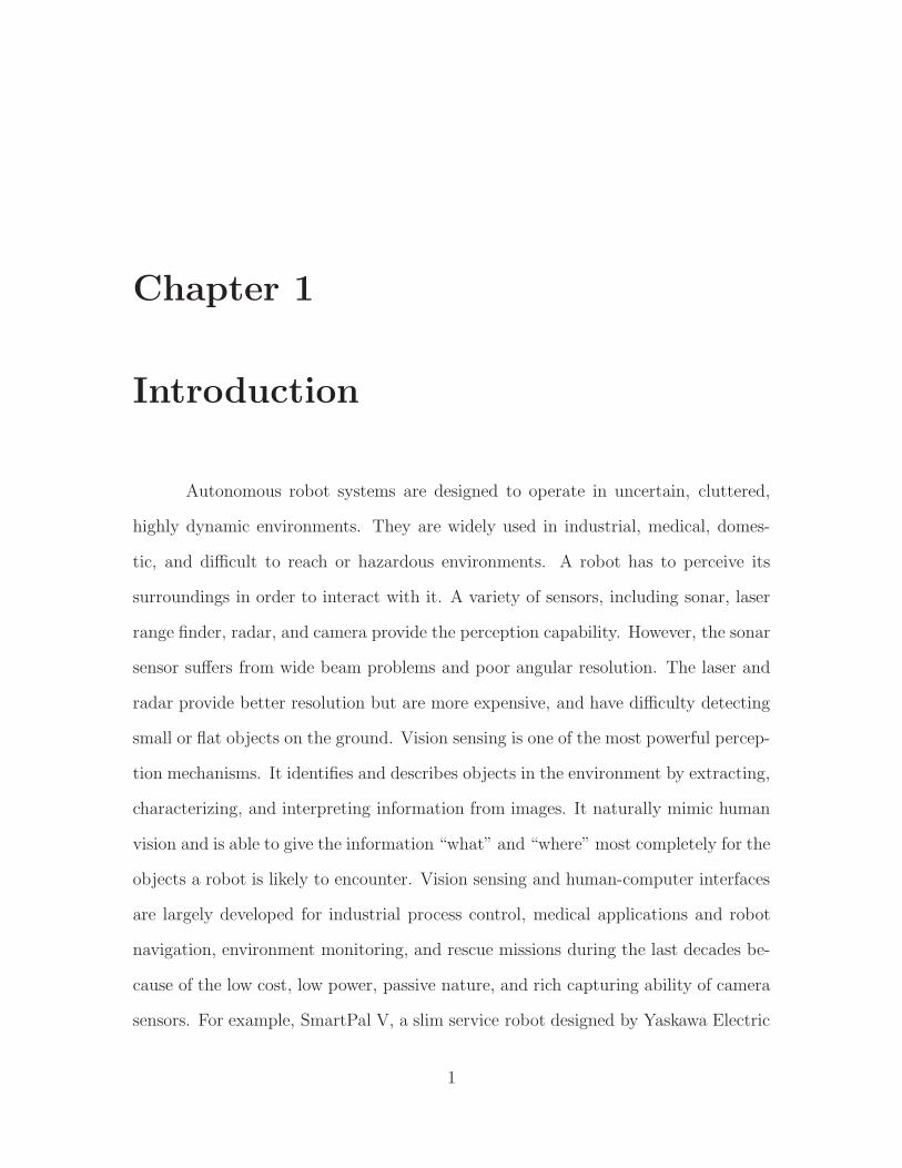
Figure 1.1: A typical example of path following. Top-left: The coordinates offeature points during the replay phase are compared with those obtained duringthe teaching phase in order to determine the turning direction. Top-right: Fea-tures obtained in the teaching phase. Bottom-left: The robot following a path.Bottom-left: Comparison of teaching and replay path.
autonomously follows that path in a replay phase. The coordinates of feature points
during the replay phase are compared with those obtained during the teaching phase
in order to determine the turning direction. Experimental results demonstrate the
capability of autonomous navigation in both indoor and outdoor environments, on
both flat and slanted surfaces, for distances over 200 meters. The technique requires
a single off-the-shelf, forward-looking camera with no calibration (either external or
internal, including lens distortion). The algorithm is entirely qualitative in nature,
requiring no map of the environment, no image Jacobian, no homography, no funda-
mental matrix, and no assumption about a flat ground plane. A typical example is
shown in Figure 1.1.
4

1.1.2 Person following
The ability to automatically follow a person is a key enabling technology for
mobile robots to effectively interact with the surrounding world. Numerous applica-
tions would benefit from such a capability, including security robots that detect and
follow intruders, interactive robots, and service robots that must follow a person to
provide continual assistance [75, 86, 90]. In our lab, we are particularly interested in
developing personal digital assistants for medical personnel in hospital environments,
providing physicians with ready access to charts, supplies, and patient data. Another
related application is that of automating time-and-motion studies for increasing the
clinical efficiency in hospitals [9].
Tracking people from a mobile platform is one of the least developed and more
difficult areas of machine vision. People are non-rigid objects and are difficult to model
geometrically; plus, the occlusions and distractions from the environment, including
other people, can confuse the tracker. And the foreground segmentation is more
difficult from a moving platform than from a fixed viewpoint because the background
undergoes motion relative to the platform, making static background subtraction
is not applicable. To keep up with a walking person in real-time, the detection and
tracking algorithm must be fast enough and require very quick focus of attention. The
most popular approach utilizes appearance properties, such as color, that distinguish
the target person from the surrounding environment. This method requires the person
to wear clothes that have a different color from the background. In addition, lighting
changes tend to cause serious problems for color-based techniques. Other researchers
have applied optic flow to the problem. These techniques are subject to drift as the
person moves about the environment, particularly with rotation, and are therefore
limited to short paths.
5
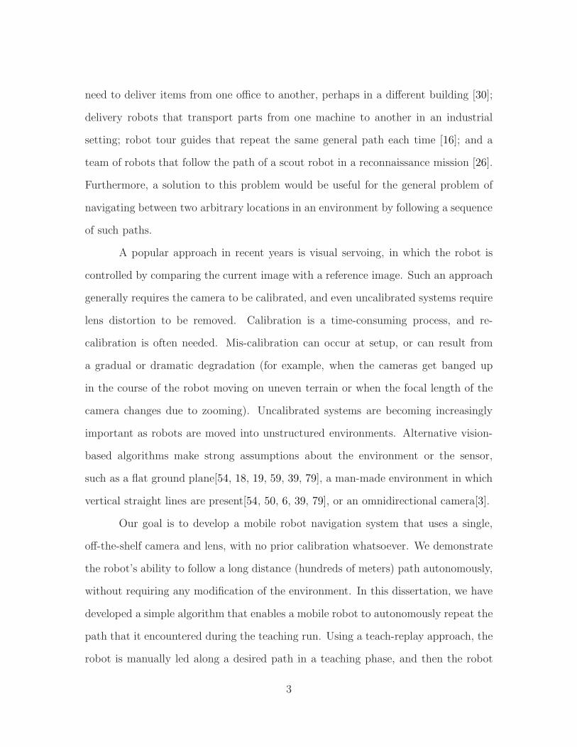
Figure 1.2: A typical example of person following. Left: A robot following a person.The person wears clothing with the same color as the environment. Right: Featuredetection and matching in order to extract the person.
We have developed an algorithm using feature detection and matching in order
to determine the location of the person in the image and thereby control the robot,
as shown in Figure 1.2. Motion and stereo information is fused in order to handle
difficult situations such as dynamic backgrounds and out-of-plane rotation. Unlike
color-based approaches, the person is not required to wear clothing with a different
color from the environment. Our system is able to reliably follow a person in complex
dynamic, cluttered environments in real time.
1.1.3 Door detection
Doors are important landmarks for indoor mobile robot navigation. They
mark the entrance/exit of rooms in many offices and laboratory environments. The
ability of a robot to detect doors can be a key point for a robust navigation. However,
there are still no fully operational systems that can operate robustly to detect doors
in various environments.
Recognizing doors involves dealing with many factors that may affect the
appearances of the objects: scale changes, perspective transformation of the door
6

appearance in the image plane, lighting conditions, partial occlusion, other similar
objects in the scene, etc. These factors make the door detection difficult. For ex-
amples, the color of the door might be the same as the wall; the floor might exhibit
high reflection that severely distract the detector; the doors may be located in differ-
ent geometrical positions and poses relative to the camera; and the drastic lighting
changes may occur between the environment and the door.
Much of the previous work on door detection has relied upon 3D range infor-
mation available from sonar, lasers, or stereo vision [47, 73, 89, 4]. We are interested,
however, in using off-the-shelf cameras for detecting doors, primarily because of their
low-cost, low-power, and passive sensing characteristics, in addition to the rich infor-
mation they provide. Figure 1.3 illustrates our scenario, as well as the difficulties of
solving this problem. The robot is equipped with two webcams, each one pointing
at a different side of the hallway as the robot drives. Because there is no overlap
between the cameras, stereo vision is not possible. Even more importantly, because
the cameras are low to the ground, the top of the door (the lintel) — which otherwise
would provide a powerful cue for aiding door detection — is often occluded by the top
of the image. Pointing the cameras upward is not possible, because of the importance
of being able to see the ground to avoid obstacles. Even with these constraints, our
goal is to detect doors in a variety of environments, containing textured and untex-
tured floors, walls and doors with similar colors, low-contrast edges, bright reflections,
variable lighting conditions, and changing robot pose, as shown in Figure 1.3.
We present an algorithm to detect doors in images. The key to the algorithm’s
success is its fusion of multiple visual cues, including standard cues (color, texture,
and intensity edges) as well as several novel ones (concavity, the kick plate, the vanish-
ing point, and the intensity profile of the gap below the door). We use the Adaboost
algorithm to ensure optimal linear weighting of the various cues. Formulated as a
7
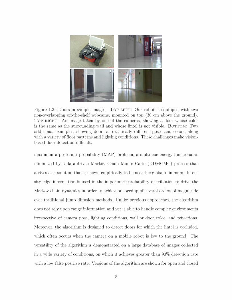
Figure 1.3: Doors in sample images. Top-left: Our robot is equipped with twonon-overlapping off-the-shelf webcams, mounted on top (30 cm above the ground).Top-right: An image taken by one of the cameras, showing a door whose coloris the same as the surrounding wall and whose lintel is not visible. Bottom: Twoadditional examples, showing doors at drastically different poses and colors, alongwith a variety of floor patterns and lighting conditions. These challenges make vision-based door detection difficult.
maximum a posteriori probability (MAP) problem, a multi-cue energy functional is
minimized by a data-driven Markov Chain Monte Carlo (DDMCMC) process that
arrives at a solution that is shown empirically to be near the global minimum. Inten-
sity edge information is used in the importance probability distribution to drive the
Markov chain dynamics in order to achieve a speedup of several orders of magnitude
over traditional jump diffusion methods. Unlike previous approaches, the algorithm
does not rely upon range information and yet is able to handle complex environments
irrespective of camera pose, lighting conditions, wall or door color, and reflections.
Moreover, the algorithm is designed to detect doors for which the lintel is occluded,
which often occurs when the camera on a mobile robot is low to the ground. The
versatility of the algorithm is demonstrated on a large database of images collected
in a wide variety of conditions, on which it achieves greater than 90% detection rate
with a low false positive rate. Versions of the algorithm are shown for open and closed
8
doors, as well as for calibrated and uncalibrated camera systems. Additional exper-
iments demonstrate the suitability of the algorithm for near-real-time applications
using a mobile robot equipped with off-the-shelf cameras.
1.2 Application scenario
The research of this dissertation would benefit many applications, especially in
the development of fully autonomous robots. In the future, the three algorithms pre-
sented could be integrated into a robot navigation system toward fully autonomous
robot applications. For example, autonomous robot is highly desired in the hospital
distribution service for decreasing operating costs while improving delivery perfor-
mance. To meet the delivery needs of a hospital, any automated solution will need to
handle routine deliveries as well as be flexible enough to handle arbitrary deliveries
or other exceptions to the norm [76]. For routine pick-ups and deliveries, the robot
follows a predefined route to deliver supplies to and from the service units. Beside
routine deliveries, sometime the robot needs to deliver items to specific rooms. There-
fore, door detection and recognition are required.1 For arbitrary deliveries, the robot
could follow a hospital staff to deliver emergent supplies anywhere as required.
1.3 Outline of dissertation
Following this introduction, the structure of this dissertation is a brief state
of the art concerning related work on three specific topics in Chapter 2: path fol-
lowing, person following and door detection. Also discussed are some issues in their
approaches. Then overviews of our approaches, and their advantages are described.
1Door recognition is not included in this dissertation.
9

This is followed by our qualitative vision-based path following algorithm, which is
presented in Chapter 3; after that, the motion-based person following algorithm is
presented in Chapter 4. Chapter 5 presents the door detection approach, including
detecting both open and closed doors and tracking doors in videos. Chapters 3, 4
and 5 comprise a significant portion of the thesis. Once each algorithm is described,
its applications to the mobile robot and the experimental results, and also the prac-
tical system limitations are given at the end of each Chapter. Finally, Chapter 6
presents some conclusions and suggestions for future work, along with a summary of
the contributions of the dissertation.
10
Chapter 2
Related Work
In Chapter 1 we discussed general problems existing in vision-based mobile
robot sensing regarding three topics: path following, person following, and door de-
tection. This chapter reviews previous research in each of these three areas. The
first section reviews previous research relevant to state-of-the-art path following ap-
proaches for long distance navigation in unstructured environments; particular em-
phasis is placed on the need for uncalibration systems. The second section reviews
previous work on person following, that is, how to extract a person from a cluttered
background and reliably track the person over time. In the third section a brief back-
ground of door detection is presented. The anatomy of the door is discussed along
with visual cues suitable for detecting doors in images. Brief introductions of our
solutions to existing problems are given at the end of each section.
2.1 Path following
Two questions that arise when addressing the path-following problem are
the representation for the destination location and the choice of sensor. A tra-
11
ditional answer to the former question has been to build and maintain a global
map of the environment, and to represent the destination as a point in that map
[17, 52, 56, 101, 93, 94, 5]. While a global map is needed to compute the global
location of the robot (particularly when its initial location is unknown), such a com-
plicated approach may not be necessary to simply follow an incremental path to the
destination [27]. Regarding the latter question, compared with other sensors vision is
a promising option due to its low cost, low power consumption, and passive sensing
[14]. Just as vision is a dominant sense in many biological systems, it is likely to
become increasingly important in robotic systems.
An approach that has been gaining popularity in recent years is visual servoing,
in which the robot is controlled by comparing the current image with a reference
image, both taken by a camera on the robot [44, 22]. These techniques generally use a
Jacobian that relates the coordinates of points in the world with their projected image
coordinates [18]. Alternatively, some approaches utilize a homography or fundamental
matrix to relate the coordinates between images [79, 59]. Vision-based algorithms
usually make strong assumptions about the sensor or the environment, such as a
calibrated camera (even uncalibrated systems often require some sort of calibration,
such as removing lens distortion) [18, 6, 19], a flat ground plane [54, 18, 19, 59, 39, 79],
or a man-made environment in which vertical straight lines [54, 50, 6, 39, 79] or the
flat, parallel walls of a corridor are present [80]. Some systems require two or more
cameras [52, 6, 85] or omnidirectional cameras [3], which are not as readily available
as standard monocular cameras.
To some extent, map-based approaches using calibrated cameras have made
significant progress in path following. Royer et al. [78] built a monocular vision
mobile robot system, which probably is the one of the most successful approaches.
The robot is equipped with a wide angle camera in a front looking position. A
12

video sequence acquired in the learning step is processed off line to build a map of
the environment with a structure-from-motion algorithm. Then the robot is able to
follow the same path as in the learning step in real time. However, the camera has
to be well calibrated and the ground is assumed locally planar and horizontal at the
current position of the robot.
To overcome these limitations, we consider the problem from a novel view-
point in which there is no equation relating image coordinates to world coordinates.
Such a direct approach is motivated by the observation that the problem is vastly
overdetermined, with tens of thousands of image pixels available to determine a single
turning command output. In Chapter 3, we present a simple algorithm that uses a
single, off-the-shelf camera attached to the front of the robot. The technique follows
the teach-replay approach [18] in which the robot is manually led through the path
once during a teaching phase and then follows the path autonomously during the
replay phase. Without any camera calibration (even calibration for lens distortion),
the robot is able to follow the path by making only qualitative comparisons between
the feature coordinates in the two phases. All that is needed is a single controller
gain parameter to convert pixel coordinates to turning angles. We demonstrate the
technique on several indoor and outdoor experiments, showing its robustness with
respect to slanted surfaces, changing lighting conditions, and dynamic occluding ob-
jects. This paper extends the applicability and improves upon the robustness of our
earlier work [23] by incorporating odometry information and correcting for camera
roll. We also demonstrate the ability of the technique to work with wide-angle and
omnidirectional cameras, with only slight modification in the latter case to ignore the
bottom half of the image which views the scene behind the robot.
The proposed approach falls within the category of mapless algorithms [27]. As
such, it is closely related to the view-sequenced route representation (VSRR) of Mat-
13

sumoto et al. [62, 63, 45] in which the turning angle is computed by cross-correlating
images acquired during the replay phase with those captured during training. How-
ever, VSRR requires large amounts of memory to store the views and is sensitive
to occlusions by dynamic objects. Along with a homography-based extension using
vertical lines [79], it has only been demonstrated for short sequences on flat terrains.
An alternate mapless approach is to learn the mapping from images to turning
commands based on their classification [99, 2]. While this method can successfully
follow a specific pattern such as a road or hallway, it will have difficulty generalizing
to environments in which the images cannot be categorized into a small number of
classes known at training time. Another approach that has received considerable
attention [37, 100, 102, 87, 51, 97, 43] is to store an example image with each specific
location of interest. At run time, the image database is searched to find the image
that most closely resembles the current one (or, alternatively, the current image is
projected onto a manifold learned from the database [70, 53]). Such approaches
require extensive training and have difficulty providing sufficient spatial resolution to
determine actual turning commands in large environments. Similarly, sensory-motor
learning has been used to map visual inputs to turning commands, but the resulting
algorithms have been too computationally demanding for real-time performance [38].
Other researchers have developed mapless algorithms for low-level functionality like
corridor following or obstacle avoidance [72, 80, 10, 57, 65, 69], but these techniques
are not applicable to following a specific arbitrary path.
2.2 Person following
Existing approaches to vision-based person following can be classified into
three categories. First, the most popular approach is to utilize appearance properties
14
that distinguish the target person from the surrounding environment. For example,
Sidenbladh et al. [86] segment the image using binary skin color classification to
determine the pixels belonging to the face. Similarly, Tarokh and Ferrari [91] use
the clothing color to segment the image, applying statistical tests to the resulting
blobs to find the person. Schlegel et al. [81] combine color histograms with an edge-
based module to improve robustness at the expense of greater computation. More
recently, Kwon et al. [55] use color histograms to locate the person in two images, then
triangulate to yield the distance. One limitation of these methods is the requirement
that the person wear clothes that have a different color from the background. In
addition, they are sensitive to illumination changes.
Other researchers have applied optical flow to the problem. An example of
this approach is that of Piaggio et al. [75], in which the optical flow is thresholded
to segment the person from the background by assuming that the person moves
differently from the background. Chivilo et al. [36] use the optical flow in the center
of the image to extract velocity information, which is viewed as a disturbance to be
minimized by regularization. These techniques are subject to drift as the person moves
about the environment, particularly with out-of-plane rotation, and are therefore
limited to short paths.
As a third approach, Beymer and Konolige [11] use dense stereo matching to
reconstruct a 2D plan view of the objects in the environment. Odometry information
is applied to estimate the motion of the background relative to the robot, which
is then used to perform background subtraction in the plan view. The person is
detected as the object that remains after the segmentation, and a Kalman filter is
applied to maintain the location of the person. One of the complications arising from
background subtraction is the difficulty of predicting the movement of the robot due
to uneven surfaces, slippage in the wheels, and the lack of synchronization between
15

encoders and cameras.
In Chapter 4 an approach based upon matching sparse Lucas-Kanade fea-
tures [84, 95] in a binocular stereo system is presented. The algorithm, which we
call Binocular Sparse Feature Segmentation (BSFS), involves detecting and matching
feature points both between the stereo pair of images and between successive im-
ages of the video sequence. Random Sample Consensus (RANSAC) [32] is applied to
the matched points in order to estimate the motion model of the static background.
Stereo and motion information are fused in a novel manner in order to segment the
independently moving objects from the static background by assuming continuity of
depth and motion from the previous frame. The underlying assumption of the BSFS
algorithm is modest, namely, that the disparity of the features on the person should
not change drastically between successive frames.
Because the entire technique uses only gray-level information and does not
attempt to reconstruct a geometric model of the environment, it does not require
the person to wear a distinct color from the background, and it is robust to having
other moving objects in the scene. Another advantage of using sparse features is
that the stereo system does not need to be calibrated, either internally or externally.
The algorithm has been tested in cluttered environments in difficult scenarios such
as out-of-plane rotation, multiple moving objects, and similar disparity and motion
between the person and the background.
2.3 Door Detection
Some researchers have developed door detection systems using only range in-
formation, without cameras. Early work involved sonar sensors [74], while more recent
work utilizes laser range finders [8, 64]. In all of these approaches, the detector re-
16

quires the door plane to be distinguishable from the wall plane either because the
door is recessed, a molding protrudes around the door, or the door is slightly open.
Thus, if a door is completely flush with the wall, such detectors will be unable to find
it.
Perhaps the most popular approach to door detection involves combining range
sensors with vision. Kim and Nevatia [47] extract both vertical (post) and horizon-
tal (lintel) line segments from an image, then analyze whether these segments meet
minimum length and height restrictions, verifying door candidates by a 3D trinocular
stereo system. Stoeter et al. [89] extract vertical lines in the image using the Sobel
edge detector followed by morphological noise removing, then combine the resulting
lines with range information from a ring of sonars to detect doors. In contrast, the
system of Anguelov et al. [4] does not use intensity edges at all but rather the colors
along a single scan of an omnidirectional image combined with a laser range finder.
Doors are first detected by observing their motion over time (i.e., whether an open
door later becomes closed, or vice versa) in order to learn a global mean door color.
Doors are then detected in an expectation-maximization framework by combining the
motion information with the door width (as estimated by the laser range finder) and
the similarity of image data to the learned door color. This approach assumes that
the doors are all similarly colored, and that the mean color of the doors and walls
are significantly different from each other. Another piece of interesting research is
that of Hensler et al. [42], who augment our recent vision-only algorithm [24] with
a laser range finder to estimate the concavity and width of the door, which are then
combined with other image-based features.
A few researchers have focused upon the much more difficult problem of de-
tecting doors using vision alone, without range information. Monasterio et al. [67]
detect intensity edges corresponding to the posts and then classify the scene as a door
17

if the column between the edges is wider than a certain number of pixels, an approach
that assumes a particular orientation and distance of the robot to the door. Similarly,
Munoz-Salinas et al. [68] apply fuzzy logic to establish the membership degree of an
intensity pattern in a fuzzy set using horizontal and vertical line segments. Rous et
al. [77] generate a convex polygonal grid based on extracted lines, and they define
doors as two vertical edges that intersect the floor and extend above the center of
the image. Their work employs mean color information to segment the floor, thus
assuming that the floor is not textured. An alternate approach by Cicirelli et al. [25]
analyzes every pixel in the image using two neural networks: one to detect the door
corners, and one to detect the door frame, both of which are applied to the hue and
saturation color channels of the image.
While these previous systems have achieved some success, no vision-only sys-
tem has yet demonstrated the capability of handling a variety of challenging environ-
mental conditions (changing pose, similarly colored doors and walls, strong reflections,
and so forth) in the presence of the lintel-occlusion that often occurs when the camera
is low to the ground and the door is nearby.
In Chapter 5 we present a solution to the problem based upon combining
multiple cues. Our approach augments standard features such as color, texture,
and vertical intensity edges with novel geometric features such as the concavity of
the door and the gap below the bottom door edge. The approach builds on our
previous research [24] by incorporating these features into a maximum a posteriori
(MAP) framework. Adaboost [33] is used to compute the optimal linear weighting of
the different features, and a Data Driven Markov Chain Monte Carlo (DDMCMC)
technique is used to explore the solution space. By incorporating intensity edges in
the importance proposal distribution, a significant speedup is achieved in comparison
to the traditional jump diffusion methods. We also present variations of the algorithm
18

for detecting open as well as closed doors, and for working with calibrated as well
as uncalibrated camera systems. Experimental results on a large database of images
show the versatility of the algorithm in detecting doors in a variety of challenging
environmental conditions, achieving a nearly global optimal solution in many cases.
We also incorporate the algorithm into a real-time system that detects doors as the
robot drives down a corridor.
19
Chapter 3
Path Following
Visual path following is a method that a robot can autonomously repeat a
previous path to a given location. Cartwright and Collett [21] believe that the path
following behavior can be achieved without a topographical map. They propose a
“snapshot” model, which is designed to explain how a bee might return to a goal
using a two-dimensional “snapshot” of the landscape seen from the goal. To guide
its return, the bee continuously compares its snapshot with its current retinal image
and moves so as to reduce the discrepancy between the two. Bees can only be guided
in the right direction by the difference between current retinal image and snapshot
when there is some resemblance between the two.
As Burschka and Hager [18] insightfully point out, the problem of following a
predetermined path may not require a complicated approach. Intuitively, the vastly
overdetermined nature of the problem (thousands of pixels in an image versus one
turning command output) would seem to indicate that a simple method might be
feasible. In this chapter we present a simple qualitative path following algorithm
relying on visual tracking of features (landmarks). The technique follows the teach-
replay approach [18] in which the robot is manually led through the path once during
20
a teaching phase and then follows the path autonomously during the replay phase.
Without any camera calibration (even calibration for lens distortion), the robot is
able to follow the path by making only qualitative comparisons between the feature
coordinates in the two phases.
Section 3.1 presents the qualitative feature mapping method for path following,
including a novel concept called the funnel lane and the control algorithm . Section 3.2
briefly introduces how to select and track features. Section 3.3 describes the detailed
strategy of teach-and-replay using qualitative feature mapping. Experimental results
including indoor and outdoor are given in Section 3.4. Finally, Section 3.5 presents
the conclusions.
3.1 Qualitative mapping from feature coordinates
to turning direction
Consider a mobile robot equipped with a camera whose optical axis is paral-
lel to the heading direction of the robot. Suppose we wish to move the robot from
location C = (xC , yC , θC ) to a previously encountered location D = (xD , yD , θD),
where (xi , yi) and θi are the position and orientation, respectively, in the xy plane,
i ∈ {C ,D}. The robot has access to a current image IC , taken at C , and a destination
image ID , taken previously at the destination D . In this section we introduce a quali-
tative test on image feature coordinates that guides the robot toward the destination.
We start with a simple observation. Suppose the robot views a fixed landmark in
both images yielding image feature coordinates of uC and uD , as shown in Figure
3.1. The features are computed with respect to a coordinate system centered at the
principal point (the intersection of the optical axis and the image plane), so that
21
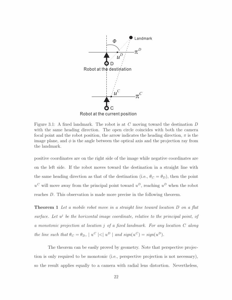
Figure 3.1: A fixed landmark. The robot is at C moving toward the destination Dwith the same heading direction. The open circle coincides with both the camerafocal point and the robot position, the arrow indicates the heading direction, π is theimage plane, and φ is the angle between the optical axis and the projection ray fromthe landmark.
positive coordinates are on the right side of the image while negative coordinates are
on the left side. If the robot moves toward the destination in a straight line with
the same heading direction as that of the destination (i.e., θC = θD), then the point
uC will move away from the principal point toward uD , reaching uD when the robot
reaches D . This observation is made more precise in the following theorem.
Theorem 1 Let a mobile robot move in a straight line toward location D on a flat
surface. Let u j be the horizontal image coordinate, relative to the principal point, of
a monotonic projection at location j of a fixed landmark. For any location C along
the line such that θC = θD , | uC |<| uD | and sign(uC ) = sign(uD).
The theorem can be easily proved by geometry. Note that perspective projec-
tion is only required to be monotonic (i.e., perspective projection is not necessary),
so the result applies equally to a camera with radial lens distortion. Nevertheless,
22

we will assume perspective projection throughout this section to simplify the presen-
tation. Although the assumption of a flat surface is needed in theory, it has little
effect in practice. A non-zero tilt angle has negligible effect on horizontal coordinates.
We apply the random sample consensus (RANSAC) algorithm to compensate the roll
angle and therefore align the the teaching images and the replay images.
3.1.1 The funnel lane
According to the preceding theorem, if the robot is on the path toward the
destination with the same heading direction, then two constraints are satisfied. We
call these the funnel constraints. Conversely, as shown in Figure 3.2, if the constraints
are satisfied then the robot lies within a trapezoidal region for any given relative robot
angle α = θC − θD . For α = 0 the sides of the trapezoid are defined by two lines
passing through the landmark, one through D and another that is parallel to the
destination direction. These lines are rotated about the landmark by α if the relative
angle is nonzero. We call the trapezoidal region the funnel lane associated with the
landmark, destination, and relative angle. The terminology arises from the analogy
of pouring liquid into a funnel: The liquid moves in a straight line until it hits the
sides of the funnel, which cause it to bounce back and forth until it eventually reaches
the spout. In a similar manner, the sides of the trapezoid act as bumpers, guiding
the robot toward the goal. The notion of the funnel and the funnel lane are captured
in the following definitions.
Definition 1 The funnel of a fixed landmark λ and a robot location D is the set of
locations Fλ,D such that, for each C ∈ Fλ,D , the two funnel constraints are satisfied:
| uC | < | uD | (Constraint 1)
23

sign(uC ) = sign(uD) (Constraint 2)
where uC and uD are the coordinates of the image projection of λ at the locations C
and D, respectively.
Definition 2 The funnel lane of a fixed landmark λ, a robot location D, and a relative
angle α is the set of locations Fλ,D ,α ⊂ Fλ,D such that θC − θD = α for each C ∈
Fλ,D ,α.
Figure 3.2: The funnel lane with a fixed landmark. The funnel lane created by thetwo constraints, shown when the robot is facing the correct direction (left) and whenit has turned by an angle α (right).
Multiple features yield multiple funnel lanes, the intersection of which is the
set of locations for which both constraints are satisfied for all the features. This
intersection, which we call the combined funnel lane, is depicted in Figure 3.3. Notice
the importance of having features on both sides of the image in order to narrowly
constrain the path of the robot, thus achieving more robust and accurate results.
24

Figure 3.3: The combined funnel lane created by multiple landmarks. The combinedfunnel lane created by multiple feature points, shown when the robot is facing thecorrect direction (left) and when it has turned by an angle α (right).
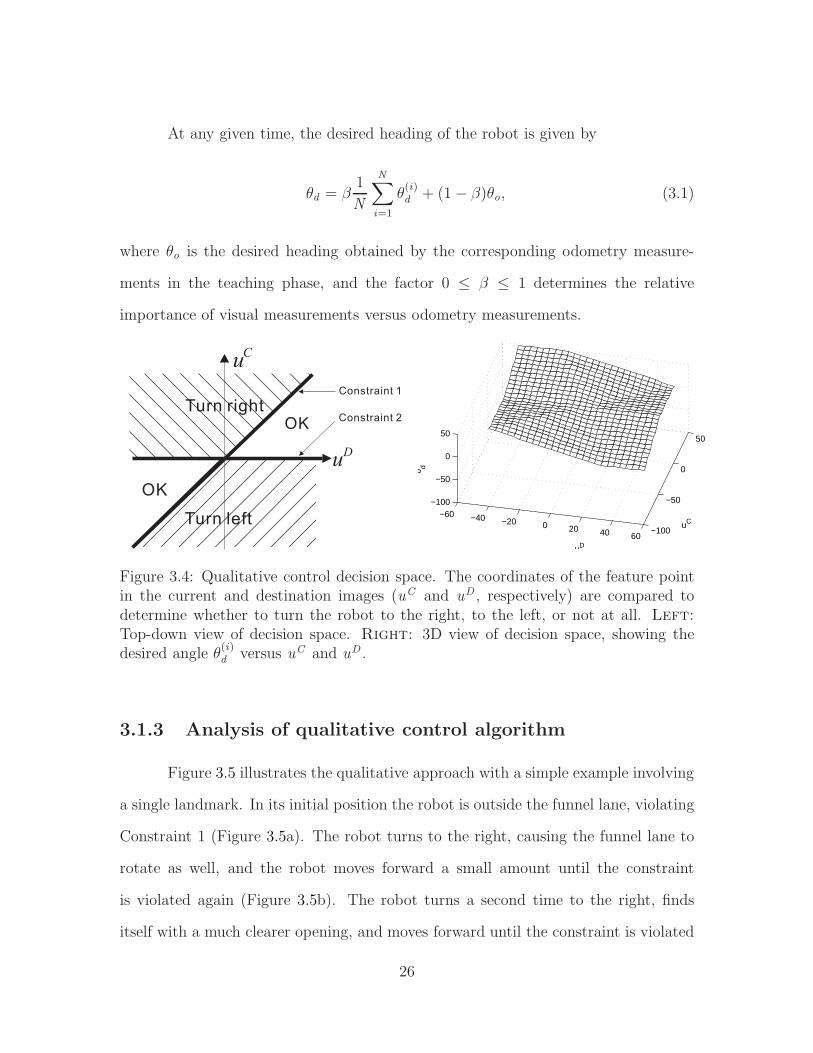
3.1.2 Qualitative control algorithm
The funnel constraints lead to a simple control algorithm, illustrated in Fig-
ure 3.4. The robot continually moves forward, turning to the right whenever Con-
straint 1 is violated and to the left whenever Constraint 2 is violated, given a feature
on the right side of the image (uD > 0). If the feature is on the left side (uD < 0),
then the directions are reversed.
For each feature i , a desired heading is obtained by
θ(i)d =
γ min{uC , φ(uC , uD)} if uC > 0 and uC > uD
γ max{uC , φ(uC , uD)} if uC < 0 and uC < uD
0 otherwise
where φ(uC , uD) = sgn(uC − uD)√
12(uC − uD)2 is the signed distance to the line
uC = uD . Here we approximate the conversion of pixels to radians with a constant
gain γ, but more involved mappings could be used.
25
At any given time, the desired heading of the robot is given by
θd = β1
N
N∑
i=1
θ(i)d + (1− β)θo, (3.1)
where θo is the desired heading obtained by the corresponding odometry measure-
ments in the teaching phase, and the factor 0 ≤ β ≤ 1 determines the relative
importance of visual measurements versus odometry measurements.
−60 −40 −20 0 20 40 60−100
−50
0
50
−100
−50
0
50
uC
uD
θ d(i)
Figure 3.4: Qualitative control decision space. The coordinates of the feature pointin the current and destination images (uC and uD , respectively) are compared todetermine whether to turn the robot to the right, to the left, or not at all. Left:
Top-down view of decision space. Right: 3D view of decision space, showing thedesired angle θ
(i)d versus uC and uD .
3.1.3 Analysis of qualitative control algorithm
Figure 3.5 illustrates the qualitative approach with a simple example involving
a single landmark. In its initial position the robot is outside the funnel lane, violating
Constraint 1 (Figure 3.5a). The robot turns to the right, causing the funnel lane to
rotate as well, and the robot moves forward a small amount until the constraint
is violated again (Figure 3.5b). The robot turns a second time to the right, finds
itself with a much clearer opening, and moves forward until the constraint is violated
26
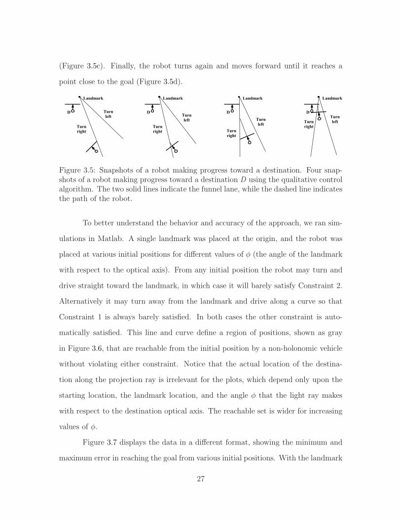
(Figure 3.5c). Finally, the robot turns again and moves forward until it reaches a
point close to the goal (Figure 3.5d).
Figure 3.5: Snapshots of a robot making progress toward a destination. Four snap-shots of a robot making progress toward a destination D using the qualitative controlalgorithm. The two solid lines indicate the funnel lane, while the dashed line indicatesthe path of the robot.
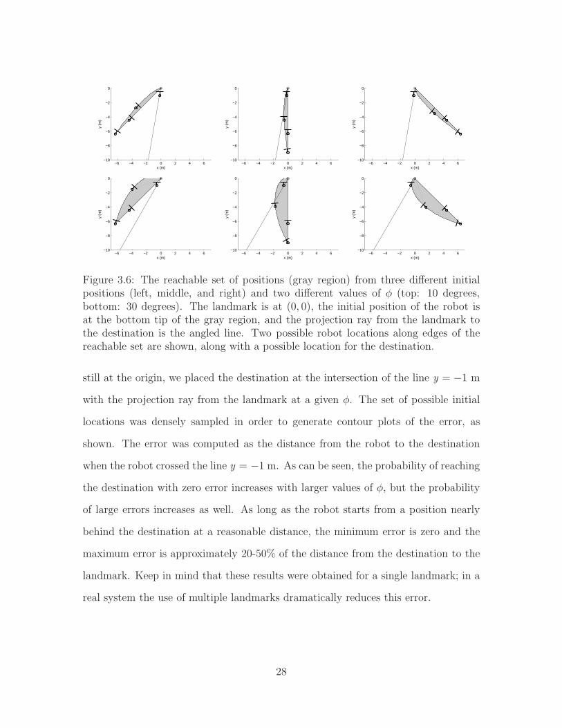
To better understand the behavior and accuracy of the approach, we ran sim-
ulations in Matlab. A single landmark was placed at the origin, and the robot was
placed at various initial positions for different values of φ (the angle of the landmark
with respect to the optical axis). From any initial position the robot may turn and
drive straight toward the landmark, in which case it will barely satisfy Constraint 2.
Alternatively it may turn away from the landmark and drive along a curve so that
Constraint 1 is always barely satisfied. In both cases the other constraint is auto-
matically satisfied. This line and curve define a region of positions, shown as gray
in Figure 3.6, that are reachable from the initial position by a non-holonomic vehicle
without violating either constraint. Notice that the actual location of the destina-
tion along the projection ray is irrelevant for the plots, which depend only upon the
starting location, the landmark location, and the angle φ that the light ray makes
with respect to the destination optical axis. The reachable set is wider for increasing
values of φ.
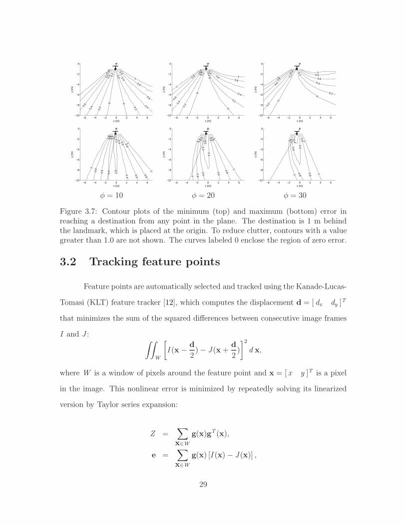
Figure 3.7 displays the data in a different format, showing the minimum and
maximum error in reaching the goal from various initial positions. With the landmark
27
−6 −4 −2 0 2 4 6−10
−8
−6
−4
−2
0
x (m)
y (m
)
−6 −4 −2 0 2 4 6−10
−8
−6
−4
−2
0
x (m)
y (m
)
−6 −4 −2 0 2 4 6−10
−8
−6
−4
−2
0
x (m)
y (m
)
−6 −4 −2 0 2 4 6−10
−8
−6
−4
−2
0
x (m)
y (m
)
−6 −4 −2 0 2 4 6−10
−8
−6
−4
−2
0
x (m)
y (m
)
−6 −4 −2 0 2 4 6−10
−8
−6
−4
−2
0
x (m)
y (m
)
Figure 3.6: The reachable set of positions (gray region) from three different initialpositions (left, middle, and right) and two different values of φ (top: 10 degrees,bottom: 30 degrees). The landmark is at (0, 0), the initial position of the robot isat the bottom tip of the gray region, and the projection ray from the landmark tothe destination is the angled line. Two possible robot locations along edges of thereachable set are shown, along with a possible location for the destination.
still at the origin, we placed the destination at the intersection of the line y = −1 m
with the projection ray from the landmark at a given φ. The set of possible initial
locations was densely sampled in order to generate contour plots of the error, as
shown. The error was computed as the distance from the robot to the destination
when the robot crossed the line y = −1 m. As can be seen, the probability of reaching
the destination with zero error increases with larger values of φ, but the probability
of large errors increases as well. As long as the robot starts from a position nearly
behind the destination at a reasonable distance, the minimum error is zero and the
maximum error is approximately 20-50% of the distance from the destination to the
landmark. Keep in mind that these results were obtained for a single landmark; in a
real system the use of multiple landmarks dramatically reduces this error.
28
−6 −4 −2 0 2 4 6−10
−8
−6
−4
−2
0
x (m)
y (m
)
0
0
0
0.2
0.2 0.2
0.20.4
0.4 0.4
0.40.
6
0.6
0.6
0.6
0.8
0.8
1
1
−6 −4 −2 0 2 4 6−10
−8
−6
−4
−2
0
x (m)
y (m
)
00
00.2
0.2 0.2
0.2
0.4
0.4
0.4
0.4
0.6
0.6
0.60.80.8
1
1
−6 −4 −2 0 2 4 6−10
−8
−6
−4
−2
0
x (m)
y (m
)
0
0
0
0.2
0.2
0.2
0.2
0.4
0.40.6
0.60.80.8
1
1
−6 −4 −2 0 2 4 6−10
−8
−6
−4
−2
0
x (m)
y (m
)
0.2
0.20.2
0.4
0.4
0.4
0.4
0.6
0.6
0.6
0.6
0.8
0.8
0.8
0.8
1
1
1
1
−6 −4 −2 0 2 4 6−10
−8
−6
−4
−2
0
x (m)
y (m
)
0.20.4
0.40.
60.6
0.6
0.60.8
0.8
0.8
0.8
1
1
1
1
−6 −4 −2 0 2 4 6−10
−8
−6
−4
−2
0
x (m)
y (m
)
0.40.6
0.6
0.8
0.80.8
0.8
1
1
1
1
φ = 10 φ = 20 φ = 30
Figure 3.7: Contour plots of the minimum (top) and maximum (bottom) error inreaching a destination from any point in the plane. The destination is 1 m behindthe landmark, which is placed at the origin. To reduce clutter, contours with a valuegreater than 1.0 are not shown. The curves labeled 0 enclose the region of zero error.
3.2 Tracking feature points
Feature points are automatically selected and tracked using the Kanade-Lucas-
Tomasi (KLT) feature tracker [12], which computes the displacement d = [ dx dy ]T
that minimizes the sum of the squared differences between consecutive image frames
I and J : ∫∫
W
[I (x− d
2)− J (x +
d
2)
]2
d x,
where W is a window of pixels around the feature point and x = [ x y ]T is a pixel
in the image. This nonlinear error is minimized by repeatedly solving its linearized
version by Taylor series expansion:
Z =∑
x∈W
g(x)gT (x),
e =∑
x∈W
g(x) [I (x)− J (x)] ,
29

where g(x) = 12∂[I (x) + αJ (x)]/∂x is the spatial gradient of the weighted average
image. These equations are the standard Lucas-Kanade equations [61, 7, 84, 95] with
geometric symmetry between the two images and an affine model of brightness to
model the dynamic lighting conditions encountered by the mobile robot, particularly
when moving outdoors [61, 71]. A coarse-to-fine pyramidal strategy is used to allow
large image motions. As in [84, 95], features are automatically selected as those
points in the image for which both eigenvalues of Z are greater than a specified
minimum threshold. This feature selection mechanism is a slight variation of the
Harris corner detector which has been shown to be effective for both its repeatability
rate, information content, and theoretical properties [40, 82, 46, 60].
The tracking algorithm just described relies on the well-known constant bright-
ness assumption [96] in which image intensities are constant over time. As a robot
moves about a real environment, however, the lighting conditions often change from
one location to another. This problem is particularly acute in outdoor scenes during
daylight hours when the robot moves in and out of shadows or when the sun is oc-
cluded or disoccluded by clouds. In such scenarios the standard algorithm often loses
feature points prematurely. We present a simple extension of the KLT algorithm to
handle illumination changes.
The residue equation defined above is augmented with a relative gain α and
bias β describing the illumination relationship between the two images:
∫∫
W
[I (x− d
2)−
(αJ (x +
d
2) + β
)]2
d x.
Applying a Taylor series expansion as above yields similar equations:
Z =∑
x∈W
g(x)gT (x),
30

e =∑
x∈W
g(x) [I (x)− (αJ (x) + β)] ,
where g(x) = 12∂[I (x) + αJ (x)]/∂x.
The values α and β are computed separately for each window by solving the
following two equations:
E (I ) = αE (J ) + β
E (I 2) = α2E (J 2),
where E (I ) is the mean intensity of the pixels in the window and E (I 2) is the mean
squared intensity of the pixels in the window. Similarly for E (J ) and E (J 2).
3.3 Teach-and-replay navigation
The navigation system involves two phases. In the teaching phase, an operator
manually moves the robot along a desired path to gather training data. The path
is divided into a number of non-overlapping segments defined by a constant amount
of travel time between them. Within each segment, feature points are automatically
detected in the first image and tracked throughout subsequent images. For each fea-
ture that is successfully tracked throughout a segment, its graylevel intensity pattern
and x -coordinate in the first and last images of the segment are stored in a database
for use in the replay phase. We also store the length of each segment and the change
of heading direction of the robot in each segment by odometry, which are used in
determining the segment transitions.
In the replay phase, the robot is manually placed in approximately the same
initial location as that of the teaching phase, and the robot proceeds sequentially
31

through the segments. At the beginning of each segment, the KLT algorithm is used
to establish correspondence between feature points in the current image and those
of the first teaching image of the segment. Then, as the feature points are tracked
in the incoming images, their coordinates are compared with those of the milestone
image (i.e., the last teaching image of the segment) in order to determine the turning
direction for the robot.
When the robot runs on an unpaved rough terrain, it moves from side to side
resulting in rotations in the image plane between the teaching and the replay images,
which give rise to incorrect funnel lanes. We apply the random sample consensus
(RANSAC) algorithm to align the teaching and replay images. We repeatedly pick
two random features in the milestone image and corresponding features in the replay
image and calculate the rotation angle, which is then applied to all the milestone
features to record the number of inliers. This process is repeated several times, and
the rotation model with the largest number of inliers is taken to be the rotation
between the teaching images and replay images.
A crucial component of the technique is determining when to transition to
a new segment. One approach would be to threshold the mean squared error of
the coordinates between the current and the milestone feature points. As the robot
approaches the milestone, this error should decrease. However, we have found it
impossible to find a single threshold that works in all environments, due to the various
sources of noise occurring in real video data. Instead, we rely on the fact that the mean
squared error tends to decrease over time as the robot approaches the milestone, then
increase afterward. Although this method works with visual data alone, we have
found a significant improvement in reliability when combining visual features with
odometric information. Because odometers are accurate along short distances, they
provide a healthy complement to the visual sensor whose strength is in the global
32
information that it provides. This global picture, in turn, complements the odometry
readings that drift over time due to slippage in the wheels and integration errors.
Thus, we continually monitor the value
δ = exp
{−
ǫ2f
2σ2f
}exp
{− ǫ2
o
2σ2o
}exp
{− ǫ2
h
2σ2h
}(3.2)
which estimates the likelihood that the robot is at the end of the current segment.
In this equation ǫf is the mean squared error of the feature coordinates between the
current and milestone images; ǫo is the difference between the distance traveled in
the current segment and the corresponding segment in the teaching phase, calculated
by odometry; and ǫh is the difference between the current heading and the heading
at the end of the teaching segment. These errors are normalized by values computed
automatically by the system: σf is the mean squared error of the feature points at the
beginning of the segment; σo is the length of the segment calculated by odometry in
the teaching phase; and σh is the maximum variation in heading encountered during
the teaching segment.
Due to the distraction from noise, δ might not decrease or increase mono-
tonically. We monitor the changes of δ between 5 consecutive frames. In these 5
consecutive frames, if most δ increase, the algorithm transitions to the next mile-
stone. At the same time, we also monitor δ changes in the previous segment and the
next segment. δ should always increase in the previous segment and decrease in the
next segment. Otherwise, the algorithm will transit back and forth.
33

3.4 Experimental results
The qualitative algorithm was implemented in Visual C++ on a Dell Inspiron
700m laptop (1.6 GHz) controlling an ActivMedia Pioneer P3-AT mobile robot with
an inexpensive Logitech QuickCam Pro 4000 webcam mounted on the front. The
320× 240 images were acquired at 30 Hz and processed by the KLT algorithm with
the default 7 × 7 feature window size [12]. In all experiments a maximum of 60
features were detected and tracked throughout each segment. On average 85% of the
features survive the initial correspondence in the first image of the segment during
replay. The algorithm was tested in a number of indoor and outdoor environments.1
3.4.1 Indoor experiments
The algorithm was tested in an indoor environment, including our laboratory
as well as a corridor of the hallway in our building. The maximum speed of the robot
during the teaching phase was 100 mm/s and the turning speed was 4 degrees per
second. Due to the small environment, the driving speed during the playback phase
was reduced in order to avoid going off course. Figure 3.8 shows a typical run in
which the robot successfully navigated between chairs and desks in our lab along a
10 m path. Trajectories displayed in the figure were computed by integrating the
odometry readings (which are not used by the algorithm). The maximum error was
0.35 m (for 80% of the path the error was less than 0.2 m), and the final error was
0.03 m.
Figure 3.9 shows the decision process at two time instants during the replay
phase. In one case the robot is pointing to the right of the current direction, so the
features on the left half of the image violate either Constraint 1 or Constraint 2,
1Videos of the results can be found at
http://www.ces.clemson.edu/~stb/research/mobile robot
34

0 1 2 3 4 5 6
−4
−3
−2
−1
0
1
x(m)
y(m
)
teachingreplay
DeskChair
Chair Chair Chair
Chair Chair Chair
Chair Chair Chair Chair
Desk
DeskDesk
Chair
Desk
Chair Cabinet
Door
Chair
a b c
0 2 4 6 8 10 12 140
0.05
0.1
0.15
0.2
0.25
0.3
0.35
erro
r(m
)
traveling distance(m)
Figure 3.8: Indoor navigation. Top: The teaching and replay paths of the robotin an indoor environment (our laboratory). The locations a, b, and c are used inFigure 3.10. Bottom: Error versus distance traveled.
thereby indicating the need for the robot to turn left. In the other case the features
on the right half of the image violate one of the constraints, thereby indicating the
need to turn right. In both cases notice the unanimity of the voting: Although many
features simply plead ignorance, those features that do cast a vote are in agreement.
Figure 3.10 displays the decision process during three segments of the ex-
periment. For display purposes, the feature coordinates are normalized so that the
interval y ∈ [0, 1] indicates “do not turn”, while larger values (y > 1) indicate “turn
right”, and smaller values (y < 0) indicate “turn left”, where y is defined as
y =
{1 + ut
i /∣∣ud
i
∣∣ (udi < 0)
uti /∣∣ud
i
∣∣ (udi > 0)
. (3.3)
Notice again the near unanimity in voting (a lone feature in (b) votes incorrectly to
turn left). Also notice that, as the robot turns (in (b) and (c)) the features move
toward the OK region.
Indoor environments present a particular challenge for feature point tracking
because of the lack of texture on the walls. Occasionally the robot fails to remain
on course due to lack of texture in the scene that causes feature points to be lost.
35
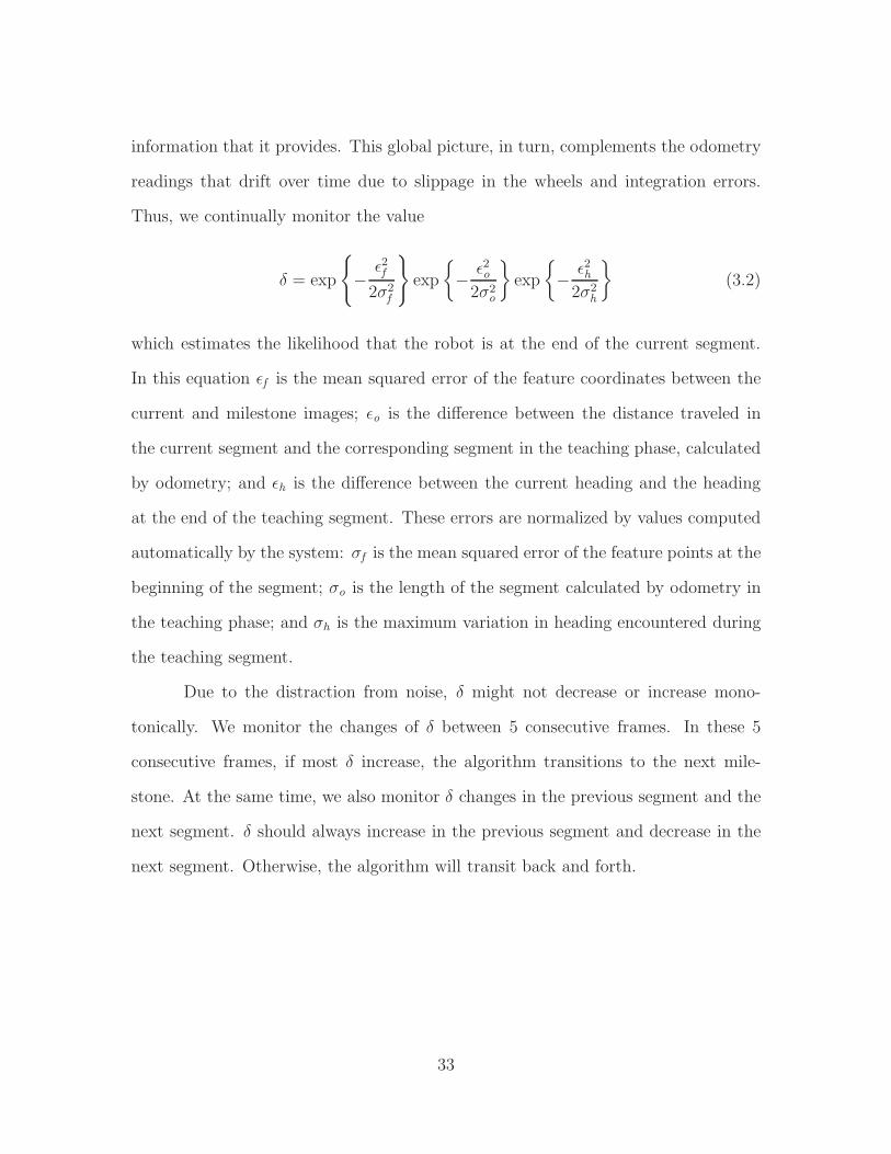
Turn left Turn right
Figure 3.9: Feature decision process. Top: Two milestone images from the indoorexperiment, with all the feature points overlaid. Bottom: Two current imageswithin each segment, as the robot moves toward the corresponding milestone location,with feature points overlaid. The features outlined by a rectangle (green in theelectronic version of the paper) are the ones for which one of the constraints is violated.In the left column, the features on the left half of the current image tell the robot toturn left. In the right column, the features on the right half of the current image tellthe robot to turn right.
Difficulty is encountered primarily when the robot has to turn near the corner of a
hallway containing no additional objects.
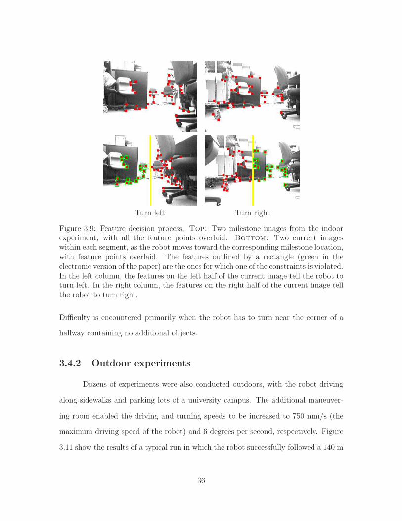
3.4.2 Outdoor experiments
Dozens of experiments were also conducted outdoors, with the robot driving
along sidewalks and parking lots of a university campus. The additional maneuver-
ing room enabled the driving and turning speeds to be increased to 750 mm/s (the
maximum driving speed of the robot) and 6 degrees per second, respectively. Figure
3.11 show the results of a typical run in which the robot successfully followed a 140 m
36

1 2 3 4 5 6 7 8−0.5
0
0.5
1
1.5
Frame
γ OK
Turn left
Turn right
1 2 3 4 5−2
0
2
4
6
8
Frame
γ Turn right
Turn left
OK
1 2 3 4 5−10
−8
−6
−4
−2
0
2
4
Frame
γ
Turn right
Turn left
OK
−100 −50 50 100
uD
−100
−80
−40
−20
20
40
80
100 uC
Turn right
OK
OKTurn left
−100 −80 −60 −40 −20 20 40 60 80 100
ut
−100 −80 −60 −40 −20 20 40 60 80 100
uD
−100
−80
−40
−20
20
40
80
100 uC
Turn right
Turn leftOK
OK−100 −80 −60 −40 −20 20 40 60 80 100
uD
−100
−80
−40
−20
20
40
80
100 uC
OK
Turn right
Turn leftOK
(a) Do not turn (b) Turn right (c) Turn left
Figure 3.10: Features vs. direction. Top: The normalized feature coordinates of allthe features plotted versus the image frame number for three segments of the indoorexperiment. Features below 0 vote for “turn left”, while those above 1 vote for “turnright”. Bottom: A snapshot of the features from frame 2 of each segment plotted onthe qualitative control decision space to show the instantaneous decision. The threesegments correspond to the points a, b, and c from Figure 3.8.
loop trajectory in a parking lot. The error was less than 1 m for two-thirds of the
sequence and remained below 3.5 m for the entire sequence.
0 50 100
−40
−20
0
20
40
60
x(m)
y(m
) teachingreplaystart
end
0 100 200 300 400 500 600 7000
1
2
3
4
time(s)
erro
r(m
)
Figure 3.11: Outdoor navigation. Top: The teaching and replay paths of the robotin an outdoor environment (parking lot). Bottom: Error versus distance traveled.
Figure 3.12 shows sample images from two experiments demonstrating the
37

robustness of the algorithm. In the first, the robot navigated a slanted ramp in a
40 m run, thus verifying that the algorithm does not require a flat ground plane. In
the second, the robot navigated a narrow road for 80 m while a pedestrian walked by
the robot and later a van drove by it. Because the milestone images change frequently,
the algorithm quickly recovered from the loss of features due to the occlusion caused
by the dynamic objects.
When a dynamic object (e.g., a person walking) comes into the view of the
robot, feature points on the background may be lost due to occlusion. Because the
algorithm treats all the features equally and because a new milestone image (defined
below) is taken frequently, this loss does not affect the performance of the algorithm
in practice as long as the occlusion is fairly small (say, one-fourth of the image). If the
occluding object is so large in the field of view that it causes a large number of feature
points to be lost, then there is not enough information for the algorithm to continue.
This problem can be solved by detecting the sudden loss of a large percentage of the
features and commanding the robot to stop until it is able to reacquire the features
once the object leaves the field of view.
A challenge of outdoor environments is the drastic change in illumination,
which is caused primarily by either (1) changing environmental conditions over time,
or (2) the automatic gain control of the camera adjusting to the difference between
shadow and sunlight. Figure 3.13 shows the importance of the lighting-insensitive
modification to the KLT feature tracking algorithm using two experiments. In the
first, there was significant change in the environmental lighting between the teaching
and replay phases due to changing cloud cover. In the second, the automatic gain
control of the camera caused the overall brightness of the scene to change significantly
because the robot moved from bright sunlight into a shadow. In both cases the original
KLT algorithm lost nearly all the features while the modified algorithm successfully
38

frame 1 frame 59 frame 240 frame 322
frame 255 frame 265 frame 663 frame 684
Figure 3.12: Running on the ramp with dynamic objects. Sample image frames fromtwo different sequences, one in which the robot traveled down and up a ramp (top),and the other containing dynamic objects (bottom). The circles indicate the features.
tracked many of them.
original modified original modified— Environmental changes — — Automatic gain control —
Figure 3.13: Results under changing lighting conditions. Left columns: Twoimages with features tracked using the original and modified KLT algorithms, withthe sun being occluded by clouds. Right columns: Two images from a sequencein which the automatic gain control caused a brightening of the image as the robotmoved from sun to shade.
39

3.4.3 Different cameras
Figure 3.14 shows the results of the approach using cameras with severe lens
distortion. In one experiment we used a wide-angle camera with a 3.5 mm focal
length and 110-degree field of view. The other experiment utilized an omnidirectional
camera with a 360-degree field of view. For both experiments we used the same
parameters as the previous experiments. The only change made to the code was to
discard the bottom half of the omnidirectional donut image. This step was necessary
because features behind the robot (whether viewed by an omnidirectional or standard
camera) move in a way that violates the fundamental assumptions of our approach.
In contrast, features in front of the camera obey the funnel constraints sufficiently
to be of use in keeping the robot on the path, despite their moving in curved image
paths due to the severe lens and catadioptric distortion. The average error of the
two experiments was 0.04 m and 0.04 m, respectively, while the maximum error was
0.13 m and 0.09 m.
0 1 2 3 4 5
0
1
2
3
4
x(m)
y(m
) TeachingReplay
start
end
0 1 2 3 4 5 6−1
0
1
2
3
4
x(m)
y(m
) TeachingReplay
startstart
end
Figure 3.14: Using cameras with severe lens distortion. The approach successfullyfollowing a path using a wide-angle camera (left) and an omnidirectional camera(right).
To further illustrate the lack of calibration, we conducted an outdoor exper-
iment in which the robot navigated the same 50 m path twice. In the first run the
40

robot used the Logitech Quickcam Pro 4000 camera, while in the second run it used
an Imaging Source DFK21F04 Firewire camera with an 8.0 mm F1.2 lens. The same
camera was used for both teaching and replay. As shown in Figure 3.15, the algorithm
was able to successfully follow the path using either camera, without changing any
parameters between runs.
0 5 10 15−40
−30
−20
−10
0
x(m)
y(m
)
TeachingReplay
start
end
0 5 10 15−40
−30
−20
−10
0
x(m)
y(m
)TeachingReplay
start
end
Figure 3.15: Using two different uncalibrated cameras. Teaching and replay paths forthe robot using two different uncalibrated cameras, with the same system parameters.Left: Logitech QuickCam Pro 4000 USB webcam, Right: Imaging Source DFK21F04 Firewire camera.
Three additional experiments are shown in Figure 3.16. In the first, a scout
robot was sent along an outdoor path. Another robot, which received the trans-
mitted path information, was then able to follow the same path as the scout. This
demonstrates a natural application to swarm robotics, where calibrating dozens or
hundreds of cameras would be prohibitive, especially if recalibration is needed when-
ever the lenses are refocused or the cameras adjusted. The second experiment shows
the robot following a path along rough terrain, in which roll and tilt angles up to 5
degrees were encountered. The roll angle compensation described earlier was suffi-
cient to enable the robot to remain on the path. In the third, a path with several
sharp turns is demonstrated. This ability is achieved by setting the replay driving
speed to be that of the teaching driving speed, which is decreased during a turn.
41

−20 −10 0 10 20 30 40 50−50
−40
−30
−20
−10
0
x(m)
y(m
)
scout robotfollowing Robot
start
end
0 20 40 60
−50
−40
−30
−20
−10
0
x (m)
y (m
)
teachingreplay
start
end
0 5 10 15 20 25 30 35−5
0
5
10
15
20
x(m)
y(m
)
TeachingReplaystart
end
Figure 3.16: Applications for scout robot. Left: The robot followed a path takenearlier by a scout robot. Middle: A path on rough terrain. Right: A path withsharp turns.
3.4.4 Repeatability and accuracy
Additionally, the algorithm was tested in various scenarios to quantitatively
measure its accuracy and repeatability. Table 3.1 displays the results of the algorithm
compared with those of our earlier version [23] which did not use odometry, relied upon
a bang-bang control scheme, and did not compensate for the camera roll angle. The
algorithms were tested in three environments: a 15 m path in an indoor laboratory
environment with rich texture for feature tracking, a 60 m trajectory in an outdoor
paved parking lot, and a 40 m path along unpaved terrain. In each case, we conducted
ten trials and recorded the final 2D location of the robot for each trial: {xi}ni=1, where
xi ∈ R2 and n = 10. Accuracy was measured as the RMS Euclidean distance to the
final ground truth location:√
1n
∑n
i=1 || xi − xgt ||2. Repeatability was measured
as the standard deviation of the final locations:√
1n
∑n
i=1 || xi − µ ||2, where µ =
1n
∑n
i=1 xi . While the earlier algorithm works well when the ground is paved and the
scenery is rich in texture, the improved algorithm is more robust, achieving maximum
errors of only 0.23 m, 1.20 m, and 1.76 m, respectively, compared with 0.45 m, 1.20 m,
and 5.68 m for the earlier algorithm.
The algorithm assumes that the robot is placed in the same initial location
in both the teaching and replay phases. To test the sensitivity to this assumption,
42
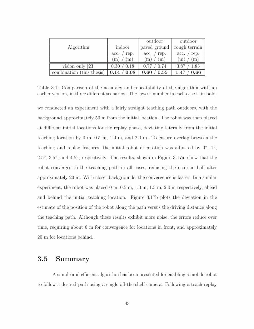
outdoor outdoorAlgorithm indoor paved ground rough terrain
acc. / rep. acc. / rep. acc. / rep.(m) / (m) (m) / (m) (m) / (m)
vision only [23] 0.30 / 0.18 0.77 / 0.74 3.87 / 1.85combination (this thesis) 0.14 / 0.08 0.60 / 0.55 1.47 / 0.66
Table 3.1: Comparison of the accuracy and repeatability of the algorithm with anearlier version, in three different scenarios. The lowest number in each case is in bold.
we conducted an experiment with a fairly straight teaching path outdoors, with the
background approximately 50 m from the initial location. The robot was then placed
at different initial locations for the replay phase, deviating laterally from the initial
teaching location by 0 m, 0.5 m, 1.0 m, and 2.0 m. To ensure overlap between the
teaching and replay features, the initial robot orientation was adjusted by 0o, 1o ,
2.5o, 3.5o, and 4.5o , respectively. The results, shown in Figure 3.17a, show that the
robot converges to the teaching path in all cases, reducing the error in half after
approximately 20 m. With closer backgrounds, the convergence is faster. In a similar
experiment, the robot was placed 0 m, 0.5 m, 1.0 m, 1.5 m, 2.0 m respectively, ahead
and behind the initial teaching location. Figure 3.17b plots the deviation in the
estimate of the position of the robot along the path versus the driving distance along
the teaching path. Although these results exhibit more noise, the errors reduce over
time, requiring about 6 m for convergence for locations in front, and approximately
20 m for locations behind.
3.5 Summary
A simple and efficient algorithm has been presented for enabling a mobile robot
to follow a desired path using a single off-the-shelf camera. Following a teach-replay
43
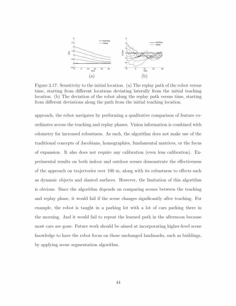
0 5 10 15 20 25−0.5
0
0.5
1
1.5
2
2.5
3
x(m)y(
m)
teachingreplaydata3data4data5data6
0 5 10 15 20−3
−2
−1
0
1
2
3
x(m)
∆ x(
m)
teachingreplay
(a) (b)
Figure 3.17: Sensitivity to the initial location. (a) The replay path of the robot versustime, starting from different locations deviating laterally from the initial teachinglocation. (b) The deviation of the robot along the replay path versus time, startingfrom different deviations along the path from the initial teaching location.
approach, the robot navigates by performing a qualitative comparison of feature co-
ordinates across the teaching and replay phases. Vision information is combined with
odometry for increased robustness. As such, the algorithm does not make use of the
traditional concepts of Jacobians, homographies, fundamental matrices, or the focus
of expansion. It also does not require any calibration (even lens calibration). Ex-
perimental results on both indoor and outdoor scenes demonstrate the effectiveness
of the approach on trajectories over 100 m, along with its robustness to effects such
as dynamic objects and slanted surfaces. However, the limitation of this algorithm
is obvious. Since the algorithm depends on comparing scenes between the teaching
and replay phase, it would fail if the scene changes significantly after teaching. For
example, the robot is taught in a parking lot with a lot of cars parking there in
the morning. And it would fail to repeat the learned path in the afternoon because
most cars are gone. Future work should be aimed at incorporating higher-level scene
knowledge to have the robot focus on those unchanged landmarks, such as buildings,
by applying scene segmentation algorithm.
44

Chapter 4
Person Following
Visual person following with a mobile robot is another important research
topics in machine vision and robotics. New and innovative techniques are constantly
being developed. However, despite the impressive results obtained, it is clear that
no approach can perform reliably in all situations. People are non-rigid objects and
are difficult to model geometrically; plus, the occlusions and distractions from the
environment, including other people, can confuse the tracker. And the foreground
segmentation is more difficult from a moving platform than from a fixed viewpoint
because the background undergoes motion relative to the platform, and therefore the
static background subtraction is not applicable. To keep up with a walking person
in real-time, detection and tracking algorithm must be fast enough and require very
quick focus of attention. The most popular approach utilizes appearance properties,
such as color, that distinguish the target person from the surrounding environment.
This method requires the person wear clothes that have a different color from the
background. In addition, lighting changes tend to cause serious problems for color-
based techniques. Other researchers have applied optic flow to the problem. These
techniques are subject to drift as the person moves about the environment, particu-
45
larly with out-of-plane rotation, and are therefore limited to short paths.
This chapter presents a approach for a person following vision system that
addresses these issues by fulfilling the following criteria:
• allowing person wearing the same color as the background.
• allowing person rotating arbitrarily during tracking.
• allowing person walking in a cluttered environment including other people walk-
ing around.
Firstly the overall architecture of the system is described in Section 4.1. Sec-
tion 4.2 describes the sparse disparity map constructed by feature matching between
two stereo images. Section 4.3 demonstrates the detailed algorithm to extract per-
son from background. Section 4.4 presents the robot control strategy. Experimental
results are shown in Section 4.5. Section 4.6 closes with a summary.
4.1 System overview
The system consists of a pair of forward-facing stereo cameras on a mobile
robot. The Binocular Sparse Feature Segmentation (BSFS) for processing the binoc-
ular video, shown in Figure 4.1, consists of two modes. In detection mode, sparse
features are matched between the two images to yield disparities, from which the
segmentation of foreground and background is performed. Once the person is de-
tected the system enters tracking mode, in which the existing features on the person
are tracked from frame to frame. Features not deemed to belong to the person are
discarded, and once the person has been lost the system returns to detection mode.
In both modes the results of the feature algorithm are combined with the output of
46

Figure 4.1: Overview of the person following algorithm.
a face detector, which provides additional robustness when the person is facing the
camera.
4.2 Computing disparity between feature points
Feature points are automatically matched, both between the two stereo images
and in one sequence over time, using the Lucas-Kanade approach [7, 84, 95]. In
detection mode, the features are matched between the stereo images to compute the
disparity between them. At time t , features are selected in the left image I Lt and
matched in the right image I Rt , after which the resulting features in the right image
are matched again in the left image. This left-right consistency check [35] discards
features whose initial and final locations are not within a tolerance ǫt , thus improving
robustness by removing unreliable features. (We set ǫt = 2 in our experiments.) The
horizontal disparities of the remaining features are stored for the later processing
stages. (Since the cameras are approximately aligned, the vertical disparities are
nearly zero and are therefore ignored.) The result on a pair of images is shown in
47
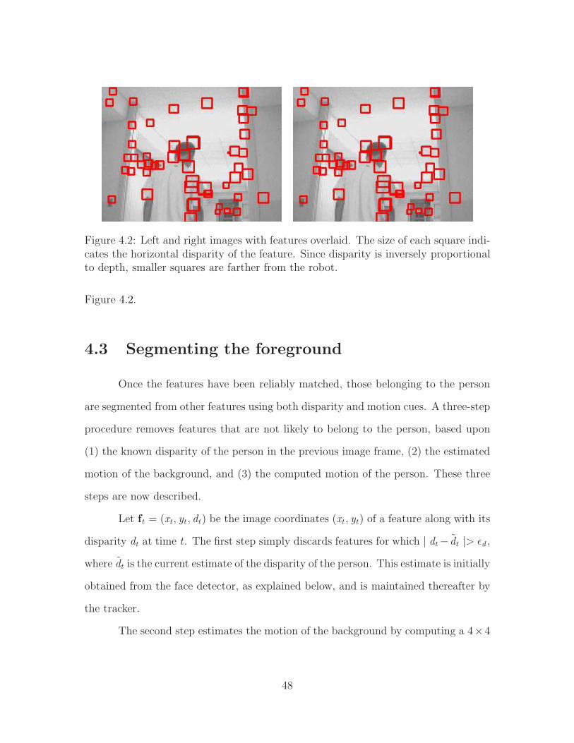
Figure 4.2: Left and right images with features overlaid. The size of each square indi-cates the horizontal disparity of the feature. Since disparity is inversely proportionalto depth, smaller squares are farther from the robot.
Figure 4.2.
4.3 Segmenting the foreground
Once the features have been reliably matched, those belonging to the person
are segmented from other features using both disparity and motion cues. A three-step
procedure removes features that are not likely to belong to the person, based upon
(1) the known disparity of the person in the previous image frame, (2) the estimated
motion of the background, and (3) the computed motion of the person. These three
steps are now described.
Let ft = (xt , yt , dt) be the image coordinates (xt , yt) of a feature along with its
disparity dt at time t . The first step simply discards features for which | dt− dt |> ǫd ,
where dt is the current estimate of the disparity of the person. This estimate is initially
obtained from the face detector, as explained below, and is maintained thereafter by
the tracker.
The second step estimates the motion of the background by computing a 4×4
48
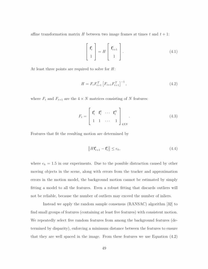
affine transformation matrix H between two image frames at times t and t + 1:
fit
1
= H
fit+1
1
. (4.1)
At least three points are required to solve for H :
H = FtFTt+1
[Ft+1F
Tt+1
]−1, (4.2)
where Ft and Ft+1 are the 4×N matrices consisting of N features:
Ft =
f1t f2t · · · fNt
1 1 · · · 1
4XN
. (4.3)
Features that fit the resulting motion are determined by
∥∥H fit+1 − fit∥∥ ≤ ǫh , (4.4)
where ǫh = 1.5 in our experiments. Due to the possible distraction caused by other
moving objects in the scene, along with errors from the tracker and approximation
errors in the motion model, the background motion cannot be estimated by simply
fitting a model to all the features. Even a robust fitting that discards outliers will
not be reliable, because the number of outliers may exceed the number of inliers.
Instead we apply the random sample consensus (RANSAC) algorithm [32] to
find small groups of features (containing at least five features) with consistent motion.
We repeatedly select five random features from among the background features (de-
termined by disparity), enforcing a minimum distance between the features to ensure
that they are well spaced in the image. From these features we use Equation (4.2)
49

to calculate the background motion Hb , which is then applied to all the background
features to record the number of inliers. This process is repeated several times, and
the motion model with the largest number of inliers is taken to be the background
motion. Once the background motion has been estimated, the foreground features
that do not match this motion model are discarded using Equation (4.4).
To remove independently moving objects, the third step calculates the motion
model Hp of the person using the remaining features. RANSAC is applied, as be-
fore, to yield the dominant motion among these features. A second motion model is
then determined by applying RANSAC to the features that do not fit the dominant
motion model. Two cues are used to distinguish the person from another moving
object, namely the size of the group and the proximity to the previous position of
the person. Thus, the group that maximizes n(si) − m(si), i = 1, 2, where m(si) is
the mean squared error Mi between the centroid of the ith group and the previous
person position, taken in the horizontal direction: m(si) = Mi/(M1 + M2); and n(si)
is the relative number of features Ni of the ith group: n(si) = Ni/(N1 + N2). The
remaining features are then projected onto the horizontal axis, and the largest con-
nected component is retained. The bottom right image of Figure 4.3 shows the final
result of the detector.
After these steps, the features that remain are assumed to belong to the person.
If the number of features exceeds a threshold, then the person is detected, and the
system enters tracking mode. An example of the three steps applied to a portion of
the video sequence is shown in Figure 4.3. The person is typically detected after just
two image frames.
An example showing the results of the algorithm when the background has
a similar disparity as the person is shown in Figure 4.4. In this case the disparity
test (Step 1) finds almost no features on the background, thus rendering the first two
50
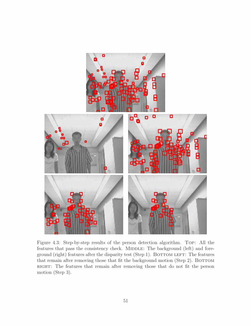
Figure 4.3: Step-by-step results of the person detection algorithm. Top: All thefeatures that pass the consistency check. Middle: The background (left) and fore-ground (right) features after the disparity test (Step 1). Bottom left: The featuresthat remain after removing those that fit the background motion (Step 2). Bottom
right: The features that remain after removing those that do not fit the personmotion (Step 3).
51

steps ineffective at discarding background features. Step 3, however, uses the motion
of the person to correctly discard the features on the background, resulting in features
that lie almost entirely on the person. Figure 4.4 shows that the algorithm does not
assume that the person is the closest object. As shown in Figure 4.5, this procedure is
insufficient when the person is not moving, because Step 2 of the algorithm incorrectly
discards the features on the person due to the similarity between the motion of the
person and background. To solve this problem, the robot simply waits until a sufficient
number of features are detected before moving.
In both the detection and tracking modules, the Viola-Jones frontal face de-
tector [98] is applied at constant intervals. The face detector uses integral images
to compute features resembling Haar wavelets, and a cascade architecture is used to
enable the algorithm to efficiently evaluate all image locations. This detector is used
both to initialize the system and to enhance robustness when the person is facing the
camera. In both modes, the face detector is combined with the results of the detection
or tracking algorithms by discarding features that lie outside a body bounding box
just below the face detection. Note, however, that our system does not require the
person to face the camera.
4.4 Tracking and camera control
Once the person has been detected, control passes to the tracking module. The
person is tracked using the same features by applying Lucas-Kanade from frame to
frame. Over time features are lost due to several reasons. Some features are discarded
automatically by the Lucas-Kanade algorithm because a sufficient match is not found
in the next frame. More commonly, features drift from the person to the background,
in particular when the person self-occludes by rotating. To detect this event, features
52
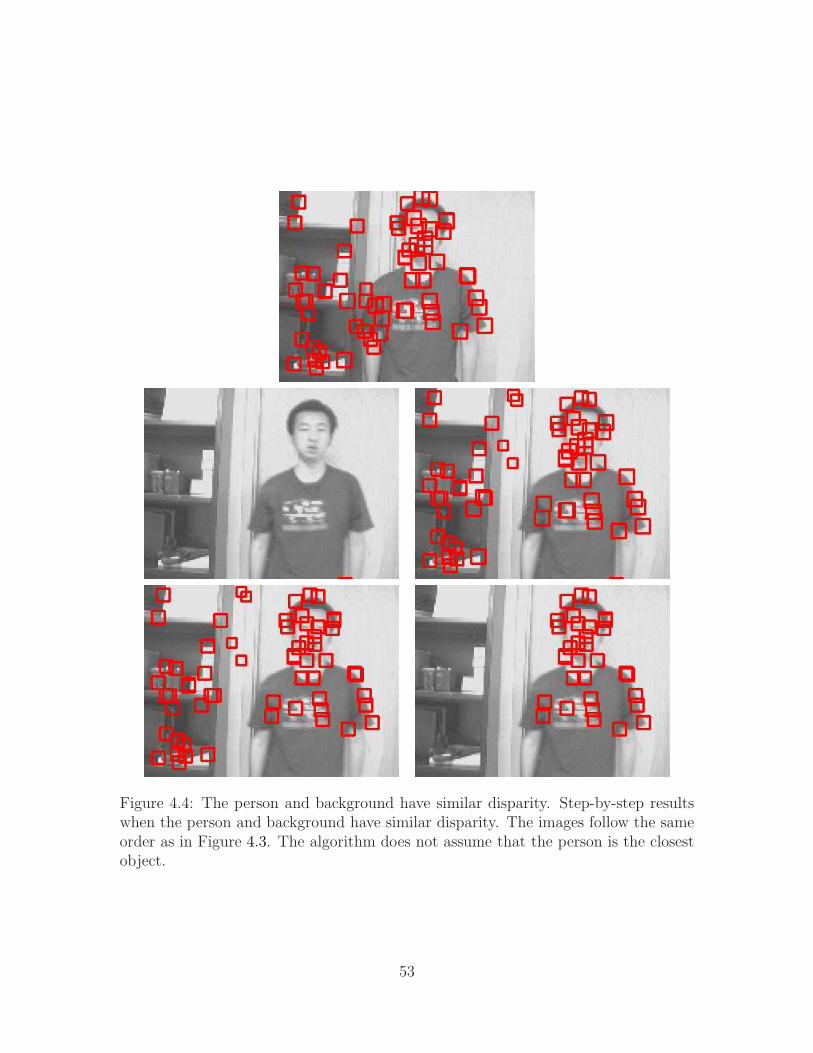
Figure 4.4: The person and background have similar disparity. Step-by-step resultswhen the person and background have similar disparity. The images follow the sameorder as in Figure 4.3. The algorithm does not assume that the person is the closestobject.
53

Figure 4.5: Two additional examples. Top: All the features that pass the consistencycheck. Bottom: The final result of the person detection algorithm when the personis still (left) and moving (right).
54
are discarded when their disparity differs from the disparity of the person by more
than the threshold ǫd . When a significant number of the original features have been
lost, the tracker gives up, and control returns to the detection module.
A simple proportional control scheme is applied to the robot motors, i.e., the
driving speed σd is set to be proportional to the inverse of the disparity d to the
person, while the turning speed σt is set to be proportional to the product of the
horizontal position p of the person in the image relative to center and the disparity,
as follows:
σd = K1d , σt = K2pd , (4.5)
where K1, K2 are constants (80 and 0.01, respectively). We have found this simple
control scheme to be sufficient for our purposes.
4.5 Experimental results
The proposed algorithm was implemented in Visual C++ on a Dell Insp-
iron 700m laptop (1.6 GHz) controlling an ActivMedia Pioneer P3-AT mobile robot.
Mounted on a tripod on the robot were two ImagingSource DFK21F04 Firewire cam-
eras with 8.0 mm F1.2 lenses spacing approximately 5.5 cm apart yielding images of
size 320 × 240. The OpenCV library [1] was used for the feature detection, feature
tracking, and face detection. The maximum driving speed of the robot was 0.75 me-
ters per second, while the maximum turning speed was 30 degrees per second. The
entire system operates at an average of 16 Hz.
The algorithm has been tested extensively in indoor environments and moder-
ately in outdoor environments. Figure 4.6 shows a typical run of the system, with the
robot traveling over 100 meters. To initialize, the person faced the robot, after which
55

the person walked freely at approximately 0.8 m/s, sometimes facing the robot and
other times turning away. The environment was challenging because it contained a
textured background, other people walking around, some lighting changes, and image
saturation due to a bright ceiling light. Some example images from two experiments
are shown in Figure 4.7 to demonstrate the ability of the system to handle an untex-
tured shirt that is the same color as the background, as well as moving objects in the
scene.
To further test the robustness of the algorithm, five people were asked to walk
around the environment in a serpentine path for approximately five minutes. Two
experiments were captured for each person, one at a speed of approximately 0.5 m/s
and another at approximately 0.8 m/s. The shirts of the people were white, white,
yellow, blue, and textured. Some of the people always faced the robot, some rarely
faced the robot, and other faced the robot occasionally. Of the ten trials, the robot
succeeded nine times (90% success rate). The only failure was caused by the person
walking quickly away from the camera with an untextured shirt. In other experiments,
the robot has successfully tracked the person for more than 20 minutes without an
error.
We compared our algorithm with a popular color histogram-based algorithm,
namely the Camshift technique in OpenCV. The latter was found to be much more
likely to be distracted by background or lighting changes than ours. Figure 4.8 shows
a typical run, in which the robot lost the person when he turned around the corner,
whereas our algorithm successively followed the person to the end. In this experiment
the person intentionally walked in a fairly straight path, and the person wore a shirt
whose color was distinct from the background, in order to make the task easier for
the color-based algorithm. Some images from a different experiment comparing the
two algorithms are shown in Figure 4.9. It should be noted that more advanced color-
56

Figure 4.6: Path of a person following experiment. The robot path as it followed theperson through the hallways of our laboratory in an experiment.
based tracking algorithms will also fail whenever the target has a similar appearance
to the background.
4.6 Summary
We have presented an algorithm for following a person using a grayscale stereo
pair of cameras on a mobile robot using sparse features. The features are matched
between the stereo images and then tracked over time, while a RANSAC-based pro-
cedure discards features that do not belong to the person. An efficient face detector is
used both to initialize the system and to increase robustness when the person is facing
the camera. Compared with previous techniques, this approach has the advantage of
not requiring the user to wear a shirt colored distinctly from the background or to
always face the robot. It also demonstrates some amount of insensitivity to lighting
variations and moving people in the scene.
57
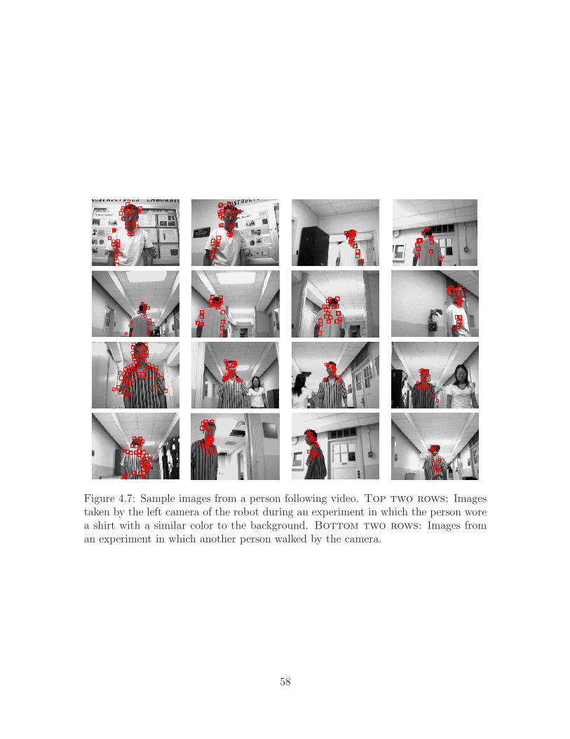
Figure 4.7: Sample images from a person following video. Top two rows: Imagestaken by the left camera of the robot during an experiment in which the person worea shirt with a similar color to the background. Bottom two rows: Images froman experiment in which another person walked by the camera.
58

Figure 4.8: Comparison with color-histogram-based tracking. The color-based al-gorithm lost the person when he turned down the hallway, whereas our algorithmsucceeded.
Figure 4.9: Sample images for comparison with color-histogram-based tracking. Theresults of the color-based algorithm (top) and our algorithm (bottom) in an envi-ronment with a textured background. The former loses the person, while the lattersucceeds.
59
Chapter 5
Door Detection
Doors are important landmarks for indoor mobile robot navigation. They mark
the entrance/exit of rooms in many offices and laboratory environments. The ability
of a robot to detect doors can be a key point for a robust navigation. What visual
characteristics make a door appear to be a door. In other word, what features can be
used by computer vision to automatically locate doors in images? Figure 5.1 shows
the main features which characterize a door. However, these features are not always
present or cannot always be detected in a single camera image, for example, the color
of door and wall might not be different; the kick plate might not exist; the top frame
of the door (lintel) might be occluded; the door knob and hinge might be too small in
the image to be detected. It is our belief that the solution to this problem cannot be
achieved by focusing only upon one piece of local evidence. Rather, the integration
of a variety of cues is needed to overcome the noise of sparse, local measurements. As
a result, we approach the problem recognizing that recognition is inherently a global
process.
As shown in Figure 5.2, two vision-based door detection algorithms are devel-
oped, one based on Adaboost and the other on Data-Driven Markov Chain Monte
60
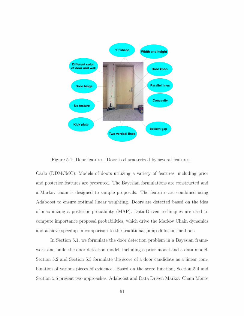
Figure 5.1: Door features. Door is characterized by several features.
Carlo (DDMCMC). Models of doors utilizing a variety of features, including prior
and posterior features are presented. The Bayesian formulations are constructed and
a Markov chain is designed to sample proposals. The features are combined using
Adaboost to ensure optimal linear weighting. Doors are detected based on the idea
of maximizing a posterior probability (MAP). Data-Driven techniques are used to
compute importance proposal probabilities, which drive the Markov Chain dynamics
and achieve speedup in comparison to the traditional jump diffusion methods.
In Section 5.1, we formulate the door detection problem in a Bayesian frame-
work and build the door detection model, including a prior model and a data model.
Section 5.2 and Section 5.3 formulate the score of a door candidate as a linear com-
bination of various pieces of evidence. Based on the score function, Section 5.4 and
Section 5.5 present two approaches, Adaboost and Data Driven Markov Chain Monte
61

Figure 5.2: Overview of our approach to detect doors. Several features are combinedusing the AdaBoost or DDMCMC
Carlo (DDMCMC), to detect doors. In Section 5.6 we propose three methods to au-
tomatically detect wall/door color. Section 5.7 proposes an approach to detect open
doors. In addition to door detection, we develop a door tracking algorithm, which
is presented in Section 5.8. Experimental results are shown in Section 5.9. Finally,
Section 5.10 presents the conclusions.
5.1 Bayesian formulation
In this section, we formulate the problem in a Bayesian framework. Assuming
that the camera is oriented so that the image plane is perpendicular to the floor, a
door d = (xl , xr , ylt , ylb , yrt , yrb) in an image I is represented using the six coordinates
62

of the four end points of two vertical line segments ℓl and ℓr . Our goal is to find
the number of doors in the image, along with the location of each door. Invoking
the first-order Markov assumption, and letting d1, . . . ,dk to represent the sequence
of k doors from left to right in the image, the goal is expressed probabilistically as
maximizing
p(k ,d1, . . . ,dk | I ) = p(d1 | I )p(k | I )k∏
i=2
p(di | I ,di−1). (5.1)
A straightforward approach to solve this problem would be to apply reversible
jump Markov chain Monte Carlo (RJMCMC) to simultaneously estimate the number
k and the joint configuration of all the doors. Such an approach, however, is noto-
riously computationally intensive. In contrast, the formulation above suggests that
a simpler approach might be sufficient: search the image from left to right (or vice
versa) in a sequential manner to find the doors one at a time. Since the coupling be-
tween the doors can be modeled as a prior on location, the primary problem becomes
to find a single door given the image by maximizing p(d | I ), which, according to
Bayes’ rule, is
p(d | I ) ∝ p(I | d)p(d). (5.2)
Taking the log likelihood, this is equivalent to maximizing the following functional:
E (d) = Ψdata(I | d) + Ψprior (d), (5.3)
where the likelihood is p(I | d) = exp{Ψdata(I | d)}, and the prior is p(d) =
exp{Ψprior (d)}.
63

5.2 Prior model
The prior model captures information about the expected door configuration
without considering image evidence relevant to the particular door being found. We
formulate the prior score of a door candidate as a linear combination of various pieces
of evidence:
Ψprior (d) =
Nprior∑
i=1
αi fi(d), (5.4)
where Nprior is the number of tests aggregated, and αi is the weight that governs the
relative importance of the ith test. (As described later, the Adaboost algorithm will
be used to ensure optimal weighting.) All the tests fi are normalized to yield values
between 0 and 1, leading to a formulation of expert opinions similar to the sum rule
of Kittler and colleagues [49, 48, 92].
Our approach employs two tests (Nprior = 2). First, we compare the width w
of the door in world coordinates with the expected width w of real doors:
f1(d) = exp
{−(w − w)2
2σ2w
}. (5.5)
Several real world doors were measured in order to determine the expected door width
and standard deviation, leading to w = 0.96 m, and σw = 0.08 m. To enable the
measuring of the door width in world coordinates, the camera is first calibrated by
capturing an image of a piece of paper of known dimensions placed on the floor. The
normalized Direct Linear Transformation (DLT) [41] is used to calculate a homogra-
phy between the floor plane and the image plane, which enables the image to world
transformation of the two points at the bottom of the door.
Secondly, we expect the height of the two vertical door edges (in world coordi-
64
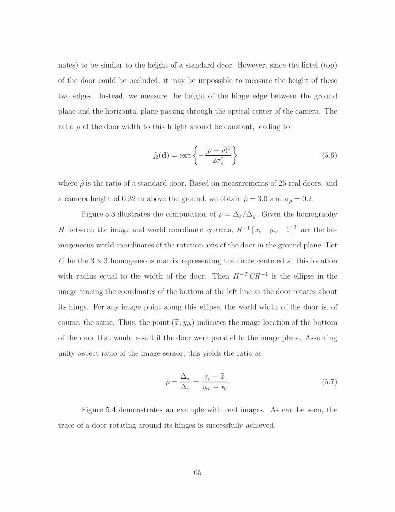
nates) to be similar to the height of a standard door. However, since the lintel (top)
of the door could be occluded, it may be impossible to measure the height of these
two edges. Instead, we measure the height of the hinge edge between the ground
plane and the horizontal plane passing through the optical center of the camera. The
ratio ρ of the door width to this height should be constant, leading to
f2(d) = exp
{−(ρ− ρ)2
2σ2ρ
}, (5.6)
where ρ is the ratio of a standard door. Based on measurements of 25 real doors, and
a camera height of 0.32 m above the ground, we obtain ρ = 3.0 and σρ = 0.2.
Figure 5.3 illustrates the computation of ρ = ∆x/∆y . Given the homography
H between the image and world coordinate systems, H−1 [ xr yrb 1 ]T are the ho-
mogeneous world coordinates of the rotation axis of the door in the ground plane. Let
C be the 3× 3 homogeneous matrix representing the circle centered at this location
with radius equal to the width of the door. Then H−TCH−1 is the ellipse in the
image tracing the coordinates of the bottom of the left line as the door rotates about
its hinge. For any image point along this ellipse, the world width of the door is, of
course, the same. Thus, the point (x , yrb) indicates the image location of the bottom
of the door that would result if the door were parallel to the image plane. Assuming
unity aspect ratio of the image sensor, this yields the ratio as
ρ =∆x
∆y
=xr − x
yrb − v0
. (5.7)
Figure 5.4 demonstrates an example with real images. As can be seen, the
trace of a door rotating around its hinges is successfully achieved.
65
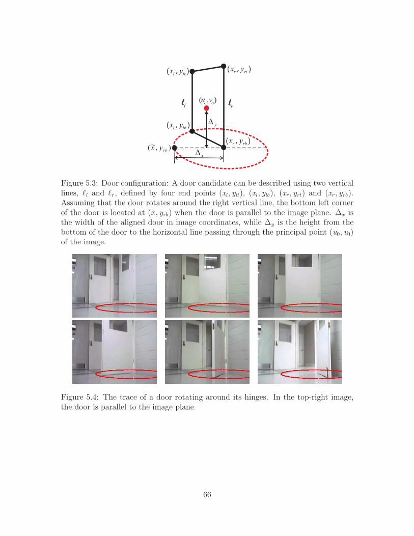
( , )l lt
x y
( , )l lb
x y
( , )r rt
x y
( , )r rb
x y),~( rbyx
y?
x?
),( oo vull rl
Figure 5.3: Door configuration: A door candidate can be described using two verticallines, ℓl and ℓr , defined by four end points (xl , ylt), (xl , ylb), (xr , yrt) and (xr , yrb).Assuming that the door rotates around the right vertical line, the bottom left cornerof the door is located at (x , yrb) when the door is parallel to the image plane. ∆x isthe width of the aligned door in image coordinates, while ∆y is the height from thebottom of the door to the horizontal line passing through the principal point (u0, v0)of the image.
Figure 5.4: The trace of a door rotating around its hinges. In the top-right image,the door is parallel to the image plane.
66

5.3 Data model
Similar to the prior model, the data model is formulated as a linear combina-
tion of evidences:
Ψdata(I | d) =
Ndata∑
j=1
βjgj (I | d), (5.8)
where the weights βj are chosen based on Adaboost, and all the tests gj are normalized
between 0 and 1. We now describe the Ndata = 9 tests.
5.3.1 Image gradient along edges (g1)
Perhaps the most distinguishing visual characteristic of doors in images is the
change in intensity that usually accompanies the sides of the door. As a result, we
measure
g1(d, I ) = exp
{−∑
x∈Re
∣∣∣(∇I (x))T n(x)∣∣∣}
, (5.9)
where x is a pixel on the door edge, ∇I (x) is the 2D image gradient at the pixel, and
n(x) is the normal to the door edge at the pixel. The set Re of pixels includes the
left and right edges of the door, the bottom edge, and the top edge (if xlt 6= 0 and
xrt 6= 0). The gradient of the image is computed using a 3-tap separable Gaussian
derivative filter with a standard deviation of 1 pixel.
5.3.2 Placement of top and bottom edges (g2 and g3)
After computing the gradient of the image, vertical and horizontal line seg-
ments are found by applying the Douglas-Peucker line fitting algorithm [28], as modi-
fied in [24], to the output of the Canny edge detector. Appendix B presents the detail
67

of the modified Douglas-Peucker line fitting algorithm. The horizontal segments be-
tween the two vertical door edges are compared to determine the topmost segment,
which is then extended to intersect with the vertical edges, yielding expected values
ylt and yrt for the top points of the two edges. If there is no such segment, then
ylt = yrt = 0, indicating a lintel-occluded door. Similarly, the bottom endpoints of
the vertical edges are compared with the line forming the boundary between the wall
and the floor:
g2(I | d) = exp
{−(ylt − ylt)
2
2σ2t
− (yrt − yrt)2
2σ2t
}(5.10)
g3(I | d) = exp
{−(ylb − ylb)
2
2σ2b
− (yrb − yrb)2
2σ2b
}, (5.11)
where ylb and yrb are the intersection of the wall-floor boundary with the two vertical
edges, where the wall-floor boundary is computed by Image-based segmentation of
indoor corridor floors [58]. The standard deviations σt and σb are set to 5 pixels.
5.3.3 Color and texture (g4 and g5)
Color provides a helpful cue to distinguish the door from its surroundings. We
use the Bhattacharyya coefficient
g4(I | d) = 1−Ncol∑
i=1
√φ(i)φwall(i) (5.12)
to compare the normalized color histogram φ computed using the pixels inside the
door parallelogram, and the normalized color histogram φwall that models the colors
in the wall, where Ncol = 83 is the number of bins in the histogram. The HSV
(hue, saturation, value) color space is used due to its insensitivity to illumination
changes compared with RGB. In our system the robot builds a model of the wall
68

color automatically as it moves down the corridor, described later.
Although the top half of a door may contain windows, signs, or flyers, the
bottom half of a door is often untextured. We measure texture using the entropy of
the normalized histogram of the image gradient magnitude and phase:
g5(I | d) = 1− 1
η
Ntex∑
i=1
Mtex∑
j=1
φtex(i , j ) log (φtex(i , j )), (5.13)
where i and j index the magnitude and phase, respectively, in the histogram φtex ;
Ntex = 16 and Mtex = 8 are the number of bins along the two directions of the
histogram; and η = log (NtexMtex )−1 is the entropy of a uniform distribution, used to
normalize the result. Entropy is used to avoid being distracted by strong intensity
edges that may occur near the bottom of the door, due to the boundary of the kick
plate. Typically, such edges are fairly localized in magnitude and phase, thus resulting
in low entropy.
5.3.4 Kick plate (g6)
Figure 5.5: Kick plate. Left: A door with a kick plate. Right: The segmentationof the image using the method of Felzenszwalb et al. [31]. The kick plate is the olivegreen region at the bottom of the door.
Some doors have kick plates near the bottom which provide an additional cue
for door detection. The image is first segmented using the method of Felzenszwalb et
al. [31], as shown in Figure 5.5.
69
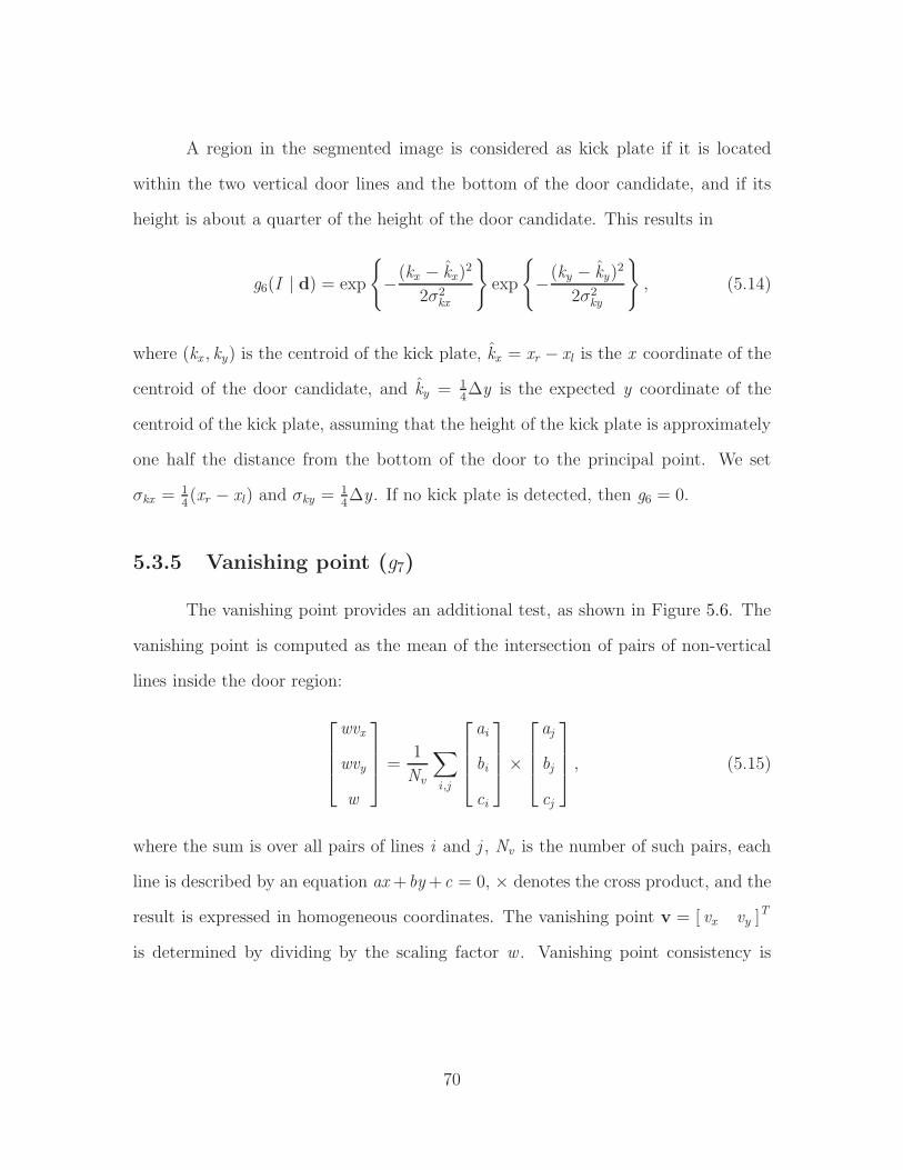
A region in the segmented image is considered as kick plate if it is located
within the two vertical door lines and the bottom of the door candidate, and if its
height is about a quarter of the height of the door candidate. This results in
g6(I | d) = exp
{−(kx − kx)
2
2σ2kx
}exp
{−(ky − ky)
2
2σ2ky
}, (5.14)
where (kx , ky) is the centroid of the kick plate, kx = xr − xl is the x coordinate of the
centroid of the door candidate, and ky = 14∆y is the expected y coordinate of the
centroid of the kick plate, assuming that the height of the kick plate is approximately
one half the distance from the bottom of the door to the principal point. We set
σkx = 14(xr − xl) and σky = 1
4∆y . If no kick plate is detected, then g6 = 0.
5.3.5 Vanishing point (g7)
The vanishing point provides an additional test, as shown in Figure 5.6. The
vanishing point is computed as the mean of the intersection of pairs of non-vertical
lines inside the door region:
wvx
wvy
w
=
1
Nv
∑
i ,j
ai
bi
ci
×
aj
bj
cj
, (5.15)
where the sum is over all pairs of lines i and j , Nv is the number of such pairs, each
line is described by an equation ax +by +c = 0, × denotes the cross product, and the
result is expressed in homogeneous coordinates. The vanishing point v = [ vx vy ]T
is determined by dividing by the scaling factor w . Vanishing point consistency is
70

measured by
g7(I | d) = exp
{−(vx − vx )
2
2σ2vx
}exp
{−(vy − vy)
2
2σ2vy
}, (5.16)
where v = [ vx vy ]T is the vanishing point estimated as the mean of the intersection
of pairs of non-vertical lines outside the door. We set σvx and σvy as 110
of the width
and height, respectively, of the image.
Figure 5.6: Vanishing point. Left: The bottom line of a door or wall/floor boundaryintersects the vanishing point. Right: In contrast, a distracting line caused byshadows does not.
5.3.6 Concavity (g8)
In many environments doors are receded into the wall, creating a concave
shape for the doorway. A simplified concave door structure is illustrated in Figure 5.7,
leading to two observations regarding the intensity edges:
• A slim “U” exists consisting of two vertical lines (the door edge and jamb) and
one horizontal line (between the door frame and floor); and
• The bottom edge of the door is slightly recessed from the wall-floor edge.
Let (x , y) be a pixel on the line formed by extending the wall/floor boundary
in front of the door (the dashed line in the figure), and let (x , yb) be the pixel on
71

the bottom of the door in the same column of the image. The slim “U” is tested by
comparing its width wu with an expected width wu :
hU = exp
{−(wu − wu)2
2σ2u
}, (5.17)
while the recession is tested by
hR = exp
{−(y − yb −∆yrec)
2
2σ2r
}, (5.18)
where wu = 14(xr − xl), ∆yrec = 2 pixels, σu = 2 pixels, and σr = 1
4(xr − xl), where
xr − xl is the width of the door in the image.
The value g8 is then defined as:
g8(I | d) = hUhR. (5.19)
Figure 5.7: Concavity. A concave door exhibits a slim “U” to its side, as well asa recession of the bottom edge. This geometry yields a concavity test which is animportant cue for detecting doors.
72
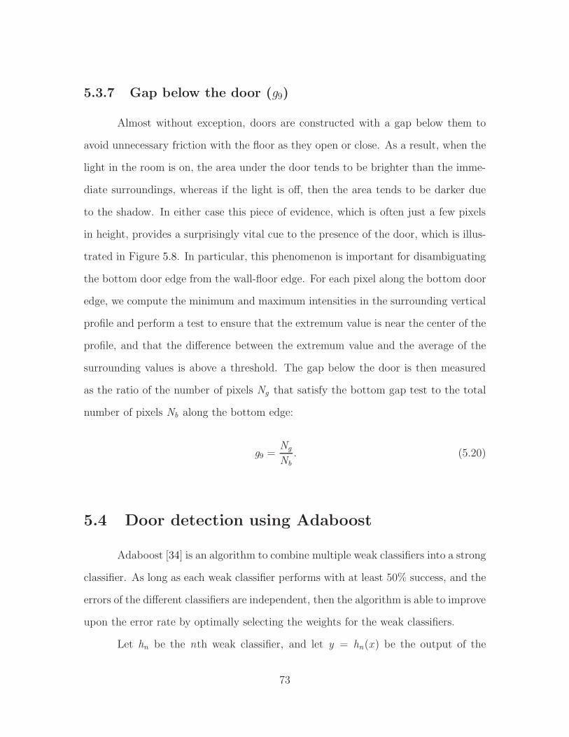
5.3.7 Gap below the door (g9)
Almost without exception, doors are constructed with a gap below them to
avoid unnecessary friction with the floor as they open or close. As a result, when the
light in the room is on, the area under the door tends to be brighter than the imme-
diate surroundings, whereas if the light is off, then the area tends to be darker due
to the shadow. In either case this piece of evidence, which is often just a few pixels
in height, provides a surprisingly vital cue to the presence of the door, which is illus-
trated in Figure 5.8. In particular, this phenomenon is important for disambiguating
the bottom door edge from the wall-floor edge. For each pixel along the bottom door
edge, we compute the minimum and maximum intensities in the surrounding vertical
profile and perform a test to ensure that the extremum value is near the center of the
profile, and that the difference between the extremum value and the average of the
surrounding values is above a threshold. The gap below the door is then measured
as the ratio of the number of pixels Ng that satisfy the bottom gap test to the total
number of pixels Nb along the bottom edge:
g9 =Ng
Nb
. (5.20)
5.4 Door detection using Adaboost
Adaboost [34] is an algorithm to combine multiple weak classifiers into a strong
classifier. As long as each weak classifier performs with at least 50% success, and the
errors of the different classifiers are independent, then the algorithm is able to improve
upon the error rate by optimally selecting the weights for the weak classifiers.
Let hn be the nth weak classifier, and let y = hn(x ) be the output of the
73
0 5 10 15 20 2520
40
60
80
100
120
140
Pixels along the line
Inte
nsity
intensity of pi
0 5 10 15 20 2560
80
100
120
140
Pixels along the lineIn
tens
ity
intensity of pi
0 5 10 15 20 2540
60
80
100
120
140
pixels along the line
Inte
nsity
intensity of pi
Figure 5.8: The intensity profile of a vertical slice around the bottom edge. Left:
images. Top-right: The intensity profile of a vertical slice around the bottomedge. The dark region caused by the shadow of the door indicates the presence ofthe door. Middle-right: Alternatively, if the light in the room is on, a bright peakindicates the door’s presence. Bottom-right: However, if the vertical slice coversthe intersection of the wall and floor, the intensity profile changes smoothly, and nosharp peak occurs.
classifier to input x . In our case, x is the image and y is a binary label indicating
whether a door was detected by the weak classifier. The strong classifier is given by
a weighted sum of the weak classifiers:
Ψ(x ) = sign
(N∑
n=1
αnhn(x )
), (5.21)
74
where αn is the scalar weight found by AdaBoost indicating the importance of the
weak classifier hn , and N = 5. The weights are determined in an iterative manner
according to
αn =1
2
(ln
1− εn
εn
), (5.22)
where the error εn is given by
εn = Pri∼Dn[hn(xi) 6= yi ] =
∑
i :hn (xi )6=yi
Dn(i). (5.23)
In this equation the output yi ∈ {−1, +1} is the ground truth for the training set,
and Dn(i) is the weight assigned to the ith training example on round n.
5.5 Door detection using DDMCMC
Markov Chain Monte Carlo (MCMC) is used here to find the MAP solution
to door detection. Suppose the Markov chain is in state S . We randomly choose a
move of type i , which transforms S to S ′ with proposal probability qi(S → dS ′).
The new state S ′ is then accept with probability based on the Metropolis-Hastings
method,
a(S → dS ′) = min
(1,
E (S ′)qi(S′ | S )
E (S )qi(S | S ′)
). (5.24)
Given current candidate S with state S = (xl , xr , ylt , ylb , yrt , yrb), all parameters change
simultaneously and each parameter has equal chance to update. The speed of a
Markov Chain depends critically on the design of its proposal probabilities in the
jump. If we choose uniform distributions, it is equivalent to blind search and Markov
chain will experience exponential waiting time before each jump. The proposal prob-
75
ability q(s) should be very close to E (S ) within the search space. Therefore, we must
seek approximations and this is where the data-driven methods step in. In data-
driven MCMC, the proposal probability qi(S → dS ′) is changed to qi(S′ | S , I ) and
the new state S ′ is then accept with probability
a(S → dS ′) = min
(1,
E (S ′)qi(S′ | S , I )
E (S )qi(S | S ′, I )
)(5.25)
qi(S′ | S , I ) indicates that we can draw new parameters according to some important
cues in the image. As we mentioned in the previous section, doors appear more
frequently in the image at the position close to the vertical lines which are long
enough. This cue could be used to guide the search of xr , xl . Then the proposal
probability qxi (S ′ | S , I ) for sampling x -coordinates of xr , xl is taken as:
qi(x′ | x , I ) = q(x | l)q(l) (5.26)
where
q(x | l) = − 1
2πδx
exp
{−(x ′ − x ∗)2
2δ2x
}(5.27)
q(l) is the probability to choose the vertical lines in the image. We simply sample
the vertical lines from a uniform distribution. x ∗ is the x -coordinate of the sampled
vertical line.
Because the cameras are low to the ground, the top of the door (the lintel) is
often occluded or a horizontal line Lt closest to the top of the image. The bottom
of the door is often close to the wall/floor boundary Lf . We use these cues to speed
up the jumps of ylt , ylb , yrt , yrb . Let y+k be the y-coordinates of the intersection of
Lt and ℓl , ℓr , and y−k be the y-coordinates of the intersection of Lf and ℓl , ℓr , where
76

k ∈ {l , r}. Then the proposal probability qyi (S ′ | S , I ) for sampling ylt , ylb , yrt , yrb is
taken as:
qi(y′ | y , I ) = − 1
2πδy
exp
{−(y ′ − y∗)2
2δ2y
}(5.28)
where y∗ = y+k , k ∈ {l , r} for updating ylt , yrt and y∗ = y−
k , k ∈ {l , r} for updating
ylb , yrb . y+k = 0 if door is lintel occluded.
When the algorithm rejects proposals by a certain times consecutively, we stop
the algorithm and take the current proposal as the door detected.
All the operations are stochastic, thus the Markov chain designed in this way is
ergodic and aperiodic, i.e., the Markov chain can travel between any state Si and state
Sj in a finite number of steps. This ensures that the chain can reach the maximum
point in the proposal space.
After one proposal is finally determined as a door, our algorithm steps forward
for detecting the next door. The image zone of the detected door will not be searched
for detecting the next door. The detection will stop when the score of the door
candidate is lower than a threshold.
5.6 Acquiring door/wall color model by training
As described above in this section, color is one of the weak classifiers in our
Ababoost-based door detection system. We need to estimate the color histogram of
the wall in advance so that we can compare with the color histogram of the door
candidates. We have developed three methods, either of which can automatically
distinguish wall/door color in an unknown environment.
Method 1: absolute width of door.
77
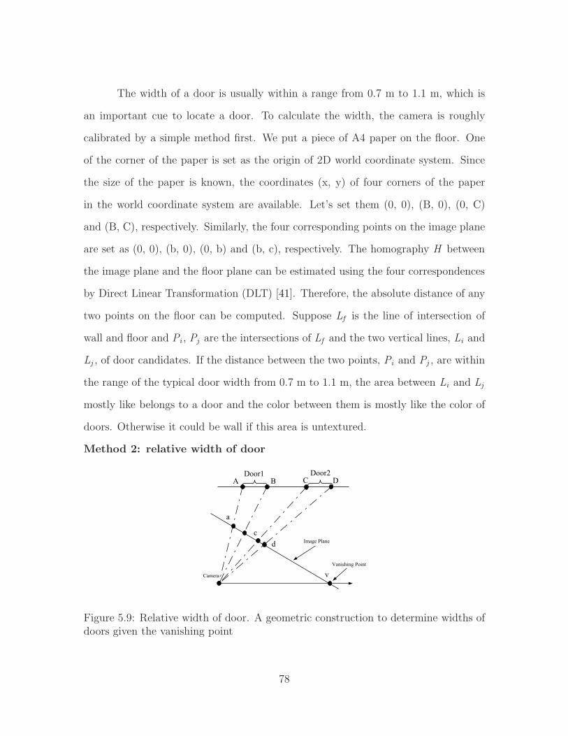
The width of a door is usually within a range from 0.7 m to 1.1 m, which is
an important cue to locate a door. To calculate the width, the camera is roughly
calibrated by a simple method first. We put a piece of A4 paper on the floor. One
of the corner of the paper is set as the origin of 2D world coordinate system. Since
the size of the paper is known, the coordinates (x, y) of four corners of the paper
in the world coordinate system are available. Let’s set them (0, 0), (B, 0), (0, C)
and (B, C), respectively. Similarly, the four corresponding points on the image plane
are set as (0, 0), (b, 0), (0, b) and (b, c), respectively. The homography H between
the image plane and the floor plane can be estimated using the four correspondences
by Direct Linear Transformation (DLT) [41]. Therefore, the absolute distance of any
two points on the floor can be computed. Suppose Lf is the line of intersection of
wall and floor and Pi , Pj are the intersections of Lf and the two vertical lines, Li and
Lj , of door candidates. If the distance between the two points, Pi and Pj , are within
the range of the typical door width from 0.7 m to 1.1 m, the area between Li and Lj
mostly like belongs to a door and the color between them is mostly like the color of
doors. Otherwise it could be wall if this area is untextured.
Method 2: relative width of door
Figure 5.9: Relative width of door. A geometric construction to determine widths ofdoors given the vanishing point
78

Generally, doors have similar widths in an environment. In other words, if
we can find four vertical lines intersecting with floor and the distances between two
of them are similar, the four vertical lines most likely belong two doors. Here we
develop a simple algorithm which can approximately distinguish doors from their
surroundings without calibrating the camera.
As shown in Figure 5.9, (A, B) (C, D) are the intersection points of the floor
and the vertical lines of door 1 and door 2 respectively, (a, b) and (c, d) are the
corresponding points on the image plane. Given the vanishing point, the relative
width of door 1 and door 2 can be computed with Algorithm: DoorWidth
Algorithm: DoorWidth
1. Set the origin of the 1D world coordinate system at A. Then points A B C Dcan be represented as coordinates 0, B, C, D and homogeneous (0, 1), (B, 1),(C, 1) and (D, 1). The vanishing point V can be represented as homogeneous(1, 0).
2. Similarly, set the origin of the 1D image coordinate system at a. Then pointsa b c d can be represented as coordinates 0, b, c, d and homogeneous as (0,1), (b, 1), (c, 1), and (d, 1). The vanishing point v can be represented ascoordinates v and homogeneous (v, 1).
3. There is a 2 × 2 1D prospective transformation H2x2 mapping a → A, b → Bc → C and d → D. Compute the H2x2 by mapping a(0, 1) → A(0, 1) andv(v , 1)→ V(1, 0),
H2x2 =
[1v
0− 1
v1
]
4. The b is known. Therefore, B = H2x2b. Similarly, C and D can be calculated.
5. The relative widths of the two doors are B and D - C, respectively. If B ≈ D -C, (A B) and (C D) construct two doors.
First of all, we find two door candidates by Algorithm: DoorWidth. Second,
the result will be verified by checking the similarity of color between them and the
79
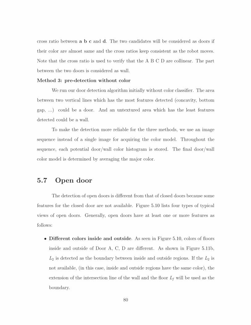
cross ratio between a b c and d. The two candidates will be considered as doors if
their color are almost same and the cross ratios keep consistent as the robot moves.
Note that the cross ratio is used to verify that the A B C D are collinear. The part
between the two doors is considered as wall.
Method 3: pre-detection without color
We run our door detection algorithm initially without color classifier. The area
between two vertical lines which has the most features detected (concavity, bottom
gap, ...) could be a door. And an untextured area which has the least features
detected could be a wall.
To make the detection more reliable for the three methods, we use an image
sequence instead of a single image for acquiring the color model. Throughout the
sequence, each potential door/wall color histogram is stored. The final door/wall
color model is determined by averaging the major color.
5.7 Open door
The detection of open doors is different from that of closed doors because some
features for the closed door are not available. Figure 5.10 lists four types of typical
views of open doors. Generally, open doors have at least one or more features as
follows:
• Different colors inside and outside. As seen in Figure 5.10, colors of floors
inside and outside of Door A, C, D are different. As shown in Figure 5.11b,
L2 is detected as the boundary between inside and outside regions. If the L2 is
not available, (in this case, inside and outside regions have the same color), the
extension of the intersection line of the wall and the floor Lf will be used as the
boundary.
80
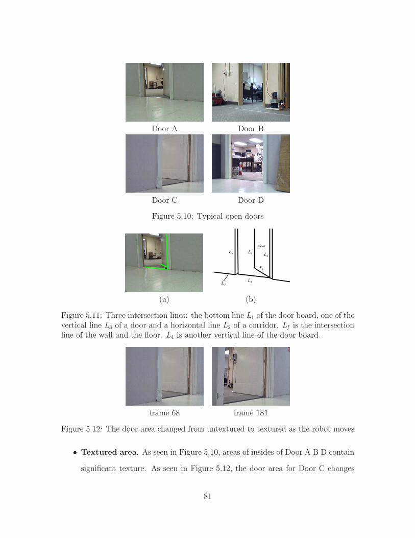
Door A Door B
Door C Door D
Figure 5.10: Typical open doors
(a) (b)
Figure 5.11: Three intersection lines: the bottom line L1 of the door board, one of thevertical line L3 of a door and a horizontal line L2 of a corridor. Lf is the intersectionline of the wall and the floor. L4 is another vertical line of the door board.
frame 68 frame 181
Figure 5.12: The door area changed from untextured to textured as the robot moves
• Textured area. As seen in Figure 5.10, areas of insides of Door A B D contain
significant texture. As seen in Figure 5.12, the door area for Door C changes
81
from untextured to textured as the robot moves over time.
• Three intersection lines. As seen in Figure 5.11, there are three lines inter-
secting in one point; the bottom line of the door board L1 , the vertical line L3
of the door, and the horizontal line L2 of the corridor. This case can be seen
for Door A and C. To decrease the false positive, the following rules have to be
satisfied:
– the angle between L2 and Lf should be smaller than the angle between L1
and Lf .
– another vertical line L4 should either exist (Door A) or overlap with one
of the door post (Door C).
– area between L1, L3 and L4 should be untextured.
• non-coplanar. For an open door, we assume that both posts of the door as
well as the areas near the posts are within a plane, which we call post plane,
while the region between the two posts is located in a different plane. Given
two consecutive image frames, there is a homography mapping the two post
planes. Therefore, any corresponding points or lines on the two post planes
should satisfy the homography, while any corresponding points or lines between
the two posts should not satisfy the homography. The homography is computed
by the normalized extended DLT algorithm [29]. This algorithm uses both point
and line correspondences such that it improves the homography results. The
algorithm is briefly described in Algorithm: Homography. We use joint feature
tracking [13] to obtain point correspondences between images. Using those
feature points on the lines, line correspondences are acquired by least squares
line fitting. Due to the possible errors from the tracker and approximation errors
82
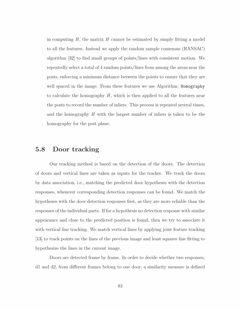
in computing H , the matrix H cannot be estimated by simply fitting a model
to all the features. Instead we apply the random sample consensus (RANSAC)
algorithm [32] to find small groups of points/lines with consistent motion. We
repeatedly select a total of 4 random points/lines from among the areas near the
posts, enforcing a minimum distance between the points to ensure that they are
well spaced in the image. From these features we use Algorithm: Homography
to calculate the homography H , which is then applied to all the features near
the posts to record the number of inliers. This process is repeated several times,
and the homography H with the largest number of inliers is taken to be the
homography for the post plane.
5.8 Door tracking
Our tracking method is based on the detection of the doors. The detection
of doors and vertical lines are taken as inputs for the tracker. We track the doors
by data association, i.e., matching the predicted door hypotheses with the detection
responses, whenever corresponding detection responses can be found. We match the
hypotheses with the door detection responses first, as they are more reliable than the
responses of the individual parts. If for a hypothesis no detection response with similar
appearance and close to the predicted position is found, then we try to associate it
with vertical line tracking. We match vertical lines by applying joint feature tracking
[13] to track points on the lines of the previous image and least squares line fitting to
hypothesize the lines in the current image.
Doors are detected frame by frame. In order to decide whether two responses,
d1 and d2, from different frames belong to one door, a similarity measure is defined
83
Algorithm: Homography
Given n 2D to 2D point correspondences xi ↔ x′i and m 2D to 2D line correspondence
li ↔ l′i , m + n > 4, determine the 2D homography matrix H .
1. Compute a transformation T that maps points xi to xi such that the centroidof the points xi is the coordinate origin and the average distance from the originis√
2, where
T =
s 0 tx0 s ty0 0 1
2. Transform lines li = (a, b, 1) to li ,
li = s
ab
s − txa − tyb
3. Similarly, computer a transformation T ′ by repeating step 1 and step 2 mapping
points x′i to x′
i and transform lines l′i to l′
i .
4. Construct matrix Api by points xi = (xi , yi , 1) and points x′
i = (x ′i , y
′i , 1), Ap
i =
[−xi −yi −1 0 0 0 x ′
ixi x ′iyi x ′
i
0 0 0 −xi −yi −1 y ′ixi u ′
iyi y ′i
]
5. Construct matrix Ali by lines li = (ai , bi , 1) and lines l
′
i = (a ′i , b
′i , 1), Al
i =
[−a ′
i 0 a ′iai −b ′
i 0 b ′iai −1 0 ai
0 −a ′i a ′
ibi 0 −b ′i b ′
ibi 0 −1 bi
]
6. Stack Api on top of Al
i to give a matrix A. Solve equation Ah = 0 by Singular
Value Decomposition (SVD) to get h, and H =
h11 h12 h13
h21 h22 h23
h31 h32 h33
.
Figure 5.13:
as the following likelihood mode:
S (d1, d2) = Spos(d1, d2)Ssize(d1, d2)Scolor (d1, d2), (5.29)
84
where Spos , Ssize , and Scolor are affinities based on position, size, and color of two
detection responses respectively. Their definitions are
Spos(d1, d2) = ηposexp
[−(x1 − x2)
2
σ2x
]exp
[−(y1 − y2)
2
σ2y
], (5.30)
Ssize(d1, d2) = ηsizeexp
[−(x1 − x2)
2
σ2x
], (5.31)
Scolor =
∑N
i=1 min(φ1[i ], φ2[i ])∑N
i=1 φ1[i ](5.32)
where φ1[i ] and φ2[i ] are the numbers of pixels in the ith bin of the histograms of
two detection responses, respectively, and N is the number of bins. ηpos and ηsize are
normalizing factors.
We start to track a door when enough evidence is collected from the detection
responses. If a door has T consecutive detection responses with S (d1, d2) greater
than a threshold, we start to track the door. For a new frame, for all existing doors,
we first look for their corresponding detection responses in this frame. If there is
a new detection response matched with a existing door, then the door location is
updated with the detected door. Otherwise we match the S (d1, d2) of the region
between two tracked vertical lines with a existing door. If S (d1, d2) is greater than
a threshold, the door location is updated with the two tracked vertical lines. When
a door detection responses are not found for consecutive T time steps, the tracking
of the door is terminated.
5.9 Experimental results
To test the performance of the system, we created a database consisting of 577
door images. All the door images was taken in more than twenty different buildings
85

exhibiting a wide variety of different visual characteristics. The images were taken by
an inexpensive Logitech QuickCam Pro 4000 mounted about 30 cm above the floor
on an ActivMedia Pioneer P3AT mobile robot. 100 images were used for training the
algorithm. On the remaining 477 images, which were used for testing, the algorithm
detects 90% of the doors with a false positive rate of 0.07 non-doors per image (on
average) by MCMC and 86% of the doors with a false positive rate of 0.09 non-doors
per image (on average) by DDMCMC. The algorithm was implemented in Visual
C++ and runs at a speed of 5 frame/s on a 1.6 GHz Dell Inspiron 700m laptop
computer.
a) b)
0 20 40 60 800
0.2
0.4
0.6
0.8
1
Iteration
Sco
re
MCMCMCMC + AdaboostDDMCMCDDMCMC + Adaboost
c)
Figure 5.14: Comparison of MCMC and DDMCMC with/without weighting to detectdoors. Data are collected from testing in 10 typical images and averaged. See textfor explanation.
We first show our working example on a simple image. We freely pick two ver-
86
tical lines as an initial guess of a door as shown in Figure 5.14a. We detect the door
by the traditional MCMC and the DDMCMC we proposed above, respectively. For
MCMC, the door is searched with a uniform distribution over the image. Also, the
cues of the door are either treated equally, i.e., αi and βj are set to 1, or weighted by
Adaboost. The score E changes are shown in Figure 5.14c. We can see the DDMCMC
achieves tremendous speedup in comparison to the traditional MCMC. Also we notice
that the Adaboost weighting significantly increases the searching speed for the tradi-
tional MCMC. As for DDMCMC, the Adaboost weighting does not play an important
role at first (scores both change from 0.8 to 0.08 in 2 iterations). That means DDM-
CMC with both weighted and un-weighted models can roughly find the door rapidly.
However, afterward, the score searched by the DDMCMC with a weighted model can
reaches the maximum faster than the DDMCMC with a un-weighted model. Also
we note that since the score sharply drops with DDMCMC and almost reaches the
maximum (from 0.8 to 0.08) in just 2 iterations. We might not have to search the
entire solution space and completely maximize the score so that we can find a door
even faster. Figure 5.15 compares the results. As shown in the top images, there is
no significant difference between the two methods. However, as shown in the bot-
tom images, DDMCMC with 90% maximized score is not able to precisely locate the
door. In our experiments, DDMCMC with 90% maximized score can achiev almost
the same results for around 90% images, and yet the speed is increased 30 times from
0.16 frames/s to 4.2 frames/s.
Figure 5.16 shows some typical doors detected by our system but unsuccess-
fully or incompletely detected by Adaboost algorithm [24]. Our approach can get bet-
ter results because DDMCMC is able to explore the entire solution space and, thus,
achieves a nearly global optimal solution, while the Adaboost-based algorithm [24]
locates doors highly depending on the positions of the detected vertical lines. Line
87
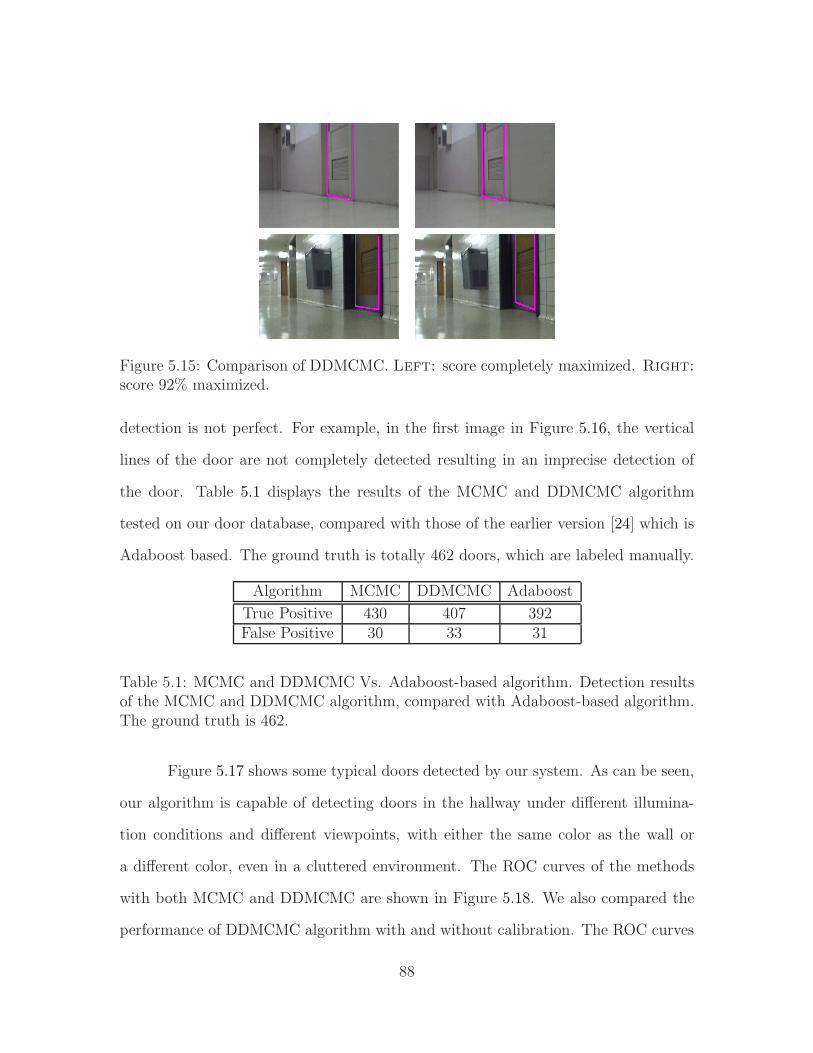
Figure 5.15: Comparison of DDMCMC. Left: score completely maximized. Right:
score 92% maximized.
detection is not perfect. For example, in the first image in Figure 5.16, the vertical
lines of the door are not completely detected resulting in an imprecise detection of
the door. Table 5.1 displays the results of the MCMC and DDMCMC algorithm
tested on our door database, compared with those of the earlier version [24] which is
Adaboost based. The ground truth is totally 462 doors, which are labeled manually.
Algorithm MCMC DDMCMC Adaboost
True Positive 430 407 392False Positive 30 33 31
Table 5.1: MCMC and DDMCMC Vs. Adaboost-based algorithm. Detection resultsof the MCMC and DDMCMC algorithm, compared with Adaboost-based algorithm.The ground truth is 462.
Figure 5.17 shows some typical doors detected by our system. As can be seen,
our algorithm is capable of detecting doors in the hallway under different illumina-
tion conditions and different viewpoints, with either the same color as the wall or
a different color, even in a cluttered environment. The ROC curves of the methods
with both MCMC and DDMCMC are shown in Figure 5.18. We also compared the
performance of DDMCMC algorithm with and without calibration. The ROC curves
88

Adaboost[24] DDMCMC Adaboost[24] DDMCMC
Figure 5.16: Our algorithm vs. Adaboost-based algorithm. Typical doors detectedby our system but unsuccessfully or incompletely detected by Adaboost algorithm.
are shown in Figure 5.19. As can be seen, the calibrated system can achieve higher
true positive rate and lower false positive rate. From the ROC curves of the individual
features shown in Figure 5.20, it is clear that a significant improvement is achieved
by combining all the features. Moreover, the features of color, width, concavity and
gap below the door play an extremely important role compared with other features.
One question arises: are all the features necessary for door detection? Or can
we use fewer features instead of all of them? Performances of feature combinations
are tested to answer these questions. In order to simplify the experiments, we arrange
the features by the importance according to the weights achieved from the Adaboost
89

training as shown in Figure 5.21. Eight combinations are created. For example, K7
combination includes all the features except “kick plate” while K2 includes “width”
and “concavity” only. The ROC curve in Figure 5.22 shows performances of feature
combinations. The equal error rates (EERs) are drawn in Figure 5.23. As can be
seen, the EERs of K5, K6, K7 are almost same (0.05). That means that feature “kick
plate”,“vanishing point”, and “texture” play unimportant roles in door detection.
K5 (width + color + concavity + bottom gap + edge intensity) could achieve results
good enough.
Of course, the system is not perfect, and some errors are shown in Figure 5.24
for completeness.
To demonstrate the utility of the algorithm, we used the robot shown in Fig-
ure 1.3 equipped with two webcams with diverging optical axes. As the robot moved
down a corridor, doors were detected on both sides of the hallway by the algorithm
by processing the images on-line. Doors were tracked from frame to frame. Doors
that were not repeatedly detected a certain number of image frames were regarded
as false positives and discarded.
Figure 5.25 shows the results of five trials in which the robot was manually
driven along approximately the same path at a speed of 0.2 m/s down a 40 m × 15 m
corridor with a 90-degree turn. 25 closed doors in the corridor were detected and
tracked with 100% accuracy, that is, 5 detections out of 5 trials. A door partly
occluded by water fountain is also detected and tracked. However, a cabinet was
detected as two doors mistakenly because it really looks like a double door. Overall,
the detection rate was 100% with a false positive rate of 0.008 per meter driven.
Figure 5.26 shows some typical samples.
Figure 5.27 shows some typical open doors detected by our system and the
ROC curve is shown in Figure 5.28.
90

Figure 5.17: Examples of doors successfully detected by our algorithm. Note thevariety of door widths, door and wall colors, relative pose of the door with respect tothe robot, floor texture, and lighting conditions. Distant doors are not considered bythe algorithm.
5.10 Summary
We have presented a vision-based door detection algorithm based on Data-
Driven Markov Chain Monte Carlo (DDMCMC). Models of doors utilizing a variety
of features, including color, texture, and intensity edges are presented. We intro-
duce two novel geometric features that increase performance significantly: concavity
and bottom-edge intensity profile. The Bayesian formulations are constructed and
a Markov chain is designed to sample proposals. The features are combined using
Adaboost to ensure optimal linear weighting. Doors are detected based on the idea
91
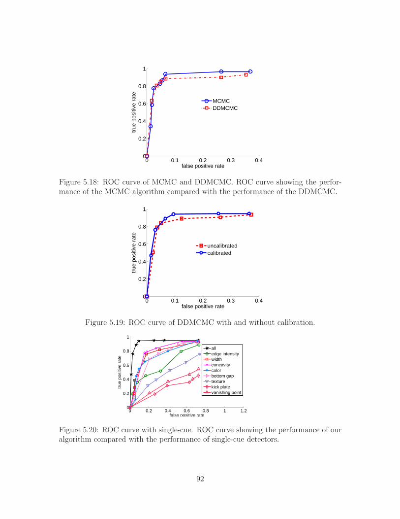
0 0.1 0.2 0.3 0.40
0.2
0.4
0.6
0.8
1
false positive rate
true
pos
itive
rat
e
MCMCDDMCMC
Figure 5.18: ROC curve of MCMC and DDMCMC. ROC curve showing the perfor-mance of the MCMC algorithm compared with the performance of the DDMCMC.
0 0.1 0.2 0.3 0.40
0.2
0.4
0.6
0.8
1
false positive rate
true
pos
itive
rat
e
uncalibratedcalibrated
Figure 5.19: ROC curve of DDMCMC with and without calibration.
0 0.2 0.4 0.6 0.8 1 1.20
0.2
0.4
0.6
0.8
1
false positive rate
true
pos
itive
rat
e
alledge intensitywidthconcavitycolorbottom gaptexturekick platevanishing point
Figure 5.20: ROC curve with single-cue. ROC curve showing the performance of ouralgorithm compared with the performance of single-cue detectors.
92
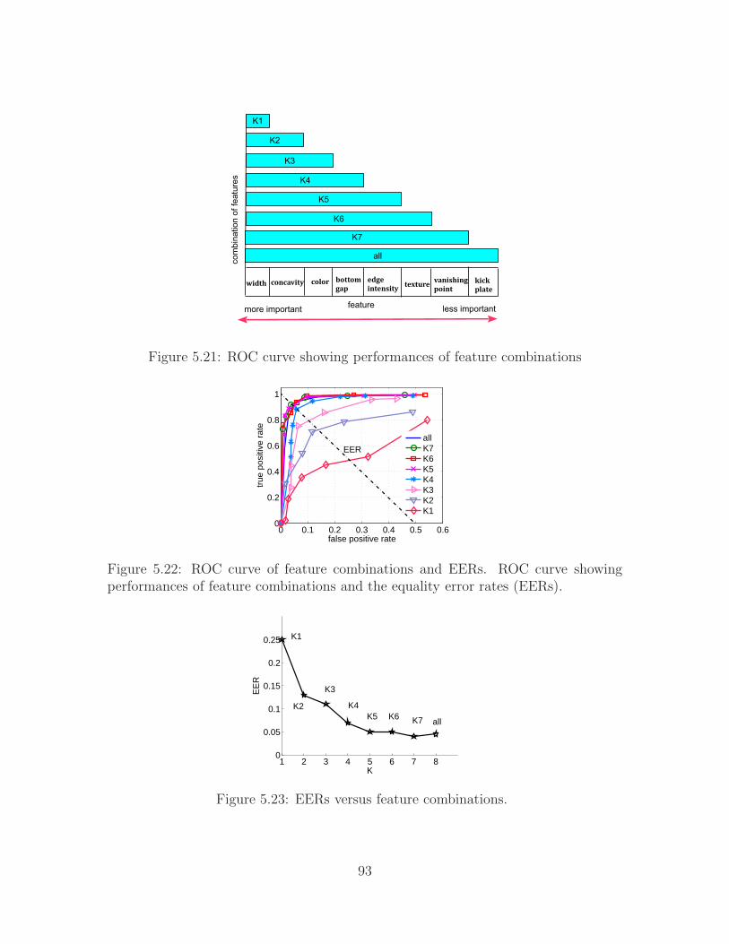
Figure 5.21: ROC curve showing performances of feature combinations
0 0.1 0.2 0.3 0.4 0.5 0.60
0.2
0.4
0.6
0.8
1
false positive rate
true
pos
itive
rat
e
allK7K6K5K4K3K2K1
EER
Figure 5.22: ROC curve of feature combinations and EERs. ROC curve showingperformances of feature combinations and the equality error rates (EERs).
1 2 3 4 5 6 7 80
0.05
0.1
0.15
0.2
0.25
K
EE
R
K1
K2
K3
K4K5 K6 K7 all
Figure 5.23: EERs versus feature combinations.
93
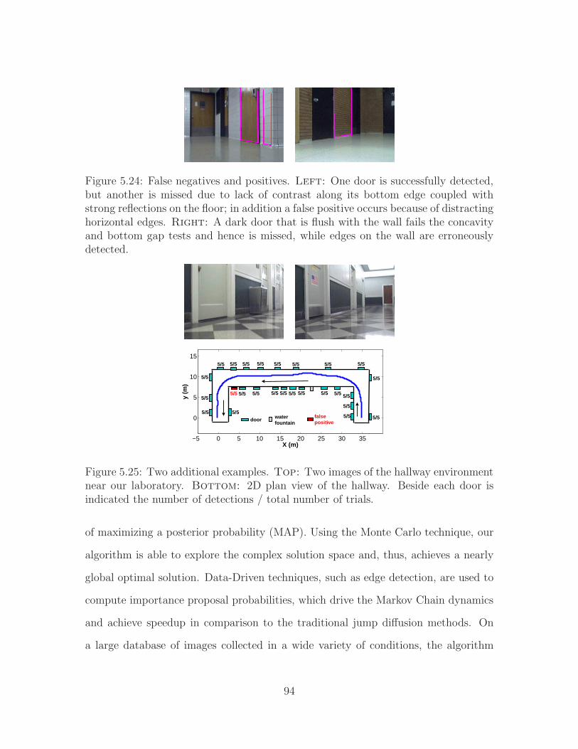
Figure 5.24: False negatives and positives. Left: One door is successfully detected,but another is missed due to lack of contrast along its bottom edge coupled withstrong reflections on the floor; in addition a false positive occurs because of distractinghorizontal edges. Right: A dark door that is flush with the wall fails the concavityand bottom gap tests and hence is missed, while edges on the wall are erroneouslydetected.
−5 0 5 10 15 20 25 30 35
0
5
10
15
X (m)
y (m
)
door waterfountain
5/5
5/5
5/5
5/5
5/5
5/5
5/55/5
5/55/55/55/55/55/55/5
5/55/5
5/5
5/5
5/5 5/5 5/5 5/5 5/5 5/5
5/5
falsepositive
Figure 5.25: Two additional examples. Top: Two images of the hallway environmentnear our laboratory. Bottom: 2D plan view of the hallway. Beside each door isindicated the number of detections / total number of trials.
of maximizing a posterior probability (MAP). Using the Monte Carlo technique, our
algorithm is able to explore the complex solution space and, thus, achieves a nearly
global optimal solution. Data-Driven techniques, such as edge detection, are used to
compute importance proposal probabilities, which drive the Markov Chain dynamics
and achieve speedup in comparison to the traditional jump diffusion methods. On
a large database of images collected in a wide variety of conditions, the algorithm
94

Figure 5.26: Door detection and tracking in a hallway.
Figure 5.27: Detecting open doors.
0 0.2 0.4 0.6 0.80
0.2
0.4
0.6
0.8
1
false positive rate
true
pos
itive
rat
e
Figure 5.28: ROC curve of detecting open doors.
achieves more than 90% detection with a low false positive rate. Additional experi-
ments demonstrate the suitability of the algorithm for real-time applications using a
mobile robot equipped with an off-the-shelf camera and a laptop.
95
Chapter 6
Conclusion and Future work
The goal of this dissertation is to endow robots with visual capabilities in
order to make them more autonomous. We proposed three algorithms involving three
important areas in robotics: path following, person following, and door detection, to
solve common problems in the real-world application of robot vision. For any mobile
robot, navigating in its environment is one of the most important capabilities of
all. Our research on path following for mobile robot navigation enables a mobile
robot to determine its own position in its frame of reference and then to plan a path
towards some goal location. Our research on person following is related to human-
robot interaction study. The ability of a mobile robot to follow a person would
benefit applications of using robot as a personal digital assistant in everyday life.
Detection of doors is also one of the important capabilities for an autonomous robot,
and will also benefit other robotics researches, such as building a geometric map
in an indoor environment using doors as landmarks. For the path following, doors
could also be used as significant landmarks in an untextured environment with fewer
reliable feature points. In the future, the three algorithms could be integrated into a
robot navigation system toward fully autonomous robot applications. For example,
96
autonomous robot is highly desired in the hospital distribution service for decreasing
operating costs while improving delivery performance. To meet the delivery needs of
a hospital, any automated solution will need to handle routine deliveries as well as
be flexible enough to handle arbitrary deliveries or other exceptions to the norm [76].
For routine pick-ups and deliveries, the robot follows a predefined route to deliver
supplies to and from the service units. Beside routine deliveries, sometime the robot
needs to deliver items to specific rooms. Therefore, door detection and recognition
are required. For arbitrary deliveries, the robot could follow a hospital staff to deliver
emergent supplies anywhere as required.
Chapter 1 opened with an introductory discussion to motivate and contextual-
ize our research. The importance of vision-based mobile robot sensing was discussed,
and it was concluded that vision sensing is one of the most powerful perception mech-
anisms for robotics. In addition a preview of our research was presented across the
areas of path following, person following, and door detection. In Chapter 2 we moved
on to discuss related work, and reviewed the application of computer vision in three
areas above. Also discussed are some issues in their approaches. Then overviews of
our approaches, and their advantages are described .
Map-based approaches to path following are using calibrated cameras in gen-
eral. However, the camera has to be well calibrated and the ground is assumed
locally planar and horizontal at the current position of the robot. Also they have
to relate the image coordinates to world coordinates or image coordinates between
image frames, which make solutions to path following complicated. In Chapter 3 we
have developed a simple mapless approach to the problem using a single off-the-shelf
camera with no calibration. The algorithm is qualitative in nature, requiring no map
of the environment, no image Jacobian, no homography, no fundamental matrix, and
no assumption about a flat ground plane.
97
Appearance-based approaches for person following have their limitations in
real-world applications. The tracker is easily distracted by environment resulting
in unreliable tracking. In Chapter 4 we have presented a Binocular Sparse Feature
Segmentation (BSFS) algorithm for vision-based person following by fusing motion
and stereo information. This system is able to reliably follow a person in complex
dynamic, cluttered environments in real time.
Previous researches on door detection usually rely on range sensors or combine
the range sensors with vision, and only a few of features (edges, color, or corners of
door) are involved. Therefore, they are limited in handling a variety of challenging
environmental conditions (changing pose, similarly colored doors and walls, strong
reflections, and so forth). We believe that multiple vision cues are necessary for ro-
bustness. In Chapter 5 we have presented a solution to the problem based upon
combining multiple cues. Our approach augments standard features such as color,
texture, and vertical intensity edges with novel geometric features such as the concav-
ity of the door and the gap below the bottom door edge. This algorithm can detect
doors in a variety of challenging environmental conditions, achieving a nearly global
optimal solution in many cases.
In this chapter, the three algorithms will be summarized. Their drawbacks
and future work are also presented.
6.1 Path following
We have presented a novel approach to the problem of vision-based mobile
robot path following using a single off-the-shelf camera. The robot navigates by
performing a qualitative comparison of feature coordinates across the teaching and
replay phases, utilizing the novel concept of a funnel lane. Vision information is
98
combined with odometry for increased robustness. The algorithm does not make
use of the traditional concepts of Jacobians, homographies, fundamental matrices,
or the focus of expansion, and it does not require any camera calibration, including
lens calibration. It only requires implicit calibration in the form of a controller gain.
Experimental results on both indoor and outdoor scenes demonstrate the effectiveness
of the approach on trajectories of hundreds of meters, along with its robustness to
effects such as dynamic objects, slanted surfaces, and rough terrain. The versatility
of the algorithm in working with wide-angle and omnidirectional cameras with only
minor modification has also been shown.
The algorithm is not perfect, and there are scenarios in which it will fail. For
example, occasionally the algorithm does not properly transition to the next milestone
image, in which case the overlap between the current and milestone image can decrease
to the point that an insufficient number of features are matched. Also, untextured
scenes containing distant trees, bushes, or undecorated indoor hallways sometimes
prevent the KLT algorithm from successfully tracking enough features to accurately
compute the heading direction. While only a handful of features are necessary for the
algorithm to succeed, it is important that features exist on both sides of the image,
and that some number of features remain visible throughout the milestone.
Another source of error is due to distant features. Although features near
the center of the image produce a narrow funnel lane even when they are far from
the camera, distant features near the side of the image produce much larger funnel
lanes which are less useful for navigation. Moreover, image parallax is inversely
proportional to the distance to a feature. As a result, distant features are primarily
useful for correcting the rotation of the robot and are quite incapable of informing the
robot about minor translation errors. This problem is compounded by the inherent
ambiguity between rotation and translation in the funnel lane itself. Even though
99
this ambiguity has little effect when the robot is near the path, it hinders the ability
of the visual information to correctly determine the correct amount of rotation when
the robot has deviated significantly. Odometry helps to overcome this limitation, and
we have conducted experiments in which the robot consistently returns to the path
after deviating by several meters. However, much larger deviations either initially or
during replay cannot be handled by our present system. At any rate, it should be
noted that odometry drift is not an issue because we only store odometry values local
to the segment, not in a global coordinate frame.
Because our system does not explicitly model the geometric world, its geo-
metric accuracy is limited. Therefore, when compared with map-based approaches
using calibrated cameras [78], the errors exhibited by the simple control scheme of
our algorithm are rather large. Nevertheless, the remarkable flexibility and versatility
of the system offer some important advantages over more precise techniques. With
our approach, one can literally take an off-the-shelf camera, attach it to the robot,
align it approximately in the forward direction, and start the system.
Since the algorithm depends on comparing scenes between the teaching and re-
play phase, it would fail if the scene changes significantly after teaching. For example,
the robot is taught in a parking lot with a lot of cars parking there in the morning.
And it would fail to repeat the learned path in the afternoon because most cars are
gone. Future work should be aimed at incorporating higher-level scene knowledge to
have the robot focus on those unchanged landmarks, such as buildings, by applying
scene segmentation algorithm.
100
6.2 Person following
We have presented a novel algorithm, called Binocular Sparse Feature Segmen-
tation (BSFS), for vision-based mobile robot person following. The algorithm detects
and matches feature points between a stereo pair of images and between successive
images in the sequence in order to track 3D points in time. Segmentation of the fea-
tures is accomplished through a RANSAC-based procedure to estimate the motion of
each region, coupled with a disparity test to determine the similarity with the target
being tracked. The BSFS algorithm is augmented with the Viola-Jones face detector
for initialization and periodic feature pruning.
This system does not require the person to wear a different color from the
background, and it can reliably track a person in an office environment, even through
doorways, with clutter, and in the presence of other moving objects. However, re-
lying only upon sparse features makes the system subject to distraction by other
objects with similar motion and disparity to the person being tracked. More robust
performance could be achieved by fusing the information used by this algorithm with
additional appearance-based information such as a template or other measure of im-
age intensities or colors. Another limitation of the present system is its inability to
handle the situation when the person leaves the field of view of the camera, or when
another object completely occludes the person, in which case the robot tends to fixate
on the distracting object. A pan-tilt camera or a wider field of view would overcome
this problem. Finally, future should should be aimed at incorporating the proposed
technique with other sensor modalities such as color information, infrared data, or
range sensors to increase robustness [66].
101
6.3 Door detection
We have presented a vision-based door detection algorithm for robot naviga-
tion using an uncalibrated camera. The doors are detected by a camera mounted on
a mobile robot, from which low vantage point the lintel is often not visible. Door
candidates are first sought by detecting the vertical lines that form the door frame,
and then by applying constraints such as size, direction, and distance between seg-
ments. Within these door candidates, several features are measured. The algorithm
augments standard features such as color, texture, and vertical intensity edges with
novel geometric features based on the concavity of the door and the gap below the
bottom door edge. The features are combined in an Adaboost framework to enable
the algorithm to operate even in the absence of some cues. Tested on a large database
exhibiting a wide variety of environmental conditions and viewpoints, the algorithm
achieves more than 90% detection rate with a low false positive rate. The approach
is suitable for real-time mobile robot applications using an off-the-shelf camera, and
preliminary experiments demonstrate the success of the technique.
There is plenty of room for future work in this area. Additional features can
be incorporated into the Adaboost framework to increase performance. Calibration
of the camera, along with 3D line estimation, would enable pose and distance mea-
surements to facilitate the building of a geometric map. In addition, open and closed
doors can be distinguished using motion information inside the door, specifically the
motion parallax of features inside the room that are visible when the door is open.
Finally, the algorithm will be integrated into a complete navigation system that is
able to drive down a corridor and turn into a specified room.
102

Appendices
103

Appendix A
The Kanade-Lucas-Tomasi (KLT)
Feature Tracker
In 1981, Lucas and Kanade [61] proposed a new optical estimation method
that makes use of the spatial intensity gradient of the images to find a good match
between two consecutive images. This method measures the sum of squared intensity
differences between the past and current frame over fixed-size feature windows. The
displacement is then iteratively determined by minimizing this sum using Newton-
Raphson style minimization. In 1991, Tomasi and Kanade [95] improved the technique
by proposing a more principled way to select good features for more reliable feature
tracking. However, this method considered the image motion in 2D so that only a
pure translation model is used during tracking, which results in false tracks for some
“bad” features. In 1994, Shi and Tomasi [84] combined the pure tranlation-based
motion model for feature tracking, with an affine-transformation-based motion model
(linear warping and translation) for image matching. It was proved that false tracks
could be reliably rejected by affine motion model. This is the well-known Kanade-
Lucas-Tomasi (KLT) Feature Tracker. Since then, the KLT algorithm has become
104
one of the most widely used techniques in computer vision to estimate the optical
flow.
A.1 Feature tracking
Let I and J be two consecutive grayscaled images. A point or feature x =
(x , y) measured with respect to a fixed-size window’s center in J moves to point
Ax + d in I , where A is a warp matrix which takes the pixel x in image J and maps
it to image I and the displacement d = (dx , dy). Then
I (Ax + d) = J (x) + n(x), (A.1)
where n(x) is noise. If we consider only a pure translation model, A is equal to the
identity matrix. Then equation (A.1) becomes:
I (x + d) = I (x) + n(x), (A.2)
The problem of feature tracking is determined by finding d that minimize the residue
error over the given window W :
ǫ =
∫
W
[I (x + d)− J (x)]2 w(x)dx, (A.3)
where w is a weighting function. In the simplest case, w(x) could be set to 1. Al-
ternatively, w could be a Gaussian-like function, to emphasize the central area of the
window. When the displacement vector is small, J (x + d) can be approximated by
its Taylor series truncated to the linear term: [61]
105
I (x + d) ≈ I (x) + dx
∂I
∂x(x) + dy
∂I
∂y(x) (A.4)
Differentiating the last expression of the residue ǫ in equation (A.3) with re-
spect to d:
∂ǫ
∂d= 2
∫
W
[I (x + d)− J (x)]
[∂I (x + d)
∂d− ∂J (x)
∂d
]w(x)dx
≈ 2
∫
W
[I (x)− J (x) + gd] gw(x)dx,
where g = (gx , gy) =(
∂∂x
I (x), ∂∂y
I (x)). To find the displacement d, the derivative is
set to zero:
∫
W
[I (x)− J (x) + g · d] gw(x)dx = 0, (A.5)
Rearranging terms, we get
(∫
W
ggTw(x)dx
)d =
∫
W
(J (x)− I (x))gw(x)dx (A.6)
which can be rewritten as
Gd = e, (A.7)
where G =
gxx gxy
gxy gyy
is the following 2 X 2 symmetric coefficient matrix,
G =
∫
W
ggTw(x)dx =∑
W
g2x gxgy
gxgy g2y
(A.8)
106
and e is the following 2× 1 error vector:
e =
∫
W
(J (x)− I (x))gw(x)dx. (A.9)
For every pair of adjacent frames, the matrix G can be computed from one frame,
by estimating gradients and computing their second order moments. The vector e,
on the other hand, can be computed from the difference between the two frames,
along with the gradient computed above. The displacement d is then the solution
of equation (A.7). The solution d to equation (A.7) will usually contain some error.
In practice, equation (A.7) is repeatly solved and x is updated as shown in equation
(A.10) at each iteration until d is less than an accuracy threshold.
x← x + d (A.10)
In general, dx , dy could not be integers during iteration. In order to achieve
high tracking accuracy, bilinear interpolation [15] is used to compute image value at
locations between integer pixels. Let α and β be the two remainder values (between
0 and 1) such that:
x = x0 + α (A.11)
y = y0 + β (A.12)
then,
I (x , y) = (1− α)(1− β)I (x0, y0) + α(1− β)I (x0 + 1, y0) +
(1− α)βI (x0, y0 + 1) + αβI (x0 + 1, y0 + 1). (A.13)
107

A.2 Feature Detecting
A feature point can be tracked only if the equation (A.7) can be solved reliably.
That requires the 2×2 coefficient matrix G must be both above the image noise level
and well conditioned. Tomasi and Kanade [95] pointed out that this requirement can
be satisfied if both eigenvalues λ1, λ2 of G are large enough, i.e.
min(λ1, λ2) > threshold. (A.14)
Two small eigenvalues mean the window belongs to a relatively uniform area and it’s
hard to extract useful motion information. A large and a small eigenvalue usually
means the window is on a straight line and suffers from so called “aperture problem”.
Two large eigenvalues can represent corners or any other highly textured regions that
can be tracked reliably. Since G =
gxx gxy
gxy gyy
, the eigenvalues are calculated by
λ =1
2
[(gxx + gyy)±
√(gxx − gyy)2 + 4g2
xy
](A.15)
To avoid redundant tracking, the minimum distance is enforced so that distance
between any pair of selected features is larger than a given threshold, 5 - 10 pixels
usually.
A.3 Dissimilarity checking
Although the KLT algorithm proposes a criterion, which is optimal by con-
struction, to select good features for tracking, bad features are still often selected due
to the complexities of environments. Actually, even a region with rich texture content
might be poor. For instance, boundaries of different surfaces in the world could inter-
108
sect each other in the image and then produce “bad” feature points, which actually
correspond to no physical points. Also the standard KLT algorithm typically relies
on a constant scene appearance over all view points. This fundamental assumption
is violated for complex environments containing reflections and semi-transparent sur-
faces. Since the feature residue error, sometimes called feature dissimilarity, qualifies
how much the appearance of a feature changes, it has to be well measured so that
“bad” features can be properly removed during tracking. Shi and Tomasi [84] pointed
out that the pure translation mode is not adequate for image motion when measuring
dissimilarity, but affine warping is adequate. Their approach is briefly described as
follows.
Consider an affine motion model, the warping matrix A becomes:
A = I + D (A.16)
where I is the identity matrix and D is the deformation matrix:
D =
Dxx Dxy
Dyx Dyy
(A.17)
Then equation (A.3) that measures the residue error can be replaced by
ǫ =
∫
W
[I (Ax + d)− J (x)]2 w(x)dx, (A.18)
Differentiate it with respect to Dxx ,Dxy ,Dyx ,Dyy and d and set the result to zero, we
have:
Tz = a, (A.19)
109
where T is the following coefficient matrix:
T =
∫
W
x 2g2x x 2gxgy xyg2
x xygxgy xg2x xgxgy
x 2gxgy x 2g2y xygxgy xyg2
y xgxgy xg2y
xyg2x xygxgy y2g2
x y2gxgy yg2x ygxgy
xygxgy xyg2y y2gxgy y2g2
y ygxgy yg2y
xg2x xgxgy yg2
x ygxgy g2x gxgy
xgxgy xg2y ygxgy yg2
y gxgy g2y
w(x)dx, (A.20)
and e is the following error vector:
a =
∫
W
(J (x)− I (x))
xgx
xgy
ygx
ygy
gx
gy
w(x)dx, (A.21)
and z = (Dxx ,Dxy ,Dyx ,Dyy , dx , dy)T
Is affine motion model more reliable to apply for tracking? Many people
have made that observation that it’s actually worse than pure translation model. In
fact, the reason is that affine tracking requires to estimate a very large number of
parameters: 6 instead of 2 for the pure translation model, therefore more error would
be introduced. Another reason might lie in the size of the feature window. The
quality of the tracking depends on the size of the feature window. Small windows
are preferable for tracking because they are more likely to contain features at similar
depths. However, when the window is small, the deformation matrix D is harder to
110
estimate, because the variations of motion within it are smaller and therefore less
reliable.
Since motion between adjacent frames is small during tracking, the affine de-
formation D of the feature window is likely to be the zero matrix. A pure translation
model is thus good enough for tracking while affine motion should only be consid-
ered for building a reliable rejection scheme. During tracking, the equation (A.19) is
solved and the results are used for calculating the dissimilarity by equation (A.18).
If the dissimilarity of the tracked feature point is larger than a threshold, the point
is declared “lost”.
A.4 Pyramidal Implementation
Tracking feature by minimizing the residue error is an ill-posed problem, since
the optimum might be attained by many dissimilar displacement fields. When mo-
tions between two successive frames are larger than one pixel, the minimization algo-
rithm could easily be trapped in a local minimum.
In order to find the global minimum to support large motion and for improved
accuracy, it is useful to apply multiscale coarse-to-fine approach: displacement can
be estimated at the coarsest level of a pyramid, where the image is significantly
blurred, and the velocity is much slower. The coarse solution is then used as initial
guess for the pixel displacement at a finer level of the pyramid. This coarse-to-
fine estimation continues until the finest level of the pyramid (the original image) is
reached. The pyramid height Lm should be picked appropriately according to the
maximum expected optical flow in the image. Each level L of the pyramid is the
downsampling by 2 from the beneath level L−1 after a low pass filter used for image
anti-aliasing.
111

In 1999, Bouguet [15] proposed a implementation which can be found in the
OpenCV library. Let I 0 = I be the 0th level image, the highest resolution image,
L = 1, 2, ...Lm be a pyramidal level. Denote I L the image at level L. The image I L is
then defined as
I L(x , y) =1
4I L−1(2x , 2y) +
1
8
(I L−1(2x − 1, 2y) + I L−1(2x + 1, 2y)
)+
1
8
(I L−1(2x , 2y − 1) + I L−1(2x , 2y + 1)
)+
1
16
(I L−1(2x − 1, 2y − 1) + I L−1(2x + 1, 2y + 1)
)+
1
16
(I L−1(2x + 1, 2y − 1) + I L−1(2x − 1, 2y + 1)
). (A.22)
Let dL be the displacement computed at level L, dL−1 = 2dL. The solution of the
displacement d for the original image is therefore:
d =
Lm∑
L=0
2LdL, (A.23)
A.5 Summary
The entire KLT tracking algorithm are summarized in a form of pseudo-code
.
112
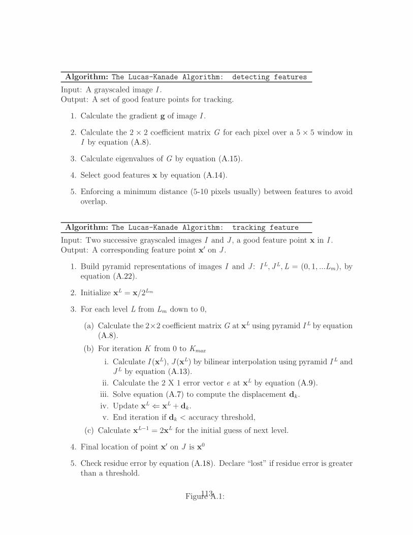
Algorithm: The Lucas-Kanade Algorithm: detecting features
Input: A grayscaled image I .Output: A set of good feature points for tracking.
1. Calculate the gradient g of image I .
2. Calculate the 2 × 2 coefficient matrix G for each pixel over a 5× 5 window inI by equation (A.8).
3. Calculate eigenvalues of G by equation (A.15).
4. Select good features x by equation (A.14).
5. Enforcing a minimum distance (5-10 pixels usually) between features to avoidoverlap.
Algorithm: The Lucas-Kanade Algorithm: tracking feature
Input: Two successive grayscaled images I and J , a good feature point x in I .Output: A corresponding feature point x′ on J .
1. Build pyramid representations of images I and J : I L, JL,L = (0, 1, ...Lm), byequation (A.22).
2. Initialize xL = x/2Lm
3. For each level L from Lm down to 0,
(a) Calculate the 2×2 coefficient matrix G at xL using pyramid I L by equation(A.8).
(b) For iteration K from 0 to Kmax
i. Calculate I (xL), J (xL) by bilinear interpolation using pyramid I L andJL by equation (A.13).
ii. Calculate the 2 X 1 error vector e at xL by equation (A.9).
iii. Solve equation (A.7) to compute the displacement dk .
iv. Update xL ⇐ xL + dk .
v. End iteration if dk < accuracy threshold,
(c) Calculate xL−1 = 2xL for the initial guess of next level.
4. Final location of point x′ on J is x0
5. Check residue error by equation (A.18). Declare “lost” if residue error is greaterthan a threshold.
Figure A.1:113

Appendix B
Line Detection
To detect lines, intensity edges are first detected throughout the image using
the Canny edge detector [20]. To group the edges into straight line segments, many
existing approaches apply the Hough transform, but in our experiments we found this
approach to be quite sensitive to the window size: Small windows cause unwanted
splitting of lines, while large windows cause unwanted merging of lines.
Instead, we employ a modified form of the split-and-merge algorithm developed
by Douglas and Peucker [28], which is shown as the algorithm LineDetection. In
the first step, edge pixels are searched in order to label connected edges. Edges are
divided by junction points, which are defined as edge pixels that are connected to
more than two other pixels in their 8-neighborhood. Small isolated edges and spurs
(short sequences of pixels jutting to the side of the main branch of the edge) are
eliminated.
The second step divides the connected edges into sequences of straight line
segments using a divide-and-conquer strategy. A straightness test is recursively ap-
plied to the edge, stopping when all segments pass the test. In Douglas and Peucker’s
algorithm, the threshold for the maximum allowed deviation dallowed is a constant,
114

which mistakenly absorbs short line segments into long line segments and mistakenly
divides long line segments into multiple short segments. Our modified version of the
algorithm solves this problem by determining dallowed using a half-sigmoid function:
dallowed (s) = δ
(β − e−|s|
β + e−|s|
), (B.1)
where | s | is the length of segment s , δ is a constant specifying the value of dallowed
for long segments, and β > 1 is a constant to increase the slope of the half-sigmoid
function. This function is shown in Figure B.2, and the improvement from the mod-
ification is shown in Figure B.3.
Figure B.4a shows a typical result from this algorithm. Although straight line
segments are found, several problems remain. For example, vertical lines correspond-
ing to the door frame are often broken by door hinges or knobs. In addition, the
reflection of the door creates spurious lines on the floor, often with a gap between
the spurious lines and the true lines. To overcome these problems, we merge vertical
lines separated by a small gap, discard lines that do not extend above the vanishing
point, discard short lines, and retain only lines whose orientation is nearly vertical.
The result of these tests is shown in Figure B.4b.
115

Algorithm: LineDetection
Input: Intensity edges of an imageOutput: A set of straight line segments
1. Edge labeling: For each unlabeled edge pixel
(a) Track edge to find the rest of the connected edge points and label them,stopping if a junction point is encountered
(b) Eliminate isolated edges and spurs that are below the minimum length
2. Line segmenting: For each labeled edge
(a) Create a virtual straight line by connecting the start and end points oflabeled edge
(b) Calculate the deviation (perpendicular distance to the virtual line) of eachpoint on the labeled edge
(c) Divide the virtual line in half at the point of maximum deviation if themaximum deviation is greater than a threshold dallowed
(d) Repeat above process until the maximum deviation of all the line segmentsis less than dallowed
3. Line merging: For each line segment
(a) Merge with another line segment if the maximum tolerated angle deviationbetween them and the maximum distance between their end points arewithin a limit
Figure B.1:
116

0 20 40 60 80 1000
0.5
1
1.5
2
2.5
length of segment
d allo
wed
( p
ixel
)
Figure B.2: The half-sigmoid function of dallowed , which makes the threshold depen-dent upon the length of the segment. δ = 2 and β = 10.
Figure B.3: Modified Douglas-Peucker algorithm. Left: The original algorithmmistakenly absorbs the door recession into segment a, and it mistakenly divides thesingle wall/floor line into b and c. Right: With our modification, the recession isdetected separately as segment B, and the segments b and c are correctly detected asa single segment C. Note that the recession segment B is important for the concavitytest described in Section 5.3.6.
117
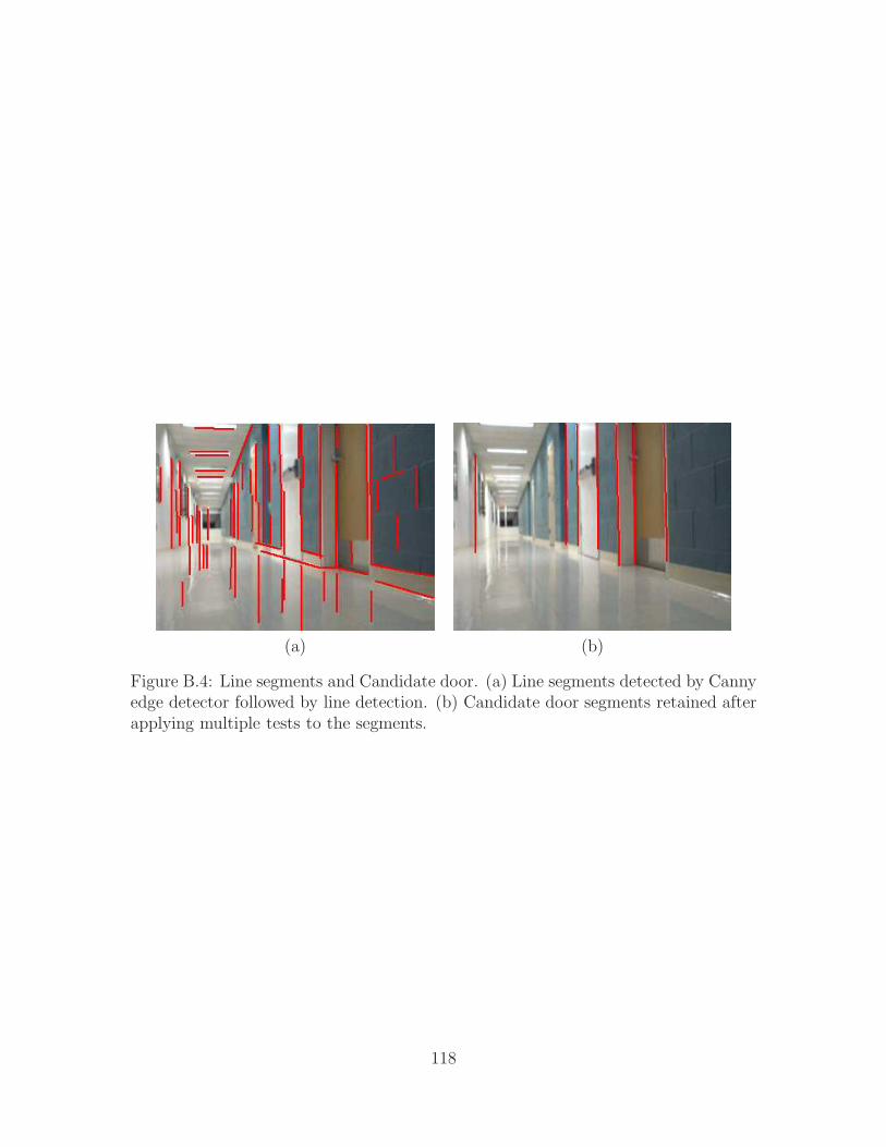
(a) (b)
Figure B.4: Line segments and Candidate door. (a) Line segments detected by Cannyedge detector followed by line detection. (b) Candidate door segments retained afterapplying multiple tests to the segments.
118

Bibliography
[1] OpenCV library, http://sourceforge.net/projects/opencvlibrary/files/.
[2] C. Ackerman and L. Itti. Robot steering with spectral image information. IEEETransactions on Robotics, 21(2):247–251, Apr. 2005.
[3] G. Adorni, S. Cagnoni, M. Mordonini, and A. Sgorbissa. Omnidirectional stereosystems for robot navigation. In Proceedings of the Fourth Workshop on Om-nidirectional Vision (Omnivis), 2003.
[4] D. Anguelov, D. Koller, E. Parker, and S. Thrun. Detecting and modeling doorswith mobile robots. In Proceedings of the IEEE International Conference onRobotics and Automation, 2004.
[5] G. C. Anousaki and K. J. Kyriakopoulos. Simultaneous localization and mapbuilding for mobile robot navigation. IEEE Robotics and Automation Magazine,6(3):42–53, Sept. 1999.
[6] S. Atiya and G. D. Hager. Real-time vision-based robot localization. IEEETransactions on Robotics and Automation, 9(6):785–799, Dec. 1993.
[7] S. Baker and I. Matthews. Optimal landmark configuration for vision-basedcontrol of mobile robots. International Journal of Computer Vision, 56(3):221–255, 2004.
[8] R. Barber, M. Mata, M. Boada, J. Armingol, and M. Salichs. A perceptionsystem based on laser information for mobile robot topologic navigation. InThe 28th Annual Conference of the IEEE Industrial Electronics Society, 2002.
[9] R. Barnes. Motion and time study: design and measurement of work. JohnWiley and Sons Inc, 7th edition, 1980.
[10] G. L. Barrows, J. S. Chahl, and M. V. Srinivasan. Biomimetic visual sensingand flight control. In Bristol Conference on UAV Systems, 2002.
[11] D. Beymer and K. Konolige. Tracking people from a mobile platform. Interna-tional Joint Conference on Artificial Intelligence, 2001.
119

[12] S. Birchfield, 1997. KLT: An implementation of the Kanade-Lucas-Tomasi fea-ture tracker, http://www.ces.clemson.edu/˜stb/klt/.
[13] S. T. Birchfield and S. J. Pundlik. Joint tracking of features and edges. Pro-ceedings of the IEEE Conference on Computer Vision and Pattern Recognition(CVPR), 2008.
[14] J. Borenstein, H. R. Everett, L. Feng, and D. Wehe. Mobile robot positioning:Sensors and techniques. Journal of Robotic Systems, 14(4):231–249, Apr. 1997.
[15] J.-Y. Bouguet. Pyramidal implementation of the Lucas Kanade feature tracker.OpenCV documentation, Intel Corporation, Microprocessor Research Labs,1999.
[16] W. Burgard, A. B. Cremers, D. Fox, D. Hahnel, G. Lakemeyer, D. Schulz,W. Steiner, and S. Thrun. Experiences with an interactive museum guide-robot. Artificial Intelligence, 114(1-2):3–55, 1999.
[17] W. Burgard, D. Fox, D. Hennig, and T. Schmidt. Estimating the absoluteposition of a mobile robot using position probability grids. In Proceedings ofthe National Conference on Artificial Intelligence, 1996.
[18] D. Burschka and G. Hager. Vision-based control of mobile robots. In Proceedingsof the International Conference on Robotics and Automation, pages 1707–1713,May 2001.
[19] D. Burschka and G. D. Hager. V-GPS (SLAM): Vision-based inertial systemfor mobile robots. In Proceedings of the International Conference on Roboticsand Automation, pages 409–415, Apr. 2004.
[20] J. F. Canny. A computational approach to edge detection. IEEE Transactionson Pattern Analysis and Machine Intelligence, 8(6):679–698, 1986.
[21] B. Cartwright and T. Collett. Landmark maps for honeybees. Biological Cy-bernetics, 57(1).
[22] F. Chaumette and E. Malis. 2 1/2-D visual servoing: A possible solution toimprove image-based and position-based visual servoings. In Proceedings ofthe International Conference on Robotics and Automation, pages 630–635, Apr.2000.
[23] Z. Chen and S. T. Birchfield. Qualitative vision-based mobile robot naviga-tion. In Proceedings of the IEEE International Conference on Robotics andAutomation (ICRA), pages 2686–2692, May 2006.
120
[24] Z. Chen and S. T. Birchfield. Visual detection of lintel-occluded doors froma single image. In Workshop on Visual Localization for Mobile Platforms (inassociation with CVPR), June 2008.
[25] G. Cicirelli, T. D’Orazio, and A. Distante. Target recognition by componentsfor mobile robot navigation. Journal of Experimental & Theoretical ArtificialIntelligence, 15(3):281–297, 2003.
[26] S. Crawford, M. Cannon, D. Letourneau, P. Lepage, and F. Michaud. Per-formance evaluation of sensor combinations on mobile robots for automatedplatoon control. In ION GNSS Conference, pages 706–717, 2004.
[27] G. N. DeSouza and A. C. Kak. Vision for mobile robot navigation: A survey.IEEE Transactions on Pattern Analysis and Machine Intelligence, 24(2):237–267, Feb. 2002.
[28] D. Douglas and T. Peucker. Algorithms for the reduction of the number ofpoints required to represent a digitized line or its caricature. The CanadianCartographer, 10(2):112–122, 1973.
[29] E. Dubrofsky and R. J. Woodham. Combining line and point correspondencesfor homography estimation. Proceedings of the 4th International Symposium onAdvances in Visual Computing, pages 202–213, 2008.
[30] J. M. Evans. HelpMate: An autonomous mobile robot courier for hospitals.In Proceedings of the IEEE/RSJ International Conference on Intelligent Robotsand Systems (IROS), pages 1695–1700, 1994.
[31] P. Felzenszwalb and D. Huttenlocher. Efficient graph-based image segmenta-tion. International Journal of Computer Vision, 59(2):167–181, 2004.
[32] M. A. Fischler and R. C. Bolles. Random sample consensus: A paradigm formodel fitting with applications to image analysis and automated cartography.Communications of the ACM, 24(6):381–395, 1981.
[33] Y. Freund and R. E. Schapire. A decision-theoretic generalization of on-linelearning and an application to boosting. Computational Learning Theory: Eu-rocolt, pages 23–37, 1995.
[34] Y. Freund and R. E. Schapire. A short introduction to boosting. Journal ofJapanese Society for Artificial Intelligence, 14(5):771–780, Sept. 1999.
[35] P. Fua. A parallel stereo algorithm that produces dense depth maps and pre-serves image features. Machine Vision and Applications, 6(1):35–49, 1993.
121

[36] A. S. G. Chivilo, F. Mezzaro and R. Zaccaria. Follow-the-leader behaviourthrough optical flow minimization. IEEE International Conference on Intelli-gent Robots and Systems (IROS), 2004.
[37] P. Gaussier, C. Joulain, S. Zrehen, J. P. Banquet, and A. Revel. Visual navi-gation in an open environment without map. In Proceedings of the IEEE/RSJInternational Conference on Intelligent Robots and Systems (IROS), pages 545–550, Sept. 1997.
[38] C. Giovannangeli, P. Gaussier, and G. Desilles. Robust mapless outdoor vision-based navigation. In Proceedings of the IEEE/RSJ International Conference onIntelligent Robots and Systems, pages 3293–3300, 2006.
[39] J. J. Guerrero and C. Sagues. Uncalibrated vision based on lines for robotnavigation. Mechatronics, 11(6):759–777, 2001.
[40] C. G. Harris and M. Stephens. A combined corner and edge detector. InProceedings of the 4th Alvey Vision Conference, pages 147–151, 1988.
[41] R. Hartley and A. Zisserman. Multiple View Geometry in Computer Vision.Cambridge University Press, second edition, 2003.
[42] J. Hensler, M. Blaich, and O. Bittel. Real-time door detection based on Ad-aBoost learning algorithm. In International Conference on Research and Edu-cation in Robotics (Eurobot), 2009.
[43] I. D. Horswill. Polly: A vision-based artificial agent. In Proceedings of theNational Conference on Artificial Intelligence, pages 824–829, 1993.
[44] S. Hutchinson, G. Hager, and P. Corke. A tutorial on visual servo control. IEEETransactions on Robotics and Automation, 12(5):651–670, 1996.
[45] S. D. Jones, C. S. Andersen, and J. L. Crowley. Appearance based processes forvisual navigation. In Proceedings of the IEEE/RSJ International Conferenceon Intelligent Robots and Systems (IROS), pages 551–557, 1997.
[46] C. S. Kenney, M. Zuliani, and B. S. Manjunath. An axiomatic approach tocorner detection. In Proceedings of the IEEE Conference on Computer Visionand Pattern Recognition (CVPR), pages 191–197, 2005.
[47] D. Kim and R. Nevatia. A method for recognition and localization of genericobjects for indoor navigation. In ARPA Image Understanding Workshop, 1994.
[48] J. Kittler, M. Hatef, R. Duin, and J. Matas. On combining classifiers. IEEETransactions on Pattern Analysis and Machine Intelligence, 20(3):226–239,1998.
122
[49] J. Kittler, A. Hojjatoleslami, and T. Windeatt. Weighting factors in multipleexpert fusion. In Proceedings of the Eighth British Machine Vision Conference,1997.
[50] A. Kosaka and A. C. Kak. Fast vision-guided mobile robot navigation usingmodel-based reasoning and prediction of uncertainties. CVGIP: Image Under-standing, 56(3):271–329, Nov. 1992.
[51] J. Kosecka, L. Zhou, P. Barber, and Z. Duric. Qualitative image based local-ization in indoors environments. In Proceedings of the IEEE Conference onComputer Vision and Pattern Recognition (CVPR), pages 3–8, 2003.
[52] D. J. Kriegman, E. Triendl, and T. O. Binford. Stereo vision and navigationwithin buildings for mobile robots. IEEE Transactions on Robotics and Au-tomation, pages 792–803, 1989.
[53] B. Krose, N. Vlassis, R. Bunschoten, and Y. Motomura. A probabilisticmodel for appearance-based robot localization. Image and Vision Computing,19(6):381–391, 2001.
[54] E. Krotkov. Mobile robot localization using a single image. In Proceedingsof the IEEE International Conference on Robotics and Automation (ICRA),volume 2, pages 978–983, May 1989.
[55] H. Kwon, Y. Yoon, J. B. Park, and A. C. Kak. Person tracking with a mobilerobot using two uncalibrated independently moving cameras. Proceedings ofIEEE International Conference on Robotics and Automation (ICRA), 2005.
[56] X. Lebegue and J. K. Aggarwal. Generation of architectural CAD models usinga mobile robot. In Proceedings of the International Conference on Robotics andAutomation, pages 711–717, 1994.
[57] Y. LeCun, U. Muller, J. Ben, E. Cosatto, and B. Flepp. Off-road obstacleavoidance through end-to-end learning. In Advances in Neural InformationProcessing Systems (NIPS), pages 739–746, 2005.
[58] Y. Li and S. T. Birchfield. Image-based segmentation of indoor corridor floorsfor a mobile robot. In Proceedings of the IEEE Conference on Intelligent Robotsand Systems (IROS), 2010.
[59] B. Liang and N. Pears. Visual navigation using planar homographies. In Pro-ceedings of the International Conference on Robotics and Automation, volume 1,pages 205–210, 2002.
[60] C. Lopez-Franco and E. Bayro-Corrochano. Omnidirectional vision for visuallandmark identification using p2-invariants. In Proceedings of the InternationalConference on Robotics and Automation, pages 545–550, May 2006.
123
[61] B. D. Lucas and T. Kanade. An iterative image registration technique withan application to stereo vision. In Proceedings of the 7th International JointConference on Artificial Intelligence, pages 674–679, 1981.
[62] Y. Matsumoto, M. Inaba, and H. Inoue. Visual navigation using view-sequencedroute representation. In Proceedings of the International Conference on Roboticsand Automation, volume 1, pages 83–88, 1996.
[63] Y. Matsumoto, K. Sakai, M. Inaba, and H. Inoue. View-based approach torobot navigation. In Proceedings of the IEEE/RSJ International Conference onIntelligent Robots and Systems (IROS), volume 3, pages 545–550, 2000.
[64] W. Meeussen, M. Wise, S. Glaser, S. Chitta, C. McGann, P. Mihelich,E. Marder-Eppstein, M. Muja, V. Eruhimov, T. Foote, J. Hsu, R. Rusu,B. Marthi, G. Bradski, K. Konolige, B. Gerkey, and E. Berger. Autonomousdoor opening and plugging in with a personal robot. In IEEE InternationalConference on Robotics and Automation, 2010.
[65] J. Michels, A. Saxena, and A. Y. Ng. High-speed obstacle avoidance usingmonocular vision and reinforcement learning. In Proceedings of the Twenty-second International Conference on Machine Learning, pages 593–600, 2005.
[66] T. Miyashita, M. Shiomi, and H. Ishiguro. Multisensor-based human trackingbehaviors with Markov chain Monte Carlo methods. Proceedings of IEEE-RAS/RSJ International Conference on Humanoid Robots, 2004.
[67] I. Monasterio, E. Lazkano, I. Rano, and B. Sierra. Learning to traverse doors us-ing visual information. Mathematics and Computers in Simulation, 60(3):347–356, Sept. 2002.
[68] R. Munoz-Salinas, E. Aguirre, M. Garcia-Silvente, and A. Gonzalez. Door-detection using computer vision and fuzzy logic. In Proceedings of the 6thWSEAS International Conference on Mathematical Methods & ComputationalTechniques in Electrical Engineering, 2004.
[69] V. N. Murali and S. T. Birchfield. Autonomous navigation and mapping usingmonocular low-resolution grayscale vision. In Workshop on Visual Localizationfor Mobile Platforms (in association with CVPR), June 2008.
[70] S. K. Nayar, H. Murase, and S. A. Nene. Learning, positioning, and trackingvisual appearance. In Proceedings of the International Conference on Roboticsand Automation, pages 3237–3244, May 1994.
[71] S. Negahdaripour and C. H. Yu. A generalized brightness change model for com-puting optical flow. In Proceedings of the International Conference on ComputerVision, pages 2–11, 1993.
124
[72] R. C. Nelson and J. Aloimonos. Using flow field divergence for obstacle avoid-ance towards qualitative vision. In Proceedings of the International Conferenceon Computer Vision, pages 188–196, 1988.
[73] I. Nourbakhsh, R. Powers, and S. Birchfield. Dervish: an office navigatingrobot. AI Magazine, 16(2):53–60, 1995.
[74] I. Nourbakhsh, R. Powers, and S. Birchfield. Dervish: An office-navigatingrobot. AI Magazine, 16(2):53–60, 1995.
[75] M. Piaggio, P. Fornaro, A. Piombo, L. Sanna, and R. Zaccaria. An optical-flowperson following behaviour. Proceedings of the IEEE ISIC/CIRNISAS JointConference, 1998.
[76] M. Rossetti, R. Felder, and A. Kumar.
[77] M. Rous, H. Lupschen, and K.-F. Kraiss. Vision-based indoor scene analy-sis for natural landmark detection. In Proceedings of the IEEE InternationalConference on Robotics and Automation (ICRA), 2005.
[78] E. Royer, M. Lhuillier, M. Dhome, and J.-M. Lavest. Monocular vision formobile robot localization and autonomous navigation. International Journal ofComputer Vision, 74(3):237–260, 2007.
[79] C. Sagues and J. J. Guerrero. Visual correction for mobile robot homing.Robotics and Autonomous Systems, 50(1):41–49, 2005.
[80] J. Santos-Victor, G. Sandini, F. Curotto, and S. Garibaldi. Divergent stereo inautonomous navigation: From bees to robots. International Journal of Com-puter Vision, 14(2):159–177, Mar. 1995.
[81] C. Schlegel, J. Illmann, M. S. H. Jaberg, and R. Worz. Vision based persontracking with a mobile robot. The British Machine Vision Conference, 1998.
[82] C. Schmid, R. Mohr, and C. Bauckhage. Evaluation of interest point detectors.International Journal of Computer Vision, 37(2):151–172, 2000.
[83] A. L. Shelton and J. D. E. Gabrieli. Neural correlates of encoding space fromroute and survey perspectives. The Journal of Neuroscience, 22(7):2711?2717,Apr. 2002.
[84] J. Shi and C. Tomasi. Good features to track. In Proceedings of the IEEEConference on Computer Vision and Pattern Recognition (CVPR), pages 593–600, 1994.
125
[85] Y. Shimizu and J. Sato. Visual navigation of uncalibrated mobile robots fromuncalibrated stereo pointers. In Proceedings of the IAPR International Confer-ence on Pattern Recognition, volume 1, pages 1346–1349, 2000.
[86] H. Sidenbladh, D. Kragik, and H. I. Christensen. A person following behaviourof a mobile robot. Proceedings of IEEE International Conference on Roboticsand Automation (ICRA), 1999.
[87] R. Sim and G. Dudek. Learning environmental features for pose estimation.Image and Vision Computing, 19(11):733–739, 2001.
[88] M. Sridharan and P.Stone. Color learning and illumination invariance on mobilerobots: a survey. Robotics and Autonomous Systems (RAS) Journal, 57:629–644, 2009.
[89] S. A. Stoeter, F. L. Mauff, and N. P. Papanikolopoulos. Real-time door detec-tion in cluttered environments. In Proceedings of the 15th IEEE InternationalSymposium on Intelligent Control, 2000.
[90] M. Tarokh and P. Ferrari. Robotic person following using fuzzy control andimage segmentation. Journal of Robotic Systems, 20(9):557–568, Sept. 2003.
[91] M. Tarokh and P. Ferrari. Robotic person following using fuzzy control andimage segmentation. Journal of Robotic Systems, 20(9), 2003.
[92] D. M. J. Tax, M. van Breukelen, R. P. W. Duin, and J. Kittler. Combiningmultiple classifiers by averaging or multiplying? Pattern Recognition, 33:1475–1485, 2000.
[93] S. Thrun. Robotic mapping: A survey. In G. Lakemeyer and B. Nebel, edi-tors, Exploring Artificial Intelligence in the New Millenium. Morgan Kaufmann,2002.
[94] S. Thrun, D. Fox, and W. Burgard. A probabilistic approach to concurrentmapping and localization for mobile robots. Machine Learning, 31:29–53, 1998.also appeared in Autonomous Robots, 5, 253–271 (joint issue).
[95] C. Tomasi and T. Kanade. Detection and tracking of point features. TechnicalReport CMU-CS-91-132, Carnegie Mellon University, Apr. 1991.
[96] E. Trucco and A. Verri. Introductory Techniques for 3D Computer Vision.Upper Saddle River, NJ: Prentice Hall, 1998.
[97] I. Ulrich and I. Nourbakhsh. Appearance-based place recognition for topologicallocalization. In Proceedings of the International Conference on Robotics andAutomation, pages 1023–1029, May 2002.
126

[98] P. Viola and M. J. Jones. Robust real-time face detection. International Journalof Computer Vision, 57(2):137–154, 2004.
[99] J. Weng and S. Chen. Incremental learning for vision-based navigation. In Pro-ceedings of the IAPR International Conference on Pattern Recognition, pages45–49, 1996.
[100] J. Wolf, W. Burgard, and H. Burkhardt. Using an image retrieval systemfor vision-based mobile robot localization. In Proceedings of the InternationalConference on Image and Video Retrieval (CIVR), pages 108–119, 2002.
[101] Z. Zhang and O. D. Faugeras. A 3D model builder with a mobile robot. Inter-national Journal of Robotics, 11(4):269–285, 1992.
[102] C. Zhou, Y. Wei, and T. Tan. Mobile robot self-localization based on globalvisual appearance features. In Proceedings of the International Conference onRobotics and Automation, pages 1271–1276, Sept. 2003.
127


