
On Smallholder Farmers' Exposure to Risk and Adaptation Mechanisms: Panel Data
Evidence from Ethiopia
Habtamu Yesigat Ayenew*1, Johannes Sauer1, Getachew Abate-Kassa1
1 Chair of Agricultural Production and Resource Economics, Technical University Munich,
Germany
Contributed Paper prepared for presentation at the 89th Annual Conference of the
Agricultural Economics Society, University of Warwick, England
13 - 15 April 2014
Copyright 2015 by [Habtamu Yesigat Ayenew, Johannes Sauer, Getachew Abate-Kassa]. All
rights reserved. Readers may make verbatim copies of this document for non-commercial
purposes by any means, provided that this copyright notice appears on all such copies.
*Corresponding author: Habtamu Yesigat Ayenew, Chair of Agricultural Production and
Resource Economics, Techanical University Munich, [email protected]
Abstract
Using a moment based approach, introduced by Antle for producers’ risk behavior elicitation,
we develop an empirical model to evaluate the implication of risk preferences on farm level
diversification. For the purpose, we use a household level panel data of years 2004 and 2009
from Ethiopia. The estimation is done in two stages; the first one for the elicitation of risk
aversion behavior of farm households and the second one, for the inclusion of the first estimate
on the factors that determine the level of on-farm diversification. To control for endogeneity
problem in the estimation of diversification equation, we use efficient two stage least squares
technique. We find that farmers with higher level of relative risk premium will more likely opt
for more on-farm diversification. The engagement of farm households to off and non-farm
income generating activities could likely reduce the on-farm diversification level. These could
be due to the fact that households with income from off and non-farm activities use this income
as a safety net and go for specialized farms.
Keywords: Ethiopia, risk aversion, risk management, smallholder,

1. Introduction
There is a growing interest to understand farmers’ risk preferences and their implications (Kim
and Chavas, 2003, Chavas et al., 2010, Sauer, 2011) . Risk preference might influence adoption
of technologies, participation in different enterprises, choice of adaptation mechanisms and the
overall societal wellbeing (Groom et al., 2008, Di Falco and Chavas, 2009, Mintewab and Sarr,
2012, Bozzola, 2014). Farmers not only consider the income they generate but also are
concerned with the risk associated to it (Kim and Chavas, 2003) to it (Orea and Wall, 2012).
The role of risk is particularly crucial when it comes to the developing world, where both the
individual and public readiness to mitigate the pervasive effects of occurrence of risk are
lacking and underdeveloped (Hailemariam and Köhlin, 2011, Mintewab and Sarr, 2012,
Nielsen et al., 2013).
Smallholder farmers in sub-Saharan Africa frequently face climate change related challenges
(IPCC, 2007). Ethiopia has experienced a couple major famines in recent decades with
disastrous consequences (Dercon, 2004, Di Falco and Chavas, 2009, Alem et al., 2010). Adding
up with the effects of climate change, occurrence of pests and shocks related to price volatility
also cause difficulties in smallholder agriculture (Yesuf and Bluffstone, 2009, Mintewab and
Sarr, 2012).
In countries like Ethiopia where the market and other institutional mechanisms to adapt after
shock are underdeveloped, farmers could opt for ex-ante production risk management strategies
(Di Falco and Chavas, 2009, Mintewab and Sarr, 2012) and informal risk mitigation schemes
(Di Falco and Bulte, 2013). Farmers facing frequent shocks could consider sub-optimal land
rental deals as distress response (Tegegne and Holden, 2011) or cost reducing production
choices (Alem et al., 2010). Farmers’ decisions might sometimes seem sub-optimal;
nonetheless, their choices could be justified when risk comes in to consideration (Yesuf and
Bluffstone, 2009).
On-farm diversification is one of the frequently noted risk mitigation strategies in development
economics literatures (Hardaker et al., 2004). However, empirical evidences analyzing the
causal relationships between risk preferences and farmers adaptation response are scarce (Di
Falco and Chavas, 2009, Mintewab and Sarr, 2012, Livingston and Mishra, 2013) and the
existing evidences share significant shortcomings (Alem et al., 2010, Finger and Sauer, 2014).

The existing literatures limited to specific decision aspects and didn’t consider shifts in the
overall farm plan (Finger and Sauer, 2014). They also often overlook the inter-twining
relationship between physical, economic and social elements (Di Falco and Bulte, 2013, Finger
and Sauer, 2014). This paper will fill the gap by making use of household level panel data and
recent approaches to elicit famers risk preferences and analyze the implication on farm decision
making.
2. Theoretical Framework
Following a number of theoretical developments (Antle, 1983, Antle, 1987) and empirical
works (Groom et al., 2008, Di Falco and Chavas, 2009, Zuo et al., 2014), we have developed
an empirical model to explore the role of risk aversion behavior of the decision maker on the
choice of the farm portfolio. The general premises of this paper is that smallholder farmers in
general are risk averse and will decide their farm production plan in order to mitigate risk. The
major sources of risk in smallholder farming are attributed to production (e.g. climate change
and pests), institutional and market (demand and price shocks) (Hardaker et al., 2004, Di Falco
and Chavas, 2009, Mintewab and Sarr, 2012).
A risk averse individual is willing to pay a certain amount of implicit cost farmers are willing
to pay to eliminate risk – called risk premium (Arrow, 1965, Pratt, 1964). Developing on
equation (1), the expected value of the profit function with the consideration of cost of private
risk bearing could be specified as:
𝐸𝑈(𝜋) = 𝑈[𝐸(𝜋) − 𝑅𝑃] (1)
Where the right hand side of the equation is the certainty equivalent of profit (Pratt, 1964), and
RP is the risk premium. From this equation, it is possible to see that certainty equivalent is a
function of the mean value of profit and the level of risk premium.
𝐶𝐸 = 𝐸(𝜋) − 𝑅𝑃 (2)
The risk premium of the household measures the positive amount of money that he/she is
willing to pay to secure a certain amount of income. This can be also considered as the
willingness to pay of the household for insurance for a secured level of income (Pratt, 1964,
Kim and Chavas, 2003). As it can be seen from equation (2), maximizing the expected utility

is similar to maximizing the certainty equivalent of the farm (Kim and Chavas, 2003, Chavas,
2004, Finger and Sauer, 2014).
The basic framework of the paper will be an optimization problem of the farm household,
whether to diversify or specialize, given the physical, socio-economic and institutional
constraints. A farm household will choose a certain level of input combinations and decide on
the farm plan that maximizes the certainty equivalent from the production portfolio. The basic
presumption is the land allocation decision of the household is influenced by the risk aversion
behavior of the decision making agent. Hence in this paper, we first develop an empirical model
to find the risk attitude of the household, and hence to analyze the implication of risk on farm
decision making.
We have followed a moment based approach by Antle (Antle, 1987), to develop an empirical
model in a smallholder farm context. Our aim is to formulate a model that represents the farm
resource allocation decision making with respect to the available resources and risk as an
inherent element in the farm plan. With the principal assumption that farmers’ behavior is
consistent with expected utility theory, a farm expected utility maximization model can be
developed. Hence, the expected utility of a risk averse farmer’s profit π can be estimated as:
max𝑋
𝑈(𝜋) = max𝑋
∫ 𝑈[𝑝𝑓(𝑋, 휀) − 𝑤′𝑋]𝑑𝑔(휀) (3)
Where 𝑈(. ) is the von Newmann-Morgenstern utility function, P is vector of prices of the
agricultural commodities in the farm portfolio, 𝑓(. ) is a continuous production function, X is
the vector of input variables, w is the respective cost of inputs and 𝑔(. ) is the distribution of
the higher moments. From this model, one can see that the function of output price, the input
cost and the transformation functions are random. This is quite common in smallholder
agriculture, where the institutional capacity to stabilize such shocks is not well developed, and
can be captured by the error term (휀) and its distribution 𝑔(. ).
Using the flexible estimation approach, which only requires limited information related to price,
profit and input quantities, we can estimate the farmer’s optimization problem. Maximizing the
profit function with respect to any input in equation (3) is then equivalent to maximizing the
moments of the profit distribution (Antle, 1987, Groom et al., 2008, Di Falco and Chavas,
2009). With this principle, the optimization problem is reduced to:
𝐸𝑈 = 𝑈[𝜇1(… ), 𝜇2(… ), … , 𝜇𝑚(… )] = 𝑈[𝜇𝑚] (4)

The income distribution of each farmer can be specified by the mean (𝜇1(… )), variance
(𝜇2(… )), skewness (𝜇3(… )) and other higher level moments of the function. We follow the
moment based approach introduced by Antle (Antle, 1983, Antle, 1987) to estimate the risk
attitudes of farmers based on the population distribution. This is based on the assumption that
a population with a specific choice on the input mix is equivalent to a farmer with N choices of
inputs. The FOC of equation (4) can give us:
∑ (𝜕𝑈[𝜇𝑚]
𝜕𝜇𝑖
𝑚𝑖=1
𝜕𝜇𝑖
𝜕𝑥𝑘) = 0 (5)
With some mathematics and rearrangement of terms and with Taylor expansion (Taylor, 1984),
the FOC can be approximated to1:
𝜕𝜇1(𝑋)
𝜕𝑋𝑘= 𝜃1𝑘 + 𝜃2𝑘
𝜕𝜇2(𝑋)
𝜕𝑋𝑘+ 𝜃3𝑘
𝜕𝜇3(𝑋)
𝜕𝑋𝑘+ ⋯ 𝜃𝑚𝑘
𝜕𝜇𝑚(𝑋)
𝜕𝑋𝑘+ 𝑢𝑘 (6)
Where 𝜃𝑗𝑘 =−1
𝑗!(
𝜕𝐹(𝑋)𝜕𝜇2(𝑋)⁄
𝜕𝐹(𝑋)𝜕𝜇1(𝑋)⁄
), 𝜃𝑗𝑘 represents the jth average population risk related to the
input, K=1,2….K the inputs used in agricultural production and m is the unknown parameters
for each input. It is important here to note that this mathematics is in line with the theory stating
that the mean profit distribution is a function of all the higher level moments of profit
distribution. Nonetheless, empirical works agree to restrict to the second and third level
moments. This is due to the fact that other higher level moments can face collinearity with the
already exploited moments and challenges related to interpretation of other higher level
moments (Groom et al., 2008). Our analytical expression will then be analyzing the marginal
contribution of each input to the expected profit as a function of the second and third order
moments of the profit distribution.
Using the definition by Pratt (Pratt, 1964) and Kimball (Kimball, 1990), parameters in equation
(6), 𝜃2𝑘 and 𝜃3𝑘, can be translated to the Arrow-Pratt absolute risk aversion (AP) and downside
risk aversion (DS) respectively.
𝐴𝑃 = −𝜕𝐹(𝑋)
𝜕𝜇2(𝑋)⁄
𝜕𝐹(𝑋)𝜕𝜇1(𝑋)⁄
= 2𝜃2 (7)
1 The detail mathematics can be seen from Vollenweider et al (2011)

𝐷𝑆 =𝜕𝐹(𝑋)
𝜕𝜇3(𝑋)⁄
𝜕𝐹(𝑋)𝜕𝜇1(𝑋)⁄
= −6𝜃3 (8)
A positive AP (AP>0) indicates risk averse decision maker. This in other words mean the
farmer is willing to pay a positive amount of money to reduce the variability of the profit. If DS
is positive (DS>0), the average farmer is averse to low income levels. The farmer is willing to
implement strategies that can avoid low levels of returns (e.g. crop failure with climate
variability) (Menezes et al., 1908, Di Falco and Chavas, 2009, Finger and Sauer, 2014). AP and
DS can then be used to estimate the risk premium (RP) - the positive amount of money that
farmers are willing to pay to get rid of risk.
𝑅𝑃 =1
2𝜇2𝑘𝐴𝑃 −
1
6𝜇3𝑘𝐷𝑆 (9)
Where 𝜇2 and 𝜇3 are the second and third order moments of the profit distribution. The risk
premium is estimated per input level k and per observation, and this further used to estimate the
relative risk premium of the household. It is important to note that there is no a priory
assumption on the risk premium per household, and it is possible that this estimate could vary
over time. The relative risk premium is then calculated as the ratio of the risk premium to the
income level of the household.
𝑅𝑅𝑃 =(
1
2𝜇2𝑘𝐴𝑃 −
1
6𝜇3𝑘𝐷𝑆)
𝑌⁄ (10)
The relative risk premium (RRP) is used as a proxy for indicator of the risk aversion of
individual farmers (Franklin et al., 2006, Vollenweider et al., 2011). Controlling for other
demographic, socio-economic, physical, locational and institutional variables, this estimate is
used to analyze the implication of the risk attitude of farmers on their decision making related
to farm portfolio.
3. Data and Empirical Model
We use the Ethiopian Rural Household Survey panel data collected by the International Food
Policy Research Institute (IFPRI) in collaboration with the Center for the Study of African
Economies (University of Oxford) and Economics department of Addis Ababa University. It is
collected from smallholder famers in 4 major regions in Ethiopia. The dataset is rich that
consists information related to household demographic and socio-economic characteristics,
agricultural activities, production, consumption, marketing and many more. We use the more
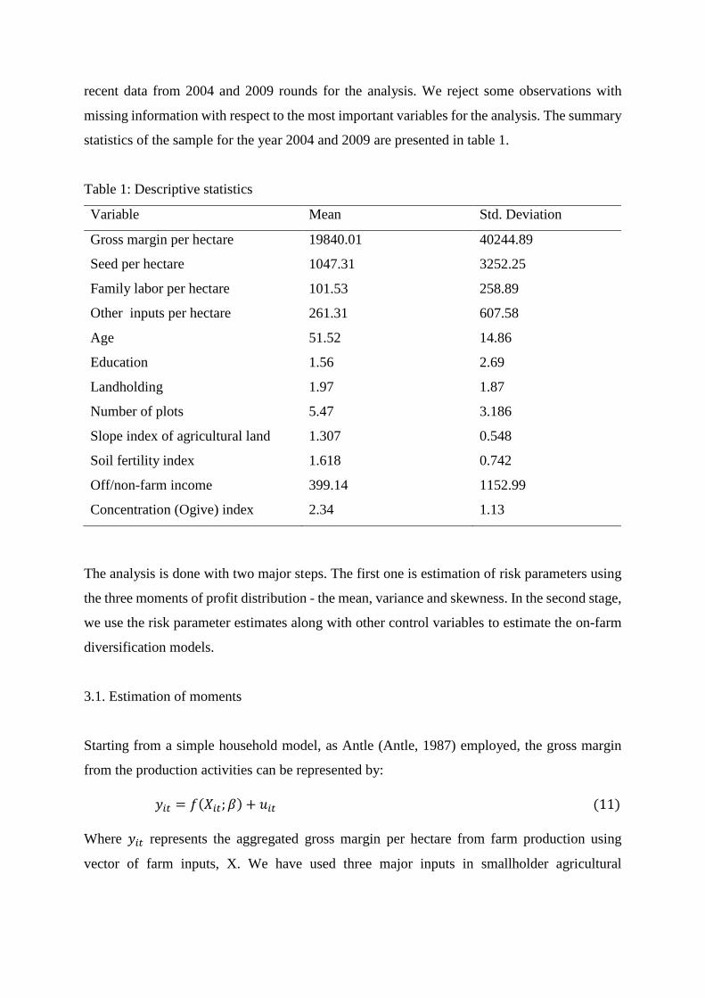
recent data from 2004 and 2009 rounds for the analysis. We reject some observations with
missing information with respect to the most important variables for the analysis. The summary
statistics of the sample for the year 2004 and 2009 are presented in table 1.
Table 1: Descriptive statistics
Variable Mean Std. Deviation
Gross margin per hectare 19840.01 40244.89
Seed per hectare 1047.31 3252.25
Family labor per hectare 101.53 258.89
Other inputs per hectare 261.31 607.58
Age 51.52 14.86
Education 1.56 2.69
Landholding 1.97 1.87
Number of plots 5.47 3.186
Slope index of agricultural land 1.307 0.548
Soil fertility index 1.618 0.742
Off/non-farm income 399.14 1152.99
Concentration (Ogive) index 2.34 1.13
The analysis is done with two major steps. The first one is estimation of risk parameters using
the three moments of profit distribution - the mean, variance and skewness. In the second stage,
we use the risk parameter estimates along with other control variables to estimate the on-farm
diversification models.
3.1. Estimation of moments
Starting from a simple household model, as Antle (Antle, 1987) employed, the gross margin
from the production activities can be represented by:
𝑦𝑖𝑡 = 𝑓(𝑋𝑖𝑡; 𝛽) + 𝑢𝑖𝑡 (11)
Where 𝑦𝑖𝑡 represents the aggregated gross margin per hectare from farm production using
vector of farm inputs, X. We have used three major inputs in smallholder agricultural

production. Seed cost, family labor and other intermediate inputs2 are aggregated per hectare of
land (Groom et al., 2008, Finger and Sauer, 2014). Following previous empirical works, for
example (Groom et al., 2008, Vollenweider et al., 2011), all the variables are rescaled with their
standard deviations.
One crucial step in the estimation procedure is to decide the functional form for the profit
function. The results of the overall procedure are influenced by the choice of the functional
form (Antle, 1983, Kumbhakar and Tveteras, 2003, Vollenweider et al., 2011). We have
employed a quadratic specification, which is commonly used in empirical papers (Antle, 1983,
Groom et al., 2008, Vollenweider et al., 2011, Zuo et al., 2014). Hence, the input levels, their
interaction terms and the square of the input levels are used as explanatory variables in this
function.
The basic premises in the moment based approach is to capture the risk attitude of the household
in the residual of the estimation (𝑢𝑖𝑡), which is assumed to have a zero mean and variance (δ2).
The residuals of equation (11) then used to estimate the second (variance) and third (skewness)
order moments of profit distribution. The square and cube of the residuals are regressed with
the same explanatory variables (inputs, input squares and the interaction terms) included in the
first moment (mean) estimation. Fixed effect model was used for the estimation of the first,
second and third order moments of profit distribution.
�̂�𝑖𝑡2 = 𝑔(𝑋𝑖𝑡; 𝛼) + �̌�𝑖𝑡 (12)
And
�̂�𝑖𝑡3 = ℎ(𝑋𝑖𝑡; 𝛾) + �̃�𝑖𝑡 (13)
These estimated coefficients (𝛽,̂ �̂�, and 𝛾) will then be used to compute the marginal
contribution of each input are computed. By recalling equation (6), we finally regress the
derivatives of variance and skewness functions over of the derivative of the expected profit
function with a 3SLS method. The region dummy, livestock holding and access to credit are
assumed exogenous to the risk attitude, while are correlated with the input use of farmers.
Hence, they can be used as instruments in the estimation procedure.
2 Intermediate inputs include fertilizer, pesticides and hired labor

Arrow-Pratt (AP) absolute risk aversion and downside (DS) risk aversion estimates can be
computed from this estimation (equation 7 and 8). In the estimation procedure, we didn’t
employ a constraint to keep the relative risk premium to be positive. However, like Groom et
al (Groom et al., 2008), those observations that are not following the assumption of risk
neutrality and risk aversion are neglected when calculating the average relative risk premium
for the population.
3.2. On-farm diversification and participation in off-farm activities
The second stage of the analysis estimates the implication of risk on smallholder farmer’s on-
farm diversification and participation of off-farm activities. The basic hypothesis is that
farmers’ decision to allocate their scarce resources is influenced by their risk perception and
experience. This has got special importance in Ethiopia where both production and market
related risks play a significant role (Dercon, 2004, Di Falco and Chavas, 2009, Mintewab and
Sarr, 2012). Household level adaptation mechanisms are crucial in these countries where the
institutional support mechanisms to mitigate risk are not well developed (Yesuf and Bluffstone,
2009, Hailemariam and Köhlin, 2011).
Following on previous empirical endogenous technology adoption models under risk (Kim and
Chavas, 2003, Mintewab and Sarr, 2012, Finger and Sauer, 2014, Zuo et al., 2014), we develop
a model for the adoption of on-farm diversification. In the literature of diversification, variety
of approaches have been employed to measure the diversification level of farm
households(Mintewab and Sarr, 2012, Finger and Sauer, 2014). We use Ogive index to measure
the level of diversification in the household farm portfolio. This approach was used to measure
the export diversification level by Ali et al (Ali et al., 1991) and on farm diversification by
Coelli and Fleming (Coelli and Fleming, 2004). The Ogive index is preferred from the count
index since it considers intensity of diversification of the production activities.
𝑂𝑔𝑖𝑣𝑒 = ∑(𝑋𝑛−(1
𝑁⁄ ))2
1𝑁⁄
𝑁𝑛=1 (14)
Where N is the total production activities and Xn is the share of the total land allocated for the
production activities (cereal crops, pulse crops, horticultural crops, tree and grass production).
This index measures deviation of the overall farm plan from equivalent allocation of land
among production activities.
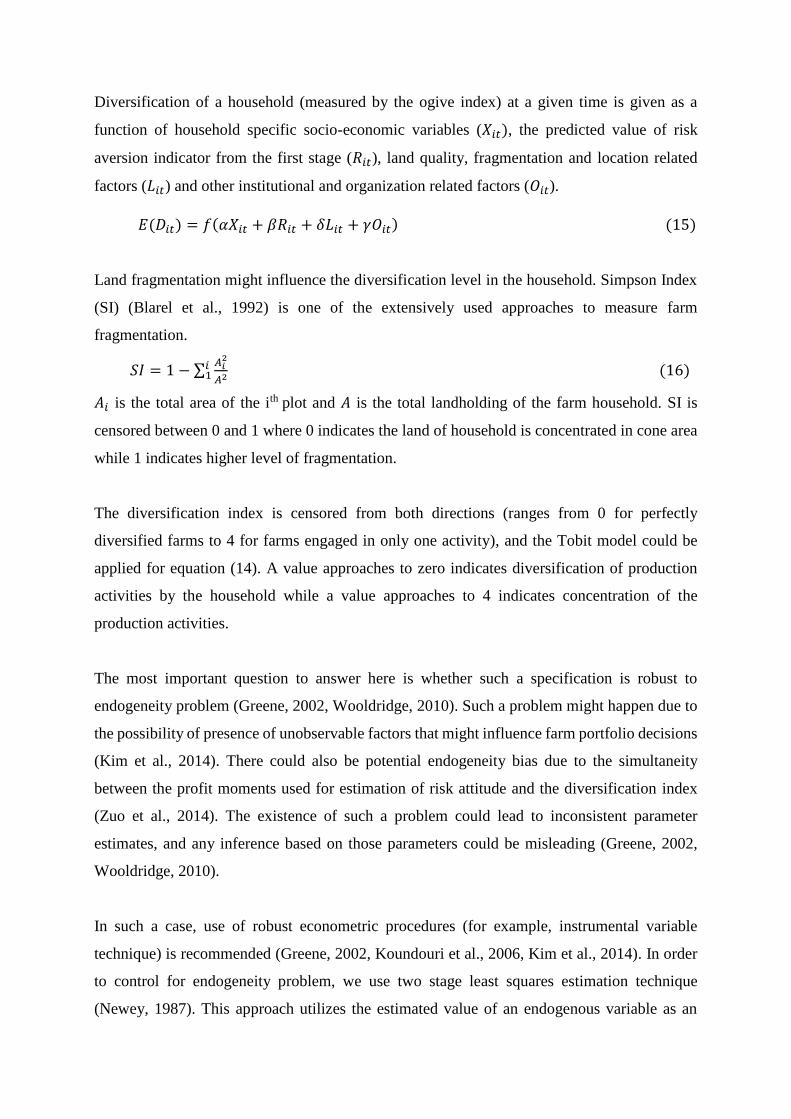
Diversification of a household (measured by the ogive index) at a given time is given as a
function of household specific socio-economic variables (𝑋𝑖𝑡), the predicted value of risk
aversion indicator from the first stage (𝑅𝑖𝑡), land quality, fragmentation and location related
factors (𝐿𝑖𝑡) and other institutional and organization related factors (𝑂𝑖𝑡).
𝐸(𝐷𝑖𝑡) = 𝑓(𝛼𝑋𝑖𝑡 + 𝛽𝑅𝑖𝑡 + 𝛿𝐿𝑖𝑡 + 𝛾𝑂𝑖𝑡) (15)
Land fragmentation might influence the diversification level in the household. Simpson Index
(SI) (Blarel et al., 1992) is one of the extensively used approaches to measure farm
fragmentation.
𝑆𝐼 = 1 − ∑𝐴𝑖
2
𝐴2𝑖1 (16)
𝐴𝑖 is the total area of the ith plot and 𝐴 is the total landholding of the farm household. SI is
censored between 0 and 1 where 0 indicates the land of household is concentrated in cone area
while 1 indicates higher level of fragmentation.
The diversification index is censored from both directions (ranges from 0 for perfectly
diversified farms to 4 for farms engaged in only one activity), and the Tobit model could be
applied for equation (14). A value approaches to zero indicates diversification of production
activities by the household while a value approaches to 4 indicates concentration of the
production activities.
The most important question to answer here is whether such a specification is robust to
endogeneity problem (Greene, 2002, Wooldridge, 2010). Such a problem might happen due to
the possibility of presence of unobservable factors that might influence farm portfolio decisions
(Kim et al., 2014). There could also be potential endogeneity bias due to the simultaneity
between the profit moments used for estimation of risk attitude and the diversification index
(Zuo et al., 2014). The existence of such a problem could lead to inconsistent parameter
estimates, and any inference based on those parameters could be misleading (Greene, 2002,
Wooldridge, 2010).
In such a case, use of robust econometric procedures (for example, instrumental variable
technique) is recommended (Greene, 2002, Koundouri et al., 2006, Kim et al., 2014). In order
to control for endogeneity problem, we use two stage least squares estimation technique
(Newey, 1987). This approach utilizes the estimated value of an endogenous variable as an

instrumental variable in two stage procedure(Greene, 2002, Wooldridge, 2010). In the first
stage, we regress the risk parameter with some explanatory variables3 which we assume to
influence the risk behavior of farm households. The estimated value of the risk parameter,
which is assumed exogenous, then will be used as explanatory variable in the diversification
model.
After the consideration of the instrumental variable, the two stage least square estimation looks
like:
𝐸(𝐷𝑖𝑡) = 𝑓(𝛼𝑋𝑖𝑡 + 𝛽𝑅𝑖�̂� + 𝛿𝐿𝑖𝑡 + 𝛾𝑂𝑖𝑡 + 𝜏𝑅𝑖(𝑡−1) + 𝜎𝑌𝑖(𝑡−1) + 𝜌𝐷𝑖(𝑡−1)) (17)
𝐸(𝑅𝑖�̂�) = 𝑓( 𝑅𝑖(𝑡−1), 𝑌𝑖(𝑡−1), 𝑋𝑖𝑡, 𝐿𝑖𝑡, 𝑂𝑖𝑡, 𝐴𝑖, )
We include lagged moments and the estimated risk parameter as explanatory variable in the
diversification model. Diversification could also be influenced by the previous experience in
diversification and the income levels in the preceding periods. In addition to their empirical
meanings, the lagged data inclusion in the model helps to control for some unobservable effects
(Wooldridge, 2010, Kim et al., 2014, Zuo et al., 2014).
4. Result and Discussions
4.1. Estimation of risk parameters
The main objective of the first stage estimation is to capture the risk attitude of farm households
from the profit moments. We estimate the profit function with the quadratic specification, which
is more flexible and commonly employed in empirical literatures (Groom et al., 2008,
Vollenweider et al., 2011, Finger and Sauer, 2014). Most covariates used in the estimation have
got the expected sign and the overall statistical significance of the estimated model is good. We
have also used the Feasible Generalized Least Squares (FGLS) estimation and the result is
similar to the one estimated with the fixed effect procedure. The Hauseman specification test
rejected the null hypothesis that the random and fixed effect model give similar results.
Accordingly, we use the fixed effects estimator for the profit moments estimation. The results
3 We use the lagged risk estimate and income of the household, household specific socio-economic variables, farm
land quality and fragmentation and organizational and institutional factors as instruments in the first stage.

of the fixed effect estimation of the first moment (mean), second moment (variance) and third
moment (skewness) are presented in table 2.
Table 2: Fixed effect estimates of first, second and third moments
Variables Gross margin �̂�𝑖𝑡2 �̂�𝑖𝑡3
Coeff. Std.err Coeff. Std.err Coeff. Std.err
Seed -0.391*** 0.070 -1.330*** 0.389 -8.163*** 2.979
Family labor 0.158*** 0.054 0.739*** 0.301 5.783** 2.299
Other inputs 0.264*** 0.064 0.864*** 0.351 6.045** 2.689
Seedsq. 0.053*** 0.010 0.173*** 0.057 0.944** 0.440
laborsq -0.021*** 0.004 -0.061*** 0.023 -0.557*** 0.177
Otherinpsq. -0.007 0.006 -0.066* 0.037 -0.614** 0.287
Seed*labor 0.029*** 0.008 -0.031 0.045 -0.121 0.345
Seed*other -0.051*** 0.012 -0.064 0.069 -0.233 0.535
Labor*other 0.245*** 0.007 0.074* 0.041 0.764** 0.312
Year dummy 0.297*** 0.045 1.169*** 0.251 7.398*** 1.921
Const. 0.178*** 0.028 0.355** 0.157 1.011 1.199
Hauseman test (Chi2) 147.66 *** 133.02*** 101.90***
N of households =2724 * if p < 0.10, ** if p < 0.05, *** if p < 0.01
We use the estimation in table 2 to estimate the marginal effects of each input for each
individual observation. Following this procedure, we estimate the first order condition
described in equation 6 using three stage least squares (3SLS) procedure. We have also
employed Seemingly Unrelated Regression approach for the first order condition for
consistency reasons are the result remains the same. The coefficients of these functions are used
to estimate the Arow-Pratt absolute risk aversion (AP) and downside risk aversion (DS) which
then will be used to estimate the relative risk premium (RRP).
Table 3: Risk parameters
Inputs Seed Family labor Other inputs
Coeff. Std. err Coeff. Std. err Coeff. Std. err
Constant 0.008 0.005 0.125*** 0.002 -0.023*** 0.002
𝜃2 0.685*** 0.024 -1.263*** 0.016 0.849*** 0.008

𝜃3 -0.063*** 0.004 0.167*** 0.002 -0.074*** 0.000
AP 1.37 -2.52 1.69
DS 0.38 -1.00 0.44
RRP 25.7% 12.2% 16.9%
Chi2 test of parameters
equality
23533.49 24740.17 12493.40
p> x2=0.0000 p> x2=0.0000 p> x2=0.0000
N of households= 2688 * p < 0.10, ** p < 0.05, *** p < 0.01
Estimation: 3SLS with region dummy, access to credit and livestock ownership in TLU as
instruments
The Wald test of parameters equality was employed for the three estimations and rejected the
null hypothesis of parameters equality between inputs. Except for the family labor, farmers
show risk aversion behavior with respect to the other two inputs used in the production process.
They exhibit risk averse behavior in terms of both absolute risk aversion (variability of returns)
and downside risk aversion (e.g. risks related to crop failure, bad harvest or price fall). Farmers
are willing to cost some of their profit to avoid risk related to seed and other intermediate inputs.
The coefficients in the estimation of FOC for family labor come up with an interesting result.
The negative values in the AD and DS indicates that farmers seem risk loving with respect to
family labor. This could be due to the limited off-farm and non-farm employment opportunities
on the one hand and low level of wage rate for the available ones in rural Ethiopia. Most farms
in rural Ethiopia use family labor for the production activities and sometimes use hired labor in
peak seasons. Given the low level of opportunity cost they experience in family labor, they
would likely choose to employ the available labor though remained risky.
We find that an average sample relative risk premium of 18.27%4, with the overall picture in
line with previous studies. The rough estimate for the willingness to pay of farmers in order to
avoid risk is 3864 Birr. Most of the previous studies are done in developed or transition
economies where the insurance and other risk mitigation mechanisms are relatively developed.
Hence, the relative risk premium of farmers in developing countries with underdeveloped
4 When calculating the sample relative risk premium, the observations with negative RRP has been neglected since
they are not in line with the assumptions of risk aversion and risk neutrality (for further information, see Groom
et al, 2008).

insurance and risk mitigation schemes is expected to be higher than those in the developed and
transition economies. Given the higher level of unemployment condition and the low wage rate
condition of the available options, the difference in the risk behavior related to family labor
used is expected. Groom et al (Groom et al., 2008) in Cyprus have found the RRP ranging from
6% to 20% with respect to different inputs. They indicated that the RRP is different among
producers of different types of crops. Vollenweider et al (Vollenweider et al., 2011) and
Kumbhakar and Tveteras (Kumbhakar and Tveteras, 2003) have got RRP estimate of 16% and
18% in Irish Dairy sector and Norwegian salmon famers respectively.
4.2. Role of risk behavior on farm portfolio
The research hypothesis of the study is whether farmers opt to diversify their farm activities in
order to mitigate risk. The overall model adequacy of the two-step Tobit model with
endogenous regressors is good and the results of the model are illustrated in table 4. The Wald
test of exogeneity rejects the null hypothesis of no endogeneity and hence, our use of the two
stage least squares estimation technique is justified.
Table 4: Estimation of two step Tobit (dep. Var. = diversification)
Variables Coeff. Std. err T
Relative Risk Premium (RRP) -0.620** 0.282 -2.20
Relative Risk Premium lagged (t-1) -0.014 0.022 -0.64
Concentration index lagged (t-1) 0.202*** 0.038 5.30
Income lagged (t-1) -0.003 0.009 -0.28
Age -0.001 0.003 -0.45
Education level -0.027* 0.016 -1.68
Landholding 0.027 0.028 0.96
Land fragmentation (Simpson index) -1.003*** 0.224 -4.47
Slope index of land 0.142 0.092 1.54
Soil fertility index -0.018 0.075 -0.24
Slope*fertility -0.013 0.014 -0.92
Off/non-farm income 0.006* 0.003 1.94
Access to credit -0.200** 0.087 -2.30
Extension contact (frequency) 0.010 0.016 0.62

Regional dummy_Amhara 0.383** 0.188 2.03
- Oromiya 1.069*** 0.219 4.88
- South -0.294* 0.175 -1.68
Constant 2.471*** 0.378 6.53
Number of observations= 947 * p < 0.10, ** p < 0.05, *** p < 0.01
Model: Two-step least squares Tobit model with endogenous regressors5
Model adequacy: Wald-chi2 (17)=247.3 prob>chi2=0.0000
Wald test of exogeneity chi2 = 5.32 Prob > chi2 = 0.021
Regional dummy is found significant in our estimation. Different regions could have different
physical, agro-ecological and bio-diversity, socio-economic and institutional conditions. In
addition to the above mentioned features, the level of risk and the associated risk parameters
are different across regions. The diversification level of farms is different in different regions
of the country. Some of the variability in diversification level of farms across regions is related
to the existing physical, agro-ecological, climatic, and socio-economic situations. The
production structure, occurrence of climate extremes and the organizational structure of markets
is quite different in those regions, and this in turn might have an implication for risk aversion
behavior of farm households. These concepts will further be explained in detail with the
following paragraphs.
Education level of the household negatively influences the concentration index. People with
better education are more likely to opt for more diversified farms. The benefits of diversification
might outweigh to the benefits of concentrated farms in smallholder agriculture (Coelli and
Fleming, 2004). Farmers with better education could likely adjust their farm portfolio easily as
compared to the illiterate counterparts. Mintwab and Sarr (Mintewab and Sarr, 2012) have also
found education level of household head positively associated with the on-farm diversification
level.
The coefficient of the lagged concentration index is positive and significant. Finger and Sauer
(Finger and Sauer, 2014) have got similar findings. Concentration level of farms is influenced
by past experience in concentration. The important feature of panel data format is the ability of
5 We use livestock ownership, frequency of extension contact and income of the previous period as instruments

inclusion of lagged variables to explain some of the variability. This otherwise could happen to
be explained by other covariates in a cross-sectional data types.
Households’ access to credit is negatively associated with concentration index of farms. In
smallholder agriculture, where farmers are frequently facing liquidity related constraints, access
to credit might influence the farm portfolio related decisions. Households will have more
flexibility in allocating resources to different production schemes based on their liquidity
conditions.
Land fragmentation influences the land allocation decision of farm households. The more the
land is spatially fragmented, farmers are likely to diversify their production activities. It in fact
matters if there is a difference in the suitability of the farm plots6 for different production
activities. There might also be a tradeoffs in labor and other production inputs among the
production activities. Accessibility of the plots for routine farm management, supervision or
transportation are also essential in the decision making process. Benin et al (Benin et al., 2003)
find out contradicting results of diversity across different slope levels and access to irrigation
water.
Off-farm/ non-farm income is negatively associated with the on-farm diversification level of
the household. This is in line with previous researches on the trade-off between on-farm
diversification and off-farm income (Woldehana et al., 2000, Serra et al., 2005, Finger and
Sauer, 2014). Finger and Sauer (Finger and Sauer, 2014), for example, argue that farmers might
choose either to diversify their farm or look for off-farm investment options as a response to
occurrence of extreme events. They highlighted that farms may prefer to stay specialized,
though risky. Such farms might involve in off-farm activities to mitigate risk of extreme events.
Based on our finding, we could argue that farmers might use their off-farm income to invest in
a more specialized farm portfolio with higher expected profit. They might prefer to specialize
and use the off-farm income as a safety net in case of extreme events. There could also a
possibility for competition of labor among these two and engagement in off-farm and non-farm
income and on farm diversification could be seen as substituting strategies when it comes to
agricultural risk mitigation.
6 As we include fertility and slope index of the plots in the estimation procedure, it is vital to note that the influence
from land fragmentation is not related to these variables.

We verified the research hypothesis of the paper and relative risk premium is positively
associated with on-farm diversification. The lagged relative risk premium has also got the
expected sign, though remained insignificant. Given the long gap between the two time frames
in the panel data, these estimation is fairly good. This is in line with both the theoretical
literatures in applied economics and empirical works. Mintwab and Sarr (Mintewab and Sarr,
2012) have found similar result using the application of experimental risk elicitation technique.
Finger and Sauer (Finger and Sauer, 2014) have got an evidence on the association of lagged
flood occurrence and the level of diversification.
5. Conclusion and Policy Implications
We have used the panel data of households in Ethiopia to develop an empirical model to analyze
the implication of farmers risk behavior on their farm decision making. This work adds up to
the existing literature with the application of a more extensive in terms of exploiting the
household, farm and regional level information and robust approach in its econometric
specification. We try to capture on-farm diversification decision of the households using a more
recent and robust risk elicitation econometric approaches from profit moments. In addition, we
make use of panel data which allows us to capture both the within and between variation in the
estimation of risk premium.
We have estimated the relative risk premium (18.27%) which is in line with most of the previous
findings. The sample average willingness to pay for risk aversion is estimates around 3864 Birr.
This can be translated as a rough estimate of farmer’s willingness to pay for risk (such as income
variability, crop failure, price fall, forward contracts and future markets etc.). There are some
initiations from the government and some organizations towards index based insurance
schemes in the country. There is also an interest to initiate future markets integrated with the
commodity exchange in Ethiopia. This finding could helpful to develop strategies and policies
to implement such insurance schemes and integrate smallholder farmers to the future markets
in the country.
Household head’s education level, and access to credit influence the level of on-farm
diversification. Risk behavior is positively associated to on-farm diversification and farmers
with a higher level of relative risk premium are more likely to opt for diversification of farms.
The engagement of farm households to off and non-farm income generating activities could

reduce the incentive to diversify in the farm level. The income generated could improve the
liquidity condition of the farm and such farms might choose specialized commercial orientation.
These could be due to the fact that households with extra income from off and non-farm
activities use this income as a safety net and go for concentrated farms. Hence, from the risk
perspective, there two can be considered as substitutable risk mitigation strategies.
6. References
ALEM, Y., MINTEWAB, B., MINALE, K. & ZIKHALI, P. 2010. Does Fertilizer Use Respond to
Rainfall Variability? Panel Data Evidence from Ethiopia. Agricultural Economics, 41, 165-175.
ALI, R., ALWANG, J. & SIEGEL, P. B. 1991. Is Export Diversification the Best Way to Achieve
Export Growth and Stability? A Look at Three African Countries. Working Papers Series
Washington, D.C.: Policy, Research and External Affairs, Agriculture Operations, World Bank,.
ANTLE, J. M. 1983. Testing the Stochastic Structure of Production: A Flexible Moment-Based
Approach. Journal of Business and Economic Statistics, 1, 192-201.
ANTLE, J. M. 1987. Econometric Estimation of Producers’ Risk Attitudes. American Journal of
Agricultural Economics, 69, 509-522.
ARROW, K. J. 1965. Aspects of the Theory of Risk Bearing, Helsinki, Finland, Yrjo Jahnsson Saatio.
BENIN, S., SMALE, M., GEBREMEDHIN, B., PENDER, J. & EHUI, S. 2003. The Determinants of
Cereal Crop Diversity on Farms in the Ethiopian Highlands. 25th International Conference of
Agricultural Economists. Durban, South Africa.
BLAREL, B., HAZZEL, P., PLACE, F. & QUIGGIN, J. 1992. The Economics of Farm Fragmentation:
Evidence from Ghana and Rwanda. World Bank Economic Review, 6, 233-354.
BOZZOLA, M. 2014. Adaptation to Climate Change: Farmers' Risk Preferences and the Role of
Irrigation. European Association of Agricultural Economists Conference on 'Agri-Food and
Rural Innovations for Healthier Societies. Ljubljana, Slovenia.
CHAVAS, J. P. 2004. Risk Analysis in Theory and Practice, San Diego, Elsevier.
CHAVAS, J. P., CHAMBERS, R. G. & POPE, R. D. 2010. Production Economics and Farm
Management: A Century of Contributions. American Journal of Agricultural Economics, 92,
356-375.
COELLI, T. & FLEMING, E. 2004. Diversification Economies and Specialization Efficiencies in a
Mixed Food and Coffee Smallholder Farming System in Papua New Guinea. Agricultural
Economics, 31, 229-239.
DERCON, S. 2004. Growth and shocks: evidence from rural Ethiopia. Journal of Development
Economics, 74, 309–329.
DI FALCO, S. & BULTE, E. 2013. The Impact of Kinship Networks on the Adoption of Risk-Mitigating
Strategies in Ethiopia. World Development 43, 100-110.
DI FALCO, S. & CHAVAS, J. P. 2009. On Crop Biodiversity, Risk Expossure and Food Security in the
Highlands of Ethiopia. American Journal of Agricultural Economics 91, 599-611.
FINGER, R. & SAUER, J. 2014. Climate Risk Management Strategies in Agriculture-The Case of Flood
Risk. Agricultural and Applied Economics Association Annual Meeting. Minneapolis, USA.
FRANKLIN, S., MDUMA, J., PHIRI, A., THOMAS, A. & ZELLER, M. 2006. Can Risk-Aversion
Toward Fertilizer Explain Part of the Non-Adoption Puzzle for Hybrid Maize? Empirical
Evidence from Malawi. Journal of Applied Sciences, 6, 1490-1498.
GREENE, W. H. 2002. Econometric Analysis, Upper Saddle River, New Jersey, Pearson Education,
Inc.
GROOM, B., KOUNDOURI, P., NAUGES, C. & THOMAS, A. 2008. The Story of the Moment: Risk
Averse Cypriot Farmers Respond to Drought Management. Applied Economics 40, 315-326.
HAILEMARIAM, T. & KÖHLIN, G. 2011. Risk Preferences as Determinants of Soil Conservation
Decisions in Ethiopia. Journal of Soil and Water Conservation, 66, 87-96.
HARDAKER, J. B., HUIRNE, R. M. B., ANDERSON, J. R. & LIEN, G. 2004. Coping with Risk in
Agriculture, Wallingford, CAB International
IPCC 2007. Summary for policymakers. Climate change 2007: The physical science basis. Working
group I contribution to IPCC fourth assessment report. Geneva, Switzeland.
KIM, K. & CHAVAS, J. P. 2003. Technological Change and Risk Management: An Application to the
Economics of Corn Production. Agricultural Economics, 29, 125-142.
KIM, K., CHAVAS, J. P., BARHAM, B. & FOLTZ, J. 2014. Rice, Irrigation and Downside Risk: A
Quantile Analysis of Risk Exposure and Mitigation on Korean Farms. european Review of
Agricultural Economics, 41, 775-815.
KIMBALL, M. S. 1990. Precautionary Saving in the Small and in the Large. Econometrica, 58, 53-73.
KOUNDOURI, P., NAUGES, C. & TZOUVELEKAS, V. 2006. Technology Adoption under
Production Uncertainty: Theory and Application to Irrigation Technology. American Journal of
Agricultural Economics, 88, 657-670.
KUMBHAKAR, S. C. & TVETERAS, R. 2003. Risk Preferences, Production Risk and Firm
Heterogeneity. The Scandinavian Journal of Economics, 105, 275-293.
LIVINGSTON, M. J. & MISHRA, A. K. 2013. Risk Attitudes and Premiums of U.S. Corn and Soybean
Producers: An Empirical Investigation. Empirical Economics, 44, 1337-1351.
MENEZES, C., GEISS, C. & TRESSLER, J. 1908. Increasing Down-Side Risk. American Economic
Review, 70, 921-932.
MINTEWAB, B. & SARR, M. 2012. Risk Preferences and Environmental Uncertainty: Implications
for Crop Diversification Decisions in Ethiopia. Environmental and Resource Economics, 53,
483-505.
NEWEY, W. K. 1987. Efficient Estimation of Limited Dependent Variable Models with Endogenous
Explanatory Variables. Journal of Econometrics, 36, 231–250.
NIELSEN, T., KEIL, A. & ZELLER, Z. 2013. Assessing Farmers’ Risk Preferences and their
Determinants in a Marginal Upland area of Vietnam: A Comparison of Multiple Elicitation
Techniques. Agricultural Economics, 44, 255–273.
OREA, L. & WALL, A. 2012. Productivity and Producer Welfare in the Presence of Production Risk.
Journal of Agricultural Economics, 63, 102-118.
PRATT, J. W. 1964. Risk Aversion in the Small and in the Large. Econometrica 32, 122-136.
SAUER, J. 2011. Natural Disasters and Agriculture: Individual Risk Preferences towards Flooding.
Vortrag anlässlich der 51. Jahrestagung der GEWISOLA. Halle, Germany.
SERRA, T., GOODWIN, B. K. & FEATHERSTONE, A. M. 2005. Agricultural Policy Reform and Off-
farm Labor Decisions. Journal of Agricultural Economics, 56, 271-285.
TAYLOR, C. R. 1984. A Flexible Method for Empirically Estimating Probability Functions. Western
Journal of Agricultural Economics, 9, 66-75.
TEGEGNE, G. & HOLDEN, S. T. 2011. Distress Rentals and the Land Rental Market as a Safety Net:
Contract Choice Evidence from Tigray, Ethiopia. Agricultural Economics, 42, 45-60.
VOLLENWEIDER, X., DI FALCO, S. & O'DONOGHUE, C. 2011. Risk Preferences and Voluntary
Agri-environmental Scemes: Does Risk Aversion Explainthe Uptake of the Rural Environment
Protection Scheme? EAAE Congress. Zurich, Switzerland.
WOLDEHANA, T., LANSINK, A. O. & PEERLINGS, J. 2000. Off-farm Work Decisions on Dutch
Cash Crop Farms and the 1992 and Agenda 2000 CAP Reforms. Agricultural Economics, 22,
163-171.
WOOLDRIDGE, J. M. 2010. Econometric Analysis of Cross Section and Panel Data, Cambridge, MA,
MIT Press.
YESUF, M. & BLUFFSTONE, R. A. 2009. Poverty, risk aversion and path dependence in low-income
countries: Experimental evidence from Ethiopia. American Journal of Agricultural Economics,
91, 1022-1037.
ZUO, A., NAUGES, C. & SARAH, A. W. 2014. Farmers' Exposure to Risk and their Temporary Water
Trading. European Review of Agricultural Economics, 41, 1-24.


