
OPTIMIZING THE PERFORMACE OF ACHIP SHOOTER MACHINE
Fernando J. Vittes
Thesis submitted to the Faculty of theVirginia Polytechnic Institute and State University
in partial fulfillment of the requirements for the degree of
Master of ScienceIn
Industrial and Systems Engineering
Kimberly P. Ellis, ChairJohn Kobza
William G. Sullivan
August 12, 1999Blacksburg, Virginia
Keywords: Surface Mount, Component Placement Sequence, Feeder Assignment
Copyright 1999, Fernando J. Vittes

ii
OPTIMIZING THE PERFORMACE OF A
CHIP SHOOTER MACHINE
Fernando J. Vittes
(ABSTRACT)
Process planning is an important and integral part of operating a printed circuit board (PCB)
assembly system effectively. The focus of this research is to develop a new solution approach to
determine the component placement sequence and feeder assignment for a turret style Chip
Shooter machine often used in PCB assembly systems. This solution approach can be integrated
into a process planning system to reduce assembly time and improve productivity.
The Chip Shooter machine consists of three primary mechanisms: the turret head, a moving
table, and the feeder carriage. These mechanisms move simultaneously in a cyclic manner to
mount the components on the PCB. The mechanism with the longest movement time determines
the placement time of a component. Therefore, the placement sequence of the components and
the arrangement of the feeders in the feeder carriage directly affect the time required to mount all
the components on a PCB. A placement time estimator function that accounts for the functional
characteristic of the Chip Shooter machine is developed and is used to evaluate the performance
of the solution approach presented in this research.
The solution approach consists of a construction algorithm that uses a set of knowledge-based
rules to construct an initial placement sequence and feeder assignment, and an improvement
procedure to improve the initial solution. A case study is presented to validate the proposed
solution approach. A Fuji CP4-3 machine and actual PCB data are used to test the performance
of the proposed solution approach for different machine setup scenarios. The solutions obtained
using the proposed solution approach are compared to those obtained using state of the art PCB
assembly process optimization software. For all PCBs in the case study, the proposed solution
approach yielded lower placement times than the commercial software, thus generating
additional valuable production capacity.

iii
ACKNOWLEDGEMENTS
Many people have contributed to the completion of this thesis. I appreciate the support I have
received from professors, friends, industrial partners, and family while conducting this research.
Dr. Kimberly Ellis and Dr. John Kobza have served as my research academic advisors
throughout my graduate studies at Virginia Tech. They invited me to join them in several
collaborative projects with Ericsson, Inc., which eventually lead to this research. I would like to
thank my advisor, Dr. Kimberly Ellis, and committee member, Dr. John Kobza for their advice,
support and encouragement throughout my graduate studies. I also like to thank my advisor for
her patience and time in correcting and re-correcting this thesis to give it the proper professional
form and for teaching me much of what I know about process planning in printed circuit board
assembly systems. I would also like to thank Dr. William Sullivan for participating on my
committee and for his helpful suggestions on the proposal.
The full financial support received through this collaborative project with Ericsson, Inc. is
gratefully acknowledged. I would also like to thank Mr. Larry Hatch, Mr. Anders Sjolund, Mr.
Brian Barley, and Johan Malmros from Ericsson, Inc. for their support, time, and collaboration
and for providing me with the necessary data to complete this research.
I would also like to thank Bob Noble from the Virginia Tech Statistical Consulting Center, for
his advice on conducting and analyzing the experiments included in this research.
I want to extend my gratitude to my special friends from Blacksburg for their moral support. My
heart will always be with you.
Furthermore I want to express my love to my parents, Ana Maria and Pedro for their love and
support through the years. I also appreciate the trust and support shown by my brothers, Carlos,
Jorge, Mario, and Pedro, and my girlfriend, Melitza.
Last, but not least, I want to thank God.

iv
TABLE OF CONTENTS
ABSTRACT ......................................................................................................... ii
ACKNOWLEDGEMENTS ................................................................................ iii
LIST OF TABLES............................................................................................... vi
LIST OF FIGURES............................................................................................. x
LIST OF NOTATION......................................................................................... xi
CHAPTER
I. INTRODUCTION ................................................................................... 1
1.1 Overview of Electronic Assembly ............................................... 1
1.2 Motivation of Research................................................................ 2
1.3 Assembly Process and Machine Description ............................... 4
1.4 Organization of Thesis................................................................. 9
II. PROBLEM DESCRIPTION................................................................... 10
2.1 Problem Overview ...................................................................... 10
2.2 Statement of the Problem............................................................. 11
2.3 Research Strategy for Addressing Problem.................................. 11
III. LITERATURE SURVEY........................................................................ 13
3.1 Placement Sequencing................................................................. 13
3.2 Feeder Assignment ...................................................................... 19
3.3 Placement Sequencing and Feeder Assignment ........................... 22
3.4 Summary of Literature Review.................................................... 27
IV. ESTIMATOR FUNCTION FOR COMPONENT
PLACEMENT TIME .............................................................................. 29
4.1 Detailed Chip Shooter Machine Description................................ 29
4.2 Development of Placement Time Estimator Function.................. 33
4.3 Calculation of Experimental Placement Velocity Functions........ 38
4.3.1 Calculation of Minimum Turret Rotation Time and
Fixed Pick and Place Time................................................. 39
4.3.2 Calculation of PCB Table Average Velocity
Functions............................................................................ 41

v
4.3.3 Calculation of Feeder Carriage Average Velocity
Function ............................................................................. 49
4.4 Overall Placement Time Estimator Function ............................... 52
4.5 Validation of the CP4-3 Placement Time Estimator Function ..... 54
V. SOLUTION APPROACH AND OPTIMIZATION
CONSTRAINTS ...................................................................................... 58
5.1 General Optimization Solution Approach.................................... 58
5.2 Fixed Setup Optimization Solution Approach ............................. 64
5.3 Calculation of Lower Bound........................................................ 69
VI. CASE STUDY.......................................................................................... 74
6.1 Free Setup Case Study Results .................................................... 77
6.2 Fixed Setup Case Study Results................................................... 81
6.3 Partial Fixed Setup Case Study Results ....................................... 84
6.4 Summary of Case Study Results.................................................. 89
VII. RESULTS AND CONCLUSIONS.......................................................... 91
7.1 Conclusions ................................................................................. 91
7.2 Areas of Further Research ........................................................... 93
REFERENCES .................................................................................................... 96
APPENDIX A – GENERAL OPTIMIZATION SOLUTION
APPROACH EXAMPLE........................................................ 100
APPENDIX B – FIXED SETUP OPTIMIZATION SOLUTION
APPROACH EXAMPLE........................................................ 119
APPENDIX C – CASE STUDY DATA AND RESULTS ................................. 143
VITA..................................................................................................................... 209
vi
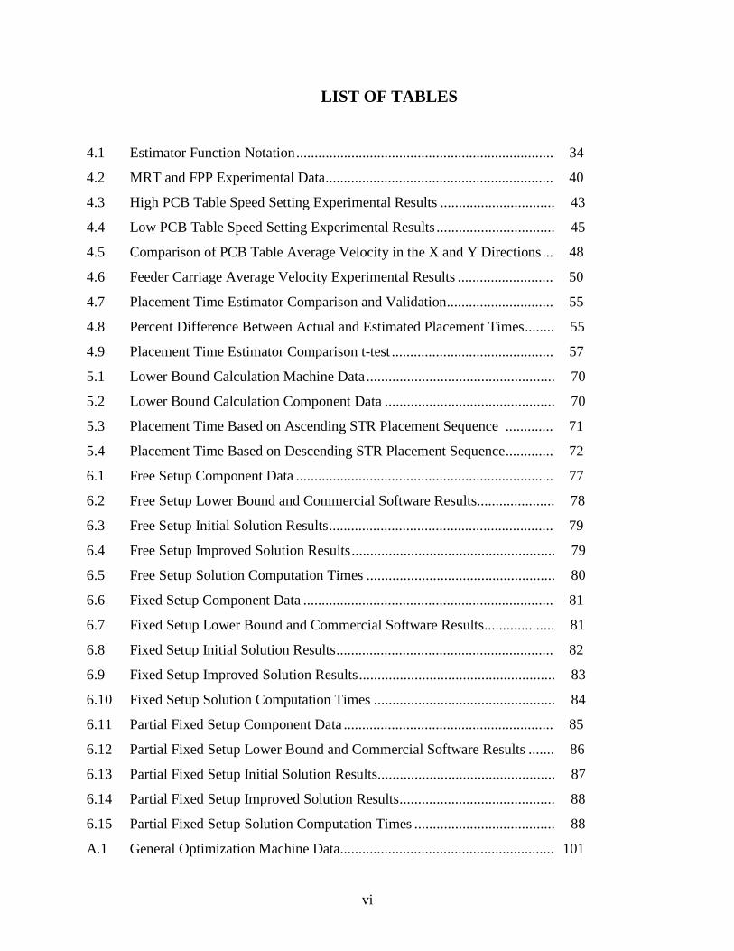
LIST OF TABLES
4.1 Estimator Function Notation...................................................................... 34
4.2 MRT and FPP Experimental Data.............................................................. 40
4.3 High PCB Table Speed Setting Experimental Results ............................... 43
4.4 Low PCB Table Speed Setting Experimental Results ................................ 45
4.5 Comparison of PCB Table Average Velocity in the X and Y Directions... 48
4.6 Feeder Carriage Average Velocity Experimental Results .......................... 50
4.7 Placement Time Estimator Comparison and Validation............................. 55
4.8 Percent Difference Between Actual and Estimated Placement Times........ 55
4.9 Placement Time Estimator Comparison t-test ............................................ 57
5.1 Lower Bound Calculation Machine Data................................................... 70
5.2 Lower Bound Calculation Component Data .............................................. 70
5.3 Placement Time Based on Ascending STR Placement Sequence ............. 71
5.4 Placement Time Based on Descending STR Placement Sequence............. 72
6.1 Free Setup Component Data ...................................................................... 77
6.2 Free Setup Lower Bound and Commercial Software Results..................... 78
6.3 Free Setup Initial Solution Results............................................................. 79
6.4 Free Setup Improved Solution Results....................................................... 79
6.5 Free Setup Solution Computation Times ................................................... 80
6.6 Fixed Setup Component Data .................................................................... 81
6.7 Fixed Setup Lower Bound and Commercial Software Results................... 81
6.8 Fixed Setup Initial Solution Results........................................................... 82
6.9 Fixed Setup Improved Solution Results..................................................... 83
6.10 Fixed Setup Solution Computation Times ................................................. 84
6.11 Partial Fixed Setup Component Data ......................................................... 85
6.12 Partial Fixed Setup Lower Bound and Commercial Software Results ....... 86
6.13 Partial Fixed Setup Initial Solution Results................................................ 87
6.14 Partial Fixed Setup Improved Solution Results.......................................... 88
6.15 Partial Fixed Setup Solution Computation Times ...................................... 88
A.1 General Optimization Machine Data.......................................................... 101

vii
A.2 General Optimization PCB Component Data............................................. 101
A.3 General Optimization Group 1 PCB Table Movement Time Matrix.......... 102
A.4 General Optimization Group Placement Sequences................................... 103
A.5 General Optimization Group 1 Component Type Flow Matrix.................. 104
A.6 General Optimization Group 2 Component Type Flow Matrix.................. 104
A.7 General Optimization Group 3 Component Type Flow Matrix.................. 104
A.8 General Optimization Group 4 Component Type Flow Matrix.................. 104
A.9 General Optimization Group Feeder Sequences......................................... 105
A.10 General Optimization Initial Feeder Assignment ....................................... 106
A.11 General Optimization Mtij Matrix ............................................................. 109
A.12 General Optimization Initial Solution Using N.N. Algorithm.................... 111
A.13 General Optimization Initial Solution Using A.I.P. Algorithm .................. 115
A.14 General Optimization Improved Placement Sequence Solution................. 117
A.15 General Optimization Improved Feeder Assignment Solution................... 118
B.1 Fixed Setup Optimization Machine Data Example .................................... 120
B.2 Fixed Setup Optimization Component Data Example................................ 120
B.3 Fixed Setup Component Data .................................................................... 121
B.4 Fixed Setup Optimization Initial Feeder Carriage Status ........................... 121
B.5 Fixed Setup Optimization Group 1 PCB Table Movement
Time Matrix............................................................................................... 122
B.6 Fixed Setup Optimization Group Placement Sequences ............................ 122
B.7 Fixed Setup Optimization Group 1 Component Type Flow Matrix ........... 123
B.8 Fixed Setup Optimization Group 2 Component Type Flow Matrix ........... 123
B.9 Fixed Setup Optimization Group 3 Component Type Flow Matrix ........... 124
B.10 Fixed Setup Optimization Group 4 Component Type Flow Matrix ........... 124
B.11 Fixed Setup Optimization Group 1 Updated Component Type Flow
Matrix 1 ..................................................................................................... 127
B.12 Fixed Setup Optimization Updated Feeder Carriage Status 1 .................... 127
B.13 Fixed Setup Optimization Group 1 Updated Component Type Flow
Matrix 2 ..................................................................................................... 127

viii
B.14 Fixed Setup Optimization Group 1 Updated Component Type Flow
Matrix 3 ..................................................................................................... 128
B.15 Fixed Setup Optimization Updated Feeder Carriage Status 2 .................... 128
B.16 Fixed Setup Optimization Group 2 Updated Component Type Flow
Matrix 1 ..................................................................................................... 129
B.17 Fixed Setup Optimization Updated Feeder Carriage Status 3 .................... 129
B.18 Fixed Setup Optimization Group 2 Updated Component Type Flow
Matrix 2 ..................................................................................................... 129
B.19 Fixed Setup Optimization Updated Feeder Carriage Status 4 .................... 130
B.20 Fixed Setup Optimization Updated Feeder Carriage Status 5 .................... 130
B.21 Fixed Setup Optimization Initial Feeder Assignment................................. 131
B.22 Fixed Setup Optimization Mtij Matrix....................................................... 133
B.23 Fixed Setup Optimization Initial Solution Using N.N. Algorithm ............. 135
B.24 Fixed Setup Optimization Initial Solution Using A.I.P. Algorithm............ 138
B.25 Fixed Setup Optimization Improved Placement Sequence......................... 140
C.1 PCB 1 Component Type Data.................................................................... 144
C.2 PCB 1 Component Location Data.............................................................. 145
C.3 PCB 1 Commercial Software Component Placement Sequence ................ 149
C.4 PCB 1 Commercial Software Feeder Assignment...................................... 153
C.5 PCB 1 A.I.P. Algorithm Initial Component Placement Sequence.............. 154
C.6 PCB 1 A.I.P. Algorithm Initial Feeder Assignment ................................... 158
C.7 PCB 1 A.I.P. Algorithm Improved Component Placement Sequence........ 159
C.8 PCB 1 A.I.P. Algorithm Improved Feeder Assignment ............................. 163
C.9 PCB 1 N.N. Algorithm Initial Component Placement Sequence................ 164
C.10 PCB 1 N.N. Algorithm Initial Feeder Assignment..................................... 168
C.11 PCB 1 N.N. Algorithm Improved Component Placement Sequence.......... 169
C.12 PCB 1 N.N. Algorithm Improved Feeder Assignment............................... 173
C.13 PCB 5 Component Type Data.................................................................... 174
C.14 PCB 5 Component Location Data.............................................................. 178
C.15 PCB 5 Commercial Software Component Placement Sequence ................ 180
C.16 PCB 5 Commercial Software Feeder Assignment...................................... 182

ix
C.17 PCB 5 A.I.P. Algorithm Initial Component Placement Sequence.............. 183
C.18 PCB 5 A.I.P. Algorithm Initial Feeder Assignment ................................... 185
C.19 PCB 5 A.I.P. Algorithm Improved Component Placement Sequence........ 186
C.20 PCB 5 A.I.P. Algorithm Improved Feeder Assignment ............................. 188
C.21 PCB 5 N.N. Algorithm Initial Component Placement Sequence................ 189
C.22 PCB 5 N.N. Algorithm Initial Feeder Assignment..................................... 191
C.23 PCB 5 N.N. Algorithm Improved Component Placement Sequence.......... 192
C.24 PCB 5 N.N. Algorithm Improved Feeder Assignment............................... 194
C.25 PCB 13 Component Type Data.................................................................. 195
C.26 PCB 13 Component Location Data............................................................ 198
C.27 PCB 13 Commercial Software Component Placement Sequence .............. 199
C.28 PCB 13 Commercial Software Feeder Assignment.................................... 200
C.29 PCB 13 A.I.P. Algorithm Initial Component Placement Sequence............ 201
C.30 PCB 13 A.I.P. Algorithm Initial Feeder Assignment ................................. 202
C.31 PCB 13 A.I.P. Algorithm Improved Component Placement Sequence ...... 203
C.32 PCB 13 A.I.P. Algorithm Improved Feeder Assignment ........................... 204
C.33 PCB 13 N.N. Algorithm Initial Component Placement Sequence.............. 205
C.34 PCB 13 N.N. Algorithm Initial Feeder Assignment................................... 206
C.35 PCB 13 N.N. Algorithm Improved Component Placement Sequence........ 207
C.36 PCB 13 N.N. Algorithm Improved Feeder Assignment............................. 208

x
LIST OF FIGURES
1.1 Example Surface Mount Line Configuration ............................................. 5
1.2 Example Configuration of a Chip Shooter Machine .................................. 6
1.3 Example Configuration of a Gantry Machine ............................................ 7
1.4 Example Configuration of a SCARA Robot .............................................. 8
2.1 Component Sequencing and Feeder Assignment Problem Statement......... 11
4.1 Example of a Chip Shooter Machine.......................................................... 30
4.2 High PCB Table Speed Setting Average Velocity Data Plot ...................... 44
4.3 Low PCB Table Speed Setting Average Velocity Data Plot....................... 46
4.4 Feeder Carriage Average Velocity Data Plot.............................................. 51
5.1 General Optimization Solution Approach ................................................. 62
5.2 Fixed Setup Optimization Solution Approach............................................ 67
6.1 Control Screen of Optimization and Evaluation Program........................... 76

xi
LIST OF NOTATION
i index for the ith component placement
NH number of turret heads in the turret
NC total number of components on a PCB
X[i] X location on the PCB of the ith component placement
Y[i] Y location on the PCB of the ith component placement
STS[i] specification table speed setting associated with the ith component
placement
STR[i] specification turret rotation rate associated with the ith component
placement
FPP fixed pick and place associated with a component placement
MRT minimum turret rotation time
Vx[s] average PCB table velocity function in the x direction for PCB table
speed setting s
VY[s] average PCB table velocity function in the y direction for PCB table
speed setting s
Vfc average feeder carriage velocity function
ttr[i] turret rotation rate associated with the ith component placement
ttb[i] PCB table movement time associated with the ith component
placement
tfc[i] feeder carriage movement associated with the ith component
placement
FS[i] feeder slot position associated with the ith component in the placement
sequence
PT[i] placement time associated with the ith component placement
PT total placement time associated with the placement of NC components
Mti,j penalized movement time between components i and j

1
CHAPTER I
INTRODUCTION
1.1 Overview of Electronic Assembly
The electronics industry is globally considered one of the most competitive industries having one
of the fastest growing product demands. As global competitiveness increases, technological
advancement, efficient production systems, and cost effectiveness become important factors to
remain competitive and meet customer demands.
Most electronic products contain printed circuit boards (PCBs) as important components. PCBs
are used extensively in a variety of products such as: computers, calculators, robots, remote
controllers, business telephones, cellular phones, and many electronic instruments. In fact, the
PCB market currently generates worldwide annual sales of $350 billion [14].
The assembly of PCBs is a complex task since a PCB may contain hundreds of electronic
components in different shapes and sizes mounted at specific locations on the board. In the past,
board assembly consisted of inserting component leads through holes in the board and then
soldering them into place (Through-Hole assembly). Currently, Surface Mount Technology
(SMT) is generally used in PCB assembly. With SMT, components are attached to a bare board
with solder paste at pre specified location. Then a reflow operation heats the boards causing the
solder paste to melt and form the proper connections [29]. An SMT assembly line mounts the
components at faster speeds and with higher precision than a Through-Hole assembly line.
Due to the high precision of surface mount equipment, SMT has become the choice of many
manufacturers. The SMT equipment, however, is expensive with each machine ranging in price
from $250,000 to $1,000,000. An assembly line generally contains multiple SMT placement
machines and manufacturers often have several assembly lines in a production facility. Thus, for
manufacturers to remain competitive in the growing PCB market, they must concentrate their
efforts on improving the efficiency of their SMT assembly lines. Any additional gain in

2
production capacity is considered valuable, mainly due to the cost of the SMT equipment.
Production planning and control, process planing, and quality control are important activities for
achieving this efficiency in the PCB market [15] [10].
Of these activities, process planning is particularly important due to the direct impact on
efficiency and the complexity of the decisions. Process planning addresses two closely related
issues: setup management and process optimization. Setup management involves:
• Assigning PCBs to the different SMT lines,
• Grouping PCBs into families,
• Grouping of placement machines, and
• Sequencing the production of PCBs.
These issues are addressed to reduce setup times, balance capacity across multiple SMT lines,
and reduce inventory levels. Process optimization involves:
• Allocating components to the placement machines,
• Arranging component feeders on each machine, and
• Generating a component placement sequence.
These tasks are conducted to balance the workload across machines in an assembly line and
reduce component placement time for the machines in the line [15] [3] [26]. The primary focus
of this research is process optimization, specifically the machine configuration decisions of
feeder assignment and placement sequencing.
1.2 Motivation of Research
This research focuses on process optimization issues related to the assembly of PCBs. The
motivation for this research is based on the increasing demand for efficient PCB assembly,
current research trends, and previous work with an industrial partner.
As mentioned before, PCBs are used in a wide variety of products. Many times, this forces
manufacturers to assemble different types of PCBs that require different types of components on

3
a single SMT line. As the variety of PCBs being assembled in a line increases, process planning
becomes difficult and even more important to the overall efficiency of the lines.
In order to assemble different PCBs in a single line efficiently, many issues have to be addressed.
These issues include the minimization of changeover setup time. Ideally the production schedule
should be planned so that changeover setup time is minimized. The allocation of components to
the different placement machines is also an important issue. The components should be assigned
to the different placement machines so that the workload across the machines is balanced not
only for one PCB type, but also for all the PCB types being assembled in the line. Moreover, the
proper arrangement of the component feeders in the machine and the placement sequence of
components on the PCB are also factors that can greatly affect the production cycle time at each
machine and the overall system. Recall that SMT equipment is highly expensive, thus any
reduction in cycle time to gain additional production capacity is valuable.
During the past year, a project was conducted with an industrial partner, Ericsson, Inc., to
address the problems of production scheduling for PCBs, setup time reduction, and line
balancing. The results obtained from the project were compared to results obtained using current
commercial software. This comparison showed the existence of a gap between current research
and commercial software capabilities. Therefore, a need to conduct further research and develop
software tools to aid the process planning of PCB assembly was established.
After working with Ericsson, one of the issues that remained was planning the arrangement of
the component feeders on the machine and the placement sequence of components on the PCB.
Although there has been some research in this area, most of the research is theoretical and based
on a set of limiting assumptions. For example, the research often assumes that the mechanisms
of an SMT machine move at a constant speed and that all components to be mounted on a PCB
are of the same size (and thus can be mounted at a constant rate and require the same machine
feeder capacity). These assumptions are not necessarily applicable on the production floor where
the mechanisms of SMT machines do not move at constant speeds, but instead accelerate and
decelerate, and where components are of different sizes. Part of the motivation for this research
is the need to relax these assumptions in order to apply research findings on the production floor.

4
In the study performed with the industrial partner, the results indicated that the bottleneck
machine on the SMT line under study was one of the component placement machines (a Chip
Shooter machine). A Chip Shooter machine is a high-speed placement machine that is used for
the placement of small components. Often the circuit boards have a large quantity of small
components that are placed by a Chip Shooter machine and additional capacity can be gained by
reducing the placement time. This research will specifically focus on the optimization of the
feeder arrangement and placement sequence for the Chip Shooter machines to reduce placement
time. Reducing the placement time would increase the production rate of the line and reduce
production costs. In 1988, Ball and Magazine estimated that saving 5% on the insertion time of
components, over a one year production of 1-1.5 million boards, resulted in a saving of over
$195,000 [29].
This research fills the gap between resent research publications and the capabilities of
commercial software used to optimize the feeder arrangement and component placement
sequence for the Chip Shooter machines.
1.3 Assembly Process and Machine Description
In order to provide additional background information, this section describes the PCB assembly
process and the different types of machines associated with the assembly process.
The assembly process consists of mounting the electronic components on the PCB. Automated
lines, referred to as SMT lines, that contain automated board loaders and unloaders, a screen
printer, component placement machines, inspection station(s) and a re-flow oven are often used
to perform this task. SMT lines are generally arranged in a flow line configuration, where all the
machines are interconnected by conveyor belts.
There are three main types of component placement machines: the Selective Compliant
Automated Robotic Arm (SCARA), the Cartesian or Gantry machine, and the Chip Shooter
machine. The SCARA is primarily used for the placement of through-hole components. The

5
Gantry machines are used for the placement of large surface mount components. Finally, the
Chip Shooter is used for the placement of small surface mount components, which places the
components very fast as compared to the other two types of machines [29] [30] [31].
An SMT line may have more than one machine of each type depending on the production
capacity requirements. Figure 1.1 shows an example configuration of an SMT line.
Figure 1.1 Example Surface Mount Line Configuration
The assembly process starts at the board loader, which contains a stack of bare PCBs. A robot
arm picks up a PCB and loads it on the input conveyor of the screen printer.
The screen printer secures the bare PCB and applies solder paste. When the PCB enters the
printer, it is lifted against a stencil. Then a squeegee presses and moves the solder paste across
the stencil that has small perforations at the points where the paste is to be placed on the bare
PCB. As the squeegee moves across the stencil, the paste is applied to the bare PCB.
Once the paste has been placed on the PCB, a conveyor belt transports the board to a component
placement machine. The machine can be a Chip Shooter machine or a Gantry type machine. In
the case of a Chip Shooter machine, as the board enters the machine, it is secured on a moving
table that positions the PCB as the components are placed in different locations by a turret head.
The turret consists of multiple placement heads that contain different suction nozzle sizes. The
Re-Flow Oven BoardUnloader
InspectionStation
Board LoaderChip
ShooterChip
ShooterGantry orCartesian
Gantry orCartesian
ScreenPrinter

6
nozzles are used to transport the components from the feeder carriage (stock of components) in
the back of the machine to the PCB table where the components are mounted. Different nozzle
sizes are used depending on the size of the component being placed. The turret rotates on a fixed
axis. The placement head located at the front of the turret places a component as the opposite
placement head picks up a component from the feeders (stock of components) located in the
feeder carriage. The feeder carriage holds the component feeders and moves horizontally
positioning the correct feeder in the pickup location as the components are needed. Figure 1.2
shows the general configuration of a turret style Chip Shooter machine as viewed from the top.
Note that different Chip Shooter machines may have different specifications such as number of
placement heads, types of nozzles, number of feeder carriage slots and placement speeds.
Figure 1.2 Example Configuration of a Chip Shooter Machine
In the case of the Gantry placement machine, different machine configurations are possible.
However, all of them work similarly. An input conveyor belt transports the PCB into the
machine where it is secured to a PCB table that moves in the vertical direction. The Gantry
placement machine may have one or two pick and place heads that can pick up and place the
components. The heads can hold different size nozzles. The machine has one or two stationary
feeder carriages and in some cases a tray holder (used for very large components) where the
Feeder Carriage
PCBTable
Grip station
Placement station
TurretHeads
Turret
Horizontal
Vertical
Horizontal
Vertical

7
feeders or trays of components are located. The heads transport the components from the feeders
or the tray pickup location to the correct horizontal location while the PCB table brings the PCB
to the correct vertical position. The head then lowers and places the component. After all the
components have been placed the PCB is released and it is transported by a conveyor to the next
machine. Figure 1.3 shows an example configuration of a Gantry type machine viewed from the
top. The machine shown in Figure 1.3 contains two pick and place heads and a tray holder.
Figure 1.3 Example Configuration of a Gantry Machine
After the component placement machines have placed all the components on the PCB, the PCB
then passes through the re-flow oven on a conveyor. The re-flow oven heats the PCB causing
the solder paste to melt and form the proper connections between the components and the PCB
circuitry. Re-flow ovens have multiple heat zones which are set at different temperatures based
on the solder paste being used and the PCB being assembled. When the PCB exits the oven, all
the components have been soldered to the circuit of the PCB. Generally, the PCB is then
inspected visually by an operator or by a vision machine and stored until needed for the next
operation.
In many cases, the next operation is the mounting of through-hole components, which may be
done using a SCARA. The SCARA has a robot arm with three joints. Two of the joints allow
PCB Table
Feeder Carriage Feeder Carriage
Head 1
TrayHolder
Small Robot
TrayComponentpick upLocation
Nozzle Station
Horizontal
Vertical
Head 2

8
the robot to move in any direction within a horizontal plane (constant height). The third joint is
only used for vertical movement and allows for the pickup and placement of a component [29].
Figure 1.4 shows an example configuration of a SCARA robot seen from the side.
Figure 1.4 Example Configuration of a SCARA Robot
After passing through these processes, the assembly of the PCB is complete. The PCB may
proceed to a testing operation before being assembled into the final electronic product. The
focus of this research is on the Chip Shooter machine, with emphasis on reducing the placement
time required to populate a PCB on the machine.
Joint 1
Joint 3
Joint 2
Z
Y X

9
1.4 Organization of Thesis
In this research, a new algorithm is developed to solve the component feeder arrangement and
placement sequence problem for a Chip Shooter machine. An overview of the PCB assembly
process, a general description of the different types of placement machines, and the need for
conducting this research have been presented in Chapter I. An overview of the problem and a
description of the research strategy for solving this problem are presented in Chapter II. A
literature review of the latest research findings for the problem is provided in Chapter III.
Chapter IV provides a detailed description of the Chip Shooter machine and presents the
development of a placement time estimator function to estimate the assembly time for a PCB
when populated by a Chip Shooter machine. This general component placement time estimator
function is then combined with actual machine parameters determined through experimentation
to create a placement time estimator function for the Fuji CP4-3 Chip Shooter machine used in
the case study. Chapter V presents solution approaches for two types of scenarios that can be
encountered when solving the component sequencing and feeder assignment problems. These
types of scenarios include the free setup scenario in which no setup constraints are imposed and
the fixed setup scenario in which some component type feeders are restricted to a specific feeder
slot. Chapter VI presents a case study in which actual PCB data provided by the industrial
partner is used to test the performance of the proposed algorithm. The results obtained using the
proposed algorithm are compared to the results obtained using the industrial partner’s
commercial software. Finally, Chapter VII presents the results and conclusions from this
research.

10
CHAPTER II
PROBLEM DESCRIPTION
2.1 Problem Overview
This thesis focuses on two of the areas of process optimization: determining the component
placement sequence and the feeder assignment for a Chip Shooter type placement machine.
These two tasks are performed after the allocation of components to the different machines that
may exist in an SMT line has been performed.
The allocation of components to different machines determines which machine in the SMT line
will place each of the component types required for a single PCB type or a group of PCB types.
The purpose of allocating components is to balance the workload across the machines and also to
reduce setup time. An optimization model that addresses this problem is presented in [4].
Once the components have been allocated to the different placement machines of the SMT line, a
lower level set of decisions needs to be performed to address two important questions:
• In which sequence should the components be placed on the PCB by each of the
placement machines, and
• How should the feeders containing the components be arranged in the feeder
carriages of the placement machines?
The order in which the components are placed on the PCB as well as the arrangement of the
feeders in the feeder carriages affect the assembly cycle time. The purpose of determining a
placement sequence and a feeder assignment is to reduce the assembly cycle time at the Chip
Shooter placement machines.

11
2.2 Problem Statement
The placement sequence and feeder assignment problems addressed in this research are
described in this section. Of the different types of placement machines, the Chip Shooter
machine is one of the most commonly used surface mount machines for placing small
components at very high speeds. This research will focus on developing a new algorithm to
determine a component placement sequence and feeder assignment to minimize assembly time
for a Chip Shooter machine. The component placement sequence and feeder assignment
problem statement is shown in Figure 2.1.
Figure 2.1 Component Sequencing and Feeder Assignment Problem Statement
2.3 Research Strategy for Addressing the Problem
The research strategy for addressing the feeder assignment and placement sequencing problem
involves the following activities:
• Review related literature,
• Develop a component placement time estimator function empirically,
Component Placement Sequence and Feeder Assignment Problem Statement
Given the following information:
1. the component types to be placed by the machine onto the PCB;2. the locations of the components on the PCB, and3. the machine parameters including:
3.1 the feeder carriage velocity;3.2 the PCB table velocity; and3.3 the turret head rotation velocity.
Determine the sequence in which the components should be placed on the PCB and
the arrangement of the component feeders in the feeder carriage to minimize the
total component placement time.

12
• Develop a solution approach, for generating a feeder assignment and placement
sequence,
• Conduct a case study to compare research results with commercial software results,
and
• Summarize findings and make recommendations for further research.
A brief overview of these activities is summarized in this section.
A literature review is conducted to review existing solution approaches, evaluate the assumptions
employed by these approaches, and review existing case studies results. This literature review
provides background on some of the algorithms incorporated in this research.
A placement time estimator function is developed to use as a performance measure to evaluate
the proposed solution approaches. The estimator function accounts for the functional
characteristics of the Chip Shooter machine as well as the characteristics of the components that
are mounted. An experiment using a Fuji CP4-3 Chip Shooter machine is conducted to
determine the relevant machine parameters.
A solution approach is developed that incorporates the theoretical developments in the literature
with the relevant characteristics of an actual production floor. Both the component placement
sequence and feeder assignment problem are considered Non-Polynomial (NP) Complete
problems [30]. NP-Complete problems are often difficult to solve to optimality in a reasonable
time, thus a heuristic solution approach is developed in this research. The heuristic solution
approach constructs an initial solution for the problem and then improves the initial solution
using an iterative improvement algorithm.
Through a case study with the industrial partner, actual PCB and component specifications are
used to evaluate the solution approaches developed. The Chip Shooter machine used in the case
study is the Fuji CP4-3 Chip Shooter machine. The results obtained with the proposed solution
approaches are compared with the results obtained using commercial software. The results and
conclusions from the case study and research are then presented.

13
CHAPTER III
LITERATURE SURVEY
The literature related to the component placement sequence and feeder assignment problems is
presented in this chapter. Although some researchers treat the problems independently, the
component placement sequence and feeder assignment problems are highly related. The first
two sections of this chapter present the literature that addresses each of these problems
separately, and the third section presents the literature that addresses both of these problems
together. Finally, a summary of the literature is presented.
3.1 Placement Sequencing
Many authors have developed heuristics for solving the component placement sequence problem.
The question to be answered for this problem is: given a set of components with their
corresponding locations on the PCB, determine the component placement sequence that
minimizes the total placement time.
Several researchers have modeled the component placement sequencing problem for PCB
assembly as a Travelling Salesmen Problem (TSP) or a class of TSP [6][12] [8]. The TSP is
considered a Non-Polynomial (NP) complete problem, thus most researchers use heuristic
solution approaches for finding sub optimal solutions within reasonable amounts of time.
Moyer and Gupta [29] address the component sequencing problem for a Chip Shooter machine.
This is one of the few publications that presents a solution approach in which the component
placement sequence for a Chip Shooter machine is optimized. Moyer and Gupta [29] provide a
detailed description of the Chip Shooter machine. The distance metric used for the travelling
distance between components is the Euclidean metric instead of the Chebyshev metric
(maximum of X and Y distance). They define the component sequencing problem as a two-
dimensional TSP and ignore the feeder assignment problem. The assumption is that the PCB
table movement time is generally more time consuming than the feeder carriage movement time.

14
Thus, minimizing the travelling distance between the components on the PCB has a higher
priority in their research. The algorithm presented is a pair-wise exchange algorithm that
requires as input an initial placement sequence and the X-Y coordinates of the components on
the PCB. Three alternative methods for generating an initial placement sequence are described.
These include generating a component placement sequence based on a random selection, based
on an increasing component type identifier, and based on a sorting scheme of increasing X
coordinates, and subsequently the increasing Y coordinates of the components.
Moyer and Gupta [29] present an important solution time saving scheme. When swapping two
components using the pair-wise exchange algorithm, the entire length of the placement sequence
is not re-calculated. Instead only the distance between the swapped components and their
immediate neighbors in the placement sequence is re-calculated to evaluate any distance savings.
A real case study of a PCB containing 266 components is presented. The component placement
sequence for the 266 components is optimized by using the pair-wise exchange algorithm.
Three different initial placement sequences were used as input together with the X-Y coordinates
of the components. The shortest travelling distance was obtained when using the initial
placement sequence based on the component type identifier. The pair-wise exchange heuristic
improved the initial random solution by 81%, the initial solution based on the component type
identifier by 52%, and the initial solution based on sorting of the components based on the X-Y
coordinates by 64%. These results demonstrate that significant improvements can be obtained
by using a pair-wise exchange algorithm.
Other researchers such as Drezner and Nof [12], Ball and Magazine [6] and Donald and Chan [8]
have modeled the component sequencing problem for other types of placement machines as a
TSP or a class of TSP. Although the machine under study is the Chip Shooter machine, when
ignoring the feeder carriage movement, the component sequencing problems associated with the
different types of placement machines become very similar.
Drezner and Nof [12] model the component sequencing problem for a pick and place assembly
robot as a TSP with predecessor constraints. The robot arm picks up components from different
bins and moves them to their corresponding assembly location. The movements of the robot are

15
divided into two categories: loaded arm movement and unloaded arm movement. The loaded
arm movements are fixed movements from the bins to the assembly locations. Initially the
locations of the bins are determined by solving the Bin Assignment Problem (BAP) which
minimizes the distance traveled between the bins and the component assembly locations. The
movement time of the unloaded arm is minimized by solving the TSP with predecessor
constraints heuristically. An example with numerical results is presented, but no solution
procedure steps are presented.
Ball and Magazine [6] modeled the component sequencing problem as a Rural Postman Problem
(RPP), which is an extension of the TSP. The machine described in this publication is a gantry
machine, which works with a stationary feeder carriage and has a pick and place head. To solve
the problem, a network of nodes is developed, where the nodes correspond to the feeder slot
locations and component locations. The possible movements between the nodes are divided into
two types: movements from feeder nodes to component nodes, and from component nodes to
feeder nodes. The first type of movement is called “required” because once the component types
have been assigned to the feeder slots these movements are fixed since the head must move from
the feeder containing the component type to each component location. The second type of
movement is called “non-required” and depends on the component placement sequence. After
defining the network of possible nodes and the types of possible movements, a closed path
between the nodes that minimizes the distance traveled by the placement head is found applying
an Euler tour algorithm.
Donald and Chan [8] also formulate the component sequencing problem for a gantry machine as
a TSP. The machine analyzed has an independent feeding mechanism that provides the
placement head with the components to be mounted. The machine consists of a head that moves
in the Z (vertical) direction and a PCB table that moves in the X-Y directions. Donald and Chan
[8] assume that the feeding mechanism movement time is faster than the PCB table movement
time, therefore the problem is modeled as a TSP governed by the PCB table movement.
TRAVEL software, which uses a combination of 2-optimal, 3-optimal and Lin-Kerninghan
algorithms was used to solve the TSP example presented. A production case study was
conducted with a single PCB type and an 8% saving for overall processing time was obtained

16
from a 43% reduction on PCB table movement time. This shows that in many cases generating a
component placement sequence based on minimizing the PCB table movement can reduce the
overall assembly time.
Because of the similarity between the TSP and the component sequencing problem given a fixed
feeder assignment, further literature review addressing the TSP is presented in this section.
Mandl [25], Smith [38] and Lawler et al. [13] present algorithms to solve the TSP. The solution
approach proposed by Mandl [25] is a branch and bound method that will not be discussed any
further due to its high solution time.
Smith [38] presents two solution approaches to the TSP. These include an approximate method
called the two optimal method and an exact solution approach known as Little’s algorithm.
However, Little’s algorithm will not be discussed due to its large computational time. The two
optimal method requires as input an initial path between the location of the cities (components).
This initial path can be created using a construction heuristic such as the nearest neighbor
algorithm, which consists of choosing an initial city and then travelling from one city to the next
closest city until all the cities are included in the travelling path. Once an initial path exists, the
two optimal method systematically swaps two cities in the travelling sequence. If the total
travelling distance is reduced, then the swap is accepted and the swapping process is repeated
starting again from the first city in the travelling path. Otherwise, the swap is not conducted and
another interchange is proposed. This process is repeated until all possible swaps of two cities
are tried and no further reduction of the total travelling distance is obtained.
Lawler et al. [13] presents several heuristics to solve the TSP. These heuristics include the
nearest neighbor algorithm, furthest insertion point, arbitrary insertion point, two optimal, three
optimal, and or-optimal. The authors describe each of the heuristics briefly and compare the
quality of their solutions.
The nearest neighbor algorithm, furthest insertion point, and arbitrary insertion point are
construction heuristics. The nearest neighbor algorithm consists of choosing an initial starting
point or city and then travelling to the nearest city until all cities are included in the path. The

17
furthest insertion point consists of choosing a starting city and then adding to the tour the city
located the furthest away. Once two cities are in the tour, the next city chosen is the one with the
minimum furthest distance away from each of the cities in the tour. The chosen city is then
inserted in the tour between the two cities that minimize the increase in the tour length. This
procedure is repeated until all cities are assigned. The arbitrary insertion point consists of
choosing a starting city and then arbitrarily choosing another city to form an initial tour. The
length of the initial tour is calculated. Then another city is selected arbitrarily and added to the
initial tour in the position where the tour length increases the least. This procedure is repeated
until all the cities are included in the tour. Two optimal, three optimal and or-optimal are
improvement heuristics that require an initial tour. Given an initial tour the two optimal and
three optimal perform two and three city exchanges in the tour respectively. If the tour length
improves by exchanging the order of the cities in the tour, then the exchanged is performed
otherwise the exchange is not performed. This procedure is repeated until no further reduction in
the tour length is obtained. The or-optimal is a modified version of the three optimal, which
considers only a small percentage of exchanges that would be considered by a regular three
optimal. The or-optimal considers only those exchanges that would result in a string of one, two,
or three currently adjacent cities being inserted between two other cities [13].
The tests show that for the construction heuristics, arbitrary insertion point outperforms the
furthest insertion point heuristic, and the furthest insertion point outperforms the nearest
neighbor heuristic. For the set of improvement heuristics two optimal outperforms the three
optimal when using equivalent run times, the or-optimal algorithm was not included in the
comparison [13].
Van Breedam [41], Otten and Van Ginneken [33], Press et al. [34], and Golden and Skiscim [18]
present the application of Simulated Annealing (SA) to the TSP. Although the algorithms they
present vary slightly, they all work under the concept of SA.
SA consists of moving from an existing solution (a travelling path or component placement
sequence) to a proposed solution (another possible travelling path or placement sequence) based
on probability. The algorithm keeps track at all times of the best solution found. When a

18
solution is generated (using pair-wise exchange or other methods) from the current solution, two
possible cases exist. The first case is the case in which the proposed solution is better than the
current solution and the proposed solution (travelling path or placement sequence) is accepted,
thereby replacing the current solution. If the proposed solution is also better than the best
solution then the best solution is also replaced. The second scenario is the one in which a worse
solution than the current solution is found. For this case, the Boltzmann density function is used
to calculate the probability of accepting the proposed solution to replace the current solution
[33]. Boltzmann density function is a function of the proposed solution objective function value
(total travelling distance between cities or components), the objective function values of the past
solutions, and the annealing temperature, which is a function of the number of iterations
performed. The outcome of this calculation is a number between zero and one, which is then
compared to a randomly generated number between zero and one. If the calculated number is
less than or equal to the randomly generated number, then the proposed solution is accepted and
replaces the current solution. Otherwise, the proposed solution is rejected. This process allows
escaping from local minimum solutions. As the number of iterations increases, the annealing
temperature decreases therefore decreasing the probability of accepting bad solutions or escaping
from local minimum, leading to a final solution where no improvements are found. Van
Breedam [41] obtained better results using SA to solve the TSP as compared to improvement
algorithms, which always end at the first local minimum.
Golden and Skiscim [18] applied SA combined with the two reverse algorithm to solve the TSP
and compare their results to those obtained using other heuristics. The two reverse algorithm is
similar to the two optimal algorithm. The underlying difference between the two optimal and the
two reverse algorithm presented in this publication is that in the two reverse algorithm only two
arcs are changed in the route of the TSP. This is achieved by reversing the order of the cities in a
portion of the travelling salesman tour. In the regular two optimal four arcs are changed when
the order of two cities is swapped in the route. The two reverse procedure used to generate new
solutions in the SA routine, tends to generate solutions more similar to the current solution than
with the two optimal since only two arcs are changed in the route instead of four. The SA used
with the two reverse to generate solutions is compared to the two reverse by itself and also to the
CCAO heuristic. The CCAO heuristic is a hybrid procedure that uses a starting sub tour of cities

19
and inserts cities to the sub tour using cheapest insertion criteria (least increase in travelling
distance). Then the initial solution is improved using a branch-exchange heuristic and the or-
optimal heuristic. The results show that the CCAO heuristic and the two reverse algorithm by it
self performed better than SA using the two reverse to generate new solutions for the TSP.
3.2 Feeder Assignment
Several authors have developed heuristics for solving the feeder assignment problem. The
purpose of the feeder assignment problem is to determine the slot assignment for a set of
component type feeders so that the feeder carriage movement is minimized. The feeder
assignment problem can be formulated as a Quadratic Assignment Problem (QAP) [31] and can
also be formulated as a network flow problem [2] for some machines. Most of the literature
focuses on addressing the feeder assignment problem for a single PCB. Crama et al. [10],
however, developed a heuristic approach for determining the feeder assignment for multiple
batches of PCBs. This section presents a description of the research done by Ahmadi et al. [2],
Crama et al. [10] and Moyer and Gupta [31] as well as some publications that provide solution
approaches to the QAP.
Ahmadi et al. [2] address the feeder assignment problem for a Computer Numerical Control
(CNC) dual delivery placement machine. The machine described has two placement heads that
move in two axes: horizontally to pick up the components from a pickup location above the
feeder carriages and vertically to place the components on the PCB table which can move in the
X-Y plane. The machine has two feeder carriages, which move independently in a single axis to
position the component feeder of the component needed under the pickup location. All the
mechanisms in the machine move simultaneously in a cyclic manner. However, the authors
assume that the head movement time and the PCB table movement time are a constant and that
the placement time of a component is dictated by the maximum of the time constant and the
feeder carriage movement time. Thus, minimizing the feeder carriage movement time is a
priority.

20
Ahmadi et al. [2] assume that if multiple components of the same type are to be mounted, they
are mounted consecutively so that no movement time is incurred from the feeder carriage
mechanism. Therefore, there is no flow between component types and the objective is to
minimize the total travel distance between feeders taking into account that some feeders occupy
several feeder slots. This problem is solved by finding the shortest path of a set of nodes
containing the possible locations of the feeders in the feeder carriages. For many machine types,
the solution approach of mounting all the components of the same type consecutively is not
beneficial unless the components from the same type are located very close to each other on the
PCB. If components of the same type are located far apart from each other on the PCB, placing
all the components from the same type consecutively will increase the PCB table movement time
causing an increase in the overall placement time.
Crama et al. [10] present a solution approach to solve the feeder assignment problem for a family
of PCBs in a SMT line with two Chip Shooter machines. The solution approach attempts to
balance the workload across both machines, assign feeders to specific feeder slots within each
machine, and determine a placement sequence for each PCB. The authors allow component
types to have two feeders. The algorithm presented provides a systematic way of deciding which
component types will have two feeders. For each of the PCB types using a clustering heuristic,
the authors determine which feeders will serve each of the component locations. Then each
feeder is assigned arbitrarily to a feeder slot in the feeder carriages of the machines. After the
assignment of feeders, the component placement time for each PCB type is estimated under the
assumption that the feeder carriage will move from left to right and all the components from the
same feeder slot will be mounted consecutively. Once the placement time for each of the PCB
types is estimated, two heuristics are used to balance the workload across machines by
exchanging feeder types with their respective component clusters from one machine to another.
After exchanging feeders between machines, the feeder assignment within each machine is
improved by performing systematic feeder exchanges and re-evaluating the component
placement time for each PCB type. The solution approach was tested on a family of nine PCB
types produced by Philips, a major PCB manufacturer. A reduction of 60.7 seconds was
obtained for the total processing time of the nine PCB types compared to the processing time of
244.1 seconds obtained using commercial software.

21
Gupta and Moyer [31] present a solution approach to the feeder assignment problem for a
predetermined component placement sequence. The solution approach presented is for the Chip
Shooter machine. The problem is formulated as a QAP where the possible department locations
are the feeder slot locations, and the departments are the component feeders. The flow between
departments, in this case the components, is defined by the component placement sequence. For
example, assume the component placement sequence consists of 14 components with 6 different
component types as follows: 1-3-4-5-1-2-1-5-6-4-2-1-5-6. The flow between component types 1
and 5 is three since there are two instances in which a component type 1 is placed before a
component type 5 and one instance in which a component type 1 is placed after a component
type 5. A construction (Feeder Slot Allocation (FSA)) heuristic is presented for generating a
feeder assignment based on the flow between any pair of components and an arbitrary weighting
scheme. A second heuristic, pair-wise exchange algorithm is also presented for comparison with
the FSA heuristic. Feeder assignment for several PCBs with different number of components is
optimized using both algorithms. The FSA heuristic yields reasonably good solutions in a short
processing time. The pair-wise exchange heuristic yields equal or better solutions than the FSA
heuristic, but has a longer solution time.
Since the feeder assignment is often addressed as a QAP, several papers that present solution
approaches for the QAP are also described in this section. Meller and Bozer [27] and Vidal [42]
applied SA to solve the QAP, Chiang and Chiang [9] tested different algorithms including SA,
tabu search, hybrid tabu search and probabilistic tabu search to solve the QAP.
Meller and Bozer [27] propose a solution approach for the QAP using the SA heuristic and
compare their results to those obtained using the pair-wise exchange heuristic. They also
present a systematic way for exchanging more than two departments simultaneously. They
specify some control parameters that determine the number of departments to be exchanged at
each iteration. This allows for higher control when generating new solutions. Several tests are
conducted and in all cases the SA heuristic outperform the pair-wise exchange heuristic. The
primary reason for these results is that the SA heuristic does not get trapped in the first local
minimum solution, and also allows the exploration of a larger solution space by allowing more
than two department exchanges simultaneously.

22
Vidal [42] presents three different SA heuristics to solve the QAP. The difference between these
three heuristics is the way in which the proposed solution is generated. The three methods
presented include a random swap of two departments, a systematic swap of two departments, and
a systematic swap of three departments. The algorithms were tested and their performance was
compared. The results from the test suggest that the two-department systematic swap SA
heuristic works better than the two-department random swap SA heuristic. However, the three-
department systematic swap SA heuristic performs better than the two-department systematic
swap SA heuristic except at the initial iterations.
Chiang and Chiang [9] conduct a performance comparison of several algorithms to solve the
QAP. The algorithms that are compared include tabu search, probabilistic tabu search, SA and
hybrid tabu search (tabu search combined with SA concepts). The results from intensive testing
suggest that tabu search and hybrid tabu search are the most efficient among the four algorithms,
probabilistic tabu search is next, and SA is the least efficient among the four algorithms. The
authors state that the reason why SA is the least efficient is that it is a memoryless process, while
the tabu search algorithms keep a tabu list of a set of solutions that are not desired to examine at
the current time preventing the recurrence of recent solutions.
3.3 Placement Sequencing and Feeder Assignment
Several authors have also developed heuristics for solving the component sequencing problem
and the feeder assignment problem considering the inter relationship between them. As
mentioned previously, the placement time of a set of components is highly dependent on both the
placement sequence and the feeder assignment. In the previously described papers, each of these
problems has been addressed separately under the strong assumption that the total placement
time is mainly dependent on either the component sequencing or the feeder assignment.
Although this assumption may hold valid for some of the placement machines, it generally does
not hold for the Chip Shooter machine since both the PCB table and the feeder carriage can
potentially delay the placement of a component.

23
McGinnis et al. [26] provide a formal description of the feeder assignment and placement
sequencing problem and describe the related literature. The authors emphasize the importance of
considering the relationship between the problems for concurrent type machines, such as the
Chip Shooter machine.
This section presents the articles that have focused on solving both of these problems as related
problems. Some authors such as Gupta and Moyer [30], Leipala and Nevalainen [23], Sohn and
Park [39], Leu et al. [24] and Kumar and Li [22] have developed mathematical and heuristic
approaches to solve these problems. On the other hand, De Souza and Lijun [11] and Huang et
al. [20] have developed knowledge-based solution approaches.
Gupta and Moyer [30] present an efficient solution approach for determining the component
placement sequence and the feeder assignment for a Chip Shooter machine. The algorithm
consists of a one step iterative process between the component sequencing and the feeder
assignment problems. The algorithm starts by generating an initial placement sequence using the
nearest neighbor algorithm. The solution is improved using a pair-wise exchange until all the
possible pair-wise exchanges have been attempted or a pre specified maximum number of non-
improving solutions are reached. The solution approach keeps at all times a list with a
predetermined number of the best placement sequences obtained throughout the improvement
process. Once a final list of placement sequences has been generated, a feeder routine, which
constructs and improves a feeder assignment for each of the placement sequences, is used.
The initial feeder assignment is constructed based on the component indicator number, and
although it provides an initial solution, this may not be the best way to do it. The feeder
assignment routine combines the initial feeder assignment data with the first placement sequence
on the list and the placement time is calculated. For each of the placement sequences under
study, a pair-wise exchange heuristic is applied to the initial feeder assignment to improve the
placement time. The feeder assignment pair-wise exchange routine stops either when all the
possible exchanges have been performed or a pre specified number of non-improving solutions
are reached. The feeder assignment routine is then applied to the next placement sequence in the

24
list. At the end of the process the placement sequence and feeder assignment combination that
yields the smallest placement time is chosen as the final solution.
An important feature of the component sequencing routine is that when a proposed placement
sequence is worse than the best placement sequence by a pre specified percentage, the longest
link in the proposed component placement sequence is saved in tabu list so that it would not be
used in future solutions. The algorithm was tested against those proposed by Leu et al. [24] and
De Souza and Lijun [11]. The results of the algorithm proposed by Gupta and Moyer [30]
outperform both of these although they do not assume a cyclic system in which the placement
time of a component is dictated by the slowest of the three machine mechanisms (turret head,
PCB table and feeder carriage).
Leipala and Nevalainen [23] treat the component sequencing and feeder assignment problems as
two sequencing problems. The machine described in this paper is a Panasert RH, which consists
of a turret with two placement heads and a moving feeder carriage. Because of the
characteristics of the machine, they formulate the component placement sequence problem for a
fixed feeder setting as a three-dimensional TSP. In this TSP, the coordinates of the cities are the
X-Y coordinates of the components on the PCB and the feeder slot location of the components
are the Z coordinates. The feeder assignment problem for a fixed placement sequence is
formulated as a QAP. The authors recognize that both of the problems are NP complete and
present two heuristic approaches to obtain sub-optimal solutions. The first heuristic consists of
determining the minimal Hamiltonian path using a random or initial feeder assignment. For that
fixed Hamiltonian path a feeder assignment is found by solving the QAP using any existing
heuristic. Then the process iterates between solving the minimal Hamiltonian path and the QAP
until no improvement can be obtained. The heuristic presented for solving the minimal
Hamiltonian path is a modified version of the furthest insertion point heuristic. The second
heuristic consists of pair-wise exchanges of components in the feeders as long as there is some
improvement in the value of the objective function (length of the three-dimensional Hamiltonian
path). However, this implies that at each pair-wise exchange a new minimal Hamiltonian path
has to be calculated, thus increasing the solution time.

25
Sohn and Park [39] formulate the component sequencing problem and the feeder assignment
problem as an integer nonlinear program. However, due to the computational complexity of the
problem they propose a heuristic approach similar to the one proposed by Leipala and
Nevalainen [23]. The problem is solved for a single head machine with a moving PCB table and
moving feeder carriage. The heuristic consists of two phases. Phase one develops an initial
component sequence and an initial feeder assignment. Phase two consists of improving the
initial solution doing pair-wise exchange of the reels. The approach is similar to the one
presented in Leipala and Nevalainen [23], but the approach is different in the sense that when a
pair-wise exchange is done, the entire length of the Hamiltonian path is not re-calculated.
Instead, only the length of the sub-sequences affected by the reel exchange are re-calculated and
a net savings or increase on the path length are used to decide whether to accept or reject the
proposed pair-wise exchange. This approach provides solutions of the same quality as the ones
obtained in Leipala and Nevalainen [23] but in a much shorter solution time.
Leu et al. [24] present a solution approach for the component sequencing problem and the feeder
assignment problem using genetic algorithms. They present genetic algorithms to solve both of
these problems for three different types of placements including the Chip Shooter machine. The
genetic operators used to create new solutions based on the parent solutions include a modified
crossover operator, mutation operator, inversion operator, and rotation operator. The algorithms
allow setting of parameters that specify the number of solutions to be created at each iteration
using each of the genetic operators. Moreover, they optimize both the placement sequence and
feeder assignment simultaneously using two links: one being the placement sequence and the
other the feeder assignment. These two links are then combined to calculate the overall
placement time. The distance metric used for the movement of the PCB table is the Chebyshev
metric and for the feeder carriage movement the Euclidean metric distance is used although the
feeder carriage is supposed to move on a single axis. The algorithm is tested with 50
components, assuming values for the PCB table speed, the feeder carriage and the turret head
rotation time. The results stated in the publication appear inconsistent with the results shown in
the plots and the placement path shown.

26
Kumar and Li [22] formulate the placement sequencing problem and the feeder assignment
problem for an automated assembly machine consisting of a robotic arm, a stationary PCB table,
and a stationary feeder carriage as a combination of the TSP and the minimum weight matching
problem (MWMP). By decomposing the problem into a TSP assuming a feeder assignment and
a MWMP assuming a placement sequence they determine an upper bound. Then they suggest
finding lower bounds using relaxation techniques such as linear programming relaxation or
Lagrangian relaxation. The bounds are found in order to evaluate any possible solutions. The
authors present an experiment in which the placement sequence and feeder assignment for ten
different PCB configurations with 100 components are optimized. They use a software package
called SAS/OR to solve the MWMP in polynomial time and use their own software (UK-TSP)
which employs heuristics such as nearest neighbor, nearest insertion, furthest insertion and
random generation to generate an initial placement sequence. The software then uses two
optimal and three optimal to improve the initial placement sequence. The results obtained are
tested against those obtained by using the S shape method and greedy algorithm. The proposed
solution approach performed on average 24.11% and 25.35% better than the S shape method and
the greedy algorithm respectively.
De Souza and Lijun [11] developed a knowledge-based system to address the component
sequencing and feeder assignment problems for the Chip Shooter machine. The components are
separated into different groups based on the component size and quantity. Then the arrangement
of the feeders is conducted based on the component size groups and the location of the
components on the PCB. A TSP module is then used to determine the placement sequence of
two, three or even more type components from the same group. The TSP module uses a
minimum spanning tree (MST) combined with a knowledge-based heuristic that yields results of
guaranteed worst-case performance. An example is presented in which the placement sequence
and feeder assignment for a PCB with 14 components is optimized. The results obtained are
compared to those obtained using the heuristic in the multi-head concurrent operation (MCO)
placement machine. The MCO heuristic gives a total placement time of 5.67 seconds versus
4.10 seconds when using the knowledge-based system. However, no clear conclusions regarding
the performance of the knowledge base solution approach can be made from an experiment with
only one replication.

27
Huang et al. [20] also focus their efforts on developing a knowledge-based system to solve the
component sequencing problem and the feeder assignment problem for multiple batches of
PCBs. The machine under study is the gantry machine with two mounting heads, a moving PCB
table, and stationary feeder carriages. The expert system generates a feeder assignment in which
the component types that are mounted with the highest frequency are assigned to the feeder slots
that are the closest to the PCB table. Once the feeders have been assigned to the feeder slots
using the feeder location arrangement module of the knowledge-based system, the tooling and
nozzle calculation module generate alternative placement sequences using a hill-climbing
algorithm, which requires short computation time. This generates placement sequences that
minimize the nozzle changes and possible contingencies between the two heads. The travelling
path evaluation module then evaluates the component placement sequences and the best
sequence is selected. The main advantage of the expert system is that it takes into account the
possible constraints that are encountered in the assembly of PCBs and relaxes many of the
assumptions made by other authors.
3.4 Summary of Literature Review
The literature reviewed in this chapter addresses the component sequencing problem and the
feeder assignment problem individually and as inter related problems for different types of
placement machines. Because of the similarity between these two problems and the TSP and
QAP respectively, publications dealing with the TSP and QAP were also described.
The publications dealing with the component sequencing problem and the feeder assignment
problem provided construction heuristics such as nearest neighbor, furthest insertion point,
arbitrary insertion point, greedy algorithm, etc. Most publications also propose improvement
heuristics such as pair-wise exchange, two optimal, three optimal and some variation of tabu
search to improve upon the initial solutions obtained using the construction heuristics. One of
the publications proposed genetic algorithms as a solution approach. All of these solution
approaches iterate searching for a better solution as long as improvements can be achieved and
better solutions can be obtained. However, the publications that specifically addressed the

28
component sequencing problem and the feeder assignment problem for the Chip Shooter
machines did not take into account some important characteristics of the assembly process.
These characteristics include the fact that not all components are mounted using the same turret
rotation rate because of their size and weight. The rotation rate of the turret is dictated by the
component with the slowest turret rotation rate loaded in the turret. The movement speed of the
PCB table is not constant, but instead it is a function of the distance traveled and the type of
components mounted on the PCB. Not all component feeders occupy a single feeder slot, but
may occupy more than one feeder slot because of the size of the component. This adds
additional travel distance and capacity requirements on the feeder carriage mechanism. All of
the publications assumed that the PCB table velocity and the feeder carriage velocity are constant
when they are not. Assuming a constant velocity for these mechanisms provides a misleading
placement time estimate, which in many cases is used as the performance measure of the solution
approaches described in the publications reviewed.
This research will focus on developing a solution approach for the component sequencing
problem and the feeder assignment problem for the Chip Shooter machine using construction and
improvement heuristics. Furthermore, the proposed solution approach will relax the assumptions
previously mentioned.

29
CHAPTER IV
ESTIMATOR FUNCTION FOR COMPONENT PLACEMENT TIME
This chapter provides a detailed description of a turret style Chip Shooter machine. After
describing the machine and its functional characteristics, a component placement time estimator
function is developed. An experiment conducted with the industrial partner to determine the
velocity of the PCB table mechanism, the velocity of the feeder carriage mechanism, and the
speed of the turret for a CP4-3 Chip Shooter machine is presented. This information is
incorporated into the placement time estimator function and used in a case study presented in
Chapter VI to evaluate the proposed solution approaches.
4.1 Detail Chip Shooter Machine Description
The turret style Chip Shooter machine consists of three primary mechanisms: the turret, the PCB
table, and the feeder carriage. The turret contains an even number of placement heads (NH) and
transports the components from the feeder carriage to the PCB table. The PCB table secures the
PCB and positions it under the placement station in the location where the loaded component is
mounted. The PCB table moves simultaneously in the X and Y directions and has several
movement speed settings (high, medium, low) depending on the machine. The feeder carriage
mechanism is where the component feeders containing a component tape reel are mounted. The
function of the feeder carriage is to move in the X direction to place the component feeder under
the grip station. Figure 4.1 shows a Chip Shooter machine containing 12 placement heads and
32 feeder slots in the feeder carriage.

30
Figure 4.1 Example of Chip Shooter Machine
Examples of common Chip Shooter machines include the Fuji CP4, CP4-2, CP4-3 machines
which have 12 mounting heads and 160 feeder slots and the Fuji CP6 machine which has 20
placement heads and 160 feeder slots [17].
The Chip Shooter machines operate in the following manner: a component is retrieved by the
grip station from a feeder mounted in a pre specified slot on the feeder carriage, while the
placement station simultaneously mounts a component on a pre specified location of the PCB.
The time for the grip station to pick a component from the positioned feeder carriage and the
time for the placement station to place a component on the positioned PCB is fixed, and is
referred as the fixed pick and place time (FPP). After these operations are completed, all the
mechanisms move simultaneously to the next position. The turret rotates one position, the PCB
table moves to the X-Y coordinate of the next component in the placement sequence, and the
feeder carriage moves to position the feeder of the component which is NH/2 placements away
under the grip station. This cycle repeats until all the components have been mounted on the
board.
Feeder Carriage
PCBTable
Grip station
Placement station
TurretHeads
Turret
Horizontal
Vertical
Horizontal
y
x
x

31
Because all the mechanisms move independently, the time to place a component is determined
by the mechanism with the longest movement time in the cycle. For example, if the time for the
turret to rotate one position is 0.2 seconds, the time for the table to move to the next component
location is 0.3 seconds, and the time for the feeder carriage to move to the next pickup slot is
0.25 seconds, the time to perform this placement cycle is 0.3 seconds plus the fixed pick and
place time (FPP).
Since the PCB table moves simultaneously and independently in the X and Y directions, the
movement time of the PCB table is dictated by the maximum time of the X and Y movements.
For example, if the PCB table’s average velocity is 200 mm/sec. in both the X and Y directions,
and the PCB table moves from the point (100, 120) to the point (400, 230), the time to perform
the X movement is calculated as ((400 – 100) mm ) / (200 mm/sec.) = 1.50 seconds. The
movement time in the Y direction is ((230 – 120) mm) / (200 mm/sec.) = 0.55 seconds. Since
both movements are performed independently and start at the same time, the movement time
from point (100, 120) to (400, 230) is the maximum of the X and Y movement times, in this case
1.50 seconds.
An important feature to note about the PCB table is that it has multiple speed settings. The table
speed setting is dictated by the component mounted on the PCB having the slowest table speed
setting. For example, suppose a set of ten components is mounted and one of the components
has a low table speed setting and the remaining have a high table speed setting. If the first
component mounted is the one with the low table speed setting, then the remaining nine
components are mounted with the low table speed setting. The purpose of using a low table
speed setting is to ensure that components do not move from their assigned locations on the PCB
due to sudden acceleration of the PCB table. Generally, the components associated with the
lower table speed settings are the larger components.
The feeder carriage moves only in the X direction, and its movement time is determined by the
distance that it travels when positioning the required component type feeder under the grip
station of the turret. Each of the component types are mounted in a different feeder slot and
there is generally only one feeder for each component type.

32
The turret rotation time is dictated by the largest component loaded in the turret. Components of
different sizes are mounted using different turret rotation rates. Components are retrieved from
the feeders by a suction nozzle and because of their size and weight, larger and heavier
components are more difficult to hold by suction than a smaller component. Therefore, when the
turret is carrying a large component it is set to rotate slower so that the large component is not
dropped on the way to the placement station.
When a placement program is created, each component is assigned a turret rotation rate based on
the component’s specification. The turret rotation rate of a component type is measured as a
percentage of the full turret rotation rate. For example, if the minimum turret rotation time
(MRT), which is achieved at 100% turret rotation rate (full turret rotation rate) is 0.2 seconds, a
component placed using a 50% turret rotation rate would have a turret rotation time of 0.4
seconds (0.2 seconds * 100% / 50%). Furthermore, the minimum turret rotation time for a set of
components loaded in the turret is determined by the component with the slowest rotation rate
loaded in the turret. For example, suppose the following components with their respective turret
rotation rates are mounted in sequence using a 12 head turret machine:
• Component 1 at 100%,
• Component 2 at 80%,
• Component 3 at 80%,
• Component 4 at 100%,
• Component 5 at 50%, and
• Component 6 at 70%.
The turret rotation rate for placing the first five components would be at maximum 50% due to
the turret rotation of Component 5.
An important functional characteristic of the machine due to the machine’s turret is that the
component retrieved from the feeder carriage is half the number of placement heads or NH/2
placements behind in the placement sequence from the component mounted by the placement
station. For example, in a Chip Shooter with 20 heads, when the placement station is mounting
the first component, the grip station is picking up the eleventh component. In the case of a CP4-
3 Fuji machine (12 turret heads), when the placement station is placing the third component, the

33
grip station is picking up the ninth component. Also the first NH/2 components in the placement
sequence are loaded in the turret while the machine loads the next PCB to be processed onto the
PCB table. Another characteristic of the Chip Shooter machines is that when placing a
component, there are always NH/2 components loaded in the turret head. This is true unless the
component being mounted is one of the last NH/2 – 1 components in the placement sequence.
The following points summarize the functional characteristics of the mechanisms of the Chip
Shooter machine presented in the previous paragraphs.
• The placement time of a component is determined by the maximum of the movement
time of the turret, the PCB table, and the feeder carriage, plus the fixed pick and place
time.
• The PCB table movement time is determined by the maximum movement time in the
X and Y directions.
• The PCB table speed setting is equal to the lowest specified table speed setting of the
components mounted on the PCB. Once the table speed setting is reduced it stays at
that setting unless it is reduced again. The table speed setting can decrease but never
increase.
• The feeder carriage movement time is determined by the movement time between
feeder slots in the X direction.
• The turret head rotation time is dictated by the component with the slowest turret
rotation rate loaded in the turret.
• The pick and place time required to retrieve a component from the feeder carriage and
simultaneously mount a component on the PCB after all the mechanisms are
positioned is fixed.
4.2 Development of Placement Estimator Function
In this section a component placement time estimator function is developed for the Chip Shooter
machine. This estimator function is used as the performance measure for the solutions obtained
using the solution approaches presented in Chapter V. The estimator function accounts for the

34
functional characteristics of the Chip Shooter machine and calculates the total placement time for
a given component placement sequence and feeder arrangement. The movement times
associated with the turret rotation, the PCB table movement, and the feeder carriage are
addressed separately. These are then combined into a placement time estimator function for the
Chip Shooter type machine. The notation showed in table 4.1 is used in this section.
Table 4.1 Estimator Function Notation
Notation Description UnitsNH Number of turret heads in the turret QtyNC Total number of components being placed QtyX[i] x location on the PCB of the ith component placement Distance (i.e., mm)Y[i] y location on the PCB of the ith component placement Distance (i.e., mm)
STS[i]Specification table speed setting associated with the ith
component in the sequence (N table speed settings)0 (fastest) to N (slowest)
STR[i]Specification turret rotation rate associated with the ith
component in the sequenceTime (i.e., %)
FPPFixed pick and place time associated with anycomponent pickup and placement
Time (i.e., seconds)
MRTMinimum turret rotation time achieved using 100%turret rotation rate
Time (i.e., seconds)
VX[s]Average PCB table velocity function in the Xdirection associated with the S table speed setting
Distance/Time (i.e.,mm/sec.)
VY[s]Average PCB table velocity function in the Ydirection associated with the S table speed setting
Distance/Time (i.e.,mm/sec.)
Vfc Average feeder carriage velocity functionFeeder slots/Time (i.e.,slots/sec.)
ttr[i]Turret rotation time associated with the ith componentplacement
Time (i.e., seconds)
ttb[i]PCB table movement time associated with the ith
component placementTime (i.e., seconds)
tfc[i]Feeder carriage movement time associated with the ith
component placementTime (i.e., seconds)
FS[i]Feeder slot associated with the ith component in thesequence
No.
PT[i] Placement time associated with the ith component placement Time (i.e., seconds)
PT Overall placement time associated with placing NCcomponents
Time (i.e., seconds)

35
Turret rotation time associated with the ith component placement.
The turret rotation time associated with the ith component placement, ttr[i] , is the maximum of the
turret rotation times associated with the NH/2 components loaded in the turret. However, the
turret rotation time associated with the first component is zero since the turret movement for the
first component occurs while the PCB is loaded in the machine. The turret rotation time is
represented as follows:
=
=
=−+≤≤
NC. to2 ifor STR
MRTmax
1, ifor 0
t
][12/
tr[i]
jNHiji
(1)
Note that for the last NH/2 –1 there will be some empty turret heads since all the components
from the placement sequence have been picked up. The turret rotation time for these last
components is dictated by the maximum turret rotation time of the components loaded on the
turret. The turret rotation rate associated with the empty turret heads is 100%, such that STR[j] =
100% for j > NC – (NH/2-1). Thus, the empty turret heads do not influence the turret rotation
time of the last NH/2-1 components on the sequence.
PCB table movement time associated with the ith component placement.
The PCB table movement time associated with the ith component placement, ttb[i] , is the
maximum of the PCB table movement time in the X and Y directions. The PCB table movement
time for the first component, however, is zero since this movement is performed while the PCB

36
is loaded in the machine. The PCB table movement time is represented as follows:
=
−−
=
= −− NC. to2 ifor |yy|
,|xx|
max
1, ifor 0
t
][
]1[][
][
]1[][][
vv sY
ii
sX
iiitb (2)
Note that VX[s] and VY[s] represent velocity functions for the PCB table speed setting s in terms of
the distance traveled. The functions are also specific for each table speed setting s, where s is
zero for the fastest table speed and n for the nth slowest table speed setting. For example, if there
are only two table speed settings (high and low), then s = 0 for high table speed setting and s = 1
for low table speed setting. In addition, the table speed setting associated with the ith component
placement is such that:
{ }. STSmax [j]1 ij
s<≤
= (3)
Feeder carriage movement time associated with the ith component placement.
The feeder carriage movement time associated with the ith component placement, tfc[i] , is the
travelling time from the feeder slot of the ith + NH/2 - 1 component in the sequence to the feeder
slot of the ith + NH/2 component in the sequence. The feeder carriage movement time for the
first component, however, is zero since this movement is performed while the PCB is loaded in
the machine. In addition, the feeder movement time associated with the last NH/2 components is
also zero since all the components to be mounted have already been loaded on the turret while
mounting the previous components. Thus, the feeder carriage does not move after the NC –
NH/2 component placement and FS[j] = FS[NC] for j > NC – NH/2. The feeder carriage

37
movement time is represented as follows:
( )
=−
== +−+ NC. to2 ifor
|FSFS|
1, ifor 0
t
v]2[]12[][
fc
NH/iNH/iifc (4)
Note that Vfc represents the velocity function for the feeder carriage mechanism in terms of the
number of feeder slots traveled.
Placement time of the ith component placement
The placement time of the ith component placement is the maximum of the movement times
associated with the turret, the PCB table, and the feeder carriage plus the fixed pick and place
time such that:
( )FPP
|FSFS|,
|yy|,
|xx|max,
STR
MRTmaxmaxPT vvv
]2[]12[
][
]1[][
][
]1[][
][12/
][ +
−
−−
= +−+−−
−+≤≤fc
NH/iNH/i
sY
ii
sX
ii
jNHiji
i(5)
where:
{ }. STSmax [j]1 ij
s<≤
=
Total placement time for a sequence of NC components
The total placement time for placing a total of NC components is the sum of the placement times
associated with each of the components such that:
( )
FPP|FSFS|
,|yy|
,|xx|
max,STR
MRTmaxmax PT
2 1
]2[]12[
][
]1[][
][
]1[][
][12/ vvv∑ ∑
= =
+−+−−
−+≤≤+
−
−−
=NC
i
NC
ifc
NH/iNH/i
sY
ii
sX
ii
jNHiji (6)
where:
{ }. STSmax [j]1 ij
s<≤
=

38
During the time the PCB is loaded in the machine, the first NH/2 components are loaded on the
turret, the table moves to the location of the first component, and the feeder carriage moves to
the pickup location of the NH/2 + 1 component in the sequence. Thus, the placement time of the
first component is the fixed pick and place time (FPP) since none of the three mechanisms are
required to move for the first placement. In addition, recall that for the last NH/2 components in
the placement sequence, the feeder carriage movement time is zero since it does not move, so
FS[j] = FS[NC] for j > NC – NH/2. The turret rate associated with an empty head is 100%.
4.3 Calculation of Experimental Placement Velocity Functions
In the previous section, the component placement time estimator function (Equation (6)) for the
Chip Shooter type machine was developed. In this section, three experiments for a specific Chip
Shooter machine are conducted to determine:
• minimum turret rotation time and the fixed pick and place time,
• the PCB table average velocity functions for each table speed setting, and
• the feeder carriage average velocity function.
The experiments were performed for a Fuji CP4-3 machine at one of the SMT lines of the
industrial partner’s facility.
In designing these experiments, the data from a preliminary experiment that was conducted in
the past year at the industrial partners facility was analyzed by the statistics consultants at
Virginia Tech [32]. Based on the low variability found, the statistics consultants suggested that
four to five replications per experiment should be performed. For the PCB table, it was
suggested that each experiment be conducted for five different PCB table movement distances.
The same was suggested for conducting the experiment to determine the feeder carriage velocity
function. Repeating the experiments using at least five different distances and four to five
replications provides at least twenty points for fitting a function.
Based on the suggestions provided by the statistics consultants at Virginia Tech and the cost and
time constraints associated with the experiments, each of the experiments presented in this

39
chapter was conducted using four replications. For the PCB table and feeder carriage
mechanism, the experiments were conducted for at least five different PCB table movement
distances and feeder carriage movement distances. The statistics consultants indicated that using
two different turret rates for determining the minimum turret rotation time (MRT) and the fixed
pick and place time (FPP) suffice since no functions need to be fit to these data, but instead we
are trying to determine the value of two constants.
This section describes the results of the three experiments obtained for the Fuji CP4-3 placement
machine. The results from the experiments are then incorporated into the placement time
estimator function developed in section 4.2. The resulting placement time estimator function for
the CP4-3 machine is used in the industrial case study presented in Chapter VI. The following
sections describe in detail the experiments conducted to determine the minimum turret rotation
time (MRT), the fixed pick and place time (FPP), the PCB table average velocity function, and
the feeder carriage average velocity function.
4.3.1 Calculation of Minimum Turret Rotation Time and Fixed Pick and Place Time
The components mounted on a PCB often have different shapes or weight, and are therefore
placed using different turret rotation rates. Usually, a large component will be placed using a
slower turret rotation rate than a smaller component. As previously mentioned, the reason for
this is that the components are retrieved from the feeders by a suction nozzle, and intuitively, a
larger and heavier component is more difficult to hold by suction than a smaller component.
Therefore, when the turret is carrying a large component it rotates slower so that the large
component is not dropped on the way to the placement station.
In order to obtain an estimate for the minimum turret rotation time and the fixed pick and place
time, a set of components was mounted on a PCB using a pre specified constant turret rotation
rate. The components used were of the same type and retrieved from the same feeder so that no
movement time would be incurred from the feeder carriage mechanism. The components were
mounted on the PCB close to each other so that no excess time would be incurred from the

40
movement of the PCB table. This setup causes the turret to be the mechanism with the longest
movement time, thus, making the total placement time a function of the turret rotation time and
the fixed pick and place time only.
The purpose of this first experiment is to determine the minimum rotation time (MRT) and the
fixed pick and place time (FPP) for the CP4-3 machine. To accomplish this, two experiments
with four replications were conducted, placing NC = 40 components using turret rotation rates of
50% and 100% respectively. For each experiment the components were retrieved from the same
feeder, the highest table speed setting was used with a placement distance between consecutive
components of 5 mm so that the turret rotation time would be longer than the PCB table
movement time and the feeder carriage movement time. Thus, the total placement time is the
sum of the turret rotation times and the fixed pick and place times associated with each
component placement. Table 4.2 shows the data obtained from this experiment.
Table 4.2 MRT and FPP Experimental Data
Turret Rotation Rate No. of Components Placement Time (sec.)100% 40 7.11100% 40 7.09100% 40 7.07100% 40 7.1250% 40 12.9450% 40 12.9050% 40 12.8850% 40 12.86
The number of rotations that the turret performed was NC-1 = 40 – 1 = 39 since the first
component to be placed is already located at the placement station when the placement of
components starts. The number of fixed pick and place movements is NC = 40 since all 40
components need to be mounted on the PCB. Thus, the following two equations represent the
placement time of 40 components using a STR of 100% and 50%. Note that the total placement
time for the placement of the 40 components using the two different STRs is calculated as the
average of the total placement time readings obtained for the four replications associated with
each STR. The equation representing the total placement time for the case in which the STR is

41
100% is such that:
( ) . 09938.74
12.707.709.711.7FPP40
%100
MRT39 =+++=+
(7)
The placement time equation for the case in which the STR is 50% is such that:
( ) . 89750.124
86.1288.1290.1294.12FPP40
%50
MRT39 =+++=+
(8)
Solving for the MRT and FPP using equation (7) and equation (8), an MRT of 0.14867 seconds
and an FPP of 0.032531 seconds are obtained for the CP4-3 machine.
The standard deviations for the placement times measured using 100% and 50% turret rotation
rates shown in Table 4.2 are 0.022174 seconds 0.034157 seconds respectively. The standard
deviations calculated are very small, which indicates that the machine mounts the components on
the PCB consistently every time it assembles a PCB and with low placement time variability.
4.3.2 Calculation of PCB Table Average Velocity Functions
After the minimum turret rotation time and the fixed pick and place time were determined the
next task was to determine the PCB table average velocity functions associated with each table
speed setting.
The experiment to determine the PCB table average velocity functions consisted of mounting
components on a PCB from a single feeder using 100% turret rotation rate. The components
were retrieved from a single feeder so that no time would be incurred from the feeder carriage
mechanism. The components were mounted on the PCB at pre specified locations so that the
distance between consecutive components in the placement sequence would be constant and long
enough to cause the PCB table to have the longest movement time among the three mechanisms.

42
This made the total placement time a function of the PCB table movement time and the fixed
pick and place time only.
The CP4-3 machine has two PCB table speed settings, which are high (0) and low (1). Since the
PCB table accelerates from its initial point of movement and decelerates to a stop when reaching
the destination point the average velocity obtained for longer travelling distances is higher than
for shorter distances regardless of the table speed setting. When travelling longer distances, the
PCB table mechanism stays at a higher speed longer, while for shorter distances the PCB table
accelerates but must decelerate more quickly. In order to determine the PCB table average
velocity functions for the two PCB table speed settings, an experiment was conducted using
different travelling distances between consecutive components in the placement sequence.
The experiment consisted of mounting NC = 40 components on a PCB using a 100% turret
rotation rate and using a constant distance on the PCB between consecutive components in the
placement sequence. For the high PCB table speed setting, five different distances between
consecutive components were used. The experiment was replicated four times for each distance.
Table 4.3 shows the results obtained for the high PCB table speed setting.

43
Table 4.3 High PCB Table Speed Setting Experimental Results
TraveledDistance (mm)
PCB Table MovementTime (sec.)
Number ofComponents
PCB table AverageVelocity (mm/sec)
280 21.30 40 512.65280 21.28 40 513.13280 21.27 40 513.37280 21.21 40 514.82160 15.24 40 409.42160 15.33 40 407.01160 15.27 40 408.61160 15.34 40 406.7580 9.54 40 327.0080 9.65 40 323.2780 9.52 40 327.6980 9.59 40 325.3040 7.11 40 219.3740 7.20 40 216.6340 7.18 40 217.2340 7.17 40 217.5420 6.17 40 126.3920 6.14 40 127.0120 6.21 40 125.5820 6.13 40 127.22
Note that the number of PCB table movements performed for each replication of the experiment
was NC - 1 = 39 since the PCB table starting position is the location of the first component to be
mounted. In addition, the fixed pick and place time has been subtracted from the total placement
time so that only the table movement time is used to calculate the PCB table velocity function.
Figure 4.2 shows the plot of the average velocity obtained from the four replications associated
with each of the five distances used in the high PCB table speed setting experiment.

44
CP4-3 PCB Table Velocity For High Speed Setting (High Acceleration)
0.00
100.00
200.00
300.00
400.00
500.00
600.00
0 40 80 120 160 200 240 280
Distance (mm)
Vel
ocity
(m
m/s
ec.)
PCB Table Velocity (mm/sec)
y = 10.692+6.4123x-0.030909x^2
for x <= 80
y = 253.948+0.93368x
for x > 80
Figure 4.2 High PCB Table Speed Setting Average Velocity Data Plot
All of the data points are shown in the plot, although many of them are close together due to the
similarity among the replications.
For the low PCB table speed setting, eight different distances between consecutive components
were used. The experiment was replicated four times for each distance. Table 4.4 shows the
results obtained for the low PCB table speed setting.

45
Table 4.4 Low PCB Table Speed Setting Experimental Results
TraveledDistance (mm)
PCB Table MovementTime (sec.)
Number ofComponents
PCB table AverageVelocity (mm/sec)
280 23.43 40 466.04280 23.36 40 467.44280 23.36 40 467.44280 23.36 40 467.44160 18.28 40 341.33160 18.24 40 342.08160 18.23 40 342.27160 18.32 40 340.5880 13.10 40 238.1480 13.12 40 237.7880 13.06 40 238.8780 13.11 40 237.9640 9.49 40 164.3640 9.57 40 162.9840 9.57 40 162.9840 9.49 40 164.3620 8.29 40 94.0720 8.33 40 93.6220 8.29 40 94.0720 8.26 40 94.4115 7.60 40 76.9615 7.71 40 75.8615 7.55 40 77.4715 7.57 40 77.2610 6.93 40 56.2710 7.05 40 55.3110 6.93 40 56.2710 6.96 40 56.025 6.53 40 29.865 6.43 40 30.325 6.46 40 30.185 6.38 40 30.56
Figure 4.3 shows the plot of the average velocity obtained from the four replications associated
with each of the eight distances used in the low PCB table speed setting experiment.

46
CP4-3 PCB Table Velocity For Low Speed Setting(Low Acceleration)
0.00
100.00
200.00
300.00
400.00
500.00
0 40 80 120 160 200 240 280 320
Distance (mm.)
PCB Table Velocity (mm/sec.)
y = 7.4112+4.9452x-0.0261x^2
for x <= 40
y = 22.604x^0.5366
for x > 40
Figure 4.3 Low PCB Table Speed Setting Average Velocity Data Plot
The average PCB table velocity data for the high and low PCB table speed settings was fit to
several functions. Equation (9) and Equation (10) show the PCB table velocity estimator
functions that best fit the data for the high and low table speed setting, respectively. The PCB
table average velocity for the ith component placement using the high table speed setting is such
that:
( ) ( )( )
( ) ( )
−<−+
−−
≤−≤−+
=
−−
−
−−
. ||mm 80for ||93368.0948.253
||030909.0
,mm 80||mm 0for ||4123.6692.10
]1[][]1[][
2]1[][
]1[][]1[][
]0[
iiii
ii
iiii
X
XXXX
XX
XXXX
V(9)

47
The PCB table average velocity for the ith component placement using the low table speed setting
is such that:
( ) ( )( )
( ) ( )
−<−
−−
≤−≤−+
=
−−
−
−−
. ||mm 40for ||604.22
||0261.0
,mm 40||mm 0for ||9452.44112.7
]1[][0.5366
]1[][
2]1[][
]1[][]1[][
]1[
iiii
ii
iiii
X
XXXX
XX
XXXX
V (10)
The PCB table velocity function estimator for the high table speed and low table speed setting
yield R2 values of 99.967% and 99.985%, respectively. Piece-wise functions were used because
no single function was found to fit all data points for either of the PCB table experiments and
give accurate estimates. For each of the table speed settings, the statistics consultants at Virginia
Tech reviewed the piece-wise functions and found that these describe the PCB table velocity
function more accurately than a single function [32]. Both of these estimators are further
analyzed in Section 4.5.
The results of the experiment demonstrate that the average velocity of the table increases as the
travel distance between two consecutive components increases. Thus, the average velocity
function for each of the PCB table speed settings is a function of the distance traveled between
two consecutive components as shown by equations (9) and (10).
Comparison of PCB Table Average Velocity in the X and Y directions
According to the SMT engineers at Ericsson, both axes of the PCB table move at the same
average velocity regardless of the table speed setting. An additional experiment for the high
table speed setting, using only table movements in the Y direction was conducted. The resulting
placement times were then compared to those obtained when performing the same experiment
but only using PCB table movements in the X direction. Table 4.5 shows the placement times
obtained.

48
Table 4.5 Comparison of PCB Table Average Velocity in the X and Y Directions
TraveledDistance (mm)
Number ofComponents
Placement Time w/oFPP (sec.) X-dir.
Placement Time w/oFPP (sec.) Y-dir.
40 40 7.11 7.1440 40 7.20 7.1740 40 7.18 7.2240 40 7.17 7.21
In addition, the following t-test was conducted to verify the PCB movement times in the Y and X
direction are the same. For the t-test:
=
=2). (sample direction- Y thein imemovement t table PCBMean
1) (sample direction-X in imemovement t table PCBMeanH 0
≠
=2). (sample direction- Y thein imemovement t table PCBMean
1) (sample direction-X in imemovement t table PCBMeanH1
The null hypothesis is tested at the 0.05 significance level. Using the t-test for two samples with
identical sample sizes, the tvalue is calculated such that:
21
21
11nnSp
XXtvalue
+
−= (11)
where:
ni = the average of the observations from sample i,
iX = the average of the observations from sample i,
Si = the standard deviation of the observations from sample i,
( ) ( ).
2
121
deviation standard pooled
21
221
21
−+−+−
=
=
nn
nSnS
Sp
If –t α/2, (n1+n2-2) > tvalue or tvalue > t α/2, (n1+n2-2) then the null hypothesis is rejected. Using the
information from Table 4.6, n1, n2, X 1, X 2, S1, S2, Sp and the tvalue are calculated. The average

49
and standard deviation of sample 1 are 7.165 and 0.03873. The average and standard deviation
of Sample 2 are 7.185 and 0.03697. The calculated value of the pooled standard deviation (Sp)
is 0.037859 and the calculated tvalue = -0.74709. The critical t values are –t0.025,6 = -2.447 and t0.025,6
= 2.447. Since the calculated tvalue (-0.74709) falls inside the critical t values (-2.447 and 2.447) we
fail to reject the null hypothesis. Therefore, we conclude that the PCB table movement times in
the Y and X directions are the same. The average PCB table velocity function in the Y direction
for the high and low PCB table speed settings can be modeled by equations (9) and (10)
respectively by substituting all X’s for Y’s.
4.3.3 Determining the Feeder Carriage Average Velocity Function
The last experiment was conducted to determine an average velocity function for the feeder
carriage mechanism. The feeder carriage functions similarly to the PCB table in that it also
accelerates from an initial feeder slot position and decelerates to a smooth stop when reaching
the destination feeder slot. Thus, a higher average velocity is obtained when travelling a large
number of feeder slots versus a few feeder slots.
To determine an average velocity function for the feeder carriage mechanism, a set of
components from two different feeder slots were placed consecutively so that each time a
component was mounted on the PCB the feeder carriage would have to move in order for the
turret mechanism to retrieve the next component. The components were mounted on the PCB
using the high PCB table speed setting. The distance between consecutive components in the
placement sequence was set to 5 mm so that the feeder carriage mechanism would have the
longest movement time. The components were mounted using a 100% turret rotation rate.
The experiment was conducted using five different distances between the feeder slots of the
components being mounted. Four replications were conducted for each of the distances. For
each replication 40 components were mounted. Table 4.6 shows the results obtained.

50
Table 4.6 Feeder Carriage Average Velocity Experimental Results
Numberof Slots
Feeder CarriageMovement Time (sec.)
Number ofComponents
Average Feeder CarriageVelocity (slots/sec.)
1 5.13 40 5.301 5.08 40 5.341 5.20 40 5.241 5.19 40 5.253 7.27 40 11.843 7.40 40 11.653 7.36 40 11.713 7.37 40 11.7010 16.38 40 18.8810 16.40 40 18.8610 16.36 40 18.9110 16.31 40 18.9640 38.74 40 33.1440 39.10 40 32.8440 39.04 40 32.8940 38.98 40 32.94120 114.82 40 34.16120 114.77 40 34.18120 114.75 40 34.18120 114.80 40 34.17
Note that the number of feeder carriage movements performed was NC- (NH/2+1) = 40 - 7 = 33
since the turret head was already loaded with the first NH/2 = 6 components and the feeder
carriage initial position was the feeder position of the 7th component in the placement sequence.
Also the FPP and the turret rotation time associated with the last NH/2 = 6 placements was
subtracted from the total placement time since no feeder carriage movements are performed for
the last NH/2 = 6 component placements. Thus, the feeder carriage movement time shown in
Table 4.6 only includes the feeder carriage movement time associated with 33 feeder carriage
movements. Figure 4.4 shows a plot of the feeder carriage average velocities obtained from this
experiment.

51
CP4-3 Feeder Carriage Velocity (slots/sec.)
0.00
5.00
10.00
15.00
20.00
25.00
30.00
35.00
40.00
0 20 40 60 80 100 120 140
Distance (Feeder Slots)
Average Velocity(slots/sec.)
y = 51.975+5.04453LN(x)+0.22793x
for x <= 40
y = 32.3+0.0152753x
for x > 40
Figure 4.4 Feeder Carriage Average Velocity Data Plot
The feeder carriage velocity data was fit to several functions. The function that best fit the data
is shown in Equation (12). The feeder carriage average velocity function associated with the ith
component placement is:
( )( ) ( )( )
( ) ( )
−<−+
−+≤−≤−+
=
++++
++
++++
. |FSFS| slots 40for |FSFS|0152753.03.32
|FSFS|0.22793
,slots 40|FSFS|slot 1for |FSFS|04453.51975.5
]6[]5[]6[]5[
]6[]5[
]6[]5[]6[]5[
iiii
ii
iiii
fc
Ln
V (12)
The feeder carriage velocity function estimator yields an R2 value of 99.974% when fit against
the data obtained from this experiment. The velocity function for the feeder carriage is also a
piece-wise function. For this case no single function could be found to fit all data points and
give accurate estimates. The statistics consultants at Virginia Tech also reviewed this estimator
function and indicated that this describes the feeder carriage velocity function more accurately
than a single function [32]. This estimator is discussed in more detail in Section 4.5

52
The results of the experiment demonstrate that the average velocity of the feeder carriage
increases as the number of feeder slots traveled between component’s feeder increases.
Therefore, the average velocity function for the feeder carriage mechanism is a function of the
number of slots traveled between component feeders as shown by Equation (12).
4.4 Overall Placement Time Estimator Function
In this section a placement time estimator function is developed specifically for the CP4-3
machine used in the industrial case study presented in Chapter VI. This section incorporates the
minimum turret rotation time, the fixed pick and place time, the velocity functions for the two
table speed settings, and the velocity function of the feeder carriage of the CP4-3 machine into
the general placement time estimator function (Equation (6)) developed in Section 4.2. The
proposed placement time estimator function for the CP4-3 machine is shown in Equation (13).
• Proposed Placement Time Estimator
∑
∑
=
=
++−−
+≤≤
+
−
−−
=
NC
i
NC
i fc
ii
sY
ii
sX
ii
jiji VVV
1
2
]6[]5[
][
]1[][
][
]1[][
][5
032531.0
|FSFS|,
|yy|,
|xx|max,
STR
sec. 0.14867maxmax PT
(13)
where:
{ }[j]1
STSmaxij
s<≤
= ,
( ) ( )( )
( ) ( )
−<−+
−−
≤−≤−+
=
−−
−
−−
,||80for ||93368.0948.253
||030909.0
,80||0for ||4123.6692.10
]1[][]1[][
2]1[][
]1[][]1[][
]0[
iiii
ii
iiii
X
XXXX
XX
XXXX
V

53
( ) ( )( )
( ) ( )
−<−+
−−
≤−≤−+
=
−−
−
−−
,||80for ||93368.0948.253
||030909.0
,80||0for ||4123.6692.10
]1[][]1[][
2]1[][
]1[][]1[][
]0[
iiii
ii
iiii
Y
YYYY
YY
YYYY
V
( ) ( )( )
( ) ( )
−<−
−−
≤−≤−+
=
−−
−
−−
,||40for ||604.22
||0261.0
,40||0for ||9452.44112.7
]1[][0.5366
]1[][
2]1[][
]1[][]1[][
]1[
iiii
ii
iiii
X
XXXX
XX
XXXX
V
( ) ( )( )
( ) ( )
−<−
−−
≤−≤−+
=
−−
−
−−
,||40for ||604.22
||0261.0
,40||0for ||9452.44112.7
]1[][0.5366
]1[][
2]1[][
]1[][]1[][
]1[
iiii
ii
iiii
Y
YYYY
YY
YYYY
V
( )( ) ( )( )( )
( ) ( )
−<−+
−+
≤−≤−+
=
++++
++
++++
. |FSFS|40for |FSFS|0152753.03.32
|FSFS|0.22793
,40|FSFS|1for |FSFS|04453.51975.5
]6[]5[]6[]5[
]6[]5[
]6[]5[]6[]5[
iiii
ii
iiii
fc
Ln
V
As mentioned earlier, the loading of the first NH/2 components, the PCB table movement to the
location of the first component, and the movement of the feeder carriage to pickup the NH/2 + 1
component in the sequence are performed while the PCB is loaded in the machine. Thus, the
placement time of the first component is the fixed pick and place time (FPP) since none of the
three mechanisms are required move to perform the first placement. In addition, recall that for
the last NH/2 components in the placement sequence, the feeder carriage movement time is zero
since it does not move, such that FS[j] = FS[NC] for j > NC – NH/2. Also, the turret rotation rate
associated with an empty head is 100%.

54
4.5 Validation of the CP4-3 Placement Time Estimator Function
This section focuses on validating the proposed placement time estimator function for the CP4-3
machine. The proposed placement time estimator function for the CP4-3 machine is used to
estimate the placement times for a set of PCBs with a given placement sequence and feeder
assignment. These estimates are then compared to the placement time estimates from the
commercial software for the same PCBs using a t-test to determine if they are statistically
different.
In addition, the estimates obtained using the proposed placement time estimator for the CP4-3
and the commercial software placement time estimates are compared to the actual component
placement times to determine which of the placement time estimator functions provides more
accurate placement time estimates.
The proposed placement time estimator function for the CP4-3 machine was coded using the
Visual Basic [28] editor of MS Excel (version 97 SR-1). The component placement sequence,
the feeder assignment, the specification turret rotation rates, the table speed settings, and PCB
table X and Y coordinates of the components mounted by the CP4-3 machine on each of the
PCBs were used as input to estimate the component placement times.
The actual component placement time for each PCB used in the comparison was measured at
least eight times. There was variability in the placement time measurements due to
inconsistencies in retrieving the components from the feeder carriage. Sometimes, if the
machine misses a component pickup from the feeder carriage, the placement time is longer
because the machine has to recover from the error by picking up the component missed
sometime later in the placement sequence, causing the placement time to be longer. Thus, for
each PCB type, the average of the lowest three consistent placement time measurements was
used to represent the actual component placement time.

55
Table 4.7 shows the average of the lowest three consistent time readings for each PCB, the time
estimates calculated using the proposed placement time estimator function, and the estimates
from the commercial software.
Table 4.7 Placement Time Estimator Comparison and Validation
BoardName
ActualP.T. (sec.)
P.T. from ProposedEstimator (sec.)
P.T. fromCommercialSoftware P.T. (sec.)
1 16.29 17.18 13.322 22.55 23.31 20.233 26.25 25.26 21.944 51.74 54.49 47.515 17.61 18.15 13.096 30.25 31.72 29.447 10.25 9.90 7.548 67.33 72.54 60.43
Table 4.8 shows the percentage difference between the actual placement times and the placement
time estimates obtained using the proposed placement time estimator function. This table also
shows the percentage difference between the actual placement times and the commercial
software placement time estimates.
Table 4.8 Percentage Difference Between Actual and Estimated Placement Times
BoardName
Proposed EstimatorP.T. % Difference
Commercial SoftwareEstimator P.T. % Difference
1 5.46% -18.23%2 3.37% -10.29%3 -3.77% -16.42%4 5.32% -8.18%5 3.07% -25.67%6 4.86% -2.68%7 -3.41% -26.44%8 7.74% -10.25%
The average of the absolute percentage difference between the placement time estimates
obtained using the proposed placement time estimator and the commercial software are 4.62 %
and 14.77% respectively. The standard deviations of the percentage difference between the
placement time estimates obtained using the proposed placement time estimator and the

56
commercial software are 4.21% and 8.45% respectively. The proposed placement time estimator
function provides significantly smaller placement time estimate errors than the commercial
software. The following t-test shows that the estimates obtained using the proposed placement
time estimator are statistically significantly different than the estimates obtained using the
commercial software.
For the t-test:
=
= EstimatorSoftware Commercial from P.T.Mean
Estimator Proposedfrom P.T.MeanH 0
≠
= EstimatorSoftwareCommercial from P.T.Mean
Estimator Proposedfrom P.T.MeanH1
The null hypothesis is tested at the 0.05 significance level. Using the t-test for paired
observations, the tvalue is calculated such that:
5.0nSd
dtvalue = (14)
where:
n = {number of PCB types,
software, commercial thefrom estimatesplacement the
andestimator timeplacement proposed the withobtained
estimates timeplacement thebetweeen difference average the
=d
software. commercial thefrom estimates timeplacement the
andestimator timeplacement proposed the withobtained estimates
timeplacement thebetween difference theof deviation standard the
=Sd
If –tα/2,n-1 > tvalue or tvalue > tα/2,n-1 then the null hypothesis is rejected. For this case, n corresponds
to the number of PCB types timed and α is the significance level (0.05). Table 4.9 shows the
placement time estimate using the proposed placement time estimator, the placement time
estimate from the commercial software, and the difference between them for each PCB.

57
Table 4.9 Placement Time Estimator Comparison t-test
BoardName
ProposedEstimator P.T.
Commercial SoftwareEstimator P.T.
Difference(di)
1 17.18 13.32 3.862 23.31 20.23 3.083 25.26 21.94 3.324 54.49 47.51 6.985 18.15 13.09 5.066 31.72 29.44 2.287 9.9 7.54 2.368 72.54 60.43 12.11
From Table 4.9, d can be calculated as the average of di and Sd as the standard deviation of di.
Thus, d = 4.88, Sd = 3.31, n = 8 since the placement time estimates of eight PCBs are compared,
and the tvalue = (4.88 /(3.31 / 80.5) = 4.17. The critical t values are –t0.025,7 = -2.365 and t0.025,7 =
2.365. Since the computed tvalue (4.17) falls outside the critical t values (-2.365 and 2.365) we
reject the null hypothesis. Therefore, we conclude that the proposed placement time estimates
and commercial software estimates are statistically different.
The analysis performed in this section shows that the proposed placement time estimator is
statistically different than the commercial software estimator and also provides more accurate
estimates with less variability. Therefore, the proposed placement time estimator is used to
evaluate the solutions generated using the solution approach presented in Chapter V and also to
evaluate the solutions obtained using the commercial software. This provides for a fair
comparison between the commercial software and the proposed solution approach presented in
Chapter V.

58
CHAPTER V
SOLUTION APPROACH AND OPTIMIZATION CONSTRAINTS
This chapter presents a solution approach for the component sequencing problem and the feeder
assignment problem for the free setup and fixed setup scenarios. A general optimization solution
approach is presented for the free setup scenario, in which the component placement sequence
and the feeder assignment for all the components to be mounted on a PCB are to be determined.
This solution approach is beneficial for SMT lines that produce high volume and low mix of
PCB types. A fixed setup optimization solution approach is presented for the fixed setup
scenario, in which some of the component feeders are fixed to pre specified feeder slots and
cannot be re-assigned. Fixed setups are generally used when a family of PCBs is to be produced
or a low volume and high mix of PCB types exists. Fixing the assignment of some component
feeders reduces the setup time incurred between the production of different PCB types. The
fixed setup optimization solution approach consists of determining the feeder assignment of the
feeders not included in the fixed setup and the component placement sequence of all the
components on the PCB.
An overview of the general optimization solution approach is presented in Section 5.1 and an
overview of the fixed setup optimization solution approach is presented in Section 5.2. A
detailed example of each of these solution approaches is provided in Appendix A and Appendix
B. Section 5.3 presents the development of the lower bound on the component placement time.
The performance of the solution approaches is tested in a case study presented in Chapter VI
using actual industrial data. The results obtained by the solution approaches are compared to
those obtained from the commercial software used by the industrial partner and the lower bound.
5.1 General Optimization Solution Approach
The general optimization solution approach consists of solving the component sequencing
problem and the feeder assignment problem iteratively without any fixed setup constraints. As
described in the literature, both of these problems are proven to be NP-complete, thus no sure

59
optimal solution can be obtained within reasonable time. Therefore, a heuristic approach is used.
The general optimization solution approach consists of a construction algorithm followed by an
improvement algorithm. The construction algorithm generates an initial solution using a set of
knowledge-based rules. The initial solution is then improved using the two reverse algorithm
[37] [18]. An overview of the construction algorithm and the improvement algorithm are
described below.
Initial Solution Construction Steps
Step 1: For the total number of components (NC), divide the set into G groups of components
having the same specification table speed setting (STS) and same specification turret
rotation rate (STR).
Step 2: For each group G, construct an initial component placement sequence that minimizes the
PCB table movement time (ttb) using the nearest neighbor algorithm [13] starting with
the component with the smallest X coordinate.
Step 3: For each group G, construct a component type flow matrix using the placement
sequences generated in Step 2. If component type i is placed after component type j then
the flow between component types i and j and component types j and i is increased by
one.
Step 4: For each group G, an initial feeder sequence that minimizes the feeder carriage
movement time (tfc) is constructed using a greedy algorithm. The greedy algorithm
attempts to construct a feeder sequence that assign the component types with the highest
flow close together in the feeder carriage. After constructing the feeder sequence, assign
the components as indicated by the feeder sequence to the feeder carriage from the left
of the feeder carriage to the right. Start with the group with the smallest STS (fastest
table speed setting) and smallest STR (slowest turret rate) taking into account the feeder
space required by each component type.

60
Step 5: Finally, for all NC components find a placement sequence using the arbitrary insertion
point (A.I.P) algorithm [13]or the nearest neighbor (N.N.) algorithm [13] in which the
movement time between two consecutive components with the same STS is the
maximum of:
• the PCB table movement time (ttb) between the two consecutive components,
• the feeder carriage movement time (tfc) between the feeders of the two
consecutive components, and
• the absolute difference in turret rotation time (ttr) between the two consecutive
components multiplied by NH/2 –1.
If the consecutive components i and j have a different table speed setting (STS), the
movement times mentioned above are penalized by multiplying each of them by
( )27 ][][10 ji STSSTS − , where STS[i] and STS[j] are the table speed settings associated with
component i and j respectively.
Solution Improvement Steps:
Step 6: Use the two reverse algorithm [18] to improve the component placement sequence. Stop
when no further improvement can be obtained or all possible combinations have been
attempted.
Step 7: Use the two reverse algorithm [18] to improve the component feeder assignment. Stop
when no further improvement can be obtained or all possible combinations have been
attempted. If the placement time has not improved as compared to the previous step
then stop. Else go to step 8.
Step 8: Use the two reverse algorithm to improve the component placement sequence. Stop
when no further improvement can be obtained or all possible combinations have been
attempted. If the placement time has not improved as compared to the previous step
then stop. Else go back to step 7.

61
Figure 5.1 shows a flow chart with all the steps of the General Optimization Solution Approach.
The nearest neighbor algorithm, arbitrary insertion point algorithm, and two reverse algorithm
were introduced in the literature survey. In addition, each of the steps of the solution approach is
described and illustrated with an example in Appendix A.

62
General Optimization Solution Approach
Group components into Ggroups with equal STS
and STR.
For each group G, construct aplacement sequence using
the nearest neighboralgorithm.
For each group G, create acomponent type flow matrix
using the generatedplacement sequence.
For each group G, create aninitial feeder assignment
using a QAP Greedyalgorithm and the component
type flow matrix.
Determine a placement sequence using thenearest neighbor algorithm or arbitrary
insertion point algorithm, penalizing PCBtable movements, feeder carriage
movements,and changes in STR and STS.Initial Placement
Sequence
Initial Solution Construction
Initial Solution Construction
Gather PCB and Component data
Improve Initial Solution
Initial FeederAssignment
Group placementsequences
Groupcomponent types
flow matrices
Figure 5.1 General Optimization Solution Approach

63
Improve Initial
Initial Solution
Apply two reversealgorithm
to improve the placementsequence.
Apply two reverse algorithm
to improve the feederassignment.
PlacementTime
Improved?
Apply two reverse algorithm
to improve the placementsequence.
Improved?
Yes
No
Yes
No
STOPPrint Final Solution
PlacementTime
Figure 5.1 General Optimization Solution Approach

64
5.2 Fixed Setup Optimization Solution Approach
The fixed setup optimization solution approach consists of solving the component sequencing
problem and the feeder assignment problem for the case in which some of the feeders have pre-
assigned feeder slot locations. The primary difference between the fixed setup optimization
solution approach and the general optimization solution approach is the procedure to assign
component types to feeder slot locations. This case is also NP-complete. Thus, a heuristic
approach is used to solve the component sequencing problem and the feeder assignment
problem.
With the fixed setup optimization solution approach, a set of knowledge-based rules is used to
construct an initial solution. The initial solution is then improved using the two reverse
algorithm on the placement sequence and the two optimal algorithm on the feeder assignment.
An overview of the fixed setup optimization solution approach is described below.
Initial Solution Construction Steps
Step 1: For the total number of components (NC), divide the set into G groups of components
having the same specification table speed setting (STS) and same specification turret
rotation rate (STR).
Step 2: For each group G, construct an initial component placement sequence that minimizes the
PCB table movement time (ttb) using the nearest neighbor algorithm [13] starting with
the component with the smallest X coordinate.
Step 3: For each group G, construct a component type flow matrix using the placement
sequences generated in Step 2. If component type i is placed after component type j then
the flow between component types i and j and component types j and i is increased by
one.

65
Step 4: For each group G, an initial feeder assignment that minimizes the feeder carriage
movement time (tfc) is constructed using a greedy algorithm. The greedy algorithm
attempts to assign the component types with the highest flow close together in the feeder
carriage. The algorithm selects the already assigned component type (which maybe
included in the fixed setup) and unassigned component type with the maximum flow
between them and attempts to assign the unassigned component type next to it in the
feeder carriage. The assignment starts with the group with the smallest STS (fastest
table speed setting) and smallest STR (slowest turret rate).
Step 5: Finally for all NC components find a placement sequence using the arbitrary insertion
point (A.I.P) algorithm [13]or the nearest neighbor (N.N.) algorithm [13] in which the
movement time between two consecutive components with the same STS is the
maximum of:
• the PCB table movement time (ttb) between the two consecutive components,
• the feeder carriage movement time (tfc) between the feeders of the two
consecutive components, and
• the absolute difference in turret rotation time (ttr) between the two consecutive
components multiplied by NH/2 –1.
If the consecutive components i and j have a different table speed setting (STS), the
movement times mentioned above are penalized by multiplying them by ( )27 ][][10 ji STSSTS −
,
where STS[i] and STS[j] are the table speed settings of associated with component i and j
respectively.
Solution Improvement Steps:
Step 6: Use the two reverse algorithm [18] to improve the component placement sequence. Stop
when no further improvement can be obtained or all possible combinations have been
attempted.

66
Step 7: Use the two opt algorithm [38] to improve the component feeder assignment. Stop when
no further improvement can be obtained or all possible combinations have been
attempted. If the placement time has not improved as compared to the previous step
then stop. Else go to step 8.
Step 8: Use the two reverse algorithm to improve the component placement sequence. Stop
when no further improvement can be obtained or all possible combinations have been
attempted. If the placement time has not improved as compared to the previous step
then stop. Else go back to step 7.
Figure 5.2 shows a flow chart with all the steps of the fixed setup optimization solution
approach. The nearest neighbor algorithm, arbitrary insertion point algorithm, two reverse
algorithm, and two opt algorithm were introduced in the literature survey. In addition, each step
of the fixed setup solution approach is described and illustrated with an example in Appendix B.

67
Fixed Setup Optimization Solution Approach
Group components into Ggroups with equal STS
and STR.
For each group G, construct aplacement sequence using
the nearest neighboralgorithm.
For each group G, create acomponent type flow matrix
using the generatedplacement sequence.
For each group G, create an initial feederassignment using a QAP Greedy
algorithm and the component type flowmatrix. Only assign the component types
not included in the fixed setup.
Determine a placement sequence using thenearest neighbor algorithm or arbitrary
insertion point algorithm, penalizing PCBtable movements, feeder carriage
movements,and changes in STR and STS.Initial Placement
Sequence
Initial Solution Construction
Initial Solution Construction
Gather PCB and Component data
Improve Initial Solution
Initial FeederAssignment
Group placementsequences
Group placementsequences
Groupcomponent types
flow matrices
Figure 5.2 Fixed Setup Optimization Solution Approach
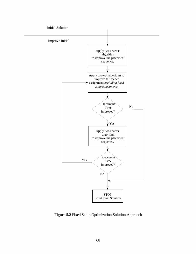
68
Improve Initial
Initial Solution
Apply two reversealgorithm
to improve the placementsequence.
Apply two opt algorithm toimprove the feeder
assignment excluding fixedsetup components.
PlacementTime
Improved?
Apply two reverse algorithm
to improve the placementsequence.
Improved?
Yes
No
Yes
No
STOPPrint Final Solution
PlacementTime
Figure 5.2 Fixed Setup Optimization Solution Approach

69
5.3 Calculation of Lower Bound
The lower bound was developed taking into account the functional characteristics of the Chip
Shooter machine. The following list describes the important functional characteristics of the
Chip Shooter machine that are considered when developing the lower bound equation.
1. The first NH/2 components in the placement sequence are already loaded in the turret head
when the component placement starts. In actual operations, the loading of the first NH/2
components is done while the next PCB is being loaded into the machine.
2. The placement time associated with the first component placement is the fixed pick and place
time (FPP) since the turret, feeder carriage, and PCB table are already in position for the first
placement and component pickup.
3. The turret rotation time associated with the ith component placement is dictated by the
component with the lowest STR loaded in the turret.
4. The minimum feasible placement time associated with the ith component placement except
for the first component placement, is the MRT/STR[i] . Note that in order to place a
component, the turret must rotate to the placement position. In the best case scenario, the
other components loaded in the turret have a higher STR, therefore the component being
placed is rotated to the placement position at its specified turret rotation rate.
From functional characteristic 1, 2, 3, and 4 it can be seen that it is beneficial to mount the
components with the slowest turret rotation rate (lowest STR) first. Remember low STR means
long turret rotation movement times. From 1 it is advantageous to place the components with the
lowest STR first because no time is incurred when loading the first NH/2 components in the
turret. This means that there are NH/2 free turret rotation movements. Therefore by assigning
the components with the slowest turret rotation rate (lowest STR) to be the first NH/2
placements, the turret rotation movement time savings are maximized. In addition, from 2 it can
be observed that the first component placement is free of movement time (only the FPP is

70
incurred). Thus, more time can be saved by placing the component with the lowest STR first.
From 3 and 4 it can be observed that by placing the components with the lowest STRs first, none
of the components with a higher STR would ever have to be rotated at a lower STR since all the
components with a lower STR would have been placed by then. This gives the potential for each
component to be mounted at their specification turret rotation rate (STR). Based on these
characteristics it can be seen that the least feasible total placement time (lower bound) that can be
achieved assumes that the PCB table and the feeder carriage do not cause any delays and by
placing the components in ascending order of STR. The following example shows a set of
components placed in ascending order of STR versus descending order of STR. For this
example, the PCB table and feeder carriage movement times are ignored. Table 5.1 provides
machine data and Table 5.2 provides the component data.
Table 5.1 Lower Bound Calculation Machine Data
Number of turret heads 10Fixed Pick and Place time (FPP) sec. .03Minimum Turret Rotation Time (MRT) sec. .20
Table 5.2 Lower Bound Calculation Component Data
Component Number STR1 12 13 14 15 16 0.87 0.88 0.89 0.810 0.811 0.812 0.813 0.814 0.415 0.416 0.417 0.418 0.419 0.420 0.4

71
The machine has 10 turret heads. Therefore, the turret movement time associated with the ith
component placement is such that:
=+≤≤
][4
tr[i] STRMRT
maxtj
iji(15)
Table 5.3 shows the placement time associated with each component placement when placed in
ascending order of STR. Table 5.4 shows the placement time associated with each component
placement when placed in descending order of STR. The placement time of the first component
is the just the fixed pick and place time (FPP) as explained before, and the placement time of the
rest of the components is the sum of the FPP associated with each component placement and the
resulting turret rotation time calculated using Equation (15).
Table 5.3 Placement Time Based on Ascending STR Placement Sequence
ComponentNumber
STR ttr[i] FPP PT[i]
20 0.4 0 0.03 0.0319 0.4 0.5 0.03 0.5318 0.4 0.5 0.03 0.5317 0.4 0.5 0.03 0.5316 0.4 0.5 0.03 0.5315 0.4 0.5 0.03 0.5314 0.4 0.5 0.03 0.5313 0.8 0.25 0.03 0.2812 0.8 0.25 0.03 0.2811 0.8 0.25 0.03 0.2810 0.8 0.25 0.03 0.289 0.8 0.25 0.03 0.288 0.8 0.25 0.03 0.287 0.8 0.25 0.03 0.286 0.8 0.25 0.03 0.285 1 0.2 0.03 0.234 1 0.2 0.03 0.233 1 0.2 0.03 0.232 1 0.2 0.03 0.231 1 0.2 0.03 0.23
PT => 6.6

72
Using the suggested method to calculate the lower bound, the placement time of 6.6 seconds is
obtained if components are placed in ascending order of STR. On the other hand, if the
components are placed in descending order of STR, a placement time of 8.1 seconds is obtained
as shown in Table 5.4
Table 5.4 Placement Time Based on Descending STR Placement Sequence
ComponentNumber
STR ttr[i] FPP PT[i]
1 1 0 0.03 0.032 1 0.25 0.03 0.283 1 0.25 0.03 0.284 1 0.25 0.03 0.285 1 0.25 0.03 0.286 0.8 0.25 0.03 0.287 0.8 0.25 0.03 0.288 0.8 0.25 0.03 0.289 0.8 0.25 0.03 0.2810 0.8 0.5 0.03 0.5311 0.8 0.5 0.03 0.5312 0.8 0.5 0.03 0.5313 0.8 0.5 0.03 0.5314 0.4 0.5 0.03 0.5315 0.4 0.5 0.03 0.5316 0.4 0.5 0.03 0.5317 0.4 0.5 0.03 0.5318 0.4 0.5 0.03 0.5319 0.4 0.5 0.03 0.5320 0.4 0.5 0.03 0.53
PT => 8.1
As shown by the previous example, a lower bound can be computed by creating a placement
sequence in which the components are placed in ascending order of STR. The lower bound on
the placement time can then be obtained by adding the turret rotation times and the fixed pick
and place time associated with each component placement. In the case of the first component
placement, the turret rotation time is assumed to be zero. Since the components are placed in
ascending order of STR, the turret rotation time associated with the ith component placement is

73
such that:
][][
iitr STR
MRTt = . (16)
Incorporating Equation (16) into the calculation of the lower bound (LB) yields a lower bound
expression such that:
∑ ∑= =
+=NC
i
NC
ii
FPPSTR
MRTLB
2 1][. (17)
This lower bound expression is used for evaluating the results obtained using the proposed
solution approaches.
The remaining chapters of this thesis focus on testing the general solution approach and fixed
setup solution approach using real PCB data provided by the industrial partner, actual CP4-3
machine parameters, and the placement time estimator function developed for the CP4-3
machine. Chapter VI presents an industrial case study in which the general solution approach
and the fixed setup solution approach are tested using real PCB data. The results obtained are
then compared to those obtained with the commercial software used by the industrial partner.
The final results of the research and conclusions are presented and summarized in Chapter VII.

74
CHAPTER VI
CASE STUDY
This chapter presents an industrial case study to test the performance of the solution approaches
presented in Chapter V. The case study consists of determining the placement sequence and
feeder assignment for a set of PCBs for different setup strategies. The case study was conducted
for a Fuji CP4-3 machine in a production environment with medium production volume and
medium variety of PCB types at the industrial partner’s facility. The placement time estimator
function for the CP4-3 machine was developed in Chapter IV, and it is shown in Equation (13).
The proposed solution approaches were tested for three different machine setup strategies. The
general optimization solution approach was tested for the case in which the machine feeder
carriage has no component types assigned to it, and the component types of a PCB can be
assigned to any feeder slot. This machine setup strategy, also known as the free setup strategy, is
generally used for production environments with low product variety and high production
volume. Therefore, minimization of the processing time tends to have a higher priority than
minimization of the setup time.
The fixed setup optimization solution approach was tested for two different machine setup
strategies: the fixed setup strategy and the partial fixed setup strategy. With a fixed setup
strategy all the component types of the PCB have already been assigned to feeder slots on the
feeder carriage and they cannot be reassigned. This strategy is generally used when producing a
family of PCBs that are highly similar or in production environments with medium to high
product variety and medium to low production volumes. The objective of this setup strategy is
to eliminate or drastically reduce setup times by assigning the component type feeders for a
family or group of PCBs to the feeder carriage. At the industrial partner’s facility, the
assignment of feeders for a family of PCBs is usually performed by combining all the component
data from the PCBs in the family. Thus, a hypothetical PCB consisting of superimposed X and
Y coordinates of all the components used in all the PCBs included in the family is created. Then,
a feeder assignment for this hypothetical PCB is determined and used as the feeder assignment
for the entire PCB family.

75
The partial fixed setup strategy is when some of the component types used on a PCB have
already been assigned to the feeder carriage, and the feeder assignment of the remaining
component types is to be determined. This strategy is sometimes used when producing a family
of PCBs that are highly similar or in production environments with medium to high product
variety and medium to low production volumes. However, unlike the fixed setup strategy, the
assignment of component types to the feeder carriage for all the component types included in the
family of PCBs is not performed using a hypothetical PCB. Instead, the assignment of
component types for one specific PCB in the family is performed first, then the component types
used on another specific PCB in the family that have not been already assigned are assigned to
the feeder carriage. This process is repeated until all the component types in the family of PCBs
are assigned to the feeder carriage.
The solution approach presented in Chapter V was coded using Visual Basic [28] in conjunction
with Excel (version 97 SR-1) spreadsheets. The program was executed on a workstation with a
Pentium II 450 MHz processor and 128 MB of RAM. The computer program has an
optimization module, which optimizes the placement sequence and feeder assignment for a PCB.
In addition, the program includes an evaluation module that calculates the placement time
associated with any given placement sequence and feeder assignment included in a placement
program created by the commercial software use by the industrial partner. Figure 6.1 shows the
main control screen of the program.

76
Figure 6.1 Control Screen of Optimization and Evaluation Program
One of the features of the program is that it provides the user with real time status of the
optimization with a graph that indicates the percent improvement from the initial solution as the
solution is improved. In addition, the user may select the construction heuristic, select whether
or not to improve the initial solution, and specify a time limit on the execution of the
improvement heuristics.
In order to evaluate or optimize a placement sequence and feeder assignment for a PCB, some
component data has to be input to the evaluation and optimization modules respectively. The
necessary component data includes:
• The component names,
• The X and Y coordinates of each component on the PCB,
• The PCB table speed setting (STS) associated with each component type, and
• The turret rotation rate (STR) associated with each component type.

77
The following sections describe in detail the results from the case study for each of the machine
setup strategies previously described.
6.1 Free Setup Case Study Results
As described earlier, the free setup strategy is one in which all the component types of the PCB
have to be assigned to the feeder carriage and the component placement sequence determined.
The component data for four PCBs were gathered from the industrial partner’s facility. The
component data was evaluated to determine a lower bound on the placement time. In addition,
the feeder assignment and placement sequence generated by the commercial software were
obtained for comparison purposes. These were input to the evaluation module and the
component placement time calculated. The component data for each of the PCBs was input to
the optimization module to construct and optimize a component placement sequence and feeder
assignment. Note that since this is the free setup strategy, the solution approach used by the
optimization module is the general optimization solution approach described in Section 5.1.
Table 6.1 shows the component data for each PCB.
PCB 4 is not an actual PCB, but instead a combination of several PCBs with their X and Y
coordinates superimposed on top of each other. This hypothetical PCB was created to test the
performance of the general optimization solution approach on a very large scale problem.
Table 6.1 Free Setup Component Data
PCBName
Number ofComponents on PCB
Number of Component Types on PCB
1 129 192 211 643 272 404 1661 69
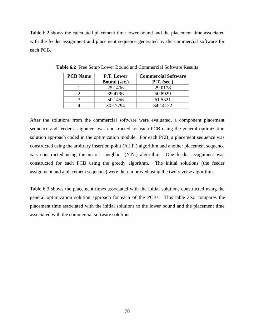
78
Table 6.2 shows the calculated placement time lower bound and the placement time associated
with the feeder assignment and placement sequence generated by the commercial software for
each PCB.
Table 6.2 Free Setup Lower Bound and Commercial Software Results
PCB Name P.T. LowerBound (sec.)
Commercial SoftwareP.T. (sec.)
1 25.1406 29.01782 39.4796 50.89293 50.1456 61.55214 302.7794 342.4122
After the solutions from the commercial software were evaluated, a component placement
sequence and feeder assignment was constructed for each PCB using the general optimization
solution approach coded in the optimization module. For each PCB, a placement sequence was
constructed using the arbitrary insertion point (A.I.P.) algorithm and another placement sequence
was constructed using the nearest neighbor (N.N.) algorithm. One feeder assignment was
constructed for each PCB using the greedy algorithm. The initial solutions (the feeder
assignment and a placement sequence) were then improved using the two reverse algorithm.
Table 6.3 shows the placement times associated with the initial solutions constructed using the
general optimization solution approach for each of the PCBs. This table also compares the
placement time associated with the initial solutions to the lower bound and the placement time
associated with the commercial software solutions.

79
Table 6.3 Free Setup Initial Solution Results
PCBName
ConstructionAlgorithm
InitialSolution
P.T. (sec.)
Percent Above Lower Bound P.T.
Percent Below P.T. of Commercial Software
1 A.I.P 28.8085 14.59% 0.72%1 N.N. 28.7933 14.53% 0.77%2 A.I.P 50.1403 27.00% 1.48%2 N.N. 47.3844 20.02% 6.89%3 A.I.P. 57.8401 15.34% 6.03%3 N.N. 58.3959 16.45% 5.13%4 A.I.P. 337.7970 11.57% 1.35%4 N.N. 339.6924 12.19% 0.79%
For all three PCBs, the constructed initial solutions have a lower placement time than the
commercial software solutions. For two of the four PCBs the A.I.P. algorithm yielded lower
placement times than the N.N. algorithm.
After the initial solution is constructed, the two reverse improvement algorithm is applied to each
of the initial solutions. Table 6.4 summarizes the improved solution results from the two reverse
algorithm. The table compares the placement time associated with the improved solutions to the
lower bound and the placement time associated with the commercial software solutions.
Table 6.4 Free Setup Improved Solution Results
PCBName
ConstructionAlgorithm
ImprovedSolution
P.T. (sec.)
Percent Above Lower Bound
P.T.
Percent Below P.T.of Commercial
Software1 A.I.P 27.6306 9.90% 4.78%1 N.N. 28.7359 11.91% 3.04%2 A.I.P 46.4836 17.74% 8.66%2 N.N. 46.2674 17.19% 9.09%3 A.I.P. 56.2610 12.20% 8.60%3 N.N. 56.3835 12.44% 8.40%
* 4 A.I.P. 336.7779 11.23% 1.65%* 4 N.N. 338.5716 11.82% 1.12%
* Indicates the improvement procedure was only run for 12 hours.

80
For three of the PCBs, the improved solutions that were initially constructed with the A.I.P.
algorithm yielded lower placement times than the improved solutions that were initially
constructed with the N.N. algorithm for all three PCBs.
The computation times associated with the construction of the initial solutions and the
improvement of the initial solutions for each of the PCBs are shown in Table 6.5.
Table 6.5 Free Setup Solution Computation Times
PCBName
ConstructionAlgorithm
Initial Solution Computation Time
(sec.)
Improved Solution Computation Time
(sec.)1 A.I.P 2 15861 N.N. 1 33222 A.I.P. 3 280532 N.N. 3 127833 A.I.P. 5 404623 N.N. 5 43959
* 4 A.I.P. 164 43200* 4 N.N. 152 43200
* Indicates the improvement procedure was only run for 12 hours.
The computation times associated with the construction of the initial solutions are similar for
both of the construction algorithms (A.I.P. and N.N.). The computation times associated with
the improvement of the initial solutions constructed with the A.I.P. algorithm and the N.N.
algorithm vary depending on the placement time associated with the initial solution. For each
PCB, the construction algorithm (A.I.P. or N.N.) which generated the initial solution with the
smallest placement time has the smallest computation time associated with the improved
solution. The reason for this is that the initial solutions with a large placement time have more
potential for improvement and are improved for a longer amount of time.

81
6.2 Fixed Setup Case Study Results
As mentioned earlier, the fixed setup strategy is one in which all the component types of the PCB
have already been assigned to the feeder carriage and only the component placement sequence
has to be determined. The total number of component types in the fixed setup includes all the
component types used on a family of PCBs. For this case study, five different PCBs were
included in the family. The component data and the PCB family feeder assignment for the five
PCBs were gathered from the industrial partner’s facility. The placement sequence generated by
the commercial software for each of the PCBs was also gathered for comparison purposes. Table
6.6 shows the component data for each PCB.
Table 6.6 Fixed Setup Component Data
PCBName
Number ofComponents
on PCB
Number ofComponent
Types onPCB
Total Number ofComponent
Types in Fixed Setup
5 48 29 1186 56 15 1187 73 21 1188 94 11 1189 211 64 118
The component data was input to the evaluation module and a lower bound placement time was
calculated for each PCB. The PCB family feeder assignment and placement sequence generated
by the commercial software for each of the PCBs were also input to the evaluation module to
calculate their corresponding placement time. Table 6.7 shows the calculated placement time
lower bound and the placement time associated with the commercial software solutions.
Table 6.7 Fixed Setup Lower Bound and Commercial Software Results
PCB Name P.T. Lower Bound(sec.)
Commercial Software P.T.(sec.)
5 9.0783 17.18126 10.9162 18.15167 15.0374 23.31438 17.9758 25.26399 39.4796 54.4889

82
After evaluating the commercial software solutions, the component data for each PCB and the
PCB family feeder assignment were input to the optimization module. Using the fixed setup
optimization solution approach coded in the optimization module a placement sequence was
constructed for each PCB and their corresponding placement time calculated. Two different
placement sequences were constructed for each PCB, one using the arbitrary insertion point
(A.I.P.) algorithm and another using the nearest neighbor (N.N.) algorithm. Table 6.8 shows the
placement times associated with the initial solutions constructed using the fixed setup
optimization solution approach for each of the PCBs. The table also compares the placement
time associated with the initial solutions to the lower bound and the placement time associated
with the commercial software solutions.
Table 6.8 Fixed Setup Initial Solution Results
PCBName
ConstructionAlgorithm
InitialSolution
P.T. (sec.)
Percent Above Lower Bound
P.T.
Percent Below P.T. of Commercial Software
5 A.I.P 17.5495 93.31% -2.14%5 N.N. 23.2381 155.97% -35.25%6 A.I.P. 17.1639 57.23% 5.44%6 N.N. 18.3305 67.92% -0.99%7 A.I.P 22.3522 48.64% 4.13%7 N.N. 24.6176 63.71% -5.59%8 A.I.P. 25.7474 43.23% -1.91%8 N.N. 25.3179 40.84% -0.21%9 A.I.P. 54.2016 37.29% 0.53%9 N.N. 58.7874 48.91% -7.89%
From Table 6.8, it can be observed that for four out of the five PCBs the A.I.P. algorithm
provided initial solutions with lower placement times than those constructed with the N.N. For
three of the PCBs, the A.I.P. algorithm generated initial solutions with lower placement time
than the commercial software solutions. For all five PCBs, the N.N. algorithm generated initial
solutions with longer placement times than the commercial software.
After constructing the initial placement sequences, these were improved using the two reverse
improvement algorithm. Table 6.9 shows the placement times associated with the improved

83
solutions, compares the placement time associated with the initial solutions to the lower bound
and the placement time associated with the commercial software solutions.
Table 6.9 Fixed Setup Improved Solution Results
PCBName
ConstructionAlgorithm
ImprovedSolution
P.T. (sec.)
Percent Above Lower Bound
P.T.
Percent Below P.T.of Commercial
Software5 A.I.P 16.3059 79.61% 5.09%5 N.N. 16.4265 80.94% 4.39%6 A.I.P. 16.4662 50.84% 9.29%6 N.N. 16.618 52.23% 8.45%7 A.I.P 21.3577 42.03% 8.39%7 N.N. 21.3543 42.01% 8.41%8 A.I.P. 24.7255 37.55% 2.13%8 N.N. 24.7665 37.78% 1.97%9 A.I.P. 50.0922 26.88% 8.07%9 N.N. 50.4734 27.85% 7.37%
From Table 6.9 it can be observed that after the two reverse algorithm was applied, the improved
solutions for the five PCBs have a lower placement time than the commercial software solutions
regardless of which algorithm was used to construct the initial solution. For each PCB, the
solutions obtained after the two reverse algorithm was applied to improve the initial solutions
constructed with the A.I.P. and N.N. algorithm differ slightly on placement time. However, in
four out of the five PCBs, the improved solutions that were initially constructed with the A.I.P.
algorithm yield slightly lower placement times than those that were initially constructed with the
N.N. algorithm. Table 6.10 shows the computation time associated with the construction of the
initial solutions and the improved solutions.

84
Table 6.10 Fixed Setup Solution Computation Times
PCBName
ConstructionAlgorithm
Initial Solution Computation Time
(sec.)
Improved Solution Computation Time
(sec.)5 A.I.P <1 565 N.N. <1 1266 A.I.P. <1 506 N.N. <1 607 A.I.P 1 2537 N.N. 1 3218 A.I.P. 1 4388 N.N. 1 6229 A.I.P. 4 196459 N.N. 4 25102
The computation times associated with the construction of the initial solutions are approximately
the same for both of the construction algorithms. However, the computational time associated
with improving the initial solutions constructed with the A.I.P. algorithm are appreciably lower
than the computational time associated with improving the initial solutions constructed with the
N.N. algorithm. In general, the initial solutions constructed with the A.I.P. algorithm are better
than those constructed with the N.N. algorithm and therefore require less improvement.
6.3 Partial Fixed Setup Case Study Results
As mentioned earlier, the partial fixed setup strategy is when part of the component types on a
PCB have already been assigned to the feeder carriage, and the assignment of the remaining
component types and placement sequence are to be determined. When constructing a feeder
assignment for the component types used on a PCB, the total number of component types already
assigned to the feeder carriage consists of the component types of the PCBs whose feeder
assignment has already been determined. The component types already assigned to the feeder
carriage may or may not include some of the component types used on the PCB whose feeder
assignment and placement sequence is being constructed.

85
The partial fixed setup strategy is used when producing a family of PCBs. The difference
between the partial fixed setup strategy and the fixed setup strategy is that in the fixed setup
strategy all the component types of all the PCBs in the family are assigned to the feeder carriage.
In the partial fixed setup strategy the assignment of component types for one specific PCB in the
family is performed first, then the component types on another specific PCB in the family that
have not been already assigned in the previous PCBs are assigned to the feeder carriage. This
step is repeated until all the component types used in the PCBs included in the family are
assigned to the feeder carriage.
The component data for a family of six PCBs was gathered from the industrial partner’s facility
and evaluated to determine a placement time lower bound for each PCB. The feeder assignment
and placement sequence generated by the commercial software were also gathered for
comparison purposes. Only five of the PCBs from the family of six PCBs were selected for this
case study. The PCB in the family, whose feeder assignment was constructed first, using the
commercial software was omitted. The reason for this is that when constructing the feeder
assignment for the first PCB in the family there are no component types with pre-assigned feeder
carriage locations. Thus, it does not fit the partial fixed setup strategy, but instead it falls under
the free setup strategy. Table 6.11 shows the component data for each PCB.
Table 6.11 Partial Fixed Setup Component Data
PCBName
Number ofComponents
on PCB
Number ofComponent
Types onPCB
Number ofPre – Assigned
ComponentTypes on PCB
Total Number ofPre - Assigned
ComponentTypes on Feeder
Carriage
Total Number ofComponent
Types on FeederCarriage After
Assignment10 286 55 21 40 7411 136 16 10 74 8012 134 18 16 80 8213 36 16 9 82 8914 60 4 2 89 91
The total number of component types assigned to the feeder carriage before the assignment of
the component types of PCB 10 is 40 component types. These are the component types used on
the PCB whose component types were assigned to the feeder carriage first. As mentioned before
this PCB is not included in this section since it falls under the free setup strategy. PCB 10 has a
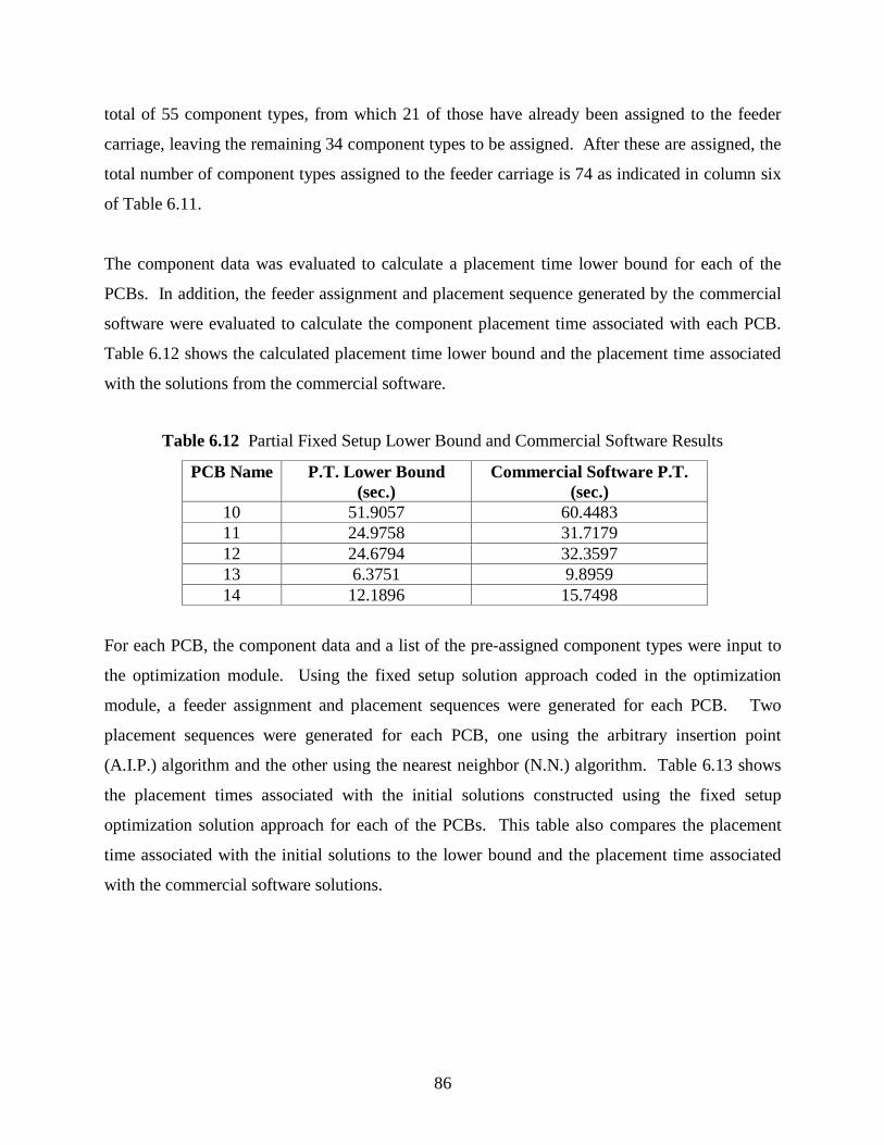
86
total of 55 component types, from which 21 of those have already been assigned to the feeder
carriage, leaving the remaining 34 component types to be assigned. After these are assigned, the
total number of component types assigned to the feeder carriage is 74 as indicated in column six
of Table 6.11.
The component data was evaluated to calculate a placement time lower bound for each of the
PCBs. In addition, the feeder assignment and placement sequence generated by the commercial
software were evaluated to calculate the component placement time associated with each PCB.
Table 6.12 shows the calculated placement time lower bound and the placement time associated
with the solutions from the commercial software.
Table 6.12 Partial Fixed Setup Lower Bound and Commercial Software Results
PCB Name P.T. Lower Bound(sec.)
Commercial Software P.T.(sec.)
10 51.9057 60.448311 24.9758 31.717912 24.6794 32.359713 6.3751 9.895914 12.1896 15.7498
For each PCB, the component data and a list of the pre-assigned component types were input to
the optimization module. Using the fixed setup solution approach coded in the optimization
module, a feeder assignment and placement sequences were generated for each PCB. Two
placement sequences were generated for each PCB, one using the arbitrary insertion point
(A.I.P.) algorithm and the other using the nearest neighbor (N.N.) algorithm. Table 6.13 shows
the placement times associated with the initial solutions constructed using the fixed setup
optimization solution approach for each of the PCBs. This table also compares the placement
time associated with the initial solutions to the lower bound and the placement time associated
with the commercial software solutions.

87
Table 6.13 Partial Fixed Setup Initial Solution Results
PCBName
ConstructionAlgorithm
InitialSolution
P.T. (sec.)
Percent Above Lower Bound
P.T.
Percent Below P.T. of Commercial Software
10 A.I.P 59.488 14.61% 1.59%10 N.N. 62.4484 20.31% -3.31%11 A.I.P. 31.4589 25.96% 0.82%11 N.N. 33.1821 32.86% -4.62%12 A.I.P. 33.1097 34.16% -2.32%12 N.N. 33.9545 37.58% -4.93%13 A.I.P. 10.2143 60.22% -3.22%13 N.N. 9.8755 54.91% 0.21%14 A.I.P. 15.8619 30.13% -0.71%14 N.N. 16.3047 33.76% -3.52%
From Table 6.13, it can be observed that for four out of the five PCBs the A.I.P. algorithm
provided initial solutions with lower placement times than those constructed with the N.N.
algorithm. For two of the PCBs the A.I.P. algorithm generated initial solutions with lower
placement time than the commercial software solutions, and for one PCB the N.N. algorithm
generated an initial solution with a lower placement time than the commercial software.
After constructing the initial solutions, the placement sequence and feeder assignment of each
PCB were improved using the two reverse algorithm and the modified two opt algorithm,
respectively. Table 6.14 shows the placement times associated with the improved solutions
improved using the two reverse and modified two opt algorithms. This table also compares the
placement time associated with the improved solutions to the lower bound and the placement
time associated with the commercial software solutions.

88
Table 6.14 Partial Fixed Setup Improved Solution Results
PCBName
ConstructionAlgorithm
ImprovedSolution
P.T. (sec.)
Percent Above Lower Bound
P.T.
Percent Below P.T. of Commercial Software
10 A.I.P 58.3150 12.35% 3.53%10 N.N. 58.8019 13.29% 2.72%11 A.I.P. 30.5944 22.50% 3.54%11 N.N. 30.4553 21.94% 3.98%12 A.I.P 30.9952 25.59% 4.22%12 N.N. 31.409 27.27% 2.94%13 A.I.P. 9.6047 50.66% 2.94%13 N.N. 9.5485 49.78% 3.51%14 A.I.P. 15.2338 24.97% 3.28%14 N.N. 15.2422 25.04% 3.22%
From Table 6.14 it can be observed that after applying the improvement algorithms, the
improved solutions for the five PCBs have a lower placement time than the commercial software
solutions regardless of which algorithm was used to construct the initial solution. For three out
of the five PCBs, the improved solutions that were initially constructed with the A.I.P. algorithm
yield slightly lower placement times than those that were initially constructed with the N.N.
algorithm.
Table 6.15 Partial Fixed Setup Solution Computation Times
PCBName
ConstructionAlgorithm
Initial Solution Computation Time
(sec.)
Improved Solution Computation Time
(sec.)10 A.I.P 16 4443710 N.N. 16 9237211 A.I.P. 2 197511 N.N. 2 553912 A.I.P 2 471412 N.N. 2 295313 A.I.P. <1 4213 N.N. <1 2014 A.I.P. <1 5114 N.N. 1 183
Table 6.15 shows the computation times associated with obtaining both the initial solutions and
the improved solutions. The initial solution computation times are minimal for each of the board

89
types and tend to vary with the board characteristics. The computation times for the improved
solutions are longer and also tend to vary with the board characteristics. PCB 10, with the
longest computation times, has a total of 286 components (55 types of components) that are
placed by the Chip Shooter machine. In addition, 34 of the component types need to be assigned
to feeder locations. On the other hand, PCB 13, with the shortest computation time, has a total of
36 components (16 types of components) that are placed by the Chip Shooter machine. Only 7
of the component types need to be assigned to feeder locations.
The computation times associated with the construction of the initial solutions are similar for
both of the construction algorithms. For three out of the five PCBs, the computational time
associated with the improved solutions initially constructed with the A.I.P. algorithm are
significantly lower than the computational times associated with the improved solutions initially
constructed with the N.N. algorithm.
6.4 Summary of Case Study Results
In general, regardless of the setup strategy, the A.I.P. algorithm often provides initial solutions
with lower placement times and similar computational times to those of the N.N. algorithm.
After the initial solutions are improved, those that were initially constructed with the A.I.P.
algorithm tend to have a lower placement time and shorter computational time than those that
were initially constructed with the N.N. algorithm.
For the free setup strategy, the feeder assignment and placement sequence of four PCBs were
constructed using the A.I.P. algorithm and N.N. algorithm. For all four PCBs the initial
solutions constructed with the A.I.P. algorithm and the ones constructed with the N.N. algorithm
had a lower placement time than the solutions from the commercial software. For the fixed and
partially fixed setup strategies in three out of the five PCBs used in the studies, at least one of the
initial solutions constructed with either the A.I.P. algorithm or the N.N. algorithm had lower
placement times than the commercial software. For all the setup strategies and PCBs used in the

90
case study, the placement times associated with the improved solutions always had a lower
placement time than the solutions from the commercial software.
From the results presented in this chapter, it can be observed that the placement times associated
solutions obtained in the free setup strategy case study are significantly closer to the lower bound
than the placement times associated solutions obtained for the fixed setup strategy and partially
fixed setup case studies. As mentioned earlier, for the fixed and partially fixed setup strategies,
the assignment of component types to the feeder carriage is performed for a family of PCBs, so
the feeder carriage contains component types for multiple PCBs. Therefore, for one specific
PCB within the family, the feeder assignment may be such that the component types used on the
PCB are not located close together in the feeder carriage, instead component types used in other
PCBs of the PCB family may separate them. This cause long feeder movements, which increase
the placement time. However, an advantage of the fixed and partially fixed setup strategies is
that for production scenarios with high product mix, and low volume, these setup strategies
eliminate or drastically reduce setup times. Since the feeder carriage is setup for a family of
PCBs, no setups are required in between production runs of PCBs from the same family. On the
other hand, the free setup strategy provides smaller component placement times, but requires the
setup of the feeder carriage each time a different PCB type is produced. Therefore, increasing
the setup time.
The component data, commercial software solutions, and the solutions obtained using the
solution approaches presented in this research for PCBs 1, 5, and 13 included in the free, fixed,
and partially fixed setup case studies, respectively, are attached in Appendix C.

91
CHAPTER VII
CONCLUSIONS AND AREAS OF FURTHER RESEARCH
7.1 Conclusions
This research has addressed two of the decision problems associated with process optimization in
printed circuit board assembly systems for a specific assembly machine. Specifically, a solution
approach was developed for determining the component placement sequence and feeder
assignment for a turret style Chip Shooter type machine. These decisions are performed
following the allocation of component types to the different machines in the SMT line. To
address these decisions, the solution approach develop in this research:
• Sequences the components to be mounted by the machine on the PCB, and
• Assigns component types to the slots in the machine feeder carriage.
The turret style Chip Shooter machine consists of three primary mechanisms: the turret, the PCB
table, and the feeder carriage. The turret contains an even number of placement heads and
transports the components from the feeder carriage to the PCB table. The PCB table secures the
PCB and locates the PCB under the placement station in the location where the component
loaded has to be mounted. The feeder carriage mechanism stores the component feeders that
contain a component tape reel. The function of the feeder carriage is to position the feeder of the
component to be retrieved under the grip station. Since all the mechanisms move independently
and simultaneously, the time to place a component is determined by the mechanism that takes the
longest movement time in the cycle. Therefore, the sequence in which the components are placed
on the PCB and the arrangement of the feeders in the feeder carriage affects the assembly cycle
time.
This research has presented a new solution approach to determine the placement sequence and
feeder assignment of components for the Chip Shooter type machine with the objective of
minimizing cycle time and generating additional production capacity. In order to remain

92
competitive in the PCB manufacturing industry, resources must be utilized efficiently.
Therefore, any gain in production capacity is highly valuable.
A component placement time estimator function for the Chip Shooter type machine was
developed in Section 4.2. The placement time estimator function accounts for the functional
characteristics of the Chip Shooter machine. A placement time estimator function for the Fuji
CP4-3 Chip Shooter machine was developed in Section 4.3.2. This was developed by
incorporating the component placement time estimator function for the Chip Shooter type
machine with the experimental velocity functions developed in Section 4.3.1 for each of the
mechanisms of the CP4-3 machine.
The component placement sequence and feeder assignment problems are both considered NP
complete. Thus, a heuristic solution approach was developed in Chapter V. Two solution
approaches have been developed:
• The general optimization solution approach presented in Section 5.1, and
• The fixed setup optimization solution approach presented in Section 5.2.
The general optimization solution approach determines the placement sequence and feeder
assignment for a PCB when all the slots in the feeder carriage are available for the feeder
assignment. The fixed setup optimization solution approach determines the placement sequence
and feeder assignment for the fixed setup scenario, in which some or all of the component
feeders are fixed to pre specified feeder slots and can not be re-assigned. Both of these solution
approaches were coded using Visual Basic in conjunction with Excel spreadsheets. A case study
was conducted to validate the proposed solution approaches for the Fuji CP4-3 machine.
The general optimization solution approach was tested using actual component data from three
PCBs produced by an industrial partner. The solutions obtained were compared to those
obtained using the commercial software used by the industrial partner. For all four PCBs the
component placement times obtained using the general optimization solution approach were
lower than those obtained using the commercial software.

93
The fixed setup optimization solution approach was tested for two different machine setup
strategies using actual component data from two sets of five PCBs produced by the industrial
partner. For both of these setup strategies the solutions obtained with the fixed setup
optimization solution approach yielded lower component placement times than those obtained
using the commercial software.
This research has been useful in making the following contributions:
• The relationship between the different Chip Shooter machine mechanisms was modeled;
• A general component placement time estimator function for the Chip Shooter type
machine was developed to account for the machine functional characteristics and the
component characteristics;
• Velocity functions for the Fuji CP4-3 machine mechanisms were generated
experimentally;
• A construction algorithm was developed based on a set of knowledge-based rules, which
takes advantage of the machine functional characteristics and component data to
construct an initial component placement sequence and feeder assignment for different
setup strategies;
• An improvement algorithm was developed using a modified two opt algorithm and the
two reverse algorithm to improve the initial placement sequence and feeder assignments
for different setup strategies; and
• The performance of the proposed solution approaches was tested and compared to state
of the art PCB assembly process optimization software.
• Increase SMT line production capacity by reducing the placement time at the Chip
Shooter type machines.
7.2 Areas For Further Research
Several areas for further research have been identified while conducting this research. As
mentioned earlier, the research presented has focused specifically on the turret style Chip
Shooter machine. One of the areas for further research would be to develop solution approaches

94
that incorporate theoretical research findings and account for the machine functional
characteristics for other types of assembly machines, such as Gantry type machine.
Another area of further research would be to incorporate the decisions of component allocation
with the decisions of the component placement sequencing and feeder assignment associated
with each assembly machine in the line. Currently when performing the component allocation to
the different assembly machines within an SMT line to balance the workload, the placement time
of the component types is assumed to be constant and only dependent on the characteristics of
the component type and the machine types. In reality, however, the placement time of a
component depends on the placement sequence and the feeder assignment. A solution approach
that iteratevly or simultaneously considers the component allocation and feeder assignment and
placement sequencing decisions could be developed to improve process planning decisions.
Likewise, a challenging area for further research would be to address the problem of allocating
families of PCBs to different SMT lines with the objective of balancing the workload across
SMT lines, while simultaneously balancing the workload across the assembly machines within
each SMT line and optimizing the placement sequence and feeder assignment for each family of
PCBs.
Finally, another area for further research would be to create an algorithm that allocates
components to the different SMT machines in an SMT line or even in several SMT lines and
creates the component placement sequence and feeder assignment for each machine with the
objective of minimizing cycle time and quality problems. For example, some machines may be
better than others for placing specific components in terms of accuracy and precision. Also,
when creating the placement sequence of components it may be better to place specific
components at the end of the placement sequence due to possible quality problems such as
misalignment of components due to repeated PCB table movements. Currently there exist some
standards that specify which machines can place specific components and the rate at which they
should be placed, however, within these standards there is a large amount of options for each
component.

95
This research has showed that the total component placement time associated with the mounting
of components on a PCB depends on the component placement sequence and feeder assignment.
Therefore if the feeder assignment and component placement sequence decisions could be
incorporated with the higher level decisions (such as line balancing or workload balancing across
several SMT lines) more accurate process plans could be developed.
96
REFERENCES
[1] Agrawal, M.K. and Brinkley, P.A., “Optimizing Chip Placement Sequence in SMT
Operations,” Surface Mount Techniques,
http://www.smartlink.net/~bmcd/semi/mag/gluemach.htm.
[2] Ahmadi, J., Ahmadi, R., Matsuo, H., Tirupati, D., “Component Fixture
Positioning/Sequencing for Printed Circuit Board Assembly with Concurrent Operations,”
Operations Research, Vol. 43, No. 3, pp. 444-457, 1995.
[3] Ammons, J.C., Carlyle, M., G.W. Depuy, Ellis, K.P., McGinnis, L.F., Tovey, C.A., Xu, H.,
“Computer-Aided Process Planning in Printed Circuit Card Assembly,” IEEE Transactions
on Components, Hybrids, and Manufacturing Technology, Vol. 16, No. 4, pp. 370-376, 1993.
[4] Ammons, J.C., Carlyle, M., G.W. Depuy, Ellis, K.P., McGinnis, L.F., Tovey, C.A., Xu, H.,
“Component Allocation to Balance Workload in Printed Circuit Board Assembly Systems,”
IIE Transactions, Vol. 29, pp. 265-275 1997,
[5] Balakrishnan, V. K., “Network Optimization,” Chapman & Hall, 1995.
[6] Ball, M. O.and Magazine, M. J., “Sequencing of Insertions in Printed Circuit Board
Assembly,” Operations Research, Vol. 36, No. 2, pp. 192-201, 1988.
[7] Bellman, Cooke and Lockett, “Algorithms, Graphs, and Computers,” Academic Press, Inc.,
1970.
[8] Chan, D. and Mercier, D., “IC Insertion: an Application of the Travelling Salesmen Problem,”
International Journal of Production research, Vol. 27, No. 10, pp. 1837-1841, 1989.
[9] Chiang, W. and Chiang, C., “Intelligent Local Search Strategies for Solving the Facility
Layout problems with the Quadratic Assignment problem Formulation,” European Journal of
Operational Research, Vol. 106, No. 2-3, pp. 457-488, 1998.
[10] Crama, Y., Flippo, O.E., Van de Klundert, J., Spieksma, F., “The Assembly of Printed Circuit
Boards: A Case with Multiple Machines and Multiple Board Types,” European Journal of
Operational Research, Vol. 98, pp. 457-472, 1997.
[11] De Souza, R. and Lijun, W., “Intelligent Optimization of Component Onsertion in Multi-Head
Concurrent Operation PCBA Machines,” Journal of Intelligent Manufacturing, Vol. 6, pp.
235-243, 1995.

97
[12] Drezner, Z. and Nof, S., “On Optimizing Bin Picking and Insertion Plans for Assembly
Robots,” IIE Transactions, Vol. 16, No. 3, pp. 262-270, 1984.
[13] E.L. Lawler, J.K. Lenstra, A.H. Rinooy Kan, D.B. Shmoys, “The Travelling Salesmen
Problem,” John Wiley and Sons, 1983.
[14] Electronic Trend Publications, Abstract of The Worldwide PCB Assembly Market,
http://www.electronictrendpubs.com/pcbassy.htm
[15] Ellis, K.P., McGinnis, L.F., Ammons, J.C., “Setup Management Issues in Printed Circuit Card
Assembly Systems,” 7th International Conference on Flexible Automation and Intelligent
Manufacturing, June 25-27, 1997.
[16] Frieze, A., M., Galbiati, G. and Maffioli, F., “On the Worst-case Performance of Some
Algorithms for the Asymmetric Travelling Salesman Problem,” Networks, Vol. 12, pp. 23-39,
1982.
[17] Fuji, Fuji Product Catalog
[18] Golden, B. and Skiscim, C., “Using Simulated Annealing to Solve Routing and Location
Problems,” Naval Research Logistics Quarterly, Vil. 33, pp. 261-279, 1986.
[19] Gronalt, M., Grunow, M., Gunther, H.O., Zeller, R., “A Heuristic for Component Switching
on SMT Placement Machines,” International Journal of Production Economics, Vol. 53, pp.
181-190, 1997.
[20] Huang, Y.W., Srihari, K., Adriance, J., Westby, G. “A Solution Methodology for the Multiple
Batch Surface Mount PCB Placement Sequence problem,” Journal of Electronic Packaging,
Vol. 116, pp. 282-289, 1994.
[21] Kirkpatrick, S., Gelatt, C.D., Vecchi, Jr., M.P., “Optimization by Simulated Annealing,”
Science, Vol. 220, No. 4598, pp. 671-680, 1983.
[22] Kumar, R. and Li, H., “Assembly Time Optimization for PCB Assembly,” Proceedings of the
American Control Conference, pp. 306, 1994.
[23] Leipala, T. and Nevalainen, O., “Optimization of the Movements of Component Placement
Machine,” European Journal of Operational Research, Vol. 38, pp. 167-177, 1989.
[24] Leu, M.C., Wong, H., Ji, Z. “Planning of Component Placement/Insertion Sequence and
Feeder Setup in PCB Assembly using Genetic Algorithm,” Transactions of the ASME, Vol.
115, pp. 424-432, 1993.
[25] Mandl, C., “Applied Network Optimization,” Academic Press, 1979.
98
[26] McGinnis, L.F., Ammons, J.C., Carlyle, M., Cranmer, L., Depuy, G.W., Ellis, K.P., Tovey,
C.A., Xu, H., “Automated Process Planning for Printed Circuit Card Assembly,” IIE
Transactions, Vol. 24, No. 4, pp. 18-30, 1992.
[27] Meller, R.D. and Bozer, Y.A., “A New Simulated Annealing Algorithm for the Facility
Layout Problem,” International Journal of Production Research, Vol. 34, No. 6, pp. 1675-
1692, 1996.
[28] Microsoft Corporation, Visual Basic User’s Guide, 1994.
[29] Moyer, L. K. and Gupta, S, M., “An Efficient Assembly Sequencing Heuristic for Printed
Circuit Boards Configurations,” Journal of Electronics Manufacturing, Vol. 7, No. 2, pp.
143-160, 1997.
[30] Moyer, L. K. and Gupta, S, M., “Simultaneous Component Sequencing and Feeder
Assignment for High Speed Chip Shooter Machines,” Journal of Electronics Manufacturing,
Vol. 6, No. 4, pp. 271-305, 1996.
[31] Moyer, L. K. and Gupta, S, M., “SMT Feeder Slot Assignment for Predetermined Component
Placement Paths,” Journal of Electronics Manufacturing, Vol. 6, No. 3, pp. 173-192, 1996.
[32] Noble, B. Provided Statistical Advice for the Analysis of the CP4-3 machine Experiments,
Virginia Tech Statistical Consulting Center, 1999.
[33] Otten, R. H. and Van Ginneken, L. P., “The Annealing Algorithm,” Kluwer Academic
Publishers, 1989.
[34] Press, W. H., Vetterling, W. T., Teukolsky, S. A., Flannery, B. P., “Numerical Recipes in
Fortran 77, 2nd ed.,” Cambridge University Press, 1996.
[35] Reeves, C. R., “An Improved Heuristic for the Quadratic Assignment Problem,” Journal of
Operational Research Society, Vol. 36, No. 2, pp. 163-167, 1985.
[36] Safai, F. “Cycle Time Improvement for Fuji IP2 Pick-and-Place Machines,” Hewlett-Packard
Journal, pp. 80, Aug., 1996.
[37] Smith, C. Provided Technical Advice for Developing the Improvement Heuristics, 1999.
[38] Smith, D. K., “Network Optimization Practice,” John Wiley & Sons, Inc., 1982.
[39] Sohn, J. and Park, S., “Efficient Operation of a Surface Mounting Machine with a Multihead
Turret,” International Journal of Production Research, Vol. 34, No. 4, pp. 1131-1143, 1996.
[40] The News and Observer Publishing Company Raleigh, Electronics Industry growth,
http://www.news-observer.com/daily/1997/10/31/biz01.html

99
[41] Van Breedam, A., “Improvement Heuristics for the Vehicle Routing Problem based on
Simulated Annealing,” European Journal of Operational Research, Vol. 86, pp. 480-490,
1995.
[42] Vidal, R. V., “Applied Simulated Annealing,” Springer-Verlag, 1993.

100
APPENDIX A
GENERAL OPTIMIZATION SOLUTION APPROACH EXAMPLE
Initial Solution Construction Example
In order to explain the initial solution construction procedure a detailed example is presented.
The data necessary to present the example includes machine data and PCB component data. The
machine data includes:
• the PCB table velocity functions for each table speed setting,
• the feeder carriage velocity function,
• the minimum turret rotation time (MTR),
• the fixed pick and place time (FPP),
• the number of placement heads in the turret, and
• the feeder slots capacity of the machine.
The PCB component data includes:
• the number of components to be mounted,
• the component number designated to each component,
• the component type associated with each component,
• the STR associated with each component type,
• the STS associated with each component type,
• the feeder size associated with each component type, and
• the X and Y coordinates associated with each component on the PCB.
Table A.1 and Table A.2 show all the necessary machine and PCB component data respectively.

101
Table A.1 General Optimization Machine Data
Number of Heads (NH) 6Number of Feeder Slots 20Minimum Turret Rotation Time (MRT) 0.15Fixed Pick and Place Time (FPP) 0.03High PCB Table Speed Setting (0) Velocity FunctionX-direction (mm/sec.)
Vx[0] = 10 + 6 (|X[i] -X[i-1] |)
High PCB Table Speed Setting (0) Velocity FunctionY-direction (mm/sec.)
Vy[0] = 10 + 6 (|Y[i] -Y[i-1] |)
Low PCB Table Speed Setting (1) Velocity FunctionX-direction (mm/sec.)
Vx[1] = 7 + 3 (|X[i] -X[i-1] |)
Low PCB Table Speed Setting (1) Velocity FunctionY-direction (mm/sec.)
Vy[1] = 7 + 3 (|Y[i] -Y[i-1] |)
Feeder Carriage Velocity Function (slots/sec.) Vfc = 5+5 (Ln(|FS[j] -FS[j-1] |))
Table A.2 General Optimization PCB Component Data
ComponentNumber
ComponentType
STR STS Feeder Size(mm)
X-Location(mm)
Y-Location(mm)
1 1 0.8 0 8 257.9 82.382 7 0.8 0 8 245.2 105.243 1 0.8 0 8 226.91 171.284 2 0.8 0 8 187.29 82.895 2 0.8 0 8 189.32 71.726 3 1 0 8 257.9 84.427 8 1 0 12 239.61 125.568 8 1 0 12 213.45 171.039 3 1 0 8 188.81 95.5910 4 1 0 8 257.9 86.4511 4 1 0 8 246.73 165.9512 4 1 0 8 202.53 170.7813 8 1 0 12 189.83 84.9214 5 0.4 1 12 243.17 90.7715 5 0.4 1 12 249.52 172.0516 5 0.4 1 12 195.16 141.8217 5 0.4 1 12 184.75 79.0818 6 0.4 1 16 240.63 81.3719 6 0.4 1 16 239.11 171.2820 6 0.4 1 16 192.37 95.5921 9 1 1 12 185.3 82.3222 9 1 1 12 187.63 86.3723 9 1 1 12 189.1 87.21

102
Step 1: For the set of NC = 23 components, divide the set into G groups of components having
the same specification table speed setting (STS) and turret rotation rate (STR). In this case since
there are two different STSs (0 and 1), and within each STS group there are two different STRs
(0.8 and 1 for STS = 0 and 0.4 and 1 for STS = 1). Therefore, G is equal to four. The groups are
formed by the following component numbers:
• Group 1, STS = 0, STR = 0.8, component numbers {1, 2, 3, 4, 5}.
• Group 2, STS = 0, STR = 1, component numbers {6, 7, 8, 9, 10, 11, 12, 13}.
• Group 3, STS = 1, STR = 0.4, component numbers {14, 15, 16, 17, 18, 19, 20}.
• Group 4, STS = 1, STR = 1, component numbers {21, 22, 23}.
Step 2: For each group G, construct an initial component placement sequence that minimizes the
PCB table movement time (ttb) using the nearest neighbor algorithm (N.N.) starting with the
component with the largest X coordinate. The N.N. algorithm consists of starting with one
component number and then finding its nearest neighbor (another component) based on the
calculated PCB table movement time matrix and assigning that nearest neighbor (component
number) next in the placement sequence [13]. The PCB table movement time matrix represents
the PCB table movement time to move between two specific components. The PCB table
movement time matrix (Table A.3) is calculated for the components in Group 1 using the ttb
metric from Equation (2) and substituting Vx[S] and Vy[S] with their corresponding functions
shown in Table A.1. Note that the units associated with the body of Table A.3 are in seconds.
Table A.3 General Optimization Group 1 PCB Table Movement Time Matrix
From Component -To Component 1 2 3 4 5
1 0 0.155341 0.1636 0.162823 0.1627122 0.155341 0 0.162564 0.162004 0.161843 0.1636 0.162564 0 0.163582 0.1639234 0.162823 0.162004 0.163582 0 0.1450275 0.162712 0.16184 0.163923 0.145027 0
After determining the PCB table movement time between all the components in the group, the
component number with the lowest X coordinate is chosen as the starting point for the N.N.
algorithm. For Group 1, component number 4 is selected as the starting point since it has the

103
lowest X coordinate (187.29 mm). The nearest neighbor algorithm is then applied and
component number 5 is selected as the next component in the sequence. This procedure is
repeated until all components in the group have been assigned to the placement sequence,
resulting in the following sequence {4, 5, 2, 1, 3}. The procedure is repeated for each group.
Table A.4 shows the resulting placement sequence for each group.
Table A.4 General Optimization Group Placement Sequences
Group 1 Component Number: 4, 5, 2, 1, 3Component Type : 2, 2, 7, 1, 1
Group 2 Component Number: 9, 13, 7, 10, 6, 11, 8, 12Component Type : 3, 8 , 8, 4 , 3, 4, 8, 4
Group 3 Component Number: 17, 20, 16, 19, 15, 14 , 18Component Type : 5 , 6 , 5, 6, 5, 5, 6
Group 3 Component Number: 21, 22, 23Component Type : 9 , 9, 9
Step 3: For each group G, construct a component type flow matrix using the placement
sequences generated in Step 3. If component type i is placed after component type j then the
flow between component types i and j and between component types j and i is increased by one.
Note that the flow between component types i and j is denoted by Fij . If i and j are the same
component type then Fij is equal to zero.
The component type flow matrix for group 1 is formed by the flows between component types 1,
2 and 7. The component type flow matrix for group 1 is calculated using the placement sequence
for group 1 in terms of component types {2, 2, 7, 1, 1} as shown in Table A.4. It can be
observed that there is one movement from component type 2 to component type 7 and one
movement from component type 7 to component type 1. The flows between same component
types are not counted. Therefore, the movement form component type 2 (component number 4)
to component type 2 (component number 5) and from component type 1 (component number 1)
to component type 1 (component number 3) are not counted and their flows are set equal to zero
(F11 = 0, F22 = 0). The remaining component type flows for group 1 are as follows: F12 = F21 = 0,
F17 = F71 = 1, F27 = F72 = 1. Tables A.5 to A.8 show the component type flow matrix for each
group. The headers of the columns and rows in the tables are the component types.

104
Table A.5 General Optimization Group 1 Component Type Flow Matrix
From-ToComponent Type 1 2 7
1 0 0 12 0 0 17 1 1 0
Table A.6 General Optimization Group 2 Component Type Flow Matrix
From-ToComponent Type
3 4 8
3 0 2 14 2 0 38 1 3 0
Table A.7 General Optimization Group 3 Component Type Flow Matrix
From-ToComponent Type
5 6
5 0 56 5 0
Table A.8 General Optimization Group 3 Component Type Flow Matrix
From-ToComponent Type
9
9 0
Step 4: For each group G, use a greedy algorithm to construct an initial feeder sequence that
minimizes the feeder carriage movement time (tfc). After constructing the feeder sequence
assign the components to the feeder carriage. Perform the assignment from the left of the feeder
carriage to the right starting with the group with the smallest STS (highest PCB table speed
setting) and smallest STR (slowest turret rotation rate) taking into account the feeder space
required by each component type.
The greedy algorithm starts the feeder sequence by selecting the two component types in the
group with the highest flow between them and creating an initial feeder sequence of two
component type numbers. The component type flow matrix is read from left to right and top to
bottom. Thus, if there is a tie between pairs of component types having the maximum flow, the

105
pair of components read first is selected to form the initial feeder sequence. The next component
type added to the feeder sequence is the one with the highest flow with one of the component
types at the extremes of the feeder sequence. Therefore, the component type to be added is
added either at the beginning or the end of the feeder sequence depending on which one has the
highest flow. If a tie occurs then the component type being added is added at the beginning of
the feeder sequence. Using the component type flow matrices shown in Tables A.5, A.6, A.7,
and A.8 the feeder sequence for each group can be constructed.
For group 1 using the component type flow matrix (Table A.5), the pair of component types 1
and 7 and 2 and 7 have the highest flows between them. Using the rule to break ties, component
types 1 and 7 are selected. Thus a partial feeder sequence for group 1 is form by component
types {1, 7}. This partial feeder sequence is then used with the remaining unassigned component
types to identify the one with the highest flow. In this case only component type 2 remains
unassigned and it has a flow of 1 with component type 7 and a flow of 0 with component type 1.
Therefore, it is assigned next to component type 7. The final feeder sequence for group 1 is {1,
7, 2}.
The same steps are repeated with the second, third, and fourth group. The partial feeder
sequences and final feeder sequences for all the groups are listed in Table A.9.
Table A.9 General Optimization Group Feeder Sequence
GroupNumber
Partial Feeder SequenceComponent Types
Final Feeder SequenceComponent Types
Group 1 {1, 7} {1, 7, 2}Group 2 {4, 8} {3, 4, 8}Group 3 {5, 6} {5,6}Group 4 {9} {9}
After constructing the feeder sequences for each group, the component types are assigned to
feeder slots from left to right in the feeder carriage beginning with the group with the lowest STS
and lowest STR. As shown in Table A.2, however, not all component types have the same
feeder size. For this example the feeder rules of the CP4-3 Fuji machine will be used. These
rules indicate that the center of the component feeder coincides with the center of the feeder

106
slots. In addition, component types with feeder size of 8 mm occupy only one feeder slot, and
component types larger than 8 mm occupy one feeder slot and half of the feeder slots adjacent to
it.
Using these rules, each of the component types in group 1 requires one feeder slot. Component
type 1 is assigned to feeder slot 1, component type 7 is assigned to feeder slot 2, and component
type 2 is assigned to feeder slot 3. The component types for group 2 are assigned next starting
from feeder slot 4, since the first three slots have already been assigned to the component types
of group 1. Component type 3 is assigned to feeder slot 4, component type 4 is assigned to
feeder slot 5, and component type number 8 is assigned to feeder slot 7. Note that component
type 8 is assigned to feeder slot 7 since it has a feeder size of 12 mm and it requires one feeder
slot and half of the feeder slots adjacent to it. Therefore, it is placed in feeder slot 7, and it
occupies feeder slot 7, the right half of feeder slot 6 and the left half of feeder slot 8. The next
group to be assigned is group 3. Component type 6 is assigned to feeder slot 9, and it occupies
feeder slot 9, the right half of feeder slot 8 and the left half of feeder slot 10. Component type 5
is assigned to feeder slot 11, and it occupies feeder slot 11, the right half of feeder slot 10 and the
left half of feeder slot 12. For group 4, component type 9 (the only component in the group) is
assigned to feeder slot 13. It occupies feeder slot 13, the right half of feeder slot 12 and the left
half of feeder slot 14. Table A.10 shows the feeder carriage assignment. Note that the feeder
slots with an S indicate that an adjacent component type feeder larger than 8 mm occupies half of
the feeder slot.
Table A.10 General Optimization Initial Feeder Assignment
Feeder slotnumber
1 2 3 4 5 6 7 8 9 10 11 12 13 14
Componenttype
1 7 2 3 4 S 8 S 6 S 5 S 9 S
Feeder Size(mm)
8 8 8 8 8 12 16 12 12
The next step after creating the initial feeder assignment is to generate an initial component
placement sequence for all of the components.

107
Step 5: For all NC = 23 components construct a placement sequence using the arbitrary insertion
point (A.I.P.) algorithm or the Nearest Neighbor (N.N.) algorithm [13]. The movement time
between component number i and component number j (Mti, j) is modeled as the maximum of:
• the PCB table movement time (ttb) between the two consecutive components,
• the feeder carriage movement time (tfc) between the feeders of the two consecutive
components, and
• the absolute difference in turret rotation time (ttr) between the two consecutive
components multiplied by NH/2 –1.
If consecutive components i and j have a different table speed setting (STS), the maximum of the
movement times mentioned above is penalized by multiplying it by ( )27 ][][10 ji STSSTS −
, where STS[i]
and STS[j] are the table speed settings of associated with component i and j respectively.
At this point in the solution approach, there is not enough information to construct a component
placement sequence using the true component placement time estimator function due to the
multiple heads in the turret. The proposed metric provides a way of penalizing PCB table
movements, feeder carriage movements that are incurred throughout the placement of the
components, changes in the turret rotation rate (STR), and changes in the PCB table speed
setting (STS). This modified movement time metric can be used in combination with a heuristic
to construct a placement sequence. For this step of the construction heuristic, after substituting
Vx[0], Vy[0], Vx[1], Vy[1] , and Vfc with the appropriate functions, the movement time between
components i and j is as follows:
+−
−−
−=
|))FS-FS(Ln(| 55
|FSFS|,
V
|yy|,
V
|xx|max,
.sec15.0sec. 0.152max)(
[j][i]
[j]][
Y[STS[i]]
][][
X[STS[i]]
][][
][][,
ijiji
jiji
STRSTRMt α (18)
where:
α = 1 if STS[i] = STS, otherwise α = ( )27 ][][10 ji STSSTS −
,
Vx[0] = 10 + 6 (|X[i] -X[i-1] |),

108
Vy[0] = 10 + 6 (|Y[i] -Y[i-1] |),
Vx[1] = 7 + 3 (|X[i] -X[i-1] |), and
Vy[1] = 7 + 3 (|Y[i] -Y[i-1] |).
The following is an example calculation of the movement time between component 1 and
component 19 (Mt1,19) using the proposed movement time metric for this particular step of the
solution approach. Note that component 1 is component type 1, which is located in feeder slot 1,
and component 19 is component type 6, which is located in feeder slot 9. Also note that STS[1] =
0, STR[1] = 0.8, STS[19] = 1 and STR[19] = 0.4 from Table A.2. Substituting the X and Y
coordinates of components 1 and 19, their assigned feeder slot number (FS), their PCB table
speed setting (STS), and their specification turret rotation rate (STR) into Equation (18)
determines the movement time from component 1 to component 19 as follows:
( )
+−
−+−
−+−
−
= 10
|))9-1(Ln(| 55
|91|
, |)59.9538.82(| 6 10
28.17138.82|,
|)37.1929.257(| 6 10
|37.2399.257|max
,4.0
.sec15.0
8.0
sec. 0.152
max21-07
19,1Mt (19)
{ }{ }( ) ( ) .sec1051957.01051957.0,14799.0,1625.0max,375.0max 7719,1 ==Mt
In order to construct an initial placement sequence for the component data in Table A.2, the
modified movement times (Mti,j) between all the components are calculated using Equation (18).
These are shown in Table A.11. Note that this particular movement time metric is only used in
this step of the solution approach for constructing an initial placement sequence and it is not used
to estimate placement time. The components in Table A.11 are arranged in descending order of
X coordinates.

109
Table A.11 General Optimization Mti,j Matrix
Comp. 1 6 10 15 11 2 14 18 7 19 3 81 0 0.2859032 0.3352478 6055862.1 0.3352478 0.2 6055862.1 5195747.3 0.4298365 5195747.3 0.1635996 0.4298365
6 0.2859032 0 0.2 4500000 0.2 0.2362464 4500000 4500000 0.2859032 4500000 0.2859032 0.2859032
10 0.3352478 0.2 0 4500000 0.1632444 0.2859032 4500000 4500000 0.2362464 4500000 0.3352478 0.2362464
15 6055862.1 4500000 4500000 0 4500000 5629882.9 0.3240313 0.3249713 4500000 0.2722992 6055862.1 4500000
11 0.3352478 0.2 0.1632444 4500000 0 0.2859032 4500000 4500000 0.2362464 4500000 0.3352478 0.2362464
2 0.2 0.2362464 0.2859032 5629882.9 0.2859032 0 5629882.9 4752351.3 0.3832243 4752351.3 0.2 0.3832243
14 6055862.1 4500000 4500000 0.3240313 4500000 5629882.9 0 0.2670455 4500000 0.3239448 6055862.1 4500000
18 5195747.3 4500000 4500000 0.3249713 4500000 4752351.3 0.2670455 0 4500000 0.3249015 5195747.3 4500000
7 0.4298365 0.2859032 0.2362464 4500000 0.2362464 0.3832243 4500000 4500000 0 4500000 0.4298365 0.1607736
19 5195747.3 4500000 4500000 0.2722992 4500000 4752351.3 0.3239448 0.3249015 4500000 0 5195747.3 4500000
3 0.1635996 0.2859032 0.3352478 6055862.1 0.3352478 0.2 6055862.1 5195747.3 0.4298365 5195747.3 0 0.4298365
8 0.4298365 0.2859032 0.2362464 4500000 0.2362464 0.3832243 4500000 4500000 0.1607736 4500000 0.4298365 0
12 0.3352478 0.2 0.1634366 4500000 0.1606105 0.2859032 4500000 4500000 0.2362464 4500000 0.3352478 0.2362464
16 6055862.1 4500000 4500000 0.3196143 4500000 5629882.9 0.3187637 0.320945 4500000 0.3165286 6055862.1 4500000
20 5195747.3 4500000 4500000 0.3234622 4500000 4752351.3 0.3186951 0.3179602 4500000 0.3233648 5195747.3 4500000
13 0.4298365 0.2859032 0.2362464 4500000 0.2362464 0.3832243 4500000 4500000 0.1612673 4500000 0.4298365 0.1635021
5 0.2362464 0.2 0.2362464 5195747.3 0.2362464 0.2 5195747.3 4298364.6 0.3352478 4298364.6 0.2362464 0.3352478
23 6886841.6 5629882.9 5195747.3 0.45 5195747.3 6474596.3 0.45 0.45 4298364.6 0.45 6886841.6 4298364.6
9 0.2859032 0.1627408 0.2 4500000 0.2 0.2362464 4500000 4500000 0.2859032 4500000 0.2859032 0.2859032
22 6886841.6 5629882.9 5195747.3 0.45 5195747.3 6474596.3 0.45 0.45 4298364.6 0.45 6886841.6 4298364.6
4 0.2362464 0.2 0.2362464 5195747.3 0.2362464 0.2 5195747.3 4298364.6 0.3352478 4298364.6 0.2362464 0.3352478
21 6886841.6 5629882.9 5195747.3 0.45 5195747.3 6474596.3 0.45 0.45 4298364.6 0.45 6886841.6 4298364.6
17 6055862.1 4500000 4500000 0.3251723 4500000 5629882.9 0.3205311 0.3199725 4500000 0.3251058 6055862.1 4500000
Comp. 12 16 20 13 5 23 9 22 4 21 171 0.3352478 6055862.1 5195747.3 0.4298365 0.2362464 6886841.6 0.2859032 6886841.6 0.2362464 6886841.6 6055862.1
6 0.2 4500000 4500000 0.2859032 0.2 5629882.9 0.1627408 5629882.9 0.2 5629882.9 4500000
10 0.1634366 4500000 4500000 0.2362464 0.2362464 5195747.3 0.2 5195747.3 0.2362464 5195747.3 4500000
15 4500000 0.3196143 0.3234622 4500000 5195747.3 0.45 4500000 0.45 5195747.3 0.45 0.3251723
11 0.1606105 4500000 4500000 0.2362464 0.2362464 5195747.3 0.2 5195747.3 0.2362464 5195747.3 4500000
2 0.2859032 5629882.9 4752351.3 0.3832243 0.2 6474596.3 0.2362464 6474596.3 0.2 6474596.3 5629882.9
14 4500000 0.3187637 0.3186951 4500000 5195747.3 0.45 4500000 0.45 5195747.3 0.45 0.3205311
18 4500000 0.320945 0.3179602 4500000 4298364.6 0.45 4500000 0.45 4298364.6 0.45 0.3199725
7 0.2362464 4500000 4500000 0.1612673 0.3352478 4298364.6 0.2859032 4298364.6 0.3352478 4298364.6 4500000
19 4500000 0.3165286 0.3233648 4500000 4298364.6 0.45 4500000 0.45 4298364.6 0.45 0.3251058
3 0.3352478 6055862.1 5195747.3 0.4298365 0.2362464 6886841.6 0.2859032 6886841.6 0.2362464 6886841.6 6055862.1
8 0.2362464 4500000 4500000 0.1635021 0.3352478 4298364.6 0.2859032 4298364.6 0.3352478 4298364.6 4500000
12 0 4500000 4500000 0.2362464 0.2362464 5195747.3 0.2 5195747.3 0.2362464 5195747.3 4500000
16 4500000 0 0.3173176 4500000 5195747.3 0.45 4500000 0.45 5195747.3 0.45 0.321381
20 4500000 0.3173176 0 4500000 4298364.6 0.45 4500000 0.45 4298364.6 0.45 0.2920573
13 0.2362464 4500000 4500000 0 0.3352478 4298364.6 0.2859032 4298364.6 0.3352478 4298364.6 4500000
5 0.2362464 5195747.3 4298364.6 0.3352478 0 6055862.1 0.2 6055862.1 0.1450273 6055862.1 5195747.3
23 5195747.3 0.45 0.45 4298364.6 6055862.1 0 5629882.9 0.1288344 6055862.1 0.2256576 0.45
9 0.2 4500000 4500000 0.2859032 0.2 5629882.9 0 5629882.9 0.2 5629882.9 4500000
22 5195747.3 0.45 0.45 4298364.6 6055862.1 0.1288344 5629882.9 0 6055862.1 0.2114883 0.45
4 0.2362464 5195747.3 4298364.6 0.3352478 0.1450273 6055862.1 0.2 6055862.1 0 6055862.1 5195747.3
21 5195747.3 0.45 0.45 4298364.6 6055862.1 0.2256576 5629882.9 0.2114883 6055862.1 0 0.45
17 4500000 0.321381 0.2920573 4500000 5195747.3 0.45 4500000 0.45 5195747.3 0.45 0
After constructing the Mti,j movement time matrix, two alternative heuristics can be used to
construct an initial component placement sequence. These are the nearest neighbor heuristic
(N.N.) and the arbitrary insertion point heuristic (A.I.P) [13]. In the case of the nearest neighbor

110
heuristic the component with the lowest feeder number and smallest X coordinate is selected as
the starting component for the placement sequence. Because the components in the group with
the highest PCB table speed and lowest turret rotation rates are always assigned first in the feeder
carriage (low feeder slot numbers) as shown in step 4, the starting component will be one of the
components with the highest table speed and lowest turret rotation rate. As a result, this
approach will tend to force the solution to be one in which components with high table speed and
slow turret rotation rate are placed first in the sequence. In addition, the solution will tend to
have feeder movements from lower feeder slot numbers to higher feeder slot numbers.
Placing components with a faster table speed first (low STS) helps to avoid reducing the table
speed setting to a low speed setting at the beginning of the component placement sequence.
Recall that once the table speed setting is shifted to a lower speed it stays at that low speed
setting and does not increase while populating the PCB. Thus, placing components with slower
table speeds first would increase the PCB table movement time. Moreover, placing components
with low turret rotation rates (low STR) first, within each table speed setting, is often
advantageous. If the lower rotation rate (low STR) components are placed first, then
components with high turret rotation rates are not required to be placed at the turret rotation rate
associated with components with low turret rotation rates. This is because the low turret rotation
rate components will no longer be in the turret placement heads when the time to place the
components with a high turret rotation rate arrives. Remember that the turret rotation time
associated with the ith component placement is dictated by the component with the lowest turret
rotation rate loaded in the turret.
The following example illustrates how the N.N. algorithm [13] is used to create the initial
placement sequence. The first step is to define the starting point. From the feeder assignment in
Table A.10, it can be observed that component type 1 is the one located in the lowest feeder slot.
As shown in Table A.2, component type 1 appears two times on the PCB, component 1 and
component 3. From these, component 3 is selected as the starting point since it has the smallest
X coordinate. Using the Mtij movement time matrix in Table A.11 the component closest to
component number 3 is component 1. So component 1 is placed second in the sequence. The
component closest to component 1 is component 2, therefore, it is placed third in the placement

111
sequence. The process continues until all components are assigned to the placement sequence.
Table A.12 shows the initial solution obtained using the N.N. heuristic to construct the initial
placement sequence.
Table A.12 General Optimization Initial Solution Using N.N. Algorithm
Component Number
ComponentType
STR STS X-Location(mm)
Y-Location (mm)
Feeder Slot
PlacementTime (sec.)
3 1 0.8 0 226.91 171.28 1 0.031 1 0.8 0 257.9 82.38 1 0.21752 7 0.8 0 245.2 105.24 2 0.235 2 0.8 0 189.32 71.72 3 0.21754 2 0.8 0 187.29 82.89 3 0.239 3 1 0 188.81 95.59 4 0.186 3 1 0 257.9 84.42 4 0.1927410 4 1 0 257.9 86.45 5 0.2662511 4 1 0 246.73 165.95 5 0.1932412 4 1 0 202.53 170.78 5 0.190617 8 1 0 239.61 125.56 7 0.459848 8 1 0 213.45 171.03 7 0.1907713 8 1 0 189.83 84.92 7 0.193521 9 1 1 185.3 82.32 13 0.3652522 9 1 1 187.63 86.37 13 0.40523 9 1 1 189.1 87.21 13 0.40519 6 0.4 1 239.11 171.28 9 0.40515 5 0.4 1 249.52 172.05 11 0.40516 5 0.4 1 195.16 141.82 11 0.40520 6 0.4 1 192.37 95.59 9 0.40517 5 0.4 1 184.75 79.08 11 0.40518 6 0.4 1 240.63 81.37 9 0.40514 5 0.4 1 243.17 90.77 11 0.405
Using the general placement time estimator function (Equation (6)) developed in Section 4.2,
and substituting VX[s], VY[s], Vfc, MRT, NC, NH, and FPP with the appropriate functions and

112
machine parameters, the placement time estimator function for this example is such that:
( )( ) 0.03
55
|FSFS|,
v
|yy|,
v
|xx|max,
STR
0.15maxmax PT
23
1 ]3[]2[
]3[]2[
][
]1[][
][
]1[][
][2∑= ++
++−−
+≤≤+
−+−
−−
=i ii
ii
sY
ii
sX
ii
jiji FSFSLn(20)
where:
Vx[0] = 10 + 6 (|X[i] -X[i-1] |),
Vy[0] = 10 + 6 (|Y[i] -Y[i-1] |),
Vx[1] = 7 + 3 (|X[i] -X[i-1] |),
Vy[1] = 7 + 3 (|Y[i] -Y[i-1] |), and
{ }[j]1
STSmaxij
s<≤
= .
This function is the placement time estimator that accounts for the functionality of the machine.
The feeder movement associated with the ith component placement is consistent with the number
of placement heads in the turret. In this case the component retrieved from the feeder carriage is
NH/2 = 3 placements away from the component being placed. Note that the placement time of
the first component in the placement sequence is just the FPP = 0.03 since it is assumed that for
the first component placement the turret, the feeder carriage and PCB table are already in
position. As mentioned earlier, the feeder carriage movement time for the last NH/2 components
in the placement sequence is zero since the feeder carriage does not move, such that FS[j] =
FS[NC] for j > NC – NH/2. Also, recall that the turret rotation rate associated with an empty
placement head is 100%. The last column in Table A.12 shows the placement time associated
with each component in the placement sequence.
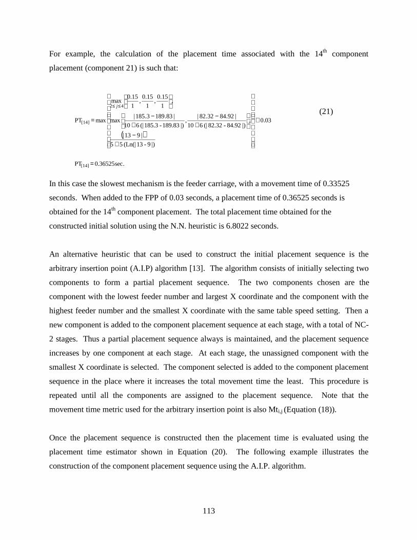
113
For example, the calculation of the placement time associated with the 14th component
placement (component 21) is such that:
( )
03.0
|)9-13(Ln(| 55
|913|
,|)84.92-82.32(| 6 10
|92.8432.82|,
|)189.83-185.3(| 6 10
|83.1893.185|max
,1
15.0,
1
15.0,
1
0.15max
max PT
42
[14] +
+−
+−
+−
=
≤≤ j(21)
.sec36525.0 PT[14] =
In this case the slowest mechanism is the feeder carriage, with a movement time of 0.33525
seconds. When added to the FPP of 0.03 seconds, a placement time of 0.36525 seconds is
obtained for the 14th component placement. The total placement time obtained for the
constructed initial solution using the N.N. heuristic is 6.8022 seconds.
An alternative heuristic that can be used to construct the initial placement sequence is the
arbitrary insertion point (A.I.P) algorithm [13]. The algorithm consists of initially selecting two
components to form a partial placement sequence. The two components chosen are the
component with the lowest feeder number and largest X coordinate and the component with the
highest feeder number and the smallest X coordinate with the same table speed setting. Then a
new component is added to the component placement sequence at each stage, with a total of NC-
2 stages. Thus a partial placement sequence always is maintained, and the placement sequence
increases by one component at each stage. At each stage, the unassigned component with the
smallest X coordinate is selected. The component selected is added to the component placement
sequence in the place where it increases the total movement time the least. This procedure is
repeated until all the components are assigned to the placement sequence. Note that the
movement time metric used for the arbitrary insertion point is also Mti,j (Equation (18)).
Once the placement sequence is constructed then the placement time is evaluated using the
placement time estimator shown in Equation (20). The following example illustrates the
construction of the component placement sequence using the A.I.P. algorithm.

114
Using the component data from Table A.2 and the initial feeder assignment from Table A.10, an
initial partial sequence is constructed. Component 1 is selected as the first component of the
partial sequence since it has the lowest feeder number and the largest X coordinate. Component
13 is selected as the end of the partial sequence since it has the highest feeder for the same table
speed setting as component 1 and has the smallest X coordinate. The movement time associated
with this partial sequence {1, 13} using the movement time matrix from Table A.11 is 0.4298
seconds. Component 17 is selected as the next component to be inserted in the partial sequence
since it has the smallest X coordinate. The next step is to decide where in the partial sequence
{1, 13} to insert component 17. There are three possibilities in this case, the partial sequence
{17, 1, 13} with a total movement time of 6055862.56 seconds, the partial sequence {1, 17, 13}
with a total movement time of 10555862.13 seconds, and the partial sequence {1, 13, 17} with a
total movement time of 4500000.43 seconds. Since the sequence {1, 13, 17} has the smallest
movement time then it becomes the new partial sequence. Note that these movement times are
calculated using the movement times from Table A.11. This process is repeated until all the
components are assigned. Table A.13 shows the initial solution and the placement times (using
Equation (20)) associated with each component placement. The total placement time for the
initial solution constructed using the A.I.P. algorithm is 6.7138 seconds.

115
Table A.13 General Optimization Initial Solution Using A.I.P. Algorithm
ComponentNumber
ComponentType
STR STS X-Location(mm)
Y-Location (mm)
Feeder Slot
PlacementTime (sec.)
1 1 0.8 0 257.9 82.38 1 0.033 1 0.8 0 226.91 171.28 1 0.21752 7 0.8 0 245.2 105.24 2 0.235 2 0.8 0 189.32 71.72 3 0.21754 2 0.8 0 187.29 82.89 3 0.236 3 1 0 257.9 84.42 4 0.192829 3 1 0 188.81 95.59 4 0.1927410 4 1 0 257.9 86.45 5 0.2662511 4 1 0 246.73 165.95 5 0.1932412 4 1 0 202.53 170.78 5 0.1906113 8 1 0 189.83 84.92 7 0.459847 8 1 0 239.61 125.56 7 0.191278 8 1 0 213.45 171.03 7 0.1907723 9 1 1 189.1 87.21 13 0.2662522 9 1 1 187.63 86.37 13 0.40521 9 1 1 185.3 82.32 13 0.40515 5 0.4 1 249.52 172.05 11 0.40519 6 0.4 1 239.11 171.28 9 0.40516 5 0.4 1 195.16 141.82 11 0.40514 5 0.4 1 243.17 90.77 11 0.40518 6 0.4 1 240.63 81.37 9 0.40520 6 0.4 1 192.37 95.59 9 0.40517 5 0.4 1 184.75 79.08 11 0.405
For this particular example, the N.N. algorithm yields a placement time of 6.8022 seconds,
which is slightly higher placement time of the A.I.P. algorithm (6.7138 seconds). The difference
in the placement times is 0.0884 seconds.
General Optimization Improvement of Initial Solution Example
In order to explain the improvement procedure, the initial solution constructed using the A.I.P.
algorithm in step 5 is further improved using the two reverse algorithm. The two reverse
algorithm is applied to the placement sequence while the feeder assignment remains fixed, and
then applied to the feeder assignment while the placement sequence remains fixed.

116
In order to use the two reverse algorithm [18] an initial component placement sequence and
feeder assignment must exist and the component placement time must be known. The two
reverse algorithm [18] works as follows: A sequence is represented as a set of ordered nodes
such as: 5, 2, 3, 4, 7, 8, 9, 1, 6,. . . , n. Then, part of the sequence starting from position i in the
sequence and ending at position j in the sequence is reversed. For example if i = 3 and j = 8 the
partial sequence starting from position 3 and ending at position 8 is reversed such that the new
sequence (placement or feeder sequence) tour is: 5, 2, 1, 9, 8, 7, 4, 3, 6,. . . ,n. The values of i
and j are chosen systematically. Initially i = 1 and j = i + 1 and a partial sequence from i to j is
reversed and the new component placement time is calculated. If the component placement time
is reduced, then the new sequence is kept and i = 1, j = i + 1 and the component placement time
is updated. Otherwise the previous sequence is kept and j = j +1. If j reaches the last position in
the sequence then i = i + 1 and j = i + 1. If i reaches the last position in the sequence then the
algorithm stops. Note that the two reverse algorithm changes either the placement sequence or
the feeder sequence while the other one is held fixed. In the case of the placement sequence the
two reverse algorithm stops when i = total number of components (NC). In the case of the feeder
sequence the algorithm stops when i = total number of component types.
In order to illustrate the use of the two reverse algorithm the initial placement sequence shown in
Table A.13 is used.
Step 6: Use the two reverse algorithm to improve the component placement sequence and hold
the feeder assignment fix.
The component placement sequence from Table A.13 is {1, 3, 2, 5, 4, 6, 9, 10, 11, 12, 13, 7, 8,
23, 22, 21, 15, 19, 16, 14, 18, 20, 17} with an associated component placement time of 6.7138
seconds. Starting with i = 1 and j = 2 and reversing the partial sequence, the placement sequence
{3, 1, 2, 5, 4, 6, 9, 10, 11, 12, 13, 7, 8, 23, 22, 21, 15, 19, 16, 14, 18, 20, 17} is obtained. The
placement time for this sequence is 6.7138 seconds. Since the placement time is not reduced
compared to the current best sequence, the proposed placement sequence is not accepted and j =
3. The next proposed sequence {2, 3, 1, 5, 4, 6, 9, 10, 11, 12, 13, 7, 8, 23, 22, 21, 15, 19, 16, 14,
18, 20, 17} is obtained by reversing the partial sequence starting in position i = 1 and ending in

117
position j = 3. The placement time the proposed sequence is 6.7138 seconds. Since the
placement time is not reduced, the proposed sequence is not accepted and j = 4. The procedure is
repeated until i reaches 23. The final placement time obtained is 6.7010, which is 0.0128
seconds less than the initial solution constructed with the A.I.P algorithm. Even though the
improvement does not seem to be significant, much better improvements are obtained for
problems with larger number of components as shown in the industrial case study presented in
Chapter VI. Table A.14 shows the solution obtained after using the two reverse algorithm to
improve the placement sequence.
Table A.14 General Optimization Improved Placement Sequence Solution
Component Number
ComponentType
STR STS X-Location(mm)
Y-Location (mm)
Feeder Slot
PlacementTime (sec.)
1 1 0.8 0 257.9 82.38 1 0.0311 1 0.8 0 226.91 171.28 1 0.21756 7 0.8 0 245.2 105.24 2 0.2317 2 0.8 0 189.32 71.72 3 0.217521 2 0.8 0 187.29 82.89 3 0.2319 3 1 0 188.81 95.59 4 0.182 3 1 0 257.9 84.42 4 0.1927413 4 1 0 257.9 86.45 5 0.2662465 4 1 0 246.73 165.95 5 0.19324413 4 1 0 202.53 170.78 5 0.1906116 8 1 0 189.83 84.92 7 0.4598369 8 1 0 239.61 125.56 7 0.19126712 8 1 0 213.45 171.03 7 0.19077418 9 1 1 189.1 87.21 13 0.26624620 9 1 1 187.63 86.37 13 0.40522 9 1 1 185.3 82.32 13 0.4054 5 0.4 1 249.52 172.05 11 0.40510 6 0.4 1 239.11 171.28 9 0.40514 5 0.4 1 195.16 141.82 11 0.4057 5 0.4 1 243.17 90.77 11 0.4058 6 0.4 1 240.63 81.37 9 0.40515 6 0.4 1 192.37 95.59 9 0.40523 5 0.4 1 184.75 79.08 11 0.405
The next step of the improvement procedure consists of applying the two reverse algorithm to
the feeder sequence.
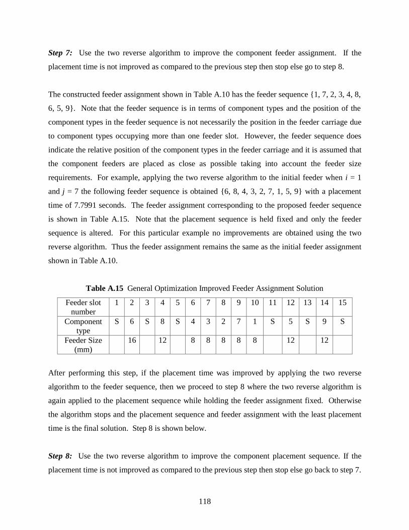
118
Step 7: Use the two reverse algorithm to improve the component feeder assignment. If the
placement time is not improved as compared to the previous step then stop else go to step 8.
The constructed feeder assignment shown in Table A.10 has the feeder sequence {1, 7, 2, 3, 4, 8,
6, 5, 9}. Note that the feeder sequence is in terms of component types and the position of the
component types in the feeder sequence is not necessarily the position in the feeder carriage due
to component types occupying more than one feeder slot. However, the feeder sequence does
indicate the relative position of the component types in the feeder carriage and it is assumed that
the component feeders are placed as close as possible taking into account the feeder size
requirements. For example, applying the two reverse algorithm to the initial feeder when i = 1
and j = 7 the following feeder sequence is obtained {6, 8, 4, 3, 2, 7, 1, 5, 9} with a placement
time of 7.7991 seconds. The feeder assignment corresponding to the proposed feeder sequence
is shown in Table A.15. Note that the placement sequence is held fixed and only the feeder
sequence is altered. For this particular example no improvements are obtained using the two
reverse algorithm. Thus the feeder assignment remains the same as the initial feeder assignment
shown in Table A.10.
Table A.15 General Optimization Improved Feeder Assignment Solution
Feeder slotnumber
1 2 3 4 5 6 7 8 9 10 11 12 13 14 15
Componenttype
S 6 S 8 S 4 3 2 7 1 S 5 S 9 S
Feeder Size(mm)
16 12 8 8 8 8 8 12 12
After performing this step, if the placement time was improved by applying the two reverse
algorithm to the feeder sequence, then we proceed to step 8 where the two reverse algorithm is
again applied to the placement sequence while holding the feeder assignment fixed. Otherwise
the algorithm stops and the placement sequence and feeder assignment with the least placement
time is the final solution. Step 8 is shown below.
Step 8: Use the two reverse algorithm to improve the component placement sequence. If the
placement time is not improved as compared to the previous step then stop else go back to step 7.

119
APPENDIX B
FIXED SETUP OPTIMIZATION SOLUTION APPROACH
EXAMPLE
Initial Solution Construction Example
In order to explain the initial solution construction procedure, a detailed example is presented.
The data necessary to present the example includes machine data and PCB component data. The
machine data includes:
• the PCB table velocity functions for each table speed setting,
• the feeder carriage velocity function,
• the minimum turret rotation time (MTR),
• the fixed pick and place time (FPP),
• the number of placement heads in the turret, and
• the feeder slots capacity of the machine.
The PCB component data includes:
• the number of components to be mounted,
• the component number designated to each component,
• the component type associated with each component,
• the STR associated with each component type,
• the STS associated with each component type,
• the feeder size associated with each component type,
• the X and Y coordinates associated with each component on the PCB, and
• the feeder slot locations associated with the component types included in the fixed
setup.
Tables B.1, B2 and B.3 show all the necessary machine and PCB component data.

120
Table B.1 Fixed Setup Optimization Machine Data
Number of Heads (NH) 6Number of Feeder Slots 19Minimum Turret Rotation Time (MRT) 0.15Fixed Pick and Place Time (FPP) 0.03High PCB Table Speed Setting (0) Velocity FunctionX-direction (mm/sec.)
Vx[0] = 10 + 6 (|X[i] -X[i-1] |)
High PCB Table Speed Setting (0) Velocity FunctionY-direction (mm/sec.)
Vy[0] = 10 + 6 (|Y[i] -Y[i-1] |)
Low PCB Table Speed Setting (1) Velocity FunctionX-direction (mm/sec.)
Vx[1] = 7 + 3 (|X[i] -X[i-1] |)
Low PCB Table Speed Setting (1) Velocity FunctionY-direction (mm/sec.)
Vy[1] = 7 + 3 (|Y[i] -Y[i-1] |)
Feeder Carriage Velocity Function (slots/sec.) Vfc = 5+5 (Ln(|FS[j] -FS[j-1] |))
Table B.2 Fixed Setup Optimization Component Data
ComponentNumber
ComponentType
STR STS Feeder Size(mm)
X-Location(mm)
Y-Location(mm)
1 1 0.8 0 8 257.9 82.382 7 0.8 0 8 245.2 105.243 1 0.8 0 8 226.91 171.284 2 0.8 0 8 187.29 82.895 2 0.8 0 8 189.32 71.726 3 1 0 8 257.9 84.427 8 1 0 12 239.61 125.568 8 1 0 12 213.45 171.039 3 1 0 8 188.81 95.5910 4 1 0 8 257.9 86.4511 4 1 0 8 246.73 165.9512 4 1 0 8 202.53 170.7813 8 1 0 12 189.83 84.9214 5 0.4 1 12 243.17 90.7715 5 0.4 1 12 249.52 172.0516 5 0.4 1 12 195.16 141.8217 5 0.4 1 12 184.75 79.0818 6 0.4 1 16 240.63 81.3719 6 0.4 1 16 239.11 171.2820 6 0.4 1 16 192.37 95.5921 9 1 1 12 185.3 82.3222 9 1 1 12 187.63 86.3723 9 1 1 12 189.1 87.21

121
Table B.3 Fixed Setup Component Data
Component Type Feeder Size (mm) Fixed Setup2 8 Feeder Slot 28 12 Feeder Slot 79 12 Feeder Slot 910 8 Feeder Slot 511 16 Feeder Slot 1112 8 Feeder Slot 3
Table B.3 shows all the component types included in the fixed setup. Note this table includes all
fixed component types, both those on the PCB and those on other PCBs in the fixed setup. Table
B.4 shows the initial status of the feeder carriage.
Table B.4 Fixed Setup Optimization Initial Feeder Carriage Status
Feederslot number
1 2 3 4 5 6 7 8 9 10 11 12 13 14 15 16 17 18 19
Component Type
2 12 10 S 8 S S 11 S 9
FeederSize (mm)
8 8 8 16 16 8
Step 1: Devide the set of NC = 23 components into G groups, each having the same
specification PCB table speed setting (STS) and same specification turret rotation rate (STR). In
this case since there are two different STSs, each having two different STRs, then G equals four.
The groups are formed by the following components:
• Group 1, STS = 0 and STR = 1, component number {1, 2, 3, 4, 5}.
• Group 2, STS = 0 and STR = 0.8, component number {6, 7, 8, 9, 10, 11, 12, 13}.
• Group 3, STS = 1 and STR = 0.4, component number {13, 14, 15, 16, 17, 18, 19, 20}.
• Group 4, STS = 1 and STR = 1, component number {21, 22, 23}.
Step 2: For each group G, construct an initial component placement sequence that minimizes the
PCB table movement time (ttb) using the nearest neighbor (N.N.) algorithm [13] starting with the
component with the smallest X coordinate. A PCB table movement time matrix, representing the
time to move between two specific components is calculated for each group. The PCB table
movement time matrix (Table B.5) is calculated for the components in Group 1 using the ttb

122
metric from Equation (2) and substituting Vx[S] and Vy[S] with their corresponding functions
shown in Table B.2. Note that the units associated with the body of Table B.5 are in seconds.
Table B.5 Fixed Setup Optimization Group 1 PCB Table Movement Time Matrix
From Component -To Component
1 2 3 4 5
1 0 0.155341 0.1636 0.162823 0.1627122 0.155341 0 0.162564 0.162004 0.161843 0.1636 0.162564 0 0.163582 0.1639234 0.162823 0.162004 0.163582 0 0.1450275 0.162712 0.16184 0.163923 0.145027 0
After determining the PCB table movement time between all the components in the group, the
component number with the lowest X coordinate is chosen as the starting point for the N.N.
algorithm. The N.N. algorithm consists of starting with one component number and then finding
its nearest neighbor (another component) based on the calculated PCB table movement time
matrix and assigning that nearest neighbor next in the placement sequence [13]. For group 1,
component 4 is selected as the starting point since it has the lowest X coordinate (187.29 mm).
The nearest neighbor algorithm is then applied and component 5 is selected as the next
component in the sequence. This procedure is repeated until all components in the group are
assigned to the placement sequence, resulting in the following sequence {4, 5, 2, 1, 3}. The
procedure is repeated for each group. Table B.6 shows the resulting placement sequence for
each group.
Table B.6 Fixed Setup Optimization Group Placement Sequences
Group 1 Component Number: 4, 5, 2, 1, 3Component Type : 2, 2, 7, 1, 1
Group 2 Component Number: 9, 13, 7, 10, 6, 11, 8, 12Component Type : 3, 8 , 8, 4 , 3, 4, 8, 4
Group 3 Component Number: 17, 20, 16, 19, 15, 14 , 18Component Type : 5 , 6 , 5, 6, 5, 5, 6
Group 3 Component Number: 21, 22, 23Component Type : 9 , 9, 9
Step 3: For each group G, construct a component type flow matrix using the placement
sequences generated in Step 3. If component type i is placed after component type j then the

123
flow between component types i and j and component types j and i is increased by one. Note
that the flow between component types i and j is denoted by Fij . If i and j are the same
component type then Fij is equal to zero.
The component type flow matrix for group 1 is formed by the flows between component types 1,
2 and 7. The component type flow matrix for group 1 is calculated using the placement sequence
for group 1 in terms of component types {2, 2, 7, 1, 1} as shown in Table B.6. It can be
observed that there is one movement from component type 2 to component type 7 and one
movement from component type 7 to component type 1. Note that the flows between identical
component types are not counted. Therefore, the movement form component type 2 (component
number 4) to component type 2 (component number 5) and from component type 1 (component
number 1) to component type 1 (component number 3) are not counted and their flows are set
equal to zero (F11 = 0, F22 = 0). The remaining component type flows for group 1 are as follows:
F12 = F21 = 0, F17 = F71 = 1, F27 = F72 = 1. Tables B.7 to B.10 show the component type flow
matrix for each group, where the headers of the columns and rows in the tables are the
component types.
Table B.7 Fixed Setup Optimization Group 1 Component Type Flow Matrix
From-ToComponent Type
1 2 7
1 0 0 12 0 0 17 1 1 0
Table B.8 Fixed Setup Optimization Group 2 Component Type Flow Matrix
From-ToComponent Type 3 4 8
3 0 2 14 2 0 38 1 3 0

124
Table B.9 Fixed Setup Optimization Group 3 Component Type Flow Matrix
From-ToComponent Type 5 6
5 0 56 5 0
Table B.10 Fixed Setup Optimization Group 3 Component Type Flow Matrix
From-ToComponent Type
9
9 0
Step 4: For each group G, an initial feeder assignment that minimizes the feeder carriage
movement time (tfc) is constructed using a greedy algorithm. Note that the only component types
to be assigned are the component types not included in the fixed setup. Start with the group with
the smallest STS (fastest table speed setting) and smallest STR (slowest turret rate) taking into
account the feeder space required by each component type. The greedy algorithm consists of the
following steps:
• Step 4.1: The first step consists of setting the flow between all the assigned components
equal to –1. In addition, count the number of assigned component types and the number of
unassigned component types. Note that initially the number of assigned component types
equals the number of fixed setup component types in the group. Once the number of
assigned and unassigned component types is identified three possible cases exist. In the first
case, the number of assigned component types is greater than 0 and the number of unassigned
component types is equal to 0. For this case no component types need to be assigned, thus
we proceed to the next group. The second case is when the number of assigned component
types is greater than 0 and the number of unassigned component types is also greater than 0.
If this is the case, then go to step 4.2. For the third case, the number of assigned component
types is equal to 0 and the number of unassigned component types is greater than 0. For this
case, go to step 4.3.
• Step 4.2: Select the assigned component type and unassigned component type with the
maximum flow in the component type matrix. Check if the selected unassigned component

125
type can be assigned in the feeder carriage immediately to the left of the selected assigned
component type. If it cannot, check if it can be assigned immediately to the right of the
assigned component type selected. In the case that the unassigned component type selected
cannot be assigned either on the left or on the right, the flow between the assigned
component type selected and the unassigned component type selected is set equal to –1. This
is done to avoid repeating this step with the same assigned and unassigned component types.
Note that the flow between the unassigned component type selected and the assigned type
selected is not set to –1, this flow maybe used in step 4.3. In case that the unassigned
component type selected can be assigned to either the immediate left or right of the assigned
component type selected, then it is assigned to the feeder carriage, and the flow between all
assigned component types is reset to –1. This Step is repeated until the flow between all the
assigned component types and the unassigned component types is equal to –1. If all the
component types in the group have been assigned then go back to step 4.1 and start with the
next group of components, otherwise go to step 4.3.
An important fact to notice is that a flow of –1 between an assigned component type and an
unassigned component type indicates that the unassigned component type could not be assigned
immediately next to the assigned component type in the feeder carriage.
• Step 4.3: Since no more free feeder slots with enough capacity could be found immediately
next to the assigned component types in the group, then the unassigned component type with
the highest flow with any of the component types in the group is selected to be assigned next.
The unassigned component type is assigned to the closest feeder slot available either to the
left or to the right of the assigned component type in the group located most to the left in the
feeder carriage. If there are two closest feeder slots available, the feeder slot to the left is
selected to break the tie. Once the unassigned type number is assigned, the flow between all
assigned components is reset to –1. If all the component types in the group have been
assigned go back to step 4.1 and start with the next group of components, otherwise go back
to step 4.2.

126
• Step 4.4: This step is only used when there are no assigned component types in the group
and no point of reference exists in order to assign the unassigned component types to the
feeder carriage. The procedure consists of identifying the feeder slot associated with the
right-most assigned component type included in the PCB with the same STS and nearest
higher STR to the STR of the group being assigned. Once the feeder slot number has been
identified, the component type with the maximum flow with any of the unassigned
component types in the group is assigned to the closest location to the right of the feeder slot
selected. If there are no feeder slots available to the right of the feeder slot selected and the
end of the feeder carriage, the unassigned component type is assigned to the closest feeder
slot location to the left of the feeder slot selected. If the group being assigned is the first
group or no other component types with the same table speed and a lower turret rate are
found, then the first component is assigned to the first feeder slot available in the feeder
carriage starting from the left. If any unassigned components are left after assigning the first
component go back to step 4.2, else proceed to the next group, or if all the groups have been
assigned, stop.
The following example illustrates the construction of the initial feeder assignment using the
procedure explained in step 4.
Starting with group 1 and step 4.1 it can be observed from Table B.3 that component type 2 is
included in the fixed setup and component types 1 and 7 are unassigned, therefore we continue to
step 4.2. In step 4.2 the component type with the highest flow with the assigned component
types is selected. In this case the unassigned component type having the highest flow with
component type 2 (the assigned one) is component type 7. Once component type 7 is selected
we check if it can be assigned to the feeder slot immediately to the right of component type 2,
which is feeder slot 1. From Table B.4 it can be observed that feeder slot 1 is free, thus
component type 7 is assigned to slot 1. After assigning component type 7 to slot 1 the
component type flow between all assigned component types in the group is reset to –1. The
updated component type flow matrix and feeder carriage status are shown in Table B.11 and
Table B.12 respectively.

127
Table B.11 Fixed Setup Optimization Group 1 Updated Component Type Flow Matrix 1
From-To ComponentType Number 1 2 7
1 0 0 12 0 0 -17 1 -1 0
Table B.12 Fixed Setup Optimization Updated Feeder Carriage Status 1
Feeder slotnumber
1 2 3 4 5 6 7 8 9 10 11 12 13 14 15 16 17 18 19
Componenttype
7 2 12 10 S 8 S S 11 S 9
Feeder Size(mm)
8 8 8 8 12 16 8
Because not all the flows between the assigned types and the unassigned component types in the
group equal to -1, step 4.2 is performed again. In this case the only unassigned component type
remaining in the group is component type 1 which has its highest flow with component type 7.
Thus, we attempt to assign it either immediately to the left or the right of the feeder slot
associated with component type 7. However, since there are no feeder slots available next to
component type 7, the flow between component type 7 and component type 1 is set equal to –1.
The updated component type flow matrix is shown in Table B.13. Note that the flow between
component type 1 and component type 7 remains the same.
Table B.13 Fixed Setup Optimization Group 1 Updated Component Type Flow Matrix 2
From-To ComponentType Number
1 2 7
1 0 0 12 0 0 -17 -1 -1 0
Since not all the flows between the assigned component types and the unassigned component
types equal to –1, repeat step 4.2 again. From Table B.13 the assigned component type and
unassigned component type with the highest flow are component type 2 and component type 1,
respectively. The flow between them is 0, which still not equal to –1. An attempt to assign
component type 1 next to component type 2 is made. However, since there are no available
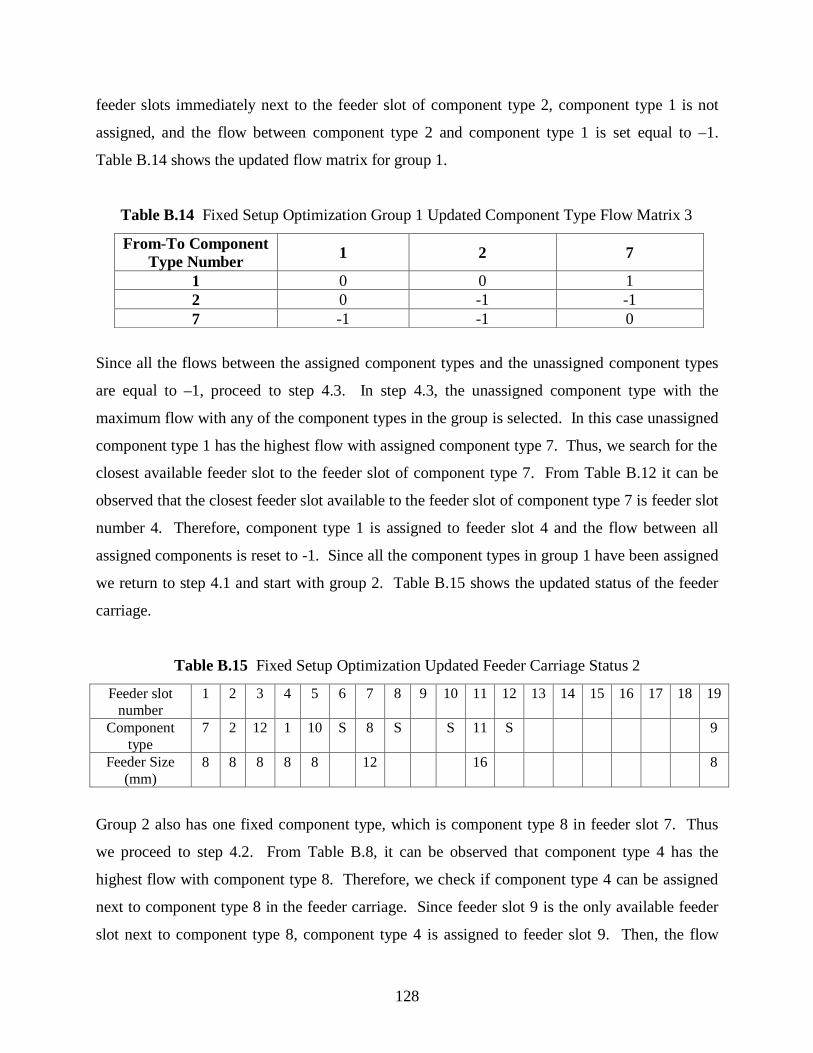
128
feeder slots immediately next to the feeder slot of component type 2, component type 1 is not
assigned, and the flow between component type 2 and component type 1 is set equal to –1.
Table B.14 shows the updated flow matrix for group 1.
Table B.14 Fixed Setup Optimization Group 1 Updated Component Type Flow Matrix 3
From-To ComponentType Number 1 2 7
1 0 0 12 0 -1 -17 -1 -1 0
Since all the flows between the assigned component types and the unassigned component types
are equal to –1, proceed to step 4.3. In step 4.3, the unassigned component type with the
maximum flow with any of the component types in the group is selected. In this case unassigned
component type 1 has the highest flow with assigned component type 7. Thus, we search for the
closest available feeder slot to the feeder slot of component type 7. From Table B.12 it can be
observed that the closest feeder slot available to the feeder slot of component type 7 is feeder slot
number 4. Therefore, component type 1 is assigned to feeder slot 4 and the flow between all
assigned components is reset to -1. Since all the component types in group 1 have been assigned
we return to step 4.1 and start with group 2. Table B.15 shows the updated status of the feeder
carriage.
Table B.15 Fixed Setup Optimization Updated Feeder Carriage Status 2
Feeder slotnumber
1 2 3 4 5 6 7 8 9 10 11 12 13 14 15 16 17 18 19
Componenttype
7 2 12 1 10 S 8 S S 11 S 9
Feeder Size(mm)
8 8 8 8 8 12 16 8
Group 2 also has one fixed component type, which is component type 8 in feeder slot 7. Thus
we proceed to step 4.2. From Table B.8, it can be observed that component type 4 has the
highest flow with component type 8. Therefore, we check if component type 4 can be assigned
next to component type 8 in the feeder carriage. Since feeder slot 9 is the only available feeder
slot next to component type 8, component type 4 is assigned to feeder slot 9. Then, the flow

129
between all assigned component types in group 2 is reset to –1. Table B.16 shows the updated
flow matrix and Table B.17 shows the updated feeder carriage assignment.
Table B.16 Fixed Setup Optimization Group 2 Updated Component Type Flow Matrix 1
From-To ComponentType Number 3 4 8
3 0 2 14 2 0 -18 1 -1 0
Table B.17 Fixed Setup Optimization Updated Feeder Carriage Status 3
Feeder slotnumber
1 2 3 4 5 6 7 8 9 10 11 12 13 14 15 16 17 18 19
Componenttype
7 2 12 1 10 S 8 S 4 S 11 S 9
Feeder Size(mm)
8 8 8 8 8 12 8 16 8
Since not all the flows between the assigned component types and unassigned components types
in group 2 are equal to –1, step 4.2 is repeated. This step is repeated twice in an attempt to
assign component type 3 next to the assigned component types. However, since neither
component type 4 nor component type 8 have feeder a slots available next to them, component
type 3 is not assigned and we continue to step 4.3. The updated component type flow matrix is
shown in Table B.18.
Table B.18 Fixed Setup Optimization Group 2 Updated Component Type Flow Matrix 2
From-To ComponentType Number
3 4 8
3 0 2 14 -1 0 -18 -1 -1 0
In step 4.3, the unassigned component type with the maximum flow with any of the component
types in the group is selected. In this case unassigned component type 3 has the highest flow
with assigned component type 4. The closest feeder slot available to the feeder slot of
component type 4 is feeder slot 13 as shown in Table B.17. Thus, component type 3 is assigned

130
to feeder slot number 13 and the flow between all assigned component types is reset to –1. Since
all the components on group 2 have been assigned, group 3 is assigned next. Table B.19 shows
the updated feeder carriage assignment.
Table B.19 Fixed Setup Optimization Updated Feeder Carriage Status 4
Feeder slotnumber
1 2 3 4 5 6 7 8 9 10 11 12 13 14 15 16 17 18 19
Componenttype
7 2 12 1 10 S 8 S 4 S 11 S 3 9
Feeder Size(mm)
8 8 8 8 8 12 8 16 8 8
Group 3, has no assigned (fixed setup) component types, thus step 4.4 is performed next. Since
there are no component types having the same table speed as group 3 assigned in the feeder
carriage, the first feeder slot available from the left of the feeder carriage is selected for the next
component type to be assigned. Component type 5 and component type 6 have the highest flow
in the component type flow matrix for group 3 (Table B.24). However, since component type 5
is located more towards the left in the component type flow matrix, it is assigned first. Note that
this is an arbitrary rule to decide which of the two component types with the highest flow is
assigned to the feeder carriage first. In this case, the first available slot from the left of the feeder
carriage is feeder slot 14. However, since the feeder size of component type 5 is 12 mm it does
not fit in slot 14, therefore it is assigned to the next available feeder slot, which is feeder slot 15.
Table B.20 shows the updated feeder carriage assignment.
Table B.20 Fixed Setup Optimization Updated Feeder Carriage Status 5
Feeder slotnumber
1 2 3 4 5 6 7 8 9 10 11 12 13 14 15 16 17 18 19
Componenttype
7 2 12 1 10 S 8 S 4 S 11 S 3 S 5 S 9
Feeder Size(mm)
8 8 8 8 8 12 8 16 8 12 8
Because there is still one component type unassigned in group 3 step 4.2 is performed.
Component type 6 is the only unassigned component type in group 3, and it has the highest flow
with component type 5. Thus, component type 6 is assigned to feeder slot 17, which is next to
the feeder slot of component type 5. Note that if there was no component type assigned to feeder
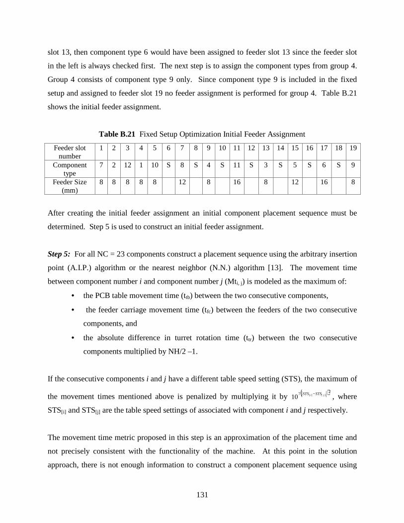
131
slot 13, then component type 6 would have been assigned to feeder slot 13 since the feeder slot
in the left is always checked first. The next step is to assign the component types from group 4.
Group 4 consists of component type 9 only. Since component type 9 is included in the fixed
setup and assigned to feeder slot 19 no feeder assignment is performed for group 4. Table B.21
shows the initial feeder assignment.
Table B.21 Fixed Setup Optimization Initial Feeder Assignment
Feeder slotnumber
1 2 3 4 5 6 7 8 9 10 11 12 13 14 15 16 17 18 19
Componenttype
7 2 12 1 10 S 8 S 4 S 11 S 3 S 5 S 6 S 9
Feeder Size(mm)
8 8 8 8 8 12 8 16 8 12 16 8
After creating the initial feeder assignment an initial component placement sequence must be
determined. Step 5 is used to construct an initial feeder assignment.
Step 5: For all NC = 23 components construct a placement sequence using the arbitrary insertion
point (A.I.P.) algorithm or the nearest neighbor (N.N.) algorithm [13]. The movement time
between component number i and component number j (Mti, j) is modeled as the maximum of:
• the PCB table movement time (ttb) between the two consecutive components,
• the feeder carriage movement time (tfc) between the feeders of the two consecutive
components, and
• the absolute difference in turret rotation time (ttr) between the two consecutive
components multiplied by NH/2 –1.
If the consecutive components i and j have a different table speed setting (STS), the maximum of
the movement times mentioned above is penalized by multiplying it by ( )27 ][][10 ji STSSTS − , where
STS[i] and STS[j] are the table speed settings of associated with component i and j respectively.
The movement time metric proposed in this step is an approximation of the placement time and
not precisely consistent with the functionality of the machine. At this point in the solution
approach, there is not enough information to construct a component placement sequence using

132
the true component placement time estimator function due to the multiple heads in the turret.
The proposed metric provides a way of penalizing PCB table movements, feeder carriage
movements that are incurred throughout the placement of the components, changes in the turret
rotation rate (STR), and changes in the PCB table speed setting (STS). This modified movement
time metric can be used in combination with a heuristic to construct a placement sequence. For
this step of the construction heuristic, after substituting Vx[0], Vy[0], Vx[1], Vy[1] , and Vfc with the
appropriate functions, the movement time between components i and j is as follows:
+−
−−
−=
|))FS-FS(Ln(| 55
|FSFS|,
V
|yy|,
V
|xx|max,
.sec15.0sec. 0.152max)(
[j][i]
[j]][
Y[STS[i]]
][][
X[STS[i]]
][][
][][,
ijiji
jiji
STRSTRMt α (22)
where:
α = 1 if STS[i] = STS, otherwise α = ( )27 ][][10 ji STSSTS −
,
Vx[0] = 10 + 6 (|X[i] -X[i-1] |),
Vy[0] = 10 + 6 (|Y[i] -Y[i-1] |),
Vx[1] = 7 + 3 (|X[i] -X[i-1] |), and
Vy[1] = 7 + 3 (|Y[i] -Y[i-1] |).
Table B.22 shows the Mti,j matrix. Note that this matrix is calculated using Equation
(22). The components in the matrix are arranged in descending order of X coordinate.

133
Table B.22 Fixed Setup Optimization Mti,j Matrix
Comp. 1 6 10 15 11 2 14 18 71 0 0.562988291 0.383224293 6474596.253 0.383224293 0.285903215 6474596.253 7293231.234 0.285903215
6 0.562988291 0 0.335247827 4500000 0.335247827 0.688684157 4500000 4500000 0.429836457
10 0.383224293 0.335247827 0 4500000 0.163244353 0.519574728 4500000 4500000 0.236246444
15 6474596.253 4500000 4500000 0 4500000 7694300.327 0.324031255 0.32497133 4500000
11 0.383224293 0.335247827 0.163244353 4500000 0 0.519574728 4500000 4500000 0.236246444
2 0.285903215 0.688684157 0.519574728 7694300.327 0.519574728 0 7694300.327 8482239.215 0.429836457
14 6474596.253 4500000 4500000 0.324031255 4500000 7694300.327 0 0.267045455 4500000
18 7293231.234 4500000 4500000 0.32497133 4500000 8482239.215 0.267045455 0 6055862.131
7 0.285903215 0.429836457 0.236246444 4500000 0.236246444 0.429836457 4500000 6055862.131 0
19 7293231.234 4500000 4500000 0.272299241 4500000 8482239.215 0.323944795 0.324901529 6055862.131
3 0.163599558 0.562988291 0.383224293 6474596.253 0.383224293 0.285903215 6474596.253 7293231.234 0.285903215
8 0.285903215 0.429836457 0.236246444 4500000 0.236246444 0.429836457 4500000 6055862.131 0.160773637
12 0.383224293 0.335247827 0.163436567 4500000 0.160610465 0.519574728 4500000 4500000 0.236246444
16 6474596.253 4500000 4500000 0.319614299 4500000 7694300.327 0.318763659 0.320945049 4500000
20 7293231.234 4500000 4500000 0.323462222 4500000 8482239.215 0.318695107 0.317960206 6055862.131
13 0.285903215 0.429836457 0.236246444 4500000 0.236246444 0.429836457 4500000 6055862.131 0.161267332
5 0.236246444 0.647459625 0.475235132 7293231.234 0.475235132 0.2 7293231.234 8090505.353 0.383224293
23 8090505.353 4298364.573 6055862.131 0.45 6055862.131 9253614.369 0.45 0.45 6886841.575
9 0.562988291 0.162740849 0.335247827 4500000 0.335247827 0.688684157 4500000 4500000 0.429836457
22 8090505.353 4298364.573 6055862.131 0.45 6055862.131 9253614.369 0.45 0.45 6886841.575
4 0.236246444 0.647459625 0.475235132 7293231.234 0.475235132 0.2 7293231.234 8090505.353 0.383224293
21 8090505.353 4298364.573 6055862.131 0.45 6055862.131 9253614.369 0.45 0.45 6886841.575
17 6474596.253 4500000 4500000 0.325172257 4500000 7694300.327 0.320531109 0.319972515 4500000
Comp. 19 3 8 12 16 20 13 5 231 7293231.234 0.163599558 0.285903215 0.383224293 6474596.253 7293231.234 0.285903215 0.236246444 8090505.353
6 4500000 0.562988291 0.429836457 0.335247827 4500000 4500000 0.429836457 0.647459625 4298364.573
10 4500000 0.383224293 0.236246444 0.163436567 4500000 4500000 0.236246444 0.475235132 6055862.131
15 0.272299241 6474596.253 4500000 4500000 0.319614299 0.323462222 4500000 7293231.234 0.45
11 4500000 0.383224293 0.236246444 0.160610465 4500000 4500000 0.236246444 0.475235132 6055862.131
2 8482239.215 0.285903215 0.429836457 0.519574728 7694300.327 8482239.215 0.429836457 0.2 9253614.369
14 0.323944795 6474596.253 4500000 4500000 0.318763659 0.318695107 4500000 7293231.234 0.45
18 0.324901529 7293231.234 6055862.131 4500000 0.320945049 0.317960206 6055862.131 8090505.353 0.45
7 6055862.131 0.285903215 0.160773637 0.236246444 4500000 6055862.131 0.161267332 0.383224293 6886841.575
19 0 7293231.234 6055862.131 4500000 0.316528628 0.323364805 6055862.131 8090505.353 0.45
3 7293231.234 0 0.285903215 0.383224293 6474596.253 7293231.234 0.285903215 0.236246444 8090505.353
8 6055862.131 0.285903215 0 0.236246444 4500000 6055862.131 0.16350207 0.383224293 6886841.575
12 4500000 0.383224293 0.236246444 0 4500000 4500000 0.236246444 0.475235132 6055862.131
16 0.316528628 6474596.253 4500000 4500000 0 0.317317592 4500000 7293231.234 0.45
20 0.323364805 7293231.234 6055862.131 4500000 0.317317592 0 6055862.131 8090505.353 0.45
13 6055862.131 0.285903215 0.16350207 0.236246444 4500000 6055862.131 0 0.383224293 6886841.575
5 8090505.353 0.236246444 0.383224293 0.475235132 7293231.234 8090505.353 0.383224293 0 8869842.857
23 0.45 8090505.353 6886841.575 6055862.131 0.45 0.45 6886841.575 8869842.857 0
9 4500000 0.562988291 0.429836457 0.335247827 4500000 4500000 0.429836457 0.647459625 4298364.573
22 0.45 8090505.353 6886841.575 6055862.131 0.45 0.45 6886841.575 8869842.857 0.128834356
4 8090505.353 0.236246444 0.383224293 0.475235132 7293231.234 8090505.353 0.383224293 0.145027266 8869842.857
21 0.45 8090505.353 6886841.575 6055862.131 0.45 0.45 6886841.575 8869842.857 0.225657591
17 0.325105783 6474596.253 4500000 4500000 0.321381006 0.292057315 4500000 7293231.234 0.45

134
Table B.22 Fixed Setup Optimization Mti,j Matrix
Comp. 9 22 4 21 171 0.562988291 8090505.353 0.236246444 8090505.353 6474596.253
6 0.162740849 4298364.573 0.647459625 4298364.573 4500000
10 0.335247827 6055862.131 0.475235132 6055862.131 4500000
15 4500000 0.45 7293231.234 0.45 0.325172257
11 0.335247827 6055862.131 0.475235132 6055862.131 4500000
2 0.688684157 9253614.369 0.2 9253614.369 7694300.327
14 4500000 0.45 7293231.234 0.45 0.320531109
18 4500000 0.45 8090505.353 0.45 0.319972515
7 0.429836457 6886841.575 0.383224293 6886841.575 4500000
19 4500000 0.45 8090505.353 0.45 0.325105783
3 0.562988291 8090505.353 0.236246444 8090505.353 6474596.253
8 0.429836457 6886841.575 0.383224293 6886841.575 4500000
12 0.335247827 6055862.131 0.475235132 6055862.131 4500000
16 4500000 0.45 7293231.234 0.45 0.321381006
20 4500000 0.45 8090505.353 0.45 0.292057315
13 0.429836457 6886841.575 0.383224293 6886841.575 4500000
5 0.647459625 8869842.857 0.145027266 8869842.857 7293231.234
23 4298364.573 0.128834356 8869842.857 0.225657591 0.45
9 0 4298364.573 0.647459625 4298364.573 4500000
22 4298364.573 0 8869842.857 0.211488251 0.45
4 0.647459625 8869842.857 0 8869842.857 7293231.234
21 4298364.573 0.211488251 8869842.857 0 0.45
17 4500000 0.45 7293231.234 0.45 0
After constructing the Mtij movement time matrix, two alternative heuristics can be used to
construct an initial component placement sequence. These are the nearest neighbor heuristic
(N.N.) and the arbitrary insertion point heuristic (A.I.P) [13]. In the case of the nearest neighbor
heuristic the component with the smallest STS, lowest feeder number and smallest X coordinate
is selected as the starting component number for the placement sequence.
The N.N. algorithm [13] is used to create the initial placement sequence in the same manner it is
applied in the general optimization solution approach. For this example component number 2 is
selected as the starting component since it has the lowest STS, lowest feeder number and
smallest X coordinate. Then the N.N. algorithm is applied using the Mtij movement time matrix
to obtain the movement time between any two components. Table B.23 shows the initial
solution obtained using the N.N. algorithm to construct the initial placement sequence.

135
Table B.23 Fixed Setup Optimization Initial Solution Using N.N. Algorithm
Component Number
ComponentType
STR STS X-Location(mm)
Y-Location (mm)
Feeder Slot
PlacementTime (sec.)
2 7 0.8 0 245.2 105.24 1 0.035 2 0.8 0 189.32 71.72 2 0.21754 2 0.8 0 187.29 82.89 2 0.3159031 1 0.8 0 257.9 82.38 4 0.21753 1 0.8 0 226.91 171.28 4 0.217513 8 1 0 189.83 84.92 7 0.2662467 8 1 0 239.61 125.56 7 0.1912678 8 1 0 213.45 171.03 7 0.19077410 4 1 0 257.9 86.45 9 0.36524811 4 1 0 246.73 165.95 9 0.19324412 4 1 0 202.53 170.78 9 0.4598369 3 1 0 188.81 95.59 13 0.1930526 3 1 0 257.9 84.42 13 0.19274121 9 1 1 185.3 82.32 19 0.26624622 9 1 1 187.63 86.37 19 0.40523 9 1 1 189.1 87.21 19 0.40519 6 0.4 1 239.11 171.28 17 0.40515 5 0.4 1 249.52 172.05 15 0.40516 5 0.4 1 195.16 141.82 15 0.40520 6 0.4 1 192.37 95.59 17 0.40517 5 0.4 1 184.75 79.08 15 0.40518 6 0.4 1 240.63 81.37 17 0.40514 5 0.4 1 243.17 90.77 15 0.405
Using the general placement time estimator function (Equation (6)) developed in Section 4.2,
and substituting VX[s], VY[s], Vfc, MRT, NC, NH, and FPP with the appropriate functions and
machine parameters (Table B.1), the placement time estimator function for this example is such
that:
( )( ) 0.03
55
|FSFS|,
v
|yy|,
v
|xx|max,
STR
0.15maxmax PT
23
1 ]3[]2[
]3[]2[
][
]1[][
][
]1[][
][2∑= ++
++−−
+≤≤+
−+−
−−
=i ii
ii
sY
ii
sX
ii
jiji FSFSLn(23)
where:
Vx[0] = 10 + 6 (|X[i] -X[i-1] |),
Vy[0] = 10 + 6 (|Y[i] -Y[i-1] |),
Vx[1] = 7 + 3 (|X[i] -X[i-1] |),

136
Vy[1] = 7 + 3 (|Y[i] -Y[i-1] |), and
{ }[j]1
STSmaxij
s<≤
= .
This function is the placement time estimator that accounts for the functionality of the machine.
The feeder movement associated with the ith component placement is consistent with the number
of placement heads in the turret. In this case, the component being retrieved from the feeder
carriage is NH/2 = 3 placements away from the component being placed. Note that the
placement time of the first component in the placement sequence is just the FPP = 0.03 since it is
assumed that the turret, the feeder carriage, and PCB table are already in position for the first
component placement. As mentioned earlier, the feeder carriage movement time for the last
NH/2 components in the placement sequence is zero since the feeder carriage does not move,
such that FS[j] = FS[NC] for j > NC – NH/2. Also, recall that the turret rotation rate associated
with an empty placement head in the turret is 100%. Table B.23 shows the placement times
associated with each component placement. The total placement time for the initial solution
constructed using the N.N. algorithm is 6.96206 seconds.
An alternative heuristic that can be used to construct the initial placement sequence is the
arbitrary insertion point (A.I.P) algorithm [13]. The algorithm consists of initially selecting two
components to form a partial placement sequence. The two components chosen are the
component with the highest table speed, lowest feeder number and largest X coordinate and the
component with the highest feeder number and the smallest X coordinate with the same table
speed setting. Then a new component is added the component placement sequence at each stage,
with a total of NC-2 stages. Thus a partial placement sequence always is maintained, and the
placement sequence increases by one component at each stage. At each stage, the unassigned
component number with the smallest X coordinate is selected. The component selected is added
to the component placement sequence in the place where it increases total movement time the
least. This procedure is repeated until all the components are assigned to the placement
sequence. Note that the movement time metric used for the arbitrary insertion point is also Mtij
(Equation (22)).

137
Once the placement sequence is constructed, the placement time is calculated using the
placement time estimator shown in Equation (23). The following example illustrates the
construction of the component placement sequence using the A.I.P. algorithm.
Using the component data from Table B.2 and the initial feeder assignment from Table B.21, an
initial partial sequence is constructed. Component 2 is selected as the first component of the
partial sequence since it has the highest table speed, lowest feeder number and the largest X
coordinate. Component 9 is selected as the end of the partial sequence since it has the highest
feeder number for the same table speed setting as component 2 and has the smallest X
coordinate. Then, the remaining components are added to the partial sequence using the A.I.P.
algorithm as previously described. Table B.14 shows the initial solution and the placement times
(using Equation (23)) associated with each component placement. The total placement time for
the initial solution constructed using the A.I.P. algorithm is 7.06152 seconds.

138
Table B.24 Fixed Setup Optimization Initial Solution Using A.I.P. Algorithm
ComponentNumber
ComponentType
STR STS X-Location(mm)
Y-Location (mm)
Feeder Slot
PlacementTime (sec.)
2 7 0.8 0 245.2 105.24 1 0.034 2 0.8 0 187.29 82.89 2 0.21755 2 0.8 0 189.32 71.72 2 0.3159031 1 0.8 0 257.9 82.38 4 0.21753 1 0.8 0 226.91 171.28 4 0.217513 8 1 0 189.83 84.92 7 0.2662467 8 1 0 239.61 125.56 7 0.1912678 8 1 0 213.45 171.03 7 0.19077410 4 1 0 257.9 86.45 9 0.36524811 4 1 0 246.73 165.95 9 0.19324412 4 1 0 202.53 170.78 9 0.4598366 3 1 0 257.9 84.42 13 0.1935119 3 1 0 188.81 95.59 13 0.19274123 9 1 1 189.1 87.21 19 0.36524822 9 1 1 187.63 86.37 19 0.40521 9 1 1 185.3 82.32 19 0.40515 5 0.4 1 249.52 172.05 15 0.40519 6 0.4 1 239.11 171.28 17 0.40516 5 0.4 1 195.16 141.82 15 0.40514 5 0.4 1 243.17 90.77 15 0.40518 6 0.4 1 240.63 81.37 17 0.40520 6 0.4 1 192.37 95.59 17 0.40517 5 0.4 1 184.75 79.08 15 0.405
For this particular example, the A.I.P. algorithm yields a slightly higher placement time (7.06152
seconds) than the N.N. algorithm placement time (6.96206 seconds). The difference in the
placement times is 0.09946 seconds.
Fixed Setup Optimization Improvement of Initial Solution Example
In order to explain the improvement procedure, the initial solution constructed using the A.I.P.
algorithm in step 5 is further improved using the two reverse algorithm and the modified two opt
algorithm. The two reverse algorithm is applied to the placement sequence only while the feeder
assignment remains fixed. Then the modified two opt algorithm is applied to the feeder

139
assignment while the placement sequence remains fixed. This procedure is repeated until the
placement time can not be improved any further.
Step 6: Use the two reverse algorithm to improve the component placement sequence and hold
the feeder assignment fix. The two reverse algorithm is applied in the same manner it is applied
in step 6 of the general optimization solution approach as described in Appendix A.
The component placement sequence from Table B.24 is {2, 4, 5, 1, 3, 13, 7, 8, 10, 11, 12, 6, 9,
23, 22, 21, 15, 19, 16, 14, 18, 20, 17} with an associated placement time of 7.06152 seconds is
used for this example. This placement sequence was constructed using the A.I.P algorithm in
step 5. The two reverse algorithm is applied starting with positions i = 1 and j = 2 and reversing
the partial sequence. The placement sequence obtained is {4, 2, 5, 1, 3, 13, 7, 8, 10, 11, 12, 6, 9,
23, 22, 21, 15, 19, 16, 14, 18, 20, 17}. The placement time for this sequence is 7.06152 seconds.
Since the placement time is not reduced compared to the current best sequence, the proposed
placement sequence is not accepted and j = 3. The next proposed sequence {5, 4, 2, 1, 3, 13, 7,
8, 10, 11, 12, 6, 9, 23, 22, 21, 15, 19, 16, 14, 18, 20, 17} is obtained by reversing the partial
sequence starting in position i = 1 and ending in position j = 3. The placement time the proposed
sequence is 7.06152 seconds. Since the placement time is not reduced, the proposed sequence is
not accepted and j = 4. The procedure is repeated until i reaches 23. The final placement time
obtained is 6.75906, which is 0.30246 seconds less than the initial solution constructed with the
A.I.P algorithm. Table B.25 shows the solution obtained after using the two reverse algorithm to
improve the placement sequence.

140
Table B.25 Fixed Setup Optimization Improved Placement Sequence Solution
ComponentNumber
ComponentType
STR STS X-Location(mm)
Y-Location (mm)
Feeder Slot
PlacementTime (sec.)
6 7 0.8 0 245.2 105.24 1 0.0321 2 0.8 0 187.29 82.89 2 0.217517 2 0.8 0 189.32 71.72 2 0.3159031 1 0.8 0 257.9 82.38 4 0.217511 1 0.8 0 226.91 171.28 4 0.217516 8 1 0 189.83 84.92 7 0.2662469 8 1 0 239.61 125.56 7 0.19126712 8 1 0 213.45 171.03 7 0.19077413 4 1 0 202.53 170.78 9 0.3652485 4 1 0 246.73 165.95 9 0.190613 4 1 0 257.9 86.45 9 0.2662462 3 1 0 257.9 84.42 13 0.40519 3 1 0 188.81 95.59 13 0.4054 5 0.4 1 249.52 172.05 15 0.40510 6 0.4 1 239.11 171.28 17 0.40514 5 0.4 1 195.16 141.82 15 0.4057 5 0.4 1 243.17 90.77 15 0.4058 6 0.4 1 240.63 81.37 17 0.40515 6 0.4 1 192.37 95.59 17 0.40523 5 0.4 1 184.75 79.08 15 0.40522 9 1 1 185.3 82.32 19 0.2237820 9 1 1 187.63 86.37 19 0.24148818 9 1 1 189.1 87.21 19 0.18
The next step of the improvement procedure consists of applying the two opt algorithm to the
feeder assignment.
Step 7: Use the modified two opt algorithm to improve the component feeder assignment. In
order to use the modified two opt algorithm, two lists of numbers are constructed. List 1
contains the feeder slot numbers that are not occupied by fixed setup components, and List 2
contains the component types not included in the fixed setup. Using the initial feeder setup
(Table B.4) it can be observed that feeder slot numbers 1, 4, 9, 13, 14, 15, 16, 17, 18 are not
occupied by any fixed setup components. Thus List 1 = {1, 4, 9, 13, 14, 15, 16, 17, 18}. In
addition, using the component data from Tables B.2 and B.3 it can be observed that component
types 1, 3, 4, 5, 6, 7 are not included in the fixed setup. Therefore, List 2 = {1, 3, 4, 5, 6, 7}.
Two index variables are used in the modified two opt algorithm. The index variables i and j,

141
where i identifies a position in List 1 and j identifies a position in List 2. The modified two opt
consists of moving the component type in position j of List 2 from its current feeder slot to the
feeder slot number in position i of List 1. However, when performing a move, three possible
cases can occur.
In the first case, the feeder slot number in position i of List 1 is already occupied by another
component type. Therefore, we attempt to swap the feeder slot locations of the component types.
If the component types can be swapped in the feeder carriage without violating any feeder size
space requirements, then they are swapped and the placement time is calculated. If the new
placement time is less than the placement time associated with the current best feeder
assignment, the proposed feeder assignment is kept, and i and j are reset to 1. If the new
placement time is higher than the placement time associated with the current best feeder
assignment or the component types could not be swapped, then index i is adjusted (i = i +1), and
the next combination of i and j is checked.
In the second case, the feeder slot number in position i of List 1 is empty and we attempt to move
the component type in position j of List 2 to the empty feeder slot. If the component type can be
moved without violating any feeder space requirements, then it is moved and the placement time
is calculated. If the new placement time is less than the placement time associated with the
current best feeder assignment, the proposed feeder assignment is kept, and i and j are reset to 1.
If the new placement time is higher than the placement time associated with the current best
feeder assignment or the component type could not be moved, then index i is adjusted (i = i +1),
and the next combination of i and j is checked.
The last possible case is when the feeder slot number in position i of List 1 is being shared by
one or more component types in the feeder carriage. For this case, we do not attempt to move or
swap any component types. The index i is adjusted (i = i +1), and the next combination of i and j
is checked.
For all possible cases, if i becomes larger than the length of List 1, i is reset to 1 and j = j + 1. If
j becomes greater than the length of List 2 then the algorithm stops.

142
The modified two opt algorithm is demonstrated using the previously identified List 1 = {1, 4, 9,
13, 14, 15, 16, 17, 18} and List 2 = {1, 3, 4, 5, 6, 7}. List 1 consists of the feeder slot numbers
not included in the fixed setup, and List 2 consists of the component types not included in the
fixed setup. Starting with i = 1 and j = 1, we attempt to move component type 1 to feeder slot 1.
Since feeder slot 1 is occupied by component type 7 (Table B.21), which is not included in the
fixed setup, and since both have the same feeder size, then they are swapped in the feeder
carriage without any problems. The proposed feeder assignment has a placement time of
6.90299 seconds. Since this is larger than the placement time of 6.75906 associated with the
current best feeder assignment (Table B.21) the proposed feeder assignment is not accepted and i
= i + 1. With i = 2 and j = 1 we attempt to move component type 1 from its current feeder slot
(feeder slot 4) to feeder slot 4. Since component type 1 is already in feeder slot number 4, no
changes are performed to the feeder carriage configuration and i = i + 1. With i = 3 and j = 1 we
attempt to move component type number 1 from feeder slot 4 to feeder slot 9. Since feeder slot
9 is occupied by component type 4, we attempt to swap component type 1 with component type
4. However, because component type 4 can not fit in feeder slot 4 because of the space it
requires, the swap is not performed and i = i + 1 = 4. The process is repeated until all possible
combinations of i and j are attempted. Note that swapping components having different feeder
sizes is possible only if there is enough feeder slot spaces to accommodate the swap. On the
other hand, swapping component types with the same feeder size is always possible. For this
example no reductions in the placement time are obtained, thus, the feeder assignment remains
the same as the initial feeder assignment shown in Table B.21. However, for cases with larger
number of components and component types substantial reductions in the placement time can be
achieved. Because the placement time was not reduced in this step the improvement procedure
stops here. Otherwise, the improvement procedure continues to step 8.
Step 8: Use the two reverse algorithm to improve the component placement sequence. Apply
the algorithm until no further improvement can be obtained and record the component placement
time. If the placement time is reduced then go back to step 7, otherwise stop.

143
APPENDIX C
CASE STUDY DATA AND RESULTS

Table C.1 PCB 1 Component Type Data(Free Setup Case Study)
Type Number STR STS Feeder Size Feeder Status1 1 0 82 1 0 83 1 0 84 1 0 125 1 0 86 1 0 87 1 0 88 1 0 89 0.8 0 12
10 0.6 0 1211 0.5 0 1612 0.5 0 1613 0.5 0 1614 0.8 1 1215 0.8 1 1216 0.5 1 1617 0.5 1 1618 0.5 1 1619 0.5 1 16
The Status column indicates whether a component type has a pre-assigned feeder slot location. If the component type has a pre-assigned feeder slot location, the Status column indicates "Fixed" and the Feeder column indicates the feeder slot location to which the component type has been pre-assigned. If the component type does not have a pre-assigned feeder slot location, the Status column and the Feeder column are empty. This indicates that the feeder assignment for that specific component type has to be determined. The rows in which the text is Bold and Italized indicate that the component type listed in that row is not used in the PCB being addressed. This component type, however, occupies the feeder slot location indicated in the Feeder column. Note that all component types with pre-assigned feeder slot locations cannot be reassigned to any other feeder slot locations. In addition, the feeder slot locations associated with these component types can not be re-assigned to any other component types.
144

Table C.2 PCB 1 Component Location Data(Free Setup Case Study)
Component Type X-Location Y-Location10 -68.67 150.712 -74.01 47.841 -78.07 48.35
16 -79.09 167.731 -79.59 35.93 -87.98 22.699 -88.23 46.572 -88.99 79.843 -89.5 22.699 -92.29 46.57
16 -95.34 167.739 -96.36 46.572 -99.91 80.35
14 -100.17 53.689 -100.42 46.573 -100.68 22.693 -102.2 22.694 -103.98 81.889 -104.49 46.573 -107.28 103.974 -107.53 81.88
13 -108.04 167.739 -108.55 46.571 -111.6 86.964 -111.6 81.889 -112.36 46.573 -113.63 133.954 -115.66 81.889 -116.42 46.579 -120.23 46.572 -121 79.343 -121.5 22.693 -123.03 22.699 -124.3 46.579 -128.11 46.572 -130.9 80.1
14 -131.41 53.949 -132.17 46.574 -134.97 81.889 -136.24 46.574 -138.52 81.88
145

Table C.2 PCB 1 Component Location Data(Free Setup Case Study)
Component Type X-Location Y-Location9 -140.3 46.571 -142.08 86.964 -142.08 81.889 -144.11 46.574 -144.36 27.774 -145.63 81.889 -147.92 46.573 -149.19 22.693 -150.71 22.691 -153.25 99.661 -155.79 69.681 -155.79 46.327 -155.79 51.148 -169.76 30.311 -183.73 59.521 -184.75 79.081 -187.29 82.891 -187.8 71.721 -188.81 95.591 -189.32 71.721 -189.83 84.92
12 -190.85 101.181 -191.35 61.05
17 -191.35 121.517 -191.35 111.3418 -191.35 901 -191.86 71.721 -192.37 95.591 -192.88 82.891 -193.39 71.723 -193.39 138.261 -193.89 61.051 -195.16 141.825 -195.67 170.781 -195.93 71.725 -199.48 170.781 -200.5 76.295 -201.01 170.785 -202.28 158.841 -202.53 170.785 -204.05 170.78
146

Table C.2 PCB 1 Component Location Data(Free Setup Case Study)
Component Type X-Location Y-Location5 -204.31 158.84
15 -204.56 62.065 -205.58 170.785 -205.83 158.841 -209.13 62.061 -209.64 64.11 -213.45 171.03
11 -215.74 62.062 -223.87 170.272 -224.88 159.61 -226.91 171.286 -226.91 31.336 -226.91 28.286 -226.91 23.716 -226.91 21.172 -229.96 170.27
19 -230.22 62.062 -231.49 159.62 -236.57 170.272 -237.58 159.091 -239.11 171.281 -239.61 125.561 -240.63 81.372 -242.66 170.271 -243.17 90.772 -243.68 159.091 -245.2 105.241 -246.73 165.951 -249.52 172.051 -249.77 32.61 -255.11 32.61 -256.89 51.41 -257.9 82.381 -257.9 84.421 -257.9 86.451 -258.41 32.091 -261.46 29.041 -262.22 163.161 -262.98 29.041 -264.51 29.041 -266.03 29.04
147

Table C.2 PCB 1 Component Location Data(Free Setup Case Study)
Component Type X-Location Y-Location10 -267.55 171.281 -268.06 29.041 -269.59 29.041 -271.11 29.041 -272.63 29.04
148

Table C.3 PCB 1 Commercial Software Placement Sequence(Free Setup Case Study)
Component Type STR STS X-Location Y-Location Feeder Slot1 1 0 -272.63 29.04 11 1 0 -271.11 29.04 11 1 0 -269.59 29.04 11 1 0 -268.06 29.04 11 1 0 -266.03 29.04 11 1 0 -264.51 29.04 11 1 0 -262.98 29.04 11 1 0 -261.46 29.04 11 1 0 -258.41 32.09 11 1 0 -255.11 32.6 11 1 0 -249.77 32.6 11 1 0 -256.89 51.4 11 1 0 -257.9 82.38 11 1 0 -257.9 84.42 11 1 0 -257.9 86.45 11 1 0 -243.17 90.77 11 1 0 -240.63 81.37 11 1 0 -245.2 105.24 11 1 0 -239.61 125.56 11 1 0 -246.73 165.95 11 1 0 -249.52 172.05 11 1 0 -239.11 171.28 11 1 0 -226.91 171.28 11 1 0 -213.45 171.03 11 1 0 -202.53 170.78 11 1 0 -195.16 141.82 11 1 0 -192.37 95.59 11 1 0 -188.81 95.59 11 1 0 -189.83 84.92 11 1 0 -187.29 82.89 11 1 0 -184.75 79.08 11 1 0 -187.8 71.72 11 1 0 -189.32 71.72 11 1 0 -191.86 71.72 11 1 0 -193.39 71.72 11 1 0 -195.93 71.72 11 1 0 -200.5 76.29 11 1 0 -192.88 82.89 11 1 0 -193.89 61.05 11 1 0 -191.35 61.05 11 1 0 -183.73 59.52 1
149

Table C.3 PCB 1 Commercial Software Placement Sequence(Free Setup Case Study)
Component Type STR STS X-Location Y-Location Feeder Slot1 1 0 -209.13 62.06 11 1 0 -209.64 64.1 11 1 0 -155.79 69.68 11 1 0 -142.08 86.96 11 1 0 -153.25 99.66 11 1 0 -111.6 86.96 11 1 0 -78.07 48.35 11 1 0 -79.59 35.9 11 1 0 -155.79 46.32 13 1 0 -150.71 22.69 33 1 0 -149.19 22.69 33 1 0 -123.03 22.69 33 1 0 -121.5 22.69 33 1 0 -102.2 22.69 33 1 0 -100.68 22.69 33 1 0 -89.5 22.69 33 1 0 -87.98 22.69 33 1 0 -107.28 103.97 33 1 0 -113.63 133.95 33 1 0 -193.39 138.26 32 1 0 -224.88 159.6 22 1 0 -231.49 159.6 22 1 0 -237.58 159.09 22 1 0 -243.68 159.09 22 1 0 -242.66 170.27 22 1 0 -236.57 170.27 22 1 0 -229.96 170.27 22 1 0 -223.87 170.27 21 1 0 -262.22 163.16 12 1 0 -130.9 80.1 22 1 0 -121 79.34 22 1 0 -99.91 80.35 22 1 0 -88.99 79.84 22 1 0 -74.01 47.84 24 1 0 -103.98 81.88 54 1 0 -107.53 81.88 54 1 0 -111.6 81.88 54 1 0 -115.66 81.88 54 1 0 -134.97 81.88 54 1 0 -138.52 81.88 54 1 0 -142.08 81.88 5
150

Table C.3 PCB 1 Commercial Software Placement Sequence(Free Setup Case Study)
Component Type STR STS X-Location Y-Location Feeder Slot4 1 0 -145.63 81.88 54 1 0 -144.36 27.77 57 1 0 -155.79 51.14 96 1 0 -226.91 31.33 86 1 0 -226.91 28.28 86 1 0 -226.91 23.71 86 1 0 -226.91 21.17 85 1 0 -205.83 158.84 75 1 0 -204.31 158.84 75 1 0 -202.28 158.84 75 1 0 -201.01 170.78 75 1 0 -199.48 170.78 75 1 0 -195.67 170.78 75 1 0 -204.05 170.78 75 1 0 -205.58 170.78 78 1 0 -169.76 30.31 109 0.8 0 -147.92 46.57 129 0.8 0 -144.11 46.57 129 0.8 0 -140.3 46.57 129 0.8 0 -136.24 46.57 129 0.8 0 -132.17 46.57 129 0.8 0 -128.11 46.57 129 0.8 0 -124.3 46.57 129 0.8 0 -120.23 46.57 129 0.8 0 -116.42 46.57 129 0.8 0 -112.36 46.57 129 0.8 0 -108.55 46.57 129 0.8 0 -104.49 46.57 129 0.8 0 -100.42 46.57 129 0.8 0 -96.36 46.57 129 0.8 0 -92.29 46.57 129 0.8 0 -88.23 46.57 12
10 0.6 0 -68.67 150.71 1410 0.6 0 -267.55 171.28 1412 0.5 0 -190.85 101.18 1811 0.5 0 -215.74 62.06 1613 0.5 0 -108.04 167.73 2015 0.8 1 -204.56 62.06 2414 0.8 1 -131.41 53.94 2214 0.8 1 -100.17 53.68 2216 0.5 1 -95.34 167.73 26
151

Table C.3 PCB 1 Commercial Software Placement Sequence(Free Setup Case Study)
Component Type STR STS X-Location Y-Location Feeder Slot16 0.5 1 -79.09 167.73 2617 0.5 1 -191.35 121.5 2817 0.5 1 -191.35 111.34 2818 0.5 1 -191.35 90 3019 0.5 1 -230.22 62.06 32
29.01783156Component Placement Time (sec.):
152

Table C.4 PCB 1 Commercial Software Feeder Assignment(Free Setup Case Study)
Component Type Feeder Slot STR STS Feeder Size1 1 1 0 82 2 1 0 83 3 1 0 84 5 1 0 125 7 1 0 86 8 1 0 87 9 1 0 88 10 1 0 89 12 0.8 0 12
10 14 0.6 0 1211 16 0.5 0 1612 18 0.5 0 1613 20 0.5 0 1614 22 0.8 1 1215 24 0.8 1 1216 26 0.5 1 1617 28 0.5 1 1618 30 0.5 1 1619 32 0.5 1 16
153

Table C.5 PCB 1 A.I.P. Algorithm Initial Placement Sequence(Free Setup Case Study)
Component Type STR STS X-Location Y-Location Feeder Slot13 0.5 0 -108.04 167.73 212 0.5 0 -190.85 101.18 411 0.5 0 -215.74 62.06 610 0.6 0 -267.55 171.28 810 0.6 0 -68.67 150.71 89 0.8 0 -88.23 46.57 109 0.8 0 -92.29 46.57 109 0.8 0 -96.36 46.57 109 0.8 0 -100.42 46.57 109 0.8 0 -104.49 46.57 109 0.8 0 -108.55 46.57 109 0.8 0 -112.36 46.57 109 0.8 0 -116.42 46.57 109 0.8 0 -120.23 46.57 109 0.8 0 -124.3 46.57 109 0.8 0 -128.11 46.57 109 0.8 0 -132.17 46.57 109 0.8 0 -136.24 46.57 109 0.8 0 -140.3 46.57 109 0.8 0 -144.11 46.57 109 0.8 0 -147.92 46.57 103 1 0 -87.98 22.69 153 1 0 -89.5 22.69 153 1 0 -100.68 22.69 153 1 0 -102.2 22.69 153 1 0 -121.5 22.69 153 1 0 -123.03 22.69 153 1 0 -149.19 22.69 153 1 0 -150.71 22.69 156 1 0 -226.91 31.33 126 1 0 -226.91 28.28 126 1 0 -226.91 23.71 126 1 0 -226.91 21.17 128 1 0 -169.76 30.31 147 1 0 -155.79 51.14 133 1 0 -107.28 103.97 153 1 0 -113.63 133.95 153 1 0 -193.39 138.26 154 1 0 -134.97 81.88 174 1 0 -138.52 81.88 174 1 0 -142.08 81.88 17
154

Table C.5 PCB 1 A.I.P. Algorithm Initial Placement Sequence(Free Setup Case Study)
Component Type STR STS X-Location Y-Location Feeder Slot4 1 0 -145.63 81.88 174 1 0 -115.66 81.88 174 1 0 -111.6 81.88 174 1 0 -107.53 81.88 174 1 0 -103.98 81.88 174 1 0 -144.36 27.77 172 1 0 -130.9 80.1 192 1 0 -121 79.34 192 1 0 -99.91 80.35 192 1 0 -88.99 79.84 192 1 0 -74.01 47.84 191 1 0 -79.59 35.9 201 1 0 -78.07 48.35 201 1 0 -111.6 86.96 201 1 0 -155.79 46.32 201 1 0 -155.79 69.68 201 1 0 -142.08 86.96 201 1 0 -153.25 99.66 201 1 0 -188.81 95.59 201 1 0 -192.37 95.59 201 1 0 -184.75 79.08 201 1 0 -187.29 82.89 201 1 0 -189.83 84.92 201 1 0 -192.88 82.89 201 1 0 -200.5 76.29 201 1 0 -195.93 71.72 201 1 0 -193.39 71.72 201 1 0 -191.86 71.72 201 1 0 -189.32 71.72 201 1 0 -187.8 71.72 201 1 0 -183.73 59.52 201 1 0 -191.35 61.05 201 1 0 -193.89 61.05 201 1 0 -209.13 62.06 201 1 0 -209.64 64.1 201 1 0 -249.77 32.6 201 1 0 -255.11 32.6 201 1 0 -258.41 32.09 201 1 0 -261.46 29.04 201 1 0 -262.98 29.04 201 1 0 -264.51 29.04 20
155

Table C.5 PCB 1 A.I.P. Algorithm Initial Placement Sequence(Free Setup Case Study)
Component Type STR STS X-Location Y-Location Feeder Slot1 1 0 -266.03 29.04 201 1 0 -268.06 29.04 201 1 0 -269.59 29.04 201 1 0 -271.11 29.04 201 1 0 -272.63 29.04 201 1 0 -256.89 51.4 201 1 0 -257.9 82.38 201 1 0 -257.9 84.42 201 1 0 -257.9 86.45 201 1 0 -240.63 81.37 201 1 0 -243.17 90.77 201 1 0 -245.2 105.24 201 1 0 -239.61 125.56 202 1 0 -243.68 159.09 192 1 0 -237.58 159.09 192 1 0 -231.49 159.6 192 1 0 -224.88 159.6 192 1 0 -242.66 170.27 192 1 0 -236.57 170.27 191 1 0 -262.22 163.16 201 1 0 -249.52 172.05 201 1 0 -246.73 165.95 201 1 0 -239.11 171.28 201 1 0 -226.91 171.28 201 1 0 -213.45 171.03 201 1 0 -202.53 170.78 205 1 0 -195.67 170.78 215 1 0 -199.48 170.78 215 1 0 -201.01 170.78 215 1 0 -204.05 170.78 215 1 0 -205.58 170.78 215 1 0 -205.83 158.84 211 1 0 -195.16 141.82 202 1 0 -229.96 170.27 192 1 0 -223.87 170.27 195 1 0 -202.28 158.84 215 1 0 -204.31 158.84 21
14 0.8 1 -100.17 53.68 3114 0.8 1 -131.41 53.94 3115 0.8 1 -204.56 62.06 3318 0.5 1 -191.35 90 27
156

Table C.5 PCB 1 A.I.P. Algorithm Initial Placement Sequence(Free Setup Case Study)
Component Type STR STS X-Location Y-Location Feeder Slot17 0.5 1 -191.35 111.34 2517 0.5 1 -191.35 121.5 2516 0.5 1 -95.34 167.73 2316 0.5 1 -79.09 167.73 2319 0.5 1 -230.22 62.06 29
28.808540422Solution Time:
Component Placement Time (sec.):
157

Table C.6 PCB 1 A.I.P. Algorithm Initial Feeder Assignment(Free Setup Case Study)
Component Type Feeder Slot STR STS Feeder Size1 20 1 0 82 19 1 0 83 15 1 0 84 17 1 0 125 21 1 0 86 12 1 0 87 13 1 0 88 14 1 0 89 10 0.8 0 12
10 8 0.6 0 1211 6 0.5 0 1612 4 0.5 0 1613 2 0.5 0 1614 31 0.8 1 1215 33 0.8 1 1216 23 0.5 1 1617 25 0.5 1 1618 27 0.5 1 1619 29 0.5 1 16
158

Table C.7 PCB 1 A.I.P. Algorithm Improved Component Placement Sequence(Free Setup Case Study)
Component Type STR STS X-Location Y-Location Feeder Slot10 0.6 0 -267.55 171.28 812 0.5 0 -190.85 101.18 411 0.5 0 -215.74 62.06 613 0.5 0 -108.04 167.73 210 0.6 0 -68.67 150.71 89 0.8 0 -88.23 46.57 109 0.8 0 -92.29 46.57 109 0.8 0 -96.36 46.57 109 0.8 0 -100.42 46.57 109 0.8 0 -104.49 46.57 109 0.8 0 -108.55 46.57 109 0.8 0 -112.36 46.57 109 0.8 0 -116.42 46.57 109 0.8 0 -120.23 46.57 109 0.8 0 -124.3 46.57 109 0.8 0 -128.11 46.57 109 0.8 0 -132.17 46.57 109 0.8 0 -136.24 46.57 109 0.8 0 -140.3 46.57 109 0.8 0 -144.11 46.57 109 0.8 0 -147.92 46.57 106 1 0 -226.91 31.33 126 1 0 -226.91 28.28 126 1 0 -226.91 23.71 126 1 0 -226.91 21.17 127 1 0 -155.79 51.14 138 1 0 -169.76 30.31 143 1 0 -150.71 22.69 153 1 0 -149.19 22.69 153 1 0 -123.03 22.69 153 1 0 -121.5 22.69 153 1 0 -102.2 22.69 153 1 0 -100.68 22.69 153 1 0 -89.5 22.69 153 1 0 -87.98 22.69 154 1 0 -138.52 81.88 174 1 0 -142.08 81.88 174 1 0 -145.63 81.88 174 1 0 -111.6 81.88 174 1 0 -115.66 81.88 174 1 0 -134.97 81.88 17
159

Table C.7 PCB 1 A.I.P. Algorithm Improved Component Placement Sequence(Free Setup Case Study)
Component Type STR STS X-Location Y-Location Feeder Slot3 1 0 -193.39 138.26 153 1 0 -113.63 133.95 153 1 0 -107.28 103.97 154 1 0 -107.53 81.88 174 1 0 -103.98 81.88 174 1 0 -144.36 27.77 172 1 0 -130.9 80.1 192 1 0 -121 79.34 192 1 0 -99.91 80.35 192 1 0 -88.99 79.84 192 1 0 -74.01 47.84 191 1 0 -79.59 35.9 201 1 0 -78.07 48.35 201 1 0 -111.6 86.96 201 1 0 -153.25 99.66 201 1 0 -142.08 86.96 201 1 0 -155.79 69.68 201 1 0 -155.79 46.32 201 1 0 -184.75 79.08 201 1 0 -187.29 82.89 201 1 0 -188.81 95.59 201 1 0 -192.37 95.59 201 1 0 -189.83 84.92 201 1 0 -192.88 82.89 201 1 0 -200.5 76.29 201 1 0 -195.93 71.72 201 1 0 -193.39 71.72 201 1 0 -191.86 71.72 201 1 0 -189.32 71.72 201 1 0 -187.8 71.72 201 1 0 -183.73 59.52 201 1 0 -191.35 61.05 201 1 0 -193.89 61.05 201 1 0 -209.13 62.06 201 1 0 -209.64 64.1 201 1 0 -249.77 32.6 201 1 0 -255.11 32.6 201 1 0 -258.41 32.09 201 1 0 -261.46 29.04 201 1 0 -262.98 29.04 201 1 0 -264.51 29.04 20
160

Table C.7 PCB 1 A.I.P. Algorithm Improved Component Placement Sequence(Free Setup Case Study)
Component Type STR STS X-Location Y-Location Feeder Slot1 1 0 -266.03 29.04 201 1 0 -268.06 29.04 201 1 0 -269.59 29.04 201 1 0 -271.11 29.04 201 1 0 -272.63 29.04 201 1 0 -256.89 51.4 201 1 0 -257.9 82.38 201 1 0 -257.9 84.42 201 1 0 -257.9 86.45 201 1 0 -240.63 81.37 201 1 0 -243.17 90.77 201 1 0 -195.16 141.82 205 1 0 -205.83 158.84 215 1 0 -205.58 170.78 215 1 0 -204.05 170.78 215 1 0 -201.01 170.78 215 1 0 -199.48 170.78 215 1 0 -195.67 170.78 211 1 0 -202.53 170.78 201 1 0 -213.45 171.03 201 1 0 -226.91 171.28 202 1 0 -224.88 159.6 192 1 0 -231.49 159.6 192 1 0 -223.87 170.27 192 1 0 -229.96 170.27 192 1 0 -243.68 159.09 192 1 0 -237.58 159.09 192 1 0 -242.66 170.27 192 1 0 -236.57 170.27 191 1 0 -262.22 163.16 201 1 0 -249.52 172.05 201 1 0 -246.73 165.95 201 1 0 -239.11 171.28 201 1 0 -239.61 125.56 201 1 0 -245.2 105.24 205 1 0 -204.31 158.84 215 1 0 -202.28 158.84 21
16 0.5 1 -95.34 167.73 2316 0.5 1 -79.09 167.73 2317 0.5 1 -191.35 121.5 2517 0.5 1 -191.35 111.34 25
161
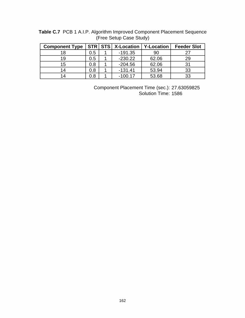
Table C.7 PCB 1 A.I.P. Algorithm Improved Component Placement Sequence(Free Setup Case Study)
Component Type STR STS X-Location Y-Location Feeder Slot18 0.5 1 -191.35 90 2719 0.5 1 -230.22 62.06 2915 0.8 1 -204.56 62.06 3114 0.8 1 -131.41 53.94 3314 0.8 1 -100.17 53.68 33
27.630598251586Solution Time:
Component Placement Time (sec.):
162

Table C.8 PCB 1 A.I.P. Algorithm Improved Feeder Assignment(Free Setup Case Study)
Component Type Feeder Slot STR STS Feeder Size1 20 1 0 82 19 1 0 83 15 1 0 84 17 1 0 125 21 1 0 86 12 1 0 87 13 1 0 88 14 1 0 89 10 0.8 0 12
10 8 0.6 0 1211 6 0.5 0 1612 4 0.5 0 1613 2 0.5 0 1614 33 0.8 1 1215 31 0.8 1 1216 23 0.5 1 1617 25 0.5 1 1618 27 0.5 1 1619 29 0.5 1 16
163

Table C.9 PCB 1 N.N. Algorithm Initial Placement Sequence(Free Setup Case Study)
Component Type STR STS X-Location Y-Location Feeder Slot13 0.5 0 -108.04 167.73 212 0.5 0 -190.85 101.18 411 0.5 0 -215.74 62.06 69 0.8 0 -147.92 46.57 109 0.8 0 -144.11 46.57 109 0.8 0 -140.3 46.57 109 0.8 0 -136.24 46.57 109 0.8 0 -132.17 46.57 109 0.8 0 -128.11 46.57 109 0.8 0 -124.3 46.57 109 0.8 0 -120.23 46.57 109 0.8 0 -116.42 46.57 109 0.8 0 -112.36 46.57 109 0.8 0 -108.55 46.57 109 0.8 0 -104.49 46.57 109 0.8 0 -100.42 46.57 109 0.8 0 -96.36 46.57 109 0.8 0 -92.29 46.57 109 0.8 0 -88.23 46.57 107 1 0 -155.79 51.14 138 1 0 -169.76 30.31 143 1 0 -150.71 22.69 153 1 0 -149.19 22.69 153 1 0 -123.03 22.69 153 1 0 -121.5 22.69 153 1 0 -102.2 22.69 153 1 0 -100.68 22.69 153 1 0 -89.5 22.69 153 1 0 -87.98 22.69 154 1 0 -138.52 81.88 174 1 0 -134.97 81.88 174 1 0 -142.08 81.88 174 1 0 -145.63 81.88 174 1 0 -115.66 81.88 174 1 0 -111.6 81.88 174 1 0 -107.53 81.88 174 1 0 -103.98 81.88 174 1 0 -144.36 27.77 172 1 0 -130.9 80.1 192 1 0 -121 79.34 192 1 0 -99.91 80.35 19
164

Table C.9 PCB 1 N.N. Algorithm Initial Placement Sequence(Free Setup Case Study)
Component Type STR STS X-Location Y-Location Feeder Slot2 1 0 -88.99 79.84 192 1 0 -74.01 47.84 191 1 0 -111.6 86.96 201 1 0 -142.08 86.96 201 1 0 -153.25 99.66 201 1 0 -155.79 69.68 201 1 0 -155.79 46.32 201 1 0 -183.73 59.52 201 1 0 -191.35 61.05 201 1 0 -193.89 61.05 201 1 0 -193.39 71.72 201 1 0 -191.86 71.72 201 1 0 -189.32 71.72 201 1 0 -187.8 71.72 201 1 0 -184.75 79.08 201 1 0 -187.29 82.89 201 1 0 -189.83 84.92 201 1 0 -192.88 82.89 201 1 0 -200.5 76.29 201 1 0 -195.93 71.72 201 1 0 -209.13 62.06 201 1 0 -209.64 64.1 201 1 0 -240.63 81.37 201 1 0 -243.17 90.77 201 1 0 -245.2 105.24 201 1 0 -257.9 86.45 201 1 0 -257.9 84.42 201 1 0 -257.9 82.38 201 1 0 -256.89 51.4 201 1 0 -249.77 32.6 201 1 0 -255.11 32.6 201 1 0 -258.41 32.09 201 1 0 -261.46 29.04 201 1 0 -262.98 29.04 201 1 0 -264.51 29.04 201 1 0 -266.03 29.04 201 1 0 -268.06 29.04 201 1 0 -269.59 29.04 201 1 0 -271.11 29.04 201 1 0 -272.63 29.04 201 1 0 -192.37 95.59 20
165

Table C.9 PCB 1 N.N. Algorithm Initial Placement Sequence(Free Setup Case Study)
Component Type STR STS X-Location Y-Location Feeder Slot1 1 0 -188.81 95.59 201 1 0 -195.16 141.82 201 1 0 -202.53 170.78 201 1 0 -213.45 171.03 201 1 0 -226.91 171.28 201 1 0 -239.11 171.28 201 1 0 -246.73 165.95 201 1 0 -249.52 172.05 201 1 0 -262.22 163.16 201 1 0 -239.61 125.56 202 1 0 -237.58 159.09 192 1 0 -231.49 159.6 192 1 0 -224.88 159.6 192 1 0 -229.96 170.27 192 1 0 -223.87 170.27 192 1 0 -236.57 170.27 192 1 0 -242.66 170.27 192 1 0 -243.68 159.09 195 1 0 -205.58 170.78 215 1 0 -204.05 170.78 215 1 0 -201.01 170.78 215 1 0 -199.48 170.78 215 1 0 -195.67 170.78 215 1 0 -202.28 158.84 215 1 0 -204.31 158.84 215 1 0 -205.83 158.84 211 1 0 -79.59 35.9 201 1 0 -78.07 48.35 203 1 0 -113.63 133.95 153 1 0 -107.28 103.97 153 1 0 -193.39 138.26 156 1 0 -226.91 31.33 126 1 0 -226.91 28.28 126 1 0 -226.91 23.71 126 1 0 -226.91 21.17 12
10 0.6 0 -267.55 171.28 810 0.6 0 -68.67 150.71 816 0.5 1 -95.34 167.73 2316 0.5 1 -79.09 167.73 2317 0.5 1 -191.35 111.34 2517 0.5 1 -191.35 121.5 25
166

Table C.9 PCB 1 N.N. Algorithm Initial Placement Sequence(Free Setup Case Study)
Component Type STR STS X-Location Y-Location Feeder Slot18 0.5 1 -191.35 90 2719 0.5 1 -230.22 62.06 2915 0.8 1 -204.56 62.06 3314 0.8 1 -131.41 53.94 3114 0.8 1 -100.17 53.68 31
28.793329491Solution Time:
Component Placement Time (sec.):
167

Table C.10 PCB 1 N.N. Algorithm Initial Feeder Assignment(Free Setup Case Study)
Component Type Feeder Slot STR STS Feeder Size1 20 1 0 82 19 1 0 83 15 1 0 84 17 1 0 125 21 1 0 86 12 1 0 87 13 1 0 88 14 1 0 89 10 0.8 0 12
10 8 0.6 0 1211 6 0.5 0 1612 4 0.5 0 1613 2 0.5 0 1614 31 0.8 1 1215 33 0.8 1 1216 23 0.5 1 1617 25 0.5 1 1618 27 0.5 1 1619 29 0.5 1 16
168

Table C.11 PCB 1 N.N. Algorithm Improved Component Placement Sequence(Free Setup Case Study)
Component Type STR STS X-Location Y-Location Feeder Slot13 0.5 0 -108.04 167.73 211 0.5 0 -215.74 62.06 612 0.5 0 -190.85 101.18 47 1 0 -155.79 51.14 139 0.8 0 -116.42 46.57 89 0.8 0 -108.55 46.57 89 0.8 0 -100.42 46.57 89 0.8 0 -92.29 46.57 89 0.8 0 -88.23 46.57 89 0.8 0 -96.36 46.57 89 0.8 0 -104.49 46.57 89 0.8 0 -112.36 46.57 89 0.8 0 -120.23 46.57 89 0.8 0 -124.3 46.57 89 0.8 0 -128.11 46.57 89 0.8 0 -132.17 46.57 89 0.8 0 -136.24 46.57 89 0.8 0 -140.3 46.57 89 0.8 0 -144.11 46.57 89 0.8 0 -147.92 46.57 86 1 0 -226.91 31.33 126 1 0 -226.91 28.28 126 1 0 -226.91 23.71 128 1 0 -169.76 30.31 143 1 0 -150.71 22.69 153 1 0 -149.19 22.69 153 1 0 -87.98 22.69 153 1 0 -89.5 22.69 153 1 0 -100.68 22.69 153 1 0 -102.2 22.69 153 1 0 -121.5 22.69 153 1 0 -123.03 22.69 154 1 0 -144.36 27.77 174 1 0 -138.52 81.88 174 1 0 -142.08 81.88 174 1 0 -145.63 81.88 174 1 0 -134.97 81.88 174 1 0 -103.98 81.88 174 1 0 -107.53 81.88 174 1 0 -111.6 81.88 174 1 0 -115.66 81.88 17
169

Table C.11 PCB 1 N.N. Algorithm Improved Component Placement Sequence(Free Setup Case Study)
Component Type STR STS X-Location Y-Location Feeder Slot2 1 0 -121 79.34 192 1 0 -130.9 80.1 191 1 0 -155.79 69.68 201 1 0 -155.79 46.32 201 1 0 -183.73 59.52 201 1 0 -191.35 61.05 201 1 0 -193.89 61.05 201 1 0 -193.39 71.72 201 1 0 -192.88 82.89 201 1 0 -192.37 95.59 201 1 0 -188.81 95.59 201 1 0 -187.29 82.89 201 1 0 -187.8 71.72 201 1 0 -184.75 79.08 201 1 0 -189.32 71.72 201 1 0 -191.86 71.72 201 1 0 -189.83 84.92 201 1 0 -195.93 71.72 201 1 0 -209.13 62.06 201 1 0 -200.5 76.29 201 1 0 -209.64 64.1 201 1 0 -249.77 32.6 201 1 0 -258.41 32.09 201 1 0 -262.98 29.04 201 1 0 -266.03 29.04 201 1 0 -269.59 29.04 201 1 0 -272.63 29.04 201 1 0 -271.11 29.04 201 1 0 -268.06 29.04 201 1 0 -264.51 29.04 201 1 0 -261.46 29.04 201 1 0 -255.11 32.6 201 1 0 -256.89 51.4 201 1 0 -240.63 81.37 201 1 0 -257.9 86.45 201 1 0 -257.9 84.42 201 1 0 -257.9 82.38 201 1 0 -243.17 90.77 201 1 0 -245.2 105.24 201 1 0 -239.61 125.56 201 1 0 -262.22 163.16 20
170

Table C.11 PCB 1 N.N. Algorithm Improved Component Placement Sequence(Free Setup Case Study)
Component Type STR STS X-Location Y-Location Feeder Slot1 1 0 -249.52 172.05 201 1 0 -246.73 165.95 201 1 0 -239.11 171.28 201 1 0 -226.91 171.28 201 1 0 -213.45 171.03 202 1 0 -224.88 159.6 192 1 0 -236.57 170.27 192 1 0 -243.68 159.09 192 1 0 -242.66 170.27 192 1 0 -229.96 170.27 192 1 0 -231.49 159.6 192 1 0 -237.58 159.09 192 1 0 -223.87 170.27 195 1 0 -205.83 158.84 215 1 0 -204.31 158.84 215 1 0 -202.28 158.84 215 1 0 -195.67 170.78 215 1 0 -199.48 170.78 215 1 0 -201.01 170.78 215 1 0 -204.05 170.78 215 1 0 -205.58 170.78 211 1 0 -202.53 170.78 201 1 0 -195.16 141.82 201 1 0 -153.25 99.66 201 1 0 -142.08 86.96 201 1 0 -111.6 86.96 201 1 0 -78.07 48.35 201 1 0 -79.59 35.9 202 1 0 -74.01 47.84 192 1 0 -88.99 79.84 192 1 0 -99.91 80.35 193 1 0 -193.39 138.26 153 1 0 -107.28 103.97 153 1 0 -113.63 133.95 156 1 0 -226.91 21.17 12
10 0.6 0 -267.55 171.28 1010 0.6 0 -68.67 150.71 1016 0.5 1 -79.09 167.73 2316 0.5 1 -95.34 167.73 2317 0.5 1 -191.35 111.34 2517 0.5 1 -191.35 121.5 25
171

Table C.11 PCB 1 N.N. Algorithm Improved Component Placement Sequence(Free Setup Case Study)
Component Type STR STS X-Location Y-Location Feeder Slot18 0.5 1 -191.35 90 2719 0.5 1 -230.22 62.06 2915 0.8 1 -204.56 62.06 3114 0.8 1 -131.41 53.94 3314 0.8 1 -100.17 53.68 33
28.135912463322Solution Time:
Component Placement Time (sec.):
172
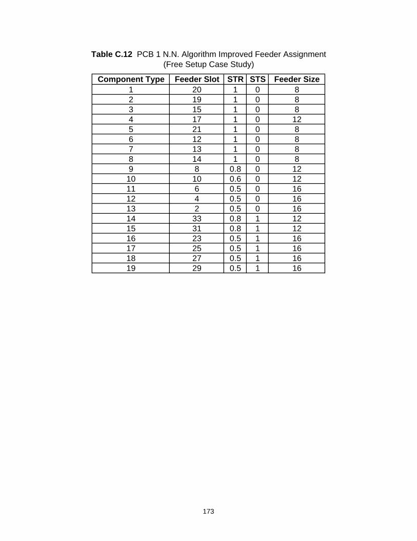
Table C.12 PCB 1 N.N. Algorithm Improved Feeder Assignment(Free Setup Case Study)
Component Type Feeder Slot STR STS Feeder Size1 20 1 0 82 19 1 0 83 15 1 0 84 17 1 0 125 21 1 0 86 12 1 0 87 13 1 0 88 14 1 0 89 8 0.8 0 12
10 10 0.6 0 1211 6 0.5 0 1612 4 0.5 0 1613 2 0.5 0 1614 33 0.8 1 1215 31 0.8 1 1216 23 0.5 1 1617 25 0.5 1 1618 27 0.5 1 1619 29 0.5 1 16
173

Table C.13 PCB 5 Component Type Data(Fixed Setup Case Study)
Type Number STR STS Feeder Size Feeder Status1 1 0 8 1 Fixed2 1 0 8 3 Fixed3 1 0 8 5 Fixed4 1 0 8 7 Fixed5 1 0 8 10 Fixed6 1 0 8 12 Fixed7 1 0 8 17 Fixed8 1 0 8 22 Fixed9 1 0 8 30 Fixed
10 1 0 8 40 Fixed11 1 0 8 43 Fixed12 1 0 8 45 Fixed13 1 0 8 46 Fixed14 0.6 0 12 57 Fixed15 1 0 8 61 Fixed16 1 0 8 63 Fixed17 1 0 8 74 Fixed18 1 0 8 78 Fixed19 1 0 8 79 Fixed20 1 0 8 85 Fixed21 0.9 0 8 87 Fixed
The Status column indicates whether a component type has a pre-assigned feeder slot location. If the component type has a pre-assigned feeder slot location, the Status column indicates "Fixed" and the Feeder column indicates the feeder slot location to which the component type has been pre-assigned. If the component type does not have a pre-assigned feeder slot location, the Status column and the Feeder column are empty. This indicates that the feeder assignment for that specific component type has to be determined. The rows in which the text is Bold and Italized indicate that the component type listed in that row is not used in the PCB being addressed. This component type, however, occupies the feeder slot location indicated in the Feeder column. Note that all component types with pre-assigned feeder slot locations cannot be reassigned to any other feeder slot locations. In addition, the feeder slot locations associated with these component types can not be re-assigned to any other component types.
174
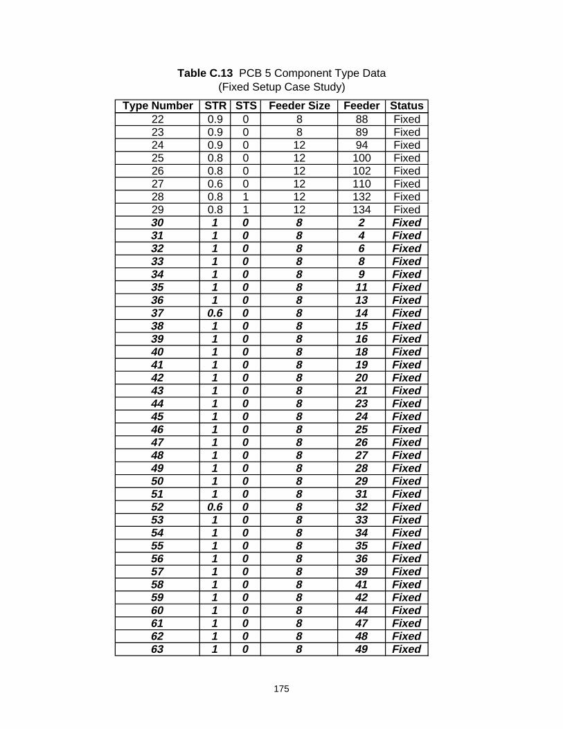
Table C.13 PCB 5 Component Type Data(Fixed Setup Case Study)
Type Number STR STS Feeder Size Feeder Status22 0.9 0 8 88 Fixed23 0.9 0 8 89 Fixed24 0.9 0 12 94 Fixed25 0.8 0 12 100 Fixed26 0.8 0 12 102 Fixed27 0.6 0 12 110 Fixed28 0.8 1 12 132 Fixed29 0.8 1 12 134 Fixed30 1 0 8 2 Fixed31 1 0 8 4 Fixed32 1 0 8 6 Fixed33 1 0 8 8 Fixed34 1 0 8 9 Fixed35 1 0 8 11 Fixed36 1 0 8 13 Fixed37 0.6 0 8 14 Fixed38 1 0 8 15 Fixed39 1 0 8 16 Fixed40 1 0 8 18 Fixed41 1 0 8 19 Fixed42 1 0 8 20 Fixed43 1 0 8 21 Fixed44 1 0 8 23 Fixed45 1 0 8 24 Fixed46 1 0 8 25 Fixed47 1 0 8 26 Fixed48 1 0 8 27 Fixed49 1 0 8 28 Fixed50 1 0 8 29 Fixed51 1 0 8 31 Fixed52 0.6 0 8 32 Fixed53 1 0 8 33 Fixed54 1 0 8 34 Fixed55 1 0 8 35 Fixed56 1 0 8 36 Fixed57 1 0 8 39 Fixed58 1 0 8 41 Fixed59 1 0 8 42 Fixed60 1 0 8 44 Fixed61 1 0 8 47 Fixed62 1 0 8 48 Fixed63 1 0 8 49 Fixed
175

Table C.13 PCB 5 Component Type Data(Fixed Setup Case Study)
Type Number STR STS Feeder Size Feeder Status64 1 0 8 50 Fixed65 1 0 8 51 Fixed66 1 0 8 52 Fixed67 1 0 8 53 Fixed68 1 0 8 54 Fixed69 1 0 8 55 Fixed70 0.6 0 12 59 Fixed71 1 0 8 62 Fixed72 1 0 8 64 Fixed73 1 0 8 65 Fixed74 1 0 8 66 Fixed75 1 0 8 67 Fixed76 1 0 8 68 Fixed77 1 0 8 69 Fixed78 1 0 8 70 Fixed79 1 0 8 71 Fixed80 1 0 8 72 Fixed81 1 0 8 73 Fixed82 1 0 8 75 Fixed83 1 0 8 76 Fixed84 1 0 8 77 Fixed85 1 0 8 80 Fixed86 1 0 8 81 Fixed87 1 0 8 82 Fixed88 1 0 8 83 Fixed89 1 0 8 84 Fixed90 1 0 8 86 Fixed91 0.9 0 8 90 Fixed92 0.8 0 12 92 Fixed93 0.8 0 12 96 Fixed94 0.8 0 12 98 Fixed95 0.8 0 12 104 Fixed96 0.6 0 12 106 Fixed97 0.6 0 12 108 Fixed98 0.6 0 16 112 Fixed99 0.6 0 16 114 Fixed100 0.5 0 16 116 Fixed101 0.6 0 16 118 Fixed102 0.8 1 8 120 Fixed103 0.8 1 12 122 Fixed104 0.8 1 12 124 Fixed105 0.8 1 12 126 Fixed
176

Table C.13 PCB 5 Component Type Data(Fixed Setup Case Study)
Type Number STR STS Feeder Size Feeder Status106 0.8 1 12 128 Fixed107 0.8 1 12 130 Fixed108 0.8 1 12 136 Fixed109 0.6 0 16 138 Fixed110 0.5 1 16 140 Fixed111 0.5 1 16 142 Fixed112 0.5 1 16 144 Fixed113 0.6 0 16 146 Fixed114 0.6 0 12 148 Fixed115 0.5 1 16 150 Fixed116 0.5 1 16 152 Fixed117 0.5 1 16 154 Fixed118 0.5 1 16 156 Fixed
177
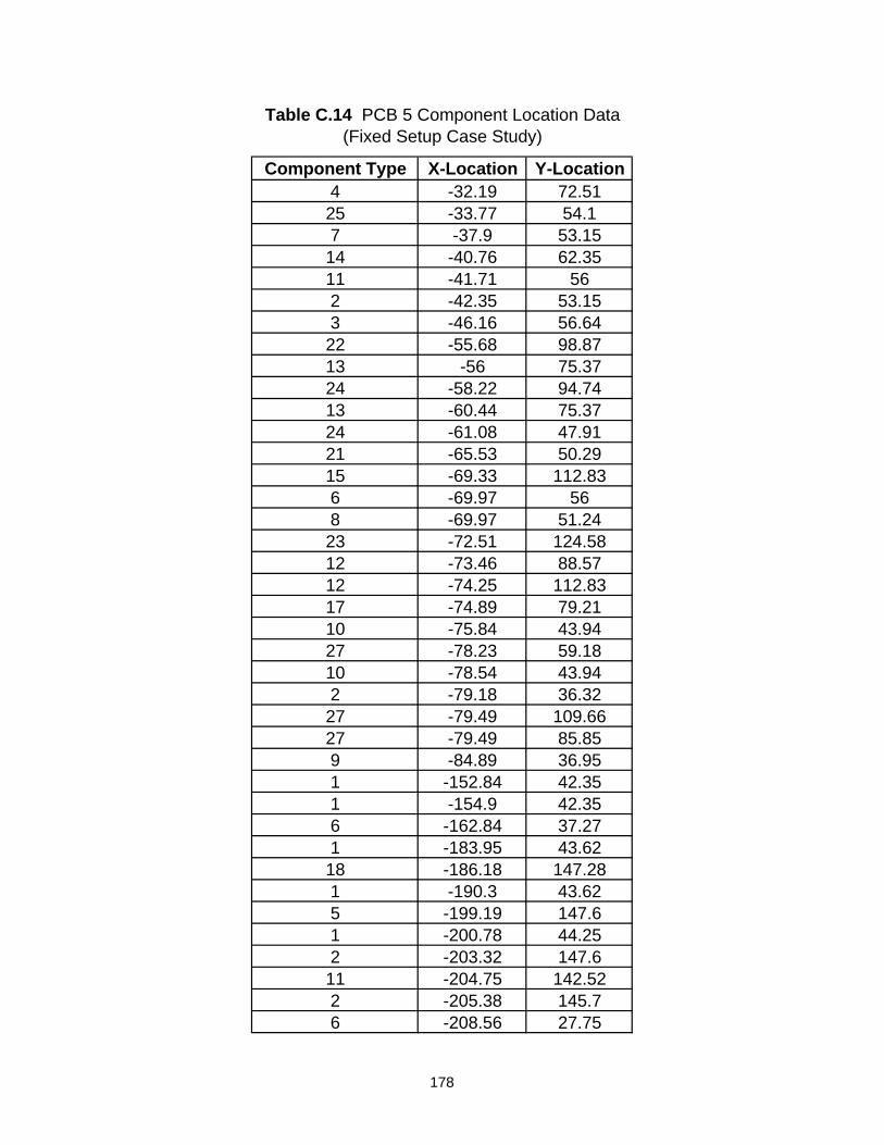
Table C.14 PCB 5 Component Location Data(Fixed Setup Case Study)
Component Type X-Location Y-Location4 -32.19 72.5125 -33.77 54.17 -37.9 53.1514 -40.76 62.3511 -41.71 562 -42.35 53.153 -46.16 56.6422 -55.68 98.8713 -56 75.3724 -58.22 94.7413 -60.44 75.3724 -61.08 47.9121 -65.53 50.2915 -69.33 112.836 -69.97 568 -69.97 51.2423 -72.51 124.5812 -73.46 88.5712 -74.25 112.8317 -74.89 79.2110 -75.84 43.9427 -78.23 59.1810 -78.54 43.942 -79.18 36.3227 -79.49 109.6627 -79.49 85.859 -84.89 36.951 -152.84 42.351 -154.9 42.356 -162.84 37.271 -183.95 43.6218 -186.18 147.281 -190.3 43.625 -199.19 147.61 -200.78 44.252 -203.32 147.611 -204.75 142.522 -205.38 145.76 -208.56 27.75
178

Table C.14 PCB 5 Component Location Data(Fixed Setup Case Study)
Component Type X-Location Y-Location29 -210.31 145.728 -213.48 30.619 -219.04 144.7416 -220.94 141.7326 -223.96 147.1220 -226.18 112.419 -238.08 59.182 -239.2 65.531 -239.67 52.99
179

Table C.15 PCB 5 Commercial Software Component Placement Sequence(Fixed Setup Case Study)
Component Type STR STS X-Location Y-Location Feeder Slot2 1 0 -42.35 53.15 32 1 0 -79.18 36.32 32 1 0 -239.2 65.53 32 1 0 -205.38 145.7 32 1 0 -203.32 147.6 31 1 0 -239.67 52.99 11 1 0 -200.78 44.25 11 1 0 -190.3 43.62 11 1 0 -183.95 43.62 11 1 0 -154.9 42.35 11 1 0 -152.84 42.35 13 1 0 -46.16 56.64 54 1 0 -32.19 72.51 76 1 0 -69.97 56 126 1 0 -162.84 37.27 126 1 0 -208.56 27.75 125 1 0 -199.19 147.6 107 1 0 -37.9 53.15 178 1 0 -69.97 51.24 229 1 0 -84.89 36.95 309 1 0 -238.08 59.18 3010 1 0 -78.54 43.94 4010 1 0 -75.84 43.94 4011 1 0 -41.71 56 4312 1 0 -73.46 88.57 4512 1 0 -74.25 112.83 4511 1 0 -204.75 142.52 4313 1 0 -60.44 75.37 4613 1 0 -56 75.37 4614 0.6 0 -40.76 62.35 5715 1 0 -69.33 112.83 6116 1 0 -220.94 141.73 6317 1 0 -74.89 79.21 7418 1 0 -186.18 147.28 7819 1 0 -219.04 144.74 7920 1 0 -226.18 112.41 8522 0.9 0 -55.68 98.87 8823 0.9 0 -72.51 124.58 8921 0.9 0 -65.53 50.29 87
180

Table C.15 PCB 5 Commercial Software Component Placement Sequence(Fixed Setup Case Study)
Component Type STR STS X-Location Y-Location Feeder Slot24 0.9 0 -61.08 47.91 9424 0.9 0 -58.22 94.74 9425 0.8 0 -33.77 54.1 10026 0.8 0 -223.96 147.12 10227 0.6 0 -79.49 109.66 11027 0.6 0 -79.49 85.85 11027 0.6 0 -78.23 59.18 11028 0.8 1 -213.48 30.6 13229 0.8 1 -210.31 145.7 134
17.18121542Component Placement Time (sec.):
181

Table C.16 PCB 5 Commercial Software Feeder Assignment(Fixed Setup Case Study)
Component Type Feeder Slot STR STS Feeder Size1 1 1 0 82 3 1 0 83 5 1 0 84 7 1 0 85 10 1 0 86 12 1 0 87 17 1 0 88 22 1 0 89 30 1 0 810 40 1 0 811 43 1 0 812 45 1 0 813 46 1 0 814 57 0.6 0 1215 61 1 0 816 63 1 0 817 74 1 0 818 78 1 0 819 79 1 0 820 85 1 0 821 87 0.9 0 822 88 0.9 0 823 89 0.9 0 824 94 0.9 0 1225 100 0.8 0 1226 102 0.8 0 1227 110 0.6 0 1228 132 0.8 1 1229 134 0.8 1 12
182

Table C.17 PCB 5 A.I.P. Algorithm Initial Component Placement Sequence(Fixed Setup Case Study)
Component Type STR STS X-Location Y-Location Feeder Slot1 1 0 -239.67 52.99 11 1 0 -200.78 44.25 11 1 0 -190.3 43.62 11 1 0 -183.95 43.62 11 1 0 -152.84 42.35 11 1 0 -154.9 42.35 12 1 0 -239.2 65.53 32 1 0 -205.38 145.7 32 1 0 -203.32 147.6 32 1 0 -79.18 36.32 32 1 0 -42.35 53.15 33 1 0 -46.16 56.64 54 1 0 -32.19 72.51 75 1 0 -199.19 147.6 106 1 0 -69.97 56 126 1 0 -162.84 37.27 126 1 0 -208.56 27.75 127 1 0 -37.9 53.15 178 1 0 -69.97 51.24 229 1 0 -84.89 36.95 309 1 0 -238.08 59.18 3010 1 0 -75.84 43.94 4010 1 0 -78.54 43.94 4011 1 0 -204.75 142.52 4311 1 0 -41.71 56 4312 1 0 -74.25 112.83 4512 1 0 -73.46 88.57 4513 1 0 -56 75.37 4613 1 0 -60.44 75.37 4614 0.6 0 -40.76 62.35 5715 1 0 -69.33 112.83 6116 1 0 -220.94 141.73 6317 1 0 -74.89 79.21 7418 1 0 -186.18 147.28 7819 1 0 -219.04 144.74 7920 1 0 -226.18 112.41 8521 0.9 0 -65.53 50.29 8722 0.9 0 -55.68 98.87 8823 0.9 0 -72.51 124.58 8924 0.9 0 -58.22 94.74 9424 0.9 0 -61.08 47.91 9425 0.8 0 -33.77 54.1 10026 0.8 0 -223.96 147.12 10227 0.6 0 -79.49 109.66 110
183

Table C.17 PCB 5 A.I.P. Algorithm Initial Component Placement Sequence(Fixed Setup Case Study)
Component Type STR STS X-Location Y-Location Feeder Slot29 0.8 1 -210.31 145.7 13428 0.8 1 -213.48 30.6 13227 0.6 0 -78.23 59.18 11027 0.6 0 -79.49 85.85 110
17.549520960Solution Time:
Component Placement Time (sec.):
184

Table C.18 PCB 5 A.I.P. Algorithm Initial Feeder Assignment(Fixed Setup Case Study)
Component Type Feeder Slot STR STS Feeder Size1 1 1 0 82 3 1 0 83 5 1 0 84 7 1 0 85 10 1 0 86 12 1 0 87 17 1 0 88 22 1 0 89 30 1 0 810 40 1 0 811 43 1 0 812 45 1 0 813 46 1 0 814 57 0.6 0 1215 61 1 0 816 63 1 0 817 74 1 0 818 78 1 0 819 79 1 0 820 85 1 0 821 87 0.9 0 822 88 0.9 0 823 89 0.9 0 824 94 0.9 0 1225 100 0.8 0 1226 102 0.8 0 1227 110 0.6 0 1228 132 0.8 1 1229 134 0.8 1 12
185
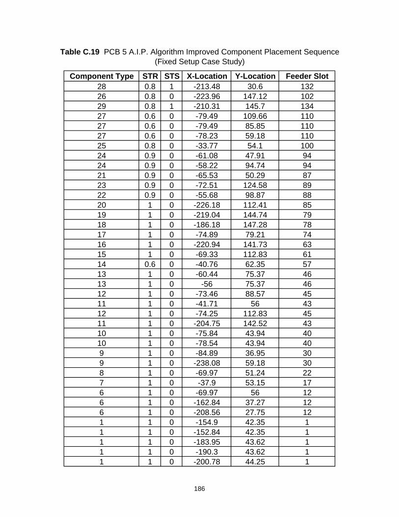
Table C.19 PCB 5 A.I.P. Algorithm Improved Component Placement Sequence(Fixed Setup Case Study)
Component Type STR STS X-Location Y-Location Feeder Slot28 0.8 1 -213.48 30.6 13226 0.8 0 -223.96 147.12 10229 0.8 1 -210.31 145.7 13427 0.6 0 -79.49 109.66 11027 0.6 0 -79.49 85.85 11027 0.6 0 -78.23 59.18 11025 0.8 0 -33.77 54.1 10024 0.9 0 -61.08 47.91 9424 0.9 0 -58.22 94.74 9421 0.9 0 -65.53 50.29 8723 0.9 0 -72.51 124.58 8922 0.9 0 -55.68 98.87 8820 1 0 -226.18 112.41 8519 1 0 -219.04 144.74 7918 1 0 -186.18 147.28 7817 1 0 -74.89 79.21 7416 1 0 -220.94 141.73 6315 1 0 -69.33 112.83 6114 0.6 0 -40.76 62.35 5713 1 0 -60.44 75.37 4613 1 0 -56 75.37 4612 1 0 -73.46 88.57 4511 1 0 -41.71 56 4312 1 0 -74.25 112.83 4511 1 0 -204.75 142.52 4310 1 0 -75.84 43.94 4010 1 0 -78.54 43.94 409 1 0 -84.89 36.95 309 1 0 -238.08 59.18 308 1 0 -69.97 51.24 227 1 0 -37.9 53.15 176 1 0 -69.97 56 126 1 0 -162.84 37.27 126 1 0 -208.56 27.75 121 1 0 -154.9 42.35 11 1 0 -152.84 42.35 11 1 0 -183.95 43.62 11 1 0 -190.3 43.62 11 1 0 -200.78 44.25 1
186
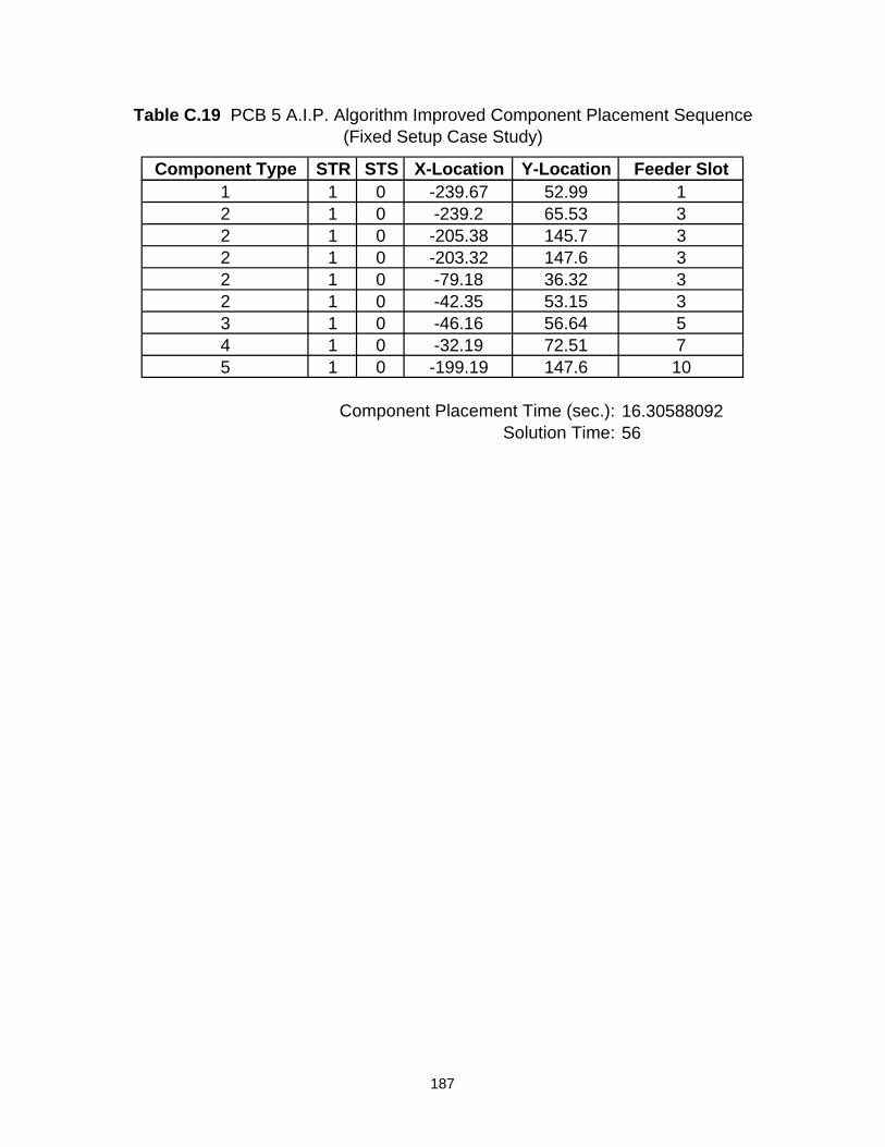
Table C.19 PCB 5 A.I.P. Algorithm Improved Component Placement Sequence(Fixed Setup Case Study)
Component Type STR STS X-Location Y-Location Feeder Slot1 1 0 -239.67 52.99 12 1 0 -239.2 65.53 32 1 0 -205.38 145.7 32 1 0 -203.32 147.6 32 1 0 -79.18 36.32 32 1 0 -42.35 53.15 33 1 0 -46.16 56.64 54 1 0 -32.19 72.51 75 1 0 -199.19 147.6 10
16.3058809256Solution Time:
Component Placement Time (sec.):
187
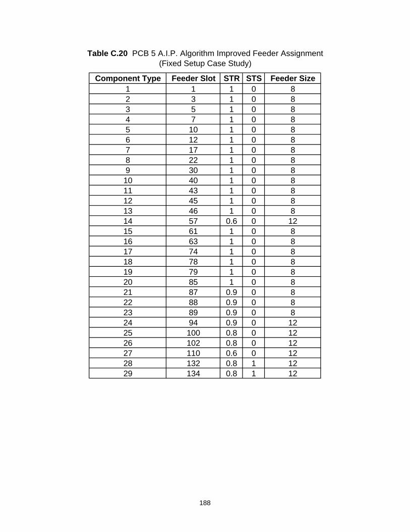
Table C.20 PCB 5 A.I.P. Algorithm Improved Feeder Assignment(Fixed Setup Case Study)
Component Type Feeder Slot STR STS Feeder Size1 1 1 0 82 3 1 0 83 5 1 0 84 7 1 0 85 10 1 0 86 12 1 0 87 17 1 0 88 22 1 0 89 30 1 0 810 40 1 0 811 43 1 0 812 45 1 0 813 46 1 0 814 57 0.6 0 1215 61 1 0 816 63 1 0 817 74 1 0 818 78 1 0 819 79 1 0 820 85 1 0 821 87 0.9 0 822 88 0.9 0 823 89 0.9 0 824 94 0.9 0 1225 100 0.8 0 1226 102 0.8 0 1227 110 0.6 0 1228 132 0.8 1 1229 134 0.8 1 12
188

Table C.21 PCB 5 N.N. Algorithm Initial Component Placement Sequence(Fixed Setup Case Study)
Component Type STR STS X-Location Y-Location Feeder Slot1 1 0 -239.67 52.99 11 1 0 -200.78 44.25 11 1 0 -190.3 43.62 11 1 0 -183.95 43.62 11 1 0 -154.9 42.35 11 1 0 -152.84 42.35 12 1 0 -79.18 36.32 32 1 0 -42.35 53.15 33 1 0 -46.16 56.64 54 1 0 -32.19 72.51 76 1 0 -69.97 56 126 1 0 -162.84 37.27 126 1 0 -208.56 27.75 125 1 0 -199.19 147.6 107 1 0 -37.9 53.15 178 1 0 -69.97 51.24 229 1 0 -84.89 36.95 309 1 0 -238.08 59.18 3010 1 0 -75.84 43.94 4010 1 0 -78.54 43.94 4011 1 0 -41.71 56 4312 1 0 -73.46 88.57 4512 1 0 -74.25 112.83 4513 1 0 -60.44 75.37 4613 1 0 -56 75.37 4611 1 0 -204.75 142.52 4314 0.6 0 -40.76 62.35 5716 1 0 -220.94 141.73 6315 1 0 -69.33 112.83 6117 1 0 -74.89 79.21 7418 1 0 -186.18 147.28 7819 1 0 -219.04 144.74 7920 1 0 -226.18 112.41 8523 0.9 0 -72.51 124.58 8922 0.9 0 -55.68 98.87 8821 0.9 0 -65.53 50.29 8724 0.9 0 -58.22 94.74 9424 0.9 0 -61.08 47.91 9425 0.8 0 -33.77 54.1 100
189

Table C.21 PCB 5 N.N. Algorithm Initial Component Placement Sequence(Fixed Setup Case Study)
Component Type STR STS X-Location Y-Location Feeder Slot26 0.8 0 -223.96 147.12 10227 0.6 0 -79.49 85.85 11027 0.6 0 -79.49 109.66 11027 0.6 0 -78.23 59.18 1102 1 0 -239.2 65.53 32 1 0 -205.38 145.7 32 1 0 -203.32 147.6 328 0.8 1 -213.48 30.6 13229 0.8 1 -210.31 145.7 134
23.238110950Solution Time:
Component Placement Time (sec.):
190

Table C.22 PCB 5 N.N. Algorithm Initial Feeder Assignment(Fixed Setup Case Study)
Component Type Feeder Slot STR STS Feeder Size1 1 1 0 82 3 1 0 83 5 1 0 84 7 1 0 85 10 1 0 86 12 1 0 87 17 1 0 88 22 1 0 89 30 1 0 810 40 1 0 811 43 1 0 812 45 1 0 813 46 1 0 814 57 0.6 0 1215 61 1 0 816 63 1 0 817 74 1 0 818 78 1 0 819 79 1 0 820 85 1 0 821 87 0.9 0 822 88 0.9 0 823 89 0.9 0 824 94 0.9 0 1225 100 0.8 0 1226 102 0.8 0 1227 110 0.6 0 1228 132 0.8 1 1229 134 0.8 1 12
191

Table C.23 PCB 5 N.N. Algorithm Improved Component Placement Sequence(Fixed Setup Case Study)
Component Type STR STS X-Location Y-Location Feeder Slot4 1 0 -32.19 72.51 73 1 0 -46.16 56.64 52 1 0 -42.35 53.15 32 1 0 -79.18 36.32 36 1 0 -162.84 37.27 126 1 0 -208.56 27.75 121 1 0 -152.84 42.35 11 1 0 -154.9 42.35 11 1 0 -183.95 43.62 11 1 0 -239.67 52.99 11 1 0 -200.78 44.25 11 1 0 -190.3 43.62 12 1 0 -239.2 65.53 32 1 0 -205.38 145.7 32 1 0 -203.32 147.6 35 1 0 -199.19 147.6 106 1 0 -69.97 56 127 1 0 -37.9 53.15 178 1 0 -69.97 51.24 229 1 0 -84.89 36.95 309 1 0 -238.08 59.18 3010 1 0 -78.54 43.94 4010 1 0 -75.84 43.94 4011 1 0 -204.75 142.52 4312 1 0 -74.25 112.83 4512 1 0 -73.46 88.57 4511 1 0 -41.71 56 4313 1 0 -60.44 75.37 4613 1 0 -56 75.37 4614 0.6 0 -40.76 62.35 5715 1 0 -69.33 112.83 6116 1 0 -220.94 141.73 6317 1 0 -74.89 79.21 7418 1 0 -186.18 147.28 7819 1 0 -219.04 144.74 7920 1 0 -226.18 112.41 8521 0.9 0 -65.53 50.29 8722 0.9 0 -55.68 98.87 8823 0.9 0 -72.51 124.58 89
192

Table C.23 PCB 5 N.N. Algorithm Improved Component Placement Sequence(Fixed Setup Case Study)
Component Type STR STS X-Location Y-Location Feeder Slot24 0.9 0 -58.22 94.74 9424 0.9 0 -61.08 47.91 9425 0.8 0 -33.77 54.1 10026 0.8 0 -223.96 147.12 10227 0.6 0 -79.49 109.66 11027 0.6 0 -78.23 59.18 11027 0.6 0 -79.49 85.85 11028 0.8 1 -213.48 30.6 13229 0.8 1 -210.31 145.7 134
16.42652229126Solution Time:
Component Placement Time (sec.):
193

Table C.24 PCB 5 N.N. Algorithm Improved Feeder Assignment(Fixed Setup Case Study)
Component Type Feeder Slot STR STS Feeder Size1 1 1 0 82 3 1 0 83 5 1 0 84 7 1 0 85 10 1 0 86 12 1 0 87 17 1 0 88 22 1 0 89 30 1 0 810 40 1 0 811 43 1 0 812 45 1 0 813 46 1 0 814 57 0.6 0 1215 61 1 0 816 63 1 0 817 74 1 0 818 78 1 0 819 79 1 0 820 85 1 0 821 87 0.9 0 822 88 0.9 0 823 89 0.9 0 824 94 0.9 0 1225 100 0.8 0 1226 102 0.8 0 1227 110 0.6 0 1228 132 0.8 1 1229 134 0.8 1 12
194

Table C.25 PCB 13 Component Type Data(Partial Fixed Setup Case Study)
Type Number STR STS Feeder Size Feeder Status1 1 0 8 3 Fixed2 1 0 8 9 Fixed3 1 0 8 29 Fixed4 1 0 8 37 Fixed5 1 0 8 40 Fixed6 1 0 8 44 Fixed7 1 0 8 48 Fixed8 1 0 8 66 Fixed9 1 0 8 83 Fixed
10 1 0 811 1 0 812 1 0 813 1 0 814 1 0 815 1 0 816 0.8 0 817 N/A N/A 8 7 Fixed18 N/A N/A 8 13 Fixed19 N/A N/A 8 27 Fixed20 N/A N/A 8 31 Fixed21 N/A N/A 8 43 Fixed22 N/A N/A 8 45 Fixed
The Status column indicates whether a component type has a pre-assigned feeder slot location. If the component type has a pre-assigned feeder slot location, the Status column indicates "Fixed" and the Feeder column indicates the feeder slot location to which the component type has been pre-assigned. If the component type does not have a pre-assigned feeder slot location, the Status column and the Feeder column are empty. This indicates that the feeder assignment for that specific component type has to be determined. The rows in which the text is Bold and Italized indicate that the component type listed in that row is not used in the PCB being addressed. This component type, however, occupies the feeder slot location indicated in the Feeder column. Note that all component types with pre-assigned feeder slot locations cannot be reassigned to any other feeder slot locations. In addition, the feeder slot locations associated with these component types can not be re-assigned to any other component types.
195

Table C.25 PCB 13 Component Type Data(Partial Fixed Setup Case Study)
Type Number STR STS Feeder Size Feeder Status23 N/A N/A 8 49 Fixed24 N/A N/A 8 75 Fixed25 N/A N/A 12 78 Fixed26 N/A N/A 8 82 Fixed27 N/A N/A 8 85 Fixed28 N/A N/A 12 87 Fixed29 N/A N/A 16 89 Fixed30 N/A N/A 8 91 Fixed31 N/A N/A 12 93 Fixed32 N/A N/A 8 1 Fixed33 N/A N/A 8 2 Fixed34 N/A N/A 8 4 Fixed35 N/A N/A 8 5 Fixed36 N/A N/A 8 6 Fixed37 N/A N/A 8 8 Fixed38 N/A N/A 8 10 Fixed39 N/A N/A 8 11 Fixed40 N/A N/A 8 12 Fixed41 N/A N/A 12 15 Fixed42 N/A N/A 8 17 Fixed43 N/A N/A 8 18 Fixed44 N/A N/A 8 19 Fixed45 N/A N/A 8 20 Fixed46 N/A N/A 8 21 Fixed47 N/A N/A 8 22 Fixed48 N/A N/A 8 23 Fixed49 N/A N/A 8 24 Fixed50 N/A N/A 8 25 Fixed51 N/A N/A 8 26 Fixed52 N/A N/A 8 28 Fixed53 N/A N/A 8 30 Fixed54 N/A N/A 8 32 Fixed55 N/A N/A 8 33 Fixed56 N/A N/A 8 34 Fixed57 N/A N/A 8 35 Fixed58 N/A N/A 8 36 Fixed59 N/A N/A 8 38 Fixed60 N/A N/A 8 39 Fixed61 N/A N/A 8 41 Fixed62 N/A N/A 8 42 Fixed63 N/A N/A 8 46 Fixed64 N/A N/A 8 47 Fixed
196

Table C.25 PCB 13 Component Type Data(Partial Fixed Setup Case Study)
Type Number STR STS Feeder Size Feeder Status65 N/A N/A 8 50 Fixed66 N/A N/A 8 51 Fixed67 N/A N/A 8 52 Fixed68 N/A N/A 8 53 Fixed69 N/A N/A 8 54 Fixed70 N/A N/A 8 55 Fixed71 N/A N/A 8 56 Fixed72 N/A N/A 8 57 Fixed73 N/A N/A 8 58 Fixed74 N/A N/A 8 59 Fixed75 N/A N/A 8 60 Fixed76 N/A N/A 8 61 Fixed77 N/A N/A 8 62 Fixed78 N/A N/A 8 63 Fixed79 N/A N/A 8 64 Fixed80 N/A N/A 8 65 Fixed81 N/A N/A 8 67 Fixed82 N/A N/A 8 68 Fixed83 N/A N/A 8 69 Fixed84 N/A N/A 12 71 Fixed85 N/A N/A 8 73 Fixed86 N/A N/A 8 74 Fixed87 N/A N/A 8 76 Fixed88 N/A N/A 12 80 Fixed89 N/A N/A 8 84 Fixed
197

Table C.26 PCB 13 Component Location Data(Partial Fixed Setup Case Study)
Component Type X-Location Y-Location1 -7.85 68.451 -24.96 55.121 -87.19 52.583 -118.94 102.752 -119.24 87.517 -120.21 89.417 -120.21 91.957 -120.21 94.497 -120.21 97.033 -120.84 102.753 -122.75 102.753 -124.65 102.7516 -125.59 77.043 -126.56 102.755 -128.95 87.994 -129.25 79.19 -130.37 103.3812 -135.3 93.554 -144.97 103.238 -144.97 104.659 -145.13 100.3611 -146.4 91.1614 -147.18 81.493 -149.09 95.285 -150.06 76.4110 -152.6 92.5810 -154.17 75.148 -154.35 87.3513 -156.41 75.776 -157.52 86.723 -160.06 86.249 -160.7 74.329 -160.7 77.989 -288.48 54.828 -288.79 51.3115 -292.6 54.82
198

Table C.27 PCB 13 Commercial Software Component Placement Sequence(Partial Fixed Setup)
Component Type STR STS X-Location Y-Location Feeder Slot1 1 0 -7.85 68.45 31 1 0 -24.96 55.12 31 1 0 -87.19 52.58 32 1 0 -119.24 87.51 93 1 0 -118.94 102.75 293 1 0 -120.84 102.75 293 1 0 -122.75 102.75 293 1 0 -124.65 102.75 293 1 0 -126.56 102.75 293 1 0 -149.09 95.28 293 1 0 -160.06 86.24 294 1 0 -144.97 103.23 374 1 0 -129.25 79.1 375 1 0 -128.95 87.99 405 1 0 -150.06 76.41 406 1 0 -157.52 86.72 447 1 0 -120.21 89.41 487 1 0 -120.21 91.95 487 1 0 -120.21 94.49 487 1 0 -120.21 97.03 488 1 0 -144.97 104.65 668 1 0 -154.35 87.35 668 1 0 -288.79 51.31 669 1 0 -288.48 54.82 839 1 0 -160.7 74.32 839 1 0 -160.7 77.98 839 1 0 -145.13 100.36 839 1 0 -130.37 103.38 8312 1 0 -135.3 93.55 9711 1 0 -146.4 91.16 9610 1 0 -152.6 92.58 9510 1 0 -154.17 75.14 9513 1 0 -156.41 75.77 9814 1 0 -147.18 81.49 9916 0.8 0 -125.59 77.04 10115 1 0 -292.6 54.82 100
9.895895037Component Placement Time (sec.):
199

Table C.28 PCB 13 Commercial Software Feeder Assignment(Partial Fixed Setup Case Study)
Component Type Feeder Slot STR STS Feeder Size1 3 1 0 82 9 1 0 83 29 1 0 84 37 1 0 85 40 1 0 86 44 1 0 87 48 1 0 88 66 1 0 89 83 1 0 810 95 1 0 811 96 1 0 812 97 1 0 813 98 1 0 814 99 1 0 815 100 1 0 816 101 0.8 0 8
200

Table C.29 PCB 13 A.I.P. Algorithm Initial Component Placement Sequence(Partial Fixed Setup Case Study)
Component Type STR STS X-Location Y-Location Feeder Slot1 1 0 -7.85 68.45 31 1 0 -24.96 55.12 31 1 0 -87.19 52.58 32 1 0 -119.24 87.51 93 1 0 -118.94 102.75 293 1 0 -120.84 102.75 293 1 0 -122.75 102.75 293 1 0 -124.65 102.75 293 1 0 -126.56 102.75 293 1 0 -149.09 95.28 293 1 0 -160.06 86.24 294 1 0 -129.25 79.1 374 1 0 -144.97 103.23 375 1 0 -128.95 87.99 405 1 0 -150.06 76.41 406 1 0 -157.52 86.72 447 1 0 -120.21 89.41 487 1 0 -120.21 91.95 487 1 0 -120.21 94.49 487 1 0 -120.21 97.03 488 1 0 -144.97 104.65 668 1 0 -154.35 87.35 668 1 0 -288.79 51.31 669 1 0 -130.37 103.38 839 1 0 -145.13 100.36 839 1 0 -160.7 74.32 839 1 0 -160.7 77.98 839 1 0 -288.48 54.82 8316 0.8 0 -125.59 77.04 9513 1 0 -156.41 75.77 9610 1 0 -152.6 92.58 9710 1 0 -154.17 75.14 9715 1 0 -292.6 54.82 9814 1 0 -147.18 81.49 9911 1 0 -146.4 91.16 10012 1 0 -135.3 93.55 101
10.21435950Solution Time:
Component Placement Time (sec.):
201

Table C.30 PCB 13 A.I.P. Algorithm Initial Feeder Assignment(Partial Fixed Setup Case Study)
Component Type Feeder Slot STR STS Feeder Size1 3 1 0 82 9 1 0 83 29 1 0 84 37 1 0 85 40 1 0 86 44 1 0 87 48 1 0 88 66 1 0 89 83 1 0 810 97 1 0 811 100 1 0 812 101 1 0 813 96 1 0 814 99 1 0 815 98 1 0 816 95 0.8 0 8
202

Table C.31 PCB 13 A.I.P. Algorithm Improved Component Placement Sequence(Partial Fixed Setup Case Study)
Component Type STR STS X-Location Y-Location Feeder Slot1 1 0 -7.85 68.45 31 1 0 -24.96 55.12 31 1 0 -87.19 52.58 34 1 0 -129.25 79.1 372 1 0 -119.24 87.51 93 1 0 -118.94 102.75 293 1 0 -120.84 102.75 293 1 0 -122.75 102.75 293 1 0 -124.65 102.75 293 1 0 -126.56 102.75 293 1 0 -160.06 86.24 293 1 0 -149.09 95.28 294 1 0 -144.97 103.23 375 1 0 -128.95 87.99 405 1 0 -150.06 76.41 406 1 0 -157.52 86.72 447 1 0 -120.21 89.41 487 1 0 -120.21 91.95 487 1 0 -120.21 94.49 487 1 0 -120.21 97.03 488 1 0 -144.97 104.65 668 1 0 -154.35 87.35 668 1 0 -288.79 51.31 669 1 0 -288.48 54.82 839 1 0 -160.7 77.98 839 1 0 -145.13 100.36 839 1 0 -130.37 103.38 839 1 0 -160.7 74.32 8316 0.8 0 -125.59 77.04 9510 1 0 -152.6 92.58 9812 1 0 -135.3 93.55 10111 1 0 -146.4 91.16 10014 1 0 -147.18 81.49 9910 1 0 -154.17 75.14 9813 1 0 -156.41 75.77 9715 1 0 -292.6 54.82 96
9.60472115542Solution Time:
Component Placement Time (sec.):
203

Table C.32 PCB 13 A.I.P. Algorithm Improved Feeder Assignment(Partial Fixed Setup Case Study)
Component Type Feeder Slot STR STS Feeder Size1 3 1 0 82 9 1 0 83 29 1 0 84 37 1 0 85 40 1 0 86 44 1 0 87 48 1 0 88 66 1 0 89 83 1 0 810 98 1 0 811 100 1 0 812 101 1 0 813 97 1 0 814 99 1 0 815 96 1 0 816 95 0.8 0 8
204

Table C.33 PCB 13 N.N. Algorithm Initial Component Placement Sequence(Partial Fixed Setup Case Study)
Component Type STR STS X-Location Y-Location Feeder Slot1 1 0 -87.19 52.58 31 1 0 -24.96 55.12 31 1 0 -7.85 68.45 32 1 0 -119.24 87.51 93 1 0 -160.06 86.24 293 1 0 -149.09 95.28 293 1 0 -126.56 102.75 293 1 0 -124.65 102.75 293 1 0 -122.75 102.75 293 1 0 -120.84 102.75 293 1 0 -118.94 102.75 294 1 0 -144.97 103.23 374 1 0 -129.25 79.1 375 1 0 -128.95 87.99 405 1 0 -150.06 76.41 406 1 0 -157.52 86.72 447 1 0 -120.21 94.49 487 1 0 -120.21 91.95 487 1 0 -120.21 89.41 487 1 0 -120.21 97.03 488 1 0 -144.97 104.65 668 1 0 -154.35 87.35 668 1 0 -288.79 51.31 669 1 0 -288.48 54.82 839 1 0 -160.7 77.98 839 1 0 -160.7 74.32 839 1 0 -145.13 100.36 839 1 0 -130.37 103.38 8316 0.8 0 -125.59 77.04 9513 1 0 -156.41 75.77 9610 1 0 -154.17 75.14 9710 1 0 -152.6 92.58 9714 1 0 -147.18 81.49 9911 1 0 -146.4 91.16 10012 1 0 -135.3 93.55 10115 1 0 -292.6 54.82 98
9.8755558350Solution Time:
Component Placement Time (sec.):
205
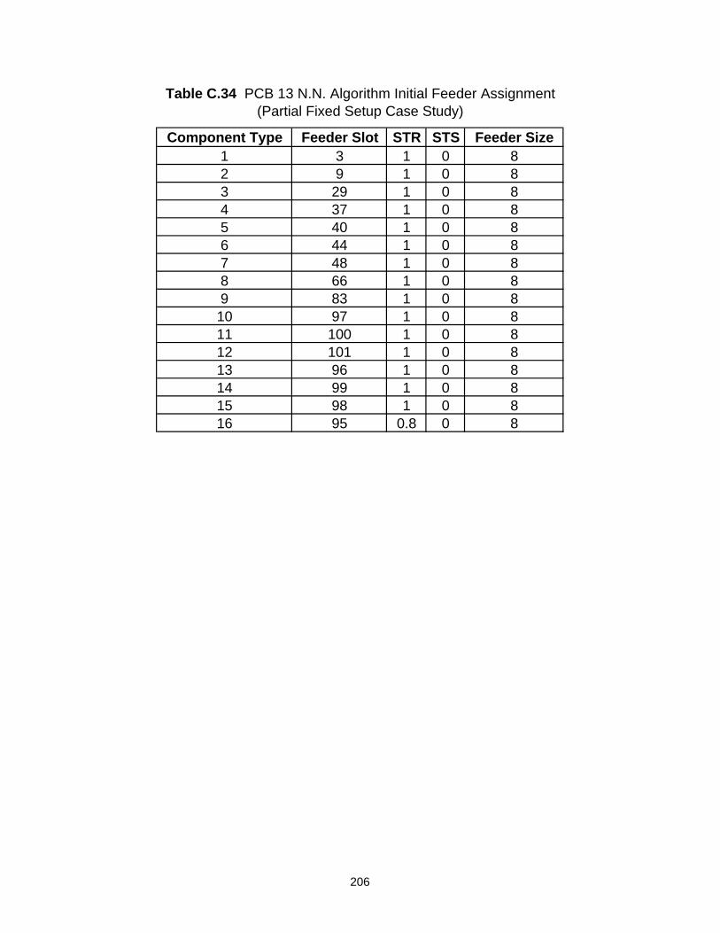
Table C.34 PCB 13 N.N. Algorithm Initial Feeder Assignment(Partial Fixed Setup Case Study)
Component Type Feeder Slot STR STS Feeder Size1 3 1 0 82 9 1 0 83 29 1 0 84 37 1 0 85 40 1 0 86 44 1 0 87 48 1 0 88 66 1 0 89 83 1 0 810 97 1 0 811 100 1 0 812 101 1 0 813 96 1 0 814 99 1 0 815 98 1 0 816 95 0.8 0 8
206

Table C.35 PCB 13 N.N. Algorithm Improved Component Placement Sequence(Partial Fixed Setup Case Study)
Component Type STR STS X-Location Y-Location Feeder Slot1 1 0 -7.85 68.45 31 1 0 -24.96 55.12 31 1 0 -87.19 52.58 32 1 0 -119.24 87.51 95 1 0 -128.95 87.99 403 1 0 -126.56 102.75 293 1 0 -118.94 102.75 293 1 0 -120.84 102.75 293 1 0 -122.75 102.75 293 1 0 -124.65 102.75 293 1 0 -160.06 86.24 293 1 0 -149.09 95.28 294 1 0 -144.97 103.23 374 1 0 -129.25 79.1 375 1 0 -150.06 76.41 406 1 0 -157.52 86.72 447 1 0 -120.21 94.49 487 1 0 -120.21 91.95 487 1 0 -120.21 89.41 487 1 0 -120.21 97.03 488 1 0 -144.97 104.65 668 1 0 -154.35 87.35 668 1 0 -288.79 51.31 669 1 0 -288.48 54.82 839 1 0 -160.7 77.98 839 1 0 -160.7 74.32 839 1 0 -145.13 100.36 839 1 0 -130.37 103.38 8316 0.8 0 -125.59 77.04 9513 1 0 -156.41 75.77 9612 1 0 -135.3 93.55 10111 1 0 -146.4 91.16 10014 1 0 -147.18 81.49 9910 1 0 -152.6 92.58 9810 1 0 -154.17 75.14 9815 1 0 -292.6 54.82 97
9.54845933320Solution Time:
Component Placement Time (sec.):
207

Table C.36 PCB 13 N.N. Algorithm Improved Feeder Assignment(Partial Fixed Setup Case Study)
Component Type Feeder Slot STR STS Feeder Size1 3 1 0 82 9 1 0 83 29 1 0 84 37 1 0 85 40 1 0 86 44 1 0 87 48 1 0 88 66 1 0 89 83 1 0 810 98 1 0 811 100 1 0 812 101 1 0 813 96 1 0 814 99 1 0 815 97 1 0 816 95 0.8 0 8
208

209
VITA
Fernando Jose Vittes was born to Pedro and Ana Maria Vittes on February 28, 1975, in
Madrid, Spain. He was raised in Lima, Peru, and graduated from Liceo Naval Almirante
Guise High School in 1991.
Fernando enrolled at the Montgomery County Community College in Blue Bell,
Pennsylvania and later moved to Fairfax, Virginia and transferred to the Northern
Virginia Community College. At these institutions he studied two years of general
engineering and obtained the George L. Buck Award for most outstanding academic
achievement in engineering sciences at the Northern Virginia Community College.
In 1995, Fernando transferred to Virginia Polytechnic Institute and State University to
pursue the Bachelor of Science degree in Industrial and Systems Engineering. In 1996,
he was awarded the Marvin H. Agee Scholarship for outstanding academic achievement
in Industrial and Systems Engineering. He also graduated Summa Cum Laude as the
Class Valedictorian for the Class of Industrial and Systems Engineering, 1997.
Fernando proceeded to pursue the degree of Master of Science in the Manufacturing
Systems option of Industrial and Systems Engineering at Virginia Polytechnic Institute
and State University soon after obtaining the Bachelor’s degree. While pursuing his
degree, he worked as a graduate research assistant in three collaborative projects with
Ericsson, Inc. He was awarded the Master of Science degree in 1999.
Fernando has accepted a position as an Applications Engineer for i2 Technologies, Inc., a
leading consulting firm in supply chain management.


