
PAH Background Study and Calculation of
Background Threshold Values (DE-1348)
New Castle, Kent, and Sussex Counties, Delaware
Prepared for:
Delaware Department of Natural Resources and Environmental Control
Site Investigation and Restoration Section
391 Lukens Drive
New Castle, Delaware 19720
Prepared by:
EA Engineering, Science, and Technology, Inc., PBC
1311 Continental Drive, Suite K
Abingdon, Maryland 21009
January 2016
Version: FINAL Revision 1
EA Project No. 1482626

This page intentionally left blank

EA Project No.: 1482626
Version: FINAL Rev. 1
Page i
EA Engineering, Science, and Technology, Inc., PBC January 2016
New Castle, Kent, and Sussex Counties, Delaware PAH Background Study and Calculation of
Background Threshold Values (DE-1348)
TABLE OF CONTENTS
Page
LIST OF TABLES ......................................................................................................................... iii LIST OF FIGURES ....................................................................................................................... iii ACRONYMS AND ABBREVIATIONS ...................................................................................... iv
INTRODUCTION .............................................................................................................. 1
DEVELOPMENT AND IMPLEMENTATION OF PAH BACKGROUND
THRESHOLD VALUES BY OTHER REGULATORY AGENCIES .............................. 3
2.1 PROCESS, CIRCUMSTANCES, AND CRITERIA FOR CONDUCTING
SITE-SPECIFIC BACKGROUND STUDY, SAMPLE DESIGN, AND
STATISTICS .......................................................................................................... 3 2.2 SUMMARY OF STATE-SPECIFIC PAH BACKGROUND
CONCENTRATIONS ............................................................................................ 4
2.2.1 California .....................................................................................................4 2.2.2 Illinois ..........................................................................................................5
2.2.3 Massachusetts ..............................................................................................5 2.2.4 Maine ...........................................................................................................5 2.2.5 Washington State .........................................................................................6
2.3 SUMMARY ............................................................................................................ 6
EVALUATION OF AVAILABLE BACKGROUND DATA FOR PAHS IN
DELAWARE ...................................................................................................................... 7
3.1 COMPARABILITY OF THE 2011 AND 2014 DATA SETS ............................... 7
3.1.1 Study Design Comparability ........................................................................7 3.1.2 Data Comparability ......................................................................................8
3.2 SUMMARY OF BACKGROUND AREAS .......................................................... 8
CALCULATION OF BACKGROUND STATISTICS ................................................... 11
4.1 SUMMARY STATISTICS AND OUTLIER EVALUATION ............................ 11
4.2 STATISTCIAL METHODS FOR POTENTIAL BACKGROUND
THRESHOLD VALUES ...................................................................................... 15 4.3 STATISTICAL RESULTS ................................................................................... 18
IMPLEMENTATION OF THE BACKGROUND STATISTICS ................................... 21
5.1 COMPARISONS TO BACKGROUND THRESHOLD VALUES ..................... 21

EA Project No.: 1482626
Version: FINAL Rev. 1
Page ii
EA Engineering, Science, and Technology, Inc., PBC January 2016
New Castle, Kent, and Sussex Counties, Delaware PAH Background Study and Calculation of
Background Threshold Values (DE-1348)
5.2 HYPOTHESIS TESTING .................................................................................... 21
CONCLUSIONS............................................................................................................... 23
REFERENCES ................................................................................................................. 25
APPENDIX A: LOGNORMAL Q-Q PLOTS OF DETECTED PAHS FOR THE 2012 AND
2014 SOIL BACKGROUND STUDIES
APPENDIX B LOGNORMAL Q-Q PLOTS OF DETECTED PAHS OF THE COMBINED
2012 AND 2014 SOIL BACKGROUND STUDIES
APPENDIX C: BACKGROUND SITES AND SAMPLE LOCATIONS: 2014 STUDY
APPENDIX D: PAH BACKGROUND STUDY RAW AND REDUCED DATASETS
(PROVIDED AS AN EXCEL FILE)
APPENDIX E: PROUCL OUTPUTS
APPENDIX F: PAH BACKGROUND STUDY DATASET APPROPRIATE FOR
DISTRIBUTION (PROVIDED AS AN EXCEL FILE)

EA Project No.: 1482626
Version: FINAL Rev. 1
Page iii
EA Engineering, Science, and Technology, Inc., PBC January 2016
New Castle, Kent, and Sussex Counties, Delaware PAH Background Study and Calculation of
Background Threshold Values (DE-1348)
LIST OF TABLES
Number Title
1 Background Areas and Study Site Numbers
2 General Statistics of PAH Concentrations in Soil Samples
3 Computed Background Threshold Values for Detected PAH Concentrations in
Soil
4 Proposed Background Threshold Values for PAHs in Soil
LIST OF FIGURES
Number Title
1 Geologic Provinces and Reference Area Locations
2 Box Plot Analysis of Detected High Molecular Weight PAHs
3 Box Plot Analysis of Detected Low Molecular Weight PAHs
4 Decision Tree for Determining 95% Upper Simultaneous Limit (USL) from
PAH Monitoring Data Containing Both Detected and Nondetected Results.

EA Project No.: 1482626
Version: FINAL Rev. 1
Page iv
EA Engineering, Science, and Technology, Inc., PBC January 2016
New Castle, Kent, and Sussex Counties, Delaware PAH Background Study and Calculation of
Background Threshold Values (DE-1348)
ACRONYMS AND ABBREVIATIONS
BTV Background threshold value
CERCLA Comprehensive Environmental Response, Compensation, and Liability Act
CV Coefficient of variation
DNREC Delaware Department of Natural Resources and Environmental Control
EA EA Engineering, Science, and Technology, Inc., PBC
EPA United States Environmental Protection Agency
Ho Null hypothesis
Ha Alternative hypothesis
HSCA Hazardous Substance Cleanup Act
KM Kaplan-Meier
mg/kg Milligrams per kilograms
MDL Method detection limit
MVT Multivariate trimming
PAH Polycyclic aromatic hydrocarbon
Q-Q Plot Quantile-quantile plot
RL Reporting limit
SIRS Site Investigation and Restoration Section
SWFPR Site-wide false positive error rate
TACO Tiered Approach to Corrective Action Objectives
TCL Target compound list
UCL Upper confidence level
UPL Upper prediction limit
USL Upper simultaneous limit
UTL Upper tolerance level
UTL95-95 95% upper tolerance level with 95% confidence
VSP Visual Sample Plan

EA Project No.: 1482626
Version: FINAL Rev. 1
Page 1
EA Engineering, Science, and Technology, Inc., PBC January 2016
New Castle, Kent, and Sussex Counties, Delaware PAH Background Study and Calculation of
Background Threshold Values (DE-1348)
INTRODUCTION
EA Engineering, Science, and Technology Inc., PBC (EA) has been tasked by the Delaware
Department of Natural Resources and Environmental Control (DNREC) Site Investigation and
Restoration Section (SIRS) to conduct an evaluation of background polycyclic aromatic
hydrocarbon (PAH) concentrations found throughout Delaware (DE-1348) and to calculate
background statistics. This work is a continuation of the effort completed by EA in 2014 (EA
2014). In addition to the evaluation of background PAH concentrations and calculation of
background statistics, this document includes a summary of how other regulatory agencies
identify and use PAH background statistics.
DNREC-SIRS administers site cleanup programs for the State of Delaware under the Hazardous
Substance Cleanup Act (HSCA). Some chemicals regulated by the program are present in soil as
a natural condition or as the result of human activities. PAHs are widely present in soils due to
industrial activities resulting in releases, as defined by HSCA. However, PAHs are also believed
to be present in soil where no specific release has occurred due to natural causes (e.g., fire) or
due to ubiquitous, anthropogenic impacts. Ubiquitous, anthropogenic impacts result in an
ambient condition and are the result of deposition of PAH particles originating from sources such
as asphalt. These impacts can be considered background. DNREC-SIRS has developed the
following definition of background as it relates to efforts at sites regulated under HSCA
(DNREC 2015).
The concentration of substances widely present in the soil, sediment, air, surface water or
groundwater in the vicinity of a facility, or at a comparable reference area, due to
natural causes or human activities other than releases from, or activities on, the facility,
as determined by the Department.
In the context of DNREC-SIRS’ efforts under HSCA, the identification of background levels of
PAHs would be used to assist in the determination of whether or not no further investigation or
cleanup actions for these constituents would be required at a HSCA site.

EA Project No.: 1482626
Version: FINAL Rev. 1
Page 2
EA Engineering, Science, and Technology, Inc., PBC January 2016
New Castle, Kent, and Sussex Counties, Delaware PAH Background Study and Calculation of
Background Threshold Values (DE-1348)
This page intentionally left blank

EA Project No.: 1482626
Version: FINAL Rev. 1
Page 3
EA Engineering, Science, and Technology, Inc., PBC January 2016
New Castle, Kent, and Sussex Counties, Delaware PAH Background Study and Calculation of
Background Threshold Values (DE-1348)
DEVELOPMENT AND IMPLEMENTATION OF PAH BACKGROUND
THRESHOLD VALUES BY OTHER REGULATORY AGENCIES
All other state environmental departments have been examined to characterize the following with
respect to the determination of background values or providing general state background values,
specifically for PAHs:
The process, circumstances, and criteria (quantitative and qualitative) for conducting a
site-specific background study
Sample designs used to generate data
Calculation of Background Threshold Values (BTVs) for PAHs
Calculation of site-specific background values.
2.1 PROCESS, CIRCUMSTANCES, AND CRITERIA FOR CONDUCTING SITE-
SPECIFIC BACKGROUND STUDY, SAMPLE DESIGN, AND STATISTICS
Most state agencies acknowledge that background or reference concentrations can play a role in
state decisions (typically for Brownfield Sites). However, most states did not provide specific
guidance on how to conduct a site-specific background study or how to develop state- or area-
specific background values. An exception is Missouri, which has a short document that
describes how to conduct a background study (Appendix M to their Risk-Based Corrective
Action Technical Guidance [MODNR 2015]). This document notes that background samples
should be collected from an area with a soil type similar to that found at the site, but the
document does not provide guidance with respect to numbers of samples or appropriate
statistical analyses. Approval of the study by the state is required.
Similarly, in 1994 the Michigan Department of Natural Resources published a guidance
document for how to conduct a background study (MIDNR 1994). The document offers some
advice for establishing random grids for sampling purposes; however, because it is an older
document, it only offers the now outdated “background plus three standard deviations” approach
as the recommendation for BTVs. In 2005, Michigan published a background soil survey for
metals, but has not addressed PAHs (MIDNR 2005).
In summary the guidance offered by states for conducting background studies is limited. Most
states indicate that consideration of background data is acceptable for decision-making, but offer
little guidance for how to generate such data, establish sampling designs, or calculate BTVs. In
addition, because the statistical assessment of background data has advanced considerably since
the 1990s, recommended statistical treatments vary widely, from three times the standard
deviation, and the 90th or the 95th percentile upper confidence limit (UCL), to the more recently
promoted upper prediction limit (UPL) and upper tolerance limit (UTL).

EA Project No.: 1482626
Version: FINAL Rev. 1
Page 4
EA Engineering, Science, and Technology, Inc., PBC January 2016
New Castle, Kent, and Sussex Counties, Delaware PAH Background Study and Calculation of
Background Threshold Values (DE-1348)
While state-specific guidance on the development of background studies is limited, the United
States Environmental Protection Agency (EPA) has published a guidance document specifically
discussing the characterization of background concentrations in soil and how to evaluate
background datasets in comparison to site-specific data (EPA 2002). This document was
prepared to support efforts at Comprehensive Environmental Response, Compensation, and
Liability Act (CERCLA) sites, and the concepts and statistical tools described in the guidance
can be applied to HSCA sites as well. The EPA (2002) guidance document discusses in detail
the following aspects of a background study:
Selection of background areas that take into account soil types, the physical and chemical
nature of the contaminants of concern, and potential anthropogenic impacts (if any) at
selected background sample locations
Sample sizes necessary to derive background concentrations (a minimum of 5, 20 or
greater preferred) and statistical tests that can be used to estimate the necessary number
of background samples
Data quality objectives appropriate to a background study including discussions about
sample depths, proximity to potential anthropogenic sources, and appropriate if-then
decision statements
Preliminary data analysis tools such as tests for normality, graphical displays of data (like
the quantile plots shown in Appendixes A and B of this document), and the identification
of outliers (Section 4.1 of this document)
Statistical tools for the comparison of background and site data including parametric and
nonparametric (e.g. Wilcoxon Rank Sum) tests and hypothesis testing.
The background study presented herein for PAHs in Delaware, and the statistical tools employed
for the calculation of candidate BTVs, are consistent with the EPA guidance.
2.2 SUMMARY OF STATE-SPECIFIC PAH BACKGROUND CONCENTRATIONS
Five states provided some kind of PAH background data, which are summarized below.
2.2.1 California
In 2009, the California Department of Toxic Substances Control published benzo(a)pyrene
equivalents background values for northern and southern California (Cal DTSC 2009).
California Toxicity Equivalency Factors were used in the assessment. The guidance is geared to
the assessment of historic manufactured gas sites (which are notorious for their PAH
contamination). Large numbers of samples were involved (86 for northern California and 185
for southern California), and 95% UCLs and UTLs were reported for benzo(a)pyrene equivalents
to assist in the determination of nature and extent of contamination. UTLs for northern and
southern California for benzo(a)pyrene equivalents were 1.5 and 0.9 milligrams per kilograms

EA Project No.: 1482626
Version: FINAL Rev. 1
Page 5
EA Engineering, Science, and Technology, Inc., PBC January 2016
New Castle, Kent, and Sussex Counties, Delaware PAH Background Study and Calculation of
Background Threshold Values (DE-1348)
(mg/kg) respectively. Raw data (in Excel format) from these data-sets are available for
download for statistical comparisons to site data.
2.2.2 Illinois
Illinois has established Tiered Approach to Corrective Action Objectives (TACO) values for use
in their voluntary cleanup program (ILEPA 2015). Many TACO screening values are based on
risk; however, TACO screening values for PAHs (specifically benzo(a)pyrene) have been
established based on background concentrations. Four separate benzo(a)pyrene values have been
established:
Within the Chicago corporate limits, 1.3 mg/kg
A populated area within a Metropolitan Statistical Area excluding Chicago, 2.1 mg/kg
A populated area not in a Metropolitan Statistical Area, 0.98 mg/kg
Outside a populated area, 0.09 mg/kg.
These concentrations have been tied to the Illinois Administrative Code (35 IAC 742 Appendix
A, Table H); which provides background values for PAHs in Chicago, metropolitan areas other
than Chicago, and non-metropolitan areas. It is not clear how these background PAH
concentrations have been derived, and raw data have not been provided; consequently, statistical
hypothesis testing cannot be performed. TACO guidance in the Administrative Code (35 IAC
742) offers very generic guidance on how to establish background, relying on concurrence with
the regulators.
2.2.3 Massachusetts
Massachusetts established background values for PAHs based on existing data sets (MADEP
2002). Background levels were established at the 90th percentile of all background values for
“natural” soil and soils containing coal or wood ash as “fill material.” From the documentation,
it does not appear as though any outlier tests were performed on these data. The raw data have
not been made available to the public; thus statistical hypothesis testing cannot be performed.
2.2.4 Maine
In 2012, Maine published background concentrations of PAHs in soils (MEDEP 2012). Data
were generated from Brownfield sites and studies performed by the State. Two sets of results
were produced, urban and rural, the former based on areas designated by the Maine Department
of Transportation to be Urban Compact Areas or “built-up” sections of road where structures
along the highway are nearer than 200 feet apart for a distance of 1/4 of a mile. One observation
made was that the urban soil dataset had two separate distributions, one associated with urban fill
and the other with urban soil. Urban fill was handled separately from urban soil. These data
were examined for outliers (box and whisker plots followed by interquartile range testing), and
then by tests for single/multiple populations. Once the outliers were removed, 90% UPLs were
calculated for urban and rural PAHs using ProUCL. Finally, the raw data are available for
statistical testing purposes.

EA Project No.: 1482626
Version: FINAL Rev. 1
Page 6
EA Engineering, Science, and Technology, Inc., PBC January 2016
New Castle, Kent, and Sussex Counties, Delaware PAH Background Study and Calculation of
Background Threshold Values (DE-1348)
2.2.5 Washington State
Washington State has published a background study of arsenic, PAHs, and dioxin/furans for
rural state parks (WSDOE 2011). The study was based on 41 6-point composite samples from
31 rural parks and 1 undeveloped area. Sample areas were remote by design; none were within
city or town boundaries, they were miles from major roads, and were in areas with population
densities less than 500 people per square mile. The only study area description noted was
whether the samples were from a forested or open area. Outlier testing was completed, with box
and whisker plots followed by Principal Component Analysis and other robust outlier testing
techniques. For PAHs, the carcinogenic toxic equivalents relative to benzo(a)pyrene were
calculated for each sample. Statistics presented include percentiles and other data; however,
UCLs, UPLs, or UTLs were not presented. Separate values were presented for forested and open
areas. These data show very low PAH concentrations due to the sample design focusing on rural
State parks.
2.3 SUMMARY
Most states accept background as an appropriate consideration for decision-making, although
few offer specific guidance for how to design, conduct, and analyze these types of data. Five
states were found to have published some type of PAH background values. Of all the states
included in this list, the state of Maine has the most recent and robust assessment. EPA has
published a detailed guidance document for the characterization of background concentrations in
soil and the evaluation of background datasets in comparison to site-specific data. The
background study discussed herein for Delaware, and the statistical tools employed for the
calculation of candidate BTVs, are consistent with the EPA (2002) guidance.

EA Project No.: 1482626
Version: FINAL Rev. 1
Page 7
EA Engineering, Science, and Technology, Inc., PBC January 2016
New Castle, Kent, and Sussex Counties, Delaware PAH Background Study and Calculation of
Background Threshold Values (DE-1348)
EVALUATION OF AVAILABLE BACKGROUND DATA FOR PAHS IN
DELAWARE
In 2012, DNREC-SIRS completed a statewide background soil study of PAHs and metals in an
attempt to establish background levels to compare to levels at HSCA sites (DNREC 2012). This
study focused on rural/suburban areas with no history of industrial use, development, or
suspected contamination. The background study was later expanded to include the collection of
samples in urban areas as well as rural/residential areas (EA 2014). A total of eight
rural/suburban background areas were included in the 2012 effort and 12 areas (six urban and six
rural/suburban) were included in the expanded (2014) effort. The same rural/suburban areas
were sampled as part of both efforts; although, the specific sampling sites may have changed.
Background areas were dispersed among two geologic provinces and the three counties of the
State. The selection of the background areas for the 2012 effort is detailed in DNREC 2012 and
the selection of background areas for the expanded effort is detailed in EA 2013a, 2013b, and
2014.
3.1 COMPARABILITY OF THE 2011 AND 2014 DATA SETS
The two available datasets were evaluated for comparability to determine whether or not they
could be combined into a single dataset for statistical evaluation. The evaluation included a
qualitative assessment of the study designs and methods and a quantitative assessment of the
datasets.
3.1.1 Study Design Comparability
The 2012 study identified eight rural/suburban areas that did not have any prior commercial or
industrial uses or recent agricultural uses (as confirmed through interviews with Wildlife
Managers and Park Managers). Six of these background areas were selected by DNREC-SIRS
for re-evaluation in the expanded (2014) background study. Six urban background areas were
also identified for evaluation in the expanded study after completion of a brief site history search,
which confirmed that none of them had been part of a current or past state or federal cleanup,
and that there were no other reasons to believe the area might contain PAHs from a historic, on-
site release (EA 2013a).
For both efforts, DNREC-SIRS identified two-acre plots within each background area to be
sampled. The two-acre plots were referred to as “background study sites.” The two-acre plots
identified for the 2014 study were randomly selected through the use of Visual Sample Plan
(VSP) software (VSP Development Team 2013) with some restrictions to avoid large areas
where sampling would not be possible (e.g., impervious areas and ponds) (EA 2013b). The
method employed for the selection of the two-acre plots sampled as part of the 2012 effort is not
detailed in DNREC (2012).
For the 2012 study, 20 sample locations were fixed at each two-acre background study site on a
systematic rectangular grid with a random start. For the 2014 study, the 20 sample locations
were identified with VSP using a triangular systematic grid with a random start. For both

EA Project No.: 1482626
Version: FINAL Rev. 1
Page 8
EA Engineering, Science, and Technology, Inc., PBC January 2016
New Castle, Kent, and Sussex Counties, Delaware PAH Background Study and Calculation of
Background Threshold Values (DE-1348)
studies, surface soil samples were collected from the top 6-inches of soil in accordance with the
DNREC-SIRS Standard Operating Procedure for soil sampling. Samples were analyzed by
DNREC-SIRS contracted laboratories for target compound list PAHs via method SW846
Method 8270.
The methods used to select background areas and sampling locations, and the sample collection
and analytical methods employed for both the 2012 and the 2014 background studies were
similar. Therefore, the two studies would be expected to yield comparable data.
3.1.2 Data Comparability
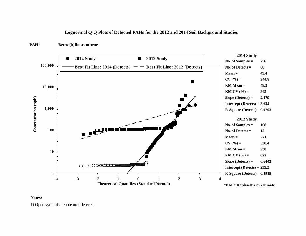
Lognormal quantile-quantile plots (Q-Q plots) of detected PAHs were prepared to evaluate the
comparability of the 2012 dataset and the 2014 dataset. The Q-Q plots are presented in Appendix A for
each PAH with at least one detected sample result; values for non-detects (i.e., “U” qualified) were set to
the method detection limit (MDL). The Q-Q plots show that a portion of the 2012 dataset is confounded
by non-detect results having an erroneously high MDL due to laboratory error. Therefore, non-detect
results in the 2012 study that had a MDL exceeding the maximum MDL of the 2014 study were treated
as rejected data and were not included in any further analysis. Lognormal Q-Q plots of the combined
2012/2014 datasets were then developed in order to investigate the distribution of detected results and to
identify potential outliers. The Q-Q plots of the combined datasets are presented in Appendix B, and are
further discussed in Section 4.
3.2 SUMMARY OF BACKGROUND AREAS
The selection of the background areas and background study sites for the 2014 study is
summarized in Section 3.1.1. The specific background areas and background study sites
sampled as part of the 2014 study, and therefore contributing to the dataset used to generate
BTVs, are identified below. Twelve background areas were included in the 2014 effort. Four
areas were located in each of Delaware’s counties; two rural/suburban areas and two urban areas
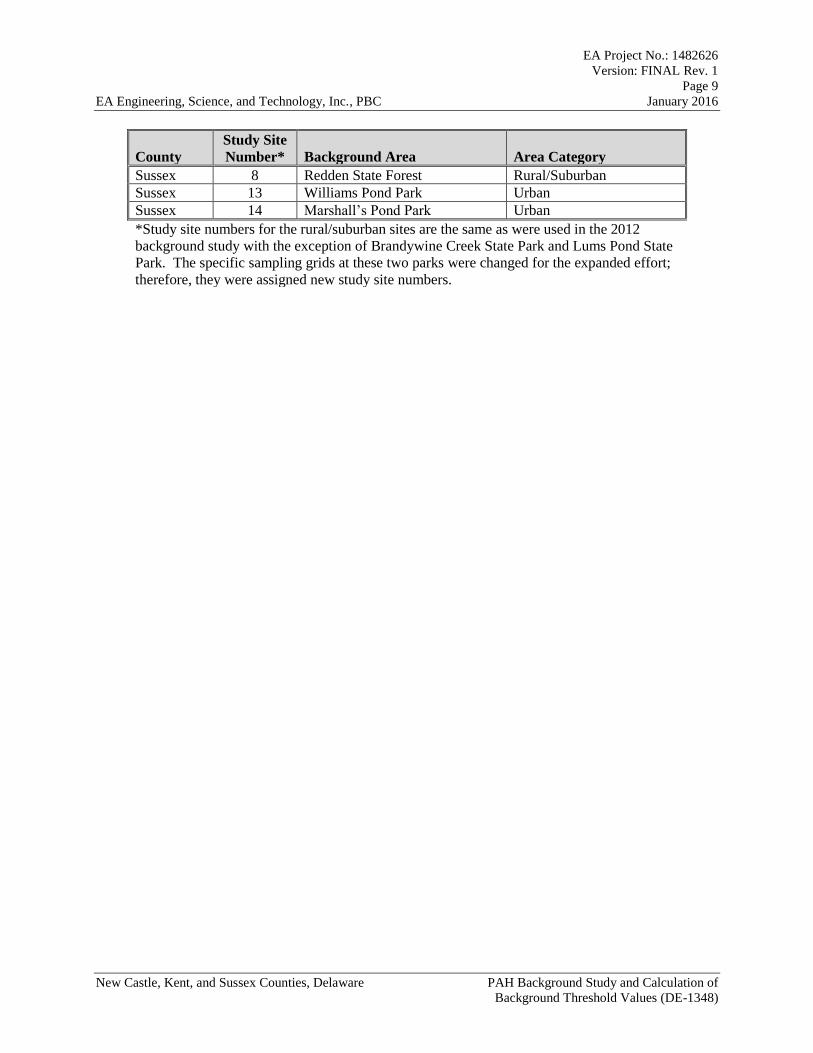
were selected for each county. The background areas are identified in Table 1 and their locations
are presented in Figure 1. Appendix C includes sampling coordinates and sample location
figures for each of the background study sites.
Table 1. Background Areas and Study Site Numbers
County
Study Site
Number* Background Area Area Category
New Castle 16 Brandywine Creek State Park Rural/Suburban
New Castle 15 Lums Pond State Park Rural/Suburban
New Castle 9 Banning Park Urban
New Castle 10 Bellevue State Park Urban
Kent 5 Norman Wilder Wildlife Area Rural/Suburban
Kent 6 Norman Wilder Wildlife Area Rural/Suburban
Kent 11 Smyrna Municipal Park Urban
Kent 12 Brecknock Park Urban
Sussex 7 Redden State Forest Rural/Suburban
EA Project No.: 1482626
Version: FINAL Rev. 1
Page 9
EA Engineering, Science, and Technology, Inc., PBC January 2016
New Castle, Kent, and Sussex Counties, Delaware PAH Background Study and Calculation of
Background Threshold Values (DE-1348)
County
Study Site
Number* Background Area Area Category
Sussex 8 Redden State Forest Rural/Suburban
Sussex 13 Williams Pond Park Urban
Sussex 14 Marshall’s Pond Park Urban
*Study site numbers for the rural/suburban sites are the same as were used in the 2012
background study with the exception of Brandywine Creek State Park and Lums Pond State
Park. The specific sampling grids at these two parks were changed for the expanded effort;
therefore, they were assigned new study site numbers.

New Castle County
Kent County
Sussex County Williams Pond ParkSite 13
Banning ParkSite 9
Brecknock ParkSite 12
Marshalls Pond ParkSite 14
Bellevue State ParkSite 10
Lums Pond State ParkSite 15
Smyrna Municipal ParkSite 11
Brandywine Creek State ParkSite 16
Redden State ForestSite 8
Redden State ForestSite 7
Norman G. Wilder Wildlife AreaSites 5 and 6
Figure 1Figure 1Geologic Provinces andGeologic Provinces and
Reference Area LocationsReference Area Locations
\\abin
gdon
\proje
cts\U
nivers
al GI
S\DNR
EC\M
XD\PA
H St
udy\1
_Site
Loca
tions
.mxd
0 105 Miles
LegendBackground Study SiteCounty Boundaries
Physiographic ProvinceCoastal PlainPiedmont
Data Sources:Delaware Geospatial Data Exchange, 2013Delaware Geological Survey, 2013
P A H B a c k g r o u n d S t u d yP A H B a c k g r o u n d S t u d yNew Castle, Kent, and
Sussex Counties, Delaware

EA Project No.: 1482626
Version: FINAL Rev. 1
Page 11
EA Engineering, Science, and Technology, Inc., PBC January 2016
New Castle, Kent, and Sussex Counties, Delaware PAH Background Study and Calculation of
Background Threshold Values (DE-1348)
CALCULATION OF BACKGROUND STATISTICS
EPA guidance (EPA 1989, 2002, 2013) specifies that upper limits such as the UPL, UTL, or
upper simultaneous limit (USL) be used for calculating the BTV. These upper limits represent a
high estimate of background concentrations, such that PAH concentrations from natural or
ubiquitous anthropogenic sources are unlikely to exceed them (i.e., a low rate of false positives is
expected). BTVs would most likely be used for screening individual data points that are part of
small sampling populations (e.g., a soil sample’s data from a given source area). Hypothesis
testing may be conducted as an alternative for larger datasets (e.g., soil sampling data from an
entire site), as discussed in Chapter 5.
4.1 SUMMARY STATISTICS AND OUTLIER EVALUATION
In general, the frequency of detection of PAHs was low. PAHs were detected with greater
frequency at four sites, Smyrna Municipal Park, Norman Wilder Wildlife Area Site 5, Williams
Pond Park, and Marshall’s Pond Park. In addition, high molecular weight PAHs tended to have
higher frequencies of detection than low molecular weight PAHs (acenaphthene, acenaphthylene,
anthracene, fluoranthene, indeno(1,2,3-c,d)pyrene, and phenanthrene).
Table 2 presents summary statistics for the surface soil dataset. The full, raw dataset is provided
in Appendix D. The following general statistics were computed using ProUCL:
Number of samples
Number of detected samples
Minimum and maximum non-detect result
Minimum and maximum detected result
Kaplan-Meier mean and standard deviation assuming a normal distribution.
Box-and-whisker plots (Figures 2 and 3) were prepared and present the 25th percentile, median,
and 75th percentile of the full, raw dataset for each PAH with at least one detected sample result,
and non-detects set to the MDL. The whiskers indicate the 5th and 95th percentiles, and detected
sample results exceeding the 95th percentile are identified.

EA Engineering, Science, and Technology, Inc., PBC
EA Project No.: 1482626Version: FINAL Rev. 1
January 2016
Table 2. General Statistics of PAH Concentrations in Soil Samples
PAH Units MDL RLNo. of
Samples
No. of Samples Detected
Above MDL
Minimum Value of Dataset
Maximum Value of Dataset
Minimum Detected Value1
Maximum Detected
ValueKM
Mean2KM Std.
Dev. 2
2-chloronaphthalene µg/kg 41 370 240 0 < 38 < 54 NC NC NC NC2-methylnaphthalene µg/kg 47 370 240 0 < 44 < 63 NC NC NC NCAcenaphthene µg/kg 54 370 246 2 < 3 1,500 75 1,500 < 9.38 95.3Acenaphthylene µg/kg 43 370 246 3 < 1 510 79 510 < 4.4 36.3Anthracene µg/kg 45 370 253 7 < 1 2400 67 2400 < 16.1 158Benzo[a]anthracene µg/kg 2.6 37 262 55 < 2 720 5 720 27.1 88.4Benzo[a]pyrene µg/kg 2.6 37 258 83 < 2 210 4 210 19.3 39.5Benzo[b]fluoranthene µg/kg 2.3 37 238 79 < 2.2 240 6 240 24 48.5Benzo[g,h,i]perylene µg/kg 27 370 259 38 < 2 2100 37 2100 47.9 214Benzo[k]fluoranthene µg/kg 2.8 37 256 49 < 2.8 700 4 700 22.4 76.8Chrysene µg/kg 43 370 262 39 < 43 990 58 990 < 35.2 124Dibenz[a,h]anthracene µg/kg 4.6 37 253 30 < 2 2700 8 2700 24.3 181Fluoranthene µg/kg 49 370 267 36 < 2 1200 76 1200 < 41.7 149Fluorene µg/kg 47 370 245 2 < 5 490 74 490 < 7.26 31.2Indeno[1,2,3-c,d]pyrene µg/kg 6.8 37 258 54 < 2 2200 10 2200 48.4 209Naphthalene µg/kg 43 370 255 2 < 2 210 190 210 <43 17.5Phenanthrene µg/kg 47 370 257 18 < 47 430 63 430 < 12 48.1Pyrene µg/kg 31 370 269 56 < 31 1200 42 1200 47.2 1561. Minimum detected value that is greater than the MDL presented in this table. < = Value is less than the MDL2. Computed using Kaplan-Meier (KM) estimator. PAH = Polycyclic aromatic hydrocarbonKM = Kaplan-Meier RL = Reporting limitMDL = Minimum detection limit Std. Dev. = Standard deviationNC = Not calculated; analyte was not detected in any samples µg/kg = Micrograms per kilogram
New Castle, Kent, and Sussex Counties, Delaware PAH Background Study and Calculation of Background Threshold Values (DE-1348)

1
10
100
1000
10000
100000
Soil
Con
cent
ratio
n (
g/kg
)
Figure 2. Box plot analysis of detected high molecular weight PAHs.Boxes show 25th percentile, median, and 75th percentile of the data. The whiskers indicate the 5th and 95th percentiles. Detected sample results exceeding the 95th percentile are shown as symbols ).

1
10
100
1000
10000
100000
Soil
Con
cent
ratio
n (
g/kg
)
Figure 3. Box plot analysis of detected low molecular weight PAHs.Boxes show 25th percentile, median, and 75th percentile of the data. The whiskers indicate the 5th and 95th percentiles. Detected sample results exceeding the 95th percentile are shown as symbols ).

EA Project No.: 1482626
Version: FINAL Rev. 1
Page 15
EA Engineering, Science, and Technology, Inc., PBC January 2016
New Castle, Kent, and Sussex Counties, Delaware PAH Background Study and Calculation of
Background Threshold Values (DE-1348)
Q-Q plots were also prepared for each detected PAH. The Q-Q plots are presented in Appendix
B. The box-and-whisker and Q-Q plots show that the distributions of PAH concentrations are
positively skewed, indicting the presence of potential outliers or mixed-population data sets that
are not representative of background. Therefore, an outlier evaluation was conducted to identify
and remove potential outliers prior to computing USLs. Outliers were identified using
multivariate trimming (MVT), which is a robust outlier test suitable for identifying multiple
outliers in a dataset containing multiple outliers or sample data from more than one population
(EPA 2009). The MVT outlier analysis was conducted using the Scout 2008 version 1.0
software package (EPA 2009). Sample data exceeding the final squared Mahalanobis distance at
the 99% significance level were treated as statistical outliers, and removed from the background
dataset prior to computing USLs. Q-Q plots of the final background dataset are presented in
Appendix B. These Q-Q plots show the distribution of detected sample data plotted against the
quantiles of a theoretical lognormal distribution. The Q-Q plots also show the values and
theoretical quantiles of the outliers identified from the MVT outlier test. The final, reduced
dataset that was used for computing USLs is provided in Appendix D.
4.2 STATISTCIAL METHODS FOR POTENTIAL BACKGROUND THRESHOLD
VALUES
The following statistics were considered as potential BTV candidates: the 95% UPL, the 95%
UTL with 95% coverage, and the 95% USL.
A UPL represents the upper end of a range that is calculated to include one or more
independent observation from the same population with a specified confidence. For
example, a UPL with 95% confidence for background benzo(a)pyrene concentrations in
soil represents the concentration that a benzo(a)pyrene concentration from an
independent background sample will fall below that value with 95% confidence. UPLs
are commonly used as BTVs, but it should be noted that false positive error rate 𝛼 applies
to each comparison made to the UPL in a given study. Therefore, the site-wide false
positive error rate (SWFPR) for a given study increases with each comparison (𝑘:
𝑆𝑊𝐹𝑃𝑅 = 1 − (1 − 𝛼)𝑘 ). Therefore, using the UPL as a BTV can yield an
unacceptably high SWFPR for studies requiring many comparisons to the UPL.
A UTL is a statistical upper limit designed to contain a specified proportion of the
population with a specified confidence. For example, a 95% UTL with 95% (UTL95-95)
confidence represents the concentration at which there is 95% confidence that 95% of all
background benzo(a)pyrene concentrations will be below the value. The UTL95-95
exceeds the 95% UPL, but converges toward the 95% UPL as the number of samples in
the background data set increases. By definition the UTL95-95 can classify 5% of
background observations as not coming from the background population with a
confidence of 95%. Therefore, when comparing data to the UTL, the number of false
positive errors will increase with the number of comparisons made.

EA Project No.: 1482626
Version: FINAL Rev. 1
Page 16
EA Engineering, Science, and Technology, Inc., PBC January 2016
New Castle, Kent, and Sussex Counties, Delaware PAH Background Study and Calculation of
Background Threshold Values (DE-1348)
A USL is statistical upper limit designed to contain all of the population with a specified
confidence. The 95% USL represents a statistic such that all observations from the
background dataset will be less than or equal to the 95% USL with a confidence of 95%.
Therefore, assuming that the background data set is free of outliers, the computed 95%
USL will always be greater than or equal to the maximum value in the background
dataset. The false positive error rate does not change with the number of comparisons to
the USL; therefore, the USL is suitable for performing many comparisons
simultaneously. A potential disadvantage to using the USL as a BTV is that the USL can
yield a high false negative error rate if outliers are present in the background data set.
If a future observation exceeds the UPL, UTL, or USL, then there is statistical evidence that the
analyzed sample does not fit in the population of natural background concentrations, and likely
represents a sample from an impacted area. Because it is expected that the computed BTVs will
be compared to many individual sample concentrations from many future projects, the 95% USL
was chosen as the upper limit to be used for the BTV.
Technical guidance (EPA 2013) recommends that a minimum of 8 to 10 sample concentrations
be used to derive a BTV or conduct hypothesis tests with site data. The background dataset
evaluated for this study consisted of approximately 250 samples after removal of statistical
outliers as described in Section 4.1. The number of detected concentrations for individual PAHs
ranged from 0 to 83 (Table 2). For PAHs with at least 5 detected sample results, the 95% USL
was computed using the ProUCL software version 5.0 (EPA 2013). Because all of the PAH
datasets contained non-detect results, estimates of the mean and standard deviation were also
computed using the Kaplan-Meier method, which estimates the population mean and standard
deviation using a distribution function adjusted for censoring. The distribution of detected
results was characterized as normally distributed, gamma distributed, lognormally distributed, or
nonparametric. As summarized in Figure 4, upper limits were then computed using the Kaplan-
Meier method with an assumed data distribution consistent with the distribution of detected
results. Details of the numerical procedure used to compute upper limits using the Kaplan-Meier
method can be found in the ProUCL Technical Guide (EPA 2013). For detected PAHs with less
than 5 detected sample results, the maximum detected value was selected as a nonparametric
95% USL.

Figure 4. Decision tree for determining 95% upper simultaneous limit (USL) from PAH monitoring data containing both detected and nondetected results.
NO
Remove statistical outliers using multivariate trimming (MVT) at
99% significance levelDetected results are
normally distributed?
95% USL computed using Kaplan-Meier (KM) estimates assuming a
normal distribution
YES
Q-Q Plot shows evidence of potential
outliers?
Detected results are gamma distributed?
NO
YES95% USL computed using Kaplan-Meier (KM) estimates assuming a
Wilson Hilferty (WH) gamma distribution
Detected results are lognormally distributed?
NO
YES95% USL computed using Kaplan-Meier (KM) estimates assuming a
lognormal distribution
YES
NO
95% USL computed using higher order statistics

EA Project No.: 1482626
Version: FINAL Rev. 1
Page 18
EA Engineering, Science, and Technology, Inc., PBC January 2016
New Castle, Kent, and Sussex Counties, Delaware PAH Background Study and Calculation of
Background Threshold Values (DE-1348)
4.3 STATISTICAL RESULTS
The ProUCL outputs are presented in Appendix E. The outputs contain a variety of upper limit
statistics, including USLs, computed under different distribution assumptions. Table 3
summarizes the ProUCL outputs for each PAH and includes an appropriate 95% USL for each
PAH with at least 5 detected results. For statistical calculations, all detected results that were
less than the MDL presented in Table 2 were treated as non-detects. Table 4 presents a summary
of the computed BTVs, the target cancer risk and hazard quotient for each value, and the
proposed BTV. For those detected PAHs without sufficient detected results to compute
statistically based USLs, the maximum detected result was used as the BTV.
Most of the proposed BTVs are less than the EPA Region 3 human health residential soil
screening level with the exception of the following:
Benzo(a)anthracene
Benzo(a)pyrene
Benzo(b)fluoranthene
Dibenz(a,h)anthracene
Indeno(1,2,3-c,d)pyrene.

EA Engineering, Science, and Technology, Inc., PBC
EA Project No.: 1482626Version: FINAL Rev. 1
January 2016
Table 3. Computed Background Threshold Values for Detected PAH Concentrations in SoilUSL Computed with ProUCL
ProUCL Method 195% USL
Acenaphthene µg/kg 54 370 246 2 1,500 NC NCAcenaphthylene µg/kg 43 370 246 3 510 NC NCAnthracene µg/kg 45 370 253 7 2,400 KM-Normal 570Benzo[a]anthracene µg/kg 2.6 37 262 55 720 KM-Lognormal 819Benzo[a]pyrene µg/kg 2.6 37 258 83 210 KM-Gamma(WH) 242Benzo[b]fluoranthene µg/kg 2.3 37 238 79 240 KM-Gamma(WH) 1,106Benzo[g,h,i]perylene µg/kg 27 370 259 38 2,100 Nonparametric 2,100Benzo[k]fluoranthene µg/kg 2.8 37 256 49 700 KM-Gamma(WH) 345Chrysene µg/kg 43 370 262 39 990 Nonparametric 990Dibenz[a,h]anthracene µg/kg 4.6 37 253 30 2,700 KM-Logormal 166Fluoranthene µg/kg 49 370 267 36 1,200 KM-Logormal 1,045Fluorene µg/kg 47 370 245 2 490 NC NCIndeno[1,2,3-c,d]pyrene µg/kg 6.8 37 258 54 2,200 KM-Lognormal 1,304Naphthalene µg/kg 43 370 255 2 210 NC NCPhenanthrene µg/kg 47 370 257 18 430 KM-Gamma(WH) 138Pyrene µg/kg 31 370 269 56 1,200 KM-Gamma(WH) 3,505BTV = Background threshold value PAH = Polycyclic aromatic hydrocarbonCV = Coefficient of variation RL = Reporting limitKM = Kaplan-Meier USL = Upper simultaneous limitMDL = Minimum detection limit µg/kg = micrograms per kilogramNC = Not calculated; insufficient detected sample results
- KM-Normal = Kaplan-Meier estimates assuming normal distribution - KM-Lognormal = Kaplan-Meier estimates assuming lognormal distribution - KM-Gamma(WH) = Kaplan-Meier estimates assuming Wilson Hilferty (WH) gamma distribution - KM-Normal = Kaplan-Meier estimates assuming normal distribution
1. Statistical method for computing upper limits as recommended by ProUCL 5.0. Note that for statistical calculations, all detected results that were less than the MDL presented in Table 2 were treated as non-detects.
PAH Units No. of
Samples
No. of Samples Detected
Above MDLMax
DetectedMDL RL
New Castle, Kent, and Sussex Counties, Delaware PAH Background Study and Calculation of Background Threshold Values (DE-1348)

EA Engineering, Science, and Technology, Inc., PBC
EA Project No.: 1482626Version: FINAL Rev. 1
January 2016
Table 4. Proposed Background Threshold Values for PAHs in Soil
RSL1 95% USL Proposed BTV3
SL C/N mg/kg TR/HQ2 mg/kg TR/HQ2
Acenaphthene mg/kg 0.054 0.37 3600 N 1.50 NC NC 1.50 0.0004Acenaphthylene mg/kg 0.043 0.37 3600 N 0.51 NC NC 0.51 0.00014Anthracene mg/kg 0.045 0.37 18000 N 2.4 0.57 0.00003 0.57 0.000032Benzo[a]anthracene mg/kg 0.0026 0.037 0.16 C 0.72 0.82 5.1E-06 0.82 5.1E-06Benzo[a]pyrene mg/kg 0.0026 0.037 0.016 C 0.21 0.24 1.5E-05 0.24 1.5E-05Benzo[b]fluoranthene mg/kg 0.0023 0.037 0.16 C 0.24 1.11 6.9E-06 1.11 6.9E-06Benzo[g,h,i]perylene mg/kg 0.027 0.37 1800 N 2.1 2.1 0.001 2.1 0.00117Benzo[k]fluoranthene mg/kg 0.0028 0.037 1.6 C 0.7 0.35 2.2E-07 0.35 2.2E-07Chrysene mg/kg 0.043 0.37 16 C 0.99 0.99 6.2E-08 0.99 6.2E-08Dibenz[a,h]anthracene mg/kg 0.0046 0.037 0.016 C 2.7 0.17 1.1E-05 0.17 1.1E-05Fluoranthene mg/kg 0.049 0.37 2400 N 1.2 1.05 0.0004 1.05 0.00044Fluorene mg/kg 0.047 0.37 2400 N 0.49 NC NC 0.49 0.0002Indeno[1,2,3-c,d]pyrene mg/kg 0.0068 0.037 0.16 C 2.2 1.3 8.1E-06 1.3 8.1E-06Naphthalene mg/kg 0.043 0.37 3.8 C 0.21 NC NC 0.21 5.5E-08Phenanthrene mg/kg 0.047 0.37 1800 N 0.43 0.14 NC 0.14 0.00008Pyrene mg/kg 0.031 0.37 1800 N 1.2 3.51 0.002 3.51 0.00195
1. EPA Region 3 human health RSL for residential soil. For carcinogens, the SL is based on a TR of 10-6. For noncarcinogens, the SL is based on a HQ of 1.0. 2. Cancer risk based on EPA Region III human health RSL for residential soil. - For carcinogens, the TR is computed as 10-6*BTV/SL. - For noncarcinogens, the HQ is computed as BTV/SL.3. For PAHs without USLs, the proposed BTV is the maximum detected value or RL.BTV = Background threshold valueC = CarcinogenHQ = Hazard quotientMDL = Method detection limitmg/kg = Miligrams per kilogramN = NoncarcinogenNC = Not calculated; insufficient detected sample resultsPAH = Polycyclic aromatic hydrocarbonRL = Reporting limitRSL = Regional screening levelSL = Screening levelTR = Target cancer riskUSL = Upper simultaneous limit
PAH Units RLMDLMax
Detected
New Castle, Kent, and Sussex Counties, Delaware PAH Background Study and Calculation ofBackground Threshold Values (DE-1348)

EA Project No.: 1482626
Version: FINAL Rev. 1
Page 21
EA Engineering, Science, and Technology, Inc., PBC January 2016
New Castle, Kent, and Sussex Counties, Delaware PAH Background Study and Calculation of
Background Threshold Values (DE-1348)
IMPLEMENTATION OF THE BACKGROUND STATISTICS
5.1 COMPARISONS TO BACKGROUND THRESHOLD VALUES
As discussed in Chapter 4, BTVs are upper limits that represent a high estimate of background
concentrations such that PAH concentrations from non site-related sources (i.e., natural sources
or ubiquitous anthropogenic sources) are unlikely to exceed them (i.e., a low rate of false
positives is expected). BTVs are most appropriately used for screening individual data points
that are part of small sampling populations (e.g., a soil sample’s data from a given source area).
BTVs were calculated and discussed in Chapter 4.
5.2 HYPOTHESIS TESTING
While the USL is designed to be compared to any number of site samples, it is recommended
that hypothesis testing be considered as an alternative for larger datasets (e.g., soil sampling data
from an entire site). For datasets containing eight or more samples/detected results, tests for
means comparison between the background and site data, such as the t-test or Wilcox Rank Sum
test, are more appropriate than comparison to BTVs, which are designed for comparison with
individual site samples. With hypothesis testing, data from potentially contaminated parts of a
site are compared to the background data using statistical tests that compare the entire
background dataset to another population of data (e.g., soil samples from a given source area).
Hypothesis testing should be performed in accordance with guidance such as EPA 2002 and
2013.
For hypothesis testing, the null hypothesis (H0) and alternative hypotheses (Ha) must be defined.
There are two forms of the statistical hypothesis test that can be used for background
comparisons.
Background Test Form 1:
bkgdsite
bkgdsite
:H
:H
a
0
where site is the true mean of the site data, and bkgd is the true mean of the background data.
This form of the test assumes that site concentrations are less than or equal to background. A
t-test or Wilcox Rank Sum test is then used in an attempt to disprove the hypothesis.
Background Test Form 1 is most appropriate for sites that are believed to be clean.
Background Test Form 2:
0
a
H :
H :
site bkgd
site bkgd
S
S

EA Project No.: 1482626
Version: FINAL Rev. 1
Page 22
EA Engineering, Science, and Technology, Inc., PBC January 2016
New Castle, Kent, and Sussex Counties, Delaware PAH Background Study and Calculation of
Background Threshold Values (DE-1348)
where site is the true mean of the site data, bkgd is the true mean of the background data, and S
is the value of substantial difference representing the allowed increase of site data over the
background. This form of the test assumes that site concentrations are contaminated by a
substantial amount S. A t-test or Wilcox Rank Sum test is then used in an attempt to
demonstrate that the site is not contaminated. Background Test Form 2 is most appropriate for
sites that are believed to be contaminated. The acceptable level of S would be determined on a
site-by-site basis and with input from DNREC.
In order to conduct hypothesis testing, the Type I (α) and Type II (β) error rates that can be
tolerated must be specified. The substantial difference S must also be specified. Once the values
for α, β, and S have been chosen, the number of samples that need to be collected can be
determined. Below are the values for α, β, and S that EPA recommends (EPA 2002):
Background
Test Form Type I Error
Type II
Error
Examples of Substantial
Difference Values (S)
Form 1: bkgdsite
bkgdsite
:H
:H
a
0
80–95% confidence
( = 0.2 to 0.05)
[More conservative:
= 0.05]
Power 90%
( ≤ 0.10)
80
1
1
bkgd
bkgd
bkgd
bkgd
S s
S x
S Q x
Form 2:
0
a
H :
H :
site bkgd
site bkgd
S
S
80–95% confidence
( = 0.2 to 0.05)
[More conservative:
= 0.05]
Power 80%
( ≤ 0.20)
bkgdx = mean of background sample data
bkgds = standard deviation of background sample data
80bkgdQ = 80th percentile of background sample data
For future data users to complete hypothesis testing, it is recommended that the background
dataset (with outliers excluded) be available in an electronic format (e.g., Excel). A version of
the background dataset appropriate for distribution is included in Appendix F.

EA Project No.: 1482626
Version: FINAL Rev. 1
Page 23
EA Engineering, Science, and Technology, Inc., PBC January 2016
New Castle, Kent, and Sussex Counties, Delaware PAH Background Study and Calculation of
Background Threshold Values (DE-1348)
CONCLUSIONS
Background concentrations of a number of PAHs have been determined based on data from over
200 surface soil samples taken in 2012 and 2014 from parks located in Delaware. Appropriate
graphical and statistical methods have been employed to these data to remove potential outliers
(data not consistent with the rest of the data set) and the USL calculated. The USL was chosen
as the most appropriate statistic for the BTV. Data contained in this document can be used for a
sample-by-sample comparison to the BTVs shown in Table 4 to determine if a site’s PAH
concentration likely exceeds Delaware background concentrations of that PAH. It is important
to note that these BTVs have a 5% probability that a site concentration will be found to be higher
than background when in reality it is not. Consequently when large datasets are used, hypothesis
testing of site data and the background chemical data are recommended for determining if site
data statistically exceed these State background levels.

EA Project No.: 1482626
Version: FINAL Rev. 1
Page 24
EA Engineering, Science, and Technology, Inc., PBC January 2016
New Castle, Kent, and Sussex Counties, Delaware PAH Background Study and Calculation of
Background Threshold Values (DE-1348)
This page intentionally left blank.

EA Project No.: 1482626
Version: FINAL Rev. 1
Page 25
EA Engineering, Science, and Technology, Inc., PBC January 2016
New Castle, Kent, and Sussex Counties, Delaware PAH Background Study and Calculation of
Background Threshold Values (DE-1348)
REFERENCES
California Department of Toxic Substances Control (Cal DTSC). 2009. Use of the Northern
and Southern California Polynuclear Aromatic Hydrocarbon (PAH) Studies in the
Manufactured Gas Plant Site Cleanup Process. January.
Delaware Department of Natural Resources and Environmental Control (DNREC). 2015.
Delaware Regulations Governing Hazardous Substance Cleanup. July.
———. 2012. Statewide Soil Background Study: Report of Findings. Final. July.
EA Engineering, Science, and Technology, Inc. (EA). 2013a. Final Urban Background
Reference Site Historic Research Letter Report. Final. Prepared for DNREC-SIRS, New
Castle Delaware. 23 October.
———. 2013b. Final Sampling Analysis Plan for the PAH Background Study (DE-1348), New
Castle, Kent, and Sussex Counties, Delaware. October.
———. 2014. Report of Findings, PAH Background Study (DE-1348) New Castle, Kent, and
Sussex Counties, Delaware. Final. Prepared for DNREC-SIRS, New Castle Delaware.
November.
Illinois Environmental Protection Agency (ILEPA). 2015. Tiered Approach to Corrective Action
Objectives. http://www.epa.illinois.gov/topics/cleanup-programs/taco/index. Accessed on 14
July 2015.
Maine Department of Environmental Protection (MEDEP). 2012. Summary Report for
Evaluation of Concentrations of Polycyclic Aromatic Hydrocarbons (PAHs) and Metals in
Background Soils in Maine. Prepared by AMEC Environment & Infrastructure, Inc.
November.
Massachusetts Department of Environmental Protection (MADEP). 2002. Technical Update
Background Levels of Polycyclic Aromatic Hydrocarbons and Metals in Soil. May.
Michigan Department of Natural Resources (MIDNR). 1994. Guidance Document, Verification
of Soil Remediation. April.
———. 2005. Michigan Background Soil Survey.
Missouri Department of Natural Resources (MODNR). 2015. Missouri Risk-Based Corrective
Action. http://dnr.mo.gov/env/hwp/mrbca/mrbca.htm. Accessed on 14 July 2015.
U.S. Environmental Protection Agency (EPA). 1989. Statistical Analysis of Ground-Water
Monitoring Data at RCRA Facilities EPA 530-SW-89-026.

EA Project No.: 1482626
Version: FINAL Rev. 1
Page 26
EA Engineering, Science, and Technology, Inc., PBC January 2016
New Castle, Kent, and Sussex Counties, Delaware PAH Background Study and Calculation of
Background Threshold Values (DE-1348)
———. 2002. Guidance for Comparing Background and Chemical Concentrations in Soil for
CERCLA Sites. EPA 540-R-01-003; OSWER 9285.7-41. Office of Emergency and
Remedial Response. Washington, DC. September.
———. 2009. Scout 2008 – A Robust Statistical Package, Office of Research and Development.
February.
———. 2013. ProUCL Version 5.0.00, Technical Guide, Statistical Software for
Environmental Applications for Data Sets with and without Nondetect Observations. Office
of Research and Development, EPA/600/R-07/041. September.
VSP Development Team. 2013. Visual Sample Plan: A Tool for Design and Analysis of
Environmental Sampling. Version 6.5. Pacific Northwest National Laboratory. Richland,
WA. http://vsp.pnnl.gov.
Washington State Department of Ecology (WSDOE). 2011. Draft Washington State
Background Concentration Study Rural State Parks Washington State. June.

Appendix A
Lognormal Q-Q Plots of Detected PAHs for the 2012
and 2014 Soil Background Studies

This page intentionally left blank.

Lognormal Q-Q Plots of Detected PAHs for the 2012 and 2014 Soil Background Studies
PAH: Acenaphthylene
1
10
100
1,000
10,000
100,000
-4 -3 -2 -1 0 1 2 3 4Theoretical Quantiles (Standard Normal)
Con
cent
ratio
n (p
pb)
2014 Study 2012 Study
Best Fit Line: 2014 (Detects) Best Fit Line: 2012 (Detects)No. of Samples = 256No. of Detects = 5Mean = 47.1
R-Square (Detects) 0.5576
Slope (Detects) = 0.5298Intercept (Detects) = 28.98
CV (%) = 28.3KM Mean = 42.1KM CV (%) = 31.6
*KM = Kaplan-Meier estimate
No. of Samples = 168No. of Detects = 6Mean = 79.4
R-Square (Detects) 0.9149
Slope (Detects) = 1.146Intercept (Detects) = 40.73
CV (%) = 74.9KM Mean = 8.22KM CV (%) = 478
2014 Study
2012 Study
Notes: 1) Open symbols denote non-detects.

Lognormal Q-Q Plots of Detected PAHs for the 2012 and 2014 Soil Background Studies
PAH: Anthracene
1
10
100
1,000
10,000
100,000
-4 -3 -2 -1 0 1 2 3 4Theoretical Quantiles (Standard Normal)
Con
cent
ratio
n (p
pb)
2014 Study 2012 Study
Best Fit Line: 2014 (Detects) Best Fit Line: 2012 (Detects)No. of Samples = 256No. of Detects = 6Mean = 48
R-Square (Detects) 0.8257
Slope (Detects) = 0.878Intercept (Detects) = 9.309
CV (%) = 13.5KM Mean = 42.7KM CV (%) = 14.5
*KM = Kaplan-Meier estimate
No. of Samples = 168No. of Detects = 15Mean = 127
R-Square (Detects) 0.8487
Slope (Detects) = 1.188Intercept (Detects) = 50.99
CV (%) = 145.8KM Mean = 38.8KM CV (%) = 502
2014 Study
2012 Study
Notes: 1) Open symbols denote non-detects.

Lognormal Q-Q Plots of Detected PAHs for the 2012 and 2014 Soil Background Studies
PAH: Benzo[a]anthracene
1
10
100
1,000
10,000
100,000
-4 -3 -2 -1 0 1 2 3 4Theoretical Quantiles (Standard Normal)
Con
cent
ratio
n (p
pb)
2014 Study 2012 Study
Best Fit Line: 2014 (Detects) Best Fit Line: 2012 (Detects)No. of Samples = 256No. of Detects = 42Mean = 24
R-Square (Detects) 0.9463
Slope (Detects) = 2.476Intercept (Detects) = 1.689
CV (%) = 360.1KM Mean = 23.7KM CV (%) = 364
*KM = Kaplan-Meier estimate
No. of Samples = 168No. of Detects = 28Mean = 247
R-Square (Detects) 0.7583
Slope (Detects) = 1.192Intercept (Detects) = 105.8
CV (%) = 541.9KM Mean = 182KM CV (%) = 738
2014 Study
2012 Study
Notes: 1) Open symbols denote non-detects.

Lognormal Q-Q Plots of Detected PAHs for the 2012 and 2014 Soil Background Studies
PAH: Benzo[a]pyrene
1
10
100
1,000
10,000
100,000
-4 -3 -2 -1 0 1 2 3 4Theoretical Quantiles (Standard Normal)
Con
cent
ratio
n (p
pb)
2014 Study 2012 Study
Best Fit Line: 2014 (Detects) Best Fit Line: 2012 (Detects)No. of Samples = 256No. of Detects = 75Mean = 35.7
R-Square (Detects) 0.982
Slope (Detects) = 2.531Intercept (Detects) = 2.212
CV (%) = 382.2KM Mean = 35.5KM CV (%) = 384
*KM = Kaplan-Meier estimate
No. of Samples = 168No. of Detects = 31Mean = 277
R-Square (Detects) 0.7606
Slope (Detects) = 1.235Intercept (Detects) = 113.6
CV (%) = 595.8KM Mean = 214KM CV (%) = 771
2014 Study
2012 Study
Notes: 1) Open symbols denote non-detects.
Lognormal Q-Q Plots of Detected PAHs for the 2012 and 2014 Soil Background Studies
PAH: Benzo[b]fluoranthene
1
10
100
1,000
10,000
100,000
-4 -3 -2 -1 0 1 2 3 4Theoretical Quantiles (Standard Normal)
Con
cent
ratio
n (p
pb)
2014 Study 2012 Study
Best Fit Line: 2014 (Detects) Best Fit Line: 2012 (Detects)No. of Samples = 256No. of Detects = 88Mean = 49.4
R-Square (Detects) 0.9793
Slope (Detects) = 2.479Intercept (Detects) = 3.634
CV (%) = 344.8KM Mean = 49.3KM CV (%) = 345
*KM = Kaplan-Meier estimate
No. of Samples = 168No. of Detects = 12Mean = 271
R-Square (Detects) 0.4915
Slope (Detects) = 0.6443Intercept (Detects) = 239.5
CV (%) = 528.4KM Mean = 230KM CV (%) = 622
2014 Study
2012 Study
Notes: 1) Open symbols denote non-detects.

Lognormal Q-Q Plots of Detected PAHs for the 2012 and 2014 Soil Background Studies
PAH: Benzo[g,h,i]perylene
1
10
100
1,000
10,000
100,000
-4 -3 -2 -1 0 1 2 3 4Theoretical Quantiles (Standard Normal)
Con
cent
ratio
n (p
pb)
2014 Study 2012 Study
Best Fit Line: 2014 (Detects) Best Fit Line: 2012 (Detects)No. of Samples = 256No. of Detects = 35Mean = 55.6
R-Square (Detects) 0.5845
Slope (Detects) = 1.109Intercept (Detects) = 21.99
CV (%) = 258.7KM Mean = 53.1KM CV (%) = 272
*KM = Kaplan-Meier estimate
No. of Samples = 168No. of Detects = 22Mean = 175
R-Square (Detects) 0.7986
Slope (Detects) = 1.168Intercept (Detects) = 57.56
CV (%) = 580.4KM Mean = 125KM CV (%) = 812
2014 Study
2012 Study
Notes: 1) Open symbols denote non-detects.

Lognormal Q-Q Plots of Detected PAHs for the 2012 and 2014 Soil Background Studies
PAH: Benzo[k]fluoranthene
1
10
100
1,000
10,000
100,000
-4 -3 -2 -1 0 1 2 3 4Theoretical Quantiles (Standard Normal)
Con
cent
ratio
n (p
pb)
2014 Study 2012 Study
Best Fit Line: 2014 (Detects) Best Fit Line: 2012 (Detects)No. of Samples = 256No. of Detects = 42Mean = 20.9
R-Square (Detects) 0.9241
Slope (Detects) = 2.65Intercept (Detects) = 1.049
CV (%) = 346.8KM Mean = 20.6KM CV (%) = 350
*KM = Kaplan-Meier estimate
No. of Samples = 168No. of Detects = 21Mean = 282
R-Square (Detects) 0.8071
Slope (Detects) = 1.415Intercept (Detects) = 106.5
CV (%) = 431.7KM Mean = 177KM CV (%) = 693
2014 Study
2012 Study
Notes: 1) Open symbols denote non-detects.

Lognormal Q-Q Plots of Detected PAHs for the 2012 and 2014 Soil Background Studies
PAH: Chrysene
1
10
100
1,000
10,000
100,000
-4 -3 -2 -1 0 1 2 3 4Theoretical Quantiles (Standard Normal)
Con
cent
ratio
n (p
pb)
2014 Study 2012 Study
Best Fit Line: 2014 (Detects) Best Fit Line: 2012 (Detects)No. of Samples = 256No. of Detects = 33Mean = 70.5
R-Square (Detects) 0.6939
Slope (Detects) = 1.064Intercept (Detects) = 31.31
CV (%) = 160.6KM Mean = 66.4KM CV (%) = 171
*KM = Kaplan-Meier estimate
No. of Samples = 168No. of Detects = 28Mean = 277
R-Square (Detects) 0.7362
Slope (Detects) = 1.2Intercept (Detects) = 124
CV (%) = 595.0KM Mean = 220KM CV (%) = 750
2014 Study
2012 Study
Notes: 1) Open symbols denote non-detects.

Lognormal Q-Q Plots of Detected PAHs for the 2012 and 2014 Soil Background Studies
PAH: Dibenz[a,h]anthracene
1
10
100
1,000
10,000
100,000
-4 -3 -2 -1 0 1 2 3 4Theoretical Quantiles (Standard Normal)
Con
cent
ratio
n (p
pb)
2014 Study 2012 Study
Best Fit Line: 2014 (Detects) Best Fit Line: 2012 (Detects)No. of Samples = 256No. of Detects = 28Mean = 10.4
R-Square (Detects) 0.8346
Slope (Detects) = 2.146Intercept (Detects) = 0.7998
CV (%) = 269.2KM Mean = 9.94KM CV (%) = 283
*KM = Kaplan-Meier estimate
No. of Samples = 168No. of Detects = 13Mean = 98.2
R-Square (Detects) 0.9061
Slope (Detects) = 1.208Intercept (Detects) = 42.25
CV (%) = 221.9KM Mean = 31.8KM CV (%) = 689
2014 Study
2012 Study
Notes: 1) Open symbols denote non-detects.

Lognormal Q-Q Plots of Detected PAHs for the 2012 and 2014 Soil Background Studies
PAH: Fluoranthene
1
10
100
1,000
10,000
100,000
-4 -3 -2 -1 0 1 2 3 4Theoretical Quantiles (Standard Normal)
Con
cent
ratio
n (p
pb)
2014 Study 2012 Study
Best Fit Line: 2014 (Detects) Best Fit Line: 2012 (Detects)No. of Samples = 256No. of Detects = 39Mean = 82.6
R-Square (Detects) 0.7845
Slope (Detects) = 1.301Intercept (Detects) = 24.15
CV (%) = 166.5KM Mean = 78.2KM CV (%) = 177
*KM = Kaplan-Meier estimate
No. of Samples = 168No. of Detects = 33Mean = 367
R-Square (Detects) 0.8086
Slope (Detects) = 1.222Intercept (Detects) = 135.1
CV (%) = 617.1KM Mean = 279KM CV (%) = 812
2014 Study
2012 Study
Notes: 1) Open symbols denote non-detects.

Lognormal Q-Q Plots of Detected PAHs for the 2012 and 2014 Soil Background Studies
PAH: Indeno[1,2,3-c,d]pyrene
1
10
100
1,000
10,000
100,000
-4 -3 -2 -1 0 1 2 3 4Theoretical Quantiles (Standard Normal)
Con
cent
ratio
n (p
pb)
2014 Study 2012 Study
Best Fit Line: 2014 (Detects) Best Fit Line: 2012 (Detects)No. of Samples = 256No. of Detects = 52Mean = 36.1
R-Square (Detects) 0.9577
Slope (Detects) = 2.77Intercept (Detects) = 1.258
CV (%) = 372.2KM Mean = 35.5KM CV (%) = 379
*KM = Kaplan-Meier estimate
No. of Samples = 168No. of Detects = 21Mean = 172
R-Square (Detects) 0.808
Slope (Detects) = 1.188Intercept (Detects) = 59.53
CV (%) = 548.6KM Mean = 122KM CV (%) = 776
2014 Study
2012 Study
Notes: 1) Open symbols denote non-detects.

Lognormal Q-Q Plots of Detected PAHs for the 2012 and 2014 Soil Background Studies
PAH: Phenanthrene
1
10
100
1,000
10,000
100,000
-4 -3 -2 -1 0 1 2 3 4Theoretical Quantiles (Standard Normal)
Con
cent
ratio
n (p
pb)
2014 Study 2012 Study
Best Fit Line: 2014 (Detects) Best Fit Line: 2012 (Detects)No. of Samples = 256No. of Detects = 17Mean = 59.5
R-Square (Detects) 0.8269
Slope (Detects) = 1.628Intercept (Detects) = 5.99
CV (%) = 138.7KM Mean = 54.2KM CV (%) = 153
*KM = Kaplan-Meier estimate
No. of Samples = 168No. of Detects = 22Mean = 194
R-Square (Detects) 0.7869
Slope (Detects) = 1.191Intercept (Detects) = 77.94
CV (%) = 444.4KM Mean = 118KM CV (%) = 738
2014 Study
2012 Study
Notes: 1) Open symbols denote non-detects.

Lognormal Q-Q Plots of Detected PAHs for the 2012 and 2014 Soil Background Studies
PAH: Pyrene
1
10
100
1,000
10,000
100,000
-4 -3 -2 -1 0 1 2 3 4Theoretical Quantiles (Standard Normal)
Con
cent
ratio
n (p
pb)
2014 Study 2012 Study
Best Fit Line: 2014 (Detects) Best Fit Line: 2012 (Detects)No. of Samples = 256No. of Detects = 52Mean = 69.9
R-Square (Detects) 0.9541
Slope (Detects) = 2.07Intercept (Detects) = 6.94
CV (%) = 214.2KM Mean = 66.8KM CV (%) = 225
*KM = Kaplan-Meier estimate
No. of Samples = 168No. of Detects = 35Mean = 273
R-Square (Detects) 0.7836
Slope (Detects) = 1.15Intercept (Detects) = 88.47
CV (%) = 692.3KM Mean = 237KM CV (%) = 796
2014 Study
2012 Study
Notes: 1) Open symbols denote non-detects.

This page intentionally left blank

Appendix B
Lognormal Q-Q Plots of Detected PAHs of the
Combined 2012 and 2014 Soil Background Studies

This page intentionally left blank.

Lognormal Q-Q Plots of Detected PAHs of the Combined 2012 and 2014 Soil Background Studies
PAH: Acenaphthene
1
10
100
1,000
10,000
100,000
2.45 2.5 2.55 2.6 2.65 2.7 2.75 2.8 2.85Theoretical Quantiles (Standard Normal)
Con
cent
ratio
n (p
pb)
Detected Result Statistical Outlier Best Fit LineNo. of Samples = 246No. of Detects = 2Mean = 62.1
R-Square (Detects) 1
Slope (Detects) = 9.252Intercept (Detects) = 8.25E-09
CV (%) = 148.6KM Mean = 9.38KM CV (%) = 1020
*KM = Kaplan-Meier estimate
Summary of Outlier Free Data
Nondetects not displayed
Notes: 1) Plotting positions only displayed for detect sample results. Plotting positions for detected data incorporate nondetects censored to the method detection limit.2) Outliers identified using multivariate trimming (MTV) at the 99% significance level.

Lognormal Q-Q Plots of Detected PAHs of the Combined 2012 and 2014 Soil Background Studies
PAH: Acenaphthylene
1
10
100
1,000
10,000
100,000
0 0.5 1 1.5 2 2.5 3Theoretical Quantiles (Standard Normal)
Con
cent
ratio
n (p
pb)
Detected Result Statistical Outlier Best Fit LineNo. of Samples = 246No. of Detects = 3Mean = 48.2
R-Square (Detects) 0.9104
Slope (Detects) = 3.541Intercept (Detects) = 0.02799
CV (%) = 68.6KM Mean = 4.4KM CV (%) = 826
*KM = Kaplan-Meier estimate
Summary of Outlier Free Data
Nondetects not displayed
Notes: 1) Plotting positions only displayed for detect sample results. Plotting positions for detected data incorporate nondetects censored to the method detection limit.2) Outliers identified using multivariate trimming (MTV) at the 99% significance level.

Lognormal Q-Q Plots of Detected PAHs of the Combined 2012 and 2014 Soil Background Studies
PAH: Anthracene
1
10
100
1,000
10,000
100,000
0 0.5 1 1.5 2 2.5 3Theoretical Quantiles (Standard Normal)
Con
cent
ratio
n (p
pb)
Detected Result Statistical Outlier Best Fit LineNo. of Samples = 253No. of Detects = 7Mean = 59.8
R-Square (Detects) 0.9712
Slope (Detects) = 4.413Intercept (Detects) = 0.01059
CV (%) = 258.3KM Mean = 16.1KM CV (%) = 983
*KM = Kaplan-Meier estimate
Summary of Outlier Free Data
Nondetects not displayed
Notes: 1) Plotting positions only displayed for detect sample results. Plotting positions for detected data incorporate nondetects censored to the method detection limit.2) Outliers identified using multivariate trimming (MTV) at the 99% significance level.

Lognormal Q-Q Plots of Detected PAHs of the Combined 2012 and 2014 Soil Background Studies
PAH: Benzo[a]anthracene
1
10
100
1,000
10,000
100,000
0 0.5 1 1.5 2 2.5 3Theoretical Quantiles (Standard Normal)
Con
cent
ratio
n (p
pb)
Detected Result Statistical Outlier Best Fit LineNo. of Samples = 262No. of Detects = 55Mean = 27.6
R-Square (Detects) 0.9374
Slope (Detects) = 2.906Intercept (Detects) = 1.58
CV (%) = 319.9KM Mean = 27.1KM CV (%) = 327
*KM = Kaplan-Meier estimate
Summary of Outlier Free Data
Nondetects not displayed
Notes: 1) Plotting positions only displayed for detect sample results. Plotting positions for detected data incorporate nondetects censored to the method detection limit.2) Outliers identified using multivariate trimming (MTV) at the 99% significance level.

Lognormal Q-Q Plots of Detected PAHs of the Combined 2012 and 2014 Soil Background Studies
PAH: Benzo[a]pyrene
1
10
100
1,000
10,000
100,000
0 0.5 1 1.5 2 2.5 3Theoretical Quantiles (Standard Normal)
Con
cent
ratio
n (p
pb)
Detected Result Statistical Outlier Best Fit LineNo. of Samples = 258No. of Detects = 83Mean = 19.8
R-Square (Detects) 0.9628
Slope (Detects) = 2.691Intercept (Detects) = 2.878
CV (%) = 198.6KM Mean = 19.3KM CV (%) = 205
*KM = Kaplan-Meier estimate
Summary of Outlier Free Data
Nondetects not displayed
Notes: 1) Plotting positions only displayed for detect sample results. Plotting positions for detected data incorporate nondetects censored to the method detection limit.2) Outliers identified using multivariate trimming (MTV) at the 99% significance level.

Lognormal Q-Q Plots of Detected PAHs of the Combined 2012 and 2014 Soil Background Studies
PAH: Benzo[b]fluoranthene
1
10
100
1,000
10,000
100,000
0 0.5 1 1.5 2 2.5 3Theoretical Quantiles (Standard Normal)
Con
cent
ratio
n (p
pb)
Detected Result Statistical Outlier Best Fit LineNo. of Samples = 238No. of Detects = 79Mean = 24.1
R-Square (Detects) 0.9796
Slope (Detects) = 2.846Intercept (Detects) = 3.494
CV (%) = 201.2KM Mean = 24KM CV (%) = 203
*KM = Kaplan-Meier estimate
Summary of Outlier Free Data
Nondetects not displayed
Notes: 1) Plotting positions only displayed for detect sample results. Plotting positions for detected data incorporate nondetects censored to the method detection limit.2) Outliers identified using multivariate trimming (MTV) at the 99% significance level.

Lognormal Q-Q Plots of Detected PAHs of the Combined 2012 and 2014 Soil Background Studies
PAH: Benzo[g,h,i]perylene
1
10
100
1,000
10,000
100,000
0 0.5 1 1.5 2 2.5 3Theoretical Quantiles (Standard Normal)
Con
cent
ratio
n (p
pb)
Detected Result Statistical Outlier Best Fit LineNo. of Samples = 259No. of Detects = 38Mean = 70.1
R-Square (Detects) 0.9762
Slope (Detects) = 2.875Intercept (Detects) = 1.966
CV (%) = 299.2KM Mean = 47.9KM CV (%) = 447
*KM = Kaplan-Meier estimate
Summary of Outlier Free Data
Nondetects not displayed
Notes: 1) Plotting positions only displayed for detect sample results. Plotting positions for detected data incorporate nondetects censored to the method detection limit.2) Outliers identified using multivariate trimming (MTV) at the 99% significance level.

Lognormal Q-Q Plots of Detected PAHs of the Combined 2012 and 2014 Soil Background Studies
PAH: Benzo[k]fluoranthene
1
10
100
1,000
10,000
100,000
0 0.5 1 1.5 2 2.5 3Theoretical Quantiles (Standard Normal)
Con
cent
ratio
n (p
pb)
Detected Result Statistical Outlier Best Fit LineNo. of Samples = 256No. of Detects = 49Mean = 24
R-Square (Detects) 0.9259
Slope (Detects) = 3.558Intercept (Detects) = 0.481
CV (%) = 318.7KM Mean = 22.4KM CV (%) = 342
*KM = Kaplan-Meier estimate
Summary of Outlier Free Data
Nondetects not displayed
Notes: 1) Plotting positions only displayed for detect sample results. Plotting positions for detected data incorporate nondetects censored to the method detection limit.2) Outliers identified using multivariate trimming (MTV) at the 99% significance level.

Lognormal Q-Q Plots of Detected PAHs of the Combined 2012 and 2014 Soil Background Studies
PAH: Chrysene
1
10
100
1,000
10,000
100,000
0 0.5 1 1.5 2 2.5 3Theoretical Quantiles (Standard Normal)
Con
cent
ratio
n (p
pb)
Detected Result Statistical Outlier Best Fit LineNo. of Samples = 262No. of Detects = 39Mean = 72.2
R-Square (Detects) 0.9827
Slope (Detects) = 2.494Intercept (Detects) = 4.343
CV (%) = 159.5KM Mean = 35.2KM CV (%) = 353
*KM = Kaplan-Meier estimate
Summary of Outlier Free Data
Nondetects not displayed
Notes: 1) Plotting positions only displayed for detect sample results. Plotting positions for detected data incorporate nondetects censored to the method detection limit.2) Outliers identified using multivariate trimming (MTV) at the 99% significance level.

Lognormal Q-Q Plots of Detected PAHs of the Combined 2012 and 2014 Soil Background Studies
PAH: Dibenz[a,h]anthracene
1
10
100
1,000
10,000
100,000
0 0.5 1 1.5 2 2.5 3Theoretical Quantiles (Standard Normal)
Con
cent
ratio
n (p
pb)
Detected Result Statistical Outlier Best Fit LineNo. of Samples = 253No. of Detects = 30Mean = 26.8
R-Square (Detects) 0.9891
Slope (Detects) = 3.561Intercept (Detects) = 0.1352
CV (%) = 673.9KM Mean = 24.3KM CV (%) = 744
*KM = Kaplan-Meier estimate
Summary of Outlier Free Data
Nondetects not displayed
Notes: 1) Plotting positions only displayed for detect sample results. Plotting positions for detected data incorporate nondetects censored to the method detection limit.2) Outliers identified using multivariate trimming (MTV) at the 99% significance level.

Lognormal Q-Q Plots of Detected PAHs of the Combined 2012 and 2014 Soil Background Studies
PAH: Fluoranthene
1
10
100
1,000
10,000
100,000
0 0.5 1 1.5 2 2.5 3Theoretical Quantiles (Standard Normal)
Con
cent
ratio
n (p
pb)
Detected Result Statistical Outlier Best Fit LineNo. of Samples = 267No. of Detects = 36Mean = 83.7
R-Square (Detects) 0.9857
Slope (Detects) = 2.652Intercept (Detects) = 3.924
CV (%) = 166.3KM Mean = 41.7KM CV (%) = 358
*KM = Kaplan-Meier estimate
Summary of Outlier Free Data
Nondetects not displayed
Notes: 1) Plotting positions only displayed for detect sample results. Plotting positions for detected data incorporate nondetects censored to the method detection limit.2) Outliers identified using multivariate trimming (MTV) at the 99% significance level.

Lognormal Q-Q Plots of Detected PAHs of the Combined 2012 and 2014 Soil Background Studies
PAH: Fluorene
1
10
100
1,000
10,000
100,000
2.45 2.5 2.55 2.6 2.65 2.7 2.75 2.8 2.85Theoretical Quantiles (Standard Normal)
Con
cent
ratio
n (p
pb)
Detected Result Statistical Outlier Best Fit LineNo. of Samples = 245No. of Detects = 2Mean = 51.4
R-Square (Detects) 1
Slope (Detects) = 5.836Intercept (Detects) = 3.90E-05
CV (%) = 55.8KM Mean = 7.26KM CV (%) = 430
*KM = Kaplan-Meier estimate
Summary of Outlier Free Data
Nondetects not displayed
Notes: 1) Plotting positions only displayed for detect sample results. Plotting positions for detected data incorporate nondetects censored to the method detection limit.2) Outliers identified using multivariate trimming (MTV) at the 99% significance level.

Lognormal Q-Q Plots of Detected PAHs of the Combined 2012 and 2014 Soil Background Studies
PAH: Indeno[1,2,3-c,d]pyrene
1
10
100
1,000
10,000
100,000
0 0.5 1 1.5 2 2.5 3Theoretical Quantiles (Standard Normal)
Con
cent
ratio
n (p
pb)
Detected Result Statistical Outlier Best Fit LineNo. of Samples = 258No. of Detects = 54Mean = 52.5
R-Square (Detects) 0.9751
Slope (Detects) = 3.195Intercept (Detects) = 1.143
CV (%) = 397.6KM Mean = 48.4KM CV (%) = 432
*KM = Kaplan-Meier estimate
Summary of Outlier Free Data
Nondetects not displayed
Notes: 1) Plotting positions only displayed for detect sample results. Plotting positions for detected data incorporate nondetects censored to the method detection limit.2) Outliers identified using multivariate trimming (MTV) at the 99% significance level.

Lognormal Q-Q Plots of Detected PAHs of the Combined 2012 and 2014 Soil Background Studies
PAH: Naphthalene
1
10
100
1,000
10,000
100,000
2.45 2.5 2.55 2.6 2.65 2.7 2.75 2.8 2.85Theoretical Quantiles (Standard Normal)
Con
cent
ratio
n (p
pb)
Detected Result Statistical Outlier Best Fit LineNo. of Samples = 255No. of Detects = 2Mean = 44.5
R-Square (Detects) 1
Slope (Detects) = 0.3103Intercept (Detects) = 87.71
CV (%) = 37.2KM Mean = 3.55KM CV (%) = 492
*KM = Kaplan-Meier estimate
Summary of Outlier Free Data
Nondetects not displayed
Notes: 1) Plotting positions only displayed for detect sample results. Plotting positions for detected data incorporate nondetects censored to the method detection limit.2) Outliers identified using multivariate trimming (MTV) at the 99% significance level.

Lognormal Q-Q Plots of Detected PAHs of the Combined 2012 and 2014 Soil Background Studies
PAH: Phenanthrene
1
10
100
1,000
10,000
100,000
0 0.5 1 1.5 2 2.5 3Theoretical Quantiles (Standard Normal)
Con
cent
ratio
n (p
pb)
Detected Result Statistical Outlier Best Fit LineNo. of Samples = 257No. of Detects = 18Mean = 55.8
R-Square (Detects) 0.9912
Slope (Detects) = 2.498Intercept (Detects) = 1.793
CV (%) = 71.3KM Mean = 12KM CV (%) = 402
*KM = Kaplan-Meier estimate
Summary of Outlier Free Data
Nondetects not displayed
Notes: 1) Plotting positions only displayed for detect sample results. Plotting positions for detected data incorporate nondetects censored to the method detection limit.2) Outliers identified using multivariate trimming (MTV) at the 99% significance level.

Lognormal Q-Q Plots of Detected PAHs of the Combined 2012 and 2014 Soil Background Studies
PAH: Pyrene
1
10
100
1,000
10,000
100,000
0 0.5 1 1.5 2 2.5 3Theoretical Quantiles (Standard Normal)
Con
cent
ratio
n (p
pb)
Detected Result Statistical Outlier Best Fit LineNo. of Samples = 269No. of Detects = 56Mean = 71.8
R-Square (Detects) 0.9917
Slope (Detects) = 2.51Intercept (Detects) = 5.289
CV (%) = 207.9KM Mean = 47.2KM CV (%) = 330
*KM = Kaplan-Meier estimate
Summary of Outlier Free Data
Nondetects not displayed
Notes: 1) Plotting positions only displayed for detect sample results. Plotting positions for detected data incorporate nondetects censored to the method detection limit.2) Outliers identified using multivariate trimming (MTV) at the 99% significance level.

Appendix C
Background Sites and Sample Locations: 2014 Study

This page intentionally left blank

EA Project No.: 1482626 Version: Final Rev. 1
Page 1 EA Engineering, Science, and Technology, Inc., PBC January 2016
New Castle, Kent, and Sussex PAH Background Study and Calculation of Background Counties, Delaware Threshold Values (DE-1348), Appendix C
Table 1. Sample Coordinates: 2014 Study
NEW CASTLE COUNTY Brandywine Creek State Park, Site 16
Location X-Coordinate Y-Coordinate Location X-Coordinate Y-Coordinate REF16-SO01 185880.70 200520.02 REF16-SO11 185937.77 200524.12 REF16-SO02 185895.99 200535.31 REF16-SO12 185953.06 200539.41 REF16-SO03 185911.28 200550.60 REF16-SO13 185912.78 200472.64 REF16-SO04 185926.57 200565.89 REF16-SO14 185928.07 200487.94 REF16-SO05 185886.29 200499.13 REF16-SO15 185943.36 200503.23 REF16-SO06 185901.59 200514.42 REF16-SO16 185958.65 200518.52 REF16-SO07 185916.88 200529.71 REF16-SO17 185933.67 200467.05 REF16-SO08 185932.17 200545.00 REF16-SO18 185948.96 200482.34 REF16-SO09 185907.18 200493.53 REF16-SO19 185964.25 200497.63 REF16-SO10 185922.47 200508.82 REF16-SO20 185979.54 200512.92
Lums Pond State Park, Site 15 Location X-Coordinate Y-Coordinate Location X-Coordinate Y-Coordinate
REF15-SO01 174070.21 173446.67 REF15-SO11 174113.54 173409.14 REF15-SO02 174091.69 173450.44 REF15-SO12 174131.62 173409.14 REF15-SO03 174113.54 173446.67 REF15-SO13 174056.36 173388.31 REF15-SO04 174140.11 173446.86 REF15-SO14 174081.04 173390.38 REF15-SO05 174059.38 173427.90 REF15-SO15 174102.71 173390.38 REF15-SO06 174081.04 173427.90 REF15-SO16 174124.37 173390.38 REF15-SO07 174110.63 173428.09 REF15-SO17 174070.21 173371.62 REF15-SO08 174124.37 173427.90 REF15-SO18 174091.88 173371.62 REF15-SO09 174070.21 173409.14 REF15-SO19 174113.54 173371.62 REF15-SO10 174091.88 173409.14 REF15-SO20 174131.81 173371.62
Banning Park, Site 9 Location X-Coordinate Y-Coordinate Location X-Coordinate Y-Coordinate
REF09-SO01 184989.45 190936.37 REF09-SO11 185032.70 190898.91 REF09-SO02 185011.07 190936.37 REF09-SO12 185054.32 190898.91 REF09-SO03 185032.70 190936.37 REF09-SO13 184978.64 190880.19 REF09-SO04 185054.32 190936.37 REF09-SO14 185000.26 190880.19 REF09-SO05 184978.64 190917.64 REF09-SO15 185021.89 190880.19 REF09-SO06 185000.26 190917.64 REF09-SO16 185043.51 190880.19 REF09-SO07 185021.89 190917.64 REF09-SO17 184989.45 190861.46 REF09-SO08 185043.51 190917.64 REF09-SO18 185011.07 190861.46 REF09-SO09 184989.45 190898.91 REF09-SO19 185032.70 190861.46 REF09-SO10 185011.07 190898.91 REF09-SO20 185054.32 190861.46

EA Project No.: 1482626 Version: Final Rev. 1
Page 2 EA Engineering, Science, and Technology, Inc., PBC January 2016
New Castle, Kent, and Sussex PAH Background Study and Calculation of Background Counties, Delaware Threshold Values (DE-1348), Appendix C
Table 1. Sample Coordinates: 2014 Study
Bellevue State Park, Site 10 Location X-Coordinate Y-Coordinate Location X-Coordinate Y-Coordinate
REF10-SO01 194161.61 197077.32 REF10-SO11 194204.86 197039.87 REF10-SO02 194183.23 197077.32 REF10-SO12 194226.48 197039.87 REF10-SO03 194204.86 197077.32 REF10-SO13 194150.79 197021.14 REF10-SO04 194226.48 197077.32 REF10-SO14 194172.42 197021.14 REF10-SO05 194150.79 197058.60 REF10-SO15 194194.04 197021.14 REF10-SO06 194172.42 197058.60 REF10-SO16 194215.67 197021.14 REF10-SO07 194194.04 197058.60 REF10-SO17 194161.61 197002.41 REF10-SO08 194215.67 197058.60 REF10-SO18 194183.23 197002.41 REF10-SO09 194161.61 197039.87 REF10-SO19 194204.86 197002.41 REF10-SO10 194183.23 197039.87 REF10-SO20 194226.48 197002.41
KENT COUNTY Norman Wilder Wildlife Area, Site 5
Location X-Coordinate Y-Coordinate Location X-Coordinate Y-Coordinate REF05-SO01 180655.48 115298.87 REF05-SO11 180623.05 115242.71 REF05-SO02 180601.43 115280.15 REF05-SO12 180644.67 115242.71 REF05-SO03 180623.05 115280.15 REF05-SO13 180666.29 115242.71 REF05-SO04 180644.67 115280.15 REF05-SO14 180687.90 115242.71 REF05-SO05 180666.29 115280.15 REF05-SO15 180612.24 115223.98 REF05-SO06 180612.24 115261.43 REF05-SO16 180633.86 115223.98 REF05-SO07 180633.86 115261.43 REF05-SO17 180655.48 115223.98 REF05-SO08 180655.48 115261.43 REF05-SO18 180677.09 115223.98 REF05-SO09 180677.09 115261.43 REF05-SO19 180623.05 115205.26 REF05-SO10 180601.43 115242.71 REF05-SO20 180644.67 115205.26
Norman Wilder Wildlife Area, Site 6 Location X-Coordinate Y-Coordinate Location X-Coordinate Y-Coordinate
REF06-SO01 180013.67 115702.62 REF06-SO11 180057.02 115665.07 REF06-SO02 180035.34 115702.62 REF06-SO12 180078.69 115665.07 REF06-SO03 180057.02 115702.62 REF06-SO13 180002.83 115646.30 REF06-SO04 180078.69 115702.62 REF06-SO14 180024.50 115646.30 REF06-SO05 180002.83 115683.85 REF06-SO15 180046.18 115646.30 REF06-SO06 180024.50 115683.85 REF06-SO16 180067.85 115646.30 REF06-SO07 180046.18 115683.85 REF06-SO17 180013.67 115627.53 REF06-SO08 180067.85 115683.85 REF06-SO18 180035.34 115627.53 REF06-SO09 180013.67 115665.07 REF06-SO19 180057.02 115627.53 REF06-SO10 180035.34 115665.07 REF06-SO20 180078.69 115627.53

EA Project No.: 1482626 Version: Final Rev. 1
Page 3 EA Engineering, Science, and Technology, Inc., PBC January 2016
New Castle, Kent, and Sussex PAH Background Study and Calculation of Background Counties, Delaware Threshold Values (DE-1348), Appendix C
Table 1. Sample Coordinates: 2014 Study
Smyrna Municipal Park, Site 11 Location X-Coordinate Y-Coordinate Location X-Coordinate Y-Coordinate
REF11-SO01 182955.25 145075.15 REF11-SO11 182995.87 145039.97 REF11-SO02 182975.56 145075.15 REF11-SO12 182945.09 145022.38 REF11-SO03 182995.87 145075.15 REF11-SO13 182965.40 145022.38 REF11-SO04 182945.09 145057.56 REF11-SO14 182985.72 145022.38 REF11-SO05 182965.40 145057.56 REF11-SO15 183006.03 145022.38 REF11-SO06 182985.72 145057.56 REF11-SO16 182934.93 145004.79 REF11-SO07 183006.03 145057.56 REF11-SO17 182955.25 145004.79 REF11-SO08 182934.93 145039.97 REF11-SO18 182975.56 145004.79 REF11-SO09 182955.25 145039.97 REF11-SO19 182995.87 145004.79 REF11-SO10 182975.56 145039.97 REF11-SO20 182985.72 144987.19
Brecknock Park, Site 12 Location X-Coordinate Y-Coordinate Location X-Coordinate Y-Coordinate
REF12-SO01 189410.76 124674.93 REF12-SO11 189454.01 124637.47 REF12-SO02 189432.39 124674.93 REF12-SO12 189475.64 124637.47 REF12-SO03 189454.01 124674.93 REF12-SO13 189421.57 124618.74 REF12-SO04 189475.64 124674.93 REF12-SO14 189443.20 124618.74 REF12-SO05 189421.57 124656.20 REF12-SO15 189464.83 124618.74 REF12-SO06 189443.20 124656.20 REF12-SO16 189486.45 124618.74 REF12-SO07 189464.83 124656.20 REF12-SO17 189410.76 124600.02 REF12-SO08 189486.45 124656.20 REF12-SO18 189432.39 124600.02 REF12-SO09 189410.76 124637.47 REF12-SO19 189454.01 124600.02 REF12-SO10 189432.39 124637.47 REF12-SO20 189475.64 124600.02
SUSSEX COUNTY Redden State Forest, Site 7
Location X-Coordinate Y-Coordinate Location X-Coordinate Y-Coordinate REF07-SO01 190996.25 76930.02 REF07-SO11 190952.94 76817.49 REF07-SO02 190985.42 76911.26 REF07-SO12 190974.59 76817.49 REF07-SO03 191007.08 76911.26 REF07-SO13 190942.11 76798.74 REF07-SO04 190974.59 76892.51 REF07-SO14 190963.77 76798.74 REF07-SO05 190996.25 76892.51 REF07-SO15 190952.94 76779.98 REF07-SO06 190985.42 76873.75 REF07-SO16 190974.59 76779.98 REF07-SO07 190974.59 76855.00 REF07-SO17 190942.11 76761.23 REF07-SO08 190996.25 76855.00 REF07-SO18 190963.77 76761.23 REF07-SO09 190963.77 76836.25 REF07-SO19 190931.28 76742.47 REF07-SO10 190985.42 76836.25 REF07-SO20 190952.94 76742.47

EA Project No.: 1482626 Version: Final Rev. 1
Page 4 EA Engineering, Science, and Technology, Inc., PBC January 2016
New Castle, Kent, and Sussex PAH Background Study and Calculation of Background Counties, Delaware Threshold Values (DE-1348), Appendix C
Table 1. Sample Coordinates: 2014 Study
Redden State Forest, Site 8 Location X-Coordinate Y-Coordinate Location X-Coordinate Y-Coordinate
REF08-SO01 202889.15 81364.58 REF08-SO11 202932.46 81327.07 REF08-SO02 202910.80 81364.58 REF08-SO12 202954.12 81327.07 REF08-SO03 202932.46 81364.58 REF08-SO13 202878.32 81308.32 REF08-SO04 202954.12 81364.58 REF08-SO14 202899.97 81308.32 REF08-SO05 202878.32 81345.83 REF08-SO15 202921.63 81308.32 REF08-SO06 202899.97 81345.83 REF08-SO16 202943.29 81308.32 REF08-SO07 202921.63 81345.83 REF08-SO17 202889.15 81289.56 REF08-SO08 202943.29 81345.83 REF08-SO18 202910.80 81289.56 REF08-SO09 202889.15 81327.07 REF08-SO19 202932.46 81289.56 REF08-SO10 202910.80 81327.07 REF08-SO20 202954.12 81289.56
Williams Pond Park, Site 13 Location X-Coordinate Y-Coordinate Location X-Coordinate Y-Coordinate
REF13-SO01 184012.15 72149.84 REF13-SO11 184044.27 72094.20 REF13-SO02 183980.02 72131.29 REF13-SO12 184065.69 72094.20 REF13-SO03 184001.44 72131.29 REF13-SO13 184012.15 72075.65 REF13-SO04 184022.86 72131.29 REF13-SO14 184033.56 72075.65 REF13-SO05 183972.02 72115.90 REF13-SO15 184054.98 72075.65 REF13-SO06 183990.73 72112.74 REF13-SO16 184073.02 72078.80 REF13-SO07 184012.15 72112.74 REF13-SO17 184022.86 72057.10 REF13-SO08 184033.56 72112.74 REF13-SO18 184044.27 72057.10 REF13-SO09 184001.44 72094.20 REF13-SO19 184065.69 72057.10 REF13-SO10 184022.86 72094.20 REF13-SO20 184033.56 72038.55
Marshall’s Pond Park, Site 14 Location X-Coordinate Y-Coordinate Location X-Coordinate Y-Coordinate
REF14-SO01 200162.46 100771.27 REF14-SO11 200240.99 100712.97 REF14-SO02 200184.90 100771.27 REF14-SO12 200207.34 100693.54 REF14-SO03 200155.82 100751.84 REF14-SO13 200229.77 100693.54 REF14-SO04 200173.68 100751.84 REF14-SO14 200218.56 100674.11 REF14-SO05 200196.12 100751.84 REF14-SO15 200235.46 100674.11 REF14-SO06 200184.90 100732.41 REF14-SO16 200207.34 100654.68 REF14-SO07 200207.34 100732.41 REF14-SO17 200229.77 100654.68 REF14-SO08 200227.49 100732.21 REF14-SO18 200199.17 100637.54 REF14-SO09 200196.12 100712.97 REF14-SO19 200218.56 100635.25 REF14-SO10 200218.56 100712.97 REF14-SO20 200234.51 100636.01
Projected Coordinate System: NAD_1983_StatePlane_Delaware_FIPS_0700, meters.

"
""
"
"
"
"
"
"
"
"
New Castle County
Kent County
Sussex County Williams Pond ParkSite 13
Banning ParkSite 9
Brecknock ParkSite 12
Marshalls Pond ParkSite 14
Bellevue State ParkSite 10
Lums Pond State ParkSite 15
Smyrna Municipal ParkSite 11
Brandywine Creek State ParkSite 16
Redden State ForestSite 8
Redden State ForestSite 7
Norman G. Wilder Wildlife AreaSites 5 and 6
Figure 1Figure 1Geologic Provinces andGeologic Provinces and
Reference Area LocationsReference Area Locations
\\abin
gdon
\proje
cts\U
nivers
al GI
S\DNR
EC\M
XD\PA
H Stu
dy\1_
Site L
ocati
ons.m
xd
EA Engineering,Science, andTechnology, Inc.
0 105 Mileso
Legend" Background Study Site
County BoundariesPhysiographic Province
Costal PlainPiedmont
Data Sources:Delaware Geospatial Data Exchange, 2013Delaware Geological Survey, 2013
P A H B a c k g r o u n d S t u d yP A H B a c k g r o u n d S t u d yNew Castle, Kent, and
Sussex Counties, Delaware

PA H B a c k g r o u n d S t u d yPA H B a c k g r o u n d S t u d yNew Castle, Kent, and Sussex Counties, DelawareNew Castle, Kent, and Sussex Counties, Delaware
\\abin
gdon
\proje
cts\U
nivers
al GI
S\DNR
EC\M
XDs\P
AH S
tudy\R
pt_of_
Findin
gs_2
-Bran
dywi
ne.m
xd
EA Engineering,Science, andTechnology, Inc.
Aerial Image: USGS, 2012
!(!(!(!(
!(!(!(!(
!(!(!(!(
!(!(!(!(
!(!(!(!(
Thompso
ns Bridg
e Rd
Adams Dam Rd
_̂
SiteLocation
CamdenCamden
§̈¦95
£¤301
£¤1
£¤50
£¤13
£¤202
o
Figure 2Figure 2Sample Locations in BrandywineSample Locations in Brandywine
Creek State Park, Site 16Creek State Park, Site 16
0 250 500Feet
Legend
!(2013 SampleLocationSampling Gridfrom 2012BackgroundStudy
!(
!(
!(
!(
!(
!(
!(
!(
!(
!(
!(
!(
!(
!(
!(
!(
!(
!(
!(
!(SO04
SO03
SO02
SO01
SO08
SO07
SO06
SO05
SO12
SO11
SO10
SO09
SO16
SO15
SO14
SO13
SO20
SO19
SO18
SO17 0 100 200Feet
Note, all sample IDs havethe prefix REF16-
Scale for Main Map:
Scale for sample namedetail:

PA H B a c k g r o u n d S t u d yPA H B a c k g r o u n d S t u d yNew Castle, Kent, and Sussex Counties, DelawareNew Castle, Kent, and Sussex Counties, Delaware
\\abin
gdon
\proje
cts\U
nivers
al GI
S\DNR
EC\M
XDs\P
AH S
tudy\R
pt_of_
Findin
gs_3
-Lums
.mxd
EA Engineering,Science, andTechnology, Inc.
Aerial Image: USGS, 2012
!( !( !( !(!( !( !( !(
!( !( !( !(
!( !( !(!(
!( !( !( !(
Buck Jersey Rd
_̂SiteLocation
CamdenCamden§̈¦95
£¤13
£¤301£¤1
£¤50
o
Figure 3Figure 3Sample Locations in Lums PondSample Locations in Lums Pond
State Park, Site 15State Park, Site 15
0 250 500Feet
Legend
!(2013 SampleLocation!( !( !( !(
!( !( !( !(
!( !( !( !(
!( !( !( !(
!(!(
!( !(
SO13
SO17
SO09
SO05
SO04SO03SO02SO01
SO08SO07SO06
SO12SO11SO10
SO16SO15SO14
SO20SO19SO18
Note, all sample IDs have the prefix REF15-
Scale for Main Map:
Scale for sample namedetail:0 100 200
Feet

PA H B a c k g r o u n d S t u d yPA H B a c k g r o u n d S t u d yNew Castle, Kent, and Sussex Counties, DelawareNew Castle, Kent, and Sussex Counties, Delaware
\\abin
gdon
\proje
cts\U
nivers
al GI
S\DNR
EC\M
XDs\P
AH S
tudy\R
pt_of_
Findin
gs_4
-Ban
ning.m
xd
EA Engineering,Science, andTechnology, Inc.
Aerial Image: USGS, 2012
Middleboro Rd
E Newport Pike
_̂
SiteLocation
CamdenCamden§̈¦95
£¤13
£¤301£¤1
£¤50
o
Figure 4Figure 4Sample Locations in BanningSample Locations in Banning
Park, Site 9Park, Site 9
0 250 500Feet
Legend2013 SampleLocation
SO04
SO09
SO02
SO05 SO08SO07SO06
SO12SO11
SO13 SO16SO15SO14
SO20SO19
SO01 SO03
SO10
SO18SO17
Note, all sample IDs have the prefix REF09-
Scale for Main Map:
Scale for sample namedetail:0 100 200
Feet

PA H B a c k g r o u n d S t u d yPA H B a c k g r o u n d S t u d yNew Castle, Kent, and Sussex Counties, DelawareNew Castle, Kent, and Sussex Counties, Delaware
\\abin
gdon
\proje
cts\U
nivers
al GI
S\DNR
EC\M
XDs\P
AH S
tudy\R
pt_of_
Findin
gs_5
-Bell
evue
.mxd
EA Engineering,Science, andTechnology, Inc.
Aerial Image: USGS, 2012
Philadelphia Pike
Interstate495
_̂
SiteLocation
CamdenCamden
§̈¦95
£¤301
£¤1
£¤50
£¤13
£¤202
o
Figure 5Figure 5Sample Locations in BellevueSample Locations in Bellevue
State Park, Site 10State Park, Site 10
0 250 500Feet
Legend2013 SampleLocation
SO04SO03SO02SO01
SO08SO07SO06SO05
SO12SO11SO10SO09
SO16SO15SO14SO13
SO20SO19SO18SO17
Note, all sample IDs have the prefix REF10-
Scale for Main Map:
Scale for sample namedetail:0 100 200
Feet

PA H B a c k g r o u n d S t u d yPA H B a c k g r o u n d S t u d yNew Castle, Kent, and Sussex Counties, DelawareNew Castle, Kent, and Sussex Counties, Delaware
\\abin
gdon
\proje
cts\U
nivers
al GI
S\DNR
EC\M
XDs\P
AH S
tudy\R
pt_of_
Findin
gs_6
-Wild
er.mx
d
EA Engineering,Science, andTechnology, Inc.
Aerial Image: USGS, 2012
C and R Center Rd
Firetower Rd_̂ Site
Location
CamdenCamden§̈¦95
£¤13
£¤301£¤1
£¤50
o
Figure 6Figure 6Sample Locations at Norman G. WilderSample Locations at Norman G. Wilder
Wildlife Area, Sites 5 and 6Wildlife Area, Sites 5 and 6
0 400 800Feet
Legend2013 SampleLocationSampling Gridfrom 2012BackgroundStudy
Site 5
Site 6
SO04SO03SO02SO01
SO08SO07SO06SO05
SO12SO11SO10SO09
SO16SO15SO14SO13
SO20SO19SO18SO17
Note, all Site 6 sample IDs have the prefix REF06-
SO01
SO05SO04SO03SO02
SO09SO08SO07SO06
SO14SO13SO12SO11SO10
SO18SO17SO16SO15SO20SO19
Note, all Site 5 sample IDshave the prefix REF05-
Scale for Main Map:
Scale for sample namedetail maps:0 100 200
Feet

PA H B a c k g r o u n d S t u d yPA H B a c k g r o u n d S t u d yNew Castle, Kent, and Sussex Counties, DelawareNew Castle, Kent, and Sussex Counties, Delaware
\\abin
gdon
\proje
cts\U
nivers
al GI
S\DNR
EC\M
XDs\P
AH S
tudy\R
pt_of_
Findin
gs_7
-Smy
rna.m
xd
EA Engineering,Science, andTechnology, Inc.
Aerial Image: USGS, 2012
N Main St
Providence Dr
_̂ SiteLocation
CamdenCamden§̈¦95
£¤13
£¤301£¤1
£¤50
o
Figure 7Figure 7Sample Locations in SmyrnaSample Locations in Smyrna
Municipal Park, Site 11Municipal Park, Site 11
0 250 500Feet
Legend2013 SampleLocation
SO12
SO20
SO16 SO17 SO18 SO19
SO13 SO14 SO15
SO08 SO09 SO10 SO11
SO04 SO05 SO06 SO07
SO01 SO02 SO03
Note, all sample IDs havethe prefix REF11-
Scale for Main Map:
Scale for sample namedetail:
0 75 150Feet

PA H B a c k g r o u n d S t u d yPA H B a c k g r o u n d S t u d yNew Castle, Kent, and Sussex Counties, DelawareNew Castle, Kent, and Sussex Counties, Delaware
\\abin
gdon
\proje
cts\U
nivers
al GI
S\DNR
EC\M
XDs\P
AH S
tudy\R
pt_of_
Findin
gs_8
-Brec
knoc
k.mxd
EA Engineering,Science, andTechnology, Inc.
Aerial Image: USGS, 2012
S Dup
ont H
wy
Old Cam
den Rd
Charles Polk Rd
_̂SiteLocation
CamdenCamden§̈¦95
£¤13
£¤301£¤1
£¤50
o
Figure 8Figure 8Sample Locations in BrecknockSample Locations in Brecknock
Park, Site 12Park, Site 12
0 250 500Feet
Legend2013 SampleLocation
SO04SO03SO02SO01
SO08SO07SO06SO05
SO12SO11SO10SO09
SO16SO15SO14SO13
SO20SO19SO18SO17
Note, all sample IDs have the prefix REF12-
Scale for Main Map:
Scale for sample namedetail:
0 75 150Feet

PA H B a c k g r o u n d S t u d yPA H B a c k g r o u n d S t u d yNew Castle, Kent, and Sussex Counties, DelawareNew Castle, Kent, and Sussex Counties, Delaware
\\abin
gdon
\proje
cts\U
nivers
al GI
S\DNR
EC\M
XDs\P
AH S
tudy\R
pt_of_
Findin
gs_9
-Red
den7
.mxd
EA Engineering,Science, andTechnology, Inc.
Aerial Image: USGS, 2012
Wilso
n Hill R
d
_̂
SiteLocation
CamdenCamden§̈¦95
£¤13
£¤301£¤1
£¤50
o
Figure 9Figure 9Sample Locations in ReddenSample Locations in Redden
State Forest, Site 7State Forest, Site 7
0 250 500Feet
Legend2013 SampleLocationSampling Gridfrom 2012BackgroundStudy
SO01
SO03SO02
SO05SO04
SO06
SO08SO07
SO10SO09
SO12SO11
SO14SO13
SO16SO15
SO18SO17
SO20SO19
Note, all sample IDshave the prefix REF07-
Scale for Main Map:
Scale for sample namedetail:0 100 200
Feet

PA H B a c k g r o u n d S t u d yPA H B a c k g r o u n d S t u d yNew Castle, Kent, and Sussex Counties, DelawareNew Castle, Kent, and Sussex Counties, Delaware
\\abin
gdon
\proje
cts\U
nivers
al GI
S\DNR
EC\M
XDs\P
AH S
tudy\R
pt_of_
Findin
gs_1
0-Red
den8
.mxd
EA Engineering,Science, andTechnology, Inc.
Aerial Image: USGS, 2012
Savannah Rd
Down
s Rd
Wilson Rd
_̂
SiteLocation
CamdenCamden§̈¦95
£¤13
£¤301£¤1
£¤50
o
Figure 10Figure 10Sampling Locations in ReddenSampling Locations in Redden
State Forest, Site 8State Forest, Site 8
0 250 500Feet
Legend2013 SampleLocationSampling Gridfrom 2012BackgroundStudy
SO04SO03SO02SO01
SO08SO07SO06
SO12SO11SO10
SO16SO15SO14
SO20SO19SO18
SO05
SO09
SO13
SO17
Note, all sample IDs have the prefix REF10-
Scale for Main Map:
Scale for sample namedetail:0 100 200
Feet

PA H B a c k g r o u n d S t u d yPA H B a c k g r o u n d S t u d yNew Castle, Kent, and Sussex Counties, DelawareNew Castle, Kent, and Sussex Counties, Delaware
\\abin
gdon
\proje
cts\U
nivers
al GI
S\DNR
EC\M
XDs\P
AH S
tudy\R
pt_of_
Findin
gs_1
1-Willia
ms.m
xd
EA Engineering,Science, andTechnology, Inc.
Aerial Image: USGS, 2012
Norman Eskridge Hwy
Route 13
_̂
SiteLocation
CamdenCamden§̈¦95
£¤13
£¤301£¤1
£¤50
o
Figure 11Figure 11Sample Locations in WilliamsSample Locations in Williams
Pond Park, Site 13Pond Park, Site 13
0 250 500Feet
Legend2013 SampleLocation
SO20
SO19SO18SO17
SO16SO15
SO12SO10SO09
SO08SO07SO06
SO04SO03SO02SO01
SO14SO13
SO11
SO05
Note, all sampleIDs have theprefix REF13-
Scale for Main Map:
Scale for sample namedetail:
0 100 200Feet

PA H B a c k g r o u n d S t u d yPA H B a c k g r o u n d S t u d yNew Castle, Kent, and Sussex Counties, DelawareNew Castle, Kent, and Sussex Counties, Delaware
\\abin
gdon
\proje
cts\U
nivers
al GI
S\DNR
EC\M
XDs\P
AH S
tudy\R
pt_of_
Findin
gs_1
2-Mars
halls
.mxd
EA Engineering,Science, andTechnology, Inc.
Aerial Image: USGS, 2012
S Rehobeth Blvd
Love
rs Ln
Lemuel St
_̂
SiteLocation
CamdenCamden§̈¦95
£¤13
£¤301£¤1
£¤50
o
Figure 12Figure 12Sample Locations in MarshallsSample Locations in Marshalls
Pond Park, Site 14Pond Park, Site 14
0 250 500Feet
Legend2013 SampleLocation
SO02SO01
SO05SO04
SO08SO07SO06
SO11SO09
SO13SO12
SO15
SO17SO16
SO20
SO03
SO10
SO14
SO19SO18
Note, all sampleIDs have theprefix REF14-
Scale for Main Map:
Scale for sample namedetail:
0 100 200Feet

Appendix D
PAH Background Study Raw and Reduced Datasets
(provided as an Excel file)

This page intentionally left blank
Appendix E
ProUCL Outputs

This page intentionally left blank

Coverage 95%
Different or Future K Observations 1
Number of Bootstrap Operations 2000
From File proucl_data.xls
Full Precision OFF
Confidence Coefficient 95%
Background Statistics for Data Sets with Non-Detects
User Selected Options
Date/Time of Computation 12/15/2015 10:21:09 PM

The data set for variable Result (2-methylnaphthalene) was not processed!
Warning: All observations are Non-Detects (NDs), therefore all statistics and estimates should also be NDs!
Specifically, sample mean, UCLs, UPLs, and other statistics are also NDs lying below the largest detection limit!
The Project Team may decide to use alternative site specific values to estimate environmental parameters (e.g., EPC, BTV).
Mean Detected N/A SD Detected N/A
Mean of Detected Logged Data N/A SD of Detected Logged Data N/A
Maximum Detect N/A Maximum Non-Detect 63
Variance Detected N/A Percent Non-Detects 100%
Number of Distinct Detects 0 Number of Distinct Non-Detects 18
Minimum Detect N/A Minimum Non-Detect 44
Number of Distinct Observations 18
Number of Detects 0 Number of Non-Detects 240
General Statistics
Total Number of Observations 240 Number of Missing Observations 0
The data set for variable Result (2-chloronaphthalene) was not processed!
Result (2-methylnaphthalene)
Warning: All observations are Non-Detects (NDs), therefore all statistics and estimates should also be NDs!
Specifically, sample mean, UCLs, UPLs, and other statistics are also NDs lying below the largest detection limit!
The Project Team may decide to use alternative site specific values to estimate environmental parameters (e.g., EPC, BTV).
Mean Detected N/A SD Detected N/A
Mean of Detected Logged Data N/A SD of Detected Logged Data N/A
Maximum Detect N/A Maximum Non-Detect 54
Variance Detected N/A Percent Non-Detects 100%
Number of Distinct Detects 0 Number of Distinct Non-Detects 16
Minimum Detect N/A Minimum Non-Detect 38
Number of Distinct Observations 16
Number of Detects 0 Number of Non-Detects 240
Result (2-chloronaphthalene)
General Statistics
Total Number of Observations 240 Number of Missing Observations 0

95% Gamma USL 54.89 38.49
HW
95% Approx. Gamma UTL with 95% Coverage 19.52 14.14 95% Approx. Gamma UPL 17.2 12.66
WH HW WH
The following statistics are computed using gamma distribution and KM estimates
Upper Limits using Wilson Hilferty (WH) and Hawkins Wixley (HW) Methods
k hat (KM) 0.00968 nu hat (KM) 4.76
MLE Sd (bias corrected) N/A 95% Percentile of Chisquare (2k) N/A
nu hat (MLE) 2.828 nu star (bias corrected) N/A
MLE Mean (bias corrected) N/A
k hat (MLE) 0.707 k star (bias corrected MLE) N/A
Theta hat (MLE) 1114 Theta star (bias corrected MLE) N/A
Gamma GOF Tests on Detected Observations Only
Not Enough Data to Perform GOF Test
Gamma Statistics on Detected Data Only
99% Percentile (z) 252.8 95% USL 362.6
DL/2 is not a recommended method. DL/2 provided for comparisons and historical reasons
95% UTL95% Coverage 204.9 95% UPL (t) 189.7
90% Percentile (z) 154.7 95% Percentile (z) 188.8
DL/2 Substitution Background Statistics Assuming Normal Distribution
Mean 34.27 SD 93.94
90% KM Percentile (z) 131.6 95% KM Percentile (z) 166.2
99% KM Percentile (z) 231.2 95% KM USL 342.6
Mean 9.378 SD 95.34
95% UTL95% Coverage 182.5 95% KM UPL (t) 167.1
Normal GOF Test on Detects Only
Not Enough Data to Perform GOF Test
Kaplan Meier (KM) Background Statistics Assuming Normal Distribution
Critical Values for Background Threshold Values (BTVs)
Tolerance Factor K (For UTL) 1.816 d2max (for USL) 3.495
Warning: Data set has only 2 Detected Values.
This is not enough to compute meaningful or reliable statistics and estimates.
Mean Detected 787.5 SD Detected 1008
Mean of Detected Logged Data 5.815 SD of Detected Logged Data 2.118
Maximum Detect 1500 Maximum Non-Detect 71
Variance Detected 1015313 Percent Non-Detects 99.19%
Number of Distinct Detects 2 Number of Distinct Non-Detects 23
Minimum Detect 75 Minimum Non-Detect 3
Number of Distinct Observations 25
Number of Detects 2 Number of Non-Detects 244
General Statistics
Total Number of Observations 246 Number of Missing Observations 0
Result (acenaphthene)

Note: The use of USL to estimate a BTV is recommended only when the data set represents a background
data set free of outliers and consists of observations collected from clean unimpacted locations.
The use of USL tends to provide a balance between false positives and false negatives provided the data
represents a background data set and when many onsite observations need to be compared with the BTV.
95% KM Chebyshev UPL 425.8
Approximate f 1.572 Confidence Coefficient (CC) achieved by UTL 0.928
95% UPL 65 95% USL 1500
Nonparametric Upper Limits for BTVs(no distinction made between detects and nondetects)
Order of Statistic, r 239 95% UTL with95% Coverage 66
DL/2 is not a Recommended Method. DL/2 provided for comparisons and historical reasons.
Nonparametric Distribution Free Background Statistics
Data do not follow a Discernible Distribution (0.05)
90% Percentile (z) 46.4 95% Percentile (z) 53.52
99% Percentile (z) 69.95 95% USL 110.7
SD in Original Scale 93.94 SD in Log Scale 0.393
95% UTL95% Coverage 57.24 95% UPL (t) 53.72
Background DL/2 Statistics Assuming Lognormal Distribution
Mean in Original Scale 34.27 Mean in Log Scale 3.334
99% Percentile (z) 0.0391 95% USL 10669
95% Bootstrap (%) UTL95% Coverage 1.7887E-4 95% UPL (t) 2.9162E-5
90% Percentile (z) 5.3632E-7 95% Percentile (z) 2.6313E-5
SD in Original Scale 95.74 SD in Log Scale 10.72
95% UTL95% Coverage 1.6422E-4 95% BCA UTL95% Coverage 6.5291E-5
Background Lognormal ROS Statistics Assuming Lognormal Distribution Using Imputed Non-Detects
Mean in Original Scale 6.403 Mean in Log Scale -28.17
Lognormal GOF Test on Detected Observations Only
Not Enough Data to Perform GOF Test

MLE Sd (bias corrected) N/A 95% Percentile of Chisquare (2k) N/A
nu hat (MLE) 12.51 nu star (bias corrected) N/A
MLE Mean (bias corrected) N/A
k hat (MLE) 2.086 k star (bias corrected MLE) N/A
Theta hat (MLE) 134.1 Theta star (bias corrected MLE) N/A
Gamma GOF Tests on Detected Observations Only
Not Enough Data to Perform GOF Test
Gamma Statistics on Detected Data Only
99% Percentile (z) 106.2 95% USL 146.6
DL/2 is not a recommended method. DL/2 provided for comparisons and historical reasons
95% UTL95% Coverage 88.57 95% UPL (t) 83
90% Percentile (z) 70.11 95% Percentile (z) 82.67
DL/2 Substitution Background Statistics Assuming Normal Distribution
Mean 25.82 SD 34.56
99% KM Percentile (z) 88.87 95% KM USL 131.3
95% UTL95% Coverage 70.33 95% KM UPL (t) 64.47
90% KM Percentile (z) 50.93 95% KM Percentile (z) 64.12
Kaplan Meier (KM) Background Statistics Assuming Normal Distribution
Mean 4.398 SD 36.31
5% Lilliefors Critical Value 0.512 Detected Data appear Normal at 5% Significance Level
Detected Data appear Normal at 5% Significance Level
5% Shapiro Wilk Critical Value 0.767 Detected Data appear Normal at 5% Significance Level
Lilliefors Test Statistic 0.221 Lilliefors GOF Test
Normal GOF Test on Detects Only
Shapiro Wilk Test Statistic 0.986 Shapiro Wilk GOF Test
Critical Values for Background Threshold Values (BTVs)
Tolerance Factor K (For UTL) 1.816 d2max (for USL) 3.495
Warning: Data set has only 3 Detected Values.
This is not enough to compute meaningful or reliable statistics and estimates.
Mean Detected 279.7 SD Detected 217
Mean of Detected Logged Data 5.375 SD of Detected Logged Data 0.941
Maximum Detect 510 Maximum Non-Detect 58
Variance Detected 47100 Percent Non-Detects 98.78%
Number of Distinct Detects 3 Number of Distinct Non-Detects 22
Minimum Detect 79 Minimum Non-Detect 1
Number of Distinct Observations 25
Number of Detects 3 Number of Non-Detects 243
Result (acenaphthylene)
General Statistics
Total Number of Observations 246 Number of Missing Observations 0

KM SD of Logged Data 0.596 95% KM UPL (Lognormal) 2.862
95% KM Percentile Lognormal (z) 2.846 95% KM USL (Lognormal) 8.571
Statistics using KM estimates on Logged Data and Assuming Lognormal Distribution
KM Mean of Logged Data 0.0656 95% KM UTL (Lognormal)95% Coverage 3.151
99% Percentile (z) 21.39 95% USL 2609
95% Bootstrap (%) UTL95% Coverage 2.093 95% UPL (t) 1.349
90% Percentile (z) 0.291 95% Percentile (z) 1.297
SD in Original Scale 36.47 SD in Log Scale 4.112
95% UTL95% Coverage 2.62 95% BCA UTL95% Coverage 2.093
Background Lognormal ROS Statistics Assuming Lognormal Distribution Using Imputed Non-Detects
Mean in Original Scale 3.587 Mean in Log Scale -6.504
5% Lilliefors Critical Value 0.512 Detected Data appear Lognormal at 5% Significance Level
Detected Data appear Lognormal at 5% Significance Level
5% Shapiro Wilk Critical Value 0.767 Detected Data appear Lognormal at 5% Significance Level
Lilliefors Test Statistic 0.228 Lilliefors GOF Test
Lognormal GOF Test on Detected Observations Only
Shapiro Wilk Test Statistic 0.982 Shapiro Wilk GOF Test
95% Gamma USL 30.93 22.73
HW
95% Approx. Gamma UTL with 95% Coverage 9.825 7.093 95% Approx. Gamma UPL 8.5 6.216
WH HW WH
The following statistics are computed using gamma distribution and KM estimates
Upper Limits using Wilson Hilferty (WH) and Hawkins Wixley (HW) Methods
k hat (KM) 0.0147 nu hat (KM) 7.219
1.108
95% Gamma USL 18.8 9.744
95% Approx. Gamma UTL with 95% Coverage 3.513 1.416 95% Approx. Gamma UPL 2.8
Upper Limits using Wilson Hilferty (WH) and Hawkins Wixley (HW) Methods
WH HW WH HW
95% Percentile 19.13 99% Percentile 46.12
The following statistics are computed using Gamma ROS Statistics on Imputed Data
MLE Mean (bias corrected) 3.42 MLE Sd (bias corrected) 9.227
95% Percentile of Chisquare (2k) 1.537 90% Percentile 9.999
Theta hat (MLE) 25.08 Theta star (bias corrected MLE) 24.89
nu hat (MLE) 67.1 nu star (bias corrected) 67.61
SD 36.48 CV 10.66
k hat (MLE) 0.136 k star (bias corrected MLE) 0.137
Minimum 0.01 Mean 3.42
Maximum 510 Median 0.01
Gamma ROS Statistics using Imputed Non-Detects
GROS may not be used when data set has > 50% NDs with many tied observations at multiple DLs
GROS may not be used when kstar of detected data is small such as < 0.1
For such situations, GROS method tends to yield inflated values of UCLs and BTVs
For gamma distributed detected data, BTVs and UCLs may be computed using gamma distribution on KM estimates

Note: The use of USL to estimate a BTV is recommended only when the data set represents a background
data set free of outliers and consists of observations collected from clean unimpacted locations.
The use of USL tends to provide a balance between false positives and false negatives provided the data
represents a background data set and when many onsite observations need to be compared with the BTV.
95% KM Chebyshev UPL 163
Approximate f 1.572 Confidence Coefficient (CC) achieved by UTL 0.928
95% UPL 53 95% USL 510
Nonparametric Upper Limits for BTVs(no distinction made between detects and nondetects)
Order of Statistic, r 239 95% UTL with95% Coverage 54
DL/2 is not a Recommended Method. DL/2 provided for comparisons and historical reasons.
Nonparametric Distribution Free Background Statistics
Data appear to follow a Discernible Distribution at 5% Significance Level
90% Percentile (z) 41.62 95% Percentile (z) 49.58
99% Percentile (z) 68.84 95% USL 120.9
SD in Original Scale 34.56 SD in Log Scale 0.482
95% UTL95% Coverage 53.83 95% UPL (t) 49.81
Background DL/2 Statistics Assuming Lognormal Distribution
Mean in Original Scale 25.82 Mean in Log Scale 3.111

MLE Mean (bias corrected) 546.1
MLE Sd (bias corrected) 775.8 95% Percentile of Chisquare (2k) 3.82
Theta hat (MLE) 779.4 Theta star (bias corrected MLE) 1102
nu hat (MLE) 9.81 nu star (bias corrected) 6.939
Gamma Statistics on Detected Data Only
k hat (MLE) 0.701 k star (bias corrected MLE) 0.496
5% K-S Critical Value 0.324 Detected data appear Gamma Distributed at 5% Significance Level
Detected data appear Gamma Distributed at 5% Significance Level
5% A-D Critical Value 0.739 Detected data appear Gamma Distributed at 5% Significance Level
K-S Test Statistic 0.278 Kolmogrov-Smirnoff GOF
Gamma GOF Tests on Detected Observations Only
A-D Test Statistic 0.609 Anderson-Darling GOF Test
99% Percentile (z) 401.4 95% USL 585.5
DL/2 is not a recommended method. DL/2 provided for comparisons and historical reasons
95% UTL95% Coverage 321.2 95% UPL (t) 296.3
90% Percentile (z) 238 95% Percentile (z) 294.8
DL/2 Substitution Background Statistics Assuming Normal Distribution
Mean 37.48 SD 156.4
99% KM Percentile (z) 383.9 95% KM USL 569.8
95% UTL95% Coverage 302.7 95% KM UPL (t) 277.6
90% KM Percentile (z) 218.7 95% KM Percentile (z) 276.1
Kaplan Meier (KM) Background Statistics Assuming Normal Distribution
Mean 16.08 SD 158.1
5% Lilliefors Critical Value 0.335 Detected Data appear Normal at 5% Significance Level
Detected Data appear Approximate Normal at 5% Significance Level
5% Shapiro Wilk Critical Value 0.803 Data Not Normal at 5% Significance Level
Lilliefors Test Statistic 0.313 Lilliefors GOF Test
Normal GOF Test on Detects Only
Shapiro Wilk Test Statistic 0.653 Shapiro Wilk GOF Test
Critical Values for Background Threshold Values (BTVs)
Tolerance Factor K (For UTL) 1.813 d2max (for USL) 3.503
Mean Detected 546.1 SD Detected 846.6
Mean of Detected Logged Data 5.441 SD of Detected Logged Data 1.364
Maximum Detect 2400 Maximum Non-Detect 59
Variance Detected 716713 Percent Non-Detects 97.23%
Number of Distinct Detects 7 Number of Distinct Non-Detects 22
Minimum Detect 67 Minimum Non-Detect 1
Number of Distinct Observations 29
Number of Detects 7 Number of Non-Detects 246
Result (anthracene)
General Statistics
Total Number of Observations 253 Number of Missing Observations 0

KM SD of Logged Data 0.917 95% KM UPL (Lognormal) 5.296
95% KM Percentile Lognormal (z) 5.251 95% KM USL (Lognormal) 28.84
Statistics using KM estimates on Logged Data and Assuming Lognormal Distribution
KM Mean of Logged Data 0.151 95% KM UTL (Lognormal)95% Coverage 6.127
99% Percentile (z) 84.12 95% USL 19668
95% Bootstrap (%) UTL95% Coverage 8.864 95% UPL (t) 3.728
90% Percentile (z) 0.662 95% Percentile (z) 3.57
SD in Original Scale 158.5 SD in Log Scale 4.636
95% UTL95% Coverage 7.792 95% BCA UTL95% Coverage 8.864
Background Lognormal ROS Statistics Assuming Lognormal Distribution Using Imputed Non-Detects
Mean in Original Scale 15.35 Mean in Log Scale -6.354
5% Lilliefors Critical Value 0.335 Detected Data appear Lognormal at 5% Significance Level
Detected Data appear Lognormal at 5% Significance Level
5% Shapiro Wilk Critical Value 0.803 Detected Data appear Lognormal at 5% Significance Level
Lilliefors Test Statistic 0.234 Lilliefors GOF Test
Lognormal GOF Test on Detected Observations Only
Shapiro Wilk Test Statistic 0.875 Shapiro Wilk GOF Test
95% Gamma USL 120.8 86.99
HW
95% Approx. Gamma UTL with 95% Coverage 30.31 19.62 95% Approx. Gamma UPL 25.5 16.5
WH HW WH
The following statistics are computed using gamma distribution and KM estimates
Upper Limits using Wilson Hilferty (WH) and Hawkins Wixley (HW) Methods
k hat (KM) 0.0103 nu hat (KM) 5.237
5.392
95% Gamma USL 96.55 57.7
95% Approx. Gamma UTL with 95% Coverage 16.89 7.056 95% Approx. Gamma UPL 13.4
The following statistics are computed using Gamma ROS Statistics on Imputed Data
Upper Limits using Wilson Hilferty (WH) and Hawkins Wixley (HW) Methods
WH HW WH HW
95% Percentile of Chisquare (2k) 1.316 90% Percentile 42.28
95% Percentile 86.74 99% Percentile 224
nu hat (MLE) 57.4 nu star (bias corrected) 58.05
MLE Mean (bias corrected) 15.12 MLE Sd (bias corrected) 44.64
k hat (MLE) 0.113 k star (bias corrected MLE) 0.115
Theta hat (MLE) 133.3 Theta star (bias corrected MLE) 131.8
Maximum 2400 Median 0.01
SD 158.5 CV 10.48
For gamma distributed detected data, BTVs and UCLs may be computed using gamma distribution on KM estimates
Minimum 0.01 Mean 15.12
Gamma ROS Statistics using Imputed Non-Detects
GROS may not be used when data set has > 50% NDs with many tied observations at multiple DLs
GROS may not be used when kstar of detected data is small such as < 0.1
For such situations, GROS method tends to yield inflated values of UCLs and BTVs

95% UTL95% Coverage 187.1 95% UPL (t) 173.3
DL/2 Substitution Background Statistics Assuming Normal Distribution
Mean 26.56 SD 88.72
99% KM Percentile (z) 232.7 95% KM USL 337.6
95% UTL95% Coverage 187.1 95% KM UPL (t) 173.3
90% KM Percentile (z) 140.4 95% KM Percentile (z) 172.5
Kaplan Meier (KM) Background Statistics Assuming Normal Distribution
Mean 27.06 SD 88.41
5% Lilliefors Critical Value 0.119 Data Not Normal at 5% Significance Level
Data Not Normal at 5% Significance Level
5% Shapiro Wilk P Value 3.331E-16 Data Not Normal at 5% Significance Level
Lilliefors Test Statistic 0.275 Lilliefors GOF Test
Normal GOF Test on Detects Only
Shapiro Wilk Test Statistic 0.649 Normal GOF Test on Detected Observations Only
Critical Values for Background Threshold Values (BTVs)
Tolerance Factor K (For UTL) 1.81 d2max (for USL) 3.513
Mean Detected 121.4 SD Detected 162.7
Mean of Detected Logged Data 4.166 SD of Detected Logged Data 1.13
Maximum Detect 720 Maximum Non-Detect 3.4
Variance Detected 26456 Percent Non-Detects 79.01%
Number of Distinct Detects 44 Number of Distinct Non-Detects 12
Minimum Detect 5 Minimum Non-Detect 2
Number of Distinct Observations 56
Number of Detects 55 Number of Non-Detects 207
Result (benzo[a]anthracene)
General Statistics
Total Number of Observations 262 Number of Missing Observations 0
Note: The use of USL to estimate a BTV is recommended only when the data set represents a background
data set free of outliers and consists of observations collected from clean unimpacted locations.
The use of USL tends to provide a balance between false positives and false negatives provided the data
represents a background data set and when many onsite observations need to be compared with the BTV.
95% KM Chebyshev UPL 706.5
Approximate f 1.433 Confidence Coefficient (CC) achieved by UTL 0.889
95% UPL 56 95% USL 2400
Nonparametric Upper Limits for BTVs(no distinction made between detects and nondetects)
Order of Statistic, r 245 95% UTL with95% Coverage 59
DL/2 is not a Recommended Method. DL/2 provided for comparisons and historical reasons.
Nonparametric Distribution Free Background Statistics
Data appear to follow a Discernible Distribution at 5% Significance Level
90% Percentile (z) 55.23 95% Percentile (z) 70.85
99% Percentile (z) 113 95% USL 253.2
SD in Original Scale 156.4 SD in Log Scale 0.685
95% UTL95% Coverage 79.51 95% UPL (t) 71.3
Background DL/2 Statistics Assuming Lognormal Distribution
Mean in Original Scale 37.48 Mean in Log Scale 3.133

95% Gamma USL 346.9 382.9
HW
95% Approx. Gamma UTL with 95% Coverage 93.61 84.82 95% Approx. Gamma UPL 80.2 71.44
WH HW WH
The following statistics are computed using gamma distribution and KM estimates
Upper Limits using Wilson Hilferty (WH) and Hawkins Wixley (HW) Methods
k hat (KM) 0.0937 nu hat (KM) 49.08
57.91
95% Gamma USL 427 568.6
95% Approx. Gamma UTL with 95% Coverage 85.21 74.43 95% Approx. Gamma UPL 69.5
The following statistics are computed using Gamma ROS Statistics on Imputed Data
Upper Limits using Wilson Hilferty (WH) and Hawkins Wixley (HW) Methods
WH HW WH HW
95% Percentile of Chisquare (2k) 1.483 90% Percentile 73.86
95% Percentile 143.5 99% Percentile 351.5
nu hat (MLE) 68.44 nu star (bias corrected) 68.99
MLE Mean (bias corrected) 25.49 MLE Sd (bias corrected) 70.24
k hat (MLE) 0.131 k star (bias corrected MLE) 0.132
Theta hat (MLE) 195.1 Theta star (bias corrected MLE) 193.6
Maximum 720 Median 0.01
SD 89.03 CV 3.493
For gamma distributed detected data, BTVs and UCLs may be computed using gamma distribution on KM estimates
Minimum 0.01 Mean 25.49
Gamma ROS Statistics using Imputed Non-Detects
GROS may not be used when data set has > 50% NDs with many tied observations at multiple DLs
GROS may not be used when kstar of detected data is small such as < 0.1
For such situations, GROS method tends to yield inflated values of UCLs and BTVs
MLE Mean (bias corrected) 121.4
MLE Sd (bias corrected) 129.1 95% Percentile of Chisquare (2k) 5.532
Theta hat (MLE) 131.7 Theta star (bias corrected MLE) 137.4
nu hat (MLE) 101.4 nu star (bias corrected) 97.18
Gamma Statistics on Detected Data Only
k hat (MLE) 0.922 k star (bias corrected MLE) 0.883
5% K-S Critical Value 0.124 Data Not Gamma Distributed at 5% Significance Level
Data Not Gamma Distributed at 5% Significance Level
5% A-D Critical Value 0.784 Data Not Gamma Distributed at 5% Significance Level
K-S Test Statistic 0.168 Kolmogrov-Smirnoff GOF
Gamma GOF Tests on Detected Observations Only
A-D Test Statistic 1.71 Anderson-Darling GOF Test
99% Percentile (z) 232.9 95% USL 338.2
DL/2 is not a recommended method. DL/2 provided for comparisons and historical reasons
90% Percentile (z) 140.3 95% Percentile (z) 172.5

Note: The use of USL to estimate a BTV is recommended only when the data set represents a background
data set free of outliers and consists of observations collected from clean unimpacted locations.
The use of USL tends to provide a balance between false positives and false negatives provided the data
represents a background data set and when many onsite observations need to be compared with the BTV.
95% KM Chebyshev UPL 413.2
Approximate f 1.485 Confidence Coefficient (CC) achieved by UTL 0.91
95% UPL 128.5 95% USL 720
Nonparametric Upper Limits for BTVs(no distinction made between detects and nondetects)
Order of Statistic, r 254 95% UTL with95% Coverage 250
DL/2 is not a Recommended Method. DL/2 provided for comparisons and historical reasons.
Nonparametric Distribution Free Background Statistics
Data appear to follow a Discernible Distribution at 5% Significance Level
90% Percentile (z) 25.6 95% Percentile (z) 46.75
99% Percentile (z) 144.6 95% USL 1033
SD in Original Scale 88.72 SD in Log Scale 1.657
95% UTL95% Coverage 61.47 95% UPL (t) 47.45
Background DL/2 Statistics Assuming Lognormal Distribution
Mean in Original Scale 26.56 Mean in Log Scale 1.119
KM SD of Logged Data 1.505 95% KM UPL (Lognormal) 49.93
95% KM Percentile Lognormal (z) 49.25 95% KM USL (Lognormal) 818.8
Statistics using KM estimates on Logged Data and Assuming Lognormal Distribution
KM Mean of Logged Data 1.422 95% KM UTL (Lognormal)95% Coverage 63.16
99% Percentile (z) 522.2 95% USL 8133
95% Bootstrap (%) UTL95% Coverage 245 95% UPL (t) 110.2
90% Percentile (z) 46.56 95% Percentile (z) 107.9
SD in Original Scale 88.47 SD in Log Scale 2.314
95% UTL95% Coverage 158.2 95% BCA UTL95% Coverage 150
Background Lognormal ROS Statistics Assuming Lognormal Distribution Using Imputed Non-Detects
Mean in Original Scale 27.63 Mean in Log Scale 0.876
5% Lilliefors Critical Value 0.119 Detected Data appear Lognormal at 5% Significance Level
Detected Data appear Lognormal at 5% Significance Level
Lognormal GOF Test on Detected Observations Only
Lilliefors Test Statistic 0.0863 Lilliefors GOF Test

MLE Mean (bias corrected) 55.73
MLE Sd (bias corrected) 51.43 95% Percentile of Chisquare (2k) 6.651
Theta hat (MLE) 46.05 Theta star (bias corrected MLE) 47.45
nu hat (MLE) 200.9 nu star (bias corrected) 195
Gamma Statistics on Detected Data Only
k hat (MLE) 1.21 k star (bias corrected MLE) 1.175
5% K-S Critical Value 0.101 Detected data appear Gamma Distributed at 5% Significance Level
Detected data follow Appr. Gamma Distribution at 5% Significance Level
5% A-D Critical Value 0.777 Data Not Gamma Distributed at 5% Significance Level
K-S Test Statistic 0.0813 Kolmogrov-Smirnoff GOF
Gamma GOF Tests on Detected Observations Only
A-D Test Statistic 0.833 Anderson-Darling GOF Test
99% Percentile (z) 111.3 95% USL 158.3
DL/2 is not a recommended method. DL/2 provided for comparisons and historical reasons
95% UTL95% Coverage 90.86 95% UPL (t) 84.6
90% Percentile (z) 69.8 95% Percentile (z) 84.24
DL/2 Substitution Background Statistics Assuming Normal Distribution
Mean 18.87 SD 39.74
99% KM Percentile (z) 111.1 95% KM USL 157.8
95% UTL95% Coverage 90.81 95% KM UPL (t) 84.59
90% KM Percentile (z) 69.88 95% KM Percentile (z) 84.23
Kaplan Meier (KM) Background Statistics Assuming Normal Distribution
Mean 19.29 SD 39.48
5% Lilliefors Critical Value 0.0973 Data Not Normal at 5% Significance Level
Data Not Normal at 5% Significance Level
5% Shapiro Wilk P Value 4.441E-16 Data Not Normal at 5% Significance Level
Lilliefors Test Statistic 0.169 Lilliefors GOF Test
Normal GOF Test on Detects Only
Shapiro Wilk Test Statistic 0.802 Normal GOF Test on Detected Observations Only
Critical Values for Background Threshold Values (BTVs)
Tolerance Factor K (For UTL) 1.811 d2max (for USL) 3.509
Mean Detected 55.73 SD Detected 54.06
Mean of Detected Logged Data 3.554 SD of Detected Logged Data 1.017
Maximum Detect 210 Maximum Non-Detect 3.4
Variance Detected 2922 Percent Non-Detects 67.83%
Number of Distinct Detects 58 Number of Distinct Non-Detects 11
Minimum Detect 4 Minimum Non-Detect 2
Number of Distinct Observations 69
Number of Detects 83 Number of Non-Detects 175
Result (benzo[a]pyrene)
General Statistics
Total Number of Observations 258 Number of Missing Observations 0

KM SD of Logged Data 1.454 95% KM UPL (Lognormal) 55.61
95% KM Percentile Lognormal (z) 54.87 95% KM USL (Lognormal) 824.6
Statistics using KM estimates on Logged Data and Assuming Lognormal Distribution
KM Mean of Logged Data 1.613 95% KM UTL (Lognormal)95% Coverage 69.92
99% Percentile (z) 307.5 95% USL 2704
95% Bootstrap (%) UTL95% Coverage 141.5 95% UPL (t) 89.29
90% Percentile (z) 45.01 95% Percentile (z) 87.8
SD in Original Scale 39.41 SD in Log Scale 1.839
95% UTL95% Coverage 119.3 95% BCA UTL95% Coverage 134.5
Background Lognormal ROS Statistics Assuming Lognormal Distribution Using Imputed Non-Detects
Mean in Original Scale 19.75 Mean in Log Scale 1.45
5% Lilliefors Critical Value 0.0973 Detected Data appear Lognormal at 5% Significance Level
Detected Data appear Lognormal at 5% Significance Level
Lognormal GOF Test on Detected Observations Only
Lilliefors Test Statistic 0.0686 Lilliefors GOF Test
95% Gamma USL 242.1 286
HW
95% Approx. Gamma UTL with 95% Coverage 72.46 71.1 95% Approx. Gamma UPL 62.9 60.74
WH HW WH
The following statistics are computed using gamma distribution and KM estimates
Upper Limits using Wilson Hilferty (WH) and Hawkins Wixley (HW) Methods
k hat (KM) 0.239 nu hat (KM) 123.1
63.16
95% Gamma USL 350.9 546.2
95% Approx. Gamma UTL with 95% Coverage 76.78 79.95 95% Approx. Gamma UPL 63.5
The following statistics are computed using Gamma ROS Statistics on Imputed Data
Upper Limits using Wilson Hilferty (WH) and Hawkins Wixley (HW) Methods
WH HW WH HW
95% Percentile of Chisquare (2k) 1.718 90% Percentile 53.52
95% Percentile 97.74 99% Percentile 224.8
nu hat (MLE) 80.95 nu star (bias corrected) 81.34
MLE Mean (bias corrected) 17.94 MLE Sd (bias corrected) 45.18
k hat (MLE) 0.157 k star (bias corrected MLE) 0.158
Theta hat (MLE) 114.3 Theta star (bias corrected MLE) 113.8
Maximum 210 Median 0.01
SD 40.16 CV 2.239
For gamma distributed detected data, BTVs and UCLs may be computed using gamma distribution on KM estimates
Minimum 0.01 Mean 17.94
Gamma ROS Statistics using Imputed Non-Detects
GROS may not be used when data set has > 50% NDs with many tied observations at multiple DLs
GROS may not be used when kstar of detected data is small such as < 0.1
For such situations, GROS method tends to yield inflated values of UCLs and BTVs

99% KM Percentile (z) 136.8 95% KM USL 193.1
95% UTL95% Coverage 112.2 95% KM UPL (t) 104.3
90% KM Percentile (z) 86.14 95% KM Percentile (z) 103.8
Kaplan Meier (KM) Background Statistics Assuming Normal Distribution
Mean 23.95 SD 48.53
5% Lilliefors Critical Value 0.0997 Data Not Normal at 5% Significance Level
Data Not Normal at 5% Significance Level
5% Shapiro Wilk P Value 8.882E-15 Data Not Normal at 5% Significance Level
Lilliefors Test Statistic 0.196 Lilliefors GOF Test
Normal GOF Test on Detects Only
Shapiro Wilk Test Statistic 0.804 Normal GOF Test on Detected Observations Only
Critical Values for Background Threshold Values (BTVs)
Tolerance Factor K (For UTL) 1.819 d2max (for USL) 3.485
Mean Detected 67.73 SD Detected 65.42
Mean of Detected Logged Data 3.731 SD of Detected Logged Data 1.026
Maximum Detect 240 Maximum Non-Detect 3.1
Variance Detected 4279 Percent Non-Detects 66.81%
Number of Distinct Detects 48 Number of Distinct Non-Detects 9
Minimum Detect 6 Minimum Non-Detect 2.2
Number of Distinct Observations 57
Number of Detects 79 Number of Non-Detects 159
Result (benzo[b]fluoranthene)
General Statistics
Total Number of Observations 238 Number of Missing Observations 0
Note: The use of USL to estimate a BTV is recommended only when the data set represents a background
data set free of outliers and consists of observations collected from clean unimpacted locations.
The use of USL tends to provide a balance between false positives and false negatives provided the data
represents a background data set and when many onsite observations need to be compared with the BTV.
95% KM Chebyshev UPL 191.7
Approximate f 1.462 Confidence Coefficient (CC) achieved by UTL 0.901
95% UPL 110 95% USL 210
Nonparametric Upper Limits for BTVs(no distinction made between detects and nondetects)
Order of Statistic, r 250 95% UTL with95% Coverage 140
DL/2 is not a Recommended Method. DL/2 provided for comparisons and historical reasons.
Nonparametric Distribution Free Background Statistics
Data appear to follow a Discernible Distribution at 5% Significance Level
90% Percentile (z) 31.09 95% Percentile (z) 56
99% Percentile (z) 168.9 95% USL 1147
SD in Original Scale 39.74 SD in Log Scale 1.62
95% UTL95% Coverage 73.35 95% UPL (t) 56.83
Background DL/2 Statistics Assuming Lognormal Distribution
Mean in Original Scale 18.87 Mean in Log Scale 1.361

95% Gamma USL 303.5 360.9
HW
95% Approx. Gamma UTL with 95% Coverage 91.49 90.04 95% Approx. Gamma UPL 78.8 76.2
WH HW WH
The following statistics are computed using gamma distribution and KM estimates
Upper Limits using Wilson Hilferty (WH) and Hawkins Wixley (HW) Methods
k hat (KM) 0.244 nu hat (KM) 116
80.59
95% Gamma USL 435.7 683.1
95% Approx. Gamma UTL with 95% Coverage 97.87 103 95% Approx. Gamma UPL 80.3
The following statistics are computed using Gamma ROS Statistics on Imputed Data
Upper Limits using Wilson Hilferty (WH) and Hawkins Wixley (HW) Methods
WH HW WH HW
95% Percentile of Chisquare (2k) 1.699 90% Percentile 67
95% Percentile 122.9 99% Percentile 284
nu hat (MLE) 73.57 nu star (bias corrected) 73.97
MLE Mean (bias corrected) 22.49 MLE Sd (bias corrected) 57.05
k hat (MLE) 0.155 k star (bias corrected MLE) 0.155
Theta hat (MLE) 145.5 Theta star (bias corrected MLE) 144.7
Maximum 240 Median 0.01
SD 49.29 CV 2.192
For gamma distributed detected data, BTVs and UCLs may be computed using gamma distribution on KM estimates
Minimum 0.01 Mean 22.49
Gamma ROS Statistics using Imputed Non-Detects
GROS may not be used when data set has > 50% NDs with many tied observations at multiple DLs
GROS may not be used when kstar of detected data is small such as < 0.1
For such situations, GROS method tends to yield inflated values of UCLs and BTVs
MLE Mean (bias corrected) 67.73
MLE Sd (bias corrected) 63.62 95% Percentile of Chisquare (2k) 6.499
Theta hat (MLE) 57.92 Theta star (bias corrected MLE) 59.76
nu hat (MLE) 184.8 nu star (bias corrected) 179.1
Gamma Statistics on Detected Data Only
k hat (MLE) 1.169 k star (bias corrected MLE) 1.133
5% K-S Critical Value 0.103 Data Not Gamma Distributed at 5% Significance Level
Data Not Gamma Distributed at 5% Significance Level
5% A-D Critical Value 0.778 Data Not Gamma Distributed at 5% Significance Level
K-S Test Statistic 0.117 Kolmogrov-Smirnoff GOF
Gamma GOF Tests on Detected Observations Only
A-D Test Statistic 1.714 Anderson-Darling GOF Test
99% Percentile (z) 137.1 95% USL 193.8
DL/2 is not a recommended method. DL/2 provided for comparisons and historical reasons
95% UTL95% Coverage 112.3 95% UPL (t) 104.3
90% Percentile (z) 86 95% Percentile (z) 103.8
DL/2 Substitution Background Statistics Assuming Normal Distribution
Mean 23.31 SD 48.92

Note: The use of USL to estimate a BTV is recommended only when the data set represents a background
data set free of outliers and consists of observations collected from clean unimpacted locations.
The use of USL tends to provide a balance between false positives and false negatives provided the data
represents a background data set and when many onsite observations need to be compared with the BTV.
95% KM Chebyshev UPL 235.9
Approximate f 1.52 Confidence Coefficient (CC) achieved by UTL 0.912
95% UPL 160 95% USL 240
Nonparametric Upper Limits for BTVs(no distinction made between detects and nondetects)
Order of Statistic, r 231 95% UTL with95% Coverage 180
DL/2 is not a Recommended Method. DL/2 provided for comparisons and historical reasons.
Nonparametric Distribution Free Background Statistics
Data appear to follow a Discernible Distribution at 5% Significance Level
90% Percentile (z) 38.03 95% Percentile (z) 72.17
99% Percentile (z) 240.1 95% USL 1852
SD in Original Scale 48.92 SD in Log Scale 1.764
95% UTL95% Coverage 98.08 95% UPL (t) 73.44
Background DL/2 Statistics Assuming Lognormal Distribution
Mean in Original Scale 23.31 Mean in Log Scale 1.378
KM SD of Logged Data 1.505 95% KM UPL (Lognormal) 70.46
95% KM Percentile Lognormal (z) 69.41 95% KM USL (Lognormal) 1106
Statistics using KM estimates on Logged Data and Assuming Lognormal Distribution
KM Mean of Logged Data 1.765 95% KM UTL (Lognormal)95% Coverage 90.18
99% Percentile (z) 392.7 95% USL 3379
95% Bootstrap (%) UTL95% Coverage 180 95% UPL (t) 112.8
90% Percentile (z) 56.36 95% Percentile (z) 110.7
SD in Original Scale 48.39 SD in Log Scale 1.858
95% UTL95% Coverage 152.9 95% BCA UTL95% Coverage 180
Background Lognormal ROS Statistics Assuming Lognormal Distribution Using Imputed Non-Detects
Mean in Original Scale 24.61 Mean in Log Scale 1.651
5% Lilliefors Critical Value 0.0997 Detected Data appear Lognormal at 5% Significance Level
Detected Data appear Approximate Lognormal at 5% Significance Level
Lognormal GOF Test on Detected Observations Only
Lilliefors Test Statistic 0.0877 Lilliefors GOF Test

MLE Mean (bias corrected) 314.8
MLE Sd (bias corrected) 359.7 95% Percentile of Chisquare (2k) 5.049
Theta hat (MLE) 387.4 Theta star (bias corrected MLE) 410.9
nu hat (MLE) 61.77 nu star (bias corrected) 58.23
Gamma Statistics on Detected Data Only
k hat (MLE) 0.813 k star (bias corrected MLE) 0.766
5% K-S Critical Value 0.148 Data Not Gamma Distributed at 5% Significance Level
Data Not Gamma Distributed at 5% Significance Level
5% A-D Critical Value 0.786 Data Not Gamma Distributed at 5% Significance Level
K-S Test Statistic 0.274 Kolmogrov-Smirnoff GOF
Gamma GOF Tests on Detected Observations Only
A-D Test Statistic 3.271 Anderson-Darling GOF Test
99% Percentile (z) 551.7 95% USL 802.7
DL/2 is not a recommended method. DL/2 provided for comparisons and historical reasons
95% UTL95% Coverage 442.4 95% UPL (t) 409
90% Percentile (z) 330 95% Percentile (z) 407.1
DL/2 Substitution Background Statistics Assuming Normal Distribution
Mean 58.15 SD 212.2
99% KM Percentile (z) 545.5 95% KM USL 798.6
95% UTL95% Coverage 435.3 95% KM UPL (t) 401.7
90% KM Percentile (z) 322 95% KM Percentile (z) 399.7
Kaplan Meier (KM) Background Statistics Assuming Normal Distribution
Mean 47.9 SD 213.9
5% Lilliefors Critical Value 0.144 Data Not Normal at 5% Significance Level
Data Not Normal at 5% Significance Level
5% Shapiro Wilk Critical Value 0.938 Data Not Normal at 5% Significance Level
Lilliefors Test Statistic 0.341 Lilliefors GOF Test
Normal GOF Test on Detects Only
Shapiro Wilk Test Statistic 0.599 Shapiro Wilk GOF Test
Critical Values for Background Threshold Values (BTVs)
Tolerance Factor K (For UTL) 1.811 d2max (for USL) 3.51
Mean Detected 314.8 SD Detected 484.2
Mean of Detected Logged Data 5.023 SD of Detected Logged Data 1.1
Maximum Detect 2100 Maximum Non-Detect 36
Variance Detected 234489 Percent Non-Detects 85.33%
Number of Distinct Detects 30 Number of Distinct Non-Detects 15
Minimum Detect 37 Minimum Non-Detect 2
Number of Distinct Observations 45
Number of Detects 38 Number of Non-Detects 221
Result (benzo[g,h,i]perylene)
General Statistics
Total Number of Observations 259 Number of Missing Observations 0

DL/2 is not a Recommended Method. DL/2 provided for comparisons and historical reasons.
Nonparametric Distribution Free Background Statistics
Data do not follow a Discernible Distribution (0.05)
90% Percentile (z) 72.37 95% Percentile (z) 105.8
99% Percentile (z) 215.8 95% USL 743.7
SD in Original Scale 212.2 SD in Log Scale 1.046
95% UTL95% Coverage 125.9 95% UPL (t) 106.8
Background DL/2 Statistics Assuming Lognormal Distribution
Mean in Original Scale 58.15 Mean in Log Scale 2.942
99% Percentile (z) 853.5 95% USL 16913
95% Bootstrap (%) UTL95% Coverage 397 95% UPL (t) 156.4
90% Percentile (z) 61.09 95% Percentile (z) 152.8
SD in Original Scale 213.9 SD in Log Scale 2.524
95% UTL95% Coverage 232.5 95% BCA UTL95% Coverage 253
Background Lognormal ROS Statistics Assuming Lognormal Distribution Using Imputed Non-Detects
Mean in Original Scale 50.02 Mean in Log Scale 0.878
5% Lilliefors Critical Value 0.144 Data Not Lognormal at 5% Significance Level
Data Not Lognormal at 5% Significance Level
5% Shapiro Wilk Critical Value 0.938 Data Not Lognormal at 5% Significance Level
Lilliefors Test Statistic 0.192 Lilliefors GOF Test
Lognormal GOF Test on Detected Observations Only
Shapiro Wilk Test Statistic 0.871 Shapiro Wilk GOF Test
95% Gamma USL 589.8 608.7
HW
95% Approx. Gamma UTL with 95% Coverage 145.2 120.6 95% Approx. Gamma UPL 122.5 99.82
WH HW WH
The following statistics are computed using gamma distribution and KM estimates
Upper Limits using Wilson Hilferty (WH) and Hawkins Wixley (HW) Methods
k hat (KM) 0.0501 nu hat (KM) 25.98
69.77
95% Gamma USL 648.1 747.3
95% Approx. Gamma UTL with 95% Coverage 122.2 90.95 95% Approx. Gamma UPL 98.6
The following statistics are computed using Gamma ROS Statistics on Imputed Data
Upper Limits using Wilson Hilferty (WH) and Hawkins Wixley (HW) Methods
WH HW WH HW
95% Percentile of Chisquare (2k) 1.319 90% Percentile 129.3
95% Percentile 265 99% Percentile 683.8
nu hat (MLE) 58.89 nu star (bias corrected) 59.55
MLE Mean (bias corrected) 46.2 MLE Sd (bias corrected) 136.3
k hat (MLE) 0.114 k star (bias corrected MLE) 0.115
Theta hat (MLE) 406.4 Theta star (bias corrected MLE) 401.9
Maximum 2100 Median 0.01
SD 214.7 CV 4.646
For gamma distributed detected data, BTVs and UCLs may be computed using gamma distribution on KM estimates
Minimum 0.01 Mean 46.2
Gamma ROS Statistics using Imputed Non-Detects
GROS may not be used when data set has > 50% NDs with many tied observations at multiple DLs
GROS may not be used when kstar of detected data is small such as < 0.1
For such situations, GROS method tends to yield inflated values of UCLs and BTVs

99% Percentile (z) 201.5 95% USL 292.2
DL/2 is not a recommended method. DL/2 provided for comparisons and historical reasons
95% UTL95% Coverage 162 95% UPL (t) 149.9
90% Percentile (z) 121.3 95% Percentile (z) 149.2
DL/2 Substitution Background Statistics Assuming Normal Distribution
Mean 22.81 SD 76.83
99% KM Percentile (z) 201.1 95% KM USL 291.7
95% UTL95% Coverage 161.6 95% KM UPL (t) 149.4
90% KM Percentile (z) 120.8 95% KM Percentile (z) 148.7
Kaplan Meier (KM) Background Statistics Assuming Normal Distribution
Mean 22.43 SD 76.78
5% Lilliefors Critical Value 0.127 Data Not Normal at 5% Significance Level
Data Not Normal at 5% Significance Level
5% Shapiro Wilk Critical Value 0.947 Data Not Normal at 5% Significance Level
Lilliefors Test Statistic 0.25 Lilliefors GOF Test
Normal GOF Test on Detects Only
Shapiro Wilk Test Statistic 0.725 Shapiro Wilk GOF Test
Critical Values for Background Threshold Values (BTVs)
Tolerance Factor K (For UTL) 1.812 d2max (for USL) 3.506
Mean Detected 113 SD Detected 145.2
Mean of Detected Logged Data 3.965 SD of Detected Logged Data 1.337
Maximum Detect 700 Maximum Non-Detect 3.7
Variance Detected 21097 Percent Non-Detects 80.86%
Number of Distinct Detects 41 Number of Distinct Non-Detects 12
Minimum Detect 4 Minimum Non-Detect 1
Number of Distinct Observations 53
Number of Detects 49 Number of Non-Detects 207
Result (benzo[k]fluoranthene)
General Statistics
Total Number of Observations 256 Number of Missing Observations 0
Note: The use of USL to estimate a BTV is recommended only when the data set represents a background
data set free of outliers and consists of observations collected from clean unimpacted locations.
The use of USL tends to provide a balance between false positives and false negatives provided the data
represents a background data set and when many onsite observations need to be compared with the BTV.
95% KM Chebyshev UPL 982
Approximate f 1.468 Confidence Coefficient (CC) achieved by UTL 0.904
95% UPL 150 95% USL 2100
Nonparametric Upper Limits for BTVs(no distinction made between detects and nondetects)
Order of Statistic, r 251 95% UTL with95% Coverage 380

5% Lilliefors Critical Value 0.127 Detected Data appear Lognormal at 5% Significance Level
Detected Data appear Lognormal at 5% Significance Level
5% Shapiro Wilk Critical Value 0.947 Detected Data appear Lognormal at 5% Significance Level
Lilliefors Test Statistic 0.0836 Lilliefors GOF Test
Lognormal GOF Test on Detected Observations Only
Shapiro Wilk Test Statistic 0.967 Shapiro Wilk GOF Test
95% Gamma USL 300 330.4
HW
95% Approx. Gamma UTL with 95% Coverage 75.77 66.64 95% Approx. Gamma UPL 64.0 55.21
WH HW WH
The following statistics are computed using gamma distribution and KM estimates
Upper Limits using Wilson Hilferty (WH) and Hawkins Wixley (HW) Methods
k hat (KM) 0.0853 nu hat (KM) 43.69
44.2
95% Gamma USL 345 436.2
95% Approx. Gamma UTL with 95% Coverage 68.42 57.06 95% Approx. Gamma UPL 55.6
The following statistics are computed using Gamma ROS Statistics on Imputed Data
Upper Limits using Wilson Hilferty (WH) and Hawkins Wixley (HW) Methods
WH HW WH HW
95% Percentile of Chisquare (2k) 1.477 90% Percentile 62.62
95% Percentile 121.9 99% Percentile 299.1
nu hat (MLE) 66.51 nu star (bias corrected) 67.06
MLE Mean (bias corrected) 21.63 MLE Sd (bias corrected) 59.76
k hat (MLE) 0.13 k star (bias corrected MLE) 0.131
Theta hat (MLE) 166.5 Theta star (bias corrected MLE) 165.1
Maximum 700 Median 0.01
SD 77.16 CV 3.567
For gamma distributed detected data, BTVs and UCLs may be computed using gamma distribution on KM estimates
Minimum 0.01 Mean 21.63
Gamma ROS Statistics using Imputed Non-Detects
GROS may not be used when data set has > 50% NDs with many tied observations at multiple DLs
GROS may not be used when kstar of detected data is small such as < 0.1
For such situations, GROS method tends to yield inflated values of UCLs and BTVs
MLE Mean (bias corrected) 113
MLE Sd (bias corrected) 130.7 95% Percentile of Chisquare (2k) 4.968
Theta hat (MLE) 144.6 Theta star (bias corrected MLE) 151.2
nu hat (MLE) 76.58 nu star (bias corrected) 73.22
Gamma Statistics on Detected Data Only
k hat (MLE) 0.781 k star (bias corrected MLE) 0.747
5% K-S Critical Value 0.132 Detected data appear Gamma Distributed at 5% Significance Level
Detected data appear Gamma Distributed at 5% Significance Level
5% A-D Critical Value 0.791 Detected data appear Gamma Distributed at 5% Significance Level
K-S Test Statistic 0.109 Kolmogrov-Smirnoff GOF
Gamma GOF Tests on Detected Observations Only
A-D Test Statistic 0.681 Anderson-Darling GOF Test

Critical Values for Background Threshold Values (BTVs)
Tolerance Factor K (For UTL) 1.81 d2max (for USL) 3.513
Mean Detected 230.9 SD Detected 245.4
Mean of Detected Logged Data 5.054 SD of Detected Logged Data 0.826
Maximum Detect 990 Maximum Non-Detect 57
Variance Detected 60236 Percent Non-Detects 85.11%
Number of Distinct Detects 30 Number of Distinct Non-Detects 20
Minimum Detect 58 Minimum Non-Detect 1
Number of Distinct Observations 50
Number of Detects 39 Number of Non-Detects 223
Result (chrysene)
General Statistics
Total Number of Observations 262 Number of Missing Observations 0
Note: The use of USL to estimate a BTV is recommended only when the data set represents a background
data set free of outliers and consists of observations collected from clean unimpacted locations.
The use of USL tends to provide a balance between false positives and false negatives provided the data
represents a background data set and when many onsite observations need to be compared with the BTV.
95% KM Chebyshev UPL 357.8
Approximate f 1.45 Confidence Coefficient (CC) achieved by UTL 0.897
95% UPL 131.5 95% USL 700
Nonparametric Upper Limits for BTVs(no distinction made between detects and nondetects)
Order of Statistic, r 248 95% UTL with95% Coverage 250
DL/2 is not a Recommended Method. DL/2 provided for comparisons and historical reasons.
Nonparametric Distribution Free Background Statistics
Data appear to follow a Discernible Distribution at 5% Significance Level
90% Percentile (z) 20.68 95% Percentile (z) 36.05
99% Percentile (z) 102.3 95% USL 621.7
SD in Original Scale 76.83 SD in Log Scale 1.53
95% UTL95% Coverage 46.57 95% UPL (t) 36.57
Background DL/2 Statistics Assuming Lognormal Distribution
Mean in Original Scale 22.81 Mean in Log Scale 1.069
KM SD of Logged Data 1.664 95% KM UPL (Lognormal) 33.49
95% KM Percentile Lognormal (z) 32.98 95% KM USL (Lognormal) 730
Statistics using KM estimates on Logged Data and Assuming Lognormal Distribution
KM Mean of Logged Data 0.759 95% KM UTL (Lognormal)95% Coverage 43.56
99% Percentile (z) 546.1 95% USL 14154
95% Bootstrap (%) UTL95% Coverage 255 95% UPL (t) 85.47
90% Percentile (z) 30.58 95% Percentile (z) 83.32
SD in Original Scale 76.87 SD in Log Scale 2.759
95% UTL95% Coverage 132.2 95% BCA UTL95% Coverage 250
Background Lognormal ROS Statistics Assuming Lognormal Distribution Using Imputed Non-Detects
Mean in Original Scale 22.72 Mean in Log Scale -0.115

95% Percentile of Chisquare (2k) 1.366 90% Percentile 97.35
95% Percentile 196.3 99% Percentile 498.5
nu hat (MLE) 62.08 nu star (bias corrected) 62.7
MLE Mean (bias corrected) 34.39 MLE Sd (bias corrected) 99.4
k hat (MLE) 0.118 k star (bias corrected MLE) 0.12
Theta hat (MLE) 290.2 Theta star (bias corrected MLE) 287.4
Maximum 990 Median 0.01
SD 124.7 CV 3.627
For gamma distributed detected data, BTVs and UCLs may be computed using gamma distribution on KM estimates
Minimum 0.01 Mean 34.39
Gamma ROS Statistics using Imputed Non-Detects
GROS may not be used when data set has > 50% NDs with many tied observations at multiple DLs
GROS may not be used when kstar of detected data is small such as < 0.1
For such situations, GROS method tends to yield inflated values of UCLs and BTVs
MLE Mean (bias corrected) 230.9
MLE Sd (bias corrected) 199.6 95% Percentile of Chisquare (2k) 7.248
Theta hat (MLE) 161.3 Theta star (bias corrected MLE) 172.5
nu hat (MLE) 111.7 nu star (bias corrected) 104.4
Gamma Statistics on Detected Data Only
k hat (MLE) 1.432 k star (bias corrected MLE) 1.339
5% K-S Critical Value 0.144 Data Not Gamma Distributed at 5% Significance Level
Data Not Gamma Distributed at 5% Significance Level
5% A-D Critical Value 0.768 Data Not Gamma Distributed at 5% Significance Level
K-S Test Statistic 0.22 Kolmogrov-Smirnoff GOF
Gamma GOF Tests on Detected Observations Only
A-D Test Statistic 2.421 Anderson-Darling GOF Test
99% Percentile (z) 331.7 95% USL 473.8
DL/2 is not a recommended method. DL/2 provided for comparisons and historical reasons
95% UTL95% Coverage 269.9 95% UPL (t) 251.2
90% Percentile (z) 206.7 95% Percentile (z) 250.2
DL/2 Substitution Background Statistics Assuming Normal Distribution
Mean 53.28 SD 119.7
99% KM Percentile (z) 324.3 95% KM USL 471.7
95% UTL95% Coverage 260.1 95% KM UPL (t) 240.7
90% KM Percentile (z) 194.4 95% KM Percentile (z) 239.6
Kaplan Meier (KM) Background Statistics Assuming Normal Distribution
Mean 35.23 SD 124.2
5% Lilliefors Critical Value 0.142 Data Not Normal at 5% Significance Level
Data Not Normal at 5% Significance Level
5% Shapiro Wilk Critical Value 0.939 Data Not Normal at 5% Significance Level
Lilliefors Test Statistic 0.31 Lilliefors GOF Test
Normal GOF Test on Detects Only
Shapiro Wilk Test Statistic 0.69 Shapiro Wilk GOF Test

Note: The use of USL to estimate a BTV is recommended only when the data set represents a background
data set free of outliers and consists of observations collected from clean unimpacted locations.
The use of USL tends to provide a balance between false positives and false negatives provided the data
represents a background data set and when many onsite observations need to be compared with the BTV.
95% KM Chebyshev UPL 577.8
Approximate f 1.485 Confidence Coefficient (CC) achieved by UTL 0.91
95% UPL 178.5 95% USL 990
Nonparametric Upper Limits for BTVs(no distinction made between detects and nondetects)
Order of Statistic, r 254 95% UTL with95% Coverage 340
DL/2 is not a Recommended Method. DL/2 provided for comparisons and historical reasons.
Nonparametric Distribution Free Background Statistics
Data do not follow a Discernible Distribution (0.05)
90% Percentile (z) 91.98 95% Percentile (z) 128.8
99% Percentile (z) 242.4 95% USL 728.8
SD in Original Scale 119.7 SD in Log Scale 0.928
95% UTL95% Coverage 150.2 95% UPL (t) 129.9
Background DL/2 Statistics Assuming Lognormal Distribution
Mean in Original Scale 53.28 Mean in Log Scale 3.333
99% Percentile (z) 537.9 95% USL 4856
95% Bootstrap (%) UTL95% Coverage 340 95% UPL (t) 154.6
90% Percentile (z) 77.52 95% Percentile (z) 152
SD in Original Scale 123 SD in Log Scale 1.854
95% UTL95% Coverage 206.5 95% BCA UTL95% Coverage 336
Background Lognormal ROS Statistics Assuming Lognormal Distribution Using Imputed Non-Detects
Mean in Original Scale 42.14 Mean in Log Scale 1.974
5% Lilliefors Critical Value 0.142 Data Not Lognormal at 5% Significance Level
Data Not Lognormal at 5% Significance Level
5% Shapiro Wilk Critical Value 0.939 Data Not Lognormal at 5% Significance Level
Lilliefors Test Statistic 0.151 Lilliefors GOF Test
Lognormal GOF Test on Detected Observations Only
Shapiro Wilk Test Statistic 0.886 Shapiro Wilk GOF Test
95% Gamma USL 491.6 547.1
HW
95% Approx. Gamma UTL with 95% Coverage 116.5 100.4 95% Approx. Gamma UPL 97.8 82.32
WH HW WH
The following statistics are computed using gamma distribution and KM estimates
Upper Limits using Wilson Hilferty (WH) and Hawkins Wixley (HW) Methods
k hat (KM) 0.0804 nu hat (KM) 42.13
63.25
95% Gamma USL 543 667.3
95% Approx. Gamma UTL with 95% Coverage 103.6 82.11 95% Approx. Gamma UPL 84.0
The following statistics are computed using Gamma ROS Statistics on Imputed Data
Upper Limits using Wilson Hilferty (WH) and Hawkins Wixley (HW) Methods
WH HW WH HW

MLE Mean (bias corrected) 189.9
MLE Sd (bias corrected) 281.6 95% Percentile of Chisquare (2k) 3.614
Theta hat (MLE) 395.2 Theta star (bias corrected MLE) 417.6
nu hat (MLE) 28.84 nu star (bias corrected) 27.29
Gamma Statistics on Detected Data Only
k hat (MLE) 0.481 k star (bias corrected MLE) 0.455
5% K-S Critical Value 0.17 Data Not Gamma Distributed at 5% Significance Level
Data Not Gamma Distributed at 5% Significance Level
5% A-D Critical Value 0.813 Data Not Gamma Distributed at 5% Significance Level
K-S Test Statistic 0.219 Kolmogrov-Smirnoff GOF
Gamma GOF Tests on Detected Observations Only
A-D Test Statistic 2.398 Anderson-Darling GOF Test
99% Percentile (z) 445.9 95% USL 658.9
DL/2 is not a recommended method. DL/2 provided for comparisons and historical reasons
95% UTL95% Coverage 353 95% UPL (t) 324.2
90% Percentile (z) 256.7 95% Percentile (z) 322.5
DL/2 Substitution Background Statistics Assuming Normal Distribution
Mean 24.67 SD 181.1
99% KM Percentile (z) 444.8 95% KM USL 657.4
95% UTL95% Coverage 352 95% KM UPL (t) 323.3
90% KM Percentile (z) 255.9 95% KM Percentile (z) 321.6
Kaplan Meier (KM) Background Statistics Assuming Normal Distribution
Mean 24.28 SD 180.8
5% Lilliefors Critical Value 0.162 Data Not Normal at 5% Significance Level
Data Not Normal at 5% Significance Level
5% Shapiro Wilk Critical Value 0.927 Data Not Normal at 5% Significance Level
Lilliefors Test Statistic 0.373 Lilliefors GOF Test
Normal GOF Test on Detects Only
Shapiro Wilk Test Statistic 0.384 Shapiro Wilk GOF Test
Critical Values for Background Threshold Values (BTVs)
Tolerance Factor K (For UTL) 1.813 d2max (for USL) 3.503
Mean Detected 189.9 SD Detected 502.8
Mean of Detected Logged Data 3.917 SD of Detected Logged Data 1.457
Maximum Detect 2700 Maximum Non-Detect 6.1
Variance Detected 252828 Percent Non-Detects 88.14%
Number of Distinct Detects 23 Number of Distinct Non-Detects 20
Minimum Detect 8 Minimum Non-Detect 2
Number of Distinct Observations 43
Number of Detects 30 Number of Non-Detects 223
Result (dibenz[a,h]anthracene)
General Statistics
Total Number of Observations 253 Number of Missing Observations 0

KM SD of Logged Data 1.153 95% KM UPL (Lognormal) 19.74
95% KM Percentile Lognormal (z) 19.53 95% KM USL (Lognormal) 166.4
Statistics using KM estimates on Logged Data and Assuming Lognormal Distribution
KM Mean of Logged Data 1.075 95% KM UTL (Lognormal)95% Coverage 23.71
99% Percentile (z) 313.2 95% USL 18479
95% Bootstrap (%) UTL95% Coverage 100.4 95% UPL (t) 30.48
90% Percentile (z) 8.379 95% Percentile (z) 29.51
SD in Original Scale 181.3 SD in Log Scale 3.466
95% UTL95% Coverage 52.9 95% BCA UTL95% Coverage 93.4
Background Lognormal ROS Statistics Assuming Lognormal Distribution Using Imputed Non-Detects
Mean in Original Scale 22.92 Mean in Log Scale -2.316
5% Lilliefors Critical Value 0.162 Detected Data appear Lognormal at 5% Significance Level
Detected Data appear Approximate Lognormal at 5% Significance Level
5% Shapiro Wilk Critical Value 0.927 Data Not Lognormal at 5% Significance Level
Lilliefors Test Statistic 0.127 Lilliefors GOF Test
Lognormal GOF Test on Detected Observations Only
Shapiro Wilk Test Statistic 0.923 Shapiro Wilk GOF Test
95% Gamma USL 230.1 203.7
HW
95% Approx. Gamma UTL with 95% Coverage 61.54 47.46 95% Approx. Gamma UPL 52.4 40.08
WH HW WH
The following statistics are computed using gamma distribution and KM estimates
Upper Limits using Wilson Hilferty (WH) and Hawkins Wixley (HW) Methods
k hat (KM) 0.0181 nu hat (KM) 9.134
21.2
95% Gamma USL 232.5 220.5
95% Approx. Gamma UTL with 95% Coverage 43.42 27.63 95% Approx. Gamma UPL 34.8
The following statistics are computed using Gamma ROS Statistics on Imputed Data
Upper Limits using Wilson Hilferty (WH) and Hawkins Wixley (HW) Methods
WH HW WH HW
95% Percentile of Chisquare (2k) 1.366 90% Percentile 63.78
95% Percentile 128.6 99% Percentile 326.7
nu hat (MLE) 59.91 nu star (bias corrected) 60.54
MLE Mean (bias corrected) 22.53 MLE Sd (bias corrected) 65.14
k hat (MLE) 0.118 k star (bias corrected MLE) 0.12
Theta hat (MLE) 190.3 Theta star (bias corrected MLE) 188.3
Maximum 2700 Median 0.01
SD 181.3 CV 8.048
For gamma distributed detected data, BTVs and UCLs may be computed using gamma distribution on KM estimates
Minimum 0.01 Mean 22.53
Gamma ROS Statistics using Imputed Non-Detects
GROS may not be used when data set has > 50% NDs with many tied observations at multiple DLs
GROS may not be used when kstar of detected data is small such as < 0.1
For such situations, GROS method tends to yield inflated values of UCLs and BTVs

99% KM Percentile (z) 388.9 95% KM USL 566.8
95% UTL95% Coverage 311.6 95% KM UPL (t) 288.5
90% KM Percentile (z) 232.9 95% KM Percentile (z) 287.2
Kaplan Meier (KM) Background Statistics Assuming Normal Distribution
Mean 41.67 SD 149.2
5% Lilliefors Critical Value 0.148 Data Not Normal at 5% Significance Level
Data Not Normal at 5% Significance Level
5% Shapiro Wilk Critical Value 0.935 Data Not Normal at 5% Significance Level
Lilliefors Test Statistic 0.257 Lilliefors GOF Test
Normal GOF Test on Detects Only
Shapiro Wilk Test Statistic 0.716 Shapiro Wilk GOF Test
Critical Values for Background Threshold Values (BTVs)
Tolerance Factor K (For UTL) 1.808 d2max (for USL) 3.519
Mean Detected 296.3 SD Detected 304.7
Mean of Detected Logged Data 5.298 SD of Detected Logged Data 0.846
Maximum Detect 1200 Maximum Non-Detect 65
Variance Detected 92864 Percent Non-Detects 86.52%
Number of Distinct Detects 29 Number of Distinct Non-Detects 25
Minimum Detect 76 Minimum Non-Detect 2
Number of Distinct Observations 54
Number of Detects 36 Number of Non-Detects 231
Result (fluoranthene)
General Statistics
Total Number of Observations 267 Number of Missing Observations 0
Note: The use of USL to estimate a BTV is recommended only when the data set represents a background
data set free of outliers and consists of observations collected from clean unimpacted locations.
The use of USL tends to provide a balance between false positives and false negatives provided the data
represents a background data set and when many onsite observations need to be compared with the BTV.
95% KM Chebyshev UPL 813.7
Approximate f 1.433 Confidence Coefficient (CC) achieved by UTL 0.889
95% UPL 58 95% USL 2700
Nonparametric Upper Limits for BTVs(no distinction made between detects and nondetects)
Order of Statistic, r 245 95% UTL with95% Coverage 94
DL/2 is not a Recommended Method. DL/2 provided for comparisons and historical reasons.
Nonparametric Distribution Free Background Statistics
Data appear to follow a Discernible Distribution at 5% Significance Level
90% Percentile (z) 14.33 95% Percentile (z) 21.41
99% Percentile (z) 45.49 95% USL 167
SD in Original Scale 181.1 SD in Log Scale 1.106
95% UTL95% Coverage 25.79 95% UPL (t) 21.63
Background DL/2 Statistics Assuming Lognormal Distribution
Mean in Original Scale 24.67 Mean in Log Scale 1.245

95% Gamma USL 550.7 590.7
HW
95% Approx. Gamma UTL with 95% Coverage 135.9 116.6 95% Approx. Gamma UPL 115.2 96.87
WH HW WH
The following statistics are computed using gamma distribution and KM estimates
Upper Limits using Wilson Hilferty (WH) and Hawkins Wixley (HW) Methods
k hat (KM) 0.078 nu hat (KM) 41.64
66.7
95% Gamma USL 610.2 723.9
95% Approx. Gamma UTL with 95% Coverage 114 86.66 95% Approx. Gamma UPL 92.3
The following statistics are computed using Gamma ROS Statistics on Imputed Data
Upper Limits using Wilson Hilferty (WH) and Hawkins Wixley (HW) Methods
WH HW WH HW
95% Percentile of Chisquare (2k) 1.328 90% Percentile 112.1
95% Percentile 228.9 99% Percentile 588.9
nu hat (MLE) 61.24 nu star (bias corrected) 61.88
MLE Mean (bias corrected) 39.95 MLE Sd (bias corrected) 117.4
k hat (MLE) 0.115 k star (bias corrected MLE) 0.116
Theta hat (MLE) 348.4 Theta star (bias corrected MLE) 344.8
Maximum 1200 Median 0.01
SD 150 CV 3.754
For gamma distributed detected data, BTVs and UCLs may be computed using gamma distribution on KM estimates
Minimum 0.01 Mean 39.95
Gamma ROS Statistics using Imputed Non-Detects
GROS may not be used when data set has > 50% NDs with many tied observations at multiple DLs
GROS may not be used when kstar of detected data is small such as < 0.1
For such situations, GROS method tends to yield inflated values of UCLs and BTVs
MLE Mean (bias corrected) 296.3
MLE Sd (bias corrected) 258.4 95% Percentile of Chisquare (2k) 7.16
Theta hat (MLE) 209.6 Theta star (bias corrected MLE) 225.4
nu hat (MLE) 101.8 nu star (bias corrected) 94.63
Gamma Statistics on Detected Data Only
k hat (MLE) 1.414 k star (bias corrected MLE) 1.314
5% K-S Critical Value 0.15 Data Not Gamma Distributed at 5% Significance Level
Data Not Gamma Distributed at 5% Significance Level
5% A-D Critical Value 0.768 Data Not Gamma Distributed at 5% Significance Level
K-S Test Statistic 0.184 Kolmogrov-Smirnoff GOF
Gamma GOF Tests on Detected Observations Only
A-D Test Statistic 2.123 Anderson-Darling GOF Test
99% Percentile (z) 397.6 95% USL 569.7
DL/2 is not a recommended method. DL/2 provided for comparisons and historical reasons
95% UTL95% Coverage 322.9 95% UPL (t) 300.5
90% Percentile (z) 246.8 95% Percentile (z) 299.3
DL/2 Substitution Background Statistics Assuming Normal Distribution
Mean 61.82 SD 144.4

Note: The use of USL to estimate a BTV is recommended only when the data set represents a background
data set free of outliers and consists of observations collected from clean unimpacted locations.
The use of USL tends to provide a balance between false positives and false negatives provided the data
represents a background data set and when many onsite observations need to be compared with the BTV.
95% KM Chebyshev UPL 693.4
Approximate f 1.515 Confidence Coefficient (CC) achieved by UTL 0.921
95% UPL 222 95% USL 1200
Nonparametric Upper Limits for BTVs(no distinction made between detects and nondetects)
Order of Statistic, r 259 95% UTL with95% Coverage 400
DL/2 is not a Recommended Method. DL/2 provided for comparisons and historical reasons.
Nonparametric Distribution Free Background Statistics
Data appear to follow a Discernible Distribution at 5% Significance Level
90% Percentile (z) 101.8 95% Percentile (z) 141.7
99% Percentile (z) 263.8 95% USL 782
SD in Original Scale 144.4 SD in Log Scale 0.912
95% UTL95% Coverage 164.5 95% UPL (t) 142.9
Background DL/2 Statistics Assuming Lognormal Distribution
Mean in Original Scale 61.82 Mean in Log Scale 3.454
KM SD of Logged Data 1.602 95% KM UPL (Lognormal) 52.64
95% KM Percentile Lognormal (z) 51.9 95% KM USL (Lognormal) 1045
Statistics using KM estimates on Logged Data and Assuming Lognormal Distribution
KM Mean of Logged Data 1.314 95% KM UTL (Lognormal)95% Coverage 67.45
99% Percentile (z) 619.4 95% USL 6070
95% Bootstrap (%) UTL95% Coverage 388 95% UPL (t) 170.9
90% Percentile (z) 83.82 95% Percentile (z) 168
SD in Original Scale 148.1 SD in Log Scale 1.914
95% UTL95% Coverage 229.8 95% BCA UTL95% Coverage 361
Background Lognormal ROS Statistics Assuming Lognormal Distribution Using Imputed Non-Detects
Mean in Original Scale 48.56 Mean in Log Scale 1.975
5% Lilliefors Critical Value 0.148 Detected Data appear Lognormal at 5% Significance Level
Detected Data appear Approximate Lognormal at 5% Significance Level
5% Shapiro Wilk Critical Value 0.935 Data Not Lognormal at 5% Significance Level
Lilliefors Test Statistic 0.135 Lilliefors GOF Test
Lognormal GOF Test on Detected Observations Only
Shapiro Wilk Test Statistic 0.884 Shapiro Wilk GOF Test

Lognormal GOF Test on Detected Observations Only
Not Enough Data to Perform GOF Test
95% Gamma USL 33.57 27.81
HW
95% Approx. Gamma UTL with 95% Coverage 15.91 13.62 95% Approx. Gamma UPL 14.6 12.62
WH HW WH
The following statistics are computed using gamma distribution and KM estimates
Upper Limits using Wilson Hilferty (WH) and Hawkins Wixley (HW) Methods
k hat (KM) 0.0541 nu hat (KM) 26.51
MLE Sd (bias corrected) N/A 95% Percentile of Chisquare (2k) N/A
nu hat (MLE) 5.668 nu star (bias corrected) N/A
MLE Mean (bias corrected) N/A
k hat (MLE) 1.417 k star (bias corrected MLE) N/A
Theta hat (MLE) 199 Theta star (bias corrected MLE) N/A
Gamma GOF Tests on Detected Observations Only
Not Enough Data to Perform GOF Test
Gamma Statistics on Detected Data Only
99% Percentile (z) 96.61 95% USL 131.6
DL/2 is not a recommended method. DL/2 provided for comparisons and historical reasons
95% UTL95% Coverage 81.3 95% UPL (t) 76.46
90% Percentile (z) 65.27 95% Percentile (z) 76.17
DL/2 Substitution Background Statistics Assuming Normal Distribution
Mean 26.84 SD 29.99
90% KM Percentile (z) 47.27 95% KM Percentile (z) 58.61
99% KM Percentile (z) 79.88 95% KM USL 116.3
Mean 7.261 SD 31.22
95% UTL95% Coverage 63.95 95% KM UPL (t) 58.91
Normal GOF Test on Detects Only
Not Enough Data to Perform GOF Test
Kaplan Meier (KM) Background Statistics Assuming Normal Distribution
Critical Values for Background Threshold Values (BTVs)
Tolerance Factor K (For UTL) 1.816 d2max (for USL) 3.493
Warning: Data set has only 2 Detected Values.
This is not enough to compute meaningful or reliable statistics and estimates.
Mean Detected 282 SD Detected 294.2
Mean of Detected Logged Data 5.249 SD of Detected Logged Data 1.337
Maximum Detect 490 Maximum Non-Detect 62
Variance Detected 86528 Percent Non-Detects 99.18%
Number of Distinct Detects 2 Number of Distinct Non-Detects 21
Minimum Detect 74 Minimum Non-Detect 5
Number of Distinct Observations 23
Number of Detects 2 Number of Non-Detects 243
Result (fluorene)
General Statistics
Total Number of Observations 245 Number of Missing Observations 0

Critical Values for Background Threshold Values (BTVs)
Tolerance Factor K (For UTL) 1.811 d2max (for USL) 3.509
Mean Detected 223.9 SD Detected 416.7
Mean of Detected Logged Data 4.391 SD of Detected Logged Data 1.364
Maximum Detect 2200 Maximum Non-Detect 9
Variance Detected 173654 Percent Non-Detects 79.07%
Number of Distinct Detects 41 Number of Distinct Non-Detects 27
Minimum Detect 10 Minimum Non-Detect 2
Number of Distinct Observations 68
Number of Detects 54 Number of Non-Detects 204
Result (indeno[1,2,3-c,d]pyrene)
General Statistics
Total Number of Observations 258 Number of Missing Observations 0
Note: The use of USL to estimate a BTV is recommended only when the data set represents a background
data set free of outliers and consists of observations collected from clean unimpacted locations.
The use of USL tends to provide a balance between false positives and false negatives provided the data
represents a background data set and when many onsite observations need to be compared with the BTV.
95% KM Chebyshev UPL 143.6
Approximate f 1.566 Confidence Coefficient (CC) achieved by UTL 0.926
95% UPL 57 95% USL 490
Nonparametric Upper Limits for BTVs(no distinction made between detects and nondetects)
Order of Statistic, r 238 95% UTL with95% Coverage 58
DL/2 is not a Recommended Method. DL/2 provided for comparisons and historical reasons.
Nonparametric Distribution Free Background Statistics
Data do not follow a Discernible Distribution (0.05)
90% Percentile (z) 35.51 95% Percentile (z) 39.29
99% Percentile (z) 47.47 95% USL 65.65
SD in Original Scale 29.99 SD in Log Scale 0.278
95% UTL95% Coverage 41.2 95% UPL (t) 39.39
Background DL/2 Statistics Assuming Lognormal Distribution
Mean in Original Scale 26.84 Mean in Log Scale 3.214
99% Percentile (z) 1.163 95% USL 4435
95% Bootstrap (%) UTL95% Coverage 0.0246 95% UPL (t) 0.0101
90% Percentile (z) 7.2288E-4 95% Percentile (z) 0.00942
SD in Original Scale 31.64 SD in Log Scale 7.067
95% UTL95% Coverage 0.0316 95% BCA UTL95% Coverage 0.0279
Background Lognormal ROS Statistics Assuming Lognormal Distribution Using Imputed Non-Detects
Mean in Original Scale 2.305 Mean in Log Scale -16.29

95% Percentile of Chisquare (2k) 1.388 90% Percentile 133.3
95% Percentile 266.9 99% Percentile 673.1
nu hat (MLE) 62.24 nu star (bias corrected) 62.85
MLE Mean (bias corrected) 46.86 MLE Sd (bias corrected) 134.3
k hat (MLE) 0.121 k star (bias corrected MLE) 0.122
Theta hat (MLE) 388.5 Theta star (bias corrected MLE) 384.7
Maximum 2200 Median 0.01
SD 210.1 CV 4.483
For gamma distributed detected data, BTVs and UCLs may be computed using gamma distribution on KM estimates
Minimum 0.01 Mean 46.86
Gamma ROS Statistics using Imputed Non-Detects
GROS may not be used when data set has > 50% NDs with many tied observations at multiple DLs
GROS may not be used when kstar of detected data is small such as < 0.1
For such situations, GROS method tends to yield inflated values of UCLs and BTVs
MLE Mean (bias corrected) 223.9
MLE Sd (bias corrected) 293 95% Percentile of Chisquare (2k) 4.243
Theta hat (MLE) 370 Theta star (bias corrected MLE) 383.4
nu hat (MLE) 65.35 nu star (bias corrected) 63.05
Gamma Statistics on Detected Data Only
k hat (MLE) 0.605 k star (bias corrected MLE) 0.584
5% K-S Critical Value 0.127 Data Not Gamma Distributed at 5% Significance Level
Data Not Gamma Distributed at 5% Significance Level
5% A-D Critical Value 0.806 Data Not Gamma Distributed at 5% Significance Level
K-S Test Statistic 0.217 Kolmogrov-Smirnoff GOF
Gamma GOF Tests on Detected Observations Only
A-D Test Statistic 2.909 Anderson-Darling GOF Test
99% Percentile (z) 537 95% USL 784.6
DL/2 is not a recommended method. DL/2 provided for comparisons and historical reasons
95% UTL95% Coverage 429.1 95% UPL (t) 396.1
90% Percentile (z) 318.1 95% Percentile (z) 394.2
DL/2 Substitution Background Statistics Assuming Normal Distribution
Mean 49.69 SD 209.5
99% KM Percentile (z) 535.4 95% KM USL 782.9
95% UTL95% Coverage 427.6 95% KM UPL (t) 394.7
90% KM Percentile (z) 316.7 95% KM Percentile (z) 392.7
Kaplan Meier (KM) Background Statistics Assuming Normal Distribution
Mean 48.43 SD 209.3
5% Lilliefors Critical Value 0.121 Data Not Normal at 5% Significance Level
Data Not Normal at 5% Significance Level
5% Shapiro Wilk P Value 0 Data Not Normal at 5% Significance Level
Lilliefors Test Statistic 0.339 Lilliefors GOF Test
Normal GOF Test on Detects Only
Shapiro Wilk Test Statistic 0.544 Normal GOF Test on Detected Observations Only
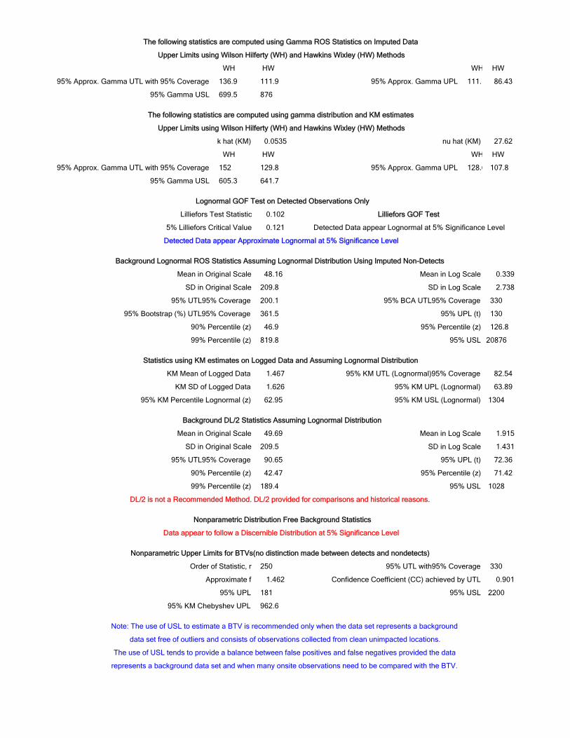
Note: The use of USL to estimate a BTV is recommended only when the data set represents a background
data set free of outliers and consists of observations collected from clean unimpacted locations.
The use of USL tends to provide a balance between false positives and false negatives provided the data
represents a background data set and when many onsite observations need to be compared with the BTV.
95% KM Chebyshev UPL 962.6
Approximate f 1.462 Confidence Coefficient (CC) achieved by UTL 0.901
95% UPL 181 95% USL 2200
Nonparametric Upper Limits for BTVs(no distinction made between detects and nondetects)
Order of Statistic, r 250 95% UTL with95% Coverage 330
DL/2 is not a Recommended Method. DL/2 provided for comparisons and historical reasons.
Nonparametric Distribution Free Background Statistics
Data appear to follow a Discernible Distribution at 5% Significance Level
90% Percentile (z) 42.47 95% Percentile (z) 71.42
99% Percentile (z) 189.4 95% USL 1028
SD in Original Scale 209.5 SD in Log Scale 1.431
95% UTL95% Coverage 90.65 95% UPL (t) 72.36
Background DL/2 Statistics Assuming Lognormal Distribution
Mean in Original Scale 49.69 Mean in Log Scale 1.915
KM SD of Logged Data 1.626 95% KM UPL (Lognormal) 63.89
95% KM Percentile Lognormal (z) 62.95 95% KM USL (Lognormal) 1304
Statistics using KM estimates on Logged Data and Assuming Lognormal Distribution
KM Mean of Logged Data 1.467 95% KM UTL (Lognormal)95% Coverage 82.54
99% Percentile (z) 819.8 95% USL 20876
95% Bootstrap (%) UTL95% Coverage 361.5 95% UPL (t) 130
90% Percentile (z) 46.9 95% Percentile (z) 126.8
SD in Original Scale 209.8 SD in Log Scale 2.738
95% UTL95% Coverage 200.1 95% BCA UTL95% Coverage 330
Background Lognormal ROS Statistics Assuming Lognormal Distribution Using Imputed Non-Detects
Mean in Original Scale 48.16 Mean in Log Scale 0.339
5% Lilliefors Critical Value 0.121 Detected Data appear Lognormal at 5% Significance Level
Detected Data appear Approximate Lognormal at 5% Significance Level
Lognormal GOF Test on Detected Observations Only
Lilliefors Test Statistic 0.102 Lilliefors GOF Test
95% Gamma USL 605.3 641.7
HW
95% Approx. Gamma UTL with 95% Coverage 152 129.8 95% Approx. Gamma UPL 128.6 107.8
WH HW WH
The following statistics are computed using gamma distribution and KM estimates
Upper Limits using Wilson Hilferty (WH) and Hawkins Wixley (HW) Methods
k hat (KM) 0.0535 nu hat (KM) 27.62
86.43
95% Gamma USL 699.5 876
95% Approx. Gamma UTL with 95% Coverage 136.9 111.9 95% Approx. Gamma UPL 111.1
The following statistics are computed using Gamma ROS Statistics on Imputed Data
Upper Limits using Wilson Hilferty (WH) and Hawkins Wixley (HW) Methods
WH HW WH HW

Lognormal GOF Test on Detected Observations Only
Not Enough Data to Perform GOF Test
95% Gamma USL 20 16.14
HW
95% Approx. Gamma UTL with 95% Coverage 8.358 6.895 95% Approx. Gamma UPL 7.5 6.303
WH HW WH
The following statistics are computed using gamma distribution and KM estimates
Upper Limits using Wilson Hilferty (WH) and Hawkins Wixley (HW) Methods
k hat (KM) 0.0413 nu hat (KM) 21.05
MLE Sd (bias corrected) N/A 95% Percentile of Chisquare (2k) N/A
nu hat (MLE) 1599 nu star (bias corrected) N/A
MLE Mean (bias corrected) N/A
k hat (MLE) 399.7 k star (bias corrected MLE) N/A
Theta hat (MLE) 0.5 Theta star (bias corrected MLE) N/A
Gamma GOF Tests on Detected Observations Only
Not Enough Data to Perform GOF Test
Gamma Statistics on Detected Data Only
99% Percentile (z) 61.21 95% USL 80.56
DL/2 is not a recommended method. DL/2 provided for comparisons and historical reasons
95% UTL95% Coverage 52.77 95% UPL (t) 50.17
90% Percentile (z) 44.05 95% Percentile (z) 50.02
DL/2 Substitution Background Statistics Assuming Normal Distribution
Mean 23.02 SD 16.42
90% KM Percentile (z) 25.97 95% KM Percentile (z) 32.32
99% KM Percentile (z) 44.24 95% KM USL 64.85
Mean 3.553 SD 17.49
95% UTL95% Coverage 35.25 95% KM UPL (t) 32.48
Normal GOF Test on Detects Only
Not Enough Data to Perform GOF Test
Kaplan Meier (KM) Background Statistics Assuming Normal Distribution
Critical Values for Background Threshold Values (BTVs)
Tolerance Factor K (For UTL) 1.813 d2max (for USL) 3.505
Warning: Data set has only 2 Detected Values.
This is not enough to compute meaningful or reliable statistics and estimates.
Mean Detected 200 SD Detected 14.14
Mean of Detected Logged Data 5.297 SD of Detected Logged Data 0.0708
Maximum Detect 210 Maximum Non-Detect 56
Variance Detected 200 Percent Non-Detects 99.22%
Number of Distinct Detects 2 Number of Distinct Non-Detects 24
Minimum Detect 190 Minimum Non-Detect 2
Number of Distinct Observations 26
Number of Detects 2 Number of Non-Detects 253
Result (naphthalene)
General Statistics
Total Number of Observations 255 Number of Missing Observations 0

Critical Values for Background Threshold Values (BTVs)
Tolerance Factor K (For UTL) 1.812 d2max (for USL) 3.507
Mean Detected 157.7 SD Detected 104
Mean of Detected Logged Data 4.883 SD of Detected Logged Data 0.596
Maximum Detect 430 Maximum Non-Detect 62
Variance Detected 10809 Percent Non-Detects 93%
Number of Distinct Detects 16 Number of Distinct Non-Detects 24
Minimum Detect 63 Minimum Non-Detect 1
Number of Distinct Observations 40
Number of Detects 18 Number of Non-Detects 239
Result (phenanthrene)
General Statistics
Total Number of Observations 257 Number of Missing Observations 0
Note: The use of USL to estimate a BTV is recommended only when the data set represents a background
data set free of outliers and consists of observations collected from clean unimpacted locations.
The use of USL tends to provide a balance between false positives and false negatives provided the data
represents a background data set and when many onsite observations need to be compared with the BTV.
95% KM Chebyshev UPL 79.93
Approximate f 1.444 Confidence Coefficient (CC) achieved by UTL 0.894
95% UPL 52 95% USL 210
Nonparametric Upper Limits for BTVs(no distinction made between detects and nondetects)
Order of Statistic, r 247 95% UTL with95% Coverage 52
DL/2 is not a Recommended Method. DL/2 provided for comparisons and historical reasons.
Nonparametric Distribution Free Background Statistics
Data do not follow a Discernible Distribution (0.05)
90% Percentile (z) 40.52 95% Percentile (z) 49.06
99% Percentile (z) 70.25 95% USL 130.7
SD in Original Scale 16.42 SD in Log Scale 0.527
95% UTL95% Coverage 53.59 95% UPL (t) 49.3
Background DL/2 Statistics Assuming Lognormal Distribution
Mean in Original Scale 23.02 Mean in Log Scale 3.027
99% Percentile (z) 150.7 95% USL 234.1
95% Bootstrap (%) UTL95% Coverage 125.5 95% UPL (t) 117.2
90% Percentile (z) 102 95% Percentile (z) 116.8
SD in Original Scale 26.84 SD in Log Scale 0.374
95% UTL95% Coverage 124.4 95% BCA UTL95% Coverage 125.5
Background Lognormal ROS Statistics Assuming Lognormal Distribution Using Imputed Non-Detects
Mean in Original Scale 67.81 Mean in Log Scale 4.146

95% Percentile of Chisquare (2k) 1.424 90% Percentile 31.69
95% Percentile 62.71 99% Percentile 156.3
nu hat (MLE) 63.94 nu star (bias corrected) 64.53
MLE Mean (bias corrected) 11.06 MLE Sd (bias corrected) 31.2
k hat (MLE) 0.124 k star (bias corrected MLE) 0.126
Theta hat (MLE) 88.87 Theta star (bias corrected MLE) 88.07
Maximum 430 Median 0.01
SD 48.42 CV 4.379
For gamma distributed detected data, BTVs and UCLs may be computed using gamma distribution on KM estimates
Minimum 0.01 Mean 11.06
Gamma ROS Statistics using Imputed Non-Detects
GROS may not be used when data set has > 50% NDs with many tied observations at multiple DLs
GROS may not be used when kstar of detected data is small such as < 0.1
For such situations, GROS method tends to yield inflated values of UCLs and BTVs
MLE Mean (bias corrected) 157.7
MLE Sd (bias corrected) 99.47 95% Percentile of Chisquare (2k) 11.11
Theta hat (MLE) 53.06 Theta star (bias corrected MLE) 62.73
nu hat (MLE) 107 nu star (bias corrected) 90.51
Gamma Statistics on Detected Data Only
k hat (MLE) 2.973 k star (bias corrected MLE) 2.514
5% K-S Critical Value 0.205 Detected data appear Gamma Distributed at 5% Significance Level
Detected data appear Gamma Distributed at 5% Significance Level
5% A-D Critical Value 0.746 Detected data appear Gamma Distributed at 5% Significance Level
K-S Test Statistic 0.202 Kolmogrov-Smirnoff GOF
Gamma GOF Tests on Detected Observations Only
A-D Test Statistic 0.635 Anderson-Darling GOF Test
99% Percentile (z) 135 95% USL 186.6
DL/2 is not a recommended method. DL/2 provided for comparisons and historical reasons
95% UTL95% Coverage 112.5 95% UPL (t) 105.6
90% Percentile (z) 89.39 95% Percentile (z) 105.2
DL/2 Substitution Background Statistics Assuming Normal Distribution
Mean 33.44 SD 43.65
99% KM Percentile (z) 123.9 95% KM USL 180.7
95% UTL95% Coverage 99.15 95% KM UPL (t) 91.56
90% KM Percentile (z) 73.64 95% KM Percentile (z) 91.11
Kaplan Meier (KM) Background Statistics Assuming Normal Distribution
Mean 11.98 SD 48.11
5% Lilliefors Critical Value 0.209 Data Not Normal at 5% Significance Level
Data Not Normal at 5% Significance Level
5% Shapiro Wilk Critical Value 0.897 Data Not Normal at 5% Significance Level
Lilliefors Test Statistic 0.211 Lilliefors GOF Test
Normal GOF Test on Detects Only
Shapiro Wilk Test Statistic 0.838 Shapiro Wilk GOF Test

Note: The use of USL to estimate a BTV is recommended only when the data set represents a background
data set free of outliers and consists of observations collected from clean unimpacted locations.
The use of USL tends to provide a balance between false positives and false negatives provided the data
represents a background data set and when many onsite observations need to be compared with the BTV.
95% KM Chebyshev UPL 222.1
Approximate f 1.456 Confidence Coefficient (CC) achieved by UTL 0.899
95% UPL 88.3 95% USL 430
Nonparametric Upper Limits for BTVs(no distinction made between detects and nondetects)
Order of Statistic, r 249 95% UTL with95% Coverage 130
DL/2 is not a Recommended Method. DL/2 provided for comparisons and historical reasons.
Nonparametric Distribution Free Background Statistics
Data appear to follow a Discernible Distribution at 5% Significance Level
90% Percentile (z) 62.86 95% Percentile (z) 81.24
99% Percentile (z) 131.4 95% USL 302.5
SD in Original Scale 43.65 SD in Log Scale 0.706
95% UTL95% Coverage 91.4 95% UPL (t) 81.76
Background DL/2 Statistics Assuming Lognormal Distribution
Mean in Original Scale 33.44 Mean in Log Scale 3.236
KM SD of Logged Data 1.256 95% KM UPL (Lognormal) 11.23
95% KM Percentile Lognormal (z) 11.11 95% KM USL (Lognormal) 115.1
Statistics using KM estimates on Logged Data and Assuming Lognormal Distribution
KM Mean of Logged Data 0.342 95% KM UTL (Lognormal)95% Coverage 13.7
99% Percentile (z) 190.2 95% USL 1231
95% Bootstrap (%) UTL95% Coverage 130 95% UPL (t) 65.69
90% Percentile (z) 36.45 95% Percentile (z) 64.74
SD in Original Scale 47.67 SD in Log Scale 1.581
95% UTL95% Coverage 84.3 95% BCA UTL95% Coverage 132
Background Lognormal ROS Statistics Assuming Lognormal Distribution Using Imputed Non-Detects
Mean in Original Scale 18.38 Mean in Log Scale 1.57
5% Lilliefors Critical Value 0.209 Detected Data appear Lognormal at 5% Significance Level
Detected Data appear Lognormal at 5% Significance Level
5% Shapiro Wilk Critical Value 0.897 Detected Data appear Lognormal at 5% Significance Level
Lilliefors Test Statistic 0.18 Lilliefors GOF Test
Lognormal GOF Test on Detected Observations Only
Shapiro Wilk Test Statistic 0.927 Shapiro Wilk GOF Test
95% Gamma USL 138.1 132.6
HW
95% Approx. Gamma UTL with 95% Coverage 35.78 28.9 95% Approx. Gamma UPL 30.4 24.22
WH HW WH
The following statistics are computed using gamma distribution and KM estimates
Upper Limits using Wilson Hilferty (WH) and Hawkins Wixley (HW) Methods
k hat (KM) 0.062 nu hat (KM) 31.85
12.19
95% Gamma USL 135.1 128.1
95% Approx. Gamma UTL with 95% Coverage 24.98 15.87 95% Approx. Gamma UPL 20.0
The following statistics are computed using Gamma ROS Statistics on Imputed Data
Upper Limits using Wilson Hilferty (WH) and Hawkins Wixley (HW) Methods
WH HW WH HW

For gamma distributed detected data, BTVs and UCLs may be computed using gamma distribution on KM estimates
Gamma ROS Statistics using Imputed Non-Detects
GROS may not be used when data set has > 50% NDs with many tied observations at multiple DLs
GROS may not be used when kstar of detected data is small such as < 0.1
For such situations, GROS method tends to yield inflated values of UCLs and BTVs
MLE Mean (bias corrected) 222.7
MLE Sd (bias corrected) 217.3 95% Percentile of Chisquare (2k) 6.185
Theta hat (MLE) 203 Theta star (bias corrected MLE) 212
nu hat (MLE) 122.9 nu star (bias corrected) 117.6
Gamma Statistics on Detected Data Only
k hat (MLE) 1.097 k star (bias corrected MLE) 1.05
5% K-S Critical Value 0.122 Data Not Gamma Distributed at 5% Significance Level
Data Not Gamma Distributed at 5% Significance Level
5% A-D Critical Value 0.777 Data Not Gamma Distributed at 5% Significance Level
K-S Test Statistic 0.191 Kolmogrov-Smirnoff GOF
Gamma GOF Tests on Detected Observations Only
A-D Test Statistic 3.215 Anderson-Darling GOF Test
99% Percentile (z) 414 95% USL 596.3
DL/2 is not a recommended method. DL/2 provided for comparisons and historical reasons
95% UTL95% Coverage 334.9 95% UPL (t) 311.4
90% Percentile (z) 254.6 95% Percentile (z) 310
DL/2 Substitution Background Statistics Assuming Normal Distribution
Mean 59.06 SD 152.6
99% KM Percentile (z) 409.4 95% KM USL 595.4
95% UTL95% Coverage 328.7 95% KM UPL (t) 304.7
90% KM Percentile (z) 246.7 95% KM Percentile (z) 303.3
Kaplan Meier (KM) Background Statistics Assuming Normal Distribution
Mean 47.15 SD 155.7
5% Lilliefors Critical Value 0.118 Data Not Normal at 5% Significance Level
Data Not Normal at 5% Significance Level
5% Shapiro Wilk P Value 1.110E-16 Data Not Normal at 5% Significance Level
Lilliefors Test Statistic 0.289 Lilliefors GOF Test
Normal GOF Test on Detects Only
Shapiro Wilk Test Statistic 0.647 Normal GOF Test on Detected Observations Only
Critical Values for Background Threshold Values (BTVs)
Tolerance Factor K (For UTL) 1.808 d2max (for USL) 3.521
Mean Detected 222.7 SD Detected 281
Mean of Detected Logged Data 4.885 SD of Detected Logged Data 0.949
Maximum Detect 1200 Maximum Non-Detect 41
Variance Detected 78980 Percent Non-Detects 79.18%
Number of Distinct Detects 45 Number of Distinct Non-Detects 18
Minimum Detect 42 Minimum Non-Detect 1
Number of Distinct Observations 63
Number of Detects 56 Number of Non-Detects 213
Result (pyrene)
General Statistics
Total Number of Observations 269 Number of Missing Observations 0

DL/2 is not a Recommended Method. DL/2 provided for comparisons and historical reasons.
Nonparametric Distribution Free Background Statistics
Data appear to follow a Discernible Distribution at 5% Significance Level
90% Percentile (z) 92.36 95% Percentile (z) 135.6
99% Percentile (z) 278.8 95% USL 986.1
SD in Original Scale 152.6 SD in Log Scale 1.058
95% UTL95% Coverage 161.1 95% UPL (t) 136.9
Background DL/2 Statistics Assuming Lognormal Distribution
Mean in Original Scale 59.06 Mean in Log Scale 3.17
KM SD of Logged Data 2.029 95% KM UPL (Lognormal) 79.26
95% KM Percentile Lognormal (z) 77.86 95% KM USL (Lognormal) 3505
Statistics using KM estimates on Logged Data and Assuming Lognormal Distribution
KM Mean of Logged Data 1.017 95% KM UTL (Lognormal)95% Coverage 108.4
99% Percentile (z) 757.2 95% USL 8084
95% Bootstrap (%) UTL95% Coverage 390 95% UPL (t) 199.5
90% Percentile (z) 95.41 95% Percentile (z) 196.1
SD in Original Scale 154.7 SD in Log Scale 1.983
95% UTL95% Coverage 270.8 95% BCA UTL95% Coverage 386
Background Lognormal ROS Statistics Assuming Lognormal Distribution Using Imputed Non-Detects
Mean in Original Scale 52.34 Mean in Log Scale 2.017
5% Lilliefors Critical Value 0.118 Detected Data appear Lognormal at 5% Significance Level
Detected Data appear Approximate Lognormal at 5% Significance Level
Lognormal GOF Test on Detected Observations Only
Lilliefors Test Statistic 0.113 Lilliefors GOF Test
95% Gamma USL 698.1 828.5
HW
95% Approx. Gamma UTL with 95% Coverage 165 149 95% Approx. Gamma UPL 139 122.3
WH HW WH
The following statistics are computed using gamma distribution and KM estimates
Upper Limits using Wilson Hilferty (WH) and Hawkins Wixley (HW) Methods
k hat (KM) 0.0917 nu hat (KM) 49.33
107.5
95% Gamma USL 801.1 1095
95% Approx. Gamma UTL with 95% Coverage 157.1 138.3 95% Approx. Gamma UPL 128.5
The following statistics are computed using Gamma ROS Statistics on Imputed Data
Upper Limits using Wilson Hilferty (WH) and Hawkins Wixley (HW) Methods
WH HW WH HW
95% Percentile of Chisquare (2k) 1.404 90% Percentile 132.4
95% Percentile 263.6 99% Percentile 661.4
nu hat (MLE) 65.81 nu star (bias corrected) 66.41
MLE Mean (bias corrected) 46.37 MLE Sd (bias corrected) 132
k hat (MLE) 0.122 k star (bias corrected MLE) 0.123
Theta hat (MLE) 379.1 Theta star (bias corrected MLE) 375.6
Maximum 1200 Median 0.01
SD 156.2 CV 3.37
Minimum 0.01 Mean 46.37

Note: The use of USL to estimate a BTV is recommended only when the data set represents a background
data set free of outliers and consists of observations collected from clean unimpacted locations.
The use of USL tends to provide a balance between false positives and false negatives provided the data
represents a background data set and when many onsite observations need to be compared with the BTV.
95% KM Chebyshev UPL 727.2
Approximate f 1.526 Confidence Coefficient (CC) achieved by UTL 0.924
95% UPL 235 95% USL 1200
Nonparametric Upper Limits for BTVs(no distinction made between detects and nondetects)
Order of Statistic, r 261 95% UTL with95% Coverage 390

Appendix F
PAH Background Study
Dataset Appropriate for Distribution
(provided as an Excel file)

This page intentionally left blank


