
PFA Development – Definitions and PFA Development – Definitions and PreparationPreparation
0) Generate some events w/G4 in proper format1) Check Sampling Fractions ECAL, HCAL separately
How?Photons, electrons in ECALNeutral hadrons in HCAL (no ECAL int.)Charged Pions in HCAL (don’t forget ECAL mips)
Detector – SDFeb05 Sci HCAL
Photons in ECAL-> sf = 0.012
KL0 in HCAL
-> sf = 0.06

Pions
KL0
KL0
N - ?
Hadron Comparisons
G4 Physics List? – under investigation

PFA Development – Definitions and PFA Development – Definitions and PreparationPreparation
2a) Single Particle Response -> Analytic Perfect PFAExpected values for E resolution?Why not!? -> G4 problem? Go Back To 0)
2b) Analog/Digital Readout!?2a) Calibration
How?With/without threshold cut?Realistic methods?
2b) Choice of threshold cutNecessary?Realistic?

Analytic Perfect PFA – SDFeb05 Detector Model
57 GeV
22 GeV
11 GeV
Photons Hadrons (Pions)
No neutral E!
Photon resolution = 22.5 x .199 = 0.94 GeV
Neutral H resolution = 10.7 x .48 = 1.57 GeV -> PPFA = 19%/E

PFA Development – Definitions and PFA Development – Definitions and PreparationPreparation
3) Perfect PFA with Detector EffectsEqual to 2a)?Better than 30%/√E?
4) Now ready for PFA development
1.31 GeV 1.95 GeV
-> PPFA = 28%/E

PFA Development – Definitions and PFA Development – Definitions and PreparationPreparation
4) Document and archive all of the above for each Detector ModelWeb site for archived plots and detector
documentationAlso needs to include special cuts, etc.
5) Now ready for PFA developmentExamples of PFA use in detector
optimization/evaluation ->

P (e,) = 1 – Ce, e-x/X0
P (h) = 1 – Ch e-l/I
Ce, = (1,7/9)
Ch = 1
1)PFA optimization - beginning of hadron showers separated (longitudinally) from beginning of EM showers . . .
So, in first layers of calorimeter, want P (e,) >> P (h)
-> x/X0 >> l/I
-> I/X0 should be as large as possible
Material I (cm) X0 (cm) I/X0
W 9.59 0.35 27.40
Au 9.74 0.34 28.65
Pt 8.84 0.305 28.98
Pb 17.09 0.56 30.52
U 10.50 0.32 32.81
Calorimeter Absorber Optimization – PFA ApplicationCalorimeter Absorber Optimization – PFA Application
Material I (cm) X0 (cm) I/X0
Fe (SS) 16.76 1.76 9.52
Cu 15.06 1.43 10.53
Dense, Non-magnetic Less Dense, Non-magnetic
. . . Use these for ECAL*
* Note ~X2 difference in I for W/Pb – important for HCAL later

P ()
- P
(h
)
X0X0
P (
inte
ract
ion)
P ()
P (h)
Shower Probabilities in ECAL (25 XShower Probabilities in ECAL (25 X00))
W Absorber
W PbSSCu
P () reaches ~100% while P (h) still <20%-> W,Pb probability differences >> SS,Cu-> better shower separation in dense material

2) Once P (e,) -> 1 and ’s are fully contained (end of
ECAL), want P (h) -> 1 as fast as possible . . .
. . . W performs better than SS and Pb for HCAL
W PbSS
W PbSS
P (
h)
Length (cm) I
dP
(h
)/d I
I 1 1 2 3 2 4 5 3
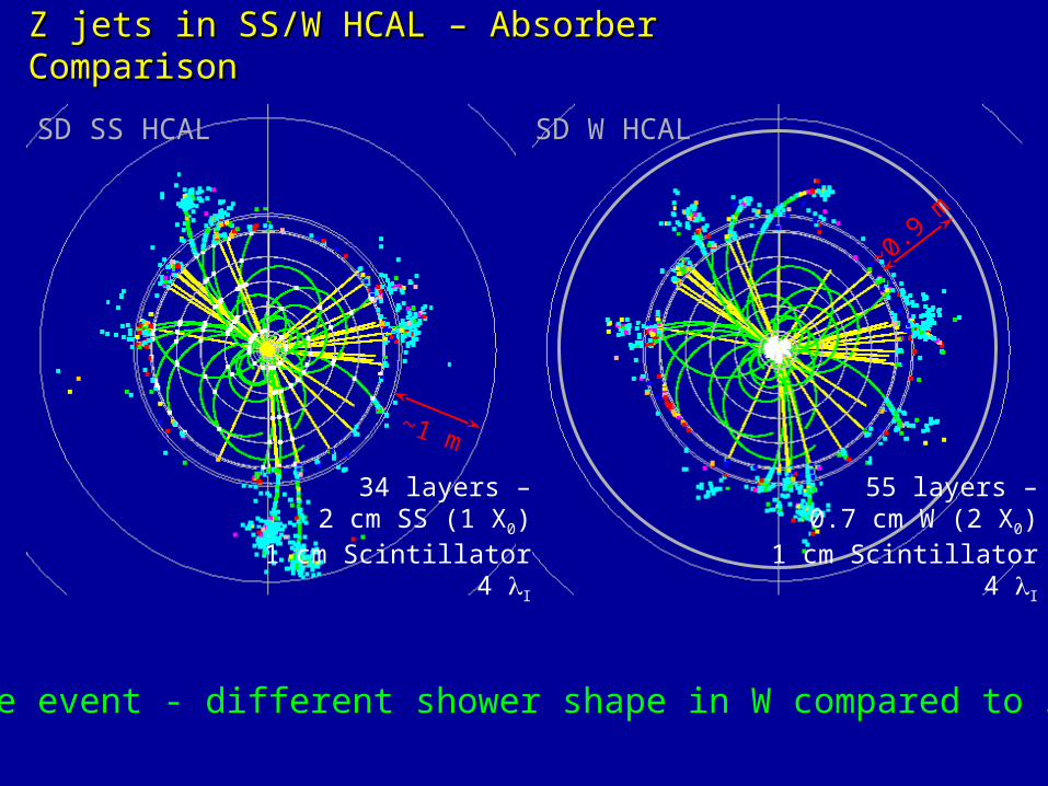
Z jets in SS/W HCAL – Absorber ComparisonZ jets in SS/W HCAL – Absorber Comparison
~1 m
~0.9 m
SD SS HCAL
34 layers –2 cm SS (1 X0)
1 cm Scintillator4 I
SD W HCAL
55 layers –0.7 cm W (2 X0)1 cm Scintillator
4 I
Same event - different shower shape in W compared to SS?
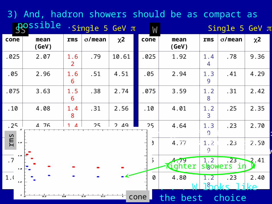
cone
mean (GeV)
rms
/mean
2
.025 1.92 1.44
.78 9.36
.05 2.94 1.39
.41 4.29
.075 3.59 1.28
.31 2.42
.10 4.01 1.23
.25 2.35
.25 4.64 1.30
.23 2.70
.50 4.77 1.29
.23 2.50
.75 4.79 1.28
.23 2.41
1.00 4.80 1.28
.23 2.40
cone
mean (GeV)
rms
/mean
2
.025 2.07 1.62
.79 10.61
.05 2.96 1.66
.51 4.51
.075 3.63 1.56
.38 2.74
.10 4.08 1.48
.31 2.56
.25 4.76 1.44
.25 2.49
.50 4.85 1.43
.25 2.42
.75 4.86 1.42
.25 2.25
1.00 4.87 1.42
.25 2.45
SS W
rms
cone
Energy in fixed cone size :-> means ~same for SS/W-> rms ~10% smaller in W
Tighter showers in W
3) And, hadron showers should be as compact as possible . . .
. . . W looks like the best choice for HCAL
Single 5 GeV Single 5 GeV

SS W
Energy measurement in calorimeter – Analog ECAL, Digital HCAL-> /mean smaller in W HCAL-> same behavior for analog HCAL
4) Energy resolution comparisons for SS, W . . .
E/mean ~ 24% E/mean ~ 20%
Single 5 GeV Pion
W – 2 X0 sampling
SS – 1 X0 sampling

SS W
Single 5 GeV Pion – Number of hits (1/3 mip thresh)Single 5 GeV Pion – Number of hits (1/3 mip thresh)
More hits in W HCAL than in SS-> 30% more hits in the HCAL for W-> better digital resolution for W!
W – 2 X0 sampling
SS – 1 X0 sampling

SS W
Single 5 GeV Pion – Visible Energy in HCALSingle 5 GeV Pion – Visible Energy in HCAL
More visible energy in W HCAL-> better analog resolution in W W – 2 X0 sampling
SS – 1 X0 sampling

SS W
e+e- -> Z (jets) – PFA performance Fitse+e- -> Z (jets) – PFA performance Fits
Better PFA performance with the W HCAL for conical showers . . .however, simple iterative cone reconstructs smaller fraction of events*
True PFA-> SS 33%/E
True PFA-> W 28%/E
W – 2 X0 sampling
SS – 1 X0 sampling

. . . W looks like the best choice for HCAL-> hadron E resolution depends on I, not X0
Single particle, PFA resolution comparison results . . .
0
0.05
0.1
0.15
0.2
0.25
0.3
0.35
1 X0 2 X0
Single pion
PFA
0
0.05
0.1
0.15
0.2
0.25
0.3
0.35
0.07 0.12
Single pion
PFA
E/mean ↓, X0 ↑ ! Coarser X0 sampling gives better
E!?E/mean ↓, I ↓ Finer I sampling gives better
E
E/m
ean
E/m
ean
W – 2 X0 sampling
SS – 1 X0 sampling
W W SSSS

Dense HCALs (W absorber) - 4 I in ~82.5 cm IR -> OR
SDFeb05 SCI HCAL55 layers of 0.7 cm W/0.8 cm Scin.Sampling fraction ~6%
SDFeb05 RPC HCAL55 layers of 0.7 cm W/0.8 cm RPC
1.2 mm gas gapSampling Fraction ~0.0025%!!!
HCAL Readout Optimization – PFA ApplicationHCAL Readout Optimization – PFA Application

First – Calorimeter PerformancesFirst – Calorimeter PerformancesScin. – Analog Readout RPC – Digital Readout
Hard to compete with no visible energy?Not a great start, but lets continue anyway

Track/CAL Cell Association AlgorithmTrack/CAL Cell Association AlgorithmScin. – Analog Readout RPC – Digital Readout
Resolution still better in scintillator, but algorithm reproduces perfect ID in both cases

Neutral Finding AlgorithmNeutral Finding Algorithm
Scin. – Analog Readout RPC – Digital Readout
Once again, very similar performance

PFA ResultsPFA Results
Scin. – Analog Readout RPC – Digital Readout
PFA performance is very similar (with same cuts) but reflects underlying CAL resolution

Confusion – Leftover Hits!Confusion – Leftover Hits!Scin. – Analog Readout RPC – Digital Readout
Better use of hits in RPC? – good since aren’t that many
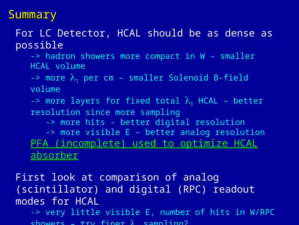
SummarySummary
For LC Detector, HCAL should be as dense as possible
-> hadron showers more compact in W – smaller HCAL volume-> more I per cm – smaller Solenoid B-field volume
-> more layers for fixed total I HCAL – better resolution since more sampling
-> more hits - better digital resolution-> more visible E – better analog resolution
PFA (incomplete) used to optimize HCAL absorber
First look at comparison of analog (scintillator) and digital (RPC) readout modes for HCAL
-> very little visible E, number of hits in W/RPC showers – try finer I sampling?-> compared analog and digital modes with same analysis program
Once again, PFA used to evaluate detector performance

Particle Flow Algorithm – Horse or Cart?
PFA used for :1) Detector Optimization – absorber type/thickness, longitudinal
segmentation and transverse granularity, B-field, tracking volume (radius), etc. -> Detector Model(s)
2) Detector Model evaluation – comparisons, tradeoff evaluations, etc.
-> PFA is the Horse!Physicists still have to do work!


