Physically Based Animation and Rendering of Lightning
Theodore Kim Ming C. LinDepartment of Computer Science
University of North Carolina at Chapel Hill�kim, lin � @cs.unc.edu
http://gamma.cs.unc.edu/LIGHTNING
Abstract
We present a physically-based method for animating andrendering lightning and other electric arcs. For the simula-tion, we present the dielectric breakdown model, an elegantformulation of electrical pattern formation. We then extendthe model to animate a sustained, ‘dancing’ electrical arc,by using a simplified Helmholtz equation for propagatingelectromagnatic waves. For rendering, we use a convolu-tion kernel to produce results competitive with Monte Carloray tracing. Lastly, we present user parameters for manipu-lation of the simulation patterns.
1. Introduction
The forked tendrils of electrical discharge have a longhistory as a dramatic tool in the visual effects industry. Fromthe genesis of the monster in the 1931 movie Frankenstein,to the lightning from the Emperor’s fingers in Return of theJedi, to the demolition of the Coliseum by lightning in lastyear’s The Core, lightning is an ubiquitous effect in sciencefiction and fantasy films.
Despite the popularity of this effect, there has been rela-tively little research into physically-based modeling of thisphenomenon. The existing research is largely empirical, es-sentially generating a random tree-like structure that quali-tatively resembles lightning. The previous work is also lim-ited to brief flashes of lightning, and provides no method foranimating a dancing, sustained stream of electricity. How-ever, modeling the fractal geometry of electrical dischargeand similar patterns has attracted much attention in physics.To our best knowledge, our algorithm is the first rigorous,physically-based modeling of lightning in computer graph-ics. We also believe our approach is accurate enough that itsapplications extend beyond visual effects to more physicallydemanding applications, such as commercial flight simula-tion.
Main Contributions: In this paper, we present a
physically-based algorithm to simulate lightning, andpropose a novel extension for animation of continuous elec-trical streams. The simulation results are then renderedusing an efficient convolution technique. The result-ing image quality rivals that of Monte Carlo ray tracing.Lastly, we present user parameters for intuitive manipu-lation of the simulation. Our approach offers the follow-ing:�
A physically-inspired approach based on the dielectricbreakdown model for electrical discharge;�A novel animation technique for sustained electricalstreams that solves a simplified Helmholtz equation forpropagating electromagnetic waves;�A fast, accurate rendering method that uses a convolu-tion kernel to describe light scattering in participatingmedia;�A parameterization that enables simple artistic controlof the simulation.
Organization: The rest of the paper is organized as fol-lows. A brief survey of related work is presented in Sec. 2.In Sec. 3, we briefly summarize the physics of lightning for-mation. We present the original dielectric breakdown modelas well as our proposed extension in Sec. 4. A efficient ren-dering method is present in Sec. 5. User parameters are pre-sented in Sec. 6, followed by implementation details anddiscussion in Sec. 7. Finally, conclusions and possible di-rections for future work are given in Sec. 8.
2. Previous Work
Reed and Wyvill present a lightning model based on theempirical observation that most lightning branches deviateby an average of 16 degrees from parent branches [14]. Aset of randomly rotated line segments are then generatedwith their angles normally distributed around 16 degrees.In subsequent work, modifications are made to this randomline segment model. Glassner [6] performs a second pass
on the segments to add “tortuosity”, and Kruszewski [9] re-places the normal distribution with a more easily controlledrandomized binary tree.
Notably, Sosorbaram et al. [16] use the dielectric break-down model (DBM) to guide the growth of a random linesegment tree with a local approximation of the potentialfield. But, their approach does not appear to implement fullDBM, as it does not solve the full Laplace equation.
Electric discharges are neither solid, liquid, or gas, butinstead are the fourth phase of matter, plasma. It is a lightsource with no resolvable surface, so traditional renderingtechniques are not directly applicable. To address this prob-lem, Reed and Wyvill [14] describe a ray tracing extensionfor both a lightning bolt and its surrounding glow. Alterna-tively, [16] proposes rendering 3D textures. Dobashi, Ya-mamoto, and Nishita [4] provide the most rigorous treat-ment of the problem by first presenting the associated vol-ume rendering integral, and then presenting an efficient, ap-proximate solution.
In electrical engineering, there are three popular mod-els of electric discharge: gas dynamics [5], electromagnet-ics [1], and distributed circuits [2]. However, none of theseare directly applicable to visual simulation, as they respec-tively approximate the electricity as a cylinder of plasma, athin antenna, and two plates in a circuit.
3. The Physics of Electric Discharge
We classify the physics literature into two categories.The first deals with the physical, experimentally observedproperties of lightning and related electrical patterns. Agood survey of this approach is given by Rakov and Uman[13]. The second is a more qualitative approach that char-acterizes the geometric, fractal properties of electric dis-charge. A good survey of this approach is given by Vicsek[17].
3.1. Physical Properties
Electrical discharge occurs when a large charge differ-ence exists between two objects. For lightning, the caseis usually that the bottom of a cloud has a strong nega-tive charge and the ground possesses a relatively positivecharge. Electrons possess negative charge, the charge differ-ence is then equalized when electrons are transferred fromthe cloud to the ground in the form of lightning. This caseis referred to as ‘downward negative lightning’. While othertypes can exist, downward negative lightning accounts for90 percent of all cloud-to-ground lightning. For illustrativepurposes, we will show here how to simulate this most com-mon type of lightning. But, it should be noted that we canhandle the other types of lightning by trivially manipulat-ing the charge configuration.
Lightning is actually composed of several bolts, or‘strokes’ in rapid succession. The first stroke is referredto as the stepped leader. The subsequent strokes, calleddart leaders, tend to follow the general path of the pre-vious leaders, and do not exhibit as much branching asthe stepped leader. We note that the random line seg-ment approach of previous work in computer graphicsdoes not provide a clear method of simulating dart lead-ers. But, such a method is crucial for simulating sustainedelectric arcs, which are essentially stepped leaders fol-lowed by a large number of dart leaders.
Lightning is initiated in clouds by an event known as theinitial breakdown. During the initial breakdown, the con-ductivity in a small column of air jumps several orders ofmagnitude, effectively transforming the column from an in-sulator (or dielectric) to a conductor. Charge then flows intothe newly conductive air. Another breakdown then occurssomewhere along the perimeter of the newly charged air.This chain of events repeats, forming a thin, tortuous paththrough the air, until the charge reaches the ground.
3.2. Geometric Properties
The physical processes that give rise to the breakdownare still not well understood. However, a great deal ofprogress has been made in characterizing the geometricshape that the breakdown ultimately produces. Electric dis-charge has been observed to have a fractal dimension of ap-proximately 1.7 [11]. Many disparate natural phenomenashare this same fractal dimension, including ice crystals,lichen, and fracture patterns. Collectively, all the patternsthat share these fractal properties are known as Laplaciangrowth phenomena.
There are three techniques for simulating Laplaciangrowth: Diffusion Limited Aggregation [18], the Dielec-tric Breakdown Model [11], and Hastings-Levitov confor-mal mapping [8]. All three produce qualitatively similar re-sults. We elect to use the Dielectric Breakdown Model herebecause it gives the closest correspondence to the phys-ical system being simulated and allows the addition ofnatural, physically intuitive user controls.
4. The Dielectric Breakdown Model
The Dielectric Breakdown Model, or DBM, was first de-scribed by Niemeyer, Pietronero, and Wiesmann [11], and isalso sometimes referred to as the � model. We first presentthe model described in the original paper, and then proposea modification to simulate dart leaders and sustained elec-tric arcs.
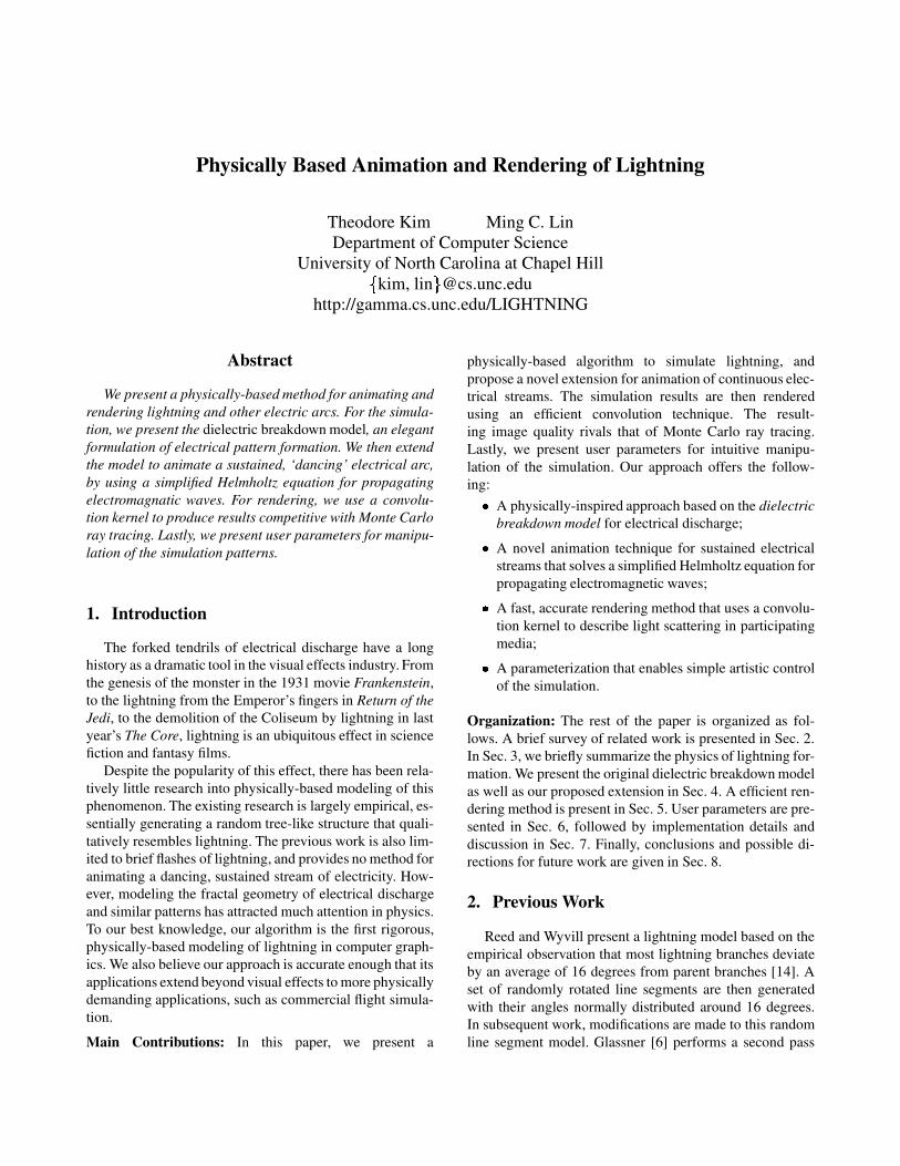
(a) Original configuration (b) Lightning configuration
Figure 1. Different charge configurations forsimulation. Grey: ����� ; Black: ���
4.1. The Laplacian Growth Model
The original charge configuration from [11] is shown inFigure 1(a). Over a 2D grid, the quantity � , the electricalpotential at each point, is tracked. First, a negative charge isplaced at the center by setting ��� � at the center grid cell.Then, a circle of positive charge is constructed around thecenter charge by setting a surrounding circle to ���� . Thepotential at the remaining grid cells are then set by solv-ing the Laplace equation (Eqn. 1) over the grid, with thecenter charge and the surrounding circle treated as bound-ary conditions. The grid boundaries are also set to ����� .��� ������� (1)
The Laplace equation produces a linear system that mustthen be solved. For information on solving the Laplaceequation and the related Poisson equation, the reader is re-ferred to [3]. In our implementation, we solved the sys-tem using conjugate gradient with a diagonal preconditioner[15]. Once the Laplace equation has been solved, we con-struct a list of all the grid cells that are adjacent to a nega-tive charge ( ���� ). One of these grid cells is then randomlychosen as a growth site (i.e. the site of the next breakdown).The chosen cell is set to ����� and is treated as part of theboundary condition in subsequent iterations. The probabil-ity of a grid cell being chosen is weighted according to itspotential. The weight function is given in Eqn 2.
��� � � � ����� �!"$#&% � � " � � (2)
where ' is a cell in the list of adjacent cells, and ( is the totalnumber of cells in the list. The � term is a user parameterthat will be discussed in section 6.
Subsequent iterations proceed by solving the Laplaceequation again over the 2D domain, and again selecting a
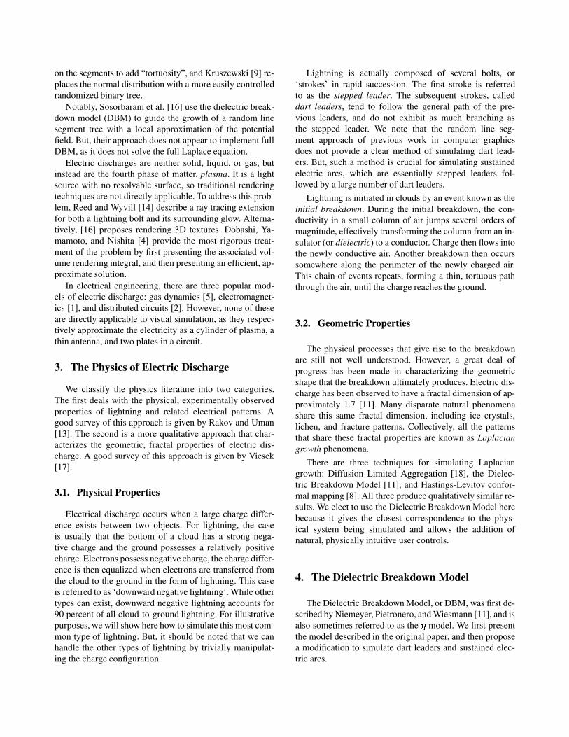
(a) Original configuration (b) )+*�,
(c) )+*- (d) )+*.Figure 2. Simulation results from differentcharge configurations. 2(a) is result of con-figuration from Figure 1(a). 2(b) - 2(d) are con-figurations from 1(b) with various � .
growth site according to Eqn 2. The iterations are repeateduntil the user obtains the desired results. The technique gen-eralizes trivially to three dimensions by simply solving the3D Laplace equation.
The classic configuration produces a radial discharge, asshown in Figure 2(a). In order to produce lightning-like pat-terns, we instead use the initial configuration shown in Fig-ure 1(b). We start with a small amount of negative chargeat the top of the 3D domain, representing an initial branchof lightning. The bottom edge of the domain represents theground, and is thus set to positive charge. The remaininggrid edges are again set to ����� . The results of running thesimulation on this initial configuration with different � areshown in Figures 2(b) - 2(d).
4.2. A Poisson Growth Model
Once we have formed an initial stepped leader, we wouldlike to have a method for generating subsequent dart leadersthat follow the same general path. Since the path changesslightly with each successive dart leader, a large number of
dart leaders will produce the ‘dancing’ effect present in asustained electric arc.
We hypothesize that the reason that a dart leader followsthe same general path as a stepped leader is because thereexists residual positive charge along the old leader chan-nel that attracts the new dart leader. In order to simulate thisbehavior, we need a method of introducing residual chargeinto the simulation.
While DBM can simulate many different kinds of natu-ral phenomena, we observe that for the case of electricity,the Laplace equation can be viewed as a special case of theHelmholtz equation for propagating electromagnetic waves(Eqn 3). / � �1032�4 576 �98 ���;:=<?>A@ (3)
where 4 is angular velocity,5
is the speed of light, and @is charge density. The Helmholtz equation is derived di-rectly from the Maxwell equations for electricity and mag-netism, so it provides a clean connection between fractalgrowth and classical physics. The Laplace equation can beviewed as the case where the charge density is equal to zeroand the relativistic BDC EGF � term is ignored. As lightning boltshave a linear velocity that already approaches the speed oflight, the angular component should be negligible. So, if wecontinue to ignore the relativistic term but re-introduce thecharge density term, the electromagnetic Poisson equationis obtained:
� � ���;:=<?>A@H� (4)
If we now solve this equation in place of the Laplace equa-tion, we can produce the desired dart leader behavior. Thevalue of @ is determined by a second grid of values in spacethat is initially set to zero. This essentially reduces Eqn. 4 tothe Laplace equation for the initial iteration. After we gen-erate our first bolt, we deposit charge along the leader chan-nel by setting @ in the cells along the channel to a positivevalue. When generating subsequent bolts, the new @ valueswill automatically attract the new bolt to the old path. Af-ter each new bolt is generated, we clear the previous @ fieldand repopulate it with charges along the new leader chan-nel.
Fortunately, because the Poisson and Laplace equationsare very similar, the only implementation overhead requiredfor our modified model is a minor change to the residual cal-culation in the conjugate gradient solver. It is worth notingthat a similar model has been proposed in the physics liter-ature [12] which also accounts for inhomogeneous dielec-tric permittivities. Our model was developed independently.For efficient visual rendering, we choose to ignore inhomo-geneity and treat air as a homogeneous media.
5. Rendering
For the rendering of electricity, we borrow the method ofNarasimhan and Nayar [10]. In the paper, analytical mod-els are obtained that reduce the rendering of certain typesof participating media to a 2D convolution. The results arecompetitive with expensive Monte Carlo techniques suchas photon mapping, but run in seconds instead of hours. Wewill first summarize the pertinent formulae from [10], thendescribe how we use it to generate a convolution kernel, andfinally show how we render electricity.
5.1. Atmospheric Point Spread Function
The convolution kernel produced by the method of [10]is called an Atmospheric Point Spread Function, hereon re-ferred to as an APSF. The APSF is a series expansion ofthe Henyey-Greenstein phase function, a popular functionfor describing the scattering of light in participating media.The basis functions used are Legendre polynomials, whoseseries form are shown in Eqn. 5.
I � �KJ � � �$�ML '&:N �PO J O I �RQ % �RJ � : �$� 'S:T �PO I �RQ � �KJ �$�'(5)
In order the evaluate the series, the following base cases arealso necessary:
I1U �KJ � �V , I % �KJ � � J . The full APSF,W �RXZY\[ � , is then given in Eqn. 6.
W �KXZY$[ � �^]_` # U �Ra ` �RX � 0 a `+b % �KX � I ` �K[ �$� (6)
where
a ` �KX � � c QGdfePgSQihjekg (7)l ` � m 0 (8)n ` � L m 0 m � Z:po ` Q % � � (9)
Again a base case is necessary: a U �KX � �q� . The variableo is the scattering parameter from the Henyey-Greensteinphase function. Increasing o from 0 to 1 increases the den-sity of the medium, and can be thought of as transitioningthe weather from clear skies to rain. The optical thickness,X , is equal to rts , where r is the radial distance from theviewer, and s is the extinction coefficient of air. Finally [ isthe cosine of the radial direction u from the source.
5.2. Generating a Convolution Kernel
The APSF is a three dimensional function that describeshow much light is reaching any point in space around apoint light source. If we can determine how a single point
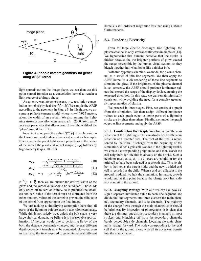
Figure 3. Pinhole camera geometry for gener-ating APSF kernel
light spreads out on the image plane, we can then use thispoint spread function as a convolution kernel to render alight source of arbitrary shape.
Assume we want to generate an (�vw( resolution convo-lution kernel of physical size xyvzx . We sample the APSFaccording to the geometry in Figure 3. In this figure, we as-sume a pinhole camera model where {��|��� � Lj} meters,about the width of an eyeball. We also assume the light-ning stroke is two kilometers away: ~�� L �j�?� . We treat ras a user parameter that allows control over the width of the‘glow’ around the stroke.
In order to compute the valueW �KX�Y\[ � at each point on
the kernel, we need to determine a value [ at each sample.If we assume the point light source projects onto the centerof the kernel, the [ value at kernel sample �KJ&Y\� � follows bytrigonometry (Eqns. 10 - 12).
�f�?� � ��� � � Q+� ���$�G�! 0 � � Q+� �j�$���! (10)4 ��� � ��� �\� Q �f� Qi� ���� � � � b � �\�A� b � ���� � �A�� � b � ���� � (11)
[ �?� � ��>:������ Q % �� ��� � :¡ \¢£� Q % � Q C �¤� ��(12)
If� �¤� �� ¥
��, then we are outside the desired width of the
glow, and the kernel value should be set to zero. The APSFonly drops off to zero at infinity, so in practice, the small-est non-zero value of the kernel must be subtracted from theother non-zero values of the kernel to prevent the silhouetteof the kernel from appearing in the final image.
We are making a simplifying assumption here that allparts of the lightning bolt are exactly two kilometers away.While this is not strictly true, unless the bolt spans a verylarge physical domain, we believe it is a reasonable approx-imation. If the user would like to perform a fly-by of thebolt, the distance constantly changes, and several differentdepth-dependent kernels must be computed. However, evenin this case, the time required to generate several different
kernels is still orders of magnitude less than using a MonteCarlo renderer.
5.3. Rendering Electricity
Even for large electric discharges like lightning, theplasma channel is only several centimeters in diameter [13].We hypothesize that humans perceive that the stroke isthicker because the the brighter portions of glow exceedthe range perceptible by the human visual system, so theybleach together into what looks like a thicker bolt.
With this hypothesis in mind, we model the plasma chan-nel as a series of thin line segments. We then apply theAPSF kernel to a 2D rendering of these line segments tosimulate the glow. If the brightness of the plasma channelis set correctly, the APSF should produce luminance val-ues that exceed the range of the display device, creating theexpected thick bolt. In this way, we can remain physicallyconsistent while avoiding the need for a complex geomet-ric representation of plasma.
We proceed in three stages. First, we construct a graphfrom the simulation. We then assign different luminancevalues to each graph edge, as some parts of a lightningstroke are brighter than others. Finally, we render the graphedges as line segments and apply the APSF.
5.3.1. Constructing the Graph We observe that the con-struction of the lightning stroke can also be seen as the con-struction of a directed tree. The root of the tree is repre-sented by the initial discharge from the beginning of thesimulation. When a grid cell is added to the lightning stroke,we create a corresponding graph node, and then search thecell neighbors for one that is already on the stroke. Such aneighbor must exist, as it is a necessary condition for thegrid cell to have been selected as a growth site. This neigh-bor is then set as the parent node, and the newly added gridcell is recorded as the child. When a grid cell adjacent to theground is added, we halt the simulation. In nature, growthwould end at this point because the charge now has a di-rect conduit to the ground.
5.3.2. Assigning Wattage With our tree, we can now as-sign a separate luminance value to each line segment. Wedivide the line segments into three classes: the main chan-nel, secondary channels, and side channels. The majorityof the charge flows through the main channel, so it shouldbe brightest. By inspection of photographs, it is clear thatthere are dimmer but distinct secondary channels in moststrokes, and branching off from the secondary channels,barely perceptible side channels. Locating the main chan-nel is straightforward. The node corresponding to the gridcell that hit the ground, along with all its ancestors, consti-tute the main channel.
Locating the secondary and side channels is more in-volved. Every node adjacent to the main channel that is noton the main channel forms the root to a new tree. Withineach such tree, the charge selects a preferred path that be-comes the bright secondary channel. There is a poverty oftheories on how this path is selected; perhaps the path thathad the largest potential differences during the breakdownprocess is selected. For aesthetic effect, we set the pathwith the greatest number of nodes as the secondary chan-nel. Off of this longest secondary channel, we also add other‘long’ paths according to a user-defined cutoff. This tech-nique maximizes the length of the dramatic, snaking ten-drils that surround the central channel. All the remainingedges are now considered to be side channels.
We must now assign a wattage to each edge. While thereexists some data on the wattage of the main channel (Be-tween j� ¦7v§9�j¨ Watts / m and ¦G� ©7v§9�jª Watts / m accordingto [13]), we have been unable to find data on the wattage ofsecondary or side channels. We have attempted to estimatethe wattages by deconvolving photographs of lightning, butthis method requires a high dynamic range image of light-ning that can resolve the bleached portion of the stroke, aswell as the APSF values corresponding to the scene. We in-stead used heuristic values that brought us into close quali-tative agreement with photographs.
We rendered the line segments and convolved them withthe APSF settings given in Table 1. The resulting image wasthen composited into a raytraced rendering of the remain-ing scene objects. We do not set the main channel to thewattage given by [13], because in the absence of tone map-ping, this step would bleach the entire scene. The applica-tion of tone mapping to lightning rendering is discussed inour future work.
Figure n M q m T R4, 5, 7 256 1.0 0.99 200 1.001 200
6 64 1.0 0.9 200 1.1 100
Table 1. APSF settings used: m correspondsto the number of terms used in the Legendreseries.
6. User Controls
Our modified DBM permits user control through four pa-rameters: an � variable to control the ‘branchiness’ of thestream, a charge density field @ to control the path of thestream, a boundary condition to repel the stream, and anoverall charge configuration to control where the stroke be-gins and ends.
The effect of the � variable in Eqn. 2 can be seen in Fig-ure 2(b) - 2(d). At ���« , dense branching is observed. As
� increases, the density of the branching decreases. Hast-ings observes that at ���¬< , the stream transitions into anon-fractal, one-dimensional curve [7]. So, the domain ofthe � parameter is effectively in the range of � Y < � . A phys-ical interpretation of � is not entirely clear, it can perhapsbe viewed as the amount of resistance that the air offers tothe process of dielectric breakdown.
As @ is a 2D field representing the image plane, the usercan ‘paint’ into it any desired charge distribution. The light-ning stroke will then be attracted to this painted path as de-scribed in Section 4.2.
In addition to attracting the electric arc, the user maywant to repel the arc from certain regions. For instance,there may be an obstacle in the scene that the user doesnot want the arc to intersect. This effect can be achievedby setting the interior of the obstacle to ��®� . This setsthe charge of the object to the same charge as the arc, caus-ing the obstacle to repel the arc. However, we must thenbe careful in our implementation not to add grid cells adja-cent to the obstacle to the list of candidate growth sites inEqn. 2.
Finally, we have only shown two charge configurations:the circle in Figure 1(a), and the lightning configuration inFigure 1(b). However, arbitrary charge configurations alsoproduce electric arcs. The arc can begin from any arbitrarilyshaped negative region, and terminate at a positive object.In this way, it is possible to construct an arc between anytwo objects in an arbitrary scene.
7. Implementation and Results
We have implemented our algorithm in C++. We ran sim-ulations for several scenes on a 2.66 GHz Xeon processor.Unless otherwise noted, all simulations were performed ona } L v } L grid with ��¯ and @�� % U°U°U±°² along the mainchannel. The renderings were performed in POV-Ray, andthen convolved and composited using ImageMagick. Al-though we set �³�´ , the final results tend to resemble thosewhere ��� L and ¦ . This is because the majority of thegrowth sites are treated as side channels, and are thus verydim. However, we found that in order to obtain long, dra-matic, secondary channels, setting �µ�� was necessary.
Note that when implementing Eqn. 5, recursively eval-uating the series is an exponential time operation. How-ever, evaluating from the bottom up (i.e. in the orderIkU �RJ � Y I % �KJ � Y I � �KJ � ...) is a dynamic programming solu-tion that can be done in linear time. Using this method ismore efficient. Also, as the convolution kernel in subsec-tion 5.2 is separable, it can be performed quickly with two(�vp filters instead of one (pv�( filter.
In Figure 4, we demonstrate how the user can repel thebolt from arbitrary objects. The lightning must start fromthe top of the Cornell Box and find a path to the floor,
while avoiding the two beams in the center. In Figure 5, wedemonstrate how the user can attract the bolt to an arbitraryobject. The magenta electrode in the center is set to a nega-tive charge, and blue ball is set to a positive charge. As theblue ball moves, the electric arc follows. In Figure 7, we an-imate a dancing electric arc between two electrodes. In Fig-ure 6, we validate our results by comparing our renderingswith a photograph. The scene was simulated on a L?}?¶¸· grid.
8. Conclusion and Future Work
We have presented a physically based algorithm for thesimulation, animation, and rendering of sustained electricarcs. We believe that our approach is the most rigorous,physically consistent method available up to date. However,there are several areas for refinement.
Primarily, the simulation can be very slow. For large 2Dand 3D grids, the computation time can take hours. But, itis unclear if other Laplacian growth methods, such as DLAor Hastings-Levitov conformal mapping, can give superiorperformance while preserving the same level of control.
While our rendering method is physically consistent, itwould be more realistic to use some sort of tone mappingoperator to bring the luminance values back into the rangeof the display device. No operator was used here becausewe were unsure which would be appropriate. In the tonemapping literature, a ‘bright’ object is usually daylight or alightbulb, so it is unclear if some of these methods wouldbreak down in the presence of luminance values many or-ders of magnitude brighter.
While the use of the convolution kernel generates im-pressive results, there are still some unresolved issues. It as-sumes the scattering medium is homogeneous, so it doesnot explicitly handle the effects of either internal obstaclesor clouds. A scene requiring a volume caustic still needsa Monte Carlo renderer. The approach described in [4] ap-pears to be the best solution for a scene containing clouds.While an analytical solution may also be possible for thesecases, one has not yet been found.
Finally, we have only presented one type of Lapla-cian growth: electric arcs. Laplacian growth encompassesmany disparate phenomena, including ice formation, ma-terial fracture, lichen growth, tree growth, liquid surfacetension, vasculature patterns, river formation, and even ur-ban sprawl. Modeling of Laplacian growth is well worthexploring for visual simulation of natural phenomena.
Acknowledgements
The authors would like to thank Srinivasa Narasimhanfor his help with the APSF, and the anonymous reviewersfor their help in improving this manuscript. The photo inFigure 6 is c
¹Warren Faidley/Weatherstock.com and is used
with permission. This work was supported in part by ArmyResearch Office, Intel Corporation, National Science Foun-dation, and Office of Naval Research.
References
[1] Y. Baba and M. Ishii. Numerical electromagnetic field anal-ysis of lightning current in tall structures. IEEE Trans. Pow.Rel., 16:324–328, 2001.
[2] C. Baum and L. Baker. Analytic return-stroke transmission-line model. Electromagnetics, 7:205–228, 1987.
[3] J. Demmel. Applied Numerical Linear Algebra. SIAM,1997.
[4] Y. Dobashi, T. Yamamoto, and T. Nishita. Efficient render-ing of lightning tacking into account scattering effects dueto clouds and atmospheric particles. Proc. of Pacific Graph-ics, 2001.
[5] E. Dubovoy, M. Mikhailov, A. Ogonkov, and V. Pryazhin-sky. Measurement and numerical modeling of radio sound-ing reflection from a lightning channel. J. Geophys. Res.,100:1497–1502, 1995.
[6] A. Glassner. The digital ceraunoscope: Synthetic thunderand lightning. Technical Report MSR-TR-99-17, MicrosoftResearch, 1999.
[7] M. Hastings. Fractal to nonfractal phase transition in the di-electric breakdown model. Physical Review Letters, 87(17),2001.
[8] M. Hastings and L. Levitov. Laplacian growth as one-dimensional turbulence. Physica D, 116:244–252, 1998.
[9] P. Kruszewski. A probabilistic technique for the syntheticimagery of lightning. Computers and Graphics, 1999.
[10] S. Narasimhan and S. Nayar. Shedding light on the weather.Proceedings of IEEE CVPR, 2003.
[11] L. Niemeyer, L. Pietronero, and H. J. Wiesmann. Fractal di-mension of dielectric breakdown. Physical Review Letters,52:1033–1036, 1984.
[12] M. Noskov, V. Kukhta, and V. Lopatin. Simulation of theelectrical discharge development in inhomogeneous insula-tors. Journal of Physics D, 28:1187–1194, 1995.
[13] V. Rakov and M. Uman. Lightning: Physics and Effects.Cambridge University Press, 2003.
[14] T. Reed and B. Wyvill. Visual simulation of lightning. Proc.of SIGGRAPH, 1994.
[15] J. R. Shewchuk. An introduction to the conjugate gradi-ent method without the agonizing pain. Technical report,Carnegie Mellon University, 1994.
[16] B. Sosorbaram, T. Fujimoto, K. Muraoka, and N. Chiba.Visual simulation of lightning taking into account cloudgrowth. Computer Graphics International, 2001.
[17] T. Vicsek. Fractal Growth Phenomena. World Scientific,1992.
[18] T. Witten and L. Sander. Diffusion-limited aggregation,a kinetic critical phenomenon. Physical Review Letters,47(19):pp. 1400–1403, 1981.
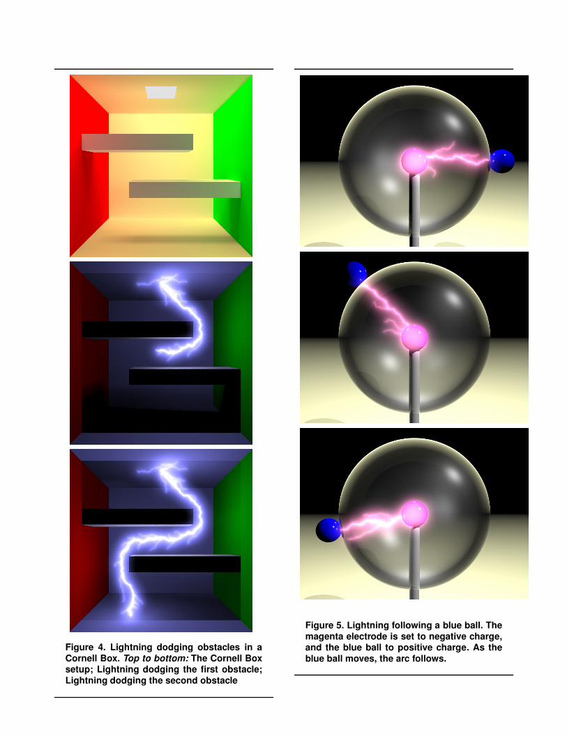
Figure 4. Lightning dodging obstacles in aCornell Box. Top to bottom: The Cornell Boxsetup; Lightning dodging the first obstacle;Lightning dodging the second obstacle
Figure 5. Lightning following a blue ball. Themagenta electrode is set to negative charge,and the blue ball to positive charge. As theblue ball moves, the arc follows.
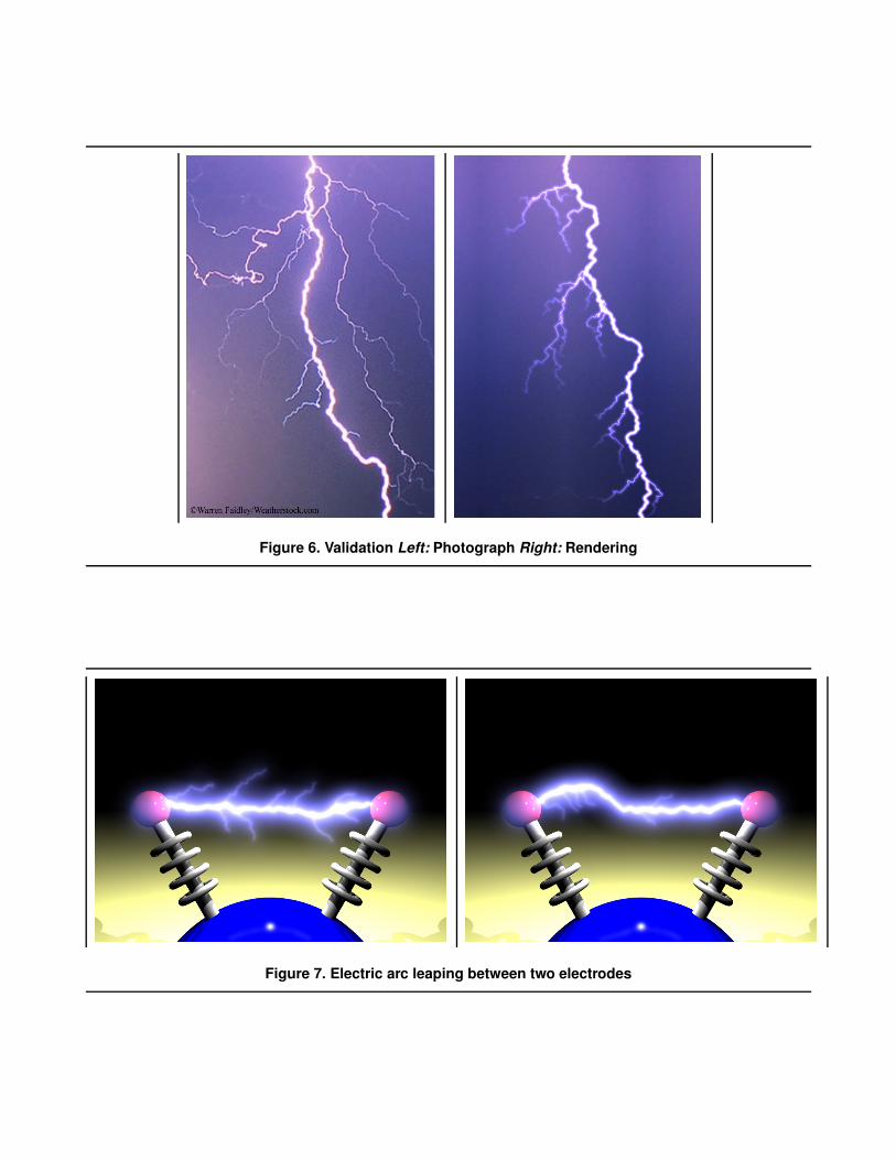
Figure 6. Validation Left: Photograph Right: Rendering
Figure 7. Electric arc leaping between two electrodes


