
Political-economy of healthcare provision in India: Analysing the
entire healthcare distribution
Subham Kailthya ∗& Uma Kambhampati †
Abstract
The public provision of healthcare is common in democracies. Conventional approaches
to examine the link between political economy variables and healthcare provision focus on
the average effect. However, the relationship at the extremes – when healthcare provision is
extremely low or when it is remarkably high – may be quite different. This distinction is
important from a policy perspective because it can affect many lives. We use cross-sectional
data from the Indian District Level Household and Facility Survey for the year 2007-08 to
examine the impact of three main political economy variables – political competition, voter
turnout and effective number of parties – on different measures of healthcare provision and
at different points along the conditional healthcare distribution using quantile regressions.
In most instances, we find that it is political stability rather than political competition
that is associated with improved healthcare service delivery in India. The effect of turnout is
mixed i.e. while its impact is positive for some healthcare measures, it is negative for others.
For effective number of parties, we find a positive association in a majority of the cases which
would suggest that a broader distribution of political power has had a favourable impact on
healthcare service delivery. Importantly, these effects are heterogeneous along the conditional
healthcare distribution. Our results are robust to heteroscedasticity and misspecification
bias. We use several robustness checks to ensure the validity of our results.
Keywords: Political economics; Local government spending; healthcare; quantile regres-
sions; India
JEL codes: D78; H40; H75; C31; I18
1 Introduction
The provision of healthcare – who funds it, and how – are issues occupying governments in
both the developed and developing countries. While the mode of healthcare service delivery
might vary across countries, some form of government intervention in healthcare is almost
universal (Glied et al. 2012). Because of the widespread government intervention, there is a
growing literature that examines the political economy of publicly provided healthcare. The
standard approach to examine this relationship focuses on point estimates at the conditional
∗Corresponding author: Postdoctoral Research Assistant, Department of Economics, University of Reading,Whiteknights. Email address: [email protected]†Professor, Department of Economics, University of Reading.
1

mean obtained by estimators like the least squares. The picture that emerges from averaging
out over the whole healthcare distribution is however incomplete since the relationship between
local political economic variables and healthcare provision for regions lying at one end of the
healthcare distribution, say the top quantile, may indeed be quite different from those lying at
the bottom quantile. In this paper, we argue for adopting a more comprehensive approach to
understand the link between political economics and public healthcare provision by examining
the association at different points along the entire conditional healthcare distribution.
The support for government intervention in healthcare is often justified due to equity concerns –
as the poor may not be able to afford high-cost healthcare; large positive externality benefits
such as from immunizations which significantly limit the spread of infectious diseases; due
to large information gaps that hinder the development of insurance markets; and from the
consideration that healthcare infrastructure is a public good (Glied et al. 2012) These conditions
that lead to market failures become even more acute in developing countries where inadequate
health insurance coverage and high out-of-pocket expenses relating to healthcare means that an
episode of sickness in many instances translate into a debilitating shock to human well-being, not
only from lost productivity or physical impairment but also from the stress and strains caused
by indebtedness (van Doorslaer et al. 2006) Because healthcare provision can affect so many
lives, it is important to understand the link between political economics and publicly provided
healthcare.
When groups within the electorate differ in their preferences for publicly provided healthcare,
the relationship between political economic factors and publicly provided healthcare becomes
hard to predict ex-ante. On the one hand, it is reasonable to argue that the top priority of
voters in regions underserved by public healthcare would be to increase its provision. On the
other hand, if healthcare supply creates its own demand, it is equally likely that further calls for
improvements in healthcare would come from voters who already benefit from good healthcare.
These conditions imply that the spread of the conditonal healthcare distribution is not likely to
be the same across these groups and the association between political economics and healthcare
provision is likely to vary along the conditional healthcare distribution.
From a policy perspective, in explaining regional disparities in healthcare provision, it is
interesting to examine not only how the explanatory variables affect the dependent variable
on average, but also how it affects the extremes of the conditional distribution of healthcare
provision. In this paper, we concentrate on examining the association between different measures
of healthcare provision and three main political economy variables – political participation of
citizens, electoral competition and effective number of parties (ENP) – in the context of India.
For example, does an increase in political participation have the same effect on healthcare
provision for regions which are in the top quantile of healthcare provision as they do for regions
that are in the bottom quantile? And what would be its magnitude and direction? Similarly,
does the effect of electoral competition and ENP vary along the conditional distribution of
healthcare provision? Given the hierarchical structure of the Indian public healthcare system,
where different tiers specialize in offering different kinds of services, we investigate which aspects
of healthcare provision are more sensitive to changes in political market characteristics.
The arguments that motivate an approach that looks beyond the mean become even more salient
when the distribution of healthcare provision is skewed: for instance, while on average 41% of
2

villages within a district have access to a health subcentre in our sample, it is 21% at the 10th
percentile, and 68% at the 90th percentile. Given such wide disparities in healthcare provision,
do regions that lie at the lower end of the (conditional) healthcare distribution, say the bottom
quantile, exhibit a different relationship with political economy variables than regions located
at the top-most quantile? A quick visualization might aid in understanding the heterogenous
relationship. In Figure 1 we divide the unconditional distributions of two variables – access to
health subcentres and the presence of female doctors at primary health centres – into quartiles
ranging from poor access (low presence of female doctors) to good access (high presence of female
doctors). While those in the first quartile are the poorest fourth in terms of access to health
subcentres (presence of female doctors), those in the fourth quartile are better-off than the lower
three-fourths of the sample. Once we arrange them in this way, we plot the corresponding mean
values for each of the three main political economic variables that we focus in this study – vote
margin (or electoral competition, Panel (a)), turnout (Panel (b)) and ENP (Panel (c))– on the
vertical axis. As we can observe from the figure, the unconditional relationship is heterogeneous:
places with better access to health subcentres (high presence of female doctors) are associated,
on average, with lower political competition (or a higher margin of victory) and lower ENP, but
higher turnout in comparson to places with poorer access to health subcentres (low presence of
female doctors).
.14
.15
.16
.17
Vote
marg
in, m
ean
Poor 2 3 GoodQuartiles
HSC−Access PHC−FMO
(a) Vote margin
.56
.58
.6.6
2.6
4.6
6T
urn
out, m
ean
Poor 2 3 GoodQuartiles
HSC−Access PHC−FMO
(b) Turnout
2.4
2.5
2.6
2.7
2.8
EN
P, m
ean
Poor 2 3 GoodQuartiles
HSC−Access PHC−FMO
(c) ENP
Figure 1: Relationship between political economic variables and healthcare provision at differentquartiles of the unconditional distribution. HSC-Access = % of villages in a district that haveaccess to HSC within the village, PHC-FMO = % of PHCs in a district where a female doctor ispresent.
When distributions are heterogenous, like the one we observe in Figure 1, regressions focusing on
the mean might under or overestimate effects or even fail to identify effects (Cade and Noon 2003).
One way to avoid this problem is to use quantile regressions (Koenker and Bassett 1978, Koenker
and Hallock 2001, Koenker 2005) to study the effect of our covariates on different aspects of
healthcare provision. The advantage of using a quantile regression is that it allows us to quantify
the effect of our covariates at different points along the conditional healthcare distribution
instead of focusing exclusively on the average. Using this method will therefore provide a more
nuanced picture of the association between political economic factors and healthcare provision.
In this paper, we ask three specific questions: (a) is political stability more salient than political
competition in improving healthcare provision?; (b) is voter turnout positively correlated with
3

healthcare provision?; and (c) does a broader distribution of political power (measured by ENP)
improve healthcare provision?
To analyse these questions, we use district-level cross-esectional data from the third round of
the Indian District Level Household and Facility Survey (DLHS-3) conducted in 2007-08.1 For
the purpose of this study, we focus on 15 major Indian states.2 We combine this with electoral
and socio-economic data from multiple sources which we discuss later on. India provides a
rich set of variations to study these issues. It is a large and mature democracy that has had
relatively fair elections at regular intervals for almost seventy years. It is geographically vast
with the different administrative divisions bound together by a common legal and administrative
framework. Once we control for confounding factors, these variations in our dataset helps us
to identify the political economic correlates of publicly provided healthcare at different points
along the conditional healthcare distributions.
We find that high political competition is largely associated with low healthcare provision which is
not surprising once the institutional context is considered. The effect of turnout is mixed, whereas
ENP is positively associated with healthcare provision in a majority of the cases. Importantly,
the impact of political economy variables on healthcare provision is heterogeneous. This holds
true across multiple measures of healthcare provision and across the different components of the
hierarchical public healthcare system in India.
The rest of the paper is organized as follows: Section 2 provides institutional background and
describes the organizational structure of public healthcare service delivery in India. Section 3
summarizes the related literature. Section 4 outlines the main hypotheses we intend to test.
Section 5 describes the methodology. Section 6 introduces the data set, discusses the selection
of variables and specifies the econometric model to test our hypotheses. Section 7 discusses
regression results. We conduct several robustness checks which we present in Section 8. Section
9 concludes.
2 Background
2.1 Institutional background
The Indian Constitution, in its Directive Principles of State Policy mentions that one of the
duties of the States is to improve public health, nutrition, and the standard of living of the
people. Unlike fundamental rights, the directive principles are not enforceable. However, they
are an integral part of the Constitution and serve as guiding principles for the States in policy
making.
India is a federation of States. The Indian Constitution, in its Seventh Schedule outlines the
legislative and financial responsibilities of the Centre and the States in the Union list, the State
list and the Concurrent list. While the Union list contains matters of national interest; those
within the domain of the States are in the State list; whereas, the Concurrent List contains items
1Districts are administrative units lower in hierarchy than the States and play an instrumental role indecision-making with regard to socio-economic development.
2The states covered in this study are: Andhra Pradesh, Assam, Bihar, Gujarat, Haryana, Karnataka, Kerala,Madhya Pradesh, Maharashtra, Orissa, Punjab, Rajasthan, Tamil Nadu, Uttar Pradesh and West Bengal.
4
that can be legislated upon by both the Centre and the States. With regard to healthcare, public
health and sanitation, hospitals and dispensaries are the State’s responsibility; whereas medical
education, medical professionals, population and family control are under the joint responsibility
of the Centre and the States.
The 73rd Amendment Act (1992) devolved powers and responsibilities to the grassroots by
creating a third tier of local governance – the Panchayats (in rural areas) and municipalities
(in urban areas). Under this system, district officials aggregate demand for healthcare provison
from local governments (the blocks and panchayats) and present them to State governments.
These are then discussed in the respective States’ legislative assemblies and incorporated into
state budgets. The implementation of policy decisions mainly rests with the District Planning
Committees that co-ordinate information flow from the lower levels – the blocks and villages –
to the States. Because districts play such an instrumental role in economic development in India,
we analyze the political economic correlates of healthcare provision at this administrative level.
India is a bicameral parliamentary democracy. The two houses of the Parliament are the Lok
Sabha (House of the People) and the Rajya Sabha (Council of States). While the members of
the Lok Sabha are directly elected on the basis of adult suffrage, the members of the Rajya
Sabha are indirectly elected. Their counterparts at the State-level are the Vidhan Sabha (or
Legislative Assembly) and Vidhan Parishad (or Legislative Council), respectively. In this study,
we focus on state legislative assembly elections where members are direcly elected by the people.
Elections are typically held every five years and the winner is decided on a first-past-the-post
basis.
One of the distinct features of the Indian legislative assembly elections is that of mandated
reservations for the disadvantaged sections of society – the scheduled castes and scheduled tribes
– since independence. The reservation of seats in assembly elections are proportional to the
size of the population of the groups within every state. These groups have been historically
discrimiated against, affecting not only their economic standing, but also their political influence.
By politically organizing these marginal groups, the aim of the affirmative action policy was to
reverse systematic disadvantages that these groups continue to face.
We next provide a brief description of the public healthcare system in India, the multiple tiers
that constitute it and the kind of services they offer.
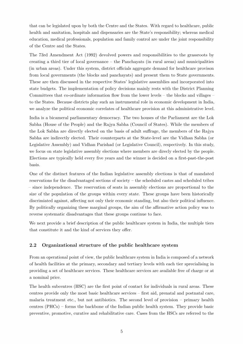
2.2 Organizational structure of the public healthcare system
From an operational point of view, the public healthcare system in India is composed of a network
of health facilities at the primary, secondary and tertiary levels with each tier sprecialising in
providing a set of healthcare services. These healthcare services are available free of charge or at
a nominal price.
The health subcentres (HSC) are the first point of contact for individuals in rural areas. These
centres provide only the most basic healthcare services – first aid, prenatal and postnatal care,
malaria treatment etc., but not antibiotics. The second level of provision – primary health
centres (PHCs) – forms the backbone of the Indian public health system. They provide basic
preventive, promotive, curative and rehabilitative care. Cases from the HSCs are referred to the
5

PHCs with each PHC acting as a referral centre to six HSCs (the lowest tier). It is at the PHCs
that residents in rural areas can access a qualified physician. The community healthcare centres
(CHCs) are referral centres for an average of four PHCs and provide specialist care. The CHCs
are 30-bed hospitals which, in turn, refer out to higher-level sub-divisional or district hospitals.
In this study, we cover different aspects of healthcare provision at the HSCs, PHCs and CHCs
which together serve most of the healthcare needs of the population, particularly of those who
are poor or reside in rural areas.
Table 1 provides an overview of the different components of the Indian public healthcare system:
the main functions they perform, the availability of hospital beds at each tier, the population
covered and their shortfall, the interrelatedness among the tiers and the number of facilities
within each tier. As we can observe from the table, the healthcare system takes the form of
a pyramid with nearly 150 thousand HSCs making the base, a little over 24 thousand PHCs
and about 5 thousand CHCs. The PHCs, as already mentioned, forms the main component,
each serving about 35 thousand people. However, the number of healthcare facilities across the
tiers are much lower than what the government norms provide. Our aim is to investigate the
systematic differences in the provision of healthcare centres, their infrastructure and personnel
from a political economics lens.
Table 1: Coverage of rural health system in India
Avg. pop. covered (in ’000)b
Level Functions Numberof bedsa
Norm Presentstatus
Referredout by
Numberof unitsc
HSC Most peripheral; first point of con-tact between primary healthcare sys-tem and the community in rural areas.
– 3–5 5.6 – 148,366
PHC First point of contact with a qualifiedphysician; provides basic preventative,promotive, curative and rehabilitativecare and act as referral units.
4 to 6 20–30 34.6 6 HSCs 24,049
CHC Block level health administrative unitsand gatekeeper for referrals to higherlevel facilities.
30 80–120 172.4 4 PHCs 4,833
a Source: Rural Health Statistics Bulletin, 2012.b Source: Rural population from Census 2011.c As of March 2012.
Given the diversity of functions they perform, their respective specialisations, the population
they cover, and the number of facilities within each tier, from a political economy perspective it is
reasonable to argue that, at the margin, some services attract more votes than others even though
they are parts of a single healthcare system. These differences in incentives and constraints that
politicians face ultimately determines whether or not a service is actually provided.
In this paper, we investigate how our three main political economy variables – political participa-
tion, electoral compeition, and ENP – are related to different aspects of healthcare provision at
each of the tiers just discussed. In order to get a complete picture we examine the relationship
at different points along the conditional healthcare distribution.
Before we turn to our methodology, we summarise the main elements of the political economy
literature that provides the conceptual background to our study.
6

3 Related literature
3.1 Political economy of healthcare provision
One of the distinguishing features of the healthcare market, as Arrow (1963) insightfully remarked,
is the “existence of uncertainty in the incidence of disease and in the efficacy of treatment”.
The non-marketablity of risk therefore is a distinct feature of the healthcare market. Besides
information gaps, there are other factors that support government intervention in healthcare: it
is regarded as a merit good which ought to be provided on the basis of need and not on the
basis of ability to pay alone; the large externality benefits of healthcare is another factor which
a private market will not consider and hence underprovide healthcare; investments in healthcare
infrastructure such as clinics and hospitals, healthcare research, etc. are public goods which the
private market will under-supply (Glied et al. 2012)
While there is a strong case for government intervention in healthcare, what should be the
optimal level of public provision? One way is to think of governments as benevolent social
planners choosing the optimal level of healthcare that maximizes social welfare. However, this is
not realistic because rational political actors, who decide on the size of provision, face incentives
and constraints. This means that the electoral calculus plays a preeminent role in affecting not
just the size of public provision but also what is publicly provided. The public choice literature,
pioneered by Buchanan and Tullock (1962), provides a positive way forward. Our study is
closely related to the literature on the determinants of local public service delivery. In what
follows, we present some of the main insights from the growing political economy literature to
help formulate our hypotheses.
The political economy literature sees healthcare provision either as a public good that is non-
exclusive and non-rival (Arrow 1963, Mobarak et al. 2011) or as a publicly provided private good
where the beneficiaries can be effectively excluded (see Blomquist and Christiansen 1999, Epple
and Romano 1996b,a, Gouveia 1997, and others). The main predictions from the literature
regarding optimal public provision differs based on whether one views healthcare as a public
good or a publicly provided private good. In the former case, the preferences of the median
voter is pivotal in deciding the size of public provision of healthcare (Downs 1957, Roberts 1977,
Meltzer and Richard 1981). And, in the latter case, under a mixed-provision scheme (i.e. where
both the private and public sectors operate) and where services are excludable, the size of public
provision conforms to the preferences of a lower than median-income household (Epple and
Romano 1996a).3
3.2 Voter engagement, political competition, party fragmentation
Along with theoretical developments, there have been rapid progress in empirical political
economy studies. It is widely accepted that the participation of voters in elections is one of the
“most common and important act citizens take in a democracy” (Aldrich 1993) to the extent that
the legitimacy of democracy and the outcome of elections may be undermined when citizens do
not participate (Lutz and Marsh 2007).
3This arises when the marginal willingness to pay for publicly provided healthcare rises with income.
7

The impact of higher voter participation on economic and developmental outcomes is largely
positive. High levels of voter participation are associated with lower income inequality, a larger
government size but also slower economic growth across a panel of countries (Mueller and
Stratmann 2003). At a cross-country level, Fumagalli and Narciso (2012) find that voter turnout
is the channel through which different forms of government affect economic policies. However,
using night light intensity as an indicator of electricity distribution that politicians can control,
Baskaran et al. (2015) find that voter turnout is not significant in explaining variations in the
log of per capita light or its growth in India, but has a negative impact on the proportion
of lit villages. Another set of literature studies the effect of voting reforms that increase the
franchise on government size. For example, Aidt et al. (2006) find that the extension of franchise
contributed to an increase in government spending in 19th century Western Europe. Husted
and Kenny (1997) find that the abolition of poll taxes and literacy tests increased the scope of
the welfare state in the US. However, enfranchisement of the middle class led to a U-shaped
relationship between voter participation and health related public spending in 19th century
England and Wales (Aidt et al. 2010).
In the Indian context, while a higher voter turnout in a district increases the allocation of nurses
to rural areas of a district, it has no effect on the allocation of doctors and has a negative
effect on the allocation of teachers (Betancourt and Gleason 2000). The argument provided in
the literature is that nurses are less expensive to provide than doctors, but the explanation in
relation to teachers is less clear. In another study examining the factors affecting the number
of schools and teachers and related school infrastructure in villages in North India, the role of
voter turnout is not found to be important (Crost and Kambhampati 2010). With respect to
publicly provided health services in Brazil, clinics and consultation rooms per 1000 people – the
visible public goods – are positively related to turnout but not doctors and nurses (Mobarak
et al. 2011).
Another important political variable that might affect public provision is political competition.
When there is greater contestability of power, policies tend to be more efficient (Aidt and
Eterovic 2011). In closely contested constituencies aligned with the ruling party, elected leaders
provide more electricity and this is positively related to output as measured by the log of per
capita light, its growth and the proportion of lit villages (Baskaran et al. 2015). Higher political
competition is associated with lower public spending in Latin American countries (Aidt and
Eterovic 2011). However, Crost and Kambhampati (2010) find that the effect of a higher margin
of victory, or the difference in vote-share between the winner and runner-up is less clear in the
context of schools in India. It limits the number of middle schools in villages but has no effect on
the number of primary schools and teachers nor on the different school infrastructure parameters
that they study.
In addition, the degree of social fragmentation is known to reduce public provision (see Easterly
and Levine (1997), Alesina et al. (1999), Alesina and La Ferrara (2000), Collier (2000), Miguel
and Gugerty (2005), Habyarimana et al. (2007) etc.). When societies are deeply divided, partisan
preferences become salient. One of the implications of partisan preferences is a greater number of
political parties contesting elections to represent the electorate’s disparate preferences (Neto and
Cox 1997). But whether this translates to reduced public provision depends on the institutional
context and is an open empirical question.
8
In the next section we discuss our main hypotheses relating to the association between each of
the three main political economy covariates and healthcare provision.
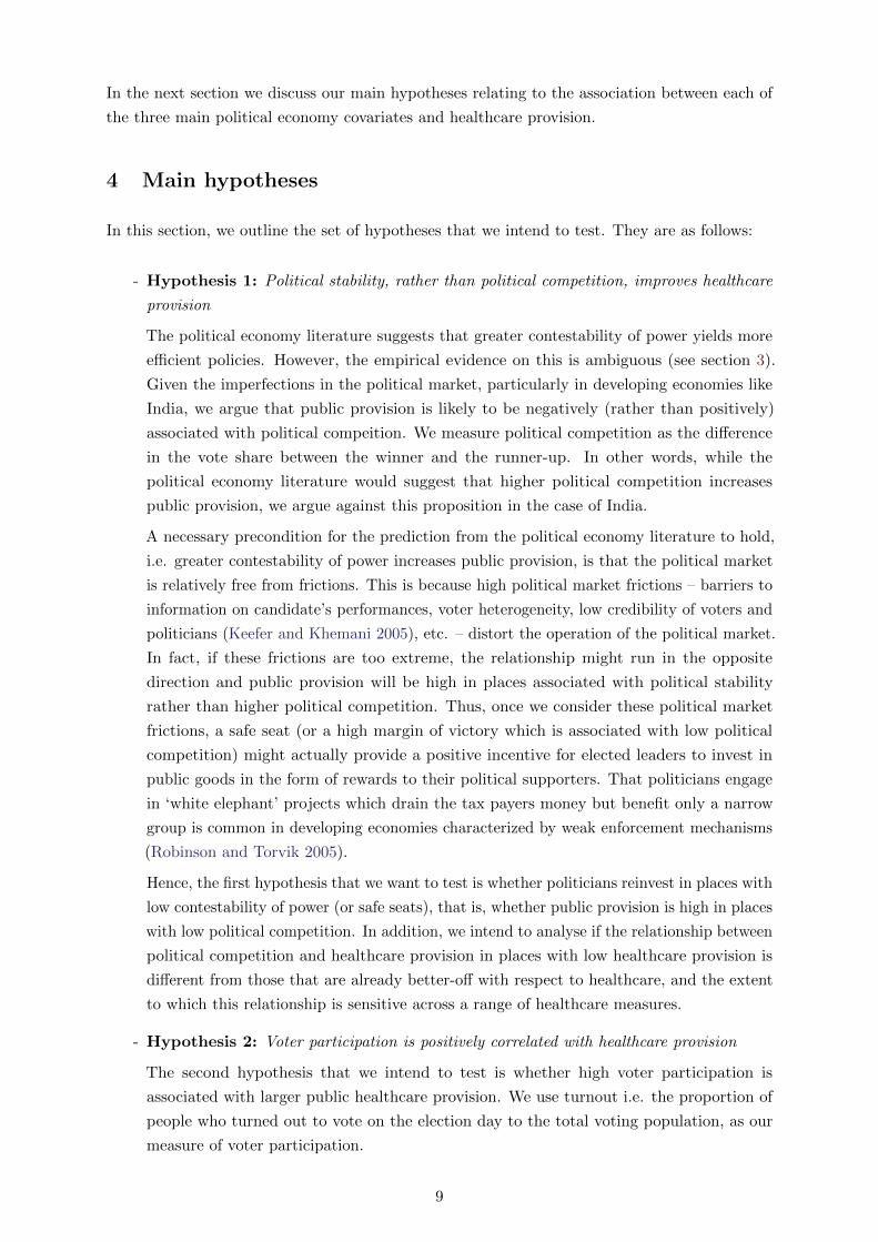
4 Main hypotheses
In this section, we outline the set of hypotheses that we intend to test. They are as follows:
- Hypothesis 1: Political stability, rather than political competition, improves healthcare
provision
The political economy literature suggests that greater contestability of power yields more
efficient policies. However, the empirical evidence on this is ambiguous (see section 3).
Given the imperfections in the political market, particularly in developing economies like
India, we argue that public provision is likely to be negatively (rather than positively)
associated with political compeition. We measure political competition as the difference
in the vote share between the winner and the runner-up. In other words, while the
political economy literature would suggest that higher political competition increases
public provision, we argue against this proposition in the case of India.
A necessary precondition for the prediction from the political economy literature to hold,
i.e. greater contestability of power increases public provision, is that the political market
is relatively free from frictions. This is because high political market frictions – barriers to
information on candidate’s performances, voter heterogeneity, low credibility of voters and
politicians (Keefer and Khemani 2005), etc. – distort the operation of the political market.
In fact, if these frictions are too extreme, the relationship might run in the opposite
direction and public provision will be high in places associated with political stability
rather than higher political competition. Thus, once we consider these political market
frictions, a safe seat (or a high margin of victory which is associated with low political
competition) might actually provide a positive incentive for elected leaders to invest in
public goods in the form of rewards to their political supporters. That politicians engage
in ‘white elephant’ projects which drain the tax payers money but benefit only a narrow
group is common in developing economies characterized by weak enforcement mechanisms
(Robinson and Torvik 2005).
Hence, the first hypothesis that we want to test is whether politicians reinvest in places with
low contestability of power (or safe seats), that is, whether public provision is high in places
with low political competition. In addition, we intend to analyse if the relationship between
political competition and healthcare provision in places with low healthcare provision is
different from those that are already better-off with respect to healthcare, and the extent
to which this relationship is sensitive across a range of healthcare measures.
- Hypothesis 2: Voter participation is positively correlated with healthcare provision
The second hypothesis that we intend to test is whether high voter participation is
associated with larger public healthcare provision. We use turnout i.e. the proportion of
people who turned out to vote on the election day to the total voting population, as our
measure of voter participation.
9

A high turnout reflects more engaged voters. When turnout is high, there is greater
pressure on the politicians to perform. As a result, public provision is likely to be higher
in places where voters are more engaged. The larger the turnout, more involved are the
citizes in local politics and consequently greater is the weight politicians attach to voters’
concerns. On the other hand, apathetic voters are less likely to see their demands converted
into policies.
Voters across the quantiles are likely to demand different things. Thus, in the top quantile,
voters might already have achieved basic healthcare and might prefer more expenditure on
specialised healthcare or even a reduction in the public healthcare provided since they can
easily substitute public with private healthcare providers. The reverse might be true in
the lower quantiles, which are predominantly rural and poorer areas, and where even basic
healthcare is inadequate.
- Hypothesis 3: A broader distribution of political power increases healthcare provision
When previously marginal groups gain prominence in local politics it raises ENP. This
might indicate increasing organizational ability of marginal groups, which in turn, is likely
to improve public provision. India has witnessed a sharp rise in the growth of regional
political parties (Varshney 2000). And this is not necessarily a bad thing. One has to
keep in mind the unprecedented levels of heterogeneity in India compared to any other
democracy. Under such circumstances, a rise in the number of parties might imply an
improvement in the participation of marginal groups in local politics which might then
result in a positive, rather than a negative association, between ENP and healthcare
provision.
On the other hand, if higher ENP is due to increasing social fragmentation, it would be
associated with a reduction in public provision. This is because when opinions are diffuse
and there are multiple social factions, it hinders collective action. Since political parties
choose platforms to represent the preferences of the people, a fragmented electorate is
unlikely to have valence issues which would result in a larger number of parties contesting
on very disparate platforms.
Following Laakso and Taagepera (1979), we construct a measure called the ‘effective
number of parties’ (ENP), as 1∑ni=1 s
2i
where si is the vote share of the ith political party in
a constituency and n is the number of parties contesting elections. If all parties contesting
elections get an equal number of votes, then ENP will equal n. At the other extreme, if
only a single party gets all votes, ENP would be 1. And every other permuation of vote
shares among contesting parties would lie between these two theoretical limits.
Similar to electoral competition and voter participation, discussed above, we are interested
in analysing how ENP affects healthcare provision at different locations along the conditional
healthcare distribution and across a set of healthcare measures.
We discuss our methodology to test these hypotheses in the next section.
10

5 Methodology
The main empirical challenge in examining the relationship between political economy variables
and healthcare is that the association between them at the lower quantiles may be different
than at the higher quantiles (see Figure 1 above). The conventional least squares estimates
focus on the average effect of the explanatory variables on healthcare provision. However,
when the variables are heterogeneous, regressions focusing on the average effect might under or
overestimate effects or even fail to identify effects (Cade and Noon 2003).
In this study, we consider 8 separate healthcare variables: 2 relating to access, and 6 relating to
capacity – one for healthcare infrastructure and another for healthcare personnel and training
over three levels – the HSCs, the PHCs, and the CHCs. The statistical tests clearly indicate
that the conditional distributions of all the 8 variables are non-normal and heteroscedasticity is
a problem in 6 out of the 8 variables.4 The results are presented in Table 10 in Appendix B.1.
The heterogeneity and non-normality of the conditional distributions (OLS residuals) from
statistical tests affirm the need to closely examine the association between political economy
variables and healthcare provision at the extremes: at the lower end, where provision is exceedingly
low, and at the higher end, where healthcare provision is much higher. One way to study this
is to examine the coefficents of the political economy variables at different locations along the
conditional healthcare distributions.
We use the quantile regression model, introduced by Koenker and Bassett (1978) to estimate the
differential impact of the political economy variables on the conditional healthcare distribution.
We model the association at the τ th quantile as:
Qτ (y|x, z) = x′β(τ) + z′γ(τ) (1)
where y, the dependent variable, measures publicly provided healthcare. The quantile function,
Q(.), is linear in the political economy variables – the vector x and their corresponding quantile-
specific coefficients, β, which are our main interest – and a vector, z, that controls for potential
confounding factors like mandated representation in politics, socio-economic, demographic and
geographic differences across the districts in our study. γ contains the corresponding coefficient
estimates for the set of controls included in the model.
The quantile regression model minimizes the sum of errors, weighted by an asymmetric absolute
loss function to estimate quantile-specific coefficients. Mathematically, quantile regression solves
the following optimization problem:
arg minβ,γ
1
n
n∑i=1
ρτ (y − x′iβ − z′iγ) (2)
which can be rewritten as:
arg minβ,γ
1
n
n∑i=1
ρτ (ui) (3)
4We run the Shapiro-Wilk test for normality and White’s heteroscedasticity test on OLS residuals with fullmodel specification. The empirical specification is discussed in Section 6.2.
11

where τ ∈ (0, 1), and ρτ (u) = u(τ − Iu≤0) is a piecewise linear and asymmetric absolute
loss function (or “check ” function) (Koenker and Hallock 2001). The penalty from straying
away from a specific quantile increases with distance in either direction, positive or negative,
which is controlled by ρτ (u).5 As the objective function is not differentiable (at u = 0), linear
programming based algorithms are used in its optimization.6
A different approach to this problem would be to create sub-samples depending on whether
healthcare provision is low or high and running separate regressions. This however raises two
important issues: first, focusing on smaller subsamples is not efficient in the use of available
information. Secondly, sampling on the dependent variable raises concerns regarding sampling
selection bias as the subsamples may be inherently different. The advantage of using quantile
regression is that it uses the entire dataset by weighting the conditional distribution differently
depending on how far they are from a specific quantile, and thereby avoids both these concerns.
Heteroscedasticity is also a problem in quantile regressions. A linear homoscedastic model
would assume that the conditional distribution of healthcare provision is no more spread out
for politically ‘active’ areas than for areas that are politically ‘dormant’. In homoscedastic
conditional quantile functions, the coefficients across the quantiles would only see a ‘location’ shift
i.e. only the intercepts would change, whereas, heteroscedasticity would imply a ‘location-scale’
shift (Koenker 2005). Quantile regressions often assume that errors are i.i.d. and that the model
is correctly specified. Misspecified models invalidate inferences based on conventional covariance
matrix (Kim and White 2003) and i.i.d. errors are quite restrictive. Powell (1994), Kim and
White (2003) and others have derived asymptotic properties when errors are independent but
not identically distributed and quantile regressions are possibly misspecified (Machado and Silva
2013).7
We test for heteroscedasticity at the conditional quantiles using the Machado and Silva (2000)
test. The results in Table 11 in Appendix B.2 shows that heteroscedasticity is present in a
large majority of the cases we study. Since heteroscedasticity might bias our inferences of the
estimates, we present standard errors in the regression tables that are robust to heteroscedasticity
and misspecification bias.
Quantile regression is a semi-parametric approach wherein, similar to OLS, the linearity assump-
tion is maintained but differs from it by considering the entire conditional distribution and not
just the average effect (Powell 1994). Because of this, we are able to investigate the differential
effect of a 1% point increase in the political economy variables at different points along the
conditional healthcare distribution.
In the next section, we introduce our data and describe the specification of our econometric
models.
5ρτ (u) asymmetrically weights positive and negative terms as: I(u > 0).τu+ I(u ≤ 0).(1 − τ)u6An alternative estimation approach is to smooth the ‘cusp’ of the ‘check’ function to allow computational
techniques relying on differentiability (see Jung et al. 2015, and references therein)7This is implemented in Stata using the ‘qreg2’ package developed by MSS 2011
12

6 Data and empirical specification
6.1 Data set and variable selection
In order to examine the political economy of publicly provided healthcare in India we created
a dataset that combines information on healthcare provision, electoral results, socio-economy,
demography and geography. Our sample consists of district-level observations for 15 major
Indian states. Table 2 provides summary statistics.
One of the most time-intensive pre-analysis exercise was to reconstruct the district boundaries to
match that of the 2001 census year. Because district boundaries change over time, it was essential
that we maintained uniform district boundaries across the different data sources. Appendix A
describes the procedure adopted to obtain district-level election variables by matching election
results for every constituency to their respective districts. Once they were matched, we had 430
districts in our sample covering 15 major Indian states.
Table 2: Summary statisticsVariable Obs Mean Std. Dev. Min Max p10 p25 p50 p75 p90
Fraction of villages in a district having:HSC - access 430 .41 .21 0 1 .21 .27 .37 .5 .68PHC - access 430 .14 .2 0 1 .02 .04 .08 .14 .24
Fraction of health centres in a district having:Infrastructure capacity:HSC - labour room 430 .35 .25 0 1 .02 .13 .33 .52 .7PHC - labour room 428 .69 .28 0 1 .25 .5 .78 .89 1CHC - ambulance 422 .67 .29 0 1 .27 .5 .73 1 1Human resource capacity:HSC - trained nurses 430 .31 .2 0 1 .08 .17 .28 .43 .56PHC - female doctors 428 .27 .28 0 1 0 .04 .2 .41 .7CHC - general surgeon 422 .29 .28 0 1 0 0 .24 .45 .67
Political variables:Vote margin 430 .16 .05 .05 .4 .1 .12 .15 .18 .21Turnout 430 .61 .09 .37 .81 .49 .54 .6 .68 .73ENP 430 2.63 .44 1.73 4.06 2.13 2.3 2.56 2.89 3.26SC seat 430 .16 .14 0 1 0 0 .15 .23 .33ST seat 430 .08 .22 0 1 0 0 0 0 .33
Socio-economy:Literacy 430 .63 .12 .31 .96 .47 .56 .63 .72 .77Log pop. 430 14.38 .6 12.14 16.08 13.63 13.99 14.37 14.8 15.1Pop. growth 430 .21 .08 .04 .55 .1 .15 .22 .26 .3Urban pop. 430 .22 .15 0 .88 .07 .11 .19 .29 .44Log income 422 1.92 1.91 0 17.5 .59 .91 1.61 2.32 3.34
Geography:Log Area 430 8.43 .68 6.09 10.73 7.59 7.95 8.41 8.92 9.29Dist. from equator 430 .25 .06 .09 .36 .14 .21 .26 .29 .32
Data source: Own calculation using data from DLHS-3 (2007-8), Census of India (2001), ECI (1977-1999)
G-Econ (2000) and GADM.
6.1.1 Measures of healthcare provision
We obtained data on access to health facilities, its infrastructure and human resource capacities
at health centres from district-level reports of the third round of the District Level Household
and Facility Survey (DLHS-3), 2007-08. Our dependent variables – the different measures of
publicly provided healthcare at the district level – come from this dataset. We examine a
total of 8 healthcare variables: 2 relate to access and 6 relate to capacity – one for healthcare
infrastructure and another for healthcare personnel and training over three levels – HSCs, PHCs,
and CHCs.
13
The reason behind examining multiple healthcare variables needs to be explained. Access to
healthcare is the most fundamental of all the healthcare measures. Given that the different tiers
of the healthcare system perform very different functions, we examine access to HSCs and PHCs
separately but not CHCs because the first two provide the bulk of the healthcare services that
are most commonly accessed.
Besides access, healthcare infrastructure and human resource capacity affects healthcare service
delivery. These present different incentives and contraints to the politicians which might
systematically affect their provision. Firstly, healthcare services are not equally visible. For
example, Mani and Mukand (2007) and Mobarak et al. (2011) show that more visible goods (e.g.
buildings) take priority over less visible ones (e.g. doctors and nurses). A related point is that
certain aspects of healthcare are associated with higher levels of treatment-uncertainty than
others which affects their demand (Arrow 1963).
Secondly, not all healthcare services are flexible enough that a politician can change its provision
within her tenure in office. For example, when doctors and nurses are not adequately trained,
it takes concerted action across several departments to improve training and not just political
will. In addition, certain aspects of healthcare provision are more likely to be influenced by
government norms which reduces the politicians’ scope to affect change. Thirdly, healthcare
service delivery is prone to ratchet effects. So, while doctors and nurses are hired during good
times, it is the supplies and training that are reduced during cut-backs (Kremer and Glennerster
2011). This is because restructuring of personnel faces stiff political opposition whereas supplies
can be easily reduced.
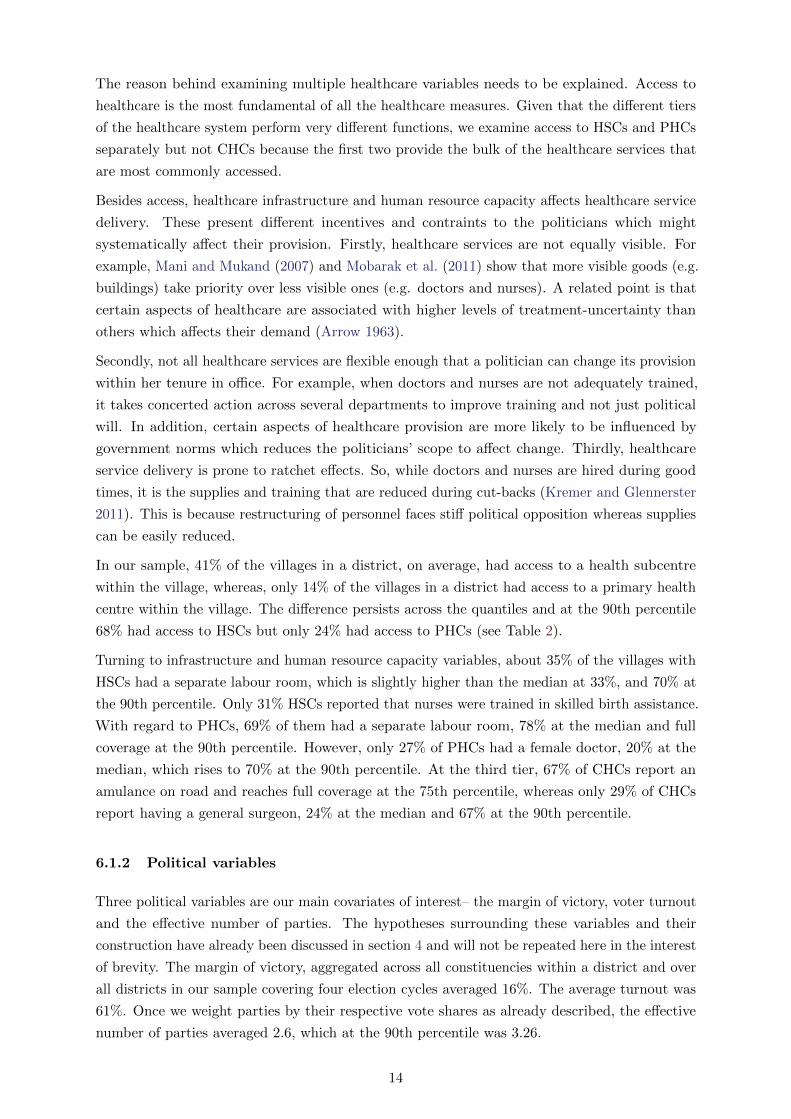
In our sample, 41% of the villages in a district, on average, had access to a health subcentre
within the village, whereas, only 14% of the villages in a district had access to a primary health
centre within the village. The difference persists across the quantiles and at the 90th percentile
68% had access to HSCs but only 24% had access to PHCs (see Table 2).
Turning to infrastructure and human resource capacity variables, about 35% of the villages with
HSCs had a separate labour room, which is slightly higher than the median at 33%, and 70% at
the 90th percentile. Only 31% HSCs reported that nurses were trained in skilled birth assistance.
With regard to PHCs, 69% of them had a separate labour room, 78% at the median and full
coverage at the 90th percentile. However, only 27% of PHCs had a female doctor, 20% at the
median, which rises to 70% at the 90th percentile. At the third tier, 67% of CHCs report an
amulance on road and reaches full coverage at the 75th percentile, whereas only 29% of CHCs
report having a general surgeon, 24% at the median and 67% at the 90th percentile.
6.1.2 Political variables
Three political variables are our main covariates of interest– the margin of victory, voter turnout
and the effective number of parties. The hypotheses surrounding these variables and their
construction have already been discussed in section 4 and will not be repeated here in the interest
of brevity. The margin of victory, aggregated across all constituencies within a district and over
all districts in our sample covering four election cycles averaged 16%. The average turnout was
61%. Once we weight parties by their respective vote shares as already described, the effective
number of parties averaged 2.6, which at the 90th percentile was 3.26.
14

To add to these variables we include the institutional mandate of reservation of seats for the
disadvantaged sections of society – the scheduled castes and scheduled tribes – in our models.
We cover four election cycles spanning 1977-1999 to capture the longer-term impact of political
forces on healthcare provision. Because elections are held once in 5 years, and states are on
different election cycles, we effectively leave out two and in some cases one election cycle between
the period upto which we consider to construct our political variables and the DLHS-3 survey.
We outline our model specification next.
6.2 Empirical Specification
We estimate the τ th conditional quantile function for healthcare measure k in district i, Q(hik),
as:
Q(hik|x, z) = α(τ) + β1(τ)Ti + β2(τ)Vi + β3(τ)ENPi + γ(τ)Zi (4)
where,
- Ti = Voter turnout;
- Vi = Margin of victory;
- ENPi = Effective number of parties;
- Zi = vector of control variables.
βj(τ), j = {1, 2, 3} are the corresponding coefficient vectors; α(τ) is a constant; Zi is a vector of
district-specific controls and the proportion of seats reserved for SCs and STs in a district with
coefficients in γ. Our main interest, as laid out in Section 4, are the coefficients βj(τ)s which
capture the marginal impact of the jth political economy variable on healthcare provision, k, at
the τ th conditional quantile.
The healthcare variables that we observe today are the outcome of the cumulative impact of
policy decisions over time. Here, we are primarily interested in the longer-term impact of political
forces on healthcare provision and not on the political flavour in a single election year. Because
changes in healthcare variables have been accumulating over a considerable period of time, it will
be unreasonable to associate only the current political market forces with observed distributions
of healthcare since it is not only the present but also past policies that have shaped current
healthcare. Further, in an econometric analysis, using current political economy variables to
explain healthcare will result in simultaneity bias as the political variables themselves will be
affected by healthcare conditions. To minimize this problem, and to look at the longer-term
impact of political forces, we aggregate district averages across roughly four election cycles
spanning 1977-1999.
In addition to the the three main political economy variables – voter participation, electoral
competition and ENP – we also include variables to control for the share of seats for SCs and
STs, and other district level heterogeneity that might confound our results. Specifically, we
control for a district’s literacy rate, the natural logarithm of population, population growth, the
15

percentage of urban population and the natural logarithm of output. Since a district’s income
influences its ability to spend on public healthcare, we included data on output. To do this, we
obtained gridded data on output for the year 2000 from the G-Econ database.8. Except output,
socio-economic data was obtained from the 2001 census year.
Because geography determines a region’s natural susceptibility to a disease which might affect
healthcare provision, we include a district’s latitude to control for possible differences in disease
incidence. Using latitude to capture disease incidence is well-established in the economic growth
literature (see Gallup et al. 1999, Hall and Jones 1999, Easterly and Levine 2003, Spolaore and
Wacziarg 2013, and others). We also control for a district’s area to net out any economies of scale
that might arise in providing healthcare. Finally, we include dummies to control for regional
effects that might arise due to shared culture, languages or other unobservable attributes.
To minimize simultaneity bias, we lagged political economy variables and controls. This ensures
that the direction of influence runs from political variables to public provision of healthcare and
not the other way round.9
In this paper, we are concerned with examining the association between political economy vari-
ables and provision of healthcare at different points along the conditional healthcare distribution,
after controlling for potential confounding factors. Hence, our results are to be interpreted
as associations and not as causal effects of the political economy variables. Our aim here is
to extend our understanding of the association at the extremes of the conditional healthcare
distrbution i.e. either when healthcare provision is excedingly low, or when it is remarkably
high.
We discuss our empirical findings in the next section.
7 Results
Based on the empirical specification in eq.(4) we test the three main hypotheses outlined before
in section 4. They are: (a) political stability, rather than political competition, is associated with
improved healthcare provision; (b) voter participation is positively correlated with healthcare
provision; and (c) a broader distribution of political power, measured by ENP, is associated with
improved healthcare provision. Because the relationship between political economy variables and
healthcare provision might be different when healthcare provision is severly deficient than when
it is much higher, we use quantile regression to obtain values of marginal impact at different
points along the conditional healthcare distribution.
We report our findings in Tables 3, 4 and 5. To obtain robust inferences, we report standard
errors that are robust to heteroscedasticity and potential misspecifications.
Table 3 reports results relating to healthcare access, Table 4 on healthcare infrastructure, and
Table 5 on healthcare personnel and training. These tables consist of separate panels each
reporting estimates relating to a specific dependent variable and the Pseudo-R2s corresponding
8Gridded data on the value of output at 1◦ by 1◦ resolution was obtained from the G-Econ project available athttp://gecon.yale.edu/. The grid was then overlaid onto district boundaries and the value of output of thegrid overlaying the district centroid was taken to represent the value of output for that district.
9However, to the extent that there is path dependence in health care provision, the issue of endogeneity willnot be completely addressed.
16

to quantiles 10, 25, 50, 75 and 90, in separate columns. We also include OLS results in the
first column. The rows, in every panel, are our main political variables of interest – margin
of victory, turnout and ENP. For example, Panel C in Table 4 presents the quantile-specific
impact of political economy variables on having labour rooms at PHC. At the 10th quantile,
a one standard deviation increase in the margin of victory (the standard deviation of margin
of victory is obtained from Table 2) would be associated with a 8% point (=0.05*1.594, the
coefficient 1.594 is from Panel B in Table 4) increase in having a labour room at PHC. Computed
in the same way, a one standard deviation increase in turnout would be associated with over a
9% point (=0.09*1.044) increase, whereas a one standard deviation increase in ENP would be
associated with almost a 7% point (=0.44*0.155) increase.
We discuss our results below. For the ease of exposition, we group the discussion of the results
around the three main hypotheses which we have already outlined.
Table 3: Factors affecting healthcare access
Variable name OLS Q(0.10) Q(0.25) Q(0.50) Q(0.75) Q(0.90)
Panel A: Access to HSCVote margin -0.369 0.056 0.064 -0.169 -0.236 -0.239
(0.235) (0.250) (0.193) (0.264) (0.341) (0.209)Turnout -0.154 -0.142 -0.019 0.094 -0.049 -0.068
(0.138) (0.130) (0.118) (0.199) (0.175) (0.294)ENP -0.111∗∗∗ -0.047∗ -0.034 -0.068∗∗ -0.132∗∗∗ -0.179∗∗∗
(0.024) (0.027) (0.022) (0.030) (0.037) (0.042)
R2 .29 .11 .159 .254 .266 .224
Panel B: Access to PHCVote margin -0.598∗∗ 0.033 0.121 -0.030 -0.390 -0.430∗
(0.258) (0.096) (0.089) (0.098) (0.461) (0.234)Turnout -0.567∗∗∗ -0.114∗ -0.107 -0.172∗∗ -0.228 -0.150
(0.136) (0.064) (0.072) (0.072) (0.155) (0.132)ENP -0.094∗∗∗ -0.001 -0.016 -0.036∗∗∗ -0.045 -0.052∗∗∗
(0.023) (0.008) (0.012) (0.012) (0.028) (0.020)
R2 .35 .146 .173 .22 .323 .233
Notes: ∗ p < 0.1, ∗∗ p < 0.05, ∗∗∗ p < 0.01; N=422 in both Panels A and B. The table shows the marginal effects ofour main covariates on the conditional distribution of different quantiles of healthcare access, where access is measuredas the proportion of villages within a district with health sub-centres (Panel A) and primary healthcare centres (PanelB). All regressions include the proportion of seats in a district reserved for scheduled castes and scheduled tribes anddistrict-specific controls: literacy rate, log. of population, population growth, percentage of urban population, log. ofincome, area, and latitude. We also include regional dummies in every regression. Standard errors in parenthesis arerobust to heteroscedasticity for OLS models and robust to heteroscedasticity and misspecification bias for quantileregressions. Reported R2s for quantile regressions are the square of the correlation between the fitted values and thedependent variables.
7.1 The effect of political competition
In the case of 5 out of 8 dependent variables we find that a low level of political competition (or
equivalently a high margin of victory) is associated with an increase in healthcare provision. Thus,
political competition has a largely negative (rather than a positive) impact on healthcare provision
in India. This effect-size varies across quantiles and also over the different variables we study.
Its effect is positive and most pronounced with respect to capacity variables – infrastructure
(Table 4) and personnel and training of doctors and nurses (Table 5) – except having general
surgeons at CHC, whereas, it is not statistically significantly associated with healthcare access
(Table 3), except at the 90th quantile for PHC access, where it is, in fact, negative.
17

Table 4: Factors affecting healthcare infrastructure
Variable name OLS Q(0.10) Q(0.25) Q(0.50) Q(0.75) Q(0.90)
Panel A: HSC - Separate labour roomVote margin 0.422 0.523∗∗ 0.076 0.160 0.768∗ 0.975∗∗
(0.279) (0.211) (0.280) (0.415) (0.408) (0.473)Turnout -0.415∗∗ 0.023 0.126 -0.311 -0.223 -0.303
(0.173) (0.197) (0.220) (0.211) (0.202) (0.318)ENP 0.130∗∗∗ 0.028 0.033 0.108∗ 0.153∗∗∗ 0.155∗∗
(0.035) (0.030) (0.033) (0.056) (0.049) (0.066)
R2 .277 .141 .157 .25 .209 .154
Panel B: PHC - Separate labour roomVote margin 0.954∗∗∗ 1.594∗∗∗ 1.055∗∗ 0.532 0.557 -0.016
(0.310) (0.527) (0.457) (0.489) (0.353) (0.351)Turnout 0.554∗∗∗ 1.044∗∗∗ 0.916∗∗∗ 0.512∗∗ 0.327 0.072
(0.181) (0.330) (0.303) (0.214) (0.211) (0.213)ENP 0.101∗∗∗ 0.155∗∗∗ 0.089∗ 0.048 0.031 -0.017
(0.034) (0.057) (0.049) (0.039) (0.043) (0.030)
R2 .369 .332 .321 .325 .293 .233
Panel C: CHC - Ambulance on roadVote margin 1.320∗∗∗ 0.762 1.052∗∗ 1.448∗∗∗ 1.732∗∗∗ 0.459∗
(0.334) (1.082) (0.528) (0.501) (0.324) (0.243)Turnout 0.749∗∗∗ 1.037∗ 0.942∗∗∗ 0.637∗∗∗ 0.717∗∗∗ 0.166
(0.200) (0.538) (0.345) (0.242) (0.213) (0.155)ENP 0.091∗∗ 0.039 0.060 0.077 0.128∗∗∗ 0.033
(0.042) (0.083) (0.089) (0.056) (0.046) (0.037)
R2 .199 .122 .179 .189 .14 .103
Notes: ∗ p < 0.1, ∗∗ p < 0.05, ∗∗∗ p < 0.01; N=422 in Panel A, N=420 in Panel B, and N=415 in Panel C. Allregressions include the proportion of seats in a district reserved for scheduled castes and scheduled tribes and district-specific controls: literacy rate, log. of population, population growth, percentage of urban population, log. of income,area and latitude. We also include regional dummies in every regression. Standard errors in parenthesis are robust toheteroscedasticity for OLS models and robust to heteroscedasticity and misspecification bias for quantile regressions.Reported R2s for quantile regressions are the square of the correlation between the fitted values and the dependentvariables.
18

Table 5: Factors affecting healthcare personnel and training
Variable name OLS Q(0.10) Q(0.25) Q(0.50) Q(0.75) Q(0.90)
Panel A: HSC - ANM attended skilled birth training within last 5 yearsVote margin 0.297 0.669∗∗ 0.638∗∗ 0.096 0.561 0.690∗∗
(0.231) (0.318) (0.262) (0.245) (0.365) (0.346)Turnout -0.525∗∗∗ 0.321∗ -0.068 -0.528∗∗∗ -0.869∗∗∗ -1.116∗∗∗
(0.147) (0.181) (0.225) (0.165) (0.168) (0.180)ENP 0.045 0.049∗ 0.040 0.048 0.036 0.090∗∗∗
(0.027) (0.029) (0.033) (0.034) (0.040) (0.034)
R2 .231 .0633 .166 .221 .207 .186
Panel B: PHC - Female medical officerVote margin 0.571 0.409 0.818∗∗∗ 1.011∗∗ 1.420∗∗∗ 1.169∗∗∗
(0.374) (0.279) (0.243) (0.442) (0.476) (0.434)Turnout 0.129 0.220 0.414∗∗ 0.586∗∗ 0.038 0.577
(0.195) (0.150) (0.160) (0.294) (0.312) (0.388)ENP -0.004 0.022 0.047∗ 0.040 -0.008 0.024
(0.033) (0.024) (0.026) (0.030) (0.054) (0.053)
R2 .262 .114 .142 .217 .239 .168
Panel C: CHC - has a general surgeonVote margin -0.901∗∗ -0.215 -0.752∗∗ -1.715∗∗∗ -1.911∗∗∗ 0.141
(0.429) (0.278) (0.353) (0.429) (0.642) (0.434)Turnout -0.876∗∗∗ -0.332∗ -0.761∗∗∗ -1.038∗∗∗ -0.831∗ -0.314
(0.241) (0.196) (0.231) (0.276) (0.459) (0.503)ENP -0.131∗∗∗ -0.017 -0.043 -0.156∗∗∗ -0.232∗∗∗ -0.078
(0.039) (0.042) (0.037) (0.060) (0.055) (0.083)
R2 .141 .0645 .054 .0924 .106 .0649
Notes: ∗ p < 0.1, ∗∗ p < 0.05, ∗∗∗ p < 0.01; N=422 in Panel A, N=420 in Panel B, and N=415 in Panel C. Allregressions include the proportion of seats in a district reserved for scheduled castes and scheduled tribes and district-specific controls: literacy rate, log. of population, population growth, percentage of urban population, log. of income,area and latitude. We also include regional dummies in every regression. Standard errors in parenthesis are robust toheteroscedasticity for OLS models and robust to heteroscedasticity and misspecification bias for quantile regressions.Reported R2s for quantile regressions are the square of the correlation between the fitted values and the dependentvariables.
19

With respect to having labour rooms at HSC (see Panel A in Table 4), political competition is
associated with a reduction in its provision. The (negative) association with political competition
is small in size at lower quantiles, but increases as we move towards higher quantiles i.e. when
its provision is also high. In Panel B of the same table, political competition is negatively
associated with having labour room at PHC, like in the case of HSC, but differs in that the
coefficients become smaller in magnitude as we move towards higher quantiles before losing
statistical significance. For those quantiles where the effect of vote margin on having ambulance
at CHC is statistically significant, it is positive (i.e. exhibits a negative association with political
competition), but declines as we consider higher quantiles (see Panel C in the same table).
This is also true for nurses trained in birth assistance at HSC (Panel A in Table 5) and female
doctors at PHC (Panel B in Table 5), although the association is stronger in the case of female
doctors, where the effect size is inverted-U shaped (see Figure 2).
Neither access to HSC nor PHC (Panels A and B respectively, in Table 3) is statistically
significant with respect to margin of victory. However, to the extent that there is any significant
effect, its impact is negative indicating that higher vote margin is associated with an increase
in provision but only at the top-most quantile which already enjoys better access than the
remaining 90% of the sample. The effect of political competition is also positive with respect
to having general surgeon at CHC (Panel C in Table 5) although its effect is much larger at
lower quantiles, dips at the median, and rises again at higher quantiles before losing statistical
significance (see Panel C in Table 5). This is not at all surprising. The norms surrounding
access to healthcare are well-defined and its provision to a large extent depends on whether an
area falls short of those pre-specified norms (see Table 1). Thus, relative to other healthcare
variables we consider, politicians may not have a great degree of manoeuvreability in affecting
change when it comes to access, which explains why they are not statistically significant. But
when they are, as in the case of PHC access, the coefficient is negative and access is positively
associated with increasing political competition.
As already mentioned, political market frictions such as information constraints on candidate
performances, low enforcement of election promises, etc., impede greater political competition
from increasing public provision. When political market frictions are high, there is a strong
incentive for polticians to reinvest in ‘safe’ seats by increasing public provision (i.e. when margin
of victory is high). This might be why we find the association to be positive in 5 out of the 8
dependent variables we study, that is, in these instances political stability rather than political
competition is associated with improved healthcare provision.
In Figure 2, we plot the association between vote margin and our set of dependent variables at
different quantiles. In all cases (except having general surgeons at CHC) the effect at the 10th
quantile is positive. However, as already discussed above, the impact is heterogeneous across
quantiles reinforcing the importance of examining the effect of our covariates along the entire
distribution rather than just at the mean.
7.2 The effect of voter turnout
The percentage of people who actually turned out to vote is representative of how engaged
voters are with politics. One would expect public provision to be positively associated with
20

−1.0
0
−0.5
0
0.00
0.50
1.00
.1.25 .5 .75.9Quantile
HSC−access
−1.0
0
−0.5
0
0.00
0.50
.1.25 .5 .75.9Quantile
PHC−access
−0.5
0
0.00
0.50
1.00
1.50
2.00
.1 .25 .5 .75 .9Quantile
HSC−labour−room
−0.5
0
0.00
0.50
1.00
1.50
2.00
.1 .25 .5 .75 .9Quantile
PHC−labour−room
−1.0
0
0.00
1.00
2.00
3.00
.1 .25 .5 .75.9Quantile
CHC−ambuance
−0.5
0
0.00
0.50
1.00
1.50
2.00
.1 .25 .5 .75 .9Quantile
HSC−trained−nurse
−1.0
0
0.00
1.00
2.00
3.00
.1 .25 .5 .75 .9Quantile
PHC−female−doctors
−3.0
0
−2.0
0
−1.0
0
0.00
1.00
.1 .25 .5 .75 .9Quantile
CHC−general−surgeon
Figure 2: The figure shows the marginal effect of victory margin on healthcare provisionacross different quantiles based on bootstrapped regressions with 100 replications. Each panelcorresponds to one of the 8 healthcare measures.
turnout because higher voter engagement means greater political pressure and stricter political
accountability.
The impact of turnout is, however, heterogeneous across variables and also across quantiles.
Like margin of victory, turnout is positively correlated with having labour room at PHC, having
ambulance at CHC (Panels B and C in Table 4) and having female doctors at PHC (Panel B in
Table 5) but is negatively associated with access to PHC (Panel A in Table 3), trained nurses at
HSC and general surgeons at CHC (Panels A and C in Table 5).
The strength of the positive association between turnout and having labour room at PHC
declines as we move to higher quantiles. For female doctors at PHC, the impact is positive and
significant only at the 25th and 50th quantiles and is not significant elsewhere. With regard to
ambulance at CHC, the effect declines gradually, and loses statistical significance thereafter (see
Figure 3).
Turnout has no discernible impact on access to HSC (Panel A, Table 3) or labour rooms at HSC.
This is expected. HSC have relatively high coverage: 41% of districts in our sample reported
having access to HSC which increased to 68% at the 90th quantile. By contrast, only 14% of the
districts reported having access to PHC and 24% at the 90th quantile.
In Figure 3, we plot the association between turnout and our set of dependent variables at
different quantiles which again highlights the differential impact of turnout along the healthcare
distributions. It is positively associated with 3 out of 8 dependent variables, an equal number for
which the association is negative, and not significant for the remaining two variables. Therefore,
21

our hypothesis that turnout is positively associated with healthcare provision holds only for a
subset of variables.
−0.5
0
0.00
0.50
.1.25 .5 .75.9Quantile
HSC−access
−0.8
0−0
.60
−0.4
0−0
.20
0.00
0.20
.1.25 .5 .75.9Quantile
PHC−access
−1.5
0
−1.0
0
−0.5
0
0.00
0.50
.1 .25 .5 .75 .9Quantile
HSC−labour−room
−0.5
0
0.00
0.50
1.00
1.50
.1 .25 .5 .75 .9Quantile
PHC−labour−room
−1.0
0
0.00
1.00
2.00
3.00
.1 .25 .5 .75.9Quantile
CHC−ambuance
−1.5
0
−1.0
0
−0.5
0
0.00
0.50
.1 .25 .5 .75 .9Quantile
HSC−trained−nurse
−1.5
0−1
.00
−0.5
0
0.00
0.50
1.00
.1 .25 .5 .75 .9Quantile
PHC−female−doctors
−1.5
0−1
.00
−0.5
0
0.00
0.50
.1 .25 .5 .75 .9Quantile
CHC−general−surgeon
Figure 3: The figure shows the marginal effect of turnout on healthcare provision across differentquantiles based on bootstrapped regressions with 100 replications. Each panel corresponds toone of the 8 healthcare measures.
7.3 The effect of ENP
We measure party fragmentation by the effective number of parties (ENP) which is the inverse of
the sum of vote shares across all parties contesting elections. By weighting the parties by their
vote shares, a high value for ENP indicates a broader distribution of political power. Its impact
is hard to predict ex-ante. This is because ENP can be high when smaller groups are able to
organize themselves politically. Anecdotal evidence on the growth of regional parties in India
would suggest a broadening of the distribution of political power (see Varshney 2000) which
would result in high ENP without a change in the underlying social divisions. If this is indeed
the case, the association between ENP and healthcare provision is expected to be positive. On
the other hand, a high ENP might indicate a heterogeneous society in which case the coefficient
will have a negative sign.
We find that higher ENP is largely associated with an increase in healthcare provision with
considerable heterogeneity across the variables and quantiles. Higher ENP or an increase in
the effective number of parties is positively associated with a rise in having labour rooms at
HSC and PHC (Panels A and B in Table 4). The association is also positive with respect to
having trained nurses and female doctors at HSC and PHC respectively (Panels A and B in
Table 5) and having ambulance at CHC (Panel C in Table 4). However, barring a few exceptions,
its impact is statistically significant mostly at the higher quantiles. The positive association
22

between ENP and healthcare provision, in spite of controlling for the share of seats reserved for
scheduled castes and for scheduled tribes in all our regressions is consistent with the (anecdotal)
observation that smaller groups have increasingly organized themselves politically (without an
increase in the underlying social heterogeneity) which might be why ENP is positively associated
with healthcare provision.
With respect to access to HSCs and PHCs (Panels A and B in Table 3), and surgeons at CHCs
(Panel C in Table 5) the association with ENP is negative. This is because whether or not a
village has a local healthcare facility is largely influenced by government norms on coverage (see
Table 1), whereas, CHCs, being more remote from most people are less electorally crucial.
In Figure 4, we plot the association between ENP and our set of dependent variables at different
quantiles. Similar to margin of victory and turnout, the impact of ENP is heterogeneous across
quantiles and over the different dependent variables we study.
−0.3
0
−0.2
0
−0.1
0
0.00
0.10
.1.25 .5 .75.9Quantile
HSC−access
−0.1
5
−0.1
0
−0.0
5
0.00
.1.25 .5 .75.9Quantile
PHC−access
−0.1
0
0.00
0.10
0.20
0.30
.1 .25 .5 .75 .9Quantile
HSC−labour−room
−0.0
50.
000.
050.
100.
150.
20
.1 .25 .5 .75 .9Quantile
PHC−labour−room
−0.1
0
0.00
0.10
0.20
0.30
.1 .25 .5 .75.9Quantile
CHC−ambuance
−0.0
5
0.00
0.05
0.10
0.15
0.20
.1 .25 .5 .75 .9Quantile
HSC−trained−nurse
−0.1
5−0
.10
−0.0
5
0.00
0.05
.1 .25 .5 .75 .9Quantile
PHC−female−doctors
−0.3
0
−0.2
0
−0.1
0
0.00
0.10
.1 .25 .5 .75 .9Quantile
CHC−general−surgeon
Figure 4: The figure shows the marginal effect of ENP on healthcare provision across differentquantiles based on bootstrapped regressions with 100 replications. Each panel corresponds toone of the 8 healthcare measures.
To summarize, we find that the margin of victory is positively associated with 5 out of 8
healthcare variables which implies that it is political stability rather than political competition
that is associated with improved healthcare provision. The effect of turnout is mixed: while its
impact is positive for some, it is negative for others. In 5 out of 8 instances, healthcare provision
is positively associated with ENP which would suggest that a larger distribution of political
power has had a favourable impact on healthcare service delivery in India. These 5 variables
that are positively associated with ENP are also the ones that see improvements from political
stability (or low political competition). Importantly, these effects are heterogenous across the
conditional distribution which reinforces our choice of methodology.
23

8 Robustness checks
8.1 Checks for validity
One of the concerns is whether our results are specific to the variables we select or, that they
are valid over a wider range of simlar healthcare measures. In order to alleviate this concern we
constructed several indices relating to access to healthcare, provision of healthcare infrastructure
as well as for personnel and training of doctors and nurses. These indices were constructed using
Principal Components Analysis (PCA). PCA allows us to use the correlatedness among a set of
variables to reduce the dimension of the data. In this case, we used the first principal component
to create our indices. The percentage of total variance explained by the first principal component
in constructing each of the indices is presented in Table 12, Appendix C.
We constructed two indices for access: a broad measure which incorporates the complete range
of public healthcare services that one can access, and another that looks at access to publicly
provided services in HSCs, PHCs and CHCs only since these are the ones that are most commonly
accessed (see Table 6). We also constructed healthcare infrastructure indices for the three levels
– HSCs, PHCs and CHCs (see Table 7), and another set of indices for training and personnel of
healthcare staff (see Table 8). Table 13 shows the input variables that go into constructing the
indices along with their weights which we obtain from PCA.
The results from regressions do not fundamentally change when using healthcare indices as
dependent variables instead of the specific measures which we present in section 7. Like before,
margin of victory is largely positively associated with healthcare indices; the effect of turnout is
mixed and its sign is positive or negative depending on the specific variable under consideration;
and, a positive association with ENP, except access, which is influenced by government norms on
coverage. Thus, we are assured that our results are not specific to the variables we choose and
are consistent with a broader set of indicators. This adds to the external validity of our results.
8.2 Bootstrapped standard errors
We also checked for the robustness of our inference from Tables 3, 4 and 5 to the use of estimation
method by bootstrapping. By drawing several samples with replacement and reestimating the
statistic, we are able to compute standard errors that are robust to heteroscedasticity (Efron
1994, Gould 1992). The standard error is estimated as√
(∑
(bi−b̄)2K−1 ) where K is the number of
replications, which for our purpose is 100, bi is the estimate from the ith replication whereas b̄
is the average of estimates over all replication samples. The inference based on bootstrapped
standard errors is quite similar to the one we use which is not only robust to heteroscedasticity
but also to misspecification bias.10
8.3 Inter-quantile comparison
Although we have conducted statistical tests to acertain the heterogeneity in the dataset, and
used quantile regressions to show how the impact of political variables differ when we examine
10We do not present the results from bootstrapped regressions here to conserve space and are available fromthe authors on request.
24

Table 6: Factors affecting indices of healthcare access
Variable name OLS Q(0.10) Q(0.25) Q(0.50) Q(0.75) Q(0.90)
Panel A: Healthcare access - IVote margin -5.113∗∗ 0.010 -0.508 -0.583 -2.062 -1.589
(2.416) (1.240) (1.043) (1.252) (3.009) (2.705)Turnout -4.995∗∗∗ -0.703 -0.748 -0.541 -2.445 -0.172
(1.384) (0.735) (0.685) (0.842) (1.518) (1.199)ENP -0.841∗∗∗ -0.254∗∗ -0.269∗∗ -0.418∗∗∗ -0.594∗∗ -0.594∗∗
(0.227) (0.121) (0.115) (0.134) (0.299) (0.239)
R2 .346 .0965 .184 .249 .306 .225
Panel B: Healthcare access - IIVote margin -3.715∗ -0.068 -0.004 -0.501 -4.100 -4.139∗
(1.916) (1.266) (0.616) (1.307) (2.523) (2.148)Turnout -3.798∗∗∗ -1.031 -0.801 -0.830 -2.098∗ -0.479
(1.031) (0.630) (0.604) (0.666) (1.244) (1.164)ENP -0.676∗∗∗ -0.156 -0.204∗∗∗ -0.302∗∗∗ -0.629∗∗∗ -0.668∗∗∗
(0.173) (0.102) (0.076) (0.109) (0.237) (0.252)
R2 .339 .134 .145 .198 .316 .204
Notes: ∗ p < 0.1, ∗∗ p < 0.05, ∗∗∗ p < 0.01; N=422 in both Panels A and B. P-values are in parenthesis. All regressionsinclude the proportion of seats in a district reserved for scheduled castes and scheduled tribes and district-specificcontrols: literacy rate, log. of population, population growth, percentage of urban population, log. of income, areaand latitude. We also include regional dummies in every regression. Standard errors in parenthesis are robust toheteroscedasticity for OLS models and robust to heteroscedasticity and misspecification bias for quantile regressions.Reported R2s for quantile regressions are the square of the correlation between the fitted values and the dependentvariables.
Table 7: Factors affecting indices of healthcare infrastructure
Variable name OLS Q(0.10) Q(0.25) Q(0.50) Q(0.75) Q(0.90)
Panel A: HSCVote margin 1.007 -2.463 -1.705 1.668 -0.619 0.197
(1.632) (1.993) (1.556) (1.874) (2.463) (3.615)Turnout -2.290∗∗ -1.675 -1.628 -2.018∗ -3.106∗∗∗ -3.650∗∗
(1.002) (1.686) (1.279) (1.112) (1.043) (1.560)ENP 0.463∗∗ 0.007 0.146 0.384∗ 0.457∗ 0.642∗∗
(0.190) (0.294) (0.223) (0.227) (0.245) (0.269)
R2 .294 .147 .217 .275 .251 .15
Panel B: PHCVote margin 6.976∗∗∗ 8.544∗∗∗ 8.712∗∗∗ 8.071∗∗∗ 3.116 6.681
(2.159) (2.786) (2.496) (2.832) (3.329) (4.214)Turnout 7.167∗∗∗ 7.076∗∗∗ 7.780∗∗∗ 9.084∗∗∗ 5.886∗∗∗ 1.640
(1.223) (1.782) (1.900) (1.683) (1.823) (1.987)ENP 0.603∗∗∗ 0.737∗∗∗ 0.635∗∗ 0.470 0.357 0.324
(0.221) (0.282) (0.289) (0.293) (0.330) (0.417)
R2 .376 .331 .341 .362 .342 .249
Panel C: CHCVote margin 4.081∗∗ 7.962∗∗∗ 2.200 1.979 1.228 1.188
(1.779) (2.454) (1.976) (1.259) (0.924) (1.002)Turnout 2.609∗∗ 0.635 0.132 0.572 0.748 1.115∗
(1.039) (1.753) (1.314) (0.849) (0.641) (0.600)ENP 0.481∗∗ 0.895∗∗∗ 0.397∗∗ 0.318∗∗ 0.093 0.274∗
(0.203) (0.258) (0.164) (0.145) (0.135) (0.146)
R2 .281 .226 .243 .155 .139 .0837
Notes: ∗ p < 0.1, ∗∗ p < 0.05, ∗∗∗ p < 0.01; N=422 in Panel A; N=420 in Panel B, and N=415 in Panel C. Allregressions include the proportion of seats in a district reserved for scheduled castes and scheduled tribes and district-specific controls: literacy rate, log. of population, population growth, percentage of urban population, log. of income,area and latitude. We also include regional dummies in every regression. Standard errors in parenthesis are robust toheteroscedasticity for OLS models and robust to heteroscedasticity and misspecification bias for quantile regressions.Reported R2s for quantile regressions are the square of the correlation between the fitted values and the dependentvariables.
25

Table 8: Factors affecting indices of healthcare personnel and training
Variable name OLS Q(0.10) Q(0.25) Q(0.50) Q(0.75) Q(0.90)
Panel A: HSCVote margin 4.754∗∗ 8.110∗∗ 2.320 2.864 6.155∗∗ 10.550∗∗∗
(2.349) (3.315) (2.637) (2.654) (2.905) (2.895)Turnout -3.031∗∗ 3.141 -2.297 -4.464∗∗∗ -7.432∗∗∗ -4.919∗∗
(1.307) (2.372) (1.798) (1.226) (1.224) (2.170)ENP 0.432∗ 0.639∗ 0.542∗ 0.173 0.571∗∗ 0.859∗∗∗
(0.248) (0.343) (0.280) (0.251) (0.262) (0.271)
R2 .173 .015 .146 .159 .139 .0886
Panel B: PHCVote margin 1.078 3.773∗ 1.269 2.538 5.881 3.906
(1.934) (2.018) (1.977) (1.846) (3.890) (2.891)Turnout -2.028∗ 0.290 -1.176 -0.800 -0.933 2.197
(1.037) (0.856) (0.963) (1.404) (1.973) (1.940)ENP -0.057 0.060 0.028 -0.040 0.106 0.166
(0.176) (0.176) (0.211) (0.191) (0.229) (0.256)
R2 .374 .179 .28 .327 .328 .256
Panel C: CHCVote margin -4.049∗∗ -5.031∗∗∗ -1.984 -1.575 -5.067∗∗ -0.831
(1.809) (1.644) (2.105) (2.140) (2.562) (3.865)Turnout -3.892∗∗∗ -3.940∗∗∗ -2.342 -2.300 -2.382 -2.866
(1.184) (1.260) (1.697) (1.481) (1.751) (2.723)ENP -0.160 -0.319∗ -0.214 -0.063 0.262 -0.062
(0.205) (0.188) (0.214) (0.321) (0.232) (0.401)
R2 .178 .0361 .0426 .147 .149 .129
Notes: ∗ p < 0.1, ∗∗ p < 0.05, ∗∗∗ p < 0.01; N=422 in Panel A, N=420 in Panel B, and N=415 in Panel C. Allregressions include the proportion of seats in a district reserved for scheduled castes and scheduled tribes and district-specific controls: literacy rate, log. of population, population growth, percentage of urban population, log. of income,area and latitude. We also include regional dummies in every regression. Standard errors in parenthesis are robust toheteroscedasticity for OLS models and robust to heteroscedasticity and misspecification bias for quantile regressions.Reported R2s for quantile regressions are the square of the correlation between the fitted values and the dependentvariables.
26

the extremes of the distribution, it might be interesting to see whether the effect sizes themselves
are statistically different across quantiles. Here we explicitly test for differences in the effect size
by conducting pairwise t-tests between coefficient obtained at the 5th quantile with that at the
median, 75th and 90th quantiles, successively, for the main political economy variables and over
the 8 dependent variables in our study.
Table 9 presents results relating to the inter-quantile comparisons. As expected, in several cases
we find the effect sizes to be statistically significant, reinforcing the choice of our methodology.
For example, in the case of access to HSC, not only does ENP have a negative impact (see Table
3), the effect size at the 5th quantile is significantly different from its impact at the 75th and
95th quantiles, as the p-values in Table 9 indicates at the 10% level of significance. With regard
to margin of victory, the difference in the effect-size is most discernible for having labour room
and female doctors at PHC, and having general surgeons and ambulance at CHC. For turnout,
it is access to PHC, having labour room and female doctors at PHC, and having trained nurses
at HSC and general surgeons at CHC, that are statistically different. Finally, with respect to
ENP, the difference in effect-size is statistically significant in the cases of access to HSC and
PHC, having labour room at HSC and PHC, and having general surgeons at CHC.
Table 9: Inter-quartile comparisons with 5th quantile as base
HSC - access PHC - access HSC - labour room
Variable q50 q75 q95 q50 q75 q95 q50 q75 q95
Vote Margin 0.545 0.534 0.627 0.749 0.296 0.543 0.609 0.499 0.821Turnout 0.532 0.935 0.936 0.099 0.240 0.678 0.119 0.237 0.503ENP 0.471 0.059 0.081 0.017 0.186 0.113 0.153 0.022 0.104
PHC - labour room CHC - ambulance HSC - trained nurses
Variable q50 q75 q95 q50 q75 q95 q50 q75 q95
Vote Margin 0.378 0.338 0.030 0.065 0.031 0.883 0.286 0.785 0.324Turnout 0.580 0.301 0.065 0.579 0.488 0.650 0.000 0.000 0.000ENP 0.143 0.089 0.026 0.420 0.213 0.891 0.270 0.490 0.102
PHC - female doctors CHC - general surgeons
Variable q50 q75 q95 q50 q75 q95
Vote Margin 0.055 0.031 0.035 0.000 0.004 0.635Turnout 0.092 0.917 0.804 0.002 0.133 0.738ENP 0.636 0.535 0.424 0.005 0.002 0.691
Notes: Coefficients are estimated using full model specification at different quantiles and bootstrappedstandard errors generated using 100 replications. Coefficient obtained at the 5th quantile are testedfor equality with coefficients obtained at the median, 75th and 95th quantiles respectively and p-valuespresented in cells. P-values ≤0.10 are in bold.
9 Conclusion
In this paper, we started with three specific objectives relating to the political economy of health-
care provision in India: (a) to ascertain if political stability, rather than political competition, is
associated with improved healthcare provision; (b) whether the impact of turnout is positive; and,
(c) to assess whether a broader distribution of political power (measured by ENP) is associated
with improved healthcare provision. Standard approaches to examine these questions focus on
the impact of the political economy variables on the conditional mean. However, the association
between political economy variables and healthcare provision may be different at the extremes
i.e. when healthcare is exceedingly low, or when it is remarkably high.
27
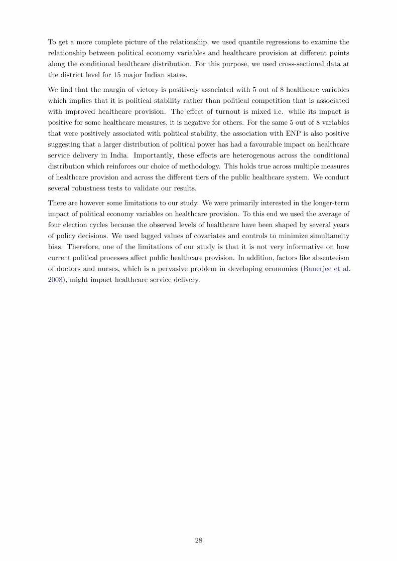
To get a more complete picture of the relationship, we used quantile regressions to examine the
relationship between political economy variables and healthcare provision at different points
along the conditional healthcare distribution. For this purpose, we used cross-sectional data at
the district level for 15 major Indian states.
We find that the margin of victory is positively associated with 5 out of 8 healthcare variables
which implies that it is political stability rather than political competition that is associated
with improved healthcare provision. The effect of turnout is mixed i.e. while its impact is
positive for some healthcare measures, it is negative for others. For the same 5 out of 8 variables
that were positively associated with political stability, the association with ENP is also positive
suggesting that a larger distribution of political power has had a favourable impact on healthcare
service delivery in India. Importantly, these effects are heterogenous across the conditional
distribution which reinforces our choice of methodology. This holds true across multiple measures
of healthcare provision and across the different tiers of the public healthcare system. We conduct
several robustness tests to validate our results.
There are however some limitations to our study. We were primarily interested in the longer-term
impact of political economy variables on healthcare provision. To this end we used the average of
four election cycles because the observed levels of healthcare have been shaped by several years
of policy decisions. We used lagged values of covariates and controls to minimize simultaneity
bias. Therefore, one of the limitations of our study is that it is not very informative on how
current political processes affect public healthcare provision. In addition, factors like absenteeism
of doctors and nurses, which is a pervasive problem in developing economies (Banerjee et al.
2008), might impact healthcare service delivery.
28

Appendices
A Matching constituencies to districts
Matching constituencies to their respective districts is a time-consuming task. This is further
complicated by redistrictings i.e. the process of redrawing district boundaries which often involve
carving out new districts from a single district or a combination of districts. For instance, there
were 466 districts in the 1991 census which increased to 593 during the 2001 census.
We first converted the data which we obtained from the ELection Commission of India into
machine readable format. We then matched individual constituencies to their respective districts
using the following algorithm: First, we obtained election results from the year 2004-05 which
includes matched district-constituency information. This was possible because the Delimitation
Order, 2003 did not come into effect until 2008. This was then modified to reflect the 2001
district boundaries, i.e. if a new district had been carved out after 2001 census, it was merged
back with its parent and all constituencies transferred. However, districts carved out of multiple
parents were dropped from the analysis. Those constituencies that remained unmatched at
the end of the first step were attempted to be matched using the matching scheme available
with www.empoweringindia.org, a non-profit organization that provides reliable information on
Indian elections on their website. And finally, constituencies without a matched district at the
end of the second step were matched using electoral orders from the Election Commission of India.
Once constituencies were matched to their respective districts, we aggregated constituency-level
data to the district-level which is used in our analysis.
B Normality and heteroscedasticity tests
B.1 Tests on OLS residuals
Table 10: Normality and heteroscedasticity
tests a b
W pW H pH
WV-HSC 0.986 0.000 217.5 0.000WV-PHC 0.884 0.000 328.1 0.000HSC-SLR 0.987 0.001 145.3 0.385PHC-SLR 0.986 0.000 248.2 0.000CHC-Ambulance 0.971 0.000 161.5 0.114HSC-ANM-SBA 0.980 0.000 227.4 0.000PHC-FMO 0.966 0.000 247.2 0.000CHC-GS 0.948 0.000 195.2 0.002a Shapiro-Wilk’s test for normality of OLS residuals.b White’s test for heteroscedasticity of OLS residuals.
29

B.2 Machado and Santos Silva (2000) heteroscedasticity test
Table 11: MSS Quantile heteroscedasticity testa
Variable q10 q25 q50 q75 q90
χ2 P-val χ2 P-val χ2 P-val χ2 P-val χ2 P-val
WV-HSC 8.29 0.02 32.98 0.00 58.00 0.00 47.79 0.00 44.84 0.00WV-PHC 50.32 0.00 51.31 0.00 70.46 0.00 145.64 0.00 216.61 0.00HSC-SLR 19.12 0.00 10.78 0.01 10.29 0.01 24.12 0.00 27.78 0.00PHC-SLR 41.71 0.00 62.09 0.00 66.95 0.00 34.84 0.00 49.62 0.00CHC-Ambulance 8.11 0.02 4.00 0.14 4.53 0.10 5.10 0.08 29.37 0.00HSC-ANM-SBA 2.48 0.29 15.83 0.00 70.57 0.00 41.72 0.00 17.57 0.00PHC-FMO 19.17 0.00 17.75 0.00 32.97 0.00 33.02 0.00 78.54 0.00CHC-GS 17.17 0.00 4.87 0.09 4.07 0.13 4.51 0.11 27.09 0.00a χ2 test results and corresponding p-values from Machado and Santos Silva (2000) quantile heteroscedasticity test.
C Construction of healthcare indices
Table 12: Percentage of total variance explained by PC1.
Indices(λi/
∑mi λi
)∗ 100
Public Health access:Overall Access 65.08Health Centre Access 80.00
Infrastructure:HSC 53.06PHC 36.47CHC 27.27
Human resource:HSC 53.48PHC 45.78CHC 37.83
Notes and sources:a Column 2 shows percentage of variance ex-
plained by PC1 i.e. the ratio of the eigenvaluecorresponding to PC1 to the sum of eigenvaluesof all the components.Data source: DLHS-3, 2007-08.
30

Table 13: Input variables used in creating health indicators
Indices Input variables
Public health access:
Broad access indexICDS(0.19), HSC(0.40), PHC(0.48), Block PHC(0.45), gov.dispensaries(0.42), AYUSH(0.45).
Only HSC/PHC/CHC HSC(0.55), PHC(0.62), CHC(0.56)
Infrastructure:
HSCLocated in government building(0.49), communication facility(0.37),separate labour room(0.50), ANM staying in HSC village(-0.19), staffquarter for ANM(0.57), regular water supply(0.11).
PHC
Residential quarter MO(0.21), separate labour room(0.42), personalcomputer(0.25), normal delivery kit(0.41), large deep freezer(0.39),regular water supply(0.18), neonatal warmer(0.28), OT with Boyle’sapparatus(0.35), OT with anaesthetic medicine(0.35), plan for currentyear(0.21).
CHCPersonal computer (0.14), operation theatre(0.53), labour room(0.58),blood storage facility(0.16), large deep freezer(0.32), plan for currentyear(0.12), 24-hr water supply(0.46), ambulance on road(-0.05)
Human resource:
HSCMale health worker in position(0.23), ANM had: ISD training in last 5years(0.42), ever been trained in ISD(0.39), IMNCI in last 5 years(0.48),ever been trained in IMNCI(0.46), ANM attended SBA training(0.40).
PHCLady MO(0.56), lab technician (0.52), org. training prog. lastyear(-0.14), at least one MO attended: ISD training (12d in last 5years) (0.25), IMNCI (in last 5 years)(0.58).
CHCGeneral surgeon (0.41), Obst./Gyn(0.45), MO training in last 5 years:NSV(0.43), HIV/AIDS(0.15), Basic emergency/Obst. care(0.51),Neo-natal care(0.39)
Notes and sources:
The extracted weights from the first principal component are in parenthesis.The abbreviations used in the table are as follows: ICDS - Integrated Childhood Development Services;HSC - Health Sub-Centre; PHC - Primary Healthcare Centre; AYUSH - Ayurveda, Yoga, Unani, Siddhaand Homeopathy; MO - Medical Officer; HIV/AIDS - Human Immunodeficiency Virus/ Acquired ImmuneDeficiency Syndrome; Obst.- Obstetrician; Gyn.- Gynecologist; NSV - Non-Scalpel Vasectomy; IMNCI -Integrated Management of Neo-natal and Childhood Illnesses; ICTC - Integrated Counselling and TestingCentre for HIV; OT - Operation Theatre; ISD - Integrated Skill Development Training; ANM - AuxiliaryNurse/ Midwife; SBA - Skilled Birth Attendant.Data source: DLHS-3, 2007-08.
31

References
Aidt, T., Dutta, J. and Loukoianova, E. (2006), ‘Democracy comes to Europe: Franchise
extension and fiscal outcomes 1830 – 1938 ’, European Economic Review 50(2), 249 – 283.
Aidt, T. S., Daunton, M. and Dutta, J. (2010), ‘The Retrenchment Hypothesis and the Extension
of the Franchise in England and Wales’, The Economic Journal 120(547), 990–1020.
Aidt, T. S. and Eterovic, D. S. (2011), ‘Political competition, electoral participation and public
finance in 20th century Latin America’, European Journal of Political Economy 27(1), 181 –
200.
Aldrich, J. H. (1993), ‘Rational choice and turnout’, American Journal of Political Science
37(1), 246–278.
Alesina, A., Baqir, R. and Easterly, W. (1999), ‘Public goods and ethnic divisions’, The Quarterly
Journal of Economics 114(4), 1243–1284.
Alesina, A. and La Ferrara, E. (2000), ‘Participation in heterogeneous communities’, The
Quarterly Journal of Economics 115(3), 847–904.
Arrow, K. J. (1963), ‘Uncertainty and the welfare economics of medical care’, The American
economic review 53(5), 941–973.
Banerjee, A. V., Duflo, E. and Glennerster, R. (2008), ‘Putting a band-aid on a corpse: Incentives
for nurses in the indian health care system.’, Journal of the European Economic Association
6(2/3), 487 – 500.
Baskaran, T., Min, B. and Uppal, Y. (2015), ‘Election cycles and electricity provision: Evidence
from a quasi-experiment with indian special elections’, Journal of Public Economics 126, 64 –
73.
Betancourt, R. and Gleason, S. (2000), ‘The Allocation of Publicly-Provided Goods to Rural
Households in India: On Some Consequences of Caste, Religion and Democracy’, World
Development 28(12), 2169–2182.
Blomquist, S. and Christiansen, V. (1999), ‘The political economy of publicly provided private
goods’, Journal of Public Economics 73(1), 31–54.
Buchanan, J. M. and Tullock, G. (1962), ‘The calculus of consent: Logical foundations of
constitutional democracy (ann arbor paperbacks)’.
Cade, B. S. and Noon, B. R. (2003), ‘A gentle introduction to quantile regression for ecologists’,
Frontiers in Ecology and the Environment 1(8), 412–420.
Collier, P. (2000), ‘Ethnicity, politics and economic performance’, Economics & Politics
12(3), 225–245.
Crost, B. and Kambhampati, U. S. (2010), ‘Political Market Characteristics and the Provision
of Educational Infrastructure in North India’, World Development 38(2), 195–204.
Downs, A. (1957), An Economic Theory of Democracy, Harper.
32
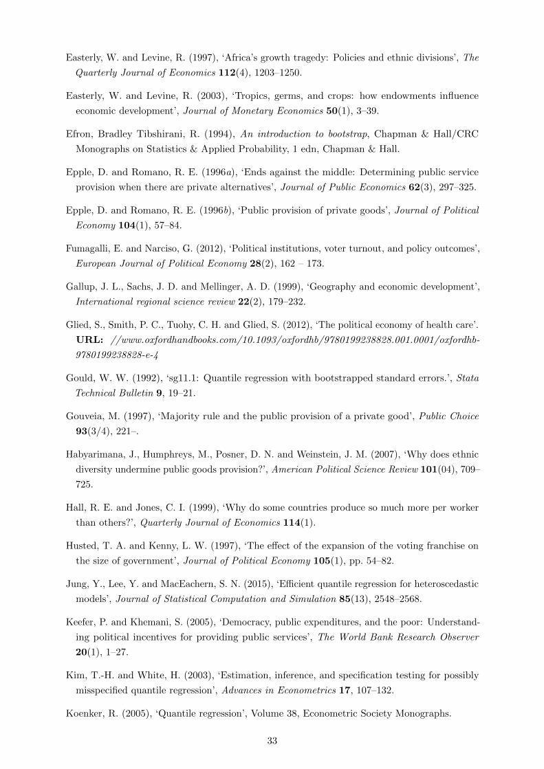
Easterly, W. and Levine, R. (1997), ‘Africa’s growth tragedy: Policies and ethnic divisions’, The
Quarterly Journal of Economics 112(4), 1203–1250.
Easterly, W. and Levine, R. (2003), ‘Tropics, germs, and crops: how endowments influence
economic development’, Journal of Monetary Economics 50(1), 3–39.
Efron, Bradley Tibshirani, R. (1994), An introduction to bootstrap, Chapman & Hall/CRC
Monographs on Statistics & Applied Probability, 1 edn, Chapman & Hall.
Epple, D. and Romano, R. E. (1996a), ‘Ends against the middle: Determining public service
provision when there are private alternatives’, Journal of Public Economics 62(3), 297–325.
Epple, D. and Romano, R. E. (1996b), ‘Public provision of private goods’, Journal of Political
Economy 104(1), 57–84.
Fumagalli, E. and Narciso, G. (2012), ‘Political institutions, voter turnout, and policy outcomes’,
European Journal of Political Economy 28(2), 162 – 173.
Gallup, J. L., Sachs, J. D. and Mellinger, A. D. (1999), ‘Geography and economic development’,
International regional science review 22(2), 179–232.
Glied, S., Smith, P. C., Tuohy, C. H. and Glied, S. (2012), ‘The political economy of health care’.
URL: //www.oxfordhandbooks.com/10.1093/oxfordhb/9780199238828.001.0001/oxfordhb-
9780199238828-e-4
Gould, W. W. (1992), ‘sg11.1: Quantile regression with bootstrapped standard errors.’, Stata
Technical Bulletin 9, 19–21.
Gouveia, M. (1997), ‘Majority rule and the public provision of a private good’, Public Choice
93(3/4), 221–.
Habyarimana, J., Humphreys, M., Posner, D. N. and Weinstein, J. M. (2007), ‘Why does ethnic
diversity undermine public goods provision?’, American Political Science Review 101(04), 709–
725.
Hall, R. E. and Jones, C. I. (1999), ‘Why do some countries produce so much more per worker
than others?’, Quarterly Journal of Economics 114(1).
Husted, T. A. and Kenny, L. W. (1997), ‘The effect of the expansion of the voting franchise on
the size of government’, Journal of Political Economy 105(1), pp. 54–82.
Jung, Y., Lee, Y. and MacEachern, S. N. (2015), ‘Efficient quantile regression for heteroscedastic
models’, Journal of Statistical Computation and Simulation 85(13), 2548–2568.
Keefer, P. and Khemani, S. (2005), ‘Democracy, public expenditures, and the poor: Understand-
ing political incentives for providing public services’, The World Bank Research Observer
20(1), 1–27.
Kim, T.-H. and White, H. (2003), ‘Estimation, inference, and specification testing for possibly
misspecified quantile regression’, Advances in Econometrics 17, 107–132.
Koenker, R. (2005), ‘Quantile regression’, Volume 38, Econometric Society Monographs.
33

Koenker, R. and Bassett, Gilbert, J. (1978), ‘Regression quantiles’, Econometrica 46(1), 33–50.
Koenker, R. and Hallock, K. F. (2001), ‘Quantile Regression’, Journal of Economic Perspectives
15(4), 143–156.
Kremer, M. and Glennerster, R. (2011), Chapter four - improving health in developing countries:
Evidence from randomized evaluations1, in T. G. M. Mark V. Pauly and P. P. Barros, eds,
‘Handbook of Health Economics’, Vol. 2 of Handbook of Health Economics, Elsevier, pp. 201 –
315.
Laakso, M. and Taagepera, R. (1979), ‘The” effective” number of parties:” a measure with
application to west europe”’, Comparative political studies 12(1), 3.
Lutz, G. and Marsh, M. (2007), ‘Introduction: Consequences of low turnout’, Electoral Studies
26(3), 539 – 547.
Machado, J. A. and Silva, J. (2013), ‘Quantile regression and heteroskedasticity’, Discussion
Paper, University of Essex, Department of Economics .
Machado, J. A. and Silva, J. S. (2000), ‘Glejser’s test revisited’, Journal of Econometrics
97(1), 189–202.
Mani, A. and Mukand, S. (2007), ‘Democracy, Visibility and Public Good Provision’, Journal of
Development Economics 83(2), 506–529.
Meltzer, A. H. and Richard, S. F. (1981), ‘A Rational Theory of the Size of Government’, Journal
of Political Economy 89(5), 914–927.
Miguel, E. and Gugerty, M. (2005), ‘Ethnic diversity, social sanctions, and public goods in
Kenya’, Journal of Public Economics 89(11-12), 2325–2368.
Mobarak, A. M., Rajkumar, A. S. and Cropper, M. (2011), ‘The political economy of health
services provision in brazil’, Economic Development and Cultural Change 59(4), 723–751.
Mueller, D. C. and Stratmann, T. (2003), ‘The economic effects of democratic participation’,
Journal of Public Economics 87(910), 2129 – 2155.
Neto, O. A. and Cox, G. W. (1997), ‘Electoral institutions, cleavage structures, and the number
of parties’, American Journal of Political Science pp. 149–174.
Powell, J. L. (1994), ‘Estimation of semiparametric models’, Handbook of Econometrics 4, 2443–
2521.
Roberts, K. W. (1977), ‘Voting over income tax schedules’, Journal of Public Economics 8(3), 329
– 340.
Robinson, J. A. and Torvik, R. (2005), ‘White elephants’, Journal of Public Economics 89(2), 197–
210.
Spolaore, E. and Wacziarg, R. (2013), ‘How deep are the roots of economic development?’,
Journal of Economic Literature 51(2), 325–369.
34

van Doorslaer, E., O’Donnell, O., Rannan-Eliya, R. P., Somanathan, A., Adhikari, S. R., Garg,
C. C., Harbianto, D., Herrin, A. N., Huq, M. N., Ibragimova, S., Karan, A., Ng, C. W., Pande,
B. R., Racelis, R., Tao, S., Tin, K., Tisayaticom, K., Trisnantoro, L., Vasavid, C. and Zhao,
Y. (2006), ‘Effect of payments for health care on poverty estimates in 11 countries in asia: an
analysis of household survey data’, The Lancet 368(9544), 1357 – 1364.
Varshney, A. (2000), ‘Is India Becoming More Democratic?’, The Journal of Asian Studies
59(1), pp. 3–25.
35


![Smart[er] Smart Urban Safety & Security| Surveillance| Crime Prevention| Conflict Mediation| Healthcare Provision](https://cdn.vdocument.in/doc/165x107/56649e6b5503460f94b6a1e5/smarter-smart-urban-safety-security-surveillance-crime-prevention-conflict.jpg)


