
PRACTICE!
The use the WEKA software. It is opensource (GNU) freely downloadable from
http://www.cs.waikato.ac.nz/ml/weka/ Weka 3.6 is the latest stable version of Weka. Weka is a collection of algorithms for data mining
tasks and contains tools for data pre-processing, classification, regression, clustering, association rules, and visualization.
Tutorials can be found at the Weka web site
1
Data M
inin
g Cou
rse - UF
PE
- Jun
e 2012
MACHINE LEARNING WITH WEKA
Comprehensive set of tools: Pre-processing and data analysis Mining algorithms
(for classification, clustering, etc.) Evaluation metrics
Three modes of operation: GUI command-line (not discussed) Java API (not discussed) Weka can read ARFF file or CSV files.
2
Data M
inin
g Cou
rse - UF
PE
- Jun
e 2012
ARFF FILES
ARFF files have two distinct sections. Header information: The Header of the ARFF file
contains the name of the relation, a list of the attributes (the columns in the data), and their types.
Data information.
3
Data M
inin
g Cou
rse - UF
PE
- Jun
e 2012
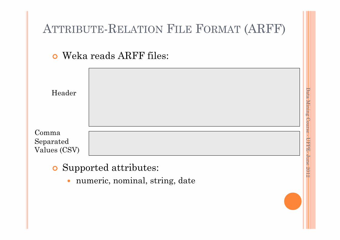
ATTRIBUTE-RELATION FILE FORMAT (ARFF)
Weka reads ARFF files:
@relation adult @attribute age numeric @attribute name string @attribute education {College, Masters, Doctorate} @attribute class {>50K,<=50K} @data
50,Leslie,Masters,>50K ?,Morgan,College,<=50K
Supported attributes: numeric, nominal, string, date
4
Comma Separated Values (CSV)
Header
Data M
inin
g Cou
rse - UF
PE
- Jun
e 2012
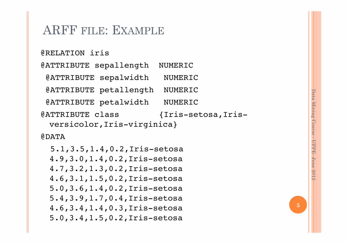
ARFF FILE: EXAMPLE
@RELATION iris !
@ATTRIBUTE sepallength NUMERIC !
@ATTRIBUTE sepalwidth NUMERIC !
@ATTRIBUTE petallength NUMERIC !
@ATTRIBUTE petalwidth NUMERIC !
@ATTRIBUTE class {Iris-setosa,Iris-versicolor,Iris-virginica} !
@DATA !
5.1,3.5,1.4,0.2,Iris-setosa 4.9,3.0,1.4,0.2,Iris-setosa 4.7,3.2,1.3,0.2,Iris-setosa 4.6,3.1,1.5,0.2,Iris-setosa 5.0,3.6,1.4,0.2,Iris-setosa 5.4,3.9,1.7,0.4,Iris-setosa 4.6,3.4,1.4,0.3,Iris-setosa 5.0,3.4,1.5,0.2,Iris-setosa
5
Data M
inin
g Cou
rse - UF
PE
- Jun
e 2012
DATA MINING PRACTICE: EXPLORING DATA
6
Data M
inin
g Cou
rse - UF
PE
- Jun
e 2012
WHAT IS DATA EXPLORATION?
Key motivations of data exploration include Helping to select the right tool for preprocessing or analysis Making use of humans’ abilities to recognize patterns
People can recognize patterns not captured by data analysis tools
Related to the area of Exploratory Data Analysis (EDA)
A preliminary exploration of the data to better understand its characteristics.
VISUALIZATION
Visualization is the conversion of data into a visual or tabular format so that the characteristics of the data and the relationships among data items or attributes can be analyzed or reported.
Visualization of data is one of the most powerful and appealing techniques for data exploration. Humans have a well developed ability to analyze large
amounts of information that is presented visually Can detect general patterns and trends Can detect outliers and unusual patterns
8
Data M
inin
g Cou
rse - UF
PE
- Jun
e 2012
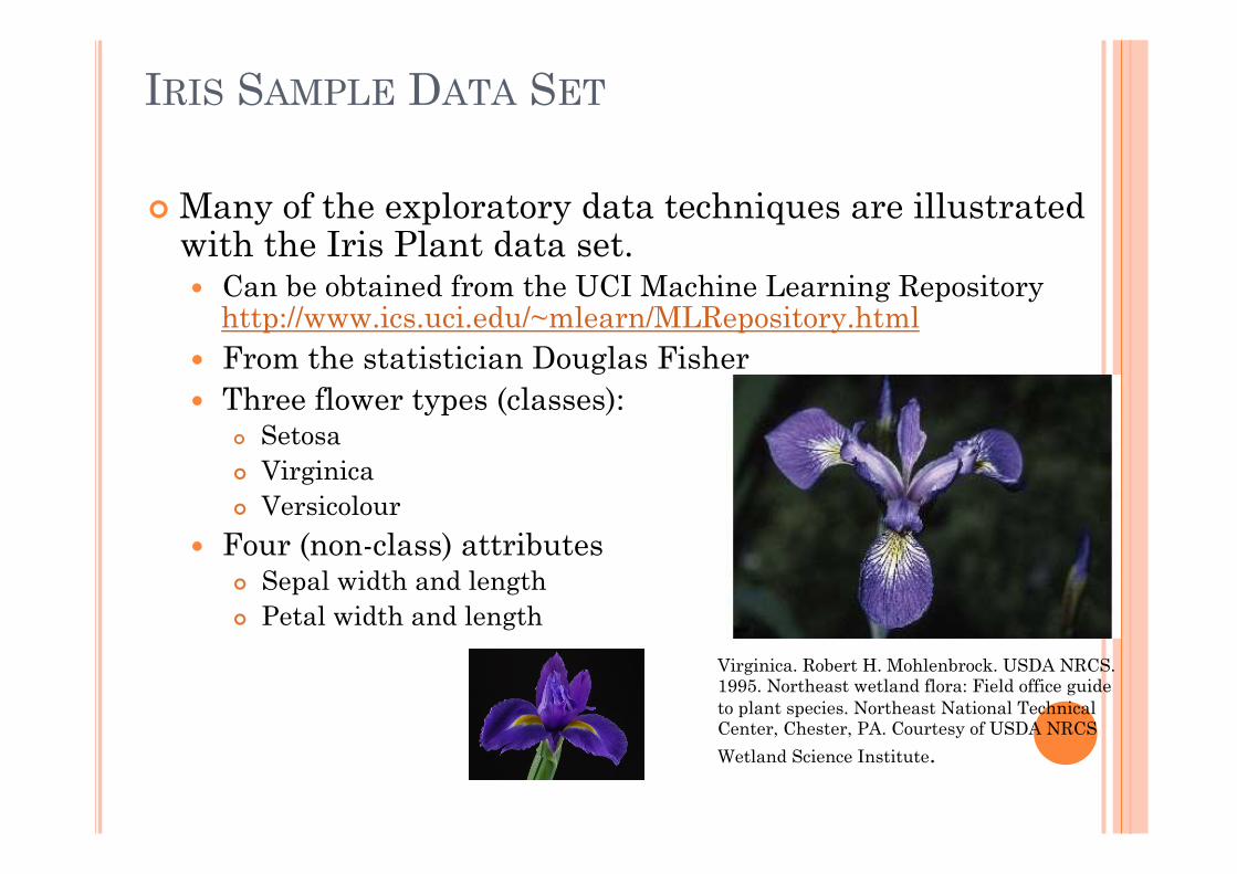
IRIS SAMPLE DATA SET
Many of the exploratory data techniques are illustrated with the Iris Plant data set. Can be obtained from the UCI Machine Learning Repository
http://www.ics.uci.edu/~mlearn/MLRepository.html From the statistician Douglas Fisher Three flower types (classes):
Setosa Virginica Versicolour
Four (non-class) attributes Sepal width and length Petal width and length
Virginica. Robert H. Mohlenbrock. USDA NRCS. 1995. Northeast wetland flora: Field office guide to plant species. Northeast National Technical Center, Chester, PA. Courtesy of USDA NRCS
Wetland Science Institute.
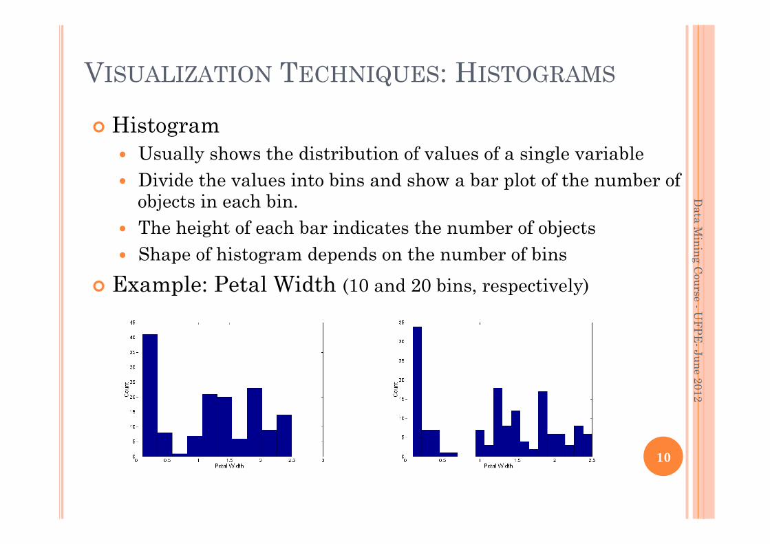
VISUALIZATION TECHNIQUES: HISTOGRAMS
Histogram Usually shows the distribution of values of a single variable Divide the values into bins and show a bar plot of the number of
objects in each bin. The height of each bar indicates the number of objects Shape of histogram depends on the number of bins
Example: Petal Width (10 and 20 bins, respectively)
10
Data M
inin
g Cou
rse - UF
PE
- Jun
e 2012
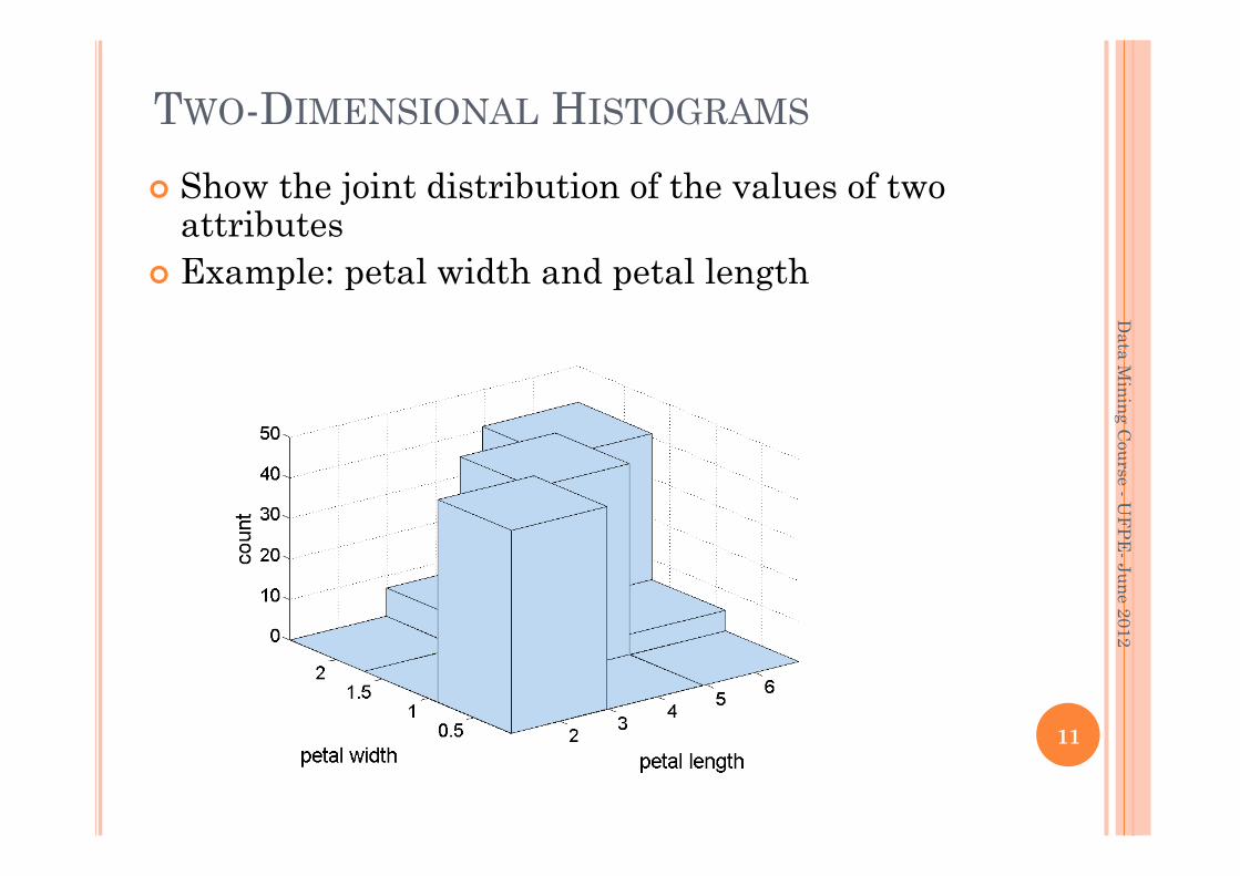
TWO-DIMENSIONAL HISTOGRAMS
Show the joint distribution of the values of two attributes
Example: petal width and petal length
11
Data M
inin
g Cou
rse - UF
PE
- Jun
e 2012
VISUALIZATION TECHNIQUES: SCATTER PLOTS
Scatter plots Attributes values determine the position Two-dimensional scatter plots most common, but can have
three-dimensional scatter plots Often additional attributes can be displayed by using the
size, shape, and color of the markers that represent the objects
It is useful to have arrays of scatter plots can compactly summarize the relationships of several pairs of attributes See example on the next slide
12
Data M
inin
g Cou
rse - UF
PE
- Jun
e 2012
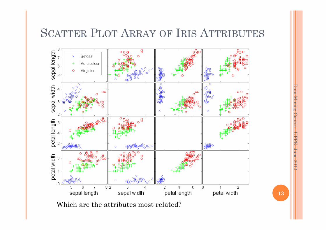
SCATTER PLOT ARRAY OF IRIS ATTRIBUTES
Which are the attributes most related?
13
Data M
inin
g Cou
rse - UF
PE
- Jun
e 2012

PRACTICE!
Data M
inin
g Cou
rse - UF
PE
- Jun
e 2012
14
DATA PREPROCESSING: EXERCISE 1
Download and install the last stable version of Weka
Open Weka, select the Explorer button and load the IRIS dataset How many records are in this dataset? How many attributes? And classes? Which are the types of the attribute? Which is the attribute with greatest standard
deviation? Which is the interpretation of this value? Visualize the plot of all the attributes. Which are the
most correlated? 15
Data M
inin
g Cou
rse - UF
PE
- Jun
e 2012
DATA PREPROCESSING: EXERCISE 2
Preprocessing on the Iris dataset: Discretize the numeric attributes of the Iris
dataset using the unsupervised Discretize filter into 5 bins.
Notice the obtained discretization. How many elements in each interval? Is this discretization well balanced?
Now “undo” and try supervised discretization: how many bins you have now? Are the intervals well balanced?
Which are the attributes most relevant respect to the class?
16
Data M
inin
g Cou
rse - UF
PE
- Jun
e 2012
DATA PREPROCESSING: EXERCISE 3
Load the dataset old_faithful Use the visualization tab to perform visual
inspection Visualize the scatter plot for the combinations of:
F1 vs F2. Are these attributes related or not? Determine visually the data points that are the
outliers (extreme high or low values). From the preprocessing tab, normalize the
attributes to be in the [0,1] interval – use of the Normalize filter
17
Data M
inin
g Cou
rse - UF
PE
- Jun
e 2012
DATA PREPROCESSING: EXERCISE 4
Load the breast cancer dataset CSV version How is the attribute values distribution? Remove the ID using the Remove filter How is the correlation between the variables?
18
Data M
inin
g Cou
rse - UF
PE
- Jun
e 2012
DATA PREPROCESSING: EXERCISE 5
Prepare data for Weka: read the car dataset information and edit the car dataset to be read by Weka.
Remind you need the CSV format, therefore the name of the attributes must appear in the first row. You can use Excel or a text editor.
19
Data M
inin
g Cou
rse - UF
PE
- Jun
e 2012
PREPROCESSING: EXERCISE 6
Load the bank dataset. Edit data to make some missing values: Delete some data in “region”(Nominal) and
“children”(Numeric) attributes. Click on “OK” button when finish Choose “ReplaceMissingValues” filter Look into the data. How did those missing values
get replaced ? Save the file as bank-data-missing.arff
20
Data M
inin
g Cou
rse - UF
PE
- Jun
e 2012
CLASSIFICATION: EXERCISE 1
Load in Weka the Weather dataset and select the Classify tab
Select the classifier J48 and run with the default options.
Visualize the tree Visualize the errors Play with the parameters of J48 to improve the
quality of the classifier
Data M
ining Course - U
FPE- June 2012
21
CLASSIFICATION: EXERCISE 2
Load the Bank dataset Run J48 with default values. How is the
performance of the tree? Try to apply feature selection to improve the
performance. Try Cross-validation 10 folds / Use training set /
Percentage split. Which is the best? Play with parameters to improve the
performance. Which is the best combination?
Data M
ining Course - U
FPE- June 2012
22
CLASSIFICATION: EXERCISE 3 Load the Breast cancer dataset Run some of the classifiers available on weka (recall
that decision tree needs discretized values…) with different options and to find the best result
Which is the best classification and how many instances are incorrectly classified?
What can you infer from the information shown in the Confusion Matrix?
Visualize the classifier errors. In the plot, how can you differentiate between the correctly and incorrectly classified instances? In the plot, how can you see the detailed information of an incorrectly classified instance?
Save the learned classifier to a file How can you load a learned classifier from a file?
Data M
ining Course - U
FPE- June 2012
23
CLASSIFICATION: EXERCISE 4
Load the zoo dataset Go to the classifier tab and select the decision
tree classifier j48 Which percentage of instances is correctly
classified by j48? Which families are mistaken for each other? Change to binarySplit and build a new decision
tree. What is the difference? Experiment with some of the other classifiers and
until you get a better classification performance. Write down the classifier and its performance.
Data M
ining Course - U
FPE- June 2012
24
CLASSIFICATION: EXERCISE 5
Load the ’labour’ data set (labor.arff) that contains data of acceptable and unacceptable labour contracts.
Examine the data and attributes and make sure you understand their meaning.
Run J48 with all options set to default. Make sure that the class attribute is selected as the classification label, and that you have selected cross-validation. Right click on the experiment (left panel – the Result list) and select the Visualize tree option.
Analyse the the resulting accuracy. Analyse the detailed accuracy by classes – what are TP and FP? Make sure you understand all the data reported in the classifier output pane (e.g. confusion matrix)? Which class is easier to predict?
Repeat the classification using the vacation attribute as the classification label. Are these results acceptable?
25
Data M
inin
g Cou
rse - UF
PE
- Jun
e 2012
CLUSTERING: EXERCISE 1
Load the Iris dataset Visualize the dataset from the Visualize tab. Now select the cluster tab, the “use training set”
option and run the algorithms cobweb and SimpleKmeans.
Right click each of the results and visualize the cluster assignments
Compare the cluster assignment with the class labeled plot
Which cluster is the best?
26
Data M
inin
g Cou
rse - UF
PE
- Jun
e 2012
CLUSTERING: EXERCISE 2
Now run again the algorithms but select the option “classes to cluster evaluation”. In this mode Weka ignores the class attribute and generates the clustering. Then it compares the obtained cluster with the classes to compute the classification error.
Which cluster is the best? Play with cluster options to improve clustering
results.
27
Data M
inin
g Cou
rse - UF
PE
- Jun
e 2012
CLUSTERING: EXERCISE 3
With the IRIS dataset loaded, remove the class attribute with the preprocessing tab.
Then run the DBScan algorithm. How many clusters did it find? Change the parameters setting to improve the
result
28
Data M
inin
g Cou
rse - UF
PE
- Jun
e 2012
CLUSTERING: EXERCISE 4
Load the Bank dataset Run the simpleKMeans setting 6 clusters Which are centroids of the cluster? How can you
characterize each cluster? Now visualize the clusters graphically. You can
choose the cluster number and any of the other attributes for each of the three different dimensions available. Explore the discovered cluster.
Now change the cluster parameters. How the cluster changes?
Try the ignore attribute option. Which is the best clustering?
Save the best clustering you find
29
Data M
inin
g Cou
rse - UF
PE
- Jun
e 2012

CLUSTERING: EXERCISE 5
Load the flag dataset Run the coweb clustering algorithm (hierarchical)
with parameters A=1.0 and C=0.4 Visualize the cluster output. Change the parameters and visualize the results. How can you interpret the output? Try the “classes to cluster evaluation ”option.
How good is the resulting clustering?
30
Data M
inin
g Cou
rse - UF
PE
- Jun
e 2012
ASSOCIATION RULES: EXERCISE 1
Load the bank dataset and discretize the attributes that are numeric. This pre-processing can be done with filtering.
Now run the association rule algorithm and play with the parameters.
Which rules are always true? Write them down. Write down a couple of interesting rules and a
couple of trivial rules.
31
Data M
inin
g Cou
rse - UF
PE
- Jun
e 2012
ASSOCIATION RULES: EXERCISE 2
Load Iris dataset and run association analysis (note that association rules work on nominal attributes!)
generate 10 association rules and discuss some inferences you would make from them
Then change the support and confidence to lower values. What happened?
Select the OutputItemset option and run again the Apriori algorithm. What’s happened?
32
Data M
inin
g Cou
rse - UF
PE
- Jun
e 2012
ASSOCIATION RULES: EXERCISE 3
Load the contact-lens dataset and run association analysis Apriori
Which is the best rule found? Can you correlate this rule with the decision
tree?
33
Data M
inin
g Cou
rse - UF
PE
- Jun
e 2012
ASSOCIATION RULES: EXERCISE 4
Load the Weather-nominal dataset
Run association analysis. How many rules fund? Which is the maximum support for which you can
find rules? Try to adjust the confidence to find rules with higher support. What is the interpretation?
34
Data M
inin
g Cou
rse - UF
PE
- Jun
e 2012
ASSOCIATION RULES: EXERCISE 5 Load the zoo dataset Deselect the animal and legs attributes. The animal attribute is the
name of the animal, and is not useful for mining. The legs attribute is numeric and cannot be used directly with Apriori.
Alternatively, you can try to use the Discretize Filter to discretize the legs attribute.
Try Apriori algorithm with the default parameters. Record the generated rules.
Vary the number of rules generated. Try 20, 30, ... Record how many rules you have to generate before generating a rule containing type=mammal.
Vary the maximum support until a rule containing type=mammal is the top rule generated. Record the maximum support needed.
Select one generated rule that was interesting to you. Why was it interesting? What does it mean? Check its confidence and
support – are they high enough?
35
Data M
inin
g Cou
rse - UF
PE
- Jun
e 2012


