

PRATIBHA: INTERNATIONAL JOURNAL OF
SCIENCE, SPIRITUALITY, BUSINESS AND
TECHNOLOGY
(IJSSBT)
Vol.1, No.2, February 2013
ISSN (Print) : 2277-7261
ISSN (on-line) : 2278-3857
EDITOR(s)-IN-CHIEF:
Prof. Dr. Kishor S. Wani
Prof. Dr. Dheeraj Sheshrao Deshmukh
IJSSBT

PRATIBHA: INTERNATIONAL JOURNAL OF SCIENCE,
SPIRITUALITY, BUSINESS AND TECHNOLOGY (IJSSBT)
Pratibha: International Journal of Science, Spirituality, Business And Technology
(IJSSBT) is a research journal published by Shram Sadhana Bombay Trust‘s, COLLEGE Of
ENGINEERING & TECHNOLOGY, Bambhori, Jalgaon, MAHARASHTRA STATE, INDIA. College was
founded by FORMER PRESIDENT, GOVT. OF INDIA, Honorable Excellency
Sau. PRATIBHA DEVI SINGH PATIL.
College is awarded as Best Engineering College of Maharashtra State by
Engineering Education Foundation, Pune in year 2008-09.
The College has ten full-fledged departments. The Under Graduate programs in 7
courses are accredited by National Board of Accreditation, All India Council for
Technical Education, New Delhi for 5 years with effect from 19/07/2008 vide letter
number NBA/ACCR-414/2004. QMS of the College conforms to ISO 9001:2008 and is
certified by JAAZ under the certificate number: 1017-QMS-0117.The college has been
included in the list of colleges prepared under Section 2(f) of the UGC Act, 1956 vide
letter number F 8-40/2008 (CPP-I) dated May, 2008 and 12(B) vide letter number F. No.
8-40/2008(CPP-I/C) dated September 2010. UG courses permanently affiliated to North
Maharashtra University are: Civil Engineering, Chemical Engineering, Computer
Engineering, Electronics and Telecommunication Engineering, Electrical Engineering,
Mechanical Engineering, Information Technology. Two years Post Graduate courses are
Mechanical Engineering (Machine Design), Civil Engineering (Environmental
Engineering), Computer Engineering (Computer Science and Engineering), Electronics
and Telecommunication (Digital Electronics). Civil Engineering Department,
Mechanical, Biotechnology and Chemical Engineering Department laboratories are
registered for Ph.D. Programs. Spread over 25 Acres, the campus of the college is
beautifully located on the bank of River Girna.
The International Journal of Science, Spirituality, Business and Technology
(IJSSBT) is an excellent, intellectual, peer reviewed journal that takes scholarly approach
in creating, developing, integrating, sharing and applying knowledge about all the fields
of study in Engineering, Spirituality, Management and Science for the benefit of
humanity and the profession.
The audience includes researchers, managers, engineers, curriculum designers
administrators as well as developers.

AIM AND SCOPE
Our philosophy is to map new frontiers in emerging and developing technology areas in research, industry and governance, and to link with centers of excellence worldwide to provide
authoritative coverage and references in focused and specialised fields. The journal presents its
readers with broad coverage across all branches of Engineering, Management, Spirituality and
Science of the latest development and their applications.
All technical, research papers and research results submitted to IJSSBT should be original in
nature. Contributions should be written for one of the following categories:
1. Original research
2. Research Review / Systematic Literature Review
3. Short Articles on ongoing research 4. Preliminary Findings
5. Technical Reports / Notes
IJSSBT publishes on the following topics but NOT LIMITED TO:
SCIENCES
Computational and industrial
mathematics and statistics, and other
related areas of mathematical sciences Approximation theory
Computation
Systems control Differential equations and dynamical
systems
Financial math Fluid mechanics and solid mechanics
Functional calculus and applications
Linear and nonlinear waves
Numerical algorithms Numerical analysis
Operations research
Optimization Probability and stochastic processes
Simulation
Statistics Wavelets and wavelet transforms
Inverse problems
Artificial intelligence
Neural processing
Nuclear and particle physics Geophysics
Physics in medicine and biology
Plasma physics Semiconductor science and
technology
Wireless and optical communications Materials science
Energy and fuels
Environmental science and
technology Combinatorial chemistry
Natural products
Molecular therapeutics Geochemistry
Cement and concrete research,
Metallurgy Crystallography and
Computer-aided materials design
COMPUTER ENGINEERING AND INFORMATION TECHNOLOGY
Information Systems e-Commerce Intelligent Systems
Information Technology
e-Government
Language and Search Engine Design Data Mining and Web Mining
Cloud Computing
Distributed Computing
Telecommunication Systems Artificial Intelligence
Virtual Business and Enterprise
Computer Systems
Computer Networks Database Systems and Theory
Knowledge Management

Computational Intelligence
Simulation and Modeling Scientific Computing and HPC
Embedded Systems
Control Systems
ELECTRONICS AND TELECOMMUNICATION ENGINEERING
3D Vision
3D TV
Biometrics Graph-based Methods
Image and video indexing and
database retrieval Image and video processing
Image-based modeling
Kernel methods
Model-based vision approaches Motion Analysis
Non-photorealistic animation and
modeling Object recognition
Performance evaluation
Segmentation and grouping Shape representation and analysis
Structural pattern recognition
Computer Graphics Systems and
Hardware Rendering Techniques and Global
Illumination
Real-Time Rendering Fast Algorithms
Fast Fourier Transforms
Digital Signal Processing
Wavelet Transforms Mobile Signal Processing
Statistical Signal Processing
Optical Signal Processing Data Mining Techniques
Motion Detection
Content-based Image retrieval Video Signal Processing
Watermarking
Signal Identification
Detection and Estimation of Signal Parameters
Nonlinear Signals and Systems
Signal Reconstruction
Time-Frequency Signal Analysis Filter Design and Structures
Spectral Analysis
Adaptive and Clustering Algorithms Fast Fourier Transforms
Virtual, Augmented and Mixed
Reality
Geometric Computing and Solid Modeling
Game Design and Engine
Development 3D Reconstruction
GPU Programming
Graphics and Multimedia Image Processing
Interactive Environments
Software and Web accessibility
Graphics & Perception Computational Photography
Pattern recognition and analysis
Medical image processing Visualization
Image coding and compression
Face Recognition
Image segmentation Radar Image Processing
Sonar Image Processing
Signal Identification Super-resolution imaging
Signal Reconstruction
Filter Design Adaptive Filters
Multi-channel Filtering
Noise Control
Control theory and practice
CIVIL ENGINEERING
Geotechnical Structures
Transportation
Environmental Engineering Earthquakes
Water Resources
Hydraulic and Hydraulic Structures
Construction Management, and Material
Structural mechanics
Soil mechanics and Foundation Engineering
Coastal engineering and River
engineering

Ocean Engineering
Fluid-solid-structure interactions, offshore engineering and marine
structures
Constructional management and other
civil engineering relevant areas Surveying
Transportation Engineering
CHEMICAL ENGINEERING
Organic Chemistry Inorganic Chemistry
Physical Chemistry
Analytical Chemistry Biological Chemistry
Industrial Chemistry
Agricultural & Soil Chemistry Petroleum Chemistry
Polymers Chemistry
Nanotechnology
Green Chemistry Forensic
Photochemistry
Computational Chemical Physics
Chemical Engineering
Wastewater treatment and engineering Biosorption
Chemisorptions
Heavy metal remediation
Phytoremediation Novel treatment processes for
wastewaters
Land reclamation methods Solid waste treatment
Anaerobic digestion
Gasification Landfill issues
Leachate treatment and gasification
Water and Wastewater Minimization Mass integration
Emission Targeting
Pollution Control
Safety and Loss Prevention Conceptual Design
Mathematical Approach
Pinch Technology Energy Audit
Production Technical Knowledge
Process Design Heat Transfer
Chemical Reaction Engineering
Modeling and simulation
Process Equipment Design
ELECTRICAL ENGINEERING
Power Engineering
Electrical Machines
Instrumentation and control
Electric Power Generation Transmission and Distribution
Power Electronics
Power Quality and Economic Renewable Energy
Electric Traction, Electromagnetic
Compatibility and Electrical
Engineering Materials
High Voltage Insulation Technologies High Voltage Apparatuses
Lightning Detection and Protection
Power System Analysis, SCADA and Electrical Measurements
MECHANICAL ENGINEERING
Fluid mechanics Heat transfer
Solid mechanics
Refrigeration and air conditioning
Renewable energy technology Materials engineering
Composite materials
Marine engineering Petroleum and mineral resources
engineering
Textile engineering Leather technology
Industrial engineering
Operational research
Manufacturing processes Machine design
Quality control
Mechanical maintenance Tribology

MANAGEMENT
Accounting and Finance
Marketing
Operations Management Human resource management
Management Strategy
Information technology
Business Economics
Public Sector management Organizational behavior
Research methods
SPIRITUALITY
Relevance of Science and Spirituality
in decision and Policy making
Rigors in Scientific Research and
Insights from Spiritual wisdom Dividends from Scientific research
and Spiritual Temper
Spiritual Wisdom in disaster
management
Techno-Spiritual aspects of
development
BIO-TECHNOLOGY
Molecular biology and the chemistry
of biological process to aquatic and
earth environmental aspects as well as computational applications
Policy and ethical issues directly
related to Biotechnology
Molecular biology Genetic engineering
Microbial biotechnology
Plant biotechnology
Animal biotechnology
Marine biotechnology Environmental biotechnology
Biological processes
Industrial applications
Bioinformatics Biochemistry of the living cell
Bioenergetics
IJSSBT prides itself in ensuring the high quality and professional standards.
All submitted papers are to be peer-reviewed for ensuring their qualities.
Frequency : Two issues per year
Page charges : There are no page charges to individuals or institutions.
ISSN : 2277-7261 (Print version) and 2278-3857 (on-line)
Subject Category : Science, Engineering, Business and Spirituality
Published by : Shram Sadhana Bombay Trust’s, College of Engineering and
Technology, Bambhori, Jalgaon, M.S., India
REQUIREMENTS FOR MANUSCRIPT PREPARATION
The following information provides guidance in preparing manuscript for IJSSBT.
Papers are accepted only in English.
Papers of original research, research review/systematic literature review, short articles on ongoing research, preliminary findings, and technical reports/notes should not exceed 15
typeset, printed pages.
Abstracts of 150-200 words are required for all papers submitted.

Each paper should have three to six keywords. Section headings should be concise and
numbered sequentially as per the following format. All the authors (maximum three authors) of a paper should include their full names,
affiliations, postal address, telephone and fax numbers and email address on the cover
page of the manuscript as per following format. One author should be identified as the
Corresponding Author. Biographical notes on contributors are not required for this journal.
For all manuscripts non-discriminatory language is mandatory. Sexist or racist terms
should not be used. Authors must adhere to SI units . Units are not italicized.
The title of the paper should be concise and definitive (with key words appropriate for
retrieval purposes).
Manuscript Format
Document : The Manuscript should be prepared in English language by using MS Word (.doc format). An IJSSBT paper should not exceed 15 typeset,
printed pages including references, figures and abstract etc.
Paper : Use A4 type paper page (8.27″x 11.69″).
Paper format: two columns with equal width and spacing of 0.25″.
Margins : Leave margins of article 1.3" at the left and for top, bottom, and right
sides 1″.
Font Size and Style: 10 Point Times new roman, and typed in single space, Justified.
Title Page :
Title of the paper should be in bold face, Title case: font size 16, Times New Roman,
centered.
Name of the authors in normal face, Title case: font size 11 italic, Times New Roman.
Addresses and affiliations of all authors: normal face, title case font size 10, Times New
Roman.
Email address: normal face, lower case font size 10, Times New Roman.
Abstract (Font size 10, bold face) Abstract should be in brief and structured. The abstract should tell the context, basic procedure,
main findings and principle conclusions. It should emphasize new aspect of study or research.
Avoid abbreviation, diagram and references in abstract. It should be single spaced and should not
exceed more than 200 words.
Keywords: (Font size 10, bold face, italic)
I. INTRODUCTION (Font size 10, bold face)
Provide background, nature of the problem and its significance. The research objective is often more sharply focused when stated as a question. Both the main and secondary objectives should
be clear. It should not include data or conclusions from the work being reported.

All Main Heading with Roman numbers (Font size 10, bold face)
With Subheading of (Font size 10, bold face, Title Case with A, B, C…..Numbering)
Picture / Figure : Pictures and figures should be appropriately included in the
main text, e.g. Fig No. 1 (Font size 9).
Table format : Font: Times New Roman, font size: 10
e.g. Table No. 1 (Font size 9)
References (font size 8, Times New Roman)
References should be arranged alphabetically with numbering. References must be complete and
properly formatted. Authors should prepare the references according to the following guidelines.
For a book: References must consist of last name and initials of author(s), year of publication, title of book
(italicized), publisher‘s name, and total pages.
[1] Name and initial of the Author, ―Topic Name‖, title of the book, Publisher name, Page
numbers, Year of publication.
For a chapter in a book:
References must consist of last name and initials of author(s), year of publication, title of chapter,
title of book (italicized), publisher‘s name, and inclusive pages for the chapter.
[1] Name and initial of Author, ―Title of chapter‖, title of the book, Publisher name, total pages
of chapter, year of publication.
For a Journal article: Journals must consist of last name and initials of author(s), year of publication of journal, title of
paper, title of journal (italicized),volume of journal, page numbers (beginning of article - end of
article).
[1] Name and initial of the Author, ―topic name‖, title of journal, volume & issue of the journal;
Page numbers of article, year of publication.
Conference Proceedings: References must consist of last name and initials of author(s), year of publication, title of paper, indication of the publication as proceedings, or extended abstracts volume; name of the
conference (italicized or underlined), city and state and Country where conference was held,
conference sponsor‘s name, and pages of the paper.
[1] Name and initial of the Author, title of the paper, Proceedings, name of the conference, City,
State, country, page numbers of the paper, Year of publication.
The title of the journal is italicized and font size 8, Times New Roman.
Final Submission: Each final full text paper (.doc, .pdf) along with corresponding signed copyright transfer form
should be submitted by email
[email protected], [email protected]
Website: www.ijssbt.org/com

S.S.B.T.’S COLLEGE OF ENGINEERING & TECHNOLOGY, BAMBHORI,
JALGAON
GOVERNING BODY
Dr. D. R. Shekhawat Chairman
Shri Rajendrasingh D. Shekhawat Managing Trustee & Member
Shri V. R. Phadnis Member
Shri Jayesh Rathore Member
Mrs. Jyoti Rathore Member
Dr. R. H. Gupta Member
Arch. Shashikant R. Kulkarni Member
Dr. K.S. Wani Principal & Ex-Officio Member Secretary
Shri S. P. Shekhawat Asso. Prof. & Member
Shri Shantanu Vasishtha Asstt. Prof. & Member
LOCAL MANAGEMENT COMMITTEE
Dr. D. R. Shekhawat Chairman
Shri Rajendrasingh D. Shekhawat Managing Trustee & Member
Shri V. R. Phadnis Member
Dr. R. H. Gupta Member
Arch. Shashikant R. Kulkarni Member
Dr. K.S. Wani Principal & Ex-Officio Member Secretary
Shri S. P. Shekhawat
(Representative of Teaching Staff)
Asso. Prof. & Member
Shri Shantanu Vasishtha
(Representative of Teaching Staff)
Asstt. Prof. & Member
Shri S. R. Girase
(Representative of Non-Teaching Staff)
Member

EDITOR(s)-IN-CHIEF
Prof. Dr. K. S. Wani,
M. Tech. (Chem. Tech.), D.B.M., Ph. D.
LMISTE, LMAFST, MOTAI, LMBRSI
Principal,
S.S.B.T.‘s College of Engineering and Technology,
P.B. 94, Bambhori,
Jalgaon-425001 Maharashtra, India
Mobile No. +919422787643
Phone No. (0257) 2258393,
Fax No. (0257) 2258392,
Email id: [email protected]
Prof. Dr. Dheeraj Sheshrao Deshmukh
D,M.E., B.E.(Mechanical), M.Tech. (Heat power engineering)
Ph.D. (Mechanical Engineering)
LMISTE
Professor,
Department of Mechanical Engineering,
S.S.B.T.‘s College of Engineering and Technology,
P.B. 94, Bambhori,
Jalgaon-425001, Maharashtra State, India
Mobile No. +91 9822418116
Phone No. (0257) 2258393,
Fax No. (0257) 2258392.
Email id : [email protected]
Web Address : www.ijssbt.org/com
EDITORIAL BOARD
Prof. Subramaniam Ganesan Director, Real Time & DSP Lab.,
Electrical and Computer Engineering Department,
Oakland University, Rochester, MI 48309, USA.
IEEE Distinguished Visiting Speaker (2005-2009) and Coordinator.
IEEE SEM CS chapter Chair, Region 4 and CS Society Board member
SAE, ASEE, ACM member
Prof. Alok Verma
Old Dominion University
Norfolk
Virginia, USA
Prof. Evangeline Gutierrez
Programme Manager, Global Science and Technology Forum Pvt. Ltd
10 Anson Road, Singapore

Dr. G.P. Patil
Distinguish Professor of Mathematics Statistics
Director, Center for Statistical Ecology and Environmental Statistics
Editor-in-Chief, Environmental and Ecological Statistics
Department of Statistics
The Pennsylvania State University, USA
Dr. Abad A. Shah
Professor, Department of Computer Science & Engineering
University of Engineering and Technology
G. T. Road Lahore, Pakistan
Dr. Anshuman Tripathi
Ph. D.
Principal Engineer VESTAF, SINGAPORE
Dr. Muhammad Masroor Ali
Professor, Department of Computer Science and Engineering
Bangladesh University of Engineering and Technology
Dhaka-1000, Bangladesh [email protected]
Dr. Ramesh Chandra Goel
Former Director General
Deharadun Institute of Technology
Deharadun, Uttarakhad, India
Dr. Dinesh Chandra
Ph. D.
Professor
Department of Electrical Engineering
Motilal Nehru National Institute of Technology
Allahabad-U.P., India
Dr. Bharti Dwivedi
Ph. D.
Professor
Department of Electrical Engineering
Government Institute of Engineering & Technology
Luknow, India
Dr. L. A. Patil
Ph. D.
Professor & Head
Dept of Physics
Pratap College Amalner
Jalgaon, India

Dr. M. Qasim Rafiq
Ph. D. (Computer Engineering)
Professor
Senior Member IEEE (USA)
FIETE, FIE, LMCSI
Department of Computer Engineering
Z.H. College of Engineering & Technology
Aligarh Muslim University (A.M.U.)Aligarh, India
Dr. Razaullha Khan
Ph. D. (Civil Engineering)
Professor
Department of Civil Engineering
Z.H. College of Engineering & Technology
Aligarh Muslim University (A.M.U.)
Aligarh, India
Dr. K. Hans Raj
Professor
Department of Mechanical Engineering
Faculty of Engineering
Dayalbagh Educational Institute, Dayalbagh
AGRA-India
Dr. Durgesh Kumar Mishra Professor and Head (CSE), Dean (R&D)
Acropolis Institute of Technology and Research, Indore, MP, India
Chairman, IEEE Computer Society, Bombay Chapter
Chairman IEEE MP Subsection
Chairman CSI Indore Chapter
Dr. Sudhir Chincholkar
Ph.D. Microbiology
Professor & Head (Microbiology)
N.M.U. University, Jalgaon, India
Dr. M. A. Lokhande
Ph. D.
Professor and Head
Department of Commerce
Member Indian Commerce Association
Dr. Babasaheb Ambedkar Marathwada University, Aurangabad, India
Dr. K. K. Shukla
Ph.D.
Professor
Department of Civil Engineering
Motilal Nehru National Institute of Technology
Allahabad- U.P., India

Dr. Rahul Caprihan
Ph.D.
Professor
Department of Mechanical Engineering
Faculty of Engineering
Dayalbagh Educational Institute
Dayalbagh, Agra, India
Dr. Satish Kumar
Ph. D.
Professor
Department of Electrical Engineering
Faculty of Engineering
Dayalbagh Educational Institute
Dayalbagh, Agra, India
Dr. Ved vyas j. Dwivedi
Professor (Electronics and Communication Engineering)
Director
Noble Group of Institutions, Junagadh, Gujarat, India
*Editor-in-Chief*
*International Journal on Science and Technology*
Dr. Ram Pal Singh
Ph.D.
Professor
Department of Civil Engineering
Motilal Nehru National Institute of Technology
Allahabad- India
Dr. Anurag Tripathi
Ph.D.
Professor
Department of Electrical Engineering
Government Institute of Engineering & Technology
Luknow, India
Dr. (Mrs.) Arunima De
Ph.D.
Professor
Department of Electrical Engineering
Government Institute of Engineering & Technology
Luknow, India
Dr. A.P. Dongre
Ph. D.
Department of Management Studies
North Maharashtra University, Jalgaon India

Dr. V. Venkatachalam
Principal, The Kavery Engineering College,
Mecheri. Salem District.
Dr. T. Ravichandran
Research Supervisor,
Professor & Principal
Hindustan Institute of Technology
Coimbatore, Tamil Nadu, India
Dr. Bhushan Trivedi
Professor & Director, GLS-MCA, Ahmedabad.
Dr. Neeraj Bhargava
HoD, Department of Computer Science,
MDS University, Ajmer.
Dr. Cristina Nita-Rotaru
Purdue University
Dr. Rupa Hiremath
Director, IIPM, Pune
Dr. A. R. Patel
HoD, Department of Computer Science,
H. North Gujarat University, Patan. Gujarat
Dr. Priyanka Sharma
Professor, ISTAR, VV Nagar,
Gujarat.
Dr. V.P. Arunachalam
Principal
SNS College of Technology
Sathy Main Road,
Coimbatore - 35.
Dr. B. S. Agrawal Gujarat
Dr. Satyen Parikh
Professor, Dept of Comp Sci.
Ganpat University, Mehsana. Gujarat.
Dr. P. V. Viraparia
VV Nagar, Gujarat.

Dr. Arumuganathan
Professor, Department of Mathematics and Computer Applications
PSG College of Technology, Coimbatore-641 004
Tamilnadu, INDIA.
Dr. H. B. Bhadka
Director (I/c)
C. U. Shah College of Master of Computer Application
Campus of C. U. Shah College of Engineering & Technology
Surendranagar-Ahmedabad
Dr. Mohammed Mussadiq
Ph. D.
Professor & Head, Department of Microbiology,
Shri Shivaji College of Arts, Commerce & Science, Akola.
Dr. Zia-Ul Hasan Khan
Ph. D.
Professor & Head, Department of Biochemistry,
Shri Shivaji College of Arts, Commerce & Science, Akola.
Dr. Shailendra Kumar Mittal
Ph.D. (Electrical Engineering)
Professor
Member IEEE, Senior Member IACSIT, LMISTE
Dr. Manish Sheshrao Deshmukh
Ph.D. (Mechanical Engineering)
Professor & Head, Mechanical Engineering Department,
Guru Nanak Institute of Engineering & Management, Nagpur.

PUBLICATION SECRETARY
PRAVIN D. PATIL
Assistant Professor
Mechanical Engineering Department
S. S. B. T.‘s College of Engineering and Technology, Bambhori, Jalgaon (M.S.)
DHANESH S. PATIL
Assistant Professor
Electrical Engineering Department
S. S. B. T.‘s College of Engineering and Technology, Bambhori, Jalgaon (M.S.)
LOCAL REVIEW COMMITTEE
Dr. K. S. Wani
Principal
S.S.B.T.‘s College of Engineering &
Technology,
Bambhori, Jalgaon
Dr. M. Husain
Professor & Head
Department of Civil Engineering
Dr. I.D. Patil
Professor & Head
Department of Bio-Technology
Dr. S.L. Patil
Associate Professor & Head
Department of Applied Science
Dr. M. N. Panigrahi
Professor
Department of Applied Science
Dr. V.R. Diware
Assistant Professor
Department of Chemical Engineering
S. R. Suralkar
Associate Professor & Head
Department of Electronics &
Telecommunication Engineering
J. R. Chaudhary
Associate Professor & Head
Department of Mechanical Engineering
K. P. Adhiya
Associate Professor & Head
Department of Computer Engineering
D. U. Adokar
Associate Professor & Head
Department of Electrical Engineering
Archana K. Bhavsar
Assistant Professor & Head
Department of Information Technology
V. S. Rana
Assistant Professor & Head
Department of Business Administration

PRATIBHA: INTERNATIONAL JOURNAL OF SCIENCE,
SPIRITUALITY, BUSINESS AND TECHNOLOGY
(IJSSBT) Table of Contents
Volume 1, No.2, February, 2013
Improving the Reliability of Linear Dynamic Transformer by Using Thermal
Modelling…………………………………………………………………………...…..01 Prof K. R. Patil, Miss S. S. Thakare, Miss N. B. Pawar,
Analysis of Adaptive Group Key Management Protocol Using Network Simulator 2
………………………………………….………………………………….….……………....…09
Mr. Rahul B. Mapari, Mr. Jaykumar S. Dhage, Ms. Dipa D. Dharmadhikari
Electric Arc model for High Voltage Circuit Breakers Based on MATLAB /
SIMULINK……………………………………………………………….……...…………...15
N. S. Mahajan, K. R. Patil, S. M. Shembekar
Academic Self Study Report: a Strategic tool to measure the Institutional
Performance..........……………………………………………………………………...22 S. P. Shekhawat, Vishal. S. Rana
Application of Phasor Measurement Unit In Smart Grid…………………...……...26 Chandarani Sutar,
Dr. K. S. Verma
Examine the Effect of Wind Turbine Parameter on Its Dynamic Behavior
…………………………………………….………………………………………………....32 Prof K. R. Patil, Miss N. B. Pawar, Miss S. S. Thakare
Marketing Strategies of Indian Automobile Companies: A Case Study of Maruti
Suzuki India Limited ……………………………………………………………………….40
Dr. M. A. Lokhande , Vishal Sunil Rana
A Detailed Model of The Space Vector Modulated Control Of A VVVF Controlled
Ac Machine Including The Overmodulation Region…..……………………………….46 Vandana Verma, Anurag Tripathi
Seasonal Variation of Heavy Metal in Tapti River ……………………..……………....51
A. A. Patil, C. P. Sawant
Impact of Fluoride on Environment & Human Health …………………………..…....56
Durgesh Pratap and Dhananjay Singh
An Overview of Government Agriculture Subsidies in India …………….62 Harshal A Salunkhe, Dr.B.B.Deshmush
The Medical Image Compression with Embedded Zerotree Wavelet ….………......67 ABDUL SATTAR

Classification of Faults on 400 KV Transmission Line……………..……………….....71
Dr. M. A. Beg, N. G. Bundhe, S. R. Paraskar
Investigation of Human Resource Management Practices (HRM) in Hospitals of
Jalgaon District ……...………….……………………………………………………………76
Saroj B. Patil, Dr. P.T.Choudhari
Role of Constitutional Ruling System ……………...…………………………………....82
Sakina Husain, Dr. M Husain and, Dr. K S Wani
Response Spectrum Analysis of Asymmetrical Building..……………………….….....85 Pravin Ashok Shirule, Bharti V. Mahajan
Spherical Electrical Machines ……………….……………………………………….…..89 Bhagat Singh Tomar, Apeksha Narendra Rajput

PRATIBHA: INTERNATIONAL JOURNAL OF SCIENCE, SPIRITUALITY,
BUSINESS AND TECHNOLOGY (IJSSBT), Vol. 1, No.2, FEBRUARY 2013
ISSN (Print) 2277—7261
[1]
Improving the Reliability of Linear Dynamic Transformer by
Using Thermal Modelling
1. Prof K. R. Patil, 2. Miss S. S. Thakare 3. Miss N. B. Pawar, Dept of Electrical Engg, K.C.E. C.O.E. &I.T., Jalgaon (ME EPS Students)
E-mails: 1. [email protected], 2. [email protected] 3. [email protected].
Abstract
Improving the utilisation of transformers
requires that the hot-spot and top-oil
temperatures be predicted accurately. Using
measured (noisy) data to derive equivalent
linear dynamic thermal models yields
performance that is superior to the ANSI
standard model, but the reliability of these
model coefficients must be assessed if the user is
to have confidence in the model. By adding
arbitrarily large amounts of data in the
modelling process it was expected to make the
reliability measures of these models arbitrarily
small. When this did not happen, an
investigation Began that showed why there is a
limitation to the accuracy of models derived
from noisy data. It is also shown that a standard
technique for assessing the reliability of model
coefficients is invalid because of the absence of
unmeasured driving variables. An alternative
method for assessing Transformer model
reliability is provided.
Keywords: - Reliability analysis, thermal
modelling, FFT to filter TOT noise
I. INTRODUCTION
Transformers of distribution-class capacity or
higher, will eventually be dynamically loaded
using thermal models derived from field data.
These models are not only more accurate, but also
allow derivation of statistics of the model‘s accuracy. These statistics can be used in
probabilistic transformer loading. The traditional
ANSI/IEEE top-oil rise model is known to
perform poorly compared to top-oil models trained
with measured data Models trained using measured
data are superior because they naturally account
for many undetected phenomena in operating
transformers, such as fouled heat exchangers,
inoperative pumps/fans, etc. The inability to
account for undetected faults and to detect
erroneous test report parameters is likewise a limitation of the IEEE/ANSI Appendix G model
using the Appendix G model also requires
parameters that most utilities do not have. There is
a need in this field of research to define measures
of acceptability of ―model and method,‖ that can
be used by researchers and model users alike.
When used by researchers, these measures should
allow evaluation of the model‘s structure. For
model users, these measures should give assess the
model consistency and accuracy. One goal of this
paper is to identify models from the many
available that require parameters available from heat run data and need only measurements utilities
routinely monitor. We express these models using
a common notation that allows their similarities
and difference to be assessed easily. Our second
goal is to define metrics to quantitatively measure
adequacy, consistency, and accuracy, and then, in a
companion paper, apply these metrics to rank
models according to their acceptability Of the
potential first and higher-order, linear and
nonlinear models we selected four top-oil model.
Figure 1 shows the typical errors we observe when
predicting transformer top-oil temperature using a
linear model (i.e. top-oil model) constructed from
data measured in situation against a nonlinear ANSI model constructed from transformer test
report coefficients.
The model created from field data is
superior because it accurately represents what is in

PRATIBHA: INTERNATIONAL JOURNAL OF SCIENCE, SPIRITUALITY,
BUSINESS AND TECHNOLOGY (IJSSBT), Vol. 1, No.2, FEBRUARY 2013
ISSN (Print) 2277—7261
[2]
the field which is often different from OEM
equipment. The model created from field data is
superior also because it neither relies on a single
transformer test, which may be inaccurate, nor
does it rely on the existence of transformer test
reports, which are sometimes lost, making
determining the parameters of the transformer
Where K1 & K3 are functions of the
differential equation coefficients and I [k] is the
per-unit transformer current (based on the rated
value of the transformer) at time-step k.
To obtain a model based on measured field data we
choose the coefficients that best fit the measured
data (rather than using the formulas for the Kx s
from test report data).
We have examined many optimisation techniques
of finding the best Kx s and have observed linear
regression (least-squares method) to be among the
best and easiest to use. To use the least-squares method to obtain K1 & K3 is reformed as

PRATIBHA: INTERNATIONAL JOURNAL OF SCIENCE, SPIRITUALITY,
BUSINESS AND TECHNOLOGY (IJSSBT), Vol. 1, No.2, FEBRUARY 2013
ISSN (Print) 2277—7261
[3]
III. CAUSE OF MODEL
VARIABILITY
When using (15) and (16) to calculate the Kx
coefficients we found our models were not as
consistent as we expected, even when derived from
load and temperature data that seem, to the eye, to
be consistent. For example, we constructed eight models using data measured from one transformer
over a period of two summer months in Arizona.
During this time the daily variation of load and
ambient temperature was relatively uniform;
however the coefficients resulting from our model
building, listed in Table 1, show variations as high
as 19%. We suspected that these variations were
due to noise in the input data. We expected that if
we put sufficient data into the modelling
procedure, the random effects of measurement
noise would average out and that we could bring
the Kx coefficients into an arbitrarily narrow band. To test this hypothesis we designed experiments to
duplicate the effect of measurement noise
Using simulated data allowed us to eliminate the
effects of nonlinearities that may be present in the
physical process and to eliminate the effects of any
unknown missing driving variables.
3.1 Observation in coefficients:-
Figure 2 shows K1 against the standard deviation of the Gaussian noise added to the TOT data. It can
be seen that K1 becomes larger than its true value
when the TOT data is noisy. Further, it increases
monotonically as the magnitude of the noise
increases. Results show that plots of K2 and K3
Against the standard deviation of the noise have a
similar pattern.
We obtained similar results when we applied
uniformly distributed random noise to TOT data.
We found that all the coefficients were much less
sensitive to noise added to the ambient temperature
data or load Data than noise is added to TOT as
shown in Fig. 2 and that regardless of the amount
of data we put in our Modelling procedure, we
could not bring the Kx values to Within an
arbitrarily narrow range.
3.2.1 Ill-conditioned matrix: To discover why the modelling process is
sensitive to noise we first looked at the condition
number of the coefficient matrix. Consider the
equation used to calculate the coefficients (15),
written in an equivalent form

PRATIBHA: INTERNATIONAL JOURNAL OF SCIENCE, SPIRITUALITY,
BUSINESS AND TECHNOLOGY (IJSSBT), Vol. 1, No.2, FEBRUARY 2013
ISSN (Print) 2277—7261
[4]
Where, var is the variance operator, and is
the covariance operator. Equation (19) represents
two lines in the K2 against K1 co-ordinate plane,
the intersection of which is the solution of (19)
When the relatively small amount of uniformly
distributed random noise in TOT, 70.51C, is
applied to measured TOT data.
Analysing coefficient matrix when noise is
present:-
Analyse the coefficient matrix after introducing a
noise model. The results of this analysis, shown in approximations (22) and (23), shows that line 1 is
(approximately) unaffected by noise, while the
approximation for line 2 differs from (21) by the
presence of an additional term var (N_1). This new
term the variance of the added noise to the
simulated TOT.
This analysis shows that K1 and K2 will always
increase when noise in TOT is added, which is
consistent with the numerical results we observed
and shown in Fig. 2. Further, it shows that
regardless of the number of points in the data set,
the coefficients obtained from data sets with
different amounts of noise cannot be brought into
an arbitrarily small range unless either the variance
of the applied noise is Reduced or the variances
and covariance shown in made invariant,
something that is not within our control with field data. To eliminate or reduce the value of var (N_1)
in (23), we investigated using the FFT as a low-
pass filter to reduce noise in the TOT input data.
We chose to investigate noise in TOT because this
source of noise has the most severe effect on the
variance of the coefficients. We first applied this
filter to simulated data and then to field data
4 Using FFT to eliminate TOT noise
4.1 Appling FFT to filter TOT noise in
Simulated data:- Because the time constant associated with a
transformer‘s TOT is about 3 to 5 hours, only the
relatively low frequencies of the TOT have
information that comes from the TOT heating
process. Measurement noise introduced into the
TOT manifests itself mainly as high-frequency
components. Our hypothesis was: we can reduce in
(23) by eliminating the high-frequency
components.
Using the simulated data constructed
earlier, normally distributed zero-mean random noise with 1.51C standard deviation was first
added to the TOT and then the FFT was applied to
the noisy TOT with different cut off frequencies

PRATIBHA: INTERNATIONAL JOURNAL OF SCIENCE, SPIRITUALITY,
BUSINESS AND TECHNOLOGY (IJSSBT), Vol. 1, No.2, FEBRUARY 2013
ISSN (Print) 2277—7261
[5]
It can be seen from Table 2 that when the cut off
Frequency is too low, the K1 coefficient strays far
from its true value: too many frequency
components are eliminated which eliminates signal
in addition to noise. On the other hand, when the
cut off frequency is too high, K1 strays far From
its true value also: too much noise is preserved.
Our experiments showed that the optimum filter
involved retaining about 21 cycles per day. In
another test we repeated the experiment on many
independent data sets and used the variation of the
model coefficients as the evaluation of the effectiveness of the FFT.
The assumption here is that if the FFT is removing
noise, the models derived should have a narrower
range of coefficients. Table 3 shows results
obtained by using the FFT to filter TOT data with
different cut off frequencies applied to 17 sets of
simulated data. It can be seen from Table 3 that the
FFT reduces the variation in the model
coefficients, and the swift reduction continues until
the FFT cut off frequency drops below about 21
cycles per day not caused by random measurement noise, but by either missing driving variables or
unmodelled nonlinearities. Note that both of these
confounding modeling issues (nonlinearities and
missing driving variable) will appear as virtual
input–data noise leading to unwanted variation in
Our coefficients. Since there is no way to eliminate
the variation in coefficients it is necessary to
quantify the reliability of the model we produce.
4.2 Appling FFT to filter TOT noise in
Measured data:-
Since there is no guarantee that the cut off
frequency determined will be the same for
measured data, the experimental approach to determining the cut off frequency, by minimising
the variance of the Kx values, was performed using
measured data. The experiment determined the Kx
values using 17 independent data sets, and used the
variation of the model coefficients as the
evaluation of the effectiveness of the FFT. Table 4
shows the results of using the FFT to filter TOT
data with different cut-off frequencies. While the
variation in these coefficients is acceptable for
modelling, it can be seen from Table 4 that the
FFT essentially does not reduce the variation in the model coefficients. The lack of change in the field-
data STD near 21 cycles a day implies that
variability of the coefficients is not caused by
random measurement noise, but by either missing
driving variables or unmodelled nonlinearities.
Note that both of these confounding modelling
issues (nonlinearities and missing driving variable)
will appear as virtual input–data noise leading to
unwanted variation in our coefficients.
Since there is no way to eliminate the variation in
Coefficients it is necessary to quantify the
reliability of the model we produce.

PRATIBHA: INTERNATIONAL JOURNAL OF SCIENCE, SPIRITUALITY,
BUSINESS AND TECHNOLOGY (IJSSBT), Vol. 1, No.2, FEBRUARY 2013
ISSN (Print) 2277—7261
[6]
5 Reliability analysis:-
5.1 Traditional reliability analysis
For a given confidence level it is possible to
calculate the confidence interval of each of the
coefficients that result from linear regression
Where CIKi is the confidence interval of Ki (i=1, 2); s is the standard deviation of the residuals and t is
the number of standard deviations corresponding
to a given confidence level.
Assuming a desired confidence level of
95% for K1, and then after calculating the
corresponding confidence interval we can then say
we are confident that the true value of K1 for our
model lies within the calculated confidence
interval 95% of the time. That is, we can expect
that for each coefficient we calculate, the 95%
confidence interval surrounding that coefficient
will enclose the true value 95% of time, or 19 out of 20 times.
We first applied the confidence interval
approach to the simulated data with TOT corrupted
by normally-distributed zero-mean random noise
with 0.51C standard deviation. Figure 4 shows the
calculated K1 coefficient with confidence intervals
corresponding to a 95% confidence level for data
samples taken from various times of the year. This
Figure shows that the real value of K1 as well as
the mean value and the median value of calculated
K1 stay in the confidence interval 100% of the time. This is slightly more often that we would
expect; however, because our sample was so low
(we had only 17 sets of coefficients), the results
shown do not violate the theory.
We applied this confidence interval
approach to the field data, calculating the
confidence interval based on a 95% confidence
level. Inspection of Fig. 5 (which corresponds to
the numerical confidence intervals shown in the middle column of Table 5) shows that there is no
way to pick a ‗true K1‘ that is within the calculated
confidence intervals 95% of the time. This
apparent paradox shows that the inconsistency of
the model coefficients is not mainly due to random
noises, but to either the incompleteness of the
model, e.g. missing driving variables or the
nonlinearity in the transformer thermal process. It
is impossible with a linear regression approach to
distinguish whether the virtual noise in our data
comes from unmodelled nonlinearities or unmodelled (and unmeasured) driving variables.
Both of these sources of virtual noise are perceived
identically by the linear regression process. To
show that either of these sources of virtual noise
can cause the effect on confidence interval and
confidence level observed in Fig. 5,
We generated simulated transformer TOT values
using a linear model which was modified by
adding an extra driving variable to the model. This
extra variable accounted for the increase in heat
caused by solar radiation model. Then we calculated the model coefficients and
confidence intervals based on the original model
(without a solar-radiation variable). The results of
Fig. 6 show that the behavior of the coefficient‘s
confidence interval is similar to that of field

PRATIBHA: INTERNATIONAL JOURNAL OF SCIENCE, SPIRITUALITY,
BUSINESS AND TECHNOLOGY (IJSSBT), Vol. 1, No.2, FEBRUARY 2013
ISSN (Print) 2277—7261
[7]
Data there is no way to pick a ‗true K1‘ that it is
within the calculated confidence intervals 95% of
the time. The failure of the traditional approach to
yield consistent
Confidence levels and intervals also explains why
using a
Low-pass filter does not increase the reliability of
our model. The noise in our data is virtual noise rather than actual measurement noise. To estimate
the reliability of our model we needed a different
approach.
Table 6: Comparison of linear-regression-based
and sample based confidence intervals for two
other transformers
Loading requires many arbitrary assumptions, such
as daily load shape, and daily ambient temperature
profile and amplitude. We‘ve observed that steady-
state loading may be defined with many fewer
arbitrary assumptions and further, the changes in
predicted steady-state loading Level correlate well
with changes in predicted dynamic Loading level.
Steady-state loading for a fixed ambient

PRATIBHA: INTERNATIONAL JOURNAL OF SCIENCE, SPIRITUALITY,
BUSINESS AND TECHNOLOGY (IJSSBT), Vol. 1, No.2, FEBRUARY 2013
ISSN (Print) 2277—7261
[8]
Temperature of 371C and setting this quantity to
the maximum TOT allowed for the transformer in
(9) and then solving for load I to get
Where ISS stands for the steady-state loading. A
similar result can be obtained if hot-spot
temperature is the limiting criteria. We observed
that the confidence intervals in Fig. 8 for steady-
state load (using field data) are always much
smaller than the corresponding intervals (in
percentage of respective parameters) for the Kx
coefficients. This seeming contradiction can be
explained. We observed that K1 and K2 tend to
rise and fall in unison from model to model. The
variable K1 is proportional to the heat generated
per unit load during each time-step. The variable K2 is proportional to the heat lost to air during
each time-step. If both K1 and K2 change in
synchronism, their effect on loading capability
offset, leading to much more consistent predictions
of loading level than the variability of K1 or K2
would suggest
6 Conclusions
We have shown that as long as there is noise in the
measurement process, inaccuracies in the dynamic
thermal models from measured data will persist. Reliability assessment gives the user some
measure of confidence in the model they are using.
At present there is no method for assessing the
reliability of models derived from transformer test
reports.
We showed, using confidence intervals as a
measure that the behavior of real data is very
different from the behavior of data contaminated
with random noise and that the standard technique
for assessing Reliability is invalid when applied to
real data. Through numerical experimentation we
provided a plausibility argument that this
difference is caused by the absence of unmeasured driving variables in the model.
We provided a valid method for assessing model
reliability. Rather than using model coefficients as
a measure of model reliability.
7 References [1] IEEE Guide for Loading Mineral-Oil-Immersed Power
Transformers, IEEE C57.91-1995.
[2] Tylavsky, D.J., He, Q., McCulla, G.A., and Hunt, J.R.:
‗Sources of error and quantization on transformer
dynamic thermal modeling‘, IEEE Trans. Power Deliv.,
2000, 15, (1), pp. 178–185.
[3] Lesieutre, B.C., Hagman, W.H., and Kirtley Jr, J.L.: ‗An
improved transformer top oil temperature model for use in
an on-line monitoring and diagnostic system‘, IEEE
Trans. Power Del., 1997.
[4] He, Q., Si, J., and Tylavsky, D.J.: ‗Prediction of top-oil
temperature for transformers using neural networks‘,
IEEE Trans. Power Del., 2000, 15, (4), pp. 1205–1211.
[5] Pierce, L.W.: ‗Predicting liquid filled transformer loading
capability‘, IEEE Trans. Ind. App., 1994, 30, (1)

PRATIBHA: INTERNATIONAL JOURNAL OF SCIENCE, SPIRITUALITY,
BUSINESS AND TECHNOLOGY (IJSSBT), Vol. 1, No.2, FEBRUARY 2013
ISSN (Print) 2277—7261
[9]
Analysis of Adaptive Group Key Management Protocol Using
Network Simulator 2
Mr. Rahul B. Mapari Mr. Jaykumar S. Dhage Ms. Dipa D. Dharmadhikari Department of Computer Science & Engineering, MIT, Dr. Babasaheb Ambedkar Marathwada University,
Aurangabad (MS), India.
[email protected] [email protected] [email protected]
9028084446 9271761969 9890585475
Abstract— IP Multicast is increasingly used as
an efficient communication mechanism for
group oriented applications. This success urged
the development of security mechanisms for
that communication model. In dynamic
multicast groups, new members may join or
current members may leave the group
dynamically. Due to dynamic nature of these
multicast groups, the group key is needed to be
changed dynamically to maintain group key
confidentiality. Existing group key management
protocols do not take into consideration the
dynamicity of group members. In this paper we
first classify proposed protocols for secure
multicast and discuss their non suitability for
dynamic group. This leads to inefficient
solutions for real multicast session. We then
propose an efficient protocol, called AKMP,
which maintain good performance by adapting
the key management process with the
membership frequency during the multicast
session. A simulation result shows that AKMP
is more efficient than existing protocols.
Keywords – secure multicast, dynamic group,
forward secrecy, backward secrecy, traffic
encryption key.
I. INTRODUCTION
IP multicast is an efficient communication
mechanism for group-oriented applications such as
video conferencing, interactive group games and
video on demand. IP multicast saves bandwidth by
sending the source traffic on a multicast tree that
spans all the members of the group. Security
concerns for IP multicast are very complex
because of the important number of
communicating participants. This raises the
problem of group communication confidentiality
and thus group key management. Group communication confidentiality requires that only
valid users could decrypt the multicast data even if
the data is broadcast to the entire network. We
assume in what follows that data is encrypted to
ensure confidentiality using asymmetric
cryptosystem. In this case, a symmetric key is used
to encrypt data by the source and to decrypt it by
receivers. It is generally called Traffic Encryption
Key (TEK). The confidentiality requirements can
be translated mainly into two key distribution rules [18]:
Forward confidentiality: Users that left
the group should not have access to any
future key. This ensures that a member
cannot decrypt data after it leaves the
group.
Backward confidentiality: A new user
joining the group should not have access
to any old key. This ensures that a
member cannot decrypt data sent before it
joins the group.
1. Rekeying Process
In order to meet the above requirements, a re-
key process should be triggered after each
join/leave. It consists in generating a new TEK and
distributing it to the members including the new
one in case of a join or to the residual members in
case of a leave. This process ensures that a new
member cannot decrypt old multicast data and
prevents a leaving member from eavesdropping
future multicast data. Unfortunately, no security mechanisms were foreseen in the initial multicast
architectural design [6]. A lot of work has been
done these last years to cope with this limitation.
We propose to classify current group key
management proposals into two approaches:
2. Approach A
In this approach all group members share a
unique single symmetric key called the Traffic
Encryption Key (TEK). This TEK is used by the
source to encrypt multicast packets and by the
receivers to decrypt them. This approach is mainly used within a centralized architecture where a
single key server is responsible for generating and
redistributing the new TEK whenever a member
joins or leaves the group. Protocols within this

PRATIBHA: INTERNATIONAL JOURNAL OF SCIENCE, SPIRITUALITY,
BUSINESS AND TECHNOLOGY (IJSSBT), Vol. 1, No.2, FEBRUARY 2013
ISSN (Print) 2277—7261
[10]
approach do not meet scalability requirements
since the number of transmitted messages to
update TEK is proportional to n, where n is the
number of group members [12][20]. This is known
as the «1 affects n» phenomenon [19] where a
single group membership change (join or leave)
results in a re-keying process that disturbs all
group members to update TEK. In addition, the use of a single key server leads to a bottleneck problem
during TEK distribution and suffers from a single
point of failure. Some distributed solutions are
proposed to share re-keying process among
different entities and thereby to cope with
scalability, bottlenecks and fault tolerance issues,
but they remain suffering from the «1 affects n»
phenomenon [14] [4].
3. Approach B
In order to cope with the approach A drawbacks
(«1 affects n», scalability, bottlenecks), in this approach the multicast group is divided into
multiple subgroups. Each subgroup shares a local
TEK managed by a special entity: the subgroup
controller. The set of protocols proposed within
this approach (called also: hierarchical key
management protocols) are more scalable than
centralized protocols. They also attenuate the «1
affects n» problem. In fact, if a member joins or
leaves the group, only the concerned subgroup
updates its local TEK. However, this improvement
is not for free: as subgroups have different TEKs, multicast packets should be decrypted and re-
encrypted by subgroup controllers whenever they
pass from a subgroup to another. A common
drawback of both approaches A and B is that they
are not flexible regarding the dynamicity of the
group: for multicast applications with few
membership changes, protocols using approach A
would fit better than others since re-keying would
not be frequent and decryption / re-encryption
overhead changes, protocols supporting approach
B would fit better because of the attenuation of the «1 affects n» phenomenon and a better scalability.
Moreover, the frequency of membership changes is
generally unpredictable for a large range of
multicast applications. Hence, none of both
approaches A and B can be the best during all the
secure session lifetime.
In this paper we propose to take advantage of
both approaches A and B by dynamically adapting
the key management process with respect to the
frequency of membership changes. To do so we
present a new protocol called the Adaptive Key
Management Protocol. Within the same secure multicast session, AKMP begins with using a
single TEK (approach A behaviour) and
dynamically constructs subgroups with different
local TEKs (approach B behaviour) whenever the
join/leave frequency exceeds a certain threshold.
II. ADAPTIVE GROUP KEY
MANAGEMENT PROTOCOL
The main idea of AKMP is to meet approach A as long as no frequent membership change is
depicted by group members and to switch to
approach B whenever members show certain
dynamicity. What distinguishes AKMP from other
hierarchical solutions [17] [19] [7] is restricting
decryption / re-encryption process to the sub-
networks that are subject to high dynamicity. In
AKMP environment, we have several AKMP
enabled routers. The protocol begins with a single
group that shares a unique TEK. This group is
initially managed by one AKMP router. During the
multicast secure session, if an AKMP router detects a local dynamicity, it initiates a subgroup
with an independent local key. To do so, this
AKMP router generates and distributes the local
key to the members in the constructed subgroup.
This key is called a Downstream Key (DK). Then,
the router decrypts received packets using its
parent AKMP-router key (this key is called the
Upstream Key (UK) and re-encrypts the packets
downstream using DK. We say that this AKMP-
router has switched from an inactive state to an
active state (or switched to a decryption / re-encryption process).This way, AKMP reduces
decryption / re-encryption overhead to the
minimum while attenuating the «1 affects n»
problem. Each AKMP-router Ri holds:
A dynamicity-evaluation function I.: this
measures the level of dynamicity of the group.
This function could be based on a probabilistic
model of the group dynamicity. In this paper we
will use the following dynamicity-evaluation
function:
if mcf > d then { switch to decryption/re-encryption proc}
fi=true;
else
fi=false;
end
mcf : membership frequency change
d= threshold
An upstream key UKi and a downstream
key DKi: the UKi is used to decrypt
upstream packets in order to re-encrypt
them downstream using DKi. Note that if
UKi=DKi then Ri is not involved in decryption / re-encryption process.
A pair of private/public keys (Ki-1/Ki) for
secure exchanges between AKMP-routers.

PRATIBHA: INTERNATIONAL JOURNAL OF SCIENCE, SPIRITUALITY,
BUSINESS AND TECHNOLOGY (IJSSBT), Vol. 1, No.2, FEBRUARY 2013
ISSN (Print) 2277—7261
[11]
AKMP does not require that all routers should
be AKMP enabled. All AKMP-routers are grouped
in a virtual AKMP tree (Fig.1). Only the AKMP-enabled routers are involved in security
mechanisms described below.
Fig.1. AKMP-tree concept
1. Initialization
Group controller (GC) is responsible for announcing the secure session. It also authenticates
the AKMP routers and the members before their
registration.
2. Notation
[a b: m] - ―a‖ send message ―m‖ to ―b‖
[{m}k] - ―m‖ encrypted with ―k‖
[<m>k-1] - ―m‖ signed using the private key k-
1
3. AKMP dynamic aspect As AKMP is an adaptive solution, the state of
AKMP routers is dynamic. Each AKMP-router
could be in one of the three states (active, inactive,
or waiting new UK):
Active: an AKMP-router is ―active‖ if it
is involved in decryption / re-encryption process.
Inactive: an AKMP-router is ―inactive‖ if
it does not assure decryption / re-encryption
process.
Waiting new UK: an AKMP-router is in
this state if it waits for a new UK from an upward
AKMP-router which is already involved in decryption / re-encryption process.
When an AKMP-router detects a membership
change that yields fi true, it becomes ―active‖ (if it
is not already ―active‖) and thus generates a new
DKi and switches to decryption / re-encryption
process as shown in Figure 3.3. The new DKi will
be considered as the traffic encryption key for the
members attached to Ri and as an upstream key
UK for the child routers of Ri. Thus DKi is distributed by Ri to the attached members (resp. the
residual attached members) and the child routers
using script 1 (resp. script 2) as shown in Figure 2.
A ―DK_UPDATED, oldDKi‖ message is sent to
the parent AKMP-router (as shown in Figure 2) in
order to update and distribute its DKj in the case of
oldDKi=DKj. Note that this latter update is
necessary to ensure backward and forward
confidentiality and that it is not a concern since it happens only for the first time that the child
AKMP router switches to decryption / re-
encryption process.
If fi remains false after a membership change, Ri
forwards this membership change upstream asking
a new UK (it sends ―NEW_UK_REQUEST‖
message to its upstream AKMP-router) and
changes its state into ―WAITING_NEW_UK‖ (as
shown in Figure 3). This request is forwarded
upstream until it reaches the first active AKMP-
router Rj, it is then discarded by the latter which
generates a new DKj. Rj distributes then the new DKj (inside a special message ―UPDATE_UK‖)
using script 1 (as shown in Figure 2) and each
child AKMP-router Rp reacts to the message
according to the state chart of Figure 3depending
on its state. When Ri receives DKj it resumes its
―inactive‖ state (as shown in Figure 3) and,
initializes UKi and DKi to DKj and distributes it
using script 1 or 2 depending on whether the
membership change is a join or a leave.
Fig.2. Distributing New Dk
If an active AKMP-router detects that there is
no longer dynamicity among its attached members,
it stops decryption / re-encryption process and
rejoins ―inactive‖ state. A new DK(s) is (are)
generated and distributed according to the above
process. This manner of dealing with membership changes adapts easily to partial dynamicity and fits
better to applications with unpredictable
membership behavior.

PRATIBHA: INTERNATIONAL JOURNAL OF SCIENCE, SPIRITUALITY,
BUSINESS AND TECHNOLOGY (IJSSBT), Vol. 1, No.2, FEBRUARY 2013
ISSN (Print) 2277—7261
[12]
Fig. 3. AKMP-router state chart
III. RESULTS AND DISCUSSIONS
In this section, we provide an overview of our
simulation model and some of the results we
obtained by comparing AKMP with centralized
solution.
1. Simulation Model All schemes discussed in this paper have been
tested using Network Simulator NS version 2.34.
NS give the facility of defining our own protocols.
For defining our own protocol, classes and their
functionalities are to be defined using C++.
Parallel classes are then need to be defined using
OTcl (Object-oriented Tool Command Language)
and linking can be done between the OTcl classes
and C++ classes.
2. Results
Different test scripts have been written for different sizes of groups as 9, 27, 81, 243, 729 and
1001 members. Trees with 9, 27, 81, 243, 729
members are complete trees whereas those with
1001 members are incomplete trees. These scripts
have been written for all CtrMcast and
CtrMcastAKMP protocols.
These test scripts are given as input to ns. The
overall run-time of these scripts is computed by
using the time difference between the start of
execution of the script and end of execution of the
script. For getting time, the date command with
+%r option is used.
Scripts are used for testing time required for join
as well as leave operation for all the group sizes. In
all these scripts, node labelled ‗0‘ is treated as a Group Controller. The internal nodes in the tree are
logical; but while simulating the topologies they
have been assumed as real nodes.
After simulation the overall runtime for join
operation is summarized in table 1 and is briefed in
figure 4.
TABLE 4.1
OVERALL RUNTIME OF JOIN OPERATION (IN
SECONDS)
Fig.4. Chart showing performance analysis of Join
operation
Using above simulation, overall runtime for leave operation is summarized in table 2 and is
briefed in figure 5.
0
20
40
60
80
100
120
140
160
180
9 81 729
pac
ket l
oss
No.of Members
CtrMcast (Time in sec)
AKMP(time in Sec)
No. of
Members
CtrMcast
(Time in sec)
AKMP (time
in Sec)
9 1 0
27 1 0
81 2 1
243 8 3
729 120 80
1001 162 120

PRATIBHA: INTERNATIONAL JOURNAL OF SCIENCE, SPIRITUALITY,
BUSINESS AND TECHNOLOGY (IJSSBT), Vol. 1, No.2, FEBRUARY 2013
ISSN (Print) 2277—7261
[13]
TABLE 4.2
OVERALL RUNTIME OF LEAVE OPERATION (IN
SECONDS)
No. of
Members
CtrMcast
(Time in sec)
AKMP
(time in Sec)
9 1 0
27 1 0
81 3 1
243 10 7
729 122 72
1001 164 129
Fig. 5. Chart showing performance analysis of Leave
operation
Using above simulation, Overall packet loss for
join leave operation is summarized in table 3 and is
briefed in figure 6.
TABLE 4.3
OVERALL PACKET LOSS OF JOIN LEAVE
OPERATION (IN SECONDS)
Fig.6. Chart showing Comparison of performance analysis of Join Leave operation with Packet Loss Parameter
IV. CONCLUSION
In this paper, Approach A and Approach B
group key management protocols are analysed. A
proposed scheme is based on combination of
Approach A and Approach B protocols. All
schemes are simulated using ns2 simulation tool. When dynamicity in the multicast group is
increased, greater overall computational and
communication cost (run-time) is required for
join/leave operation because of problems such as
―1 affects n‖, decryption and re-encryption
overhead.
From performance analysis of all the above
schemes for computation and communication cost
(i.e. overall run-time) of join / leave operation in
dynamic multicast group, it has been observed that
overall run-time is minimum for the AKMP.
In comparison with the approach A, approach B and adaptive group key management protocol,
performance analysis shows that proposed scheme
reduces overall packet loss during the message
transfer.
As a result, we can conclude that Adaptive Key
Management Protocol takes advantage of both
approaches A and B by dynamically adapting the
key management process with respect to the
frequency of membership changes. Which reduced
overall run time cost and packet loss.
As a future scope, the work can be done to reduce the value of parameters like bandwidth, end
to end delay, and jitter.
0
20
40
60
80
100
120
140
160
180
pac
ket l
oss
No.of Members
CtrMcast (Time in sec)
AKMP(time in Sec)
0
10
20
30
40
50
60
70
80
90
100
9 81 729
No
.of P
acke
ts lo
ss
NO.of Members
Packet Loss CtrMcast
Packet Loss AKMP
Packet loss Proposed Scheme
No. of
Members
Packet
Loss
CtrMcast
Packet
Loss
AKMP
Packet
Loss
Proposed
Scheme
9 29 19 9
27 39 26 16
81 44 30 24
243 49 40 29
729 69 59 39
1001 89 74 51

PRATIBHA: INTERNATIONAL JOURNAL OF SCIENCE, SPIRITUALITY,
BUSINESS AND TECHNOLOGY (IJSSBT), Vol. 1, No.2, FEBRUARY 2013
ISSN (Print) 2277—7261
[14]
ACKNOWLEDGMENT
The authors wish to thank the anonymous
reviewers and the editor for their constructive
comments. The authors would also like to thanks
to management of MIT, Aurangabad for
continuous guidance and support.
REFERENCES [1] K. Almeroth and M. Ammar. ―Collecting and modeling
the join/leave behavior of multicast group members in the
Mbone‖ , In the proceedings of the Symposium on High
Performance Distributed Computing, Syracuse NY, 1996.
[2] K. Almeroth and M.Ammar. ―Multicast group behavior
in the internet‘s multicast backbone (Mbone)‖ , IEEE
communications Magazine, 1997.
[3] A. Ballardie, ―Scalable Multicast Key Distribution‖, RFC
1949 May 1996.
[4] Ghassen Chaddoud, Isabelle Chrisment, André Shaff ,
―Dynamic Group Communication Security‖, 6th IEEE
Symposium on computers and communication, 2001.
[5] Chung Kei Wong, Mohamed Gouda, Simon S. Lam,
―Secure Group Communications Using Key Graphs‖,
ACM SIGCOMM‘ 98, Columbia, 1998.
[6] S. Deering,―Host Extensions for IP Multicasting‖, RFC
1112. Stanford University, August 1989.
[7] Lakshminath R. Dondeti, Sarit Mukherjee, Ashok Samal,
― Scalable secure one- to-many group communication
using dual encryption‖, Computer Communications,
ELSEVIER Science 2000.
[8] Lakshminath R. Dondeti, Sarit Mukherjee, Ashok Samal,
―Comparison of Hierarchical Key Distribution Schemes‖ ,
In Proceedings of IEEE Globcom Global Internet
Symposium, 1999.
[9] Lakshminath R. Dondeti, Sarit Mukherjee, Ashok
Samal,―Survey and Comparison of Secure Group
Communication Protocols‖ , Tech Rep,University of
Nabraska-Lincoln. 1999.
[10] Thomas Hardjono, Gene Tsudik, ―IP Multicast Security:
Issues and Directions‖, Annales de telecom 2000.
[11] Peter S. Kruus,―A survey of multicast security issues and
architectures‖, 21st NISSC Proceedings, Virginia (USA).
1998.
[12] H. Harney, C. Muckenhirn, ―Group Key Management
Protocol Architecture‖, RFC 2094 July 1997.
[13] H. Harney, C. Muckenhirn,―Group Key Management
Protocol (GKMP) specification‖, RFC 2094 July 1997.
[14] Rolf Oppliger, Andres Albanese, ―Distributed registration
and key distribution‖, Proceedings of the 12th
International Conference on Information Security IFIP
SEC‘96, Greece, 1996.
[15] H. F. Salama, ―Multicast Routing for real-Time
Communication on High-Speed Networks‖, PhD thesis,
North Carolina State University,1996.
[16] Sandro Rafaeli, ―A Decentralized Architecture for Group
Key Management‖, Computer Department Lancaster
University, September 2000.
[17] Clay Shiels, J. J. Garcia-Luna-Aceves,―KHIP—A scalable
protocol for secure multicast routing‖, Proceedings of
ACM SIGCOMM‘ 99. 1999.
[18] Jack Snoeyink, Subhash Suri, George Vorghese,―A Lower
Bound for Multicast Key Distribution‖, IEEE INFOCOM
2001.
[19] Suvo Mittra, ―Iolus: A Framework for Scalable Secure
Multicasting‖, In Proceedings of ACM SIGCOMM‘97,
Cannes, France, 1997.
[20] D. Wallner, E. Harder, R.Agee, ―Key Management for
Multicast: Issues and Architecture‖, RFC 2627, National
Security Agency Jun 1999.
[21] R. Waxman, ―Routing of multipoint connections‖, IEEE
Journal on Selected Areas in Communications, December
1988.
[22] Hatem Bettahar, A. Bouabdallah, Yacine Challal,
―AKMP: An Adaptive Key Management Protocol for
secure multicast‖, Computer Communications and
Networks, 2002. Proceedings, Eleventh International
Conference on 14-16 Oct. 2002 .
[23] William Stallings,―Cryptography and Network Security-
principles & practices‖, Third Edition.
[24] B. Schneier, ―Applied Cryptography‖, Second Edition,
John Wiley & Sons Inc., 1996.
[25] Kevin Fall, Kannan Vardhan, ―The ns Manual (formerly
ns Notes and Documentation‖, The VINT Project,
October 19, 2008.
[26] D.R. Stinson and T. van Trung, ―Some New Results on
Key Distribution Patterns and Broadcast Encryption‖,
Designs, Codes and Cryptography, vol. 14, pp. 261-279,
1998.
[27] D.R. Stinson,―On Some Methods for Unconditionally
Secure Key Distribution and Broadcast Encryption‖,
Designs, Codes and Cryptography, vol. 12, pp. 215-243,
1997.
[28] C. Blundo, L.A. Frota Mattos, and D.R. Stinson, ―Trade-
Offs between Communication and Storage in
Unconditionally Secure Schemes for Broadcast
Encryption and Interactive Key Distribution‖, Advances
in Cryptology—Proc. 16th Ann. Int‘l Cryptology Conf.
(CRYPTO ‘96), pp. 387-400, 1996.
[29] C. Blundo, A. De Santis, A. Herzberg, S. Kutten, U.
Vaccaro, and M. Yung, ―Perfectly Secure Key
Distribution in Dynamic Conferences‖, Advances in
Cryptology—Proc. Workshop Theory and Application of
Cryptographic Techniques (EUROCRYPT ‘93), pp. 471-
486, 1993.
[30] B .A. Forouzan, ―Cryptography and Network Security‖,
Second Edition, Mcgraw Hill Publication, pp.001 - 025
[31] Yacine Challal, Hamida Seba, ―Group Key Management
Protocols: A Noveltaxonomy‖, International Journal Of
Information Technology Volume 2 Number 1 2005
Issn:1305-2403.

PRATIBHA: INTERNATIONAL JOURNAL OF SCIENCE, SPIRITUALITY,
BUSINESS AND TECHNOLOGY (IJSSBT), Vol. 1, No.2, FEBRUARY 2013
ISSN (Print) 2277—7261
[15]
Electric Arc model for High Voltage Circuit Breakers Based
on MATLAB/SIMULINK
1N. S. Mahajan,
2 K. R. Patil,
3 S. M. Shembekar
1 M.E. (EPS) II year Government College of Engineering, Aurangabad (MS), India. 2 Professor KCE‘s College of Engineering & Information Technology, Jalgaon (MS), India.
3 Assistant Professor SSBT‘s College of Engineering & Technology, Jalgaon (MS), India.
Email: [email protected], 2 [email protected], 3
Abstract –A circuit breaker is a switching device
that the American National Standards Institute
(ANSI) defines as: "A mechanical switching
device, capable of making, carrying, and
breaking currents, under normal circuit
conditions and also making, carrying for a
specified time and breaking current under
specified abnormal circuit conditions such as
those of short circuit.” High Voltage Circuit
Breaker’s working base is the electric arc that
appears between their contacts when
establishing or interrupting the electric current
in the circuit. This electric arc is a complex
phenomenon where lots of physic interactions
take place in a very short time. Over the years,
as our knowledge of the interrupting process
progressed, many techniques have been
developed to test the circuit breakers and
simulated arc model. There are three models
(Physical Model Black Box Model and
Parameter Model) that describe the behavior of
the arc. Therefore, the optimization of the
operation of high voltage circuit breakers
makes necessary a deep understanding of the
phenomena involved in the appearance of the
electric arc. This knowledge can be achieved by
means of modelization and simulation tools.
This option allows us to obtain the evolution of
physical magnitudes which would be difficult to
measure in laboratory tests. The aim of this
paper is to describe the phenomena of the
electric arc in high voltage circuit breakers, as
well as the specification of the mathematical,
physical and software needs for its modelization
and simulation.
Keywords - Electric arc, high voltage circuit
breakers, Physical Model, Black Box Model,
Parameter Model
I. INTRODUCTION
Circuit-breakers are very important electric
power transmission equipment related to quality of
service, because they can isolate faults that
otherwise could cause total power system
breakdowns. When circuit breaker contacts
separate to initiate the interruption process, an
electrical arc of extremely high temperature is
always produced and becomes the conducting medium in which current interruption will occur.
With modern high-voltage breakers, the arc is
blown with gas in the same way as a match is
blown out with your breath, but with 100 million
times the blowing power.
In simple terms, circuit-breakers consist of a
plug that is in connection with a contact when the
breaker is closed. The current then flows right
through the breaker. To interrupt the current, the
plug and the contact is separated with rather high
speed, resulting in an electric arc in the contact gap between the plug and the contact. This is illustrated
in Figure:1 Since short-circuit currents in most
high-voltage power systems frequently reach 50 to
100 kilo amperes, the consequent arc temperature
goes beyond 10,000 degrees (C), which is far
above the melting point of any known material.
Figure: 1 Simplification of the contact gap
In this paper the characteristics of the electric arc
are described with the aim of characterizing the
interruption process in high voltage devices. In
addition, an overview of the most important
models and simulation methods using MATLAB
are exposed. [1-2]
II. ELECTRIC ARC PHENOMENON IN
HIGH VOLTAGE CIRCUIT BREAKER
The electric arc in a circuit breaker plays
the key role in the interruption process and is
therefore often addressed as switching arc. The
electric arc is a plasma channel between the
breaker contacts formed after a gas discharge in
the extinguishing medium. When current flows
through a circuit breaker and the contacts of the

PRATIBHA: INTERNATIONAL JOURNAL OF SCIENCE, SPIRITUALITY,
BUSINESS AND TECHNOLOGY (IJSSBT), Vol. 1, No.2, FEBRUARY 2013
ISSN (Print) 2277—7261
[16]
breaker part, driven by the mechanism, the
magnetic energy stored in the inductances of the
power system forces the current to flow. Just
before contact separation, the breaker contacts
touch each other at a very small surface area and
the resulting high current density makes the
contact material to melt. The melting contact
material virtually explodes and this leads to a gas discharge in the surrounding medium either air, oil,
or SF6. Physically, the arc is an incandescent gas
column, with an approximate straight trajectory
between electrodes (anode and cathode) and
temperatures over 6000 and 10000 ºC. Metallic
contact surfaces are also incandescent and a
reduction in the cross section of the arc is observed
near them. This way, three regions can be defined:
a central zone or arc column and the anode and the
cathode regions (Figure 2). [3]
Figure: 2 The arc channel can be divided into an arc
column, a cathode, and an anode region
From the arc channel, the potential gradient and
the temperature distribution can be measured. Figure 3 shows a typical potential distribution
along the arc channel between the breaker
contacts.
Figure: 3 Typical potential distribution along an arc
channel
The peak temperature in the arc column can range
from 7000–25000 K, depending on the arcing
medium and configuration of the arcing chamber.
The role of the cathode, surrounded by
the cathode region, is to emit the current-carrying
electrons into the arc column. A cathode made
from refractory material with a high boiling point,
(e.g. carbon, tungsten, and molybdenum) starts already with the emission of electrons when heated
to a temperature below the evaporation
temperature this is called thermionic emission.
Current densities that can be obtained with this
type of cathode are in the order of 10000 A/cm2.
The cooling of the heated cathode spot is relatively
slow compared with the rate of change of the
transient recovery voltage, which appears across
the breaker contacts after the arc has extinguished
and the current has been interrupted. A cathode
made from non refractory material with a low
boiling point, such as copper and mercury, experience significant material evaporation. These
materials emit electrons at temperatures too low
for thermionic emission and the emission of
electrons is due to field emission. Because of the
very small size of the cathode spot, cooling of the
heated spot is almost simultaneous with the current
decreasing to zero. The current density in the
cathode region is much higher than the current
density in the arc column itself. This results in a
magnetic field gradient that accelerates the gas
flow away from the cathode. This is called the Maecker effect.
The role of the anode can be either
passive or active. In its passive mode, the anode
serves as a collector of electrons leaving the arc
column. In its active mode the anode evaporates,
and when this metal vapor is ionized in the anode
region, it supplies positive ions to the arc column.
Active anodes play a role with vacuum arcs: for
high current densities, anode spots are formed and
ions contribute to the plasma. This is an
undesirable effect because these anode spots do not stop emitting ions at the current zero crossing.
Their heat capacity enables the anode spots to
evaporate anode material even when the power
input is zero and thus can cause the vacuum arc not
to extinguish. Directly after contact separation,
when the arc ignites, evaporation of contact
material is the main source of charged particles.
When the contact distance increases, the
evaporation of contact material remains the main
source of charged particles for the vacuum arcs.
For high-pressure arcs burning in air, oil, or SF6,
the effect of evaporation of contact material becomes minimal with increasing contact
separation, and the plasma depends mainly on the
surrounding medium. [1-3, 5]

PRATIBHA: INTERNATIONAL JOURNAL OF SCIENCE, SPIRITUALITY,
BUSINESS AND TECHNOLOGY (IJSSBT), Vol. 1, No.2, FEBRUARY 2013
ISSN (Print) 2277—7261
[17]
III. MODELING OF ELECTRIC ARC
Arc modeling has always been one of the main
topics in circuit breaker research. Arc models can
be classified in three categories:
Black box models (also often called P-τ
models) (BB)
Physical models (PM)
Parameter models
Models based on graphics and diagrams
(GD)
whose main application fields are shown in Table
1 [4]
Table 1. Application field of different switching
models
Problem type Application
Develop-
ment
Test Operation
Physical
processes
understanding
PM
Mechanics
dimensioning
PM GD
Dielectric
recovery
description
PM, GD GD GD
Influence of
the arc on the
current
PM, GD,
BB
GD,
BB
BB
HVDC
breakers
PM, GD,
BB
GD,
BB
GD, BB
Small inductive
currents
PM, GD, BB
GD, BB
GD, BB
SLF (Short
Line Fault)
PM, GD,
BB
GD,
BB
GD, BB
Design and
verification of
test circuits
GD BB
A. Physical models (PM)
The circuit breaker design engineers work
mostly with physical arc models when
designing a new prototype. Physical arc
models are based on the equations of fluid
dynamics and obey the laws of
thermodynamics in combination with Maxwell‘s equations. They consist of a
large number of differential equations.
The arc-plasma is a chemical reaction
and, in addition to the conservation of
mass equation, describes the rate
equations of the different chemical
reactions. In the case of a local
thermodynamic equilibrium, the rate
equations become the equilibrium mass
action laws and that, in the simplified
case of the reaction of a monatomic gas,
becomes the Saha equation, describing
the degree of ionization in the gas.
The Navier–Stokes equations represent
the fluid dynamics of the quenching gas,
composed by three transport equations coupled to each other: (1) mass balance
(2) momentum balance (3) and energy
balance. These equations can be
expressed as follows:
Conservation of mass (continuity
equation):
(1)
Conservation of momentum (Navier–
Stokes equation):
(2)
Conservation of energy:
(3)
Where
p = pressure σ = electric conductivity
ρ = gas density K = thermal conductivity
u = gas flow velocity T = gas temperature
h = enthalpy of gas R = radiation loss E = electric field strength r = arc radius
Maxwell equations describe the interaction
between electrical and magnetic field intensity, E
and H.
(4)
(5) Thus, electric arc physical models
consider the conservation laws for mass;
momentum and energy for arc macroscopic
elements, but extra source terms are added. On one
hand Lorentz-force density term (J X B) is added
in the momentum balance and on the other hand
the ohmic heating term (J. E) in the energy
balance. Those extra terms couple flow dynamics with electromagnetic process, described by
Maxwell‘s equation (4, 5) [6-7]. Finally, an
important characteristic of physical models is that
they require the knowledge of plasma properties
such as mass density, specific heat, viscosity, etc.
These properties are strongly dependent on
temperature and pressure values and, in the
presence of vaporized metal or plastic, they depend
also on the characteristics of the mixture.

PRATIBHA: INTERNATIONAL JOURNAL OF SCIENCE, SPIRITUALITY,
BUSINESS AND TECHNOLOGY (IJSSBT), Vol. 1, No.2, FEBRUARY 2013
ISSN (Print) 2277—7261
[18]
B. Black Box Models
In Black box models, the arc is described
by a simple mathematical equation and gives the
relation between the arc conductance and
measurable parameters such as arc voltage and arc
current. These black box models are not suited to
design circuit breaker interrupters but are very useful to simulate arc-circuit interaction in network
studies. Black box models are based on physical
considerations but are, in fact, mathematical
models; the behavior of the arc rather than the
physical processes is of importance. Usually, black
box models consist of one or two differential
equations.
The classical black box models are the
Cassie model and the Mayr model. Both the Cassie
and Mayr equation are a solution of the general
arc equation. Many of these models are based on
the equations proposed by Cassie and Mayr, which represent the variation in the conductance of the
arc by a differential equation obtained from
physical considerations and implementation of
simplifications. On this way, Mayr assumed that
the arc has fixed cross-sectional area losing energy
only by radial thermal conduction. In contrast,
Cassie assumed that the arc has a fixed
temperature being cooled by forced convection
[8, 2]. The Cassie model is well suited for studying
the behavior of the arc conductance in the high-
current time interval when the plasma temperature is 8000 K or more. The Mayr model is suited for
modeling of the arc in the vicinity of current zero
when the temperature of the plasma is below 8000
K.[3] Thus, "black box" models are in general
represented by one differential equation relating
the arc conductance with magnitudes such as
voltage and arc current.
(6)
Where:
G : Arc conductance
u : Arc voltage
i : Arc current
P, T: Parameters of the model The fundamental purpose of "black box"
models is to obtain a mathematical model that
represents the circuit breaker test and can be
applied in predicting the behavior of the circuit
breaker under different conditions. These models
can only be applied if the particular process that
takes place is governed by the conductance. In
other cases, such as in the dielectric region of
breakdown processes, these models are not directly
applicable. [9, 2]
C. Models based on graphics and diagrams
Finally, analytic expressions and graphics
can be used, which represent a correlation between
parameters of the circuit and different magnitudes
associated with the interruption process and the
circuit breaker performance. These expressions
and graphics can be obtained from tests or from the
application of both physical and ―black box‖
models. [4]
IV. SIMULATION SOFTWARE TOOLS Different software tools can be applied to
simulate the behavior of the electric arc, according
to the previous classification of arc models.
Regarding ―black box‖ models, software for
simulation of power systems transients, such as
ATP/EMTP and MATLAB/Simulink can be used
[3]. These tools allow the analysis of power
systems in the time-domain by solving the
differential equations that represent the behavior of
the various components.
For physical models, software of
modeling the coupling between fluid dynamics and electric and magnetic phenomena must be used. In
those models, the fluid dynamics part of the
problem represented by Navier-Stokes equations is
solved by means of a CFD (computational fluid
dynamics) solver, whereas for electromagnetic
issues Maxwell equations must be solved by a FE
(finite element) solver [6]. A typical approach is
the use of ANSYS, in combination with a
computational fluid dynamics package, CFD, such
as FLUENT or CFX. Finally, as models based on
graphics and diagrams are derived from the results obtained from simulations of the previous two
types of models ("black box" and physical
models), software tools to implement them do not
really exist.
A. Examples
The aim of this section is to show some
examples of different simulations, for ―black box"
models.
Regarding ―black box‖ models, a
significant example is the Arc Model Blockset [4].
The Arc Model Blockset is a library that currently contains seven arc models to be used in
combination with the Matlab Power System
Blockset. In this application, the arc is represented
as a non-linear resistance, mathematically defined
by a differential equation whose purpose is to the
study of arc circuit interaction. In particular, the
arc models incorporated in the Arc Model Blockset
are: Cassie, Habedank, KEMA, Mayr, Modified
Mayr, Schavemaker and Schwarz.
The arc models have been modeled as
voltage controlled current sources. and the
differential equation representing the electric arc is incorporated by means of the Simulink DEE
(Differential Equation Editor). For example, Figure
4 shows the Mayr arc model included in the Arc

PRATIBHA: INTERNATIONAL JOURNAL OF SCIENCE, SPIRITUALITY,
BUSINESS AND TECHNOLOGY (IJSSBT), Vol. 1, No.2, FEBRUARY 2013
ISSN (Print) 2277—7261
[19]
Model Blockset, and Figure 5 shows the dialog
box for the introduction of model data.
Figure: 4 Mayr arc model [10]
Figure: 5 Arc model dialog box [10]
These arc models can be implemented in a test
circuit in a straight forward way. [10]
Figure: 6 Figure: 2 Arc Model Test Circuit [10]
Figure 7 shows an example of the results obtained
in the simulation of a circuit with the Mayr arc
model.
Figure: 7 Computed voltage and current of Mayr’s arc
model [10]
Mayr arc model
-i
2u
1
Voltage Measurement
v+-
Step Hit
Crossing
DEE
Mayr arc model
Controlled Current Source
s
-
+u
powergui
Continuous
Voltage current
v+ -
Mayr arc model
i+ -

PRATIBHA: INTERNATIONAL JOURNAL OF SCIENCE, SPIRITUALITY,
BUSINESS AND TECHNOLOGY (IJSSBT), Vol. 1, No.2, FEBRUARY 2013
ISSN (Print) 2277—7261
[20]
Figure: 8 Computed voltage and current of
KEMA arc model [11]
Figure: 9 Computed voltage and current of Schwarz arc
model.
In Figure 7, 8, it can be observed the detailed
behavior of the voltage and current around the
current zero crossing when the circuit breaker
contacts starts to separate at t=0.02s. As it is
shown, the rapid increase in the transient recovery voltage leads to the reduction of the arc current,
until it gets the zero value and the arc finally
disappears.
V. Conclusion
The electric arc is an important
phenomenon which determines the operation of
high voltage circuit breaker. The use of modeling
and simulation tools can help to improve these
devices, reducing the need of prototype development and testing and so, the cost associated
to this optimization process. Three main groups of
arc models can be defined: physical models, black
box models and models based on graphics and
diagrams. The type of model to be applied may
differ depending on the purpose of the simulation.
Black-box modeling is adequate to study
the arc-circuit interaction, whereas in the case of
the design of new circuit breakers or to increase
the understanding of the interruption process, the
most appropriate, despite their complexity, are
physical models.
VI. References [1] A. Iturregi, E. Torres, I. Zamora, ―Analysis of the Electric
Arc in Low Voltage Circuit Breakers‖ in International
Conference on Renewable Energies and Power Quality
Las Palmas de Gran Canaria (Spain), 13th to 15th April,
2011
[2] Nilesh S. Mahajan and A. A.Bhole, ―Black Box Arc
Modeling Of High Voltage Circuit Breaker Using
Matlab/Simulink,‖ IJEET, Volume 3, Issue 1, January-
June (2012), pp. 55-63
[3] L. Van der Sluis, Transient in Power Systems. John Wiley
& Sons, 2001.
[4] W. 1. 0. SC 13, "State of art of circuit-breaker modeling,"
Cigre, vol. Report Nº135, 1998.
[5] Pieter J, Schauemaker, Lou uan der Suis; Rent PP Smeets
Vikror Kert&sz, ―Digital Testing of High4oltage Circuit
Breakers,‖ IEEE, Computer Applications in Power
System.
[6] F. Karetta and M. Lindmayer, "Simulation of the
gasdynamic and electromagnetic processes in low voltage
switching arcs," IEEE Transactions on Components
Packaging, and Manufacturing Technology, Part A, vol.
21, pp. 96-103, 03, 1998.
[7] M. Lindmayer, A. Mutzke, T. Rüther and M.
Springstubbe, "Some aspects of arc behavior in low-
voltage arc chutes," in XVIth Symp. On Physics of
Switching Arc, Brno, Czech Republic, 2005, pp. 278-292.
[8] Smaranda Nitu, Constantin Nitu, and Paula Anghelita
―Electric Arc Model, for High Power Interrupters‖
EUROCON 2005, Serbia & Montenegro, Belgrade,
November 22-24, 2005
[9] Niklas Gustavsson, ―Evaluation and Simulation of Black-
box Arc Models for High Voltage Circuit-breakers‖ 2004
[10] P. H. Schavemaker and L. Van der Sluis, "The arc model
blockset," in Proceedings of the Second IASTED
International Conference Power and Energy Systems
(EuroPES), Crete, Greece, June 25-28, 2002, pp. 644-648.
[11] L. van der Sluis and W.R. Rutgers. "Comparison of test
circuits for High-Voltage Circuit-Breakers by numerical
calculations with arc models". paper presented at the 1990
IEEE-PES International Power Meeting, New Delhi.
India. 28 Oct. - 1 Nov. 1990. Paper 90 IEC 568-6 PWRD.
[12] A. M. Cassie, ―Theorie Nouvelle des Arcs de Rupture et
de la Rigidité des Circuits,‖ Cigre, Report 102, 1939.
[13] WG 13.01, ―Applications of Black Box Modeling to
Circuit Breakers,‖ Electra, no. 149, pp. 41–71, August
1993.

PRATIBHA: INTERNATIONAL JOURNAL OF SCIENCE, SPIRITUALITY,
BUSINESS AND TECHNOLOGY (IJSSBT), Vol. 1, No.2, FEBRUARY 2013
ISSN (Print) 2277—7261
[21]
[14] Pieter H. Schavemaker, Lou van der Sluis,‖ An Improved
Mayr-Type Arc Model Based on Current-Zero
Measurements,‖ in IEEE TRANSACTIONS ON POWER
DELIVERY, VOL. 15, NO. 2, APRIL 2000

PRATIBHA: INTERNATIONAL JOURNAL OF SCIENCE, SPIRITUALITY,
BUSINESS AND TECHNOLOGY (IJSSBT), Vol. 1, No.2, FEBRUARY 2013
ISSN (Print) 2277—7261
[22]
Academic Self Study Report: a Strategic tool to measure the
Institutional Performance
S.P.Shekhawat1
, Vishal.S.Rana2
2 Head, M.B.A Dept, S.S.B.T‘s College of Engineering & Technology, Bambhori, Jalgaon, MS
(Corresponding Author) 1 Director of Academics, SSBT‘s College of Engineering & Technology, Bambhori, Jalgaon, MS, India.
Emails: [email protected], [email protected]
Abstract— A College or Institutions may be
good at planning academic activities but may
fail in self assessing. An Institute many times
unaware about the obstacles which may
adversely impact on overall academic
performance. In this regard designing &
implementing appropriate academic self study
report may assess the strengths as well as
loopholes of departments. Institutions today
need to step-up and set higher standards of self
regulation. Few effective parameters which act
as a driver for an Institution are Teaching aids,
Students attendance, Student Result, Effective
Lectures, Funding, Faculty work distribution
etc. In current changing & challenging
environment if College wants to be excelling, it
should focus on designing Academic Self study
report in such a way that it should meet the
expectations of stack holders.
Keywords- Assessment, Vision, Education,
Excellence
I. INTRODUCTION
Indian education sector is growing at a fast pace.
India's improved education system is often cited as
one of the main contributor to the economic rise of
India. Educational Institutions today are more
conscious about excellence and quality education.
Colleges are presently focusing on assessing their
overall educational performance as they realized
that outstanding performance is the key for societal
development and educational excellence. This urge
of being excellence and changing academic norms
by respective Universities, UGC (University
Grants Commission), AICTE (All India Council for Technical Education) forced colleges to focus
on adopting distinct style and trends to create new
standards of quality education. There are lots of
way‘s by which an institution can measure their
academic performance and find the vacuum in
various areas. As far as present education system is
concerned there is a drastic change in various areas
like Infrastructure, Teaching Style, Academic
Curriculum, Teaching aids, Preparation of
Academic Self study report etc. This research
paper basically focuses on various parameters of
Academic self study report which is used for
continuous assessment of various academic components. This research paper is a case study of
one of the renowned & premier engineering
college of North Maharashtra Region which is
affiliated to North Maharashtra University,
Jalgaon.
II. OBJECTIVES OF THE PAPER
To focus on importance of Academic Self
Study Report in current context.
To Study the various essential parameters related to Academic Self Study Report.
To find out weak areas & scope for
further developments.
III. RESEARCH METHODOLOGY
This paper is mostly prepared with the help of
primary data collection. For the purpose of data
collection a common format of Academic Self
Study Report has prepared and circulated among
eight Departments of College. The study covers two Semesters of academic year 2010-11. The
data were collected from each department at the
end of each Semester. All data were analyzed
systematically and feedback summary given to all
the departments for further course of action.
IV. IMPORTANCE OF THE STUDY
It is utmost vital that every activity or task when
get fulfilled should be assessed. Today colleges are
somewhere lagging to set the benchmark for their self evaluation due to which they are carefully
focusing on assessing their academic activities.
Colleges now realized that self assessment is
important to fulfill the vacuum in particular area.
Even a college or department when decides to go
for either an Accreditation or reaccreditation
process must demonstrate that it meets or
continues to meet all the commission‘s eligibility
requirement. Colleges according to their
convenience may design the Academic self study
report which may be helpful to assess and enhance
the overall performance of it. As far as scope of

PRATIBHA: INTERNATIONAL JOURNAL OF SCIENCE, SPIRITUALITY,
BUSINESS AND TECHNOLOGY (IJSSBT), Vol. 1, No.2, FEBRUARY 2013
ISSN (Print) 2277—7261
[23]
this study is concerned with the help of this
academic self study report the Institutions or
Departments may check their strength and
weaknesses & accordingly find out the
deficiencies.
V. KEY PARAMETERS
With an intention to measure the performance &
strengthen the weak areas of departments the
college has designed a format of academic self
study report which includes of aspects of all stack
holders. This format provided to all departments
and information was collected. Out of which
some key parameter are discussed below.
Teaching aids
Activities
Student Attenda
nce
Student Result
Funding
Lectures
Work Distribut
ion
Fig 1: Key Parameters of Academic Self Study Report
1. Brief Introduction of the Department
Under this parameter every department has asked
to provide information like Student strength,
available faculty, faculties pursuing Ph.D, total
number of labs & classrooms with their space
allocation. The basic intention of this parameter
was to check the availability regarding faculties,
labs etc. This parameter also gives the insight about the basic requirement of AICTE.
2. Availability and use of teaching Aids
Teaching aids plays vital role in delivering
effective lectures. Proper use of teaching aids
makes lecture effective & interesting. With an
objective to find out the difficulties while using
teaching aid, this parameter is important. This
analysis encouraged the faculty members to
increase the use of Information and communication Technology (ICT) and to create
innovative, effective learning environment.
3. Activities Planned and Conducted
Proper planning is important for effective
implementation. Planning and monitoring is one of
the vital accreditation parameter. Before
commencing academic session, college prepares
the academic calendar & plans to organize various
activities like Industrial Visit, Expert Lectures, National Seminar, Workshop, Induction function
and various co-curricular and extra curricular
activities. This parameter facilitates departments in
assessing the effectiveness of their Planning &
Implementation.
4. Students Attendance Appraisal Report
Regular college attendance is must for student
learning and their overall success. Also it is
important for parents to ensure that their ward is
attending the lecture in college all time. In this study student attendance for the particular course is
calculated by a formula- (Sum of students present
x 100) / (No. of lectures actually engaged x
Students on roll). On the basis of average % of all
the five courses the datum % of student attendance
was decided. It is very important because
effectiveness of teaching learning process directly
reflects in student attendance. It is the most
important factor which shows the satisfaction level
of the students about content, delivery of that
particular course.
5. Student Results
Result is always considered as the receipt of
student‘s as well as faculties efforts. Today
institution‘s ranking is judged by its student‘s
results. A good result is always an identity of
college and which directly and indirectly related
with new admissions.
6. Leave Record
It is true that the employee who is giving his
efforts to the organization must get leave.
Maintaining the leave record helps to track the
employee attendance for calculation of either
salary or leave encashment. Also the College can
track the employee and counsel him/her on his
habitual going on leave. A College can use it as an
effective tool for performance appraisal.
7. Details of Lectures Compensated
This is one of the important parameter in
Academic Self Study Report. It is generally
assumed that faculties who had availed the leave

PRATIBHA: INTERNATIONAL JOURNAL OF SCIENCE, SPIRITUALITY,
BUSINESS AND TECHNOLOGY (IJSSBT), Vol. 1, No.2, FEBRUARY 2013
ISSN (Print) 2277—7261
[24]
should compensate their lectures to cover the
syllabus which are missed during leave.
8. Extra Lectures Engaged
Engineering colleges are always adhering to the
academic calendar and conscious about Lesson
Plans. As per university norms there should be minimum 40-50 lectures of every subject in a
semester. Maintaining such records is always
helpful to college to focus that whether the
syllabus of particular subject has been completed
or there is need to conduct extra lecture.
9. Record of Seminar/Conferences/
Workshop/STTP
Department organizes seminars, workshop,
conferences, STTP for students and faculties.
The data were collected to identify the level of program i.e International, National, University
etc, theme of programme -Innovative or not,
reputation of speakers, Quality of papers etc. It
gives necessary feedback for next year planning
and also helps to make competitive environment
among the departments.
10. Summary of Faculty work Distribution
As per common observation it is true that apart
from regular teaching load, faculties in an engineering college has to perform
administrative responsibilities and research
work. The basic intention to study this parameter
is to check whether some faculties are
overburdened with work & responsibilities and
some other do not have any extra work. It helps
to relocate the work among the faculties
properly. Also this parameter focuses on various
roles and responsibilities of faculties.
11. Record of Research Papers Published
Research plays vital role in considering the
ranking & accessing a college. Many times it is
found that faculty‘ generally very reluctant
regarding research papers & research related
activities. The intention behind including this
parameter is to create awareness & interest about
research. With the help of this parameter college
may focus on research activities of faculties and
may frame the promotion policy with respect to
research performance. Also the objective of this
parameter is to focus on faculty‘s contribution in National and International Conferences. With
this the college may come to know the
performance of faculties in research area. It may
be useful to motivate them if they are lagging in
research.
12. Funding
With an intention to promote research and
motivate researchers the UGC, AICTE, etc.
provide funds. It is imperative that the College should encourage and made aware the faculties
as well as departments for sending proposals for
funding. The funding agencies provide funds
for Seminar, Conferences, Workshop, FDP and
Grants like Travel Grant. The college should
maintain such data for record purpose.
13. Report of Departmental Meetings
Departmental meeting is very important aspect
to create team spirit, better communication,
belongingness, mutual understanding among the team member‘s i.e faculty and staff.
Departmental meetings are held in order to
smooth running of department. It is always
essential to solve the complex problems, issues,
for taking review, for improvement and to
circulate & update the important information
among faculties. It is true that effective
departmental meetings lead to better strategy,
answers, solutions, decisions and
implementation.
VI. FINDINGS OF ACADEMIC SELF
STUDY REPORT
A. Departments are well equipped with state
of art infrastructure, faculty and facilities.
B. As per the careful study and observation it
is found that maximum departments use
LCD and OHP for effective teaching.
There is need to use video lectures, V-Lab
etc.
C. It is found that maximum departments have followed the academic calendar
effectively, while very few departments
somewhere lagged in implementation of
academic calendar properly.
D. After study it is observed that few
departments need to improve their
academic calendars.
E. It is imperative that the departments should
periodically conduct the meeting for taking
review of syllabus.
F. It is observed that in few departments
faculty involvement in department level activities is less which needs to be
improved

PRATIBHA: INTERNATIONAL JOURNAL OF SCIENCE, SPIRITUALITY,
BUSINESS AND TECHNOLOGY (IJSSBT), Vol. 1, No.2, FEBRUARY 2013
ISSN (Print) 2277—7261
[25]
G. It is common observation that few
departments have not uploaded their
update information on College Website.
H. Research activities of few departments
needs to be improved. They need to start
seed financial funding for research work.
I. The departments should focus on
improvement of student attendance, especially at final year.
J. Student results need to be improved at first
year level.
VII. CONCLUSION
In today‘ stiff competition colleges are
adopting various styles to excel in academics.
Academic Self Study Report is the best &
effective tool which helps the colleges to know
their performance. With the help of appropriate
Self Study Report the colleges can access their strengths as well as find out the scope for
further improvement. Such report may give
answers to various questions like where it is?
Where it wants to go? How to achieve? The
self study report is just like a mirror of colleges.
The colleges should set the parameters as per
the standards and their needs. During self
study, the colleges should carefully consider its
educational programs; also it determines that
how well these programs accomplish the
institution‘s goal, vision, and mission.
REFERENCES
[1] Academic Self Study Report, developed by authors
[2] Dr.Rahul Choudaha, Trends for Indian Education Sector
In 2010, http//www.dreducation.com, 2010
[3] Education in India, http://en.wikipedia.org
[4] Self Study Report, http://www.msche.org, 2007
[5] The Importance of workplace meeting,
http://www.flexstudy.com
[6] The Importance of Student attendance,
http://ses.rocklin.k12.ca.us, 2008-2009
[7] The importance of Attendance: Learning is cumulative,
Retrieved from http://www.polson.k12.mt.us
[8] http://www.citehr.com

PRATIBHA: INTERNATIONAL JOURNAL OF SCIENCE, SPIRITUALITY,
BUSINESS AND TECHNOLOGY (IJSSBT), Vol. 1, No.2, FEBRUARY 2013
ISSN (Print) 2277—7261
[26]
APPLICATION OF PHASOR MEASUREMENT UNIT IN
SMART GRID
1Chandarani Sutar, 2Dr. K. S. Verma 1RRSIMT Amethi (U.P.), 2KNIT Sultapur (U.P.)
Email: [email protected], 2 [email protected]
,
Abstract-A smart Grid uses two way digital
communication with advanced sensors to collect
and analyze data for transforming the existing
electric grid into intelligent, dynamic self-
healing, self optimizing transmission and
distribution grid . As critical grid events often
require real-time recognition and real time
response .A smart grid uses IP-based ,open
standard, intelligent communication to
measure real-time events such as congestion
,system stability ,equipment performance,
outages and demand response events .
Synchrophasor measurement technology is
accurate and real-time monitoring with high
resolution of actual system conditions in wide
area .
The proposed methods has been verified,
compared and studied using PSAT Software
which incorporated elapsed time, speed,
observability of buses in whole system for
optimal placement of Phasor Measurement unit
.
Keywords: Smart grid control center, Wide
area measurement and control and synchronized
phasor measurement unit, optimal placement of
Phasor measurement unit.
I. INTRODUCTION
From the time that Thomas Edison commissioned
the world‘s first power system in 1882 the electric
power industry has continually moved forward
working to improve the functionality, efficiency
and availability of electricity. Through
evolutionary advancements in technology the
electrical power industry has transformed the way
we generate, deliver and consume power today.
Smart grid is the term generally used to describe
the integration of the elements connected to the electrical grid with an information infrastructure to
offer numerous benefits for both the providers and
consumers of electricity. It is an intelligent future
electricity system that connects all supply, grid,
and demand elements through an intelligent
communication system. The backbone of a
successful smart grid operation is a reliable,
resilient, secure, and manageable standards-based
open communication infrastructure that provides
for intelligent linkages between the elements of the
grid while participating in the decision making that
delivers value to the utility and supply and demand
entities connected to it.
II. ADVANTAGES OF SMART GRID
i) Enables active participation by of consumers by
providing choices and incentives to modify
electricity purchasing patterns and behavior.
ii) Autonomous control actions to enhance
reliability by increasing resiliency against
component failures and natural disasters actions.
iii) Efficiency enhancement by maximizing asset
utilization.
iv) Resiliency against malicious attacks by virtue
of better physical and IT security protocols. v) Integration of renewable resources including
solar, wind, and various types of energy storage.
vi) Real-time communication between the
consumer and utility.
vii) Improved market efficiency. It enables new
products, services, and markets through a flexible
market providing cost benefit tradeoffs to
consumers and market participants.
viii) Higher quality of service – free of voltage
sags and spikes as well as other disturbances and
interruptions – to power an increasingly digital
economy. ix) Consumers have more control over the source of their power and the price they pay for
it [2],[3].
Fig 1.control center in smart grid

PRATIBHA: INTERNATIONAL JOURNAL OF SCIENCE, SPIRITUALITY,
BUSINESS AND TECHNOLOGY (IJSSBT), Vol. 1, No.2, FEBRUARY 2013
ISSN (Print) 2277—7261
[27]
III. APPLICATION DOMAINS
A. Wide-area monitoring and control
Wide-area monitoring and control has been
gaining worldwide interest. This involves gathering
data from and controlling a large region of the grid through the use of time synchronized phasor
measurement units. A,analyzing the ability of the
Smart Grid to withstand outages of a critical
infrastructure element and simulating the effects of
various contingency events [4].
B. Inter-Area Oscillation Damping:
Identifying inter-area oscillations and
modulating voltage to damp out those oscillations
to ensure maximum power transfer and optimal
power flow.
IV. WIDE AREA CONTROL SYSTEM FOR SELF
HEALING GRID APPLICATION:
i) Monitoring Distribution Operations:
ii) Transmission and Distribution Grid
Management
iii) Grid monitoring and control.
Evaluating power system behavior to prepare for
combinations of contingency events, prevent wide-
area blackouts and fast recovery from an
emergency state.
Voltage Security:
Detecting low voltage conditions and initiating
corrective action (e.g.,load shed).Voltage, VAR
and Watt Control: Adjusting loads with respect to
voltage tolerances, eliminating overload.
The key application areas include
Phase angle monitoring
Slow extended oscillation monitoring
Voltage stability enhancement
Line thermal monitoring dynamic rating PMU augmented state estimation
V. SYNCHRONISED PHASOR MEASUREMENT
UNITS:
Synchronized phasor measurements have
become the measurement technique of choice for
electric power systems. The phasor measurement
units provide synchronized positive sequence
voltage and current measurements within a
microsecond. This has been made possible by the
availability of Global Positioning System (GPS)
and the sampled data processing techniques developed for computer relaying applications. In
addition to positive sequence voltages and currents
these systems also measure local frequency and
rate of change of frequency and may be
customized to measure harmonics, negative and
zero sequence quantities as well as individual
phase voltages and currents. At present there are
about 24 commercial manufacturers of phasor
measurement units (PMUs) and industry standards
developed in the Power System Relaying Committee of IEEE has made possible the
interoperability of units from different
manufacturers. Synchrophasor technology can help
deliver better real time tools that enhance system
operators‘ situational awareness. A synchronized
phasor measurement unit with high speed
communication network to collect and deliver
synchronized high speed grid condition data along
with analysis. Other advanced on line dynamic
security assessment and control applications will
improve real time situational awareness and
decision support tools to enhance system reliability.
Real time operations applications
Wide area situational awareness
Frequency stability monitoring and trending
Power oscillation monitoring
Voltage monitoring and trending
Alarming and setting system operating limits and
event detection
Resource integration
State estimation
Dynamic line ratings, congestion management Outage restoration
Operations planning
Wide area controls
In contrast to SCADA system synchrophasor
technology allow the collection and sharing of high
speed, real time, time synchronized grid condition
data across an entire system or interconnection.
This data can be used to create wide area visibility
across the bulk power system in ways that let grid
operators understand real time conditions evidence
of emerging grid problems and better diagnose, implement and evaluate remedial actions to protect
system reliability [9].
VI. SYNCHROPHASOR TECHNOLOGY:
An AC waveform can be mathematically
represented by the equation:
where: xm = magnitude of the sinusoidal
waveform
= 2 * π * f where f is the instantaneous
frequency φ = angular starting point for the waveform

PRATIBHA: INTERNATIONAL JOURNAL OF SCIENCE, SPIRITUALITY,
BUSINESS AND TECHNOLOGY (IJSSBT), Vol. 1, No.2, FEBRUARY 2013
ISSN (Print) 2277—7261
[28]
Note that the synchrophasor is referenced to the
cosine function. In a phasor notation this
waveform is typically represented as:
=
Since in the synchrophasor definition correlation
with the equivalent RMS quantity is desired. A scale factor of 1/√2 must be applied to the
magnitude which results in the phasor
representation .
=
Adding in the absolute time mark a synchrophasor
is defined as the magnitude and angle of a cosine
signal as referenced to an absolute point in time as
shown in figure 2
Figure 2: Synchrophasor Definition
The time strobes are shown as UTC Time
Reference 1 and UTC Time Reference 2. At the instant that UTC Time Reference 1 occurs, . T
there is an angle that is shown as Ø and assuming
a steady state sinusoidal (i.e. constant frequency)
there is a magnitude of the waveform of X1.
Similarly at UTC Time Reference 2 an angle with
respect to the cosine wave of Ø is measured along
with a magnitude or X2. The range of the
measured angle is required to be reported in the
range of ± π. It should be emphasized that the
synchrophasor standard focuses on steady-state
signals that is a signal where the frequency of the waveform is constant over the period of
measurement.
In the real world the power system seldom
operates at exactly the nominal frequency. As such
the calculation of the phase angle θ needs to take
into account the frequency of the system at the
time of measurement. For example if the nominal
frequency of operating at 59.5Hz on a 60Hz
system(or 50 Hz) the period of the waveform is
16.694ms instead of 16.666ms a difference of
0.167%. [9].
The captured phasor are to be time tagged
based on the time of the UTC Time Reference. The
Time Stamp is an 8-byte message consisting a 4
byte Second Of Century ( S.O.C) , a 3-byte
Fraction of Second and a 1-byte Time Quality
indicator. The SOC time tag counts the number of
seconds that have occurred as an unsigned 32-bit
Integer. With 32 bits the SOC counter is good for
136 years or until the year 2106. With 3-bytes for
the Fraction of Second one second can be broken down into 16, 777,216 counts or about 59.6 n
sec/count. If such resolution is not desired the
proposed standard (C37.118) allows for a user
definable base over which the count will wrap (e.g.
a base of 1,000,000 would tag a phasor to the
nearest microsecond). Finally the Time Quality
byte contains information about the status and relative accuracy of the source clock as well as
indication of pending leap seconds and the
direction (plus or minus). Note that leap seconds
(plus or minus) are not included in the 4-byte
Second of Century count. Synchronized Phasor
Reporting standards the IEEE C37.118 pending 2
proposes to standardize several reporting rates and
reporting intervals of synchrophasor reporting.
Specifically the proposed required reporting rates
are shown in Table 2 below[9].
TABLE .N0.1 SYNCHROPHASOR
REPORTING RATES
System
frequency
50Hz
60Hz
Reporting
rates
10
2
5
10
1
2
1
5
2
0
3
0
A given reporting rate must evenly divide a
one second interval into the specified number of
sub-intervals. This is illustrated in figure 3.2 where the reporting rate is selected at 60 phasor per
second (beyond the maximum required value
which is allowed by the proposed new standard).
The first reporting interval is to be at the Top of
Second that is noted as reporting interval 0 in the
figure. The Fraction of Second for this reporting
interval must be equal to zero. The next reporting
interval as in Figure. 2 reported 1/60 of a second
after Top of Second with the Fraction of Second
reporting 279,620 counts on a base of 16,777,216.
VII. MAJOR ELEMENTS OF THE MODERN PMU Figure. 3. based upon the configuration of the
first PMUs built at Virginia Tech .The PMUs are

PRATIBHA: INTERNATIONAL JOURNAL OF SCIENCE, SPIRITUALITY,
BUSINESS AND TECHNOLOGY (IJSSBT), Vol. 1, No.2, FEBRUARY 2013
ISSN (Print) 2277—7261
[29]
evolved out of the development of the symmetrical
component distance relay. Consequently the
structure shown in figure.3 parallels that of a
computer relay. The analog inputs are currents and
voltages obtained from the secondary windings of
the current and voltage transformers. All three
phase currents and voltages are used so that positive sequence measurement can be carried out.
In contrast to a relay a PMU may have currents in
several feeders originating in the substation and
voltages belonging to various buses in the
substation.
The current and voltage signals are converted
to voltages with appropriate shunts or instrument
transformers (typically within the range of ±10
volts) so that they are matched with the
requirements of the analog to digital converters.
The sampling rate chosen for the sampling process
dictates the frequency response of the anti-aliasing filters. In most cases these are analog type filters
with a cut-off frequency less than half the
sampling frequency in order to satisfy the Nyquest
criterion.
VIII. PMU IMPLEMENTATION:
Phasor measurement units are predicted to
become a very vital part of power systems state
estimation. As such the measurements from PMUs
are proven to increase the observability of power
systems by strategic placement of a minimal number of phasor
Figure. 3. Major elements of the modern PMU.
As in many relay designs one may use a high
sampling rate called oversampling with corresponding high cut-off frequency of the analog
anti-aliasing filters. This step is then followed by a
digital decimation filter which converts the
sampled data to a lower sampling rate thus
providing a digital anti-aliasing filter concatenated
with the analog anti-aliasing filters. The advantage
of such a scheme is that the effective anti-aliasing
filters made up of an analog front end and a digital
decimation filter are far more stable as far as aging
and temperature variations are concerned. This
ensures that all the analog signals have the same
phase shift and attenuation thus assuring that the
phase angle differences and relative magnitudes of the different signals are unchanged. As an added
benefit of the oversampling technique if there is a
possibility of storing raw data from samples of the
analog signals they can be of great utility as high
bandwidth digital fault recorders.
The sampling clock is phase locked with the GPS
clock pulse. Even higher sampling rates are
certainly likely in the future leading to more
accurate phasor estimates since higher sampling
rates do lead to improved estimation accuracy.
IX. CASE STUDY:
Optimal placement of PMU
Another approach for PMU placement using
spanning trees of power systems graphs has been
proposed by Nuqui and Phadke [8,9]. Here, I in
this paper a simulated method has been used to add
constraints on the PMU placement algorithm.
Performance of IEEE 14 Bus model for optimal
placement using PSAT is used as a simulation tool
for analyzing PMU implementing methods
.Results are carried out for placement of one PMU ,three PMU randomly on any buses and optimal
PMU placement. The Static report provides power
flow through different methods and state variables,
total P,Q and plots of theta, frequency, voltage
magnitude are calculated for IEEE 14 bus.
IEEE14 Bus PMU Placement using PSAT

PRATIBHA: INTERNATIONAL JOURNAL OF SCIENCE, SPIRITUALITY,
BUSINESS AND TECHNOLOGY (IJSSBT), Vol. 1, No.2, FEBRUARY 2013
ISSN (Print) 2277—7261
[30]
This has been discussed by Authors Xu and Abur
[8]. In this work the cost of installation of PMUs is
taken as the objective function to be minimized
with the constraint being the observability of the
power systems. The observability can be defined
using a matrix containing ones and zeros. If there is a PMU present on a bus or on an adjacent bus
then it is given a value of one otherwise a zero. If
there are other measurements available then these
can be incorporated in the matrix which ultimately
reduces the number of PMUs by reducing the cost.
Another approach for PMU placement using
spanning trees of power systems graphs has been
proposed by Nuqui and Phadke [8,9]. Here a
simulated annealing procedure has been used to
add constraints on the PMU placement algorithm
[11].
Figure 4. Plot Vm and thita (Pmu1, pmu2, Pmu 3)
Reactive Power [P.U.] 1.698
Real Power [P.U.] 3.4216
Reactive Power [P.U.] 0.9772
Total Losses Real Power [P.U.] 0.257382
Reactive Power [p.u.] :0.720781
In this research paper, cost of PMU placement
is taken as objective function. Objective function is
minimized as per constraints observability of
system.
TABLE3: COMPARISION OF DIFFERENT METHODS
FOR THREE SET OPTIMAL PLACEMENT PMU
The several methods of optimal placement of
PMU is compared using simulation of IEEE
fourteen bus system with help of Power System
analysis tools (PSAT) and the analysis of their
merits and demerits is carried out . On the basis of
optimal principle of DFS method, we can obtain
Re-spanning tree method by improving its
optimization criterion. This approach overcomes the shortcomings of
the poor optimization of DFS method and less
elapsed time, high speed of Simulating Annealing
method, keeps good balance of quality and
efficiency of the optimal placement as well as
improves the multi-formity of the results.
X. COPYRIGHT FORMS AND REPRINT ORDERS
I here by declare that, this research paper has been
neither published nor submitted for publication, in
whole or in part, either in a serial, professional journal or as a part in a book which is formally
published and made available to the public.
Acknowledgment
It is my privilege to express sincere gratitude and
whole hearted thanks to all which gave me
continuous inspiration and guidance for this
research work.
Method Elapse
d
time
Numb
er of
PMUs
Placement
Depth First 0.031s 6 1,4,6,8,10,14
Graph
theory
0.046
s
5 1,4,6,10,14
Simulated
Annealing
0.531
s
4 1,4,6,9
Re-
spanning
tree
0.719
s
3 2,6,9
Direct
spanning
tree
0.109
s
4 2,7,11,13
Mini(N-
1)spanning
Tree
0.187
s
8 2,5,6,7,9,10,13,1
4
Direct
(N1)spanni
ng tree
0.0465 9 2,3,4,5,6,7,10,13
,14

PRATIBHA: INTERNATIONAL JOURNAL OF SCIENCE, SPIRITUALITY,
BUSINESS AND TECHNOLOGY (IJSSBT), Vol. 1, No.2, FEBRUARY 2013
ISSN (Print) 2277—7261
[31]
CONCLUSIONS
i) Rising fuel costs, under investment in an
aging infrastructure, and climate change are all
converging to create a turbulent period for the
electrical power-generation industry. As utility
companies prepare to meet growing demand,
greenhouse gas emissions from electricity generation with committed generation capacity
may soon surpass those from all distributed energy
sources with micro grids.
ii) Smart grid benefits for Advanced smart
metering, high power quality, accommodates
generation options, load adjustment, wide area
measurement and control with PMUs and SCADA
system, consumer participation, Demand response
support, cyber security and many more for
fulfilling consumers demand.
iii) Synchrophasor technology has the potential
to greatly improve operator‘s ability to conduct real time grid operations and detect and respond to
potential disturbances. Phasor systems and data
will help operators and planners to improve
accuracy
iv) The Static report provides power flow through
different methods and state variables, total P,Q and
plots of angles ,frequency, voltage magnitude are
calculated for IEEE 14 bus system. The optimal
PMU Placement decreases number of PMUs that
reduces cost of system. Using PMU in smart grid
increases reliability of power system stability. Therefore it is possible to monitor the power
system observability by using PMU.
References [1] Towards intelligent smart grid devices with IEC 61850
Interoperability open control architecture, IEEE
conference on transmission and distribution new Orleans
April2010
[2] Management and control of domestic smart grid
technology Albert molderink, IEEE transaction smart grid
Vol-1 Sept 2010
[3] Internet based phasor measurement system for phase
control of synchronous islands David M Laverty IEEE
[4] Wide – area frequency monitoring network Architecture
and Applications IEEE Transactions on smart grid Vol.
1.NO.2. Sept 2010.
[5] Next generation monitoring, analysis and control for the
future smart control centre IEEE Transactions on
SMART GRID, Vol. 1.NO.2. Sept 2010.
[6] A hybrid smart AC to DC power system IEEE
Transactions on SMART GRID ,Vol. 1.NO.2. Sept
2010.
[7] Management and control of domestic smart grid
technology IEEE Transactions on SMART GRID, Vol.
1.NO.2. Sept 2010.
[8] R. F. Nuqui, A. G, Phadke, ―Phasor Measurement Unit
Placement Techniques for Complete and Incomplete
Observability,‖ IEEE Transaction on Power Delivery,
Vol. 20, No. 4, 2381 – 2388, October 2005.
[9] Synchronized Phasor Measurement sand Their
Applications, A.G. Phadke • J.S. Thorp
[10] ]Practical Considerations for Implementing Wide Area
Monitoring, Protection and Control , Elmo Price, ABB
Inc., 2006 IEEE 59th Annual Conference for Protective
Relay Engineers
[11] Qiao Li, Student Member, IEEE, Rohit Negi, Member,
IEEE, and Marija,‖ Phasor Measurement Units Placement
for Power System State Estimation: A GreedyApproach‖,
IEEE

PRATIBHA: INTERNATIONAL JOURNAL OF SCIENCE, SPIRITUALITY,
BUSINESS AND TECHNOLOGY (IJSSBT), Vol. 1, No.2, FEBRUARY 2013
ISSN (Print) 2277—7261
[32]
EXAMINE THE EFFECT OF WIND TURBINE
PARAMETER ON IT’S DYNAMIC BEHAVIOR
1. Prof K. R. Patil, 2. Miss N. B. Pawar, 3. Miss S. S. Thakare Dept of Electrical Engg, K.C.E. C.O.E.&I.T., Jalgaon(ME EPS Students)
E-mail- 1. [email protected], 2. [email protected], 3. [email protected]
Abstract
Numerous models have been proposed for
representing variable-speed wind turbines in
grid stability studies. Often the values for model
parameters are poorly known though. The
paper initially uses trajectory sensitivities to
quantify the effects of individual parameters on
the dynamic behavior of wind turbine
generators. A parameter estimation process is
then used to deduce parameter values from
disturbance measurements. Issues of estimation
bias arising from non-identifiable parameters
are considered. The paper explores the
connection between the type of disturbance and
the parameters that can be identified from
corresponding measurements. This information
is valuable in determining the measurements
that are required from testing procedures and
disturbances in order to build a trustworthy
model.
Keywords:- wind turbine, disturbance
measurements, dynamic behavior, trust worth
model, DFIG .
I. INTRODUCTION
Accordingly, the impact of wind turbine
generators (WTGs) on power system dynamic
performance is becoming increasingly important.
Inclusion of WTGs in studies of dynamic behavior
is difficult though, as many parameters are not well
known. The reasons for this are varied, but
include: Manufacturers do not wish to disclose
their intellectual property. Some wind turbine
manufacturers have disappeared, yet their turbines
continue to operate. Often manufacturers have very detailed models, but deriving simplified models
that are suited to grid stability studies is far from
straightforward. Planning studies require typical
values for proposed WTGs. Consequently,
parameter values are frequently unknown or
uncertain. Yet discrepancies may lead to erroneous
conclusions regarding dynamic performance. Not
all parameters are influential though. In some
cases, parameters can be varied over a relatively
large range without causing any appreciable
change in the dynamic response. Other parameters,
however, exert quite an influence, with small
perturbations giving rise to large deviations in the dynamic behavior. It is also quite common for
parameters to be influential during certain
disturbances but inconsequential Research
supported by the National Science Foundation
through the project ―Impact of Increased DFIG
Wind Penetration on Power System Reliability and
Consequent Market Adjustment. Parameters that
are significant, in the sense that they exert a non-
negligible influence on system dynamics, need to
be known quite accurately. If they are not
otherwise available, then they should be estimated
from measurements of WTG response during disturbances. Interestingly, parameters that are
influential will also be identifiable from
measurements. Conversely, parameters that are not
identifiable tend not to be particularly important.
The paper uses a nonlinear least squares
formulation to estimate significant, but poorly
known, parameters. The paper is organized as
follows. Section II presents the wind turbine
generator model that is used throughout the paper.
Parameter sensitivity analysis techniques are
discussed in Section III, and parameter estimation is described in Section IV. Conclusions are
provided in Section V.
II. WIND TURBINE GENERATOR MODEL
A. Overview
The examples presented in the paper refer to a
variable speed wind turbine that is based on
doubly-fed induction generator (DFIG)
technology. The model used throughout the paper
is very similar to that developed in. It is highly
simplified from an actual WTG, and is designed to
represent only the dynamics of interest in large-scale grid stability studies. Although a DFIG wind
turbine was selected for illustration, the concepts
presented are nevertheless applicable to other types
of turbines. It is convenient to divide a wind
turbine system into various subsystems, as shown
in Figure 1. The physical device is composed of
the wind turbine connected through the drive train
to the electromechanical power conversion
equipment. The Supervisor Controller (SC) fulfills
two main goals:

PRATIBHA: INTERNATIONAL JOURNAL OF SCIENCE, SPIRITUALITY,
BUSINESS AND TECHNOLOGY (IJSSBT), Vol. 1, No.2, FEBRUARY 2013
ISSN (Print) 2277—7261
[33]
1) Maximize real power production (within
equipment rating).
Fig 1 Wind Turbine Generator Subsystem
2) Control reactive power.
Older DFIG WTGs usually controlled reactive
power to a specified power factor. Newer designs are capable of regulating the terminal bus voltage.
The paper focuses on the latter case. Models for
the aerodynamic block, the drivetrain block and
the generator are well-established from the
underlying physics, and do not warrant
reproduction. Two simplifications that are
common in grid stability studies have been used
though:
1. The drivetrain is modeled as a singlelumped-mass inertia.
2. The induction generator model neglects stator
transients.
Models for the Supervisor Controller (SC) and the
Generator Controller (GC) are not well established.
Both the SC and GC contain custom control loops
designed by the wind turbine manufacturers. The models used here are provided for example
purposes only, and may not be reflective of an
actual wind turbine.
B. Generator control
The GC regulates the DFIG rotor excitation so that
the active and reactive power delivered by the
WTG match the setpoint values Pord and Qord.
Unlike traditional synchronous machines, the
DFIG requires AC rotor excitation. Varying the
rotor voltage magnitude and phase
allows complete control over complex power
generation
Fig 2 Generator Control
The frequency of the rotor voltage cannot be set
independently, but must equal the difference
between rotor speed and synchronous grid
frequency. Physically, the GC consists of a
voltage-source inverter, together with a controller,
as shown in Figure 2.
C. Supervisory control
The SC has three major roles. As illustrated in
Figure 3, inputs Wr and Pgen are used to
determine the active power set point Pord that
maximizes generated power. Also, the reactive
power set point Qord is adjusted to drive the
terminal bus voltage to its set point Vref . This SC model is similar to models found in the
literature, particularly. The third function, which is
not illustrated in Figure 3, is to adjust the blade
pitch angle (αpitch) if high winds risk overloading
the generator. This blade pitch control system has
not been modeled.
Fig. 3. Supervisor control. ―MPP Lookup‖
provides a lookup table (or polynomial fit) of
optimal (Pgen; Wr) pairs resulting in maximum
power .

PRATIBHA: INTERNATIONAL JOURNAL OF SCIENCE, SPIRITUALITY,
BUSINESS AND TECHNOLOGY (IJSSBT), Vol. 1, No.2, FEBRUARY 2013
ISSN (Print) 2277—7261
[34]
Fig. 4. WTG test network
D. Disturbance models
Three different disturbances are used for various
tests throughout the paper:
Wind speed: Ramp decrease in wind speed,
where ºwind is the wind speed in m/s.
Voltage reference: Step change in Vref from 0.99
pu to 0.95 pu at t = 0:5s.
Fault: The test system, shown in Figure 4,
consists of a WTG connected to an infinite bus
through a line with reactance 0.2 pu. A fault, with
reactance Xf = 0:3 pu is applied at the terminal
bus of the WTG, and is cleared after 0.23 s.
III. PARAMETER ANALYSIS TECHNIQUES
A. Trajectory sensitivities
The time evolution of system quantities following
a disturbance is referred to as a trajectory, and can
be compactly expressed as z(t). In the case of a
WTG, quantities of interest 3 include currents,
voltages, power measurements, rotor speed ,
and pitch angle The generated complex
power is of particular importance in subsequent
discussions, so for convenience, Pgen and Qgen shall be ordered first among the system quantities,
System constants are called parameters, and are
denoted by . WTG systems include numerous parameters, with Figures 2 and 3 showing various
control system parameters. Subsequent
investigations will focus on a subset of the
parameters, namely
An actual trajectory depends on the choice of
parameter values. This parameter dependence is
commonly expressed in terms of the system flow,
Φ(t; ), with
z(t)=Φ(t; ), (4)
implying that for a particular value of , the point on the trajectory z at time t is given by evaluating
the flow Φ at that time. Generally Á cannot be
written explicitly, but instead is obtained
numerically by simulation.
Trajectory sensitivities provide a useful way of
quantifying the effect that individual parameters
have on overall system behavior. A trajectory sensitivity is simply the partial derivative of the
trajectory, or equivalently the flow, with respect to
the p parameters of interest,
where Φi refers to the i-th element of the vector
function Φ, and j is the j-th parameter. The ordering given by (2) implies
Trajectories are obtained by numerical integration,
which generates a sequence of points at discrete
time steps t0; t1;……; tN along the actual
trajectory. The discretized trajectory will be
described using the notation
Trajectory sensitivities can be calculated
efficiently as a byproduct of numerical integration
[4]. The corresponding discretized sensitivities can
be written,

PRATIBHA: INTERNATIONAL JOURNAL OF SCIENCE, SPIRITUALITY,
BUSINESS AND TECHNOLOGY (IJSSBT), Vol. 1, No.2, FEBRUARY 2013
ISSN (Print) 2277—7261
[35]
Unfortunately, few of the commercial simulation
packages currently calculate trajectory sensitivity
information. Approximate sensitivities must be
generated by varying each parameter
in turn by a very small amount, re-simulating,
determining the difference in trajectories, and thus
finding the sensitivity.
Table No. 1
PARAMETER SENSITIVITY NORMS FOR Vref
DISTURBANCE
The disadvantage of this method is that it is
computationally expensive, and requires an
additional simulation for each parameter.
B. Quantifying parameter effects
Trajectory sensitivities can be used directly to
identify significant parameters in a model.
Parameters that have a large associated trajectory
sensitivity (for part or all of the simulation time)
have a larger effect on the trajectory than parameters with smaller sensitivities. This relative
significance can be quantified by using an
appropriate norm. Considering the sensitivity of
the i-th system quantity (trajectory) to the j-th
parameter, given by Sij(t; θ), the 2-norm (squared)
is given by
where the period of interest is t0 t tN. In terms of the discrete-time approximation provided by
simulation, the equivalent 2-norm can be written
For illustration, Table I tabulates the sensitivity
norms for the voltage reference disturbance
described in Section II-D. From this table, it can be
seen that parameters KPvar, KIvar, and H have much smaller sensitivities, and thus are likely to
have minimal effect on the simulation trajectory,
while parameters KIpwr, KPd, KId, KPq and KIq
are likely to have a larger effect on the trajectory.
Figure 5 verifies this conclusion. Notice that
parameters KPd, KId, KPq and KIq all have a
significant influence on the Pgen trajectory, in
good agreement with Table I. Parameters, KPq,
KIq and to a lesser extent KIvar all affect the Qgen
trajectory, also in good
agreement with Table I. Parameters that had little effect on the trajectory
resulted in nearly identical plots, and so are shown
by one representative graph labeled ―Vary Others.‖
The parameters included in this category are
KPvar, KIvar, and H in Figure 5(a), and
parameters KPvar, KIpwr, KPd, KId and H in
Figure 5(b).
Keep in mind that the sensitivities in Table I were
obtained for a single disturbance, and thus are
applicable only for similar disturbances. Different
forms of disturbances may excite the system in
ways that accentuate the impact of other parameters. As a general rule, more severe
disturbances yield higher sensitivities.
(a) Pgen trajectories
(b) Qgen trajectories
Fig. 5. Effect of varying parameters by ±80%, for
the Vref disturbance.

PRATIBHA: INTERNATIONAL JOURNAL OF SCIENCE, SPIRITUALITY,
BUSINESS AND TECHNOLOGY (IJSSBT), Vol. 1, No.2, FEBRUARY 2013
ISSN (Print) 2277—7261
[36]
V. PARAMETER ESTIMATION
A. Gauss-Newton solution method
It is often possible to deduce parameter values
from disturbance measurements. In the case of
WTGs, simply measuring the generated real and
reactive power during a disturbance may yield
sufficient information to accurately estimate
several model parameters. The aim of parameter
estimation is to determine parameter values that
achieve the closest match between the measured
samples and the model trajectory. Disturbance
measurements are obtained from data acquisition
systems that record sampled system quantities. Let a measurement of interest be given by the
sequence of samples
with the corresponding simulated trajectory being
given by
which is the i-th column of z defined in eq 7. The
mismatch
between the measurement and its corresponding
model trajectory can be written in vector form as
where a slight abuse of notation has been used to
show the dependence of the trajectory on the parameters θ. The best match between model and
measurement is obtained by varying the
parameters so as to minimize the error vector e(θ)
given by (13). It is common for the size of the
error vector to be expressed in terms of the cost,
The desired parameter estimate ¸θ is then given by
This nonlinear least squares problem can be solved
using a Gauss-Newton iterative procedure. At each
iteration j of this procedure, the parameter values
are updated according to
where Si is the trajectory sensitivity matrix defined
in (8), and is a suitable scalar step size2.
An estimate of µ which (locally) minimizes the
cost function C(θ) is obtained when is
close to zero. Note that this procedure will only
locate local minima though, as it is based on a
first-order approximation of e(θ). However if the
initial guess for θ is good, which is generally
possible using engineering judgement, then a local
minimum is usually sufficient.
B. Parameter conditioning
Often there is insufficient information in a
measured trajectory to estimate all the parameters.
In Section III it was seen that some parameters
have little effect on trajectory shape. These
parameters are usually not identifiable.
When developing a parameter estimation
algorithm, it is necessary to separate identifiable
parameters from those that are not, in order to
avoid spurious results. This can be achieved using
a subset selection algorithm. This algorithm
considers the conditioning of the matrix that appears in (16). If it is well conditioned, then
its inverse will be well defined, allowing (16) to be
reliably solved for . On
the other hand, ill-conditioning of introduces numerical difficulties in solving for
¢µj+1, with the Gauss-Newton process becoming
unreliable. The subset selection algorithm
considers the eigenvalues of (which are
the same as the singular values of Si.)
Small eigenvalues are indicative of ill-
conditioning. The subset selection algorithm
therefore separates parameters into those
associated with large eigenvalues (identifiable
parameters) and the rest which cannot be
identified. The latter parameters are then fixed at
their initial values. Interestingly, the diagonal
elements of are exactly the values given by
the 2-norm (10). If the trajectory sensitivities
corresponding to parameters were orthogonal, then
would be diagonal, and separating the influences of parameters would be straightforward.
This is not generally the case though, with the
impacts of parameters often being partially
correlated. For that reason, large values of (10) are
not sufficient to guarantee parameter
identifiability. From a numerical (and practical)

PRATIBHA: INTERNATIONAL JOURNAL OF SCIENCE, SPIRITUALITY,
BUSINESS AND TECHNOLOGY (IJSSBT), Vol. 1, No.2, FEBRUARY 2013
ISSN (Print) 2277—7261
[37]
standpoint, it is best to initially estimate
parameters using a disturbance that results in the
highest number of well-conditioned parameters.
Having too many ill-conditioned parameters can
prevent good estimation. Even though each
individual ill-conditioned parameter has little
effect on the trajectory, when several ill-
conditioned parameters take incorrect initial values, they may irrecoverably bias the estimation
process. Table II summarizes parameter
conditioning for the three disturbance scenarios
described in Section II-D. A Vref disturbance
results in the fewest ill-conditioned parameters,
and thus this disturbance was used first in
parameter estimation. Notice that the results in
Table II are fairly intuitive. A change in Vref
predominantly disturbs the WTG reactive power
control system. All GC parameters are well-
conditioned because of the coupling that occurs
through the ―algebraic equation‖ block, see Figure 2. Parameter KIpwr is on the borderline of the
conditioning classification, and in fact is ill-
conditioned for slightly different Vref disturbances.
In the first row of Table II, a Vwind disturbance
affects only turbine active power production, thus
only parameters associated with active power are
well-conditioned.
The justification for the last row in Table II is less
obvious but relates to response time. A fault is a
relatively quick disturbance, compared to the other
two. In WTGs, it is typical for the SC to have time constants that are far slower than GC controller
time constants. For the particular parameter values
chosen in this paper, the SC is so slow that it does
not even ―notice‖ the fault; Pord and Qord remain
almost constant throughout the entire simulation.
C. Parameter estimation results
Unfortunately no measurements of actual wind
farms were available for use in this paper.
Measurement data was therefore fabricated by simulation, using a certain set of parameters
henceforth called ―actual‖ parameters. White noise
of magnitude 0.02 pu was added to make the
measurements slightly more realistic.
Fig. 6. Measured and simulated Pgen for a Vref
disturbance. (Results from Table III.)
A simulation was run where Vref was changed
according to Section II-D. The wind speed during the entire simulation was steady at 11.5 m/s. The
resulting turbine output active and reactive power
trajectories were corrupted with noise, and saved
as the measurement vector m. The estimation
process was then initialized with the parameter
values shown in the second row of Table III. After
five iterations, the process converged to the values
given in the third row of Table III. The results are
promising, with accurate estimation of most well-
conditioned parameters. The exception is KIpwr,
where its marginal conditioning led to reduced
accuracy. Figure 6 shows that these estimated parameters yielded a good match in trajectories.
Ill-conditioned parameters are denoted with an
asterisk in Table III, and were maintained at their
initial (typical) values. Whilst the parameter values
in Table III yield a good model for Vref
disturbances, the error in H, and to a lesser extent
KIpwr, may prevent accurate replication of other
events. Figure 7 shows the results of using Table
III ―estimated parameters‖ to model a wind
disturbance. The model does not perform near as
well. The solution to this problem is to estimate more
parameters.
According to Table II, if the model in intended to
predict WTG response to a wind disturbance, then
both KIpwr and H should be estimated because
these parameters are influential. However, if the
model is intended for fault studies only, then the
parameters in Table III should be sufficient,
because the influential parameters KPd, KId, KPq,
and KIq have already been accurately estimated.

PRATIBHA: INTERNATIONAL JOURNAL OF SCIENCE, SPIRITUALITY,
BUSINESS AND TECHNOLOGY (IJSSBT), Vol. 1, No.2, FEBRUARY 2013
ISSN (Print) 2277—7261
[38]
Fig. 7. Measured and simulated Pgen for a Vwind
disturbance. (Comparison of results from Tables III and IV.)
To create the best model possible, the parameter estimation process should be repeated, this time
using measurements from a wind disturbance.
Initial parameter values are provided by the
―estimated‖ values in Table III. The results of this
second estimation run are given in Table IV and
Figure 7. It is clear that improved estimates for
KIpwr and H have been obtained.
D. Parameters that cannot be estimated
Sometimes parameters cannot be estimated from
available measurements. According to Table II, KPvar is such a parameter. Table I suggests that
behavior is quite insensitive to variations in KPvar.
It is therefore to be expected that incorrect values
for KPvar would have only a marginal impact on
the model accuracy. Table V shows the effect of
incorrect KPvar initialization during parameter
estimation. The third and fourth rows in this table
show estimation for a Vref disturbance. The last
two rows show a second estimation for a Vwind
disturbance. In this way, the results follow the
same procedure used to produce Tables III and IV. Comparing the last line of Table V with the last
line of Table IV, it is clear that the estimated
parameters are not as good as when KPvar was
initialized correctly. This illustrates a certain
compounding effect of using incorrect values for
an illconditioned parameter. Though small, the
influence of KPvar is still sufficient to bias the
trajectory slightly. In striving for a better match
between simulation and measurements, the
estimation process adjusts other parameters to
compensate for the bias. This results in somewhat
poorer parameter estimates. In general, parameter
estimation should be repeated using different
initial guesses for all non-identifiable parameters.
If the results show significantly different values for estimated parameters, then the non-identifiable
parameters cannot be ignored. Another interesting
outcome is that KIvar became illconditioned
during the first parameter estimation run.
Apparently this is caused by the close relationship
between KPvar and KIvar in the SC. It is possible
for larger values of KPvar to overwhelm the KIvar
integrator, causing the voltage controller to have
mostly proportional response. It was noted in
Table I that KIvar had relatively small sensitivity.
The increase in KPvar negatively impacted the
conditioning of KIvar. These observations
highlight the complex manner in which parameters
may interact.
V. CONCLUSIONS
It is an unfortunately reality that many parameters
of wind turbine models are poorly known. In order
to investigate the dynamic performance of wind
turbine generators, parameter values must be
assigned. Not all parameter values need to be know
with the same accuracy though. Using trajectory
sensitivities, it has been shown that for a particular
disturbance, some parameters are much more
influential than others. This pattern of influential
parameters may change for different disturbances. A subset selection method has been used to
determine parameters that are well-conditioned.
Such parameters may be reliably estimated from
disturbance measurements. The estimation process
is formulated as a nonlinear least-squares problem,
which is solved using a Gauss-Newton iterative
algorithm. For the case considered in the paper, a
two stage estimation process was found to be
useful. The first stage used a disturbance in the
voltage setpoint to estimate most of the
parameters. The next stage considered a wind speed disturbance in order to estimate further
parameters that were not initially identifiable. Even
with such a multi-step process, some parameters
are still not identifiable. Errors in the assumed
values for these parameters may bias the

PRATIBHA: INTERNATIONAL JOURNAL OF SCIENCE, SPIRITUALITY,
BUSINESS AND TECHNOLOGY (IJSSBT), Vol. 1, No.2, FEBRUARY 2013
ISSN (Print) 2277—7261
[39]
estimation results. In such cases, it may be useful
to repeat the parameter estimation process using
different initial guesses for non-identifiable
parameters.
REFERENCES [1] F. Van Hulle, ―Large scale integration of wind energy in
the European power supply: analysis, issues and
recommendations,‖ European Wind Energy Association
(EWEA), December 2005.
[2] R. Wiser and M. Bolinger, ―Annual report on U.S. wind
power installation, cost, and performance trends: 2006,‖
U.S. Department of Energy DOE/GO-102007-2433, May
2007.
[3] P. Frank, Introduction to System Sensitivity Theory. New
York:Academic Press, 1978.
[4] I. Hiskens and M. Pai, ―Trajectory sensitivity analysis of
hybrid systems,‖ IEEE Transactions on Circuits and
Systems I: Fundamental Theory and Applications, vol. 47,
no. 2, pp. 204–220, February 2000.
[5] I. Hiskens, ―Identifiability of hybrid system models,‖ in
Proceedings of the 9th IEEE Conference on Control
Applications, Anchorage, AK, September 2000.
[6] J. Slootweg and W. Kling, ―Modelling wind turbines for
power system dynamics simulations: an overview,‖ Wind
Engineering, vol. 28, no. 1, pp. 7–25, January 2004.
[7] A. Hansen, ―Generators and power electronics for wind
turbines,‖ in Wind Power in Power Systems, T.
Ackermann (Editor), John Wiley and Sons, England,
2005, pp. 53–78.
[8] J. Slootweg, H. Polinder, and W. Kling, ―Dynamic
modelling of a wind turbine with doubly fed induction
generator,‖ in Proceedings of the IEEE Power
Engineering Society Summer Meeting, vol. 1, Vancouver,
Canada, July 2001, pp. 644–649.
[9] J. Ekanayake, L. Holdsworth, and N. Jenkins, ―Control of
doubly fed induction generator (DFIG) wind turbines,‖
IEE Power Engineer, vol. 17, no. 1, pp. 28–32, February
2003.
[10] J. Ekanayake, L. Holdsworth, X.-G. Wu, and N. Jenkins,
―Dynamic modeling of doubly fed induction generator
wind turbines,‖ IEEE Transactions on Power Systems,
vol. 18, no. 2, pp. 803–809, May 2003.
[11] J. Slootweg, S. de Haan, H. Polinder, and W. Kling,
―General model for representing variable speed wind
turbines in power system dynamics simulations,‖ IEEE
Transactions on Power Systems, vol. 18, no. 1, pp. 144–
151, February 2003.
[12] M. Hughes, O. Anaya-Lara, N. Jenkins, and G. Strbac,
―Control of DFIG-based wind generation for power
network support,‖ IEEE Transactions on Power Systems,
vol. 20, no. 4, pp. 1958–1966, November 2005.

PRATIBHA: INTERNATIONAL JOURNAL OF SCIENCE, SPIRITUALITY,
BUSINESS AND TECHNOLOGY (IJSSBT), Vol. 1, No.2, FEBRUARY 2013
ISSN (Print) 2277—7261
[40]
Marketing Strategies of Indian Automobile Companies: A
Case Study of Maruti Suzuki India Limited
Dr.M.A.Lokhande1, Vishal Sunil Rana
2
1Prof & Head, Dept of Commerce, Dr.Babasaheb Ambedkar Marathwada University, Aurangabad, (M.S) 2Asst Prof & Head, Dept of Business Administration, S.S.B.T‘s College of Engg & Tech., Jalgaon (M.S)
Emails: [email protected], [email protected] 1
Corresponding Author
Abstract— In today’s competitive era the word
‘Strategy’ is very crucial for all business
organizations. Presently organizations started
realizing that customer centric and aggressive
marketing strategies plays vital role to become
successful leader. Though globalization has
opened the doors of opportunities for all, the
market is still crowded with some unknown
risks and lot of competition. Because of this
competition, a marketing strategy must aim at
being unique, differential-creating and
advantage-creating. To obtain unique and
differential advantage, an organization has to
be creative in its marketing strategy. Today due
to innovative marketing strategies Maruti
Suzuki has become the leading & largest seller
of automobiles in India. Company has adopted
various Brand positioning, Advertising,
Distribution strategies to capture the market.
Maruti’s few unique promotional strategies
include Teacher Plus Scheme, 2599 scheme,
Change your life campaign. The objective of
this paper is to focus on various marketing
strategies of Maruti Suzuki India Ltd.
Keywords- Strategy, Brand Position, Marketing,
Promotion, Distribution
I. INTRODUCTION
(HISTORICAL REVIEW)
The automobile manufacturing industry in India
dates back to 1948. At that time there were just
three companies manufacturing passenger cars i.e.
Premier Automobiles in Mumbai, Hindustan Motors (HM) in Kolkata & Standard Motors
Products India in Chennai. In early years the
Indian automobile Industry faced several
challenges and road blocks to growth because in
those days automobile manufacturing was subject
to restrictive tariff structure, strict licensing and
limited avenues for expansion. Due to lack of
competition initially the prices of cars were
extremely high. And the customers had to wait for
a long period of time for car. Before Independence
India was considered as a market for imported
vehicles. In the 1950s the arrival of Tata Motors,
Mahindra & Mahindra & Bajaj Auto led to steadily
increasing vehicle production in India. In 1953 the
government of India and the private sector
launched efforts to create an automotive
component manufacturing industry to supply to the
automobile industry. By the end of 1970s,
significant changes in the automobile industry
were witnessed. After 1970 the automobile
industry started to grow, but that growth was
mainly driven by scooters, tractors and commercial
vehicles. In 1983, the government of India made a
tie-up with Suzuki Motor Corporation of Japan to
manufacture low-cost cars in India. The Maruti
800 which is still known rolled out the factory of
Maruti Udyog Limited in December 1983 and
changed not just India‘s automobile industry but
also the way people commuted and travelled. In
1990s through liberalization initiatives India
opened its gates for all the countries and in 1993,
the government followed up its liberalization
measures with noteworthy reductions in the import duty on automobile components. Today the Indian
automobile market has a mix of large domestic
automobile players like Tata Motors, Mahindra &
Mahindra, Bajaj, Hero Motocorp, Ashok Leyland
and major international giants including Suzuki,
Honda, BMW, Audi, DaimlerChrysler, Volvo,
Hyundai, Toyota, Nissan, General Motors and
Ford etc.
II. OBJECTIVES OF THE PAPER
To Review the progress of Indian Automobile Sector
To understand the Marketing Strategies of
Maruti Suzuki India Limited
III. REVIEW OF LITERATURE
Sumit Jain & Dr.R.K.Garg, in their research
paper described about current scenario of
automobile industry and challenges facing by
Industry. They pointed that, the companies
have to shorten product lifecycles in order to

PRATIBHA: INTERNATIONAL JOURNAL OF SCIENCE, SPIRITUALITY,
BUSINESS AND TECHNOLOGY (IJSSBT), Vol. 1, No.2, FEBRUARY 2013
ISSN (Print) 2277—7261
[41]
react to the expectations of individualize and
fast changing consumer demands with
innovative products, and the integration of
strategic partners with more responsibility
into the value chain should be intensified.
Exim bank‘s occasional paper highlighted
that the global financial meltdown of the year
2008 has created a precarious condition across various sectors, which has forced
countries and industries to take a fresh look
at their future strategies. The paper also
pointed out that the Indian automotive
industry holds significant scope for
expansion, both in the domestic market,
where the vehicle penetration level is on the
lower side as compared to world average and
in the international market, where India could
position itself as a manufacturing hub.
Rajkumar Gautam & Sahil Raj, in their research paper depicted the scenario of
automobile sector of the world and India. In
their paper they have investigated that the
globalilzation process has affected the sector
in all the areas of manufacturing, sales,
personal research & development and
financing. They also concluded that, in order
to meet the challenges posed by globalization
the Indian automobile manufacturers need to
ensure the technological advancement,
appropriate marketing strategies and
adequate customer care feedback system in their organizations.
P Krishnaveni in her article focuses on the
current details and some future plans of
Maruti Suzuki India Ltd. The article also
highlighted the various innovation of
company like introduction of Electronic
power Steering (EPS), introduction of
superior quality of 16*4 hypertech engines.
IV. PROFILE OF MARUTI SUZUKI INDIA
LIMITED Maruti Suzuki India Limited (formerly known as
Maruti Udyog Ltd) is a subsidiary of Suzuki Motor
Corporation, Japan and has been the leader of the
Indian car market for over two decades. Maruti
Suzuki revolutionized the industry and put a
country on wheels. Since inception Maruti is
credited with having catalyzed and led the
modernization of the Indian passenger car industry.
Over its 26 years of journey, Maruti Suzuki
transformed itself from a successful Public Sector
Company (PSU) to a vivacious and listed Multi-
National Company (MNC), sustained its leadership position and remained profitable despite tough
competition. In October 2, 1982 the company
signed the license and joined venture agreement
with Suzuki Motor Corporation, Japan. It was the
first company in India to mass produce and sell
more than a million cars. In the year 1983 the
company started their productions and launched
Maruti 800. In the year 1987 the company forayed
into the foreign market by exporting first lot of 500
cars to Hungary. In the year 2005 company
launched world strategic car model popularly
known as Maruti Suzuki Swift which hit the Indian car market.
The core values of company include:
Openness and learning
Innovation and Creativity
Fast, Flexible and First mover
Customer Obsession
Networking and Partnership
Currently Maruti Suzuki India Ltd offers 14 brands
which include Maruti 800, Omni, Eeco, Zen Estilo, Alto, Alto-K10, A-Star, Wagon-R, Swift, Ritz,
Swift Dzire, Sx4, Gypsy, and Grand Vitara. Maruti
Suzuki has a market share of 44.9% of the Indian
passenger car market as of March 2011. Today
Maruti Suzuki has built a strong sales network of
600 outlets spread over 393 towns and cities. The
maintenance support is offered to the customers
through 2628 workshops spread over 1200 towns
and cities.
V. PERFORMANCE OF MARUTI
SUZUKI INDIA LIMITED
A. The Sales trend of Maruti Suzuki from
year 97 to 2008 is illustrated in Figure
1.1
Fig 1, Source: CMIE Prowess Database (97-2007)
(Rs.in Crore)
From the above pie chart it is observed that in the
March 2008 Maruti Suzuki‘s sales was 21221
Crore which is 21.55 % more than March 2007.
7782.63 8305.95
7885.56
9440.7
9061.5
9231.3
9203.811128.113485.9
15125.2
17458
21221.2
Sales Mar-97
Mar-98
Mar-99

PRATIBHA: INTERNATIONAL JOURNAL OF SCIENCE, SPIRITUALITY,
BUSINESS AND TECHNOLOGY (IJSSBT), Vol. 1, No.2, FEBRUARY 2013
ISSN (Print) 2277—7261
[42]
B. The Industrial Sales trend of Maruti
Suzuki from year 97 to 2008 is
illustrated in Figure 1.2
Fig 2, Source: CMIE Prowess Database (97-2007) (Rs.in Crore)
As observed in the above chart it is revealed that
the Industrial sales grew for the period Mar 04 to
Mar 08. The Industrial sales of Maruti Suzuki in
the year March 2008 was 20070.9 Crore which is
23.26 % greater than previous year.
VI. MARKETING STRATEGIES OF
MARUTI SUZUKI INDIA LIMITED
In earlier days when the market was dominated by only few brands like Ambassador & Premier
Padmini, Maruti Suzuki India Limited entered the
Indian market with different strategy. The strategy
of the company was to offer a compact, modern
and fuel efficient car. Maruti released its first
Maruti 800 car on 14 December 1983 to fulfill the
dreams of Indian customers and became the market
leader. Since 1983 till date Maruti Suzuki
gradually offered several choices to the consumer.
Due to aggressive competitors today Maruti
Suzuki believes in Innovative Marketing
Strategies. With the changing needs, wants & requirements of customers and markets, Maruti
Suzuki is altering their Brand Positioning,
Advertising and Distribution strategy.
VII. BRAND POSITIONING STRATEGY
OF MARUTI SUZUKI INDIA
LIMITED
Brand Positioning is the most vital concept in a
brand‘s strategy. Brand Positioning is also linked
with managing a brand‘s meaning. Today several brand of cars are positioning themselves on the
features like Price, Comfort dimensions, Safety,
Mileage etc. Currently Maruti Suzuki followed a
very effective multi-segmentation strategy to grab
the different segments of the market with different
versions of its brands. About brand positioning
Mayank Pareek says that, Maruti Suzuki believe in
research and before launching a product the Maruti
team does an extensive research on the needs of
the customer. Maruti try to understand the
customer‘s demography and psychology to
position a brand. Also the company follows the
suggestions made by existing customers.
1. Maruti 800
Considering the middle class & small families the
Maruti 800 was launched. The car was also
targeted at the urban professionals. It was
projected as a car with minimum maintenance
needs and with greater fuel efficiency. Later the
company added some features like MPFI (Multi
Point Fuel Injection) technology & few changes in
front grill, head light, and rear light.
2. Omni: Earlier the Omni was known as Van. The van was
targeted more at businessman, tourist taxis and
large families. It was positioned as a vehicle
offering benefits of a car with more space. But due
to some different perceptions of consumers
regarding van, after some time the van was
renamed as Omni and was repositioned as the most
spacious car. Recently Maruti Suzuki launched
new variant called Omni Cargo which has been
positioned as a vehicle for transporting cargo and
meant for small traders.
3. Alto: Maruti launched Alto with tagline ‗Let‘s Go‘. In
the TVC of Alto, a young married couple goes to
different destinations in their Alto. By this TVC
Maruti positioned Alto as a car for young people.
Also the car has highlighted as fuel efficient car.
4. Wagon R:
Maruti Suzuki launched the Wagon R brand in
February 2000. This is one of the successful brand from Maruti portfolio in the premium segment of
compact cars. Wagon R was initially positioned on
the basis of the functionality platform. Earlier this
car was promoted as a family car with the baseline,
‗Feel at Home‘. Then as per the changing pattern
of market , competition and customers Maruti
altered the positioning of Wagon R from Feel at
Home to ‗Inspired Engineering‘ to ―As Interesting
as you are‖ and finally to ―For a Smarter Race‖.
5. A-Star:
While speaking about A-Star Mr. Shashank Srivastav says that the A-Star was the only car in
the Indian market that was targeted at the urban
youth. ―It is about the new generation of Indians
who are confident‖. Also in the second campaign,
7738.97 8275.6
9
7844.519426.6
9061.5
9231.3
9203.810556.
812758.
3
14011.8
16289.2
20070.9
Industrial SalesMar-97
Mar-98
Mar-99

PRATIBHA: INTERNATIONAL JOURNAL OF SCIENCE, SPIRITUALITY,
BUSINESS AND TECHNOLOGY (IJSSBT), Vol. 1, No.2, FEBRUARY 2013
ISSN (Print) 2277—7261
[43]
which was done around July 2009, the company‘s
focus was to inform the consumers about the A-
Star‘s K-Series engine. The current campaign of
A-Star focuses on self belief and confidence.
Considering the fact that self belief and confidence
are the attributes of youths, Maruti has positioned
A-Star very well. In the current ad campaign a
focus has given to a young person who goes for an Interview & with his confidence and self belief he
impresses all.
VIII. PROMOTIONAL STRATEGY OF
MARUTI SUZUKI INDIA LIMITED
Every company is it a big or small needs an
innovative promotional strategy because
promotional campaigns tend to have a huge effect
on the reception of the product. Maruti Suzuki
India Ltd has a formidable line-up of vehicles in its
stable and has been quite aggressive about promoting each of its automobile brands. With an
intention to face with cutthroat competition and
due to declining market shares, in 2000 Maruti
Suzuki cut the prices of few models like Wagon R,
Omni and Maruti 800 because Maruti knew very
well that the Indian consumer is very sensitive
about price & this price cut will definitely
beneficial for company. In Jan 2002 to attract the
customers, Maruti decided that some of its
corporate assets in Delhi including Maruti‘s
manufacturing plant and children‘s park should be promoted. With an intention to promote road
safety and efficient driving the company held
‗carnivals‘ periodically at IDTR.
In 2003, to attract the customers Maruti Suzuki
launched attractive campaign like ―Change Your
Life‖. The company also offered vehicle insurance
for One rupee only. In this campaign the customers
were asked to write down the chassis and engine
number of their vehicles on the entry form and had
to answer the question. In this contest the winners
were chosen by a draw of lots and were entitled to gifts worth Rs.50 million.
In 2004, Maruti introduced the ‗2599‘ offer under
which by paying an EMI of Rs. 2599 for seven
years after a down payment of Rs.40000, a
consumer could buy a Maruti 800. In 2004 Maruti
introduced the ‗Teacher Plus‘ scheme, in a tie up
with SBI. In this scheme the bank offered reduced
rates of interest for teachers who were interested in
buying a new car.
Rural India is a fast emerging as a focus area in the
country‘s economy. Maruti knew that there is a
great potential in rural markets & in rural markets, the endorsements of opinion makers takes
precedence over an informed objective Judgment.
Considering this fact, Maruti Suzuki launched a
panchayat scheme for such opinion makers which
covers the village Sarpanch, doctors and teachers
in government instititutions, rural bank officers
where in an extra discount is given to make a sell.
As a part of customer engaging strategy and to
attract the potential customers Maruti organized
various melas wherein local flavor is added by
organizing traditional social activities like Gramin
Mahotsava are conducted round the year. As a part of promotional approach Maruti Suzuki promoted
Swift & other brands through sponsoring various
live programmes (Dancing shows) like Dance
India Dance.
IX. ADVERTISING STRATEGY OF
MARUTI SUZUKI INDIA LIMITED
Advertising is one aspect of brand building.
Whenever Maruti launched any brand, it supported
that brand with an ad campaign. Maruti‘s
advertising campaigns included TVCs, Radio and Print ads, Point of Sale, Mobile promotions, online
marketing, Outdoor promotions. Maruti‘s
advertising strategy focused both on building up its
corporate image and promoting its cars. Maruti‘s
campaigns emphasized different aspects of its cars,
including fuel efficiency, looks, space, etc.
In the late 1990s, Maruti‘s advertising campaigns
were handled by Lowe India (later known as Lowe
Lintas & Partners, India) and Rediffusion DY&R.
While advertising related to Esteem, Zen and
Baleno were handled by Lowe India and the ad campaign of Maruti 800, Gypsy, Omni and
Wagon-R were handled by Rediffusion. With an
intention to promote the all brands effectively, in
2000 Maruti decided to appoint Capital
Advertising. In 2003, Maruti Suzuki came up with
an innovative advertising that became popular for
its simplicity and clear message. In this ad one
child plays with his toy car & when the father
asked him, he replies, ‗Kya karoon papa petrol
khatam hi nahi hota‘. This ad depicted the fuel
efficiency of Maruti Suzuki.
X. BRAND RELATED ADVERTISMENTS
OF MARUTI SUZUKI INDIA LIMITED
Maruti segmented the customers by designing its
brand specific advertisements. The advertising of
Maruti was targeted towards the needs and wants
of a particular consumer segment.
1. Wagon R
Maruti launched Wagon R in 2000 and launched
an ad campaign with the tagline, ‗A Car Full of Ideas‘. In May 2009, Maruti launched an outdoor
campaign for Wagon R using billboards, mobile
vans, unipoles etc. The outdoor ads of WagonR
were placed on 23 outdoor sites in and around

PRATIBHA: INTERNATIONAL JOURNAL OF SCIENCE, SPIRITUALITY,
BUSINESS AND TECHNOLOGY (IJSSBT), Vol. 1, No.2, FEBRUARY 2013
ISSN (Print) 2277—7261
[44]
airports of several cities across India. In the ads
different backgrounds were highlighted and each
ad displayed a landmark structure from each city
with different messages. For e.g, in Mumbai it
was,‘ Welcome to the city of film stars and
WagonR‘, in Hyderabad, the message was
‗Welcome to the city of Charminar & WagonR‘.
2. Swift In 2005, Maruti came up with an ad campaign for
its new Swift. The ad campaign included print ads,
teaser TV ads and a TVC. In the TVC ad a Maruti
Swift car being driven by a young couple at high
speed on the road without stopping & car stopped
only after chased by a traffic police.
3. A-Star
Maruti has always been advertised A-Star with the
tagline of ‗Stop at Nothing‘ which shows the
attitude that this car has always stood for. In this ad Farhan Akhtar was the brand ambassador during
the launch and the launch TVC also shared
elements with the Bollywood hit film ‗Rock On‘ to
make it more relatable to the young adult seeking
an expression for his passion. According to
Mayank Pareek, Head of Marketing, Maruti
Suzuki India Ltd says that Cyber media is the best
Marketing tool. The company has displayed their
banners on various internet sites. And due to boom
of Cineplex‘s and Malls, marketing has become
easy.
XI. DISTRIBUTION STRATEGY OF
MARUTI SUZUKI INDIA LIMITED
Distribution is an important marketing mix. In
earlier days the consumers used to book for a car
and wait for more than a year to actually buy it.
Also the concept of Show rooms was non-existent.
Even worse thing was the state of the after sales
service. With an objective to change this scenario
& to offer better service to customers, Maruti took initiative. To gain competitive advantage, Maruti
Suzuki developed a unique distribution network.
Presently the company has a sales network of 802
centres in 555 towns and cities, and provides
service support to customers at 2740 workshops in
over 1335 towns and cities.
The basic objective behind establishing the vast
distribution network was to reach the customers
even in remote areas and deliver the products of
the company. The company has formed the Dealer
territories and the concept of competition amongst
these dealers has been brought about. Periodically corporate image campaigns in all dealership are
carried out. In 2003, to increase the competition
the company implemented a strategy for its dealers
to increase their profitability levels. Special awards
were sometimes given by company for sales of
special categories. Maruti Suzuki had given an
opportunity to dealers to make more profits from
various avenues like used car finance and
insurance services.
In 2001, Maruti started an initiative known as ‗Non
Stop Maruti Express Highway‘. As a part of this
initiative Maruti developed 255 customer service outlets along with 21 highway routes by 2001-02.
Also with an intention to provide fast service in
less time Maruti had offered Express Service
Facility. In the year 2008, Maruti had near about
2,500 rural dealer sales executives, among the total
15,000 dealer sales executives.
CONCLUSION
Automobile market today is very dynamic &
competitive with a range of players and products.
There are many reasons for the impressive growth
of the Indian passenger car Industry. Some of these are easy availability of vehicle finance, attractive
rate of interest and convenient installments. In
today‘s cutthroat competition it is very difficult to
survive. Stiff competition has forced
manufacturers to be innovative and responsive to
customer demands and needs. Maruti Suzuki India
Limited is a leading company in Indian
Automobile sector which occupies prominent place
due to its innovative strategic marketing,
promotional, Brand positioning, advertising
strategies. In today‘s scenario the success of company lies in structuring and restructuring the
marketing strategies and continuous innovation of
product and services.
REFERENCES
[1] Bhargava R.C, ―Assembling a Dream‖, The Maruti Story,
Collins Business (HarperCollins Publishers), 13, 2010.
[2] CMIE, Prowess database (Fig 1.1, 1.2),
Prowess.cmie.com
[3] Dr.Garg R.K & Jain Sumit, Business Competitiveness:
Strategies for Automobile Industry, Global Competition &
Competitiveness of Indian Corporate, Kozhikode, Kerala,
India, 2009, retrived from dspace.iimk.ac.in
[4] Dr.Lokhande M.A & Rana V.S, ―Scenario of Indian
Automobile Industry‖, Vision Research, volume-I, Issue-
1, P.no 80, July 2011.
[5] Gautam R & Sahil Raj, Growth of Indian Automobile
Sector in the Era of Globalization, Indian Management
Studies Journal, Volume 13 Number 1, April 2009.
[6] Gulyani Sumila, ―Introduction‖, Innovating with
Infrastructure, Palgrave publishers ltd, 22, 2001.
[7] Importance of advertising in your business, retrieved from
www.articlebase.com (article)
[8] Maruti Suzuki India Ltd, Annual Report 09-10, retrieved
from www.marutisuzuki.com.
[9] Nayyar Anita, ―Brands need to build sustainable power‖,
Nov 2010, Indiatelevision.com team (article)
[10] Neelamegham S, ―Maruti Udyog Limited-I‖, Marketing
In India, Vikas Publishing House Pvt Ltd, 9, Reprint
2010.

PRATIBHA: INTERNATIONAL JOURNAL OF SCIENCE, SPIRITUALITY,
BUSINESS AND TECHNOLOGY (IJSSBT), Vol. 1, No.2, FEBRUARY 2013
ISSN (Print) 2277—7261
[45]
[11] Neelamegham S, ―Maruti Udyog Limited-II‖, Marketing
In India, Vikas Publishing House Pvt Ltd, 22, Reprint
2010.
[12] Pillai R.S.N & Bagavathi, ―Product Related Strategy‖,
Marketing Management, S.Chand & Company ltd, 27,
2010.
[13] Ramesh Kumar S, ―Application of Product & Brand
Related Strategies‖, Marketing and Branding,: the Indian
Scenario, Pearson education, 68, First impression ,
2007. Speech by Pareek Mayank, Managing Executive
officer (Maruti Suzuki India Ltd), ―How to make brands
meaningful & powerful‖, Exploding Marketing Power,
AIMA 2nd World Marketing Congress, New Delhi 02 &
03 March 2012. Retrieved from www.mxmindia.com.

PRATIBHA: INTERNATIONAL JOURNAL OF SCIENCE, SPIRITUALITY,
BUSINESS AND TECHNOLOGY (IJSSBT), Vol. 1, No.2, FEBRUARY 2013
ISSN (Print) 2277—7261
[46]
A Detailed Model of The Space Vector Modulated Control Of
A VVVF Controlled Ac Machine Including The
Overmodulation Region
Vandana Verma1, Anurag Tripathi
2
1,2Authors are with Institute of Engineering. & Technology, Lucknow
Abstract: This paper proposes a method of
speed control of three phase Induction motor
which is mainly governed by the Space Vector
Modulation technique. The purpose is to show
the smooth working of the model in the
overmodulation regions of the inverter
modulation operation. It is a completely
simulated work and the results show that the
model can very well be tested in the actual
experimental setup. In the scheme, the speed
command is compared with the actual speed
and the error is processed to generate the gating
patterns for the space vector modulated voltage
source inverter. The scheme ensures smooth
variation and control of the speed and torque in
the overmodulation region and even beyond it
i.e. in the field weakening region.
Keywords: vvvf method, SVPWM, field
weakening region, Overmodulation.
I. INTRODUCTION
The Induction motors need to be fed through three
phase inverters to run them at high speeds.
Constant switching frequency Field Oriented
Control uses either the carrier based sine-triangle
methods, [1] or SVM, [2] for switching. Due to
simplicity in digital implementation, Direct Torque
Controlled SVM schemes use conventional space
vector modulation, for switching the inverter, [3].
In [4], the overmodulation range is divided into
two sub-regions and the inverter switching is defined based upon the unique characteristics of
the two regions. In the first sub-region, a pre-
processor modifies the magnitude of the reference
voltage vector before it is being processed by the
conventional space vector modulator. In the second
sub-region, the pre-processor modifies both the
angle and magnitude of the reference voltage
vector. To avoid the solution of nonlinear
equations, two look up tables are used and
continuous control of voltage is obtained until six-
step region. While the fundamental voltage cannot be obtained in every sampling period, [4] gets it in
a fundamental cycle. The other overmodulation
schemes like [5], [6], [7], and [8] use the basic
geometrical understanding provided in [4].
The normally adopted method of speed control is
the variable voltage variable frequency method
where the ratio of the applied voltage to the input
supply frequency is kept constant in the region of
interest. In order to increase the speed of the
motor, the frequency is usually increased which
results in the increase of the synchronous speed of
the rotating magnetic field and if the operating slip
is held constant, the speed accordingly increases. The vvvf method necessitates that the applied
voltage should also be increased proportionately in
order to maintain the magnetic flux in the machine
constant. This constant value of the magnetic flux
ensures that the capacity torque utilization of the
machine is made and also the machine does not go
deep into the saturation region.
II. A DETAILED SVM MODEL
The scheme developed in this paper is
implemented through a detailed model as shown below in figure (1).
The model starts with three constant blocks
representing step inputs for speeds in per unit (pu)
which are applied such that they cover all the
regions viz. linear, overmodulation and six step.
The first step input command is given at t= 0.075
seconds of the value 0.01pu. The second input is
applied at t=0.15 seconds of the value 0.8pu thus
ensuring the total speed input to be
0.01+0.8=0.81pu.
The third input is given at t=0.3 seconds of the
value 0.4pu making the total speed command to be 0.81+0.4=1.21pu which is well above the six step
operation of 1.0 pu. The sum of these step input
speed values in pu is next subtracted from the
actual speed to get the speed error which is given
as input to a PI controller.
The output of this controller is fed to a MATLAB
function file which decides the reference value of
the torque depending upon the various values of
the speed error. The reference torque thus
calculated is next subtracted from the actual torque
value (estimated) and the error is given to another PI controller whose output is given to a MATLAB
function file which gives speed in pu as its output.

PRATIBHA: INTERNATIONAL JOURNAL OF SCIENCE, SPIRITUALITY,
BUSINESS AND TECHNOLOGY (IJSSBT), Vol. 1, No.2, FEBRUARY 2013
ISSN (Print) 2277—7261
[47]
Figure 1: Model for torque control combining the SVM with DTC
The emphasis is that the difference between the reference and actual values of torques decides the value of
the slip speed. This slip speed value is next added with the actual speed (which is also derived in pu ) to get
the value of the synchronous speed in pu. This synchronous speed is multiplied by a gain of 314.159 to get
the actual speed value. This actual speed is made to pass through a discrete integrater block in order to get
the position (angle) of the reference stator flux vector.

PRATIBHA: INTERNATIONAL JOURNAL OF SCIENCE, SPIRITUALITY,
BUSINESS AND TECHNOLOGY (IJSSBT), Vol. 1, No.2, FEBRUARY 2013
ISSN (Print) 2277—7261
[48]
The model proceeds with another MATLAB
function file containing nine inputs :
1) ‗psi_s_ref_mag‘ i.e. reference flux
magnitude (initial) is taken as unity,
2) ‗psi_s_alpha‘, i.e. the alpha component of
the actual flux vector (taken from the
motor model) ,
3) ‗psi_s_beta‘ i.e. the beta component of the actual flux vector (taken from the
motor model) ,
4) ‗is_alpha‘ i.e. the alpha component of the
stator current (taken from the motor
model),
5) ‗is_beta‘ i.e. the beta component of the
stator current (taken from the motor
model),
6) s i.e. the synchronous speed which is
achieved by the manner as explained
above,
7) ‗Ts‘ i.e. the time period of the discrete
inverter output,
8) ‗ref_angle‘ is the angle of the stator flux
vector obtained by integrating the
synchronous speed as explained above
and
9) ‗ ‘ i.e. the actual motor speed taken
from the motor model.
With the help of these nine inputs the main ‗M-
file‘ is developed. It starts with the calculation of
the alpha and beta components of the reference
flux vector with the help of the first and the eighth
inputs i.e. the starting reference flux vector
magnitude and the reference angle which is already
calculated. Next step is the calculation of the
predicted stator flux vector at the following (i.e.
next) sampling interval. The difference of this predicted vector and the actual flux vector is then
added to the product of the stator resistance
voltage drop and the sampling period s to get the
value of the reference flux error vector*( )s k .
The alpha and beta components of this flux error
vector give us the expression for delta which is the
angular position of*( )s k . Next the sector
number and the angle gamma within a particular
sector is calculated and based on the sector number
six pairs of active voltage vectors is formulated.
This is followed by the algorithms for various
regions of modulation i.e. normal, OVM I and OVM II. Finally the outputs of the function file are
derived which include the alpha and beta
components of the voltage vectors and those of the
flux error vectors. These outputs are shown in the
figures to follow. The voltage vectors are taken
from the MATLAB function file and fed to the
three phase induction motor model. The results are
displayed and discussed below.
III. RESULTS AND DISCUSSIONS
Figure (2) shows the variation in the stator current
values. The d and q components of the stator
current vary according to the speed requirements as shown. After the initial starting current values it
can be seen that the currents shoot up at t=0.075,
t=0.15 and t= 0.3 seconds when the speed inputs
are applied as discussed before.
Figure 2 : Stator currents d and q components
Figure (3) represents the variation of the real component of the stator flux error vector with
respect to time. The step demand of speed at
t=0.15 and t=0.3 seconds indicates that the rate of
change of flux increases at these points thus
causing an upward shoot in the value of the flux
error vector as can be seen.
Figure 3: Stator flux error vector (real component)
The real and imaginary components of the stator
flux vector are shown in figures (4a) and (4b).

PRATIBHA: INTERNATIONAL JOURNAL OF SCIENCE, SPIRITUALITY,
BUSINESS AND TECHNOLOGY (IJSSBT), Vol. 1, No.2, FEBRUARY 2013
ISSN (Print) 2277—7261
[49]
Figure 4a: Stator flux vector (real component)
It can be observed clearly that as soon as the velocity of the motor increases and crosses the 1.0
pu mark, the field weakening region starts and the
magnitude of the flux reduces.
Figure 4b: Stator flux vector (imaginary component)
Figure 5: Reference Torque
Figure (5) shows the values of the reference torque
at various instances. The reference torque value is
decided on the basis of the output of a PI controller
which processes the errors between the demanded
and the actual speed values. Hence a sharp shoot in
its values are seen at t=0.075, t=0.15 seconds and
also at t=0.3 seconds in figure (5).
Figure 6: Actual Speed
The variations of the actual speed values are
shown in figure (6). The figure shows how the
speed shoots up at three various points of times i.e.
at t=0.075, 0.15 and 0.3. At t=0.3 seconds the
speed increases beyond the 1.0 pu value (at 1.21 pu as already discussed), indicating the six-step
operation of the three phase inverter. The smooth
variation in speed throughout the complete
modulation range is the specific advantage of the
DTC-SVM scheme used in the model. The speed
remains at its demanded value thereafter.
Figure (7) shows the variation in the actual torque
value. It can clearly be seen that in the field
weakening region (beyond the 1.0 pu speed value
after t=0.3 seconds), there is a reduction in the
value of the torque. The almost zero response time variation in torque is the advantage this scheme
offers.
Figure (8) shows the alpha and beta components of
the output voltages of the space vector modulated
inverter configuration. These voltages are the
inputs to the three phase induction motor.
Figure 7: Actual Torque

PRATIBHA: INTERNATIONAL JOURNAL OF SCIENCE, SPIRITUALITY,
BUSINESS AND TECHNOLOGY (IJSSBT), Vol. 1, No.2, FEBRUARY 2013
ISSN (Print) 2277—7261
[50]
Figure 8: Inverter output voltages (alpha and beta
components)
IV. CONCLUSION
The paper has concentrated mainly on the torque
and speed control issues of a three-phase inverter
fed induction motor drive. The DTC-SVM is
improvised for delivering better performance in the
overmodulation region of the three phase inverter
operation. The proposed algorithm enables an easy transition from the linear modulation state
(with MI 0.907) to over modulation I and II to
six step with the variation only coming in terms of
the different expressions of the switching times
0, and a b which is quite easy to realize in
the actual hardware setup. A detailed model has
been presented in the paper which encompasses all possible speed ranges including the field
weakening region. The algorithm developed
emphasizes the geometrical equality of the
maximum volt-seconds lost at the centre of the
hexagonal side and the maximum compensation
that can be provided around the vertex region.
REFERENCES
[1] N. Mohan, T. Undeland, and W. Robbins, ―Power
electronics converters, applications and design,‖ John
Wiley, 1985.
[2] J. Holtz, ―Pulsewidth modulation - a survey,‖ IEEE Trans.
on Industrial Electronics, vol. 38, no. 5, pp. 410 – 420,
1992.
[3] M. P. Kazmierkowski and G. Buja, ―Review of direct
torque control methods for voltage source inverter-fed
induction motors,‖ Industrial Electronics Society, IECON
‘03. The 29th Annual Conference of the IEEE, November
2003.
[4] J. Holtz, W. Lotzkat, and A. M. Khambadkone, ―On
continuous control of PWM inverters in overmodulation
range including six-step,‖ IEEE Transaction on Power
Electronics, vol. 8, pp. 546–553, 1993.
[5] A. R. Bakhshai, G´eza, Jo´os, P. K.Jain, and H. Jin,
―Incorporating the over-modulation range in space vector
pattern generators using a classification algorithm,‖ IEEE
Trans. on Power Electronics, vol. 15, pp. 83 – 91, January
2000.
[6] D.-C. Lee and G.-M. Lee, ―A novel overmodulation
technique for space-vector PWM inverters,‖ IEEE Trans.
on Power Electronics, vol. 13, no. 6, pp. 1144– 1151,
1998.
[7] S. Bolognani and M.Zigliotto, ―Novel digital continuous
control of svm inverters in the overmodulation range,‖
IEEE Trans. on Industrial Applications, vol. 33, no. 2, pp.
525–530, 1997.
[8] G. Narayanan and V. T. Ranganathan, ―Overmodulation
algorithm for space vector modulated inverters and its
application to low switching frequency PWM
Techniques,‖ Electric Power Applications, IEE
Proceedings, vol. 148, November 2001.

PRATIBHA: INTERNATIONAL JOURNAL OF SCIENCE, SPIRITUALITY,
BUSINESS AND TECHNOLOGY (IJSSBT), Vol. 1, No.2, FEBRUARY 2013
ISSN (Print) 2277—7261
[51]
:
Seasonal Variation of Heavy Metal in Tapti River
(1) A. A. Patil, C. P. Sawant
*
S.J.J.T.University, Rajasthan
Center for P.G. and Research G.T.P., College, Nandurbar (M.S.) India
Email : [email protected]
Abstract Water quality is an index of health
and is one of the areas of major concern to
environmentalists, Since Industrialization,
urbanization and modern agriculture practices
have direct impact on the water resources.
Hence study of the river water quality is most
essential aspect for sustainable development
and river conservation. This paper deals with
determination of eight heavy metals namely Fe,
Cu, Zn, Pb, As, Hg, Ni, Cd in the river water of
different sites of Tapti River. The study was
done in premansoon and postmansoon. Seasons
in the period of 2010-11. The samples were
analyzed by ICP-AES and data is useful to
assess the level of heavy metals in river water.
Key word : River water, Heavy metal, ICP-AES
INTRODUCTION
Rivers play an important role in the life of
the people because these are mostly used
as a source of water for drinking, bathing,
irrigation, recreation and other
miscellaneous purposes [1]
. Trace amounts
of metals are common in water and these
are normally not harmful to human health.
In fact some metals are essential to sustain
life. Cu, Fe, Zn… are needed at low levels
as catalysts for enzyme activities but
excess limits can have severe
consequences on health [2,3]
. River water
contains high levels of these toxic metals
such as Cu, As, Cd, Ni, Pb, Hg, may be
hazardous to human health. This gives rise
to disorders in aquatic organism. Up- take
of heavy metal through food chain in
aquatic organism may cause various
psychological disorders. Availability of
heavy metals in the aquatic ecosystem and
its impact in flora and fauna has been
reported by many investigators [4]
. Among
the pollutants present in water, heavy
metals are more toxic to the living
organism. Having entered into
environment they play a significant role in
aquatic ecosystem thereby posing a
biological threat to the public health.
Thus, to maintain the environmental
quality and avoid health hazards [5]
.It is
necessary to remove the heavy metals
from the water bodies for the detection
and assessment of the concentration of
these toxic heavy metals becomes very
important.
MATRIALS AND METHODS
Study area:-Tapti is one of the three major
rivers in central India which flow from
east to west with a length of 724 km and
of area of 30,000 Sq km, the main reason
of contamination of the river Tapti by the
heavy metals is due to drainage discharge
from all villages and cities on both the
banks of the river and its tributaries.
Similarly heavy metals contamination also
takes place due to small brick industry,
small scale industries and farming runoff
water containing fertilizer and pesticides.
Also Prakasha is considered a holy place
called Dakshin-Kashi hence many
cremations (burning of dead bodies) takes
place in all villages nearby and the ash
and bones remaining are immersed in the
River Tapti leading to pollution of the
river water.
Sample Collection:-
For the assessment of heavy metals in
Tapti river water five sample were
collected in pre-mansoon at different
stations during Dec-Jan 2010-11 and five

PRATIBHA: INTERNATIONAL JOURNAL OF SCIENCE, SPIRITUALITY,
BUSINESS AND TECHNOLOGY (IJSSBT), Vol. 1, No.2, FEBRUARY 2013
ISSN (Print) 2277—7261
[52]
samples were collected in post mansoon
period of may-June 2011 at the same
stations. All the water samples were
collected and preserved and digested
following standard methods and
procedures [6,7]. A brief description of
sampling sites is represented in table No.1
land 2, Eight heavy metal namely Copper,
Lead, Nickel, Cadmium, Iron, Zinc,
Mercury, Arsenic were Analyzed by
Inductively Coupled Plasma-Atomic
Emission Spectroscopy and most
Promising emission technique which has
been used for heavy metal analysis./
detection.
RESULT AND DISCUSSION
TABLE -1
Heavy metal concentration in river water Tapti during post mansoon Dec-Jan 2010-11
Sample
No.
Metals Contamination mg/L
Cu Zn Fe Ni Pb Cd As Hg
A-1 0.01 0.281 6.723 ND 0.035 ND ND ND
A-2 ND 0.035 12.678 ND 0.021 ND ND ND
A-3 0.024 0.069 6.791 ND 0.015 ND ND ND
A-4 ND 0.077 4.451 ND ND ND ND ND
A-5 ND 0.056 3.32 ND 0.012 ND ND ND
ND – mean not detected (less than 0.01 mg/L)
TABLE – 2 Heavy metal concentration in Tapti river water during Pre-mansoon season
.
Sample Metals Contamination mg/L
No. Cu Zn Fe Ni Pb Cd As Hg
E-1 0.185 0.699 17.122 0.018 0.091 5.469 ND ND
E-2 ND 0.187 3.992 ND ND 0.614 ND ND
E-3 ND 0.428 2.11 ND 0.05 30.157 ND ND
E-4 ND ND` ND ND ND ND ND ND
E-5 ND 0.151 6.675 ND ND 0.284 ND ND
ND – not detected (less than 0.01 mg/L)
The major source of heavy metal pollution in river water was its tributaries which
are following in city, village it carries lot of
untreated sewage, industrial waste, metallic solid
west disposal religious festival waste material,
human social activity, coal combustion, over use of
fertilizer and pesticide invariably discharge into
water result in pollution, the heavy metals are
biologically non degradable and though the food
chain there may pass on to human and can causes
signification health concern [8].
Tapti river water samples were analyzed in-postmansoon and premansoon season for Copper,
Zinc, Iron, Nickel, Lead, Cadmium, Arsenic, and
Mercury. The presence of essential micronutrient‘s
viz copper, zinc, iron. With concentration within
the range of 017-0.185, 0.103-0.366, 6.792-7.474
mg/L with an overall mean of 0.101, 0.234, 7.133
mg/L respectively besides the presence of the five
toxic heavy metals viz lead, cadmium Nickel,
Arsenic, and mercury in the range of 0.0207-
0.0705 0.0-9.122, 0.0-0.018 mg/L with an overall
mean of 0.0456, 9.122, 0.018, mg/L. The overall

PRATIBHA: INTERNATIONAL JOURNAL OF SCIENCE, SPIRITUALITY,
BUSINESS AND TECHNOLOGY (IJSSBT), Vol. 1, No.2, FEBRUARY 2013
ISSN (Print) 2277—7261
[53]
mean concentration of the metals were observed in
the order of Cd>Fe>Cu>Zn>Ni>Pb.
The Annual maximum Iron concentration was
found 12.678mg/Land 17.122mg/Lin post and
premansoon season at A2 and E1 station
respectively. It may be assigned to the soil water
interaction especially within the middle and lower part of river stretch during post mansoon season [9]
Lowest concentration (2.11 mg/L) was observed in
premansoon at E3 station, Maximum Iron was
recorded in Brahami river in summer and winter
season [9] and lowest Iron was recorded in the range
of 0.01 mg/L Cauvery river around KRS dam
Karnataka, India [10]. Toxicity of copper to aquatic
life is dependent on the alkalinity of water, as
copper is generally more toxic to aquatic funa at
lower alkalinities[11] over doses of copper may also
lead to neurological complication. The maximum
copper was found 0.024 mg/L and 0.185 Mg/Lat station A3 and E1 in post and premansoon season it
may be attributed to domestic sewage and from
extensive farmed area [12] low level could be due to
the adsorption of copper on to the particulate
matter and consequent settlement to the bottom [13]
Minimum copper 0.01 mg/L was recorded at
station A1 in postmansoon season. Copper in
Godavari River as in range of 1.755 to 3.640 mg/L
the highest concentration of copper in water was
recorded in May 2005. While minimum was in
Oct. 2005 recorded [14]
Higher concentration of Zinc in sampling station
was 0.281 and 0.699 mg/L in post and premansoon
season at stations, A1, E1 respectively it is
attributed to the presence of unused remain of Zinc
sulphate in fertilizer and pesticides in agriculture
[12]. Zing value in Ganga River as highest 0.031
mg/Lin summer while lowest value 0.019 mg/Lin
rainy season [15]
The maximum value of Nickel was 0.018 mg/L in premansoon season at E1 station recorded. 9.0
mg/L concentration of Nickel was recorded in
Summer.[9] The previous studies has been ensure
that the atmospheric precipitation is very much
responsible for metal contamination in surface
water[12, 16, 17].
Exceptionally the maximum concentration of
cadmium was 30.157 mg/L was recorded in
premansoon season at station E3 which is much
higher than other station so it can be call for farther
investigation. The major source of cadmium is the coal combustion metal industry, and west
incineration [18] lowest concentration 0.284 mg/L
was recorded in premansoon season. Concentration
of cadmium in Damodar River was 0.073 Mg/Lin
precmansoon and 0.02 mg/Lin postman soon
season [19]. High level of cadmium may be due to
discharge form industrial waste or by leaching
from sewage laden landfill [20]. Also large use of
P.V.C. plastics and Nickel cadmium batteries,
insecticides, motor oil and disposal of sludge in
dump cities [21].
Maximum lead concentration was found 0.035
mg/Land 0.091 mg/Lin post and
premansoonseason at station A1, E1. High level of
lead during premansoon season due to
concentration effect amoung other factor [13]. The
maximum lead 27.00 mg/L was recorded in
premarsoon season [21]. In present study few
sampling station in both season exceeds the WHO
guide line due to direct precipitation and
subsequent monsoon run-off that supersedes the
salinity and pH of the aquatic phase [9] lead in the
present study originates from battery manufacturing units, automobile related subject
lowest lead was recorded in post mansson season
at station A5. Lowest lead 0.019 mg/L was
recorded in Gomati River [20] Arsenic and mercury
was not detected in both seasons. Low level of
mercury in river water might have been caused by
the higher ingestion rate of organism, re-
suspension of sediments and absorption onto the
particulates. In present study seasonal variation in
metal concentration due to phytoplankton
activates, dilution effect, evaporation rate, flow rate of river, also different type of activities caused
by human. Low concentration of Zinc and Copper
in postmansoon season due to phytoplankton could
consume more copper and Zinc. Evidently high
density of phytoplankton population during
mansoon consumed more copper and zinc leading
to their low concentration in mansoon and winter
season reported.[23, 24]
In present study it was concluded that most of the
dissolved metals showed slightly higher concentration during premansoon season than that
of postmansoon season. This kind of pattern
indicate the accumulation of metal concentration
during low flow condition of river it may be
attributed to high evaporation rate of surface water
followed by elevated temp[25], few metals such as
copper, Zinc, Iron, Lead were lower during post
mansoon season it may be due to effect of rain. [26].
The previous studies has been ensure that the
atmospheric precipitation very much responsible
for metal contamination in surface water [12, 16,17].
During study period it was observed that concentration of metal increased along with
decreased in pH it is reported by many. The
concentration of cadmium and mercury in water
depend on acidity of surrounding medium.[26,27],

PRATIBHA: INTERNATIONAL JOURNAL OF SCIENCE, SPIRITUALITY,
BUSINESS AND TECHNOLOGY (IJSSBT), Vol. 1, No.2, FEBRUARY 2013
ISSN (Print) 2277—7261
[54]
many revel reported that high water temperature,
oxygen concentration, basis pH, and hardness of
river water increases the heavy metals toxicity[28]
.
The highest concentration of most of the heavy
metals copper, zinc, Iron, Nickel, Lead at stations
A1, E1 may be due discharge of heavy metals
loaded industrial waste water, sewage water,
agriculture run off, high evaporation rate, less dilution, high PH low flow rate[29]. The
concentration of heavy metal in Tapti river water
were within prescribe limit of standards of world
health organization (WHO) except cadmium in
premansoon and lead in both season. Water sample
is suitable for flora and fund and it can be used for
drinking purposes only after proper treatment. The
analysis of heavy metal in Tapti river water which
may be useful for human health and economy. An
examination of water quality is basically a
determination of the organic, inorganic and
mineral contained in the water.
CONCLUSION:
Metal concentration of river basins
depends not only on industrial and house hold
waste inputs but also on the geochemical
composition of the area. The Analysis data of
heavy metal concentration in Tapti river water
collected in pre-mansoon and Post mansoon
Period. The samples are collected in same places in
both seasons. In both the seasons concentration of
copper varied from 0.0068 to 0.037 mg/Land in Zinc, concentration is 0.1036 to 0.293 mg/L. In
Iron, 6.79 to 5.979 mg/L Nickel is not detected in
all sample of post mansoon period but in pre
mansoon period concentration slowly increase up
to 0.036 mg/L. Lead varied from 0.0166 to 0.0282
mg/L there is no much variation among both
seasons, Cadmium is also not detected in pre-
mansoon period but in post-mansoon period,
concentration suddenly increases by 7.30 mg/L,
Arsenic and Mercury are not detected in both
seasons in all samples. The average concentration is as Cd > Fe > Cu > Zn > Ni > Pb > As, Hg. It is
also observed that in dry season concentration of
heavy metal in water increases due to high water
temperature, oxygen concentration, basic pH and
hardness of river water. In Tapti river water
samples in both seasons it is also observed that
some heavy metals are not detected. Main reason is
that there are no chemical industries related to the
heavy toxic metals near the river, Also these
metals are not used in fertilizers, pesticides,
insecticides related to agriculture in the Tapti River
under study, Hence these metal are not detected. The higher concentration of metals observed in
Post-mansoon reason could be attributed to the
heavy rainfall and subsequent river run- off,
bringing much industrial and land derived material,
along with domestic and agricultural wastes, which
include the residues of heavy metals containing
pesticides.
ACKNOWLEDGEMENTS
Authors gratefully acknowledge to the
Principal G.T.P. College Nandurbar Dist. Nandurbar and Principal S.E.S. College of Engg.
Navalnagar Dist Dhule (M.S.) India, for providing
necessary laboratory facilities. Authors are also
thankful to sophisticated Analytical Instrument
facility (RSIC) IIT Powai, Mumbai for ICP – AES
facilities.
REFERENCES [1] De, A.K. Environment Chemistry (7th edn) New Age
international publishers New Delhi, 2010.
[2] Mishra A., and Pitre K.S.,(2005). J. Indian chem. Soc ; 82
(3) : 265.
[3] Prabhakaran, G, et.al.2005, Poll. Res., 24(3) ; 625-628.
[4] Rani R.S. And Reddy P.M., (2003) Pollution Resrarch,
22: 377,
[5] Swarup D., and Dwivedi S.K., (1998) Indian J. Anim. Sci.
68 ; 814.
[6] APHA, Standard Methods for examination of water and
waste water,American Public Health Association,
Washington D.C. 20th edn 1998
[7] Clesceri L.S., Standard Methods for the examination of
water and waste water. In collection and Preservation of
samples and metals (Ed, Arnold, E., Greenbergy and
Eaton, A.D., APHA, AWWA, WEF, Washington, DC, 35,
1998
[8] Siddle, R.C., Hook J.E. and Kardor L.T., (1976). Heavy
metal application and plant up taken in a land disposal
system of west water J. Environ Quality 5:97-102.
[9] Reza R, Singh G (2010) Heavy metal concentration and
its indexing approach for river water. Int., J. Environ Sci.
Tech. 7 (4) 785-792.
[10] Mahadev J. and Gholami S. (2010), Heavy metal analysis
of Cavery River water around KRS, dam, Karnataka,
India J. Adv. Lab Res Biol Vol. 1.
[11] Train R.E. (1979). Quality criteria for water Washington:
UAEPA. (P-256)
[12] WU, Y,F : Liu C.Q : Tu C. L., (2008) Atmospheric
deposition of metals in TSP of guiyang, PR china. Bull
Environ cotan. Toxicol 80(5) 465-468.
[13] Sanker R. Ramkumar L. Rajkumar M. Jun Sun, and
Ananthan G. (2010) Seasonal variation in physics
chemical parameter, Nagapttinam, India, of Environ
Biology 31(5) 681-686.
[14] Khan A. K., Ansari N.T., Hashimi S, and sayyad N.R.
(2006). Heavy metal concentrations in surface water from
Godavari river near Aurangabad, Maharashtra J aqua Bio
21(2) :119-122.
[15] Mishra, M and Tripathi V. (2001) Impact of city sewase
discharge on physical chemical characteristics of Ganga
river Asian. J. Micro Biotech and Env. Sci, 3(4); 333-338.
[16] Wong C.S., C; Li, X D; Zhang, G; Qi, S.H; peng, X.Z.,
(2003). Atmospheric deposition of heavy metal in the
Pearl River Delta, china, Atom, Environ, 37(6), 767-776.
[17] Pandey J;, Shubhashish, K; Pandey, R.; (2009), Metal
contamination of Ganga River (India) as influenced by
atmospheric deposition. Bull Environ contram Toxicol,
83(2), 204-209.
[18] Brain, S.C., Bhishop, M., (2009). Seasonal and spatial
variation of metal loads from natural flows in the upper
Tenmile creck watershed, Montana mine water Environ,
28(3), 166-181.

PRATIBHA: INTERNATIONAL JOURNAL OF SCIENCE, SPIRITUALITY,
BUSINESS AND TECHNOLOGY (IJSSBT), Vol. 1, No.2, FEBRUARY 2013
ISSN (Print) 2277—7261
[55]
[19] Chatteriee S.K, Bhattacharjee I., Chandra G. (2010).
Water quality assessment near an Industrial site of
Damodar River, India Environ monit. Ass 161:177-189.
[20] Singh R. K. , Mohan D., Singh V. K., Malik A. (2005)
Studies on distribution of heavy metails in Gomati River
Sediments a tributary of Ganges, India. J. of hydrology
312. 14-27
[21] Jaru P.L., (2003) Hazards of Heavy metal contarnination
Britishmedia Bulletin, 68(1), 167-182.
[22] Neal, C; Jarvie, H.P; Whitton , B.A.; Gemmell J; (2000)
The water quality of the river water north-east England sci
Total Environ; 251-252, 153-172.
[23] Govindasmy C.L., Kannan and Jayapaul Azariah; (2000)
seasional variation in Physico chemical properties and
primary production in the coastal water biotopes of
coromandel coastal, India J. Enrion, Biol 21, 1-7
[24] Ananthan G.P. samp athakumar, P., Soundarapandian and
Kannan L.;(2005) Heavy metal concentration in Ariyan
kuppam estuary and verampaltinam cost of pondichaery
Indian J. Fish. 52- 501-506.
[25] Abdel Satar, A.M. (2001) Environmental studies on the
impact of drains effluents up on the southern sector of
Lake Manzalah. Egypt. J. Aquat. Biol Fish 5,17-30.
[26] Campbell, P.G. and stockes P.M. (1985). Acidification
and toxicity of metals to aquatic biota can J. fish. Aquat
Sci 42; 2034-2049.
[27] Wren, C.D. and Stephenson G. L. (1991) the effect of
acidification on the accumulation and toxicity fo metals to
fresh water inverterbrates Environ Pollut, 71; 2-4.
[28] Abida Begum, Ramaiah M. Hariskrishna, Khan IRFanulla
and Veena K (2009). Heavy metal pollution and chemical
profile of cauvry river water E- of Che.(1) 47-52.
[29] Phiri, O, Mumba, P; Moyo, B.H. Z; Kadewa, W, (2005)
Assessment of the impact of Industrial effluents on water
quality of receiving river in urban areas of malawi Int. J.
Environ Sci Tech,, 2(3), 237-244.

PRATIBHA: INTERNATIONAL JOURNAL OF SCIENCE, SPIRITUALITY,
BUSINESS AND TECHNOLOGY (IJSSBT), Vol. 1, No.2, FEBRUARY 2013
ISSN (Print) 2277—7261
[56]
IMPACT OF FLUORIDE ON ENVIRONMENT & HUMAN
HEALTH
Durgesh Pratap and Dhananjay Singh* Department of Chemical Engineering
Institute of Engineering and Technology Lucknow, India
*Email: [email protected], Phone No: 09415660718
ABSTRACT
Fluoride is a threat to the environment
and human health. Developed and developing
countries are facing so many problems due to
presence of fluoride in the drinking water.
Human exposure to fluoride has mushroomed
since World War II, due to not only fluoridated
water and toothpaste but to the environmental
pollution by major industries, from aluminum
to pesticides, where fluoride is a critical
industrial chemical as well as a waste-by
product. The current paper deals with the
amount of fluoride in the environment and its
impact on human health, mainly on the Brain,
Endocrine System, Thyroid, Pineal Gland,
Immune System, Reproductive System and
Organ Systems.
Keywords: Fluoride, Environment, Drinking
water, Health effect
I. INTRODUCTION
Fluorides are organic and inorganic
compounds containing the fluorine element,
formed by halogen family (Fluorine F, chlorine Cl,
bromine Br and iodine I). Living organisms are mainly exposed to inorganic fluorides through
food and water. Based on quantities released and
concentrations present naturally in the environment
as well as the effects on living organisms, the most
relevant inorganic fluorides are Hydrogen fluoride
(HF), Calcium fluoride (CaF2), Sodium fluoride
(NaF), sulfur hexafluoride (SF6) and Silico
fluorides. Fluoride is a nontoxic compound for
recommended dose but change to toxic if dose
increases up to the standard level. Fluoride is
associated with bones and teeth within 24 h of
ingestion: that which is not retained is usually eliminated via the kidneys. Various factors affect
the retention of fluoride in the body, such as diet
and metabolism and age. Required levels of
fluoride are estimated to be approximately 0.1 to
0.5 mg F/d for children less than 6 months old,
while for adults the range is 4.5 to 4.0 mg F/d.
However neither diet nor fluoride by themselves
will eradicate dental disease; both proper diet and
fluoridation are essential for optimum dental
health. Too much fluoride during early childhood
can lead to dental fluorosis as a result of the
enamel failing to crystallize properly [1].
II. AMOUNT OF FLUORIDE IN
ENVIRONMENT
Fluoride levels in surface waters vary
according to location and proximity to emission
sources. Surface water concentrations generally
range from 0.01 to 0.3 mg/litre. Seawater contains
more fluoride than fresh water, with concentrations
ranging from 1.2 to 1.5 mg/litre. Higher levels of
fluoride have been measured in areas where the
natural rock is rich in fluoride, and elevated
inorganic fluoride levels are often seen in regions
where there is geothermal or volcanic activity (25–50 mg fluoride/litre in hot springs and geysers and
as much as 2800 mg/litre in certain East African
Rift Valley lakes). Anthropogenic discharges can
also lead to increased levels of fluoride in the
environment. Airborne fluoride exists in gaseous
and particulate forms, which are emitted from both
natural and anthropogenic sources. Fluoride
released as gaseous and particulate matter is
deposited in the general vicinity of an emission
source, although some particulates may react with
other atmospheric constituents. The distribution and deposition of airborne fluoride are dependent
upon emission strength, meteorological conditions,
particulate size and chemical reactivity. In areas
not in the direct vicinity of emission sources, the
mean concentrations of fluoride in ambient air are
generally less than 0.1 µg/m3. Levels may be
slightly higher in urban than in rural locations;
however, even in the vicinity of emission sources,
the levels of airborne fluoride usually do not
exceed 2–3 µg/m3. In areas of China where
fluoride-rich coal is used as a source of fuel,
reported concentrations of fluoride in ambient air have reached 6 µg/m3. Fluoride is a component of
most types of soil, with total fluoride
concentrations ranging from 20 to 1000 µg/g in
areas without natural phosphate or fluoride
deposits and up to several thousand micrograms
per gram in mineral soils with deposits of fluoride
[2]. Airborne gaseous and particulate fluorides
tend to accumulate within the surface layer of soils
but may be displaced throughout the root zone,
even in calcareous soils. The clay and organic
carbon content as well as the pH of soil are

PRATIBHA: INTERNATIONAL JOURNAL OF SCIENCE, SPIRITUALITY,
BUSINESS AND TECHNOLOGY (IJSSBT), Vol. 1, No.2, FEBRUARY 2013
ISSN (Print) 2277—7261
[57]
primarily responsible for the retention of fluoride
in soils. Fluoride in soil is primarily associated
with the soil colloid or clay fraction. For all soils,
it is the soluble fluoride content that is biologically
important to plants and animals [3].
III. FLUORIDE RELEASED INTO THE
ENVIRONMENT 1. Naturally: fluorides are released into the
environment through the weathering of rocks and
through atmospheric emissions from volcanoes and
seawater.
2. Human Activities: releasing fluorides into
the environment are mainly the mining and
processing of phosphate rock and its use as
agricultural fertilizer, as well as the manufacture of
aluminums. Other fluoride sources include the
combustion of coal (containing fluoride impurities)
and other manufacturing processes (steel, copper,
nickel, glass, brick, ceramic, glues and adhesives). In addition, the use of fluoride-containing
pesticides in agriculture and fluoride in drinking
water supplies also contribute to the release of
fluorides to the environment [4].
IV. IMPACT ON HUMAN HEALTH
A. Fluoride’s effect on the brain
On the basis on information largely derived from
histological, chemical and molecular studies, it is
apparent that fluorides have the ability to interfere with the functions of the brain and the body by
direct and indirect means. A few epidemiologic
studies of Chinese populations have reported IQ
deficits in children exposed to fluoride at 2.5 to 4
mg/L in drinking water. Although the studies
lacked sufficient detail for the committee to fully
assess their quality and relevance to U.S.
populations, the consistency of the results appears
significant enough to warrant additional research
on the effects of fluoride on intelligence. Fluorides
also increase the production of free radicals in the brain through several different biological
pathways. These changes have a bearing on the
possibility that fluorides act to increase the risk of
developing Alzheimer‘s disease. Studies of
populations exposed to different concentrations of
fluoride should be undertaken to evaluate
neurochemical changes that may be associated
with dementia. Consideration should be given to
assessing effects from chronic exposure, effects
that might be delayed or occur late-in-life, and
individual susceptibility [5].
B. Fluoride’s effect on Endocrine System
In summary, evidence of several types
indicates that fluoride affects normal endocrine
function or response; the effects of the fluoride-
induced changes vary in degree and kind in
different individuals. Fluoride is therefore an
endocrine disruptor in the broad sense of altering
normal endocrine function or response, although
probably not in the sense of mimicking a normal
hormone. The mechanisms of action remain to be
worked out and appear to include both direct and
indirect mechanisms, for example, direct stimulation or inhibition of hormone secretion by
interference with second messenger function,
indirect stimulation or inhibition of hormone
secretion by effects on things such as calcium
balance, and inhibition of peripheral enzymes that
are necessary for activation of the normal
hormone. Some of these [endocrine] effects are
associated with fluoride intake that is achievable at
fluoride concentrations in drinking water of 4
mg/L or less, especially for young children or for
individuals with high water intake. Many of the
effects could be considered subclinical effects, meaning that they are not adverse health effects.
However, recent work on borderline hormonal
imbalances and endocrine-disrupting chemicals
indicated that adverse health effects, or increased
risks for developing adverse effects, might be
associated with seemingly mild imbalances or
perturbations in hormone concentrations. Further
research is needed to explore these possibilities
[6].
C. Fluoride’s effect on the Thyroid Several lines of information indicate an
effect of fluoride exposure on thyroid function. It
is difficult to predict exactly what effects on
thyroid function are likely at what concentration of
fluoride exposure and under what circumstances.
In humans, effects on thyroid function were
associated with fluoride exposures of 0.05-0.13
mg/kg/day when iodine intake was adequate and
0.01-0.03 mg/kg/day when iodine intake was
inadequate. Intake of nutrients such as calcium and
iodine often is not reported in studies of fluoride effects. The effects of fluoride on thyroid function,
for instance, might depend on whether iodine
intake is low, adequate, or high, or whether dietary
selenium is adequate.
D. Fluoride’s effect on the Pineal Gland
The single animal study of pineal function
indicates that fluoride exposure results in altered
melatonin production and altered timing of sexual
maturity. Whether fluoride affects pineal function
in humans remains to be demonstrated. The two
studies of menarcheal age in humans show the possibility of earlier menarche in some individuals
exposed to fluoride, but no definitive statement can
be made. Recent information on the role of the
pineal organ in humans suggests that any agent

PRATIBHA: INTERNATIONAL JOURNAL OF SCIENCE, SPIRITUALITY,
BUSINESS AND TECHNOLOGY (IJSSBT), Vol. 1, No.2, FEBRUARY 2013
ISSN (Print) 2277—7261
[58]
that affects pineal function could affect human
health in a variety of ways, including effects on
sexual maturation, calcium metabolism,
parathyroid function, postmenopausal
osteoporosis, cancer, and psychiatric disease.
E. Fluoride’s effect on Insulin
Secretion/Diabetes The conclusion from the available studies
is that sufficient fluoride exposure appears to bring
about increases in blood glucose or impaired
glucose tolerance in some individuals and to
increase the severity of some types of diabetes. In
general, impaired glucose metabolism appears to
be associated with serum or plasma fluoride
concentrations of about 0.1 mg/L or greater in both
animals and humans. In addition, diabetic
individuals will often have higher than normal
water intake, and consequently, will have higher
than normal fluoride intake for a given concentration of fluoride in drinking water. An
estimated 16-20 million people in the U.S. have
diabetes mellitus; therefore, any role of fluoride
exposure in the development of impaired glucose
metabolism or diabetes is potentially significant
[7].
F. Fluoride’s effect on Immune System
Nevertheless, patients who live in either
an artificially fluoridated community or a
community where the drinking water naturally contains fluoride at 4 mg/L have all accumulated
fluoride in their skeletal systems and potentially
have very high fluoride concentrations in their
bones. The bone marrow is where immune cells
develop and that could affect humoral immunity
and the production of antibodies to foreign
chemicals. There is no question that fluoride can
affect the cells involved in providing immune
responses. The question is what proportion, if any,
of the population consuming drinking water
containing fluoride at 4.0 mg/L on a regular basis will have their immune systems compromised?
Not a single epidemiologic study has investigated
whether fluoride in the drinking water at 4 mg/L is
associated with changes in immune function [8].
Nor has any study examined whether a person with
an immunodeficiency disease can tolerate fluoride
ingestion from drinking water. It is paramount that
careful biochemical studies be conducted to
determine what fluoride concentrations occur in
the bone and surrounding interstitial fluids from
exposure to fluoride in drinking water at up to 4
mg/L, because bone marrow is the source of the progenitors that produce the immune system cells.
G. Fluoride’s Interactive /Synergistic
effect
Intake of nutrients such as calcium and
iodine often is not reported in studies of fluoride
effects. The effects of fluoride on thyroid function,
for instance, might depend on whether iodine
intake is low, adequate, or high, or whether dietary
selenium is adequate. Another possible explanation for increased blood lead concentrations which has
not been examined is the effect of fluoride intake
on calcium metabolism; indicates that higher blood
and tissue concentrations of lead occur when the
diet is low in calcium. Increased fluoride exposure
appears to increase the dietary requirement for
calcium in addition, the substitution of tap-water
based beverages (e.g., soft drinks or reconstituted
juices) for dairy products would result in both
increased fluoride intake and decreased calcium
intake. With the increasing prevalence of acid rain,
metal ions such as aluminum become more soluble and enter our day-to-day environment; the
opportunity for bioactive forms of AlF to exist has
increased in the past 100 years. Human exposure to
aluminofluorides can occur when a person ingests
both a fluoride source (e.g., fluoride in drinking
water) and an aluminum source; sources of human
exposure to aluminum include drinking water, tea,
food residues, infant formula, aluminum-
containing antacids or medications, deodorants,
cosmetics, and glassware [13].
H. Fluoride’s effect on the Reproductive
System
A few human studies suggested that high
concentrations of fluoride exposure might be
associated with alterations in reproductive
hormones, effects on fertility, and developmental
outcomes, but design limitations make those
studies insufficient for risk evaluation.
I. Fluoride’s effect on the
Gastrointestinal System The numerous fluoridation studies in the
past failed to rigorously test for changes in GI
symptoms and there are no studies on drinking
water containing fluoride at 4 mg/L in which GI
symptoms were carefully documented. GI effects
appear to have been rarely evaluated in the fluoride
supplement studies that followed the early ones in
the 1950s and 1960s. There are a few case reports
of GI upset in subjects exposed to drinking water
fluoridated at 1 mg/L. Those effects were observed
in only a small number of cases, which suggest
hypersensitivity. However, the available data are not robust enough to determine whether that is the
case.

PRATIBHA: INTERNATIONAL JOURNAL OF SCIENCE, SPIRITUALITY,
BUSINESS AND TECHNOLOGY (IJSSBT), Vol. 1, No.2, FEBRUARY 2013
ISSN (Print) 2277—7261
[59]
J. Fluoride’s effect on the Kidney
The kidneys play a vital role in preventing
the build-up of excessive fluoride in the body.
Among healthy individuals, the kidneys excrete
approximately 50% of the daily fluoride intake.
However, among individuals with kidney disease,
the kidneys' ability to excrete becomes markedly impaired, resulting in a build-up of fluoride within
the body. It is well recognized that individuals with
kidney disease have a heightened susceptibility to
the cumulative toxic effects of fluoride. Of
particular concern is the potential for fluoride,
when accumulated in the skeletal system, to cause,
or exacerbate, renal osteodystrophy - a bone
disease commonly found among people with
advanced kidney disease. In addition, fluoride has
been definitively shown to poison kidney function
at high doses over short-term exposures in both
animals and humans. The impact of low doses of fluoride, given over long periods of time, has been
inadequately studied. A recent animal study,
conducted by scientists at the US Environmental
Protection Agency reported that exposure to just 1
ppm fluoride caused kidney damage in rats if they
drank the water for an extended period of time,
while a new study from China found an increased
rate of kidney disease among humans consuming
more than 2 ppm [9]. Hence, the adverse effects to
kidney function that fluoride causes at high doses
over short periods of time may also be replicated with small doses if consumed over long periods of
time.
K. Fluoride’s effects on the Teeth
According to the current consensus view
of the dental research community, fluoride's
primary - if not sole-benefit to teeth comes from
TOPICAL application to the exterior surface of
teeth, not from ingestion. Perhaps not surprisingly,
therefore, tooth decay rates have declined at
similar rates in all western countries in the latter half of the 20th century - irrespective of whether
the country fluoridates its water or not. Today,
tooth decay rates throughout continental Western
Europe are as low as the tooth decay rates in the
United States - despite a profound disparity in
water fluoridation prevalence in the two regions.
Within countries that fluoridate their water, recent
large-scale surveys of dental health - utilizing
modern scientific methods not employed in the
early surveys from the 1930s-1950s - have found
little difference in tooth decay, including "baby
bottle tooth decay", between fluoridated and unfluoridated communities [10,12].
L. Fluoride’s causes Cancer
Fluoride appears to have the potential to
initiate or promote cancers, particularly of the
bone, but the evidence to date is tentative and
mixed. As noted above, osteosarcoma is of
particular concern as a potential effect of fluoride
because of (1) fluoride deposition in bone, (2) the mitogenic effect of fluoride on bone cells, (3)
animal results described above, and (4) pre-1993
publication of some positive, as well as negative,
epidemiologic reports on associations of fluoride
exposure with osteosarcoma risk. Osteosarcoma
presents the greatest a priori plausibility as a
potential cancer target site because of fluoride‘s
deposition in bone, the NTP animal study findings
of borderline increased osteosarcomas in male rats,
and the known mitogenic effect of fluoride on
bone cells in culture [11]. Principles of cell biology
indicate that stimuli for rapid cell division increase the risks for some of the dividing cells to become
malignant, either by inducing random transforming
events or by unmasking malignant cells that
previously were in nondividing states. Fluoride
exposure has also been linked to bladder cancer -
particularly among workers exposed to excess
fluoride in the workplace. According to the US
National Research Council, ―further research on a
possible effect of fluoride on bladder cancer risk
should be conducted.
M. Effects on Other Organ Systems
The committee also considered effects on
the gastrointestinal system, kidneys, liver, and
immune system. There were no human studies on
drinking water containing fluoride at 4 mg/L in
which gastrointestinal, renal, hepatic, or immune
effects were carefully documented. Case reports
and in vitro and animal studies indicated that
exposure to fluoride at concentrations greater than
4 mg/L can be irritating to the gastrointestinal
system, affect renal tissues and function, and alter hepatic and immunologic parameters. Such effects
are unlikely to be a risk for the average individual
exposed to fluoride at 4 mg/L in drinking water.
However, a potentially susceptible subpopulation
comprises individuals with renal impairments who
retain more fluoride than healthy people do.
V. A CASE STUDY
Fluoride occurs in almost all waters from trace to
high concentrations and both, lower (0.6 mg/l) and
upper (1.2 mg/l) limits of concentration in drinking
water, is responsible for health effect and benefits for human beings. Very low doses of fluoride
(<0.6 mg/l) in water promote tooth decay.
However, when consumed in higher doses (>1.5
mg/l), it leads to dental fluorosis or mottled enamel

PRATIBHA: INTERNATIONAL JOURNAL OF SCIENCE, SPIRITUALITY,
BUSINESS AND TECHNOLOGY (IJSSBT), Vol. 1, No.2, FEBRUARY 2013
ISSN (Print) 2277—7261
[60]
and excessively high concentration (>3.0 mg/l) of
fluoride may lead to skeletal fluorosis.
In India, an estimated 62 million people, including
6 million children suffer from fluorosis because of
consuming fluoride-contaminated water. Although
fluorosis was identified as early as 1937, a
programme for controlling the disease through
networking between State Rural Drinking Water Supply Implementing Agencies and Health
Departments was launched during 1986–87.
Generally, high fluoride contamination in hard-
rock terrain is common due to water quality
variation and changes in shallow and deep aquifers
zones. But, in alluvial plain groundwater, the
variation and changes in fluoride levels are usually
rare. A number of cases of fluorosis have been
reported mostly from the granite and gneissic
complex of different states such as Andhra Pradesh, Delhi, Madhya Pradesh and Rajasthan
(Table 1).
Table 1: Fluoride concentration in the groundwater in different states of India
S No. Location Fluoride
(mg/l)
1 Guntur, Andhra Pradesh 0.6–2.5
2 Anantapur, Andhra Pradesh 0.56–5.8
3 Hyderabad, Andhra Pradesh 0.38–4.0
4 Ranga Reddy, Andhra Pradesh 0.4–4.8
5 Delhi 0.2–32.5
6 Chandidongri, Madhya Pradesh 1.5–4
7 Shivpuri, Madhya Pradesh 0.2–6.4
8 Churu, Rajasthan 0.1–14
9 Dungarpur, Rajasthan 0.1–10
10 Varanasi, Uttar Pradesh 0.2–2.1
11 Agra, Uttar Pradesh 0.1–17.5
12 Mathura, Uttar Pradesh 0.6–2.5
13 Sonbhadra District, Uttar Pradesh 0.483–6.7
In the Ganga alluvial plain of Uttar Pradesh (UP),
fluoride content has been reported by various
researchers, and State and Central Governments in
the districts of Varanasi, Unnao, Kanpur, Agra and
Mathura (Table 1). Fluoride contamination in
many parts of UP (Unnao, 2 mg/l; Debraspur, 2.1
mg/l; Janghai, 3.2 mg/l; Kulpahar, 3 mg/l; Babera,
3.3 mg/l; Karchhana, 2.8 mg/l; Jhansi, 2.8 mg/l,
and Etah, 3 mg/l) has been reported mainly in the
Quarternary–Upper Tertiary deposits.
The study area located in the Chopan block, experiences semi-arid and arid climate, with
an average annual minimum and maximum
temperatures 10°C and 47°C respectively. Since
fluorite, apatite, mica and various other minerals
take part during rock–water interaction and liberate
fluoride into the groundwater, it is imperative to
know the presence of minerals in the rock
specimen microscopically. Normally biotite in
granite rocks may contain as high as 0.91%
fluorine, hornblende contains 0.17% fluorine and
fluorapatite has fluorine concentration as high as
3.72%. The data shows 20–30% quartz, 40–45% feldspar, 5–10% apatite, 20– 25% biotite with
minor chlorite and sphene. Feldspar is occasionally
sericitized. Apatite grains are euhedral to subhedral
with variable grain size (elongated grains are
sometimes as long as 200 μm) and are closely
associated with the hydrous minerals at the
boundary of the coarse grained feldspar and quartz.
As far as immediate association is concerned,
apatite grains are closely related to biotite and at
places chlorite and myrmekites. The close
association of apatite grains with the hydrous
phases and myrmekites at the grain boundary of
feldspar megacrysts is probably caused by the late
fluid activity from crystallization of the granite
body [12,14]. The present study of groundwater quality
with reference to fluoride concentration in the
Kachnarwa region indicated that the ground water
are alkaline in nature. Fluoride concentration in the
ground water of the study area varied from 0.483
to 6.7 mg/l. High fluoride concentration was found
in the villages covered with granitic gneissic
complexes than the other rock formations. The
highest fluoride concentration was found to
corroborate with low calcium values and high
sodium content in the ground water. Weathering
and leaching of fluorine-bearing minerals in rock formations under alkaline environment lead to the
enrichment of fluoride in the ground water. Among
the 13 groundwater samples analysed in the study
area, 47% of samples had high fluoride content

PRATIBHA: INTERNATIONAL JOURNAL OF SCIENCE, SPIRITUALITY,
BUSINESS AND TECHNOLOGY (IJSSBT), Vol. 1, No.2, FEBRUARY 2013
ISSN (Print) 2277—7261
[61]
than the maximum permissible limit (1.5 mg/l). A
high rate of evapo-transpiration, comparatively
low rainfall, intensive irrigation and heavy use of
fertilizers, alkaline environment, longer residence
time of water in the weathered aquifer zone and
low rate of dilution are favourable factors for the
dissolution of fluorine-bearing minerals and
thereby increase of fluoride concentration in the groundwater [14].
VI. CONCLUSION
The present study was confined to a small area in
the Kachnarwa region. A more detailed study is
necessary for better understanding of the source
and effects of fluoride problems in other parts of
the Sonbhadra District. Local people ingesting the
groundwater have not received medical attention in
the study area till date. Since these people are
dependent on the groundwater for domestic use,
remedial measures such as importing of drinking water and rainwater harvesting are needed.
Nutritional diet such as calcium and phosphorus-
rich food should be recommended to those affected
with fluorosis, as it decreases rate of accumulation
of fluoride in the human body. Environmental
awareness programme for the health implications
of fluoride should be emphasized through
education of the public and community
participation [12,14].
Public Health Service recommendations
for fluoride use include an optimally adjusted concentration of fluoride in community drinking
water to maximize caries prevention and limit
enamel fluorosis. This concentration ranges from
0.7 ppm to 1.2 ppm depending on the average
maximum daily air temperature of the area [1, 2].
In 1991, PHS also issued policy and research
recommendations for fluoride use. The U.S.
Environmental Protection Agency (EPA), which is
responsible for the safety and quality of drinking
water in the United States, sets a maximum
allowable limit for fluoride in community drinking water at 4 ppm and a secondary limit
(nonenforceable guideline) at 2 ppm [3,4]. The
U.S. Food and Drug Administration (FDA) is
responsible for approving prescription and over-
the-counter fluoride products marketed in the
United States and for setting standards for labeling
bottled water and over-the-counter fluoride
products [5]. A dosage schedule for fluoride
supplements for infants and children aged <16
years, which is scaled to the fluoride concentration
in the community drinking water, has been jointly
recommended by ADA, the American Academy of Pediatric Dentistry (AAPD), and the American
Academy of Pediatrics (AAP). In 1997, the
Institute of Medicine published age-specific
recommendations for total dietary intake of
fluoride. These recommendations list adequate
intake to prevent dental caries and tolerable upper
intake, defined as a level unlikely to pose risk for
adverse effects in almost all persons [6,7].
REFERENCES [1] US Department of Health, Education, and Welfare. Public
Health Service drinking water standards, revised 1962.
Washington, DC: US Public Health Service, Department
of Health, Education, and Welfare; PHS publication no.
956.
[2] CDC. Engineering and administrative recommendations
for water fluoridation, 1995. MMWR ; 44(No. RR-13):1-
40.
[3] US Environmental Protection Agency. 40 CFR Part
141.62. Maximum contaminant levels for inorganic
contaminants. Code of Federal Regulations 1998:402.
[4] US Environmental Protection Agency. 40 CFR Part 143.
National secondary drinking water regulations. Code of
Federal Regulations 1998; 514-7.
[5] US Food and Drug Administration. 21 CFR Part 355.
Anticaries drug products for over-the-counter human use.
Code of Federal Regulations 1999:280-5.
[6] American Academy of Pediatric Dentistry. Special issue:
reference manual 1995. Pediatr Dent 1994--95; 16(special
issue):1-96.
[7] American Academy of Pediatrics Committee on Nutrition.
Fluoride supplementation for children: interim policy
recommendations. Pediatrics 1995; 95:777.
[8] O‘Reilly MM, Featherstone JD.(1987) Demineralization
and remineralization around orthodontic appliances: an in
vivo study. Am J Orthod Dentofac Orthop.
[9] Seppä L, Pöllänen L, Hausen H.(1994) Caries-preventive
effect of fluoride varnish with different fluoride
concentrations. Caries Res.
[10] American Dental Association. Fluoridation Facts.
National and International Organizations that Recognize
the Public Health Benefits of Community Water
Fluoridation for Preventing Dental Decay [on-line 2003].
<http://www.ada.org/public/
topics/fluoride/facts/compendium.asp>.
[11] National Cancer Institute. Cancer Facts. Fluoridated
Water. [Online reviewed 2000]
<http://fluoride.oralhealth.org/
papers/2001/ncicancerfacts101000.htm>.
[12] Centers for Disease Control and Prevention (CDC).
Recommendations for Using Fluoride to Prevent and
Control Dental Caries in the United States.
MMWR.2001;50(RR-14):1–42.
http://www.cdc.gov/mmwr/preview/mmwrhtml/rr5014a1.
htm.
[13] Report of the subcommittee on fluoride of the Committee
to Coordinate Environmental Health and Related
Programs, USPHS. Review of fluoride: benefits and risks.
Public Health Service: Department of Health and Human
Services. 1991.
<http://www.health.gov/environment/ReviewofFluoride/
default.htm>.
[14] Raju N. J., Dey S. and Das K. (2009) Fluoride
contamination in ground waters of Sonbhadra District,
Uttar Pradesh, India‖ Current Science, Vol 96( 7), pp 979-
985.

PRATIBHA: INTERNATIONAL JOURNAL OF SCIENCE, SPIRITUALITY,
BUSINESS AND TECHNOLOGY (IJSSBT), Vol. 1, No.2, FEBRUARY 2013
ISSN (Print) 2277—7261
[62]
An Overview of Government Agriculture Subsidies in India
1Harshal A Salunkhe,
2Dr.B.B.Deshmush
1Lecturer, SSBT‘s College of Engg. &Tech.Bambhori, Jalgaon (Corresponding Author) 2Principal, R.R. Senior College, Jalgaon
Email- [email protected]
Abstract
The agriculture subsidies are integral part of
the farmers in India. The agriculture subsidies
play vital role in agriculture sector in every
county. The every year’s government of India
spends lot of money in various agriculture
subsidies fro growth of agriculture sector. The
total arable & permanent cropland is 169,700
thousand hectors in India.
This paper basically focuses on overview of
agriculture subsidies in India with help of
provisions of funds for agriculture in five years
plans and annual budget. Study types of
agriculture subsidies and distribution criteria in
India.
Keyword- Subsidies, five years plan & annual
budget
Introduction:
Indian Government play vital role in agriculture
sector development. The government role is
diverse and varied. Some of the cited reasons for
vital role are self-sufficiency, employment
creation, support to small-scale producers for
adopting modern technologies and inputs,
reduction of price instability and improvement of
the income of farm households. This vital role can take a number of forms such as import-export
policies and domestic policies like price support
programmes, direct payments, and input subsidies
to influence the cost and availability of farm inputs
like credit, fertilizers, seeds, irrigation water, etc.
Of all the domestic support instruments in
agriculture, input subsidies and product price
support are the most common. Various benefits are
cited in justifying input subsidies: economic,
environmental and social (World Bank 2008).
Input subsidies can bring economic benefits to
society. Inputs like fertilizers, irrigation water and electricity have a significant share in agricultural
subsidies in India and fertilizer subsidy has
attracted much attention of policymakers, and
researchers in the recent past.
An agricultural subsidy is a governmental financial
support paid to farmers and agribusinesses to
supplement their income, manage the supply of
agricultural commodities, and influence the cost
and supply of such commodities. A subsidy, often
viewed as the converse of a tax, is an instrument of
fiscal policy. Derived from the Latin word
‗subsidium‘, a subsidy literally implies coming to
assistance from behind.
In India, as also elsewhere, subsidies now account
for a significant part of government‘s expenditures although, like that of an iceberg, only their tip may
be visible.
The objective of subsidies, by means of creating a
wedge between consumer prices and producer
costs, lead to changes in demand/ supply decisions
The forms of subsidies are a cash payment to
producers/consumers is an easily recognizable
form of a subsidy. However, it also has many
invisible forms. Thus, it may be hidden in reduced
tax-liability, low interest government loans or
government equity participation. If the government
procures goods, such as food grains, at higher than market prices or if it sells as lower than market
prices, subsidies are implied.
Review of literature:
The subsidy is very important for growth of
farmers in India. Many persons have presented
their views on agriculture subsidies in national &
internal national level through research papers &
articles
Mr.Gajendra Pratap presented his view in article Domestic subsidies, The agriculture subsidies can
be broadly discussed under two categories one is
export subsidy & another is domestic subsidy, he
also focused on following issues -Subsidies pro-
poor in the developed country and subsidy impact
on the Indian economy. The growing volume of
subsidies particularly the ―Green Box‖ subsidies
are the new excuse instruments of the developed
countries for projecting a pro-poor image.
The Weilong Zhang presents his views in Case
Study: Agricultural Subsidies and Development-
The paradox of agricultural subsidies, MGMT 6350, International Business February 11, 2005
The subsidies are not only detrimental to the poor
farmers in developing countries, but are also,
according to the theories of Smith, Ricardo, and
Heckscher-Ohlin (Chapter 4 of International
Business), a burden to the tax payers of the
developed nations and global trade as a whole. It is
widely expected that the whole world would be

PRATIBHA: INTERNATIONAL JOURNAL OF SCIENCE, SPIRITUALITY,
BUSINESS AND TECHNOLOGY (IJSSBT), Vol. 1, No.2, FEBRUARY 2013
ISSN (Print) 2277—7261
[63]
better off today if agricultural subsidies were
eliminated completely.
The Steve Wiggins said, Input subsidies
need to be contemplated with caution, with a clear
consideration of the costs and benefits compared
with conventional best practice of addressing
market failures directly and using social policies to
address social objectives with respect to poverty and food insecurity. In order to achieve these
benefits, there will be a need for complementary
spending on public goods. For agriculture, these
usually consist of rural roads, agricultural research
and extension, education, primary health care, and
clean water. The working paper ―The Use of Input
Subsidies in Developing Countries‖ publishedin
Global Forum on agriculture 29-30 November
2010 Policies for Agricultural Development,
Poverty Reduction and Food Security OECD
Headquarters, Paris
Antonio vina, Lindsey Fransen, Paul Faeth& Yuko
Kurauchi in their paper REFORMING
AGRICULTURAL SUBSIDIES:―NO REGRETS‖
POLICIES FOR LIVELIHOODS AND THE
ENVIRONMENT stated that, Agricultural
subsidies and their impacts on the poor and the
environment are part of a complex web that
determines whether agriculture can serve as an
effective vehicle for poverty alleviation and
sustainability in all countries. Even if meaningful
reductions were agreed to in the Doha negotiations of the WTO, there is no certainty that the
purported development goals of this trade round
will be achieved. Poor farmers in developing
countries may not receive benefits unless these
international decisions are accompanied by
domestic policy reforms directed at making
agriculture pro-poor and pro-environment.
The objective
1) To study agriculture sector in India.
2) To know the types of government agriculture subsidies & criteria for
distribution in India.
3) To find out allocation of fund for
agriculture sector in last Five years plans
& annual budget of India.
Hypothesis
H1.The agriculture subsidies is global
phenomenon, where its percent is more in
developed countries & less in developing
countries.
H2.The investment in agriculture sector is
constantly increasing from last years.
RESEARCH METHODOLOGY
The study is based on secondary data which is
collected from the published reports, Census
Surveys, newspapers, journals, websites etc
Review of Indian Agriculture Sector
Indian agriculture has an extensive background which goes back to 10 thousand years. At present,
in terms of agricultural production, the country
holds the second position all over the world. In
2009, agriculture and it contributed 16 % of the
Gross Domestic Product of the country. In
addition, the sector recruited about 52% of the
entire manpower.
In spite of the fact that there has been a gradual fall
in its contribution to the gross domestic product of
the country, agriculture is currently the biggest
industry in India. In terms of agricultural contribution, the following
states in India are the most developed states:
Punjab, Uttar Pradesh, Madhya Pradesh, Haryana,
Bihar, Andhra Pradesh, Maharashtra, West Bengal
All these states play a key role in the agriculture
development of India. The total arable territory in
India is 1,269,219 km2, which represents about
56.78% of the overall land zone of the country.
Arable land in India is diminishing because of
continuous strain from an ever-increasing number
of inhabitants and growing urbanization.
The overall water surface area of the country is
31440 km2 and the country experiences a mean
yearly precipitation of 1,100 mm. Irrigation
represents 92% of the consumption of water and in
1974, it was 380 km2.
India holds the second position in production of
wheat, rice, cotton, sugarcane, and groundnuts. It
is also the second biggest harvester of vegetables
and fruit, representing 8.6% and 10.9% of the
overall vegetable and fruit production in the world correspondingly.
TheInvestment in Agriculture Sector in India
Capital investment in agriculture and allied sectors
has witnessed a steadily increasing trend in recent
years. It has risen from 13.5% in 2004-05 to 20.1%
in 2010-11. This growth has been possible because
of initiatives taken by the Government to make
agriculture a sustainable vocation. Investment in
public sector includes irrigation works, command
area development, land reclamation, a forestation and development of state farms. Private sector
investment includes construction activities
including improvement/reclamation of land,
construction of non-residential buildings, farm

PRATIBHA: INTERNATIONAL JOURNAL OF SCIENCE, SPIRITUALITY,
BUSINESS AND TECHNOLOGY (IJSSBT), Vol. 1, No.2, FEBRUARY 2013
ISSN (Print) 2277—7261
[64]
houses, wells and other irrigation works. The
capital investment is measured in terms of Gross
Capital Formation (GCF) relative to the country‘s
Gross Domestic Product (GDP). As per Annual
Report of the Department of Agriculture and
Cooperation for the year 2011-12, GCF in
agriculture and allied sectors in 2010-11 was Rs.
142254 crore. It was Rs. 76,096 crore in 2004-05
GCF in agriculture and allied sectors from 2004-
05 to 2010-11 is represented in the following graph
(Graph No.-1)
Sources-India Infoline News Service / 08:37, Apr
11, 2012
These all thing shows that agriculture is one of
biggest business in India. Every years Government
of India provides lot of financial support in form of
subsidies, finance and other support in direct &
indirect forms.
The initiatives taken by Government of India
for Agriculture sector
The Government of India has been sincerely trying
to put into operation different plans to increase
investment or outlay in merchandizing and
commercializing. The some of the known plans
and strategies of the Indian Government include
Market Research and Information Network,
Construction of Rural Godowns, Grading and
Standardization, Development/ Strengthening of
Agricultural Marketing Infrastructure.
The Indian Agricultural Research Institute (IARI)
was set up in the year 1905. The institute had a key role in the studies and explorations that resulted in
the Green Revolution in the decade of the 1970s.
The Indian Agricultural Statistics Research
Institute formulates new methods for the planning
of agricultural testing. The Government of India
has established Farmers Commission to fully
assess the cultivation plan and state wise
agriculture departments in every state
India stands the second position all over the world
in terms of agricultural production. During the
period of 2009-10, farming and associated
industries such as lumbering, forestry, and fishing
represented approximately 16 % of the Gross
Domestic Product of the country. Outputs on a
unitary basis for every type of harvest have
increased from 1950. This has been possible since
the government has put particular focus on farming
operations in the five-year plans (PanchabarshikiParikalpana) and stable
developments in the domains of engineering
science, irrigation, implementation of
contemporary farming operations, and supply of
cultivation loans and grants after the Green
Revolution took place in the country.
The major types of agricultural subsidies&
distribution criteria in India
There are two major types of subsidies which are
fertilizer subsidies and food subsidy. They two account for almost 90 percent of agricultural
subsidy. In addition to this one more form which is
intangible and uncountable is that, agricultural
income is not taxed in India. These days the issue
revolves around fertilizer subsidies more.
The following is data on amount of subsidies in
year 1990 to 2009
(Table No.1)
1990 2009 Percentage
change
Total
subsidy
12158
crore
129243
crore
10.6 time
increase
Fertilizer
subsidy
4389
crore
75849
crore
17 times
increase
Food subsidy
2450 crore
43627 crore
18 times increase
Source- Fertilizer authority of India Report (2010)
The subsidies can be distributed among
individuals according to a set of selected criteria 1) Merit,
2) Income-level
3) Social group etc.
The study brings to the fore the massive magnitude
of subsidies in the provision of economic and
social services by the government. Even if merit subsidies are set aside, the remaining subsidies
alone amount to 10.7% of GDP, comprising 3.8%
and 6.9% of GDP, pertaining to Centre and State
subsidies respectively. The average all-India
recovery rate for these non-merit goods/services is
just 10.3%, implying a subsidy rate of almost 90%.

PRATIBHA: INTERNATIONAL JOURNAL OF SCIENCE, SPIRITUALITY,
BUSINESS AND TECHNOLOGY (IJSSBT), Vol. 1, No.2, FEBRUARY 2013
ISSN (Print) 2277—7261
[65]
Agriculture under the Five-year Plans:
Before the planning period, agriculture
was in a deplorable condition. The farmers were
generally in heavy debt to the village money-
lenders. They were having small and scattered
holdings. They had neither the money nor the
knowledge to use proper equipment, good quality seeds and chemical fertilizers. Except in certain
areas, they were dependent upon rainfall.
Productivity of land as well as of labour had been
declining and was lowest in the world. In spite of
the fact that nearly 60% of our working population
was engaged in cultivation, the country was not
self- sufficient in food grains but had to depend on
food imports. Table 1 gives the total outlay for
each plan and correspondingly the outlay on
agriculture and irrigation had also increased with
every plan.
Table 1:Plan Expenditure on Agriculture and
allied Sectors, Irrigation (Rs. crore)
(Table No.2)
5
Years
Plan
Total
plan
Expend.
Agri.
&
allied
sectors
Irrigation % of
total
outlay
1st
plan
1960 289.9 441.8 37.3
2ndplan 4671.8 549 541.6 23.3
3rd
plan
8576.5 1088.9 1019.1 24.6
4th
plan
15778.8 2120.4 2415.7 28.7
5th
plan
39426.2 4864.9 3925.8 22.3
6th
plan
109291.7 6623.5 10929.9 16.1
7th
plan
218729.6 12792.6 16589.9 13.4
8th
plan
485457.2 24895.7 31398.9 11.6
9th
plan
941041 37239 67875 11.2
10th
plan
152563.9 58933 103315 10.6
Source-Indian Agriculture under the Five-Year Plans, Booklet No. 539, Agricultural Situation in
India: ASIS-10
The above figures show that percent of fund
allocation in five years plans for agriculture sector
is decreases and fund allocation for industry &
other sector increases. The growth agriculture
sector only 4% from last few years and
contribution of agriculture sector in GDP is
decreases that‘s why need of separate agriculture
budget for India
The Allocation of funds for agriculture sector
in Annual budget Year 2010-11 to 2012-13 in
India
Agriculture retained its high priority in the budget
with a planned allocation for agriculture and allied sectors raised by 19 percent to INR 176.9 billion
($3.5 billion). The budget provides additional
funds to several ongoing programs for enhancing
agricultural production, irrigation
management, higher farm credit and improving
post-harvest storage and processing infrastructure.
Table 2. India: Selected Agricultural and Food-
Related Budget Items
Ministry of Agriculture, billion Indian rupees
(Table No.3)
2010-
2011
Actual
2011-
2012
Budge
t
2011-
2012
Revis
ed
2012-
2013
Budge
t
Crop
Husbandr
y
98.13 78.91 74.31 90.34
Soil and
Water
Conservat
ion
0.14 0.15 0.16 0.16
Animal
Husbandr
y
7.15 9.50 7.50 10.63
Dairy Developm
ent
0.85 2.23 1.84 3.53
Fisheries 2.91 2.70 2.83 3.00
Forestry
and
Wildlife
9.29 7.85 7.82 9.07
Plantation
s
4.74 4.15 4.39 4.46
Food,
Storage
and
Warehous
ing
5.02 6.44 6.34 7.87
Agricultur
al
Research and
Education
25.22 24.92 25.70 28.98
Co-
operation
1.03
2.22
1.17
1.25

PRATIBHA: INTERNATIONAL JOURNAL OF SCIENCE, SPIRITUALITY,
BUSINESS AND TECHNOLOGY (IJSSBT), Vol. 1, No.2, FEBRUARY 2013
ISSN (Print) 2277—7261
[66]
Other
Agricultur
al
Programs
2.68 8.36 16.48 17.64
Total 157.16 147.77 148.5
5
176.92
Source-GOI Budget 2012-13 - Agricultural
Highlights
The above figures show that agriculture
expenditure in annual budget is decreased year by year. This thing is responsible for slow growth rate
for agriculture sector & less contribution in GDP
of India.
Comparison of country regarding Subsidies to
Agriculture (Table No.4)
Country
Subsidy
per
hectare
%subs
idies
Population
dependent on
agriculture
EEC $82 37% 8%
USA $32 26% 5%
Japan $35 72% 4%
China $30 34% 24%
South
Africa $24
60.67
% 18%
India $14 2.33% 60%
Compilations from WTO reports
The above table shows agriculture subsidies is
global phenomenon and it percent is more in
developed country and less in developing country
Conclusion
India has very huge arable area and lot of
investment in agriculture in last few years. But
there is large number of decrement is shows in
provision of fund towards agriculture sector in five
years plan and annual budgets in term of
agriculture subsidies. This thing is responsible for
slow growth of agriculture in India and less
contribution in GDP of country.
The agriculture subsidies are distributed by every
country but it percent if very low and numbers of
dependent is very large in India. The government
of India takes serious measure for development of
agriculture sector and agriculture subsidies are one
of tool to help for growth of agriculture sector in
India.
References [1] Capital investment in agriculture rises to 20% in India
Infoline News Service / 08:37 , Apr 11, 2012
[2] Dr.K.T.Chandy--Indian Agriculture Under the Five-Year
Plans, Booklet No. 539, Agricultural Situation in India:
ASIS-10
[3] GOI Budget 2012-13 - Agricultural Highlights, USDA
Foreign agriculture services, Global Agriculture
Information Network. Date-12/03/2012 GAIN Report
No.-IN2042 (Voluntary- Public)
[4] Harshal A.Salunkhe, VOLUME NO. 2 (2012), ISSUE
NO. 7 (JULY). ―A Separate Agriculture Budget for India-
Need of the hour‖ Referred International journal of
Commerce, Economic & Management (ISSN No. 2231-
4245) (online journal)
[5] Steve Wiggins, 29-30 November 2010 ―The Use of Input
Subsidies in Developing Countries‖ published in Global
Forum on agriculture Policies for Agricultural
Development, Poverty Reduction and Food Security
OECD Headquarters, Paris page 10
[6] Report- Dope sheet page no.-4 www.ndtvmi.com/b4/dopesheets/rahul.pdf
[7] Review of Five Year Plans Page no.-2
www.planning.rajasthan.gov.in/Eleventh%20Plan
[8] Weilong Zhang, February 11, 2005 Case Study:
Agricultural Subsidies and Development-The paradox of
agricultural subsidies, MGMT 6350, International
Business, Page no. 12

PRATIBHA: INTERNATIONAL JOURNAL OF SCIENCE, SPIRITUALITY,
BUSINESS AND TECHNOLOGY (IJSSBT), Vol. 1, No.2, FEBRUARY 2013
ISSN (Print) 2277—7261
[67]
THE MEDICAL IMAGE COMPRESSION WITH
EMBEDDED ZEROTREE WAVELET
ABDUL SATTAR Assistant professor
Electronics & Telecommunication Engineering Department B. N. College Of Engineering PUSAD.
ABSTRACT
The rapid growth of digital imaging
applications, including desktop publishing,
multimedia, teleconferencing and high
definition television, (HDTV) has increased the
need of effective image processing. While
processing any data, it requires large memory
space for storage, which ultimately increases the
transmission time. In order to save memory
space and speed up the rate of transmission of
data over networks, data compression is
essential. Technically all image data
Compressed into two groups as lossless and
lossy. Some information is lost in the lossy
compression, especially for radiological images.
To minimize the effect of data loss on the
diagnostic features of the images a new
algorithm can be designed. Wavelet transform
(WT) constitute a new compression technology
that has been used in natural and medical
images. In this study, the embedded zerotree
wavelet algorithm (EZW) is used for image
coding. It is designed to optimize the
combination of zerotree coding and Huffman
coding. It is shown that the multi-iteration
algorithm and particularly the two iteration
EZW for a given image quality produce lower
bit rate. It is applied for medical images and
here, the thorax radiology is chosen as a sample
image and the good performance is codified.
This compression technique can be used for
Office automation, Bio-medical, Remote
Sensing, Criminology, Astronomy and space
applications, Information technology and
Military applications.
KEY WORDS – Wavelet Transforms, DWT,
EZW, Threshold, Huffman Coded
1. INTRODUCTION
Uncompressed multimedia data (graphics, audio
and video) requires considerable storage capacity
and transmission bandwidth. Despite of rapid
progress in mass storage density, processor
Speeds, and digital communication system
performance, demand for data storage capacity
and data-transmission bandwidth continues to outstrip the capabilities of available technologies.
The recent growth of data intensive multimedia
based applications have not only sustained the
need for more efficient ways to encode signals and
images but have made compression of such signals
central to storage and communication technology.
[1]
A major application domain of medical imaging
technology is radiology where some of the imaging
modalities include computed tomography (CT),
magnetic resonance imaging (MRI), ultrasound,
and positron emission tomography (PET), in the picture achieving and communication system
environments [1]. It is well known that all image
data compression schemes can be categorized into
the lossless and lossy groups. Although lossless,
one is especially preferred in medical images. It
makes necessary the use of lossy schemes due to
compression relatively low compression ratio is
lossless method. This mustn‘t cause to have the
less diagnostic features. Therefore, the new
algorithms can be developed to minimize the effect
of data loss on the diagnostic features of the image [2]. For still image compression, the JPEG [2]
standard has been established. The JPEG
compression encoding is based on Discrete Cosine
Transform scheme [3]. First the image is divided
into 8 x 8 block size and then DCT is applied. Due
to this block based DCT scheme, the performance
of these encoders generally degrades at low bit
rates.
Over the past few years, a variety of powerful and
sophisticated scheme for image compression with
high compression ratio and good image quality
have been developed and implemented. More recently, the wavelet transform has emerged as a
cutting edge technology. Wavelet based coding
provides substantial improvements in picture
quality at higher compression ratios [4].
This paper introduces some basic concepts on
image compression and the more popular wavelet
based image-coding schemes.
2. WAVELET TRANSFORMS
A wavelet is a ‗small wave‘ having the oscillating
wave like characteristic and the ability to allow

PRATIBHA: INTERNATIONAL JOURNAL OF SCIENCE, SPIRITUALITY,
BUSINESS AND TECHNOLOGY (IJSSBT), Vol. 1, No.2, FEBRUARY 2013
ISSN (Print) 2277—7261
[68]
simultaneous time and frequency analysis by the
way of a time-frequency localization of the signal.
Wavelet systems are generated by dilating and
translating a single prototype function or wavelet
ψ(t).
A two-dimensional scaling function, φ (x, y), and
three two-dimensional wavelets, ψH(x, y), ψV(x, y),
and ψD (x, y), are required. Each is the product of a one dimensional scaling function φ and
corresponding wavelet ψ. Excluding products that
produce one-dimensional results, like φ (x), ψ (x),
the four remaining products produce the separable
scaling function [4].
φ (x, y) = φ (x) φ (y) (1)
and separable, "directionally sensitive" wavelets
ψH(x, y) = ψ (x) φ(y) (2)
ψD (x, y) = φ (x) ψ (y) (3)
ψD (x, y) = ψ (x) ψ (y) (4)
These wavelets measure functional variations - intensity or gray level variation for images-along
different directions. ψH measures variations along
column‘s (horizontal edges), ψV respond to
variations along rows (vertical edges), and ψD
corresponds to variations along diagonals. The
directional sensitivity is a natural consequence of
the seperability imposed by eqs. (1 to 4) and it
does not increase the computational complexity of
the two-dimensional transform.
3. THE ALGORITHM The wavelet decomposition is an alternative
representation of image data but the number of bits
used to store it has not changed. To compress the
image data, it must be decided which coefficients
to send and how many bits to use to code them.
The Shapiro‘s EZW algorithm is based in the
construction of dominant and significant lists for
a given image, which is decorrelated with a
wavelet transform. In the dominant list, the
information about the significance of a coefficient
is coded, while in the significant list only the values for the significant coefficients are kept up to
a given degree of precision.
In Shapiro‘s scheme, the significance of a
coefficient at a given iteration is determined based
on its comparison with a threshold (T): If the value
of the coefficient is greater than T, the coefficient
is significant while, if it is smaller than T, it is
considered insignificant.
Figure 1.Parent-child dependencies of subbands.
In either case, two possibilities are considered and
coded by a different symbol. When the coefficient
is significant, its sign is coded: POS for positive
values and NEG for negative values. When the
coefficient value is below threshold, the values of
the coefficient descendants, which are the
corresponding coefficients in lower scales are
analyzed. If all the descendants are insignificant, we have a ZTR and there is no need to code them.
When some of the descendants are significant,
however, we have an isolated zero (IZ), and the
descendants have to be codified individually. Thus,
4 symbols (2 bits) are enough to code completely
the dominant list. The same procedure is
performed in all scales with a prefixed order until
the dominant list is completed. The ordering
procedure is described in Figure 2 for a 3-scale
wavelet. When the dominant list is completed, the
magnitudes of the significant coefficients are refined one additional bit of precision (coded by
0‘s or 1‘s). The same scheme is repeated iteratively
alternating a dominant pass and a subordinate pass
and then, reducing the threshold. In this way, the
values of the coefficients are successively
approximated at each iteration. As a final stage, the
dominant list is Huffman coded to obtain further
data compression [5].
Therefore, in the symbol distribution in the
dominant list for several images, the idea is to
code information about the coefficient value along with information about the value of its
descendants, by diversifying the ZTR symbol into
several other symbols.

PRATIBHA: INTERNATIONAL JOURNAL OF SCIENCE, SPIRITUALITY,
BUSINESS AND TECHNOLOGY (IJSSBT), Vol. 1, No.2, FEBRUARY 2013
ISSN (Print) 2277—7261
[69]
Figure 2. Scanning order of the subbands for encoding of a significant map.
In this way, here is the advantage of the data
reduction achieved by ZTR symbol while, at the
cost of introducing extra symbols, It is possible to
convey more information about the coefficient
value. We propose a method that combines two or more iterations of the original algorithm into one,
comparing the coefficient values simultaneously to
two different thresholds: T1 and T2, with T1>T2.
Then, two alternatives have been considered
depending on the number of symbols used to code
the significance of a coefficient. In both cases, the
symbols for the ZTR and IZ are still used to code
those coefficients insignificant relative to T2. In
the first case, the four symbols PIZ2, NIZ2,
PZTR2 and NZTR2 code simultaneously the sign
of coefficients in [T1,T2] i.e. those whose value is significant relative to T2, but insignificant relative
to T1, and also the significance of their
descendants. Thus, PIZ2 and NIZ2 code
respectively positive and negative coefficients with
some significant descendants, while PZTR2 and
NZTR2 code positive and negative coefficients
whose descendants are insignificant. In this case, 8
symbols (3bits) are needed to code the significant
list. In the second case, each of the symbols used
to code coefficients significant relative to T1 is
also split into two new symbols to distinguish
those significant coefficients whose descendants are significant relative to T2 from those whose
descendants are insignificant. Therefore, POS
splits into PIZ1 and PZTR1, and NEG into NIZ1
and NZTR1. Thus, for this second alternative 10
symbols (4 bits) are needed to code the dominant
list.
In summary, both alternatives need more bits (3 or
4 bits) than the original algorithm (2 bits) to code
the dominant list but, as indicated in the Results,
the total number of symbols is reduced as many of
the old ZTRs are now coded with other symbols conveying more information in a single step.
4. RESULTS
A test image is chosen a 512x512 thorax
radiography. Firstly, the image is transformed
using a 6-scale biorthogonal wavelet [5] and then,
coded with each of the algorithms described above.
They are followed by adaptive Huffman coding
which is one of the noiseless coding scheme. After an entropy analysis, it is found that the best
performance is obtained when only two iterations
are combined although higher compression ratio
than original algorithm is obtained for three or
more iterations but lower one is achieved for two
iterations. Figure 3 illustrates the good
performance of EZW algorithms for the thorax
radiography codified at 0.5 bit Per pixel (bpp) with
peak signal-to-noise ratio (PSNR) of 49 dB
Figure 3 (a) Thorax radiography: Original image
Figure3 (b) Thorax radiography: The image coded at
0.5 bpp.
It is chosen a compression ratio for which the
images display good visual quality, similar to
original, although with different PSNRs. It is found
that, in general, the signal-to-noise ratio for the medical image needs to be higher by
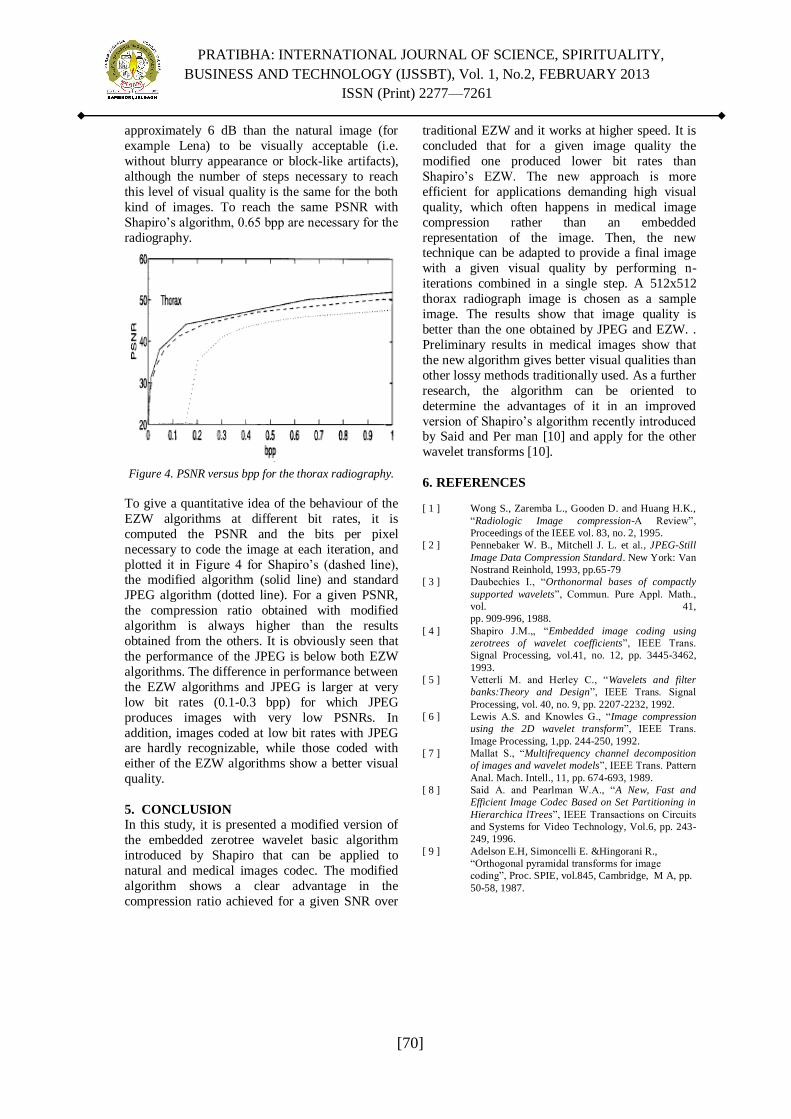
PRATIBHA: INTERNATIONAL JOURNAL OF SCIENCE, SPIRITUALITY,
BUSINESS AND TECHNOLOGY (IJSSBT), Vol. 1, No.2, FEBRUARY 2013
ISSN (Print) 2277—7261
[70]
approximately 6 dB than the natural image (for
example Lena) to be visually acceptable (i.e.
without blurry appearance or block-like artifacts),
although the number of steps necessary to reach
this level of visual quality is the same for the both
kind of images. To reach the same PSNR with
Shapiro‘s algorithm, 0.65 bpp are necessary for the
radiography.
Figure 4. PSNR versus bpp for the thorax radiography.
To give a quantitative idea of the behaviour of the
EZW algorithms at different bit rates, it is
computed the PSNR and the bits per pixel
necessary to code the image at each iteration, and
plotted it in Figure 4 for Shapiro‘s (dashed line), the modified algorithm (solid line) and standard
JPEG algorithm (dotted line). For a given PSNR,
the compression ratio obtained with modified
algorithm is always higher than the results
obtained from the others. It is obviously seen that
the performance of the JPEG is below both EZW
algorithms. The difference in performance between
the EZW algorithms and JPEG is larger at very
low bit rates (0.1-0.3 bpp) for which JPEG
produces images with very low PSNRs. In
addition, images coded at low bit rates with JPEG are hardly recognizable, while those coded with
either of the EZW algorithms show a better visual
quality.
5. CONCLUSION
In this study, it is presented a modified version of
the embedded zerotree wavelet basic algorithm
introduced by Shapiro that can be applied to
natural and medical images codec. The modified
algorithm shows a clear advantage in the
compression ratio achieved for a given SNR over
traditional EZW and it works at higher speed. It is
concluded that for a given image quality the
modified one produced lower bit rates than
Shapiro‘s EZW. The new approach is more
efficient for applications demanding high visual
quality, which often happens in medical image
compression rather than an embedded
representation of the image. Then, the new technique can be adapted to provide a final image
with a given visual quality by performing n-
iterations combined in a single step. A 512x512
thorax radiograph image is chosen as a sample
image. The results show that image quality is
better than the one obtained by JPEG and EZW. .
Preliminary results in medical images show that
the new algorithm gives better visual qualities than
other lossy methods traditionally used. As a further
research, the algorithm can be oriented to
determine the advantages of it in an improved
version of Shapiro‘s algorithm recently introduced by Said and Per man [10] and apply for the other
wavelet transforms [10].
6. REFERENCES
[ 1 ] Wong S., Zaremba L., Gooden D. and Huang H.K.,
―Radiologic Image compression-A Review‖,
Proceedings of the IEEE vol. 83, no. 2, 1995.
[ 2 ] Pennebaker W. B., Mitchell J. L. et al., JPEG-Still
Image Data Compression Standard. New York: Van
Nostrand Reinhold, 1993, pp.65-79
[ 3 ] Daubechies I., ―Orthonormal bases of compactly
supported wavelets‖, Commun. Pure Appl. Math.,
vol. 41,
pp. 909-996, 1988.
[ 4 ] Shapiro J.M.,, ―Embedded image coding using
zerotrees of wavelet coefficients‖, IEEE Trans.
Signal Processing, vol.41, no. 12, pp. 3445-3462,
1993.
[ 5 ] Vetterli M. and Herley C., ―Wavelets and filter
banks:Theory and Design‖, IEEE Trans. Signal
Processing, vol. 40, no. 9, pp. 2207-2232, 1992.
[ 6 ] Lewis A.S. and Knowles G., ―Image compression
using the 2D wavelet transform‖, IEEE Trans.
Image Processing, 1,pp. 244-250, 1992.
[ 7 ] Mallat S., ―Multifrequency channel decomposition
of images and wavelet models‖, IEEE Trans. Pattern
Anal. Mach. Intell., 11, pp. 674-693, 1989.
[ 8 ] Said A. and Pearlman W.A., ―A New, Fast and
Efficient Image Codec Based on Set Partitioning in
Hierarchica lTrees‖, IEEE Transactions on Circuits
and Systems for Video Technology, Vol.6, pp. 243-
249, 1996.
[ 9 ] Adelson E.H, Simoncelli E. &Hingorani R.,
―Orthogonal pyramidal transforms for image
coding‖, Proc. SPIE, vol.845, Cambridge, M A, pp.
50-58, 1987.

PRATIBHA: INTERNATIONAL JOURNAL OF SCIENCE, SPIRITUALITY,
BUSINESS AND TECHNOLOGY (IJSSBT), Vol. 1, No.2, FEBRUARY 2013
ISSN (Print) 2277—7261
[71]
Classification of Faults on 400 KV Transmission Line
Dr.M.A.BEG1 N.G.BUNDHE
2 S.R.PARASKAR
3
1,Shri Sant Gajanan Maharaj College of engineering Shegaon 2Mauli college Of engineering and technology,Shegaon
Abstract: The Prime aim of Power System is to
provide uninterrupted Power supply to
consumers but the performance of Power
system is frequently affected by transmission
line faults. This fault may occur due to stormy
weather, lightening strokes and overhead
transmission line failure due to ageing of
equipments etc which finally lead to disruption
in power flow. In order to maintain the
continuity of supply and to improve the
efficiency of Power System the transmission line
fault should be diagnosed and treated
accurately. This paper describes the
development of Wavelet-ANN method for
classification of Faults on a HV network.
The disturbances characterized are
events from an actual, simplified 400KV
transmission system of Maharashtra State
Electricity transmission company limited
(MSETCL) with actual line parameters. The
main purpose of the algorithm is to classify the
fault, where the fault types that can be classified
are single-line-to-earth fault (LG), double line
fault (LL), double line to earth fault (LLG) and
three phase fault (LLL).
Keywords: Discrete Wavelet Transform, Artificial
Neural Network, Transmission Line Faults
I .Introduction Among the power system components the
transmission lines are mostly affected since they
are exposed to environment. In order to ensure the
quality performance of power system the proper
classification of fault is essential. Different
techniques have been proposed to classify the
faults. Dash PK et al. [1] simulated the real power
system model using PS block set of simulink
(Matlab). Faults are conducted at different
location, fault resistance and inception angle. The
HS transform based time frequency analysis of
current signals was performed and on the visual basis faults are classified. Classification of fault on
visual basis is not reliable process. M. Jayabharata
Reddy and D.K. Mohanta [2] presented DSP based
frequency domain approach for classification of
transmission line faults using a sample three phase
power system simulated in MATLAB software.
The line currents were processed using online
wavelet transform algorithm to obtain wavelet
MRA coefficient. The algorithm has used sixth
level detailed coefficient values of current for
classification purpose. The suggested algorithm in
this paper involves too much mathematical
computation. P. S. Bhowmik et al. [3] used a
portion of west Bengal state Electricity Board
Power transmission system with actual line
parameters as a source of study. The fault conditions were simulated using EMTP. DWT
was used as a tool to process the fault voltage
signal. Some meaningful features were extracted
from the processed signal and fed to ANN for
classification purpose. K.M.Silva et al. [4]
proposed a novel method for fault detection and
classification in transmission lines with the help of
oscillographic record analysis. In module (1) i.e.
detection of fault, the fault current and voltage
sample were normalized and processed using
DWT. In 2nd module once the fault is detected the
samples related to fault clearing time were chosen and resampling of waveform was performed.
Further with the help of windowing process, each
window was analyzed through the ANN to classify
the fault. Dalstein et al. [5] simulated the faults on
a 380KV Transmission line with the help of
simulation Program Netomac. Five consecutive
sample points of normalized voltage and current of
each line according to fault type are used as input
to ANN. Therefore the 30 input nodes were build
and ANN has to provide the 11 output nodes. One
of these 11 output mapped to a value 0.9 and all the other valued mapped to 0.1. Hence this net is
trained to learn that winner takes all problems.
G. Sudha and T. Basavaraju [6] suggested the
study of three approaches that effectively classify
all types of transmission line faults. The study is
performed in MATLAB, since it provides
interactive environment among toolboxes like
wavelet transform, fuzzy interference system and
simulink, making programming and transfer of
data between program modules simpler.
This paper describes the development of
Wavelet-ANN method for classification of Faults on a HV network. The disturbances characterized
are events from an actual, simplified 400KV
transmission system of Maharashtra State
Electricity transmission company limited
(MSETCL) with actual line parameters. The fault
conditions are simulated in PSCAD software on
the AKOLA-KORADI 250 km long transmission
line .Fault signals in each case are extracted to
several scales on the wavelet transforms, and then

PRATIBHA: INTERNATIONAL JOURNAL OF SCIENCE, SPIRITUALITY,
BUSINESS AND TECHNOLOGY (IJSSBT), Vol. 1, No.2, FEBRUARY 2013
ISSN (Print) 2277—7261
[72]
certain selected features of the wavelet
transformed signals are used as an input for a
training the neural networks. The features which
are provided as an input to ANN includes
maximum and minimum level 3 and level 4
detailed coefficients of line voltage and energies of
level 3 and level 4 detailed coefficients of current.
The main purpose of the algorithm is to classify the fault.
II. WAVELET TRANSFORM
The transform of a signal is just another form of
representing the signal. The Wavelet Transform
provides a time-frequency representation of the
signal and uses multi-resolution technique by which different frequencies are analyzed with
different resolutions. The wavelet analysis
described is known as the continuous wavelet
transform or CWT. More formally it is written as:
-----1
Where * denotes complex conjugation.
This equation 1 shows how a function f(t) is
decomposed into a set of basis functions called the
wavelets. The variables s and �, scale and
translation parameters respectively are the new
dimensions after the wavelet transform.The Wavelet Series is just a sampled version of CWT
and its computation may consume significant
amount of time and resources, depending on the
resolution required. The Discrete Wavelet
Transform (DWT), which is based on sub-band
coding, is found to yield a fast computation of
Wavelet Transform. It is easy to implement and
reduces the computation time and resources
required.
Ψ (t-k / ) ------- 2
In equation (2) j and k are integers and s0 > 1 is a
fixed dilation step. The translation factor odepends on the dilation step. In the case of DWT,
a time-scale representation of the digital signal is
obtained using digital filtering techniques. The
signal to be analyzed is passed through filters with
different cut off frequencies at different scales. The
DWT is computed by successive lowpass and
highpass filtering of the discrete time-domain
signal . . The figure (1) shows the signal with sampling frequency of 200Khz denoted by the
sequence x[n], where n is an integer. This signal is
decomposed upto level 4 and frequency bands
contained in each level are represented in figure.
The low pass filter is denoted by G0 while the high
pass filter is denoted by H0. At each level, the high
pass filter produces detail information d[n], while
the low pass filter associated with scaling function
produces coarse approximations, a[n].
Fig 1.Wavelet decomposition tree
III. NEURAL NETWORKS
ANN is defined as a computing system
made up of a number of simple, highly interconnected processing elements, which process
information by their dynamic state response to
external inputs.
Neural networks are typically organized
in layers made of a number of interconnected
‗nodes‘ which contain ‗activation function‘.
Patterns are presented to the network via the ‗input
layer‘, which communicates to one or more
‗hidden layers‘ where the actual processing is done
via a system of weighted ‗connection‘. The hidden
layers then link to an ‗output layer‘ as shown in the Fig 2
Fig.2 ANN architecture
An input is presented to the neural network
and a corresponding desired target response is set
at the output. An error is composed from the difference between the desired response and the
system output. This error information is fed back
to the system and adjusts the system parameters in
a systematic fashion (the learning rule). The
process is repeated until the performance is
acceptable.The performance of ANN hinges
heavily on the data. If one does not have data that

PRATIBHA: INTERNATIONAL JOURNAL OF SCIENCE, SPIRITUALITY,
BUSINESS AND TECHNOLOGY (IJSSBT), Vol. 1, No.2, FEBRUARY 2013
ISSN (Print) 2277—7261
[73]
cover a significant portion of the operating
conditions or the data is noisy, then neural network
technology is probably not the right solution. On
the other hand, if there is plenty of data and the
problem is poorly understood to derive an
approximate model, then neural network
technology is a good choice.
IV. SIMULATED SYSTEM
MSETCL 400KV network shown in Fig (3)
consists of total 28 buses out of which 20 are the
intrastate buses and 8 are the interstate buses. This
network also includes 55Transmission Lines, Four
generating buses and 16 LOAD buses. Additional
power require to fulfill the demand is imported from inter-state generator namely Bhilai,
Khandwa, Sardarsarovar, Boisar, Bhadravati,
Tarapur, Satpura, and Mapusa.
Fig 3: MSETCL 400KV network
In this Paper 400KV MSETCL network is
simulated in PSCAD software with a sampling
frequency of 200 KHZ. Different types of fault
LG, LL, LLG and LLL are created at different
locations on the AKOLA-KORADI 250 km long
transmission line at an interval of 20 km including
the different inception angle 0, 45, and 90 degrees.
So in all 13 fault locations, three inception fault
angles and four different types of faults
(13*3*4=156) constitute 156 cases. The data from
the single end from AKOLA bus is used for the
classification of faults.
V. Feature extraction:
The line voltages and phase current signals of simulated system are recorded for a time period of
2cycles.i.e.1 prefault cycle and 1 during fault
cycle. To extract some selected feature these line
voltages and phase current signals are decomposed
up to fourth detail level using Daubechies-3 (db3)
as a mother wavelet. DWT is used since it is one
of the best tools to analyses non stationary signal.
Daubechies-3 (db3) wavelet is employed since it
has been demonstrated to perform well.
The features extracted by processing the wavelet
coefficient are maximum and minimum d3 and d4
level detailed coefficients of line voltages and energies of d3 and level d4 level detailed
coefficients of phase currents . This analysis is
performed on the Akola bus. The features
obtained by processing the wavelet coefficient are
provided as an input to ANN for the classification
purpose. The analysis in case of LG fault is shown
in fig.5,6,7
Fig 4.The proposed methodology of fault classification

PRATIBHA: INTERNATIONAL JOURNAL OF SCIENCE, SPIRITUALITY,
BUSINESS AND TECHNOLOGY (IJSSBT), Vol. 1, No.2, FEBRUARY 2013
ISSN (Print) 2277—7261
[74]
Fig5.Wavelet decomposition of line voltage signal in
case of LG fault
Fig6. Maximum and minimum d3 and d4level dwt
coefficient in case of LG fault
Fig7.Energy of d3 and d4 level dwt coefficient in case of LG fault
VI. Result and Discussion
The Frequency-Dependent Line Model is
selected for simulation of 400 KV system because
it is the most accurate and it represents all
frequency dependent effects of a transmission line.
The faults cannot be distinguished merely by
observing the simulated system waveform hence
processing of signal is necessary. The phase
current and line voltage signals are processed for
prefault and during fault cycle using dwt. However
the discrimination of fault is not possible just with the help of dwt transformed signals. Finally some
distinguishing features were derived from the dwt
transformed signal. The features include the
maximum and minimum d3 and d4 level dwt
coefficient of line voltages along with the energy
of d3 and d4 level dwt coefficient of phase
currents. The energy of signal is given as
where x(i) is the discrete sequence
representing maximium and minimum d3 and d4level dwt coefficient of phase currents.These
distinguishing features are provided as an input to
ANN.
Some previous studies offer guidelines for
selecting the architecture of ANN. Various
training methods were used for ANN. In this paper
Multilayer perceptron (MLP) neural network is
used with combination of momentum leaning rule
and tanhaxon axon is chosen as node activation
function. The choice of 1 hidden layer with 10
processing element (PE) provides the 100% correct fault classification.
D3Max
D3Min
D4Max
D4Max
Vab 30.5 -117 258. -77.
Vbc 117. -30. 77.0 -259
Vca 0.99 -0.9 1.58 -1.6
-300
-200
-100
0
100
200
300M
A
G
N
I
T
U
D
E
Max and Min level 3 and level 4 detailed dwt coefficient
LG
Ea Eb Ec
L3 0.03318226 0.10974438 0.03316280
L4 0.14838778 3.13867338 0.14834435
0
0.5
1
1.5
2
2.5
3
3.5M
A
G
N
I
T
U
D
E
Energy of current dwt detailed coefficient
LG

PRATIBHA: INTERNATIONAL JOURNAL OF SCIENCE, SPIRITUALITY,
BUSINESS AND TECHNOLOGY (IJSSBT), Vol. 1, No.2, FEBRUARY 2013
ISSN (Print) 2277—7261
[75]
Fig8. No. Of processing element Vs classification
accuracy
VII. Conclusion
A new generalised algorithm to classify the faults
occuring on High Voltage transmission line is
developed in the paper. In the present work a
400KV MSETCL system is simulated in PSCAD
with actual line parameters. DWT with its inherent
time frequency localization property is employed
to extract discriminating features from the phase
currents and line voltages. A back propagation
neural network classifier is then used for
identification of fault type. Faults with various
types, conditions and location have been tested and hundred percent accurate classifications are
obtained.
The results obtained with the use of
DWT-ANN based algorithm are promising and
suggest that this approach could lead to useful
application in an actual power system.
REFERENCES [1] Dash PK and Samantaray SR ― A novel distance
protection scheme using time–frequency analysis and
pattern recognition approach‖. Int J Elect Power Energy
system 2006
[2] M. Jayabharata Reddy and D.K. Mohanta ― A DSP
based frequency domain approach for classification of
transmission line faults ―Science Direct Digital Signal
Processing 18 (2008) pp. 751–761
[3] P. S. Bhowmik, P. Purkait Member and K. Bhattacharya
― A Novel Wavelet Assisted Neural Network for
Transmission Line Fault Analysis‖ Electrical Power and
Energy Systems 31 (2009) pp.213–219
[4] K.M.Silva B.A.Souza andN.S.D.Brito ―Fault Detection
and Classification in Transmission Lines Based on
Wavelet Transform & ANN‖ IEEE TRANSACTIONS
ON POWER DELIVERY, VOL. 21, NO. 4, OCTOBER
2006 pp.2058-2063
[5] Dalstein and B. Kulicke, ―Neural network approach to
fault classification for high speed protective relaying‖,
IEEE Trans. Power Del., vol.10, pp. 1002-1009, 1995.
[6] G. Sudha , T. Basavaraju B.I.T, V.T.U, Bangalore, India
‖A comparison between different approaches for fault
classification in transmission line‖ IET-UK International
Conference on Information and Communication
Technology in Electrical Sciences (ICTES 2007) Dr.
M.G.R. University, Chennai, Tamil Nadu, India. Dec. 20-
22- 2007. pp.398-403.

PRATIBHA: INTERNATIONAL JOURNAL OF SCIENCE, SPIRITUALITY,
BUSINESS AND TECHNOLOGY (IJSSBT), Vol. 1, No.2, FEBRUARY 2013
ISSN (Print) 2277—7261
[76]
Investigation of Human Resource Management Practices
(HRM) in Hospitals of Jalgaon District
Saroj B. Patil*; Dr. P.T.Choudhari** *Research Scholar, North Maharastra University, Jalgaon, India.
** Head, Department of Commerce, M.J. College, Jalgaon, India
Email:*[email protected]
ABSTRACT
This study is aimed to investigate, identify and
compare Human Resource Management
(HRM) practices in government and private
hospitals of Jalgaon District. Self developed
questionnaire; based on literature reviews are
an instrument used for data collection.The
findings of this study are important for
understanding the needs of human resource
management practices in hospitals,
contributions of different factors towards
quality care of patients and work culture among
the staff.
Keywords: HRM, Hospital
INTRODUCTION
Human behavior means, how the people react to
situation, what motivate the people and how
organization create an environment for people to
feel comfort and work independently. Human
resource management not only deals with
individuals but with team work. Work together to
give best output management task is for ensuring a
success and motivated workforce and deal with work place environment.
Human resource management in health sector
seeks to improve the quality of services and
patients satisfaction. Health care quality is
generally defined in two ways: technical quality
and socio-cultural quality. Technical refers to the
impact that the health services available can have
on the health condition population. Socio-cultural
quality measures the degree of acceptability of
services and the ability to satisfy patient
expectations. Better use of the spectrum of health
care providers and better co-ordination of patient services through inter disciplinary team work have
been required as a part of human resource
management. Since all health care is ultimately
delivered by people, effective human resource
management will play a vital role in the success of
health policies in any nation.
Fisher (1991) and Spreitzer (1998) suggest that
trust in management and perceptions that
downsizing was handled in a justifiable manner
can lead to reduced threat and greater cooperation
from staff. Spector (1997) said that ―job
satisfaction is the most frequently studied variable
in organizational behavior reach‖. He discussed the reason why we should be concerned with job
satisfaction. He concluded that, ―job satisfaction is
to some extent a reflection of good treatment‖ and
―it can lead to behavior by employees that affect
organizational functioning‖.
Objectives of the study are -
1. To identify the HRM practices in
hospitals
2. To compare HRM policy and practices in
government and private hospitals.
3. To propose workable suggestions to improve HRM in hospitals.
METHODOLOGY
HRM practices were analyzed to identify the
influence of these practices on job satisfaction
level of nurses through defined questionnaire for
doctors i.e. hospital administrators. By using the
Chi-square value, p-value, count value, cross
tabulations and sample percentage value
interpretations were developed. All statistical data
is also represented by suitable charts in presentable manners for better understanding. Further, all the
variables were tested by using Chi-Square test to
test the hypothesis that made an adequate and
satisfactory determination.
ANALYSIS AND FINDINGS
The researcher used a questionnaire for collecting
the data. The data is analyzed and results are
graphically presented as below:
A. Human Resource planning development
i. Vision and mission displayed
In government hospitals the mission and vision are
promulgated by the ministry of health and welfare.
They are mandatorily displayed. The nurses are more aware about them and there is an equality of
private hospitals also to do so for their professional
reasons. The result is that 66.67% of the doctors in
government hospitals and 63.0% of the private
hospital doctors agreed that vision and mission of
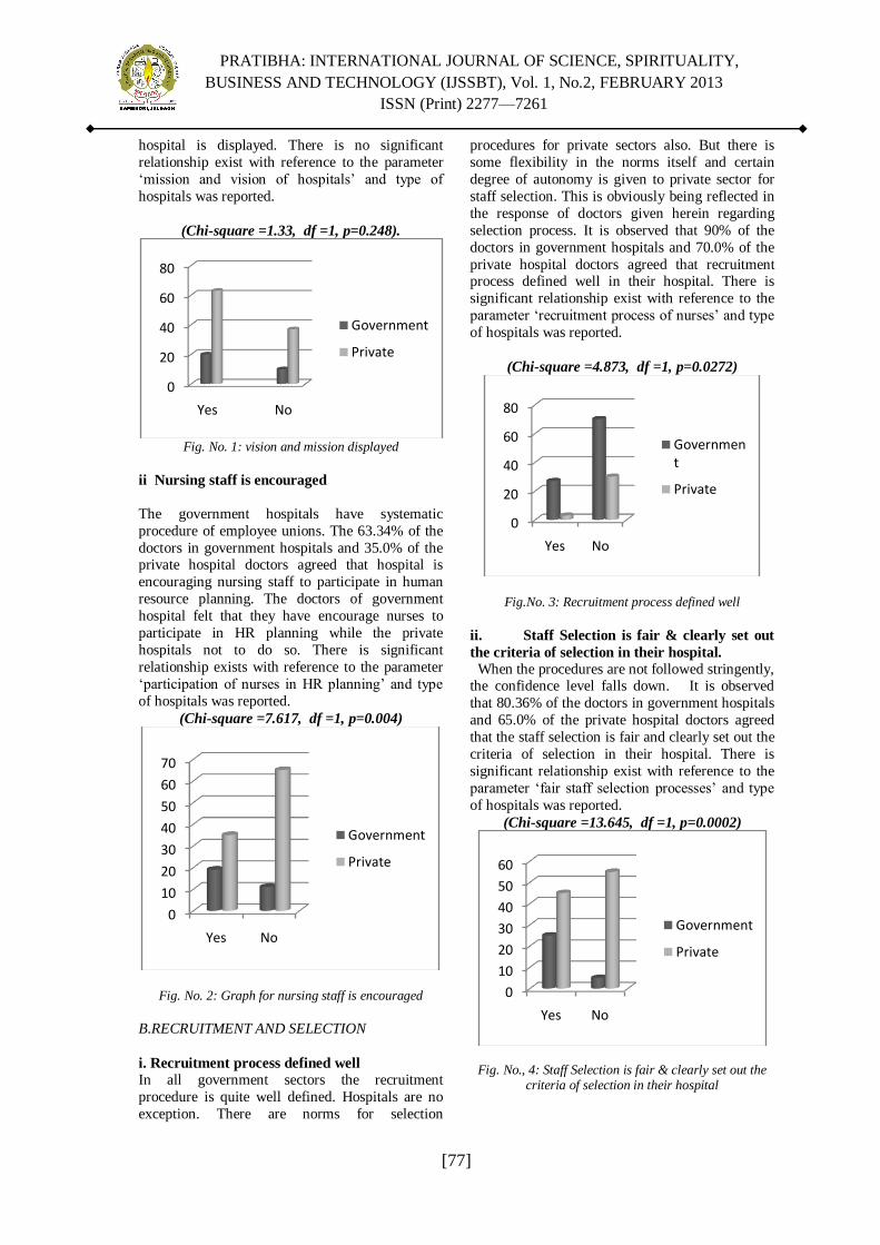
PRATIBHA: INTERNATIONAL JOURNAL OF SCIENCE, SPIRITUALITY,
BUSINESS AND TECHNOLOGY (IJSSBT), Vol. 1, No.2, FEBRUARY 2013
ISSN (Print) 2277—7261
[77]
hospital is displayed. There is no significant
relationship exist with reference to the parameter
‗mission and vision of hospitals‘ and type of
hospitals was reported.
(Chi-square =1.33, df =1, p=0.248).
Fig. No. 1: vision and mission displayed
ii Nursing staff is encouraged
The government hospitals have systematic
procedure of employee unions. The 63.34% of the
doctors in government hospitals and 35.0% of the private hospital doctors agreed that hospital is
encouraging nursing staff to participate in human
resource planning. The doctors of government
hospital felt that they have encourage nurses to
participate in HR planning while the private
hospitals not to do so. There is significant
relationship exists with reference to the parameter
‗participation of nurses in HR planning‘ and type
of hospitals was reported.
(Chi-square =7.617, df =1, p=0.004)
Fig. No. 2: Graph for nursing staff is encouraged
B.RECRUITMENT AND SELECTION
i. Recruitment process defined well
In all government sectors the recruitment
procedure is quite well defined. Hospitals are no
exception. There are norms for selection
procedures for private sectors also. But there is
some flexibility in the norms itself and certain
degree of autonomy is given to private sector for
staff selection. This is obviously being reflected in
the response of doctors given herein regarding
selection process. It is observed that 90% of the
doctors in government hospitals and 70.0% of the
private hospital doctors agreed that recruitment process defined well in their hospital. There is
significant relationship exist with reference to the
parameter ‗recruitment process of nurses‘ and type
of hospitals was reported.
(Chi-square =4.873, df =1, p=0.0272)
Fig.No. 3: Recruitment process defined well
ii. Staff Selection is fair & clearly set out
the criteria of selection in their hospital.
When the procedures are not followed stringently, the confidence level falls down. It is observed
that 80.36% of the doctors in government hospitals
and 65.0% of the private hospital doctors agreed
that the staff selection is fair and clearly set out the
criteria of selection in their hospital. There is
significant relationship exist with reference to the
parameter ‗fair staff selection processes‘ and type
of hospitals was reported.
(Chi-square =13.645, df =1, p=0.0002)
Fig. No., 4: Staff Selection is fair & clearly set out the criteria of selection in their hospital
0
20
40
60
80
Yes No
Government
Private
0
10
20
30
40
50
60
70
Yes No
Government
Private
0
20
40
60
80
Yes No
Government
Private
0
10
20
30
40
50
60
Yes No
Government
Private

PRATIBHA: INTERNATIONAL JOURNAL OF SCIENCE, SPIRITUALITY,
BUSINESS AND TECHNOLOGY (IJSSBT), Vol. 1, No.2, FEBRUARY 2013
ISSN (Print) 2277—7261
[78]
C. PERSONAL POLICIES
i. Career development scheme exists in their
hospital.
The ministry of health and welfare of
central and state governments have initiated
several schemes for the welfare of nursing staff. Government hospitals are at top position for
implementing the development scheme and their
nursing staff is getting benefit of these schemes.
But private hospitals are lagging behind to take the
benefit of such schemes. It is observed that 63.36%
of the doctors in government hospitals and 38.0%
of the private hospital doctors agreed that career
development scheme exists in their hospital. There
is significant relationship exist with reference to
the parameter ‗career development scheme exists‘
and type of hospitals was reported.
(Chi-square =6.015, df =1, p=0.0141)
Fig. No.5: Career development scheme exists in their hospital
ii. Hospital handles staff needs and demands
properly.
It is a very positive observation that both the
category of doctors has reported that the needs of
staff are handled properly. This proportion is even
higher in the private hospitals. This may be
because the fact that they have a personal attention
to the staff and they are concerned with the output quality. It is observed that 86.66% of the doctors
in government hospitals and 98% of the private
hospital doctors agree that hospital handles staff
needs and demands properly. There is significant
relationship exist with reference to the parameter
‗staff needs and demands‘ and type of hospitals
were reported.
(Chi-square =6.733, df =1, p=0.009).
Fig. No. 6: Hospital handles staff needs and demands
properly
D.PRACTICES FOR EMPLOYEE BENEFITS
i. Group/individual insurance policy is exist in their hospital.
Insurance policies are the most helping hands to
the employees those are working in government
hospitals and private hospital. These insurance
policies minimize the future risk and financial
needs when big sort of problem arises.
Government hospitals are always following their
norms for group insurance policy or individual
insurance policy. Government hospitals have clear-
cut mechanism for insurance of nursing staff. In
this regard there are government directives for private hospitals also. But the insurance policies
are not well implemented in the private hospitals.
Such practices need to be practiced in private
hospitals too. It has been found that 66.66% of the
doctors in government hospitals and 15% of the
private hospital doctors agreed that
group/individual insurance policy is exist in their
hospital. There is significant relationship exist
with reference to the parameter ‗an insurance
policy of nurses‘ and type of hospitals was
reported.
(Chi-square =31.311, df =1, p=2.19831E-08)
Fig No. : 7: Group/individual insurance policy is exist in
their hospital.
0
20
40
60
80
Yes No
Government
Private
0
20
40
60
80
100
Yes No
Government
private
0
50
100
Yes No
Government
Private

PRATIBHA: INTERNATIONAL JOURNAL OF SCIENCE, SPIRITUALITY,
BUSINESS AND TECHNOLOGY (IJSSBT), Vol. 1, No.2, FEBRUARY 2013
ISSN (Print) 2277—7261
[79]
ii. Reimbursing for skill development activities.
Hospital management arranges variety of the
training programme and workshops for skill
development. It has been observed that 70.0% of
the doctors in government hospitals and 55.0% of
the private hospital doctors are agreed that their
hospitals are reimbursing for skill development activities. There is no significant relationship exist
with reference to the parameter ‗Nurses
reimbursed for skill development activities‘ and
type of hospitals was reported.
(Chi-square =2.138, df =1, p=0.143)
Fig. No. 8: Reimbursing for skill development activities.
E. WORKPLACE MANAGEMENT
i. Clerical duties are performed by clerical staff
in their hospital
It is clear that the private hospital nurses are being
overloaded. In addition to their regular work, they
are additionally being loaded with the clerical
work. This situation must be changed. Private
hospitals must involve adequate number of clerical
staff for such duties. It is observed that 96.67% of
the doctors in government hospitals and 65.0% of
the private hospital doctors agreed that clerical
duties are performed by clerical staff in their
hospital. There is significant relationship exists
with reference to the parameter ‗job responsibility
other than nursing staff‘ and type of hospitals was reported.
(Chi-square =11.557, df =1, p=0.0006)
Fig. No. 9: Clerical duties are performed by clerical
staff in their hospital
ii. Hygiene and safety are emphasized in their
hospital.
It is very pleasant to see that doctors from both
the sectors felt that hygiene and safety is being
practiced properly in the hospitals. It is observed
that 96.67% of the doctors in government hospitals
and 85.0% of the private hospital doctors agreed that hygiene and safety are emphasized in their
hospital. There is no significant relationship exist
with reference to the parameter ‗Hygiene and
safety at work places‘ and type of hospitals was
reported.
(Chi-square =2.910, df =1, p=0.0880)
Fig. No. 10: Hygiene and safety are emphasized in their
hospital.
F. EMPLOYEE RELATION AND
COMMUNICATION
i. Hospital promote corporative
interdisciplinary relationships
It is quite positive to see that in government
hospitals there is a flexibility to promote
corporative interdisciplinary relations. In private
hospitals this proportion is very low. This is a
matter of concern. Hospitals authorities must
seriously investigate the causes for this and must
do required changes to promote corporative
interdisciplinary relationship. It is observed that
96.66% of the doctors in government hospitals and
30% of the private hospital doctors agreed that their hospital promote corporative interdisciplinary
relationships. There is significant relationship exist
with reference to the parameter ‗promotion of co-
operative inter disciplinary relationship‘ and type
of hospitals was reported.
(Chi-square =41.378, df =1, p=1.25461E-10)
0
20
40
60
Yes No
Government
Private
0
20
40
60
80
Yes No
Government
Private
0
20
40
60
80
100
Yes No
Government
Private

PRATIBHA: INTERNATIONAL JOURNAL OF SCIENCE, SPIRITUALITY,
BUSINESS AND TECHNOLOGY (IJSSBT), Vol. 1, No.2, FEBRUARY 2013
ISSN (Print) 2277—7261
[80]
Fig. No. 11: Hospital promote corporative
interdisciplinary relationships
ii. Nurses participated in hospital management
practices.
In the present era of liberalization and
globalization, employees have instinct urge to
participate in management up to certain limit. The
observation is that 16.67% of the doctors in
government hospitals and 1% of the private
hospital doctors agreed that nurses participated in
hospital management practices. There is significant
relationship exists with reference to the parameter
‗Nurses participate in hospital management‘ and type of hospitals was reported.
(Chi-square =12.866, df =1, p=0.0003)
Fig. No. 12: Nurses participated in hospital
management practices.
G. TRAINING AND DEVELOPMENT
i. Opportunities for continuing education are
available in their hospital.
Education is the process to achieve excellence and develop the creative and innovative sights in human being. It is therefore necessary to give opportunity for continuing education. It is a positive sign to see that both private hospital and government hospital doctors reported that they are given opportunities for continuing education. It is observed that 100.0% of the doctors in government hospital and 95.0% of the private doctors agreed
that opportunities for continuing education are
available in their hospital. There is no significant
relationship exist with reference to the parameter
‗Opportunities for continuing education are
available‘ and type of hospitals was reported.
(Chi-square =3.250, df =1, p=0.071423)
Fig. No. 13: Opportunities for continuing education are
available in their hospital
H. EMPLOYEE WELFARE AND
COMPENSATION
i. Excellence in human resource management
practices.
It is observe that 96.67% of the doctors in
government hospital and 0% of the private doctors
agreed that fringe benefits (PF, Gratuity, Uniform,
Recreation. etc) are given in their hospital. It is
serious concern for private hospitals administrators
to achieve the excellence in human resource
management practices. There is significant
relationship exist with reference to the parameter
‗fringe benefits‘ and type of hospitals was
reported.
(Chi-square =124.422, df =1, p=6.81043E-29)
Fig. No. : 14: Excellence in human resource
management practices
ii. Post retirement benefit program
It is observed that 100.0% of the doctors in
government hospitals and none of the private
hospital doctor agreed that the post retirement
benefit program is existing in their hospital. It must
be improved in private hospitals. There is
significant relationship exist with reference to the
parameter ‗post retirement benefits‘ and type of
hospitals was reported.
Gover…0
50
100
Yes
Government
Private
0
20
40
60
80
100
Yes No
Government
Private
0
20
40
60
80
100
Yes No
Government
Private
0
50
100
Yes No
Government
Private

PRATIBHA: INTERNATIONAL JOURNAL OF SCIENCE, SPIRITUALITY,
BUSINESS AND TECHNOLOGY (IJSSBT), Vol. 1, No.2, FEBRUARY 2013
ISSN (Print) 2277—7261
[81]
(Chi-square =185, df =1, p=392462E-42)
Fig. No 15 . : Post retirement benefit program
CONCLUSION
The present study leads to the conclusion that
HRM practices are very skill fully applied by
private hospitals. They have applied all superficial practices in higher proportion as compared to the
government hospitals. However the core practices
are applied only in Government hospitals. In fact
these practices are dictated by the service norms of
government employees and are reflected in other
professions too.
It is very interesting to note that the private
hospitals are more skilled in customer oriented
training of their staff. In government hospitals,
there is a routine practice of senior officials taking
meeting of staff and taking feedback and report from staff regarding target compliances. In fact
targets are the specific tasks given to staff in
government hospital that is in conjunction with the
mission and vision. In private hospitals, nurses do
not have such ―targets‖ and field jobs are limited to
the clinical cares only. Thus about the mission and
vision there awareness is less. These are a positive
indication that more than 80% of staff in private
hospitals well as government hospitals have
accepted that their organizational goals are for
good causes. An unsatisfied employee would have
less faith in the genuineness of organizational
goals. It is very positive sign that the working
procedures are well known to the very large
proportion of employees. Further the percentage is
higher for government hospitals. These are because
government hospitals have many well established
procedures as compared to the private hospitals. The administrative approaches of the government
hospitals as compared to the private hospitals are
more flexible. It is hoped that the present study
will form a suitable data base for hospitals to
retrospect their HRM practices and to enhance
them for better HRM outcome.
REFERENCES
[1] Kavya Sharma, Sanjay Zope, ―Health and Hospital
Management Education in India‖. ISSN 2229-337X, Vol-
2, Issue 1. Jan – 2011.
[2] Nahid Dehghan Nayeri Ali Akbar Nazari, ―Iranian staff
nurses view of their productivity and human resources
factor improving and impeding it::a quality study‖.
[3] Linda Mcgillis hall, ― Nursing intellectual capital: a
theoretical approach for analyzing nursing productivity‖,
Jan-2003
[4] Thomay A-Slay, Thesis entitled as , ―Intrinsic and
extrinsic factor affecting job satisfaction of nursing
assistants in two long term care.‖
[5] Aswathappa K., ― Human Resource Management- Text &
Cases‖, Tata McGraw Hill, 6th edition,2010
[6] Menon P.K.S., ―Human Resource Management and
Organizational Behavior‖, Himalaya Publishing House,
2005
[7] Manoria C.B., Gankar S.V., ― A Textbook of Human
Resource Management‖, Himalaya Publishing House,
2010
[8] Wayne R., ―Human Resource Management‖, SPHR, 10th
edition, Pearson Publications.2010, ISBN 978 – 81 -317 -
2568 -9
[9] Mutsuddi Indranil, ― Essentials of Human Resource
Management‖, New Age international Publishers, 2010,
ISBN 978 – 81 – 224 -2815 -5
0
20
40
60
80
100
Yes No
Government
Private

PRATIBHA: INTERNATIONAL JOURNAL OF SCIENCE, SPIRITUALITY,
BUSINESS AND TECHNOLOGY (IJSSBT), Vol. 1, No.2, FEBRUARY 2013
ISSN (Print) 2277—7261
[82]
Role of Constitutional Ruling System
Sakina Husain1, Dr M Husain
2 and Dr K S Wani
3
1. Formerly Lecturer, Dr Jakir Husain Academy, College of Science, Arts and Commerce,
Burhanpur, MP.
2. Professor, Civil Engineering, SSBT‘s College of Engineering and Technology, Bambhori,
Jalgaon, MS.
3. Principal, SSBT‘s College of Engineering and Technology, Bambhori, Jalgaon, MS.
Abstract: Indian philosophy believes that since
the ancient times, the universe was auto-
regulated. It was absolutely self-governed
without existence of formal external
governance. It was later the conscious beings
started violating the universal laws and the
inception of an external governing system
became inevitable. In the modern era, every
nation has its own governing system. In the
present era one cannot imagine a nation without
a governing system. Apart from a central
governing system at top there exists are a
multilayered governing system. Indian
philosophy considers the beginning of
governing system since the time of Ramayan.
Crowing of Lord Ram symbolizes the beginning
of good governance that protects the rights of
weaker and ensures non-violation of inherent
laws of universe. It laid certain morals and
values for ideal governance.
Is the constitution of modern Indian founded on
those ideals? What is the role of constitutional
governing system in modern society? This
paper discusses these issues with a retrospective
perspective into ancient Indian mythology and
spirituality. It does a vis-à-vis comparison of the
role model of governance presented by ancient
Indian epic Ramayan and modern India’s
constitution.
Key words: Constitution, Mythology, Spirituality,
Ramayan (The ancient Indian epic).
Introduction:
GOD is the ultimate ruler of universe. It is
a fundamental idea of human psychology and is
reflected in all spiritual and mythological thoughts
too. The word God has many synonyms in Indian
philosophy. One of the synonyms is ―Vidhi‖- the
rule or law or procedure. It is important to be seen that in the word ―vidhi‖ God is not referred as a
noun; rather as a verb. God is the creator of
―Vidhi‖, the Vidhata. Still the Indian philosophy
does not consider him to be over and above the
vidhi. The creator of universal laws (Vidhi)
himself (herself) is abided of his own universal
laws. He, the almighty as referred in most of the
spiritual philosophies is not an autocratic random
players of universal laws. It means that the creator
of laws himself is not considered to be a monarch.
This represents the supremacy of universal laws.
The universal laws owe equally highest degree of
respectability as the creator of these laws. Even the
incarnations (Avtar) also abide themselves with these universal laws (Maryada). The character of
Lord Ram is an excellent example of this and is
rightly referred as ―Marayada Purushottam‖ -the
great human who respected all the laws.
All activities in the universe are governed
by these supreme and pious laws. All materialistic
creatures strictly follow these universal laws. Yet
the conscious beings, the living creatures are given
a ―freedom of selection‖ within the universal laws.
This freedom in true sense is the wisdom of
conscious beings. The universal functioning is
going on since the infinite time according to these laws. Yet, if a conscious being attempts to violet
the universal laws, what are the inherent provisions
within the laws to prohibit such violation? What if
a mighty conscious being attempts to suppress a
weaker one? How the rights of a weaker one are
safe-guarded? The Constitutional governing
system is a provision to check such violations. In
true sense, this is the role of constitutional
governing system.
The ancient Indian mythological epic
Ramayan describes that the incarnation of Ram was for the purpose of prohibiting the violation of
pious universal laws and to establish their
supremacy. It was to basically protect the right of
weaker. Ramayan is the Constitution of Indian
philosophy. Today, the ruling system in India is
defined by the Constitution of India. The scope of
discussion of this paper is to analyze to what extent
does this constitution of modern India meets the
ideals defined by ancient Indian philosophy.
The Mythological Reference:
Once upon a time, in the farmyards (Ashram) of Sage Valmiki a couple birds were
indulged in play. Here play symbolically
represents the prevalence of an inherent peace and
satisfaction. It shows that the universal functioning
was smoothly following the course; auto-regulated
and self governed. There came a hunter. He killed
one of the birds. The other bird fell in sorrow. Sage
being in meditation saw all this. The incident

PRATIBHA: INTERNATIONAL JOURNAL OF SCIENCE, SPIRITUALITY,
BUSINESS AND TECHNOLOGY (IJSSBT), Vol. 1, No.2, FEBRUARY 2013
ISSN (Print) 2277—7261
[83]
nailed him deep in his heart. He cursed the hunter
in following words:
“Ma nishad pratishtham twang amah shaswatih
samah,
Yat Kroch mithunadikam vadhih kam mohitam.”
Meaning: O hunter you have killed the playing birds. You will never and nowhere get a peace [1;
2].
Later the sage realized that the words of
curse are in the form of a ―Shloka‖, a well versed
couplet according to the grammar of Sanskrit
language. Then the sage evolved a vision. He
wrote the great epic of Ramayan. Ramayan starts
with the words that Valmiki used to curse the
hunter. Ramayan is considered to be the first
literature created by civilization. Ramayan presents
a hypothesis of Ramrajya, the ruling of Ram. An ideal governing system. A governing system in
which the rights of weaker are not suppressed by
the stronger. The rights of weaker are protected by
the governance. It assures a kingdom which is free
from fear. According to Indian philosophy this is
the role of constitutional ruling system. In
Ramayan, the capital of Ram‘s Kingdom is
Ayadhya- a place where no yudhha (war) takes
place. Another name of Ayodhya is Avadh- a place
where no vadh (killing) takes place. These are the
ideals laid down for a governing system according to Indian mythology. This paper endeavors to
identify these ideals in the constitution of modern
India.
Ruling Patterns in Modern World:
In modern world there are varieties of
ruling patterns. They include right from pure
monarchy, military rule, communist rule, pure
democracy etc. broadly they may be categorized
into two- autocracy and democracy. The word
democracy is derived from the Latin word demo-cratine [3]. It means people to rule. Democracy is
generally considered to be a system evolved later
with civilization hence is a modern system. It is
evolved as a people beneficiary ruling system. Still
there are so many examples of so called failed
democracies and successful autocracies also. Yet
there is a fundamental difference between the two.
Autocracy in itself has no room for the opposite
thought, while democracy is based upon the
ideology of coexistence and consensus. It gives
recognition to the opposite thoughts too. It is not
just a ruling system but is a life style in broad sense. Suppression of opposite thought is violence.
Democracy is a non-violence based system.
The constitution of India:
Modern India opted democracy as a
ruling pattern. The constitution of India is the
world‘s largest written constitution which is
created refereeing all the constitutions of the
world. It has declared India to be a sovereign,
socialist and secular democratic republic [4]. It has
given right of equality to all. It is based upon the theory of no discrimination on the basis of caste,
religion, language, race, gender, color etc.. In
abstract it is based upon the theory of right is
might not might is right. It defines a ruling pattern,
a governance that safe-guards the interest of the
weakest.
An important fundamental feature of
Indian constitution is a secular governing system.
In fact Indian democracy in many ways is a role
model for the world. There are many countries
which got independence with or after India. They
preferred to opt democracy as ruling system. Yet they could not sustain long their democracy. Some
of them fell into autocracy. The Indian democracy
has sustained itself amidst all the critical situations.
This is owing to the fact that democracy is the
basis of Indian spiritual life style. In Indian
spirituality there is a room for opposite thoughts
too. Coexistence with opposite thoughts and
consensus amongst diversified thoughts are deeply
rooted in the Indian spirituality. The spiritual
philosophy of ―syadvada‖ gives allowance multiple
opinions about truth; while that of ―anekanekantvadb‖ seeks conformity and
consistency amongst diversified thoughts. Thus the
ideology of suppressing the opposite thought does
not arise; rather there is a natural ideological rise
of coexistence. Thus the democracy persists.
One more thing is important here.
Democracy and secularism go hand in hand [5]. A
ruling system based upon specific religion cannot
protect its democratic character, as it is against the
fundamental requirement of democracy that is
coexistence [6]. The world history has shown that the nations who opted religion specific ruling
system could not protect their democracy for long
time.
Conclusions:
―Ramrajya‖ is a role model of an ideal governing
system. In modern context the ideals and values of
Ramrajya is can be achieved in a well functioning
democracy. The constitution of India is truly
influenced with the ideology of Ramrajya.
Secularism is an important pillar of this system. It is very important in Indian context or in general in
the context of all eastern democracies of the globe
[7]. Once Swami Vivekananda said- ―In east one
cannot talk of politics without referring to religion,

PRATIBHA: INTERNATIONAL JOURNAL OF SCIENCE, SPIRITUALITY,
BUSINESS AND TECHNOLOGY (IJSSBT), Vol. 1, No.2, FEBRUARY 2013
ISSN (Print) 2277—7261
[84]
while in west one cannot talk of religion without
referring to the politics.‖ Consequently religion is
of supreme importance in the life style of east. Yet
our governing system is not religion specific. Our
life style is based upon consensus and coexistence.
Thus our ruling system is based upon secularism.
Hence is our democracy prevalent and persistent.
Under its umbrella the ideals of Ramrajya have scope to groom up. This finally leads to a people
beneficiary ruling system; an absolutely fearless
kingdom in which right is the might. Only a truly
civilized society can evolve such a system.
Conversely, a truly civilized system flourishes
under such a ruling system.
aSyadvad: according to Indian spirituality
―syadvad‖ is a theory which believes that no one
can be perfectly sure about reality. Or, the reality
cannot be described beyond doubt. It all depends
upon the observer‘s capacity to analyze about the reality. bAnekanekantvad: according to Indian spirituality
―anekanekantvad‖ is a theory which believes that
all different opinions about reality differ merely at
the surface; in the depth they all describe the same
reality.
References: [1] Shri Ramcharitmanas, Gita Press, Gorakhpur.
[2] Wikipedia of Ramcharitmanas.
[3] Wikipedia of political science.
[4] Pylee M V (1997) Indian Constitution, S Chand and Co.
Publication.
[5] Holyake G J (1896) The original nature of secularism,
Watts and Co. Publication, London.
[6] Wikipedia of secularism.
[7] Kosmin Barry A (2007) Contemporary Secularity and
Secularism, Publication of Institute for the study of
secularism in society and culture, Hartford.

PRATIBHA: INTERNATIONAL JOURNAL OF SCIENCE, SPIRITUALITY,
BUSINESS AND TECHNOLOGY (IJSSBT), Vol. 1, No.2, FEBRUARY 2013
ISSN (Print) 2277—7261
[85]
Response Spectrum Analysis of Asymmetrical Building
Pravin Ashok Shirule1, Bharti V. Mahajan
2
1 Associate professor, Civil Engineering Department, SSBT‘s COET, Bambhori, Jalgaon, (MS) – 425001. 2 Asst.Professor, Civil Engineering Department, Rajarshi Shahu College of Engineering, Pune.
ABSTRACT
In this project a parametric study on
Reinforced Concrete structural walls and
moment resisting frames building
representative of structural types using
response spectrum method is carried out. Here,
the design spectra recommended by Indian
Standard Code IS 1893-2002 (part I) and two
other codes (Uniform Building Code, Euro
Code 8) are considered for comparison. The
objective of this study is to investigate the
differences caused by the use of different codes
in the dynamic analysis of multistoried RC
building. To evaluate the seismic response of the
buildings, elastic analysis was performed by
using response spectrum method using the
computer program SAP2000. It is observed
from the comparative study that the base shear
using IS code is higher in all the three buildings,
when compared to that of with other codes
which leads to overestimate of overturning
moments in the building and hence heavier
structural members. To experimentally verify
the applicability of the proposed semi active
control system to torsionally coupled responses
of an asymmetric building, use of computer
software was conducted using in a G+13 storey
building model with asymmetric column
distribution.
KEYWORDS
Response spectrum analysis, Elastic design
spectra, RC building, IS code.
INTRODUCTION
Earthquake codes are periodically revised and
updated depending on the improvements in the
representation of ground motions, soils and
structures. Moreover, these revisions have been
made more frequently in recent years. The Indian Standard Code (IS 1893-2002 (Part-I)) was also
revised in 2001 and has been in effect since 2002.
This improvement was done followed to
destructive earthquake occurred in Bhuj (Gujarat
State, India) on 26th January, 2001 which resulted
in more than 19,000 recorded death and 1,66,000
injuries. Preliminary indications are that 600,000
people were left homeless, with 48,000 houses
destroyed and an additional 844,000 damaged. The
Indian State Department estimates that the
earthquake affected, directly or indirectly, 15.9
million people, nearly 50% of the population of
Gujarat. More than 20,000 cattle were reported
killed. Government estimates place direct
economic losses at $1.3 billion, although more recent estimates indicate losses may exceed $5
billion. A number of separate teams from different
bodies conducted damage surveys and reported
some conclusions as briefly summarized below.
Early reports stressed that quality of construction
were poor and that there were many structural
mistakes and deficiencies due to the non-
compliance with the earthquake code. It was
concluded that the nature of the strong-motion was
also a major contribution factor to the level of
damage. Under the light of observations and
lessons from the 2001 earthquake and past earthquakes, many studies concerning to IS 1893-
2002 have been carried out up to now and number
of improvements are made. The influence of local
ground conditions on the seismic action is
considered depending on the ground types descried
in the various codes considered in the present
study. That is why the emphasis has been given on
the differences caused by the use of spectra given
in IS Code and other well known codes such as
UBC and Euro code in the seismic analysis of
sample buildings.
Response Spectra
Response spectrum of any building gives us a plot
of peak or steady state response(Displacement,
Velocity or Acceleration) of a series of oscillators
of a varying natural frequency, that are forced into
motion by the same base vibration or shock. The
resulting plot can then be used to pick off the
response of any linear system, given its natural
frequency of oscillation. Response spectrum
analysis requires that isolator units be modeled using amplitude- dependent values of effective
stiffness. The effective damping of the isolated
modes of response is limited to 30 percent of
critical. Higher modes of response are usually
assumed to have five percent damping a value of
damping appropriate for the superstructure, which
remains essentially elastic. As previously noted,
maximum and minimum values of effective
stiffness are typically used to individually capture

PRATIBHA: INTERNATIONAL JOURNAL OF SCIENCE, SPIRITUALITY,
BUSINESS AND TECHNOLOGY (IJSSBT), Vol. 1, No.2, FEBRUARY 2013
ISSN (Print) 2277—7261
[86]
maximum displacement of the isolation system and
maximum forces in the superstructure. Horizontal
loads are applied in the two orthogonal directions,
and peak response of the isolation system and
other structural elements is determined using the
100 percent plus 30 percent combination method.
The basic mode superposition method, which is
restricted to linearly elastic analysis, produces the complete time history response of joint
displacements and member forces. In the past there
have been two major disadvantages in the use of
this approach. First, the method produces a large
amount of output information that can require a
significant amount of computational effort to
conduct all possible design checks as a function of
time. Second, the analysis must be repeated for
several different earthquake motions in order to
assure that all frequencies are excited, since a
response spectrum for one earthquake in a
specified direction is not a smooth function there are computational advantages in using the response
spectrum method of seismic analysis for prediction
of displacements and member forces in structural
systems. The method involves the calculation of
only the maximum values of the displacements and
member forces in each mode using smooth design
spectra that are the average of several earthquake
motions.
MATERIALS AND METHODS
Nonsymmetric Buildings Plan of G+13:- The plan view of non-symmetric buildings is
shown in Figure 2. The structural system is
selected as concrete frames with identical columns
of 50/50 cm in size, and beams of dimension 40/70
cm. Each floor slab has 15 cm thickness and the
story height is 3 m. The critical damping ratio of
superstructure is taken as 2% for isolated cases.
Figure No 1: Plan view of nonsymmetric building
MODES OF FAILURE
After the analysis of above plan using SAP2000
we got some result and mode of failure. Following
diagrams are nothing but the different modes in
which building gets buckled, bitter or collapse. These 4 diagrams are nothing but the mode of
failure of the building. While analysis this
asymmetrical building by using computer software
SAP2000, it was observed that this building is
failed in first mode only. It means building is not
safe in seismic area and it could not stand at the
time of earthquake. So it is a need to provide a
shear wall to the building then only the chances of
failure of the structure can be minimised. There is
also a one figure of the building which is with
provided shear wall.
Figure No 2 Mode: 1
Figure No 3 Mode: 2

PRATIBHA: INTERNATIONAL JOURNAL OF SCIENCE, SPIRITUALITY,
BUSINESS AND TECHNOLOGY (IJSSBT), Vol. 1, No.2, FEBRUARY 2013
ISSN (Print) 2277—7261
[87]
Figure No 4 Mode 3 Figure No 5 Mode 4
RESULT AND DISCUSSION
Comparisons between building with Shear Wall
and without Shear wall
We have obtain the graph of base shear,
deflection and storey drift after providing the shear
wall in x-x direction and y-y direction which have
been shown in above. Now combining the graph of x-x direction and y-y direction for both the
structure i.e. for asymmetrical building with shear
wall and without shear wall. Comparing both the
graph we will get the respected result.
Following graphs are combined graph of base
shear, deflection and story drift for the both
building i.e. with shear wall and without shear
wall.
Base Shear in X-X Direction
Code TYPE 1 TYPE 2 TYPE 3
IS Code 580.565 759.925 915.808
EURO Code 549.395 549.395 549.395
UBC 94 Code 628.026 899.68 1367.461
Table 1 A: Base Shear for a building without Shear wall
Base Shear in Y-Y Direction
Code TYPE 1 TYPE 2 TYPE 3
IS Code 1566.82
5
2031.21
1 2415.168
EURO Code 1530.38
7
1530.38
7 1530.387
UBC 94
Code
1699.75
4
2396.01
7 3560.291
Table 1 B: Base Shear for a building without Shear wall
Base Shear in X-X Direction
Code TYPE 1 TYPE 2 TYPE 3
IS Code 1149.197 1149.197 1149.197
EURO Code 1149.197 1149.197 1149.197
UBC 94
Code 1149.197 1149.197 1536.481
Table 2 A: Base Shear for a building witht Shear wall
Base Shear in Y – Y Direction
Code TYPE 1 TYPE 2 TYPE 3
IS Code 38927.51 38927.51 38927.51
EURO Code 38927.51 38927.51 38927.51
UBC 94
Code 38927.51 38927.51 38927.51
Table 2 A: Base Shear for a building with Shear wall
Figure No 6: Base Shear for a building without Shear wall
Figure No 7: Base Shear for a building with Shear wall
From the figure 6 & 7, it is observed that the base
shear is reduces in X direction than that in Y
direction which is about 35%.
0
500
1000
1500
2000
2500
3000
3500
4000
TYPE
1
TYPE
2
TYPE
3
TYPE
1
TYPE
2
TYPE
3
IS CODE
EURO CODE
UBC 94 CODE
0
5000
10000
15000
20000
25000
30000
35000
40000
45000
TYPE
1
TYPE
2
TYPE
3
TYPE
1
TYPE
2
TYPE
3
IS CODE
EURO CODE
UBC 94 CODE

PRATIBHA: INTERNATIONAL JOURNAL OF SCIENCE, SPIRITUALITY,
BUSINESS AND TECHNOLOGY (IJSSBT), Vol. 1, No.2, FEBRUARY 2013
ISSN (Print) 2277—7261
[88]
From the comparison it can be concluded that
response spectra analysis according to UBC 94
code gives satisfied result and most accurate for
design than rest of the two codes. Also soil type 3
is good for design than other two types.
Figure No. 8 Deflection without Shear wall Building
Figure No. 9 Deflection with Shear wall Building
From the figure 9 & 10 it is observed that
deflection is reduces in X direction than that in Y
direction which is about 15%.
From the comparison it can be concluded that
response spectra analysis according to UBC 94
code gives satisfied result and it is most accurate
for design than rest of the two codes. Also soil type
3 is good for design than other two types.
CONCLUSION
After the all analysis of the asymmetrical
building, from the result we concluded that it is
better to provide shear wall to the asymmetrical
building. It helps in prevention of the building
from damage and collapse, increases the strength
of the building. And also decreases the
displacement and storey drift of the building.
From the parametric study on Reinforced Concrete buildings the following conclusions are
drawn as:-
IS code depict the higher values of base
shear for similar ground types defined in the other
codes which may lead to overestimate the
overturning moment and could results in heavier
structural members in the building.
For the buildings, UBC code gives the
maximum and IS gives the minimum displacement
values.
Acknowledgement
The author gratefully acknowledges the support in
all the way from management, SSBT‘s College of
Engineering And Technology, Jalgaon,
Maharashtra, India for publishing this research
work.
REFERENCES:- [1] Ambraseys N, Simpson K. Bommer J. 1996 ―Prediction
of horizontal response spectra in European Earthquake‖.
Engineering Structural Dynamics, 25, Page no.371–400.
[2] Bommer J.J. Acevedo A.B. 2004 ―The use of real
earthquake accelerograms as input to dynamic analysis‖.
Journal of Earthquake Engineering, 8, Page no.43–91.
[3] Bommer, J. J. Elnashai, A. S. Weir, A.G. 2000
―Compatible acceleration and displacement spectra for
seismic design codes‖. Proceeding of 12th World Conf.
on Earthq. Engg. Auckland, Paper no.207.
[4] EC 8. 2004. Eurocode 8: Design of structures for
earthquake resistance Part 1: general rules, seismic actions
and rules for buildings, European Norm. European
Committee for Standardization, European Committee for
Standardization Central Secretariat, rue de Stassart 36, B-
1050 Brussels.
[5] IS1893 (Part-1)-2002. Criteria for earthquake resistant
design of structures-general provisions and buildings
(fifth revision), Bureau of Indian Standards, India.
[6] Liang, J. and Hao, H.. ―Characterization of representative
site profiles in PMA through ambient vibration
measurement‖. Proceedings, Australian Earthquake
Engineering Society Conference, Ballarant, Victoria,
Australia. 2008
[7] SAP2000. Integrated Software for Structural Analysis and
Design: Computers and Struct. Inc. Berkeley, California.
[8] UBC, 1994. Uniform Building Code, International
Conference of Building Officials. Whittier, California,
USA.
[9] Mario Pazz (Structural dynamics)
[10] Azlan A.Tan chee. W,tan Beng C . ―An Evaluation of
High-Rise Building Performances under Low Intensity
earthquake effect‖. The International conference on
disaster management Lankawi. (2001).
0
0.5
1
1.5
2
2.5
TYPE
1
TYPE
2
TYPE
3
TYPE
1
TYPE
2
TYPE
3
DIS
PL
AC
EM
EN
T (M
)
GROUND TYPE
IS CODE
EURO CODE
UBC 94 CODE
0
0.5
1
1.5
2
2.5
TYPE
1
TYPE
2
TYPE
3
TYPE
1
TYPE
2
TYPE
3
DIS
PL
AC
EM
EN
T (M
)
GROUND TYPE
IS CODE
EURO CODE
UBC 94 CODE

PRATIBHA: INTERNATIONAL JOURNAL OF SCIENCE, SPIRITUALITY,
BUSINESS AND TECHNOLOGY (IJSSBT), Vol. 1, No.2, FEBRUARY 2013
ISSN (Print) 2277—7261
[89]
Spherical Electrical Machines
Bhagat Singh Tomar, Assistant Professor, Electrical Engg. Department,
Laxmi Devi Institute Of Technology, Alwar
(Rajasthan), [email protected].
Apeksha Narendra Rajput, Sr. Lecturer, Indraprastha Engineering College,
Electrical Engg.Deptt.Ghaziabad (U.P),
apeksha_rajput @hotmail.com
Abstract- This paper contains a summary of the
work with spherical electrical machines found
in the specialized literature. Spherical actuators
allow several degrees of freedom (DOF), which
is particularly interesting in robotics. The
research into multidegree-of-freedom actuators
has been ongoing for decades, the first designs
dating from the 1950’s. However, competitive
performance has not been achieved until power
electronics and digital signal processors were
incorporated in the controls.
Index Terms- spherical electrical machines,
degrees of freedom (DOF), asynchronous
motors, induction motors.
I .INTRODUCTION
The latest contributions on spherical machines are
pointing towards asynchronous motors rather than
permanent magnets. However, these concepts are
already at a very early design stage, mainly
focusing on simulations and how to achieve the
movement of the rotor, while practical
implementation and accurate controls are not yet
reported.
The purpose of this report is to provide an insight view of the different topologies found in
the specialized literature regarding two and three
degrees of freedom actuators suitable for robot
applications.
Advances in robotics, office automation and
intelligent flexible manufacturing and assembly
systems have necessitated the development of
precision actuation systems with multiple degrees
of freedom (DOF). In general, however, motion
with several DOF is currently realized almost
exclusively by using a separate motor/actuator for
each axis, which results in complicated transmission systems and relatively heavy
structures. This inevitably compromises the
dynamic performance, owing to the effects of
inertia, backslash, nonlinear friction and elastic
deformation of gears.
Actuators which are capable of controlled
motion in two or more degrees of freedom can
alleviate these problems, while being lighter and
more efficient. A particular interesting
configuration to perform these tasks is the
spherical machine.
II.PERMANENT MAGNET MACHINES
The principle of the spherical machine is shown in
Figure1. The diameter of the inner sphere is 275
mm and the height of the pole shoes is 50 mm. The
specified torque is 40 Nm in all positions. The
rated speed is 12 rad/s. The gap between stator and
rotor is approximately 40 micrometers. A high
manufacturing accuracy is needed to build the
elements of the inner and outer sphere. Oil inside
the stator housing is used for the hydrostatic
bearing and also for cooling purposes. The stator
yoke is made of a soft magnetic powder composite with a relative permeability of 500, and it serves to
reduce eddy current losses. In parked position or in
case of a failure of the bearing system an
additional mechanical brake is activated.
The rotor consists of a sphere with 112 NdFeB
permanent magnets, arranged in seven rows each
having 16 magnets with alternating north and south
orientation. The outer stator core 5 casing has 96
stator poles and windings. The rotor is supported
by hydrostatic bearings built into the outer stator
case. The working area is only limited by the opening angle of the case (+/- 60º). The control
hardware consists of three digital signal processor
(DSP) boards, which offer 480 MFLOP computing
power, memory for storing force characteristics,
and a high number of input/output channels.
Figure 1 Principle of design

PRATIBHA: INTERNATIONAL JOURNAL OF SCIENCE, SPIRITUALITY,
BUSINESS AND TECHNOLOGY (IJSSBT), Vol. 1, No.2, FEBRUARY 2013
ISSN (Print) 2277—7261
[90]
The main applications of Halbach magnetised
machines are:
a. High-speed motors/generators. For example in
flywheel energy storage systems.This is due to
their low iron loss.
b. Servomotors. For example computer disks and electric power assisted steering. This is due to
the low cogging torque and torque ripple.
c. Linear machines. Such as material handling
and semiconductor wafer stepping. Due to the
low inertia and high air gap field and force
capabilities, linear Halbach motors can
achieve very high acceleration.
d. Passive magnetic bearings/magnetic coupling.
Actually Halbach machines are extensively
been used for these applications.
e. Spherical motors. In particular it is interesting
the fact that no rotor back-iron is needed, which would alleviate the actual weight
problems in spherical machines. Their lower
torque ripple would also be an advantage for
position control. With adequate magnetization
techniques they could be more easily
manufactured than conventional surface
permanent magnet spherical machines.
In general, all the actuators analyzed so far have an
aperture in the stator to allow access to the rotor so
as to attach the external payload, and the effect of
this aperture has been analyzed in [5]. The aperture modifies the magnetic field distribution, which in
turn may degrade the performance of the actuator
in three respects, since it may result in the
following:
a) an asymmetrical flux density distribution,
which would affect the excitation torque
versus rotor angular displacement
characteristics.
b) a reluctance torque component, due to the
interaction of the permanent-magnet field and
the asymmetrical stator iron geometry. c) asymmetry in the radial force distribution, and
hence an ―unbalanced magnetic pull‖, which
could impose a significant additional load on
the bearing system.
III. INDUCTION MACHINES
Traditionally, induction (asynchronous) spherical
machines have not attracted commercial interests,
probably due to the relatively complex stator core
and winding arrangement and the inherently poor servo characteristics of induction motors. The first
topology has been presented in [7], and it is shown
in Figure 2. The external surface of the rotor can
be slotted (left picture) or smooth (right picture). In
case of a smooth rotor, the winding is a thin,
conducting layer of copper or other diamagnetic
material. Rods made of diamagnetic, conducting
materials, create a winding in case of slotted rotor.
The rotor may be situated in the centre of the
stator in such a way that distances between the
rotor‘s surface and the stator are constant in the
polar directions, or the rotor could even roll on the internal surface of the armature.The armature
should have diametrally opposite pairs of coils.
They are connected in series, so that when one of
them acts as a North pole, the other acts as a South
pole. To cause rotation of the rotor around one of
its polar axis, an armature should have additional
elements, which can produce migration and
rotation of the field around the polar axis. These
elements can be additional armatures or modular
magnetic circuits with double slot-tooth structure.
The presented three-phase spherical induction
motor has four symmetric situated modular exciters, with six slots each. The air gap radius is
50 mm and the outer stator radius 80 mm. The air
gap is 0.4 mm An interesting idea has been cited in
[8] about filling the gap of spherical machines with
ferrofluids.
A numerical model testing this idea is presented
in [9]. The main purpose of ferrofluids in terms of
electric effects is to fill air gaps in magnetic
circuits in order to increase the permeability in the
gap to reduce the magnetic resistance in the circuit.
This leads to a decrease of the magnetizing current and an increase of the efficiency. First 10 results
from theoretical studies show that the magnetic
resistance using a ferrofluid is reduced by about
10%, if the solid magnetic materials are taken into
account. However, no experimental results have
been reported.
Analytical and finite element modeling proved
that massive rotor‘s performances are much worse
comparing to the rotor with an internal layer
composed of iron and an external layer created of
copper. However, for the rotor with teeth, not only the electromechanical conversion is better, but also
the maximal torque produced is higher, around
20% more than option b) and 40% more than
option ).
The distribution of the teeth in the rotor has to
be as regular as possible in order to ensure torque
isotropy. The most uniform distribution on a
sphere is defined by the vertices of a regular
icosahedrons, i.e. formed of identical equilateral
triangles, inscribed in this sphere. Additional
vertices and face number were created by
tessellation, which consists in adding new vertices in the center of each face of the considered solid.

PRATIBHA: INTERNATIONAL JOURNAL OF SCIENCE, SPIRITUALITY,
BUSINESS AND TECHNOLOGY (IJSSBT), Vol. 1, No.2, FEBRUARY 2013
ISSN (Print) 2277—7261
[91]
Figure 2 Spherical induction motor
IV. RELUCTANCE MACHINES
The 3-DOF spherical motor presented in [13]
operates on the principle of variable - reluctance
(VR). The machine consists of two spheres as
shown in Figure 3. These two spheres are
concentric and are supported one on the other by bearing rollers in the gap. The stator poles are
wound by coils and each coil can be energized
individually. The ferromagnetic poles are
strategically distributed on the stator surface.
The rotor poles which have no coil are distributed
on the rotor surface. Both the stator poles and the
rotor poles are of circular shape. The measurement
mechanism of the rotor orientation consists of two
circular sliding guides one sliding block, and three
encoders. For simplicity in motion control, it is desired that the poles are evenly spaced on the
stator and on the rotor following the pattern of
regular polyhedrons.
Each vertex of the polyhedron
corresponds to the location of one pole. The
regular polyhedrons are tetrahedron (4),
octahedron (6), cube (8), icosahedrons (12), and
dodecahedron (20). The choice on the particular
pattern influences the range of inclination. To
provide 3-DOF motion, at least two independent
torques which are not collinear acting on the rotor are required. Thus, it is necessary to have more
stator poles than rotor poles. The mismatch is also
necessary to avoid electro-magnetic singularities,
when all the stator and rotor poles are fully
overlapped.
Figure 3 Basic structure of the VR spherical motor
The kinematic analysis of the spherical wrist actuator and an exact relationship of the
overlapping area in three dimensional spaces is
derived analytically. In general, a VR motor has a
relatively large range of motion, possesses
isotropic properties in motion, and is relatively
simple and compact in design. The trade-off
however, is that a sophisticated control scheme is
required. An air bearing for this kind of machine
was analyzed in [14]. The air bearing is essentially
a regulator that tends to maintain the rotor at is
equilibrium position. It is clean and has a cooling effect on
interacting components, and does not interfere with
the actuator electromagnetic system. The air
bearing is characterized by three distinct flow
regions; namely the restrictor, air pocket, and the
annulus. Air enters the bearing from a pressure
source, passes through the restrictor, flows through
the annulus and then exhausts to the atmosphere.
To maintain the rotor in equilibrium at the stator
center, the air bearings are designed to direct their
forces at the vertices of polyhedrons towards the stator center. Thus, once the bearing locations are
specified, the directions of the bearing forces are
considered known. Theoretically, the minimum
number of simple point bearings required to
achieve bi-directional position control of the
spherical rotor in a three-dimensional space is four.
Another attractive approach to the air bearing
concept, is to design a compound unit so that
pressurized air passes through the center of the
electromagnetic pole enabling it to also serve as a
bearing.

PRATIBHA: INTERNATIONAL JOURNAL OF SCIENCE, SPIRITUALITY,
BUSINESS AND TECHNOLOGY (IJSSBT), Vol. 1, No.2, FEBRUARY 2013
ISSN (Print) 2277—7261
[92]
The advantages of a compound unit are twofold:
a) The air-jet will provide cooling effect to the
electromagnetic pole coil windings.
b) The design will optimize the stator surface by
maximizing the size of each bearing, thereby enhancing load-bearing capacity. The results
indicate that the magnetic disturbance is
adequately compensated by the air-bearing
system since the force has little impact on the
air bearing. Another attractive approach to the
air bearing concept, is to design a compound
unit so that pressurized air passes through the
center of the electromagnetic pole enabling it
to also serve as a bearing.
The advantages of a compound unit are
twofold: a) The air-jet will provide cooling effect to the
electromagnetic pole coil windings.
b) The design will optimize the stator surface by
maximizing the size of each bearing, thereby
enhancing load-bearing capacity.The detailed
kinematics of air bearings are analytically
described in the paper, and evaluated by
simulation. The results indicate that the
magnetic disturbance is adequately
compensated by the air-bearing system since
the force has little impact on the air bearing.
V. OTHER 2-DOF TOPOLOGIES
Some other topologies have been found for 2-DOF
actuators that are worth including in the survey.
The spherical direct drive actuator consists on a
constant magnet rotor fastened in gimbals and
located between two pairs of crossed solenoids.
The windings of each pair of solenoids are located
in alignment and are connected in phase for a mechanical moment magnification enclosed on a
magnet rotor. Such disposition of the windings
allows, in the first approximation, to neglect their
mutual influence and mutual induction. Position is
measured by means of four Hall sensors, and a
control system is used to excite the adequate coils
depending on the position error.
Figure 4 Picture of Bederson’s pointing motor principle.
The motor consists of three orthogonal motor
windings in a permanent magnetic field,
configured to move a small camera mounted on a
gimbals, see Figure 4. It is an absolute positioning
device and is run open-loop. The basic principle is
to orient a permanent magnet to the magnetic field
induced by three orthogonal motor windings by
applying the appropriate ratio of currents to the
three coils. Coils A and B control the tilting, while
coils A and C control the panning.
The position of the rotor can be calculated given the currents applied to the three coils. However,
due to manufacturing tolerances, the calculated
currents give only an approximation to the actual
position of the motor. Therefore the motor had to
be calibrated to associate motor positions with the
related set of currents that move the motor to these
positions. An open-loop controller was
implemented successfully, but for higher
performance a velocity or position sensor could be
added to run the motor with a closed-loop control
strategy.
The prototype is 4x5x6 cm, weights 160 gram and
is capable of actuating a 15 gram load. Its total
workspace is approximately 60º. The position of
the motor could be achieved in steps no smaller
than 0.011º.

PRATIBHA: INTERNATIONAL JOURNAL OF SCIENCE, SPIRITUALITY,
BUSINESS AND TECHNOLOGY (IJSSBT), Vol. 1, No.2, FEBRUARY 2013
ISSN (Print) 2277—7261
[93]
VI. CONCLUSION
Advances in robotics, office automation and
intelligent flexible manufacturing and assembly
systems have necessitated the development of
precision actuation systems with multiple degrees
of freedom (DOF). In general, however, motion
with several DOF is currently realized almost
exclusively by using a separate motor/actuator for each axis, which results in complicated
transmission systems and relatively heavy
structures. This inevitably compromises the
dynamic performance, owing to the effects of
inertia, backslash, nonlinear friction and elastic
deformation of gears, for example. Actuators
which are capable of controlled motion in two or
more degrees of freedom can alleviate these
problems, while being lighter and more efficient. A
particular interesting configuration to perform
these tasks is the spherical machine.
REFERENCES [1] K. Kahlen, I. Voss, C. Priebe and R.W. De Doncker,
‖Torque control of a spherical machine with variable
pole pitch‖, IEEE Trans. Power Electron., Vol. 19, No. 6,
pp. 1628-1634, 2004.
[2] K. Kahlen and R.W. De Doncker, ‖Current regulators for
multi-phase permanent magnet spherical machines‖, IEEE
Industry Applications Conf. Rec., 2000, Vol. 3, pp. 2011-
2016.
[3] W. Wang, J. Wang, G.W. Jewell and D. Howe, ‖Design
and control of a novel spherical permanent magnet
actuator with three degrees of freedom‖, IEEE Trans.
Mechatronics., Vol. 8, No. 4, pp. 457-468, 2003.
[4] J. Wang, G.W. Jewell and D. Howe, ―Analysis, design
and control of a novel spherical permanent -magnet
actuator‖, IEE Proc.- Electr. Power Appl., Vol. 145, No.
1, pp. 61-71, 1998.
[5] J. K. Mitchell, G. W. Jewell, J. Wang, C.M. Bingham and
D. Howe, ‖Influence of an aperture on the performance
of a two-degree-of freedom iron-cored spherical
permanent-magnet actuator‖, IEEE Trans. Magnetics.
Vol. 38, No. 6, pp. 3650- 3653, 2002.
[6] Z.Q. Zhu and D. Howe, ―Halbach permanent magnet
machines and applications: a review‖, IEE Proc. - Electr.
Power Appl., Vol. 148, No. 4, pp. 299-308, 2001.
[7] G. Kaminski and A. Smak, ―Induction motors with
spherical rotor‖,ICEM‘04 Conf.Proc., Sept. 2004,
Cracow, Poland, 4 pp.
[8] D. Spalek and K. Waleczek, ―Spherical induction motor
with ferrofluids in gap‖,ICEM‘04 Conf. Proc., Sept.
2004, Cracow, Poland, 6 pp.
[9] A. Nethe, T. Scholz, H.D. Stahlmann and M. Filtz, ―Ferro
fluids in electric motors –A numerical process model‖,
IEEE Trans. Magnetics. Vol. 38, No. 2, pp. 1177-1180,
2002.
[10] G. Galary, B. Dehez and D. Grenier, ―Finite element
modeling of a two-degree of freedom spherical actuator‖,
ICEM‘04 Conf. Proc., Sept. 2004, Cracow, Poland, 6 pp.
[11] S.M. Sokolov, O.V. Trifonov and V.S. Yaroshevsky,
―Research of spherical direct drive actuators control
systems‖, IEEE Int. Conf. on Robotics & Automation,
May 2001, Seoul, Korea, 6 pp.
[12] B.B. Bederson, R.S. Wallace and E.L. Schwartz, ―A
miniature pan-tilt actuator: the spherical pointing motor‖,
IEEE Trans. Robotics & Automation, Vol. 10, No. 3, pp.
298-308, 1994.
[13] K.M. Lee and J. Pei, ‖Kinematic analysis of a three
degree-of-freedom spherical wrist actuator‖, Fifth Int.
Conf. On Advanced Robotics, Atlanta, USA pp. 72-77,
1991.
[14] D.E. Ezenekwe and K.M. Lee, ―Design of air bearing
system for fine motion application of multi-DOF spherical
actuators‖, IEEE Int. Conf. on Advanced Intelligent
Mechatronics, Sept. 1999, Atlanta, USA, 7 pp.