
Graduate Theses and Dissertations Iowa State University Capstones, Theses andDissertations
2018
Predicting pavement performance utilizing artificialneural network (ANN) modelsFawaz AlharbiIowa State University
Follow this and additional works at: https://lib.dr.iastate.edu/etd
Part of the Transportation Commons
This Dissertation is brought to you for free and open access by the Iowa State University Capstones, Theses and Dissertations at Iowa State UniversityDigital Repository. It has been accepted for inclusion in Graduate Theses and Dissertations by an authorized administrator of Iowa State UniversityDigital Repository. For more information, please contact [email protected].
Recommended CitationAlharbi, Fawaz, "Predicting pavement performance utilizing artificial neural network (ANN) models" (2018). Graduate Theses andDissertations. 16703.https://lib.dr.iastate.edu/etd/16703

Predicting pavement performance utilizing artificial neural network (ANN) models
by
Fawaz Alharbi
A dissertation submitted to the graduate faculty
in partial fulfillment of the requirements for the degree of
DOCTOR OF PHILOSOPHY
Major: Civil Engineering (Transportation Engineering)
Program of Study Committee:
Omar Smadi, Major Professor
Shauna Hallmark
Peter Savolainen
Jennifer Shane
Guping Hu
The student author, whose presentation of the scholarship herein was approved by the
program of study committee, is solely responsible for the content of this dissertation. The
Graduate College will ensure this dissertation is globally accessible and will not permit
alterations after a degree is conferred.
Iowa State University
Ames, Iowa
2018
Copyright © Fawaz Alharbi, 2018. All rights reserved.

ii
DEDICATION
To my parents
To my wife

iii
TABLE OF CONTENTS
LIST OF FIGURES ........................................................................................................................ v
LIST OF TABLES ....................................................................................................................... vii
ACKNOWLEDGEMENTS ........................................................................................................ viii
ABSTRACT .................................................................................................................................. ix
CHAPTER 1: INTRODUCTION ....................................................................................................1
Problem Statement .......................................................................................................................... 2
Research Objectives ........................................................................................................................ 3
Dissertation Organization ............................................................................................................... 4
CHAPTER 2: LITERATURE REVIEW .........................................................................................5
Pavement Management Systems (PMS) ......................................................................................... 5
Pavement Management Levels ................................................................................................. 6
PMS Components ..................................................................................................................... 7
Assessment Categories in Evaluating Pavement Conditions .......................................................... 8
Pavement Roughness ................................................................................................................ 8
Pavement Surface Distress ........................................................................................................ 8
Structural Adequacy................................................................................................................ 10
Surface Friction ....................................................................................................................... 11
Pavement Condition Ratings......................................................................................................... 12
Pavement Performance Modeling ................................................................................................. 13
Deterministic Models .............................................................................................................. 15
Probabilistic Models ............................................................................................................... 17
Expert Models ......................................................................................................................... 18
Artificial Neural Network (ANN) Models .............................................................................. 18
Summary of Pavement Performance Models ......................................................................... 21
CHAPTER 3: METHODS .............................................................................................................22
Pavement Distress Data ................................................................................................................ 23
Pavement Condition Indices ................................................................................................... 27
Cracking Index .................................................................................................................. 27
Riding Index...................................................................................................................... 28
Rutting Index .................................................................................................................... 29
Faulting Index ................................................................................................................... 29
Overall Pavement Condition Index ................................................................................... 29
Pavement Age ......................................................................................................................... 30
Traffic Loading ....................................................................................................................... 30
Climate Data ................................................................................................................................. 31
Data Integration ............................................................................................................................ 34
Performance Indicators ........................................................................................................... 40

iv
Developing Pavement Performance Models ................................................................................. 43
Developing Artificial Neural Network (ANN) Models .......................................................... 47
ANN learning process ....................................................................................................... 48
Neuron activation function ............................................................................................... 49
Relative contribution of input variables ............................................................................ 51
Developing Multiple Linear Regression (MLR) Models........................................................ 52
An ANN Model for Correlating Structural Capacity and Rutting .......................................... 53
CHAPTER 4: RESULTS AND DISCUSSION .............................................................................55
Comparison of ANN and MLR Models........................................................................................ 55
Validation of Prediction Models ................................................................................................... 58
ANN Predictions of Future Pavement Performance ..................................................................... 60
Relative Contribution of Input Variables ...................................................................................... 63
Variables that Influence ACC Pavements............................................................................... 64
Variables that Influence PCC Pavements ............................................................................... 66
Variables that Influence Composite Pavements ..................................................................... 68
ANN Models for Correlating Structural Capacity and Rutting .................................................... 70
CHAPTER 5: CONCLUSIONS AND RECOMMENDATIONS .................................................73
REFERENCES ..............................................................................................................................76
APPENDIX A. WEIGHT MATRICES .........................................................................................83
APPENDIX B. MODEL OUTPUTS .............................................................................................87

v
LIST OF FIGURES
Figure 1. Schematic of FWD (Smith et al., 2017) ........................................................................11
Figure 2. Illustration of pavement performance over time (Haas et al., 1994) .............................13
Figure 3. Markov Matrix...............................................................................................................17
Figure 4. Research flowchart ........................................................................................................23
Figure 5. Data collection Practice (Jeong, Smadi and Abdelaty, 2016) .......................................24
Figure 6. Screenshot from the PMIS database ..............................................................................25
Figure 7. Distribution of pavement age of Iowa highway systems (2015) ...................................30
Figure 8. Traffic loading distribution of Iowa highways (2015) ..................................................31
Figure 9. Changes in traffic loading on highways in Iowa ...........................................................31
Figure 10. NWS climate stations in Iowa .....................................................................................32
Figure 11. Screenshot of the IEM weather database .....................................................................33
Figure 12. Average annual freeze-thaw cycles for 2014 ..............................................................34
Figure 13. Pavement sections associated with the closest weather station ...................................35
Figure 14. Distribution of the distances from pavement sections to the closest weather
station .................................................................................................................................36
Figure 15. Final dataset format after integration of PMIS and IEM data .....................................36
Figure 16. Iowa average temperatures (2015) ..............................................................................37
Figure 17. Average rainfall amount (in.) on Iowa highways (2015) ............................................38
Figure 18. Average snowfall amount (in.) on Iowa highways (2015) ..........................................39
Figure 19. Number of freeze-thaw cycles of Iowa highways (2015) ...........................................39
Figure 20. PCI rating distribution of Iowa highways (2015) ........................................................40
Figure 21. PCI map of Iowa highways (2015) ..............................................................................41
Figure 22. Pavement roughness distribution of Iowa highways (2015) .......................................42
Figure 23. IRI map of Iowa highways (2015)...............................................................................42
Figure 24. Flowchart of predicting PCI for ACC pavements .......................................................44
Figure 25. Neural network architecture (Yang, Lu, and Gunaratne, 2003) ..................................47
Figure 26. RMSE values to determine the number of neurons for training a COM
pavement model .................................................................................................................48
Figure 27. Diagram of an artificial neuron (Liu, 2013) ................................................................50
Figure 28. Residual plot for the cracking model in ACC pavements ...........................................59
Figure 29. Residual plot for the riding model in ACC pavements ...............................................59
Figure 30. Residual plot for the rutting model in ACC pavements ..............................................59
Figure 31. Pavement performance curve for I-35 section (ACC pavement) ................................61
Figure 32. Pavement performance curve for US-30 section (COM pavement) ...........................62
Figure 33. Performance curve for the Iowa-1 pavement section (PCC pavement) ......................63
Figure 34. Relative contribution of inputs on Riding Index (ACC Pavement) ............................65
Figure 35. Relative contribution of inputs on Cracking Index (ACC Pavement) .........................65
Figure 36. Relative contribution of inputs on Rutting Index (ACC Pavement) ...........................66
Figure 37. Relative contribution of inputs on Riding Index (PCC Pavement) .............................67
Figure 38. Relative contribution of inputs on Faulting Index (PCC Pavement) ...........................67
Figure 39. Relative contribution of inputs on Cracking Index (PCC Pavement) .........................68
Figure 40. Relative contribution of inputs on Riding Index (COM Pavement)............................69
Figure 41. Relative contribution of inputs on Cracking Index (COM Pavement) ........................69
Figure 42. Relative contribution of inputs on Rutting Index (COM Pavement) ..........................70

vi
Figure 43. Scatter plots of actual SN vs actual rutting depth........................................................71
Figure 44. Fitted line between actual and predicted SN for ACC pavements ..............................71

vii
LIST OF TABLES
Table 1. Differences between PMS network and project levels (AASHTO, 2012) .......................7
Table 2. Pavement types in Iowa highways ..................................................................................26
Table 3. Center mile length of each pavement type (miles) .........................................................26
Table 4. Descriptive statistics of pavement segments ...................................................................27
Table 5. Threshold for cracking indices .......................................................................................28
Table 6. Input variables for modeling ACC pavements ...............................................................46
Table 7. Input variables for modeling COM pavements...............................................................46
Table 8. Input variables for modeling PCC pavements ................................................................46
Table 9. Comparison of MLR and ANN for ACC pavements .....................................................56
Table 10. Comparison of MLR and ANN for PCC pavements ....................................................57
Table 11. Comparison of MLR and ANN for composite pavements ...........................................57
Table 12. Goodness of fit of ANN models of validation dataset ..................................................58
Table 13. Threshold values of PCI from Iowa DOT ....................................................................60

viii
ACKNOWLEDGEMENTS
I would like to express my deepest gratitude to my committee chair and advisor, Dr.
Omar Smadi, for his encouragement, guidance, and support. I am honored to have had the
opportunity to be under his supervision. I must also thank all my committee members, Dr.
Shauna Hallmark, Dr. Guiping Hu, Dr. Peter Savolainen, and Dr. Jennifer Shane for taking their
valuable time to review my work.
Also, I would like to express my deep gratitude and thanks to my parents for their
continued love and support. I am extremely grateful and thankful for all they provided me in the
past and continue to provide me today. Additionally, I would like to send special thanks to my
wife for her endless support, care, and love.
Finally, I would like to thank my country, Saudi Arabia, for giving me the opportunity to
study abroad, and complete six years through my master and PhD programs in the United States.
I would also like to thank Qassim University for supporting me financially to pursue my PhD
program at Iowa State University.

ix
ABSTRACT
Pavement management systems (PMS) play a significant role in cost-effective
management of highway networks to optimize pavement performance over predicted service life
of the pavements. Successful PMS implementation requires accurate performance prediction
modeling to plan future maintenance and rehabilitation strategies.
The Iowa DOT manages three primary highway systems (i.e., Interstate, US, and Iowa
highways) that represent 8% (approximately 9,000 miles) of the total roadway system in the state
(114,000 miles), but these systems carry around 62% of the total vehicle miles traveled (VMT)
and 92% of the total large truck VMT (ASCE, 2015). These highways play a major role in
Iowa’s economy because highways are important to several sectors (e.g., agriculture,
manufacturing, and industry). According to the Bureau of Transportation Statistics, in 2012
around 263.36 billion tons of goods valued at $195.99 billion were transported on Iowa
highways (BTS, 2012). PMSs that use robust pavement prediction models are needed to ensure
continued optimum performance of Iowa highways. In the past, these models were developed
from historical information about pavement condition data.
In this research, historical climate data was acquired from the Iowa Environmental
Mesonet and integrated with pavement condition data to include all related variables in
prediction modeling. An artificial neural network (ANN) model was used to predict the
performance of ride, cracking, rutting, and faulting indices on different pavement types. The
goodness of fit of the ANN prediction models was compared with multiple linear regression
(MLR) models. The results show that ANN models were more accurate in predicting future
conditions than MLR models. The contribution of input variables in prediction models were also
determined and discussed.

x
The results indicated that weather factors directly influence highway pavement
conditions, and that ANN model results can be used by decision makers and maintenance
engineers to determine proper treatment actions and pavement designs to withstand harsh
weather over the years. An ANN model that was used to estimate the correlation between the
rutting depth and structural capacity of asphalt pavements suggests that rutting depth can be an
indicator of structural capacity. As such, an ANN approach might be feasible for small
transportation agencies (e.g., cities and counties) that cannot afford to collect structural
information.

1
CHAPTER 1: INTRODUCTION
State highway agencies spend millions of dollars each year on maintenance and
rehabilitation to meet legislative, agency, and public requirements. Effective pavement
management requires a systematic approach that includes project planning, design, construction,
maintenance, and rehabilitation. Pavement management systems (PMS) play a significant role in
managing the condition of highway networks efficiently based on cost-effective strategies to be
applied at a given time for maintaining that pavement condition at an acceptable level so the
pavement can satisfy the demands of traffic and environment over its service life. In general,
pavement conditions are characterized by cracking, surface deformation, roughness, surface
friction (skid resistance), or faulting.
Individual PMSs operate on two administrative levels, the network and project
management levels. At the network management level, a PMS predicts the overall pavement
performance for determining budget allocation and treatment strategies. At the project
management level, more detailed information and specific treatment options are required to
determine when a particular pavement section may need maintenance or rehabilitation action.
Traffic loading and environmental factors result in pavement distress. The ability to trace
that distress over time allows researchers and agency decision makers to develop performance
prediction models. Predicting pavement performance requires historical data about pavement
conditions, traffic loading, structural characteristics, and climate data. These data can be acquired
from a single test road or from in-service pavements to obtain data for more practical prediction
models. However, constructing and monitoring single test roads is expensive and unrealistic for
small and local agencies. Developing accurate prediction models for pavements allows

2
transportation agencies to effectively manage their highways in terms of budget allocation and
scheduling maintenance and rehabilitation activities.
In this research, historical traffic loading and pavement condition data was obtained from
the Iowa Department of Transportation (DOT), and climate data was acquired from the Iowa
Environmental Mesonet (IEM) in order to include all related variables in the prediction models.
The results of this research will improve pavement management strategies by predicting an
accurate pavement distress, and evaluate the impact of Iowa weather conditions on predicting
pavement performance.
Problem Statement
The Iowa DOT manages three primary highway systems (i.e., Interstate, US, and Iowa
highways) that represent 8% (approximately 9,000 miles) of the total roadway system in the state
(114,000 miles), but these systems carry around 62% of the total vehicle miles traveled (VMT)
and 92% of the total large truck VMT (ASCE, 2015). These highways play a major role in
Iowa’s economy by connecting customers and supplies across the United States, and the roads
are important to economic development in several sectors such as agriculture, manufacturing,
and industry. According to the Bureau of Transportation Statistics, in 2012 around 263.36 billion
tons of goods valued at $195.99 billion were transported on Iowa highways to other states (BTS,
2012).
Iowa faces critical challenges in providing a safe, efficient highway system, particularly
in terms of balancing optimum highway conditions and available local, state, and federal funds.
According to the American Society of Civil Engineers, 45% of major roads in Iowa were in fair
condition, and large truck VMT, which directly affects pavement deterioration, will increase by
66% between 2015 and 2040 (2105). The Iowa DOT has allocated about $2.7 billion for

3
highway construction and $1.2 billion for improving highway safety during fiscal years 2015 to
2019 (ASCE, 2015). Despite these allocations, Iowa DOT administration, maintenance and
construction costs result in an estimated annual funding shortfall of over $215 million (Iowa
DOT, 2016).
Current PMS models used by the Iowa DOT do not consider climate factors and as such,
may not be accurate. Therefore, the Iowa DOT could benefit from better prediction of the future
needs of pavements to ensure they serve as effectively as possible. Therefore, efforts have been
made to acquire historical climate data from Iowa Environmental Mesonet (IEM) and integrate it
with pavement condition data from Iowa DOT. Then pavement performance models could be
developed for asphalt, concrete, and composite pavements.
In addition to pavement performance modeling, some transportation agencies (e.g., cities
and counties) do not have the capability for conducting deflection tests on their roadways for
structural evaluation because these tests generally require specialized equipment, experience, and
knowledge. As a result, these agencies may rely primarily on functional condition data to assess
the strength of their roadways. However artificial neural network (ANN) pavement prediction
models have been developed that can account for both pavement conditions and climate data and
can estimate the relationship between structural capacity and rutting depth in asphalt pavement at
the network level.
Research Objectives
The goal of this research is to explore pavement performance prediction models that can
help decision makers take appropriate actions by meeting the following objectives:

4
1. Developing and comparing traditional regression and artificial neural network models in
predicting future pavement conditions for asphalt, concrete, and composite pavements
and support pavement management decisions.
2. Determining the impact of various input variables on the deterioration of pavement
conditions.
3. Utilizing an ANN model to estimate the correlation between structural capacity and
rutting depth on asphalt pavements that will allow agencies to consider structural capacity
in making investment decisions.
Dissertation Organization
Four chapters make up the rest of this dissertation. Chapter two presents information
about pavement management systems and pavement condition evaluation and summarizes
previous studies that have been done in modeling pavement performance. Chapter three
describes the data and methodology used to predict pavement performance. Chapter four
presents the results of developing prediction models, determining the relative importance of
input variables, and estimating the correlation between rutting depth and structural capacity.
Chapter five summarizes the research contributions with recommendations for future work.

5
CHAPTER 2: LITERATURE REVIEW
This chapter summarizes the literature about pavement management systems, assessment
categories in evaluating pavements, pavement condition ratings, and pavement performance
modeling.
Pavement Management Systems (PMS)
Management of large transportation assets requires tools for coordinating activities in an
optimal manner, and a pavement management system (PMS) is an element of transportation
infrastructure asset management that includes all transportation activities. A PMS is defined by
the American Association of State Highway and Transportation Officials (AASHTO) as “a set of
tools or methods that assist decision makers in finding optimum strategies for providing,
evaluating, and maintaining pavements in a serviceable condition over a period of time”
(AASHTO, 1993, p. I-31). The PMS concept began in the mid-1960s as support tools to help
decision makers provide required rehabilitation and maintenance for highways with limited
available funds (Kirbas, 2010).
In general, PMS activities include investment planning, design, construction,
maintenance, and routine pavement evaluation (Falls et al., 2001). A PMS can improve the
efficiency of decisions by reviewing the consequences of decisions made at different
management levels (George, 2000). Moreover, by applying a PMS, the potential impact of
limited funding can be reduced by optimizing budget allocation, prioritizing projects in a data-
driven process, and using effective maintenance strategies (TAC, 1999).
A PMS provides highway agencies with the following capabilities (AASHTO, 2012):
Evaluating current and future pavement conditions.

6
Estimating the funds required for improving pavement condition up to a particular
condition level.
Identifying pavement treatments and preservation options based on available funds.
Evaluating the long-term impact of changes in material properties, construction practices,
or design procedures on pavement performance.
To develop a PMS, it is necessary to understand the PMS levels, PMS components, and
available prediction models.
Pavement Management Levels
There are two administrative levels, the network and project management levels, in any
pavement management and decision-making system (Mbwana, 2001). At the network level,
decisions to achieve the agency’s goals are identified and, at this level, prioritized reconstruction
and rehabilitation activities and a schedule for maintenance activities are developed. Collecting
specific data about an entire pavement network requires a significant investment, so agencies
attempt to achieve a balance between the level of detail in data and available resources
(AASHTO, 2012). The network level is typically used by directors of state-level transportation
agencies or budget directors since they want to know the overall indices of pavement conditions,
riding quality, or safety (Mbwana, 2001).
The project level, on the other hand, represents decisions that concentrate on individual
portions of the network, and more detailed data collection methods, such as material testing to
evaluate pavement conditions, are required at this level. Traffic loading, environmental factors,
material properties, construction and maintenance work, and available funding are considered to
be the inputs for project-level analysis (Dillon, 2003). These detailed data are utilized to predict

7
pavement performance and establish optimal maintenance strategies. A comparison of the
different criteria between project and network levels is shown in Table 1.
Table 1. Differences between PMS network and project levels (AASHTO, 2012)
Decision
Level Decision Makers Type of Decisions
Range of Assets
Considered
Level of
Detail
Breadth of
Decisions
Network
Asset manager
Pavement
management
engineer
District engineer
Treatment recommendations
for a multi-year plan
Funding needed to achieve
performance targets
Consequences of different
investment strategies
Range of assets in a
geographic area Moderate Moderate
Project
Design engineer
Construction
engineer
Materials engineer
Operations engineer
Maintenance activities for
current funding year
Pavement rehabilitation
thickness design
Material type selection
Life cycle costing
Specific assets in a
particular area High Focused
PMS Components
The components of PMSs vary based on available information and resources. AASHTO
(2012) has determined the activities of pavement management systems to be the following:
Inventorying pavement assets, including all information related to network pavements.
Using models to analyze existing data to predict future pavement performance that
supports appropriate decisions.
Filing all related information about pavement networks to be used as feedback in
generating standards or reports that can be used by other agencies to improve their PMS.
A PMS must at least contain inventories of physical pavement features, pavement
conditions, traffic information, pavement performance analysis, and investment strategies for
prioritizing projects for maintenance or rehabilitation activities for state highways and the
national highway system (Cottrel et al., 1996). Modern PMSs should collect pavement condition
data, analyze the data to determine maintenance and rehabilitation plans, and provide
visualization of the analysis output to decision makers (Vines-Cavanaugh et al., 2016).

8
Assessment Categories in Evaluating Pavement Conditions
Evaluating pavement conditions is a fundamental component of the decision making
process that is carried out to determine the current condition of pavement in terms of functional
and structural adequacy. Accurate evaluation of pavement conditions requires good quality
pavement distress data (e.g., accurately collected, collected often enough, and sufficient data for
analysis). Haas et al. (1994) reported that pavement conditions can be determined by measuring
roughness (as related to ride quality); surface distress, deflection (as related to structural
adequacy); and surface friction (as related to safety). The following sections describe each
assessment category.
Pavement Roughness
Pavement roughness is defined as pavement surface irregularities that can affect driver
safety, vehicle operating costs, and ride quality (Islam and Buttlar, 2012). Pavement roughness is
thus considered the most important pavement performance indicator because it is the primary
characteristic that affects road users. Several factors have been found to affect pavement
roughness, including traffic loading, climate factors, pavement type, drainage type, subgrade
properties, and construction quality (Kargah-Ostadi et al., 2010). The International Roughness
Index (IRI) is widely used by highway agencies to characterize pavement roughness as a ride
quality indicator (Papagiannakis and Raveendran, 1998).
Pavement Surface Distress
The quantification of type, severity, and extent of surface distress is an effective approach
to evaluate pavement conditions. There are different types of pavement materials (e.g., asphalt,
concrete, and composite such as a concrete layer overlaid by an asphalt layer pavements), and for
each pavement type, there are different types of distress that could impact pavement

9
performance. In a 2003 AASHTO report, Miller and Bellinger identified fifteen distress types for
asphalt pavements, sixteen for jointed concrete pavements, and fifteen for continuously
reinforced concrete pavements. While distress types of composite and asphalt pavements are
typically similar, composite pavements are exposed to reflection cracking, reflecting an asphalt
layer joint or cracking deficiency (Huang, 1993). The causes and description of the major
distresses are reported as follows.
Alligator cracking, also known as fatigue or map cracking, is one of the major distress
types observed in asphalt pavements. Alligator cracking is defined as a series of interconnecting
cracks that initiate from the bottom of the surface layer where the tensile stress is high (Castell,
2000). It is a load-related cracking caused by repeated traffic loading, and the severity of
cracking depends on the stiffness modulus of the pavement material (El-Basyouny, 2005). Low
strength of a pavement structure and improper drainage can also cause fatigue cracking (Dillon,
2003).
Longitudinal cracking occurs parallel to the pavement centerline. Chen and Won (2007)
attribute the causes of longitudinal cracking in concrete pavement to delayed or shallow cutting
of longitudinal joints and weak support under the concrete slab. In asphalt pavements,
longitudinal cracking is caused by poor construction of joints between lanes or pavement
shrinkage as a result of freeze-thaw cycles or low temperature, while in concrete pavement, the
main causes of longitudinal cracking are repeated traffic loading and thermal gradient curling
(Colorado DOT, 2004).
Transverse cracking occurs perpendicular to the pavement centerline and includes
shrinkage cracking and reflective cracking, with the severity of transverse cracking dependent on
pavement thickness and properties of base materials (Zhou, 2010). The differential movement of

10
layers beneath the pavement surface and freeze-thaw cycles are the usual reasons for transverse
cracking (Texas DOT, 2015).
Rutting is defined as a longitudinal deformation in the wheel-path of asphalt pavements,
and rutting severity is affected by traffic loading or temperature variations that affect subgrade
strength (Archilla and Madanat, 2000). Wang, Zhang, and Tan (2009) report that high
temperature also has a significant effect on rutting propagation and that more attention should be
paid to pavement design, material selection, and construction methods to mitigate the extent of
rutting.
Faulting, a common type of distress in concrete pavements, results from vertical
displacement between subsequent slabs across a joint or crack. Faulting is a concern because it
can negatively affect ride quality (Bektas et. al., 2015). Faulting occurs at transverse joints as a
result of inadequate load transfer, pumping action, and lack of base support (Jung et. al., 2008).
According to the Ohio DOT, curling or warping of slabs due to temperature variation, settlement
in subgrade soil, and pumping action of underlying fine soils are the main causes of faulting in
concrete pavements (2006).
Structural Adequacy
Structural adequacy is described as the ability of pavement structures to carry expected
traffic loads with acceptable levels of service. So evaluating structural capacity is an important
consideration in pavement highway systems for optimizing network maintenance and agency
fund allocation.
At least 14 state transportation agencies are beginning to incorporate structural evaluation
by conducting deflection testing as a part of the routine evaluation of their highways (Rada et.
al., 2016). Generally, structural assessment is conducted for a specific pavement section at the

11
pavement management project level due to the detailed data, such as deflection, layer thickness,
and laboratory results of material properties that are required to evaluate the structural strength of
pavements (Haas et. al., 1994). Falling weight deflectometers (FWD), which have been
commonly used in the United State since the 1980s, measure the deflection caused by an impact
load at different distances from the load source as shown in Figure 1 (Rada et. al., 2016).
Figure 1. Schematic of FWD (Smith et al., 2017)
Rolling wheel deflectometers (RWD) have been developed to measure deflections at
traffic speeds on in-service pavements for use in network-level pavement management and
evaluation. An RWD impacts a vertical load to the pavement surface and measures the
deflections by four spot laser mounted on a beam beneath the trailer (Smith et. al., 2017). RWDs
provide several advantages over FWD testing because RWD testing does not disturb traffic flow
or affect safety on the highway, and also it can be used at the network level management (Abdel-
Khalek et. al., 2012). Iowa DOT compared the results of deflection values from FWD and RWD,
and reported that FWD and RWD results were well correlated (Iowa DOT, 2006).
Surface Friction
Safety is an integral component of any PMS, and maintaining proper surface friction or
skid resistance is an important parameter related to safety, especially in wet weather. Increasing
the depth of the pavement surface texture from 0.3 mm to 1.5 mm can improve the surface

12
friction that can decrease the crash rate by 50% (AASHTO, 2012). The equipment for measuring
skid resistance has developed over the years, and all are mainly based on principles of friction
between tires and the road surface (Flintsch et. al., 2012).
Pavement Condition Ratings
In the 1950s the American Association of State Highway Officials (AASHO) developed a
pavement condition rating (PCR), also known as the present serviceability rating (PSR), that was
based on subjective ratings of ride quality and rater experience (Attoh-Okine and Adarkwa,
2013). While the PSR is simple and convenient to use, it does not accurately evaluate pavement
conditions because the factors are subjective (e.g., interaction of riding quality, rater’s
perception, and vehicle characteristics). The subjectivity of PSR led to the development of the
pavement serviceability index (PSI), a more objective rating system. The PSI was developed in
1960 by Carey and Irick and was based mainly on panel ratings and measurements of roughness,
rut depth, and cracking (Sun, 2001).
The main difference between the PSI and PSR is that PSI is derived by a formula for
estimating the physical features of the pavement, and the PSR is mainly based on individual
observations (Pierce et. al., 2013). Both the PSR and PSI have been widely used by highway
agencies, but in the 1970s, the U.S. Army Corps of Engineers developed the Pavement Condition
Index (PCI) based on types and severity of distress (Shahnazari et al., 2012). The PCI has been
used since then by state DOTs for pavement evaluation.
In general, PCI ratings are single values that reflect the overall pavement condition based
on the measurements of pavement roughness, surface distress, deflection, and surface friction.
PCI values are on a numerical scale that can be used as a communication tool to provide a brief
information about the pavement condition to senior administrators, elected officials, and the

13
public (Haas et. al., 1994). Most importantly, the PCI values can be utilized by decision makers
to assess the health of a pavement network, predict the time required for maintenance and
rehabilitation actions, and estimate future funding needs (McNeil et. al., 1992).
Pavement Performance Modeling
Successful implementation of a pavement management system (PMS) requires an
accurate performance prediction model for optimizing maintenance and rehabilitation strategies
throughout the pavement service time. The pavement performance prediction model, described
as an engine in a pavement management system, is defined as “a mathematical description of the
expected values that a pavement attribute will take during a specified analysis period” (Hudson
et. al., 1979, p. 8). Pavement performance is also defined in terms of how pavement changes its
condition over time (Lytton, 1987). Prediction models help agency engineers to know when,
where, and what maintenance actions should be taken (George, 2000). Figure 2 illustrates how
an existing pavement section would behave in predicting its future performance.
Figure 2. Illustration of pavement performance over time (Haas et al., 1994)

14
A prediction model can be employed at both the network and project management levels
to determine maintenance and rehabilitation strategies. At the network level, the prediction
model can predict the future condition of a pavement, the required budget, and project
prioritization. The roles of pavement performance prediction models at the project level are to
prioritize projects, to determine life cycle costs, and to determine maintenance and rehabilitation
alternatives for each candidate project. Pavement performance is predicted based on structural
properties, environmental factors, and traffic loading, enabling highway agencies to allocate
budget and prioritize their projects (Hong and Prozzi, 2006).
Performance prediction models play a significant role in pavement management system
with respect to the following activities:
estimating future pavement conditions;
identifying appropriate timing for pavement maintenance and rehabilitation actions;
determining the most cost-effective treatment strategy in a pavement network;
estimating funds required to meet agency objectives; and
determining the impact of different pavement investment strategies (AASHTO, 2012).
Modeling pavement performance is also required to satisfy the requirements of the
federal legislation called Moving Ahead for Progress in the 21st Century Act (MAP-21), which
was introduced on July, 2012. MAP-21 requires each state to have a risk-based asset
management plan and performance targets with respect to safety, improving infrastructure
conditions, reducing congestion, system reliability, facilitate good movement and economic
vitality, environmental sustainability, and project delivery (Corley-Lay, 2014). Evaluating
pavement condition of highways is required by MAP-21 through its infrastructure conditions
criteria.

15
The typical form of a performance model is to relate a pavement performance indicator to
explanatory variables to establish a causal relationship between them and determine factors that
influence pavement performance. The four requirements of a reliable performance prediction
model are long term historical data of in-service pavements, including all variables that have a
significant effect on response variables, an adequate model form that considers interaction and
nonlinearity, and criteria to evaluate the accuracy of the model (Darter, 1980).
Various pavement performance models used in pavement management include:
deterministic, probabilistic, expert or knowledge-based, and artificial neural network (ANN)
models (Wolters and Zimmerman, 2010).
Deterministic Models
Deterministic models predict a single dependent value (e.g., PCI) from one or more
independent variables (e.g., pavement age, traffic loading, environment, and structural
parameters). Deterministic models, based mostly on regression analysis, can be broken down
into three subcategories: empirical, mechanistic, and empirical-mechanistic models (Li, Xie and
Haas, 1996).
Empirical models, widely used in pavement performance studies, require massive data
for modeling. They estimate pavement response to variations in some input variables. Empirical
models include S-shaped curves, polynomials, and logistic growth patterns. Several advantages
and disadvantages of using empirical models have been reported by Silva et al. (2000):
Advantages of using empirical models:
A simple mathematical method can be used to predict the pavement performance.
The relationships between actual and predicted coefficients can be easily described.
Empirical models can be updated using future analysis results.

16
Disadvantages of using empirical models:
Accurate data is required to get a good regression model, and outliers may affect
accuracy.
Maintenance or rehabilitation activity data may affect accuracy of model
performance.
All significant variables must be to be included in the performance model.
Mechanistic models determine interaction between traffic loading and dynamic pavement
responses (i.e., stress, strain, and deflection). Mechanistic models require extensive laboratory
testing data or precise measurements as primary input factors that influence pavement
performance (Mills et. al., 2012). In general, pavement engineers usually do not use primary
response parameters because they deal mostly with more readily available distress data and
pavement properties to predict pavement performance (Haas et al., 1994). As a result, they have
not been able to accurately predict pavement performance. Further, pure mechanistic models are
not considered to be prediction models (Shahin, 2005).
Mechanistic-empirical (ME) models, however, can be used for performance predictions
because they address the complexity of interaction between stress, strain, and deflection with
traffic loadings. ME models combine mechanistic and empirical models by using regression
techniques. Also, they are more representative of pavement performance because they include
new parameters such as material properties, traffic loading, and climate factors. However,
according to Ayed (2016) there is a need to investigate the suitability of ME models at the
network level.

17
Probabilistic Models
Probabilistic models are used to predict a range of values for dependent variables, such as
probability of pavement condition changes from a given pavement condition to another
condition. These models are used to capture the uncertainty in material properties, environmental
conditions, and traffic loadings that can produce less accurate models. According to Golroo and
Tighe (2012), the common types of probabilistic models are Markov models, Bayesian
regression, survivor curves, and semi-Markov models. The primary Markov chain model
involves an initial probability and a transition probability matrix, as shown in Equation 1, and the
probability matrix shown in Figure 3 (Li et. al., 1996).
𝑃𝑖 = 𝑃𝑜(𝑃)𝑖 (1)
where:
P0 = the vector of initial probability;
P =probability transition matrix;
Pi = probability condition of ith duty cycle; and
i = duty cycle.
P =
1.....0000
.....0000
......
.
.
.
.
.
.
.
.
.
.
.
.
.
.
.
.
.
.
.....000
......00
.....0
.....
)1(
444
33433
2242322
114131211
nn
n
n
n
n
P
PP
PPP
PPPP
PPPPP
Figure 3. Markov Matrix
The major benefit of using probabilistic models is that the amount of data required for
model development is less than the data needed for deterministic models (Jack and Chou, 2001).

18
According to Golroo and Tighe (2012), the benefits of utilizing probabilistic models for
predicting pavement performance are as follows:
probabilistic models, in conjunction with other tools, can capture uncertainty in a
pavement performance-prediction model;
the probabilistic approach is more realistic than the deterministic approach because it
combines field observations and expert opinion; and
expert knowledge can be incorporated in cases where the database is incomplete, of low
quality, or imprecise.
Expert Models
Expert models are based on the collective experience and knowledge of agency engineers
who are familiar with pavement deterioration patterns, and expert models can be used when there
are no historical data available, there are missing data, or if a new design is produced (Wolters
and Zimmerman, 2010). Hicks and Groeger (2011) summarized some states’ practices in
predicting pavement performance and reported that many agencies have used expert opinions.
For example, the Connecticut DOT developed their performance curve based on expert panels,
the Massachusetts DOT uses expert knowledge in predicting cracking, raveling, ride, and rutting
performance, and the New Hampshire DOT predicts ride, cracking, and rutting indices based on
expert knowledge.
Artificial Neural Network (ANN) Models
While various studies including factors that affect pavement performance have been
conducted on pavement performance modeling, most of the models have faced challenges such
as dealing with a large number of input variables, lack of availability of some variables, and
correlation between the variables (Kargah-Ostadi and Stoffels, 2015). Recently, ANN models

19
have been widely used to simulate the biological nervous systems in human brain. The biological
nervous system contains billions of neuron cells, and each neuron receives inputs from other
neurons, processes them by transfer function, and sends its own output to the next layer (Mehta
et al., 2008).
ANN models use data to build prediction models and compute the relative importance of
variables instead of the natural relationships among variables. An ANN can be defined as, “A
computational mechanism with an ability to acquire, represent, and compute mapping from one
multivariate space of information to another, given a set of data representing that mapping”
(Rafiq et. al., 2001, p. 1542). ANN techniques can solve complex problems because of the
capability of interconnecting neurons between layers to achieve computation of large data
volumes (Basheer and Hajmeer, 2000).
Engineers often are faced with incomplete or noisy data, so ANN models may be the
most appropriate models for recognizing meaningful relationships from data patterns to solve a
particular problem (Rafiq et al. 2001). Zhang et al. (1998) reported that ANN models can predict
nonlinear relationships between variables as well traditional models that are usually used to
predict these relationships.
ANN models have been widely used in different civil engineering areas with good results
because they are accurate and convenient (Karlaftis and Vlahogianni, 2011). Adeli (2001)
conducted a review of the neural network model literature from 1989 to 2000, with a focus on
structural engineering, construction engineering, and management, and reported that ANN
models are suitable for modeling complex problems.
Other, more recent studies have shown the robustness of ANN models compared to
regression models. For example, the comparison between ANN and autoregressive time series

20
models for forecasting freeway speeds showed that neural networks provide more accurate
predictions than classical statistical approaches (Vlahogianni and Karlaftis, 2013). Golshani et al.
(2017) compared the prediction capabilities of traditional statistical models and neural network
models for modeling two critical trip-related decisions related to travel mode and departure time.
Their results show that the neural network models offered better performance with an easier and
faster implementation process. ANN and multivariable regression models were also used to
predict stress intensity factors in pavement cracking with results showing the advantage of
utilizing ANN over multivariable regression models with respect to prediction accuracy (Wu et.
al., 2014). In a 2004 study, Felker, Najjar, and Hossain reported that the ANN models provided a
reasonably high R2 in predicting roughness for jointed portland cement concrete pavements with
R2 = 0.90, while the statistical analysis approach yielded R2 = 0.73 (2004). In a study by Kargah-
Ostad, Stoffels, and Tabatabaee (2010), the ANN model also performed successfully in
predicting IRI values using complex input variables. ANN models also have been used to predict
cracking index for Florida’s highways and were found to be more accurate than an
autoregressive model (Lou et. al., 2001). Gencel, Kocabas, Gok, and Koksal developed ANN and
linear regression models to determine the correlation between cement content, metal content, and
traffic loading on rough wear of concrete, and the ANN models were superior to linear
regression models in predicting the abrasive wear of concrete (2011).
Basheer and Hajmeer (2000) reported that ANN models have several capabilities to solve
various problems from several categories such as:
Pattern classification: ANN models can use supervised learning to deal with unknown
input pattern and, unlike traditional statistics models, require no linearity assumption.
Clustering: ANN models can use unsupervised learning to assign similar patterns to the
21
same cluster by finding similarities and differences between inputs.
Modeling: training input and output data to find the relationship between them using
multilinear ANN model.
Optimization: ANN models were more efficient in solving optimization problems by
maximizing or minimizing an objective function subject to a set of constraints.
Further, Attoh-Okine (1994) reported two benefits of using ANN over more traditional
statistical prediction models: ANN models can handle unseen data and generalize results and
they can solve complex problems because of their massive parallelism and strong
interconnectivity.
Summary of Pavement Performance Models
The literature indicates that researchers have used ANN models to predict pavement
performance since at least the 1990s and that ANN pavement performance models are powerful
modeling tools. However, most of the existing studies in predicting pavement performance have
focused on a specific pavement type at the project management level. Further, many models have
not included all the parameters that might impact pavement performance because of lack of data,
and many previous studies do not quantify the impact of input variables such as weather
conditions on the ANN model predictions.

22
CHAPTER 3: METHODS
Decision makers rely on robust models to evaluate pavement performance and improve
pavement asset management. Predicting pavement performance is often considered to be a
difficult task because many factors must be considered. Consequently, accurate pavement
performance models that include more pavement data are needed as the basis for pavement
maintenance and rehabilitation strategies. There are many causes of pavement deterioration that
potentially vary from one road section to the next, which makes the modeling of pavement
performance a complex process. Therefore, developing pavement performance prediction models
requires both obtaining relevant data (e.g., pavement conditions and climate data) and identifying
robust performance prediction approaches. In this research, multiple linear regression (MLR) and
artificial neural network (ANN) models were used to predict pavement performance and the
results were compared. Also, this research analyzed the results of ANN models to determine the
relative contribution of each variable on several distress indices. An ANN model was used to
model a reliable relationship between structural strength numbers (SN) calculated from
measuring deflections on roadways after impact and rutting depth at the network level for ACC
pavements. The flowchart in Figure 4 describes the research steps.
Data are the main building blocks in performance modeling, so obtaining good quality
data is essential to getting accurate results. In this study, two kinds of data were obtained.
Pavement distress data was obtained from the Iowa DOT Pavement Management Information
System (PMIS) and climate data was obtained from the Iowa Environmental Mesonet (IEM).
Data used in this study are described in the following sections, followed by sections that discuss
data integration, developing ANN and MLR pavement performance models, and developing an
ANN model to correlate structural capacity and rutting.

23
Figure 4. Research flowchart
Pavement Distress Data
The Iowa DOT PMIS database includes information about the highway system, including
section identification, construction history, pavement type, maintenance history, traffic loading,
24
structure parameters, and pavement distress. The Iowa DOT collects data about pavement
surface distresses such as longitudinal cracking, transverse cracking, wheel-path cracking,
alligator cracking, durability cracking, joint spalling, patching, and surface friction (skid
resistance). These pavement distresses are assigned three severity levels: low, medium and high.
The Iowa DOT also collects rutting depths for asphalt pavements and faulting for concrete
pavements and measures pavement roughness, since it is used as one of the performance
indicators (Bektas et. al., 2014).
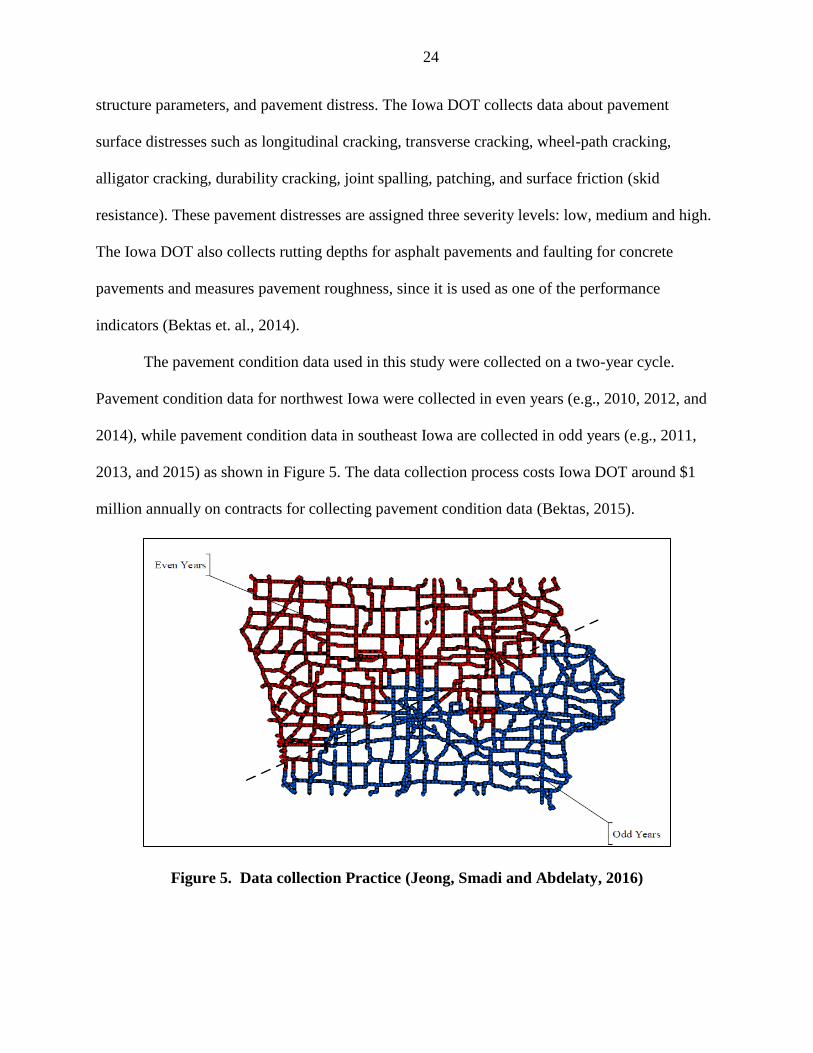
The pavement condition data used in this study were collected on a two-year cycle.
Pavement condition data for northwest Iowa were collected in even years (e.g., 2010, 2012, and
2014), while pavement condition data in southeast Iowa are collected in odd years (e.g., 2011,
2013, and 2015) as shown in Figure 5. The data collection process costs Iowa DOT around $1
million annually on contracts for collecting pavement condition data (Bektas, 2015).
Figure 5. Data collection Practice (Jeong, Smadi and Abdelaty, 2016)

25
The collected pavement condition data are aggregated into the PMIS database by
averaging the rutting and IRI values to represent the roughness and rutting of large pavement
sections and by counting the lengths of cracks to represent the length of cracks per unit length.
Each pavement section in the database includes IRI values, rutting depth, faulting values, and
surface distresses. Each section in the PMIS is defined by the route number, the county, the
highway system (Interstate, US, or Iowa highways), the direction, the district, and the beginning
and ending mileposts, as shown in Figure 6. The PMIS also contains traffic, material, layer
thicknesses, and pavement history information for each section. (Jeong et. al., 2016).
Figure 6. Screenshot from the PMIS database
Table 2 presents the total of directional miles for each of the seven pavement types in the
PMIS database in 2015.
In this research, only asphalt concrete cement (ACC), portland concrete cement (PCC),
and composite (COM) pavements were selected for developing performance prediction models
because there were insufficient miles for the other pavement types. ACC and PCC pavements are
described as flexible and rigid pavements, respectively.
Pavement condition data from 1998 through the end of 2015 was used in this research.
Each pavement section in the study had the same features (i.e., pavement type, maintenance
history, traffic loading, subgrade stiffness, layer thicknesses, and pavement distresses). Rutting,

26
roughness, faulting, longitudinal cracking, longitudinal wheel-path cracking, transverse cracking,
durability cracking, patching, and joint spalling were pavement distress features of the pavement
sections.
Table 2. Pavement types in Iowa highways
Pavement Types Directional
Miles % of Miles
ACC Asphalt concrete cement 1798.21 16.17%
PCC Portland concrete cement 3487.30 31.36%
COM Composite with asphalt surface 5156.81 46.38%
CRC w/ATB Continuous reinforcement concrete with
asphalt treated base
4.83 0.04%
CRC w/GSB or CTB Continuous reinforcement concrete with
granular or cement treated base
0.97 0.01%
Composite
w/JT PCC
Composite built on jointed concrete 262.23 2.36%
Composite w/CRC Composite built on continuous reinforcement
concrete
409.45 3.68%
Total 11119.80 100.00%
Iowa highways are classified into three systems: Interstate highways, US highways, and
Iowa highways. The most recent PMIS data from 2015 shows totals of approximately 460 miles
of interstate highway, 3544 miles of US highway, and 4567 miles of Iowa highway. The number
of miles of ACC, PCC, and COM pavements in interstate, US, and Iowa highways are given in
Table 3. The lengths and number of pavement segments at each pavement type based on 2015
data are given in Table 4.
Table 3. Center mile length of each pavement type (miles)
Pavement Type
ACC PCC COM Total
Interstate 57 364 39 460
Iowa 1366 752 2449 4567
US 221 1098 2225 3544
Total 1644 2214 4713 8571

27
Table 4. Descriptive statistics of pavement segments
Number of
Segments
Average Segment
Length (miles)
Minimum Segment
Length (miles)
Maximum Segment
Length (miles)
ACC 464 3.88 0.16 18.61
PCC 1200 2.70 0.05 18.91
COM 1920 2.69 0.05 18.14
Pavement Condition Indices
Four indices have been developed to evaluate the pavement conditions of Iowa highways.
These indices are on a 100-point scale to be consistent with the PCI scale that ranges from 0 to
100. Cracking and riding indices were developed for ACC, PCC, and COM pavements, rutting
indices were developed for ACC and COM pavements, and a faulting index was developed for
PCC pavements.
Cracking Index
Four types of cracking are evaluated by Iowa DOT for ACC pavements: transverse
cracking (count/mile), longitudinal cracking (ft/mile), longitudinal-wheel-path cracking (ft/mile),
and alligator cracking (ft2/mile). For PCC pavements, transverse cracking (count/mile),
longitudinal cracking (ft/mile), and longitudinal-wheel-path cracking (ft/mile) are evaluated.
The cracking index was developed based on a 100-point scale, with 0 indicating the worst
condition and 100 indicating the best condition. The cracking index includes sub-indices for each
type of crack. For instance, for ACC pavements, four sub-indices were developed for transverse,
longitudinal, longitudinal-wheel-path, and alligator cracking. For PCC pavements, two sub-
indices were developed for transverse and longitudinal cracking. Iowa DOT combines

28
longitudinal and longitudinal-wheel-path into one index since these show similar behavior in
PCC pavements.
These sub-indices are calculated based on deduction from 100 as shown in Equation 2,
𝐶𝑟𝑎𝑐𝑘 𝑆𝑢𝑏_𝑖𝑛𝑑𝑒𝑥 = 100 − (100 ×𝑐𝑟𝑎𝑐𝑘 𝑣𝑎𝑙𝑢𝑒
𝑡𝑟𝑒𝑠ℎ𝑜𝑙𝑑 𝑣𝑎𝑙𝑢𝑒) (2)
Iowa DOT has determined threshold values for calculating sub-indices for each pavement
type in Iowa highways as shown in Table 5 (Mark Murphy, personal communication, December,
2017).
Table 5. Threshold for cracking indices
Pavement Type
Cracking Type ACC PCC COM
Transverse (count/mile) 483 241 805
Longitudinal (ft/mile) 2640 1320 2640
Longitudinal-wheel-path (ft/mile) 2640 — 2640
Alligator (ft2/mile) 6236 — 6236
A cracking index for each pavement type was calculated by summing the weighted
coefficient values for ACC and COM and for PCC as shown in Equation 3 (for ACC and COM)
and 4 (for PCC). The coefficient values of each sub-index were determined by Iowa DOT using
equations 3 and 4.
𝐶𝑟𝑎𝑐𝑘 𝐼𝑛𝑑𝑒𝑥 (𝐴𝐶𝐶) = (0.2 × 𝑇𝑟𝑎𝑛𝑠𝑣𝑒𝑟𝑠𝑒) + (0.1 × 𝐿𝑜𝑛𝑔𝑖𝑡𝑢𝑑𝑖𝑛𝑎𝑙) + (0.3 × 𝐿𝑜𝑛𝑔𝑖𝑡𝑢𝑑𝑖𝑛𝑎𝑙𝑊𝑃) + (0.4 × 𝐴𝑙𝑙𝑖𝑔𝑎𝑡𝑜𝑟)
(3)
𝐶𝑟𝑎𝑐𝑘 𝐼𝑛𝑑𝑒𝑥 (𝑃𝐶𝐶) = (0.6 × 𝑇𝑟𝑎𝑛𝑠𝑣𝑒𝑟𝑠𝑒) + (0.4 × 𝐿𝑜𝑛𝑔𝑖𝑡𝑢𝑑𝑖𝑛𝑎𝑙) (4)
Riding Index
The Iowa DOT calculates the riding index by converting the IRI values using Equation 5:
𝑅𝑖𝑑𝑖𝑛𝑔 𝐼𝑛𝑑𝑒𝑥 = (𝐼𝑅𝐼 𝑣𝑎𝑙𝑢𝑒𝑠 −253
32−253) × 100 (5)

29
The riding index is a 100 scale, with 0 being the worst and 100 being perfect. On the Iowa DOT
ride index scale, all IRI values below 32 (in./mile) are considered to be 100, and all values above
253 (in./mile) are considered to be 0.
Rutting Index
Rutting depth is collected by Iowa DOT for ACC and COM pavements. Iowa DOT
converts the rutting depth values into a 100-point scale rutting index ranging from 0 (worst) to
100 (perfect) using Equation 6.
𝑅𝑢𝑡𝑡𝑖𝑛𝑔 𝐼𝑛𝑑𝑒𝑥 = 100 − ((𝑅𝑢𝑡𝑡𝑖𝑛𝑔 𝑑𝑒𝑝𝑡ℎ
0.47) × 100) (6)
Faulting Index
The faulting index is only calculated for PCC pavements (FIPCC) based on the fault
measurements from the PMIS database. The fault index also is a 100 scale where 100 indicates
the perfect condition (no faulting) and 0 the worst. The fault threshold value is 0.47 in. so values
equal to or greater than so 0.47 are rated as 0 on the faulting index. The Iowa DOT converts the
fault values into an index by using Equation 7.
𝐹𝑎𝑢𝑙𝑡𝑖𝑛𝑔 𝐼𝑛𝑑𝑒𝑥 = 100 − ((𝐹𝑎𝑢𝑙𝑡
0.47) × 100) (7)
Overall Pavement Condition Index
After calculating the individual indices, the overall pavement condition index (PCI) was
calculated by combining the weighted individual indices. The weighing factors were determined
by Iowa DOT. For PCC pavements, the PCI combines the cracking index, riding index, and
faulting index by weighting factors based on Equation 8. For ACC and COM pavements, the PCI
combines the cracking index, rutting index, and riding index as shown in Equation 9.
𝑃𝐶𝐼𝑃𝐶𝐶 = (0.4 × 𝐶𝑟𝑎𝑐𝑘𝑖𝑛𝑔 𝐼𝑛𝑑𝑒𝑥) + (0.4 × 𝑅𝑖𝑑𝑖𝑛𝑔 𝐼𝑛𝑑𝑒𝑥) + (0.2 × 𝐹𝑎𝑢𝑙𝑡𝑖𝑛𝑔 𝐼𝑛𝑑𝑒𝑥) (8)
𝑃𝐶𝐼𝐶𝑂𝑀 & 𝐴𝐶𝐶 = (0.4 × 𝐶𝑟𝑎𝑐𝑘𝑖𝑛𝑔 𝐼𝑛𝑑𝑒𝑥) + (0.4 × 𝑅𝑖𝑑𝑖𝑛𝑔 𝐼𝑛𝑑𝑒𝑥) + (0.2 × 𝑅𝑢𝑡𝑡𝑖𝑛𝑔 𝐼𝑛𝑑𝑒𝑥) (9)

30
Pavement Age
Pavement age, calculated as the difference between the PMIS year (input date) and either
the most recent resurfacing or construction year, affects pavement condition. In 2015, more than
60% of miles of Iowa highways were 40 years old or older, while more than 50% of interstate
and US highway miles were less than 30 years (Figure 7).
Figure 7. Distribution of pavement age of Iowa highway systems (2015)
Traffic Loading
Iowa highways carry heavy trucks, so traffic loading is a significant factor that might
cause pavement deterioration. The traffic loading data in the PMIS database contains the average
daily traffic (ADT); average daily truck traffic (Truck); and average equivalent single axle loads
(ESAL) (18,000 lb). The ESAL converts all traffic loading with different magnitude and axle
configuration into an equivalent number of 18,000 lb ESAL. Figure 8 shows the ESAL values
for the Interstate, US, and Iowa systems in 2015 in Iowa. and Figure 9 shows changes in traffic
loading over time.

31
Figure 8. Traffic loading distribution of Iowa highways (2015)
Figure 9. Changes in traffic loading on highways in Iowa
Climate Data
Weather conditions, such as temperature variation and moisture change, affect the
material properties of both pavement surfaces and sublayers (Žiliūtė et. al., 2016). Further, when
saturated pavement material is subjected to frost heave during freeze-thaw cycles freezing causes

32
tensile stresses that increase deterioration process (Smith et. al., 2006). Later thawing leaves
voids that can also contribute to pavement deterioration (Adkins et. al., 1989). The state of Iowa
is located in a wet-freeze climate zone and is exposed to severe weather, especially in the winter,
so it is important to investigate the effects of environmental factors on pavement condition,
particularly since weather factors have not previously been considered in pavement performance
modeling at the network level.
The climate data for this study was obtained from the Iowa Environmental Mesonet
(IEM). The IEM is a data collection project developed by the Department of Agronomy at Iowa
State University (ISU). The climate data in the IEM is based on observational data collected
from the National Weather Service (NWS) by manual and automated sensors in each county
across the state (Breakah et. al., 2010). The NWS is an agency in the United States that collects
all related information about weather conditions. In Iowa, there are 111 weather stations as of
2015 (Figure 10).
Figure 10. NWS climate stations in Iowa

33
The weather data that were used in the analysis were average annual temperature, average
annual rainfall, average annual snowfall, and the number of freeze-thaw cycles. Figure 11 shows
the format of the weather database that was obtained from the IEM at Iowa State University that
contains weather data from 1951 to the present.
Figure 11. Screenshot of the IEM weather database
Freeze-thaw cycles were defined by counting the number of times the temperature
changes from freezing to thawed states. In this research, the freeze-thaw cycle was considered
when the temperature fell below a freeze point (to be more conservative, 30°F was considered
the freeze point), and followed by the temperature rising above 32°F.
In some areas in Iowa, the number of freeze-thaw cycles was low because the
temperature stayed below 30°F all winter. For example, Figure 12 shows that the area in northern
Iowa had the fewest freeze-thaw cycles in 2014. Most freeze-thaw cycles happen during spring
and fall months when temperatures can be expected to change during a day.

34
Figure 12. Average annual freeze-thaw cycles for 2014
Data Integration
Geographic information system (GIS) software was used to integrate the PMIS road
condition data and the IEM climate data according to locations. The GIS spatial integration
process provided accurate overlays of the weather stations over Iowa highways. The GIS also
was used to display weather conditions as colored maps. To ensure that the climate data and
locations of each pavement section were associated, each pavement section was assigned to the
closest weather station. For example, Figure 13 shows the 32 pavement sections that were closest
to weather station IA0133.

35
Figure 13. Pavement sections associated with the closest weather station
The distances between the weather stations and their related pavement sections ranged
from 0 to 24 miles with an average distance of around 7 miles, while most pavement sections are
located between 0 and 5 miles from the weather station. Figure 14 shows the distribution of the
distances between pavement sections and their weather stations.
GIS software integrated the PMIS attribute table and weather station attribute table based
on their spatial locations to create the final dataset (Figure 15). In that dataset, that each
pavement section record contains the section location, pavement distresses, traffic loading, and
structural characteristics. Each pavement record also includes the average annual temperature,
snowfall and rainfall amount, the number of freeze-thaw cycles for the nearest weather station,
and the distance between each pavement segment and its closest weather station.

36
Figure 14. Distribution of the distances from pavement sections to the closest weather
station
Figure 15. Final dataset format after integration of PMIS and IEM data
After integrating the data for years from 1998 through 2015, the climate data (i.e.,
temperature, snowfall, rainfall, and freeze-thaw cycles) were represented by GIS maps to

37
illustrate which pavement segments had experienced more extreme conditions. Figure16 shows
the average annual temperature for the entire highway network in 2015, when the lowest average
was recorded in Worth County in northern Iowa. The highest average temperature in 2015 was
recorded in Polk County in the middle of the state around Des Moines.
Figure 16. Iowa average temperatures (2015)
The statewide average annual rainfall was higher in the southern part of the state (Figure
17) in 2015 when he largest amount of rain fell on Taylor County in southern Iowa. The
statewide average annual snowfall in 2015 was highest in northern Iowa.

38
Figure 17. Average rainfall amount (in.) on Iowa highways (2015)
Figure 18 shows the higher amount of snow was in Clayton County in the northwest part
of the state. Figure 19 illustrates the number of freeze-thaw cycles over the state when
temperatures fluctuated above and below freezing. In 2015, the most freeze-thaw cycles occurred
in the southern and western parts of the state.

39
Figure 18. Average snowfall amount (in.) on Iowa highways (2015)
Figure 19. Number of freeze-thaw cycles of Iowa highways (2015)
40
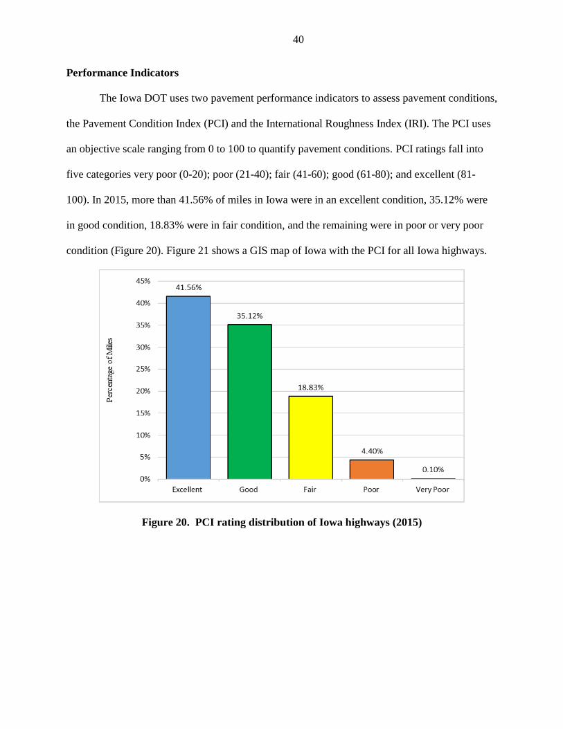
Performance Indicators
The Iowa DOT uses two pavement performance indicators to assess pavement conditions,
the Pavement Condition Index (PCI) and the International Roughness Index (IRI). The PCI uses
an objective scale ranging from 0 to 100 to quantify pavement conditions. PCI ratings fall into
five categories very poor (0-20); poor (21-40); fair (41-60); good (61-80); and excellent (81-
100). In 2015, more than 41.56% of miles in Iowa were in an excellent condition, 35.12% were
in good condition, 18.83% were in fair condition, and the remaining were in poor or very poor
condition (Figure 20). Figure 21 shows a GIS map of Iowa with the PCI for all Iowa highways.
Figure 20. PCI rating distribution of Iowa highways (2015)

41
Figure 21. PCI map of Iowa highways (2015)
The International Roughness Index (IRI) is obtained by measuring the longitudinal profile of a
pavement. Pavements are classified as good (95 in./mile); fair (95–170 in./mile); or poor (>170
in./mile) condition. In 2015 in Iowa, 52.66% of highway miles were in good condition, 39%
were in fair condition, and 8.31 % were in poor condition (Figure 22). Figure 23 is a map of the
IRI measurements of Iowa highways in 2015.

42
Figure 22. Pavement roughness distribution of Iowa highways (2015)
Figure 23. IRI map of Iowa highways (2015)

43
Developing Pavement Performance Models
Two kinds of pavement performance models, traditional multiple linear regression
(MLR) and artificial neural network (ANN) models were developed to study three pavement
types with different pavement properties and different material properties. Goodness of fit is a
common measure for evaluating model performance. Therefore, the coefficient of determination
(R2) and root mean square error (RMSE) were utilized to measure and compare the performance
of the models. Good prediction models should have a high R2 and a low RMSE. R2 values
represent the correlation between the actual and predicted values to determine the accuracy of the
model (Rahman and Tardfer, 2017). R2 values range between 0 and 1 where 1 indicates that the
actual and predicted values are in agreement and 0 indicates there is no relationship between
them. RMSE values represent used measure the differences between predicted and actual values.
R2 and RMSE values were determined using Equation 10 and Equation 11 respectively
n
i
i
n
i
ii
yy
yy
R
1
2
1
2
2
ˆ
1
(10)
n
yy
RMSE
n
i
ii
2ˆ
(11)
where
𝑦𝑖 = actual value observation i;
�̂� = predicted value of observation i;
�̅� = average value of observation i; and
n = number of observations.
Historical data was used on in both ANN and MLR models to predict individual
distresses for three pavement types, ACC, PCC, and COM pavements. These individual

44
distresses were predicted based on weather factors (i.e., temperature, precipitation, and freeze-
thaw cycles), traffic loading, pavement age, SN, layer thicknesses, and subgrade stiffness. By
predicting individual distresses, decision makers can evaluate the individual distress for each
pavement section, and determine which distress has more effect on the overall pavement
condition.
These models were used to predict the individual distresses in ACC, PCC, and COM
pavements. For ACC and COM pavements, three models were developed for predicting
roughness, cracking, and rutting, and for PCC pavements, three models were developed for
predicting roughness, cracking, and faulting. These predicted distresses were combined to
calculate the PCI values based on Equations 8 and 9 in order to represent the overall PCI over the
years. The flowchart in Figure 24 illustrates the modeling process. To determine the reliability of
ANN models, the results obtained from the ANN models were compared with the results from
MLR models.
Figure 24. Flowchart of predicting PCI for ACC pavements
Stepwise analysis was used to determine factors that affect pavement conditions to
remove any correlation between input variables by using JMP software. Stepwise analysis is the

45
best approach for selecting candidate variables and removing insignificant variables (Nunez, et.
al., 1986). In general, the factors that affect pavement conditions are climate factors (i.e.,
temperature, rainfall, snowfall, and freeze-thaw cycles), traffic loading, pavement thickness,
structure number, and initial measurement values of pavement conditions.
The initial values of pavement conditions have been used by researchers as input factors
to predict pavement conditions. Wang and Li (2011) predicted pavement roughness based on the
initial roughness values, and Evangelista et. al., (2012) reported that initial crack size and
pavement thickness have a significant impact on increasing the crack growth rate in concrete
pavements. Smith et. al. (2002) reported that predicting the riding index will be improved
significantly when initial roughness is considered. However, for this study, at the network level,
the initial conditions of pavement sections were not available in the PMIS database. Iowa DOT
collects pavement condition data in two year cycles, and the most recent measurement values are
used as initial values in this study. This approach of using previous pavement condition values
has been used by Kargah-Ostadi et. al. (2014) who considered the most recent IRI value instead
of the initial, constructed IRI value to predict pavement roughness. Also, Meegoda and Gao
(2014) reported that IRI data from previous years can be used as an initial IRI value when initial,
constructed roughness data is not available. The input variables used in this study to predict the
riding, cracking, and rutting indices for ACC, COM, PCC pavements are listed in Tables 6, 7,
and 8, respectively.

46
Table 6. Input variables for modeling ACC pavements
Riding Index (RI) Cracking Index (CI) Rutting Index (RuI)
Pavement age
Previous RI value
Pavement thickness
Subgrade stiffness
Average rainfall
Average temperature
Pavement age
Previous CI value
Average temperature
Structure number
Pavement age
Previous RuI value
Pavement thickness
Average temperature
Table 7. Input variables for modeling COM pavements
Riding Index (RI) Cracking Index (CI) Rutting Index (RuI)
Pavement age
Previous RI value
PCC thickness
Pavement thickness
Subgrade stiffness
AADT
Average temperature
Average rainfall
Freeze-thaw cycles
Pavement age
Previous CI value
ACC thickness
PCC thickness
Subgrade stiffness
Trucks
Average temperature
Pavement age
Previous RI value
PCC thickness
Pavement thickness
Subgrade stiffness
AADT
Structure Number
Average temperature
Average snowfall
Average rainfall
Freeze-thaw cycles
Table 8. Input variables for modeling PCC pavements
Riding Index (RI) Cracking Index (CI) Faulting Index (FI)
Pavement age
Previous RI value
Average rainfall
Freeze-thaw cycles
Pavement age
Previous CI value
Trucks
Pavement thickness
Pavement age
Previous FI value
AADT
Average rainfall
Freeze-thaw cycles
Before analyzing the data, JMP software was used to randomly divide the dataset into a
training dataset (70%) and a validation dataset (30%) to explain how well the model performed.
The performance of the prediction models was evaluated using two approaches: root mean
square error (RMSE) and coefficient of determination (R2).

47
Developing Artificial Neural Network (ANN) Models
Three main components are used to develop ANN models: the structure of connection
between input and output layers (architecture); the method of adjusting the connection weight
(learning method); and the neuron activation function.
ANN architecture plays a major role in developing an optimum ANN model, and efforts
are required to determine the optimum architecture. The ANN model architecture used in this
study consists of three layers: input layer, hidden layer, and output layer as shown in Figure 25.
At the input layer, the independent variables that relate to the output layer are entered,
and each independent variable is assigned to an individual neuron. The challenge is to decide
how many neurons should be in the hidden layer because that choice impacts model
performance. For example, using too many neurons in a hidden layer might make the model
more complex (Rafiq et. al., 2001).
Figure 25. Neural network architecture (Yang, Lu, and Gunaratne, 2003)

48
There is no standard method for selecting the appropriate number of neurons, so training
the ANN model with sequential number of hidden neurons and then selecting the number of
neurons that achieve minimum RMSE was employed. Figure 26 shows the performance of an
ANN model for determining the number of neurons in the hidden layer for predicting cracking
index in composite pavement where the lowest RMSE value was achieved at 12 hidden neurons.
The final layer in the structure of ANN model is the output layer that produces the result from
processing provided by the hidden layer.
Figure 26. RMSE values to determine the number of neurons for training a COM
pavement model
ANN learning process
After determining the architecture of an ANN model, software (e.g., JMP) is used to
randomly divide the database is into training (70%) and validation (30%) datasets to train the
neural networks. The training data set is used to develop the model, while the validation data is
used to assess the accuracy of the ANN model and avoid overfitting in the model (Ling et. al.,

49
2017). The results of the training process produce the weight matrices that are stored in links
between layers and that can also be used to extract information about the contribution of each
input in the model output. In the training process, the connection weights between the layers is
adjusted, thereby, minimize the overall mean error by using back-propagation algorithm.
In general, the ANN learning process is usually classified into supervised and
unsupervised processes (Shahin et. al., 2008). The supervised learning process utilizes historical
data both for network inputs and desired outputs. The predicted output is compared to measured
values to calculate an error that can then be used to adjust the connection weights between the
model inputs and outputs. In the unsupervised learning process, the connection weight is
adjusted based on stimuli inputs with no desired output provided in order to cluster the input
values to similar features.
The back-propagation algorithm is considered as a supervised learning process, and it has
been adopted by most researchers (Zhang et. al., 1998). In back-propagation algorithm, the input
data propagated to the neurons in the hidden layer for processing, after which, the resulting data
are propagated to the output layer. The results from the output layer are compared to the actual
data for calculating the resulted error, following which the weights are adjusted after the
calculated error is propagated back, with the process repeated until the model produces a lower
error value.
Neuron activation function
The basic unit of an ANN model is a neuron that combines inputs and produces an output
as shown in Figure 27. The neurons are not individually powerful in terms of computational
power, but their interconnection with neurons in different layers produces the desired
relationship among variables and demonstrates the processing capabilities of the neurons (Attoh-
Okine, 1994).

50
Figure 27. Diagram of an artificial neuron (Liu, 2013)
Each neuron in the hidden layer has its own summation and transfer functions with
respect to the input and output values. The activation function determines the relationship
between inputs and output layers. The output of the summation function is given by Equation 11,
n
i
iij wxfOy1 (11)
where:
Oj = output of hidden neuron jth;
f = transfer function
xi = ith input; and
wi: connection weight between input ith and output jth.
Five transfer functions: linear, linear threshold, step, sigmoid and Gaussian functions
have been used in a number of studies depending on the characteristics of the problem under
investigation (Liu, 2013). The sigmoid function has been used in this research as the neuron
activation function because of its support of nonlinearity and capability for avoiding excessively
large values. The sigmoid transfer function is presented in Equation 12,

51
eya
yf)(
1
1)(
(12)
where
y = input to the transfer function; and
a = coefficient of sigmoid function.
Relative contribution of input variables
Despite the vast capability of ANN in prediction modeling, such models are often
criticized as “black box” models, because of the difficulty in interpreting the contribution of each
variable to the response variable making it hard to gain an understanding of the relationships
among variables, which is considered a weakness when compared to traditional statistical models
(Olden and Jackson, 2002).
In ANN models, the values of weights links between input, hidden, and output layers
play a significant role in determining the relative contribution of independent variables.
Shekharan (1999) reported that a number of researchers have attempted to extract the knowledge
of an ANN model by utilizing the connection weights to estimate the relative importance of each
variable from information stored in the weights. The common approach for estimating the
relative importance of different input variables in pavement performance prediction models is
called Garson’s algorithm. Garson’s algorithm has been found to produce more reliable results in
the case of nonlinear relations (Fischer, 2015). In Garson’s algorithm, the output layer
connection weight is partitioned into each input neuron using the absolute value of connection
weights (Olden and Jackson 2002). Shekharan (1999) presented the equation that has been
utilized to calculate the relative contribution of each independent variable in ANN models
(Equation 13),

52
v
i
h
jv
i
ij
jij
h
jv
i
ij
jij
w
Ow
w
Ow
RC
(13)
where:
h = number of hidden neurons
v = number of input variables
jO = connection weight between (j) hidden neurons and the output neuron
𝑤𝑖𝑗 = connection weight values between inputs (i) and (j) hidden neurons
Garson’s algorithm was utilized to calculate the relative contribution (RC) of independent
variables. RC values range between 0 and 100 percent, where the larger RC of a specific factor
indicates that it has a greater effect on the pavement condition. RC values were calculated for the
effects of variables on riding, cracking, rutting, and faulting for ACC, PCC, and COM
pavements.
Developing Multiple Linear Regression (MLR) Models
Regression analysis is a powerful method that requires historical data to predict a
dependent variable based on one or more independent variables. In this research, multiple linear
regression (MLR) models were used to predict values of pavement conditions (ride, cracking,
rutting, and faulting) and those results were compared with prediction results from ANN
modeling. MLR modeling has been widely used by highway agencies to predict pavement
performance because of its simplicity and ease of implementation. MLR has also been used by
researchers in predicting pavement deterioration rates (Xu et. al., 2015). Knapp et. al. (2000)
developed an MLR model to investigate the effect of winter weather on traffic volume and safety
in roads.
Some regression assumptions must be considered in developing regression models. For
example, Sousa et. al. (2007) reported that error values are assumed to be independent across

53
observations because collinearity between variables can lead to incorrect predictions. Smith et.
al., (1999) reported that the distribution of the error term is a normal distribution 𝑁(0, 𝜎2) and
that the relationship between response variable (yi) and the explanatory variables is linear
(Equation 14),
𝑌 = 𝛽0 + 𝛽𝑋 + 𝑒 (14)
where
Y = dependent (response) variable;
𝛽𝑜 = constant term;
𝛽 = regression coefficient;
𝑋 = independent variable; and
𝑒 = error term.
An ANN Model for Correlating Structural Capacity and Rutting
Several factors such as climate factors, thickness, and traffic loading cause rutting in
ACC pavements (Mirzapour Mounes et. al., 2014). An ANN model was developed for this study
to estimate the correlation between structural capacity and rutting. Traffic loading, pavement
age, subgrade stiffness, layer thickness, average annual number of snowfall, average annual of
rainfall, average annual temperature, freeze-thaw cycles, and rutting were utilized as independent
variables to predict the structure number (SN). SN represents the pavement structural capacity
and was used as the dependent variable.
The analysis process focused on ACC pavements on Iowa highways. The other pavement
types were not included in this analysis because there was insufficient structural data for those
cases. Also, the analysis focused on ACC pavement sections that have not been exposed to any
maintenance or rehabilitation activities. So the obtained data includes all section data until the
year of applying any maintenance or rehabilitation operations.
A total of 1144 data points from Iowa highways for years from 1998 to 2015 were trained
by using the back-propagation algorithm ANN model. Before training the ANN model, JMP

54
software divided the dataset randomly into 70% for training process and 30% for the validation
process. The performance of the ANN model was evaluated by coefficient of determination (R2)
and root mean square error (RMSE).

55
CHAPTER 4: RESULTS AND DISCUSSION
Understanding pavement performance during its service life has an impact on managing
the roads in an effective manner and optimizing maintenance and rehabilitation strategies. This
chapter presents the results of utilizing ANN and MLR models with both pavement condition
and weather variables to predict pavement performance conditions. Future pavement conditions
of Iowa highways were predicted more accurately by ANN models than MLR models. The ANN
model demonstrated the capability for predicting pavement conditions based on several variables
and for estimating the relationship between SN and rutting in asphalt pavements at the network
management level.
Comparison of ANN and MLR Models
The performance of the ANN models was compared with the performance of the MLR
models to assess the accuracy of the models in predicting pavement performance as calculated by
riding, rutting, cracking, and faulting indices. R2 and RMSE values were used to measure and
compare the performance of the models. Good prediction models should have a high R2 and a
low RMSE.
Historical data was used on both ANN and MLR models to predict individual distresses
for three pavement types, ACC, PCC, and COM pavements. These individual distresses were
predicted based on weather factors (i.e., temperature, precipitation, and freeze-thaw cycles),
traffic loading, pavement age, SN, layer thicknesses, and subgrade stiffness. By predicting
individual distresses, decision makers can evaluate the individual distress for each pavement
section, and determine which distress has more effect on the overall pavement condition.
After determining the architecture of each ANN model, the database for the period from
1998 to 2015 was randomly divided by JMP software into training (70%) and validation (30%)

56
datasets. JMP software was also used for training the neural networks. The training data set was
used to develop the model whereas the validation data was used to assess the accuracy of the
ANN model and avoid overfitting in the model (Ling et. al., 2017). The results of the training
process produced the weight matrices that are stored in links between layers and that can also be
used to extract information about the contribution of each input in the model output. The analysis
showed that the ANN models yield reasonably accurate models compared to the results of MLR
models as shown in Tables 9, 10, and11.
For ACC pavements, the ANN models yielded more accurate predictions than the MLR
models in riding, cracking, and rutting indices as shown in Table 9. The R2 values indicate there
are good correlations between actual and predicted indices for each index. The R2 values from
the ANN models are higher than the R2 values of the MLR models by 61.40%, 48.15%, and
48.15% for riding, cracking, and rutting index, respectively.
Table 9. Comparison of MLR and ANN for ACC pavements
Pavement Index MLR ANN % of R2 Improvement
R2 RMSE R2 RMSE
Riding Index 0.57 12.97 0.92 8.42 61.40%
Cracking Index 0.54 16.62 0.80 14.31 48.15%
Rutting Index 0.41 12.10 0.72 9.16 75.61%
For PCC pavements, as can be seen in Table 10, the ANN models achieve better accuracy
models with improvement in R2 by 23.00%, 26.93%, and 80.00% than MLR models in
predicting riding, crack, and fault indices, respectively, compared with MLR models.

57
Table 10. Comparison of MLR and ANN for PCC pavements
Pavement Index MLR ANN % of R2 Improvement
R2 RMSE R2 RMSE
Riding Index 0.74 11.84 0.91 10.60 23.00%
Cracking Index 0.54 18.61 0.68 15.23 26.93%
Faulting Index 0.35 15.00 0.63 12.96 80.00%
For COM pavements, the comparison of the results produced by ANN and MLR models
showed that the ANN model performed better accurate models than MLR models as shown in
Table 11. The R2 values from the ANN models indicate that the ANN models are more accurate
than MLR models.
Table 11. Comparison of MLR and ANN for composite pavements
Pavement Index MLR ANN % of R2 Improvement
R2 RMSE R2 RMSE
Riding Index 0.54 15.68 0.88 11.72 62.96%
Cracking Index 0.65 14.00 0.88 13.50 35.38%
Faulting Index 0.44 12.57 0.75 9.78 70.45%
These analyses show that the ANN model is more accurate than the MLR model. This
conclusion is consistent with conclusions reported in previous studies. For example, Chandra, et.
al. (2012) compared between the performance of ANN and MLR models in predicting pavement
roughness from different kinds of distress and reported that the ANN model has significantly
better accuracy than MLR model with mean square error 18% less than that for the MLR. These
findings are consistent with Thube (2012) who developed ANN models to predict cracking,
raveling, rutting and roughness and reported good R2 values. Saghafi et. al. (2009) also reported
that the ANN models predicted faulting in concrete pavement with higher accuracy than an MLR
model. In this research, both the ANN and MLR models included the weather factors that
influence pavement conditions.

58
Validation of Prediction Models
For the ANN models, the process of developing the neural network of a validation dataset
is similar to the training process, except no weight matrices are produced from the validation
process. If the accuracy of models from the validation process is higher that indicates the
prediction model perform well (Ling et. al., 2017). Otherwise, the model needs to be run with
different architecture until it gets similar error values for training and validation datasets. In this
study, the R2 values from the validation process of the ANN models ranged from 0.60 to 0.91,
while RMSE values ranged from 19.22 to 8.69 (Table 12).
Table 12. Goodness of fit of ANN models of validation dataset
Pavement Type Pavement Index R2 RMSE
ACC
Riding Index 0.91 8.69
Cracking Index 0.78 14.68
Rutting Index 0.70 9.67
PCC
Riding Index 0.90 11.73
Cracking Index 0.67 19.22
Faulting Index 0.60 13.53
COM
Riding Index 0.87 12.06
Cracking Index 0.81 14.00
Rutting Index 0.74 9.97
For the MLR models, residual plots were used to assess the performance of the MLR
model. The residual is the difference between predicted and measured values and is calculated by
Equation 15.
ei = actual i – predicted i (15)
The analysis of residual distribution plots is the most common technique used to verify
that regression assumptions were met (Rajagopal, 2006). The residual plots for the MLR models
were approximately randomly distributed around the centerline at 0 with no certain pattern. This
indicates that the MLR models successfully predicted the dependent variables and that the
constant variance assumption was verified. Figures 28, 29 and 30 show the residual plots of the

59
performance prediction models of cracking, riding, and rutting indices in ACC pavements,
respectively.
Figure 28. Residual plot for the cracking model in ACC pavements
Figure 29. Residual plot for the riding model in ACC pavements
Figure 30. Residual plot for the rutting model in ACC pavements

60
ANN Predictions of Future Pavement Performance
After predicting the pavement condition indices, the weights and biases matrices from
ANN layers were used to predict the future performance of riding, cracking, rutting, and faulting
indices assuming no future treatment will be applied. The adjusted weights were developed by a
back-propagation algorithm during the training process in order to make the predicted values
close to the actual values. The weights and biases matrices were stored by JMP software.
Predicting the future pavement conditions was predicted incrementally; for instance, the first
predicted value for pavement condition in age (t+1) was used to predict the second year
pavement condition (t+2) as the input of the previous pavement condition and so on. The ANN
models were based on the average of weather factors and traffic loading, structure parameters,
and initial pavement condition. Thereafter, these values from each distress index were combined
together to present PCI values calculated using Equation 8 (for ACC and COM) and Equation 9
(for PCC) pavements. These PCI values provide performance predictions for the three kinds of
pavement.
Performance curves were drawn between PCI and pavement age. The ultimate goal of the
performance curves is to effectively assist decision makers in knowing when, where, and what
maintenance action should be taken for a given pavement section based on PCI values. The PCI
scale is divided into very poor, poor, fair, good, and excellent conditions based on threshold
values on a scale that ranges from 0 to 100 (Table 13).
Table 13. Threshold values of PCI from Iowa DOT
PCI Interstate highway
Very Poor 0–20
Poor 21–40
Fair 41–60
Good 61–80
Excellent 81–100

61
ANN models were used to predict the pavement performance of ACC, PCC, and COM
pavements during their design life period. For this analysis, three pavement sections, one each of
ACC, PCC, and COM pavements, were selected to analyze their performance over the years and
predict future performance. The curves for each pavement section begin at the year of
construction, and it is assumed that no maintenance has been or will be done on the section.
These curves are shown in Figures 31, 32, and 33.
ACC pavements represent about 16% of Iowa highways. The performance curve for an
ACC pavement section from I-35 is shown in Figure 31. The performance curve shows that the
pavement section was in poor condition, (i.e., the PCI value is lower than 41) 11 years after
construction.
Figure 31. Pavement performance curve for I-35 section (ACC pavement)

62
Figure 32 shows the performance curve of a pavement section of US-30 in Story County.
The pavement type of this section is a composite pavement with PCC overlaid by ACC
pavement. Composite pavement is widely used in Iowa, with around 46% of the total highway.
The composite pavements typically last longer than ACC pavement because the concrete base
layer makes it a stronger structure. The US-30 pavement section can serve in good or fair
condition up to approximately 20 years, which is better performance than the ACC pavement
section.
Figure 32. Pavement performance curve for US-30 section (COM pavement)
Figure 33 shows the performance curve of a PCC pavement section of Iowa highway 1.
This performance curve indicates that PCC pavement lasts longer than both ACC and COM
pavements and that PCC deteriorates at a lower rate early age. The curve indicates that this
pavement section should be in good or fair condition for almost 40 years.

63
Figure 33. Performance curve for the Iowa-1 pavement section (PCC pavement)
Relative Contribution of Input Variables
An effort has been made in this study to estimate the relative importance of each input
variable in predicting the individual distress values for each pavement type. By knowing the
relative contribution of each variable in the ANN models, the image of ANN as black box model
can be changed. Garson’s algorithm (Equation 13) utilizes connection weights in links between
ANN layers to calculate the relative contributions (RC) of input variables (e.g., temperature or
traffic loading) on output variables (e.g., rutting or cracking). The RC of each input variable is
reported as a percentage, with the total RC equal to 100%. Because pavement types are not
necessarily influenced by every input variable, only the variables that influence the indices
related to each pavement type are shown.

64
Variables that Influence ACC Pavements
Figures 34 through 36 show the relative contribution of input variables on the riding,
cracking, and rutting indices values for ACC pavements. The pavement age was the most
significant factor affecting the riding index. The significance of age in predicting riding indices
in ACC, PCC, and COM pavements was expected because increasing pavement age means
increased exposure to weather factors and traffic loads. Also, pavement age is considered the
best predictor because it can be determined accurately. The average annual temperature has a
large influence on riding, cracking, and rutting indices, which is consistent with previous studies.
The cracking and rutting and indices were significantly affected by weather temperature (Figures
34 and 35).
These results are consistent with previous research, such as a study done in Michigan that
reported that the performance of flexible pavements is most sensitive to temperature and
precipitation (Yang et al., 2017). Also, Breakah et al. reported that for ACC pavement, high
temperature affects the resilient modulus of pavements, cold weather increases pavement
stiffness, which can cause shrinkage cracking, and precipitation possibly affects the strength of
the subgrade by infiltration through layers (2010). Temperature variation can reduce the strength
of asphalt surface layers and cause rutting, which means the pavement structure cannot carry the
expected traffic loads (Johanneck and Khazanovich, 2010).

65
Figure 34. Relative contribution of inputs on Riding Index (ACC Pavement)
Figure 35. Relative contribution of inputs on Cracking Index (ACC Pavement)

66
Figure 36. Relative contribution of inputs on Rutting Index (ACC Pavement)
Variables that Influence PCC Pavements
For PCC pavement, as shown in Figure 37, the riding index is greatly affected by the
previous roughness value, and this finding was shown in literature reviews. According to a study
done in Wisconsin, the previous roughness value has a large impact on predicting pavement
roughness in concrete pavements (Wen and Chen, 2007). Also, pavement age affects both riding
and cracking indices of PCC pavements because as pavement age increases, the ability of a
concrete slab to withstand repeated traffic loadings and weather factors decreases.
The relative contributions of rainfall and freeze-thaw cycles were of secondary
importance after previous values of IRI and pavement age, but collectively their contributions
reach 20% (Figure 37). However, weather factors have a higher influence on predicting the
faulting index. The largest effect on the faulting index comes from temperature with a relative
contribution around 50% (Figure 38). The effect of temperature on concrete pavement has been
found in previous research. For example, curling and warping of concrete pavement slab are

67
caused by temperature variation (Johanneck and Khazanovich, 2010). Truck loadings on PCC
pavements also contribute nearly 60% to predicting the cracking index (Figure 39).
Figure 37. Relative contribution of inputs on Riding Index (PCC Pavement)
Figure 38. Relative contribution of inputs on Faulting Index (PCC Pavement)

68
Figure 39. Relative contribution of inputs on Cracking Index (PCC Pavement)
Variables that Influence Composite Pavements
For COM pavement, Figure 40 shows the factors that have an effect on riding index
values. Since COM pavements are constructed with a PCC base layer under an ACC, factors that
affect riding index in ACC and PCC pavements were found to have significant influence on the
riding index of COM pavement. The riding index was most affected by freeze-thaw cycles
whereas the cracking index was affected by average annual temperatures as shown in Figures 40
and 41. According to Chen et. al. (2015), freeze-thaw cycles can cause cracking, especially
reflective cracking in the PCC layer by movements at slab joints. The average number of freeze-
thaw cycles, the average annual temperature, and the average annual snowfall amount were
found to have a large impact on the rutting index (Figure 42). The results show that COM
pavements were less sensitive to traffic loading because combining PCC and ACC results in
good structural capacity.

69
Figure 40. Relative contribution of inputs on Riding Index (COM Pavement)
Figure 41. Relative contribution of inputs on Cracking Index (COM Pavement)

70
Figure 42. Relative contribution of inputs on Rutting Index (COM Pavement)
The main contribution of this research is to evaluate and quantify the impact of weather
factors on pavement conditions of ACC, PCC, and COM pavements. Considering weather
factors is important in modeling pavement performance, because pavement deterioration rates in
Iowa are definitely affected by freeze-thaw cycles, temperatures, and precipitation. These results
can be used by decision makers and maintenance engineers to determine proper treatment actions
and improve pavement design to withstand harsh weather over the years.
ANN Models for Correlating Structural Capacity and Rutting
Before training the ANN model to investigate the relationship between the SN and rutting
depth, the two were plotted to determine any relationship between them. Figure 43 shows that
there is no strong relationship between the actual rutting depth and the actual SN.
Different combinations of neural network architecture were examined to develop the best
ANN model for correlating SN and rutting depth in ACC pavements in Iowa. Applying an ANN
model with pavement thickness, subgrade stiffness, traffic loading, pavement age, temperature,
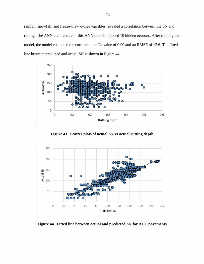
71
rainfall, snowfall, and freeze-thaw cycles variables revealed a correlation between the SN and
rutting. The ANN architecture of this ANN model included 10 hidden neurons. After training the
model, the model estimated the correlation an R2 value of 0.90 and an RMSE of 12.6. The fitted
line between predicted and actual SN is shown in Figure 44.
Figure 43. Scatter plots of actual SN vs actual rutting depth
Figure 44. Fitted line between actual and predicted SN for ACC pavements

72
These results demonstrate that ANN modeling can use rutting data to estimate the
structural capacity of an ACC pavement. In general, structural evaluation tests (e.g., deflection
testing) should be used to directly assess pavement structures. However, when there is no
structural data available, rutting data can analyzed to provide an estimation of SN.

73
CHAPTER 5: CONCLUSIONS AND RECOMMENDATIONS
Predicting future pavement performance is essential for allocating available funding for
maintenance and rehabilitation activities at the network level as well as for determining the most
cost-effective strategies at the project management level. The objectives of this study were to use
ANN models to accurately predict pavement performance of ACC, PCC, and COM pavements in
Iowa and to estimate the correlation between structural capacity (SN) and rutting depth on ACC
pavements.
The models in this study were developed to include climate data in addition to historical
pavement condition data. This research included weather factors as inputs in both ANN and
MLR prediction models. Results of the ANN models were more accurate than the MLR models,
perhaps because ANN models can deal with larger, more complex data sets. It is important to
determine the relative contribution of each factor to consider them in future design adjustments
and selecting appropriate treatments. Also, by identifying factors affecting pavement
performance, the idea about a neural network model as a black box model can be changed. Four
weather factors were included: average annual temperature, average annual snowfall, average
annual rainfall, and freeze-thaw cycles. The average annual temperature influenced the
performance of ACC pavements. Cracking, riding, and rutting distresses in ACC pavements
were impacted by temperature. Furthermore, the average annual temperature, freeze-thaw cycles,
and precipitations affected distress in COM pavements. The PCC pavements were most sensitive
to temperature, snowfall, and freeze-thaw cycles on the faulting index whereas the cracking
index was affected by truck loadings and pavement age. The riding index in PCC pavements was
mostly impacted by previous riding index values and pavement age.

74
ANN modeling of ACC pavements based on historical data that included structural
characteristics, traffic, weather, and pavement age also provided clear evidence of the
relationship between rutting and structural capacity. The model accurately estimated the
correlation between structural performance using rutting data for ACC at the network level.
Because conducting deflection tests to determine structural capacity is expensive and extensive
experience and knowledge is required to deal with the resulting data, this research suggests that
an ANN approach might be feasible for small transportation agencies (cities and counties) to
assess the strength of asphalt pavements.
This research developed models that accurately predicted future pavement conditions,
predictions that can support decisions for pavement maintenance activities and resource
allocation in pavement management systems.
This research recommends to determine the impact of the changes in pavement
deterioration resulting from weather data on the decision support tools used by Iowa DOT such
as allocating available fund, and that the Iowa DOT would improve the pavement management
system. Further, it is recommended that Iowa DOT consider adopting ANN pavement
performance modeling that includes pavement condition and weather variables to support
decisions at both the network and project management levels. Further research effort can also
focused on calibrating the mechanistic empirical pavement design guide performance models
based on the ANN results
This research had some limitations related to pavement distress data and climate data. Over 40% of
the Iowa DOT pavement are composite and the cracking data did not address reflective cracking.
Adding reflective cracking could help further refine the accuracy of the performance models.

75
Regarding weather data, in some cases, weather stations were 24 miles and that might not have been
reflective of the local conditions.

76
REFERENCES
AASHTO. (1993). AASHTO guide for design of pavement structures. 1993 (Vol. 1). AASHTO.
AASHTO. (2012). Pavement management guide. 2012. (2nd ed.). AASHTO.
Abdel-Khalek, A. M., M. A. Elseifi, K. Gaspard, Z. Zhang, & K. Dasari. (2012). Model to
Estimate Pavement Structural Number at Network Level with Rolling Wheel
Deflectometer Data. Transportation Research Record: Journal of the Transportation
Research Board, (2304), 142-149.
Adeli, H. (2001). Neural networks in civil engineering: 1989–2000. Computer-Aided Civil and
Infrastructure Engineering, 16(2), 126-142.
Adkins, D. F., & V. T. Christiansen. (1989). Freeze-thaw deterioration of concrete
pavements. Journal of Materials in Civil Engineering, 1(2), 97-104.
Archilla, A. R., & S. Madanat. (2000). Development of a pavement rutting model from
experimental data. Journal of Transportation engineering, 126(4), 291-299.
ASCE. (2015). Iowa infrastructure 2015 report card. American Society of Civil Engineers.
Attoh-Okine, N. (1994). Predicting roughness progression in flexible pavements using artificial
neural networks. Transportation Research Board Conference Proceedings, (Vol. 1,
No. 1).
Attoh-Okine, N., & O. Adarkwa. (2013). Pavement condition surveys—Overview of current
practices. Delaware Center for Transportation, University of Delaware: Newark, DE,
USA.
Ayed, A. (2016). Development of empirical and mechanistic empirical performance models at
project and network levels. (Doctoral thesis, University of Waterloo, Waterloo, Ontario,
Canada). Retrieved from https://uwspace.uwaterloo.ca/handle/10012/10606.
Basheer, I. A., & M. Hajmeer. (2000). Artificial neural networks: Fundamentals, computing,
design, and application. Journal of Microbiological Methods, 43(1), 3-31.
Bektas, F., O. Smadi, & M. AL-Zoubi. (2014). Pavement management performance modeling:
Evaluating the existing PCI equations. Iowa State University, Institute of Transportation.
Bektas, F., O. Smadi, & I. Nlenanya. (2015). Pavement condition: New approach for Iowa
Department of Transportation. Transportation Research Record: Journal of the
Transportation Research Board, (2523), 40-46. https://doi.org/10.3141/2523-05
Breakah, T., R. C. Williams, D. E. Herzamann, & E. S. Takle. (2010). Effects of using accurate
climatic conditions for mechanistic-empirical pavement design. Journal of
Transportation Engineering, 137(1), 84-90.
BTS. (2012). U.S. Department of Transportation. 2012 Commodity Flow Survey, State
Summaries. Bureau of Transportation Statistics (BTS).
Castell, M. A., A. R. Ingraffea, & L. H. Irwin. (2000). Fatigue crack growth in pavements.
Journal of Transportation Engineering, 126(4), 283-290.

77
Chandra, S., Sekhar, C. R., Bharti, A. K., & Kangadurai, B. (2012). Relationship between
pavement roughness and distress parameters for Indian highways. Journal of
Transportation Engineering, 139(5), 467-475.
Chen, C., C. Williams, M. Marasinghe, J. Ashlock, O. Smadi, S. Scharm, & A. Buss. (2015).
Assessment of composite pavement performance by survival analysis. Journal of
Transportation Engineering, 141(9), DOI: 10.1061/(ASCE)TE.1943-5436 .0000784.
Chen, D. H., & M. Won. (2007). Field investigations of cracking on concrete pavements. Journal
of Performance of Constructed Facilities, 21(6), 450-458.
Colorado DOT. (2004). Colorado DOT distress manual for HMA and PCC pavements. The
National Center for Pavement Preservation.
Corley-Lay, J. (2014). Pavement performance measures: How states see good, fair, and poor.
Transportation Research Record: Journal of the Transportation Research Board, (2431),
1-5.
Cottrel, W., H. Lee, J. Nepstad, & M. Crandall. (1996). Efforts toward developing a regional
pavement management system in Utah. 48-57 Transportation Research Record: Journal
of the Transportation Research Board (1524), 48-57.
Darter, M. (1980). Requirements for reliable predictive pavement models. Transportation
Research Record: Journal of the Transportation Research Board, (766) 25-31.
Dillon, B. (2003). State of the art and practice of site pavement management systems:
recommendations for Union Pacific’s site pavement management system. (Masters
Thesis, College of Engineering and Technology, Brigham Young University, Provo,
UT.).
El-Basyouny, M., & M. Witczak. (2005). Part 2: Flexible pavements: Calibration of alligator
fatigue cracking model for 2002 design guide. Transportation Research Record: Journal
of the Transportation Research Board, (1919), 76-86.
Evangelista Jr, F., J. Roesler, & C. Duarte. (2012). Prediction of potential cracking failure modes
in three-dimensional airfield rigid pavements with existing cracks and
flaws. Transportation Research Record: Journal of the Transportation Research Board,
(2266), 11-19.
Falls, L., R. Haas, S. McNeil, & S. Tighe. (2001). Asset management and pavement
management: Using common elements to maximize overall benefits. Transportation
Research Record: Journal of the Transportation Research Board, (1769), 1-9.
Felker, V., Y. M. Najjar, & M. Hossain. (2004). Modeling the roughness progression on Kansas
portland cement concrete (PCC) pavements (No. K-TRAN:KSU-00-6). Kansas
Department of Transportation.
Fischer, A. (2015). How to determine the unique contributions of input-variables to the nonlinear
regression function of a multiplayer perception. Ecological Modelling, (309), 60-63.
Flintsch, G., K. K. McGhee, E. Izepp, & S. Najafi. (2012). The little book of tire pavement
friction. Pavement Surface Properties Consortium.

78
Hicks, R. G., & J. Groeger. (2011). Pavement management practices in state highway agencies:
Newington, Connecticut peer exchange results. Federal Highway Administration.
FHWA-HIF-11-036.
Gencel, O., F. Kocabas, M. S. Gok, & F. Koksal. (2011). Comparison of artificial neural
networks and general linear model approaches for the analysis of abrasive wear of
concrete. Construction and Building Materials. 25(8), 3486-3494.
George, K. P. (2000). MDOT pavement management System: Prediction models and feedback
system. Mississippi Department of Transportation.
Golroo, A., & S. Tighe. 2012. Development of pervious concrete pavement performance models
using expert opinion. Journal of Transportation Engineering, 138(5), 634-648.
Golshani, N., R. Shabanpour, S. Mahmoudifard, S. Derriblr, & A. Mohammadian. (2017).
Comparison of artificial neural networks and statistical copula-based joint models (No.
17-01202).
Haas, R., W. R. Hudson, & J. Zaniewaski. (1994). Modern pavement management. Malabar, FL:
Krieger.
Hong, F., & J. A. Prozzi. (2006). Estimation of pavement performance deterioration using
Bayesian approach. Journal of infrastructure systems, 12(2), 77-86.
Huang, Y. H. (1993). Pavement analysis and design (2nd ed.). Pearson Education: Englewood
Cliffs, NJ.
Hudson, W. R., R. Haas, & R. D. Pedigo. (1979). Pavement management system development.
NCHRP report, (215).
Iowa DOT. (2006). Rolling wheel deflectometer (RWD) demonstration for the Iowa Department
of Transportation (Iowa DOT). Champaign, IL: Applied Research Associates, Inc.
Iowa DOT. (2016). 2016 road use tax fund (RUTF) study. Iowa Department of Transportation.
Islam, S., & W. G. Buttlar. (2012). Effect of pavement roughness on user costs. Transportation
Research Record: Journal of the Transportation Research Board, (2285), 47–55.
Jack, J., & Y. Chou. (2001). Pavement performance analysis applying probabilistic deterioration
methods. Transportation Research Record: Journal of the Transportation Research
Board, (1769) 20-27.
Jeong, H. D., O. Smadi, & A. Abdelaty. (2016). Historical performance evaluation of Iowa
pavement treatments using data analytics. Ames, IA: Midwest Transportation Center.
Johanneck, L., & L. Khazanovich. (2010). Comprehensive evaluation of effect of climate in
mechanistic-empirical pavement design guide predictions. Transportation Research
Record: Journal of the Transportation Research Board, (2170), 45-55.
Jung, Y. S., T. J. Freeman, & D. G. Zollinger. (2008). Guidelines for routine maintenance of
concrete pavement. Texas Department of Transportation (No. FHWA/TX-08/0-5821-1).
Kargah-Ostadi, N. (2014). Comparison of machine learning techniques for developing
performance prediction models. Computing in Civil and Building Engineering (2014),
1222-1229.

79
Kargah-Ostadi, N., & S. M. Stoffels. (2015). Framework for development and comprehensive
comparison of empirical pavement performance models. Journal of Transportation
Engineering, 141(8), DOI: 10.1061/(ASCE)TE.1943-5436.0000779.
Kargah-Ostadi, N., S. Stoffels, & N. Tabatabaee. (2010). Network-level pavement roughness
prediction model for rehabilitation recommendations. Transportation Research Board:
Journal of the Transportation Research Board, (2155), 124-133.
Karlaftis, M. G., & E. I. Vlahogianni. (2011). Statistical methods versus neural networks in
transportation research: Differences, similarities and some insights. Transportation
Research Part C: 19(3), 387-399.
Kirbas, U., & M. Gursoy. (2010). Developing the basics of pavement management system in
Besiktas district and evaluation of the selected sections. Scientific Research and Essays,
5(8), 806-812.
Knapp, K. K., L. D. Smithson, & A. J. Khattak. (2000). The mobility and safety impacts of
winter storm events in a freeway environment, In Mid-continent Transportation
Symposium 2000 proceedings. Ames, IA.
Li, N., W.-C. Xie, & R. Haas. (1996). Reliability based processing of Markov chains for
modeling pavement network deterioration. Transportation Research Record: Journal of
the Transportation Board, (1524), 203-213.
Ling, M., X. Luo, S. Hu, F. Gu, & R. L. Lytton. (2017). Numerical modeling and artificial neural
network for predicting J-integral of top-down cracking in asphalt concrete pavement.
In Transportation Research Board 96th Annual Meeting (No. 17-05318).
Liu, L. (2013). A methodology for developing performance-related specifications for pavement
preservation treatments. (Doctoral dissertation, Texas A&M University, College Station,
TX).
Lou, Z., M. Gunaratne, J. J. Lu, & B. Dietrich. (2001). Application of neural network model to
forecast short-term pavement crack condition: Florida case study. Journal of
Infrastructure Systems, 7(4)166-171.
Lytton, R. L. (1987). Concepts of pavement performance prediction and modeling. In Proc., 2nd
North American Conference on Managing Pavements. (Vol. 2).
Mbwana, J. (2001). A framework for developing stochastic multi-objective pavement
management systems. In First Road Transportation Technology Transfer Conference in
Africa 2001 (pp. 350-363).
McNeil, S., M. Markow, L. Neumann, J. Ordway, & D. Uzarski. (1992). Emerging issues in
transportation facilities management. Journal of Transportation Engineering, 118(4),
477-495.
Meegoda, J. N., & S. Gao. (2014). Roughness progression model for asphalt pavements using
long-term pavement performance data. Journal of Transportation Engineering, 140(8),
DOI: 10.1061/(ASCE)TE.1943-5436.0000682.
Mehta, A., H. Mehta, T. C. Manjunath, & C. Ardil. (2008). A multi-layer artificial neural
network architecture design for load forecasting in power systems. International Journal
of Applied Mathematics and Computer Sciences, 4(4), 227-240.

80
Mezhoud, S., P. Clastres, H. Houari, & M. Belachia. (2016). Forensic Investigation of causes of
premature longitudinal cracking in a newly constructed highway with a composite
pavement system. Journal of Performance of Constructed Facilities, 31(2), 04016095.
Miller, J. S., & W. Y. Bellinger. (2003). Distress identification manual for the long-term
pavement performance program. (No. FHWA-RD-03-031).
Mills, L., N. Attoh-Okine, & S. McNeil. (2012). Developing pavement performance models for
Delaware. Transportation Research Record: Journal of the Transportation Research
Board, (2304), 97-103.
Mirzapour Mounes, S., Karim, M. R., Khodaii, A., & Almasi, M. H. (2014). Improving rutting
resistance of pavement structures using geosynthetics: An overview. The Scientific World
Journal, 2014.
Nunez, M. M., & M. Y. Shahin. (1986). Pavement condition data analysis and
modeling. Transportation Research Record: Journal of the Transportation Research
Board, (1070), 125-132.
Ohio DOT. (2006). Pavement condition rating. The Ohio Department of Transportation.
Olden, J. D., & D. A. Jackson. (2002). Illuminating the “black box”: A randomization approach
for understanding variable contributions in artificial neural networks. Ecological
modelling, 154(1), 135-150.
Papagiannakis, A., & B. Raveendran. (1998). International standards organization-compatible
index for pavement roughness. Transportation Research Record: Journal of the
Transportation Research Board, (1643), 110-115.
Pierce, L., G. McGovern, & K. Zimmerman. (2013). Practical Guide for Quality Management of
Pavement Condition Data Collection. Federal Highway Administration.
Rada, G. R., S. Nazarian, B. A. Visintine, R. Siddharthan, & S. Thyagarajan. (2016). Pavement
structural evaluation at the network level (No. FHWA-HRT-15-074).
Rafiq, M. Y., G. Bugmann, & D. J. Easterbrook. (2001). Neural Network Design for Engineering
Applications. Computers & Structures, 79(17), 1541-1552.
Rahman, A. A., & R. A. Tarefder. (2017, November). Dynamic modulus predictive model based
on artificial neural network for the superpave asphalt mixtures of New Mexico. In ASME
2017 International Mechanical Engineering Congress and Exposition (pp.
V014T11A046-V014T11A046). American Society of Mechanical Engineers
Rajagopal, A. (2006). Developing pavement performance prediction models and decision trees
for the city of Cincinnati (No. FHWA/OH-2006/14).
Shahin, M. A., M. B. Jaksa, & H. R. Maier. (2008). State of the art of artificial neural network in
geotechnical engineering. Electronic Journal of Geotechnical Engineering, 8, 1-26.
Shahin, M. Y. (2005). Pavement management for airports, roads, and parking lots. (Vol. 501).
New York: Springer.
Shahnazari, H., M. A. Tutunchian, M. Mashayekhi, & A. A. Amini. (2012). Application of soft
computing for prediction of pavement condition index. Journal of Transportation
Engineering, 138(12),1495-1506.

81
Shekharan, A. (1999). Assessment of relative contribution of input variables to pavement
performance prediction by artificial neural networks. Transportation Research Record:
Journal of the Transportation Research Board, (1655), 35-41.
Silva, F., T. Van Dam, W. Bulleit, & R. Ylitalo. (2000). Proposed pavement performance models
for local government agencies in Michigan. Transportation Research Record: Journal of
the Transportation Research Board, (1699), 81-86.
Smith, B. S. (2006). Design and construction of pavements in cold regions: State of the practice.
PhD thesis, Brigham Young University, Provo, UT.
Smith, S. D. (1999). Earthmoving productivity estimation using linear regression
techniques. Journal of Construction Engineering and Management, 125(3), 133-141.
Smith, K. D., J. E. Bruinsma, M. J. Wade, K. Chatti, J. M. Vandenbossche, & H. T. Yu. (2017).
Using falling weight deflectometer data with mechanisitc-empirical design and analysis,
Volume I (No. FHWA-HRT-16-009).
Smith, K. L., L. Titus-Glover, & L.D. Evans. (2002). Pavement smoothness index
relationships (No. FHWA-RD-02-057).
Sousa, S. I. V., F. G. Martins, M. C. M. Alvim-Ferraz, & M. C. Pereira. (2007). Multiple linear
regression and artificial neural networks based on principal components to predict ozone
concentrations. Environmental Modelling and Software, 22(1), 97-103.
Sun, L. (2001). Developing spectrum-based models for international roughness index and present
serviceability index. Journal of Transportation Engineering, 127(6), 463-470.
TAC. (1999). Highway asset management systems. Transportation Association of Canda.
Texas DOT. (2015). Pavement management information system rater’s manual. Texas
Department of Transportation.
Thube, D. T. (2012). Artificial neural network (ANN) based pavement deterioration models for
low volume roads in India. International Journal of Pavement Research and
Technology, 5(2), 115-120.
Vines-Cavanaugh, D., S. Shamsabadi, Y. Zhao, G. Huang, S. Wadia-Fascetti, G. Schirner, R.
Briken, & M. Wang. (2016). City-wide application of the affordable and rapid streetscan
pavement-management system. Journal of Infrastructure Systems, 23(2), DOI:
10.1061/(ASCE)IS.1943- 555X.0000333.
Vlahogianni, E. I., & M. G. Karlaftis. (2013). Testing and comparing neural network and
statistical approaches for predicting transportation time series. Transportation Research
Record: Journal of the Transportation Research Board, (2399), 9-22.
Xu, G., L Bai, Z. Sun, T. Nowaczyk, C. Shive, & J.Wilcoxson. (2015, May). Pavement
Deterioration Prediction Model and Project Selection for Kentucky Highways. In 9th
International Conference on Managing Pavement Assets.
Wang, H., Q. Zhang, & J. Tan. (2009). Investigation of layer contributions to asphalt pavement
rutting. Journal of Materials in Civil Engineering, 21(4), 181-185.
Wang, K. C., & Q. Li (2011). Pavement smoothness prediction based on fuzzy and gray
theories. Computer‐Aided Civil and Infrastructure Engineering, 26(1), 69-76.
82
Wen, H., & C. Chen. (2007). Factors affecting initial roughness of concrete pavement. Journal of
Performance of Constructed Facilities, 21(6), 459-464.
Wolters, A., & K. Zimmerman. (2010). Research of Current Practices in Pavement Performance
Modeling. (No. FHWA-PA-2010-007-080307).
Wu, Z., F. Zhou, & S. Hu. (2014). Prediction of stress intensity factors in pavement cracking
with neural networks based on semi-analytical FEA. Expert Systems with Applications,
41(4), 1021-1030.
Yang, J., J. J. Lu, & M. Gunaratne. (2003). Application of neural network models for forecasting
of pavement crack index and pavement condition rating. Report submitted to the Florida
Department of Transportation.
Yang, X., Z. You, J. Hiller, & D. Watkins. (2017). Sensitivity of flexible pavement design to
Michigan's climate inputs using pavement ME design. International Journal of Pavement
Engineering, 18(7), 622-632.
Zhang, G., B. E. Patuwo, & M. Y. Hu. (1998). Forecasting with artificial neural networks: The
state of the art. International Journal of Forecasting, 14(1), 35-62.
Zhou, L., F. Ni, & Y. Zhao. (2010). Evaluation method for transverse cracking in asphalt
pavements on freeways. Transportation Research Record: Journal of the Transportation
Research Board, (2153), 97-105.
Žiliūtė, L., Motiejūnas, A., Kleizienė, R., Gribulis, G., & Kravcovas, I. (2016). Temperature and
moisture variation in pavement structures of the test road. Transportation Research
Procedia, 14, 778-786.

83
APPENDIX A. WEIGHT MATRICES
1. Weight matrix for calculating the relative contribution of each input variable in predicting riding
index in asphalt pavements.
Parameter H 1 H2 H 3 H 4 H 5 H 6 H 7 H 8 H 9 H 10
PrevIRI 0.16 0.02 1.23 -0.97 0.73 -0.56 0.70 -0.03 0.68 0.19
Age -1.39 -1.51 0.07 -3.17 0.08 -1.56 1.71 -4.54 5.34 4.32
PAVTHICK 0.08 -2.95 0.00 -0.08 -0.17 0.19 -0.07 1.88 -0.53 -0.22
AVEK 0.31 0.51 0.03 -0.02 -0.01 0.21 -1.20 -0.47 -0.21 -0.30
avg_temp 0.55 5.29 0.21 -0.02 0.23 0.13 -7.88 8.01 0.43 0.30
tot_precip -0.13 -2.43 -0.05 -0.21 0.15 -0.06 -0.88 -1.01 0.35 0.05
Output 11.66 -0.74 37.37 -7.46 -30.76 -20.21 -1.08 0.51 -10.59 -7.58
2. Weight matrix for calculating the relative contribution of each input variable in predicting cracking
index in asphalt pavements.
3. Weight matrix for calculating the relative contribution of each input variable in predicting rutting
index in asphalt pavements.
Parameter H1 H2 H3 H4 H5 H6 H7 H8 H9 H10 H11 H12
PrevRut -1.22 0.39 -0.53 1.31 1.78 -1.01 -1.14 -0.03 1.35 -0.82 -0.20 0.14
Age -0.14 0.09 5.80 1.27 2.06 -2.59 -0.18 -0.60 -0.91 -2.14 -1.46 -4.04
PAVTHICK -6.44 -0.53 0.69 -1.77 -3.97 2.15 0.20 -0.85 0.64 -6.79 0.63 -0.39
avg_temp -9.93 1.45 17.61 2.82 -11.39 -1.63 -0.75 -7.14 -5.42 7.31 -15.14 -3.54
Output 2.71 -65.86 4.28 22.63 2.87 11.30 -82.32 -5.26 -9.90 1.89 2.18 7.95

84
4. Weight matrix for calculating the relative contribution of each input variable in predicting riding index
in concrete pavements.
Parameter H1 H2 H3 H4 H5 H6 H7 H8 H9 H10
PreIRIIndex -1.71 11.15 6.18 9.37 -5.12 15.75 -3.27 -15.41 -30.17 20.82
tot_precip 5.19 -0.49 2.19 -0.49 0.42 1.12 1.77 0.14 2.94 3.31
cycles -0.44 0.10 2.23 -0.20 1.05 0.81 1.12 0.32 0.74 3.09
Age -3.90 -0.94 -9.13 -2.73 -3.61 1.00 4.49 1.29 11.87 -10.44
Output 0.10 21.86 1.54 23.57 -8.97 13.11 6.46 -6.19 3.81 -2.78
5. Weight matrix for calculating the relative contribution of each input variable in predicting cracking
index in concrete pavements.
Parameter H1 H2 H3 H4 H5 H6 H7 H8 H9 H10
PrevCrack 0.02 -0.06 0.08 -0.06 0.02 -0.04 -0.05 -0.03 0.04 -0.04
Age -0.11 1.05 0.41 -0.20 -0.26 -0.29 -0.04 -0.05 0.04 -0.66
TRUCKS 0.47 0.11 -1.45 0.63 2.20 0.97 0.71 0.44 -0.68 0.33
PAVTHICK -0.02 0.26 0.07 -0.12 0.11 -0.08 0.50 -0.51 -0.13 0.11
Output 47.55 -0.12 -2.06 -22.92 3.32 -6.42 -2.93 -3.10 16.31 -0.33
6. Weight matrix for calculating the relative contribution of each input variable in predicting cracking
index in concrete pavements.
Parameter H1 H2 H3 H4 H5 H6 H7 H8 H9
avg_temp 0.70 4.35 -1.63 -2.99 1.81 -0.44 -2.67 0.17 -1.77
tot_precip -0.04 0.68 -0.44 -0.68 0.03 -0.09 -0.27 0.11 -0.12
tot_snow 0.00 2.25 -1.55 -2.04 1.10 0.37 -0.47 0.30 0.95
cycles 0.08 -1.16 0.54 1.08 -0.20 -0.08 0.58 0.02 -0.10
PrevFault 0.01 0.00 -0.05 -0.08 0.01 0.00 -0.01 0.00 0.00
Age 0.10 -0.32 -0.03 0.27 0.10 -0.03 0.30 0.05 -0.09
ADT -0.06 -0.20 0.20 0.19 0.10 0.06 0.05 0.00 -0.08
Output -12.11 -19.27 -0.20 -28.89 21.71 -47.67 -10.69 -19.44 15.55

85
7. Weight matrix for calculating the relative contribution of each input variable in predicting riding index
in composite pavements.
8. Weight matrix for calculating the relative contribution of each input variable in predicting cracking
index in composite pavements.
Parameter H1 H2 H3 H4 H5 H6 H7 H8 H9 H10
PrevIndex -107.27 0.24 -3.50 -2.10 4.12 -0.77 0.50 0.47 0.83 3.28
Age -1.08 9.05 -1.09 6.29 1.04 0.00 6.31 -0.65 5.73 -3.90
TACCDPTH -0.05 -2.00 0.99 -3.94 0.24 0.02 -3.29 -0.91 -0.68 -0.01
TPCCDPTH -0.20 -0.23 2.45 -4.14 0.67 -0.05 -1.94 -0.50 -0.21 -0.76
AVEK -0.19 0.82 0.24 0.15 0.06 -0.09 -0.51 -0.38 0.70 -2.80
TRUCKS 2.97 -2.54 0.67 1.66 -0.31 -0.05 -5.96 0.20 -1.40 0.53
tot_precip 0.33 3.91 0.46 1.61 0.43 -0.02 0.28 -0.67 0.32 9.04
avg_temp -7.71 -23.09 -5.44 -35.12 -0.73 -0.03 6.55 -0.69 -27.46 25.15
Output 1.82 4.40 12.41 -1.58 7.56 -49.72 -2.99 14.16 -4.41 3.02

86
9. Weight matrix of calculating the relative contribution of each inputs in predicting rutting index in
composite pavements.
Parameter H1 H2 H3 H4 H5 H6 H7 H8 H9 H10
PrevRut -1.86 0.37 -0.54 0.86 0.67 0.23 1.61 0.42 -1.12 -0.43
Age 2.48 -0.59 -0.12 0.16 -1.67 -0.07 -0.18 -0.15 -0.19 -0.42
TPCCDPTH 0.08 -0.15 -0.49 -0.42 0.04 -0.09 -0.07 0.11 -0.02 0.43
PAVTHICK -1.03 -0.06 0.45 -0.29 0.62 -0.57 -0.09 0.40 -0.05 -0.31
STRUCTNO 0.04 0.18 -0.50 0.24 -0.19 0.08 0.19 -0.03 0.01 1.21
AVEK -2.56 0.15 -2.10 0.18 1.17 0.85 0.72 -1.20 -0.10 1.27
ADT 0.03 -0.37 -0.09 -0.54 0.29 0.54 0.41 -0.83 0.10 0.51
avg_temp -0.52 -0.94 -2.61 -2.84 1.31 1.40 1.42 -2.32 0.13 -1.37
tot_precip 0.39 -0.48 -0.62 -0.48 -0.29 0.87 -0.27 0.36 0.07 -1.31
tot_snow 0.85 0.56 2.57 1.95 0.37 -5.71 -4.35 -1.35 -0.57 22.72
cycles 0.19 -4.04 5.83 1.49 0.39 -4.48 -1.76 12.81 -0.70 -3.57
Output 6.47 13.78 5.88 -10.04 11.04 11.27 -15.96 5.86 -46.79 2.73

87
APPENDIX B. MODEL OUTPUTS
Multiple linear regression model outputs of predicting pavement distress for asphalt,
concrete, and composite pavements.
1. Multiple linear regression model results for predicting riding index in asphalt pavements.
Summary of Fit
R Square 0.57
R Square adj. 0.57
RMSE 12.97
Mean of
Response 65.98
Observations 6222
Parameters of Estimates
Term Estimate Std Error t Ratio Prob > |t|
Intercept 52.03 3.69 14.08 <0.0001*
PrevIRI 0.56 0.01 60.29 <0.0001*
Age -0.52 0.02 -29.33 <0.0001*
Pave. Thick 0.02 0.00 11.68 <0.0001*
AVEK 0.08 0.01 14.59 <0.0001*
Ave_temp -0.54 0.07 -7.55 <0.0001*
Tot_precip -0.09 0.02 -4.28 <0.0001*
2. Multiple linear regression model results for predicting cracking index in asphalt pavements.
Summary of Fit
R Square 0.54
R Square adj. 0.54
RMSE 16.62
Mean of
Response 77.85
Observations 8295

88
Parameters of Estimates
Term Estimate Std Error t Ratio Prob > |t|
Intercept 7.49 4.48 1.67 0.0949
PrevCrack 0.69 0.00 85.90 <0.0001*
Age -0.34 0.016 -20.74 <0.0001*
SN -0.02 0.00 -6.87 <0.0001*
Ave_temp 0.54 0.09 6.25 <0.0001*
Tot_precip -0.09 0.02 -3.94 <0.0001*
Tot_snow -0.07 0.016 -4.48 <0.0001*
3. Multiple linear regression model results for predicting rutting index in asphalt pavements.
Summary of Fit
R Square 0.41
R Square adj. 0.41
RMSE 12.10
Mean of
Response 60.86
Observations 5505
Parameters of Estimates
Term Estimate Std Error t Ratio Prob > |t|
Intercept 69.45 3.29 21.12 <0.0001*
PrevRut 0.49 0.01 54.94 <0.0001*
Age -0.19 0.015 -12.68 <0.0001*
Pave. Thick 0.01 0.00 4.72 <0.0001*
Ave_temp -0.92 0.07 -13.24 <0.0001*

89
4. Multiple linear regression model results for predicting riding index in concrete pavements.
Summary of Fit
R Square 0.74
R Square adj. 0.74
RMSE 10.85
Mean of
Response 35.44
Observations 835
Parameters of Estimates
Term Estimate Std Error t Ratio Prob > |t|
Intercept -13.6 3.47 -3.92 <0.0001*
PrevIRI 0.91 0.02 42.40 <0.0001*
Tot_precip. 0.18 0.06 3.06 <0.0001*
Cycles 0.09 0.03 3.13 <0.0001*
Age -0.02 0.03 -0.78 0.44
5. Multiple linear regression model results for predicting cracking index in concrete
pavements.
Summary of Fit
R Square 0.49
R Square adj. 0.49
RMSE 15.39
Mean of
Response 82.83
Observations 15298

90
Parameters of Estimates
Term Estimate Std Error t Ratio Prob > |t|
Intercept 27.46 2.99 9.18 <0.0001*
PrevCrack 0.65 0.01 101.85 <0.0001*
Age -0.20 0.01 -23.60 <0.0001*
Pave. Thick. -0.005 0.00 -6.10 <0.0001*
Trucks 0.001 0.00 9.96 <0.0001*
Avg_Temp 0.14 0.06 2.39 <0.0001*
Tot_snow -0.05 0.01 -4.84 <0.0001*
6. Multiple linear regression model results for predicting faulting index in concrete
pavements.
Summary of Fit
R Square 0.39
R Square adj. 0.38
RMSE 14.51
Mean of
Response 67.78
Observations 571
Parameters of Estimates
Term Estimate Std Error t Ratio Prob > |t|
Intercept 45.67 5.58 8.18 <0.0001*
PrevFault 0.39 0.03 13.05 <0.0001*
Age -0.16 0.03 -4.47 <0.0001*
Pave. Thick. 0.046 0.01 4.33 <0.0001*
Tot_snow 0.13 0.05 2.58 <0.0001*
Cycles -0.21 0.04 -5.20 <0.0001*

91
7. Multiple linear regression model results for predicting riding index in composite pavements.
Summary of Fit
R Square 0.54
R Square adj. 0.54
RMSE 15.68
Mean of
Response 56.04
Observations 12923
Parameters of Estimates
Term Estimate Std Error t Ratio Prob > |t|
Intercept 42.16 3.20 13.17 <0.0001*
PrevIRI 0.48 0.01 76.84 <0.0001*
Age -0.46 0.02 -27.42 <0.0001*
TPCCDPTH -1.22 0.15 -8.24 <0.0001*
PaveThick 0.05 0.00 25.36 <0.0001*
AVEK 0.21 0.01 37.40 <0.0001*
ADT -0.01 0.00 -8.73 <0.0001*
Avg_temp -0.73 0.06 -12.44 <0.0001*
Tot_precip -0.07 0.02 -3.71 0.0002
cycles 0.03 0.01 3.56 0.0004
8. Multiple linear regression model results for predicting cracking index in composite
pavements.
Summary of Fit
R Square 0.65
R Square adj. 0.65
RMSE 13.88
Mean of
Response 75.98
Observations 13951

92
Parameters of Estimates
Term Estimate Std Error t Ratio Prob > |t|
Intercept -48.92 2.49 -19.66 <0.0001*
PrevCrack 0.99 0.00 140.21 <0.0001*
Age 0.18 0.01 -14.07 <0.0001*
TACCDPTH -0.57 0.12 -4.74 <0.0001*
TPCCDEPTH 0.58 0.11 4.99 <0.0001*
AVEK -0.01 0.00 -2.53 <0.0113
Tot_Precip. 0.08 0.01 5.32 <0.0001*
Avg_temp 0.78 0.05 15.38 <0.0001*
9. Multiple linear regression model results for predicting rutting index in composite pavements.
Summary of Fit
R Square 0.44
R Square adj. 0.44
RMSE 12.57
Mean of
Response 622.51
Observations 19326

93
Parameters of Estimates
Term Estimate Std Error t Ratio Prob > |t|
Intercept 35.98 2.50 14.37 <0.0001*
PrevRUT 0.47 0.00 85.23 <0.0001*
Age -0.39 0.01 -36.89 <0.0001*
TPCCDPTH 0.47 0.08 5.99 <0.0001*
TACCDPTH -0.17 0.07 -2.25 <0.0243
Pav.Thick -0.02 0.00 -15.06 <0.0001*
AVEK 0.02 0.00 14.89 <0.0001*
ADT -0.01 0.00 -7.25 <0.00022
Avg_temp -0.36 0.04 3.75 <0.0001*
Tot_precip. 0.09 0.01 -7.25 <0.0001*
Tot_snow 0.12 0.01 13.65 <0.0001*
Cycles 0.02 0.01 3.17 0.0015


