
HAL Id: hal-00692333https://hal.archives-ouvertes.fr/hal-00692333
Submitted on 30 Apr 2012
HAL is a multi-disciplinary open accessarchive for the deposit and dissemination of sci-entific research documents, whether they are pub-lished or not. The documents may come fromteaching and research institutions in France orabroad, or from public or private research centers.
L’archive ouverte pluridisciplinaire HAL, estdestinée au dépôt et à la diffusion de documentsscientifiques de niveau recherche, publiés ou non,émanant des établissements d’enseignement et derecherche français ou étrangers, des laboratoirespublics ou privés.
Predictive analysis of combined burner parameter effectson oxy-fuel flames
T. Boushaki, S. Guessasma, J.C. Sautet
To cite this version:T. Boushaki, S. Guessasma, J.C. Sautet. Predictive analysis of combined burner parame-ter effects on oxy-fuel flames. Applied Thermal Engineering, Elsevier, 2010, 31 (2-3), pp.202.�10.1016/j.applthermaleng.2010.08.034�. �hal-00692333�
Accepted Manuscript
Title: Predictive analysis of combined burner parameter effects on oxy-fuel flames
Authors: T. Boushaki, S. Guessasma, J.C. Sautet
PII: S1359-4311(10)00377-7
DOI: 10.1016/j.applthermaleng.2010.08.034
Reference: ATE 3227
To appear in: Applied Thermal Engineering
Received Date: 24 April 2009
Revised Date: 29 July 2010
Accepted Date: 31 August 2010
Please cite this article as: T. Boushaki, S. Guessasma, J.C. Sautet. Predictive analysis of combinedburner parameter effects on oxy-fuel flames, Applied Thermal Engineering (2010), doi: 10.1016/j.applthermaleng.2010.08.034
This is a PDF file of an unedited manuscript that has been accepted for publication. As a service toour customers we are providing this early version of the manuscript. The manuscript will undergocopyediting, typesetting, and review of the resulting proof before it is published in its final form. Pleasenote that during the production process errors may be discovered which could affect the content, and alllegal disclaimers that apply to the journal pertain.

1
Predictive analysis of combined burner parameter effects on oxy-fuel flames
T. Boushaki1,2, S. Guessasma3*, J.C. Sautet1
1 CNRS UMR 6614 – CORIA, University of Rouen, 76801 Saint Etienne du Rouvray cedex, France
2 IMFT UMR 5502 CNRS-INP-UPS, 1 Allée du Professeur Camille Soula
31400 Toulouse, France
3 INRA – BIA, rue de la géraudière 44316 Nantes, France
*corresponding author [email protected]
Tel. (0) 33 2 40 67 50 36 Fax. (0) 33 2 40 67 51 67
Abstract The present paper aims at studying the influence of burner parameters with a separated jet
configuration, namely nozzles diameters and separation distance between the jets, on the
flame characteristics (lift-off positions of flame and flame length). The experimental layout
considers the use of OH-chemilumenescence to measure the flame characteristics for different
combinations of processing conditions. The predictive analysis is based on a neural
computation that considers the correlations between the inputs and the outputs of a
combustion system using a configuration of separated jet. The predictive analysis show that a
good agreement is found between numerical and experimental results in the case where the
predictions are within the process window. The exploration of other process parameter
combinations beyond that window gives less convincing results. This is mainly attributed to
the fact that steady state characteristics are predicted numerically whereas it is expected
experimentally that some of burner parameter combinations can lead to an increase of the
parameters characterizing the flame.
Keywords: Oxy-fuel combustion; Separated jet burners; lifted flame; neural computation.

2
1. Introduction
Oxy-fuel burners are widely used in high-temperature industrial furnaces to improve
productivity and fuel efficiency, to reduce emissions of pollutants, and to eliminate the capital
and maintenance costs of an air preheater. Indeed, the substitute oxygen by air provides a high
flame temperature, a less consumption of fuel and a low NOx production since we eliminate
the nitrogen of air [1, 2]. This makes it possible to have a better thermal efficiency and a
better stabilization of flame. Furthermore, the use of oxy-combustion in separated jet burners
open interesting possibilities in the pollutant reduction such the NOx and the modularity of
flame properties (stabilization, topology, flame length, etc.) [3, 4]. For separated jet burners,
the principle is based on the geometrical separation of its nozzles. This design gives a high
dilution of the reactants by the combustion products, a large and plate flame and a
homogeneous temperature in all volume of flame [4,5].
Flames from burner with multiple jets have many practical situations. Several studies have
been published on the structure and development of non-reacting multiple jets [6-9].
However, the studies of multiple jet flames are mostly limited, for example, flame developing
in still air without confinement [10] or in a wind tunnel with cross flow [11]. Recently, Lee et
al. (2004) [12] studied the blowout limit considering the interaction of multiple nonpremixed
jet flames and giving a number of variables such as distance between the jets, the number of
jets and their arrangements.
The burner configuration used in this work is composed of three round jets, one central jet of
natural gas and two lateral jets of pure oxygen. The power of burner is 25 kW and the flames
develop inside combustion chamber with 1-m high. The OH chemiluminescence technique
has been used to indicate the instantaneous flame reaction zone and thereby characterize
features of the stabilization region. The lift-off positions and the flame lengths for several
configurations of burner are measured.

3
Various parameters govern the flow from burner with multiple jets such as the number of jets,
the form of nozzles, the spacing between the jets, the exit velocities, etc. Consequently, these
geometrical and dynamical parameters of burner have important effects on the behaviour of
flame. Considering the number of parameters, many configurations of burner are possible
however it is experimentally difficult to study all possible cases. In a previous paper [4],
several configurations have been tested experimentally to highlight the influence of tubes
diameters, distance between the jets and the deflection of jets on the characteristics of the
flame. Based on these experimental results we study in the present paper the behaviour of
stabilization point (height and radius) as well as the flame length using a numerical method
based on the artificial neural network (ANN). The methodology is an advanced statistical of
data analysis [13]. It is particularly used when the correlations between the inputs and outputs
of a given problem are difficult to capture using standard fitting routines. Typical examples of
complex correlations can be found in the case of input interdependencies, several outputs
attached to a set of inputs, a large number of parameter combinations, among others. The
neural computation was already applied to different situations related to engineering processes
[14, 15]. In this paper, we are concerned by the study of the interactions between the burner
parameters and their influence on the flame characteristics in a set-up that uses separate jets.
This work is actually an extension of a previously published experimental study [4] and it
aims at predicting the flame behaviour within and outside the operating window. The
operating window represents here the range of the burner parameters used in the experimental
investigation. We have used neural computation instead of standard fitting tools because of
the nonlinear correlation between burner characteristics and the burner parameters as pointed
out by several authors [16-17]. In addition, simple preliminary analysis of the experimental
data detailed hereafter have shown a significant burner parameters interdependencies [3-4].

4
2. Experimental layout
The experimental system consisted of a burner and operating conditions, a furnace, and OH
Chemiluminescence setup. Fig. 1 shows a schematic diagram of the separated-jet burner
apparatus. The burner is composed of three round tubes, one central of natural gas and two
side tubes of pure oxygen. The fuel is a mixture of natural gas (85.2% CH4, 9.1% C2H6,
2.44% C3H8, 1.97 %N2, 0.75 %CO2, plus traces of higher hydrocarbon species) with a density
3ng mkg.0.83ρ
−= and a net calorific value (NCV) is 45 MJ/kg. Fuel and oxidizer flow rates
are constant for all experiments to ensure constant power flames of 25 kW
( 13ng kg.s556.10M −−=& , 13
ox kg.s10.1964M −−=& ). The internal diameters (ngd and oxd ) range from
4 to 10 mm, and the separation distance between the jets (S) varies from 7 to 30 mm. Table 1
summarizes the operating conditions of burner parameters including the central and side jet
characteristics (diameter, exit velocity and Reynolds number). The burner is located on the
bottom wall of the furnace, which is a 1-m-high vertical tunnel with square cross section (60 ×
60 cm). The lateral walls are refractory lined on the inside and water cooled on the outside.
Optical access is provided through quartz windows.
OH* chemiluminescence technique is used (Fig. 2) to describe the flame front and therefore
to measure liftoff positions and flame lengths. The radical OH* characterizes the reaction
zone, and is present in sufficiently high proportion giving a good quality signal, in particular
for the oxy-fuel combustion [4, 18]. However, the chemiluminescence of other radicals (CH*
at 430.5 nm or C2* at 516.5 nm) representative of the reaction zone can also be considered,
although the use of an interferential filter is necessary, inducing a signal with a very low
intensity. Furthermore, the presence of pure oxygen as oxidizer leads to a higher rate of OH
radical compared to other radicals such as C2 and CH. The radical OH* is located in the
reaction zone where it has been created. OH* is not very sensitive to the turbulent convection,

5
as well as its life time in an electronic excited state is very short (~1µm), allowing an accurate
location where the radical is created. Emission of OH* radical is located in the wavelength
range from 280 to 310 nm. The molecule excited OH* is formed by the following reactions
[19]:
H + O + M � OH* + M
H + OH + OH � OH* + H2O (1)
CH + O2 � OH* + CO
The OH* formation implies radicals as H, O and CH, witch are formed only in the reaction
zone.
The flame images have been acquired by collecting the instantaneous OH* of the main band
(0,0) at 306.4 nm on a Princeton Instrument ICCD camera, with an 85-mm UV Nikkor lens
(f/5.6). The camera is operated in a 512×512-pixel format with 16-bit dynamic range. The
OH* emission band has been filtered with a SCHOTT UG11 band-pass filter which has a
transmittance coefficient greater than 0.1 between 275 and 375 nm. Sets of 400 images
(exposure time 90 µs) were accumulated for each operating condition at different heights of
flame.
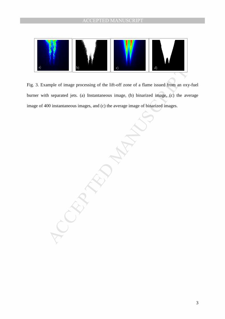
To extract the lift-off heights and the flame lengths, classical image processing (binarization,
average, rms, thresholding) was used on all the images for each configuration. To determine
the lift-off position of flame, it is necessary to perform a binarization then a detection of
contour. The choice of threshold of binarization is delicate since we have to eliminate the
noise from the images without affecting the signal. The method used here consists in locating
the region of interest where the flame is stabilized and then to make a profile of the signal
along the axis of object. Threshold value is taken at the inflection point of the intensity
profile. Lift-off height is determined as the closest point to the burner where the signal
appears. Fig. 3 shows an example of image processing for OH chemiluminescence in the
stabilization region.

6
The flame length estimation is based on the visualization at the flame top. Fig. 4a shows an
example of instantaneous images of the flame top. After binarization, the flame length can be
measured for each configuration as shown in Fig. 4b. To do so, the pixel corresponding to the
end of flame (highest position) is extracted and the average of these maximum values on all
acquired images is calculated, following the expression:
n
ZZL
ni
1ii
0f
∑=
=+= (2)
where Z0 is the exit burner – base flame distance, Zi is the height of the flame in the image i
and n is the number of instantaneous images used for the processing (Fig. 4b).
The experimental results related to the flame characteristics for several configurations of
burner are summarized in Table 2. The lift-off positions (vertical position, Zlo and horizontal
position, Xlo) and the flame lengths Lf are given as a function of nozzle diameters (ngd and
oxd ) and the separation distance between the jets (S). The horizontal position of flame lift-off
(or radius) has a zero value at the centre of the central jet of the natural gas.

7
3. Modelling technique
Neural computation requires several steps to allow the predictions of the correlations between
the input and output of the present problem. The basic mechanism behind ANN is the neuron
activity. The neuron is a mathematical processing unit that receives an input (a number),
transforms it (by simple mathematical operations) and forward it to other neurons.
Details about the methodology can be found in [13,20]. In the following, we will stick to a
concise description of the technique.
Step1: definition of the input/output sets
Three burner parameters (the internal diametersngd , oxd and the separation distance between
the jets S) are attributed each one neuron. This set of neurons represents the input pattern. The
output pattern represents the flame characteristics (the vertical and horizontal lift-off positions
Zlo, Xlo and the flame lengths Lf ). All variables are expressed in a dimensionless form.
Indeed, since the parameter range can influence the quality of the predictions, all variables are
expressed in the range 0-1, using the upper and lower limits available for each variable. Such
pre-processing assumes the following conversion scheme, which is detailed in previous
studies
i mini
max min
x xy
x x
−=−
(3)
where yi is the dimensionless form of the variable xi. xmin and xmax represent the window range
of variable xi. These limits are summarized in Table 3 for all studied parameters.
Each neuron is connected the other neurons following a feed-forward scheme. This writes
i ij jI W O= (4)
where Ii is the input of neuron i belonging to the forward layer, Oj is the output of a given
neuron j from the backward layer Wij is the weight parameter that relates neurons i and j.
A typical sketch of the neuron connectivity can be found in [13]

8
The output of a given neuron is related to its input using the expression [21]
( )ii
1O
1 exp I=
+ −
where the sigmoid function is used to nonlinearly transform the input of each neuron in the
network structure. The output is thus bounded between 0 and +1.
Step2: building the database
As the number of experimental sets is limited (29 experiments as shown in Table 2), small
ANN structures are used. A typical structure comprises the input and output patterns plus
hidden units (neurons) organised in intermediate layers. The more units in the hidden layers,
the more experimental sets needed for the optimisation of the ANN structure. Thus, it is
decided to keep one intermediate layer for which the number of neurons is varied between 1
and 6. Following the correlation between weight population and database size, we are slightly
below the lower bound when 6 neurons are used in the hidden layer (see for example [13]).
We vary the neuron number between the abovementioned bounds to demonstrate where the
robustness of neural network is applicable. We know that a unique neuron in the hidden layer
is insufficient to give reliable prediction and we know also that 6 neurons is larger than the
weight population. Thus, optimal neural network have to be searched between these bounds.
The database is organised in two main categories: training and test categories. The training set
data are picked out randomly and varied between 0% to 100%, where the percentage is
expressed with respect to the whole database.
Step3: performing the analysis
Training category is used to tune the neuron connections, i.e., weights [20]. In the test
procedure, experimental sets are used without correcting any weight. The convergence of the
procedure is obtained if the error evolution of the training and test steps stabilise. The
procedure is robust if these quantities are close to each other and small enough. The error is
obtained by comparing the experimental and numerical response for a given input condition.

9
Two main convergence criteria are studied: the average and maximum errors calculated with
respect to the submitted cases. The average quantity is expressed as a mean square error.
Step4: solving the problem of equivalent ANN structures
The ANN structures (obtained by varying the neuron number) are classified based on the
smallest training and testing errors and also on the basis of the lowest percentage of the data
in the training set used for the optimisation.

10
4. Results and discussion
Fig. 5 shows a typical optimisation procedure of the ANN structure. The convergence criteria
are two average and two maximum errors. The evolution of training errors as function of
iteration level up to 1000 itrs well depicts the stabilisation of the convergence criteria beyond
300 cycles (Fig. 5a). We have selected a small iteration number compared to what is reported
in the literature because we have used an efficient training algorithm that can lead to
significant overtraining. The final iteration number is large enough to obtain a steady state
asymptotic error evolution (significant changes are within the first 300 iterations). The
maximum iteration number is lower than 10 000 to avoid overtraining. Fig. 5a well shows that
overtraining is not attained since the maximum error is higher than the average error. When
increasing the number of neurons from 1 to 6, the final training error decreases. Such a
decrease is explained by the increase of the weight number (increase of connections between
neurons). This has the consequence to give more variables to the system to find the best
weight configuration with respect to a given set of submitted samples. However, when the
weight number is too large, the prediction beyond the operating window becomes less evident
to trust because a proper prediction requires more experimental sets. In our case, we do not
need to have a large neuron number as suggested in Fig. 5a because even in the worst case
(one unique neuron in the hidden layer), the maximum error is still less than 5%. Fig. 5b
shows the evolution of the test criterion for a training database size of 70%. Convergence of
the criterion is obtained irrespective of the neuron number. In particular, with two neurons in
the hidden layer, the test errors are the smallest ones. The difference between the maximum
and the average error seems more significant compared to the training procedure.
Fig. 6 shows the training and test error maps after an optimisation procedure performed on the
output Zlo. Note that these maps correspond to the error values at the final iteration level

11
where convergence is assumed. Both criteria training and test errors exhibit steady state
evolution whatever is the difference between the criteria. The error domain is two-
dimensional with the horizontal axis representing the number of neurons (NN) and the vertical
one being the percentage of training samples (Tr). Robustness of the neural network can be
thus determined. A robust net structure corresponds to a smallest difference between training
and test errors combined to the smallest training set and larges test set. The average training
error varies between 0.003 and 0.017 in the case of the training procedure (Figure 6a). The
error domain is nearly homogeneous. It shows that the training error is significantly
dependent on the percentage of training samples rather than on the number of neurons. This
result can be inferred to the fact that the large number of iterations (1000 in the present case)
is sufficient to enforce the convergence whatever is the neuron number. It seems that at
Tr=50%, the error decreases with the decrease of neuron number. Two optimal configurations
are found corresponding to (NN=2, Tr=70%) and (NN=6, Tr=50%).
In the case of test procedure, the predicted map contains discriminating information (Fig. 6b)
as we can see clearly that the decrease of training samples (i.e., the decrease of test database
size) predicts the minimum error. The influence of the neuron number is minor. Thus, it
makes sense to choose the configuration (NN=2, Tr=70%) as being the optimal condition.
Our selection is based on the fact with 2 neurons the weight population is reduced so that the
predictions are more reliable. This situation is comparable to searching optimal function with
few parameters to fit the experimental data. Of course, selecting the optimal neural structure
based on a smaller training set would be also reasonable.
Fig. 7 compares the experimental and predicted responses at the final iteration level in the
case of Zlo and for two particular ANN structures. Both responses are expressed in reduced
units. For both cases, the slope of the curve is close to unity with a satisfying correlation
factor (R²>0.96). Since training and test data are different, we are certain that the causal

12
correlations encoded in the ANN structure are well captured. Again, the slight deviation of the
numerical results with regard to the experimental values attests that overtraining is not
attained.
The result of the optimisation procedure described above is still valid for the two other
outputs. In the following, the exploitation of the ANN predictions is detailed. This
exploitation considers the optimal ANN structure for which the weight parameters are fixed.
It considers also different combinations of input parameters varied in a continuous way and
for which the outputs are calculated for each input combination.
Fig. 8a shows the effect of varying separation distance and the oxygen jet diameter on the
value of lift-off height of flame for a given value of ngd . Zlo is found to be the highest one for
a large S and a small oxd values. The tendency seems to be polynomial rather than linear. The
increase of S delays the mixing of reactants and consequently the combustion starts later at
larger distances from burner. This obvious result is well reported in the literature [11-12]. The
decrease of oxd leads to the increase of the oxygen jet velocity because a fixed flow rate is
used. Thus, the flame base is moved far away from the nozzles exits [11, 22-25]. Fig. 8b
shows the same evolution map for a larger ngd value. Despite the similar tendency obtained
using the combination of S and oxd (i.e., the increase of Zlo is correlated to the increase of
S/ oxd ), a smaller domain where this effect prevails is noticed. Indeed, as illustrated in Fig. 8b,
the region below the solid line exhibits the smallest Zlo values. In fact, a small natural gas jet
diameter increases the jet velocity because of the constant flow rate. Thus, when increasing
ngd , smaller Zlo values are expected for a given combination of S and oxd .
Fig. 8c depicts the effect of S and ngd on Zlo for a given value of oxd . It is clearly shown here
that a polynomial evolution is predicted in this case. Zlo is found to increase with the increase
of the ratio S/ ngd . It can be demonstrated (all results are not shown here) that any of the

13
combinations (S, oxd ), (S, ngd ) or ( oxd , ngd ) leads firmly to a polynomial correlation where
Zlo increases with the increase of S/oxd , S/ ngd or 1/( ngd x oxd ).
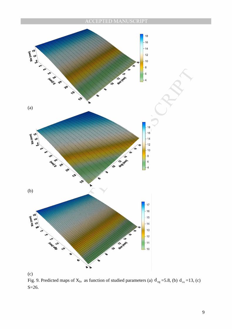
The effect of the burner parameters on horizontal position of flame base is shown in Fig. 9.
When combining S and oxd for a fixed value of ngd , it is predicted that Xlo increases non-
linearly only with the increase of S for any particular value of oxd (Fig. 9a). In fact, the
horizontal position of the stabilisation point is fully dependent on the spacing between the jets
due to geometrical considerations [4]. When increasing ngd , no major change in Xlo is
observed either in magnitude nor in trend, which means that the unique control parameter is
the spacing between the jets.
The combined effect of separation distance between the jets and the natural gas jet diameter
on horizontal position of the stabilisation point is shown in Fig. 9b. The trend is different from
the first case. Despite that S is the first control parameter (Xlo increases when S increases),
ngd plays a secondary role as predicted in Fig. 9b (slightly higher levels of Xlo are predicted
when increasing ngd ). In Fig. 9c is presented the evolution of Xlo as function of ngd and oxd .
Again, the effect of ngd is predominant compared to oxd . The higher is ngd value, the larger
is Xlo response. This last trend confirms the previous results (Figs. 9a, 9b) in the sense that a
classification of the influential effects can be deduced based on the analysis of all maps shown
in Fig. 9. In fact, S is the major control factor, ngd is the intermediate one and oxd has the
smallest effect. The interaction effects are more subtle except when combining S and ngd .
The analysis of the third output (the flame length) as function of studied parameters reveals
the following ideas summarized in Fig. 10. When combining S and oxd (Fig. 10a), it is
predicted that the evolution of Lf is positively correlated to the evolution of the product S x
oxd . This actually represents the unique combination of burner parameters where an
14
interaction effect is highlighted. Indeed, when comparing this result to that corresponding for
example to the combination (S, ngd ), it is found that only S has an effect on Lf (Fig. 10b).
This is also confirmed by the last trend (Fig. 10c) where the increase of Lf is only attributed to
the increase of oxd . The prevailing effect of S can be deduced from the mixing process of
natural gas and oxygen for which the increase of S means a delay of the combustion start and
an increase of the flame length [3].
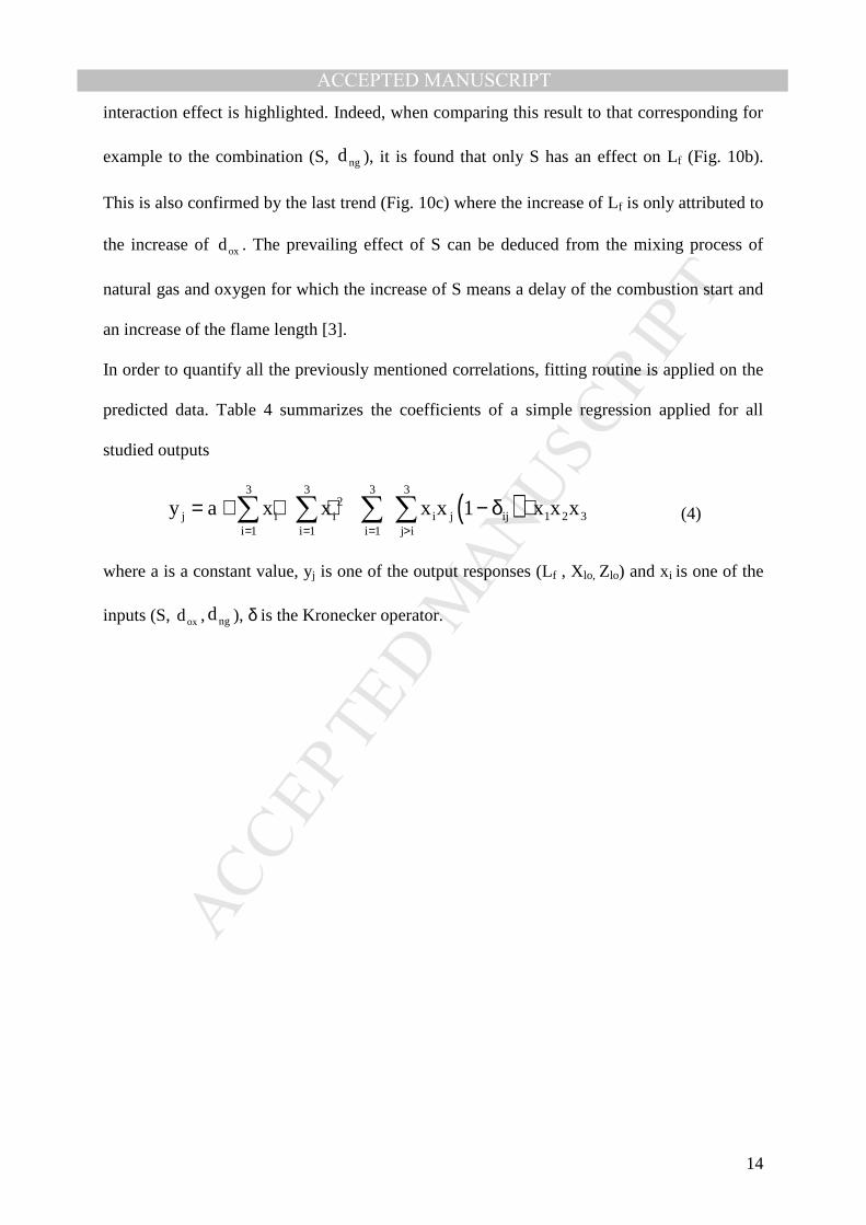
In order to quantify all the previously mentioned correlations, fitting routine is applied on the
predicted data. Table 4 summarizes the coefficients of a simple regression applied for all
studied outputs
( )3 3 3 3
2j i i i j ij 1 2 3
i 1 i 1 i 1 j i
y a x x x x 1 x x x= = = >
= + + + − δ +∑ ∑ ∑ ∑ (4)
where a is a constant value, yj is one of the output responses (Lf , Xlo, Zlo) and xi is one of the
inputs (S, oxd , ngd ), δ is the Kronecker operator.

15
5. Conclusions
The combined effect of burner parameters (S: separation distance between the jets, oxd and
ngd : the jet diameters of oxygen and natural gas, respectively) on the studied flame
characteristics suggests the following correlations:
• Lift-off height of flame is dependent on all burner parameter interactions in the sense
that larger heights are proportional to single terms: -8(ngd + oxd +0.03S), quadratic
terms 0.03( ngd ² + oxd ²+0.5S²), simple interactions 0.5(ngd x oxd +0.3S( ngd x oxd )) and
all terms interaction –0.016(oxd S ngd ).
• The horizontal position of the flame lift-off is dependent on a unique burner parameter
interaction 0.01(S ngd ). If we exclude the former interaction term, a simple linear
correlation (R²=0.92) is sufficient to represent truly the correlations. This correlation
highlights the prevailing role of S and ngd compared to oxd : Xlo∝ 0.3(S+ ngd -
0.06 oxd ).
• The flame length is predicted to depend positively on all parameters. Combining S and
oxd allows better results (in this case, the interaction term is 0.64). S and oxd represent
here the most influential parameters to vary Lf.

16
References
[1] A. Ivernel, P. Vernotte, Revue Générale de Thermique 210 (1979) 375-391.
[2] C.E. Baukal, B. Gebhart, Int. J. Heat Mass Tran. 40(11) (1997) 2539-2547.
[3] J.C. Sautet, T. Boushaki, L. Salentey, B. Labegorre, Combustion Sci. Technol. 178 (2006)
2075-2096.
[4] T. Boushaki, J-C. Sautet, L. Salentey, B. Labegorre, Int. Communication Heat Mass
Transfer 34 (2007) 8-18.
[5] T. Boushaki, J-C. Sautet, Exp Fluids 48 (2010) 1095–1108.
[6] A. Krothapalli, D. Bagadanoff, K. Karamchetti, AIAA journal 18 (8) (1980) 945-950.
[7] S. Raghunatan, I.M. Reid, AIAA journal 19 (1980) 124-127.
[8] I. Yimer, H.A. Becker, E.W. Grandmaison, A.I.C.H.E Journal 74 (1996) 840-851.
[9] A. K. Moawad, N. Rajaratnam, S.J. Stanley, J. hydraulic research 39 (2) (2001) 163-168.
[10] A.O.P. Leite, M.A. Ferreira, J.A. Carvalho, Int. Comm. Heat Mass Transfer 23 (7)
(1996) 959-970.
[11] R. Menon, S.R. Gollahali, Combust. Sci. Technol. 60 (1998) 375-389.
[12] B.J. Lee, J.S. Kim, S. Lee, Combustion Sci. Technol. 176 (2004) 481-497.
[13] S. Guessasma, G. Montavon and C. Coddet, Comput. Mat. Sci. 29 (3) (2004), 315-333.
[14] H. Deng, S. Guessasma, D. Benkrid, G. Montavon, H. Liao, S. Abouddi, C. Coddet,
Numerical Heat Transfer, Part A 47 (6) (2005) 593-607.
[15] H. Fall, S. Guessasma, W. Sharon, Engineering Structures, 28 (2006) 1787-1794.
[16] B . Lenze, ME. Milano, R . Günther, Combust Sci Tech 11 (1975) 1–8.
[17] C.E. Baukal, Industrial Burners Handbook, CRC Press, 2003.
[18] M. DiTaranto, J.C. Sautet, J.M. Samaniego, Experiments in Fluids, 30 (2001) 253-261.
[19] D.S. Dandy, S.R.Vosen, Combustion Science and Technology, 82 (1992) 131-150.

17
[20] S. Guessasma, Z. Salhi, G. Montavon, P. Gougeon and C. Coddet, Mat. Sci. Eng. B
110 (3) (2004) 285-295.
[21] T. Sahraoui, S. Guessasma, N Fenineche, G. Montavon, C. Coddet, Mat. Letters, 58(5)
(2004) 654-660.
[22] G.T. Kalghatgi, Combustion Sci. Technol. 41 (1984) 17–29.
[23] L. Muniz, M.G. Mungal, Combustion and Flame 111 (1997) 16-31.
[24] R.W. Schefer, M. Namazian, J. Kelly, Proc. Int. 22th Symposium on Combustion/The
Combustion Institute, Seattle, USA, (1988) 833-842.
[25] A. Cessou, C. Maurey and D. Stepowski, Combustion and Flame 137 (4) (2004) 458-
477.

18
Figure captions
Fig. 1. Schematic diagram of separated-jet burner. Fig. 2. Schematic diagram of the Chemiluminescence setup. Fig. 3. Example of image processing of the lift-off zone of a flame issued from an oxy-fuel
burner with separated jets. (a) Instantaneous image, (b) binarized image, (c) the average
image of 400 instantaneous images, and (c) the average image of binarized images.
Fig. 4. (a) Examples of OH instantaneous images at the flame top and (b) their corresponding
binarized image.
Fig. 5. Evolution of the average and maximum convergence criteria as function of iteration
level for an increasing number of neurons in the hidden layer. Runs are performed in the case
of Zlo output – training database 70%.
Fig. 6. (a) training and (b) test error maps relative to the output Zlo as function of neuron
number and ratio from the whole database of samples used for training.
Fig. 7. Comparing experimental and predicted Zlo for two neural nets (optimal condition
NN=1, TR=50% and none-optimized condition NN=6, TR=100%).
Fig. 8. Predicted maps of Zlo as function of studied parameters. (a) ngd =4, (b) ngd =11, (c)
oxd = 15.
Fig. 9. Predicted maps of Xlo as function of studied parameters (a) ngd =5.8, (b) oxd =13 (c)
S=26.
Fig. 10. Predicted maps of Lf as function of studied parameters. (a) ngd =5.8, (b) oxd =8 (c)
S=17.

19
List of Tables
Table 1. Operating conditions of the burner parameters.
Table 2. Experimental database used to assess lift-off positions of flame (Zlo and Xlo) and
flame length (Lf) as a function of nozzles diameters (for the natural-gas jet, ngd and the
oxygen jet, oxd ) and the separation distance between the jets (S).
Table 3. Window range of the studied parameters.
Table 4. Regression coefficients based on ANN predicted results and using different
approximations.

1
Table 1. Operating conditions of the burner parameters.
Central natural gas jet One lateral oxygen jet
dng (mm) 0
ngU (m/s) Reng dox (mm) 0
oxU (m/s) Reox
4 53.3 16152
6 25.4 10792
8 14.3 8101
10 9.1 6444
6 23.6 10727
6 25.4 10792
8 14.3 8101
10 9.1 6444
8 13.4 8121 6 25.4 10792
8 14.3 8101
Table(s)

2
Table 2. Experimental database used to assess lift-off positions of flame (Zlo and Xlo) and
flame length (Lf) as a function of nozzles diameters (for the natural-gas jet, ngd and the
oxygen jet, oxd ) and the separation distance between the jets (S).
Exp. # Inputs Outputs
ngd (mm) oxd (mm) S (mm) Zlo (mm) Xlo (mm) Lf (mm)
1 4 6 7 56.14 3.31 463
2 4 8 8 14.43 3.19 527
3 4 8 12 44.27 4.91 568
4 4 8 16 77.90 6.31 -
5 4 10 9 10.54 3.26 -
6 4 10 12 27.30 4.53 -
7 4 10 16 39.96 5.83 -
8 6 6 8 19.03 3.94 461
9 6 6 12 46.08 6.55 520
10 6 6 16 61.78 8.52 548
11 6 6 20 74.71 10.47 593
12 6 6 30 92.08 13.90
13 6 8 9 11.84 4.17 564
14 6 8 12 23.77 5.54 580
15 6 8 16 38.39 7.36 611
16 6 8 20 49.12 9.14 656
17 6 8 30 75.16 12.38 -
18 6 10 10 - - -
19 6 10 12 18.35 5.41 -
20 6 10 16 28.64 6.80 -
21 6 10 20 43.34 8.53 -
22 8 6 9 11.69 4.93 452
23 8 6 12 16.62 6.64 517
24 8 6 16 33.19 8.65 507
25 8 6 20 47.48 11.19 592
26 8 8 10 - - 568
27 8 8 12 17.48 6.00 582
28 8 8 16 28.82 7.95 608
29 8 8 20 45.92 9.90 672

3
Table 3. Window range of the studied parameters.
Limit Inputs Outputs
ngd (mm) oxd (mm) S (mm) Zlo (mm) Xlo (mm) Lf (mm)
xMin 4 4 7 0 0 0
xmax 20 20 50 - - -

4
Table 4. Regression coefficients based on ANN predicted results and using different
approximations.
a oxd ngd S oxd ² ngd ² S ² ngd x oxd oxd xS ngd xS ngd x oxd xS R²
Zlo
109 -8.1 -8.3 -0.26 0.029 0.033 0.014 0.515 0.143 0.138 -0.016 0.92
43 -2.6 -2.8 2.0 0.03 0.03 0.01 0.06 -0.05 -0.05 0.89
69 -3.3 -3.6 0.82 0.03 0.03 0.01 0.86
53 -2.6 -2.8 1.6 0.85
Xlo
-4.4 -0.13 0.67 0.68 0.0010 -0.0031 -0.0048 0.0040 0.0022 -0.0092 -0.0001 0.99
-4.7 -0.11 0.69 0.69 0.0010 -0.0030 -0.0048 0.0017 0.0012 -0.0102 0.99
-2.1 -0.04 0.44 0.59 0.0004 -0.0036 -0.0048 0.97
1.3 -0.03 0.35 0.31 0.94
Lf
-76 76 0.85 18 -1.2 -0.0004 -0.0586 -0.0002 -0.6230 0.0099 -0.0016 0.99
-82 77 1.40 18 -1.22 -0.0004 -0.059 -0.05 -0.64 -0.0094 0.99
147 58 0.58 11 -1.22 -0.0004 -0.06 0.93
328 29 0.58 7 0.90

1
Fig. 1. Schematic diagram of separated-jet burner.
S
dox dng dox
Oxygen Natural gas Oxygen x
y z
S
Figure(s)

2
Fig. 2. Schematic diagram of the Chemiluminescence setup.
CCD Control Unit
Furnace
PC of data
acquisition
ICCD camera UG 11 filter
UV lens
Burner
3
Fig. 3. Example of image processing of the lift-off zone of a flame issued from an oxy-fuel
burner with separated jets. (a) Instantaneous image, (b) binarized image, (c) the average
image of 400 instantaneous images, and (c) the average image of binarized images.
a)
b)
c)
d)

4
(a)
(b)
Fig. 4. (a) Examples of OH instantaneous images at the flame top and (b) their corresponding
binarized image.
Zi
Lf = Z0+Zi/n

5
0 200 400 600 800 1000
0.01
0.02
0.03
0.04
0.05
0.06
0.07
0.08
AVERAGE
1
2
4
6
Tra
inin
g e
rro
r (-
)
iteration level (-)
zl0:
MAXIMUM
1
2
4
6
(a)
0 200 400 600 800 1000
0.01
0.02
0.03
0.04
0.05
0.06
0.07
0.08
AVERAGE: 1, 2, 4, 6
test e
rro
r (-
)
iteration level (-)
zl0:
MAXIMUM: 1, 2, 4, 6
(b)
Fig. 5. Evolution of the average and maximum convergence criteria as function of iteration
level for an increasing number of neurons in the hidden layer. Runs are performed in the case
of Zlo output – training database 70%.

6
NN (-)
Tr (%)
AveTrn
(%)
(a)
NN (-)
Tr (%)
AveTst
(%)
(b)
Fig. 6. (a) training and (b) test error maps relative to the output Zlo as function of neuron
number and ratio from the whole database of samples used for training.

7
0.00 0.02 0.04 0.06 0.08 0.10 0.12 0.14 0.16 0.18 0.20 0.22 0.24 0.26
0.00
0.02
0.04
0.06
0.08
0.10
0.12
0.14
0.16
0.18
0.20
0.22
0.24
0.26
0.28
TR=100%,NN=6
TRAIN (EXP=1.0116PRED-0.0015 (R²=0.987)
EX
P (
-)
PRED(-)
TR=50%,NN=1
TRAIN (EXP=1.0083PRED-0.001 (R²=0.985)
TEST (EXP=1.0874PRED-0.014 (R²=0.960)
Fig. 7. Comparing experimental and predicted Zlo for two neural nets (optimal condition
NN=1, TR=50% and none-optimised condition NN=6, TR=100%).

8
(a)
(b)
(c)
Fig. 8. Predicted maps of Zlo as function of studied parameters. (a) ngd =4, (b) ngd =11, (c)
oxd = 15.
9
(a)
(b)
(c)
Fig. 9. Predicted maps of Xlo as function of studied parameters (a) ngd =5.8, (b) oxd =13, (c)
S=26.

10
(a)
(b)
(c)
Fig. 10. Predicted maps of Lf as function of studied parameters. (a) ngd =5.8, (b) oxd =8, (c)
S=17.

1
Fig. 1. Schematic diagram of separated-jet burner.
S
dox dng dox
Oxygen Natural gas Oxygen x
y z
S

2
Fig. 2. Schematic diagram of the Chemiluminescence setup.
CCD Control Unit
Furnace
PC of data acquisition
ICCD camera UG 11 filter
• •
UV lens
Burner

3
Fig. 3. Example of image processing of the lift-off zone of a flame issued from an oxy-fuel
burner with separated jets. (a) Instantaneous image, (b) binarized image, (c) the average
image of 400 instantaneous images, and (c) the average image of binarized images.
a)
b)
c)
d)

4
(a)
(b)
Fig. 4. (a) Examples of OH instantaneous images at the flame top and (b) their corresponding
binarized image.
Zi
Lf = Z0+ΣZi/n

5
0 200 400 600 800 1000
0.01
0.02
0.03
0.04
0.05
0.06
0.07
0.08
AVERAGE 1 2 4 6
Tra
inin
g er
ror
(-)
iteration level (-)
zl0:
MAXIMUM 1 2 4 6
(a)
0 200 400 600 800 1000
0.01
0.02
0.03
0.04
0.05
0.06
0.07
0.08
AVERAGE: 1, 2, 4, 6
test
err
or (
-)
iteration level (-)
zl0:
MAXIMUM: 1, 2, 4, 6
(b)
Fig. 5. Evolution of the average and maximum convergence criteria as function of iteration
level for an increasing number of neurons in the hidden layer. Runs are performed in the case
of Zlo output – training database 70%.

6
NN (-)
Tr (%)
AveTrn (%)
(a)
NN (-)
Tr (%)
AveTst (%)
(b) Fig. 6. (a) training and (b) test error maps relative to the output Zlo as function of neuron
number and ratio from the whole database of samples used for training.

7
0.00 0.02 0.04 0.06 0.08 0.10 0.12 0.14 0.16 0.18 0.20 0.22 0.24 0.26
0.00
0.02
0.04
0.06
0.08
0.10
0.12
0.14
0.16
0.18
0.20
0.22
0.24
0.26
0.28
TR=100%,NN=6 TRAIN (EXP=1.0116PRED-0.0015 (R²=0.987)
EX
P (
-)
PRED(-)
TR=50%,NN=1 TRAIN (EXP=1.0083PRED-0.001 (R²=0.985) TEST (EXP=1.0874PRED-0.014 (R²=0.960)
Fig. 7. Comparing experimental and predicted Zlo for two neural nets (optimal condition
NN=1, TR=50% and none-optimised condition NN=6, TR=100%).

8
(a)
(b)
(c) Fig. 8. Predicted maps of Zlo as function of studied parameters. (a) ngd =4, (b) ngd =11, (c)
oxd = 15.

9
(a)
(b)
(c) Fig. 9. Predicted maps of Xlo as function of studied parameters (a) ngd =5.8, (b) oxd =13, (c)
S=26.

10
(a)
(b)
(c) Fig. 10. Predicted maps of Lf as function of studied parameters. (a) ngd =5.8, (b) oxd =8, (c)
S=17.


