
Preservation technology investment, trade credit and partial backordering model for a
non-instantaneous deteriorating inventory
Abu Hashan Md Mashud1, Hui-Ming Wee2* and Chiao-Ven Huang2
1Department of Mathematics, Hajee Mohammad Danesh Science and Technology University,
Dinajpur-5200, Bangladesh 2Department of Industrial and Systems Engineering, Chung Yuan Christian University, 200
Chung-Pei Rd., 32023, Chung-li, Taiwan
[email protected]; [email protected]; [email protected]
Abstract
In a perfectly transparent and competitive market, suppliers must provide a competitive pricing
and service for their customers. The aim of this study is to provide an insight into how
preservation technology and credit financing could be used both to reduce the deterioration rate
as well as to provide flexible financing for retailers. The methodology is to optimize the cycle
length, selling price, the amount of preservation technology and credit financing using inventory
theory. The result derived is an optimal total profit per unit time for the system. Finally, using
MATLAB 2017a, it is shown graphically that the profit function is concave. The sensitivity
analysis is illustrated using Lingo 17. The study not only provides insights to business managers
in making wise managerial decisions, it also enables them to weigh the pro and con of
implementing preservation technology and credit financing.
Keyword: non-instantaneous deterioration; price dependent demand; partial backlogging;
preservation technology; trade credit.
1. Introduction
Inventory is defined as idle stocks in a supply chain. The management of inventory is critical
factor in the day-to-day operation of an enterprise, therefore a proper system to manage
inventory is critical. One of the key factors to consider in inventory modeling is deterioration.
Deterioration is the evaporation, decay or damage of inventory. Inventory has been the focus of
This provisional PDF is the accepted version. The article should be cited as: RAIRO: RO, doi: 10.1051/ro/2019095

many researches for over a century. Mishra (2013) projected an inventory model for controllable
deterioration with time-varying demand and time-varying holding cost. Mishra (2014) presented
an inventory model with controllable deterioration rate and time-dependent demand. Pandey et
al. (2017) established an inventory model with negative exponential demand and probabilistic
deterioration under backlogging. Nobil et al. (2019) developed a model for single machine lot
scheduling problem for negative exponential deteriorating items. Nobil et al. (2019) projected a
model for economic lot size problem for cleaner manufacturing system with another interesting
parameter warm-up period. A two-warehouse model with increasing demand under time-varying
deterioration is developed by Sett et al. (2012). Sarkar & Sarkar (2013) developed an inventory
model with partial backlogging and stock dependent demand. Palanivel et al. (2016) presented an
inventory model for imperfect items with stock dependent demand under permissible delay in
payments. Shaikh et al. (2017) presented a model considering stock and price sensitive demand
under fully backlogged shortages. Mashud et al. (2018) developed an inventory model for non-
instantaneous inventory model with same demand. Nobil et al. (2018) developed an economic
production quantity model with and without shortages for imperfect products. Dey et al. (2019)
projected an inventory model considering price dependent demand with setup cost reduction.
In terms of preservation of products, Dye and Hseigh (2012) developed an inventory model
considering the investment in preservation technology. Dye (2013) also developed a non-
instantaneous deteriorating inventory model with preservation technology. Singh (2016)
developed an EOQ model for stock-dependent demand deteriorating items with preservation
technology; while Yang et al. (2015) introduced optimal dynamic trade credit and preservation in
their model.
Goyal (1985) was one of the first researchers who developed an EOQ model under
permissible delays in payments. Aggarwal and Jaggi (1995) introduced an ordering policy for
deteriorating items under permissible delays in payments. Tsao et al. (2008) considered
deteriorating items inventory model with price and time-dependent demand under permissible
delays in payments. Pal (2018) developed a production inventory model for imperfect products
with permissible delay in payments under shortages. Yang et al. (2015) considered the
preservation technology investment to control the deterioration for a time-dependent demand rate
under trade credit policy. Teng et al. (2012) developed an EOQ model with trade credit financing

for non-decreasing demand. Chen et al. (2015) modified this model by introducing upstream and
downstream trade credit policy in his time-varying deteriorating model with cash flow. Lastly,
Tiwari et al. (2016, 2017) developed a non-instantaneous deteriorating inventory model
considering inflation and trade credit policy in a two-warehouse environment. A comparison of
the present study with the previous researches is shown in Table 1.
Table 1. A comparison of the present study with the previous researches
Authors Demand pattern Deterioration Preservation
technology Shortages Trade credit
Dye and Hsieh (2012) Constant Time-dependent Yes Partial
Backordering No
Hsieh and Dye (2013)
Time-dependent Constant Yes No No
He and Huang (2013)
Price-dependent Constant Yes No No
Dye (2013) Constant Non-instantaneous Yes Partial backordering No
Zhang et al. (2014)
Price dependent Constant Yes No No
Liu et al. (2015) Price dependent Constant Yes No No
Lu et al. (2016) Price and stock dependent Constant No No No
Jaggi et al. (2017) Price-dependent Non-instantaneous No Complete
backordering Yes
Li et al (2018) Price-dependent Non-instantaneous Yes No No
Tiwari et al. (2018) Price-dependent Non-instantaneous No Partial
backordering Yes
Mishra et al. (2018) Price-dependent Constant Yes No Yes
This paper Price dependent Non-instantaneous Yes Partial
backordering Yes
The objective of this paper is to optimize the cycle length, selling price considering preservation
technology. Three numerical examples were used to illustrate the theory. Graphical
representations are used to illustrate the results.
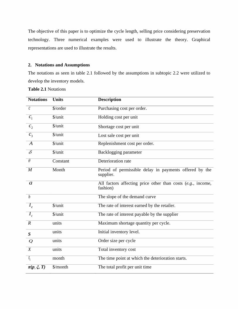
2. Notations and Assumptions
The notations as seen in table 2.1 followed by the assumptions in subtopic 2.2 were utilized to
develop the inventory models.
Table 2.1 Notations
Notations Units Description
c $/order Purchasing cost per order.
1c $/unit Holding cost per unit
2c $/unit Shortage cost per unit
3c $/unit Lost sale cost per unit
A $/unit Replenishment cost per order.
δ $/unit Backlogging parameter
Constant Deterioration rate
M Month Period of permissible delay in payments offered by the supplier.
a All factors affecting price other than costs (e.g., income, fashion)
b The slope of the demand curve
eI $/unit The rate of interest earned by the retailer.
cI $/unit The rate of interest payable by the supplier
R units Maximum shortage quantity per cycle.
S units Initial inventory level.
Q units Order size per cycle
X units Total inventory cost
1t month The time point at which the deterioration starts.
π(p, ξ, T) $/month The total profit per unit time
θ

Dependent Variable
2t month The time point at which the shortages are allowed.
Decision variables
p month Unit selling price
T month The total length of the inventory cycle.
ξ $/unit Preservation technology cost
2.2 Assumptions
1. The model considered a linear price-dependent demand pattern ( )D p a bp= − (i.e.
demand function depends on price for a single deteriorating item).
2. The considered deterioration rate is constant and depends on the stock
amount.
3. No replacement or repairs on deteriorating products were considered for the whole
period.
4. Lead-time is negligible and the replenishment rate is infinite.
5. The total planning horizon considered in the inventory system is infinite.
6. The relationship between the deterioration rate and the preservation technology
investment parameter always satisfies the conditions ( ) ( )2
20 , 0.m mξ ξξ ξ
∂ ∂< >
∂ ∂The
research considered that ( ) 1am e ξξ −= ; where ( )m ξ is the deterioration rate with the
investment of preservation technology,θ is the deterioration rate without the preservation
technology investment, and 1a is the sensitive parameter of investment to the
deterioration rate which is similar as Mishra et al. (2018) and He and Huang (2013).
7. The backlogging rate during the stock out period is considered as a variable dependent on
the length of waiting time for the next replenishment. Therefore, the backlogging rate for
negative inventory is given by( )1
1 T tδ+ −, where δ is a backlogging parameter, and
( )T t− is the waiting time.
)10( <<< θθ

3. Mathematical formulations
Figure 1 shows the graphical demonstration of inventory versus time wherein the inventory level
at any time interval between 0 t T≤ ≤ is represented by ( )I t . It is important to present that the
level of inventory ( )I t was portrayed due to demand in the period [ ]10, t and it dropped to zero at
2t t= owing to the deterioration and demand in the period [ ]1 2,t t . Afterwards, shortages were
permitted to take place and the total demand in the period [ ]2 ,t T is partially backordered.
Figure 1. Graphical presentation of inventory vs. time
The following differential equations illustrate the inventory model:
Change in inventory level,
( ) ( )1dI ta bp
dt= − − 10 t t< ≤ (1)
With the initial and boundary conditions as at 0t = .
The solution for Eq. (1) is as follows:
( ) ( )1I t S a bp t= − − , 10 t t< ≤ (2)
and
StI =)(1
T t1 t2
Time
Inventory

( ) ( ) ( ) ( )22 1 2
dI tm I t a bp t t t
dtθ ξ+ = − − < ≤
(3)
with the boundary condition ( )2 0I t = at 2t t= , the solution for Eq. (3) is as follows:
( ) ( )( )
( )( )( )22 1m t ta bp
I t em
θ ξ
θ ξ−−
= − 1 2t t t< ≤ (4)
where ( )I t is continuous at 1t t= , hence ( ) ( )1 1 2 1I t I t= resulting in,
( ) ( )( )
( )( )2 1( )1 1m t ta bp
S a bp t em
θ ξ
θ ξ−−
= − + − .
(5)
At time, t= t2, the inventory level is zero. For t > t2, shortage occurs, the inventory level at
any time t is directed by the differential equation
( ) ( )( )
321
dI t a bpt t T
dt T tδ− −
= < ≤+ −
(6)
with the boundary condition ( )3 0I t = at 2t t= , one has:
( ) ( ) ( )( ) ( )( ){ }3 2log 1 log 1a bp
I t T t T tδ δδ−
= + − − + − 2t t T< ≤ . (7)
The maximum amount of demand, which is the backlogged is given as follows:
( ) ( ) ( )( ){ }3 2log 1a bp
R I T T tδδ−
= − = + − . (8)
Hence, the total order quantity per cycle is:
( ) ( )( )
( )( ) { }2 1( )1 2
( )1 log(1 ( ))m t t
Q S Ra bp a bpa bp t e T tm
θ ξ δθ ξ δ
−
= +
− −= − + − + + −
.
(9)
The holding cost in the entire cycle is set as
IHC = ( ) ( )1 2
1
1 1 1 20
t t
t
c I t dt c I t dt+∫ ∫
( )( )
( )( ) ( ) ( )( )2 1
21
1 1 2 122
( ) 12
m t ta bpa bp tc St e m t tm
θ ξ θ ξθ ξ
− −−
= − − − + − .
(10)
The backorder cost in the entire cycle is set as
( ) ( )( ) ( )( )
22 2
2 2 2 22
1 {log(1 ( )) log(1 ( ))}
R 1 log 1
T
tBC C D T t T t dt
D Dc T t T t T t
δ δδ
δ δδ δ
∫
= + − − + −
= + − − + − + −
. (11)
The opportunity cost due to lost sales in the entire cycle is specified in the form
( )2
311 ( )
1
T
t
LSC c a bp dtT tδ
= − − + − ∫
( ) ( ) ( )( ){ }3
2 2log 1c a bp
T t T tδ δδ−
= − − + − .
(12)
The total purchase cost per cycle is given in the form
( ) ( )( )
( )( ) { }2 1( )1 2
( )1 log(1 ( ))m t ta bp a bpPC cQ c a bp t e T tm
θ ξ δθ ξ δ
− − −= = − + − + + −
. (13)
The total sales revenue in the entire cycle is known in the form
( ) { }2 2( ) log(1 ( ))a bpSR p a bp t T tδ
δ− = − + + −
(14)
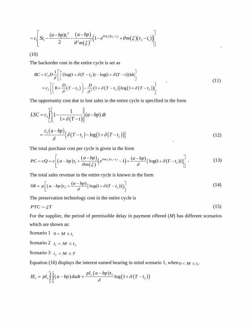
The preservation technology cost in the entire cycle is
PTC Tξ= (15)
For the supplier, the period of permissible delay in payment offered (M) has different scenarios
which are shown as:
Scenario 1 10 M t< ≤
Scenario 2 1 2t M t< ≤
Scenario 3 2t M T< ≤
Equation (16) displays the interest earned bearing in mind scenario 1, when10 M t< ≤ .
( ) ( ) ( )( )2
21 2
0 0
log 1t t
ee
pI a bp tIE pI a bp dudt T tδ
δ−
= − + + −∫ ∫

( ) ( ) ( )( )22 2
2log 12
e epI a bp t pI a bp tT tδ
δ− −
= + + − .
(16)
The interest paid to the supplier for this case is
( ) ( )1 2
1
1 1 2
t t
c cM t
IC cI I t dt cI I t dt= +∫ ∫
( ) ( ) ( ) ( )( )( )
( )( )( ) ( )( )2 1
2 21
1 2 12 12
m t tcc
t M cI a bpcI S t M a bp e m t t
mθ ξ θ ξ
θ ξ−
− − = − − − − − + − . (17)
Therefore, the total profit is
( )1 , , Xp TT
π ξ = ,
where ( )1 1X SR OC PC IHC BC LSC PTC IE IC= − − − − − − + −
( ) { }
( ) ( )( )
( )( ) { }
( )( )
( )( ) ( )( )( )
( ) ( )( ) ( )( )
2 1
2 1
2 2
( )1 2
21
1 1 2 122
2 2 2 22
3
( ) log(1 ( ))
( )1 log(1 ( ))
( ) 12
R 1 log 1
m t t
m t t
a bpp a bp t T t A
a bp a bpc a bp t e T tm
a bpa bp tc St e m t tm
D Dc T t T t T t
c a
θ ξ
θ ξ
δδ
δθ ξ δ
θ ξθ ξ
δ δδ δ
−
−
− = − + + − − − − −
− + − + + − − −−
− − − + − − + − − + − + − −
( ) ( )( )( )
( ) ( ) ( )( )
( ) ( ) ( ) ( )( )( )
( )( )( ) ( )( )2 1
22 2 2
22
2 21
1 2 12
log 12log 1
12
e e
m t tcc
T tbp pI a bp t pI a bp tT t
T t
t M cI a bpT cI S t M a bp e m t t
mθ ξ
δδ
δ δδ
ξ θ ξθ ξ
−
−− − − + + + − − + −
− − − − − − − + − + −
(18)
The corresponding optimization problem is as follows:
Problem 1. ( )1 , , Xp TT
π ξ = ,
subject to constraints 10 M t< ≤ .
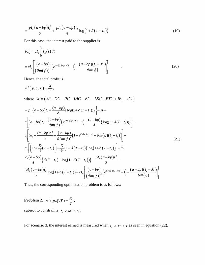
For scenario 2, the interest earned is measured when 1 2t M t< ≤ as seen in equation (19).
( ) ( ) ( )( )2
22 2
0 0
log 1t t
ee
pI a bp tIE pI a bp dudt T tδ
δ−
= − + + −∫ ∫
( ) ( ) ( )( )22 2
2log 12
e epI a bp t pI a bp tT tδ
δ− −
= + + − . (19)
For this case, the interest paid to the supplier is
( )2
2 2
t
cM
IC cI I t dt= ∫
( )( )( )
( )( )( ) ( )( )( )
2 22 1m t M
c
a bp a bp t McI e
mmθ ξ
θ ξθ ξ−
− − − = − −
. (20)
Hence, the total profit is
( )2 , , Xp TT
π ξ = ,
where ( )2 2X SR OC PC IHC BC LSC PTC IE IC= − − − − − − + −
( ) { }
( ) ( )( )
( )( ) { }
( )( )
( )( ) ( )( )( )
( ) ( )( ) ( )( )
2 1
2 1
2 2
( )1 2
21
1 1 2 122
2 2 2 22
( ) log(1 ( ))
( )1 log(1 ( ))
( ) 12
R 1 log 1
m t t
m t t
a bpp a bp t T t A
a bp a bpc a bp t e T tm
a bpa bp tc St e m t tm
D Dc T t T t T t T
c
θ ξ
θ ξ
δδ
δθ ξ δ
θ ξθ ξ
δ δ ξδ δ
−
−
− = − + + − − − − −
− + − + + − − −−
− − − + − − + − − + − + − −
( ) ( ) ( )( ){ } ( )
( ) ( )( ) ( )( )( )
( )( )( ) ( )( )( )
2
23 2
2 2
2 22 2
log 12
log 1 1
e
m t Mec
a bp pI a bp tT t T t
pI a bp t a bp a bp t MT t cI e
mmθ ξ
δ δδ
δδ θ ξθ ξ
−
− −− − + − + +
− − − − + − − − +
(21)
Thus, the corresponding optimization problem is as follows:
Problem 2. ( )2 , , Xp TT
π ξ = ,
subject to constraints 1 2t M t< ≤ .
For scenario 3, the interest earned is measured when 2t M T< ≤ as seen in equation (22).

( ) ( ) ( )( )2
23 2
0 0
log 1t t
ee
pI a bp tIE pI a bp dudt T tδ
δ−
= − + + −∫ ∫
( ) ( ) ( )( )22 2
2log 12
e epI a bp t pI a bp tT tδ
δ− −
= + + −
(22)
For this case, the interest paid to the supplier is zero.
Therefore, the total profit is
( )3 , ,T XpT
π ξ = ,
where ( )3X SR OC PC IHC BC LSC PTC IE= − − − − − − +
( ) { }
( ) ( )( )
( )( ) { }
( )( )
( )( ) ( )( )( )
( ) ( )( ) ( )( )
2 1
2 1
2 2
( )1 2
21
1 1 2 122
32 2 2 22
( ) log(1 ( ))
( )1 log(1 ( ))
( ) 12
R 1 log 1
m t t
m t t
a bpp a bp t T t A
a bp a bpc a bp t e T tm
a bpa bp tc St e m t tm
c aD Dc T t T t T t
θ ξ
θ ξ
δδ
δθ ξ δ
θ ξθ ξ
δ δδ δ
−
−
− = − + + − − − − −
− + − + + − − −−
− − − + − −
+ − − + − + − −
( ) ( )( )( )
( ) ( ) ( )( )
2
2
22 2
2
log 1
log 12
e e
T tbpT t
pI a bp t pI a bp tT T t
δ
δ δ
ξ δδ
− −−
+ − − −
− + + + −
(23)
Thus, the corresponding optimization problem is as follows
Problem 3. ( )3 , , Xp TT
π ξ = ,
subject to constraints 2t M T< ≤ .
4. Optimal Solutions and Theoretical results
The profit function considers sales revenue, ordering cost, holding cost, purchasing cost,
backordering cost, lost sale cost, preservation technology cost, interest earned, and the interest
payable. The average profit per unit time for the retailer can be expressed as:
[ ]1( , , )p T SR OC PC IHC BC LSC PTC IE IPT
π ξ = − − − − − − + − (24)

11
21 2
32
( , , ) , when 0
( , , ) ( , , ) , when
( , , ) , when
p T M tp T p T t M t
p T t M T
π ξ
π ξ π ξ
π ξ
< ≤
= < ≤ < ≤
. (25)
The total profit function ( , , )p Tπ ξ takes three branches function in which the maximum values
of those three branch functions will be the required solution.
From the above expression, some continuity relations will arise given as 1 2( , , ) ( , , )p T p Tπ ξ π ξ= , which is continuous at point t1 and
2 3( , , ) ( , , )p T p Tπ ξ π ξ= , which is continuous at point t2.
Examining for the points ( , , )p Tξ directly, the maximum value of ( , , )p Tπ ξ is calculated by
the local maximum points or the boundary points of ( , , )p Tξ , wherein it would be bounded
within the valid ranges (i.e.10 M t< ≤ ,
1 2t M t< ≤ , 2t M T< ≤ ). The optimal form will be
measured, *( , , )p Tξ ∗ ∗ such that { }* *1 *2 *3( , , ) max ( , , ), ( , , ), ( , , )p T p T p T p Tπ ξ π ξ π ξ π ξ= .
The optimal values of p, ξ and T which maximize the profit function ( )3 , ,p Tπ ξ for the given
data set are the decision variables of the problem. The necessary conditions for maximizing the
total profit function ( )3 , ,p Tπ ξ can be attained by setting the first order derivatives with respect
to decision variables equal to zero. Therefore, the necessary conditions are:
( ) ( ) ( )3 3 3, , , , , ,0 , 0 0
p T p T p Tand
p Tπ ξ π ξ π ξ
ξ∂ ∂ ∂
= = =∂ ∂ ∂
. (26)

The first order derivatives of 3 ( , , )p Tπ ξ with respect to the decision variables ,p and Tξ are
{ }
( )( )( ) { }
{ }
( ) ( )
2 1
2 1
2 2
( )1 2
( )( )21 1 2 13 2 2
2 2 2 22
3
( 2 )( 2 ) log(1 ( ))
1 11 log(1 ( ))
1 1 ( )( )2( , , ) 1 ( )
1 ( ) log(1 ( ))
m t t
m t t
a bpa bp t T t
bc t e T tm
bc bt e m t tp T mp T b bc t T T t T t
c b
θ ξ
θ ξ
δδ
δθ ξ δ
θ ξπ ξ θ ξ
δ δδ δ
δ
−
−
−− + + − +
+ − + + −
− + − + − − ∂ =
∂ − + + − + −
+ ( ) ( )( ){ } ( )
( ) ( )( )
22
2 2
22
2log 1
22
log 1
e
e
I a bp tT t T t
I a bp tT t
δ δ
δδ
− − − + − − + − + −
(27)
2 12 1
2 1 2 1
( )( )( )( )
1 2 1
3( )( ) ( )( )
2 2 2 2
1 1
2 1
( ) ( )( )
( , , ) 1 2( ) ( )1 2 1( ) ( )
( ) ( )( )
m t tm t t
m t t m t t
eca a bp e t tm
p T a bp a bp e eT m mc a T
a bp t tm
θ ξθ ξ
θ ξ θ ξ
θ ξπ ξ
ξ θθ ξ θ ξ
θ ξ
−−
− −
− − − − − ∂ − − = − − + ∂ − − + −
(28)
and
( ) ( )( )223
23
23
2 2
( ) ( ) log 11 ( )1 1( , , )
( )1( ) 11 ( ) 1 ( )
e
p c a bp c a bp T tT t
p TT T T pI a bp tc a bp
T t T t
δδ δπ π ξ
ξδ δ
− − −+ + − + −∂ = − + ∂ − − − − + − + − + −
. (29)
Due to the high non-linearity of the profit function, the optimality of the equations could be
demonstrated mathematically from the objective functions by using the following corollaries and
theorems.
Corollary 4.1 The objective function 3( , , )p Tπ ξ is maximum with respect to T when the
decision variable p and ξ are fixed and when 2
2 3 2
1 2 2X X XT TT T T∂ ∂
+ <∂∂
(Appendix B).

Corollary 4.2 The objective function 3( , , )p Tπ ξ is maximum with respect to p when the
decision variable T and ξ are fixed and when ( )( )2 22
2
( 4)log 1
2 4e
e
I t tT t
I tδ
δ−
< + −+
(Appendix B).
To prove concavity, we use the theorems from Cambini and Martein (2009) which is also used
by Dye (2013).
Lemma 1. If 1 ( )xφ is non-negative, differentiable and (strictly) concave, and
2 ( )xφ is positive,
differentiable and convex, then the real-value function 1
2
( )( ) ,( )xx xx
φχφ
= ∈ ¡ is (strictly) pseudo-
concave.
Proof. See Cambini and Martein (2009, p. 245) for details.
For any given p and T, applying Lemma 1, it could easily prove that the total profit 3 ( , , )p Tπ ξ
is strictly pseudo-concave inξ . As a result, for any given p and T, there exists a unique global
optimal solution *ξ such that 3 ( , , )p Tπ ξ is maximized.
Theorem 4.3 The value of the objective function 3( , , )p Tπ ξ attains its global maximum with
respect to ξ when other parameters are fixed.
Proof: We define the profit function as
( ) { }
( ) ( )( )
( )( ) { }
( )( )
( )( ) ( )( )( )
( ) ( )( ) ( )( )
2 1
2 1
2 2
( )1 2
21
1 1 1 2 122
2 2 2 22
( ) log(1 ( ))
( )1 log(1 ( ))
( )( ) 12
R 1 log 1
m t t
m t t
a bpp a bp t T t A
a bp a bpc a bp t e T tm
a bpa bp tc St e m t tm
D Dc T t T t T t
θ ξ
θ ξ
δδ
δθ ξ δ
φ ξ θ ξθ ξ
δ δδ δ
−
−
− − + + − − − − −
− + − + + − − −−
= − − − + − −
+ − − + − + −
( ) ( )( )( )
( ) ( ) ( )( )
23
2
22 2
2
2
log 1
log 12
( ) T 0
e e
T tc a bpT t
pI a bp t pI a bp tT T t
and
δ
δ δ
ξ δδ
φ ξ
− − − − + −
− − − + + + − = >
(30)
From the above equation, it is clear that ( )2φ ξ is non-negative, differentiable and (strictly)
concave. We only need to proof that ( )1φ ξ is positive, differentiable and convex. For any fixed p

and T, the second order derivative of the objective function 3( , , )p Tπ ξ with respect to the
decision variables ξ is
1 12 1 2 1
1 12 1
1 12 1
( )( ) ( )( )1 12 12
( )( )1 11 2 3
1( )( ) 1 1
2 12 3 2
( ) . . ( )( )( )
2 ( ) ( )1( )( )( )
( )2 ( )( ) ( )
a am t t m t t
a am t t
a am t t
a e a ec a bp e e t tmm
a e a bp a bp a e emm
ca e a bp a ee t tm m
ξ ξθ ξ θ ξ
ξ ξθ ξ
ξ ξθ ξ
θθ ξθ ξ
φ ξθ ξθ ξ
θ ξ θ ξ
− −− −
− −−
− −−
− − − − −
− −′ = − −
−+ + −
T
−
. (31)
Using the necessary condition 3( , , ) 0p Tπ ξξ
∂=
∂, Eq. (31) becomes
( )
2 12 1 1
2 1 1 2 1
2 1
( )( )( )( )2
1 2 1 2 1 1 2
( )( ) ( )( )2 2 2 2 2
21 1
( )( )2
.( ) ( ) 1 ( ) ( )( )
4( ) 1 4 1( )( ) ( )
2 1 ( )(( )
m t tm t t a
m t t a m t t2 1
m t t2 1
ec a bp a e t t t t e c a bp am
a bp a bp e (t - t )e em m
c ae (t - t ) a bp t
m
θ ξθ ξ ξ
θ ξ ξ θ ξ
θ ξ
θθ ξ
φ ξθ ξ θ ξ
θ ξ
−− −
− − −
−
− − − − − − −
−′′ = − + − +
+ + − 11)( )
tmθ ξ
−
(32)
( )( ) ( )
2 12 1 1
2 1 2 1
( )( )( )( )2
1 2 1 2 1 1 2
2( )( ) ( )( )2
1 1 2 2
.( ) ( ) 1 (1 ( )) ( )( )
4 1 1 1( 2( )( )
m t tm t t a
m t t m t t2 1
eca a bp e t t e t t c a bp am
c a e a - bp) (t - t ) e a bpmm
θ ξθ ξ ξ
θ ξ θ ξ
θθ ξ
φ ξ
θ ξθ ξ
−− −
− −
− − − + − − − −
′′ = − − + + −
(33)
Now we need to prove ( )2φ ξ′′ is less than zero:
( ) ( )
2 12 1 1
2 1 2 1
( )( )( )( )2
1 2 1 2 1 1 2
( )( ) ( )( )21 1 2 2
.( ) ( ) 1 (1 ( )) ( )( )
04 1 1 1( 2
( )( )
m t tm t t a
m t t m t t2 1
eca a bp e t t e t t c a bp am
c a e a - bp) (t - t ) e a bpmm
θ ξθ ξ ξ
θ ξ θ ξ
θθ ξ
θ ξθ ξ
−− −
− −
− − − + − − − −
< − − + + −
. (34)
This means,
( ) ( )
2 12 1 1
2 1 2 1
( )( )( )( )2
1 2 1 2 1 1 2
( )( ) ( )( )21 1 2 2
.( ) ( ) 1 (1 ( )) ( )( )
4 1 1 1( 2( )( )
m t tm t t a
m t t m t t2 1
eca a bp e t t e t t c a bp am
c a e a - bp) (t - t ) e a bpmm
θ ξθ ξ ξ
θ ξ θ ξ
θθ ξ
θ ξθ ξ
−− −
− −
⇒ − − − + − < − +
− + + −
(35)

[ ]2 1
2 1 2 1
( )( )21 2 1 2 1
( )( ) ( )( )12 1
( ) ( ( ) 1 ( ) 1 ( )
4( ) ( )( ) ( ) 2
m t t
m t t m t t
a t t a - bp)m e m t t
ae a bp m t t a bp e
θ ξ
θ ξ θ ξ
θ ξ ξ θ
ξθ
−
− −
⇒ − − + − < − + + − − +
(36)
To prove that 14( )
aa bp
θ
− +
and 2 1( )( )( ) 2 m t ta bp eθ ξ − − + are greater than zero, consider that
demand is always positive and that deterioration lies between 0 to 1, the right-hand side of the
equation mentioned above will satisfy the equation above. From the equation, the right-hand side
is greater than zero. If the left side is less than zero, it satisfies the condition. That is
[ ]2 1( )( )21 2 1 2 1( ) ( ( ) 1 ( ) 1 ( ) 0m t ta t t a - bp)m e m t tθ ξθ ξ ξ θ− − − + − < . (37)
Moreover, [ ]2 11 ( ) 1 ( ) 0m t tξ θ − + − < as 2 1( ) 0t t− ≥ and the deterioration is positive, the value of
2 1( )t tθ − is also positive. It could be written as [ ]11 ( ) 1 0m kξ − + < . One can deduce that
[ ]21 ( ) k 0m ξ− < , since [ ]1 21 k k+ = . The deterioration rate ( )m ξ with the investment of
preservation technology and having the original deterioration from 0 to 1, the value of 2( ) km ξ is
then positive. Therefore, [ ]2 1( )( )21 2 1 2 1( ) ( ( ) 1 ( ) 1 ( ) 0m t ta t t a - bp)m e m t tθ ξθ ξ ξ θ− − − + − < ; thus
completing the proof. W
Theorem 4.4 The value of the objective function 3( , , )p Tπ ξ attains its global maximum with
respect to p when other parameters are fixed.
Proof: The proof is omitted because it is similar to the proof of theorem 4.3
Theorem 4.5 The value of the objective function ( )3 , ,p Tπ ξ attains its global maximum with
respect to T when other parameters are fixed.
Proof: The proof is omitted because it is similar to the proof of theorem 4.3
Theorem 4.6 The value of the objective function 3( , , )p Tπ ξ attains its global maximum with
respect to p and T when other parameters are fixed and hence there exists a unique maximum
solution at ( )* *,p T .
Proof. For convenience, let us define the profit function as

( ) { }
( ) ( )( )
( )( ) { }
( )( )
( )( ) ( )( )( )
( ) ( )( ) ( )( )
2 1
2 1
2 2
( )1 2
21
1 1 1 2 122
2 2 2 22
( ) log(1 ( ))
( )1 log(1 ( ))
( )( ) 12
R 1 log 1
m t t
m t t
a bpp a bp t T t A
a bp a bpc a bp t e T tm
a bpa bp tp,T c St e m t tm
D Dc T t T t T t
θ ξ
θ ξ
δδ
δθ ξ δ
φ θ ξθ ξ
δ δδ δ
−
−
− − + + − − − − −
− + − + + − − −−
= − − − + − −
+ − − + − + −
( ) ( )( )( )
( ) ( ) ( )( )
23
2
22 2
2
1
log 1
log 12
( ) T 0
e e
T tc a bpT t
pI a bp t pI a bp tT T t
and p,T
δ
δ δ
ξ δδ
φ
− − − − + −
− − − + + + − = >
(38)
From the results in Cambini and Martein (2009, p. 245), we prove that 1 ( , )p Tφ is a differentiable,
negative and strictly joint concave function with respect to the decision variables p and T. To
generate the Hessian matrix for the function1( , )P Tf , we calculate all the second-order partial
derivatives with respect to the decision variables p and T with a Hessian matrix for the function
1 ( , )p Tφ
{ } ( )( )22
2 212 2 22
( , ) 22 log(1 ( )) log 12
e eI bt I btp T bbt T t T tp
φ δ δδ δ
∂ − + + − − + + − ∂ = (39)
( ) ( )( )2
12 2 2 3 22 2
2
( , ) 1(1 ( )) e
p T D p c c c T t c p I tT T t
φ δ δ δ δ δδ
∂ = − − + + + − + + ∂ + − (40)
( )( )( ) ( )( )2
12 2 2 3 2 2 2
2
( , ) 11 log 1 ( ))(1 ( )) e e
p T b T t c c b b c p c b T t I Dt pbI tp T T t
φ δ δδ δ ∂
= + + − + + + − + − + − ∂ ∂ + − (41)
Therefore, the Hessian matrix for the function
1 ( , )p Tφ is 2 2
1 1
2
2 2
1 1
2
i j
p p TH
T p T
φ φ
φ φ
∂ ∂ ∂ ∂ ∂ =∂ ∂
∂ ∂ ∂
(42)
Now, considering the first principal minor:
{ } ( )( )22
2 2111 2 2 22
( , ) 22 log(1 ( )) log 12
e eI bt I btp T bH bt T t T tp
φ δ δδ δ
∂ = = − + + − − + + − ∂ (43)
It is clearly seen that the above 11H is less than zero.

Then, to calculate Hessian matrix i jH we need to check the second principal minor
{ } ( )( ) ( ) ( )( )( )
( )( )( ) ( )
2 2 2
1 1 122 2 2
2
2 22 2 2 2 2 2 3 22
2
2 2 2 3 2 2
2
( , ) ( , ) ( , )
22 log(1 ( )) log 1 * 12 (1 ( ))
11 log 1 ( ))(1 ( ))
e ee
e
p T p T p THp T p T
I bt I btb Dbt T t T t p c c c T t c p I tT t
b T t c c b b c p c b T t I Dt pbIT t
φ φ φ
δ δ δ δ δ δ δδ δ δ
δ δδ δ
∂ ∂ ∂= −
∂ ∂ ∂ ∂
+ + − − + + − − + + + − + + + − =
− + + − + + + − + − + −+ −
( )2et
( )
( ) ( )( )( )
( )( )( ) ( )( )
2
2 22 2
2 2 2 3 2
2 2
2 2 2 2 3 2 2 2
22 log(1 ( )) *2
1 1(1 ( )) (1 ( ))
(1 ( )) 1 log 1 ( ))
e e
e
e e
I bt I btbbt T t
D p c c c T t c p I tT t T t
b T t T t c c b b c p c b T t I Dt pbI t
δδ δ
δ δ δ δ δδ δ
δ δ δδ
− + + + −
= − + + + − + + + − + −
− + − + + − + + + − + − + −
(44)
Since the lost sale cost is greater than the purchase cost of the products, one can conclude from
the above equation that without loss of generality the principal minor 22H is always less than
zero.
It is seen from the above manipulation that all the minors of the Hessian matrix for 1 ( , )p Tφ are
negative, so the Hessian matrix is also treat as negative definite matrix. Therefore, one can
conclude that the function 1 ( , )p Tφ is differentiable, and (strictly) concave function with respect to
the decision variables p and T. Likewise, the total profit function per unit time ( )3 , ,p Tπ ξ is
pseudo-concave with respect to decision variables p and T. Consequently, the objective function
( )3 , ,p Tπ ξ attains its global maximum value at the point * *( , )p T W.
Theorem 4.7 The value of the objective function 3( , , )p Tπ ξ attains its global maximum with
respect to p and ξ when other parameters are fixed and hence there exists a unique maximum
solution at ( )* *,p ξ .
Proof. The proof is omitted because it is similar to the proof of theorem 4.6

Theorem 4.8 The value of the objective function 3( , , )p Tπ ξ attains its global maximum with
respect to ξ and T when other parameters are fixed and hence there exists a unique maximum
solution at ( )* *,Tξ .
Proof. The proof is omitted because it is similar to the proof of theorem 4.6
5. Special cases of the proposed model
(i) When δ → ∞ (i.e., no shortages) then the proposed model here will become an EOQ
model with no shortages.
(ii) For the non-deterioration period t1 = 0 with t2 = 0 andδ → ∞ , then the model is
reduced to the instantaneous EOQ model of Mishra et al. (2018).
(iii) If 0δ → then the proposed model will be reduce to an EOQ model of fully
backlogged shortages.
(iv) Taking into account2 andt T δ= → ∞ , then the model becomes that of Zhang et al.
(2014), an instantaneous deterioration with no shortages.
(v) If t1=0 and b = 0 (i.e. demand function is constant), then the proposed model is
reduced to the model of Dye et al. (2012).

6. Flowchart for the solution system
Figure 2. Flowchart of the solution system
Yes
Yes
No
No
Compute for Case-1
Compute for Case-2
Compute for Case-3
Start
Is
Calculate
Yes
Is
Calculate
Is
Calculate
End

7. Numerical Examples
The solution of the proposed inventory model is discussed in this part, specifically deteriorating
products like vegetables, fruit, sweets, etc. This is because in any season, the demand for this
item increases linearly depending on the selling price. Initially, no deterioration in the initial
stage is considered as the items are of high quality. After some time, deterioration begins, and
the stocks deplete. To demonstrate the inventory model, three numerical examples are given with
different parameters as shown:
Example 1.
Given: ordering cost is $1500OC = per order, 300; 5a b= = , holding cost rates for inventory of
different items 1 $5C = , backorder cost rate for inventory
2 $5C = , lost sale cost for the
inventory 3 $ 27C = , purchase cost of different item $8C = ,
1 $0.8a = per unit, deterioration rate
0.5θ = , backlogging parameter for the inventory is 1.5δ = , time after deterioration will start
for the inventory 1 0.3t = , percentage of interest charged $0.06cI = percentage of interest earned
$0.12eI = , and permissible delay period from supplier to retailers is 0.1 yearM = .
Example 2.
Given: Similar to example 1, the permissible delay period from the supplier to the retailers is
0.8 yearM = instead of 0.1 year.
Example 3.
Given: Similar to example 1, the permissible delay period from the supplier to the retailers is
2.5 yearM = instead of 0.1 year.
Table 3. Results for each case of the inventory model
Examples Results
Condition S R p ξ T ( ), ,i p Tπ ξ
1
10 M t< ≤ 170.067 29.664 39.952 0.367 1.796 1184.30
2 1 2t M t< ≤ 94.304 32.355 37.913 0.269 1.167 1066.879
3 2t M T< ≤ 258.123 32.648 40.963 0.453 2.50 1255.818

Therefore, a unique optimal solution is illustrated in Figure 3, Figure 4, and Figure 5, showing
that the profit function is concave.
Figure 3. Total profit function with respect to p
and zi
Figure 4. Total profit with respect to p
and T
Figure 5. Total profit function with respect to T
and zi

To clarify the graph of “Total profit” vs. P vs. T, a two-dimensional graph of “Total profit”
vs. P and “Total profit” vs. T is provided as seen in figure 6 and 7.
Example 4. In this example, consider the same parametric values for the inventory model of
Dye et al. (2012) given that:
2 1
3 1 1
c = $4 / per order;c = $20 / per order;OC = $120 / per order;p = $35 / per order; c = $3 / per order;D = 1000; c = $5 / per order; t = 0; = 2;a = 0.01δ
and if one assumes that the trade credit period M=0 and the interest earn is Ie=0, the example is
identical with that of Dye et al. (2012), but shows an optimal value is $11908.4 compared with
Dye’s $13919.3.
However, the trade credit period and interest earned should be: M = 3.2; Ie = 0.06;
Therefore, the optimal solution is * * * * * * *3.522897, 35, 89.16101, ( , , ) 14076.86T p p Tξ ξ= = = Π = , and the values of M to satisfy
the condition must be2t M T< ≤ .
Figure 6. Total profit with p Figure 7. Total profit with T

Table 4. Computational values for different M and Ie
M eI
2t M T< ≤ *p *ξ *T *π
2.5 0 No 35.00 73.62892 2.532359 11162.31
0.06 No 35.00 79.20355 2.891557 13885.10
0.08 No 35.00 79.22611 2.894031 14816.65
3.2 0 Yes 35.00 83.20161 3.200000 10958.48
0.06 Yes 35.00 89.16101 3.522897 14076.86
0.08 Yes 35.00 90.71324 3.621504 15251.42
4.5 0 Yes 35.00 100.1261 4.50000 9769.280
0.06 Yes 35.00 103.4082 4.50000 13755.44
0.08 Yes 35.00 104.1227 4.50000 15177.86
26 0 Yes 35.00 ---- ----- Non-optimal
0.06 Yes 35.00 244.0023 26.0000 116.7840
0.08 Yes 35.00 255.4683 26.0000 1060.789
Observation
It is noted that when the interest earned is zero, the total profit is decreasing with the increase of
trade credit policy. Similarly, it happens when interest earned is andeI = 0.06 0.08 .
From table 4, it is seen that with the increase of trade credit period, the total cycle length will
also increase. Therefore, the retailer consequently needs to preserve products over that time. As a
result, the retailer needs to invest more money in preservation technology, which will decrease
his total profit. It also noted that after a certain period the facility of trade credit policy would
become a burden for the retailer.
Example 5. In this example, we consider the same parametric values for the inventory system of
Zhang et al. (2014), given
1 1$80 / per order ; 100; 5; $1/ per order; 0.05; $5 / per order; 0.5OC k a b c h a cα β γ θ= = = = = = = = = = = =
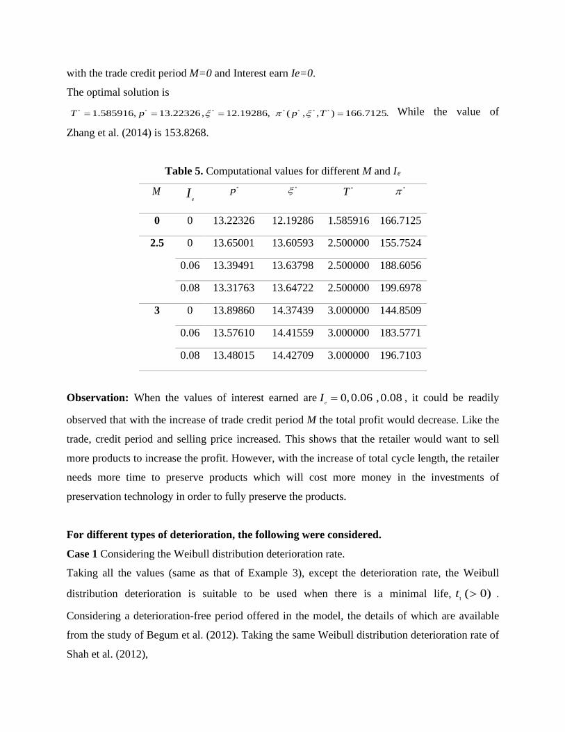
with the trade credit period M=0 and Interest earn Ie=0.
The optimal solution is
* * * * * * *1.585916, 13.22326, 12.19286, ( , , ) 166.7125.T p p Tξ π ξ= = = = While the value of
Zhang et al. (2014) is 153.8268.
Table 5. Computational values for different M and Ie
M eI
*p *ξ *T *π
0 0 13.22326 12.19286 1.585916 166.7125
2.5 0 13.65001 13.60593 2.500000 155.7524
0.06 13.39491 13.63798 2.500000 188.6056
0.08 13.31763 13.64722 2.500000 199.6978
3 0 13.89860 14.37439 3.000000 144.8509
0.06 13.57610 14.41559 3.000000 183.5771
0.08 13.48015 14.42709 3.000000 196.7103
Observation: When the values of interest earned are 0,0.06 ,0.08eI = , it could be readily
observed that with the increase of trade credit period M the total profit would decrease. Like the
trade, credit period and selling price increased. This shows that the retailer would want to sell
more products to increase the profit. However, with the increase of total cycle length, the retailer
needs more time to preserve products which will cost more money in the investments of
preservation technology in order to fully preserve the products.
For different types of deterioration, the following were considered.
Case 1 Considering the Weibull distribution deterioration rate.
Taking all the values (same as that of Example 3), except the deterioration rate, the Weibull
distribution deterioration is suitable to be used when there is a minimal life, 1 ( 0)t > .
Considering a deterioration-free period offered in the model, the details of which are available
from the study of Begum et al. (2012). Taking the same Weibull distribution deterioration rate of
Shah et al. (2012),
( ) 1( )t t βθ αβ γ −
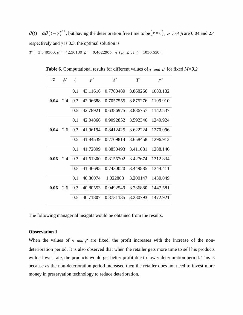
= − , but having the deterioration free time to be ( )1tγ = , andα β are 0.04 and 2.4
respectively and γ is 0.3, the optimal solution is * * * * * * *3.349560, 42.56130, 0.4622905, ( , , ) 1056.650T p p Tξ π ξ= = = = .
Table 6. Computational results for different values of andα β for fixed M=3.2
α β 1t *p *ξ *T *π
0.04 2.4
0.1 43.11616 0.7700489 3.868266 1083.132
0.3 42.96688 0.7057555 3.875276 1109.910
0.5 42.78921 0.6386975 3.886757 1142.537
0.04 2.6
0.1 42.04866 0.9092852 3.592346 1249.924
0.3 41.96194 0.8412425 3.622224 1270.096
0.5 41.84539 0.7709814 3.658458 1296.912
0.06 2.4
0.1 41.72899 0.8850493 3.411081 1288.146
0.3 41.61300 0.8155702 3.427674 1312.834
0.5 41.46695 0.7430020 3.449885 1344.411
0.06 2.6
0.1 40.86074 1.022808 3.200147 1430.049
0.3 40.80553 0.9492549 3.236880 1447.581
0.5 40.71807 0.8731135 3.280793 1472.921
The following managerial insights would be obtained from the results.
Observation 1
When the values of andα β are fixed, the profit increases with the increase of the non-
deterioration period. It is also observed that when the retailer gets more time to sell his products
with a lower rate, the products would get better profit due to lower deterioration period. This is
because as the non-deterioration period increased then the retailer does not need to invest more
money in preservation technology to reduce deterioration.

Observation 2
When the values of α is fixed, increasing β and the non-deterioration period 1t will increase
the total profit. However, the total cycle time, as well as the selling price of the products will
decrease with the increase of non-deterioration period together with β .
Case 2 Considering variable deterioration rate.
Taking all the values (same as that of Example 3), except the deterioration rate; also taking the
same time varying deterioration rate of Dye et al. (2012) as ( ) 0.2 0.1t tθ = + , and adapting it to
the model shows that the optimal solution is * * * * * * *3.00, 41.86581, 0.5119012, ( , , ) 1190.987T p p Tξ π ξ= = = = .
8. Sensitivity Analysis
Sensitivity analysis was executed on the optimal result for the given data set (example 3 from
the numerical example) in order to study the influence of under or overestimation of the
inventory system factors on the optimal values of the cycle length (T*), preservation cost ( *ξ ),
selling price (p*), initial stock (S*), maximum shortage (R*), along with the maximum profit ( *π
) of the system. The percentage variations in the aforementioned optimal values were taken as
processes of sensitivity. The analysis was carried out by changing the key parameters from -20%
to +20%, one parameter at a time and keeping all other parameter fixed, the result shown in table
7.
Table 7. Sensitivity analysis with respect to different parameters
Parameter % Change in parameters
% Change in π ∗ S ∗ R∗ p∗
ξ ∗ T ∗
b
-20 82.35 15.62 -1.82 18.62 1.99 0 -10 35.94 7.6 -0.26 8.28 0.9 0 10 -28.43 -7.22 -0.84 -6.77 -0.92 0 20 -51.22 -14.1 -2.65 -12.42 -1.78 0
a
-20 -78.32 -33.51 -22.8 -14.82 -1.7 0.72 -10 -42.87 -17.2 -10.89 -7.45 -1.01 0 10 50.35 17.58 9.78 7.45 0.9 0 20 108.2 35.47 18.6 14.9 1.7 0
pC
-20 9.3 4.6 4.19 -1.47 -15.95 0 -10 4.51 2.18 2.09 -0.72 -7.59 0

From table 7, the following observations were found.
10 -4.27 -1.99 -2.09 0.69 6.95 0 20 -8.34 -3.82 -4.17 1.36 13.37 0
1c
-20 25.81 13.39 -15.54 -3.4 19.6 0 -10 12.27 6.57 -7.33 -1.64 9.4 0 10 -11.13 -6.29 6.51 1.53 -8.78 0 20 -21.23 -12.28 12.28 2.94 -17.06 0
2c
-20 0.22 -0.25 0 -0.06 -0.19 0 -10 0.11 -0.12 0 -0.03 -0.09 0 10 -0.11 0.12 0 0.03 0.09 0 20 -0.21 0.24 0 0.06 0.19 0
3c
-20 1.91 -2.21 10.07 -0.53 -1.69 0 -10 0.91 -1.04 4.79 -0.25 -0.8 0 10 -0.82 0.94 -4.36 0.22 0.72 0 20 -1.58 1.8 -8.36 0.42 1.38 0
1a
-20 0.04 0 0 0 25 0 -10 0.04 0 0 0 11.11 0 10 0 0 0 0 -9.09 0 20 0.1 0 0 0 -16.67 0
θ
-20 -13.36 -9.69 2.27 1.98 -29.99 0 -10 -6.13 -4.56 1.02 0.9 -14.34 0 10 5.25 4.1 -0.83 -0.76 13.26 0 20 9.8 7.81 -1.5 -1.41 25.63 0
δ
-20 3.44 -3.38 20.08 -0.67 -2.43 0 -10 1.57 -1.55 9.12 -0.31 -1.12 0 10 -1.34 1.33 -7.7 0.27 0.97 0 20 -2.49 2.48 -14.29 0.5 1.81 0
OC
-20 9.55 0 0 0 0 0 -10 4.78 0 0 0 0 0 10 -4.78 0 0 0 0 0 20 -9.55 0 0 0 0 0
1t
-20 -2.67 0.75 -0.61 0.41 1.08 0 -10 -1.34 0.37 -0.3 0.21 0.55 0 10 1.35 -0.36 0.29 -0.21 -0.56 0 20 2.7 -0.7 0.57 -0.41 -1.12 0
eI
-20 -4.17 -1.36 1.2 0.31 -0.35 0 -10 -2.09 -0.67 0.6 0.15 -0.17 0 10 2.1 0.67 0.59 -0.15 0.17 0 20 4.2 1.33 1.18 -0.3 0.34 0
M
-20 2.28 -21.26 -12.52 -2.33 -13.29 -20 -10 1.64 -10.56 -6.23 -1.14 -6.59 -10 10 -2.34 10.35 6.13 1.11 6.47 10 20 -5.2 20.41 12.11 2.2 12.82 20

Observations 1
When the value of the parameters p 1 2 3b ,c ,c ,c , c , , Mδ , decreases and the value of the
parameters 1, , , ea t Iθ increases, the optimum total profit function π ∗ decreases. It is observed that
when the replenishment cost per order increases, the values of * *, pξ will increase while the
total profit π ∗ decreases. The result is analogous to the study of Zhang et al. (2014). This
indicates that if the replenishment cost per order becomes higher, the enterprise will try to
lengthen the replenishment cycle as well as ordering more quantity; this will result in more time
to recover the cost of preservation technology. In order to increase profit, it is necessary for the
enterprise to increase the selling price of goods.
Observations 2
S ∗ increases when the value of the parameters b , δ , 1t , pc , 1c decreases and a , 2c , 3c ,θ , eI , M
increases while S ∗ decreases. Moreover, there is no effect on S ∗ if the value of the parameters
O C , 1a changes. The retailer would want to store more products when the cost of purchasing is
available at a lower rate. Consequently, when the manufacturer gives more significant trade
credit period to retailers, the retailers would tend to increase the product inventory in order to
attract more buyers and sell more products.
Observations 3
R∗ increases when the value of the parameters θ , eI , δ , pc , 3c decreases and a , 1c , 1,b t , M
increases while R∗ decreases. Moreover, there is no effect on R if the value of the parameters
OC , 1a , 2c changes. It is observed that with the increase in δ , the amount of shortages
decreases and when it approaches infinity, then there will be no shortages. This means that the
optimal value of R* will be zero. The amount of shortages increases when the value of holding
cost increases which is analogous to the study by Li et al. (2018).
Observations 4
p∗ increases when the value of the parameters b , θ , 1a ,eI , tc decreases and b , 1, ,eI t θ
increases while p∗ decreases. Moreover, there is no effect on p∗ if the value of the parameters
OC , 1a changes, but there is a proportional relationship between p∗ and the value of the
parameters a , δ , pc , 2c , 3c , 1 ,c M . However, when the selling price increases, the retailer
would tend to sell more products so that the total cycle time will be longer and reduce the
shortage in order to get maximum profit. When purchase cost increases, then optimal total profit
(π ∗ ) and shortage (R*) decreases together with is the increase in selling price. The result of
which is analogous to the study by Tiwari et al. (2018).
Observations 5
ξ ∗ increases when the value of the parameters a , b 1t , 1c increases and a , b 1t , 1c , increases
while ξ ∗ decreases. Moreover, there is no effect on R if the value of the parametersOC changes,
but there is a proportional relationship between p∗ and the value of the parameters a , δ , pc , 2c ,
3c , ,eI ,M θ . When the value of the simulation coefficient 1a increases, then the value of
preservation investment decreases. It is also observed that the investment on preservation
technology lengthened the non-deterioration period and reduced the deterioration, which is
observed in the study by Li et al. (2018).
Observations 6
T ∗ increases when the value of the parameters ,a b decreases. Moreover, there is no effect on
R when the value of the parameters 1 2 3 1 1, , , , c , , , , ,p eOC a c c c I t θ δ changes and there is a
proportional relationship between total cycle length and trade credit period. This means that
when the retailer gets more trade credit period, the retailer would lengthen the cycle length.

9. Conclusions and Comments
In this study, we have derived a deteriorating inventory model with price dependent demand,
partial backlogging and trade credit considering preservation technology for perishable goods. It
has been shown that the investment in preservation technology has lengthened the freshness of
goods. Furthermore, to increase competitiveness, this model also takes into account of credit
financing as a strategy that benefits retailers. We have derived the optimal cycle length, optimal
selling price and investments in preservation technology in order to maximize the total profit.
Numerical analysis is carried out to show the importance of preservation technology investment
and trade credit policy. Finally, with the help of MATLAB 2017a software, it is shown
graphically that the profit function is concave, and sensitivity analysis is done using Lingo17.
The study provides insight for managers to make smart decisions especially in the scope of
applying preservation technology and credit financing. The main limitation in the study is the
assumption of fixed trade-credit period. For future research, this paper can be extended to
consider some features such as probabilistic demand rate, variable trade-credit period, variable
deterioration rate, quantity discounts, and multiple products.
References
[1] Aggarwal, S. P., and Jaggi, C. K., Ordering policies of deteriorating items under
permissible delay in payments. Journal of the Operational Research Society 46(5) (1995)
658-662.
[2] Begum, R., Sahoo, R. R. and Sahu, S. K., A replenishment policy for items with price-
dependent demand, time-proportional deterioration and no shortages. International
Journal of Systems Science 43(5) (2012) 903-910.
[3] Chen, S. C. and Teng, J. T., Inventory and credit decisions for time-varying deteriorating
items with up-stream and down-stream trade credit financing by discounted cash flow
analysis. European Journal of Operational Research 243(2) (2015) 566-575.
[4] Dye, C. Y. and Hsieh, T. P., An optimal replenishment policy for deteriorating items with
effective investment in preservation technology. European Journal of Operational
Research 218(1) (2012) 106-112.
[5] Dye, C. Y., The effect of preservation technology investment on a non-instantaneous
deteriorating inventory model. Omega 41(5) (2013) 872-880.

[6] Dey, B. K., Sarkar, B., Sarkar, M. and Pareek, S. An integrated inventory model involving
discrete Setup cost reduction, variable safety factor, selling price dependent demand, and
investment. RAIRO-Operations Research 53 (2019) 39-57.
[7] Goyal, S. K., Economic order quantity under conditions of permissible delay in
payments. Journal of the Operational Research Society 36(4) (1985) 335-338.
[8] Hsieh, T. P., and Dye, C. Y., A production–inventory model incorporating the effect of
preservation technology investment when demand is fluctuating with time. Journal of
Computational and Applied Mathematics 239 (2013) 25-36.
[9] He, Y. and Huang, H., Optimizing inventory and pricing policy for seasonal deteriorating
products with preservation technology investment. Journal of Industrial Engineering 2013
(2013) Article ID 793568 7 pages, https://doi.org/10.1155/2013/793568.
[10] Jaggi, C. K., Tiwari, S. and Goel, S. K., Credit financing in economic ordering policies for
non-instantaneous deteriorating items with price dependent demand and two storage
facilities. Annals of Operations Research 248(1-2) (2017) 253-280.
[11] Liu, G., Zhang, J. and Tang, W., Joint dynamic pricing and investment strategy for
perishable foods with price-quality dependent demand. Annals of Operations Research
226(1) (2015) 397-416.
[12] Lu, L., Zhang, J. and Tang, W., Optimal dynamic pricing and replenishment policy for
perishable items with inventory-level-dependent demand. International Journal of Systems
Science 47(6) (2016) 1480-1494.
[13] Li, G., He, X., Zhou, J. and Wu, H., Pricing, replenishment and preservation technology
investment decisions for non-instantaneous deteriorating items. Omega 84 (2018) 114-
126.
[14] Mishra, V. K., Controllable deterioration rate for time-dependent demand and time-
varying holding cost. Yugoslav Journal of Operations Research 24(1) (2014) 87-98.
[15] Mishra, V. K., An inventory model of instantaneous deteriorating items with controllable
deterioration rate for time dependent demand and holding cost. Journal of Industrial
Engineering and Management 6 (2) (2013) 495-506.
[16] Mashud, A., Khan, M., Uddin, M and Islam, M., A non-instantaneous inventory model
having different deterioration rates with stock and price dependent demand under partially
backlogged shortages. Uncertain Supply Chain Management 6(1) (2018) 49-64.
[17] Mishra, U., Aguilera, J.T., Tiwari, S. and Barron, L. E. C., Retailer’s Joint Ordering,
Pricing, and Preservation Technology Investment Policies for a Deteriorating Item under
Permissible Delay in Payments. Mathematical Problems in Engineering 5 (2018) 1-14
[18] Nobil A. H., C ́ardenas–Barr ́on L.E. and Nobil, E., Optimal and simple algorithms to
solve integrated procurement-production-inventory problem without/with shortage.
RAIRO-Operations Research 52 (2018) 755-778.
[19] Nobil, A. H., Kazemi, A. and Taleizadeh, A. A., Single-machine lot scheduling problem
for deteriorating items with negative exponential deterioration rate. RAIRO-Operations
Research 53(4) (2019) 1297-1307.
[20] Nobil, A. H., Kazemi, A. and Taleizadeh, A. A., Economic lot-size problem for a cleaner
manufacturing system with warm-up period. RAIRO-Operations Research (2019)
https://doi.org/10.1051/ro/2019056
[21] Pandey, R., Singh, S., Vaish, B. and Tayal, S., An EOQ model with quantity incentive
strategy for deteriorating items and partial backlogging. Uncertain Supply Chain
Management 5(2) (2017) 135-142.
[22] Pal, B., Optimal production model with quality sensitive market demand, partial
backlogging and permissible delay in payment. RAIRO-Operations Research 52 (2018)
499-512.
[23] Palanivel, M. and Uthayakumar, R. An inventory model with imperfect items, stock
dependent demand and permissible delay in payments under inflation. RAIRO-Operations
Research 50(3) (2016) 473-489.
[24] Shah, N. H., Soni, H. N. and Patel, K. A., Optimizing inventory and marketing policy for
non-instantaneous deteriorating items with generalized type deterioration and holding cost
rates. Omega 41(2) (2013) 421-430.
[25] Shaikh, A. A., Mashud, A. H. M., Uddin, M. S. and Khan, M. A. A., Non
instantaneous deterioration inventory model with price and stock dependent demand for
fully backlogged shortages under inflation. International Journal of Business
Forecasting and Marketing Intelligence 3(2) (2017) 152-164.
[26] Sett, B. K., Sarkar, B., and Goswami, A., A two-warehouse inventory model with
increasing demand and time varying deterioration. Scientia Iranica, 19(6) (2012) 1969-
1977.

[27] Sarkar B. and Sarkar S, An improved model with partial backlogging, time varying
deterioration and stock-dependent demand. Economic Modelling 30 (2013) 924-932.
[28] Singh, S., Khurana, D. and Tayal, S., An economic order quantity model for deteriorating
products having stock dependent demand with trade credit period and preservation
technology. Uncertain Supply Chain Management 4(1) (2016) 29-42.
[29] Teng, J. T., Min, J. and Pan, Q., Economic order quantity model with trade credit
financing for non-decreasing demand. Omega 40(3) (2012) 328-335.
[30] Tiwari, S., Cárdenas-Barrón, L. E., Khanna, A. and Jaggi, C. K., Impact of trade credit and
inflation on retailer's ordering policies for non-instantaneous deteriorating items in a two-
warehouse environment. International Journal of Production Economics 176 (2016) 154-
169.
[31] Tiwari, S., Cárdenas-Barrón, L. E., Goh, M. and Shaikh, A.A. Joint pricing and inventory
model for deteriorating items with expiration dates and partial backlogging under two-
level partial trade credits in supply chain. International Journal of Production Economics
200 (2018) 16-36.
[32] Tiwari, S., Wee, H. M. and Sarkar, S., Lot-sizing policies for defective and deteriorating
items with time-dependent demand and trade credit. European Journal of Industrial
Engineering, 11(5) (2017), 683-703.
[33] Tsao, Y. C. and Sheen, G. J., Dynamic pricing, promotion and replenishment policies for a
deteriorating item under permissible delay in payments. Computers & Operations
Research 35(11) (2008) 3562-3580.
[34]
[35]
Yang, C. T., Dye, C. Y. and Ding, J. F., Optimal dynamic trade credit and preservation
technology allocation for a deteriorating inventory model. Computers & Industrial
Engineering 87 (2015) 356-369.
Zhang, J., Bai, Z. and Tang, W., Optimal pricing policy for deteriorating items with
preservation technology investment. Journal of Industrial & Management Optimization
10(4) (2014) 1261-127.

Appendix A:
From equation (9):
( ) ( ) ( )( ){ }3 2
2
2
log 1
Which implies that
1 1
which can be written in the form( )
RD
a bpR I T T t
t T e
t T f D
δ
δδ
δ
−= − = + −
= + −
= +
(A.1)
( )
( )( ) { }
( ) ( )( )
( )( ) { }
( )( )
1
2
( ( ) )1
21
1 1 223
Now putting the value of in equation (23) then it reduces to
( )( ) log(1 ( ( )))
( )1 log(1 ( ( )))
( )1
1 2, ,
m T f D t
t
a bpp a bp T f D T T f D A
a bp a bpc a bp t e T T f Dm
a bpa bp tc St
mp TT
θ ξ
δδ
δθ ξ δ
θ ξπ ξ
+ −
− − + + + − − − − − −
− + − + + − − −
−−− − −
=
( )( ) ( ) ( )( )
( ) ( )( ) ( )( )
( ) ( ) ( )( ){ } ( )( )
( )( ) ( )( )
1( )1
2 2
23
( )
R ( ) 1 ( ) log 1 ( )
( )( ) log 1 ( )
2( )
log 1 ( )
m T f D t
e
e
e m T f D t
D Dc T T f D T T f D T T f D
c a bp pI a bp T f DT T f D T T f D
pI a bp T f DT T f D
θ ξ θ ξ
δ δδ δ
δ δδ
δδ
+ −
+ + − −
+ − − − + − − + − − −
− − +− − − − − − + +
− +
+ − −
( )( ) { }
( ) ( )( )
( )( ) { }
( )( )
( )( ) ( ) ( )( )
( ) ( )( )
1
1
( ( ) )1
2( )1
1 1 122
2 2
( )( ) log(1 ( ))
( )1 log(1 ( ))
( )1 ( )
1 2
R ( ) 1 ( ) log(1
m T f D t
m T f D t
a bpp a bp T f D f D A
a bp a bpc a bp t e f Dm
a bpa bp tc St e m T f D t
mT D Dc f D f D f
θ ξ
θ ξ
δδ
δθ ξ δ
θ ξθ ξ
δ δδ δ
+ −
+ −
− − + + − − − − −
− + − + − − −−
− − − + + − − = − − − −
{ }
( ) ( ) { }{ } ( )( )
( )( ) { }
23
( ))
( )( ) log(1 ( ))
2( )
log(1 ( ))
1 ( , , ) ,since D a bp
e
e
D
c a bp pI a bp T f Df D f D
pI a bp T f Df D
G p TT
δ δδ
δδ
ξ
−
− − + − − − + +
− +
−
= = −(A.2)

{ }
{ }2 1
2 1
2
2 2
( )( )1
( )( )2
( )( ) log(1 ( )) , 0
, 0
( )( ) 1( )
( )1 1( ) . . .
Differentiate with respect to we ha e
( )( )
v
m t t
m t t
a bp SR SRSR p a bp t T t
OCOC A
a bpPC c a bp t em
dmPC c a
X
bp ed mm
θ ξ
θ ξ
δδ ξ ξ
ξ
θ ξ
ξξ ξ θ ξθ
ξ
ξ
−
−
− ∂ ∂ = − + + − = = ∂ ∂ ∂
= =∂
−= − + −
∂= − − +
∂2 1
2 1 2 1
2 12 1 1
( )( )2 1
( )( ) ( )( )1 2 1
( )( )2( )( )2
1 2 1 2 1 12 2
( )( ).
1( ) . ( )( )
.( ) ( ) 1 ( ) ( )( )
m t t
m t t m t t
m t tm t t a
dme t td
c a bp a e e t tm
PC ec a bp a e t t t t e c a bp am
θ ξ
θ ξ θ ξ
θ ξθ ξ ξ
ξθξ
θ ξ
θξ θ ξ
−
− −
−− −
−
= − − −
∂ = − − − − − − ∂
(A.3)
( ) ( )( ) ( )( )
( ) ( ) ( )( ){ }( ) ( ) ( )( )
2 2 2 22
2
2
23
2 2 2
2 22 2 1 1
3 2 2
2
2
R 1 log 1
0
log 1 0
log 1 , 02
0
e e
D DBC c T t T t T t
BC BC
c a bp LSC LSCLSC T t T t
pI a bp t pI a bp t E EIE T t
PTC PTCPTC T T and
δ δδ δ
ξ ξ
δ δδ ξ ξ
δδ ξ ξ
ξξ ξ
= + − − + − + −
∂ ∂= =
∂ ∂
− ∂ ∂= − − + − ⇒ = =
∂ ∂
− − ∂ ∂= + + − = =
∂ ∂
∂ ∂= ⇒ = =
∂ ∂
Differentiating with respect to " "X p shows
{ }
{ }
2 2
2
2 22
( )( ) log(1 ( )) ,
22 log(1 ( ))
a bpSR p a bp t T t
SR bbt T tp
δδ
δδ
− = − + + − ∂ = − − + − ∂
(A.4)
( ) ( )( )
( )( ) { }
( )( )( ) { }
2 1
2 1
2
2
( )1 2
2( )
1 2 2
, 0
( )1 log(1 ( ))
1 11 log(1 ( )) 0
m t t
m t t
OC OCOC Ap p
a bp a bpPC cQ c a bp t e T tm
PC PCbc t e T tp m p
θ ξ
θ ξ
δθ ξ δ
δθ ξ δ
−
−
∂ ∂= = =
∂ ∂
− −= = − + − + + −
∂ ∂
= − + − + + − ⇒ = ∂ ∂
(A.5)

{ }
{ }
( ) ( )
2 1
2 1
2( )( )1
1 1 2 12 2
2( )( )2
1 1 2 12 2 2
2 2 2 22
( ) ( ) 1 ( )( )2 ( )
1 1 ( )( ) 02 ( )
1 ( ) log(1 ( ))
m t t
m t t
a bp t a bpIHC c st e m t tm
IHC b IHCc bt e m t tp m p
a bp a bpBC c R T t T t T t
BC
θ ξ
θ ξ
θ ξθ ξ
θ ξθ ξ
δ δδ δ
−
−
− −= − − − + −
∂ ∂
= + − + − ⇒ = ∂ ∂ − − = + − − + − + −
∂ ( ) ( )2
2 2 2 22 21 ( ) log(1 ( )) 0b b BCc t T T t T tp p
δ δδ δ
∂ = − + + − + − ⇒ = ∂ ∂
(A.6)
( ) ( ) ( )( ){ }
( ) ( )( ){ }( ) ( ) ( )( )( ) ( ) ( )( )
( )( )
32 2
23
2 2 2
22 2
3 2
22 23
2
2 23 2 2
22
log 1
log 1 0
log 12
2 2log 1
2
log 12
e e
e e
e e
c a bpLSC T t T t
c bLSC LSCT t T tp p
pI a bp t pI a bp tIE T t
I a bp t I a bp tET t
p
E I bt I btT t
p
δ δδ
δ δδ
δδ
δδ
δδ
−= − − + −
∂ ∂= − − − + − ⇒ =
∂ ∂
− −= + + −
− −∂= + + −
∂
∂= − − + −
∂
(A.7)
Differentiating with respect to " "X T shows
{ }2 2
2
( )( ) log(1 ( ))
( ) ; , 0(1 ( )
a bpSR p a bp t T t
p a bpSR OCOC AT T t T
δδ
δ
− = − + + − −∂ ∂
= = =∂ + − ∂
(A.8)
{ }2 1( )( )1
2
( )( ) 1( )
( )(1 ( )
m t ta bpPC c a bp t em
c a bpPCT T t
θ ξ
θ ξ
δ
− −= − + −
−∂
=∂ + −
(A.9)

{ }
{ }
2 1
2( )( )1
1 1 2 12 2
22 2 2 2 22
2 22 2
( ) ( ) 1 ( )( ) , 02 ( )
( )(1 ( )( ) (1 ( ) log(1 ( )) 1 1
( )(1 2 ( ))1 log(1 ( ))
m t ta bp t a bp IHCIHC c st e m t tTm
c a bp a bpBC T t T t c T t T t
c a bp T t a bpBC c T tT
θ ξ θ ξθ ξ
δ δ δδ δ
δδ
δ δ
− − − ∂= − − − + − =
∂ − −
= + − − + + − + − − +
− + − −∂= − + + − −
∂{ }
( ) ( ) ( )( ){ }
( )( )( )
( ) ( ) ( )( ) ( )( )( )
32 2
32
2 22 2 3
3 22
1
log 1
111
log 12 1
,
e e e
c a bpLSC T t T t
LSC c a bpT T t
pI a bp t pI a bp t pI a bp tEIE T t
T T t
PTCPTC TT
δ δδ
δ
δδ δ
ξ ξ
−= − − + −
∂ = − −
∂ + − − − −∂
= + + − ⇒ =∂ + −
∂= ⇒ =
∂
(A.10)
Appendix B
Proof of Corollary 1
The objective function is
( )3 , ,T XpT
π ξ = (B.1)
Differentiating the equation (B.1) with respect to T,
( )3
2
, ,TXT Xp T
T Tπ ξ
∂−∂ ∂=
∂ (B.2)
Differentiating the equation (B.2) with respect to T,
( )2
22 3 2
2 3
22
2
3
2, ,T
2 2
X X X XT T T T Xp T T TTT T
X XT T XTT
T
π ξ ∂ ∂ ∂ ∂ + − − − ∂ ∂ ∂ ∂∂ =
∂∂ ∂
− +∂∂=
(B.3)
From equation (B.3) we observed that

( )2 3
2
, ,T0
pT
π ξ∂<
∂,
which means 2
222
3 2 2 3
2
2 3 2
2 2 1 2 20 , 0
1 2 2
X XT T X X X XTTT TT T T T
X X XT TT T T
∂ ∂− + ∂ ∂∂∂ < ⇒ − + <
∂∂∂ ∂
⇒ + <∂∂
(B.4)
Proof of Corollary 2
For any fixed ξ and T, the second order derivative of the objective function 3( , , )p Tπ ξ with
respect to the decision variables p is
{ } ( )( )22 32 2
2 2 22
( , , ) 1 22 log(1 ( )) log 1 02
e eI bt I btp T bbt T t T tTp
π ξ δ δδ δ
∂= − + + − − + + − <
∂ (B.5)
Which implies that,
{ } ( )( )
( )( )
( )( )
( )( )
22 2
2 2 2
222 2 2
222 2 2
2 22
2
22 log(1 ( )) log 1 0 , since is the total cycle length2
244 log 1
24 log 1 4
( 4)log 1
2 4
e e
ee
ee
e
e
I bt I btbbt T t T t T
I tt T t I t
I tT t I t t
I t tT t
I t
δ δδ δ
δδ δ
δδ δ
δδ
+ + − − + + − >
⇒ + + + − >
⇒ + + − > −
−
⇒ + − >+
W
(B.6)
Now the mixed derivatives with respect to the decision variables
2 12 1
2 1
2 12 1
( )( )( )( )
1 2 12 3
( )( )1 1 2 12 2
( )( )( )( )
1 2 1
2 3
2
( )( )( , , ) 1
2 1 1 ( )( )( )
( ) (( )
( , , ) 1
m t tm t t
m t t
m t tm t t
ea bc e t tmp T
p T b bc a e t tmm
eca a bp e t tm
p TT T
θ ξθ ξ
θ ξ
θ ξθ ξ
θ ξπ ξξ
θ θ ξθ ξ
θ ξπ ξ
ξ
−−
−
−−
+ − −
∂ = ∂ ∂ + − −
− − − −
∂= −
∂ ∂2 1 2 1( )( ) ( )( )
2 2 2 2
1 1
2 1
)
2( ) ( )1 2 1( ) ( )
1( ) ( )
( )
m t t m t ta bp a bp e em m
c aa bp t t
m
θ ξ θ ξ
θθ ξ θ ξ
θ ξ
− −
−
− − − − + − − + −
( )( )( ) ( )
{ } { }
2 1 2 1
2 1 2 1
( ) ( )1 2 12 3
( )( ) ( )( )2 11 2 12 2
1 1 ( ).( , , ) 1
( )2 1 ( )( ) 1( )( )
m t t m t t
m t t m t t1
a bc e e t tmp T
p T t tc ba e m t t e
mm
θ ξ θ ξ
θ ξ θ ξ
θ ξπ ξξ
θ ξθ ξθ ξ
− −
− −
− − − −
∂ = ∂ ∂ − − + − + −
{ } ( )( )( )
{ }
{ }
( ) ( )
2 1
2 1
( )1
2 2
2
( )( )21 1 2 12 2
2 3
22 2 2 22
1 1( 2 )( 2 ) log(1 ( ))
1 log(1 ( ))
1 1 ( )( )2 ( )
( , , ) 11 ( ) log(1 ( ))
m t t
m t t
t ema bpa bp t T t bc
T t
bc bt e m t tm
p Tb bp T T c t T T t T t
θ ξ
θ ξ
θ ξδ
δδ
δ
θ ξθ ξ
π ξδ δ
δ δ
−
−
+ − − − + + − + + + −
− + − + − −
∂= − ∂ ∂ − + + − + −
( ) ( )( ){ } ( )
( ) ( )( )
223
2 2
22
2 22 2
32
2log 1
22
log 1
( 2 ) 1 log(1 ( ))1 ( ) 1 ( )1
111 ( )
e
e
e
I a bp tc bT t T t
I a bp tT t
a bp b bbc c T tT t T t
T Ic b
T t
δ δδ
δδ
δ δδ δ δ δ
δ
−+ − − + − − + − + −
− + − − + + − + + − + − +
+ − + + −
( ) 2
2
21 ( )
a bp tT tδ
− + −
(B.7)
{ }
( )( )( ) { }
{ }
( ) ( )
2 1
2 1
2 2
( )1 2
( )( )21 1 2 12 3 2 2
2 2 2 22
( 2 )( 2 ) log(1 ( ))
1 11 log(1 ( ))
1 1 ( )( )2( , , ) 1 ( )
1 ( ) log(1 ( ))
m t t
m t t
a bpa bp t T t
bc t e T tm
bc bt e m t tp T m
T p T b bc t T T t T t
θ ξ
θ ξ
δδ
δθ ξ δ
θ ξπ ξ θ ξ
δ δδ δ
−
−
−− + + − +
+ − + + −
− + − + − − ∂ = −
∂ ∂ − + + − + −
+ ( ) ( )( ){ } ( )
( ) ( )( )
( )( )22
2
23
2 2
223
2 2
22
b2 log 11 ( )1
( 2 )111 ( ) 1 ( )
2log 1
22
log 1
e
e
e
ca bc bp T tT t
T I a bp tc b
T t T t
I a bp tc bT t T t
I a bp tT t
δδ δ
δ δ
δ δδ
δδ
+ − − + − + − + − − − − + − + − − − − + − − + − + −
2 12 1
2 1 2 1
( )( )( )( )
1 2 1
2 3( )( ) ( )( )
2 2 2 2
1 1
2 1
( ) ( )( )
( , , ) 1 2( ) ( )1 2 1( ) ( )
( ) ( )( )
m t tm t t
m t t m t t
eca a bp e t tm
p T a bp a bp e eT T m mc a
a bp t tm
θ ξθ ξ
θ ξ θ ξ
θ ξπ ξ
ξ θθ ξ θ ξ
θ ξ
−−
− −
− − − − − ∂ − − = − − − + ∂ ∂ − + −
(B.8)


