Pricing of Discrete
Barrier Options
�
Kellogg College
University of Oxford
A thesis submitted in partial fulfilment of the requirementsfor the MSc in
Mathematical Finance
October 22, 2003

“Pricing of Discrete Barrier Options”
MSc in Mathematical Finance
Trinity 2003
Abstract
This study addresses the pricing of discrete barrier options using analytical methods
and numerical simulations. For discrete barrier options, the asset price is only monitored at
instantsti = iT/m, whereT is the expiration date andm − 1 is the number of monitoring
points (i = 1, 2, ..., m− 1). The analytical solution for discrete barrier options involvesm-
dimensional integrals, which are not analytically tractable for options with a high number
of monitoring points (m > 5). The use of numerical procedures for pricing discrete barrier
options becomes increasingly difficult at even higher numbers of monitoring points, e.g.
m ≈ 100. In this case, it is convenient to perform an asymptotic expansion that becomes
exact in the limit as the number of monitoring points goes to infinity. Broadie et al. [1]
have derived a continuity correction for discrete barrier options that satisfies this condition.
We show that the continuity correction for single barrier options with discrete monitoring
can also be derived within the framework of matched asymptotic expansions. This method
can be extended to derive an asymptotic expression for double barrier options with discrete
monitoring.
Contents
1 Introduction 1
2 Barrier options with continuous monitoring 4
2.1 Model . . . . . . . . . . . . . . . . . . . . . . . . . . . . . . . . . . . . . 4
2.2 Time-independent barrier option . . . . . . . . . . . . . . . . . . .. . . . 8
2.3 Time-dependent barrier option . . . . . . . . . . . . . . . . . . . . .. . . 11
2.4 Down-and-Out call option revisited . . . . . . . . . . . . . . . . .. . . . . 13
2.5 Double Barriers . . . . . . . . . . . . . . . . . . . . . . . . . . . . . . . . 14
3 Pricing of discrete barrier options 16
3.1 Model and solution . . . . . . . . . . . . . . . . . . . . . . . . . . . . . . 16
3.2 Discrete down-and-out call option revisited . . . . . . . . .. . . . . . . . 19
3.3 Continuity correction for discrete barrier options . . .. . . . . . . . . . . 20
4 Asymptotic expansion for single barrier options 25
4.1 General remarks . . . . . . . . . . . . . . . . . . . . . . . . . . . . . . . . 25
4.2 Van Dyke’s matching principle . . . . . . . . . . . . . . . . . . . . . .. . 29
4.3 Matched asymptotic expansions . . . . . . . . . . . . . . . . . . . . .. . 31
5 Asymptotic expansion for double barrier options 36
5.1 Matched asymptotic expansions . . . . . . . . . . . . . . . . . . . . .. . 36
6 Conclusion and Outlook 42
A Useful integral 43
i
Chapter 1
Introduction
Barrier options are one of the oldest and most popular examples of the so-called "exotic"
options that have been proposed and analysed over the last three decades. Unlike many oth-
ers of these second generation derivatives, barrier options are heavily traded instruments.
The payoff of a barrier option depends on the path of the underlying asset through its op-
tion life. The option is activated or extinguished wheneverthe underlying asset price hits a
barrier for the first time. For example, only if the underlying asset price reaches the barrier
before maturity a down-and-in call option gives the option holder the payoff of a European
call option at maturity. Other types of barrier options are the down-and-out, up-and-in and
up-and-out call/put option, whose payoffs are self-explanatory. The extension of single
barrier options to double barrier options has also become popular in OTC markets. Alter-
native barrier option contracts have been proposed by Davydov et al. [2]. They designed
the so-called barrier step options, which regularize the knockout of the option by introduc-
ing a finite knockout of the option, in which the payoff of the option depends on the time
that the underlying asset price is beyond a pre-specified barrier level.
Another class of barrier options involves the nature of the barrier itself. First, we consider
the form of the barrier. Partial barrier options belong to this class of barrier options. They
are characterized by a changing barrier level from one time period of the option’s life to
another. As an example, we mention the front-end and rear-end barrier options, whose
barriers only exist at the beginning or at the end of the options life, respectively. Second,
we address the monitoring frequency of the barrier, i.e. howfrequently the barrier condi-
tion is checked. Most models assume continuous monitoring of the barrier. However, in
1
practice, most of the barrier options are monitored at discrete instants, e.g. daily or weekly.
Numerical investigations have shown that discrete and continuous barrier options can have
significantly different prices even for daily monitoring (see [3]). The pricing of continuous
and discrete barrier options is the subject of this work.
Why should an investor use a barrier option rather than a plain vanilla option? One reason is
that barrier options are generally cheaper than standard options, since the asset price has to
satisfy an additional condition for the option holder to receive the payoff. The premium for
a barrier option can be significantly smaller for high volatile assets. Thus, barrier options
prevent investors from paying for scenarios that they feel are unlikely to occur. Barrier
options may also match hedging needs more closely than standard options. A drawback in
using barrier options is the possibility of triggered barrier events around popular levels as a
consequence of a manipulation of the underlying asset price, e.g. by inducing an increased
volatility of the asset.
Various approaches for the valuation of continuous barrieroptions have been developed
and published. Merton [4] has first derived a formula for a down-and-out call option. Dou-
ble barrier options and their extension to curved boundaries are discussed by Kunitomo et
al. [5] using a probabilistic approach. Geman et al. [6] and Pelsser [7] used the Laplace
transform to solve the Black-Scholes equation for various types of barrier options. Hui et
al. [8, 9] has exploited the Fourier formalism in order to obtain an analytical solution for
a double barrier option. He has also obtained analytical solutions for the front-end and
rear-end barrier options.
We have a completely different situation for discretely monitored barrier options. In gen-
eral, the price of a discrete barrier option can be expressedin terms of anm-dimensional
integral over them-dimensional multivariate normal distribution function (m − 1 is the
number of monitoring points). Unfortunately, this expression is not analytically tractable
for options with a high number of monitoring points (m > 5). To deal with these dif-
ficulties various numerical procedures and asymptotic expansions have been developed
[1, 10, 11, 12].
The outline of this work is as follows. In chapter 2, we discuss continuous barrier options
and present a method for solving the Black-Scholes equationof a down-and-out call option.
The results are compared with a Monte Carlo simulation. In chapter 3, we present a pricing
formula for discrete barrier options. The analytical solution is compared with the outcome
2

of a Monte Carlo simulation for an option with a single barrier at one instant. Furthermore,
we consider the continuity correction for discrete barrieroptions as introduced by Broadie
et al. [1]. Again, the analytical solution for the asymptotic behaviour is compared with the
results of a Monte Carlo simulation. In chapter 4, we performan asymptotic expansion of
the discrete down-and-out option in the limit of a high number of monitoring events using
the method of matched asymptotic expansions. We show that the continuity correction for
single barrier options can be derived within this framework. Finally, we apply this method
to discrete double barrier options to derive an asymptotic result for largem in chapter 5.
3
Chapter 2
Barrier options with continuous
monitoring
The purpose of this chapter is to review the pricing of a continuously monitored barrier
option. First, we derive the price of a simple barrier optionand compare the result with a
Monte Carlo simulation. Furthermore, we discuss differentapproaches for the pricing of
more complicated barrier options.
2.1 Model
Throughout this work we consider the Black-Scholes framework, in which the price of an
option is given by an expectation value of the discounted final payoff of the option with
respect to the risk-neutral probability measure. In the Black-Scholes world, the underlying
asset priceSt follows a geometric Brownian motion
dS
S= rdt + σdWt , (2.1)
wherer is the risk-free rate,σ is the volatility andWt is a standard Wiener process. The
solution of Eq.(2.1) can be written as
St = S0 exp{
(r − σ2/2)t + σWt
}
. (2.2)
In the following, we concentrate on single barrier options.The barrier may be constant
4
over time, i.e. a time-independent barrier, or may vary withtime, i.e. a time-dependent
barrier. We mention the continuously monitored barrier option as an example for a time-
independent barrier and the discretely monitored barrier option and the front-end barrier
option as examples for a time-dependent barrier. LetBt denote the level of the barrier at
time t. The first time when the asset price reaches the barrier is called the first exit time or
stopping time of the processSt. The first exit time is defined by
τ(Bt, St) = inf {t ≥ 0; St ≤ Bt} . (2.3)
The value of a barrier option can now be expressed as a function of the first exit time. For
example, the price of a continuously monitored down-and-out call option in the risk-neutral
measure Q is given by the expectation value of the discountedpayoff of the option
V (S, Bt′ , t) = EQ
(
e−r(T−t) max(ST − K, 0)1τ(Bt′ ,St′)>T
)
, (2.4)
whereS = S0. We have also introduced the characteristic function1τ(Bt,St)>T given by
1τ(Bt,St)>T =
{
1 τ(Bt, St) > T
0 otherwise. (2.5)
All other types of barrier options, e.g. up-and-in put option etc., can be represented sim-
ilarly. In the next step, we change the probability measure using the Girsanov theorem.
The expectation of the payoff with respect to the measureQ can be transformed to an ex-
pectation with respect to some measureQ⋆ by the use of the Radon-Nykodym derivative
dQ/dQ⋆ [13]. Thus, we have
EQ
(
eσWT −σ2T/21τ(Bt,St)>T
)
= EQ⋆
(
dQ
dQ⋆eσWT −σ2T/2
1τ(Bt,St)>T
)
. (2.6)
Here, we have restricted our consideration to the first term in (2.4) and inserted Eq.(2.2) for
the underlying asset priceST . To simplify the calculations, we change the measure in such
a way that it satisfies the following relation
EQ
(
eσWT −σ2T/21τ(Bt,St)>T
)
= EQ⋆
(
1τ(Bt,St)>T
)
. (2.7)
In order to satisfy this condition, the Radon-Nykodym derivative should equal
5

dQ
dQ⋆= e−σWT +σ2T/2 . (2.8)
According to Girsanov’s theorem, a change of measure leads to a change of the drift in the
underlying process. Suppose the underlying process, givenin Eq.(2.1), under the measure
Q⋆ reads as
dS
S= r⋆dt + σdW ⋆
t . (2.9)
Girsanov’s theorem relates the measureQ to the measureQ⋆. The theorem can be written
as
dQ
dQ⋆= e−
r−r⋆
σWT + (r−r⋆)2
σ2T2 . (2.10)
Now, we can apply Girsanov’s theorem to obtain the driftr⋆ of the underlying process
under the measureQ⋆ that satisfies the condition (2.8). A simple analysis shows that the
drifts r andr⋆ are related by
r⋆ = r + σ2 . (2.11)
Thus, the underlying processlnSt has the drift(r + σ2) under the measureQ⋆ instead of
r under the measureQ. The price of the down-and-out call option in terms of the measure
Q⋆ can be written as
V (S, Bt′ , t) = S EQ⋆(1ST >K,τ(Bt′ ,St′)>T ) − EQ(e−r(T−t)K1ST >K,τ(Bt′ ,St′)>T ) . (2.12)
In terms of the probability, Eq.(2.12) can be rewritten as
V (S, Bt′ , t) = SPQ⋆(ST ≥ K; τ(Bt′ , St′) > T )−e−r(T−t)KPQ(ST ≥ K; τ(Bt′ , St′) > T ) .
(2.13)
Eq.(2.13) represents the Black-Scholes price of a down-and-out call option as a function
of the probability that the asset price at expiry is larger than the strikeK and that the first
6

exit time is larger thanT with respect to the probability measurePQ⋆ and the risk neutral
measurePQ, respectively. In the following, we evaluate these probabilities for a constant
barrierBt = B. First, we insert Eq.(2.2) for the underlying asset priceSt. We obtain
V (S, B, t) = SPQ⋆(Se(r+σ2/2)T+σWT ≥ K; τ(B, St′) > T )
− e−r(T−t)KPQ(Se(r−σ2/2)T+σWT ≥ K; τ(B, St′) > T ) . (2.14)
In order to compute these probabilities, we exploit a theorem by Bielecki and Rutkowski
(see lemma 3.1.4 in [14]). Suppose that the stochastic processYt is related to a standard
Wiener processWt by Yt = Y0+νt+σWt, whereν is the drift of the process. Furthermore,
we assume that the first exit timeτ(0, Yt) is given byτ(0, Yt) = inf {t ≥ 0; Yt ≤ 0}. Then,
the theorem reads as follows:
P (YT ≥ y; τ ≥ T ) = N
(
Yt − y + ν(T − t)
σ√
T − t
)
− e−2νYt/σ2
N
(−Yt − y + ν(T − t)
σ√
T − t
)
,
(2.15)
whereN(x) is the cumulative probability distribution function for a normally distributed
variable with a mean of zero and a standard deviation of1. In the next step, we compute
the probabilities in (2.14). Applying this theorem withYt = ln(S/B), y = ln(K/B) and
ν = (r + σ2/2) for the first contribution in (2.14) andν = (r − σ2/2) for the second
contribution in (2.14) yields
V (S, B, t) = SN
(
ln(S/K) + (r + σ2/2)(T − t)
σ√
T − t
)
− B
(
S
B
)−2r/σ2
N
(
ln(B2/SK) + (r + σ2/2)(T − t)
σ√
T − t
)
+ Ke−r(T−t)N
(
ln(S/K) + (r − σ2/2)(T − t)
σ√
T − t
)
− Ke−r(T−t)
(
S
B
)1−2r/σ2
N
(
ln(B2/SK) + (r − σ2/2)(T − t)
σ√
T − t
)
.
(2.16)
This equation can be rewritten in terms of the value of the vanilla call option. The result
reads as follows:
7

V (S, B, t) = VC(S, t) − (S/B)1−2r/σ2
VC(B2/S, t) . (2.17)
In the following section, we show that the same expression can be derived from the Black-
Scholes equation using the method of Green’s function.
2.2 Time-independent barrier option
In the following, we restrict ourselves to the study of a down-and-out call option. Other
barrier options can be priced in a similar way. The value of the down-and-out call option is
obtained within a Black-Scholes pricing model. A formula for pricing a down-and-out call
option was first obtained by Merton [4] in 1973. In the following, we derive his expression.
Our starting point is the Black-Scholes equation given in its general form by
∂V
∂t+
1
2σ2S2∂2V
∂S2+ rS
∂V
∂S− rV = 0 , (2.18)
where the parameters have the usual meaning, i.e.σ is the volatility,r is the risk-free rate
andS denotes the underlying asset price. The final payment at timeT is
V (S, B, T ) = max(ST − K, 0) , (2.19)
whereK is the strike of the option. To simplify the calculations, weassume throughout
this work that the strike is above the barrier, i.e.B < K. Note that down-and-out barrier
options with a barrier above the strike can be reduced to those with a strike above the
barrier. One first observes that the payoff of the barrier option is equal to the payoff of a
vanilla call option truncated at the barrierS = B with a value of zero forS < B. This
payoff is the same as that of the sum of a vanilla call option with strikeB and(B − K)
times the payoff of a standard digital call option with strike B that is paying 1$. After
subtracting the standard digital call option, one is left with exactly the same problem as if
the strike is above the barrier.
Now, let us assume thatB < K. The option becomes worthless if the underlying asset
price reaches the barrier at any timet < T . The value of the option atS = B is zero. Thus,
the boundary condition of a down-and-out call option is
8
V (S = B, B, t) = 0 . (2.20)
The Black-Scholes equation can be transformed to the heat equation by introducing the
following transformations
S = Bex ; τ = (T − t)σ2/2 ; V (S, B, t) = Beα1x+α2τu(x, τ) , (2.21)
where
α1 = (1 − 2r/σ2)/2 ; α2 = −(1 + 2r/σ2)2/4 ; y = log(K/B) . (2.22)
Then, Eq.(2.18) can be rewritten in the well-known form of the heat equation
∂u
∂τ=
∂2u
∂x2, (2.23)
with the initial and boundary condition
u(x, 0) = e−α1xmax(ex − ey, 0) ; u(0, τ) = 0 , (2.24)
respectively.
The following calculation is based on the Green’s function approach. The Green’s function
of the partial differential equation (2.23) is easily foundby Fourier transformation. The
fundamental solution of Eq.(2.23) is given by (see e.g. [15])
u0(x, ξ, τ) =1
(4πτ)1/2e−
(x−ξ)2
4τ . (2.25)
This solution does not satisfy the homogeneous boundary condition at x = 0 (2.24). To
find a solution with the correct boundary condition, we first observe thatu0(−x, ξ, τ) is also
a solution of the heat equation. Every linear combination ofu0(x, ξ, τ) andu0(−x, ξ, τ)
satisfies the differential equation, and so does
uG(x, ξ, τ) = u0(x, ξ, τ) − u0(−x, ξ, τ) . (2.26)
By inspection of Eq.(2.26), we find thatuG(x, ξ, τ) satisfies the correct boundary condition.
Given the Green’s function (2.26) of the boundary value problem, the Black-Scholes value
of a down-and-out call option is obtained from the followingintegral expression
9
V (S, B, t) = Beα1x+α2τuc(x, τ) = Beα1x+α2τ(
u+c (x, τ) + u−
c (x, τ))
. (2.27)
with
u+c (x, τ) =
∫ ∞
−∞dξ u(ξ, 0) u0(x, ξ, τ) (2.28)
and
u−c (x, τ) = −
∫ ∞
−∞dξ u(ξ, 0) u0(−x, ξ, τ) . (2.29)
The remaining integral can be expressed in terms of the valueof a vanilla call option
VC(S, t) according to
V (S, B, t) = VC(S, t) − (S/B)1−2r/σ2
VC(B2/S, t) . (2.30)
The first term in Eq.(2.30) is the price of a vanilla call option. The second term represents
the value of the additional condition that the asset price has to satisfy for the option holder
to receive the payoff. This contribution is always negative, since the value of a vanilla call
option is always positive. Thus, we are left with a lowering of the price of a down-and-out
call option if compared with the otherwise identical vanilla call option.
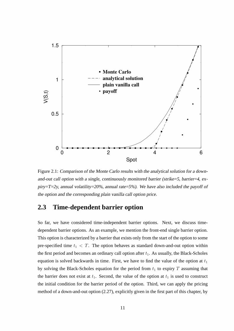
We have performed a Monte Carlo simulation for a down-and-out call option. The under-
lying asset priceSt is simulated in time according to Eq.(2.2). Random numbers are gener-
ated using standard routines from the GNU Scientific Library(GSL) available at [16]. The
number of paths used in the simulation is108. The results of the Monte Carlo simulation
are presented in Fig. 2.1. The result is shown to be in agreement with the analytical solu-
tion in Eq.(2.30). The price of the continuous barrier option converges to the price of an
otherwise identical vanilla call option as the spot price moves away from the barrier.
10
0 2 4 6
Spot
0
0.5
1
1.5V
(S,t)
Monte Carlo
analytical solution
plain vanilla call
payoff
Figure 2.1:Comparison of the Monte Carlo results with the analytical solution for a down-
and-out call option with a single, continuously monitored barrier (strike=5, barrier=4, ex-
piry=T=2y, annual volatility=20%, annual rate=5%). We have also included the payoff of
the option and the corresponding plain vanilla call option price.
2.3 Time-dependent barrier option
So far, we have considered time-independent barrier options. Next, we discuss time-
dependent barrier options. As an example, we mention the front-end single barrier option.
This option is characterized by a barrier that exists only from the start of the option to some
pre-specified timet1 < T . The option behaves as standard down-and-out option within
the first period and becomes an ordinary call option aftert1. As usually, the Black-Scholes
equation is solved backwards in time. First, we have to find the value of the option att1
by solving the Black-Scholes equation for the period fromt1 to expiry T assuming that
the barrier does not exist att1. Second, the value of the option att1 is used to construct
the initial condition for the barrier period of the option. Third, we can apply the pricing
method of a down-and-out option (2.27), explicitly given inthe first part of this chapter, by
11

appropriately replacing the initial conditionu(x, 0) in Eq.(2.24).
To make it more precise, the value of the option att1 is equal to the value of an ordinary
call option if the asset price att1 is above the barrier and zero otherwise
V (S, t1) =
VC(S, t1) S > B
0 S ≤ B
. (2.31)
The value of the option att1 serves now as the initial condition for the barrier option
problem. Next, we apply Eq.(2.27) to find the price of the front-end down-and-out option
V (S, t) = eα1x
∫ ∞
−∞dξ e−α1ξV (Beξ, t1) uG(x, ξ, τ) , (2.32)
whereτ is now given byτ = (t1−t)σ2/2, the initial conditionV (Beξ, t1) by Eq.(2.31) and
the Green’s functionuG(x, ξ, τ) by Eq.(2.26). All other parameters have their usual mean-
ing. The integral expression (2.32) can be rewritten as an integral over the 2-dimensional
multivariate normal distribution function [9], but it mustbe carried out numerically. Note
that this option can be reduced to a combination of a compoundoption, i.e. a call option on
a call option, and a standard digital option (see also the discussion in the first part of section
2.2). The value of the front-end down-and-out option is given by the sum of a compound
option with a strike given by the value of the underlying vanilla call option att1, a standard
digital option with the same strike and their reflected solutions.
Applying the same steps as described above, one can also derive an expression for rear-end
barrier options or other more complicated time-dependent barrier options [9].
In general, this method may also be applied for the discrete barrier problem. Suppose the
barrier is monitored at timeti = i∆t, i = 0, 1, ...m with ∆t = T/m. Then, one first solves
the Black-Scholes equation for the period fromtm = T to tm−1. The result is used as the
initial condition for the next period. The price of a discrete barrier option is obtained after
m steps. The pricing of discrete barrier options will be discussed in more detail in chapter
3.
12

2.4 Down-and-Out call option revisited
In this section, we derive two alternative expressions for the Black-Scholes price of a down-
and-out call option. Basically, the one-dimensional integral (2.27) for the price of a down-
and-out call option is converted into anm-dimensional integral. As indicated at the end of
the previous section, one may solve the continuous barrier option by an iterative procedure.
One starts with solution atτ1 = (tm − tm−1)σ2/2, given by
uG(x, ξ, τ1) = u0(x, ξ, τ1) − u0(−x, ξ, τ1) . (2.33)
Using Eq.(2.31) as the initial condition for the next period, the solution atτ2 is given by
uG(x, ξ, τ2) =
∫ ∞
0
dξ1 (u0(ξ1, ξ, τ1) − u0(−ξ1, ξ, τ1))
× (u0(x, ξ1, τ2 − τ1) − u0(−x, ξ1, τ2 − τ1)) (2.34)
After m steps, i.e. atτm = τ , we have
uG(x, ξ, τm) =
∫ ∞
0
dξ1
∫ ∞
0
dξ2...
∫ ∞
0
dξm−1
×m−1∏
i=0
(u0(ξi+1, ξi, τi+1 − τi) − u0(−ξi+1, ξi, τi+1 − τi)) . (2.35)
Here, we have introduced the notationξm = x, ξ0 = ξ andτm = τ . Alternatively, one may
exploit the semi-group property of the Green’s function of the heat equation, which reads
as
u0(x, ξ, τ) =
∫ ∞
−∞dξ1u0(x, ξ1, τ − τ1)u0(ξ1, ξ, τ1) . (2.36)
Applying this propertym-times to Eq.(2.31) yields the following integral expression for
the Green’s function:
uG(x, ξ, τ) =
∫ ∞
−∞dξ1
∫ ∞
−∞dξ2...
∫ ∞
−∞dξm−1
m−2∏
i=0
u0(ξi+1, ξi, τi+1 − τi)
× (u0(ξm, ξm−1, τm − τm−1) − u0(−ξm, ξm−1, τm − τm−1)) . (2.37)
Clearly, Eq.(2.37) can also be obtained from Eq.(2.35) by a simple change of the region
of integration. The alternative integral expressions (2.35,2.37) have a similar structure as
13
the general solution for discretely monitored down-and-out call option (see section 3.2).
Furthermore, one expects that the discrete barrier option converges to its continuous coun-
terpart in the limit as number of monitoring points goes to infinity. It is therefore convenient
to use these expressions as a starting point to study the asymptotic behaviour of a discrete
barrier option. However, we will not follow these lines. Instead we use the method of
matched asymptotic expansion to study the asymptotic behaviour in chapter 4.
2.5 Double Barriers
Next, we briefly focus our attention on double barrier options. These contracts consist of
an upper barrierB+ and a lower barrierB−. In general, one distinguishes up-and-down out
or knockout and up-and-down in or knockin barrier options. The upper barrier leads to an
additional boundary condition. Thus, the boundary conditions read as
V (S = B−, t) = 0 ; V (S = B+, t) = 0 . (2.38)
Again, we have arrived at a well-known boundary value problem. It can be solved by the
Fourier series method. The price of the continuous double barrier knockout option may be
obtained from
V (S, B−, B+, t) = B−eα1x+α2τuc(x, τ) (2.39)
with uc(x, τ) given by the following Fourier series:
uc(x, τ) =
∞∑
n=1
Cn sin(nπ
ax)
e−n2π2
a2 τ . (2.40)
Here, we have introduceda = ln(B+/B−) andx = ln(S/B−). The Fourier coefficients
Cn are given by
Cn =2
a
∫ a
0
dξu(ξ, 0) sin(nπ
aξ)
. (2.41)
The payoffu(ξ, 0) (2.24) is of course defined only forB− < S < B+ and vanishes outside
this interval. Details of the application of the Fourier method for solving the heat equation
14
can also be found in e.g. [8] and [15]. The integral expression for the Fourier coefficients
Cn (2.41) can be explicitly evaluated for the payoff of a call option. A simple analysis
shows that
Cn = 2(−1)n+1nπe(1−α)a + e(1−α)y
(
nπ cos(
nπa
y)
− (1 − α)a sin(
nπa
y))
n2π2 + (1 − α)2a2
− 2(−1)n+1nπey−αa + e(1−α)y
(
nπ cos(
nπa
y)
+ αa sin(
nπa
y))
n2π2 + α2a2, (2.42)
wherey is defined byy = ln(K/B−). Alternatively, one may solve the boundary value
problem by the Laplace transform method. Then, according toDavydov et al. [2] or Feller
[17], the price of a double barrier option is obtained from (2.27) withuc(x, τ) given by
uc(x, τ) =
∞∑
k=−∞
∫ ∞
−∞dξ u(ξ, 0) (u0(x + 2ka, ξ, τ) − u0(−x + 2ka, ξ, τ)) . (2.43)
Note that (2.40) and (2.43) are different represenations ofthe exact solution. Double barrier
options with discrete monitoring will be studied in more detail in chapter 5.
15
Chapter 3
Pricing of discrete barrier options
As already mentioned in the introduction, most of real financial contracts involving barriers
are based on discrete monitoring events. In the following, we study the pricing of barrier
options with discrete monitoring. First, we discuss the model and the analytical solution of
a down-and-out call option. The analytical solution is compared with the results of a Monte
Carlo simulation. In the following section, we derive an alternative integral expression for
the price of a down-and-out call option. Finally, we presentthe results, as obtained by
Broadie et al. [1, 18] and Kou [19], for the asymptotic behaviour of discrete barrier options
in the limit as the number of monitoring points goes to infinity.
3.1 Model and solution
We start our investigation by setting up the model and obtaining a general solution for a
discrete barrier option. For simplicity, we concentrate onthe down-and-out call option.
Unlike in the continuous case, the asset price is only monitored at instantsti = i∆t =
iT/m, whereT is the expiration date andm − 1 is the number of monitoring points (i =
1, 2, ..., m−1). The option is knocked out, if at one of these instants the asset price is below
the barrier. The barrier levels at these instants are denoted byBi. To simplify the notation,
one defines them-th barrier level as the strike of the option, i.e. we haveBm = K. The
underlying asset price may follow a lognormal random walk. The asset price at then-th
monitoring point under the risk-neutral measure is given by
16
Sn = S0 exp
{
(r − σ2/2)tn + σ√
tn
n∑
i=1
Wi
}
, (3.1)
whereWi ‘s are independent standard normal random variables. The stopping timeτd(Bn, Sn)
is the first time at whichSn hits the barrier levelB
τd(Bn, Sn) = inf {n ≥ 1; Sn ≤ Bn} . (3.2)
Then, the value of this option within the Black-Scholes framework is given by the dis-
counted expectation of the payoff under the risk-neutral measureQ
Vm(S, Bn, t) = EQ[e−r(T−t)max(Sm − Bm, 0) 1τ(Bn,Sn)>m] , (3.3)
whereSm is the asset price at expiry and1τ(Bn,Sn)>m is the indicator function of the cross-
ing of the barrier level. Following Heynen et al. [20] and Tseet al. [11], the value of a
discrete down-and-out call option can be expressed as
Vm(S, t) = SNm(d1(S, Bi, ti), ρ) − Bme−r(tm−t)Nm(d2(S, Bi, ti), ρ) , (3.4)
with Nm(x, ρ) being them-dimensional multivariate normal distribution function defined
by
Nm(x, ρ) =1
((2π)m | ρ |)1/2
∫ x1
−∞...
∫ xm
−∞dx e−
12xT ρ−1x (3.5)
and
d1(S, Bi, ti) =ln(S/Bi) + (r − σ2/2)(ti − t)
σ√
ti − t; d2 = d1 + σ(ti − t)1/2 . (3.6)
The correlation functionρ is given byρij = min((ti − t), (tj − t))/√
(ti − t)(tj − t).
An expression for the inverse matrixρ−1 can be found in Ref.[11]. As can be seen from
Eq.(3.4) and Eq.(3.5), the pricing of a discrete barrier option involves the calculation of an
m-dimensional integral. So far, no simplifications of these integral expressions have been
17
0 1 2 3
Spot
0
1
V(S
,t)
Monte Carlo
analytical solution
plain vanilla call
payoff
continuous barrier call
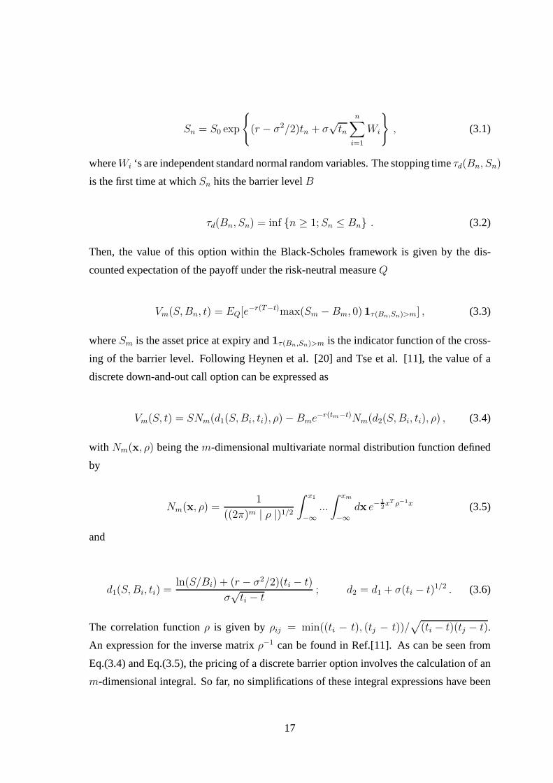
Figure 3.1:Comparison of the Monte Carlo results with the analytical solution for a down-
and-out call option with a single barrier monitored att1 = T/2, whereT is the expiry of the
option (strike=barrier=2, expiry=T=2y, annual volatility=20%, annual rate=5%). We have
also included the payoff of the option, the corresponding plain vanilla call option value and
the corresponding continuous barrier call option value.
derived. Therefore, the integrals must be carried out numerically.
We have performed a Monte Carlo simulation for a down-and-out call option with a single
barrier monitored att1 = T/2. Fig. 3.1 shows a comparison of the Monte Carlo results
with the analytical solution in Eq.(3.4). The results for the analytical solution were obtained
by using a simple adaptive numerical integration procedureprovided by GSL [16]. The
number of paths used in the simulation is108. As in the continuous case the value of the
option is lowered due to the barrier condition.
As mentioned before, the general solution (3.4) for discretely monitored down-and-out
options involves the calculation of anm-dimensional integral overm-dimensional multi-
18
variate normal distribution function and, thus, becomes numerically intractable for a large
number of monitoring points. Therefore, one is interested in alternative numerical pricing
procedures. In the following, I mention various numerical approaches for the pricing of dis-
crete barrier options. Gao et al. [10] have investigated theAdaptive Mesh Model, which is
a trinomial model with adapted time and price steps, i.e. small time and price steps are used
for sections, where high resolution is required and vice versa. A high resolution is required
near the monitoring points and for asset prices close to the barrier. This method permits an
accurate pricing near the barrier and improves the efficiency of the numerical calculation.
Wei [12] proposed a heuristic interpolation formula that isbased on the general solution,
e.g. Eq.(3.4), with the highest number of monitoring pointsthat is analytically tractable on
the one hand and the analytical solution for the continuous case on the other hand. Tse’s et
al. [11] approach is based on the evaluation of the integralsin the exact solution (3.4). They
developed an efficient algorithm for the calculation of the multivariate normal distribution
function for any given accuracy, which is based on the tridiagonal structure of the correla-
tion matrix. Additionally, they incorporated an error bound in the approximation scheme,
which determines the number of evaluation points. Unlike other numerical methods, this
technique works well when the asset price is near the barrier.
3.2 Discrete down-and-out call option revisited
Again, we derive an alternative integral expression for theprice of a discrete down-and-out
call option based on the Black-Scholes equation. Using the standard transformation
Vm(B, S, t) = Beα1x+α2τum(x, t) , (3.7)
the Black-Scholes equation takes the well-known form of theheat equation
∂um
∂τ=
∂2um
∂x2(3.8)
with the initial and boundary condition
um(x, 0) = e−α1xmax(ex − ey, 0) ; um(0, τi) = 0 , (3.9)
19

respectively. As discussed at the end of section 2.4, one maysolve the Black-Scholes
equation iteratively. The solution of the Black-Scholes equation for the period fromτ0 to
τ1 provides the initial condition for the period fromτ1 to τ2 etc. After m steps, we arrive at
the following expression for the Green’s function:
uG(x, ξ, τ) =
∫ ∞
0
dξ1
∫ ∞
0
dξ2...
∫ ∞
0
dξm−1
m−1∏
i=0
u0(ξi+1, ξi, τi+1 − τi) (3.10)
Inserting Eq.(3.10) into Eq.(2.27) yields the price of a discrete down-and-out call option.
3.3 Continuity correction for discrete barrier options
In this section, we present an asymptotic approximation forthe pricing of discrete barrier
options as derived by Broadie et al. [1, 18] and Kou [19]. Theyintroduced a correction
procedure for discrete options, which is based on the observation that in the limit of an in-
finite number of monitoring points the option price of the discrete barrier option converges
to the price of the continuous barrier option. Then, they introduced a continuity correction
for discretely monitored barrier options. The resulting approximation is a simple correction
to the continuous formula. It is based on some general theorems from sequential analysis
[21, 22, 23]. In the following, we present the theorem and sketch its derivation without
going into the details of the proof of the theorem.
According to Broadie et al. [1, 18] and Kou [19], the price of adiscrete barrier option
Vm(S, B, t) can be expressed in terms of its continuous counterpartV (S, B, t) by
Vm(S, B, t) = V(
S, Be±βσ√
T/m, t)
+ o(1/√
m) , (3.11)
with + for an up option and− for a down option and the constant
β = −ζ(1/2)√2π
≈ 0.5826 , (3.12)
with ζ(x) the Riemann zeta function. They interpret this result as a shift of the barrier away
from the spot priceS by a factoreβσ√
T/m. We will use this argument in chapter 4 to derive
the asymptotic solution (3.11) by using the method of matched asymptotic expansions.
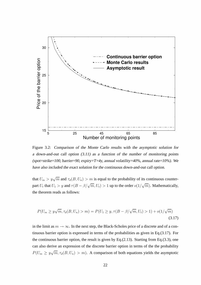
Again, we have performed a Monte Carlo simulation to illustrate the quality of the continu-
ity correction (3.11) as derived by Broadie et al. The results are shown in Fig. 3.2. There,
20

we have made a comparison of the asymptotic solution with theexact solution as a func-
tion of the number of monitoring points. The exact solution is the result of a Monte Carlo
simulation using108 paths. The asymptotic solution converges to the exact solution as the
number of monitoring points increase. Remarkably, the continuity correction is a very good
approximation to the exact solution even for numbers of monitoring points for which the
price of the discrete barrier and the price of the continuousbarrier differ significantly, i.e.
for a number of monitoring points for which the correction contribution to the continuous
barrier option is not a small contribution compared with thecontinuous barrier option. This
is also the reason why most practioners rely on the continuity correction for a wide range of
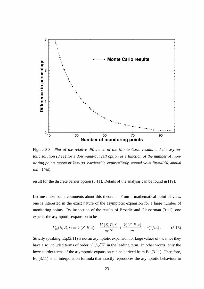
monitoring points instead of using time consuming Monte Carlo simulations. In Fig. 3.3,
we have plotted the relative difference of the exact solution and the asymptotic solution
for the numerical results shown in Fig 3.2. For the parameterchosen in this example, the
difference between the continuity correction and the exactsolution is less than0.1% for 90
monitoring points.
Broadie et al. [1, 18] and Kou [19] have presented various proofs of equation (3.11). The
shortest and most transparent proof has been given by Kou [19]. In the following, we
outline the main steps of this proof. Kou‘s approach is basedon a theorem by Siegmund
and Yuh [23] that was later extended by Kou [19]. The theorem connects the first exit time
τd(B, Un) = inf{n ≥ 1 : Un ≤ B√
m} (3.13)
of a discrete random walk
Un =n∑
i=1
(Wi + µ/√
m) , (3.14)
whereWi’s are independent standard normal random variables, and the first exit time
τ(B, Ut) = inf{t ≥ 0 : Ut ≤ B} (3.15)
of a continuous Brownian motion
Ut = Wt + µt , (3.16)
whereµ is the drift of the process. Here,Un describes a random walk with a small drift
µ/√
m asm → ∞. The theorem states that the probability of a discrete random walk Un
21
5 25 45 65 85
Number of monitoring points
15
20
25
30
Price
of
the
ba
rrie
r o
ptio
n
Continuous barrier option
Monte Carlo results
Asymptotic result
Figure 3.2: Comparison of the Monte Carlo results with the asymptotic solution for
a down-and-out call option (3.11) as a function of the numberof monitoring points
(spot=strike=100, barrier=90, expiry=T=4y, annual volatility=40%, annual rate=10%). We
have also included the exact solution for the continuous down-and-out call option.
thatUm > y√
m andτd(B, Un) > m is equal to the probability of its continuous counter-
partUt thatU1 > y andτ(B − β/√
m, Ut) > 1 up to the ordero(1/√
m). Mathematically,
the theorem reads as follows:
P (Um ≥ y√
m, τd(B, Un) > m) = P (U1 ≥ y, τ(B − β/√
m, Ut) > 1) + o(1/√
m)
(3.17)
in the limit asm → ∞. In the next step, the Black-Scholes price of a discrete and of a con-
tinuous barrier option is expressed in terms of the probabilities as given in Eq.(3.17). For
the continuous barrier option, the result is given by Eq.(2.13). Starting from Eq.(3.3), one
can also derive an expression of the discrete barrier optionin terms of the the probability
P (Um ≥ y√
m, τd(B, Un) > m). A comparison of both equations yields the asymptotic
22
10 30 50 70 90
Number of monitoring points
0
1
2
3D
iffe
ren
ce in
perc
en
tag
e Monte Carlo results
Figure 3.3: Plot of the relative difference of the Monte Carlo results and the asymp-
totic solution (3.11) for a down-and-out call option as a function of the number of mon-
itoring points (spot=strike=100, barrier=90, expiry=T=4y, annual volatility=40%, annual
rate=10%).
result for the discrete barrier option (3.11). Details of the analysis can be found in [19].
Let me make some comments about this theorem. From a mathematical point of view,
one is interested in the exact nature of the asymptotic expansion for a large number of
monitoring points. By inspection of the results of Broadie and Glasserman (3.11), one
expects the asymptotic expansion to be
Vm(S, B, t) = V (S, B, t) +V1(S, B, t)
m1/2+
V2(S, B, t)
m+ o(1/m) . (3.18)
Strictly speaking, Eq.(3.11) is not an asymptotic expansion for large values ofm, since they
have also included terms of ordero(1/√
m) in the leading term. In other words, only the
lowest order terms of the asymptotic expansion can be derived from Eq.(3.11). Therefore,
Eq.(3.11) is an interpolation formula that exactly reproduces the asymptotic behaviour to
23

the lowest order in the expansion parameter1/√
m.
24

Chapter 4
Asymptotic expansion for single barrier
options
In this chapter, we perform an asymptotic expansion of the discrete down-and-out call op-
tion in the limit of a high number of monitoring events. First, we study the asymptotic
result for the discrete barrier option as obtained by Broadie et al. (3.11). We calculate its
value at the boundaryS = B, which gives an effective boundary condition. By reversing
of the argument, we show that the knowledge of the effective boundary condition at the
original boundaryS = B yields the asymptotic result for the discrete barrier option. Sec-
ond, we introduce the method of matched asymptotic expansions. In particular, we present
Van Dyke’s matching principle. Finally, we apply the methodof matched asymptotic ex-
pansions to calculate the effective boundary condition atS = B. The result can then be
used to calculate the value of the discrete barrier option inthe limit of a high number of
monitoring points.
4.1 General remarks
In this section, we analyse the asymptotic result for the discrete down-and-out option as
derived by Broadie et al. In particular, we pay attention to the argument by Broadie et al.
that the price of the continuous barrier option may serve as an approximation to the price
of a discrete barrier option, if one shifts the barrier away from the spot priceS by a factor
eβσ√
T/m. We will show that this leads to an effective non-vanishing boundary condition
25

at the boundary of the continuous barrier option. Solving the Black-Scholes equation for
S > B with the effective boundary condition gives the approximation to the price of the
discrete barrier option. In other words, the knowledge of the effective boundary condition
at S = B provides a simple way of the calculation of price of a discrete barrier option.
Clearly, the effective boundary condition atS = B will only be determined in the limit
of a high number of monitoring points. The effective boundary condition atS = B in the
asymptotic limit can be determined by the method of matched asymptotic expansions using
Van Dyke’s matching principle. This will be discussed in thefollowing sections.
For the following investigations, it is convenient to introduce the small parameter
ǫ = σ√
T/m . (4.1)
The starting point of our investigation is the asymptotic result for the discrete barrier op-
tion Vm(S, B, t) given in Eq.(3.11). By inspection of this equation, one observes that
the value of the discrete down-and-out option is approximately the value of the continu-
ous down-and-out option with the barrier shifted toBe−βσ√
T/m. In terms of the variable
x = ln(S/B) as defined in Eq.(2.21) the boundary is shifted from 0 to−βǫ. Expanding
Eq.(3.11) to first order in the small parameterǫ yields
Vm(S, B, t) = V (S, B, t) + ǫ∂V (S, Be−βǫ, t)
∂ǫ
∣
∣
∣
ǫ=0+ ... , (4.2)
whereV (S, B, t) is the solution of the continuous down-and-out call option.Next, we
compute the value of the discrete option at the boundaryS = B and in the asymptotic limit
m → ∞. The result is readily found to be
Vm (B, B, t) = βǫB∂V (S, B, t)
∂S
∣
∣
∣
S=B+ o(ǫ) . (4.3)
Alternatively, one may express the boundary condition in terms of the transformed vari-
ablex and functionuc(x, τ) that satisfies the heat equation with a homogeneous boundary
condition atx = 0 (2.23-2.24). In terms ofuc(x, τ), the boundary condition (4.3) can be
rewritten as
Vm (B, B, t) = βǫBeα2τγ(τ) + o(ǫ) (4.4)
26

with γ(τ) given by
γ(τ) =∂uc(x, τ)
∂x
∣
∣
∣
x=0. (4.5)
Thus, we have derived the effective boundary condition atS = B for Vm(S, B, t) or equiv-
alently forum(x, τ) (3.7) atx = 0. In other words, the value of the discrete barrier option
in the asymptotic limit may be obtained from solving the original initial boundary value
problem for the continuous barrier (2.23-2.24) with the effective boundary condition given
by u(0, τ) = βǫγ(τ) instead ofu(0, τ) = 0.
One may look at this problem from a different perspective by reversing the argument. As-
sume that we know the boundary condition atx = 0 for the discrete barrier option and it is
given by
um(0, τ) = βǫγ(τ) . (4.6)
Then, we solve the corresponding heat equation
∂um
∂τ=
∂2um
∂x2(4.7)
in the quarter planex > 0 andτ > 0 with the initial and boundary conditions
um(x, 0) = e−α1xmax(ex − ey, 0) ; um(0, τ) = βǫγ(τ) , (4.8)
respectively. The general solution to this problem can be written as
um(x, τ) = uc(x, τ) + u1(x, τ) , (4.9)
whereuc(x, τ) is the solution of the continuous barrier as defined in Eq.(2.27), i.e. it
satisfies the homogeneous boundary condition. Therefore,u1(x, t) is the solution of the
heat equation that satisfies the boundary condition (4.8) and vanishes atτ = 0. This
problem is solved by Duhamel‘s formula
u1(x, τ) = βǫ
∫ τ
0
ds γ(τ − s)G(x, s) (4.10)
with
G(x, τ) =x
(4π)1/2τ 3/2e−
x2
4τ . (4.11)
27
The s-integration in (4.10) can be carried out exactly. The detailed evaluation of this in-
tegral is given in appendix A. Performing the integration, one arrives at the following ex-
pression foru1(x, t)
u1(x, τ) = βǫ1
(4π)1/2τ 3/2
∫ ∞
−∞dξu(ξ, 0)(x + ξ)e−
(x+ξ)2
4τ . (4.12)
Finally, we use the standard transformation from the Black-Scholes equation to the heat
equation (2.21) to derive the asymptotic result for the discrete barrier option as given in
(4.2). Thus, we have shown that solving the Black-Scholes equation subject to the effective
boundary condition (4.4) atS = B leads to the asymptotic result for the price of the discrete
barrier option as obtained by Broadie et al. [1].
Again, one may look at this problem from a different perspective. We are looking for a
solution to the boundary problem (4.7-4.8) of the form (4.9). We know thatuc(x, τ) can
be written as the sum of the vanilla call optionu+c (x, τ) and its image solutionu−
c (x, τ)
according to Eqs.(2.27-2.29). Thus, we have
uc(x, τ) = u+c (x, τ) + u−
c (x, τ) . (4.13)
Additionally, we know that∂u−c (x, τ)/∂x satisfies the heat equation (4.7) and that its value
at τ = 0 for x > 0 is zero, i.e.u−c (x, 0) = 0. To study the boundary condition, we observe
that
∂uc(x, τ)
∂x
∣
∣
∣
x=0=
∂u+c (x, τ)
∂x
∣
∣
∣
x=0+
∂u−c (x, τ)
∂x
∣
∣
∣
x=0= 2
∂u−c (x, τ)
∂x
∣
∣
∣
x=0(4.14)
since by reflectionu+c (x, τ) = −u−
c (−x, τ). Thus, the following expression foru1(x, τ) is
a solution of the heat equation and satisfies the initial and boundary condition:
u1(x, τ) = 2βǫ∂u−
c (x, τ)
∂x. (4.15)
Inserting Eq.(2.29) into (4.15) yields the integral expression (4.12). Then, we can apply the
same argument as discussed above to show that this equation leads to the asymptotic result
for the price of the discrete barrier option as obtained by Broadie et al. [1].
We are left with the determination of the effective boundarycondition at the barrier. This
will be the subject of the following sections. Using the method of matched asymptotic
28
expansions and Van Dyke’s matching principle, we work out the value of the discrete barrier
option at the boundary up to the ordero(ǫ). The result is used to calculate the asymptotic
behaviour for the discrete barrier option for all values ofx as outlined in this section. In the
following section, we briefly explain the method of matched asymptotic expansions and
Van Dyke’s matching principle that are used to derive asymptotic expressions for solving
partial differential equations.
4.2 Van Dyke’s matching principle
In this section, we briefly present the method of matched asymptotic expansions. The
method of matched asymptotic expansions is often used in connection with problems for
which the exact solution changes rapidly from one domain to another. In other words,
the solution cannot be found as an expansion in terms of a single scale, but of two or
more scales each valid in a separate part of the domain. Typical examples of these kind
of problems are transition layer problems such as boundary layer, initial layer and internal
layer problems. As we will show in the next section, the discrete barrier option is also an
example of a layer problem. Here, the solution changes rapidly when the asset price hits the
barrier. In the following, we only discuss the general idea of Van Dyke’s matching method.
In doing so, we essentially follow the lines of Campell [24].An introduction to the method
of matched asymptotic expansions can also be found in [25, 26, 27, 28, 29].
Assume that a functionyo(x, ǫ) is the solution of a differential equation in one part of
the domain, generally referred to as the outer solution. Thesolution in the other part of
the domain, generally referred to as the inner solution, maybe given byyi(ξ, ǫ). Hereξ
is the inner variable that is obtained from the outer variable x by rescaling according to
ξ = x/α(ǫ) with an appropriately chosen functionα(ǫ). We look for an approximation
to the exact solution in the limit as the parameterǫ goes to zero. In order to create an
approximation to the exact solution that is valid over the entire domain, we need to match
the inner to the outer solution. Van Dyke’s method provides away to fit these solutions
together. In the following, we present the three hypotheseson which Van Dyke’s matching
principle are based.
First, we introduce then-term inner expansion operatorIn and them-term outer expansion
operatorOm. When acting on any functiony, these operators are defined as follows:
29
In = express the function in terms of the inner variableξ and then expand in powers ofǫ,
truncating all but the firstn terms.
Om = express the function in terms of the outer variablex and then expand in powers ofǫ,
truncating all but the firstm terms.
Van Dyke’s hypotheses can now be expressed in terms of the inner and outer expansion
operators. The first Van Dyke’s hypothesis concerns the exact solutionye and reads as
OmInye = InOmye . (4.16)
This hypothesis basically states that the inner and outer expansion operators are commuta-
tive when applied to the exact solution. In other words, the outcome of the application of
both operators on the exact solution is independent of the order of application. The next
two hypotheses concern the inner and the outer expansion andare given by the following
equations
Inye = yi , (4.17)
Omye = yo . (4.18)
These hypotheses relate the inner expansion of the exact solution with them-term inner
solution and the outer expansion of the exact solution with then-term outer solution. How-
ever, the exact solution is in general not available. If the exact solution is known, the search
for an approximation to the exact solution is unnecessary. The use of Van Dyke’s hypothe-
ses becomes clear, when one relates the inner expansion of the outer solution to the outer
expansion of the inner solution. This can be achieved by substituting (4.17) and (4.18) in
(4.16). We get
Inyo = Omyi . (4.19)
Thus, we have found a way for matching the outer solution withthe inner solution. Eq.(4.19)
states in words that
Then-term outer expansion of them-term inner solution equals them-term inner expansion
of then-term outer solution
30
The remaining task is to find a composite solutionyc that is valid in the entire domain. This
can be accomplished by the equation
yc = yi + yo − Omyi = yi + yo − Inyo . (4.20)
Unfortunately, Van Dyke’s matching rule does not always work. In particular, the method
may fail in problems for which the respective validity domains of the outer and inner solu-
tion do not overlap. Then, one can introduce an intermediateexpansion that connects the
different domains. Details on this subject can be found in [25, 26, 27, 28, 29].
In the next section, we apply Van Dyke’s matching method to compute an approximation to
the discrete down-and-out option for which the time betweenmonitoring events becomes
small.
4.3 Matched asymptotic expansions
In this section, we apply the method of matched asymptotic expansions to derive the effec-
tive boundary condition at the barrier. This condition is used to calculate the asymptotic
result for the discrete down-and-out option as outlined in section 3.3.
First, let us discuss the behaviour of the solution above thebarrier, i.e. forx > 0, in the
limit as the number of monitoring pointsm goes to infinity. This domain will be referred to
as the outer region. Obviously, the outer solution converges to the price of the continuous
barrier option asm → ∞. Relative to the reset timescale, this is a slowly varying function.
For largem, one expects a correction term to the continuous barrier option that vanishes
as the number of monitoring points go to infinity. In other words, the detailed nature of
the boundary condition atx < 0 leads to a small correction contribution to the price of
the continuous barrier option for large m. Thus, we look for an outer solution of the initial
boundary value problem (3.8,3.9) of the form
uo2(x, τ) = uc(x, τ) + δ(ǫ)u1(x, τ) , (4.21)
whereuc(x, τ) is the solution of the heat equation for the continuous barrier option. The
functionδ(ǫ) of the small parameterǫ = σ√
T/m as defined in (4.1) andu1(x, τ) must be
31
determined.
The behaviour of the solution below the barrier, i.e. forx < 0, is different. This domain
will be referred to as the inner region. The slow scale is not appropriate in the inner domain.
As a consequence of the boundary condition, the solution is approximately time periodic
in the inner domain. Therefore, it is convenient to introduce faster variables in the inner
domain given by
τ = τi + ǫ2s; x = ǫξ , (4.22)
whereτi is an arbitrary reset. The outer solution satisfies the boundary condition atx → ∞.
However, in general, it does not satisfy the boundary condition at x < 0. Contrary, the
inner solution satisfies the boundary condition forx < 0 and does not satisfy the boundary
condition atx → ∞. In order to find a solution valid in the entire domain, we haveto
match the inner and the outer solution in a region nearx = 0. This can be achieved by
applying Van Dyke’s matching principle as discussed in the previous section.
First, we express the outer solution (4.21) in terms of the inner variables and expand to first
order in the small parameterǫ. We know thatuc(x, τ) ∼ γ(τ)x + o(x) for x → 0. Next,
we study the one-term inner expansion of the one-term outer solution. We obtain
I1uo1(ξ, τ) = ǫγ(τ)ξ . (4.23)
As will be shown below, this equation may be used to determinethe functionδ(ǫ). Now,
we compute the one-term inner expansion of the two-term outer solution. We express the
outer solution (4.21) in terms of the inner variables and expand to first order inǫ. We find
that
I1 uo2(ξ, τ) = ǫγ(τ)ξ + δ(ǫ)u1(0, τ) . (4.24)
Next, we solve a canonical inner problem. The solution to theinner problem is time-
periodic to the lowest order of accuracy in the small parameter ǫ. We will also change
the independent variables from(x, τ) to (ξ, s) according to Eq.(4.22). The heat equation
equation for the inner solution becomes
32
∂uim
∂s=
∂2uim
∂ξ2, (4.25)
with the initial condition
uim(ξ, 0) = 0, ξ < 0 ; ui
m(ξ, 0) = F (ξ), ξ > 0, (4.26)
and the periodicity condition
uim(ξ, 0) = ui
m(ξ, 1) = F (ξ) , (4.27)
respectively. A standard way for solving this type of partial differential equation is the
method of Green’s functions as discussed in the previous sections. The general solution
is found by applying the iterative procedure described in sections 2.4 and 3.2. Imposing
periodicity on the solution leads to the following integralequation:
F (ξ) =
∫ ∞
0
dyF (y)u0(ξ, y, 1) , (4.28)
whereu0(ξ, y, 1) is the heat kernel as defined in Eq.(2.25). This integral equation has been
extensively studied by Spitzer [30, 31] in connection with problems in probability theory.
Spitzer has shown that there is a unique non-decreasing positive solution to the integral
equation. The general solution to the integral equation (4.28) is obtained by the Laplace
transform. The Laplace transform ofF (ξ) is given by
∫ ∞
0
e−λξF (ξ)dξ = exp
{
− 1
2π
∫ ∞
−∞
λ
λ2 + y2ln[
1 − e−y2/2]
dy
}
− 1 . (4.29)
Furthermore, Spitzer has shown that the asymptotic behaviour of F (ξ) at large values ofξ
reads as
limξ→∞
F (ξ) =√
2
(
ξ +1
2π
∫ ∞
−∞y−2 ln
[
(y2/2)(1 − e−y2/2)−1]
dy
)
. (4.30)
Chernoff [32] has calculated the approximate value0.5824 for the constant in (4.30). Chang
et al. [33] have shown that the constant is given by−ζ(1/2)/√
2π = 0.5826. Thus, the
asymptotic behaviour ofF (ξ) can be written as
33

limξ→∞
F (ξ) =√
2(
ξ − ζ(1/2)/√
2π)
. (4.31)
Next, we apply the arguments of Van Dyke’s matching principle. We start with the one-
term inner solution. We have found a solution to a canonical inner problem (4.25-4.27)
given byF (ξ). The inner solution is modulated by the time-dependent function γ(τ) from
the outer solution. Thus, the one-term inner solution readsas
uim(ξ, τ) = α(ǫ)γ(τ)F (ξ) . (4.32)
Now, to determineα(ǫ), we compute the one-term outer expansion of the one-term inner
solution. Therefore, we express the inner solution (4.32) in terms of the outer variables
and expand in powers ofǫ, keeping the first term only. The behaviour ofF (x/ǫ) for small
values ofǫ, i.e. ξ = x/ǫ → ∞, is given by (4.31). Obviously, only the first term in (4.31)
contributes to the one-term outer expansion of the one-terminner solution. We find that
O1 ui1(x, τ) =
√2α(ǫ) γ(τ) ξ =
√2α(ǫ) γ(τ)
x
ǫ. (4.33)
This enables us to determineα(ǫ) by matching the one-term inner expansion of the one-
term outer solution (4.23) with the one-term outer expansion of the one-term inner solution
(4.33). Thenα(ǫ) becomes
α(ǫ) = ǫ/√
2 . (4.34)
Now, we apply van Dyke’s matching argument for the two-term outer expansion and the
one-term inner expansion. The one-term inner expansion of the two-term outer solution
is given in Eq.(4.24). Using (4.34), the two-term outer expansion of the one-term inner
solution is given by
O2 ui1(ξ, τ) = ǫγ(τ)
(
ξ − ζ(1/2)/√
2π)
. (4.35)
Since by matching argumentsO2ui1 = I1u
o2 we can see thatδ(ǫ)u1(0, τ) takes the form
δ(ǫ)u1(0, τ) = −ǫγ(τ)ζ(1/2)/√
2π (4.36)
34

Finally, we compute the value of the outer solution at the boundaryx = 0. Inserting (4.36)
in (4.21) and settingx = 0 yields
uo2(0, τ) = −ǫγ(τ)ζ(1/2)/
√2π . (4.37)
Thus, we have derived the effective boundary condition seenby the outer problem. This
result exactly coincides with the boundary condition as assumed in Eq.(4.6). Following the
argument as outlined at the end of section 4.1, the price of the discrete down-and-out call
option in the limit of a high number of monitoring points is approximately given by
Vm(S, B, t) = V (S, B, t) + ǫ∂V (S, Be−βǫ, t)
∂ǫ
∣
∣
∣
ǫ=0+ o(ǫ) . (4.38)
Finally, we follow the ideas of Broadie et al. [1] and proposean interpolation formula that
exactly reproduces the asymptotic behaviour to the lowest order in the expansion parameter
1/√
m given by
Vm(S, B, t) = V(
S, Be−βσ√
T/m, t)
+ o(1/√
m) . (4.39)
This result coincides with the continuity correction (3.11) as derived by Broadie et al.
[1]. Note that this derivation can aso be used to get an asymptotic expression for the
other types of barrier options such as discrete up-and-out or discrete up-and-in options.
The discrete down-and-in option is obtained by replacing the first derivative of the price
of the continuous down-and-out option with respect tox in (4.23) by the first derivative
of the price of the continuous down-and-in option with respect to x and using the same
argumentation as discussed in this section. For discrete up-and-out and discrete up-and-in
option, one additionally has to replaceǫγ(τ)ξ by −ǫγ(τ)ξ in (4.23). This leads to a shift
of the barrier fromB to Be+βǫ instead ofBe−βǫ.
35

Chapter 5
Asymptotic expansion for double barrier
options
In this chapter, we study discrete double barrier options. We apply the method of matched
asymptotic expansions to derive an asymptotic expression for discrete double barrier op-
tions. In doing so, we essentially follow the lines as presented for single barrier options in
chapter 4.
5.1 Matched asymptotic expansions
Double barrier options with continuous monitoring have been discussed in section 2.5.
Now we focus on double barrier options with discrete monitoring. As for single barrier
options, the price of discrete double barrier options can beexpressed by anm-dimensional
integral using the Green’s function method as discussed in section 2.4. Since the compu-
tational effort increases rapidly at largem, one is interested in an asymptotic result for the
price of discrete double barrier options that provides a good approximation at largem. In
other words, we want to study the asymptotic behaviour of discrete double barrier options
in the limit as the number of monitoring points goes to infinity.
The asymptotic behaviour of discrete single barrier options has been the topic of chapter 4.
The methods applied to discrete single barrier options can also be used for discrete double
barrier options. The basic idea is to work out the efficient boundary condition atx = 0
andx = a by using the method of matched asymptotic expansions. The result is used to
36

formulate a boundary value problem with time-dependent boundary conditions, which can
then be solved by standard methods such as the Laplace transform.
Following the same ideas as outlined in section 4.3, we look for an outer solution of the
original boundary value problem. Suppose the two-term outer solution of a discrete double
barrier knockout option is given by
uo2(x, τ) = uc(x, τ) + δ(ǫ)u1(x, τ) , (5.1)
whereuc(x, τ) is the solution for the continuous double barrier option as given by (2.40).
We want to determine the functionsδ(ǫ) andu1(x, τ) by applying the method of matched
asymptotic expansions. First, we observe that the behaviour of the solution is different in
the domainsx ≤ 0 andx ≥ a on the one hand and in the domain0 < x < a on the other
hand. In the domainx ≤ 0 andx ≥ a, the solution is approximately time-periodic due
to the boundary condition. In the domain0 < x < a, the solution is slowly varying and
converges to the price of the continuous double barrier option asm → ∞. In contrast to
single barrier options, there are two regionsx ≈ 0 andx ≈ a for double barrier options
in which the solution rapidly changes. However, to lowest order, the detailed nature of
the boundary condition atx = a does not influence the solution atx = 0 and vice versa.
In other words, if we work out the outer solution atx ≈ 0, we assume that the boundary
condition atx = a is zero, i.e. we assume that the boundary condition is that ofthe
continuous double barrier option, and vice versa.
Next, we apply the same arguments as for single barrier options. We expand the solution
for the continuous double barrier option nearx ≈ 0. The first derivative ofuc(x, τ) with
respect tox at x = 0 serves to modulate the solution in the domainx ≤ 0. Then, we
follow exactly the same steps as outlined in section 4.3 to compute the effective boundary
condition atx = 0. Here, we only present the result without going into the details of the
calculation. The effective boundary condition atx = 0 is given by
uo2(0, τ) = βǫγ(0, τ) , (5.2)
whereγ(x, τ) can be expressed in terms of the solution of the continuous double barrier
option as
37

γ(x, τ) =∂uc(x
′, τ)
∂x′
∣
∣
∣
x′=x. (5.3)
Inserting (2.40) foruc(x, τ), one finds
γ(0, τ) =∞∑
n=1
Cn
(nπ
a
)
e−n2π2
a2 τ . (5.4)
The effective boundary condition atx = a is obtained similarly. The first derivative of
uc(x, τ) with respect tox at x = a determines the solution in the domainx ≥ a. Again,
we can apply the same steps as outlined in section 4.3 to compute the effective boundary
condition atx = a. Alternatively, one may consider symmetry arguments. If weshift the
boundary froma to 0 and reflect the solution, i.e. we introduceu1(−x, τ), we have derived
exactly the same problem that has led to the effective boundary condition (5.2) atx = 0
in terms of the original variable. The transformation can beachieved by introducing the
new variablex′ = −(x − a). Both methods give the following expression for the effective
boundary condition atx = a:
uo2(a, τ) = −βǫγ(a, τ) , (5.5)
with γ(a, τ) defined by
γ(a, τ) =
∞∑
n=1
(−1)nCn
(nπ
a
)
e−n2π2
a2 τ . (5.6)
So far, we have derived the effective boundary conditions for the outer problem. In the next
step, we use this result to solve the following initial boundary value problem:
∂um
∂τ=
∂2um
∂x2(5.7)
with the initial condition
um(x, 0) = e−α1x max (ex − ey, 0) (5.8)
and the boundary conditions
38
um(0, τ) = βǫγ(0, τ) ; um(a, τ) = −βǫγ(a, τ) . (5.9)
The continuous double barrier optionuc(x, τ) satisfies the heat equation with initial condi-
tion (5.8) and vanishing boundary condition. The solution to the boundary value problem
can written as
um(x, τ) = uc(x, τ) + βǫu1(x, τ) , (5.10)
whereu1(x, τ) satisfies the heat equation with vanishing initial condition and with time-
dependent boundary conditions (5.9). The general solutionto this standard problem is
obtained by the Laplace transform. Details of the derivation can be found in [34]. We
obtain
u1(x, τ) =2
a
∞∑
k=1
∫ τ
0
ds
{
γ(0, s) sin
(
kπ
ax
)
− γ(a, s) sin
(
kπ
a(a − x)
)}
×(
kπ
a
)
e−k2π2
a2 (τ−s) . (5.11)
The remainings-integration in this expression can be immediately carriedout. The result
reads as follows:
u1(x, τ) =2
a
∞∑
k=1
{
Ak sin
(
kπ
ax
)
− Bk sin
(
kπ
a(a − x)
)}
e−k2π2
a2 τ (5.12)
with the coefficientsAk andBk given by
Ak = Ckπ2k2
a2τ +
∞∑
n=1n6=k
Cnnk
k2 − n2
(
e−π2
a2 (n2−k2)τ − 1
)
(5.13)
and
Bk = (−1)kCkπ2k2
a2τ +
∞∑
n=1n6=k
(−1)nCnnk
k2 − n2
(
e−π2
a2 (n2−k2)τ − 1
)
, (5.14)
39
respectively. The coefficientsCn are given in (2.42) for the payoff of a call option. Alter-
natively, one may insert the payoff of a put option in (2.41) to get the asymptotic result for
a double knockout put option.
0 50 100
Number of monitoring points
0.46
0.56
0.66
0.76
Price o
f th
e b
arr
ier
option
Continuous barrier option
Monte Carlo results
Asymptotic result
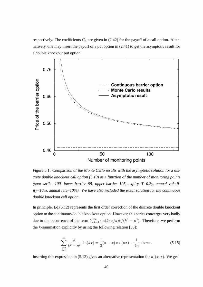
Figure 5.1:Comparison of the Monte Carlo results with the asymptotic solution for a dis-
crete double knockout call option (5.19) as a function of thenumber of monitoring points
(spot=strike=100, lower barrier=95, upper barrier=105, expiry=T=0.2y, annual volatil-
ity=10%, annual rate=10%). We have also included the exact solution for the continuous
double knockout call option.
In principle, Eq.(5.12) represents the first order correction of the discrete double knockout
option to the continuous double knockout option. However, this series converges very badly
due to the occurrence of the term∑∞
k=1 sin(kπx/a)k/(k2 − n2). Therefore, we perform
thek-summation explicitly by using the following relation [35]:
∞∑
k=1k 6=n
k
k2 − n2sin(kx) =
1
2(π − x) cos(nx) − 1
4nsin nx . (5.15)
Inserting this expression in (5.12) gives an alternative representation foru1(x, τ). We get
40
u1(x, τ) =2
a
∞∑
k=1
{
ak sin
(
kπ
ax
)
+ bk cos
(
kπ
ax
)}
e−k2π2
a2 τ (5.16)
with the coefficientsak andbk given by
ak = 2Ckπ2k2
a2τ − Ck
2−
∞∑
n=1n6=k
Cnnk
k2 − n2
(
1 + (−1)n+k)
(5.17)
and
bk = Ckkπ
2a(a − 2x) , (5.18)
respectively.
Finally, we summarize the results. The asymptotic result for the discrete double barrier
knockout option to lowest order can be written as
Vm(S, B−, B+, t) = B−eα1x+α2τ (uc(x, τ) + βǫu1(x, τ) + o(1/√
m)) , (5.19)
whereu1(x, τ) is given by (5.12) or (5.16). In order to compare the asymptotic result (5.19)
with the exact solution, we have performed a Monte Carlo simulation for a discrete double
knockout call option. Fig. 5.1 shows a comparison of the Monte Carlo results with the
asymptotic result in Eq.(5.19). The number of paths used in the simulation is5 × 107.
The simulation shows that Eq.(5.19) adequately describes the asymptotic behaviour of a
discrete double knockout call option. Note that this methodcan also be applied to derive
an asymptotic result for the discrete double barrier knockin option.
41

Chapter 6
Conclusion and Outlook
In this thesis, we have studied the pricing of discrete barrier options using analytical meth-
ods and numerical simulations. In particular, we have introduced the method of matched
asymptotic expansions to study the asymptotic behaviour ofdiscrete barrier options. In a
first approach, we have used this method to perform an asymptotic expansion for discrete
single barrier options. As a result of our analysis, we have derived the first order correc-
tion of the price of a discrete single barrier option to the price of the continuous single
barrier option (4.38). This result coincides with the continuity correction (3.11) as derived
by Broadie et al. [1] within a probability approach. In the next step, we have applied this
method to discrete double barrier options to derive an asymptotic result for largem. Again,
we have derived the first order correction of the price of a discrete double barrier option to
the price of the continuous double barrier option (5.19).
A subject of future investigation might be the extension of the method outlined in this the-
sis to incorporate a local volatility surface. This is completely inaccessible by probability
methods. The general method may also be extended to discretelookback or hindsight op-
tions as discussed in [18]. It may also serve as a starting point to study more exotic barrier
options with discrete monitoring such as corridor options or barrier options with curved
barriers. In principle, one can also proceed to higher orderterms in the asymptotic expan-
sion. The periodic structure of the inner solution will be modulated by a time-dependent
function from the outer solution for higher order contributions.
42
Appendix A
Useful integral
In this appendix, we present the calculation of an integral used in section 4.1. The integral
reads as follows
∫ 1
0
dx1
x3/2 (1 − x)3/2e−
ax− b
1−x , (A.1)
with a>0 and b>0. After the substitutionx = 1/(x′ + 1), this equation may be rewritten as
=
∫ ∞
0
dxx + 1
x3/2e−ax− b
x e(−a−b) , (A.2)
where we have dropped the prime. Now, we may perform the integration (see reference
[35], page (344), equation (3)) to obtain the following result
=
(
π
ae−2
√ab − π
a
∂
∂be−2
√ab
)
e(−a−b) . (A.3)
Simple algebra yields the final expression for the integral.Thus, we arrive at the following
expression for the integral
∫ 1
0
dx1
x3/2 (1 − x)3/2e−
ax− b
1−x =√
π
(√a +
√b√
ab
)
e−(√
a+√
b)2
. (A.4)
This integral expression is used in section 4.2 to find an approximate result for the discrete
barrier option for a high number of monitoring points.
43

Bibliography
[1] M. Broadie, P. Glasserman, and S. Kou, Mathematical Finance7, 325 (1997).
[2] D. Davydov, and V. Linetsky,Structuring, Pricing and Hedging Double-Barrier Step
Options, working paper.
[3] T.H.F. Cheuk, and T.C.F. Vorst, Risk9, 64 (1996).
[4] R.C. Merton, Bell J. Econ. Manag. Sci.4, 141 (1973).
[5] N. Kunitomo, and M. Ikeda, Mathematical Finance2, 272 (1992).
[6] H. Geman, and M. Yor, Mathematical Finance6, 365 (1996).
[7] A. Pelsser, Finance and Stochastics4, 95 (2000).
[8] C.H. Hui, Applied Financial Economics6, 343 (1996).
[9] C.H. Hui, The Journal of Futures Markets17, 667 (1997).
[10] D.H. Ahn, S. Figlewski, and B. Gao,Pricing Discrete Barrier Options with an Adap-
tive Mesh Model, working paper.
[11] W.M. Tse, L.K. Li, and K.W. Ng, Management Science47, 383 (2001).
[12] J.Z. Wei, Journal of Derivatives51, 51 (1998).
[13] M. Baxter, A. Rennie,Financial Calculus, (Cambridge, Cambridge University Press,
1996).
[14] T.R. Bielecki, M. Rutkowski,Credit Risk: Modelling, Valuation and Hedging, (Hei-
delberg, Springer-Verlag Berlin Heidelberg, 2002).
44

[15] A. Sommerfeld, Partielle Differentialgleichungen in der Physik(Verlag Harri
Deutsch-Thun, Frankfurt/M, 1992).
[16] GNU Scientific Library is available atwww.gnu.org/software/gsl/gsl.html
[17] W. Feller,An Introduction to Probability Theory and Its Application Iand II (Wiley,
New York, 1966).
[18] M. Broadie, P. Glasserman, and S. Kou, Finance and Stochastics3, 55 (1999).
[19] S.G. Kou, available at www.columbia.edu/∼sk75/stat/stat.html or
www.columbia.edu/∼sk75/sinica.pdf. To appear in Statistica Sinica (2003).
[20] R.C. Heynen, and H.M. Kat, Journal of Financial Engineering 5, 199 (1996).
[21] D. Siegmund, Adv. Appl. Prob.11, 701 (1979).
[22] Y.-S. Yuh, Adv. Appl. Prob.14, 566 (1982).
[23] D. Siegmund, Y.-S. Yuh, Z. Wahrsch. verw. Gebiete59, 556 (1982).
[24] S. Campell,Perturbation Methods, http://www.tamuk.edu/math/scott/perturb/perturb.htm.
[25] E.J. Hinch,Perturbation Methods, (Cambridge University Press, Cambridge, 1991).
[26] J. Kevorkian, J.D. Cole,Multiple Scale and Singular Perturbation Methods, (Springer,
New York, 1996).
[27] P.A. Lagerstrom,Matched Asymptotic Expansion: Ideas and Techniques, (Springer,
New York, 1988).
[28] A.H. Nayfeh, Introduction to Perturbation Techniques, (Wiley, New York, 1981,
1993);Perturbation Techniques, (Wiley, New York, 1973).
[29] M. van Dyke,Perturbation Methods in Fluid Mechanics, (Parabolic Press, Stanford,
1975).
[30] F. Spitzer, Duke Math. Journ.24, 327 (1957).
[31] F. Spitzer, Duke Math. Journ.27, 363 (1960).
[32] H. Chernoff, Ann. Math. Statist.36, 55 (1965).
45

[33] J.T. Chang, Y. Peres,Ladder heights, gaussian random walks and the Rieman zeta
functon, Working paper, Yale university (1996).
[34] W.I.Smirnow,Lehrgang der höheren Mathematik IV/2, (Deutscher Verlag der Wis-
senschaften, Berlin, 1981)
[35] A.P. Prudnikov, J.A. Brychev, O.U. Marichev,integrals and series, (Nauka, Moscow,
1981) [in Russian].
46


![3 Exotic Options[1]](https://cdn.vdocument.in/doc/165x107/577d24791a28ab4e1e9c886e/3-exotic-options1.jpg)
