
Product Development Capability and Marketing Strategy for
New Durable Products
Sumitro Banerjee1 and David A. Soberman2
January 17, 2013
1Sumitro Banerjee (the corresponding author) is Associate Professor and the Ferrero Chair in Inter-
national Marketing at ESMT European School of Management and Technology GmbH, Schlossplatz
1,10178 Berlin Germany, tel: +49 (0)30 21231 -1520, fax: +49 (0)30 21231 -1281, e-mail address:
[email protected] A. Soberman is the Canadian National Chair of Strategic Marketing and Pro-
fessor of Marketing at the Rotman School of Management, University of Toronto, 105 St.
George Street, Toronto, Ontario, Canada, tel: 416-978-5445, fax: 416-978-5433, e-mail address:

Product Development Capability and Marketing Strategy for New
Durable Products
Abstract
Our objective is to understand how a firm’s product development capability (PDC) affects
the launch strategy for a durable product that is sequentially improved over time in a market
where consumers have heterogeneous valuations for quality. We show that the launch strategy
of firms is affected by the degree to which consumers think ahead. However, only the strategy
of firms with high PDC is affected by the observability of quality. When consumers are
myopic and quality is observable, both high and low PDC firms use price skimming and
restrict sales of the first generation to consumers with high willingness to pay (WTP). A high
PDC firm, however, sells the second generation broadly while a low PDC firm only sells the
second generation to consumers with low WTP. When consumers are myopic and quality is
unobservable, a firm with high PDC signals its quality by offering a low price for the first
generation, which results in broad selling. The price of the second generation is set such that
only high WTP consumers buy. A firm with low PDC will not mimic this strategy. If a
low PDC firm sells the first generation broadly, it cannot discriminate between the high and
low WTP consumers. When consumers are forward looking, a firm with high PDC sells the
first generation broadly. This mitigates the “Coase problem” created by consumers thinking
ahead. It then sells the second generation product only to the high WTP consumers. In
contrast, a firm with low PDC does the opposite. It only sells the first generation to high
WTP consumers and the second generation broadly.
Key Words: product development, marketing strategy, durable goods, quality, signaling
game.
i

1 Introduction
The quality of a product that provides unique value to consumers is often affected by the
firm’s product development capability. In some cases, firms that introduce new consumer
electronics and appliances such as digital photo frames, specialized equipment, software, or
high-end sporting goods have a well-known track record of introducing improved versions
of their products over time. In other cases, firms are either unknown or have made limited
improvements to products that have been in the market for a relatively long time.
Consider the evolution of the video game console market in the 1990s. In 1994, Sony
entered the market and became the market leader with Playstation (PS) and followed it with
the even more successful Playstation 2 (PS2) in 2000. PS2 offered improved user benefits
such as internet connectivity and an inclusive DVD player (see for example, Ofek 2008).
Because Sony was new to the video console market, it is possible that purchasers of the first
Playstation may not have foreseen the launch and benefits of PS2 when making the decision
to buy PS.
In contrast, the launch of successive products in some markets is more predictable. Here,
it is likely that consumers account for the potential benefits of future products when making
a purchase decision. For example, since the launch of Apple’s widely successful iPod in 2001,
new and improved versions of this product have been introduced with great regularity offering
better storage, higher song capacity, improved screens, and functionality such as video and
touch.1
When a firm develops new product versions by improving quality or performance over
time, sales of a first (early) generation product often hinder the profitability of subsequent
versions. Consumers who buy the first generation product will have lower willingness to pay
(WTP) for a new generation of the same product because they already have a functioning
product. Accordingly, a supplier is restricted to charging existing consumers a maximum
price equal to the incremental value of the new generation. This means that high performing
early generation products limit the price that can be charged for subsequent generations.2
When launching the first product, the firm therefore faces the choice of employing price
1See, for example, the online features “Evolution of a Blockbuster”(http://online.wsj.com/public/
resources/documents/info-ipod0709.html, retrieved on 31 July 2011) and “The New iPods”
(http://online.wsj.com/public/resources/documents/info-ipodcompare0709.html, retrieved on 31 July
2011).2This is also the basis for the Coase problem whereby a durable good monopolist is not able to implement
time-based discrimination due to customers’ understanding that the price will drop over time (Coase 1972).
1

skimming (i.e., charging a high price and selling to a limited number of consumers with high
WTP) or price penetration (i.e., selling the product to a broad set of consumers including
those with low WTP). Price penetration may restrict the ability to charge higher prices for
second generation products because most potential buyers already have a first generation
product. We use the term “target breadth” as a shorthand to describe the marketer’s choice
of price skimming or price penetration described above.
To analyze how marketing strategy (i.e., the pricing of unique products over time) is
affected by the firm’s product development capability (PDC), we propose a simple model. A
model with two periods is the simplest way to represent firm dynamics in a context where
the first generation of a product is improved upon through product development. We restrict
the firm decisions to pricing for the first and second generation products, and the level of
investment in product development at the end of the first period to improve the product for
the second period. These constitute the most parsimonious set of decisions that can be used
to understand how marketing strategies (the pricing of products over time) are affected by
PDC.
We also examine how the firm’s strategy is affected by environmental factors such as how
“deeply” (i.e., how far ahead) consumers think about the purchase and also how easy it is
for consumers to assess the quality of products prior to purchase. In economics, unobserved
quality is an important cause of market failure: it is the basis for substantial literature
including Akerlof (1970). We analyze how the firm responds when it faces a problem of
adverse selection, i.e., it has high quality but consumers may not be willing to pay for high
quality because they cannot be sure that the product is, in fact, high quality. In particular,
we examine whether the firm will simply charge a price based on the expected value of the
product or attempt to signal its high quality to consumers through actions. The objectives
of the paper can be summarized as follows:
a) How does a firm’s PDC affect its introductory marketing strategy in terms of pricing
(which determines the “target breadth”) and its investment in product improvement
when consumers are either myopic (they consider only the current benefits offered by
the product) or forward looking (they consider the expected value of the product in the
future as well)?
b) How are a firm’s launch strategies affected when consumers cannot assess product qual-
2

ity by inspection?
The key findings of our analysis are:
1. A firm with high PDC sets prices so that it sells both the first and second generation
products to consumers with a high WTP. In contrast, a firm with low PDC focuses on
intertemporal price discrimination and sells to each consumer type only once.
2. We show that unobservability of quality changes the strategy of a firm with high PDC
because it will signal its quality by implementing penetration pricing (a strategy that
a firm with low PDC finds unattractive). This leads to the unusual observation that
the first generation of a high quality product is sometimes priced lower than the first
generation of a low quality product!
3. We show that when consumers are forward-looking the launch strategies of firms change
independent of their PDC. The change in strategy is driven by a reduced WTP of
consumers for the first generation product.
Interestingly, the market strategies employed by a firm with high PDC when quality is
not observable or when consumers are forward looking are identical: market penetration in
period 1 and sell only to high WTP consumers in period 2. But the reasons for adopting
“market penetration in period 1 and restricting sales to high WTP consumers in period 2”
are very different. In the former case, it is the firm’s desire to signal its quality that leads
to the lower introductory price. In the latter case, it is consumers’ lower WTP that leads to
the lower introductory price.
The rest of the paper is organized as follows. Section 2 provides a brief literature review.
In Section 3 we present a model of a monopolist selling to two types of myopic consumers.
In Section 4, we first present the optimal strategies of the firm when quality is observable
and then when it is unobservable. Similarly in Section 5, we first present the model for
forward-looking consumers when quality is observable and then when it is unobservable.
2 Literature Review
In many categories, new product generations appear on a regular basis. Nevertheless, research
(e.g., Abernathy and Utterback 1978) suggests that technological constraints and uncertainty
3

inhibit the willingness of firms to introduce new generations. With uncertainty, a sequential
strategy is both “information yielding” compared to an all-or-nothing crash program (Weitz-
man et al 1981) and beneficial in a context of network externality (Padmanabhan et al 1997,
Ellison and Fudenberg 2000). These benefits, however, are balanced by the reluctance of
consumers to trade up to a new generation (with higher marginal costs) when they already
possess a functional first generation product. Another factor driving sequential generations
of products is competition, either in R&D (“R&D races”) or in markets.
On the one hand, incumbent firms may invest more than entrants in R&D for subsequent
innovations due to intellectual property rights and the diffusion of new products (Banerjee
and Sarvary 2009). On the other hand, prior success in R&D allows firms to gain reputation.
Firms therefore trade-off R&D investment with reputation building (Ofek and Sarvary 2003).
In the absence of intellectual property rights, the possible entry of imitators may also drive
incumbents to invest in developing a higher quality of new products (Purohit 1994). Our
research examines why a firm with market power may develop new generations in the complete
absence of competitive threats. Our objective is to show how the launch and targeting
strategies are affected by three factors: the PDC of the firm, the observability of product
quality, and the degree to which consumers think ahead when making a current purchase
decision.
Our research is also related to the durable goods literature which is reviewed by Waldman
(2003). Generally, the durable goods literature focuses on the effect of secondhand markets,
the role of commitment to future price (or quality), and adverse selection between new and
used goods. Recently, the literature has examined the role of pricing in markets where new
products are launched in a context of old (or used) products. This work highlights a Coasian
time inconsistency problem because of which, the monopoly price for a current product is
lower due to the expected launch of products in the future. A firm may therefore offer
lower quality of a current product to credibly commit to price and quality in the future
(Dhebar 1994). Similarly, Moorthy and Png (1992) show that a monopolist should launch a
high quality product before launching a low quality product. The firm may, however, face
difficulties in developing a high quality product first because a better performing product
often requires additional R&D (Langinier 2005). Moreover, the monopolist may want to
sell a higher quality product later if it does not discriminate between past and new buyers
(Kornish 2001). In fact, when the past buyers can be identified, a monopolist can price
4

discriminate when launching a new product by either producing more of the older product,
offering upgrade prices to past buyers, or buying back excess stock of the older product
(Fudenberg and Tirole 1998). We extend this literature by treating quality as an endogenous
decision. This reflects the idea that better performing versions of a product become available
for launch after significant investment in R&D. We also examine how the ability to develop
quality affects a firm’s decision to target and “trade up” different consumer segments.3 Other
reasons why a monopolist might offer upgrades to an existing product include market growth
(Ellison and Fudenberg 2000) and the management of time inconsistency (Shankaranarayanan
2007, Coase 1972). In contrast to our work, this stream of literature deals with network
externalities and exogenous quality.
Research in operations management considers the effect of product design on upgrade
timing (Krishnan and Zhu 2006). If improvements relate to inter-operable components of
an overall product and are separable, firms should launch product “upgrades” frequently
(Ramachandran and Krishnan 2008). Our research does not deal with the interoperability of
components; our intent is to examine products with unique functionality that can be improved
through investments in product development. In a market where the demand depends on
durability and obsolescence, the provision of a single period “product life” as a design aspect
has also been analyzed in the marketing literature (Koenigsberg et al 2011). We address
the challenge faced by a firm that introduces upgraded versions of its product over time and
with the goal to understand the impact of PDC on marketing strategy (i.e., choice of target
segment and pricing). This is a new question. We therefore abstract away from the aspects of
product design and technology to concentrate on the effect of overall investment on product
performance and a consumer’s willingness to trade up.
Information asymmetry regarding product quality has been an important area of research
for durable products (Waldman 2003). Hendel and Lizzeri (1999) analyze the “Lemons’ prob-
lem” (Akerlof 1970) and show that information asymmetry can result in lower levels of trade
in secondhand markets. We consider information asymmetry in the absence of secondhand
markets. In a related article, Balachander and Srinivasan (1994) analyze a monopolist’s abil-
ity to signal competitive advantage to a potential entrant in a market where demand across
periods is not linked. In contrast, the recipients of the signal in our model are consumers
3Our focus is on categories such as consumer electronics where the secondhand market does not have a
significant effect. Yin et al 2010 focus on markets where this is not the case.
5

who are uncertain about product quality. In addition, the interaction of demands from one
period to the next is a key aspect of the model we consider.
Our analysis combines supply-side product development and demand-side consumer het-
erogeneity to understand how PDC influences a firm’s marketing strategy. In sum, the
analysis demonstrates that the choice of marketing strategy is highly sensitive to the PDC of
the firm, the thinking process of consumers, and the observability of quality.
The following section presents the model followed by the key findings.
3 The Model
We consider a monopolist firm and a heterogeneous market over two periods = 1, 2. The
firm sells a product of quality 1 in period 1 and 2 in period 2 where 2 = 1 +∆. The
prices in each period are denoted by (where = 1 2).
3.1 Consumer Utility
At the end of period 1, the firm can improve the quality of the product so that the second
period product is better. The market consists of two types of consumers with taste for quality
∀ ∈ {} with segment sizes 1 − of “Highs”, type , who place a higher value on
quality and ∈ [0 1] of “Lows”, who place a lower value on quality ( ). A consumer’s
decision in period 1 consists of choosing between a) buying now b) waiting to buy in period
2 or c) not buying at all. As will be explained shortly, we focus on situations where the
firm services both segments of consumers at least once. Accordingly, the first period decision
boils down to buying now or waiting until period 2. When the consumer buys in period 1
she derives a surplus given by 1 − 1 + 1 where 1 is the residual surplus in period
2, and is the common discount factor. On the other hand, if she waits to buy the product
in period 2, she derives a surplus of (2 − 2). Consumer utility can then be written as
1 = max{1 − 1 + 1 (2 − 2)}. When consumers are forward looking and 0,
consumers are assumed to have rational expectations about the quality and price of the second
period product. Conversely, by setting = 0 in the utility function, we represent “myopia”
on the part of consumers, i.e., they think only about the present when making decisions.
To represent the consumer’s decision to buy in period 1, we define an indicator function
= 1 if a consumer of type buys in period 1 and zero otherwise. Similarly, the indicator
function for the second period = 1 if a consumer of type buys in period 2 and zero
6

otherwise. Summarizing, we obtain
=
½1 if 1 = 1 − 1 + 1 − (2 − 2) ≥ 00 otherwise.
=
½1 if 2 = [(1− ) 1 +∆]− 2 ≥ 00 otherwise.
Notice that a consumer who purchased in period 1 ( = 1) receives a residual utility of
1 from the first period product in Period 2. However, she can also buy the second
generation product in Period 2 and will do so if the marginal utility is positive, i.e., if
[(1− ) 1 +∆]− 2 = ∆ − 2 0.
To simplify the exposition, we assume = 1 and = 1. To focus on the interesting
case where firms are torn between a) charging a high price and not serving Lows or b) charging
a low price and leaving the Highs’ premium on the table, we impose an upper bound on
(the fraction of the market that is Lows’). When the Lows segment is either too large or
too attractive, a supplier will mass market the product every period and treat the market as
being comprised entirely of Lows. The following bound for is derived in the Appendix.
1− (1)
In addition, the context is only interesting if the Lows are worth serving independent of the
PDC of the firm. In particular, if the WTP of Lows is too low, then the market is de facto
homogeneous composed of only the Highs. This would render the question of price skimming
or price penetration irrelevant. Accordingly, we restrict our attention to conditions where
both Highs and Lows are served at least once across the two periods. To ensure that Lows
are worth serving, the second period surplus created by a quality increase ∆ for the Highs
must be less than the total surplus created by selling to the Lows for the first time. This
condition is (see Appendix):
(1 +∆) ∆ ⇔ 1 1−
∆ (2)
When this condition is violated, the firm may develop sufficient quality in period 2 such that
it pays to “ignore” the Lows. In sum, we focus on the situation where profits from both types
of consumers are strategically important. Equations 1 and 2 together are sufficient to ensure
that both types of consumers are served at least once in the two periods.
7
3.2 Market Demand and Firm Profits
The market consists of unitary aggregate demand. The demand in period 1 is given by:
1 = + (1− ) 1 (3)
Since consumers are homogeneous except for their type (), either all the Lows ( = ) buy
( = 1 if 1 ( = ) ≥ 0 resulting in demand ) or not buy ( = 0 resulting in no demand).Similarly, either all the Highs ( = 1) buy (1 = 1 if 1 ( = 1) ≥ 0 resulting in demand1− ) or not buy (1 = 0 resulting in no demand). Note that because 1, if = 1 then
1 = 1. The demand in period 2 is given by
2 = + (1− )1 (4)
As before, either all the Lows buy ( = 1 resulting in demand ) in period 2 or not buy
( = 0 resulting in no demand). Similarly, either all the Highs buy (1 = 1 resulting in
demand 1− ) or not buy (1 = 0 resulting in no demand).
The consumers and the firm are risk-neutral and have a common discount factor (except
in the case of myopic consumers). We assume that there is no after-market for previous
generation products, and they are disposed of at zero cost when a new generation is purchased.
The firm invests in product development at the beginning of period 2. Accordingly, total
profits are given by
= (1 − 1)1 + (2 − 2)2 − (∆) where (∆) =∆2 + 21∆
2 (5)
Here, (∆) is the cost of developing an improvement in quality of∆ and reflects the firm’s
PDC ( 0). The parameter is the technological cost factor. It is positive when the cost of
product development increases as the existing quality 1 approaches a technological frontier.
As a simplification, we assume that the firm’s level of investment in product development
becomes common knowledge at the end of period 1. This is reasonable when consumers learn
about the firm’s product development capability from their interaction in period 1. Rational
expectations imply that consumers correctly infer the profit maximizing quality increase.
The marginal cost 2 = 1 + ∆ (where ∈ [0 ]) increases in proportion to the qualitydeveloped (∆) and 1 = .4 Further, without loss of generality we assume = 0.5 As a
4The upper limit on is necessary for the firm to have incentive to improve quality for period 2 even if it
were to target only the low WTP customers. See Proof of Proposition 1 in the Appendix.5This assumption is used only for the ease of exposition. The qualitative results extend also to cases where
0.
8

result, the firm’s profit across two periods is written as:
= 11 +
∙(2 − ∆)2 − ∆
2 + 21∆
2
¸. (6)
The parameters (the factor for marginal cost increase in period 2) and (the discount
factor) are assumed to be common knowledge. Note that this framework can be extended to
the case when the outcome of product development or R&D is uncertain.6
4 Consumers are Myopic
We first consider “myopic” consumers who maximize utility in each period and do not consider
the future. This may be a reasonable representation of consumer behavior when either the
firm’s PDC or its plans are unknown. On the one hand, Playstation marked Sony’s entry
into the market for video game consoles. At the time of the launch, consumers focussed on
the immediate incremental benefits of the Playstation. In situations such as this, buyers
are less likely to assess the benefits of a “theoretical” next generation when buying the
first product. On the other hand, consumers develop rational expectations about future
generations of products when firms have a “history” of introducing improved versions over
time. For example, consumers are likely to develop expectations about future generations
of iPods and iPhones over time based on the historical frequency of upgrades introduced by
Apple. We analyze the latter situation by considering forward-looking consumers in Section
5.
4.1 Quality is Observable
We first examine the case when consumers can observe firm type. This case is a helpful
benchmark to understand how asymmetric information affects the market. When quality is
observable, myopic consumers buy whenever they obtain a positive net surplus by buying
and using the new product.
The first period utility of the two types of myopic consumers are given by the utility
6For example, the model is extendable to a game where the probability of successfully developing a quality
∆ having invested (∆) in R&D is given by Pr (∆) = 1− ∆ where 0 is the difficulty faced by the
firm to develop the quality improvement ∆. In the current setup, the parameter 0 has multiple values
to reflect heterogeneity in the product development capability of firms.
9

functions
1 ( = ) = 1 − 1 for Lows,
1 ( = 1) = 1 − 1 for Highs. (7)
Similarly, utility of buying the product for the first time in period 2 for Lows and Highs are
respectively given by (1 +∆)− 2 and 1 +∆ − 2. However, because a consumer who
purchased in period 1 receives a residual utility of 1 (or 1) from the product she owns,
the marginal utility of purchasing in period 2 is ∆ − 2 or ∆ − 2. Therefore, with the
indicator functions and 1, the second period utilities of a Lows and Highs are written as:
2 ( = ) = [(1− ) 1 +∆]− 2 for Lows,
2 ( = 1) = (1− 1) 1 +∆ − 2 for Highs. (8)
Here =
½1 if 1 − 1≥ 00 otherwise
and 1 =
½1 if 1 − 1≥ 00 otherwise
. Similarly, we use the indicator
function to capture the consumer’s decision to buy in period 2:
=
½1 if (1 +∆)− 2 ≥ 10 otherwise
and 1 =
½1 if 1 +∆ − 2 ≥ 110 otherwise.
Extensive Form of the Game: The game we analyze has two stages:
Stage 1 The firm chooses the price 1 for the first period product, and consumers evaluate
the offer made by the firm based on the quality 1.
Stage 2 At the beginning of period 2 ( = 2), the firm invests in product development to
deliver a quality improvement ∆. Both the investment and the developed quality are
observable to consumers. The firm offers a price 2 for the second period product,
following which consumers decide whether or not to buy.
As noted earlier, we consider a market where both types of consumers are served at least
once (i.e., +1 0 and +1 0) and the firm sells in both periods (i.e., + 0 and
1+1 0). The firm maximizes the objective function max12∆
where is given by equation
6. There are four possible market outcomes where both types of consumers are served at least
once and the firm sells in both periods. Each outcome is associated with specific values of
1 and 2 and a set of constraints which are as follows.7
7See Figure 3 in the Appendix.
10

a) Market penetration: Both segments buy in period 1 ( = 1 1 = 1) but only the
Highs buy in period 2 ( = 0 1 = 1) under the following conditions (or “pricing
constraints”) 1 ≤ 1 and ∆ 2 ≤ ∆.8 The firm decision problem is therefore
given by
= max12∆
s.t. 1 − 1 ≥ 0, and ∆ − 2 ≥ 0. (9)
b) High-end focus and then mass market : The Highs buy in period 1 ( = 0 1 = 1) but
both segments buy in period 2 ( = 1 1 = 1) under the conditions 1 1 ≤ 1 and
2 ≤ ∆ (1 +∆).9 The firm decision problem is therefore given by
= max12∆
s.t. 1 − 1 ≥ 0, and ∆ − 2 ≥ 0 (10)
c) Market inversion: The Highs buy in period 1 ( = 0 1 = 1) and the Lows buy
in period 2 ( = 1 1 = 0) under the conditions 1 1 ≤ 1 and ∆ 2 ≤ (1 +∆). The firm decision problem is therefore given by
= max12∆
s.t. 1 − 1 ≥ 0, and (1 +∆)− 2 ≥ 0. (11)
d) Mass market : Both segments buy in both periods ( = 1 1 = 1 = 1 1 = 1). The
conditions are 1 ≤ 1 and 2 ≤ ∆. The firm decision problem is therefore given by
= max12∆
s.t. 1 − 1 ≥ 0, and ∆ − 2 ≥ 0. (12)
Table 1 below summarizes the above.
Table 1: Firm Strategies, Consumer Decisions, Demands and Pricing
Consumer decisions Demands Pricing constraints
Market
penetration
Lows
Period 1: = 1
Period 2: = 0
Highs
1 = 1
1 = 1
1
1−
1 ≤ 1 and
∆ 2 ≤ ∆High-end focus and
then mass market
Period 1: = 0
Period 2: = 1
1 = 1
1 = 1
1−
1
1 1 ≤ 1 and
2 ≤ ∆ (1 +∆)
Market
inversion
Period 1: = 0
Period 2: = 1
1 = 1
1 = 0
1−
1 1 ≤ 1 and
∆ 2 ≤ (1 +∆)
Mass
market
Period 1: = 1
Period 2: = 1
1 = 1
1 = 1
1
1
1 ≤ 1 and
2 ≤ ∆
8Notice that since 1, 1 ≤ 1 1 implies that 1 ≤ 1 is a sufficient condition for both Highs and
Lows to buy the product. Similarly, ∆ ∆ implies if ∆ 2 ≤ ∆, only the Highs buy (i.e., trade up)
in period 2 leading to market penetration (i.e., both Highs and Lows buy in period 1, but only the Highs buy
in period 2).9Notice that if only the Highs buy in period 1 and they trade up in period 2, from equation 2, 2 ≤ ∆
(1 +∆) implies that both segments buy in period 2.
11
We now solve the firm’s constrained optimization problem for each of the decision alter-
natives and then compare the profit values across the alternatives. Note that the optimal
marketing strategies depend on the firm’s level of PDC. Proposition 1 describes the optimal
strategies of the firm as a function of , the firm’s PDC. Please refer to the appendix for all
proofs.
Proposition 1 Myopic Consumers: Under complete information, a firm having PDC
higher than a threshold ( ≥ where = 211−+(−)
³
1−−(−) + ´) serves the Highs
in both periods and the Lows in period 2 (“High-end focus and then mass market”
strategy). A firm having PDC lower than the threshold serves only the Highs in
period 1 and only the Lows in period 2 (“Market inversion” strategy).
Proposition 1 demonstrates that the PDC of the firm has a significant influence on its
optimal marketing strategy: the price and the segment(s) it targets. A firm with high PDC
( ≥ ) can develop higher quality at a lower cost than a firm with low PDC ( ).10
In fact, the firm can profitably develop the next generation with a price/quality offer such
that the Highs trade up. In period 2, this type of firm therefore, sells the new generation
product to both Highs and Lows. We call this a “high-end focus and then mass market”
strategy. Note that both Highs and Lows use state-of-the-art technology in period 2. A firm
with high PDC develops a quality and charges a price that optimizes profits from second
period sales to both Highs and Lows, the reservation price being equal to the WTP of the
Highs. Nevertheless, the optimal price is sufficiently low such that the Lows buy for the
first time in period 2. This is an important source of revenue for the firm in period 2 when
≥ . Interestingly, the Lows entering the market in period 2 realize a positive surplus
because they have a higher WTP for the second generation than the Highs who already own
a first generation product.
A low PDC firm on the other hand, cannot create significant value from the second
generation product due to the high cost it incurs to increase product quality. As a result,
the primary focus of a low PDC firm is to maximize its earnings from the endowed quality
of the first generation product. It does this by intertemporally discriminating between the
Highs and Lows, i.e., it charges a high price and sells to the Highs in period 1 and then
reduces price and mops up the demand from the Lows in period 2. We refer to this strategy
10Note that
≥ 0,
≥ 0,
≥ 0, and 1
≥ 0. This implies that if any of , , and 1 increase,the likelihood of market inversion being optimal increases.
12

PDC, WTP Lows,
Lows – Size,
Figure 1: Optimal strategy under complete information when consumers are myopic
as “market inversion”; in period 2, the Highs continue to use the first generation product
while the consumers who obtain lower value from the improved version of the product (the
Lows) purchase and use the second generation product. Market inversion is optimal for a low
PDC firm because the incremental value of the second period product to the Highs is less
than its “total value” for the Lows.
In Figure 1, the threshold divides the parameter space as a function of the optimal
strategy for the supplier. Firms with high PDC spend more on product development in
period 2 and develop higher quality products. Further, the higher the quality developed,
the opportunity cost to serve the Lows increases (the price reduction needed to sell to the
Lows is higher). Conversely, if either or increases, the firm has more incentive to serve
the Lows. This explains why in the upper left area of the Figure (Zone 1), the Lows are of
high importance (they are the only consumers served in period 2). In contrast, in the upper
right zone (Zone 2), the primary sources of revenue are the Highs. However, the Lows enter
the market in period 2. They find the second period product attractive at the price which
extracts all surplus from the Highs.
To summarize, we find that firms with low PDC tend to market more broadly after the
product launch. In contrast, the pricing of firms with high PDC is driven by the WTP of
13

Highs.
4.2 Quality is Unobservable
We now consider a situation where the firm cannot convey credible information about product
quality before consumers make their first purchase. Similar to the previous section, consumers
do not think about second period benefits when making their first period decision. They may,
however, infer information about product quality from the firm’s actions such as its offer of
price. As a result, a firm has the opportunity to ‘signal’ product quality through its price.11
The setup we use to investigate the case of unobservable quality is as follows.
Firm Types: We consider two types of firms based on their PDC. A firm with high
PDC incurs a lower cost to improve quality, i.e., = while the low PDC firm incurs a
higher cost to improve quality, i.e., = where .12 The firm with high PDC
has a product in period 1 of quality . The firm with low PDC has a product of lower
quality 1 = in period 1 (i.e., ). Further, we assume that (1 = )
and (1 = ) which ensures that were quality observable, the optimal strategy of
the high PDC firm would be high-end focus and then mass market while that of the low
PDC firm would be market inversion.13 Note that when either (1 = )
or (1 = ) , both types of firms pursue exactly the same strategy under
complete information. In those cases, the high PDC firm is unable to signal its quality. We
are interested in parameter conditions where the strategies of the two types of firms, under
complete information, are different.
Extensive Form of the Game: Incorporating the asymmetric information about firm
type, we have a two stage game under incomplete information which proceeds as follows (see
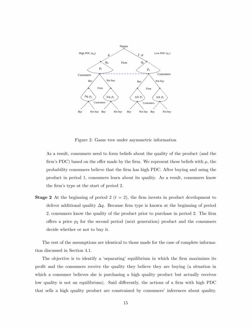
Figure 2):
Stage 1 Nature chooses the firm type, either high () or low () quality. As noted earlier,
firm type is perfectly correlated with PDC. The firm then chooses 1 for the first period
product. The consumers cannot evaluate quality (nor do they observe the firm type).
11Many researchers have considered various means of signaling quality: advertising (Milgrom and Roberts
1986), price (Choi 1998) and warranties (Soberman 2003). Price as a signal may be distorted either upward
(e.g., Choi 1998) or downward (Milgrom and Roberts 1986) to signal higher quality.12This is a reasonable assumption since the quality of the original product is also a result of the efforts
of the developers, technical personnel and facilities employed by the firm for the development of the second
generation product. We assume that the quality of those resources is highly correlated over time.13Note that since , we have ≤ 2
1−+(−)
1−−(−) + 2
1−+(−)
1−−(−) + ≤
.
14
Nature
High PDC (aH) Low PDC (aL)
Customers
Firm
Customers
Firm
µ 1- µ
qH qL
Customers
p1 p1
q, p2, q, p2
Buy Not buy
Buy Not buy Buy Not buy
Firm
Customers
Buy Not buy
Buy Not buy Buy Not buy
q, p2 q, p2
Figure 2: Game tree under asymmetric information
As a result, consumers need to form beliefs about the quality of the product (and the
firm’s PDC) based on the offer made by the firm. We represent these beliefs with , the
probability consumers believe that the firm has high PDC. After buying and using the
product in period 1, consumers learn about its quality. As a result, consumers know
the firm’s type at the start of period 2.
Stage 2 At the beginning of period 2 ( = 2), the firm invests in product development to
deliver additional quality ∆. Because firm type is known at the beginning of period
2, consumers know the quality of the product prior to purchase in period 2. The firm
offers a price 2 for the second period (next generation) product and the consumers
decide whether or not to buy it.
The rest of the assumptions are identical to those made for the case of complete informa-
tion discussed in Section 4.1.
The objective is to identify a ‘separating’ equilibrium in which the firm maximizes its
profit and the consumers receive the quality they believe they are buying (a situation in
which a consumer believes she is purchasing a high quality product but actually receives
low quality is not an equilibrium). Said differently, the actions of a firm with high PDC
that sells a high quality product are constrained by consumers’ inferences about quality.
15

We introduce this constraint in the high PDC firm’s optimization problem. This leads to a
standard signaling game in which the uninformed player (the consumer) makes an inference
about the type of the informed player (the firm) based on the latter’s action.
A key assumption in the analysis is that consumers know that the firm can have two
levels of PDC and the absolute levels associated with each type are common knowledge, i.e.,
consumers know the firm’s cost function for increasing quality and they also know that the
= or . To signal higher quality, the high PDC firm changes its first period offer as
explained in Proposition 2.
Proposition 2 When product quality is unobservable, the high PDC firm signals its type by
offering a lower price (1 = ) to myopic consumers in period 1 compared to the case of
complete information. The actions of a firm with low PDC are unaffected.
Proposition 2 shows that a firm with high PDC charges a lower price compared to the
price when product quality is observable. In fact, Proposition 2 implies that this price is
the same as the complete information price of a firm with low PDC which results in a “tie”.
However, the high PDC firm can drop the price by an arbitrarily small amount 0 (i.e.,
1 = −) at which the low PDC firm is strictly worse off thereby breaking the tie. The lowPDC firm does not mimic this strategy because it is unprofitable. Thus, its actions identify
it as a firm with low PDC because it charges the price (and employs the strategy) used under
complete information.
Signaling allows a high PDC firm to identify itself in period 1. In period 2, it charges the
complete information price because its type is known. This implies that a high PDC firm
will charge lower prices for new (first generation) products when quality is unobservable. The
impact of a high PDC firm charging lower prices is summarized in Proposition 3.
Proposition 3 When quality is unobservable and the quality in period 1 is above a threshold
( ≥ ), the high PDC firm covers the market early to signal its type and restricts sales of
the new generation product to the Highs in period 2 (“Market penetration” strategy). Note
that when quality is observable, a firm with high PDC does not employ first period “Market
penetration”.
Under complete information, a firm with high PDC focuses on the Highs in period 1 and
in period 2, it sells the product broadly (to Highs and Lows). Conversely, when consumers
16

cannot observe quality, the strategy of the high PDC firm changes. Proposition 3 implies
that the high PDC firm signals its type by offering a lower price in period 1 and this makes
the first generation product attractive to the Lows as well as the Highs. Then in period 2, the
high PDC firm restricts sales to the Highs.14 In summary, asymmetric information (and the
corresponding need to signal) causes a firm with high PDC to completely reverse the launch
strategy it would use were quality observable (broad then narrow versus narrow then broad).
It is also useful to underline why a firm with low PDC does not mimic the pricing of the
firm with high PDC. To be specific, there is nothing to stop a low PDC firm from copying
the high PDC firm’s price: this would lead to much first period demand as the firm would
sell to the Lows as well as the Highs. However, the main objective of a low PDC firm is to
maximize earnings from the endowed quality of the first generation product (high product
development costs make it infeasible to offer a significant quality improvement in period 2).
Were the low PDC firm to mimic the offer of the high PDC firm, it would lose the ability to
intertemporally discriminate between the Lows and Highs. Moreover, a small improvement
in product quality is naturally offered with a very low price to consumers who already have a
product (all consumers have a first generation product with the high PDC strategy described
in Proposition 3).
The model highlights who gains and loses when the quality of products is unobservable.
The primary loser is the firm with high PDC. In a nutshell, signaling costs money and firms
with high PDC (and hence higher quality first period products) need to signal. The primary
beneficiaries of asymmetric information are the Highs. When product quality is high, the
Highs are able to buy products with an attractive price that is essentially discounted by the
seller.
5 Consumers are Forward Looking
In this section we evaluate firm decisions in the same market but where the consumers are
“forward looking”, i.e., the consumers maximize their utility across the two periods based on
rational expectations about the firm’s price and quality decisions in period 2. As in the case
of myopic consumers, we first consider the case where quality is observable.
14When , the firm has low PDC and the optimal strategy is market inversion.
17
5.1 Quality is Observable
A forward looking consumer with rational expectations buys the product in period 1 if and
only if she expects a higher net surplus compared to waiting and purchasing in period 2. For
the Lows and Highs respectively, this implies 1 − 1 + 1 ≥ (2 − 2) and 1 − 1 +
1 ≥ (2 − 2). We now write the utility for the Lows and Highs in terms of the product
improvement ∆ made to the second generation product:
1 ( = ) = max{1 − 1 + 1 ( (1 +∆)− 2)} for Lows,1 ( = 1) = max{1 − 1 + 1 (1 +∆ − 2)} for Highs. (13)
Using the conventions of Section 4.1, we write the corresponding indicator functions in case
of forward looking Lows (Highs) as
=
½1 if 1 − 1 ≥ (∆ − 2)
0 otherwiseand 1 =
½1 if 1 − 1 ≥ (∆ − 2)
0 otherwise (14)
The second period utility from purchase is the same as for myopic consumers given by equation
8. Aside from the value consumers obtain by using the first period product, the model is very
similar to the specification of Section 4.
The market demand and firm profit functions are identical to those of Section 4.1.
Extensive Form of the Game: The timing of the game is identical to that of Section 4.1.
Only the basis for consumer decisions changes when consumers think ahead.
While the firm strategies remain the same as in Section 4.1 and equation 6, the necessary
conditions (or pricing constraints) for each strategy are different and this reflects the forward
looking decision basis that consumers use to make decisions.15
a) Market penetration: ( = 1 1 = 1), and ( = 0 1 = 1). The necessary conditions
are 1 − 1 ≥ (∆ − 2) ⇔ 1 ≤ 1 − (∆ − 2) and ∆ 2 ≤ ∆. The firmdecision problem, therefore, is
= max12∆
s.t. 1 − (∆ − 2)− 1 ≥ 0, and ∆ − 2 ≥ 0. (15)
15See Figure 4 in the Appendix.
18

b) High-end focus and then mass market : ( = 0 1 = 1), and ( = 1 1 = 1). Here, the
conditions are 1 − (∆ − 2) 1 ≤ 1 − (∆ − 2) and 2 ≤ ∆ (1 +∆).
The firm decision problem, therefore, is
= max12∆
s.t. 1 − (∆ − 2)− 1 ≥ 0, and ∆ − 2 ≥ 0. (16)
c) Market inversion: ( = 0 1 = 1), and ( = 1 1 = 0). The necessary conditions
are 1 − (∆ − 2) 1 ≤ 1 − (∆ − 2) and ∆ 2 ≤ (1 +∆). The firm
decision problem, therefore, is
= max12∆
s.t. 1 − (∆ − 2)− 1 ≥ 0, and (1 +∆)− 2 ≥ 0. (17)
d) Mass market: ( = 1 1 = 1), and ( = 1 1 = 1). Here, the conditions are
1 ≤ 1 − (∆ − 2) and 2 ≤ ∆.16 The firm decision problem, therefore, is
= max12∆
s.t. 1 − (∆ − 2)− 1 ≥ 0, and ∆ − 2 ≥ 0. (18)
As earlier, we solve the firm decision problem for each of the above strategies and compare
the outcomes to find the strategy that maximizes profit. Proposition 4 describes the optimal
strategies for the firm as a function of when consumers are forward looking.
Proposition 4 Forward Looking Consumers: Under complete information, a firm hav-
ing PDC higher than the threshold ≥ (where = 211
1−−1−−(1−)+
1−+(2−)(1−)) sells to both Highs
and Lows in period 1 and only to the Highs in period 2 (“Market penetration” strategy).
A firm having PDC less than the threshold ( ) serves the Highs in both periods and the
Lows only in period 2 (“High-end focus and then mass market” strategy).
Proposition 4 shows that forward looking behavior by consumers leads to a lower WTP
for the first period product because consumers weigh the benefit of consuming today against
the cost of waiting to buy in period 2. The impact of this behavior by consumers hurts the
firm: forward looking behavior creates a durable goods monopoly problem (Coase 1972). The
Highs know that they would trade up in period 2, implying that the first period product is
purchased based only on its consumption in period 1. Because the firm is forced to charge
a lower price in period 1 (due to the forward looking behavior of consumers), both types of
16Notice that the first period prices are lower under all strategies in case of forward looking consumers.
19

consumers buy the first generation product. When this occurs, the optimal strategy for the
high PDC firm is to develop a higher quality second generation product targeted to the Highs
alone and charge a correspondingly higher price for it.
Conversely, the strategy shifts from Market inversion to High-end focus and then mass
market when a firm has low PDC. As with a high PDC firm (when consumers are forward
looking), the price that consumers are willing to pay in period 1 is driven downwards. Inde-
pendent of the strategy employed by the firm, this hurts firm profits. However, when a firm
has low PDC, the incremental increase in product quality in period 2 is small (because of
the high cost of product development). Accordingly, a firm with low PDC has an incentive
to get as much money as it can from its “endowed” first period quality. It accomplishes
this by only selling to the Highs in period 1. In a sense, this allows the low PDC firm to
charge higher prices in both periods. In period 2, it proves beneficial for the firm to sell the
new generation broadly. The Highs are interested in the improved performance of the new
generation product and the WTP of the Lows is driven by the total benefit provided by the
product as they did not buy in period 1.
In sum, the most important effect created by forward looking behavior by consumers is
that consumers (Highs and Lows) have a lower WTP in period 1. This has two consequences.
First, it reduces first period prices and constrains the firm independent of PDC. Second,
forward looking behavior by consumers brings the Lows into the market sooner when a firm
has high PDC. The high PDC firm wrestles with the choice of charging a price that the Lows
find acceptable and extracting surplus from the Highs. By serving the Lows in period 1, the
high PDC firm unshackles itself in period 2 and is able to charge the Highs a high maximum
price for a “significantly improved” second generation product.
In contrast, the firm with low PDC extracts the maximum price in period 1 (from the
Highs) and then serves both Highs and Lows in period 2. Interestingly, when consumers
are forward looking, the Highs buy in every period independent of the PDC of the firm. In
contrast, when consumers are myopic, the Highs remain with the first generation product
when the firm has low PDC.
5.2 Quality is Unobservable
As in Section 4.2, we consider a situation where the firm cannot convey credible information
about product quality before consumers make their first purchase. Similar to the previous
20

section, consumers think about their expected second period benefits while making their
period 1 decision. Because consumers will make inferences about product quality when it is
not observable, a firm may be able to signal its quality through pricing.
Firm Types: Aside from the following assumption, firm types are identical to those
for myopic consumers as described in Section 4.2. We assume that (1 = ) and
(1 = ) to ensure that the optimal strategies of the high PDC firm and low PDC
firms are market penetration high-end focus and then mass market respectively, when quality
is observable. When either (1 = ) or (1 = ) , both
types of firms pursue the same strategy under complete information, and the high PDC firm
cannot signal its quality. Similar to Section 4.2, parameter conditions where the strategies of
the two types of firms under complete information are different lead to signalling.
Extensive Form of the Game: The timing of the game is identical to that of Section
5.1 except for the following: in Stage 1, Nature chooses the firm type either high () or
low () quality and consumers form beliefs with probability that the firm has high PDC.
Similar to Section 4.2, consumers become informed about the firm’s type before the second
period. Proposition 5 explains the optimal firm strategy when consumers are forward looking
but cannot observe product quality.
Proposition 5 When quality is unobservable and consumers are forward looking, the high
PDC firm signals its quality by offering a lower price (1 = 1 ) than under complete infor-
mation, but using the same “Market penetration” strategy as under complete information.
The actions of a firm with low PDC are unaffected.
When quality is unobservable, a high PDC firm offers a lower price in period 1 to signal
its quality. This finding echoes the equilibrium that obtains when consumers are myopic
and quality is unobservable (see Proposition 2). There is an important difference, however.
Other than charging a lower price (due to the need to make the signal informative), the
launch strategy of the high PDC firm is unaffected by the observability of quality.17 That
is, a firm with high PDC utilizes a strategy of market penetration independent of whether
quality is observable. This points to an important interaction between the way that consumers
think about their purchase decision and the observability of quality. When consumers think
myopically about decisions, quality being unobservable changes the optimal strategy of a
17The high PDC firm reduces its price to the point at which the low PDC firm does not have an incentive
to pretend to be high PDC when quality is not observable.
21

firm with high PDC (the high quality firm has ≥ ) from High-end focus and then
mass market to Market penetration. In contrast, when consumers are forward looking, the
strategy of a firm with high PDC is unaffected; only the price is different. Perhaps the
most interesting finding with regard to the impact of consumers thinking ahead (for their
first purchase decision) is the effect it has on the Lows when firms have high PDC. Forward
thinking behavior brings the Lows into the market sooner when a firm has high PDC. The
basic force driving this finding is the desire of the high PDC firm to capitalize on selling the
second generation product to the Highs. The sooner, the Lows are served (and effectively
removed from the market), the greater the flexibility of the high PDC firm to capitalize on
the high WTP of the Highs for the next sale.
6 Conclusions
The objective of this paper is to examine how the PDC of a firm that sells upgradable durable
goods affects marketing and product development decisions in a market where consumers
have heterogeneous valuations for performance. Under complete information, the optimal
marketing strategy of a firm having a high PDC revolves around selling (and re-selling) to
high WTP consumers. Here, extracting value for new product generations from high WTP
consumers is critical. This finding may explain why well-known makers of high end consumer
electronics (such as Sony, Apple, and Royal Philips Electronics) and sporting equipment such
as Völkl (skis) and Graf (hockey skates) make ongoing investments in product development
to develop new generations on a regular basis. The firm’s efficiency at developing higher
levels of performance makes offering new generations on a regular basis attractive.
In contrast, the optimal strategy of firms with low PDC is to focus on expanding the
market after serving high WTP consumers in period 1. Because firms with low PDC improve
their products less over time, they expand the market over time in order to optimize prof-
itability. Under certain conditions, the strategy of selling to as many consumers as possible
leads to “market inversion”: the firm serves high WTP consumers with early versions of the
product and low WTP consumers buy improved versions. In this case, high WTP consumers
continue to use old technology even when a newer version of the product is available.
Typically a firm sells the high and low quality products, respectively, to high and low
WTP consumers (see, for example, Maskin & Riley 1984). A phenomenon similar to mar-
ket inversion known as “vintage effects” has been noted in the literature (see for example,
22

Bohlmann, Golder and Mitra 2002). When two competing firms enter a market sequentially,
the follower uses more recent technology than an incumbent who has committed to older
technology. Thus an established market leader is sometimes observed to use less efficient
technology (an earlier vintage) than a new entrant. Of course, consistent with our findings,
this situation occurs when the new generation product offers a small advantage over the
original technology.
In some cases, it is difficult for consumers to evaluate the quality of a new product. For
example, many buyers of consumer electronics or specialized sporting equipment appreciate
their performance only after having used the product. This is the case when an unknown firm
or a firm “without a track record” launches a product that provides unique value. In these
situations, a firm with high PDC will signal its higher performance by offering its products
at a lower price than the optimal price charged by a firm with low PDC. This leads to mass
sell-in for the new product in period 1. In the second period, the firm restricts sales of the
new generation product to high WTP consumers. In a nutshell, this is a reversal of the
strategy used by a firm with high PDC under complete information.
It is important to note that the offering of a firm with low PDC is not affected by the
unobservability of product quality. Why does a low PDC firm not mimic the strategy of
the high PDC firm and pretend to be higher quality? The reason is that a firm with low
PDC optimizes its profit by intertemporally discriminating between high and low WTP. Said
differently, the low PDC firm needs to focus on maximizing earnings from the endowed quality
of the first generation product because the second generation product is only marginally better
than the first generation. If the low PDC firm mimics the high PDC firm, it loses the ability
to intertemporally discriminate between low and high WTP consumers. This obtains because
its type is common knowledge by the time consumers decide whether to buy in the second
period.
We also examine how forward looking behavior on the part of consumers affects the
launch strategy of firms as a function of the firm’s PDC. We show that forward looking
behavior causes a firm with high PDC to implement a marketing strategy that better aligns
the consumer valuations of product quality and the relative quality of products they consume.
In other words, rational expectations of consumers about future products causes a high PDC
firm to sell earlier versions of products more broadly (across consumer types) and improved
versions only to high WTP consumers. In period 2, low WTP consumers do not trade
23

up while the high WTP consumers trade up to the second generation product. Finally, we
examine how the strategy of a high PDC firm is affected by “hidden quality” when consumers
think ahead. Interestingly, “hidden quality” does not qualitatively alter the high PDC firm’s
marketing strategy; its only effect is to reduce the price of high quality products in period 1
as a high PDC firm “signals” its quality to the market.
Our research shows that product development capability has a significant impact on the
marketing strategy a firm should adopt to launch a product in a market where there is
significant heterogeneity with regard to consumers’ valuation of product performance. In
general, firms develop their marketing strategies after products have been developed. After
all, why spend time developing a marketing strategy for a product that is not ready?
Our analysis shows that this approach to product development and marketing is not
optimal. In particular, the optimal price of the first generation product is affected significantly
by a) the PDC of the firm, b) whether consumers assess future benefits when making current
decisions, and c) the ease with which consumers can evaluate the quality of a new product.
Moreover, the optimal level of investment in product improvement is impacted by the optimal
pricing and expected demand for the improved product. When a firm develops sequential
generations of a durable product for a heterogeneous market, our study underlines the benefits
of utilizing an integrated approach for these two activities. The following table summarizes
the optimal strategies of the firm under different conditions analyzed in our model.
Table 2: Summary of Optimal Strategies as a Function of PDC
Consumers→ Myopic Forward-looking
Quality→Firm ↓ Observable Hidden Observable Hidden
High PDCHigh-end focus &
then mass market
Market
penetration
Market
penetration
Market
penetration
Low PDCMarket
inversion
Market
inversion
High-end focus &
then mass market
High-end focus &
then mass market
Our study also suggests new areas of future research. One of them is to analyze how
competition between firms might affect the results. The model we have presented concerns
a monopolistic seller that sells to two segments over time that are different in terms of
willingness to pay. Using this structure as a starting point, competition might enter the
24

problem in two ways. First, competition might result in a reduction of the premium consumers
are willing to pay for a firm’s product. This would reduce firm incentives to invest in product
development. Second, firms might choose to focus on the high or low WTP consumers as
a function of their product development capability. Another interesting avenue to explore
would be the reactions of an incumbent that has the option of selling in both periods but is
faced with a second period entrant whose quality might be high or low.
25

References
[1] Abernathy, W.J. and J.M. Utterback (1978). Patterns of Industrial Innovation. Technol-ogy Review, 80(7), 40-47.
[2] Akerlof, G.A. (1970). Market for “Lemons”: Quality Uncertainty and the Market Mech-anism. Quarterly Journal of Economics, 84(3), 488-500.
[3] Balachander, S. and K. Srinivasan (1994). Selection of Product Line Qualities and Pricesto Signal Competitive Advantage. Management Science. 40(7), 824-841.
[4] Banerjee, S. and M. Sarvary (2009). How Incumbent Firms Foster Consumer Expecta-tions, Delay Launch but still Win the Markets for Next Generation Products. Quanti-tative Marketing and Economics, 7 (4), 445-481.
[5] Bohlmann, J.D., P.N. Golder and D. Mitra (2002). Deconstructing the Pioneer’s Ad-vantage: Examining Vintage Effects and Consumer Valuations of Quality and Variety.Management Science, 48 (9), 1175—1195.
[6] Coase, R.H. (1972). Durability and Monopoly. Journal of Law and Economics, 15, 143-49.
[7] Cho, I.K and D.M Kreps (1987). Signaling Games and Stable Equilibria. QuarterlyJournal of Economics, 102(2), 179-221.
[8] Choi, J.P (1998). Brand Extensions as Informational Leverage. The Review of EconomicStudies, 65 (4), 655-669.
[9] Dhebar, A. (1994). Durable-goods monopolists, rational consumers, and improving prod-ucts. Marketing Science. 13 (1), 100-120.
[10] Ellison, G. and D. Fudenberg (2000). The Neo-Luddite’s Lament: Excessive Upgradesin the Software Industry. The RAND Journal of Economics, 31(2), 253-272
[11] Fudenberg, D. and J. Tirole (1991). Game Theory. Cambridge MA: MIT Press.
[12] Fudenberg, D. and J. Tirole (1998). Upgrades, Tradeins, and Buybacks. The RANDJournal of Economics, 29(2), 235-258.
[13] Hendel I. and A. Lizzeri (1999). Adverse Selection in Durable Goods Markets. AmericanEconomic Review, 89 (5), 1097-1115.
[14] Koenigsberg, O., R. Kohli and R. Montoya (2011). The Design of Durable Goods. Mar-keting Science. 30 (1), 111-122.
[15] Kornish, L. (2001). Pricing for a Durable-Goods Monopolist Under Rapid SequentialInnovation. Management Science. 47(11), 1552-1561.
[16] Krishnan, V. andW. Zhu (2006). Designing a Family of Development-Intensive Products.Management Science, 52: 813-825.
[17] Langinier, C. (2005). Using Patents to mislead rivals, Canadian Journal of Economics,38 (2), 520-45.
[18] Maskin, E. and J. Riley (1984). Monopoly with Incomplete Information.The RANDJournal of Economics. 15(2), 171-196.
26

[19] Milgrom, P.R. and J. Roberts (1986). Prices and Advertising Signals of Product Quality.Journal of Political Economy. 94 (4), 796-821.
[20] Moorthy, K.S. and I.P.L Png. (1992). Market Segmentation, Cannibalization, and theTiming of Product Introductions. Management Science. 38(3), 345-359.
[21] Ofek, E. (2008). Sony PlayStation 3: Game Over? Harvard Business Case.
[22] Ofek, E. and M. Sarvary (2003). R&D, Marketing, and the Success of Next-GenerationProducts. Marketing Science, 22(3), 355—370.
[23] Padmanabhan, V., S. Rajiv and K. Srinivasan (1997). New Products, Upgrades andNew Releases: A Rationale for Sequential Product Introduction. Journal of MarketingResearch, 34 (4), 456-472.
[24] Purohit, D. (1994). What should you do when your competitors send in the clones?Marketing Science. 13 (4), 392-311.
[25] Ramachandran, K. and V. Krishnan (2008). Design Architecture and Introduction Tim-ing for Rapidly Improving Industrial Products. MSOM, 10(1), 149-171.
[26] Shankaranarayanan, R. (2007). Innovation and the Durable Goods Monopolist. Market-ing Science. 26 (6), 774-791.
[27] Soberman, D.A. (2003). Simultaneous Signaling and Screening with Warranties. Journalof Marketing Research, 40 (2), 176-192.
[28] Waldman, M. (2003). Durable Goods Theory for Real World Markets. Journal of Eco-nomic Perspectives, 17 (1), 131-154.
[29] Weitzman, M.L., W. Newey and M. Rabin (1981). Sequential R&D Strategy for Synfuels.The Bell Journal of Economics, 12 (2), 574-590.
[30] Yin, S., S. Ray, H. Gurnani and A. Animesh (2010). Durable Products with Multi-ple Used Goods Markets: Product Upgrade and Retail Pricing Implications. MarketingScience. 29 (3), 540-560.
27

Appendix
Derivation of Condition 1
Consider the firm decision in period 1. If the firm sells only to the Highs ( = 0 1 = 1),the firm chooses a price 1 = 1 and obtains a demand of 1 = 1− . On the other hand, ifit sells to both types of consumers ( = 1 = 1), it chooses a price 1 = 1 and obtains ademand of 1 = 1. We can see that the firm earns less profit from selling only to the Highsunless (1− ) (1 − ) ≥ 1 − where is the marginal cost. This condition is triviallysatisfied as long as 1− ≥ .
Derivation of Condition 2
Due to condition 1, the firm serves only the Highs in period 1 ( = 0 1 = 1). Consider nowthe firm decision in period 2. If ∆ ≥ (1 +∆) in violation of condition 2, the firm canpossibly earn higher profits by charging a higher price equal to ∆ at which only the Highsbuy ( = 0 1 = 1), leading to a demand 2 = 1− because 1− ≥ (condition 1). TheLows are therefore not served.
On the other hand, when ∆ (1 +∆), if the firm charges a higher price equal to (1 +∆), only the Lows buy ( = 1 1 = 0), leading to a demand 2 = . Alternatively,it can charge a lower price equal to∆ at which both types of consumers buy ( = 1 1 = 1),leading to a higher demand 2 = 1. Therefore, if the firm has any demand at all in period2, it is guaranteed that the Lows buy when ∆ (1 +∆). In other words, if 2 0, = 1 is assured under the sufficient (but not necessary) conditions 2 and 1.
Proof of Proposition 1
We solve the firm’s constrained optimization problem for each of the decision alternativesand then compare the profit values across all the strategic alternatives. Figure 3 illustrates acharacterization of the market outcomes as a function of the prices of the two periods. Weapply the Kuhn-Tucker necessary and sufficient conditions for global maximum for each ofthe four strategies below as the objective function is concave and the constraints are linear.
Market penetration Substituting {= 1= 1}⇒ 1= 1, and {1= 1 = 0}⇒ 2= 1− ,in equations 6 and 9, we get the Lagrangian
L = 1+ (2−∆) (1− )−∆2+21∆
2−1 (1−1)−2 (2−∆)
where 1≥ 0 2≥ 0.The Kuhn-Tucker conditions are
Marginal Condition Complementary SlacknessL1= 1− 1≤ 0 L
11= 0
L2= (1− )−2≤ 0 L
22= 0
L∆
= − (1− )− ∆+1
+2≤ 0 L
∆∆= 0
L1= 1 − 1 ≥ 0 L
11= 0
L2= ∆ − 2≥ 0 L
22= 0
Solving the marginal conditions, we get 1= 1, 2= (1− ),∆∗= (1− ) (1− )−1,∗1= 1, and ∗2= (1− ) (1− )−1. The resulting firm profits are:
∗= 1 + [ (1− ) (1− )−1]2
2 (A.1)
i

Mass Market
Market Penetration
High-end Focus & then Mass
Market
Market Inversion
No sales to low-type consumers in t=2
No sales to low-type consumers in
t=1 No sales in t=2
No sales in t=1
No market
First Period Price
Second Period Price
p2
p1
1q 1q
q
q
qq 1
qq 1
Figure 3: Characterization of market outcomes as a function of prices when consumers are
myopic
High-end focus and then mass market Substituting {= 0 1= 1}⇒ 1= 1− , {1= 1 = 1}⇒ 2= 1, in equations 6 and 10, we get the Lagrangian
L = 1 (1− )+ (2−∆)−∆2+21∆
2−1 (1−1)−2 (2−∆)
where 1≥ 0 2≥ 0.
The Kuhn-Tucker conditions are
Marginal Condition Complementary SlacknessL1= 1− − 1≤ 0 L
11= 0
L2= − 2≤ 0 L
22= 0
L∆
= −− ∆+1
+2≤ 0 L
∆∆= 0
L1= 1 − 1 ≥ 0 L
11= 0
L2= ∆ − 2≥ 0 L
22= 0
Solving the marginal conditions, we get 1= 1− , 2= , ∆∗= (1− )−1, ∗1= 1,and ∗2= (1− )−1. The resulting profits are:
∗= (1− ) 1 + [ (1− )−1]2
2 (A.2)
Market inversion Substituting {= 0 1= 1}⇒ 1= 1− , {1= 0 = 1}⇒ 2= , inequations 6 and 11, we get the Lagrangian
L = 1 (1− )+ (2−∆)− ∆2+21∆
2−1 (1−1)−2 [2− (1 +∆)]
where 1≥ 0 2≥ 0.
ii

The Kuhn-Tucker conditions are
Marginal Condition Complementary SlacknessL1= 1− − 1≤ 0 L
11= 0
L2= − 2≤ 0 L
22= 0
L∆
= −− ∆+1
+2≤ 0 L
∆∆= 0
L1= 1 − 1 ≥ 0 L
11= 0
L2= (1 +∆)− 2≥ 0 L
22= 0
Solving the marginal conditions, we get 1= 1− , 2= , ∆∗= ( − ) − 1,∗1= 1, and ∗2= (1 + ( − )− 1). The resulting profits are:
∗=(1− (1− )) 1 + [ ( − )−1]2
2 (A.3)
Mass market Substituting {= 1= 1}⇒ 1= 1, {1= 1 = }⇒ 2= 1 in equations 6and 12, we get the Lagrangian
L = 1+ (2−∆)−∆2+21∆
2−1 (1−1)−2 [2−∆]
where 1≥ 0 2≥ 0.
The Kuhn-Tucker conditions are
Marginal Condition Complementary SlacknessL1= 1− 1≤ 0 L
11= 0
L2= − 2≤ 0 L
22= 0
L∆
= −− ∆+1
+2≤ 0 L
∆∆= 0
L1= 1 − 1 ≥ 0 L
11= 0
L2= ∆ − 2≥ 0 L
22= 0
Solving the marginal conditions, we get 1= 1, 2= , ∆∗= ( − )−1, ∗1= 1,and ∗2= ( ( − )− 1). The resulting profits are:
∗= 1 + [ ( − )−1]2
2 (A.4)
We now identify the firm strategy that results in the market outcome yielding maximumprofits. As before, comparing profits above we can see that ∗ ∗ ∗ due toequation 1. Comparing ∗ and ∗ we can see that
∗ ≥ ∗ only if ≥ where
=21
1− + ( − )
µ
1− − ( − )+
¶ (A.5)
Therefore, High-end focus and then mass market is the optimal strategy of the firm if ≥ . On the other hand if , Market inversion is the optimal strategy. Q.E.D.
iii
Proof of Proposition 2
The Equilibrium Concept: To solve the game, we use Perfect Bayesian Equilibrium (PBE)concept. The PBE leads to a unique outcome when:
(P) The strategies of the informed player are optimal given the beliefs of the uninformed players.
(B) The beliefs of uninformed players are based on strategies that are consistent with Bayes’ Rule.
The PBE imposes a rule of “logical consistency” on the beliefs of uninformed players (Fuden-berg and Tirole 1991); that is, the beliefs of uninformed players (i.e., consumers) are derivedusing Bayes’ Rule from the actions of the informed player (the firm) before the uninformedplayer makes a decision. We assume that ∈ [0 1] is consumers’ prior belief that the firmhas high PDC, having observed the firm action or signal 1 and (1) is their posterior
belief. The triplet©∗1 ∗1
ªconstitutes a Perfect Bayesian Equilibrium (PBE) if and
only if it satisfies the following conditions related to sequential rationality (P) and Bayesianconsistency in beliefs (B).
(P) ∗1 ∈ argmax1
(1 (1))
(B) If ∗1 = ∗1 = ∗1 then (∗1)= . (Pooling Equilibrium)
If ∗1 6=∗1 then ¡∗1
¢= 1 and
¡∗1¢= 0. (Separating Equilibrium)
In this game there are two possible equilibria types. In a pooling equilibrium, consumerscannot update their prior belief by observing only the price since both high and low typefirms charge the same price. Conversely, in a separating equilibrium consumers can identifythe firm type because the two types of firms charge different prices. PBE only imposes logicalconsistency on the beliefs of the players over actions on the equilibrium path; there are norestrictions on the beliefs of the players over actions off the equilibrium path. In signalinggames, freedom in specifying off-equilibrium beliefs can lead to multiple equilibria when theoff-equilibrium beliefs of uninformed players attribute positive probability to the informedplayer (the firm) choosing an equilibrium-dominated strategy. The Intuitive Criterion (IC)of Cho and Kreps (1987) eliminates these equilibria by imposing a restriction on the players’beliefs over actions off the equilibrium path.
Intuitive Perfect Bayesian Equilibrium
A PBE violates the intuitive criterion if there exists an action that yields strictly greaterpayoffs for a player given that the uninformed players ascribe zero probability to a player’saction that is “equilibrium-dominated”. An action is “equilibrium-dominated” for a playerif that action leads to lower profits than another putative equilibrium. In other words, afirm type choosing an “equilibrium-dominated” action cannot increase its profit over what itearns under equilibrium.
In the context of this model, the beliefs of consumers subject to the IC restrict the highPDC firm to a set of strategies
¡1¢which is equilibrium dominated for a firm with low
PDC: were it to implement a strategy from this set, the low PDC firm would earn less thanits “guaranteed” level of profit. The only equilibrium that survives the intuitive criterion is aseparating equilibrium with minimal inefficient signaling. In addition, a high PDC firm has aprofit-increasing deviation from all possible pooling equilibria when signaling is possible.1 Theguaranteed profit for the low PDC firm, is the profit it earns when consumers can observequality. The low PDC firm has an incentive to mimic a high PDC firm if it increases profit byoffering 1 : the offer that would be made by a firm with high PDC, i.e.,
¡1 = 1
¢ .
In equilibrium, the intuitive criterion rules out these strategies for the high PDC firm. Asnoted earlier, the intuitive criterion is the basis for the following constraint in the high PDCfirm’s optimization:
¡1 = 1
¢ (A.6)
1When a signal is either costless or inexpensive, signaling may be impossible.
iv

Note that a high PDC firm should not be able increase profits by pretending to be a firmwith low PDC, i.e.,
¡1 = 0
¢ (A.7)
Because , this restriction is satisfied.The “guaranteed” profit of the low PDC firm is the profit it earns when it offers the price
∗1 which is the optimal price of the low PDC when quality is observable. The guaranteedprofit, is obtained by substituting = and 1 = into the firm’s profit function andoptimizing.
All Putative Pooling Equilibria are Unstable based on the Intuitive Criterion
Recall from Proposition 1 that the optimal strategy for the high (low) PDC firm is High-endfocus and then mass market (Market inversion). When quality is unobservable, if the highPDC firm offers the same price which is also the maximum price it can charge as undercomplete information (∗1 (1 = 1 1 = )= ), it would violate the “no-mimic condition”(equation A.6). This implies that a firm with low PDC will have an incentive to offer thesame price as that of the high PDC firm which would result in a pooling equilibrium. Weshow below, using the Intuitive Criterion, that a pooling equilibrium does not exist.
Suppose there is a putative pooling equilibrium (∗1) in which the consumers accept thefirst period price given the expected quality (1)= +(1− ) given ∗1 ≤ (1).
Step 1 First, we can find a deviation combination¡ = ∗1 +
¢such that
¡1 = 1
¢= ∗ (
∗1 ) (A.8)
where ¡1 = 1
¢= ∗
¡∗1 = 1 1 = =
¢and
∗ (∗1 ) = ∗ (
∗1 1 = = )
From the optimization in the Proof of Proposition 1, we can see that ∗
¡∗1 = 1 1 = =
¢= (1− ) (∗1 +)+
[(1−)−]22
and ∗ (∗1 1 = = ) = (1− ) ∗1+
[(−)−]22
where solves ∗
¡∗1 = 1 1 = =
¢= ∗ (
∗1 1 = = ). Now, con-
sidering a deviation price −1 which is infinitesimally less profitable than 1 , i.e.,
−1 = ∗1+ − , we have the low PDC firm’s profit − ∗. Thus at the price−, the low PDC firm earns strictly less profit than the equilibrium profit ∗ (
∗1 )
implying the price − is equilibrium dominated for the low PDC firm. According tothe Intuitive Criterion, consumers cannot ascribe positive probability to a firm typechoosing a strategy that is equilibrium dominated. Therefore, the posterior probabilityof the consumers (−)= 1.
Step 2 Using this price¡1¢, the profit of the high PDC firm is = ∗
¡∗1 = 1 1 = =
¢ ∗ (
∗1 ) (because (1= ) (1= ) ). Therefore if the high PDC
firm offers a price infinitesimally lower, i.e., −1 , this price will still yield a positive
profit − (∗1 ). Thus the price
−1 is not equilibrium dominated for the high
PDC firm. The high PDC firm can increase its profits by offering a deviation price
−1 and convince the consumers that it has a high PDC and also earn a higher profit.Thus, there can be no intuitive pooling equilibrium. Q.E.D.
Separating Equilibrium for Myopic ConsumersWe consider a separating equilibrium when quality is unobservable. We first obtain the no-mimic condition from the optimization problem of the low PDC firm when (1 = )
v

using the separating price 1 as given below.2 Solving the game backwards, its second period
pricing decision is
¡1 = 1
¢=max2∆
¡1¢s.t. 2≤ (+∆) .
The Lagrangian is given by
L=(1− ) 1 + (2−∆)−∆2+2∆
2−1 (2− (+∆)) where 1≥ 0.
Kuhn-Tucker conditions yield 1 = 0, ∆= ( − )− and ∗2= (+∆) withresulting profits:
¡1 = 1
¢=(1− ) 1 ++
( ( − )−)22
(A.9)
Note that the low PDC firm mimics only if ¡1 = 1
¢ which is possible only if
1 where 1 ∈ [ ]. The no-mimic constraint is obtained by simplifying the condi-
tion ¡1 = 1
¢≤ where is obtained from the expression A.3 as given by
= [1− (1− )] + ( ( − )−)2
2 (A.10)
The no-mimic constraint therefore is given by
1 ≤ (A.11)
We solve the separating profit maximization problem of the high PDC ( (1 = ))
firm using the “no-mimic condition” (Equation A.11) as a constraint: 1 ≤ . This is givenby the optimization problem
∗¡1 = 1
¢= max1 2∆
( = 1= ) s.t. 1 ≤ .
Simplifying the Lagrangian only for the decisions 1 (note that the decisions 2 and ∆remain unchanged from the complete information case), we have
L = (1− ) 1 +( (1− )−)2
2−1
¡1 −
¢where 1≥ 0.
The Kuhn-Tucker conditions yield: 1= 1− 0 and ∗1 = . Note that this may lead
to a tie which is broken by the high PDC firm by charging ∗1 = − where 0 isinfinitesimally small. The separating profit for the high PDC firm therefore is
∗¡∗1 = 1
¢=(1− ) +
( (1− )−)22
Q.E.D.
2Note that since (1 = ), Market Inversion is the optimal strategy for the firm.
vi

MassMarket
Market Penetration
MarketInversion
No sales to low-type consumers in t=2
No sales to low-type consumers in
t=1 No sales in t=2
No sales in t=1
No market
First Period Price
Second Period Price
p2
p1
1q 1q
q
q
qq 1
qq 1
High-end Focus &
then Mass Market
Figure 4: Characterization of market outcomes as a function of prices when consumers are
forward looking
Proof of Proposition 3
If the quality of the high PDC firm is above a threshold given by the following condition, theLows buy in period 1
∗1 ≤ ⇔ ≥ . (A.12)
They do not, however, trade up in period 2 since the market penetration strategy is preferableto the mass market strategy, i.e., ∗ ∗ from Equations A.13 and A.16 under Proof ofProposition 1. Q.E.D.
Proof of Proposition 4
The solution approach is exactly the same as that in Proof of Proposition 1. Figure 4illustrates a characterization of the market outcomes as a function of the prices of the twoperiods. We apply the Kuhn-Tucker necessary and sufficient conditions for global maximumfor each of the four strategies below as the objective function is concave and the constraintsare linear.
Market penetration Substituting {= 1= 1}⇒ 1= 1, and {1= 1 = 0}⇒ 2= 1− ,in equations 6 and 15, we get the Lagrangian
L = 1+ (2−∆) (1− )−∆2+21∆
2−1 (1−1 + (∆ − 2))−2 (2−∆)
where 1≥ 0 2≥ 0.
vii

The Kuhn-Tucker conditions are
Marginal Condition Complementary SlacknessL1= 1− 1≤ 0 L
11= 0
L2= (1− )+1−2≤ 0 L
22= 0
L∆
= − (1− )− ∆+1
−1 + 2≤ 0 L
∆∆= 0
L1= 1 − (∆ − 2)− 1 ≥ 0 L
11= 0
L2= ∆ − 2≥ 0 L
22= 0
Solving the marginal conditions, we get 1= 1, 2= (2− ),∆∗= (1− +(1− ) (1− ))−1,∗1= 1 + (1− ) ( [1− +(1− ) (1− )]−1), and ∗2= [1− +(1− ) (1− )]−1.The resulting firm profits are:
∗= 1 + [ [1− +(1− ) (1− )]−1]2
2 (A.13)
High-end focus and then mass market Substituting {= 0 1= 1}⇒ 1= 1− , {1= 1 = 1}⇒ 2= 1, in equations 6 and 16, we get the Lagrangian
L = 1 (1− )+ (2−∆)−∆2+21∆
2−1 (1−1 + (∆ − 2))−2 (2−∆)
where 1≥ 0 2≥ 0.The Kuhn-Tucker conditions are
Marginal Condition Complementary SlacknessL1= 1− − 1≤ 0 L
11= 0
L2= + 1 − 2≤ 0 L
22= 0
L∆
= −− ∆+1
−1+2≤ 0 L
∆∆= 0
L1= 1 − (∆ − 2)− 1 ≥ 0 L
11= 0
L2= ∆ − 2≥ 0 L
22= 0
Solving the marginal conditions, we get 1= 1− , 2= + (1− ),∆∗= (1− )−1,∗1= 1, and ∗2= (1− )−1. The resulting profits are:
∗= (1− ) 1+ [ (1− )−1]2
2 (A.14)
Market inversion Substituting {= 0 1= 1}⇒ 1= 1− , {1= 0 = 1}⇒ 2= , inequations 6 and 17, we get the Lagrangian
L = 1 (1− )+ (2−∆)− ∆2+21∆
2−1 (1−1 + (∆ − 2))−2 [2− (1 +∆)]
where 1≥ 0 2≥ 0.The Kuhn-Tucker conditions are
Marginal Condition Complementary SlacknessL1= 1− − 1≤ 0 L
11= 0
L2= + 1 − 2≤ 0 L
22= 0
L∆
= −− ∆+1
−1+2≤ 0 L
∆∆ = 0
L1= 1 − (∆ − 2)− 1 ≥ 0 L
11= 0
L2= (1 +∆)− 2≥ 0 L
22= 0
viii

Solving the marginal conditions, we get 1= 1− , 2= . Note, here, that from the
marginal condition L∆≤ 0,∆ = ( − − (1− ))−1 0 under condition 1. Therefore,
from the complementary slackness, we get ∆∗= 0. From the rest of the marginal conditions,we get 1=(1 + ) 1, and 2= 1. Note, however, that since ∆
∗= 0, the forward lookingHighs will anticipate the subsequent drop in price to 1 in period 2, and therefore, defertheir purchase (Coase 1972) forcing the firm to charge ∗1= 1 and leading to profits:
∗= 1 (A.15)
Mass market Substituting {= 1= 1}⇒ 1= 1, {1= 1 = }⇒ 2= 1 in equations 6and 18, we get the Lagrangian
L = 1+ (2−∆)−∆2+21∆
2−1 (1−1 + (∆ − 2))−2 [2−∆]
where 1≥ 0 2≥ 0.
The Kuhn-Tucker conditions are
Marginal Condition Complementary SlacknessL1= 1− 1≤ 0 L
11= 0
L2= + 1 − 2≤ 0 L
22= 0
L∆
= −− ∆+1
−1+2≤ 0 L
∆∆= 0
L1= 1 − (∆ − 2)− 1 ≥ 0 L
11= 0
L2= ∆ − 2≥ 0 L
22= 0
Solving the marginal conditions, we get 1= 1, 2= 2, ∆∗= ( − ) − 1,
∗1= 1,
and ∗2= ( ( − )− 1). The resulting profits are:
∗= 1+ [ ( − )−1]2
2 (A.16)
We now identify the firm strategy that results in the market outcome yielding maximumprofits. Comparing profits above, we can see that ∗ ∗ ∗ and ∗ ∗due to equation 1. Comparing ∗ and ∗ we can see that
∗ ≥ ∗ . Next comparing
∗ with ∗ , we can see that ∗≥ ∗ only if ≥ where
= 21
1
1−−1−−(1−) +
1− +(2− ) (1− ) (A.17)
Therefore,Market penetration is the optimal strategy of the firm if ≥ . On the otherhand, ∗ ∗ if i.e., High-end focus and then mass market is the optimalstrategy. Q.E.D.
Proof of Proposition 5
The Equilibrium Concept: Is the same as stated under Proof of Proposition 2.
All Putative Pooling Equilibria are Unstable based on the Intuitive Criterion
Analogous to the case of myopic consumers (see Proof of Proposition 2), the proof that allputative pooling equilibria are unstable follows the same logic. Recall from Proposition 4 thatthe optimal strategy for the high (low) PDC firm is Market penetration (High-end focus and
ix

then mass market). If the high PDC firm offers the same price as under complete informa-tion, i.e., ∗1 (1 = 1 = = )= + (1− ) ( [1− +(1− ) (1− )]−), itwould violate the “no-mimic condition” (equation A.6) since the low PDC firm will have anincentive to offer the same price which would result in a pooling equilibrium. We show belowusing the Intuitive Criterion that a pooling equilibrium does not exist.
Suppose there is a putative pooling equilibrium (∗1) in which the consumers accept thefirst period price given the expected quality (1)= +(1− ) given ∗1 ≤ (1).
Step 1 First, we can find a deviation combination¡ = ∗1 +
¢such that
¡1 = 1
¢= ∗ (
∗1 ) (A.18)
where ¡1 = 1
¢= ∗
¡∗1 = 1 1 = =
¢and
∗ (∗1 ) = ∗ (
∗1 1 = = )
From the optimization in the Proof of Proposition 4, we can see that ∗
¡∗1 = 1 1 = =
¢=∗1++
[(1−)(1−)−]2−2(1−)22
and ∗ (∗1 1 = = ) = (1− ) ∗1+
[(1−)−]22
where solves ∗
¡∗1 = 1 1 = =
¢= ∗ (
∗1 1 = = ). Now, con-
sidering a deviation price −1 which is infinitesimally less profitable than 1 , i.e.,
−1 = ∗1+ − , we have the low PDC firm’s profit − ∗ since 0. Thus atthe price −, the low PDC firm earns strictly less profit than the equilibrium profit∗ (
∗1 ) implying the price − is equilibrium dominated for the low PDC firm. Ac-
cording to the Intuitive Criterion, consumers cannot ascribe positive probability to afirm type choosing a strategy that is equilibrium dominated. Therefore, the posteriorprobability of the consumers (−)= 1.
Step 2 Using this price¡1¢, the profit of the high PDC firm is = ∗
¡∗1 = 1 1 = =
¢ ∗ (
∗1 ) (because (1= ) (1= ) ). Therefore if the high PDC
firm offers a price infinitesimally lower, i.e., −1 , this price will still yield a positive
profit − (∗1 ). Thus the price
−1 is not equilibrium dominated for the high
PDC firm. The high PDC firm can increase its profits by offering a deviation price
−1 and convince the consumers that it has a high PDC and also earn a higher profit.Thus, there can be no intuitive pooling equilibrium. Q.E.D.
Separating Equilibrium for Forward-looking ConsumersTo identify the separating equilibrium, we first obtain the no-mimic condition from the op-timization problem of the low PDC firm using the separating price 1 . Solving the gamebackwards, period 2 pricing decision is
¡1 = 1
¢=max2∆
¡1¢s.t. 2≤ ∆.
The Lagrangian is given by
L=1 + (1− ) (2−∆)−∆2+2∆
2−1 (2−∆) where 1≥ 0.
Kuhn-Tucker conditions yield 1 = (1− ) 0, ∆ = (1− ) (1− )− and ∗2= ∆
with resulting profits:
¡1 = 1
¢= 1 +
[ (1− ) (1− )− ]2
2 (A.19)
x
Note that the low PDC firm mimics only if ¡1 = 1
¢ ∗ where
∗ = ∗ ( = 1 = ) = (1− ) + [ (1− )−]2
2 (A.20)
This condition simplifies to 1 1 where
1 = (1− ) + (1− )
∙
µ1−2
¶(1− )−
¸ (A.21)
Note from the optimization problem for Market penetration (equation A.13) that 1 ≤ ∗1(where ∗1 is the complete information price of the high PDC firm) is a necessary condition formimicking. Otherwise, the high PDC firm can separate using its complete information price
∗1. The no-mimic constraint therefore is given by 1 ≤ 1 . Solving the separating profitmaximization problem of the high PDC firm involves the “no-mimic condition” (EquationA.21) as a constraint. This is given by the optimization problem
∗¡1 = 1
¢= max1 2∆
( = 1 = ) s.t. 1 ≤ 1
Simplifying the Lagrangian only for the decisions 1 (note that the decisions 2 and ∆remain unchanged from the complete information case) and solving the marginal conditions,
we get: 1= 1− 0 and ∗1 = 1 . The separating profit for the high PDC firm thereforeis
∗¡∗1 = 1
¢= ∗1 +
[ [1− +(1− ) (1− )]− ]22
Note that both high and Lows buy in period 1 and henceMarket penetration is the optimalstrategy also under signaling. Q.E.D.
xi


