
NBER WORKING PAPER SERIES
PUBLIC MOBILITY DATA ENABLES COVID-19 FORECASTING AND MANAGEMENT AT LOCAL AND GLOBAL SCALES
Cornelia IlinSébastien E. Annan-Phan
Xiao Hui TaiShikhar Mehra
Solomon M. HsiangJoshua E. Blumenstock
Working Paper 28120http://www.nber.org/papers/w28120
NATIONAL BUREAU OF ECONOMIC RESEARCH1050 Massachusetts Avenue
Cambridge, MA 02138November 2020
The views expressed herein are those of the authors and do not necessarily reflect the views of the National Bureau of Economic Research.
NBER working papers are circulated for discussion and comment purposes. They have not been peer-reviewed or been subject to the review by the NBER Board of Directors that accompanies official NBER publications.
© 2020 by Cornelia Ilin, Sébastien E. Annan-Phan, Xiao Hui Tai, Shikhar Mehra, Solomon M. Hsiang, and Joshua E. Blumenstock. All rights reserved. Short sections of text, not to exceed two paragraphs, may be quoted without explicit permission provided that full credit, including © notice, is given to the source.

Public Mobility Data Enables COVID-19 Forecasting and Management at Local and GlobalScalesCornelia Ilin, Sébastien E. Annan-Phan, Xiao Hui Tai, Shikhar Mehra, Solomon M. Hsiang,and Joshua E. BlumenstockNBER Working Paper No. 28120November 2020JEL No. C1,C8,H12,H70,I18,O2,R40
ABSTRACT
Policymakers everywhere are working to determine the set of restrictions that will effectively contain the spread of COVID-19 without excessively stifling economic activity. We show that publicly available data on human mobility — collected by Google, Facebook, and other providers — can be used to evaluate the effectiveness of non-pharmaceutical interventions and forecast the spread of COVID-19. This approach relies on simple and transparent statistical models, and involves minimal assumptions about disease dynamics. We demonstrate the effectiveness of this approach using local and regional data from China, France, Italy, South Korea, and the United States, as well as national data from 80 countries around the world.
Cornelia IlinSchool of InformationUniversity of California at Berkeley [email protected]
Sébastien E. Annan-PhanAgricultural and Resource EconomicsUniversity of California, [email protected]
Xiao Hui TaiSouth HallUniversity of California, Berkeley Berkeley, CA [email protected]
Shikhar MehraSchool of Information University of California, [email protected]
Solomon M. HsiangGoldman School of Public Policy University of California, Berkeley 2607 Hearst AvenueBerkeley, CA 94720-7320and [email protected]
Joshua E. BlumenstockSchool of Information102 South HallUniversity of California, Berkeley [email protected]

Summary1
Background. Policymakers everywhere are working to determine the set of restrictions that will2
effectively contain the spread of COVID-19 without excessively stifling economic activity. In some3
contexts, decision-makers have access to sophisticated epidemiological models and detailed case4
data. However, a large number of decisions, particularly in low-income and vulnerable communities,5
are being made with limited or no modeling support. We examine how public human mobility6
data can be combined with simple statistical models to provide near real-time feedback on non-7
pharmaceutical policy interventions. Our objective is to provide a simple framework that can be8
easily implemented and adapted by local decision-makers.9
Methods. We develop simple statistical models to measure the effectiveness of non-pharmaceutical10
interventions (NPIs) and forecast the spread of COVID-19 at local, state, and national levels. The11
method integrates concepts from econometrics and machine learning, and relies only upon publicly12
available data on human mobility. The approach does not require explicit epidemiological modeling,13
and involves minimal assumptions about disease dynamics. We evaluate this approach using local14
and regional data from China, France, Italy, South Korea, and the United States, as well as national15
data from 80 countries around the world.16
Findings. We find that NPIs are associated with significant reductions in human mobility, and that17
changes in mobility can be used to forecast COVID-19 infections. The first set of results show the18
impact of NPIs on human mobility at all geographic scales. While different policies have different19
effects on different populations, we observed total reductions in mobility between 40 and 84 percent.20
The second set of results indicate that — even in the absence of other epidemiological information21
— mobility data substantially improves 10-day case rates forecasts at the county (20.75% error,22
US), state (21.82 % error, US), and global (15.24% error) level. Finally, for example, country-level23
results suggest that a shelter-in-place policy targeting a 10% increase in the amount of time spent24
at home would decrease the propagation of new cases by 32% by the end of a 10 day period.25
Interpretation. In rapidly evolving disease outbreaks, decision-makers do not always have im-26
2
mediate access to sophisticated epidemiological models. In such cases, valuable insight can still be27
derived from simple statistic models and readily-available public data. These models can be quickly28
fit with a population’s own data and updated over time, thereby capturing social and epidemiolog-29
ical dynamics that are unique to a specific locality or time period. Our results suggest that this30
approach can effectively support decision-making from local (e.g., city) to national scales.31
3

Introduction32
Societies and decision-makers around the globe are deploying unprecedented non-pharmaceutical33
interventions (NPIs) to manage the COVID-19 pandemic. These NPIs have been shown to slow34
the spread of COVID-19 (Chinazzi et al., 2020; Ferguson et al., 2020; Hsiang et al., 2020; Tian35
et al., 2020), but they also create enormous economic and social costs (for example, Atkeson, 2020;36
Coibion, Gorodnichenko and Weber, 2020; Gossling, Scott and Hall, 2020; Rossi et al., 2020; Thun-37
strom et al., 2020). Thus, different populations have adopted wildly different containment strategies38
(Cheng et al., 2020), and local decision-makers face difficult decisions about when to impose or lift39
specific interventions in their community. In some contexts, these decision-makers have access to40
state-of-the-art models, which simulate potential scenarios based on detailed epidemiological models41
and rich sources of data (for example, Friedman et al., 2020; Ray et al., 2020).42
In contrast, many local and regional decision-makers do not have access to state-of-the-art43
epidemiological models, but must nonetheless manage the COVID-19 crisis with the resources44
available to them. With global public health capacity stretched thin by the pandemic, thousands of45
cities, counties, and provinces — as well as many countries — lack the data and expertise required to46
develop, calibrate, and deploy the sophisticated epidemiological models that have guided decision-47
making in regions with greater modeling capacity (Gnanvi, Kotanmi et al., 2020; Liverani, Hawkins48
and Parkhurst, 2013; Loembe et al., 2020). In addition, early evidence suggests a need to adapt49
models to a local context, particularly for developing countries, where disease, population and other50
characteristics are different from developed countries, where models are primarily being developed51
(Evans et al., 2020; Mueller et al., 2020; Twahirwa Rwema et al., 2020).52
Here, we aim to address this “modeling-capacity gap” by developing, demonstrating, and testing53
a simple approach to forecasting the impact of NPIs on infections. This approach is built on two54
main insights. First, we show that passively collected data on human mobility, which has previously55
been used to measure NPI compliance (Engle, Stromme and Zhou, 2020; Klein et al., 2020; Kraemer56
et al., 2020; Martın-Calvo et al., 2020; Morita, Kato and Hayashi, 2020; Pepe et al., 2020; Wellenius57
et al., 2020), can also effectively forecast the COVID-19 infection response to NPIs up to 10 days58
4
in the future. Second, we show that basic concepts from econometrics and machine learning can be59
used to construct these 10-day forecasts, effectively emulating the behavior of more sophisticated60
epidemiological models.61
This approach is not a substitute for more refined epidemiological models. Rather, it represents62
a practical and low-cost alternative that may be easily adopted in many contexts when the former63
is unavailable. It is designed to enable any individual with access to standard statistical software64
to produce forecasts of NPI impacts with a level of fidelity that is practical for decision-making in65
an ongoing crisis.66
Data67
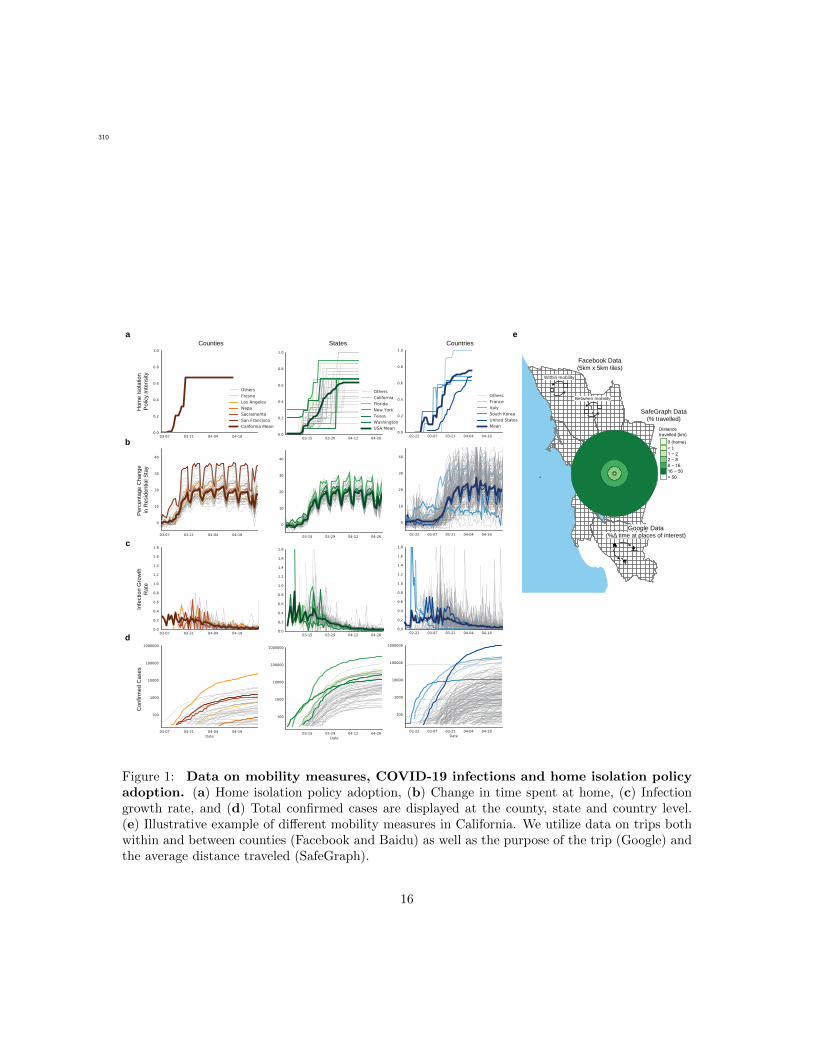
Our study links information on non-pharmaceutical interventions (NPIs, shown in Figure 1a) to68
patterns of human mobility (Figure 1b) and COVID-19 cases (Figure 1c-d). All data were obtained69
from publicly available sources. We provide a brief summary of these data here; full details are70
provided in Appendix A.71
Non-Pharmaceutical Interventions72
We obtain NPI data from two sources. At the sub-national level, we use the NPI dataset compiled73
by Hsiang et al. (2020).1 For each sub-national region in five countries, we observe the fraction of74
the population treated with NPIs in each location on each day. We aggregate 13 different policy75
actions into four general categories: Shelter in Place, Social Distance, School Closure, and Travel76
Ban. At the national level, we compiled data on national lockdown policies from the Organisation for77
Economic Co-operation and Development (OECD) - Country Policy Tracker,2 and crowed-sourced78
information on Wikipedia and COVID-19 Kaggle competitions.379
1 Global Policy Lab, UC Berkeley, http://www.globalpolicy.science/covid19, website accessed on October 20, 2020.2 The Organisation for Economic Co-operation and Development, https://www.oecd.org/coronavirus/en/#country-
tracker, website accessed on April 12, 2020.3 Kaggle, COVID-19 lockdown dates by country, https://www.kaggle.com/jcyzag/covid19-lockdown-dates-by-
country, website accessed on April 12, 2020.
5
Human Mobility80
We source publicly-available data on human mobility from Google, Facebook, Baidu and SafeGraph.81
These private companies provide free aggregated and anonymized information on the movement of82
users of their online platform (Fig 1e). Data from Google indicates the percentage change in the83
amount of time people spend in different types of locations (e.g., residential, retail, and workplace).484
These changes are relative to a baseline defined as the median value, for the corresponding day of85
the week, during Jan 3–Feb 6, 2020. Facebook provides estimates of the number of trips within86
and between square tiles (of resolution up to 360m2) in a region.5 We aggregate these data to show87
trips between and within sub-national units. Baidu provides similar data, indicating movement88
between and within major Chinese cities.6 Lastly, SafeGraph dataset gives us information on89
average distance travelled from home by millions of devices across the US.790
COVID-19 Cases91
For each subnational and national unit, we obtain the cumulative confirmed cases of COVID-19 from92
the data repository compiled by the Johns Hopkins Center for Systems Science and Engineering93
(JHU CSSE COVID-19 Data).894
Linking Data Sets95
The availability of epidemiological, policy, and mobility data varies across subnational units and96
countries included in the analysis. We distinguish between three different levels of aggregation97
for administrative regions - denoted “ADM2” (the smallest unit), “ADM1”, “ADM0.” Our global98
analysis is conducted using ADM0 data. The country-specific analysis is determined by data avail-99
4 Google, COVID-19 Community Mobility Reports, https://www.google.com/covid19/mobility/, website accessedon March 20, 2020.
5 Facebook Disaster Maps: Aggregate Insights for Crisis Response and Recovery,https://research.fb.com/publications/facebook-disaster-maps-aggregate-insights-for-crisis-response-recovery/,website accessed on March 20, 2020.
6 Baidu, Spatio-temporal Big Data Service, https://huiyan.baidu.com, website accessed on March 20, 2020.7 SafeGraph, Social Distancing Metrics, https://docs.safegraph.com/docs/social-distancing-metrics, website ac-
cessed on March 20, 2020.8 COVID-19 Data Repository by the Center for Systems Science and Engineering (CSSE) at Johns Hopkins Uni-
versity, https://github.com/CSSEGISandData/COVID-19, website accessed on March 20, 2020.
6
ability. Results are provided at the prefecture (ADM2) and province level (ADM1) in China; the100
regional (ADM1) level in France; the province (ADM2) and region (ADM1) level in Italy; the101
province (ADM1) level in South Korea; and the county (ADM2) and state (ADM1) level in the102
United States.103
We merge the sub-national NPI, mobility, and epidemiological data based on administrative104
unit and day to form a single longitudinal (panel) data set for each country. We merge the daily105
country-level observations to construct a longitudinal data sets for the portion of the world we106
observe.107
Methods108
Models109
We decompose the impact of an NPI on infections (∆infections∆NPI ) into two components that can be110
modeled separately: the change in behavior associated with the NPI, and the resulting change in111
infections associated with that change in behavior:112
∆infections
∆NPI=
∆behavior
∆NPI× ∆infections
∆behavior. (1)
We construct models to describe each of these two factors. The “behavior model” describes how113
mobility behavior changes in association with the deployment of NPIs (∆behavior∆NPI ). The “infec-114
tion model” describes how infections change in association with changes in mobility behavior115
(∆infections∆behavior ). Both models are “reduced-form” models, commonly used in econometrics, that char-116
acterize the behavior of these variables without explicitly modeling the underlying mechanisms that117
link them (cf., Hsiang et al., 2020). Instead, these models emulate the output one would expect118
from more sophisticated and mechanistically explicit epidemiological models — without requiring119
the underlying processes to be specified. While this reduced-form approach does not provide the120
same epidemiological insight that more detailed models do, they demand less data and fewer as-121
sumptions. For example, they can be fit to local data by analysts with basic statistical training,122
7

not necessarily in epidemiology, and they do not require knowledge of fundamental epidemiological123
parameters — some of which may differ in each context and can be difficult to determine. The124
performance of these simple, low-cost models can then be evaluated via cross-validation, i.e., by125
systematically evaluating out-of-sample forecast quality.126
Behavior Model127
For each country, we separately estimate how daily sub-national mobility behavior changes in128
association with the deployments of NPIs using a country-specific model. In the global model, we129
pool data across countries and estimate how mobility in each country changes in association with130
national exposure to NPIs. Each category of mobility on each day is assumed to be simultaneously131
influenced by the collection of NPIs that are active in that location on that day. A panel multiple132
linear regression model is used to estimate the relative association of each category of mobility133
with each NPI. Our approach accounts for constant differences in baseline mobility between and134
within each sub-national unit – such as differences due to regional commuting patterns, culture,135
or geography, and differences in mobility across days of the week. These effects are not modeled136
explicitly but instead are accounted for non-parametrically. Appendix B.1 contains details of the137
modeling approach.138
Infection Model139
As with the behavior model, we model the daily growth rate of infections at the local, national,140
and global scale. In each location, we model the daily growth rate of infections as a function of141
recent human mobility and historical infections. The approach does not require epidemiological142
parameters, such as the incubation period or R0, nor information on NPIs.143
In practice, we estimate a distributed-lag model where the predictor variables are mobility rates144
in that location for the prior 21 days, and the dependent variable is the daily infection growth145
rate, constructed as the first-difference of log confirmed infections. This approach captures the146
intuition that human mobility is a key factor in determining rates of infection, but does not require147
parametric assumptions about the nature of that dependency. The model also accounts for constant148
8

differences in baseline infection growth rates within each locality — such as those due to differences149
in local behavior unrelated to mobility, differences across days of the week, and changes in how150
confirmed infections are defined or tested for. This approach is also robust to incomplete rates of151
COVID-19 testing, uneven patterns of testing across space, and gradual changes in testing over152
time (Hsiang et al., 2020).153
We fit the model using historical data from each location, and follow stringent practices of154
cross-validation to ensure that the models are not ‘overfit’ to historical trends. The accuracy of155
the forecast is then evaluated against actual infections observed during the forecast period, but156
which were not used to fit the model. Models are fit at the finest administrative level where data157
are available and forecasts are aggregated to larger regions to evaluate the ability of the model158
to predict infections at different spatial scales. Appendix B.2 contains details of the modeling159
approach.160
In principle, such future forecasts can be used by decision-makers who are able to influence local161
mobility through policy and/or NPIs, perhaps informed either by a behavioral model or observation.162
Here, we test the quality of the infection model to generate forecasts by simulating and evaluating163
what a forecaster would have predicted had they generated a forecast at a historical date. In the164
forecasts presented here, we assume that mobility remains at the level observed during the forecast165
period – although in practice we expect that decision-makers would simulate different forecasts166
under different mobility assumptions to inform NPI deployment and policy-making.167
Results168
We first present results from our behavior model, characterizing the mobility response of different169
populations to different NPIs. We then evaluate the infection model’s ability to forecast COVID-19170
infections based on these same mobility measures. We conclude by discussing how these models171
could be used to guide policy decisions at local and regional scales.172
9
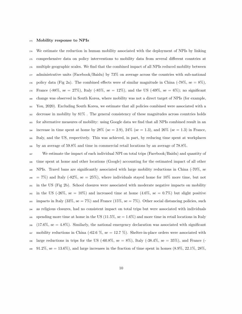
Mobility response to NPIs173
We estimate the reduction in human mobility associated with the deployment of NPIs by linking174
comprehensive data on policy interventions to mobility data from several different countries at175
multiple geographic scales. We find that the combined impact of all NPIs reduced mobility between176
administrative units (Facebook/Baidu) by 73% on average across the countries with sub-national177
policy data (Fig 2a). The combined effects were of similar magnitude in China (-78%, se = 8%),178
France (-88%, se = 27%), Italy (-85%, se = 12%), and the US (-69%, se = 6%); no significant179
change was observed in South Korea, where mobility was not a direct target of NPIs (for example,180
You, 2020). Excluding South Korea, we estimate that all policies combined were associated with a181
decrease in mobility by 81% . The general consistency of these magnitudes across countries holds182
for alternative measures of mobility: using Google data we find that all NPIs combined result in an183
increase in time spent at home by 28% (se = 2.9), 24% (se = 1.3), and 26% (se = 1.3) in France,184
Italy, and the US, respectively. This was achieved, in part, by reducing time spent at workplaces185
by an average of 59.8% and time in commercial retail locations by an average of 78.8%.186
We estimate the impact of each individual NPI on total trips (Facebook/Baidu) and quantity of187
time spent at home and other locations (Google) accounting for the estimated impact of all other188
NPIs. Travel bans are significantly associated with large mobility reductions in China (-70%, se189
= 7%) and Italy (-82%, se = 25%), where individuals stayed home for 10% more time, but not190
in the US (Fig 2b). School closures were associated with moderate negative impacts on mobility191
in the US (-26%, se = 10%) and increased time at home (4.6%, se = 0.7%) but slight positive192
impacts in Italy (33%, se = 7%) and France (15%, se = 7%). Other social distancing policies, such193
as religious closures, had no consistent impact on total trips but were associated with individuals194
spending more time at home in the US (11.5%, se = 1.6%) and more time in retail locations in Italy195
(17.6%, se = 4.8%). Similarly, the national emergency declaration was associated with significant196
mobility reductions in China (-62.6 %, se = 12.7 %). Shelter-in-place orders were associated with197
large reductions in trips for the US (-60.8%, se = 8%), Italy (-38.4%, se = 35%), and France (-198
91.2%, se = 13.6%), and large increases in the fraction of time spent in homes (8.9%, 22.1%, 28%,199
10

respectively). Shelter in place orders did not appear to have large impacts in South Korea or China.200
This is consistent with earlier policies (such as the Emergency Declaration) restricting movement in201
China earlier than the shelter in place orders, while mobility in South Korea was never substantially202
affected by NPIs.203
Globally, we find evidence that lockdown policies were associated with substantial reductions204
in mobility (Figure 2c). Across 80 countries, the average time spend in non-residential locations205
decreased by 40% (se = 2%) in response to NPIs. Time spent in retail locations is the most206
impacted category, declining 49.9% (se = 2%). Some of the variation in response across countries207
(grey dots) likely reflects different social, cultural, and economic norms; measurement error; and208
statistical variability. In Appendix C, we disaggregate this effect temporally, and find that the most209
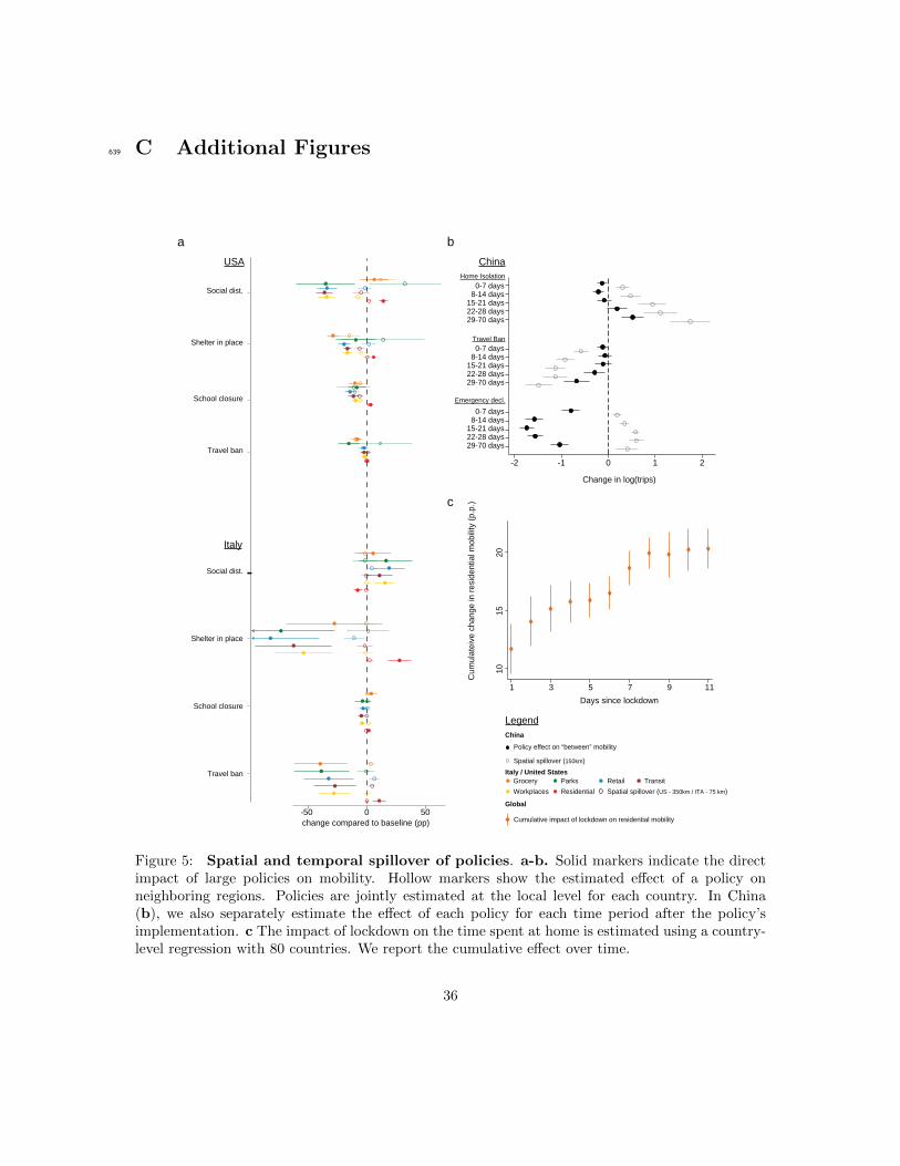
significant reductions occur during the first eight days after a lockdown (Figure 5c).210
In Appendix C, we further exploit the granular resolution of the mobility data to investigate211
whether localized policies also impacted neighboring regions (Figure 5). In the USA and Italy,212
the impact of NPIs on mobility was highly localized, with little evidence of spatial spillover effects213
(Appendix C - Figure 5a). In China, the evidence is more mixed, with some evidence of spillovers214
between neighboring cities (Appendix C - Fig 5b).215
Forecasting infections based on mobility216
We find that mobility data alone are sufficient to meaningfully forecast COVID-19 infections 7-10217
days ahead at all geographic scales – from counties and cities (ADM2), to states and provinces218
(ADM1), to countries (ADM0) and the entire world. Furthermore, identical models that exclude219
mobility data perform substantially worse, suggesting an important role for mobility data in fore-220
casting.221
Figure 3 illustrates the performance of model forecasts in several geographic regions and at222
multiple scales. The true infection rate is shown as a solid line; data used to train each model223
are depicted in blue dots, and the forecast of our model is shown in orange, contrasted against a224
model with no mobility data in green. Forecasts that account for current and lagged measures of225
mobility generally track actual cases more closely than forecasts that do not account for mobility.226
11
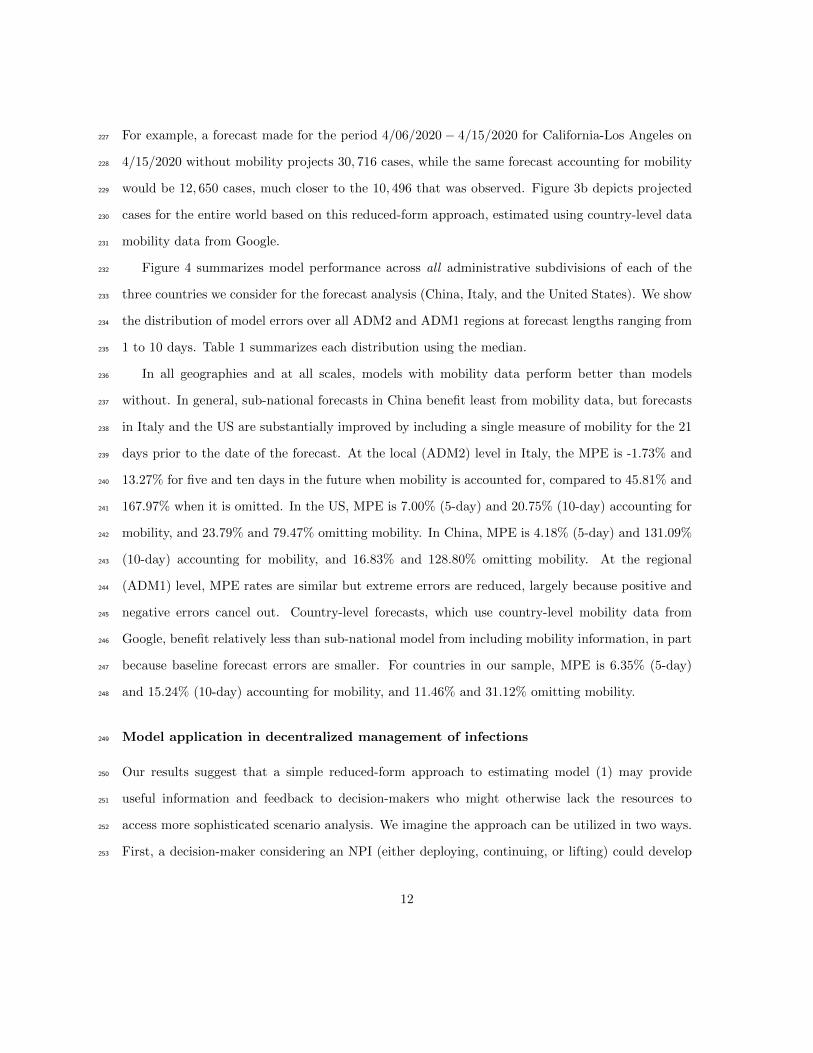
For example, a forecast made for the period 4/06/2020 − 4/15/2020 for California-Los Angeles on227
4/15/2020 without mobility projects 30, 716 cases, while the same forecast accounting for mobility228
would be 12, 650 cases, much closer to the 10, 496 that was observed. Figure 3b depicts projected229
cases for the entire world based on this reduced-form approach, estimated using country-level data230
mobility data from Google.231
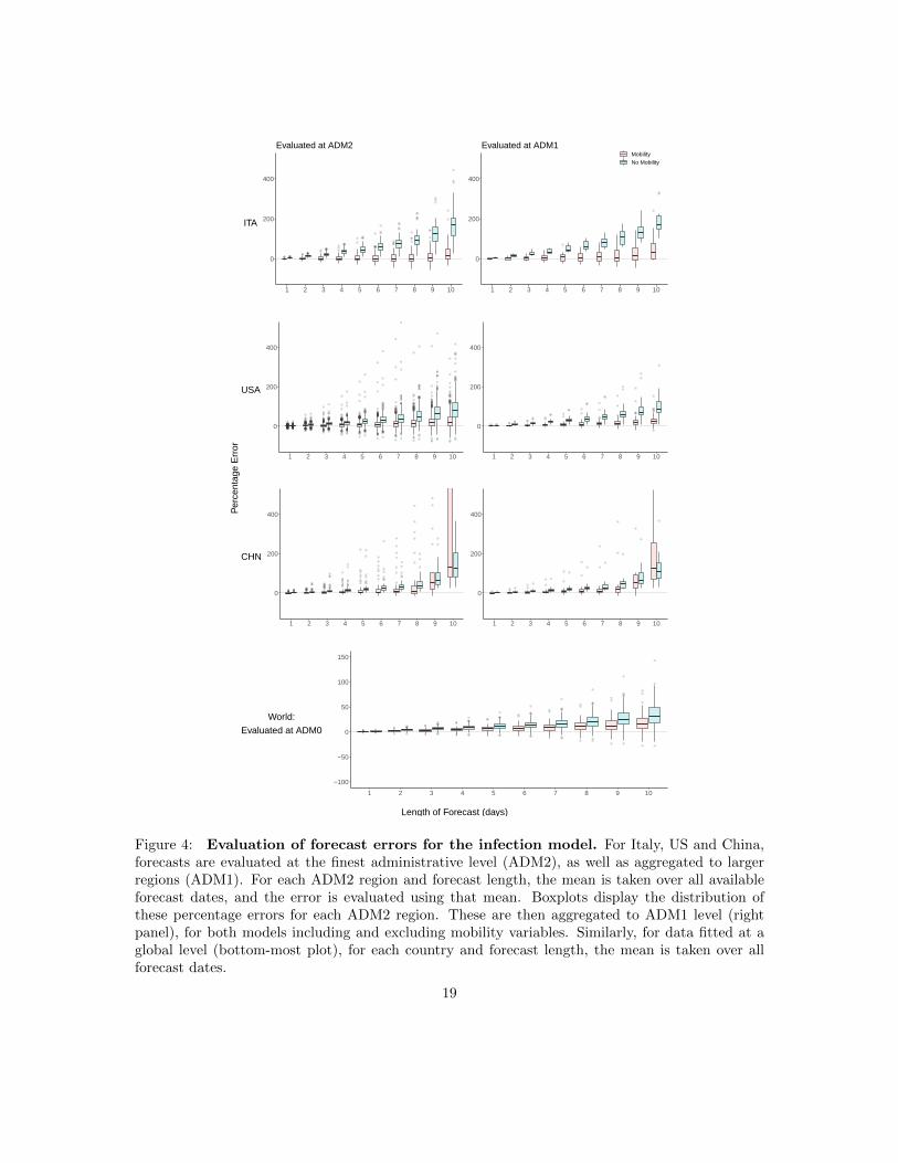
Figure 4 summarizes model performance across all administrative subdivisions of each of the232
three countries we consider for the forecast analysis (China, Italy, and the United States). We show233
the distribution of model errors over all ADM2 and ADM1 regions at forecast lengths ranging from234
1 to 10 days. Table 1 summarizes each distribution using the median.235
In all geographies and at all scales, models with mobility data perform better than models236
without. In general, sub-national forecasts in China benefit least from mobility data, but forecasts237
in Italy and the US are substantially improved by including a single measure of mobility for the 21238
days prior to the date of the forecast. At the local (ADM2) level in Italy, the MPE is -1.73% and239
13.27% for five and ten days in the future when mobility is accounted for, compared to 45.81% and240
167.97% when it is omitted. In the US, MPE is 7.00% (5-day) and 20.75% (10-day) accounting for241
mobility, and 23.79% and 79.47% omitting mobility. In China, MPE is 4.18% (5-day) and 131.09%242
(10-day) accounting for mobility, and 16.83% and 128.80% omitting mobility. At the regional243
(ADM1) level, MPE rates are similar but extreme errors are reduced, largely because positive and244
negative errors cancel out. Country-level forecasts, which use country-level mobility data from245
Google, benefit relatively less than sub-national model from including mobility information, in part246
because baseline forecast errors are smaller. For countries in our sample, MPE is 6.35% (5-day)247
and 15.24% (10-day) accounting for mobility, and 11.46% and 31.12% omitting mobility.248
Model application in decentralized management of infections249
Our results suggest that a simple reduced-form approach to estimating model (1) may provide250
useful information and feedback to decision-makers who might otherwise lack the resources to251
access more sophisticated scenario analysis. We imagine the approach can be utilized in two ways.252
First, a decision-maker considering an NPI (either deploying, continuing, or lifting) could develop253
12

an estimate for how that NPI might affect behavior, based on our analysis of different policies above254
(Fig 2). Using these estimated changes in mobility, they could then forecast changes in infections255
using the infection model described above — but fit to local data.256
Table 2 provides an example calculation for how a novel policy that increased residential time257
(observed in Google data) would alter future infections, using estimates from the global-level model.258
For example, a policy that increases residential time by 5% in a country is predicted to reduce259
cumulative infections ten days later, to 82.5% (CI: (78.2, 87.0)) of what they would otherwise have260
been. Similar tabulations can be generated by fitting infection models using recent and local data,261
which would flexibly capture local social, economic, and epidemiological conditions.262
A second way that a decision-maker could use our approach would be to actually deploy a policy263
without ex ante knowledge of the effect it will have on mobility, instead simply observing mobility264
responses that occur after NPI deployment using these publicly available data sources. Based on265
these observed responses, they could forecast infections using our behavior model.266
Discussion267
The COVID-19 pandemic has led to an unprecedented degree of cooperation and transparency268
within the scientific community, with important new insights rapidly disseminated freely around269
the globe. However, the capacity of different populations to leverage new scientific insights is not270
uniform. In many resource-constrained contexts, critical decisions are not supported by robust271
epidemiological modeling of scenarios. Here we have demonstrated that freely available mobility272
data can be used in simple models to generate practically useful forecasts. The goal is for these273
models to be accessible to a single individual with basic training in regression analysis using standard274
statistical software. The reduced-form model we develop generally performs well when fit to local275
data, except in China where it cannot account for some key factors that contributed to reductions276
in transmission.277
A key insight from our work is that passively observed measures of aggregate mobility are278
useful predictors of growth in COVID-19 cases. However, this does not imply that population279
13
mobility itself is the only fundamental cause of transmission. The measures of mobility we observe280
capture a degree of “mixing” that is occurring within a population, as populations move about their281
local geographic context. This movement is likely correlated with other behaviors and factors that282
contribute to the spread of the virus, such as low rates of mask-wearing and/or physical distancing.283
Our approach does not explicitly capture these other factors — and thus should not be used to284
draw causal inferences — but is possible that our infection model performs well in part because the285
easy-to-observe mobility measures capture these other factors by proxy.286
The simple model we present here is designed to provide useful information in contexts when287
more sophisticated process-based models are unavailable, but it should not necessarily displace288
those models where they are available. In cases where complete process-based epidemiological289
models have been developed for a population and can be deployed for decision-making, the model290
we develop here could be considered complementary to those models. Future work might determine291
how information from combinations of qualitatively distinct models can be used to optimally guide292
decision-making.293
We also note that the reduced-form model is designed to forecast infections in a certain popu-294
lation at a restricted point in time. It achieves this by capturing dynamics that are governed by295
many underlying processes that are unobserved by the modeler. However, because these underlying296
mechanisms are only captured implicitly, the model is not well-suited to environments where these297
underlying dynamics change dramatically. In such circumstances, process-based models will likely298
perform better. Nonetheless, the reduced-form approach presented here can also be applied in these299
circumstances, but it may be necessary to refit the model based on data that is representative of300
current conditions. Similarly, when our reduced-form model is applied to a new population, it301
should be fit to local data to capture dynamics representative of the new population.302
The approach we present here depends critically on the availability of aggregate mobility data,303
which is currently provided to the public by private firms that passively collect this information. We304
hypothesize that the approach we develop here might skillfully forecast the spread of other diseases305
besides COVID-19. If true, this suggests our approach could provide useful information to decision-306
makers for managing other public health challenges, such as influenza or other outbreaks, potentially307
14

indicating a public health benefit from firms continuing to made mobility data available—even after308
the COVID-19 pandemic has subsided.309
15
310
Counties
Hom
e Is
olat
ion
Polic
y In
tens
ityPe
rcen
tage
Cha
nge
in R
esid
entia
l Sta
yIn
fect
ion
Gro
wth
Rat
eC
onfir
med
Cas
es
a
b
c
d
States Countries
Facebook Data(5km x 5km tiles)
e
SafeGraph Data(% travelled)
< 11 − 22 − 88 − 1616 − 50
Distancetravelled (km)
> 50
0 (home)
Between mobility
Within mobility
Google Data(%Δ time at places of interest)
Figure 1: Data on mobility measures, COVID-19 infections and home isolation policyadoption. (a) Home isolation policy adoption, (b) Change in time spent at home, (c) Infectiongrowth rate, and (d) Total confirmed cases are displayed at the county, state and country level.(e) Illustrative example of different mobility measures in California. We utilize data on trips bothwithin and between counties (Facebook and Baidu) as well as the purpose of the trip (Google) andthe average distance traveled (SafeGraph).
16

-3 -2 -1 0 1change in log(trips)
Other social distance
Emergency Declaration
Shelter-in-place
School closure
Travel ban
Combined effect
change compared to baseline (pp)
a
b
Legend
Effect of lockdown on mobility:Pooled estimate (80 countries)Country level estimate
FranceItaly
South KoreaChinaUSA
Policy impact by type of mobility and country:Mobility between admin. unit
Workplaces related mobility
Residential areas mobilityRetail related mobility Google data
Facebook or Baidu data
South KoreaUSA
ItalyFrance
China
c
Facebook/Baidu data Google data
-100 -50 0 50
Workplaces
Transit
Retail
Residential area
Parks
Grocery & Pharmacy
Time spent:
Figure 2: Empirical estimates of the effect of NPIs on mobility measures. Markers arecountry specific-estimates, whiskers show the 95% confidence interval. a Estimated combined effectof all policies on number of trips between counties (left) and time spent in specific places (right). bEstimated effects of individual policy or policy groups on mobility measures, jointly estimated foreach country. c Estimated effect of lockdown on mobility the 80 countries which experienced suchpolicy, jointly estimated for each type of mobility.17
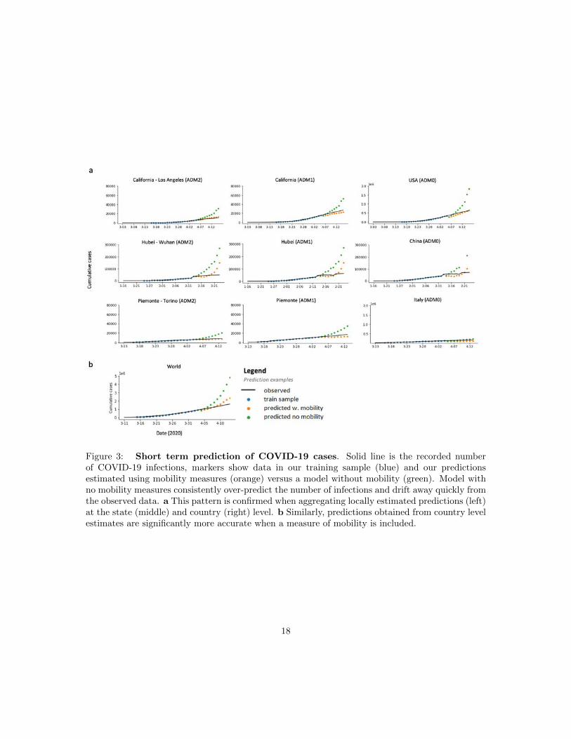
Figure 3: Short term prediction of COVID-19 cases. Solid line is the recorded numberof COVID-19 infections, markers show data in our training sample (blue) and our predictionsestimated using mobility measures (orange) versus a model without mobility (green). Model withno mobility measures consistently over-predict the number of infections and drift away quickly fromthe observed data. a This pattern is confirmed when aggregating locally estimated predictions (left)at the state (middle) and country (right) level. b Similarly, predictions obtained from country levelestimates are significantly more accurate when a measure of mobility is included.
18
0
200
400
1 2 3 4 5 6 7 8 9 10
Evaluated at ADM2
0
200
400
1 2 3 4 5 6 7 8 9 10
MobilityNo Mobility
Evaluated at ADM1
ITA
0
200
400
1 2 3 4 5 6 7 8 9 10
0
200
400
1 2 3 4 5 6 7 8 9 10
USA
0
200
400
1 2 3 4 5 6 7 8 9 10
0
200
400
1 2 3 4 5 6 7 8 9 10
CHN
−100
−50
0
50
100
150
1 2 3 4 5 6 7 8 9 10
World:Evaluated at ADM0
Length of Forecast (days)
Per
cent
age
Err
or
Figure 4: Evaluation of forecast errors for the infection model. For Italy, US and China,forecasts are evaluated at the finest administrative level (ADM2), as well as aggregated to largerregions (ADM1). For each ADM2 region and forecast length, the mean is taken over all availableforecast dates, and the error is evaluated using that mean. Boxplots display the distribution ofthese percentage errors for each ADM2 region. These are then aggregated to ADM1 level (rightpanel), for both models including and excluding mobility variables. Similarly, for data fitted at aglobal level (bottom-most plot), for each country and forecast length, the mean is taken over allforecast dates.
19
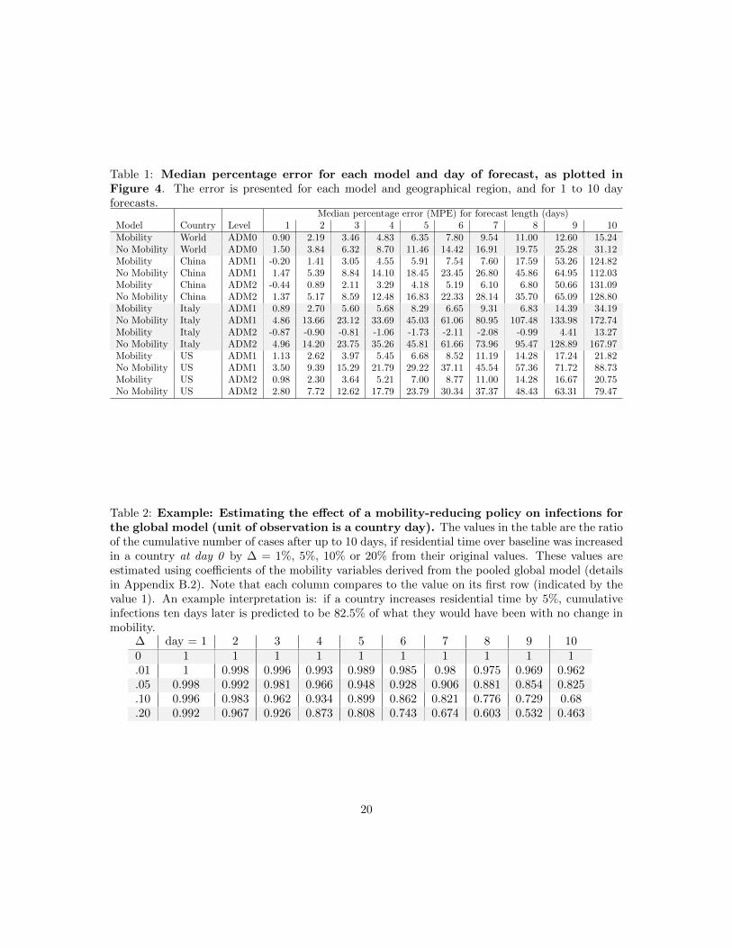
Table 1: Median percentage error for each model and day of forecast, as plotted inFigure 4. The error is presented for each model and geographical region, and for 1 to 10 dayforecasts.
Median percentage error (MPE) for forecast length (days)Model Country Level 1 2 3 4 5 6 7 8 9 10Mobility World ADM0 0.90 2.19 3.46 4.83 6.35 7.80 9.54 11.00 12.60 15.24No Mobility World ADM0 1.50 3.84 6.32 8.70 11.46 14.42 16.91 19.75 25.28 31.12Mobility China ADM1 -0.20 1.41 3.05 4.55 5.91 7.54 7.60 17.59 53.26 124.82No Mobility China ADM1 1.47 5.39 8.84 14.10 18.45 23.45 26.80 45.86 64.95 112.03Mobility China ADM2 -0.44 0.89 2.11 3.29 4.18 5.19 6.10 6.80 50.66 131.09No Mobility China ADM2 1.37 5.17 8.59 12.48 16.83 22.33 28.14 35.70 65.09 128.80Mobility Italy ADM1 0.89 2.70 5.60 5.68 8.29 6.65 9.31 6.83 14.39 34.19No Mobility Italy ADM1 4.86 13.66 23.12 33.69 45.03 61.06 80.95 107.48 133.98 172.74Mobility Italy ADM2 -0.87 -0.90 -0.81 -1.06 -1.73 -2.11 -2.08 -0.99 4.41 13.27No Mobility Italy ADM2 4.96 14.20 23.75 35.26 45.81 61.66 73.96 95.47 128.89 167.97Mobility US ADM1 1.13 2.62 3.97 5.45 6.68 8.52 11.19 14.28 17.24 21.82No Mobility US ADM1 3.50 9.39 15.29 21.79 29.22 37.11 45.54 57.36 71.72 88.73Mobility US ADM2 0.98 2.30 3.64 5.21 7.00 8.77 11.00 14.28 16.67 20.75No Mobility US ADM2 2.80 7.72 12.62 17.79 23.79 30.34 37.37 48.43 63.31 79.47
Table 2: Example: Estimating the effect of a mobility-reducing policy on infections forthe global model (unit of observation is a country day). The values in the table are the ratioof the cumulative number of cases after up to 10 days, if residential time over baseline was increasedin a country at day 0 by ∆ = 1%, 5%, 10% or 20% from their original values. These values areestimated using coefficients of the mobility variables derived from the pooled global model (detailsin Appendix B.2). Note that each column compares to the value on its first row (indicated by thevalue 1). An example interpretation is: if a country increases residential time by 5%, cumulativeinfections ten days later is predicted to be 82.5% of what they would have been with no change inmobility.
∆ day = 1 2 3 4 5 6 7 8 9 100 1 1 1 1 1 1 1 1 1 1.01 1 0.998 0.996 0.993 0.989 0.985 0.98 0.975 0.969 0.962.05 0.998 0.992 0.981 0.966 0.948 0.928 0.906 0.881 0.854 0.825.10 0.996 0.983 0.962 0.934 0.899 0.862 0.821 0.776 0.729 0.68.20 0.992 0.967 0.926 0.873 0.808 0.743 0.674 0.603 0.532 0.463
20

References311
Atkeson, Andrew. 2020. “What will be the economic impact of covid-19 in the us? rough312
estimates of disease scenarios.” National Bureau of Economic Research.313
Cheng, Cindy, Joan Barcelo, Allison Spencer Hartnett, Robert Kubinec, and Luca314
Messerschmidt. 2020. “COVID-19 Government Response Event Dataset (CoronaNet v. 1.0).”315
Nature human behaviour, 4(7): 756–768.316
China-Data-Lab. 2020. “Baidu Mobility Data.” Harvard Dataverse.317
Chinazzi, Matteo, Jessica T Davis, Marco Ajelli, Corrado Gioannini, Maria Litvinova,318
Stefano Merler, Ana Pastore y Piontti, Kunpeng Mu, Luca Rossi, Kaiyuan Sun, et al.319
2020. “The effect of travel restrictions on the spread of the 2019 novel coronavirus (COVID-19)320
outbreak.” Science, 368(6489): 395–400.321
Coibion, Olivier, Yuriy Gorodnichenko, and Michael Weber. 2020. “The cost of the covid-322
19 crisis: Lockdowns, macroeconomic expectations, and consumer spending.” National Bureau323
of Economic Research.324
Engle, Samuel, John Stromme, and Anson Zhou. 2020. “Staying at home: mobility effects325
of covid-19.” Available at SSRN.326
Evans, Michelle V, Andres Garchitorena, Rado JL Rakotonanahary, John M Drake,327
Benjamin Andriamihaja, Elinambinina Rajaonarifara, Calistus N Ngonghala, Ben-328
jamin Roche, Matthew H Bonds, and Julio Rakotonirina. 2020. “Reconciling model329
predictions with low reported cases of COVID-19 in Sub-Saharan Africa: Insights from Mada-330
gascar.” Global Health Action, 13(1): 1816044.331
Ferguson, Neil, Daniel Laydon, Gemma Nedjati Gilani, Natsuko Imai, Kylie Ainslie,332
Marc Baguelin, Sangeeta Bhatia, Adhiratha Boonyasiri, ZULMA Cucunuba Perez,333
Gina Cuomo-Dannenburg, et al. 2020. “Report 9: Impact of non-pharmaceutical interven-334
tions (NPIs) to reduce COVID19 mortality and healthcare demand.”335
Friedman, Joseph, Patrick Liu, Emmanuela Gakidou, IHME COVID, and Model Com-336
parison Team. 2020. “Predictive performance of international COVID-19 mortality forecasting337
models.” medRxiv.338
Gnanvi, Janyce E, Brezesky Kotanmi, et al. 2020. “On the reliability of predictions on339
Covid-19 dynamics: a systematic and critical review of modelling techniques.” medRxiv.340
Gossling, Stefan, Daniel Scott, and C. Michael Hall. 2020. “Pandemics, tourism and global341
change: a rapid assessment of COVID-19.” Journal of Sustainable Tourism, 0(0): 1–20.342
Hsiang, Solomon, Daniel Allen, Sebastien Annan-Phan, Kendon Bell, Ian Bolliger,343
Trinetta Chong, Hannah Druckenmiller, Luna Yue Huang, Andrew Hultgren, Emma344
Krasovich, et al. 2020. “The effect of large-scale anti-contagion policies on the COVID-19345
pandemic.” Nature, 1–9.346
21

Klein, Brennan, T LaRocky, S McCabey, L Torresy, Filippo Privitera, Brennan Lake,347
Moritz UG Kraemer, John S Brownstein, David Lazer, Tina Eliassi-Rad, et al. 2020.348
“Assessing changes in commuting and individual mobility in major metropolitan areas in the349
United States during the COVID-19 outbreak.”350
Kraemer, Moritz U. G., Chia-Hung Yang, Bernardo Gutierrez, Chieh-Hsi Wu,351
Brennan Klein, David M. Pigott, Open COVID-19 Data Working Group†, Louis352
du Plessis, Nuno R. Faria, Ruoran Li, William P. Hanage, John S. Brownstein,353
Maylis Layan, Alessandro Vespignani, Huaiyu Tian, Christopher Dye, Oliver G. Py-354
bus, and Samuel V. Scarpino. 2020. “The effect of human mobility and control measures on355
the COVID-19 epidemic in China.” Science, eabb4218.356
Liverani, Marco, Benjamin Hawkins, and Justin O Parkhurst. 2013. “Political and insti-357
tutional influences on the use of evidence in public health policy. A systematic review.” PloS one,358
8(10): e77404.359
Loembe, Marguerite Massinga, Akhona Tshangela, Stephanie J Salyer, Jay K Varma,360
Ahmed E Ogwell Ouma, and John N Nkengasong. 2020. “COVID-19 in Africa: the spread361
and response.” Nature Medicine, 1–4.362
Martın-Calvo, David, Alberto Aleta, Alex Pentland, Yamir Moreno, and Esteban363
Moro. 2020. “Effectiveness of social distancing strategies for protecting a community from a364
pandemic with a data driven contact network based on census and real-world mobility data.” In365
Technical Report.366
Morita, Hiroyoshi, Hirokazu Kato, and Yoshitsugu Hayashi. 2020. “International compar-367
ison of behavior changes with social distancing policies in response to COVID-19.” Available at368
SSRN 3594035.369
Mueller, Valerie, Glenn Sheriff, Corinna Keeler, and Megan Jehn. 2020. “COVID-19370
Policy Modeling in Sub-Saharan Africa.” Applied Economic Perspectives and Policy.371
Pepe, Emanuele, Paolo Bajardi, Laetitia Gauvin, Filippo Privitera, Brennan Lake,372
Ciro Cattuto, and Michele Tizzoni. 2020. “COVID-19 outbreak response: a first assessment373
of mobility changes in Italy following national lockdown.” medRxiv.374
Ray, Evan L, Nutcha Wattanachit, Jarad Niemi, Abdul Hannan Kanji, Katie House,375
Estee Y Cramer, Johannes Bracher, Andrew Zheng, Teresa K Yamana, Xinyue376
Xiong, et al. 2020. “Ensemble Forecasts of Coronavirus Disease 2019 (COVID-19) in the US.”377
medRxiv.378
Rossi, Rodolfo, Valentina Socci, Dalila Talevi, Sonia Mensi, Cinzia Niolu, Francesca379
Pacitti, Antinisca Di Marco, Alessandro Rossi, Alberto Siracusano, and Giorgio380
Di Lorenzo. 2020. “COVID-19 pandemic and lockdown measures impact on mental health381
among the general population in Italy.” Frontiers in Psychiatry, 11: 790.382
Thunstrom, Linda, Stephen C Newbold, David Finnoff, Madison Ashworth, and Ja-383
son F Shogren. 2020. “The benefits and costs of using social distancing to flatten the curve for384
COVID-19.” Journal of Benefit-Cost Analysis, 1–27.385
22
Tian, Huaiyu, Yonghong Liu, Yidan Li, Chieh-Hsi Wu, Bin Chen, Moritz UG Krae-386
mer, Bingying Li, Jun Cai, Bo Xu, Qiqi Yang, et al. 2020. “An investigation of trans-387
mission control measures during the first 50 days of the COVID-19 epidemic in China.” Science,388
368(6491): 638–642.389
Twahirwa Rwema, Jean Olivier, Daouda Diouf, Nancy Phaswana-Mafuya,390
Jean Christophe Rusatira, Alain Manouan, Emelyne Uwizeye, Fatou M Drame,391
Ubald Tamoufe, and Stefan David Baral. 2020. “COVID-19 Across Africa: Epidemiologic392
Heterogeneity and Necessity of Contextually Relevant Transmission Models and Intervention393
Strategies.”394
Wellenius, Gregory A, Swapnil Vispute, Valeria Espinosa, Alex Fabrikant, Thomas C395
Tsai, Jonathan Hennessy, Brian Williams, Krishna Gadepalli, Adam Boulange,396
Adam Pearce, et al. 2020. “Impacts of state-level policies on social distancing in the397
united states using aggregated mobility data during the covid-19 pandemic.” arXiv preprint398
arXiv:2004.10172.399
You, Jongeun. 2020. “Lessons from South Korea’s Covid-19 policy response.” The American400
Review of Public Administration, 50(6-7): 801–808.401
23

Acknowledgements: We thank Jeanette Tseng for her role in designing Fig. 1. S.A.P. is sup-402
ported by a gift from the Tuaropaki Trust. This material is based upon work supported by the403
National Science Foundation under Grant IIS-1942702. Any opinions, findings, and conclusions404
or recommendations expressed in this material are those of the authors and do not necessarily405
reflect the views of the National Science Foundation. Funding was also provided by Award 2020-406
0000000149 from CITRIS and the Banatao Institute at the University of California. None of the407
authors has been paid to write this article by a pharmaceutical company or other agency. All authors408
had full access to the full data in the study and accept responsibility to submit for publication.409
Author contributions: J.B. and S.H. conceived and led the study. C.I., J.B., S.A.P., S.H., X.H.T.,410
designed analysis, and interpreted results. C.I., S.A.P., S.M., and X.H.T. collected, verified, cleaned411
and merged data. C.I. created Figs. 3, 6 and Table 3. S.A.P. created Figs. 2, 5. S.M. created412
Fig. 1 and Table 6. X.H.T. created Fig.4 and Tables 1,2. X.H.T. managed literature review. All413
authors wrote the paper. C.I., S.A.P., and X.H.T. contributed equally and are listed in a randomly414
assigned order.415
Role of funding source: S.A.P. is supported by a gift from the Tuaropaki Trust. This material416
is based upon work supported by the National Science Foundation under Grant IIS-1942702, the417
Office of Naval Research (Minerva Initiative) under award N00014-17-1-2313, and CITRIS and the418
Banatao Institute at the University of California under Award 2020-0000000149. Any opinions,419
findings, and conclusions or recommendations expressed in this material are those of the authors420
and do not necessarily reflect the views of the National Science Foundation, the Office of Naval421
Research, or any other funding institution.422
Declaration of interests: The authors declare no competing interests.423
24

Appendices424
A Data Acquisition and Processing425
Data used in this study can be divided into three categories - Epidemiological, Policy and Mobil-426
ity. The sources of these data sets include various research institutions, government public health427
websites, regional newspaper articles and digital social media platforms.428
A.1 Epidemiological Data429
We collected epidemiological data from the 2019 Novel Coronavirus COVID-19 (2019-nCoV) Data430
Repository compiled by the Johns Hopkins Center for Systems Science and Engineering (JHU431
CSSE).9 The primary variable of interest for our study is cum confirmed cases, i.e., the total number432
of confirmed positive cases in an administrative area since the first confirmed case. We accessed it433
along with other relevant metadata, including:434
date: The date of observation435
adm0 name: The ISO3 region (Administrative Level 0) code of the observation436
adm1 name: The name of the “Administrative Level 1” region of the observation437
adm2 name: The name of the “Administrative Level 2” region of the observation438
A.2 Policy data439
The policy data was constructed and made available for academic research by Hsiang et al. (2020).10440
For each country, the relevant country-specific policies were identified and mapped to four harmo-441
nized policy categories - Travel Ban, School Closure, Shelter in place, and Social Distance. These442
category variables were created by taking an average of policy variables related to that category.443
i. Travel Ban444
9 https://github.com/CSSEGISandData/COVID-1910 http://www.globalpolicy.science/covid19
25
• travel ban local : Represents a policy that restricts people from entering or exiting the445
administrative area (e.g., county or province) treated by the policy.446
ii. School Closure447
• school closure: Represents a policy that closes school and other educational services in448
that area.449
iii. Shelter In Place450
• home isolation: Represents a policy that prohibits people from leaving their home re-451
gardless of their testing status. For some countries, the policy can also include the case452
when people have to stay at home, but are allowed to leave for work- or health-related453
purposes. For the latter case, when the policy is moderate, this is coded as home isolation454
= 0.5.455
• work from home : Represents a policy that requires people to work remotely. This policy456
may also include encouraging workers to take holiday/paid time off.457
• business closure : Represents a policy that closes all offices, non-essential businesses, and458
non-essential commercial activities in that area.459
• pos cases quarantine : A policy that mandates that people who have tested positive for460
COVID-19, or subject to quarantine measures, have to confine themselves at home. The461
policy can also include encouraging people who have fevers or respiratory symptoms to462
stay at home, regardless of whether they tested positive or not.463
• welfare service closure: A policy that mandates closure of welfare services such as day464
care centers for children.465
• emergency declaration: Represents a decision made at the city / municipality, county,466
state / provincial, or federal level to declare a state of emergency. This allows the affected467
area to marshal emergency funds and resources as well as activate emergency legislation.468
iv. Social Distance469
26

• social distance: Represents a policy that encourages people to maintain a safety distance470
(often between one to two meters) from others. This policy differs by country, but471
includes other policies that close cultural institutions (e.g., museums or libraries), or472
encourage establishments to reduce density, such as limiting restaurant hours.473
• no gathering : Represents a policy that prohibits any type of public or private gathering.474
(whether cultural, sporting, recreational, or religious). Depending on the country, the475
policy can prohibit a gathering above a certain size, in which case the number of people476
is specified by the no gathering size variable.477
• event cancel : Represents a policy that cancels a specific pre-scheduled large event (e.g.,478
parade, sporting event, etc). This is different from prohibiting all events over a certain479
size.480
• religious closure: Represents a policy that prohibits gatherings at a place of worship,481
specifically targeting locations that are epicenters of COVID-19 outbreak. See the section482
on Korean policy for more information on this policy variable.483
• no demonstration: Represents a policy that prohibits protest-specific gatherings. See484
the section on Korean policy for more information on this policy variable.485
A.3 Mobility data486
Mobility data comes from three of the biggest internet companies - Google, Facebook and Baidu.487
These companies have millions of users accessing their social media, e-commerce and other digital488
platforms every day. These data are utilized to construct aggregated, anonymized user location and489
movement metrics for various geographic regions and countries. Descriptions follow, and Table 3490
contains a summary of the data used for each country.491
27
A.3.1 Google492
Google mobility data summarizes time spent by their users each day after Feb 6, 2020 in various493
types of places, such as residential, workplaces and grocery stores.11 Specifically, it provides the494
percentage change in number of visits and length of stay in each type of place, compared to a495
baseline value. The baseline is the value on the corresponding day of the week during the 5-week496
period between Jan 3, 2020 and Feb 6, 2020. The metrics are available starting Feb 15, 2020 at the497
country (Administrative Level 0) and state level (Administrative Level 1) for over 135 countries.498
We also access county-level metrics (Administrative Level 2) for the US. Types of places include499
the following:500
i. Grocery & pharmacy : Places like grocery markets, food warehouses, farmers markets, spe-501
cialty food shops, drug stores, and pharmacies.502
ii. Parks: Places like local parks, national parks, public beaches, marinas, dog parks, plazas,503
and public gardens.504
iii. Transit stations: Places like public transport hubs such as subway, bus, and train stations.505
iv. Retail & recreation: Places like restaurants, cafes, shopping centers, theme parks, museums,506
libraries, and movie theaters.507
v. Residential : Places of residence.508
vi. Workplaces: Places of work.509
A.3.2 Facebook510
Facebook summarizes and anonymizes its user data into useful metrics that can be used to evaluate511
the movement of people.12,13 Our analysis uses data beginning March 5, Feb 23 and Feb 24, 2020512
for France, Italy and South Korea respectively. Specifically, Facebook aggregates the number of513
11 https://www.google.com/covid19/mobility/12 https://research.fb.com/publications/facebook-disaster-maps-aggregate-insights-for-crisis-response-recovery/13 https://about.fb.com/news/2017/06/using-data-to-help-communities-recover-and-rebuild/
28
trips between tiles of up to a resolution of 360 square meters. We aggregate these data to the level514
of administrative regions, constructing metrics for number of trips between as well as within these515
regions. We use the following variables from the data provided by Facebook:516
i. Date - The day of the movement.517
ii. Starting Location - The region or tile where the movement of the group started.518
iii. Ending Location - The region or tile where the movement of the group ended.519
iv. Baseline Movement - The total number of people who moved from Starting Location to520
Ending Location on average during the weeks before the disaster began.521
v. Crisis Movement - The total number of people who moved from Starting Location to Ending522
Location during the time period specified523
A.3.3 Baidu524
Baidu provides aggregated user location data and mobility metrics via its Smart Eye Platform.14525
These data were scraped and publicly shared by the China Data Lab. The metrics represent526
movement in and out of major regions across China each day in terms of an aggregated mobility527
index (China-Data-Lab, 2020). Index values are available beginning Jan 1, 2020. Baidu does not528
disclose specific information regarding the construction of the index.529
A.3.4 SafeGraph530
SafeGraph data were generated by tracking anonymous mobile devices across US.15 The mobility531
metrics are available starting January 1, 2020 for census block group. SafeGraph infers home532
location based on night time location of the device and uses that to impute average distance533
travelled per day by the devices in each census block. We aggregate this data to the state level534
(Administrative Level 1) for our analysis.535
14 https://huiyan.baidu.com15 https://docs.safegraph.com/docs/social-distancing-metrics
29

Table 3: Mobility Data Sources - Details of mobility data sources for each country. The tableprovides relevant dates and level of analysis used for the behavior model and infection model,respectively.
Region Mobility Data Level of analysis Type of mobility Start Date End Date
Behavior model
China Baidu ADM2 between 1/10/2020 3/6/2020
France Facebook ADM1 between 3/4/2020 4/8/2020
Italy Facebook ADM2 between 2/25/2020 4/8/2020
South Korea Facebook ADM2 between 2/23/2020 4/6/2020
United States Google ADM2 residential, 3/3/2020 4/12/2020retail,workplaces
World Google ADM0 residential, 2/26/2020 3/28/2020retail,workplaces
Infection model
China Baidu ADM1, ADM2 between 2/12/2020 3/3/2020
France Facebook - - - -
Italy Facebook ADM1, ADM2 between 3/31/2020 4/13/2020
South Korea Facebook - - - -
United States Google ADM1, ADM2 - 3/17/2020 4/30/3020
World Google ADM0 - mobility today >= 5% 5/29/2020or until growth rates
of new cases flatten
30

B Methods Summary536
B.1 Behavior Model537
The behavior model describes how human mobility changes as a result of NPIs (∆behavior∆NPI in equation538
(1)). The model is a commonly used reduced-form approach in econometrics. Details on the model539
and model estimation are presented below.540
Model details:541
1. The model used for each policy is mt = f(policyt, Xt) + εt, where mt is a measure of mobility542
behavior at time t, Xt represents control variables, and εt is the error.543
2. The model is fit for each country at the sub-national level where granular policy and mobility544
data are available. For the rest of the world, use a panel regression model where the unit of545
observation is at the country by day level.546
3. The policy variable is a vector with NPIs specific to each country, for each location and day.547
NPIs are continuous variables between 0 and 1 (inclusive) that indicate the intensity of the548
policy where 0 is no enforcement and 1 is fully enacted. In some instances, it may be desirable549
to gather multiple policies in a single variable (for example, business closure and restaurant550
closure) by taking the average, thus the maximum value of 1 would indicate that all policies551
are fully enacted.552
4. The control variable X includes one-hot encodings of sub-national (or national) units and553
day-of-week variables. The former account for time-invariant factors (for example, socio-554
economic status, culture, public transportation availability) that impact mobility m, while555
the later control for weekly patterns in mobility (for example, less workplace related mobility556
on Sunday) that are common across location unit.557
Steps for model estimation:558
1. Estimate the average effect on mobility in all subsequent periods, β, of each policy included559
in each model using the model described above, and ordinary least squares.560
31

2. Compute the combined effect of policies on human mobility by taking the sum across all β.561
B.2 Infection Model562
Similar to the behavior model, the infection model is also a reduced-form approach, used to describe563
the relationship between infections and mobility behavior (∆infections∆behavior in equation (1)). Model564
details, as well as steps for model estimation, forecasting and cross-validation are outlined below.565
Also included are steps for data selection.566
Model details:567
1. The model used is log( ItIt−1
) = g(mobilityt, Xt) + εt, where log( ItIt−1
) is the first-difference of568
log confirmed infections at time t, Xt represents control variables, and εt is the error.569
2. The model is fit for each country at the sub-national level where granular infections and570
mobility data are available. For the global model, use a regression model where the unit of571
observation is at the country by day level.572
3. The mobility variable is a vector with mobility rates specific to each country, for each location573
and day. Includes mobility measures averaged over lags 1-7, 8-14 and 15-21, respectively.574
We use Google mobility data in its original form (percentage points), and take logs for the575
Facebook and Baidu mobility data.576
4. The control variable X includes one-hot encodings of sub-national (or national) units and577
day-of-week variables.578
Steps for model estimation: The following steps are used to generate estimates of the average579
effect of each mobility variable on the growth rate of infections (see Figure 6). These are then used580
to estimate how a novel policy affecting mobility would alter future infections (Table 2).581
1. Estimate the average effect of each mobility variable on the growth rate of infections, βββ, using582
the model described above, and ordinary least squares.583
32
2. To estimate the potential effect of a mobility-reducing policy, use ∆I = h(∆m, βββ), where ∆I584
is the change in number of infections, ∆m is the anticipated change in mobility due to NPIs,585
and βββ are estimated coefficients of the mobility variables.586
3. Specifically, for Facebook and Baidu data, where mobility variables are in log form: at forecast587
day k, Inew
Ioriginal= ek(
∑3l=1 βl log(1+∆ml)), where ∆ml is the fractional change in the lth mobility588
variable (number of trips for all lags involved) (e.g., if the number of trips for all lags in589
the lth variable is reduced by 10%, ∆ml = −.1). For Google data: at forecast day k,590
Inew
Ioriginal= ek(
∑3l=1 βl∆l), where ∆ml is the change in residential time over baseline for the lth591
mobility variable (e.g., ∆ml = .05 means a 5% increase, say from 20% to 25% residential time592
over baseline, for all lags in the lth variable).593
Steps for forecasting and cross-validation:594
1. For a 20-day period (training data), fit a regression model as specified above, using ordinary595
least squares.596
2. For a 10-day period (test data), multiply the coefficient estimates obtained from fitting the597
regression model on the training data with the observed predictor variables in the test data598
to obtain prediction of the infection rate.599
3. For each test day, compute the percentage error compared to the ground-truth infection rate.600
4. Perform cross-validation (i.e., robustness to train and test sample selection), for all 20-day601
training periods and 10-day forecast periods, limited by data availability.602
5. Group percentage errors by day of forecast (from 1 to 10).603
6. Repeat the above, using a baseline model which excludes mobility variables, i.e., log( ItIt−1
) =604
j(Xt) + εt.605
In other words, the baseline model simply uses past infections to predict future infections. Smaller606
errors using the model including mobility variables would indicate that information on mobility607
improves forecasts. Examples of the results are in Figure 3, and forecasting errors are in 4.608
33

Steps for data selection:609
The time period that we consider (see Table 3) is the “first wave” of infections, and to demon-610
strate the utility of the mobility model, we focus on the period in which mobility starts falling611
as a result of lockdown measures imposed during this first wave, until right before mobility starts612
increasing again. This model can be refit to the local context of interest, using data that is represen-613
tative of current conditions. For countries in which lockdown policy data are available, we include614
administrative regions after the lockdown policy has been implemented. For countries without pol-615
icy data available on a granular enough level (US in this case), we use a start date of March 17 (the616
results are robust to different start dates), or when Google residential mobility is at least 5 percent617
above baseline (world level). We select an end date that roughly corresponds to just before mobility618
picks back up. The reason for this choice is that in the phase in which mobility starts to increase,619
we might expect there to be other measures put in place, or other changes in behavior, such as620
contact tracing, mask wearing, and so forth, which justified the lifting of lockdown measures and621
subsequent increase in mobility. The relationship between mobility and cases might therefore be622
different than during the lockdown stage, suggesting that the model needs to be refit if we would623
like for it to be used during this period.624
Now, we train each model using 20 days of training data, and forecast for up to 10 days into the625
future. To be included in the data used to train each model, we impose the following conditions626
at the level of the administrative region. For the administrative region to be included, for all 20627
training days t,628
1. It ≥ 10629
2. It−1 > 0630
and for the world-level analysis only:631
3. mobilityt ≥ 5 percent, i.e., current day mobility is at least 5 percent above baseline.632
4.(
log ItIt−1
)i,1−14
≤ .03 percent, i.e., the 14 days rolling average of the growth rate of cumulative633
active cases flattens.634
34

These conditions also imply that It, It−1 and the mobility variables have to be non-missing for635
all training days. These conditions have implications for predictions as well: if an administrative636
region is not included in the training data, predictions will not be generated for that region, because637
the region fixed effect would not be estimated for that region.638
35
C Additional Figures639
Policy effect on “between” mobility
Spatial spillover (150km)
Travel ban
School closure
Shelter in place
Social dist.
a b
c
USA
Grocery Parks Retail TransitWorkplaces
Cumulative impact of lockdown on residential mobility
Residential Spatial spillover (US - 350km / ITA - 75 km)
Home Isolation
Travel Ban
Emergency decl.
China
-50 0 50
Travel ban
School closure
Shelter in place
Social dist.
1015
20
1 3 5 7 9 11Days since lockdown
Change in log(trips)
change compared to baseline (pp)
LegendChina
Italy / United States
Global
Cum
ulat
eive
cha
nge
in re
side
ntia
l mob
ility
(p.p
.)
Italy
0-7 days8-14 days
22-28 days29-70 days
-2 -1 0 1 2
15-21 days
0-7 days8-14 days
22-28 days29-70 days
15-21 days
0-7 days8-14 days
22-28 days29-70 days
15-21 days
Figure 5: Spatial and temporal spillover of policies. a-b. Solid markers indicate the directimpact of large policies on mobility. Hollow markers show the estimated effect of a policy onneighboring regions. Policies are jointly estimated at the local level for each country. In China(b), we also separately estimate the effect of each policy for each time period after the policy’simplementation. c The impact of lockdown on the time spent at home is estimated using a country-level regression with 80 countries. We report the cumulative effect over time.
36

Figure 6: Impact of mobility on the growth rate of COVID-19 cases. Estimated impactof mobility on COVID-19 infection growth rate over time. Effects are estimated for each of thepreceding three weeks (lags of 1 to 21 days), where the measure of mobility is either the number oftrips between administrative units (left) or the amount of time spent at home (right). The impactof mobility is gradually increasing over time and is highest after 2 weeks.
37


