
www.ccsenet.org/esr Earth Science Research Vol. 1, No. 1; February 2012
Published by Canadian Center of Science and Education 27
Pullout Capacity of a Vertical Plate Anchor Embedded in Cohesion-less Soil
G. S. Kame (Corresponding author), D. M. Dewaikar & Deepankar Choudhury
Department of Civil Engineering, Indian Institute of Technology Bombay
Powai, Mumbai 400076, India
E-mail: [email protected]; [email protected] & [email protected]
Received: November 13, 2011 Accepted: November 22, 2011 Published: February 1, 2012
doi:10.5539/esr.v1n1p27 URL: http://dx.doi.org/10.5539/esr.v1n1p27
Abstract
In this paper, the ultimate pullout capacity of a shallow laid vertical plate strip anchor in cohesion-less soil is analyzed with the consideration of active and passive states of limit equilibrium in the soil. Kötter’s equation is used to compute the active and passive thrusts, which are subsequently used in the analysis in which, all the equation of equilibrium are properly interpreted. The unique failure surfaces under active and passive states of limit equilibrium are identified on the basis of force equilibrium conditions. One distinguishing feature of the proposed method is its ability to compute the point of application of active/passive thrust using moment equilibrium. Another distinguishing feature is the prediction of distribution of soil reactions on the failure surface. Comparison of the results of the proposed method with the available experimental results vis-a-vis other theoretical methods shows that, up-to embedment ratio of 3.0, the proposed method is capable of making reasonably good predictions.
Keywords: Vertical plate anchors, Cohesion-less soil, Pullout capacity, Kötter’s (1903) equation
1. Introduction
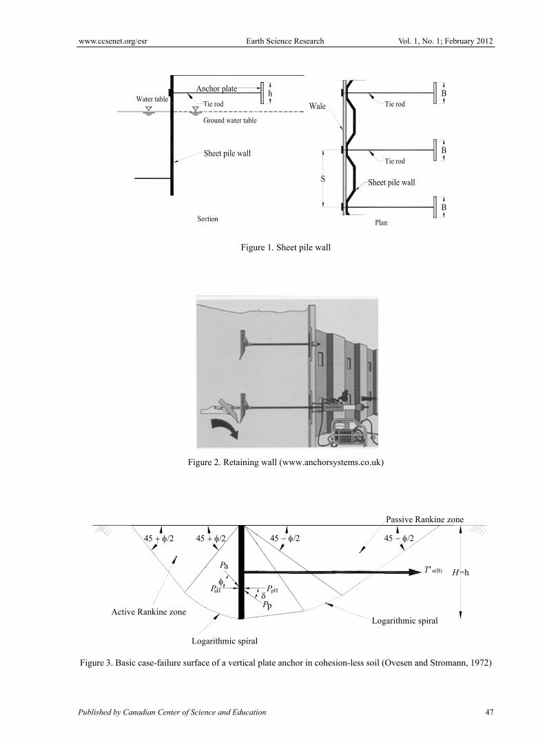
Generally, earth anchors are used to transmit tensile forces from a structure to the soil and to generate passive support to bulkheads, sheet piles and retaining walls (Figures 1 and 2). Their pullout capacity is obtained through the shear strength and dead weight of the surrounding soil. Plate anchors may be made of a steel plate and precast or cast in situ concrete slabs. These anchors can be installed by excavating the ground to the required depth followed by back filling and compacting with a good quality soil.
In the analysis of estimation of ultimate pullout capacity, the vertical plate anchors can be divided in shallow and deep categories. In case of shallow anchors, the embedment ratio is such that, soil above the anchor top can be replaced as a surcharge without shear strength; whereas in case of deep anchors, the embedment ratio is such that, failure surface does not reach the ground surface at limit equilibrium (Das, 1990).
The proposed analysis is confined to shallow laid plate anchors in cohesion-less soil.
2. Previous Experimental Investigations
A number of investigations are reported by several researches to evaluate the ultimate pullout capacity of shallow laid vertical plate anchors.
Ovesen and Stromann (1964, 1972) used the failure mechanism proposed by Hansen (1953) to estimate the earth pressures for the case of a continuous shallow plate anchor flushing with the cohesion-less ground surface, termed as the basic case (H/h = 1), where h is the height of the plate anchor with embedment depth, H (Figure 3). The failure mechanism consists of Rankine (1857) and logarithmic spiral zones (Prandtl-zone) as shown in Figure 3. Based on the above failure mechanism, the ultimate pullout capacity, Tu(B) per unit length of a strip anchor was estimated by Ovesen and Stromann (1964, 1972) by the following expression using horizontal force equilibrium.
aHpHu(B) PPT (1)

www.ccsenet.org/esr Earth Science Research Vol. 1, No. 1; February 2012
ISSN 1927-0542 E-ISSN 1927-0550 28
In the above expression, PpH and PaH are the horizontal components of the passive and active thrusts, which can be estimated using the earth pressure coefficients reported by Caquot and Kerisel (1948).
The expression given in Equation 1 was further modified to estimate the ultimate pullout capacity, Tu per unit width of a strip anchor of width B in cohesion-less soil as,
u(B)0vTRTu (2)
The parameter, R0v in the above equation is given by Dickin and Leung (1985) based on the experimental evidence.
hHC
CR
v
vv /
1
0
00
(3)
Where, C0v = 19 for dense sand and 14 for loose sand.
Neely et al. (1973) performed laboratory tests on plate anchors in dry sand and ultimate resistances of these plates were examined using both limit analysis and the method of stress characteristics. Results of tests on rigid anchor plates in terms of M q , a dimensionless force coefficient, were expressed as 2
u hγ/ BTM q , where is unit weight of soil and B is width of plate anchor.
Das and Seeley (1975) conducted several laboratory model tests to determine the ultimate pullout resistance of shallow vertical anchors and suggested a simple semi-empirical relation for the pullout resistance in a non-dimensional form as the ratio of Tu /Bh2 for square and rectangular anchors. Ultimate pull out capacity for a single anchor of width B was expressed by the following semi-empirical relation.
222.35 hγh/1059.4 BHST nu (4)
Where, S is the shape factor which is a function of H/h and is angle of soil friction in degrees. The value of n varies linearly from 1.8, for B/h = 1 to about 1.68 for B/h = 5.
The capacity of deeper vertical anchors in medium dense sand was investigated by Akinmusuru (1978) for square, circular and rectangular anchors. On the basis of experimental findings, the variation of Tu/h3, a non-dimensional anchor load at ultimate failure with , a non-dimensional embedment coefficient ( = H/h) was presented for an anchor length of 10h in the form of a chart. Akinmusuru (1978) clearly defined the critical embedment depth as the one corresponding to = 6.5.
Dickin and Leung (1983) conducted both centrifuge and conventional chamber tests and reported very thorough investigations on the behaviour of vertical square and rectangular anchors in dense sand. The variations of breakout factor Nγq, and the force coefficient Mq with embedment ratio were separately reported in the form of a chart with Nγq = Tu/γBhH and Mγq = Tu/γBh2. The results obtained by them suggested potentially serious over- predictions of pullout resistance and underestimations of the failure displacements. Such errors arose due to the characteristic stress- dependent behaviour of dense soils.
Hoshiya & Mandal (1984) investigated the capacity of square and rectangular anchors in loose sand. The size of box (40 cm x 30 cm x 40 cm deep) used for testing was very small, which facilitated the testing of 2.54 cm wide and 15.24 cm long plates. This was likely to introduce edge effects into the results. They concluded that, anchor break-out factor, Nγq increased with embedment depth up to a certain embedment ratio before reaching a constant value thereafter.
Naser (2006) carried out theoretical as well as experimental studies on the ultimate pullout capacity of an anchor block of concrete embedded in sand and observed that, anchor thickness contributed to the pullout capacity through base friction forces. This effect was not significant as compared to the passive resistance. Uplifting and tilting of the block at failure was also observed.
3. Previous Theoretical Investigations
Terzaghi (1943) evaluated the resistance of vertical strip anchor plates assuming Rankine (1857) states of passive and active pressures. This approach was adopted in the British civil engineering code of practice. The net resistance Tu, per unit length of a vertical strip anchor was given as )( ap PP , where Pp and Pa are the passive and active thrusts (kN/m) acting on the anchor plate.

www.ccsenet.org/esr Earth Science Research Vol. 1, No. 1; February 2012
Published by Canadian Center of Science and Education 29
Teng (1962) estimated holding capacity of a vertical (strip) plate anchor embedded in granular soil at a relatively shallow depth ( h/H ≤ 1/3 to 1/2), based on Rankine’s (1857) theory of lateral earth pressures. He obtained the expression for ultimate holding capacity as,
apu PPT (5)
Where, Pp and Pa are the passive and active pressure thrusts (kN/m) acting on the anchor plate.
In case of shallow strip anchors, Meyerhof (1968, 1973) used the passive and active coefficients of earth pressure proposed by Caqout and Kerisel (1948) and Sokolovskii (1965) and proposed the following simple relationship for ultimate holding capacity per unit length of a vertical plate anchor in cohesion-less soil.
b2K2/1 HTu (6)
Where, Kb is the pullout coefficient that can be obtained from a graph using soil friction angle.
Using limit analysis and plasticity solutions, Neely et al. (1973) determined the theoretical resistance of continuous (strip) vertical plate anchors in cohesion-less soils for two cases. In the first case, failure surface was assumed to be consisting of a logarithmic spirals and its tangent inclined at (45°-/2) to the horizontal as shown in Figure 4. Soil above top of the anchor was considered to act as a simple surcharge, q {(H-h)} and therefore, the method was termed as the surcharge method.
Shearing resistance of the soil above the anchor top is ignored when H/h is small; therefore the method was subsequently modified by considering shear strength above the top of anchor plate when H/h is considerable and was defined as the Equivalent Free Surface method. The assumed failure surface in soil (Figure 5) is an arc of logarithmic spiral with pole at top of the wall. OB is a straight line which is an equivalent free surface. The shearing resistance of upper layers of soil was included in the calculation by making use of the equivalent free surface concept proposed by Meyerhof (1951) in connection with the bearing capacity of shallow foundations. The normal and shear stresses along OB (p0 and s0, respectively) were calculated using Rankine (1857) active stresses on the vertical surface, OA above the top of the anchor plate as shown in Figure 5.
The above analysis is based on the method of stress characteristics and represents a more refined analytical and numerical attempt to predict the ultimate capacity of the vertical plate anchors but it ignores the active earth pressure distribution behind the anchor plate and the kinematic behaviour of the material.
Rowe and Davis (1982b) reported a two-dimensional finite element analysis incorporating an elasto-plastic soil model. For a continuous vertical plate anchor assumed to be thin and perfectly rigid, the resistance is as given by the following expression.
KRψγγq RRRFM (7)
Where, Fγ is the capacity factor of a smooth anchor resting on soil which deforms plastically at a constant volume ( = 0°), with coefficient of earth pressure at rest, K0 = 1 and Rψ, RR and RK are correction factors for the effects of sand dilatancy, anchor plate roughness and initial stress state respectively. The theoretical data was presented in the form of design charts.
A comparative study of the force coefficient, Mq as obtained from experimental investigations and theoretical methods proposed by Ovesen and Stromann (1972), Neely et al., (1973) was carried out by Dickin and Leung (1983). Significant disparity was observed in the results because they were based on two- dimensional analysis and their application to single anchors required a suitable shape factor. Dickin and Leung (1985) observed that, effect of anchor shape on dimensionless coefficients was due to side shear resistance. They observed failure planes radiating outward involving a soil mass wider than a single anchor itself in the failed body. A dimensionless factor, R0v to account for the influence of anchor geometry on the ultimate resistance was introduced by them as stated previously.
Finite element method is also used by various researchers such as Vemeer and Sutjiadi (1985), Tagaya et al. (1983, 1988), Dickin and King (1997) and Sakai and Tanaka (1998). Unfortunately, only limited results are available from these studies.
Upper and lower bound limit analyses are also reported by Murray and Geddes (1987, 1989), Basudhar and Singh (1994) and Smith (1998) to estimate the capacity of vertical strip anchor plates. Basudhar and Singh (1994)

www.ccsenet.org/esr Earth Science Research Vol. 1, No. 1; February 2012
ISSN 1927-0542 E-ISSN 1927-0550 30
obtained estimates with a generalized lower bound procedure based on finite element method and non-linear programming similar to that of Sloan (1988a). The solutions proposed by Murray and Geddes (1987, 1989) are based on kinematically admissible failure mechanisms (upper bound).
Merifield et al. (2006) presented the results of a rigorous numerical work (linear finite elements coupled with upper and lower bound limit analyses, nonlinear finite elements coupled with lower bound limit analyses and displacement finite elements using Solid Nonlinear Analysis Code (SNAC) - an algorithm developed by Abbo and Sloan, 2000) to estimate the ultimate pullout capacity Tu, for a vertical strip anchor plate in the cohesion-less material. For comparison purposes, numerical and theoretical results of the break-out factor were presented in the form analogous to Terzaghi’s (1943) equation of the bearing capacity of shallow foundations.
Tu = γHhNγ (8)
Where, Nγ is the anchor break-out factor that can be obtained from a graph using soil friction angle
The failure mode (Figure 6) reported by Merifield et al. (2006) for vertical plate anchors indicates that, the soil retained behind the anchor can significantly affect the estimated capacity of shallow anchors. This is particularly the case for loose sands, where the development of a significant active zone behind the anchor is observed. Changing the interface roughness from perfectly rough ( = ) to perfectly smooth ( = 0) led to a reduction in the anchor capacity by as much as 65%.
Naser (2006) analyzed pullout capacity of an anchor block (Figure 7) using limit equilibrium approach.The ultimate pullout capacity (Pu) of a block anchor was obtained from the equilibrium of forces acting on the block by summing them along the horizontal direction and multiplying the lateral earth pressures (passive and active) by the 3-D corrections factor M, to yield the following equation.
bstahphu FFFPPMP (9)
Where, Ft, Fb and Fs are the effective friction forces at the top, bottom and at two sides of the block, N is the normal force, Pph is the effective horizontal passive thrust and Pah is the effective horizontal active thrust (Figure 7). For Coulomb (1776) and log spiral theories, Fb = 0 (as N=0). Pullout capacity of block anchor with Rankine’s theory (1857), corrected for the 3-D effect with the contribution of friction, showed a close agreement with experimental results.
More recently Kumar and Sahoo (2011) used an upper bound theorem of the limit analysis in combination with finite elements for estimation of horizontal pullout capacity of vertical plate anchors embedded in sand. The results were plotted for various combinations of embedment ratio, internal friction angle, of sand, and the anchor-soil interface friction angle, δ. It was observed that, the pullout resistance increased with increasing embedment ratio, friction angle of sand and anchor-soil interface friction angle.
4. Proposed Method
In the proposed analysis of the estimation of pullout capacity of a strip anchor in cohesion-less soil, all the three equation of equilibrium are utilized to obtain the required solution. Both passive and active states of equilibrium on the two sides of anchors are considered in the analysis. The active/passive thrusts along with their points of application are evaluated using Kötter’s (1903) equation. This equation has been used by other researchers such as Dewaikar and Mohapatro (2003) for the computation of bearing capacity factor, Nγ, Deshmukh et al. (2010) for the estimation of breakout capacity of horizontal rectangular/square anchors in cohesion-less soils, Rangari et al. (2010) for the computation of seismic vertical uplift capacity factor for horizontal strip anchors and Kame, Dewaikar and Choudhury (2010a) for the estimation of active thrust and its point of application on a vertical retaining wall with horizontal cohesion-less backfill.
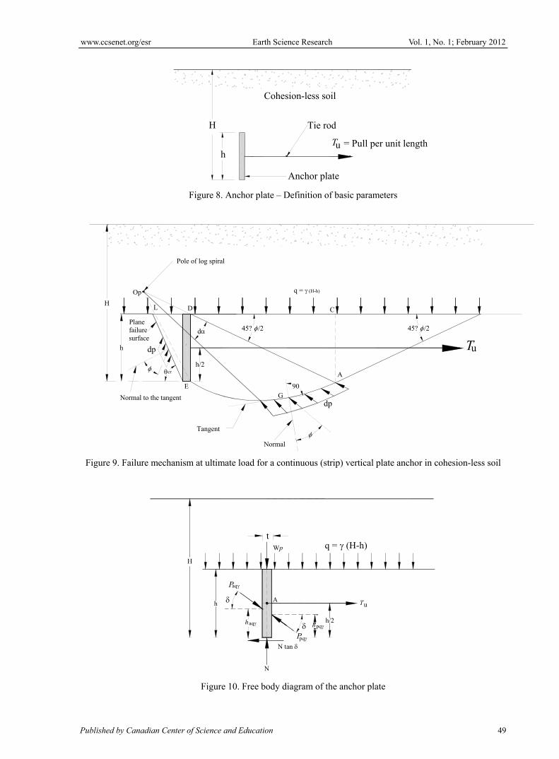
4.1 Geometry of the problem
In Figure 8 is shown a shallow laid continuous (strip) plate anchor buried vertically. The bottom of plate is at a depth, H below the ground surface and h is the height of plate anchor. In case of shallow laid anchors, the ultimate pullout capacity (Tu) is mainly derived from the passive and active resistances of cohesion-less soil in the front and on the back of the anchor plate respectively. The solution to the problem is proposed using Kötter’s (1903) equation coupled with limit equilibrium analysis.
In Figure 9, the failure mechanism adopted in the analysis is shown. In the passive state of equilibrium, the failure surface consists of a log spiral followed by its tangent that meets the ground surface. In the active state of

www.ccsenet.org/esr Earth Science Research Vol. 1, No. 1; February 2012
Published by Canadian Center of Science and Education 31
equilibrium the failure surface is plane as per the Coulomb (1773) mechanism. The anchor plate is shallow laid with embedment ratio, H/h up to 5.
In Figure 10, free body diagram of the strip anchor is shown from which, the following information is generated.
PPq = resultant passive thrust per unit length of the plate anchor
Paq = resultant active thrust per unit length of the plate anchor
= interfacial friction angle
= angle of soil friction
hpq = distance of point of application of passive thrust, Ppq from the anchor base
haq = distance of point of application of active thrust, Paq from the anchor base
Wp = weight of the anchor plate per unit length
t = thickness of the anchor plate
N = upward soil reaction
The parameters Ppq , Paq , hpq and haq are computed using Kötter’s (1903) equation for embedment ratio, H/h up to 5.
4.2 Kötter’s (1903) equation
In a cohesion-less soil medium with passive and active states of equilibrium under plane strain condition, Kötter’s (1903) equation is given as,
sinγd
dtan2
d
d
sp
s
p for the passive state (Figure 11a) (10a)
And
sinγd
dtan2
d
d
sp
s
p for the active state (Figure 11 b) (10b)
In the above equations,
dp = differential reactive pressure on the failure surface
ds = differential length of arc of failure surface
= angle of soil internal friction
dα = differential angle and,
α = inclination of the tangent at the point of interest with the horizontal
For the determination of ultimate pullout capacity using limit equilibrium, the failure mechanism adopted consists of combination of logarithmic spiral and straight lines inclined at 45-/2 to the horizontal in case of passive state of equilibrium and a plane failure surface (Coulomb mechanism, 1773) in case of active state of equilibrium. The soil above the level of the top of the anchor plate is assumed to act as simple surcharge, q kN/m. Contributions to the active/passive thrusts due to surcharge and self-weight are estimated separately using Kötter’s (1903) equation.
4.3 Failure mechanism under the surcharge effect-passive state of equilibrium
In Figure 12 is shown a vertical plate anchor DE, with a horizontal cohesion-less backfill under surcharge loading. Soil unit weight is not considered in the analysis. The failure surface consists of log spiral EA, that originates from the anchor base with tangent AB meeting the ground surface at an angle, (45- /2). At point A, there is a conjugate failure plane AD, passing through the anchor top. Thus, as seen from the figure, ABD is a passive Rankine zone and pole of the log spiral lies on the line AD or its extension.
From Figure 12, the following information is generated.
α = inclination of the tangent to the log spiral at point G with the horizontal
r0 = starting radius of the log spiral at the anchor base (at = 0)
= spiral angle measured from the starting radius
r = radius of log spiral at point G corresponding to the spiral angle

www.ccsenet.org/esr Earth Science Research Vol. 1, No. 1; February 2012
ISSN 1927-0542 E-ISSN 1927-0550 32
m = maximum spiral angle
r1 = radius of the maximum spiral angle at = m
v = angle between vertical face of the plate anchor and the starting radius r0
From Figure 13, which shows the free body diagrams of failure wedge, EACD, the following information is generated.
PpqH, PpqV = horizontal and vertical components of resultant passive thrust, Ppq due to surcharge effect
RpqH, RpqV = horizontal and vertical components of resultant soil reaction, Rpq acting on the curved part of the failure surface
Pq = pasive thrust exerted by the backfill on the Rankine wall, AC
Q = resultant force due to surcharge
In Figure 13, line AC represents the Rankine wall and force, Pq as described above, is the force exerted on this wall by the backfill it retains. With this consideration and also considering that, pole of the log spiral lies above the anchor top on line AD, the dispositions of various forces are shown in the same figure.
4.3.1 Geometry of the failure surface
Referring to Figure 13 and considering triangle, ODE,
mmv sin
h
sin
DE
2)/-135(sin
OE
sin
OD
(11)
Where, angles, m and v are as shown in the same figure.
From the above expression,
m
v
sin
sinhOD
The initial radius, OE = r0 of the log spiral is given as,
m0 sin
2)/-135(sinh OE
r
Also, from the equation of the log spiral,
tan0 .OA mer (12)
And
AD = OA – OD
4.3.2 Computation of vertical and horizontal components of reaction on curved failure surface EA under the effect of surcharge
For the curved failure surface, EGA (Figure 13), Kötter’s (1903) equation (Eq. 10a) takes the following form.
0d
dtan2
d
d
sp
s
p (13)
From quadrilateral, OEJG (Figure 12)
36090180)90( v
With simplification,
0 v
Or,
v
Differentiation with respect to gives,
dd (14)

www.ccsenet.org/esr Earth Science Research Vol. 1, No. 1; February 2012
Published by Canadian Center of Science and Education 33
Combining Eq. 14 with Eq. 13, and multiplying throughout by ds/dα, the following equation is obtained.
dp
tan2p
d (15)
For integration over the curved failure surface, EGA, the above equation is written as,
mA
dp
dpp
p
tan2
Where, pA is the pressure intensity at point A (Figure 13).
Integration yields
tan)(2 mepp A (16)
From Eq. 16, the resultant soil reaction, Rpq on curved surface, EGA is given as,
pdsR pq (17)
Or
dsepR m
Apq tan)(2
From the geometry of log spiral,
dsecd rs (18)
Using above equation, Rpq is obtained as,
dsectan)(2 repR m
Apq (19)
With tan
0err the above equation is transformed to,
dsectan
0tan)(2 erepR m
Apq (20)
From Figure 13, considering DEO
)2/4590(180 vm
Or,
vm 2/45
The angle (FOG) made by the resultant, Rpq (Figure 13) with the horizontal can be obtained from the following expression.
]2/45[)2/45( vFOG
vFOG 90
Or,
LFOG
Where,
VL 90
The vertical component, RpqV (Figure 13) of resultant soil reaction is then obtained as,

www.ccsenet.org/esr Earth Science Research Vol. 1, No. 1; February 2012
ISSN 1927-0542 E-ISSN 1927-0550 34
m
dRR Lpq
0pqV )sin( (21)
Similarly, the horizontal component, RpqH (Figure 4) of soil reaction is obtained as,
m
dRR LpqpqH
0)cos( (22)
4.3.3 Computation of reactive pressure distribution on the plane failure surface AB and reactive pressure at point A under the effect of surcharge
From the geometry of the problem, 0ds
d and Kötter’s (1903) equation (Eq. 10a) takes the following form for a
weightless medium.
0d
ds
p (23)
Integration yields,
constantp (24)
Thus, the reactive pressure, p is uniformly distributed on the failure surface, AB and the resultant reaction, R acts at the mid-point of AB.
To find the reactive pressure, p, equilibrium of failure wedge ABC is considered (Figure 16)
According to Rankine’s theory, the passive thrust, Pq on the wall, AC is given as,
pq KACqP (25)
Where, Kp is the coefficient of passive earth pressure for a horizontal cohesion-less backfill and it is as given by the following expression.
sin1
sin1
pK
Horizontal equilibrium of the failure wedge ABC gives
)2/45cos( RPq (26)
From Eqs. 26 and 27 R is obtained as
pKABqR )2/45tan( (27)
The uniformly distributed soil pressure, p is then obtained as,
ABRp /
Or,
pKqp )2/45tan( (28)
The intensity of reactive pressure, pA at point A (Figures 12 and 14) is as given by the above expression.
From Figure 14, it is further seen that, the three-force equilibrium of the failure wedge, ABC gives the point of application of Pq at mid-point of the wall, AC.
4.4 Failure mechanism under the effect of soil self weight - passive state of equilibrium
Figure 15 shows the failure mechanism similar to that adopted for the analysis of the plate anchor with a horizontal cohesion-less backfill under surcharge effect. Using the above failure mechanism, the authors (2010 b)

www.ccsenet.org/esr Earth Science Research Vol. 1, No. 1; February 2012
Published by Canadian Center of Science and Education 35
have reported a method based on the application of Kötter’s (1903) equation for the estimation of passive thrust on a vertical wall retaining horizontal cohesion-less backfill. The unique failure surface consisting of a log spiral and its tangent is identified on the basis of force equilibrium conditions and point of application of the passive thrust is computed using moment equilibrium. In the proposed analysis, this procedure is adopted to compute the values of passive thrust, Pp under the effect of soil self weight and its point of application. The final expression for the reactive passive pressure distribution at any point on the curved failure surface, EA using Kötter’s (1903) equation is obtained with the following expression.
Lm
Lm2
23tan0
L
L2
tan0
23tan0
cos
sintan3
tan91
secγ
cos
sintan3
tan91
secγ
24Ksinγ
m
m
er
er
er
p (29)
Where, K is the parameter indicating location of the pole of the log spiral along line AO in terms of starting radius of log spiral r0 as measured from point D (Figure 13) and L = (90-V)
The distribution of reactive passive pressure on the failure surface is as shown in Figure 16. The magnitude of passive thrust on the vertical anchor plate and its point of application are thus obtained using Kötter’s (1903) equation.
From Figure 17, the following information is generated.
PpH, PpV = horizontal and vertical components of resultant passive thrust, Pp
R pH, R pV = horizontal and vertical components of resultant soil reaction, Rp acting on the curved part of the failure surface
H1 = passive thrust exerted by the backfill on the Rankine wall AC
WACD = weight of soil in the failure wedge, forming a part of the Rankine zone
WADE = weight of soil in the zone, EAD of the failure wedge, EABCD
Ypp = the distance of point of application of Pp from the anchor top
X = the distance from pole O to the centroid of sector, OEA formed by the log spiral
hp = distance of point of application of passive thrust, Pp from the anchor base
= varying angle of inclination of reactive pressure with the vertical
The resultant soil reaction, Rp (Figure 17) on the failure surface is obtained as,
spRp d.γ (30)
The vertical and horizontal components, RpV and R pH of resultant reaction are obtained as,
spRm
d.cos0
Vpγ
(31)
spRm
Hp d.sin0
γ
(32)
Where, ds is the length of failure surface and is the varying angle of inclination of reactive pressure with vertical (Figure 17). The detailed calculations for estimation of the passive thrust are reported in the paper “Passive thrust on a vertical retaining wall with horizontal cohesion-less backfill” accepted for publication in Soils and Rocks, An International Journal of Geotechnical and Geo-environmental Engineering, Brazil. (Kame, Dewaikar and Choudhury, 2010-b)

www.ccsenet.org/esr Earth Science Research Vol. 1, No. 1; February 2012
ISSN 1927-0542 E-ISSN 1927-0550 36
4.5 Failure mechanism under combined effect of uniform surcharge loading and soil self weight -passive state of equilibrium
The distribution of reactive pressure on the failure surface is computed using Kötter’s (1903) equation under the effect of uniform surcharge and soil self weight.
In Figure 18 is shown the free body diagram of failure wedge EACD for combined effect. The following information is generated from the figure.
PpqH, PpqV = horizontal and vertical components of resultant passive thrust, Ppq under the combined effect.
Rpq = resultant reactive pressure on curved failure surface
4.5.1 Computation of reaction due to combined effect on the curved failure surface EA
The magnitude of vertical component of soil reaction, RpqV for the combined effect is obtained by adding up Eqs. 21 and 31 as,
RpqV = RpqV+ RpV
Or
m
dRR Lpqpq
0Vγ )sin( sp
m
d.cos0
(33)
Similarly the horizontal component soil reaction, R pqH is obtained by adding Eqs. 22 and 32 as,
m
dRR Lpqpq
0Hγ )cos( sp
m
d.sin0
(34)
4.5.2 Magnitude of passive thrust under the combined effect
In Figure 18, the passive Rankine thrust, H1 under the effect of soil self weight and passive thrust, Pq on the wall, AC under the effect of surcharge loading (Eq. 25) act at a distance 1/2AC
and 2/3AC respectively from point, C.
Equilibrium of wedge, EACD is then considered.
Vertical force equilibrium condition gives
QWWsin ADEACDVpqγpqγVpqγ RPP (35)
From which, Ppq is obtained as,
sin
QWW ADEACDVpqγpqγ
RP (36)
In the above equation, Q is the equivalent force due to surcharge (Q = q.DC). It acts at the mid-point of DC.
Horizontal force equilibrium condition gives
1HpqγpqγHpqγ Hcos qPRPP (37)
From which, Ppq is obtained as,
cos
H1Hpqγpqγ
qPR
P (38)
It may be noted that, both Eqs. 36 and 38 give the magnitude of unknown thrust, Ppq. These two equations will yield the same and unique value of Ppq only when the equilibrium conditions correspond to those at failure, which are uniquely defined by a characteristic value of V and this value can be determined by trial and error procedure.
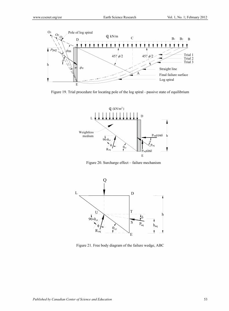
4.5.3 Trial and error procedure for combined analysis - passive state of equilibrium
In this procedure, first a trial value of V (Figure 18) is assumed and corresponding weight of trial failure wedge, EACD and resultant force due to surcharge (Figure 18) are computed. Using Eqs. 33 and 34, magnitudes of

www.ccsenet.org/esr Earth Science Research Vol. 1, No. 1; February 2012
Published by Canadian Center of Science and Education 37
vertical and horizontal components of soil reaction (RpqV and R pqH) are computed and from Eqs. 36 and 38, values of Ppq are determined. If the trial value of V is equal to its characteristic value corresponding to the failure condition, the two computed values of Ppq will be the same; otherwise, they will be different. For various trial values of V, computations are carried out till the convergence is reached to a specified (third) decimal accuracy. Thus, in this method of analysis, the unique failure surface (Figure 19) is identified by locating the pole of log spiral in such a manner that, force equilibrium condition of failure wedge, EACD is satisfied.
4.5.4 Point of application of passive thrust under the combined effect
Moment equilibrium condition is now used to compute the point of application of passive thrust by considering moments of forces and reactions about the pole of the log spiral.
Referring to Figure 18, for pole above anchor top, the following moment equilibrium equation is obtained by considering moment of the various forces about the pole of the log spiral.
OFP)5.0(
)5.0(FDAC3
2
XWDC)3
2OF(W
)FD(Y
Vpqγ
1
ADEACD
pqγHpqγ
ACFDP
DCOFQHP
q
(39)
In the above equation, terms on the right hand side represent moment of weight of soil in the failure wedge, EACD, moment of the force Q, moment of the forces H1 and Pq and moment due to vertical component of the resultant passive thrust, PpqV about the pole, O. The term on the left hand side of the above expression is the moment due to horizontal component of the resultant passive thrust, PpqH about the pole, O. From the above equation, Ypq (which is the distance of point of application of Ppq from the anchor top), is obtained as,
FD-OFP)5.0(
)5.0(FDAC3
2
XWDC)3
2OF(W
1Y
HpqγVpqγ
1
ADEACD
Hpqγpqγ
PACFDP
DCOFQHP
q
(40)
The height, hpq of the passive thrust, Pp from the anchor base is then obtained as,
pqγγ Yh pqh
The basic purpose of this analysis was to compute passive pressure thrust, Ppq along with its location and study their variation with respect to the parameters involved in the analysis. The height, hpq of point of application of passive thrust from the anchor base is expressed in terms of its ratio with respect to the height, h of the plate anchor in a non-dimensional form (hrq = h pq /h).
4.6 Failure mechanism under the surcharge effect - active state of equilibrium
In Figure 20 is shown a vertical anchor plate DE, with horizontal cohesion-less backfill under surcharge loading. Soil unit weight is not considered in the analysis. The failure surface, EL is assumed to be plane (Das, 1990). The reaction, Raq on the failure surface is inclined with normal at an angle, (Coulomb, 1776).
4.6.1 Computation of active thrust
The inclination, cr of the failure plane EL, with the horizontal gives maximum value of Paq as per the procedure available in any text book.
4.6.2 Point of application of Paq
This computation is facilitated using Kötter’s (1903) equation (Figure 11 b) for a cohesion-less soil medium under active condition as given below.
For the present analysis = 0 and with this modification Eq. 10b is written as,

www.ccsenet.org/esr Earth Science Research Vol. 1, No. 1; February 2012
ISSN 1927-0542 E-ISSN 1927-0550 38
tan2pd
dp (41)
Or
dpdp tan2 (42)
For a plane failure surface, d is zero and the above equation finally becomes,
dp = 0 (43)
The corresponding solution is obtained as,
p = constant (44)
The above solution indicates that, soil reactive pressure; p is uniformly distributed along the failure plane, EL. Therefore, the resultant soil reaction, Raq acts at the mid-point of the failure plane. Free body diagram of the failure wedge is shown in Figure 21.
In Figure 21 the distance, TU is 0.5DL or 0.5h/tancr. The force, Q of surcharge acts at the mid-point of DL and therefore, meets the force, Raq at U. The three force equilibrium requires that, line of the active thrust, Paq should also pass through point U and this facilitates computation of its point of application.
The distance haq of point of application of Paq as measured from the wall base is then given as,
crtan
tan15.0
hhaq (45)
4.6.3 Active thrust under the effect of soil self weight
For this analysis, the method proposed by Dewaikar et al. (2003) is used. The angle, θcr of the failure plane EL is obtained using trial and error procedure, coupled with Kötter’s (1903) equation.
For a plane failure surface, d is zero and Kötter’s (1903) equation as given above takes the following form.
dsdp ).sin( (46)
Integration yields,
1).sin( Csp (47)
At point L, both p and s are zero and with this condition the constant C1 works out to be zero. Therefore, the reactive pressure, p on the failure surface is finally expressed as,
sp ).sin( (48)
To compute reaction, Ra, the above expression is integrated within the limits s = 0 (at point L) to s = length EL (at point E).
dssRAC
a 0
).sin( (49)
2)sin(5.0 ACRa (50)
From Figure 23, length EL can be written as,
EL = h/sin (51)
Substitution of the above value of EL in the expression for Ra gives
22
a /sinh )-(sin γ0.5 = R (52)
Now referring to Figure 23, the vertical force equilibrium gives
www.ccsenet.org/esr Earth Science Research Vol. 1, No. 1; February 2012
Published by Canadian Center of Science and Education 39
0)90sin(sin aa RPW (53)
In the above equation, W is the weight of the wedge, DLE.
Or
0)90sin(sin
h )-(sin γ0.5sin
2
2
aPW (54)
From which, Pa is obtained as,
sin
)90sin(sin
h )-(sin γ0.52
2
W
Pa (55)
Again refering to Figure 23, horizontal force equilibrium gives,
)90cos(
sin
)sin(5.0cos
2
2
hPa (56)
Eqs. (55) and (56) will yield the same value of Pa for the critical value of θ, denoted as θcr.
Therefore in the analysis, various trial values of θ are chosen and when the two values of Pa (Eqs. 55 and 56) match each other (up-to three decimal places), trials are terminated.
The reaction Ra corresponding to θcr is then computed as,
2
2
)(sin
)sin(5.0
cr
cra
hR
(57)
4.6.4 Point of application of Pa
For this purpose, first point of application of Ra is computed. Referring to Figure 23, in which the angle, is now θcr, moments of elemental reactive forces about the anchor base are considered.
The elemental reaction, dRa at any point on the failure plane EL is computed as
dsscr )sin(dRa (58)
The moment, dM1 of normal component of elemental reaction about the wall base is given as,
dssh
scr
cr
sin
sin)sin(dM1 (59)
Integration yields the total moment M1.
crH
crcr dsss
hM
sin/
01 sin
sin)sin( (60)
6/sin
sin)sin(3
crcr
h
(61)
The moment, M2 of normal component of total reaction, Ra about the anchor base is expressed as,
cr
cra
xhxRM
2
2
2sin
sin)sin(5.0sin
(62)

www.ccsenet.org/esr Earth Science Research Vol. 1, No. 1; February 2012
ISSN 1927-0542 E-ISSN 1927-0550 40
Where, x is the distance of Ra from the anchor base, along the failure surface, EL.
Equating the expressions as given by Eqs. 61 and 62, x is finally computed as,
3
EL
3
sin crh
x
(63)
Thus, the reactive force, Ra acts at a distance of 1/3 EL as measured from the anchor base. From Figure 23, it is further seen that, distance ET is equal to h/3, since forces Pa, W and Ra meet at point U which is located such that EU = EL /3.
The point of application of Pa is finally computed by considering the following geometry from Figure 23.
tan.UTETha and UT = 1/3DL = h/(3tan) (64)
Where ha is the height of Pa above the anchor base.
4.7 Active thrust under combined effect
The values of Paq and Raq (Figure 24) can be obtained by varying the inclination of failure plane EL so as to identify critical value cr giving maximum value of Paq and corresponding value of R aq.
From the results obtained for Paq, Pa it is seen that, the angle cr that maximizes the active thrust, remains the same in all the cases (surcharge effect, soil self weight effect and combined effect) and therefore the summation of active thrust values (Paq, Pa) exactly matches with the values Paq that is computed for the combined effect.
4.7.1 Point of application of Paq
The principle of superposition leads to the computation of point of application of active thrust, Paq using moment equilibrium about the anchor base. The following expression is obtained.
aq
aaaqaqaq P
hPhPh
.. (65)
Where,haq is the distance of point of application of Paq as measured from anchor base.
4.8 Analysis of the plate anchor
Referring to Figure 10, all the three equilibrium conditions are examined.
4.8.1 Vertical equilibrium
The forces involved are Ppqsin and N in the vertically upward direction and Paqsin and Wp in the vertically downward direction. Since Ppq sin > Paq sin and weight, Wp of the plate is small enough, there is no equilibrium of the forces in the vertical direction. The reaction, N is zero and the plate accelerates in the vertically upward direction. This agrees well with the experimental observation (Naser, 2006).
4.8.2 Moment equilibrium
The forces N and Ntan now can be considered to be zero and the moment equilibrium is considered about the point, A as shown in Figure 10. The only forces that contribute to the moment equilibrium are Paq and Ppq and since Ppq > Paq, clearly moment equilibrium is also not satisfied. The plate rotates at limit equilibrium and this agrees well with the experimental observation (Naser, 2006).
4.8.3 Horizontal equilibrium
Summing up the forces in horizontal direction the following expression is obtained.
coscos aqpqu PPT (66)
As stated earlier, Paq and Ppq are evaluated using Kötter’s (1903) equation and thus Tu is determined from the horizontal equilibrium condition.
The values of Tu are computed using the available experimental data and comparisons with the available theoretical solutions are made.
5. Results and Discussions
For the purpose of comparison, detailed information on the available theoretical solutions and the proposed method is reported in Table 1.

www.ccsenet.org/esr Earth Science Research Vol. 1, No. 1; February 2012
Published by Canadian Center of Science and Education 41
The non-dimensional pullout force coefficient, Mq is defined using following expression.
2Bh
TqM u
(67)
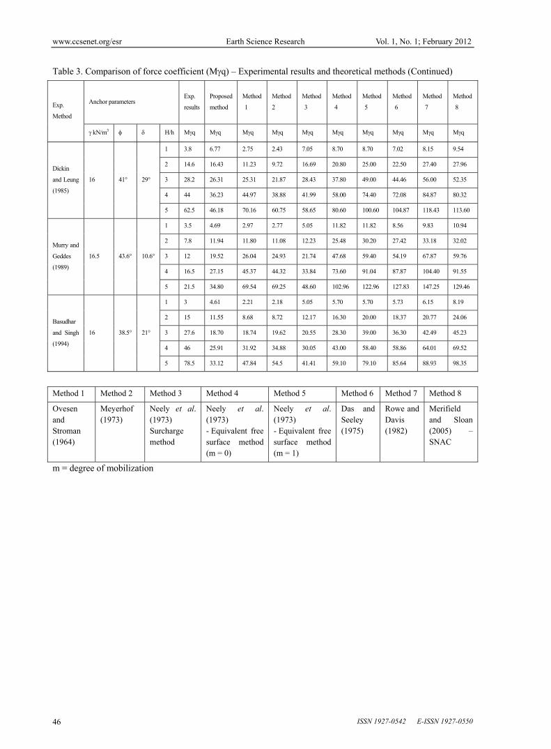
In the present analysis, for a vertical strip plate anchor (H/h = 1 to 5) a total of eight experimental studies (Neely et al., 1973; Das and Seeley, 1975; Akinmusuru, 1978; Ovesen and Stroman, 1964; Dickin and Leung, 1985; Hoshiya and Mandal, 1984; Murray and Geddes, 1987; Rowe and Davis, 1982 and Basudhar and Singh, 1994) and a total of eight theoretical methods (Ovesen and Stroman, 1964; Meyerhof, 1973; Neely et al., 1973, Surcharge method; Neely et al., 1973, Equivalent Free Surface Method (m = 0); Neely et al., 1973, Equivalent Free Surface Method (m = 1); Das and Seeley, 1975; Rowe and Davis, 1982 and Merifield and Sloan, 2005, SNAC) are referred for comparison with the proposed solution and the results are reported in Table 3. In addition to this, computations are performed for (i) different values of H/h ranging from 0 to 5, (ii) different values of varying from 20 to 45 with an interval of 5, and (iii) three values of δ, namely 0, 0.5 and . The numerical results obtained from the analysis are summarized below
In Table 2, the results reported by Kumar and Sahoo (2011), Soubra (2000), and Chen (1975) using the upper bound limit analysis are compared with those obtained by the proposed method. The results obtained by Kumar (2002) using upper bound analysis based on bilinear and composite logarithmic spiral failure are also reported in the table.
The comparison shows that, proposed values are higher than all the earlier reported values. However with increasing and , the difference becomes less.
The values of force coefficient (Mq) as computed by the proposed method are reported in Table 3 along with corresponding experimental results and the prediction based on the available theoretical methods. A wide variation is seen in the results. However it is seen that, up-to the embedment ratio of H/h = 3, the proposed method shows a reasonable agreement with the available experimental data.
In Figure 25, the results obtained by the proposed method are compared with the experimental results reported by Ovesen and Stroman (1964) vis-a-vis other theoretical predictions. It is seen that, there is a large difference between the theoretical predictions and the experimental results in respect to value of Mq. As compared to the proposed method, the experimental results of Ovesen and Stroman (1964) are on the lower side.
As seen from Table 3, results of the proposed method compare well with the theoretical results reported by Neely et al. (1973, surcharge method, equivalent free surface method with m = 0) up to the embedment ratio of 3. From Table 2 it is further seen that, there is a good agreement between results of the proposed method and the Meyerhof’s (1973) method up-to embedment ratio of 5 with the maximum difference of 14%.
In Figure 26, the experimental results of Neely et al. (1973) are compared with the results predicted by various available theoretical methods.
It is seen that, the proposed method and methods proposed by Ovesen and Stroman (1964), Meyerhof (1973), Neely et al. (1973) show a good agreement with the experimental results up to the embedment ratio of 3.
The data reported in Table 3 further shows that, results of the proposed method and the other theoretical methods when compared with the experimental data of Akinmusuru (1978) and Hoshiya and Mandal (1984) show large differences. However, the values of Mq as obtained by the proposed method and those of Ovesen and Stroman (1964) and Meyerhof (1973), show a reasonably good agreement up-to the embedment ratio of 3.
In Figure 27, a comparison is shown between the experimental results reported by Das and Seeley (1975) and the results predicted by various theoretical methods. It is seen that, the methods proposed by Rowe and Davis (1982) and Merifield and Sloan (2005) show a better agreement with experimental results for all embedment depths. The methods proposed by Neely et al. (1973, m = 0 and 1), Das and Seeley (1975) and the proposed method show a fair agreement with experimental results up-to embedment ratio of 3.0.
The experimental data reported by Dickin and Leung (1985) is compared with the available theoretical solutions as shown Figure 28. The proposed method and the method by Neely et al. (1973, surcharge method) perform better than the other methods whereas, the method of Ovesen and Stroman (1964) and Neely et al. (1973, equivalent free surface method, m = 0) show a reasonably good agreement with the experimental results. The equivalent free surface method Neely et al. (1973, m = 1), method of Das and Seeley (1975), Rowe and Davis (1982) and Merifield and Sloan (2005) overestimate the results.
From the above discussion it is clearly seen that, there is no unique theoretical solution for the analysis of a vertical plate anchor in cohesion-less soil. The proposed method is intended for shallow laid anchors only and with this limitation, it shows a reasonably good agreement with some of the experimental/theoretical results up-to the embedment ratio of 3.0.

www.ccsenet.org/esr Earth Science Research Vol. 1, No. 1; February 2012
ISSN 1927-0542 E-ISSN 1927-0550 42
6. Conclusions
A numerical method based on the application of Kötter’s (1903) equation is proposed for the estimation of pullout capacity of shallow laid vertical plate anchors in cohesion-less soil. The unique failure surfaces under active and passive state of limit equilibrium are identified on the basis of force equilibrium conditions. Kötter’s (1903) equation facilitates the computation of point of application of active and passive thrusts.
Comparison of the results of the proposed method with the available experimental results vis-a-vis other theoretical methods shows that, up-to embedment ratio of 3.0, the proposed method is capable of making reasonably good predictions.
References
Abbo, A. J., & Sloan, S. W. (2000). SNAC users manual Version 2.0.
Akinmusuru, J. O. (1978). Horizontally loaded vertical anchor plate in sand, J. Geotech. Engrg. Div., ASCE, 104(2), 283-286.
Anchor Systems Europe. [Online] Available at: www.anchorsystems.co.uk
Basudhar, P. K. & Singh, D. N. (1994). A generalized procedure for predicting optimal lower bound break-out factors of strip anchors. Geotechnique, 44(2), 307-318. http://dx.doi.org/10.1680/geot.1994.44.2.307
Caquot, A. I., & Kerisel, J. (1948). Tables for the calculation of passive pressure, active pressure, and bearing capacity of foundations. Libraire du Bureau des Longitudes, de L’ecole Polytechnique, Paris Gauthier- villars, Imprimeur-Editeur, 120.
Chen, W. F. (1975). Limit analysis and soil plasticity. Developments in Geotechnical Engineering, Elsevier, Amsterdam.
Coulomb, C. A. (1776). Essais sur une application des regles des maximis et minimis a quelques problems de statique relatits a l'architecture. Mem. Acad. Roy. Pres. Divers, Sav., Paris 5, 7.
Das, B. M. & Seeley, G. R. (1975). Load-displacement relationship for vertical anchor plates. J. Geotech. Eng. Div., ASCE, 101(7), 711-715.
Das, B. M. (1990). Earth Anchors. J. Ross Publishing, Inc. Australia. (Chapter 3).
Deshmukh, V. B., Dewaikar D. M. & Deepankar Choudhury. (2010). Analysis of rectangular and square anchors in cohesion-less soil. Int. J. of Geotech. Eng., 4, 79-87. http://dx.doi.org/10.3328/IJGE.2010.04.01.79-87
Dewaikar, D. M. & Mohapatro B. G. (2003). Computation of bearing capacity factor N-Terzaghi’s mechanism. Int. J. Geomech., ASCE 3(1),123-128. http://dx.doi.org/10.1061/(ASCE)1532-3641(2003)3:1(123)
Dickin, E. A., & King, G. W. (1997). Numerical modeling of the load–displacement behavior of anchor walls. Comput Struct, 63(4), 849-858. http://dx.doi.org/10.1016/S0045-7949(96)00066-1
Dickin, E. A. & Leung, C. F. (1985). Evaluation of design methods for vertical anchor plates, J. Geotech. Eng., ASCE, 111(4), 500-520.
Dickin, E. A., & Leung, C. F. (1983). Centrifuge model tests on vertical anchor plates. J. of Geotech. Eng., 109, 12, 1503-1525. http://dx.doi.org/10.1061/(ASCE)0733-9410(1983)109:12(1503)
Hoshiya, M., & Mandal, J. N. (1984). Some studies of anchor plates in sand. Soils and Found., Japan , 24(1), 9-16.
Kame, G. S., Dewaikar, D. M., & Deepankar Choudhury. ( 2010-a). Active thrust on a vertical retaining wall with cohesion-less backfill. EJGE, 15(Q), 1848-1863. www.ejge.com/2010/Ppr10.134/Ppr10.134.pdf
Kame, G. S., Dewaikar, D. M., & Deepankar Choudhury. ( 2010-b). Passive thrust on a vertical retaining wall with horizontal cohesion-less backfill. Soils and Rocks, Int. J. of Geotech. and Geo-env. Eng., Brazil.(in press).
Kötter, F. (1903). Die Bestimmung des Drucks an gekrümmten Gleitflächen, eine Aufgabe aus der Lehre vom Erddruck Sitzungsberichte der Akademie der Wissenschaften. Berlin, 229-233.
Kumar, J. (2002). Seismic horizontal pullout capacity of vertical anchors in sands, Can. Geotech. J., 39(4), 982-991. http://www.nrcresearchpress.com/doi/abs/10.1139/t02-021?journalCode=cgj
Kumar, J., & Sahoo, J. P. (2011). An upper bound solution for pullout capacity of vertical anchors in sand using finite elements and limit analysis. International Journal of Geomechanics. ASCE (in press) http://dx.doi.org/10.1061/(ASCE)GM.1943-5622.0000160
Merifield, R. S., Sloan, S. W., & Yu, H. S. (2006). The Ultimate Pullout Capacity of Anchors in Frictional Soils. Can. Geotech. J., 43(8), 852-868. http://www.newcastle.edu.au/research-centre/cgmm/publications/richard-merifield.html
www.ccsenet.org/esr Earth Science Research Vol. 1, No. 1; February 2012
Published by Canadian Center of Science and Education 43
Meyerhof, G. G. (1973). Uplift resistance of inclined anchors and piles. Proceedings, 8th International onference on Soil Mechanics and Foundation Engineering, Moscow, 2, 167-172.
Meyerhof, G. G., & Adams, J. I. (1968). The Ultimate Uplift Capacity of Foundations. Can. Geotech. J., 5(4), 225-244. http://dx.doi.org/10.1139/t68-024
Murray, E. J., & Geddes, J. D. (1987). Uplift of anchor plates in sand. J. Geotech. Eng., ASCE, 113(3), 202-215. http://www.murrayrix.co.uk/papers_and_publications.asp
Murray, E. J., & Geddes, J. D. (1989). Resistance of passive inclined anchors in cohesion-less medium. Geotechnique, 39(3), 417-431. http://www.murrayrix.co.uk/papers_and_publications.asp
Naser, A. S. (2006). Pullout capacity of block anchor in unsaturated sand. Unsaturated Soils 2006 (GSP 147) Proceedings of the Fourth International Conference on Unsaturated Soils., ASCE, 403-414. doi:10.1061/40802(189)29
Neely, W. J., Stuart, J. G., & Graham, J. (1973). Failure loads of vertical anchor plates in sand. J. Soil Mech. and Found. Div., ASCE, 99(9), 669-685.
Niroumand, H., & Kassim, K. A. (2010). Analytical and numerical studies of vertical anchor plates in cohesion-less soils. EJGE, 15(L), 1140-1150. www.ejge.com/2010/Ppr10.089/Ppr10.089.pdf
Ovesen, N. K. ( 1964). Anchor slabs calculation methods and model tests. Danish Geotech. Inst., Copenhagen, Denkark. Bull. No. 16, 5. http://www.geo.dk/bulletiner.aspx
Ovesen, N. K., & Stromann, H. (1972). Design method for vertical anchor slabs in sand. Proceedings of Specialty Conf. on Performance of Earth and Earth-Supported Structures, 1-2, 1418-1500.
Rangari, S., Choudhury, D., & Dewaikar, D. M. (2010). Computation of seismic vertical uplift capacity factor fd for horizontal strip anchors using Kötter’s equation. Proceeding of Int. conf. on disaster prevention technology and management, Chongqing, China, 3(4), 610, October.
Rankine, W. (1857). On the stability of loose earth. Philosophical Transactions of the Royal Society of London, 147. http://dx.doi.org/10.1098/rstl.1857.0003
Rowe, R. K., & Davis, H. (1982b). The Behavior of Anchor Plates in Sand. Geotechnique, 32(1), 25-41. http://dx.doi.org/10.1680/geot.1982.32.1.25
Sakai, T., & Tanaka, T. (1998). Scale effect of a shallow circular anchor in dense sand. Soils and Found., Japan, 38(2), 93-99.
Sloan, S. W. (1988a). Lower bound limit analysis using finite elements and linear programming. International Journal for Numerical and Analytical Methods in Geomechanics, 12, 61-67. http://dx.doi.org/10.1002/nag.1610120105
Smith, C. S. (1998). Limit loads for an anchor/trapdoor embedded in an associated coulomb soil. Int. J. Num. and Anal. Meth. Geomech., 22, 855-865. http://dx.doi.org/10.1002/(SICI)1096-9853(199811)22:11<855::AID-NAG945>3.0.CO;2-4
Sokolovski, V. V. (1965). Statics of granular media. Oxford: Pergamon.
Soubra, A. H., & Macuh, B. (2002). Active and passive earth pressure coefficients by a kinematical approach. Proc. of the Institution of Civil Engineers Geotechnical Engineering, 155(2), 119-131.
Tagaya, K., Scott, R. F., & Aboshi, H. (1988). Pullout resistance of buried anchor in sand. Soils and Found., Japan, 28(3), 114-130.
Tagaya, K., Tanaka, A., & Aboshi, H. (1983). Application of finite element method to pullout resistance of buried anchor. Soils and Found., Japan, 23(3), 91-104.
Teng, W. C. (1962). Foundation design. Prentice-Hall, Englewood cliffs, New Jersey, USA.
Terzaghi, K. & Peck, R. B. (1967), Soil mechanics in engineering practice, John Wiley and Sons, Inc., New York, N.Y.
Vermeer, P. A., & Sutjiadi, W. (1985). The uplift resistance of shallow embedded anchors. Proceedings, 11th International Conference on Soil Mechanics and Foundation Engineering, San Francisco, 4, 1635-1638.

www.ccsenet.org/esr Earth Science Research Vol. 1, No. 1; February 2012
ISSN 1927-0542 E-ISSN 1927-0550 44
Table 1. Comparison of the proposed method with the available theoretical solutions
Name Authors Method adopted Failure mechanism/ model adopted
Comments
Method 1 Ovesen and Stromann (1964)
Limit equilibrium (1948)
Failure mechanism proposed by Hansen (1953)
Use of earth pressure coefficients reported by Caquot and Kerisel (1948)
Method 2 Meyerhof (1973)
Semi-empirical (1965) Logarithmic spiral
Use of earth pressure coefficients reported by Caquot and Kerisel (1948) and Sokolovskii (1965)
Method 3 Neely et al. (1973)
Surcharge method (limit analysis and plasticity solutions)
Logarithmic spiral and its tangent
Pole of the logarithmic spiral is assumed to be located at anchor top and resistance due to active earth pressures is neglected
Methods 4 and 5
Neely et al. (1973)
Equivalent free surface method (m = 0, 1)
m=degree of mobilization of shear strength
Logarithmic spiral
Pole of the logarithmic spiral is assumed to be located at anchor top and resistance due to active earth pressures is neglected
Method 6 Das and Seeley (1975)
Semi-empirical Based on laboratory model tests
Use of chart/graph
Method 7 Rowe and Davis (1982)
Two-dimensional finite element analysis
Elasto-plastic soil model
Use of design charts
Method 8 Merifield and Sloan (2005)
Finite element analysisSolid Nonlinear Analysis Code (SNAC)
Use of chart/graph
Method 9 Kumar and Sahoo (2011)
Upper bound theorem of the limit analysis in combination with finite elements
Elasto-plastic soil model
Use of chart/graph
Proposed method
Kame et al. (2011)
Kötter’s (1903) equation coupled with limit equilibrium analysis
Log spiral and its tangent
All equilibrium equations are used.
Table 2. Comparison of force coefficient (Mq) for H/h = 1
/ Proposed method
Kumar and Sahoo (2011)
Method 9
Kumar (2002) Chen (1975) Soubra (2000) Bilinear Log-spiral Bilinear Log-spiral
30
0 1.71 1.37 1.50 1.50 1.50 1.50 1.50
0.5 2.42 2.15 2.28 2.28 2.28 2.28 2.27
1 3.16 2.80 3.14 3.07 3.14 3.07 2.97
40
0 2.73 2.24 2.30 2.30 2.30 2.30 2.30
0.5 4.96 4.64 4.76 4.74 4.75 4.75 4.70
1 8.14 7.42 8.71 8.01 8.70 8.01 7.51

www.ccsenet.org/esr Earth Science Research Vol. 1, No. 1; February 2012
Published by Canadian Center of Science and Education 45
Table 3. Comparison of force coefficient (Mq) – Experimental results and theoretical methods
Exp.
Method
Anchor parameters Exp.
results
Proposed
method
Method
1
Method
2
Method
3
Method
4
Method
5
Method
6
Method
7
Method
8
kN/m3 H/h Mq Mq Mq Mq Mq Mq Mq Mq Mq Mq
Ovesen and
Stroman
(1964)
16.77 42° 38.66°
1 2.83 9.43 2.96 2.56 9.26 9.90 9.90 7.59 8.77 10.08
2 7.6 21.73 12.16 10.24 21.72 22.60 27.00 24.31 29.56 29.52
3 15 34.22 27.65 23.04 36.85 41.60 53.00 48.04 60.43 55.20
4 23.6 46.75 49.50 40.96 54.20 64.00 80.80 77.90 92.15 84.64
5 32.87 59.29 77.81 64 75.13 89.20 109.20 113.33 129.17 119.70
Neely et al.
(1973) 15.9 38.5° 21°
1 3.5 4.61 2.44 2.18 5.05 5.70 5.70 5.73 6.15 8.19
2 13.5 11.55 10.03 8.72 12.17 16.30 20.00 18.37 20.77 24.06
3 27 18.70 22.63 19.62 20.55 28.30 39.00 36.30 42.49 45.23
4 45 25.90 40.22 34.88 30.05 43.00 58.40 58.86 64.01 69.52
5 75 33.11 62.77 54.5 41.41 59.10 79.10 85.64 88.93 98.35
Das and
Seeley
(1975)
15.92 34° 34°
1 5.1 4.47 1.96 1.82 4.48 4.62 4.70 3.84 3.93 5.76
2 16 10.91 8.19 7.28 11.16 11.80 14.00 12.31 12.84 17.04
3 31 16.37 18.55 16.38 18.70 20.80 26.00 24.33 25.99 32.40
4 50 21.03 33.00 29.12 28.00 31.60 39.00 39.45 40.21 50.08
5 74 25.17 51.53 45.5 37.60 45.60 53.60 57.39 56.94 70.90
Akinmusuru
(1978) 15.55 35° 29°
1 8 4.37 1.95 1.9 4.42 5.10 5.10 4.22 4.23 6.30
2 21 10.73 7.94 7.6 10.97 13.00 15.00 13.52 13.83 18.60
3 38 17.23 17.59 17.1 18.29 23.00 28.00 26.71 28.01 35.25
4 60 23.77 30.71 30.4 27.26 35.00 42.00 43.31 43.12 54.40
5 88 30.31 47.10 47.5 36.57 50.00 58.00 63.01 60.84 77.00
Hoshiya and
Mandal
(1984)
14.12 29.5° 29.5°
1 3.4 3.03 1.54 1.465 5.50 2.90 2.90 2.43 2.74 3.50
2 14.5 7.49 6.58 5.86 13.53 8.05 9.50 7.79 8.93 10.52
3 34 11.24 14.87 13.185 22.18 14.20 17.00 15.40 18.06 20.46
4 62 14.43 26.34 23.44 33.13 20.70 25.50 24.97 28.67 31.96
5 99 17.27 40.93 36.625 44.37 28.00 33.80 36.33 41.31 45.30
Method 1 Method 2 Method 3 Method 4 Method 5 Method 6 Method 7 Method 8
Ovesen and Stroman (1964)
Meyerhof (1973)
Neely et al. (1973) Surcharge method
Neely et al. (1973) - Equivalent free surface method (m = 0)
Neely et al. (1973) - Equivalent free surface method (m = 1)
Das and Seeley (1975)
Rowe and Davis (1982)
Merifield and Sloan (2005) – SNAC
m = degree of mobilization
www.ccsenet.org/esr Earth Science Research Vol. 1, No. 1; February 2012
ISSN 1927-0542 E-ISSN 1927-0550 46
Table 3. Comparison of force coefficient (Mq) – Experimental results and theoretical methods (Continued)
Exp.
Method
Anchor parameters Exp.
results
Proposed
method
Method
1
Method
2
Method
3
Method
4
Method
5
Method
6
Method
7
Method
8
kN/m3 H/h Mq Mq Mq Mq Mq Mq Mq Mq Mq Mq
Dickin
and Leung
(1985)
16 41° 29°
1 3.8 6.77 2.75 2.43 7.05 8.70 8.70 7.02 8.15 9.54
2 14.6 16.43 11.23 9.72 16.69 20.80 25.00 22.50 27.40 27.96
3 28.2 26.31 25.31 21.87 28.43 37.80 49.00 44.46 56.00 52.35
4 44 36.23 44.97 38.88 41.99 58.00 74.40 72.08 84.87 80.32
5 62.5 46.18 70.16 60.75 58.65 80.60 100.60 104.87 118.43 113.60
Murry and
Geddes
(1989)
16.5 43.6° 10.6°
1 3.5 4.69 2.97 2.77 5.05 11.82 11.82 8.56 9.83 10.94
2 7.8 11.94 11.80 11.08 12.23 25.48 30.20 27.42 33.18 32.02
3 12 19.52 26.04 24.93 21.74 47.68 59.40 54.19 67.87 59.76
4 16.5 27.15 45.37 44.32 33.84 73.60 91.04 87.87 104.40 91.55
5 21.5 34.80 69.54 69.25 48.60 102.96 122.96 127.83 147.25 129.46
Basudhar
and Singh
(1994)
16 38.5° 21°
1 3 4.61 2.21 2.18 5.05 5.70 5.70 5.73 6.15 8.19
2 15 11.55 8.68 8.72 12.17 16.30 20.00 18.37 20.77 24.06
3 27.6 18.70 18.74 19.62 20.55 28.30 39.00 36.30 42.49 45.23
4 46 25.91 31.92 34.88 30.05 43.00 58.40 58.86 64.01 69.52
5 78.5 33.12 47.84 54.5 41.41 59.10 79.10 85.64 88.93 98.35
Method 1 Method 2 Method 3 Method 4 Method 5 Method 6 Method 7 Method 8
Ovesen and Stroman (1964)
Meyerhof (1973)
Neely et al. (1973) Surcharge method
Neely et al. (1973) - Equivalent free surface method (m = 0)
Neely et al. (1973) - Equivalent free surface method (m = 1)
Das and Seeley (1975)
Rowe and Davis (1982)
Merifield and Sloan (2005) – SNAC
m = degree of mobilization
www.cc
Publish
Figure
csenet.org/esr
hed by Canadian
Active Rank
e 3. Basic case
n Center of Scien
Figur
kine zone
Log
-failure surfac
Ear
nce and Educati
Figu
re 2. Retaining
aP
PaH
garithmic spiral
e of a vertical
rth Science Rese
ion
ure 1. Sheet pil
g wall (www.a
Pp
PpH
l
plate anchor in
earch
le wall
anchorsystems.
n cohesion-les
Vol.
.co.uk)
Passive
Logarithmi
ss soil (Ovesen
. 1, No. 1; Febru
H=
T u(B)
e Rankine zone
ic spiral
n and Stromann
uary 2012
47
=h
e
n, 1972)

www.ccsenet.or
48
Figure 6. Fai
rg/esr
Fi
ilure modes an
Fi
H
Figure 4.
OH
h
A
igure 5. Equiva
nd zones of pla
igure 7. Free b
Earth Scie
h
O
A
(45-
q
Surcharge me
9
p = s =
0
0
alent free surfa
astic yielding f
Merifield e
body diagram o
ence Research
LogarC
° (45-
q = Hh)
ethod (Neely et
Loga
90?
=
ace analysis (N
for rough vertic
et al. (2006)
of a block anch
ISS
rithmic spiral
Straight li
D°
t al., 1973)
arithmic spiral
B
Cs = p ta0 0
Neely et al., 19
cal anchors in
hor (Naser, 20
Vol. 1, No. 1
SSN 1927-0542
ine
an m
973)
cohesion-less
06)
1; February 201
E-ISSN 1927-055
soils (=20°),
2
50
www.ccsenet.org/esr Earth Science Research Vol. 1, No. 1; February 2012
Published by Canadian Center of Science and Education 49
Th
u
H
Cohesion-less soil
Anchor plate
= Pull per unit length
Tie rod
Figure 8. Anchor plate – Definition of basic parameters
Op
E
D
45? /2 45? /2
90�
Normal
Tangent
A
C
G
Pole of log spiral
T
Normal to the tangent
L
h
d
dp
dp
h/2
u
H
q = (H-h)
Planefailuresurface
cr
Figure 9. Failure mechanism at ultimate load for a continuous (strip) vertical plate anchor in cohesion-less soil
tWp
T
P
N
N tan
P
h
A
h/2
u
aq
pq
h
haq pq
H
q = (H-h)
Figure 10. Free body diagram of the anchor plate

www.ccsenet.org/esr Earth Science Research Vol. 1, No. 1; February 2012
ISSN 1927-0542 E-ISSN 1927-0550 50
Curved failure surface
dsSlip 90�
NormalTangent
O
d
dp
Figure 11. (a) Reactive pressure distribution on the failure surface for passive case
(Kame, Dewaikar and Choudhury, 2010-b)
Curved failure surface
Normal
Tangentds
O
Slip
dp
d
Figure 11. (b) Reactive pressure distribution on the failure surface for active case
(Kame, Dewaikar and Choudhury, 2010-a)
BC
D
E
h
Tangent to curve
Straight linefailure surface
Log spiral
GA
45? /245? /2
q (kN/m )2
J
O
Pole of log spiral
v
m
0r
r1d
r
Figure 12. Surcharge effect – failure mechanism

www.ccsenet.org/esr Earth Science Research Vol. 1, No. 1; February 2012
Published by Canadian Center of Science and Education 51
CD
E
h
A
45? /2
OPole
v
m
G
PpqH
PpqV
RpqV
RpqH
Rpq
F
P
12DCOF+
hpq
Q
Ypq Ppq
q
12AC
Figure 13. Free body diagram of failure wedge EACD – surcharge effect
A
B
Pq
q (kN/m )
C
Weightlessmedium
R'
2
AB/2
Rankinewall
Figure 14. Free body diagram of failure wedge ABC
BC
D
E
h
Tangent to curve
Straight linefailure surface
Log spiral
GA
45? /245? /2
J
O
Pole of log spiral
v
m
0r
r1
d
r
K.r0
Figure 15. Soil self weight effect - failure mechanism

www.ccsenet.org/esr Earth Science Research Vol. 1, No. 1; February 2012
ISSN 1927-0542 E-ISSN 1927-0550 52
Op
E
D
Pp
h
v
45? /2
Pole of log spiral
45? /2
10.58 kN/m�
3.07 kN/m�
0.00
= 40�
= 40�
90�
Normal
Tangent
H = 2 m = 1kN/m = 40� = 59.33� = 5.68�
3
A
BC
G
m
m
v
Figure 16. Reactive passive pressure distribution on the failure under the effect of soil self weight using Kötter’s (1903) equation (Kame, Dewaikar and Choudhury, 2010-b)
CD
E
O
h
v
m
A
PpH
Y pp
Pole
h
F
PpV
RpV
RpH
H1
WACD
WADE
2AC/3
G
2DC/3
X
Rp
90�p
Figure 17. Free body diagram of failure wedge EACD - soil self weight effect
CD
E
h
A
45? /2
OPole
v
m
G
PpqH
PpqV
RpqV
RpqH
Rpq
F
P
12AC
OF+
hpq
Q
Ppq
q
H 1
23ACWACD
WADE
X
23DC
12DC
Ypq
Figure 18. Free body diagram of failure wedge EACD - combined effect
www.ccsenet.org/esr Earth Science Research Vol. 1, No. 1; February 2012
Published by Canadian Center of Science and Education 53
Log spiralFinal failure surface
O
E
D C B
A
Ppq
h
m
Trial 3Trial 2Trial 1
O2O1
v Straight line
45? /245? /2
Pole of log spiral
B2B1q kN/m�
Figure 19. Trial procedure for locating pole of the log spiral - passive state of equilibrium
Paq
h
Paqcos
Paqsin
q (kN/m )
cr
90-cr
Weightlessmedium
Raq
2
LD
E
Figure 20. Surcharge effect – failure mechanism
P
Q
cr
90-cr
R
h
h
TU
Saq aq
aq
L D
E
Figure 21. Free body diagram of the failure wedge, ABC

www.ccsenet.org/esr Earth Science Research Vol. 1, No. 1; February 2012
ISSN 1927-0542 E-ISSN 1927-0550 54
c r
9 0 -
R
P
W
h
a
c r
a
D
E
L
Figure 22. Soil self weight effect – failure mechanism
P
90-
R
h
TU
S
W
h/3
h
aa
a
dRa
L D
E
Figure 23. Free body diagram of failure wedge DEL
h
q (kN/m )
cr
R
2
Paq
aq
W
DL
E
Figure 24. Combined effect – failure mechanism

www.ccsenet.org/esr Earth Science Research Vol. 1, No. 1; February 2012
Published by Canadian Center of Science and Education 55
Figure 25. Comparison of theoretical methods with experimental results of Ovesen and Stroman (1964)
Figure 26. Comparison of theoretical methods with experimental results of Neely et al. (1973)

www.ccsenet.org/esr Earth Science Research Vol. 1, No. 1; February 2012
ISSN 1927-0542 E-ISSN 1927-0550 56
Figure 27. Comparison of theoretical methods with experimental results of Das and Seeley (1975)
Figure 28. Comparison of theoretical methods with experimental results of Dickin and Leung (1985)


