
Quantum Geometry of CorrelatedMany-Body States
ByAnkita ChakrabartiPHYS10201304001
The Institute of Mathematical Sciences, Chennai
A thesis submitted to the
Board of Studies in Physical Sciences
In partial fulfillment of requirements
For the Degree of
DOCTOR OF PHILOSOPHY
of
HOMI BHABHA NATIONAL INSTITUTE
July, 2019


DEDICATIONS
To Nirmala Srivastava
&
My Family


ACKNOWLEDGEMENTS
I am thankful to every person who has been kind and helpful to me in this journey.
Now starting with my personal list of people who have influenced and shaped my journey.
The first person has to be my advisor Prof. S. R. Hassan. He has made me confront all my
deepest academic fears in this journey and trained me to be brave. What I will take back
will definitely be the tremendous love and passion for work which he has.
I am deeply indebted to Prof. Sibasish Ghosh for always being approachable and helpful.
He has been the anchor in turbulent times both at the academic front or otherwise, coming
up with the best possible solutions.
Working with Prof. Shankar has been a very nice experience. The discussions with him
have always brought clarity. Prof. Mukul Laad has always been very encouraging and the
discussions during the coursework has been very educative. I definitely enjoyed my initial
academic discussions with Luckshmy. I learned a lot about coding from her. Her endless
energy at work inspired me to get started. All my seniors Archana, Arya and Prosenjit
have been helpful. I can’t thank Jilmy enough for helping me out always with her warm
positive presence. Indumathi maa’m has been a motherly presence. The Sahaja Yoga
community in Chennai has been a big source of strength. My teacher Dr. Samir Kumar
Paul will always continue to inspire me. He was the first person to make mathematics
understandable and lovable for me.
Now coming to people who have been at the recieving end of my endless rants. The
biggest inspiration in my life is my mother. My parents and my husband Gaurav have been
with me in the toughest and ugliest moments. They believed in me when I was unable
to believe in myself. My brother has taught me to cherish the fact of being different and
enjoying one’s own individuality. My family back in Punjab has been a source of strength.


List of presentations and participations at conferences
• SERC School on Topology and Condensed Matter Physics
Ramakrishna Mission Vivekanda Educational and Research Institute,
Nov 23-Dec 12, 2015.
• Poster presentation, Emergent Phenomena in Classical and Quantum Systems,
S. N. Bose National Centre for Basic Sciences, Kolkata,
February 26-28, 2018.
• Talk, IMSc Workshop on Quantum Metrology and Open Quantum Systems,
Kodaikanal Solar Observatory, August 27-31st, 2018.


Contents
Contents i
List of Figures iv
Synopsis 1
1 Introduction 15
1.1 Quantum geometry of non-interacting electrons . . . . . . . . . . . . . . 17
1.2 Life in Correlated Scenario . . . . . . . . . . . . . . . . . . . . . . . . . 20
1.3 Motivation and the spirit of our formalism . . . . . . . . . . . . . . . . . 22
1.3.1 Outline of the Chapters . . . . . . . . . . . . . . . . . . . . . . . 24
2 Basic Concepts of Quantum Geometry 27
2.1 The projective Hilbert space . . . . . . . . . . . . . . . . . . . . . . . . 27
2.1.1 Illustration with 2-band models . . . . . . . . . . . . . . . . . . . 29
2.2 Distances and geometric phases in terms of the Bargmann invariants . . . 35
2.2.1 Quantum distances . . . . . . . . . . . . . . . . . . . . . . . . . 36
2.2.2 Geometric Phases . . . . . . . . . . . . . . . . . . . . . . . . . . 37
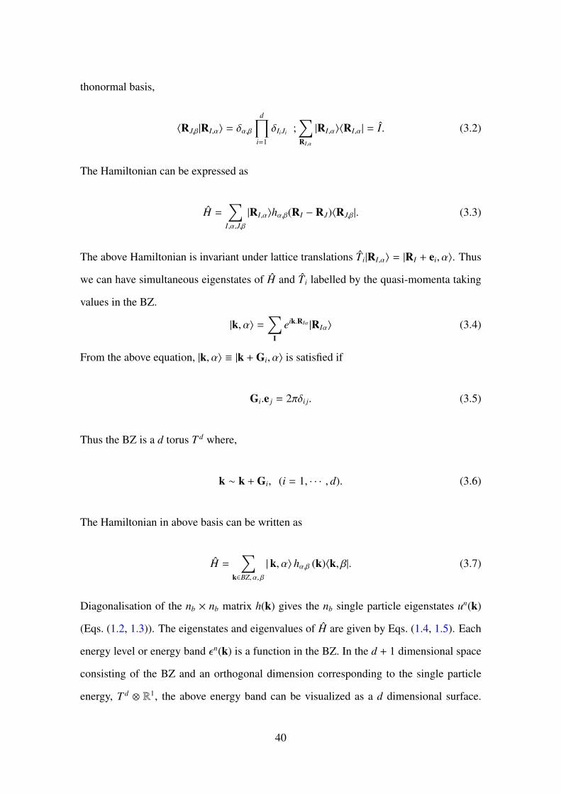
3 Quantum Geometry of Tight Binding Models and Mean Field States 39
3.1 Quantum geometry of the mean field many-body states . . . . . . . . . . 44
3.1.1 Bargmann invariants for mean field states as expectation values of
unitary operators . . . . . . . . . . . . . . . . . . . . . . . . . . 45
4 Quantum Geometry of Correlated Many-body States 49
i

4.1 Quantum distances for correlated states . . . . . . . . . . . . . . . . . . . 50
4.1.1 The exchange operators . . . . . . . . . . . . . . . . . . . . . . . 50
4.1.2 The quantum distances . . . . . . . . . . . . . . . . . . . . . . . 52
4.1.3 Satisfaction of Triangle Inequalities . . . . . . . . . . . . . . . . 54
4.1.4 Construction of the exchange operators . . . . . . . . . . . . . . 56
4.1.5 Failure in Generalisation of the Geometric Phase . . . . . . . . . 58
4.2 Conclusion . . . . . . . . . . . . . . . . . . . . . . . . . . . . . . . . . 60
5 Space of the Distances 63
5.1 Intrinsic geometry of the state . . . . . . . . . . . . . . . . . . . . . . . . 65
5.2 Extrinsic geometry of the state . . . . . . . . . . . . . . . . . . . . . . . 67
5.2.1 Fundamental results in distance geometry . . . . . . . . . . . . . 68
5.3 Distance distributions and theory of optimal transport . . . . . . . . . . . 70
5.3.1 Distance distributions . . . . . . . . . . . . . . . . . . . . . . . . 70
5.3.2 Theory of optimal transport . . . . . . . . . . . . . . . . . . . . . 71
5.4 Application to the one-dimensional t − V model . . . . . . . . . . . . . . 73
5.4.1 Physics of the model . . . . . . . . . . . . . . . . . . . . . . . . 73
5.4.2 Distance matrices at different interaction values . . . . . . . . . . 75
5.4.3 Heuristic study of the properties . . . . . . . . . . . . . . . . . . 80
5.4.4 Conclusions . . . . . . . . . . . . . . . . . . . . . . . . . . . . . 87
6 Euclidean Embedding of the Distances 91
6.1 Embedding of mean field states . . . . . . . . . . . . . . . . . . . . . . . 92
6.2 Isometric Euclidean embedding . . . . . . . . . . . . . . . . . . . . . . . 94
6.2.1 Isometric embedding of the distance matrix of t − V model . . . . 95
6.3 Approximate Euclidean Embedding . . . . . . . . . . . . . . . . . . . . 99
6.3.1 Truncation of Gram matrix spectrum with error estimate . . . . . 99
6.3.2 Average distortion . . . . . . . . . . . . . . . . . . . . . . . . . . 101
7 Wasserstein Distances 103
ii

7.1 Theory of Optimal Transport . . . . . . . . . . . . . . . . . . . . . . . . 104
7.1.1 Basic definitions . . . . . . . . . . . . . . . . . . . . . . . . . . 105
7.2 Wasserstein distances defined from the quantum distances . . . . . . . . . 107
7.2.1 Physical Interpretation . . . . . . . . . . . . . . . . . . . . . . . 107
7.2.2 Results for the t-V model . . . . . . . . . . . . . . . . . . . . . . 109
7.3 Wasserstein distances defined from the Euclidean distances . . . . . . . . 114
7.4 Approximate Euclidean embedding of the Wasserstein distances . . . . . 117
7.4.1 Approximate embedding of W by truncation . . . . . . . . . . . . 118
7.4.2 Approximate embedding of W by distortion . . . . . . . . . . . . 118
7.4.3 “Shapes” of the many-body correlated state . . . . . . . . . . . . 119
7.4.4 Conclusions . . . . . . . . . . . . . . . . . . . . . . . . . . . . . 121
8 Wasserstein Barycenter 123
8.1 Basic definition and computation . . . . . . . . . . . . . . . . . . . . . . 124
8.2 Results for the t − V model . . . . . . . . . . . . . . . . . . . . . . . . . 127
9 Ollivier-Ricci Curvature 131
9.1 Results for the t − V model . . . . . . . . . . . . . . . . . . . . . . . . . 134
10 Summary and Outlook 137
10.1 Future plans . . . . . . . . . . . . . . . . . . . . . . . . . . . . . . . . . 140
A Appendix 143
A.1 Quantum distances of general mean field states . . . . . . . . . . . . . . 143
A.1.1 The quantum distance matrix . . . . . . . . . . . . . . . . . . . . 144
A.2 The classical Ptolemy problem for α = 2 . . . . . . . . . . . . . . . . . . 146
A.3 Optimal transport problem at the extreme interaction limits . . . . . . . . 148
A.3.1 V = 0 . . . . . . . . . . . . . . . . . . . . . . . . . . . . . . . . 148
A.3.2 V = ∞ . . . . . . . . . . . . . . . . . . . . . . . . . . . . . . . . 150
Bibliography 153
iii

List of Figures
2.1 In t−t� model mapping from the BZ to the Bloch sphere for t = 1, t� = 0.3,
for a lattice of 1000 sites . . . . . . . . . . . . . . . . . . . . . . . . . . 31
2.2 In t−t� model mapping from the BZ to the Bloch sphere for t = 1, t� = 3.0,
for a lattice of 1000 sites . . . . . . . . . . . . . . . . . . . . . . . . . . 32
2.3 In the honeycomb lattice mapping from the BZ to the Bloch sphere for
t = 1,V = 3.0, for a 300 × 300 square lattice . . . . . . . . . . . . . . . . 34
2.4 In the honeycomb lattice mapping from the BZ to the Bloch sphere for
t = 1,V = 0.3, for a 300 × 300 square lattice . . . . . . . . . . . . . . . . 34
2.5 Triangulation of a four-vertex loop in the projective Hilbert space. . . . . 37
3.1 Schematic figure for understanding the quantization of the integral of
the Berry curvature of a band over the full BZ in two-dimensional tight-
binding models. . . . . . . . . . . . . . . . . . . . . . . . . . . . . . . . 43
4.1 Schematic figure for the action of exchange operators in the projective
Hilbert space. . . . . . . . . . . . . . . . . . . . . . . . . . . . . . . . . 53
4.2 The schematic figure for a tetrahedron in the projective Hilbert space be-
ing mapped to a new triangle in the spectral parameter space. . . . . . . . 54
4.3 Algorithm for verifying the satisfaction of additive law. . . . . . . . . . . 59
4.4 The probability distribution P(θ) of obtaining a deviation Δφ from the
additive law in the range, θ ≤ Δφ ≤ θ + δθ, where δθ = π100 . . . . . . . . . 60
5.1 The schematic representation of the graph of a 9-site system. . . . . . . . 65
iv

5.2 Schematic figure for the two points seperated by distance 1 as obtained
from the distance matrix. . . . . . . . . . . . . . . . . . . . . . . . . . . 77
5.3 Distance matrices obtained from numerical computation for different in-
teraction strengths . . . . . . . . . . . . . . . . . . . . . . . . . . . . . . 78
5.4 Distance d(−π, k) between k = −π and the other k modes in the Brillouin
zone (BZ) for different values of the interaction strength V . . . . . . . . . 80
5.5 Difference of distances across the Fermi point, δ and Δ: the derivative of
the distance d(−π, k) at k = −π/2, for different system sizes. . . . . . . . . 81
5.6 The edges {ei}, i = 1, 2, 3, of the Particle Triangles as a function of inter-
action strength. . . . . . . . . . . . . . . . . . . . . . . . . . . . . . . . 82
5.7 Particle triangles for different values of interaction strength . . . . . . . . 82
5.8 The edges {ei}, i = 1, 2, 3, of the particle-hole triangles as a function of
interaction strength. . . . . . . . . . . . . . . . . . . . . . . . . . . . . . 82
5.9 Particle-hole triangles for different values of interaction strength . . . . . 83
5.10 The edges {ei}, i = 1, 2, 3, of the particle-hole triangles with the special
edge (i, i + L2 ) as a function of interaction strength. . . . . . . . . . . . . . 83
5.11 The particle-hole triangles with the edge (i, i+ L2 ) ≡ e1, for different values
of interactions. . . . . . . . . . . . . . . . . . . . . . . . . . . . . . . . . 84
5.12 Distances between kre f = −π2 and other modes kn ∈ FS , as a function of
the seperation between them in the BZ, Δkre f = kn − kre f , for V = 1. . . . . 84
5.13 Nearest Neighbour Distance for different interaction strength V , over half
the BZ. . . . . . . . . . . . . . . . . . . . . . . . . . . . . . . . . . . . . 85
5.14 Schematic representations on the unit circle for different values of the
interaction V . . . . . . . . . . . . . . . . . . . . . . . . . . . . . . . . . 86
5.15 The schematic representation of the graph of ground state of the t−V model. 88
6.1 Algorithm for isometric embedding of quantum distances. . . . . . . . . . 94
6.2 Volume of the L simplex as a function of the interaction, for 18 sites. . . . 98
v

6.3 Truncation error for keeping first few (1-3) eigenvalues of G as a function
of V . . . . . . . . . . . . . . . . . . . . . . . . . . . . . . . . . . . . . . 100
6.4 Average distortion for approximate embedding of D in lower dimensions
as a function of interaction strength. . . . . . . . . . . . . . . . . . . . . 102
7.1 Algorithm for computation of the Wasserstein distance starting from the
matrix of quantum distances D . . . . . . . . . . . . . . . . . . . . . . . 105
7.2 Schematic figure depicting the distribution functions, mi( j) (i, j = 1, ..., L),
defined at each point in the BZ for the two regimes of interaction, for 18
sites. . . . . . . . . . . . . . . . . . . . . . . . . . . . . . . . . . . . . . 110
7.3 W (2)∞ as a function of the inverse system size L−1 for system sizes L = 10−28.110
7.4 Squared Wasserstein Distance matrices W (2)(mi,mj) for L = 18, obtained
from numerical computation for different values of interaction strength. . 112
7.5 The converged optimal joint probability distribution π∗i j, for L = 18, ob-
tained from numerical linear programming for different values of interac-
tion strength. . . . . . . . . . . . . . . . . . . . . . . . . . . . . . . . . . 113
7.6 Squared Wasserstein distances between distributions defined at quasi-momenta
modes inside the Fermi sea, W (2)(mkin ,mkin), as a function of the interaction
strength V , for system sizes L = 10, 14, 18. . . . . . . . . . . . . . . . . . 113
7.7 Squared Wasserstein distances between distributions defined at quasi-momenta
modes inside the Fermi sea and those outside it, W (2)(mkin ,mkout), as a func-
tion of the interaction strength V for system sizes L = 10, 14, 18. . . . . . 114
7.8 Squared Wasserstein Distance matrices W (2)E (mi,mj) for L = 18, obtained
from numerical computation for different values of interaction strength. . 115
7.9 Squared Wasserstein distances between distributions defined at quasi-momenta
modes inside the Fermi sea, W (2)E (mkin ,mkin), as a function of the interaction
strength V , for system sizes L = 10, 14, 18. . . . . . . . . . . . . . . . . . 116
vi

7.10 Squared Wasserstein distance between distributions defined at quasi-momenta
modes inside the Fermi sea and those outside it, W (2)E (mkin ,mkout), as a func-
tion of the interaction strength V , for system sizes L = 10, 14, 18. . . . . . 117
7.11 Truncation error for keeping first few (1−3) eigenvalues of G as a function
of the interaction strength, for approximate embedding of W. . . . . . . . 118
7.12 Average distortion for approximate embedding of W as a function of the
interaction strength. . . . . . . . . . . . . . . . . . . . . . . . . . . . . . 119
7.13 The embedded vectors of the Wasserstein distance in three dimensions. . . 120
8.1 The barycenter m∗(k) defined over the BZ, k ∈ [−π, π), for different inter-
action values. . . . . . . . . . . . . . . . . . . . . . . . . . . . . . . . . 128
8.2 Average squared Wasserstein distance between the distribution functions
and the barycenter as a function of the interaction strength, for different
system sizes. . . . . . . . . . . . . . . . . . . . . . . . . . . . . . . . . . 128
8.3 Average squared Wasserstein distance between the distribution functions
and the barycenter at the extreme interaction limit, V = ∞ for system
sizes L = 10 − 100, as a function of the inverse of system size. . . . . . . 129
9.1 Schematic figure for understanding the generalisation of the Ricci curva-
ture to the discrete setting as proposed by Ollivier. . . . . . . . . . . . . . 132
9.2 Curvatures for the nearest neighbour edges (k, k + 1) over half the BZ, for
different interaction strengths. . . . . . . . . . . . . . . . . . . . . . . . . 134
9.3 Curvatures for both type of edges e1 and e2 as function of interaction
strength V . . . . . . . . . . . . . . . . . . . . . . . . . . . . . . . . . . . 135
9.4 Scalar Curvature as a function of the quasi-momenta modes representing
vertices of the graph. . . . . . . . . . . . . . . . . . . . . . . . . . . . . 136
vii

viii

Synopsis
Introduction
The discovery of the quantum Hall effect has initiated a foray of research activities in-
vestigating ideas of geometry to understand and characterise the phases of many electron
systems in the last few decades. The relevance of quantum geometry for condensed matter
systems was first brought into limelight when Thouless, Kohmoto, Nightingale and den
Njis in a pioneering paper [1] pointed out that for non interacting electrons in a magnetic
field and a periodic potential, if the quasi-momenta were chosen as the parameters param-
eterising the single particle states, then the quantised Hall conductivity could be identified
with the Chern invariant which is the integral of the Berry curvature (BC) over the Bril-
louin zone (BZ). The anomalous component of the fermion velocity, perpendicular to the
acceleration as discovered by Karplus and Luttinger [3] has been found to be a physical
manifestation of the BC [4, 5, 16]. Haldane further showed in his famous work [5] that the
BC can occur even without an external magnetic field if time-reversal symmetry is bro-
ken. This leads to topological Fermi liquids and Chern insulators. The quantum metric
was shown to provide a natural variational parameter for anisotropic fractional quantum
Hall states [7].
Another deeply interesting direction of investigation of quantum geometry in condensed
matter system over the past few decades has been the the geometric theory of the insulat-
ing state [8]. In 1964, in his milestone paper [9], Walter Kohn proposed the idea that all
1

metal to insulator transitions, including strongly correlated interacting solids, are charac-
terised by the structural transformation of the ground state in the insulating phase. This
idea was substantiated years later by developments in quantum geometry [10, 11, 12, 13].
After the development of the modern theory of polarisation in 1993 [14], the polarisation
was connected to the Berry phase [10, 11]. In 1999 Resta and Sorella provided the def-
inition of many-electron localisation deeply rooted in theory of polarisation [12]. These
ideas were generalised and put on a firmer foundation by the work of Souza, Wilkens and
Martin [13] who used a generating function approach to provide expressions for polarisa-
tion and localisation length in terms of the centre of mass of the many-body wavefunction.
The organisation of the electron in the ground state in the insulating phase as proposed
by Kohn was captured by the second moment of the pair correlation function, called the
localisation tensor, which was identified to be the integral of a quantum metric over the
Brillouin Zone (BZ)[15] and found to be finite in the insulating phase and divergent in
the metallic phase [12, 13]. Thus, quantum geometry has thrown new light on the the-
ory of quantum phase transitions by characterising the phases of the many-body system
beyond the Landau theory of complete characterisation of the many-body state (and thus
the phases of the system) by its symmetries.
The inner product of the Hilbert space, which is the basis of the physical interpretation of
states, naturally defines a distance between two states and a geometric phase associated
with three states [2]. If there is a subspace of the Hilbert space, parameterised by a set
of variables, such that the distances and geometric phases are smooth functions of the
parameters, then they define a quantum metric and the so called Berry curvature (BC) in
the parameter space [23, 24]. In all the works discussed above, the quantum distances
between two quasi-momenta, the geometric phase associated with three quasi-momenta
and the corresponding quantum metric and BC on the BZ is defined in terms of single-
particle states and used to characterize the quantum geometry of mean-field states. The
quantum geometry, namely, quantum distances and geometric phases in terms of physical
parameters such as the quasi-momenta, has not been formulated beyond the mean field
2

many-body wavefunctions, until now.
In this thesis I have looked into generalizations of the study of quantum geometry for
correlated many-body wave functions. When generalising to correlated systems, global
quantities like the integral of the BC over the BZ (the Chern invariant) and the inte-
gral of the quantum metric over the BZ (the localization tensor) can be defined in terms
of the response of the system to changes in the boundary conditions [16]. To define
local quantities, namely the quantum distance between two quasi-momenta and the ge-
ometric phase associated with three quasi-momenta, one approach has been to define
these quantities in terms of the zero frequency limit of the Euclidean Green’s function
[17, 18, 19, 20, 21, 22].
In this thesis, a new formalism is introduced to obtain the induced quantum distance on the
space of physical parameters such as the quasi-momenta [25], where the quantum distance
for the correlated system is defined in terms of the static correlation functions and is
purely a ground state property, in contrast to the previous Green’s function approach [17,
18, 19, 20, 21, 22]. This formalism has been applied to the simple but non-trivial model
of correlated fermions with nearest-neighbour repulsion on a one-dimensional lattice, the
so called one-dimensional t − V model, at half-filling [26, 27]. The distance matrix or
the matrix of the quantum distances in the space of the quasi-momenta is then computed
numerically using exact diagonalization and the above distance matrix is studied in the
context of the metal-insulator transition observed in the above model. This thesis further
pursues the question: what geometric quantity constructed from the above distance matrix
captures the metal-insulator transition [29] brought about by strong electron correlations?
We seek an answer by analysing the intrinsic and extrinsic geometries of the correlated
many-body state. Finally, the thesis looks into the characterisation of the above Mott
transition by a detailed analysis of optimal transport theory in the context of the quantum
geometry of the correlated many-body state [30].
3

Quantum geometry of correlated many-body states
In our work [25] we have proposed, for any many-body state, a definition of the quantum
distance between physical parameters, such as the quasi-momenta, in terms of static cor-
relation functions.
The building blocks of many body states are single-particle states. A complete set of
single-particle states can be labeled by some set of parameters that we refer to as the
spectral parameters. The spectral parameters are completely general: they could be quasi-
momenta in periodic systems, positions labelling Wannier orbitals, parameters labelling
the eigenfunctions of some confining potential like in a quantum dot or an optical trap.
Our proposed definition of quantum distances on the space of spectral parameters is in
terms of the expectation value of certain operators that we call the exchange operators.
The wavefunction, in principle, is completely characterised in terms of correlation func-
tions. The exchange operator can be written in terms of the fermion creation and annihila-
tion operators and thus the distances can be written in terms of static correlation functions.
For one-band models these are the four-point corrrelation functions.
Our definition of the quantum distance satisfies all the basic properties of a distance in-
cluding triangle inequalities (proved using Ptolemy inequality [31]) and when applied to
the mean field states it reduces to the standard definition in terms of single-particle states.
Thus, our formalism provides a geometric characterisation of the correlated many-body
state. Moreover, since our definition of the quantum distances is in terms of the expecta-
tion values of the exchange operators, it is a purely kinematic one. As a consequence, if
the state being investigated is the ground state of a system, then the geometry defined is
manifestly a ground state property.
We apply our definition to the time-reversal and parity invariant one-dimensional t − V
model where we can concentrate on the quantum distances because we do not expect any
geometric phase effects. The spectral parameters are choosen to be the quasi-momenta.
The distance matrices at strong coupling have been studied analytically and the metal-
4

insulator transition is studied by heuristic analysis of the properties of the numerical dis-
tance matrices obtained by exact diagonalization for different values of the interaction
strength V . The finite system that we are studying does not have a phase transition, but
only a crossover from the metallic to the insulating regime as V is increased. We observe
that the metallic regime is characterized by a clustering of the distances, either very small
or close to 1. It also shows signals of sharp Fermi points. As V increases the distances
spread and the Fermi points are washed out.
We have illustrated this behaviour in three ways.
• By examining the distances from a fixed point (chosen to be k = −π) to all the
others. This shows very sharp changes at the Fermi points at low V , which smoothen
out at large V .
• By examining the nearest-neighbour distances and constructing a representation of
these on a unit circle. This representation clearly shows clustering at small V , which
gets washed out at large V .
• By examining the triangles formed by the distances between three quasi momenta.
The triangles are of two types, both have finite areas in the insulating regime, which
drastically reduce in the metallic regime.
In all three cases discussed above the crossover happens around V = 2 − 4. Since pre-
vious studies [28] have established that the metal-insulator transition occurs at V = 2,
we conclude that the “clustering-declustering" feature that we observe in the distance
matrix is indeed characterizing the metal-insulator crossover. Our formalism yields non-
trivial results even for partially filled single band systems. Thus, unlike the single particle
formalism, it is capable of probing the quantum geometry of metallic phases as well as
insulating ones.
5

Intrinsic and extrinsic geometries of correlated many-body
states
In our work [29], which is sequel to the previous work [25], we attempt to find ways to
characterize the quantum geometry of many-fermion states in terms of its distance matrix.
Although we do not have a general answer, we compute the different geometric quantities
that characterize the ground state of the one dimensional t − V model, which exhibits a
transition from metallic Luttinger liquid to a CDW insulator at V/t = 2. We then analyse
how they differ in the two regimes.
We first explored an intrinsic geometry approach and studied a discrete notion of the in-
trinsic curvature. We studied finite size systems using exact diagonalization where the
quasi-momenta are discrete and finite and therefore techniques of discrete geometry are
needed to study the system. We used the defintion of the curvature in a discrete set-
ting as proposed by Ollivier [32, 33], called the Ollivier-Ricci Curvature. To compute the
Ollivier-Ricci curvature we need to compute a new distance function on the above discrete
point set of the BZ called the Wasserstein distance, which is obtained from the matrix of
the quantum distances by applying the mathematical theory of optimal transport [34] and
computed using the standard techniques of linear programming. The metallic regime is
characterised by non-uniform curvature, which sharply changes around the Fermi point,
while the insulating regime is found to be homogenous, characterised by uniform curva-
tures. Thus, the Ollivier Ricci curvature is found to be distinctly different in both phases
and is able to capture the metal-insulator transition.
The extrinsic geometry of the state is studied by analysing the exact and approximate em-
bedding of the distance matrix in Euclidean spaces [35, 36, 37, 40, 38, 39]. We show that
the distance matrices of mean-field states can always be embedded in a finite-dimensional
Euclidean space. The analytic calculations for exact embedding at strong coupling re-
veals that the isometric embedding of the distance matrix corresponds to an embedding
6

dimension which scales as the system size and hence is not finite in the thermodynamic
limit. By contrast, for the metal at V = 0, the distance matrix can be isometrically em-
bedded in one dimension. For the distance matrices obtained numerically for interaction
values V > 0, the exact embedding reveals the same result as that in the latter case. So,
for correlated states, in contrast to the mean-field states, the dimension of embedding Eu-
clidean space for the isometric embedding of the distance matrix diverges as the system
size. Using tools of approximate embedding [40, 38, 39], we showed that the distance
matrix however can be embedded in a finite dimensional Euclidean space with small error
or average distortion in the metallic regime. This is not possible in the insulating regime.
We also look at the Euclidean embedding of the Wasserstein distance matrix and we find
that it can be approximately embedded in a one dimensional space in the metallic regime.
Further, well within the insulating regime, it can be embedded in a finite-dimensional Eu-
clidean space with relatively small error and average distortion. Thus, the approximate
embedding sharply characterises the metal-insulator transition. Moreover, it can be used
to visualise the embedding in the metallic as well as insulating regimes by looking at the
embedded vectors (in three or lower dimension). Thus, the approximate embedding of
the Wasserstein distance seems to provide a method to obtain an approximate smooth sur-
face in a finite dimensional Euclidean space for correlated states, which we have further
illustrated by presenting the shapes given by the vector configurations obtained by low
average distortion in both the regimes.
An intriguing fact from the above findings is that the approximate embedding of the
Wasserstein distance matrix seems to be more physically revealing than those of the dis-
tance matrix, although it apparently seemed to contain no information about the state.
Thus, the Wasserstein distance and the underlying optimal transport theory needs a deeper
investigation in the context of the quantum geometry of correlated many-body states.
7

Study of quantum geometry of correlated states using the
theory of optimal transport
This work [30] completes our sequence of three papers on a new approach to quantum
geometry of strongly correlated fermionic systems. We address the question: what geo-
metric quantity constructed from the above quantum distance matrix can provide a better
characterisation of the correlated many-body state and thus the phases of the system?
Our proposed definition of quantum distances on the space of spectral parameters is in
terms of the expectation value of certain operators that we call the exchange operators.
The spectral parameters can be labelled by an integer, i = 1, ..., L. Starting from a general
many-particle state |Ψ� we define a set of states, |(i, j)�, associated with a (unordered) pair
of spectral parameters (i, j) and obtained by the action of the exchange operators, Ei j ,
|(i, j)� ≡ Ei j|Ψ�.
The states |(i, j)� span a subset of the many-particle Hilbert space which we call the geo-
metric Hilbert space (GHS) and denote by Hg . The matrix of quantum distances between
the spectral parameters (i, j), d(i, j) is defined in terms of the Hilbert-Schmidt distance in
Hg .
d(i, j)2 = 1 − |�Ψ|(i, j)�|2 (1)
We analyse the above distance matrix in terms of distance distributions defined at each
point in the BZ, mi( j),
mi( j) ≡ d(i, j)�L
j=1 d(i, j). (2)
We then look for a notion of distance between any two distributions mi and mj, by applying
the mathematical theory of optimal transport [34], which gives a definition for the distance
8

between any two distributions mi and mj as,
W2(mi,mj) = infπ
L�
k,l=1
d2(k, l)πi j(k, l). (3)
Where πi j(k, l) is a joint distribution whose left marginal is mi and right marginal is mj
and W2(mi,mj) is the so called Wasserstein distance. Finding the above distance involves
finding an optimal joint distribution function π∗i j(k, l) which minimises the sum defined
on the RHS in Eq. 3. Computation of the Wasserstein distance from the given distance
matrix is done numerically by linear programming.
We define a mixed state obtained from the optimal joint distribution π∗i j(k, l),
ρ(π∗i j) ≡�
k,l
π∗i j(k, l)ρkl, (4)
where the pure state density matrices, ρi j, i > j and ρ0 are
ρi j ≡ |(i, j)��(i, j)|, ρ0 ≡ |Ψ��Ψ|.
The above distance in Eq. 3 can then be rewritten as
W2(mi,mj) = (1 − Trρ0ρ(π∗i j)) =�12
Tr(ρ0 − ρ(π∗i j))2 +
12
(1 − Trρ2(π∗i j))�. (5)
Thus the Wasserstein distance can be expessed in terms of quantities defined on Hg.
From numerical and analytic results (at strong coupling), we find that the Wasserstein
distance in the insulating phase becomes zero in the thermodynamic limit and is non-zero
in the metallic phase. So this distance provides a sharp geometric characterisation of the
state and thus the phases of a system.
9
Starting from the L distance distribution functions {mi}, we now ask for some appropriate
average distribution function representing the configuration of the above L distributions.
This can be done by further application of the optimal transport theory, by minimisation
of the following function,
J(ρ∗) =1L
L�
i=1
Wγ(mi, ρ∗).
Here ρ∗ is a single distribution function called the barycenter and J(ρ∗) is the average
Wasserstein distance between ρ∗ and the L starting distance distributions. The barycen-
ter is found to be a function on the BZ that can potentially sharply distinguish between
the metallic and insulating phases. We have also identified a single parameter, the aver-
age Wasserstien distance between the barycenter and all the distance distributions, which
sharply distinguishes between the metallic and insulating phases.
10

Bibliography
[1] D. J. Thouless, M. Kohmoto, M. P. Nightingale, and M. den Nijs, Phys. Rev. Lett.,
vol. 49, p. 405, (1982).
[2] N. Mukunda and R. Simon, Annals of Physics, vol. 228, p. 205, (1993).
[3] R. Karplus and J. M. Luttinger, Phys. Rev. 95, 1154 (1954).
[4] G. Sundaram and Q. Niu Physical Review B, vol. 59, no. 23, p. 14915, (1999).
[5] F. Haldane Physical review letters, vol. 93, no. 20, p. 206602, (2004).
[6] D. Xiao, M.-C. Chang, and Q. Niu, Rev. Mod. Phys. 82, 1959 (2010).
[7] F. D. M. Haldane, “Topology and geometry in quantum condensed matter,” 2012.
PCCM/PCTS Summer School, July 23-26, 2012.
[8] R. Resta The European Physical Journal B-Condensed Matter and Complex Sys-
tems, vol. 79, no. 2, p. 121, (2011).
[9] Walter Kohn, Phys. Rev., vol. 133, no. 1A, p. A171–A181, (1964).
[10] R. Resta, Berry Phase in Electronic Wave Functions,
[11] R. Resta, Phys. Rev. Lett., vol. 80, p. 1800, (1998).
[12] R. Resta and Sandro Sorella, Phys. Rev. Lett., vol. 82, p. 370, (1999).
[13] I. Souza, T. Wilkens, and R. M. Martin, Phys. Rev. B, vol. 62, p. 1666, (2000).
11

[14] R. D. King-Smith and David Vanderbilt, Phys. Rev. B(R), vol. 47, p. 1651, (1993).
[15] C. Sgiarovello, M. Peressi, and R. Resta, Phys. Rev. B, vol. 64, p. 115202, (2001).
[16] G. Sundaram and Q. Niu, Phys. Rev. B, vol. 59, p. 14915, (1999).
[17] Z. Wang, X.-L. Qi, and S.-C. Zhang, Phys. Rev. Lett., vol. 105, p. 256803, (2010).
[18] Z. Wang and S.-C. Zhang, Phys. Rev. X, vol. 2, p. 031008, (2012).
[19] L. Wang, X. Dai, and X. C. Xie, Phys. Rev. B, vol. 84, p. 205116, (2011).
[20] V. Gurarie, Phys. Rev. B, vol. 83, p. 085426, (2011).
[21] K.-T. Chen and P. A. Lee, Phys. Rev. B, vol. 84, p. 205137, (2011).
[22] Z. Wang, X.-L. Qi, and S.-C. Zhang, Phys. Rev. B, vol. 85, p. 165126, (2012).
[23] P. V. Sriluckshmy, A. Mishra, S. R. Hassan and R. Shankar, Phys. Rev. B 89,
vol. 045105, (2014).
[24] J. P. L. Faye, D. SÃl’nÃl’chal, and S. R. Hassan, Phys. Rev.B, vo. 89, p. 115130,
(2014).
[25] S. R. Hassan, R. Shankar, and Ankita Chakrabarti, Phys. Rev. B, vol. 98, p. 235134,
(2018).
[26] C. N. Yang and C. P. Yang, Phys. Rev., vol. 150, p. 321, (1966).
[27] M. A. Cazalilla, R. Citro, T. Giamarchi, E. Orignac, and M. Rigol, Rev. Mod. Phys.,
vol. 83, p. 1405, (2011).
[28] R. Shankar, International Journal of Modern Physics B, vol. 04, p. 2371, (1990).
[29] Ankita Chakrabarti, S. R. Hassan and R. Shankar, Phys. Rev. B, vol. 99, p. 085138,
(2019).
12

[30] “Metals,insulators and the theory of optimal transport”,
S. R. Hassan, Ankita Chakrabarti and R. Shankar.
Manuscript under preparation and to be submitted soon.
[31] I. J. Schoenberg, Ann. Math., vol. 41, p. 715, (1940).
[32] Y. Ollivier, Journal of Functional Analysis, vol. 256, p. 810, (2009).
[33] Y. Ollivier, Probabilistic Approach to Geometry, Vol. 57 (Mathematical Society of
Japan, 2010).
[34] C. Villani, Optimal Transport: Old and New , 2009th ed., Grundlehren der mathe-
matischen Wissenschaften (Springer, 2008).
[35] B. Loisel and P. Romon, Axioms, vol. 3, p. 119, (2014).
[36] I. J. Schoenberg, Annals of Mathematics 38, 787 (1937).
[37] L. Liberti and C. Lavor, International Transactions in Op- erational Research,
vol. 23, (2015).
[38] P. Indyk and J. Matousek, in Handbook of Discrete and Computational Geometry
(CRC Press, 2004), p. 177-196.
[39] Y. Rabinovich, Proceedings of the Thirty-fifth Annual ACM Symposium on Theory
of Computing, STOC ’03, 456 (2003).
[40] D. B. Skillicorn, Understanding Complex Datasets: Data Mining with Matrix De-
compositions (CRC press, 2008), p. 9-87.
13

14

Chapter 1
Introduction
The geometrical aspect of quantum mechanics has been a subject of active research ever
since Berry’s discovery[1] of the geometric phase in 1984. The Berry phase is the gauge-
invariant total phase picked up by the quantum state along a closed path. It is a geometrical
object, which can be expressed in terms of local geometric observables in the space of
variables parameterising the quantum states. It can be expressed as a line integral over a
loop in parameter space or as a surface integral of the Berry curvature over the surface
having the loop as a boundary.
Why should condensed matter physicists be bothered with quantum geometry?
Because the physical manifestations of the geometry of the quantum states in condensed
matter systems has been spectacular.
Quantum geometry first captured the attention of condensed matter physicists with the
pathbreaking discovery of Thouless et al.[2] in the quantum Hall effect.
In two-dimensional crystals, where the Fermi energy lies in a gap between Landau lev-
els, the quantized Hall conductivity is connected to the topological invariance of energy
bands[2, 3, 4]. The transverse Hall conductivity is given by a topological invariant, the
Chern number, which is the quantized geometric phase obtained as integral multiples of
2π. It is the integral of the Berry curvature of an energy band over the full Brillouin zone.
15

Quantum geometry thus provides an explanation for the quantization of the transverse
Hall conductivity and also its robustness and insensitivity to small changes in the mate-
rial’s properties.
Haldane showed that the Hall effect can also be induced by the band structure in the
absence of magnetic field by constructing a tight-binding model on a honey-comb lattice
with zero net flux per unit cell[5]. So, non-zero Chern numbers can also be observed with-
out magnetic field if the time-reversal symmetry is broken, giving birth to the concept of
Chern insulators. An unquantized geometric phase effect observed in condensed matter
systems is the anomalous quantum Hall effect. In the study of large spontaneous Hall
current in a ferromagnet in response to an electric field, the Karplus-Luttinger anomalous
velocity[6] has been reinterpreted and identified with the Berry curvature[7, 8, 9, 10] in a
new geometrical theory.
A modern theory of polarization in electronic structure theory[11, 12] has been developed,
where the change in polarization of crystalline solids has been connected to the Berry
phase of the electronic wavefunction.
For inspecting the geometry of a quantum state we have discussed the study of the ge-
ometric phase. A complementary aspect of the study of geometry of quantum states is
the study of the quantum distances between the states (defined later in Eq (1.9)) and the
corresponding induced differential metric in the space of parameters. The integral of the
quantum metric over the parameter space, the localisation tensor, characterises the insu-
lating state in a geometrical theory[13]. The quantum metric was also shown to provide a
natural variational parameter for anisotropic fractional quantum Hall states [14].
Quantum geometry has been shown to be a natural consequence of quantum kinematics[15].
It is very powerful in characterising the phases of a system, as we found for quantum Hall
systems or for the metal-insulator transition. So the study of the geometry of the many-
body state in the study of quantum phase transitions, is indispensable.
16

1.1 Quantum geometry of non-interacting electrons
Let us investigate the quantum geometry of a system of electrons in a periodic potential,
for a perfect crystalline solid. Owing to the discrete lattice translational symmetry, the
quasi-momenta defining the Brillouin zone (BZ) is a natural choice of parameters.
The hamiltonian for a nb tight-binding model for a d dimensional lattice has the simple
form,
H =�
k∈BZ,α,β
hα,β(k)C†αkCβk. (1.1)
α, β label the nb number of orbitals. The quasi-momenta k are d dimensional vectors
k = (k1, k2, . . . kd), taking values in the BZ.
Diagonalisation of nb × nb matrix h(k) gives the single particle eigenstates,
hα,β(k)unβ(k) = �n(k)un
α(k), n = 1, · · · nb. (1.2)
⇒ h(k)un(k) = �n(k)un(k) (1.3)
The eigenstates of H are,
|nk� = unα(k)|k,α� (1.4)
H|nk� = �n(k)|nk�. (1.5)
The single particle states un(k) are parametrised by the quasi-momenta k. They sit in the
projective Hilbert space, where all states {eiφun(k)} are equivalent because the phase eiφ is
not physically measurable. All the above states of the Hilbert space differing from each
other by an arbitrary (gauge-dependent) phase factor, are representated by the density
matrix ρn(k) = un(k) (un(k))†, in the projective Hilbert space. This space is a complex
manifold CPnb−1 for the above nb level system.
Each point on the BZ has a corresponding image ρn(k) in CPnb−1, representing the nth
band . Thus each band will correspond to a surface in CPnb−1. Quantum geometry pro-
17

vides geometric characterisation of this surface in terms of the quantum distance and the
geometric phase, which we define next.
All observable physical quantities are functions on projective Hilbert space. These can
expressed in terms of the so called Bargmann invariants[16, 15, 17] which are constructed
from the inner products of the single particle states. For every band, with every ordered
sequence of m points in the Brillouin zone {k} = (k1, k2, . . . ,km), we can associate a
corresponding mth order Bargmann invariant. It is defined in terms of the density matrices
of the single particle states.
The second order Bargmann invariant is defined as,
B2(k1, k2) ≡�un†(k1)un(k2)
� �un†(k2)un(k1)
�≡ Tr ( ρn(k1)ρn(k2) ) . (1.6)
The third order Bargmann invariant is defined as,
B3(k1, k2, k3) ≡�un†(k1)un(k3)
� �un†(k3)un(k2)
� �un†(k2)un(k1)
�≡ Tr ( ρn(k1)ρn(k2)ρn(k3) ) .
(1.7)
The general mth order Bargmann invariant is associated with an ordered sequence of m
states, {un(k)} ≡ (un(k1), un(k2), . . . , un(km)). It is defined as follows,
Bm ≡ Tr ( ρn(k1)ρn(k2) . . . ρn(km) ) . (1.8)
The Bargmann invariants have a geometric interpretation in terms of quantum distances
and geometric phases[15, 17].
This allows us to define an induced distance between any two points in the Brillouin zone
and a geometric phase associated with every loop in it.
The quantum distance, d(ki, k j), is defined in terms of the second order Bargmann invari-
ant as follows:
18

d(ki, k j) ≡�
1 −�B2(ki, k j)
�α. (1.9)
The above distances satisfy all the properties of a metric for α ≥ 0.5.
The geometric phase associated with the loop {k} corresponds to the geometric phase in
the projective Hilbert space defined by the ordered sequence of states, {un(k)}. It is de-
fined in terms of the phase of the corresponding mth order Bargmann invariant defined in
Eq. (1.8).
The “loop" in question is defined as the union of the segments, (un(ki), un(ki+1)) with
un(km+1) ≡ un(k1). This identification could not have been possible if the phases of the
Bargmann invariants did not satisfy additive laws by construction. A loop can be ex-
pressed as a union of several smaller loops. The sum of the phases of the Bargmann
invariants associated with the smaller loops should match the phase of the full loop. This
is ensured by the additive law satisfied by them.
We assume that the surface corresponding to the single particle states inCPnb−1 is a smooth
surface. We can thus define a differential quantum metric in the BZ from the distance
between two infinitesimally seperated states and a geometric phase associated with in-
finitesimal loops.
So, the quantum geometry is studied in terms of the single particle states with the quasi-
momenta as the physical parameters. These states connect the BZ and the Hilbert space.
For non-interacting or mean-field cases the many-body ground state is given by the Slater
determinant constructed from the single particle states. Consequently, the geometrical
observables can be explicitly expressed in terms of the single-particle states.
19

1.2 Life in Correlated Scenario
In case of narrow bands like partially filled d and f shells, the effect of electron interactions
cannot be neglected, leading to inclusion of interaction terms in the Hamiltonian. Electron
interactions lead to interesting physical phenomena like Mott transitions, unconventional
superconductivity, to name a few. The physics of correlated electrons have fascinated
condensed matter physicists for past few decades.
However, the simplest interaction term being a quartic term, the Hamiltonian is no longer
quadratic in the Fermionic operators (like in the tight-binding models) and life becomes
complicated. For a better understanding let us have a look at the example of a simple and
popular model of correlated electrons.
The Hamiltonian for a single-orbital Hubbard model on d dimensional hypercubic lattice
of N sites is,
H = −t�
�i, j�,σ
�C†iσC jσ + H.c.
�+ U
�
i
ni↑ni↓ = Hband + HU . (1.10)
The first term corresponds to the kinetic energy due to nearest neighbour hopping and the
second term gives the onsite Coulomb repulsion, where niσ = C†iσCiσ .
The Fourier transform is defined as follows :
Ckσ =1
Nd/2
�
i
eik.riCiσ. (1.11)
The kinetic energy term is given by
Hband = −t�
k,σ
d�
i=1
{e−kia + ekia}C†kσCkσ =
�
k
�(k)C†kσCkσ (1.12)
where, �(k) = −4t�d
i=1 cos(kia). We get back the familiar form in Eq. (1.1) and studies of
Sec. (1.1) holds through.
20

However, the interaction term is quite complicated and not diagonal in the quasi-momenta:
HU =UNd
�
k
�
q
�
q1
C†k+ q
2 ↑C†
k− q2 ↓
Ck− q12 ↓Ck+ q1
2 ↑ . (1.13)
Clearly, the quasi-momentum is no longer a good quantum number. The many-body state
is complex and does not have a simple form like the Slater determinant constructed from
the single particle states.
We cannot think of a map from the Hilbert space to the BZ defined by the single-particle
states.
So how to generalize the concepts of quantum geometry studied in Sec. (1.1) for corre-
lated electrons?
This is the primary question we investigate in this thesis.
An existing approach has been to consider the parameters in the wavefunction to be a
“flux” or “twist” in the electronic Hamiltonian. The “twist” in question affects the eigen-
values and eigenvectors of the many-body quantum state depending on the chosen bound-
ary conditions[9].
The linear response of the many-body wavefunction to an infinitesimal twist and the dis-
tance between the (infinitesimally) twisted and untwisted ground states are then studied.
Souza et. al.[18] showed that the localization tensor, which characterises the insulating
state, can be written as an average over the space of twisted boundary conditions of a
metric defined on the manifold of ground states of the system with twisted boundary con-
ditions.
Note first that the space of twists is not a space of physical parameters. The second point
to note is that local geometric quantities like the quantum distances between any two
points, or the geometric phase associated with a triplet of points in the parameter space,
remain inaccessible.
Only global averaged quantities, like the integral of the Berry curvature (the Chern in-
21
variant) and the integral of the quantum metric (the localization tensor) over the space of
parameters, can be studied.
To define the local quantities, namely the induced quantum distance between two quasi-
momenta and the geometric phase associated with three quasi-momenta, there exists a
Green’s function approach [19, 20, 21, 22, 23, 24]. In this approach these quantities have
been defined in terms of the zero frequency limit of the Euclidean Green’s function.
We have proposed a new formalism to generalize the concepts of quantum geometry to
correlated many-body states.
1.3 Motivation and the spirit of our formalism
Let us begin with a question addressed by Walter Kohn long back in 1964[25]. Is the
metal-insulator transition captured by some features of the ground state alone?
The transition does not involve any change of symmetries, hence, cannot be studied with
Landau’s approach[26] of the presence or absence of long range order of local order
parameters in the ground state.
The conventional approach for band insulators has involved an analysis of the low lying
excited states of the spectrum. However, quantum Hall insulators and Chern insulators
which we discussed earlier are characterised by topological invariants. We also find in
Nature correlated Mott insulators and Anderson insulators as an effect of disorder. Can
there be some uniform way of characterising the insulating state of matter?
Kohn argued that insulating states are characterised by the fact that they are insensitive
to changes in the boundary conditions. He further stated that the class of many-body
wavefunctions that were insensitive to changes in the boundary conditions were of the
form,
Ψ(x1, . . . , xN) =∞�
M=−∞ΦM(x1, . . . , xN). (1.14)
22

In the above equation each of the functions ΦM(x1, . . . , xN) are localised around points
in the many particle configuration space, and have an exponentially small overlap in the
thermodynamic limit. His hypothesis was that the ground state wavefunction of all insu-
lating states is representated by the above form.
Finding such functions starting from the many-body wavefunction in practice is very dif-
ficult. Even starting from any known ground state wavefunction decomposing it into the
above sum (on the rhs of Eq. (1.14)) is a very difficult task. So how to quantify this
qualitative difference of organisation of electrons as proposed by Kohn?
This idea was quantitatively substantiated years later using concepts of quantum geometry
[27, 28, 29, 18, 30]. The organisation of the electron in the ground state in insulating phase
as proposed by Kohn was captured by the second moment of the pair correlation function,
called the localisation tensor[29]. It is found to be finite in insulating phase and divergent
in the metallic phase[29, 18]. Interestingly it is a geometrical object which was identified
to be the integral of quantum metric over the Brillouin Zone (BZ)[31, 32].
Much of the motivation for our work comes from these developments.
In this thesis a new formalism to generalize the concepts of quantum geometry to corre-
lated many-body states has been presented.
In this formalism we are able to define quantum distances in the space of physical vari-
ables labelling the single particle states, like the quasi-momenta. Our definition of the
quantum distances are in terms of the static correlation functions.
The many-body state as we know is completely characterized by the static correlation
functions. We have cast them in a geometrical framework pretty much in the spirit of
Resta and Sorella’s work[29], where the localization tensor, which is the second moment
of the pair correlation function, was the central geometric object.
This thesis further discusses methods to construct geometrical observables starting from
the collection of the quantum distances. We propose observables which can give geomet-
ric characterisation of the above space of distances obtained from the many-body state.
23

The formalism has been applied to a correlated model of spinless Fermions with nearest
neighbour repulsion in one dimension, the t − V model [33, 34, 35]. At half-filling, this
model exhibits a Mott transition. The efficiency of geometrical observables constructed in
our theory, in characterising the metallic and insulating phases, has been supported with
results.
1.3.1 Outline of the Chapters
In this section we summarize the content of each chapter of this thesis.
• In Chapter 2 the basic concepts of quantum geometry is discussed.
• Chapter 3 illustrates in detail the concepts developed in Chapter 2 in context of the
tight-binding models and mean field many-body states.
• Our new formalism to study the quantum geometry of correlated many-body states
has been introduced and discussed rigorously in Chapter 4. The construction of the
quantum distances has been detailed.
• The collection of quantum distances in the space of parameters labelling single-
particle states which we call the spectral parameters, gives us a new geometrical
object which is a collection of points and distances. We refer to this collection as
the space of distances and briefly introduce mathematical tools to analyse this space
of distances in Chapter 5. These tools have been analysed in much more detail in
the next chapters of the thesis.
In the later part of this chapter we apply our formalism to the t − V model. The
efficiency of the tools introduced has been illustrated with the quantum distances of
this model computed using exact diagonalization, henceforth.
• In Chapter 6 the Euclidean embedding of the quantum distances are discussed. It
is a method to study the extrinsic geometry of the correlated many-body states.
24

We ask for coordinates of a collection of points in Euclidean space, such that their
interconnecting distances are the quantum distances.
• Chapter 7 discusses the application of optimal transport theory to construct a new
metric called the Wasserstein distances, which are obtained by averaging over the
space of spectral parameter and very efficient in characterising the phases.
• Chapter 8 further discusses application of optimal transport theory to locate a single
geometric observable, the Wasserstein barycenter, which can capture the phases of
the many-body state.
• In Chapter 9 the construction of a discrete notion of Ricci curvature called the
Ollivier-Ricci curvature is discussed. The study of Ollivier-Ricci curvature reveals
intrinsic geometric properties of the many-body state.
• We finally conclude the thesis with Chapter 10.
25

26
Chapter 2
Basic Concepts of Quantum Geometry
This chapter is a brief prelude which introduces the basic concepts of quantum geometry.
The states of a quantum system belong to the projective Hilbert space as briefly discussed
in Sec. (1.1). First we familiarise ourselves with the projective Hilbert space (a terminol-
ogy encountered many times in this thesis).
The physical interpretation of quantum states introduces an inner product which induces
a natural geometry in this space. The basic geometric objects which we study are the
distances between any two states and the geometric phases associated with loops.
2.1 The projective Hilbert space
The central idea is that the phase of a normalised vector |ψ� in the Hilbert space is gauge-
dependent and arbitrary. It does not matter in physical measurements. The phase becomes
gauge-invariant and thus measurable only when we have a closed loop, which was Berry’s
important observation [1].
The collection of all vectors {eiφ|ψ�} in the Hilbert space, which is also popularly referred
to as a ray, is equivalent to just a point in the projective Hilbert space.
All physically measurable observables are independent of the gauge or choice of the phase
27

factor and are thus functions on the projective Hilbert space. This many-to-one correspon-
dence from the Hilbert space vectors to the rays in the projective Hilbert space, is defined
in terms of the density matrices. The pure state density matrices are defined as follows,
ρ(ψ) =|ψ��ψ|�ψ|ψ� . (2.1)
We can see they are in one-to-one correspondence with the rays because they cannot
differentiate eiφ|ψ� from |ψ�. They satisfy the properties,
ρ2 = ρ ,Trρ = 1. (2.2)
Let us look at the simplest example of a two-level system. Any normalized vector has the
general form
|ω, θ, φ � = eiω�cos θ2 | 0 � + eiφ sin θ2 | 1 �
�. (2.3)
In the above equation, the basis states | n �, n = 0, 1, represent an orthonormal basis.
Amongst the above three general parameters ω, θ, φ, the physical state is independent of
the phase eiω. The corresponding density matrices ρ(θ, φ) have the form,
ρ(θ, φ) = |ω, θ, φ ��ω, θ, φ |
=12
(I + n.�σ), (2.4)
where I is the identity matrix, �σ are the three Pauli spin matrices and n are the unit vectors
corresponding to points on a sphere given by
n = sin θ cos φ x + sin θ sin φ y + cos θ z. (2.5)
Thus the projective Hilbert space for a two level system is a 2-sphere, known as the Bloch
sphere.
28
For a N level system, a general vector |z� can be expanded in an orthonormal basis {|n�},n = 1...,N, as follows,
|z� =N�
n=1
(znr + izn
i )|n�. (2.6)
Corresponding density matrices are given by
ρ(z) =|z��z|�z|z� . (2.7)
The projective Hilbert space thus corresponds to a manifold called the complex projective
space CPN−1, parameterised by 2N − 2 real parameters.
2.1.1 Illustration with 2-band models
In this section, we look at two simple 2-band tight-binding models: (a) the t − t� model
in one-dimension and (b) the honeycomb lattice in two dimension, for an illustration of
the mapping from the parameter space (the BZ) to the projective Hilbert space (the Bloch
sphere in this case). The mapping is defined in terms of single particle eigenstates (as
discussed in Sec. (1.1)).
t-t� model
Consider the simple model of spinless fermions hopping on a one-dimensional lattice with
staggered hopping amplitudes t and t�. The above model is a two-orbital model where the
the hopping amplitude (within an unit cell) is t and (between two unit cells) t�. We label
the two orbitals as α and β. The Hamiltonian is
H = −t�
I
(C†IαCIβ + H.c.) − t��
�I,J�(C†IαCJβ + H.c.) = H1 + H2 (2.8)
where C†Iα(CIα) creates (annihilates) a fermion corresponding to the orbital α (in a Wannier
function basis) located at site I, specified by coordinate RI = ne1, n = 1, · · · ,N .
29

The Fourier transform can be defined as,
Ckα =1√N
�
I
eik.RICIα, (2.9)
where k = ke1, k ∈ [−π, π).Using the identity
�
I
ei(k1−k2).RI = Nδk1,k2 , (2.10)
we get
H1 = −t�
k∈BZ
(C†kαCkβ + H.c.) (2.11)
H2 = −t��
k∈BZ
(e−ik.δC†kαCkβ + eik.δC†kβCkα) (2.12)
where δ = e1.
The above calculation gives us the following 2 × 2 Hamiltonian matrix
h(k) =
0 t + t�eik
t + t�e−ik 0
. (2.13)
Diagonalising the above Hamiltonian and putting t = 1, we get the energy values for the
positive and negative energy bands as follows,
�±(k) = ±�
(1 − t�)2 + 4t�cos2(k/2) (2.14)
and the corresponding eigenstates are
u±(k) =1√2
±eiφ(k)
1
, (2.15)
φ(k) = tan−1�
t� sin k1 + t� cos k
�(2.16)
30

The corresponding density matrices are found to be
ρ±(k) =12
1 ±eiφ(k)
±e−iφ(k) 1
. (2.17)
Comparing the above with the density matrix ρ(θ, φ) for a two-level system given by
Eq. (2.4), we get the coordinates (θ, φ) on the Bloch sphere of the state corresponding to
the bands for every quasi-momenta in the BZ as the following,
θ± =π
2, φ± = φ±(k) = tan−1
� ±t� sin k1 + t� cos k
�. (2.18)
Therefore, the states always lie on the equator. There are two cases, t > t� and t < t�.
−3 −2 −1 0 1 2 3
k
−4
−3
−2
−1
0
1
2
3
4
ε(k
)
+
-
Figure 2.1: The figure at the left represent the energy bands on the BZ for t = 1, t� = 0.3,for a lattice of 1000 sites. The image of the BZ on the Bloch sphere for the positive energyband for above choice of parameters is demonstrated in the figure at the right. The statesmap to an arc on the equator. The map is not one to one. The states for the negative energyband will map to the antipodal points on the Bloch sphere.
t > t� . The observations in this regime are
1. The image of the BZ on the Bloch sphere is an arc on the equator.
2. Two points in the BZ gets mapped to the same point on the Bloch sphere and the
map is not one to one.
t < t� . The observations in this regime are
31

−3 −2 −1 0 1 2 3
k
−4
−3
−2
−1
0
1
2
3
4
ε(k
)
+
-
Figure 2.2: The energy bands for t = 1, t� = 3.0, for a lattice of 1000 sites is presented atthe figure at the left. The states map to a curve on the Bloch sphere which winds aroundthe equator once, as demonstrated in the figure at the right.
1. The map is one to one, with every point having an unique image.
2. The curve in the Bloch sphere corresponding to the positive enery eigenstates winds
around the equator once.
For t = t� the energy bands touch at k = −π, the mapping to the Bloch sphere is not well
defined at this point and the hamiltonian h(k) = 0. This is a point of topological transition
for this model.
Honeycomb lattice
The honeycomb lattice is a diatomic triangular Bravais lattice, where the basis vectors are
given by
e1 =12
x +√
32
y (2.19)
e2 =12
x −√
32
y. (2.20)
Let us consider a staggered onsite potential V and next nearest neighbour hopping t of
spinless Fermions. The orbitals are labelled by α and β. The Hamiltonian is
H = −t�
�I, J�(C†IαCJβ + H.c.) + V
�
I
(C†IαCIα −C†IβCIβ) = H1 + H2 (2.21)
32

Taking the Fourier transform as defined in Eq. (2.9) and using the identity in Eq. (2.10)
we get
H1 = −t�
δi
�
k
�(1 + eik.δi)C†kαCkβ + H.c.
�(2.22)
H2 = V�
k
(C†kαCkα −C†kβCkβ) (2.23)
The position of the orbitals are given by RIk = I1e1+ I2e2+rk, k = α, β and rk = ±√
38 y for
k = α and k = β respectively. For the nearest neighbours, RJβ is given by RJβ = RIα + δi,
where δ1 = e1, δ2 = −e2. The vectors in the BZ can be written in the form
k = k1G1 + k2G2. (2.24)
{Gi} are the reciprocal lattice vectors and using Eq. (3.5) we have the following hamilto-
nian matrix,
h(k) =
V z
z∗ −V
(2.25)
z = t (1 + cos k1 + cos k2) + i t (sin k1 − sin k2) (2.26)
The energies of the bands are then given by
�±(k) = ±�| z |2 +V2 = ±�(k). (2.27)
The corresponding density matrices are found to be
ρ±(k) =12
1 ± V
�± z�
± z∗�
1 ∓ V�
. (2.28)
33

Comparing the density matrices with Eq. (2.4), the coordinates of the states corresponding
to the bands on the Bloch sphere as
θ±(k) = cos−1�
V�(k)
�(2.29)
φ±(k) = tan−1�
Im(z)Re(z)
�(2.30)
Let us look at the band surfaces in BZ ⊗ �(k) and the states on the Bloch sphere in two
different cases in Figs. (2.3, 2.4).
Figure 2.3: (a) V > t ; The figure at the left represent the energy bands on the BZ fort = 1,V = 3.0, for a 300 × 300 square lattice. The image of the BZ on the Bloch spherefor the positive energy band for above choice of parameters is demonstrated in the figureat the right. The states map to a small region around the north pole.
Figure 2.4: (b)V < t ; The figure at the left represent the energy bands on the BZ fort = 1,V = 0.3, for a 300 × 300 square lattice. The image of the BZ on the Bloch spherefor the positive energy band for above choice of parameters is demonstrated in the figureat the right. The states map to points covering the complete northern hemisphere.
When V = 0, the bands touch at the Dirac points k1, k2 = ±(2π3 ,
2π3 ) and h(k) = 0 at these
34

points. The coordinates of these points on the Bloch sphere is ill defined and the states
for all other k collapse to the equator.
2.2 Distances and geometric phases in terms of the Bargmann
invariants
For any two quantum states ψ1 and ψ2, any physically measurable quantity should be
unaffected by phase transformations of the vectors.
For example, the phase difference δ1,2 between the above states in terms of their overlap
is,
eiδ1,2 =�ψ1|ψ2�|�ψ1|ψ2�| (2.31)
δ1,2 = −Im log(�ψ1|ψ2�). (2.32)
This phase, of course, is not gauge invariant and not of any interest for physical mea-
surements. But the modulus square of the inner product of the two vectors is one such
quantity which is of physical interest. It can be expressed in terms of the density matrices
of the states as follows,
| �ψ1|ψ2� |2= Tr( ρ(ψ1)ρ(ψ2) ). (2.33)
For three physical states, ψ1,ψ2,ψ3, we can similarly propose a complex invariant,
�ψ1|ψ2��ψ2|ψ3��ψ3|ψ1� = Tr ( ρ(ψ1)ρ(ψ2)ρ(ψ3) ) , (2.34)
which was first introduced by Bargmann as a way to distinguish unitary and antiunitary
transformations[16]. Higher order generalisations give complex invariants called nth order
Bargmann invariants associated with any ordered sequence of n states,
35

{ψ} ≡ (ψ1,ψ2, . . . ,ψn), defined as,
Bn ≡ tr (ρ(ψ1)ρ(ψ2) . . . ρ(ψn)) . (2.35)
The physical observables can be expressed in terms of the Bargmann invariants. The
quantum distances and geometric phases are defined in terms of the Bargmann invariants.
2.2.1 Quantum distances
The distances between two states, D(ψ1,ψ2), are defined in terms of the second order
Bargmann invariant B2(ψ1,ψ2) which is defined in Eq. (2.33). It corresponds to the length
of the segment (ψ1,ψ2) in the projective Hilbert space and is defined to be
D(ψ1,ψ2) ≡�
1 − �B2(ψ1,ψ2)�α. (2.36)
While the above definition automatically implies,
D(ψi,ψi) = 0, (2.37)
D(ψi,ψ j) = D(ψ j,ψi). (2.38)
The Triangle inequality
D(ψi,ψ j) + D(ψ j,ψk) ≥ D(ψi,ψk) (2.39)
is satisfied for the choice α ≥ 0.5, in Eq. (2.36).
36

ψ1 ψ2
ψ4 ψ3
Figure 2.5: Triangulation of a four-vertex loop in the projective Hilbert space.
2.2.2 Geometric Phases
Mukunda and Simon identified the phase of the Bargmann invariant with the geometric
phase[15]. Let us denote the phase of the nth order Bargmann invariant by Ω(n). That is,
Bn (ψ1,ψ2, . . . ,ψn) = eiΩ(n) | Bn (ψ1,ψ2, . . . ,ψn) | . (2.40)
It follows from the definition in Eq. (2.35) that Ω(n) obeys additive law.
Let us look at a four-vertex loop in the projective Hilbert space with vertices (ψ1, ψ2, ψ3, ψ4).
From the additive property of the phases,
Ω(4)(ψ1,ψ2,ψ3,ψ4) = Ω(3)(ψ1,ψ2,ψ3) +Ω(3)(ψ1,ψ3,ψ4) (2.41)
= Ω(3)(ψ1,ψ2,ψ4) +Ω(3)(ψ2,ψ3,ψ4). (2.42)
The above additive property allows us to write the total geometric phase associated with
the four-vertex loop in the projective Hilbert space as a sum of the phases associated with
smaller triangles whose union gives the full loop and thus triangulation of the above loop
is possible. The above equations (Eqs. (2.41) and (2.42)) give us two possible triangula-
tion as demonstrated in Fig. (2.5). The total geometric phase of the four-vertex loop is
independent of the way of triangulation, as we would expect for a physically measurable
observable.
37

Conclusion. The geometric phase associated with a loop in the projective Hilbert space
defined by the ordered sequence of states {ψ}, is identified to be the phase of the nth
order Bargmann invariant: the loop under consideration can be defined as the union of the
segments (ψi,ψi+1) with ψn+1 ≡ ψ1. The above identification is possible because a loop
in the projective Hilbert space can be expressed as the union of several smaller loops:
moreover, the geometric phase associated with the full loop is given by the sum of the
phases associated with the smaller loops. This is ensured from the additive law satisfied
by the phases of the Bargmann invariants.
38

Chapter 3
Quantum Geometry of Tight Binding
Models and Mean Field States
We investigate the quantum geometry of tight binding models and mean field many-body
states in this chapter. For translationally symmetric tight binding models, the subspace
of the quantum states in the Hilbert space is parameterised by the quasi-momenta that
define the Brillouin zone (BZ). Hence, if the quantum distances and geometric phases
are smooth functions of the quasi-momenta, they define an induced infinitesimal quantum
metric and a Berry curvature (BC) in the BZ.
Let us consider nb-band tight-binding models of a d-dimensional Bravais lattice, with
each unit cell having nb orbitals centered at
RIα = RI + rα (α = 1, · · · , nb), (3.1)
where the position of each unit cell is given by, RI =�d
i=1 Iiei. Here, {ei} are the d basis
vectors.
Let |RI,α� denote the wavefunction of the orbitals. We further assume they form an or-
39
thonormal basis,
�RJ,β|RI,α� = δα,βd�
i=1
δIi Ji ;�
RI,α
|RI,α��RI,α| = I. (3.2)
The Hamiltonian can be expressed as
H =�
I,α,J,β
|RI,α�hα,β(RI − RJ)�RJ,β|. (3.3)
The above Hamiltonian is invariant under lattice translations Ti|RI,α� = |RI + ei,α�. Thus
we can have simultaneous eigenstates of H and Ti labelled by the quasi-momenta taking
values in the BZ.
|k,α� =�
I
eik.RIα |RIα� (3.4)
From the above equation, |k,α� ≡ |k +Gi,α� is satisfied if
Gi.e j = 2πδi j. (3.5)
Thus the BZ is a d torus T d where,
k ∼ k +Gi, (i = 1, · · · , d). (3.6)
The Hamiltonian in above basis can be written as
H =�
k∈BZ,α, β
| k,α� hα,β (k)�k, β|. (3.7)
Diagonalisation of the nb × nb matrix h(k) gives the nb single particle eigenstates un(k)
(Eqs. (1.2, 1.3)). The eigenstates and eigenvalues of H are given by Eqs. (1.4, 1.5). Each
energy level or energy band �n(k) is a function in the BZ. In the d + 1 dimensional space
consisting of the BZ and an orthogonal dimension corresponding to the single particle
energy, T d ⊗ R1, the above energy band can be visualized as a d dimensional surface.
40

There are nb such surfaces.
Let us now inspect the projective Hilbert space, which is CPnb−1 for the above nb level
system. The single particle states un(k) are parametrised by the quasi-momenta k in the
BZ. Each point on the BZ has a corresponding image ρn(k) = un(k) (un(k))† representing
the nth band in CPnb−1. Thus each band will correspond to a surface in CPnb−1. Quantum
geometry provides geometric characterisation of this surface in terms of the quantum
distance and the geometric phase.
For every band of states, with every ordered sequence of m points in the Brillouin zone
{k} = (k1, k2, . . . ,km), we can associate a corresponding mth order Bargmann invariant
defined in terms of the density matrices of the single particle states. This allows us to
define an induced distance between any two points in the Brillouin zone and a geometric
phase associated with every loop in it.
If the surface in CPnb−1 is a smooth surface, we can define a differential quantum metric
in the BZ from the distance between two infinitesimally seperated states and a geometric
phase associated with infinitesimal loops. Equations 2.33 and 2.36 gives the distance
between two infinitesimally seperated states corresponding to the nth band, un(k) and
un(k + dk), as follows:
d2(k, k + dk) = 1 − (Tr ( ρn(k) ρn(k + dk) ))α =d�
a,b=1
gab dka dkb (3.8)
From the properties of the density matrices,
Tr( ρ2) = Tr( ρ) = 1⇒ Tr( ρδaρ ) = 0⇒ Tr( δaρδbρ ) = −Tr( ρδaδbρ ) (3.9)
where δa ≡ δδka
. Taylor series expansion of ρn(k + dk) (upto the second order) and use of
41

Eq. (3.9) gives,
d2(k, k + dk) � 1 −�1 +
12
Tr( ρnδaδbρn )dkadkb
�α
� α
2Tr( δaρ
nδbρn ) dka dkb
⇒ gab =α
2Tr(δaρ
nδbρn). (3.10)
Now we look at the phase of a 3-vertex Bargmann invariant with the vertices at infinitesi-
mal seperation, as given by Eq. (2.34).
Ω(3)(k, k + dk1, k + dk2) = Im ln(Tr ( ρn(k) ρn(k + dk1) ρn(k + dk2 ))). (3.11)
Taylor series expansion of the RHS and use of the properties in Eq. (3.9) as before gives
Ω(3)(k, k + dk1, k + dk2) =12i
Tr ( ρn(δaρnδbρ
n − δbρnδaρ
n) ) dka dkb (3.12)
This defines an anti-symmetric tensor
Fab(k) ≡ 12i
Tr ( ρn(δaρnδbρ
n − δbρnδaρ
n )) (3.13)
Parameterising the vertices of the triangle by two parameters k(s, t), we have k(s+ds, t) =
k + dk1 and k(s, t+ dt) = k + dk2, giving us, dka1 = δskads and dka
2 = δtkadt. We can now
write Eq. (3.12) in the following form :
Ω(3)(k, k + dk1, k + dk2) = Fab (k)12
(δskaδtkb − δskbδtka) ds dt (3.14)
= Fab(k) dka ∧ dkb (3.15)
The phase of a 3-vertex Bargmann invariant is found to be an integral of a two-form over
a surface whose boundary is given by the triangle under consideration. Any closed curve
in the projective Hilbert space can be interpreted as a limit of polygons. Moreover, any
42

N vertex Bargmann invariant corresponds to a N-sided polygon in the projective Hilbert
space : this polygon can be triangulated and the total phase can be obtained by summing
over all triangles. Using the above result, we can associate a phase with every closed
curve γ in the projective Hilbert space,
Ω(γ) =�
SFab(k) dka ∧ dkb, (3.16)
where (a) S is the surface with γ as the boundary and (b) Fab(k) is called the Berry
curvature for the nth band.
Quantization The integral of the Berry curvature of a band over the full BZ in two-
dimensional tight-binding models is found to be an integral multiple of 2π and identified
to be a topological invariant, called the Chern invariant which characterises the band.
The integral of the Berry curvature on the rhs of Eq. (3.16) represents the phase of the
Bargmann invariant constructed along the boundary of the surface S . So, if we consider
two surfaces S � and S �� having the same boundary, C, the corresponding integrals could
differ from each other only by an integral multiple of 2π. So we must have,
�
S �Fab(k) dka ∧ dkb =
�
S ��Fab(k) dka ∧ dkb + 2nπ. (3.17)
Let us assume the union of S � and S �� gives a closed surface S . A schematic representation
is demonstrated in Fig. (3.1). Now we shrink C to a point. In the limiting situation when
S��
C
S�
S
S
S�
Figure 3.1: Two surfaces S � and S �� having the same boundary C. The union of S � andS �� gives the surface S . For the figure on the right, C has been shrunk to a point givingS ≡ S �.
43

S ≡ S �, the integral over S �� should vanish, giving us,
�
S �Fab(k) dka ∧ dkb = 2nπ. (3.18)
This indicates that the integral of the Berry curvature over any closed surface in the BZ
has to be an integral multiple of 2π. However, the value of n in above equation could be
zero as well.
There are two-dimensional tight-binding models like the Haldane model where the above
integral can be non-zero and changes discontinously across the topological phase transi-
tion.
3.1 Quantum geometry of the mean field many-body states
The many-body ground state in a non-interacting or mean field scenario, for the case
when the nth band is completely filled and all others completely empty, in terms of the
single-particle wavefunctions (introduced in Eq. (1.3)) is as follows,
|n� ≡�
k
�unα(k)C†kα
�|0� (3.19)
where Ckα|0� = 0. The Fermion operators satisfy the canonical anti-commutator relations
{C†k1α,Ck2β} = δk1k2δαβ, {C†k1α
,C†k2β} = 0, {Ck1α,Ck2β} = 0. (3.20)
The mean field many-body ground state in Eq. (3.19) is not labelled by the quasi-momenta,
but has a simple form in terms of the single particle states which are parametrised by the
quasi-momenta. This allows us to connect the Bargmann invariants defined in terms of
overlap of the single-particle states to the many-body ground state and thus study the in-
duced quantum distances and geometric phase in the BZ, as we shall soon find out in next
44

section.
3.1.1 Bargmann invariants for mean field states as expectation values
of unitary operators
The quantum geometry of a band, namely the quantum distances and the geometric phases
defined in terms of the second and third order Bargmann invariants in Eqs. (2.33,2.34)
respectively, can be studied in terms of the single particle states. The second order
Bargmann invariant can be written as
B2(k1, k2) =�un†(k1)un(k2)
� �un†(k2)un(k1)
�. (3.21)
Similarly the third order Bargmann invariant can be expressed as
B3(k1, k2, k3) =�un†(k1)un(k3)
� �un†(k3)un(k2)
� �un†(k2)un(k1)
�. (3.22)
The above Bargmann invariants of order two and three defined in Eqs. (3.21,3.22) can in-
terestingly also be casted as expectation values of some suitably defined unitary operators
over the mean-field many-body state.
Eq.(3.21) can also be rewritten as
B2(k1, k2) = −�0|�un†(k1)Ck1
� �un†(k2)Ck2
� �C†k1
un(k2)� �
C†k2un(k1)
�|0�. (3.23)
Let us consider an unitary operator E(k1, k2) with the following properties
E(k1, k2) | 0� = | 0� (3.24)
E(k1, k2) C†k1,αC†k2β
E†(k1, k2) = −C†k2,αC†k1β
(3.25)
45

and a two-particle state |ψ� =�C†k2
un(k2)� �
C†k1un(k1)
�|0�. It follows form Eqs. (3.24,3.25)
that
B2(k1, k2) = �ψ | E(k1, k2) |ψ�. (3.26)
Moreover, since E(k1, k2) commutes with all the other fermion creation and annihilation
operators, i.e. (Ckα,C†kα), k � k1, k2, we can write the second order Bargmann invariant
as an expectation value of this operator over the many-body groundstate |n� defined in
Eq. (3.19).
The action of the above operator E(k1, k2) on the many-body ground state |n� can be
thought of as an exchange of fermions at quasi-momenta k1 and k2. We name this operator
accordingly as the exchange operator and the second order Bargmann invariant can thus
be written as the expectation value of the exchange operator over the many-body ground
state,
B2(k1, k2) = �n | E(k1, k2) | n�. (3.27)
The operator E(k1, k2), defined in terms of the fermion creation and annhilation operators
as follows,
E(k1, k2) ≡ eπ2�nbα=1
�C†k1α
Ck2α−H.c.�
, (3.28)
does satisfy Eqs. (3.24,3.25).
The third order Bargmann invariant defined in Eq. (3.22) can be rewritten as,
B3(k1, k2, k3) = �0|�un†(k1)Ck1
� �un†(k2)Ck2
� �un†(k3)Ck3
� �C†k1
un(k3)� �
C†k3un(k2)
� �C†k2
un(k1)�|0�.
Repeating above procedure, we construct an unitary operator C(k1, k2, k3), such that,
C(k1, k2, k3)|0� = |0�,
C(k1, k2, k3)C†k3αC†k2β
C†k1γC†(k1, k2, k3) = C†k1α
C†k3βC†k2γ. (3.29)
46

Moreover, we can construct C as a product of the exchange operators,
C(k1, k2, k3) = E(k1, k3)E(k3, k2). (3.30)
The above procedure can be followed even for higher order Bargmann invariants.
The same result can be generalised for arbitrary number of filled bands just like the above
case of one completely filled band (details in the Appendix).
Therefore, we conclude that for many-body mean field states, the Bargmann invariants
can be thought of as expectation values of the exchange operator and higher order cyclic
products of the exchange operators. Thus the quantum distances and the geometric phases
can be expressed in terms of expectation values of some suitably defined unitary operator.
47

48

Chapter 4
Quantum Geometry of Correlated
Many-body States
The immediate question which arises is: how to generalize the framework of quantum
geometry discussed so far, for correlated many-body states?
The previous chapter hints at the following hypothesis. The induced quantum distance
for any general many-body state in a space of single particle quantum numbers, which
label the single particle spectrum, can be more generally defined in terms of expectation
values of suitably defined unitary operators. For the mean field states, we called them
the exchange operators. The same can perhaps also be proposed for geometric phases by
suitably defining an unitary operator. In mean field states, this operator happened to be
products of the exchange operators.
Hence, by the above scheme the study of quantum geometry of the correlated many-body
state, in a space of physical parameters (in analogy to the BZ in case of tight binding mod-
els), might indeed be possible. We can generalize the definition of the quantum distances
and geometric phases in terms of expectation values of some appropriately defined uni-
tary operator. But for this scheme to work, the distances should satisfy all the properties
of a metric and the geometric phases should satisfy the additive law. In our new formal-
49

ism, we accomplish this task: we study the quantum geometry of correlated many-body
states by proposing a valid definition of the quantum distances in the space of spectral
parameters, for a general correlated many-body state. The quantum distances are defined
in terms of expectation values of unitary operators which we call the exchange operators.
These expectation values are in fact the static correlation functions of the system. While
the geometric phases defined in terms of product of the exchange operators do not satisfy
the additive law, our scheme leaves a future possible direction of work to track down a
correct operator. We proceed with a detailed examination of the quantum distances.
4.1 Quantum distances for correlated states
We define induced quantum distances amongst the single particle spectral parameters
like the quasi-momenta which label the single particle state, by appropriately defining an
exchange operator and taking the expectation value of this operator over the many-body
state.
4.1.1 The exchange operators
The many-body state can always be written in a Fock basis expansion and the exchange
operators are defined by their action on the Fock basis having the following form
| {n}� =�
k,α
�C†kα
�nkα |0�, C†kαCkα| {n}� = nkα| {n}�. (4.1)
Here, nk,α refers to the occupation numbers of the mode (k,α) and {n} denotes the collec-
tion of all the occupation numbers. For the empty state |0�, nk,α = 0, for every k,α.
The ordering of the fermionic operators in Eq. (4.1) is very important. We label every
50

element of the set (k,α) by a unique integer m(k,α),
Cm ≡ Ckα, nm ≡ nkα. (4.2)
The ordering corresponding to each basis state is specified by a particular combination
of the nb × Ld values of m(k,α) for a d dimensional Bravais lattice with nb number of
orbitals and Ld number of unit cells,
| {n}� =nbLd�
m=1
C†m | 0�. (4.3)
The many-body state |ψ�, when expanded in the above basis has a form
|ψ� =�
{n}ψ({n}) | {n}�. (4.4)
As a generalisation of the mean field scenario the exchange operators, E(k1, k2), are de-
fined as operators that exchanges the occupation numbers of the modes at k1 and k2, i.e.,
Eα(k1, k2)| . . . , nk1α, . . . , nk2α, . . . � ≡ |.., nk2α, .., nk1α, ..�, (4.5)
E(k1, k2) ≡nb�
α=1
Eα(k1, k2). (4.6)
Some of the properties of the exchange operator which follows immediately from the
definition are,
E†(k1, k2) = E−1(k1, k2) , E†(k1, k2) = E(k1, k2)
E2(k1, k2) = I (4.7)
51

4.1.2 The quantum distances
For a general many-particle state |ψ� we define, parallel to the second order Bargmann
invariants, a new object: the expectation value of the above exchange operators
B2(k1, k2) ≡ �ψ|E(k1, k2) |ψ�. (4.8)
The induced quantum distances between k1 and k2, which is usually defined in terms of
the second order Bargmann invariant, has been defined as follows:
d(k1, k2) ≡�
1 − (�ψ|E(k1, k2)|ψ�)α. (4.9)
The above definition can give valid distances only if they satisfy all the properties of a
metric.
From Eqs. (4.5) and (4.6), it follows that,
E(k, k) = I ⇒ d(k, k) = 0 (4.10)
E(k1, k2) = E(k2, k1)⇒ d(k1, k2) = d(k2, k1). (4.11)
So the first two properties of positivity and symmetricity immediately follow.
Before looking into the proof of triangle inequalities, let us re-examine the projective
Hilbert space. The following observations are important.
Basis Expansion. A many body wavefunction of a nh level system is a point in the
complex projective space CPnh−1. We label the single particle eigen states by quantum
numbers {i}, which can be the spin, the quasi-momenta, the position labelling the Warnier
orbitals, parameters labelling the eigenfunctions of some confining potential like in a
quantum dot or an optical trap. We can expand the many-body state |Ψ� in a direct product
52

Ψ1
ΨGS
Ψ2
Ψ3E
i2 ,i3E i 1
,i 3
Ei 1,i2
Figure 4.1: Schematic figure for the action of exchange operators in the projective Hilbertspace.
basis of the single particle states,
|Ψ� =�
i1,...,iL
ci1...iL
��������������|i1 ⊗ i2... ⊗ iL�
=
nh�
j=1
C j| j�,�
j
|C j|2 = 1
.
New States. The exchange operator Eilim generates a new (normalized) state, |��, cor-
responding to an exchange of the quantum numbers il and im,
|�� = Eil,im |�.
Distance. For the space of quantum numbers {i1, i2, ..., iL} (which we refer to as the
spectral parameters), the distance d(il, im) connecting two points (il, im) is defined in terms
of the overlap of |� and |�� :
d(il, im) =�
1 − |�Ψ�|Ψ�|α
53

4.1.3 Satisfaction of Triangle Inequalities
Why are the triangle inequalities not obvious?
We need to prove that
d(i2, i3) + d(i3, i1) ≥ d(i1, i2). (4.12)
So we have three states in the projective Hilbert space generated by the action of the three
concerned exchange operators
|Ψ1� ≡ Ei2,i3 |Ψ�, |Ψ2� ≡ Ei3,i1 |Ψ�, |Ψ3� ≡ Ei1,i2 |Ψ�.
The above distances are essentially the distances between the reference many-body state
and the above three states in the projective Hilbert space defined in Eqs. (2.33,2.36),
d(i2, i3) = D(Ψ1,Ψ) (4.13)
d(i3, i1) = D(Ψ2,Ψ) (4.14)
d(i1, i2) = D(Ψ3,Ψ) (4.15)
Together, the reference many-body state and above three states form a tetrahedron as
|Ψ1�|Ψ2�|Ψ�
|Ψ3� =⇒ i1
i2
i3
Figure 4.2: The schematic figure for a tetrahedron in the projective Hilbert space beingmapped to a new triangle in the spectral parameter space. The corresponding edges aredrawn in red colour.
demonstrated in Fig. (4.2). However the triangle under question in the spectral param-
eter space formed by vertices (i1, i2, i3) with edges (d(i2, i3), d(i3, i1), d(i1, i2)) shown in
Fig. (4.2), is not a triangle in the Hilbert space.
54

The question boils down to whether the above three edges out of the six edges of the tetra-
hedron in the projective Hilbert space will always form a valid triangle. Fortunately, the
answer to the question is yes! It follows from a famous inequality in geometry attributed
to the Greek mathematician Ptolemy. Ptolemy’s inequality[36] states that the six distances
d(i, j) between any four distinct points i, j = 1, ...4 satisfies the following inequalities
d(i, j) d(k, l) + d(i, k) d( j, l) ≥ d(i, l)d( j, l). (4.16)
The above results holds in any Hilbert space [36].
Therefore, Ptolemy’s inequality implies that
D(Ψ,Ψ1) D(Ψ2,Ψ3) + D(Ψ,Ψ2) D(Ψ3,Ψ1) ≥ D(Ψ,Ψ3) D(Ψ1,Ψ2). (4.17)
We can express the distances D(Ψi,Ψ j) (where i, j = 1, 2, 3 ,and i � j) in terms of overlap
of states generated by action of the exchange operators
�Ψ1|Ψ2� = �Ψ|Ei2,i3 Ei3,i1 |Ψ�, �Ψ2|Ψ3� = �Ψ|Ei3,i1 Ei1,i2 |Ψ�, �Ψ3|Ψ1� = �Ψ|Ei1,i2 Ei2,i3 |Ψ�.
The exchange operators satisfy the following product rules,
Ei2,i3 Ei3,i1 = Ei3,i1 Ei1,i2 = Ei1,i2 Ei2,i3 . (4.18)
So the base of the tetrahedron in Fig. (4.2) is always an equilateral triangle. This implies
that
D(Ψ1,Ψ2) = D(Ψ2,Ψ3) = D(Ψ3,Ψ1). (4.19)
Using the above result, Eq. (4.17) implies the following: if D(Ψ1,Ψ2) � 0,
D(Ψ,Ψ1) + D(Ψ,Ψ2) ≥ D(Ψ,Ψ3). (4.20)
55

If D(Ψ1,Ψ2) = 0, then the three operations give the same state and we have D(Ψ,Ψ1) =
D(Ψ,Ψ2) = D(Ψ,Ψ3). Therefore, in this case, the above identity is trivially true.
Thus we have
d(i2, i3) + d(i1, i3) ≥ d(i1, i2).
Hence, the quantum distances defined in terms of the exchange operators do satisfy tri-
angle inequalities and are, therefore, valid distances. Setting α = 2 in Eq. (4.9) as our
definition of distances, the above proof reduces to the classical problem in Euclidean
space, with the standard definition of distance (details provided in Appendix).
4.1.4 Construction of the exchange operators
Let us define the following operators,
T xα(k1, k2) ≡
�C†k1α
Ck2α +C†k2αCk1α
�(4.21)
T yα(k1, k2) ≡ 1
i
�C†k1α
Ck2α −C†k2αCk1α
�(4.22)
T zα(k1, k2) ≡
�C†k1α
Ck1α −C†k2αCk2α
�. (4.23)
for which
�T xα(k1, k2)
�2=
�T yα(k1, k2)
�2=
�T zα(k1, k2)
�2= (ρα(k1) − ρα(k2))2 , (4.24)
where ρα(k) ≡ C†kαCkα. Let us consider the unitary operators
Uα(k1, k2) ≡ ei π2 T yα(k1,k2). (4.25)
The above operators satisfy the following equations
U†α(k1, k2)�C†k1α
�Uα(k1, k2) =
�C†k2α
�
U†α(k1, k2)�C†k2α
�Uα(k1, k2) = (−1)
�C†k1α
�.
56

Hence,
U†α(k1, k2)�C†k1α
�nk1α Uα(k1, k2) =�C†k2α
�nk1α
U†α(k1, k2)�C†k2α
�nk2α Uα(k1, k2) = (−1)nk2α�C†k1α
�nk2α .
Next, consider the action of U†α(k1, k2) on the two particle states |nk2α, nk1α�
U†α(k1, k2)|nk1α, nk2α� = U†α(k1, k2)�C†k1α
�nk1α�C†k2α
�nk2α |0�
= (−1)nk2α�C†k2α
�nk1α�C†k1α
�nk2α |0�
= (−1)nk2α(1−nk1α)�C†k1α
�nk1α�C†k2α
�nk2α |0�
= (−1)nk2α(1−nk1α)|nk2α, nk1α�.
Defining the following operator,
Eα(k1, k2) ≡ eiπ(ρα(k1)(1−ρα(k2)))U†α(k1, k2) (4.26)
we have the desired action of the exchange operator on the two particle states,
Eα(k1, k2)|nk1α, nk2α� = |nk2α, nk1α�. (4.27)
The same will hold through for the Fock basis but the fermionic sign needs to be handled
carefully. Let us stick to the same convention as specified by labelling the modes as per
equation 4.3. We know from the anticommutation relations of Fermion operators,�C†m
�nm�C†l
�nl= (−1)nmnl
�C†l
�nl�C†m
�nmand we accordingly define a suitable phase factor
eiπνα(k1,k2), where
να(k1, k2) ≡ (ρα(k1) + ρα(k2))m(k2,α)−1�
l=m(k1,α)+1
ρα(kl). (4.28)
So the exchange operator defined as,
Eα(k1, k2) ≡ eiπνα(k1,k2)Eα(k1, k2) (4.29)
57

exchanges the occupation numbers of the modes at k1 and k2.
Let us simplify the above expression. Expanding the operators U†α(k1, k2) and the sign
factor in the RHS of Eq. (4.26) we get,
eiπ(ρα(k1)(1−ρα(k2))) = 1 − 2 (ρα(k1)(1 − ρα(k2))) (4.30)
U†α(k1, k2) = 1 − (ρα(k1) − ρα(k2))2 + iT yα(k1, k2) (4.31)
Using the above equations we get a simpler form for Eα(k1, k2), which is
Eα(k1, k2) = 1 − (ρα(k1) − ρα(k2))2 +�C†k1α
Ck2α +C†k2αCk1α − 2ρα(k1)δk1k2
�. (4.32)
For a one-band model, considering translationally invariant states, the expression for the
expectation values of the exchange operators has the following form,
�E(k1, k2)� = 1 −��
C†k1Ck1 −C†k2
Ck2
�2�. (4.33)
4.1.5 Failure in Generalisation of the Geometric Phase
In Section 3.1.1 we looked into definitions of the Bargmann invariants of third order
as well, for the mean-field states, in terms of expectation values of operators which are
products of the exchange operators as defined in Eq. (3.30). If the generalisation of the
above definition for the geometric phases in terms of the expectation values of the unitary
operator defined as the product of the exchange operators is correct for correlated many-
body states, then we can also define the geometric phases associated with loops in the
spectral parameter.
We have tested whether generalisation of the above scheme is possible for defining the
geometric phases in case of correlated many-body states. The algorithm for a numerical
check of the satisfaction of the additive law (given by Eqs. (2.41,2.42)) is discussed in
58

Fig. (4.3).
The probability distribution P(θ) of obtaining a deviation Δφ from the additive law in
1. We consider states of a four site, one-band, spinless fermionic system athalf-filling. The occupation number basis {(nk1 , nk2 , nk3 , nk4)} is choosen, wherenki = 0, 1 ∀i ∈ [1, 4].
2. We generate N = 106 random states.
3. We compute the following quantities for each state |ψ� :
B3(k1, k2, k3) = �ψ|E(k1, k3)E(k3, k2) |ψ�= eiΩ(3)(k1,k2,k3) | �ψ|E(k1, k3)E(k3, k2) |ψ� |
B3(k1, k3, k4) = �ψ|E(k1, k4)E(k4, k3) |ψ�= eiΩ(3)(k1,k3,k4) | �ψ|E(k1, k4)E(k4, k3) |ψ� | .
4. The total phase φ is given by
φ = Ω(3)(k1, k2, k3) +Ω(3)(k1, k3, k4). (4.34)
5. Similarly we also compute φ�,
φ� = Ω(3)(k1, k2, k4) +Ω(3)(k2, k3, k4). (4.35)
6. We then compute the deviation from the additive law (as per Eqs. (2.41,2.42)),
Δφ = φ − φ� (4.36)
7. The probability distribution P(θ) of obtaining a deviation in the range,θ ≤ Δφ ≤ θ + δθ, where δθ = π
100 is then computed.
Figure 4.3: Algorithm for verifying the satisfaction of additive law.
the range, θ ≤ Δφ ≤ θ + δθ, where δθ = π100 is shown in Fig. (4.4). We find that the
probability distribution function is sharply peaked at θ = 0. But the additive law are not
neccesarily satisfied. Infact there are many violations as the probability of the additive
law being satisfied is found to be only ∼ 7%. So the proposed scheme fails for the above
choice (Eq. (4.29)) of unitary operator and we cannot define geometric phases associated
59

−4 −3 −2 −1 0 1 2 3 4
θ
0.00
0.01
0.02
0.03
0.04
0.05
0.06
0.07
P(θ
)
Figure 4.4: The probability distribution P(θ) of obtaining a deviation Δφ from the additivelaw in the range, θ ≤ Δφ ≤ θ + δθ, where δθ = π
100 .
with loops in spectral parameter space.
4.2 Conclusion
Let us stop and reflect on the findings from our new formalism to study the quantum
geometry of correlated many-body states, as we conclude this chapter.
We have been able to give a definition for induced quantum distances in the space of
physical parameters like the quasi-momenta which label the single particle states (the
spectral parameters) for the correlated many-body states just like in the case of many-
body states in a periodic potential. So now we have access to local geometric observables
even for the correlated scenario for the very first time. The spectral parameters however
could be more generally the spin, the position labelling the Warnier orbitals, parameters
labelling the eigenfunctions of some confining potential like in a quantum dot or an optical
trap as pointed out already in Sec. (4.1.2).
The proposed definition of quantum distances are in terms of expectation values of the
exchange operators. From the explicit form of the operators in Sec.(4.1.4), we know the
definition is basically in terms of the static correlation functions. In one band system
these being the four-point correlation functions as observed from Eq. (4.33), whereas for
60

multiband systems they are higher order correlation functions.
So the quantum distances can be obtained by computation of the static correlation func-
tions applying any exact or approximate technique like quantum Monte Carlo methods,
DMRG and bosonisation in one dimension, exact diagonalisation for finite systems, per-
turbation theory and so on.
Studying the geometry of the correlated state now reduces to study of the above collection
of quantum distances in spectral parameter space. We apply our formalism to the ground
state of the one-dimensional t − V model and discuss the quantum distances in the next
chapter. While application to the ground state can throw light on characterisation of the
phases of a system in terms of geometry, application to any quantum state is possible in
principle, leading to the possibility of applications in quantum dynamical systems as well.
The following chapters will elaborate in detail the tools to study the geometry of the state
in terms of the quantum distances.
61

62

Chapter 5
Space of the Distances
Our formalism introduced in the previous chapter when applied to a correlated system
gives a set of distances {d(ki, k j)}, between points in the spectral parameter space {ki} ∈ K,
which are basically quantum numbers labelling the single particle states. Therefore, by
computing the static correlation functions applying any exact or approximate technique
(e.g. quantum Monte Carlo methods, DMRG and bosonisation in one dimension, exact
diagonalisation for finite systems, perturbation theory etc.), we obtain a collection of all
the interconnecting distances between a set of points, (K, d). The quantum geometry of
the correlated many-body state is then studied by analysing the properties of the above
space of distances. However, how the distances are related to many-body observables that
can be measured in the lab we don’t know yet.
How do we explore the rich geometric properties of the above space of distances? In the
first part of this chapter, we briefly introduce the mathematical tools needed for this study.
In the later part of this chapter, we apply our formalism to the system of spinless fermions
in one dimension with nearest-neighbour repulsion, in the half-filled case, the t−V model.
This is a one-band model of correlated Fermions which is exactly solvable and exhibits a
Mott transition.
We will elaborate these tools in the forthcoming chapters of this thesis, particularly em-
63

phasizing their efficiency in terms of the capability to give geometric description and
characterisation of the metallic and insulating phases of the ground state wavefunction of
the one-dimensional t − V model.
Before we proceed, let us examine two basic objects obtained from the space of distances.
Extracting geometric information from them will be central to our work.
The distance matrix Let us consider a lattice with Ld sites. The spectral parameters
are d dimensional vectors ki = (k1i , k
2i , . . . k
di ). With every point in the spectral parameter
space ki ∈ k, we associate a unique integer i, which runs from 1 to Ld.
So the quantum distances defined as per Eq. (4.9), gives us a Ld × Ld matrix of distances
D whose elements are given by,
D(i, j) ≡�
1 − |�ψ|E(ki, k j)|ψ�|α. (5.1)
The study of the quantum geometry of the correlated many-body state is equivalent to
extracting geometric information from the above matrix of quantum distances.
The above distance matrix being the fundamental object under inspection, it should reflect
the phases of the correlated state. So even a heurestic study of the properties of the
distances should be quite insightful for the physics of the model. We will give a detailed
illustration of such studies with the distance matrices of the t − V model for different
values of the nearest neighbour repulsion V , shortly.
However there are more rigorous and systematic methods to construct geometric invari-
ants starting from the distance matrix, as we will soon find out.
The graph of a state It is particularly helpful to associate a weighted graph G ≡(K, e,D) with the distance matrix, as the graph of the state. The spectral parameters
{ki} ∈ K can be thought of as the vertices of the graph, a pair of spectral parameters (ki, k j)
64

define an edge e(i, j) and the corresponding quantum distance D(i, j) specifies the weight
of each edge.
Fig. (5.1) shows the schematic figure for a graph of a 9-site system.
1
2
3
4
5
6
78
9
Figure 5.1: The schematic representation of the graph of a 9-site system.
There are several tools studied in the branches of discrete differential geometry, image
processing, data mining and machine learning connected to the geometry of a graph. The
study of the above graph can also be thought of as a problem in network analysis.
We will develop and analyse tools for studying the geometry of the above graph in vivid
details. In the next sections we will introduce the basic ideas and tools involved without
going into mathematical details, which we preserve for the upcoming chapters.
5.1 Intrinsic geometry of the state
Intrinsic geometry of the correlated many-body state under inspection can be studied from
the intrinsic curvature, which is a fundamental geometric invariant.
The intrinsic curvature is a geometric quantity on the above space of distances, character-
ising the intrinsic geometry of the space: it is independent of where the space of distances
is embedded, and it is computed without assigning any local coordinates to the points.
The problem of treating geometrical properties such as curvature metrically, i.e. of de-
veloping a differential geometry without the use of coordinates, has recently received the
attention of some mathematicians[37, 38, 39, 40].
65

In 1827, Gauss in his foundational work[41] in geometry disentangled the two aspects, the
intrinsic and extrinsic geometry of surfaces in R3. He separated the two aspects with the
discovery that there exists a curvature measure, later called the Gauss curvature, which is
independent of how the surface sits in space and solely depends on the intrinsic geometry
of a surface. On the contrary, another curvature measure is the mean curvature which
describes the extrinsic geometry, that is, how the surface is embedded in space.
The curvature of curves and surfaces have been studied in differential geometry almost
entirely by means of analytic methods which makes it necessary to impose some condi-
tions (e.g. conditions concerning differentiability) upon the entities involved. In a metrical
theory the differential geometry can be freed from many of these restrictions, which are
often geometrically unessential and serve merely to make the application of differential
calculus possible.
Generalisations of the classical curvature or Gauss curvature to the discrete setting in-
cludes metric curvatures defined completely from the distances like the Haantjes curvature[42]
which is particularly suited for the geometrisation of graphs. More advanced generalisa-
tions of the Gaussian curvature include the Wald curvature [43].
In Riemannian geometry, sectional curvature and Ricci curvature are fundamental con-
cepts. There are geometric and topological consequences of bounds on the curvatures,
like divergence or convergence of geodesics, vanishing theorems for Betti numbers, con-
vexity properties of distance functions, growth of the volume of distance balls, transporta-
tion distance between such balls, bounds for the eigenvalues of the Laplace operator or
control of harmonic functions. These properties are often meaningful in the more general
framework of metric geometry. Thus recent research projects have turned such prop-
erties into axiomatic definitions of curvature bounds in metric geometry and developed
generalisations[37, 44, 45, 46, 47, 48, 49] with widespread applicability.
We will be focusing on the generalisation of the Ricci curvature for the graph of the
many-body state. In physics we encounter the Ricci curvature in string theory or gen-
66

eral relativity in the Einstein field equations. Several notions of Ricci curvature such as
Ollivier-Ricci curvature[47, 48, 50], Bakry-Emery curvature[45], Entropic curvature in-
troduced by Erbar and Maas[49] and Forman curvature[46], have emerged on graphs in
recent years, and are topics of active research.
We will follow the notion of Ricci curvature as introduced by Ollivier[47, 48, 50], called
the Ollivier-Ricci curvature. In Riemannian geometry Ricci curvature involves some av-
eraging and contains information about volumes and eigenvalues of a Laplace operator.
Therefore, in order to define some kind of generalized Ricci curvature, we need some
measure on our space in addition to the metric, that is, the quantum distances. This brings
us to optimal transport theory and probability distributions constructed from the distances.
We will be discussing the basic mathematical concepts and the efficiency of the Ollivier
Ricci curvature in capturing the phases of the ground state in context of the t − V model
in Chapter 9.
5.2 Extrinsic geometry of the state
We now come to the study of the extrinsic geometry of the many-body state: we ask
whether we can find an Euclidean space where the distances can be embedded. We want
to find a set of points, {xi} ∈ Rm, in m dimensional Euclidean space such that the Euclidean
distances between the points are same as the quantum distances,
D(i, j) = |xi − x j|. (5.2)
Some important results of distance geometry[51, 52, 53] (study of geometry with the basic
entity being only the distances) allows us to find out if the distance matrix is an allowed
matrix of Euclidean distances (EDM) and also the dimension of the Euclidean space and
the vector configurations of the points.
67

5.2.1 Fundamental results in distance geometry
The following theorem, proposed by Isaac Schoenberg in 1935[54], is the main tool to
test whether a given distance matrix can be realized via a set of points in the Euclidean
space.
Theorem 1 (Schoenberg’s Theorem). The N ×N symmetric matrix D is the EDM of a set
of N points {x1, · · · , xN} ∈ Rm if and only if the Gram matrix is a positive semi-definite
matrix of rank m.
The Gram matrix in terms of the distance matrix is
G = −12
(I − 1N
eeT )D2(I − 1N
eeT ) (5.3)
where D2 is the matrix of squared distances: D2(i, j) ≡ (D(i, j))2. I is the N × N identity
matrix. e is a N-dimensional column vector with all entries equal to 1.
Note that G is the inner product matrix by construction:
G(i, j) = xi.x j =
d�
n=1
xni xn
j = (U√Λ)(√ΛUT ). (5.4)
Here, xi are m-component column vectors, with components xni , n = 1, . . . ,m, which are
obtained by diagonalising the real and symmetric Gram matrix.
The volume VN of a N-simplex with the edges given by the distances {D(i, j)} is given in
68

terms of the Cayley-Menger determinant[55, 56] Δ as follows:
Δ = Det(CD), (5.5)
CD =
0 1 1 .. 1
1 0 D1,2 .. D1,N
...
1 DN,1 DN,2 .. 0
(5.6)
V2N =
(−1)N−1
2N(N!)2Δ (5.7)
Next, we state another important theorem due to Bluementhal[57].
Theorem 2 (Bluementhal). A N ×N distance matrix D is embeddable in Rm but not Rm−1
if and only if: (i) there is a principal (m + 1) × (m + 1) submatrix R of D with nonzero
Cayley-Menger determinant; (ii) for µ ∈ {1, 2}, every principal (m+µ)×(m+µ) submatrix
of D containing R has zero Cayley-Menger determinant.
Discussion. The dimension of the Euclidean space where the points sit could vary from
1 to Ld − 1 for the quantum distance matrix. It will be very interesting to be able to
associate “shapes” by obtaining vector configuration for the points in lower dimensions
(1 ≤ m ≤ 3), where a visualization is possible. A particularly interesting aspect is the
following: we will be able to characterise a correlated many-body state by a surface in
a finite dimensional Euclidean space if the embedding dimension does not scale with
system size.
In the cases where the rank of the Gram matrix is higher than 3, visualization by isometric
embedding will not be possible. But approximate Euclidean embedding methods can save
the situation. An approximate Euclidean embedding is possible by applying the concept
of distortion[58, 59, 60] or by truncation of the Gram matrix spectrum with a well-defined
error estimate[61, 62]. We will discuss these concepts in detail along with demonstrations
with the distance matrices of the one dimensional t − V model in Chapter 6.
69

5.3 Distance distributions and theory of optimal trans-
port
A very powerful way of probing the geometry of the many-body state is by construction
of probability distributions from the quantum distances and, ultimately, by applying the
powerful theory of optimal transport[63, 64] for a detailed study of the geometry of the
distance distributions. The above approach is particularly insightful because it allows us
to define geometric observables which are obtained by averaging over the full space of
spectral parameters.
5.3.1 Distance distributions
We define probability distributions at every point ki in the spectral parameter space,
{mi( j)}, i = 1, . . . , Ld, constructed from normalised distribution of distances of all the
points from the above point, as follows:
mi( j) ≡ D(i, j)�Ld
l=1 D(i, l). (5.8)
The geometry of the graph is very well captured by the geometry of the above distri-
butions, which are basically depicting random walks on the graph with the probabilities
being specified by the quantum distances.
Let us look at the motivation behind constructing a space of probability distributions on
our space of distances. Choosing the quasi-momenta as spectral parameters, our defini-
tion of the distance between two points in the BZ for lattice translation invariant single
band model as observed from Eq. (4.33), can be qualitatively thought of as a measure of
the difference in the occupancies of these two points. The metallic state is characterised
by the different occupancies of the points in the Fermi sea (FS) and those outside it. While
on the contrary, deep in the insulating regime, since the kinetic energy is quenched, we
70
do not expect much difference between the occupancy of the various points in the BZ.
Thus, above distributions could be particularly useful in depicting this difference of be-
haviour in the metallic and insulating states.
5.3.2 Theory of optimal transport
The theory of optimal transport [63, 64, 65, 66, 67, 68, 69] is a concrete quantitative ap-
proach for studying the geometry of probability distribution functions. It has been first
applied in condensed-matter physics in a very different context, in the study of density
functional theory[70, 71]. The theory gives a definition of distances between probability
distribution functions[63, 64] and thus allows us to compare a set of distance distribution
functions quantitatively. The distance Wp(mi,mj) between two probability distribution
functions (PDFs) mi and mj is defined as follows:
W (p)p (mi,mj) ≡ inf
π
�
k,l
(d(k, l))pπi j(k, l), (5.9)
where k, l in the above sum runs over the domain of the PDFS, p ∈ [1,∞) and πi j(k, l) are
joint probability distributions whose marginals are mi and mj,
�
l
πi j(k, l) = mi(k),�
k
πi j(k, l) = mj(l). (5.10)
If d(k, l) is a valid distance function satisfying all the properties of a metric then pth root
of optimised W (p)p (mi,mj) satisfies all the axioms of a distance function.
In theory of optimal transport, πi j(k, l) is usually interpreted as different ways to transport
material such that the distribution function mi is transformed to the distribution function
mj and (d(k, l))p is called the cost function of the transport and is interpreted as the cost
paid for above transfer. In a general scenario the cost function is not restricted to be
positive powers of a distance. The above optimised sum, W (p)p (mi,mj), is defined as the
minimal cost of transforming mi to mj. The central concept of optimal transport problem
71

is finding an optimal joint distribution function π∗i j(k, l) which minimises the sum defined
on the RHS of Eq. 5.9.
We consider the choice p = 2 in Eq. 5.9 and define squared Wasserstein distances
W (2)(mi,mj) between any two PDFs mi and mj as follows,
W (2)(mi,mj) ≡ infπ
�
k,l
(d(k, l))2πi j(k, l). (5.11)
πi j satisfies the constraints given by Eq. (5.10).
We consider the distributions, mi and mj, to be the distance distributions defined at any two
points ki and k j. While d(k, l) can be any valid distance defined between the points in the
spectral parameter space, we have studied the quantum distances and the Euclidean dis-
tances. The corresponding squared Wasserstein distance between distance distributions,
given by the above sum in Eq. (5.11) then gives the weighted average of all the squared
distances between any two points in the spectral parameter space, with the corresponding
weights given by the optimal joint probability distribution π∗i j.
Optimal transport theory also gives means to interpolate between different functions and
define the barycenter of a weighted family of functions, in a very general context, by the
concept of a Wasserstein barycenter. Using this concept, we identify a single representa-
tive distribution function on the spectral parameter space.
We will give a detailed description of the Wasserstein distances and the Wasserstein
barycenter [66, 72] particularly emphasizing their capability to give a vivid geometric
description and characterisation of the many-body state, by application to the t−V model
in Chapter 7 and 8 respectively.
72

5.4 Application to the one-dimensional t − V model
We apply our formalism to the system of spinless fermions in one dimension with nearest
neighbour repulsion, the t − V model[33, 34, 35]. For the half-filled case, the model
exhibits a Mott transition. One of the main reasons for choosing the above model is that
much of the motivation of our work comes from characterisation of the insulating state
using quantum geometry. The power of quantum geometry is highlighted in its capability
to answer the following fundamental question: which feature of the insulating state can
uniformly characterise it, and in fact, differentiate it from the metallic state.
The efficiency of our new method will be well demonstrated if it is able to give character-
isation of the metallic and insulating state. We hope to find some geometrical observable
parallel to the localisation tensor which differentiates both the phases. Moreover, time-
reversal symmetry and parity invariance are preserved in this model. Thus, we do not
expect any geometric phase effects and can focus only on the quantum distances.
5.4.1 Physics of the model
The Hamiltonian in terms of the Fermion creation and annihilation operators, for a lattice
of L sites, is the following:
H =L�
i=1
�−t
�C†i+1Ci + H.c.
�+ Vnini+1
�, (5.12)
where ni ≡ C†i Ci is the operator representing the number of fermion at the ith site. For the
half-filled states, it holds that�
i ni|ψ� = L/2|ψ�. Using the Bethe ansatz the Hamiltonian
can be solved exactly[35]. The above model can be mapped to the well known XXZ spin-
12 model by Jordan-Wigner transformation [33]. The spin model again can be mapped
onto a model of impenetrable (hard-core) bosons, known as the lattice Tonks-Girardeau
gas[35].
73
The Fourier transform of the fermion operators are defined as usual,
Ck =1√L
L�
i=1
e−i 2πL kiCi (5.13)
where k is an integer that we choose to be −L/2 ≤ k < L/2. The Hamiltonian is,
H = −2tL/2−1�
k=−L/2
cos�2πL
k�
C†kCk +2VL
�
k1,k2,k3,k4
δ(k1−k2+k3−k4)cos�2πL
(k3 − k4)�
C†k1Ck2C
†k3
Ck4 .
(5.14)
We choose the quasi-momenta as the spectral parameters of our formalism.
Let us first look at the two extreme interaction limits.
V = 0. The Hamiltonian, at V = 0 is,
H0 = −L/2−1�
k=−L/2
2t cos�2πL
k�
C†kCk (5.15)
We choose L to be an even number which is not divisible by 4. Further we define N = L/2
(an odd number). So the half-filled ground state for a system with N fermions in this
interaction limit is non-degenerate. The ground state is the non-interacting Fermi sea
(FS), and is of the following form,
|FS � =N/2+1/2�
k=−N/2−1/2
C†k |0� (5.16)
where |0� is the empty state, defined by Ci|0� = 0, ∀i.
V = ∞. At V = ∞, the Hamiltonian (Eq. (5.12)) is,
H∞ = V�
i
nini+1. (5.17)
74

The translation symmetry is spontaneously broken, and the particles are localised at al-
ternate sites, either all odd or all even sites leading to a charge density ordered or CDW
state. In the thermodynamic limit thus we have two degenerate ground states. For finite
L, however, the degeneracy splits and the symmetric combination is the ground state.
We denote it by |CDW�,
|CDW� ≡ 1√2
�
i
C†2i|0� +�
i
C†2i+1|0� . (5.18)
As soon as the interaction is turned on, or V = 0+, the ground state is found to be a
metallic Luttinger liquid, where we find the long-distance correlations decay as power
laws, characterised by an anomalous dimension of the fermion operators[73, 74, 75].
With the increase of V a transition from the above gapless Luttinger liquid (LL) to a
gapped charge-density wave (CDW) occurs at V/t = 2, which was analysed in detail by
Shankar[76]. The translational symmetry is spontaneously broken in the above transition.
5.4.2 Distance matrices at different interaction values
Let us return back to the quantum distances. We already found that in the one band
model, for translationally invariant states, the expression for the expectation values of the
exchange operators is
�E(k1, k2)� = 1 −��
C†k1Ck1 −C†k2
Ck2
�2�. (5.19)
We know the exact analytic form of the ground state at the extreme limit of interactions
(Eqs. (5.16,5.18)). We can thus analytically compute the above expectation values and
analyse the distances. For the intermediate interaction regime we have performed exact
diagonalisation on systems of size L ≤ 18 and obtained the numerical L × L distance
matrices.
75
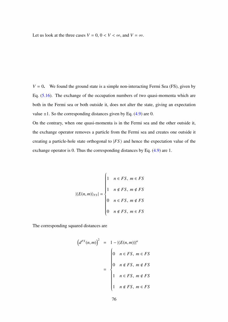
Let us look at the three cases V = 0, 0 < V < ∞, and V = ∞.
V = 0. We found the ground state is a simple non-interacting Fermi Sea (FS), given by
Eq. (5.16). The exchange of the occupation numbers of two quasi-momenta which are
both in the Fermi sea or both outside it, does not alter the state, giving an expectation
value ±1. So the corresponding distances given by Eq. (4.9) are 0.
On the contrary, when one quasi-momenta is in the Fermi sea and the other outside it,
the exchange operator removes a particle from the Fermi sea and creates one outside it
creating a particle-hole state orthogonal to |FS � and hence the expectation value of the
exchange operator is 0. Thus the corresponding distances by Eq. (4.9) are 1.
|�E(n,m)�FS | =
1 n ∈ FS , m ∈ FS
1 n � FS , m � FS
0 n ∈ FS , m � FS
0 n � FS , m ∈ FS
The corresponding squared distances are
�dFS (n,m)
�2= 1 − |�E(n,m)�|α
=
0 n ∈ FS , m ∈ FS
0 n � FS , m � FS
1 n ∈ FS , m � FS
1 n � FS , m ∈ FS
76

We relabel the momenta as n→ n, p with −N/2 ≤ n < N/2, p = ± as follows,
n− = n, − N/2 ≤ n < N/2 (5.20)
n+ = n + N − N/2 ≤ n < N/2, (5.21)
giving us, n− ∈ FS and n+ � FS .
Let I be a N × N matrix with all entries equal to 1, Inm = 1 and a 2 × 2 matrix,
τxpp� = 1 − δpp� . The distance matrix can thus be written in a compact form as,
dFS (np,mp�) = Inmτxpp� ⇒ dFS =
0 II 0
. (5.22)
We find the points are highly “clustered" because the distance matrix is the same as a
space with only two points seperated by a distance 1. One of the points represents all the
quasi-momenta in the FS and the other one represents all the quasi-momenta outside it.
This is demonstrated in the schematic figure below.
Figure 5.2: Schematic figure for the two points seperated by distance 1 as obtained fromthe distance matrix. The filled circle correspond to all the quasi-momenta modes insidethe FS and the unshaded circle represents all the quasi-momenta modes outside it.
We also find that the distance matrix reveals a sharp Fermi surface, in the sense that the
distances jump from 0 to 1 at the Fermi points.
0 < V < ∞. Numerical exact diagonalisation of the Hamiltonian, in the quasi-momentum
basis, for the 18-site system, for values of interaction strength V = 0 − 12, gives us the
quantum distance matrix.
We have chosen α = 2 in the definition of the quantum distances in Eq. (4.9).
As soon as the interaction is turned on, V = 0+, the zero distances between pairs of quasi-
77

momenta in the Fermi sea (and pairs outside it) become non-zero and are not all equal
either. Also, the distances between quasi-momenta in the Fermi sea and outside shift
slightly from 1 and are no longer all equal. The distance matrix has the following form,
d =
Δ Δe
Δe Δ
(5.23)
where Δ has all matrix elements� 1 and Δe has matrix elements slighlty less than 1. The
matrix elements of Δ increase and those of Δe decrease upon increasing V . The numerical
distance matices and their evolution with the interaction is shown in Fig. (5.3). For V ≥ 4,
� � � � � � � � � � ����������������
�
�
�
�
�
�
�
�
�
�
��
��
��
��
��
��
��
��
���
���
���
���
���
���
���
� � � � � � � � � � ����������������
�
�
�
�
�
�
�
�
�
�
��
��
��
��
��
��
��
��
���
���
���
���
���
���
���
� � � � � � � � � � ����������������
�
�
�
�
�
�
�
�
�
�
��
��
��
��
��
��
��
��
���
���
���
���
���
���
���
� � � � � � � � � � ����������������
�
�
�
�
�
�
�
�
�
�
��
��
��
��
��
��
��
��
���
���
���
���
���
���
���
� � � � � � � � � � ����������������
�
�
�
�
�
�
�
�
�
�
��
��
��
��
��
��
��
��
���
���
���
���
���
���
���
� � � � � � � � � � ����������������
�
�
�
�
�
�
�
�
�
�
��
��
��
��
��
��
��
��
���
���
���
���
���
���
���
Figure 5.3: (a)-(f) Distance matrices obtained from numerical computation for interactionstrengths V = 0.1 (a), V = 1 (b), V = 2 (c), V = 3 (d), V = 4 (e) and V = 12 (f).
the above block structure is no longer there, the matrix becomes homogenous with only
the elements d(i, i + L2 ), i = 1, · · · , L
2 differing from the rest. These are features of the
distances in the extreme CDW limit as we will soon find out.
78
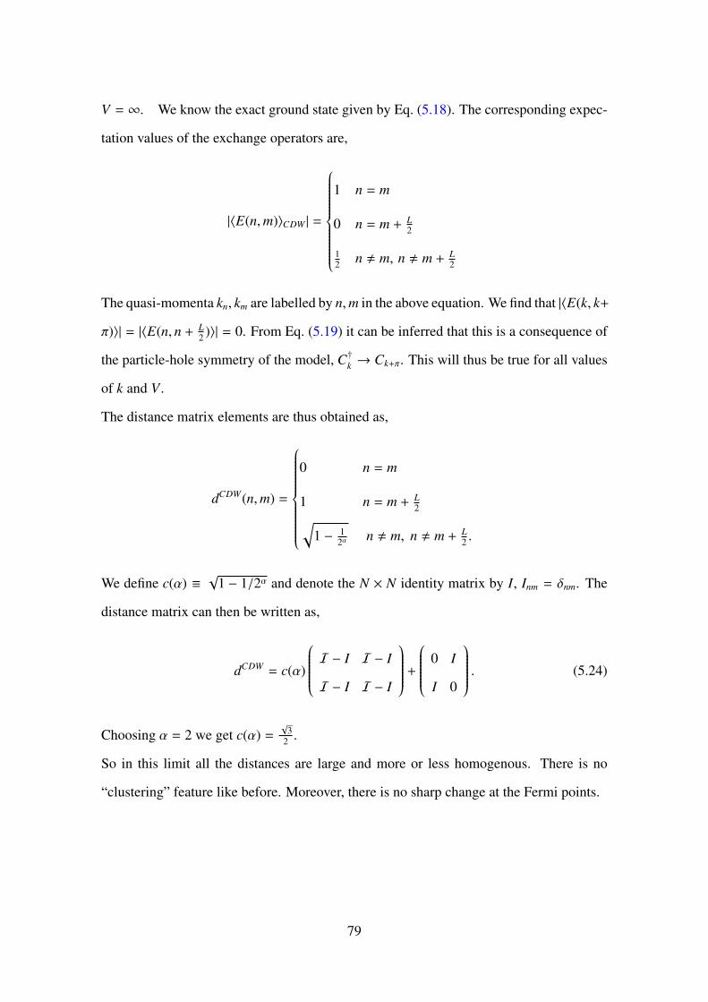
V = ∞. We know the exact ground state given by Eq. (5.18). The corresponding expec-
tation values of the exchange operators are,
|�E(n,m)�CDW | =
1 n = m
0 n = m + L2
12 n � m, n � m + L
2
The quasi-momenta kn, km are labelled by n,m in the above equation. We find that |�E(k, k+
π)�| = |�E(n, n + L2 )�| = 0. From Eq. (5.19) it can be inferred that this is a consequence of
the particle-hole symmetry of the model, C†k → Ck+π. This will thus be true for all values
of k and V .
The distance matrix elements are thus obtained as,
dCDW(n,m) =
0 n = m
1 n = m + L2
�1 − 1
2α n � m, n � m + L2 .
We define c(α) ≡ √1 − 1/2α and denote the N × N identity matrix by I, Inm = δnm. The
distance matrix can then be written as,
dCDW = c(α)
I − I I − I
I − I I − I
+
0 I
I 0
. (5.24)
Choosing α = 2 we get c(α) =√
32 .
So in this limit all the distances are large and more or less homogenous. There is no
“clustering” feature like before. Moreover, there is no sharp change at the Fermi points.
79

5.4.3 Heuristic study of the properties
We find the distances in both the interaction regime are drastically different. We have
heuristically studied the properties of the distances with particular interest in how it re-
flects the basic physics of the model.
Distances from k = −π
We first look at the the distances from a fixed point k = −π.
-3.49 -2.79 -2.09 -1.40 -0.70 0.00 0.70 1.40 2.09 2.79
k
0.0
0.2
0.4
0.6
0.8
1.0
d(−
π,k)
V=0
V=1
V=2
V=3
V=4
V=12
Figure 5.4: Distance d(−π, k) between k = −π and the other k modes in the Brillouin zone(BZ) for different values of the interaction strength V .
In Figure (5.4) we have plotted the distance d(−π, k) for different interaction strengths.
kF = ±π/2 are the Fermi points. The observations are:
1. Discontinuity at the Fermi points.
V = 0 is characterised by a jump of the distance from 0 to 1 at the Fermi points. At
large V , the discontinuity disappears. Whether the discontinuity persists for small
V we will inspect in more detail soon.
2. d(−π, 0) = 1, for all values of the interaction. This is because d(k, k+ π) = 1, for all
values of k and V , as a consequence of the particle-hole symmetry of the model.
We examine the discontinuity at the Fermi points by plotting the difference across the
Fermi points, δ = d(−π,−π2 ) − d(−π,−π2 − 2πL ), for different system sizes in Fig. (5.5). We
80

� � � � � � � � � � �� �� ��
�
���
���
���
���
���
���
δ
����
����
����
0 1 2 3 4 5 6 7 8 9 10 11 12
V
0.0
0.5
1.0
1.5
2.0
2.5
3.0
Δ
LΔ18
LΔ14
LΔ10
Figure 5.5: δ = d(−π,−π2
)−d(−π,−π2− 2π
L) and Δ: the derivative of the distance d(−π, k)
at k = −π/2, are studied as a function of interaction strength V for different system sizes,to examine the discontinuity across the Fermi points.
also look at the numerical derivative of the distance d(−π, k) at k = −π/2 which can be
defined as follows: Δ =�d(−π,−π2 + 2π
L ) − d(−π,−π2 − 2πL )
�× L
2π .
For above small systems the discontinuity seems to persist for V � 2, as we find δ is
insensitive to the system size for V � 2 and starts depending on the system size for
larger values of V . Also, the derivative Δ should tend to a constant value as a function
of L if there is no discontinuity. Which is clearly not the case in the above regime as
demonstrated in Fig. (5.5). So there is a possibility of the discontinuity persisting in the
thermodynamic limit for small values of V .
Properties of the triangles for different values of interaction
We study the properties of triangles with edges given by the distances, which are the
fundamental geometric objects. There are three types of triangles in the system when we
classify them according to the behaviour of the distances,
1. Triangles with all the vertices either inside the FS or outside it.
In the large interaction limit these are equilateral triangles and with the decrease of
interaction the edges start shrinking. Such triangles shrink to a point at V = 0, with
all the edges being zero. This is illustrated in Fig. (5.7). Such triangles are�
L2
�C3
in number and we call these triangles “particle triangles”.
81
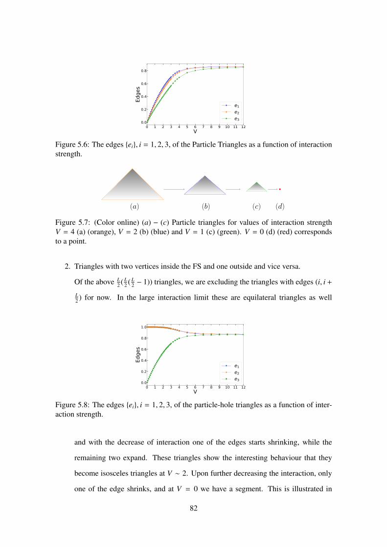
� � � � � � � � � � �� �� ��
�
���
���
���
���
���
�����
��
��
��
Figure 5.6: The edges {ei}, i = 1, 2, 3, of the Particle Triangles as a function of interactionstrength.
(a) (b) (c) (d)
Figure 5.7: (Color online) (a) − (c) Particle triangles for values of interaction strengthV = 4 (a) (orange), V = 2 (b) (blue) and V = 1 (c) (green). V = 0 (d) (red) correspondsto a point.
2. Triangles with two vertices inside the FS and one outside and vice versa.
Of the above L2 ( L
2 ( L2 − 1)) triangles, we are excluding the triangles with edges (i, i +
L2 ) for now. In the large interaction limit these are equilateral triangles as well
� � � � � � � � � � �� �� ��
�
���
���
���
���
���
���
�����
��
��
��
Figure 5.8: The edges {ei}, i = 1, 2, 3, of the particle-hole triangles as a function of inter-action strength.
and with the decrease of interaction one of the edges starts shrinking, while the
remaining two expand. These triangles show the interesting behaviour that they
become isosceles triangles at V ∼ 2. Upon further decreasing the interaction, only
one of the edge shrinks, and at V = 0 we have a segment. This is illustrated in
82

Fig. (5.9). We call such triangles “particle-hole triangles”.
(a) (b) (c) (d)
Figure 5.9: (Color online) (a)−(c) Particle-hole triangles for values of interaction strengthV = 6 (a) (purple), V = 4 (b) (orange) and V = 2 (c) (blue). V = 0 (d) (red) correspondsto a segment.
3. Triangles with the edge (i, i + L2 )
These traingles are also particle-hole triangles but only L2 × (L − 2) in number.
� � � � � � � � � � �� �� ��
�
���
���
���
���
���
���
�����
��
��
��
Figure 5.10: The edges {ei}, i = 1, 2, 3, of the particle-hole triangles with the special edge(i, i + L
2 ) as a function of interaction strength. e1 labels the constant edge (i, i + L2 ).
They are isosceles triangles in the large interaction limit. One of the edges is inde-
pendent of V , while one of the remaining two equal edges expands and the other
one contracts as V decreases. It again becomes an isosceles triangle for V � 2,
beyond which only one edge shrinks, and at V = 0 we have a segment like all other
particle-hole triangles. This is illustrated in the Fig. (5.11).
Nearest neighbour distances
We inspect the distances between neighbouring points in the BZ, (k, k + 1). The first
question which comes to mind in the context of the nearest neighbour distances is: can
83

V → 4e1 e2
e3
V → 2 V → 0
Figure 5.11: The particle-hole triangles with the edge (i, i+ L2 ) ≡ e1, for different values of
interactions. In the first and second figure the edge e3 contracts and e2 expands for V � 2.After which, for V < 2, e1 = e2 and the isosceles triangle shrinks only by shrinking ofedge e3 and becomes a segment at V = 0.
we define an infinitesimal metric as discussed in the previous chapter (Eq. (3.8))?
If the distances between two quasi-momenta decrease monotonically with the separation
between them, then we stand a chance. But this is hardly the case. As we already know,
at V = ∞, almost all the points in the BZ are equidistant. The distance detween the quasi-
momenta does not monotonically decrease with the BZ separation between them, even
for a small value of V , as shown in Fig. (5.12). We find for the distances from a reference
0.0 0.5 1.0 1.5 2.0 2.5
����
0.00
0.05
0.10
0.15
0.20
0.25
0.30
�Δ�
���,��)
Figure 5.12: Distances between kre f = −π2 and other modes kn ∈ FS , as a function of theseperation between them in the BZ, Δkre f = kn − kre f , for V = 1.
k mode −π2
(kre f ), the distance from the closest k mode is infact having the optimum value
even at a small interaction value, V = 1.
Thus the infinitesimal quantum metric g(k), defined by limΔk→0 d2(k, k + Δk) = g(k)Δk2,
84

may not be well defined in this system.
Let us have a look at the behaviour of the nearest-neighbour distance d(kn, kn+1) for dif-
ferent V , which is shown in Fig. (5.13) over half the Brillioun zone. The value of n runs
from 0 (k0 ≡ −π) to L − 1 (kL−1 ≡ π − 2πL ) over the full BZ and we consider kL ≡ −π.
The observations are,
���� ���� ���� ���� ���� ���� ���� ���� ����
��
���
���
���
���
���
���
���
�������
���
���
���
���
���
����
Figure 5.13: Nearest Neighbour Distance for different interaction strength V , over halfthe BZ.
1. V = 0, is characterised by is a delta function singularity at the Fermi point. All
the nearest neighbour distances are zero except at the Fermi point, when one quasi-
momentum is in the Fermi sea and its nearest neighbour is outside it, in which case
it is equal to 1.
2. The above singularity seems to persist for low V , and slowly smoothens when V is
increased at large V .
3. At V = ∞, all the nearest neighbour distances are equal and it can be seen that at
V = 12 this is more or less true.
85
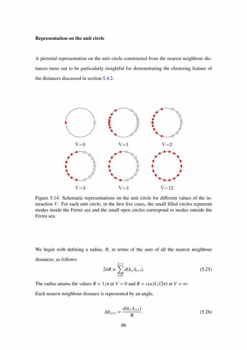
Representation on the unit circle
A pictorial representation on the unit circle constructed from the nearest neighbour dis-
tances turns out to be particularly insightful for demonstrating the clustering feature of
the distances discussed in section 5.4.2.
V=0
0
V=1 V=2
V=3 V=4 V=12
Figure 5.14: Schematic representations on the unit circle for different values of the in-teraction V . For each unit circle, in the first five cases, the small filled circles representmodes inside the Fermi sea and the small open circles correspond to modes outside theFermi sea.
We begin with defining a radius, R, in terms of the sum of all the nearest neighbour
distances, as follows:
2πR ≡L−1�
i=0
d(ki, ki+1). (5.25)
The radius attains the values R = 1/π at V = 0 and R = c(α)L/(2π) at V = ∞.
Each nearest neighbour distance is represented by an angle,
Δθi,i+1 =d(ki, ki+1)
R. (5.26)
86

Finally, an angular representation is constructed for each quasi-momentum,
θki =
i�
j=0
Δθ j−1, j (5.27)
where, Δθ−1,0 ≡ 0.
The corresponding representation on the unit circle, is shown in Fig. (5.14). At V = 0, all
the points collapse into θ = 0, π, at small V , they spread out but the points in the Fermi
sea and those outside it are well seperated. Illustrating the clustering of the points inside
(or outside) the FS together. The separation starts closing for values of V between 2 and
3, and at V ≥ 4 all points are equally spaced like the V = ∞ case and the separation is
almost invisible. Thus the features of clustering is completely washed off.
5.4.4 Conclusions
Let us summarize the results we get from the heuristic study of the properties of the
distances. We have applied exact diagonalization and looked at the quantum distances
for a finite system which consequently does not show a sharp phase transition but only
a crossover from the metallic to the insulating regime as an effect of the interaction V .
The exact diagonalization was performed using standard sparse library in Python. It was
performed to track only the first three states of the spectrum.
Our main observation is the clustering of points inside (or outside) the FS from the dis-
tances in the metallic regime which are either very small or close to 1. The distances
show signals of sharp Fermi points as well. When increasing V the distances become
homogenous and the above grouping is gone and discontinuities at the Fermi points are
lost as well.
We have illustrated this behaviour in three ways.
87

• Analysis of distances from a fixed point, k = −π, to all the others showed jumps at
the Fermi points at low V , which smoothen out slowly when increasing V , at large
V .
• The triangles formed by the distances between three quasi momenta being funda-
mental geometrical objects, have been studied them in detail. The triangles are
mostly equilateral with finite areas in the insulating regime. The area, however,
falls rapidly in the metallic regime, leaving only points and segments at V = 0.
• Inspection of nearest-neighbour distances and constructing representations of the
quasi-momenta modes on an unit circle has been quite insightful, with a nice pic-
torial demonstration of the clustering at small V and complete loss of it at large
V .
In all the three cases we observe the crossover around V = 2−4. Since the metal-insulator
transition occurs at the theoretical value V = 2[76], we conclude that the “clustering-
declustering" feature that we observe in the distance matrix is indeed characterizing the
metal-insulator crossover.
The transformation of the graph of the ground state, introduced in Sec. (5), as a function
of the interaction is rather interesting.
1
2
3
4
5
6
7
8
kinkout1
2
3
4
5
6
7
8
kinkout
w1 w2
Figure 5.15: The schematic representation of the graph of ground state of the t−V modelat V = 0 (left) and V � 0 (right). The weight of the edges for vertices given by pointsinside (or outide) the FS is denoted by w1 and the weight of the edges for one vertexinside the FS and one outside it is denoted by w2. w1 increase as a function of V , whilew2 decreases.
88

At V = 0, we have a bipartite graph with the points in the FS and outside the FS repre-
senting two group of vertices, which are disconnected amongst themselves but connected
to each other. Immediately as the interaction is switched on, V = 0+, the graph changes
character and we have a completely connected graph. But the weights of the edges given
by the distances are highly non-uniform resulting in the "clustering” of the vertices, while
at large V the graph for the insulator is a complete graph with uniform connectivity or
weights over all the edges. We will illustrate the efficiency of all the tools introduced
in previous sections by applying them to the quantum distances of the t − V model in
upcoming chapters.
89

90
Chapter 6
Euclidean Embedding of the Distances
The study of the extrinsic geometry of the correlated many-body state involves the con-
struction of vector configurations in Euclidean space, such that the vectors are separated
from each other by distances prescribed by the matrix of quantum distances D (Eq. ( 5.1
)). This brings us to the fascinating subject of distance geometry developed by mathemati-
cians like Cayley[55], Menger[56], Bluementhal[57], Schoenberg[54] and Godel[77],
which focuses on the study of geometry in terms of distances.
In the context of our work, it is interesting to understand the properties of the embedding:
what is the dimension of the Euclidean space and what kind of vector configurations arise
in our objective of realizing quantum distances?
A lot of researchers in other branches of science have asked similar questions. Seeking
the vector configuration of points from a set of noisy or incomplete distances is a topic
of active research[53]. Applications include finding 3D configurations of molecules from
NMR data with particular success in finding the structure of proteins[78]. In the Wireless
Sensor Network Localization problem (WSNL), the relative distance of sensor networks
estimated by recording the power loss during a two-way exchange are used to find the
positions of each sensor[79]. Multidimensional scaling, i.e., the problem of finding a set
of vectors in smaller dimensions starting from a higher dimensional space, is popularly
91

used in data visualization[80].
Contrary to some of the popular applications listed above, the problem we have at hand
is simpler, because we have the accurate and complete distance matrix D. If the distance
matrix D can be an EDM, then it can be easily found by constructing the Gram matrix
as per Eq. (6.10) and inspecting the eigenvalues, as a direct consequence of Schoenberg’s
theorem (1) discussed in Sec. (5.2). The dimension of the Euclidean space is given by the
rank of the Gram matrix and the configuration of the point set in above Euclidean space
is obtained by the spectral decomposition of the Gram matrix (Eq. (6.11)).
6.1 Embedding of mean field states
Before entering into the machinery of distance geometry, let us have a look at the Eu-
clidean embedding of the distance matrices obtained from the mean-field states. For the
mean field states our definition of the quantum distances reduces to the standard one in
terms of overlap of the single particle wavefunctions, given by Eq. (3.8).
Let us first look at the choice α = 1, in our definition of distances in Eq. (4.9), which
gives the Hilbert-Schmidt distances for the mean field states. For a N-dimensional Hilbert
space,HN , the matrix of Hilbert-Schmidt distances between two states |Ψn�, |Ψm� ∈ HN ,
is
(D(n,m))2 = 1 − tr (ρn ρm) (6.1)
where ρn ≡ |Ψn��Ψn|. Let us consider the N2 generators of U(N): the identity operator I
and the generators of SU(N): Tα, α = 1, . . . ,N2 − 1. The above generators satisfy the
conditions
(Tα)† = Tα, tr (Tα) = 0,12
tr�TαT β
�= δαβ. (6.2)
We know that any linear Hermitian operator in HN can be expressed as a linear combi-
nation of the generators of U(N) in the fundamental representation. Then, ρn can then be
92

expressed as,
ρn =1N+ �an · �T , aαn =
12
tr (Tαρn) . (6.3)
The vector �a in above equation is a real N2 − 1 dimensional vector, i.e �an ∈ R(N2−1), since
we know Tα and ρn are Hermitian matrices.
From the basic properties ρ2n = ρn and tr ρn = 1,
�an · �an =12
�1 − 1
N
�. (6.4)
Equation (6.1) can be rewritten as
(D(n,m))2 = 1 − 1N− 2�an · �am (6.5)
= |�an − �am|2. (6.6)
Thus the Hilbert-Schmidt distance matrix of mean field states of systems with transla-
tional symmetry can be isometrically embedded in a finite dimensional Euclidean space,
R(n2b−1), for a nb orbital model, irrespective of the system size.
Let us consider an arbitrary α in Eq. (4.9) in the definition of the distances. The distance
between neighbouring points k and k + dk, in the limit dk→ 0 is
(Dα(k, k + dk))2 = 1 − (trρ(k)ρ(k + dk))α
= 1 −�1 − |�a(k + dk) − �a(k)|2
�α.
Assuming �a(k) to be a smooth function of k, because the wave functions |Ψ(k)� are them-
selves so, it holds that
(Dα(k, k + dk))2 = α∂�a(k)∂kµ
· ∂�a(k)∂kν
dkµ dkν (6.7)
≡ gµνα (k) dkµ dkν. (6.8)
93

This implies the distances between neigbouring points in the spectral parameters are just
scaled by the factor α, in the thermodynamic limit,
gµνα (k) = αgµν1 (k). (6.9)
So we can conclude for α � 1, although the Euclidean embedding in (n2b − 1) dimensional
space obtained for α = 1 will not be isometric, the shape of the embedded surface is
independent of α up to a scaling factor.
6.2 Isometric Euclidean embedding
1. Construct the Gram matrix,
G = −12
(I − 1Ld eeT )D2(I − 1
Ld eeT ). (6.10)
I is the Ld × Ld identity matrix. e is a Ld-dimensional column vector with allentries equal to 1.
2. Check if it is positive semi definite (PSD) with only positive eigenvalues.
3. The rank of G, if it is PSD, corresponds to the dimension of the Euclidean spacein which the distances can be embedded.
4. The configuration of the Ld embedded vectors {xi} is obtained by diagonaliza-tion of the above real symmetric matrix G,
G(i, j) = xi.x j = (U√Λ)(√ΛUT ). (6.11)
Figure 6.1: Algorithm for isometric embedding of quantum distances.
The algorithm for isometric embedding of the matrix of quantum distances D is rather
simple and a direct consequence of the Schoenberg’s theorem (1), proposed by Isaac
Schoenberg in 1935[54]. It has been detailed in Fig. (6.1). The volume of N simplices as
obtained from the Cayley-Menger determinant Δ, which is constructed from the distance
94

matrix as follows[55, 56],
Δ = Det(CD), (6.12)
CD =
0 1 1 .. 1
1 0 D1,2 .. D1,N
...
1 DN,1 DN,2 .. 0
(6.13)
V2N =
(−1)N−1
2N(N!)2Δ, (6.14)
should reflect the same result.
If the dimension of Euclidean embedding is obtained to be r, which is the rank of the G
matrix, we should find the volume of all N simplices for N ≤ r+ 1 should be nonzero and
higher order simplices should be zero, as per Bluementhal’s theorem (2)[57].
6.2.1 Isometric embedding of the distance matrix of t − V model
We apply the above scheme to the L×L matrix of quantum distances of the half filled one-
dimensional t − V model, for different values of interaction V , discussed in Sec. (5.4.2).
We look at the three cases, V = 0, V = ∞, and 0 < V < ∞ in this section.
V = 0. At V = 0, the ground state is a mean field state (the Fermi sea) with all the single
particle states with energies less than zero occupied and those with energies greater than
zero unoccupied. The quasi-momenta corresponding to the occupied single particle states
we label as kin and those for the unoccupied single particle states by kout.
The distance matrix, DFS obtained in Eq. (5.22) has the following form,
DFS (kin, kin) = 0 = DFS (kout, kout) (6.15)
DFS (kin, kout) = 1 = DFS (kout, kin). (6.16)
95

The Gram matrix has only one non-zero eigenvalue, λ = L4 and the distance matrix can be
embedded in a one dimensional Euclidean space,
x(kin) = −0.5, x(kout) = 0.5. (6.17)
V = ∞. The matrix of the squared distances, D2CDW , using Eq. (5.24) can be written as:
D2CDW =
34
I − I I − I
I − I I − I
+
0 I
I 0
. (6.18)
I is a N × N matrix (N = L2 ) with all entries equal to 1, I is the identity matrix and e is
defined below equation(6.10) and eeT = I. The Gram matrix defined in equation(6.10)
is,
GCDW = −12
AD2CDW A (6.19)
A ≡
I 0
0 I
−1L
I II I
. (6.20)
We find that,�A,D2
CDW
�= 0 ⇒ [A,GCDW] = 0 (6.21)
Thus, A and GCDW have the same eigenvectors.
Let us define a complete, orthonormal set of L2 dimensional column vectors aµ, µ = 1... L2 ,
where a1 =
�2L (1, 1, . . . , 1)T . A complete set of L dimensional orthonormal vectors is
96

then defined as follows,
bi =
1√2
ai
ai
i = 1, . . . , L
2
1√2
ai−L/2
−ai−L/2
i = L
2 + 1, . . . , L.
. (6.22)
Therefore,
GCDWb1 = 0 (6.23)
GCDWbi =
14bi i = 2, . . . , L
2
12bi i = L
2 + 1, . . . , L. (6.24)
Thus,
(GCDW)i j =
L/2�
k=2
14
bki b
kj +
L�
k=L/2+1
12
bki b
kj. (6.25)
Thus the explicit solution for the embedding is found to be the L, (L − 1)-dimensional
vectors, xi, i = 1, . . . , L, with components, (xi)n , n = 1, . . . , L − 1, given by
(xi)n =12
bn+1i , n = 1, . . . ,
L2− 1 (6.26)
=1√2
bn+1i , n =
L2, . . . , (L − 1). (6.27)
The distance matrix at V = ∞, can be isometrically embedded in a Euclidean space with
dimension equal to L − 1.
0 < V < ∞. We have obtained the numerical distance matrix applying exact diagonal-
ization for system sizes L ≤ 18 and interaction values, V = 0 − 12. Applying the above
scheme we find, as soon as the interaction is turned on, the exact rank of the Gram matrix
97

becomes thermodynamically large, i.e L − 1 and remains so till V = 12. The result in
the CDW limit suggests for the insulating phase the dimension of Euclidean embedding
is indeed scaling as system size. But for smaller values of V this is counterintuitive.
0 1 2 3 4 5 6 7 8
V
0.000
0.005
0.010
0.015
0.020
0.025
0.030
0.035
0.040
Δ
Figure 6.2: Volume of the L simplex as a function of the interaction, for 18 sites.
For small values of V , the state is not very different from the mean field state although
we know that as soon as interactions are turned on, the system goes from a Fermi liquid
to a Luttinger liquid. The state, though qualitatively different, still remains metallic till
V/t = 2. Besides, we also find that the spectrum of the Gram matrix does not drastically
change, the largest eigenvalue shifts very little from the previous value L4 (at V = 0) and
most of the smaller eigenvalues are insignificant. We look at the volume of the L simplex,
in Fig. (6.2) and find that it remains very small in the metallic regime, although the exact
rank is L − 1, suggesting the effective embedding still has a lower dimensionality.
It is thus natural to ask whether the distance matrix can still be approximately embedded
in a finite-dimensional Euclidean space in some precise sense, in the metallic regime.
In a more general context, we would like to visualize the embedding in lower dimensional
spaces and associate “shapes” and surfaces to the distances obtained from the correlated
state, for a characterisation of the extrinsic geometry. Thus even if the embedding dimen-
sion scales with the system size, if an approximate embedding scheme exists we can do
98

so.
There are several methods for approximate embedding of a distance matrix in a Euclidean
space [58, 59, 60, 61, 62], two of which we investigate in next section.
6.3 Approximate Euclidean Embedding
We seek approximate embedding of the quantum distances into a smaller dimensional
(1 − 3) Euclidean space where visualisation of the vectors is possible. The cost that we
pay is that the embedding is no longer isometric. But there are well defined concepts of
quantitative estimation of the accuracy of such approximations. We consider two such
approaches, the first being the truncation of the spectrum of the Gram matrix with an
estimate of error[61, 62] and the second being the method of average distortion[59, 60].
6.3.1 Truncation of Gram matrix spectrum with error estimate
The effective rank of the numerical Gram matrix is very difficult to determine, because
the effective zeros also manifest in the spectrum as small numerical values.
So the precise question we are asking is, how many eigenvalues from the Gram matrix
spectrum we should retain or how many eigenvalues could we safely discard?
Similar questions are asked by people in data mining[61, 62] where for dimensionality
reduction of huge dataset, they look into Prinicipal Component Analysis and discard the
smaller eigenvalues of the covariance matrix with an error estimate or for data mining
applications where people use truncated Singular Value Decomposition. We extend the
most common method used in above applications, retain the first few largest singular
values or eigenvalues and estimate the corresponding squared error from the ratio of the
sum of the eigenvalues to the total sum of eigenvalues. Then we keep as many eigenvalues
such that this error remains within a threshold value of 10% − 20%.
99

The diagonalisation of the Gram matrix, which is a real symmetric Ld × Ld matrix, gives
G = UΛUT (6.28)
where U is an orthogonal matrix and Λ a diagonal matrix. We choose a basis obtained by
arranging the eigenvalues in the order of their magnitude, Λ11 ≥ Λ22 ≥ · · · ≥ ΛLdLd .
Retaining only the highest q diagonal entries we obtain an approximate Gram matrix in
the diagonal basis, Λ, where Λii = Λii, i ≤ q, Λii = 0, i > q. The approximate Gram
matrix G with rank q will be,
G ≡ UΛUT . (6.29)
We define the corresponding truncation error as,
E(q) = 1 −� �q
i=1Λii�Ld
k=1Λkk
. (6.30)
Let us now demonstrate the method with the t − V model,
� � � � � � � � � � �� �� ��
�
���
���
���
���
���
���
���
���
���
� ���
���
���
Figure 6.3: Truncation error for keeping first few (1-3) eigenvalues of G. The error forapproximate embedding is less than 12% in case of embedding in one dimension E(q = 1)up to V ≈ 1.5 and for embedding in three dimension E(q = 3) up to V ≈ 2.
Fig. (6.3) clearly shows that the truncation error for retaining first few largest eigenvalues
(1 ≤ q ≤ 3) is quite small, less than 12%, for V < 2. So an approximate embedding into
smaller dimensions is indeed possible in the metallic phase. However, for V > 2 such
100

an approximation will be highly inaccurate as indicated by the error estimate. So in the
insulating phase the dimension of even the approximate embedding is definitely greater
than 3.
6.3.2 Average distortion
The next method of approximate embedding we follow, is that of average distortion.
The concept of distortion originated in theoretical computer science in the context of
metric embedding, or defining a map from a metric space (K, d) to another simpler host
metric space (H, ∂), f : K → H, where the faithfulness of the embedding is measured
by the distortion[58]. The distortion � is an estimate of how close the distances between
points in (H, ∂) resemble that in (K, d), and is defined as[59],
� = maxx,y∈Kd(x, y)∂(x, y)
. (6.31)
Another global estimate of accuracy is the average distortion �avg, defined as follows[59,
60],
�avg =
�x,y∈K d(x, y)
�x,y∈K ∂(x, y)
. (6.32)
Let us begin with the set of Ld vectors in r dimensions (rank of G), {xi} (i = 1, . . . , Ld),
xi ∈ R(r), obtained from isometric Euclidean embedding by diagonalising the Gram ma-
trix.
We choose q of the basis vectors and look at each of the (Ld − 1)Cq, q-dimensional sub-
spaces. Let D(i, j) be the corresponding new distances in the q dimensional Euclidean
space. The average distortion for each case is given by,
�avg ≡�
i, j D(i, j)�
i, j D(i, j). (6.33)
We compute the average distortion in each case and pick the subspace that minimizes it.
101

We label the above minimum value of average distortion as �min. Lower values of average
distortion could perhaps be obtained by rotating the basis set. In our application to the
distance matrices of the t − V model we have however considered only the choice of q of
the basis vectors.
� � � � � � � � �
�
����
����
����
����
����
����
����
����
����
����εmin
q��
q��
q��
Figure 6.4: Average distortion for approximate embedding of D in lower dimensions as afunction of interaction strength.
The average distortion as a function of interaction strength for q = 1, 2, 3 is plotted in
Fig. (6.4). We find embedding with values of average distortion very close to the ideal
value one is possible only for small values of interaction, V � 2. The maximum average
distortion allowed corresponding to the upper bound of error 0.12 in region V � 2 is
found to be 1.27. In the insulating phase approximate embedding in lower dimensions is
not possible as indicated by the high values of average distortion.
102

Chapter 7
Wasserstein Distances
The geometry of the many-body state can also be studied by constructing probability dis-
tributions from the quantum distances. The central technique of our choice is the powerful
theory of optimal transport[63, 64]: it is used to construct geometric observables from the
distance distributions. In general, optimal transport theory gives us the necessary tools to
perform a thorough analysis of the geometry of the distance distributions. In particular,
it provides us with a new metric called the Wasserstein distance, which is essentially a
measure of distance between probability distributions.
In this chapter we focus on the Wasserstein distances which are found to be particularly
successful in capturing the phases of the many-body state. Using these distances, we
obtain a very sharp characterisation of the phases of the ground state. Moreover they are
interesting in our context because they are obtained by averaging over the full spectral
parameter space.
103
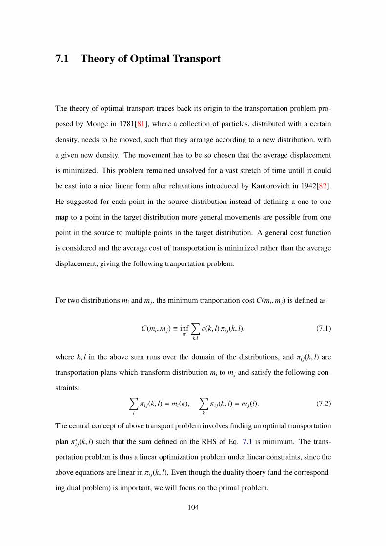
7.1 Theory of Optimal Transport
The theory of optimal transport traces back its origin to the transportation problem pro-
posed by Monge in 1781[81], where a collection of particles, distributed with a certain
density, needs to be moved, such that they arrange according to a new distribution, with
a given new density. The movement has to be so chosen that the average displacement
is minimized. This problem remained unsolved for a vast stretch of time untill it could
be cast into a nice linear form after relaxations introduced by Kantorovich in 1942[82].
He suggested for each point in the source distribution instead of defining a one-to-one
map to a point in the target distribution more general movements are possible from one
point in the source to multiple points in the target distribution. A general cost function
is considered and the average cost of transportation is minimized rather than the average
displacement, giving the following tranportation problem.
For two distributions mi and mj, the minimum tranportation cost C(mi,mj) is defined as
C(mi,mj) ≡ infπ
�
k,l
c(k, l) πi j(k, l), (7.1)
where k, l in the above sum runs over the domain of the distributions, and πi j(k, l) are
transportation plans which transform distribution mi to mj and satisfy the following con-
straints:�
l
πi j(k, l) = mi(k),�
k
πi j(k, l) = mj(l). (7.2)
The central concept of above transport problem involves finding an optimal transportation
plan π∗i j(k, l) such that the sum defined on the RHS of Eq. 7.1 is minimum. The trans-
portation problem is thus a linear optimization problem under linear constraints, since the
above equations are linear in πi j(k, l). Even though the duality thoery (and the correspond-
ing dual problem) is important, we will focus on the primal problem.
104

7.1.1 Basic definitions
1. We construct the normalised distribution of distances mi, from the distance ma-trix D as follows,
mi( j) =D(i, j)�k D(i, k)
(7.3)
2. The system of equations (7.9-7.10) is casted as a linear programming problem:
W (p)(i, j) = infΠ≥0
�DTΠ
�(7.4)
ATΠ = η. (7.5)
Where D is a L2d component column matrix defined as follows:
D = ((d(1, 1))p, ....(d(1, Ld))p, (d(2, 1))p, . . . (d(Ld, 1))p, ....(d(Ld, Ld))p)T ,(7.6)
Π is a L2d component column matrix and η is a 2Ld component column matrixconstructed from the two distributions mi and mj,
η = (mi(1), ....mi(Ld),mj(1), ....mj(Ld))T . (7.7)
AT =
1 1 ... 1 0 0 ... 0 ... 0 0 ... 00 0 ... 0 1 1 ... 1 ... 0 0 ... 0...... ..
......... ..
... ......... ..
...0 0 ... 0 0 0 ... 0 ... 1 1 ... 11 0 ... 0 1 0 ... 0 ... 1 0 ... 00 1 ... 0 0 1 ... 0 ... 0 1 ... 0...... ..
......... ..
... ......... ..
...0 0 ... 1 0 0 ... 1 ... 0 0 ... 1
(7.8)
AT is a (2Ld × L2d) matrix.
Figure 7.1: Algorithm for computation of the Wasserstein distance starting from the ma-trix of quantum distances D
Let us return back to the probability distributions and review the definition of the Wasser-
stein distances introduced in Sec. (5.3.2).
The pth Wasserstein distance between two probability distribution functions (PDFs) mi
and mj, Wp(mi,mj), is defined as follows:
105

W (p)p (mi,mj) ≡ inf
π
�
k,l
(d(k, l))pπi j(k, l), (7.9)
where k, l in the above sum runs over the domain of the PDFS, p ∈ [1,∞) and πi j(k, l) is
joint probability distribution whose marginals are mi and mj,
�
l
πi j(k, l) = mi(k),�
k
πi j(k, l) = mj(l). (7.10)
The pth root of the above optimised function W (p)p (mi,mj) satisfies all the axioms of a dis-
tance function only when d(k, l) is a valid distance function and satisfies all the properties
of a metric.
The underlying theory of optimal transport and the Wasserstein distances are widely used
in solution of partial differential equations, fluid mechanics, proability theory, statistics
and discrete differential geometry. The fields of application include image retrieval[83],
computer vision[84], economics and finance[85], to name some.
For our problem in quantum geometry, mi and mj are the distance distributions defined in
Eq. (5.8) of Sec. (5.3.1) in Chapter 5, at any two points ki and k j in the space of spectral
parameter.
While d(k, l) can be any valid distance defined between the points in the spectral parameter
space, we have studied the quantum distances and the Euclidean distances (detailed later).
Choosing p = 2 in Eq. 7.9, we have looked at squared 2-Wasserstein distances, W (2)(mi,mj),
between any two PDFs mi and mj, defined as follows,
W (2)(mi,mj) ≡ infπ
�
k,l
(d(k, l))2πi j(k, l). (7.11)
Here πi j satisfies the constraints given by Eq. (7.10).
The corresponding squared Wasserstein distance between the distance distributions, given
by the above sum in Eq. (7.11) then gives the weighted average of all the squared distances
between any two points in the spectral parameter space, with the corresponding weights
106

specified by the optimal joint probability distribution π∗i j. We discuss them in more detail
alongwith the results obtained in the t − V model in Sections 7.2 and 7.3.
The Ollivier-Ricci curvature which is a generalization of the Ricci curvature in a discrete
setting is closely related to the 1-Wasserstein distance, W(mi,mj), corresponding to the
choice p = 1 in Eq. (7.9) and the distance function d(k, l) being the quantum distances,
W(mi,mj) ≡ infπ
�
kl
D(k, l)πi j(k, l). (7.12)
We will discuss this in great detail in Chapter 9. We look at the Euclidean embedding of
the Wasserstein distance W(mi,mj) in Section 7.4.
7.2 Wasserstein distances defined from the quantum dis-
tances
We define squared Wasserstein distances between two distance distributions mi and mj
by choosing the distance function in the spectral parameter space, d(i, j), in the RHS of
Eq. (7.11) to be the quantum distances.
W (2)(mi,mj) ≡ infπ
Ld�
k,l=1
(D(k, l))2πi j(k, l). (7.13)
Where πi j satisfies the usual constraints given by Eq. 7.10.
7.2.1 Physical Interpretation
In our study of quantum geometry of many-fermion states, the kinematics of the state is
being studied and hence there is no time evolution and no concept of “transport" exists.
So physically what does the Wasserstein distance mean for us?
107

Since our definition is derived completely from the quantum distances in Eq. (7.13), we
can attempt to answer the above question by looking into physical interpretation of the
Wasserstein distances in terms of quantities in the Hilbert space.
The matrix of squared distances defined in equation (4.9) can be written as,
(D(i, j))2 ≡ 1 − Tr ( ρ(i, j)ρ0 ) (7.14)
ρ0 ≡ |ψ��ψ| (7.15)
ρ(i, j) ≡ E(i, j)|ψ��ψ|E(i, j) (7.16)
We call the subspace spanned by the states E(i, j)|ψ� ≡ |i, j� as quantum distance Hilbert
space, QDH, since the distance matrix is defined in this subspace. It includes the many-
body state under inspection trivially, because E(i, i)|ψ� ≡ |ψ�.
Let π∗i j(k, l) denote the optimal joint probability distribution function, for a set of distri-
butions mi and mj obtained by minimising the sum defined on the RHS of Eq. 7.13. We
define mixed states, ρ�(i, j) in QDH by,
ρ�(i, j) ≡�
k,l
π∗i j(k, l)|k, l��k, l|. (7.17)
Eq. 7.13 can then be rewritten as,
W (2)(mi,mj) = 1 − Tr(ρ0ρ�). (7.18)
The squared Wasserstein distance, W (2)(mi,mj), can thus be expressed in terms of quanti-
ties in the QDH.
108

7.2.2 Results for the t-V model
The Wasserstein distance defined above, compares a set of distance distributions quanti-
tatively and gives the distance between any two distributions. We will illustrate the effi-
ciency of the Wasserstein distances in characterising the phases of the many-body state by
application to the one-dimensional t − V model. In this section we discuss the results we
get from analytic calculations at the extreme interaction limit and the linear programming
solutions for the intermediate values of V . But first, let us inspect the distance distribu-
tions for the t − V model, because they are the fundamental object of study in optimal
transport theory.
The distance distribution functions
The quantum distances between two points in the BZ in one band models calculated using
Eq. (4.33), can be qualitatively thought of as a measure of the difference in the occupan-
cies at these two quasi-momenta. Maintaining consistency with above idea, our numerical
results for the one dimensional t−V model (Sec. (5.4.2)) showed that deep in the metallic
regime (V � 1), the distances classify the quasi momenta inside the Fermi sea, which we
labelled kin, and those outside it, which we labelled kout into two different categories. The
distances between any two points both inside or outside the Fermi sea are very small (∼ 0)
and those between two points, where one lies inside the Fermi sea and the other outside
it, are very large (1).
On the other hand, deep in the insulating regime (V � 1), the distances are rather ho-
mogenous and there is not much distinction between quasi-momenta in the Fermi sea and
those outside it.
The above behaviour can be well demonstrated by the probability distributions {mi( j)},defined at each point in the BZ, i = 1, . . . , L, constructed from normalised distribution
of distances of all the points in the BZ from the above point ki, defined as per Eq. (7.3).
109

����
�����
Figure 7.2: Schematic figure depicting the distribution functions, mi( j) (i, j = 1, ..., L),defined at each point in the BZ for the two regimes of interaction, for 18 sites. The firstfive distributions depicted with filled circles represent distribution functions at alternatepoints for quasi-momenta modes inside the Fermi sea, mkin . While the remaining fivedepicted using unshaded circles represent distributions for quasi momenta modes outsideit, mkout . In deep metallic regime, at V = 0.1, the first five distributions are completelyopposite of the next five. However, for deep insulating regime, at V = 12, mi are almostidentical for all ki ∈ kin, kout, differing only at points i, i + L
2 .
The distance distributions {mi( j)} are completely opposite of each other for points inside
the Fermi sea and points outside it and exactly identical for all points inside (or outside)
the Fermi sea in the deep metallic regime. In sharp contrast to this, in the deep insulating
regime, the distribution for every point in the BZ are almost identical, differing only at
the points (i, i + L2 ). This is illustrated in the Fig. (7.2).
Squared Wasserstein distances
0.00 0.01 0.02 0.03 0.04 0.05 0.06 0.07 0.08 0.09 0.10
1/�
0.00
0.02
0.04
0.06
0.08
�(2)
∞
Figure 7.3: W (2)∞ as a function of the inverse system size L−1 for system sizes L = 10− 28.
It is found to be linear in L−1 and thus vanishes in the thermodynamic limit.
Starting from the analytical quantum distances (Eqs. (5.22,5.24)), at extreme values of the
110

interaction, which we label as D0/∞(i, j), the corresponding squared Wasserstein distances
which we denote as W (2)0/∞(mi,mj), can be shown to be (calculations in Appendix),
W (2)0 (mi,mj) = (D0(i, j))2
W (2)∞ (mi,mj) =
1L (D∞(i, j))2, (7.19)
where L =√
32 (L − 2) + 1.
Thus, calculations indicate the Wasserstein distances become zero in insulating phase in
the thermodynamic limit. While, W (2)(mkin ,mkout), will most probably be large and non-
zero in the metallic limit.
We further compute the Wasserstein distances numerically at V = ∞, choosing the
distance distributions as obtained from the analytical distance matrices (Eq. 5.24) as
marginals, for system sizes L = 10 − 28. We have studied the corresponding uniform
squared distances, W (2)∞ , as a function of the inverse of system size in Fig. (7.3) and found
it is linear in L−1, and thus consistent with Eq. 7.19.
The numerical W (2) matrices obtained for interaction values 0 < V ≤ 12 are shown in Fig.
(7.4).
In deep metallic regime, as one would expect, the matrices have a block structure. Wasser-
stein distances W (2)(mkin ,mkin) (or W (2)(mkout ,mkout)) are very small (∼ 0), where both the
marginals are ditributions defined at points inside (or outside) the FS, reflecting the fact
that the distance distributions are almost identical.
While for the Wasserstein distances, W (2)(mkin ,mkout), where one of the marginal corre-
sponds to the distribution defined at points inside the FS, kin and the other one corresponds
to the distribution defined at points outside the FS, kout, are very large (∼ 1), as a reflection
of the fact that the distributions are completely opposite to each other.
On the contrary, in deep insulating regime the distance distributions are homogenous and
almost identical so the Wasserstein distances are uniform and almost zero.
111

Figure 7.4: (a)-(f)Squared Wasserstein Distance matrices W (2)(mi,mj) for L = 18, ob-tained from numerical computation for interaction strengths V = 0.1 (a), V = 1 (b), V = 2(c), V = 3 (d), V = 4 (e) and V = 12 (f). For i < 9, the quasi momenta modes lie insidethe Fermi sea, ki ∈ kin and for i ≥ 9, the quasi-momenta modes lie outside it, ki ∈ kout.The deep metallic regime is characterised by ∼ 0,∼ 1 distance values between kin − kin
(kout − kout) and kin − kout blocks respectively. The deep insulating regime is characterisedby uniform extremely small values very close to zero.
The converged optimal joint probability distribution, π∗, obtained from linear program-
ming solutions in the metallic and insulating regime for the two different types of trans-
port, where one of the marginal is mkin and the other one is mkout , and where both the
marginals are mkin , are shown in Fig. (7.5).
The behaviour of the distances W (2)(mkin ,mkin) as a function of the interaction strength V
for different system sizes is shown in Fig. (7.6). We can expect W (2)(mkin ,mkin) to indi-
cate the critical interaction strength for the Luttinger liquid to CDW transition, by the
occurence of a peak in the thermodynamic limit.
The behaviour of the distances W (2)(mkin ,mkout) as a function of the interaction strength V ,
for different system sizes is shown in Fig. (7.7).
From the above figures we can conjecture in the thermodynamic limit, for V � 4, in the
112

���
�������
�
�������
� � � � � � � � � � ����������������
�
�
�
�
�
�
�
�
�
�
��
��
��
��
��
��
��
�� ����
����
����
����
����
����
���
������
�
�������
� � � � � � � � � � ����������������
�
�
�
�
�
�
�
�
�
�
��
��
��
��
��
��
��
�� ����
����
����
����
����
����
���
�������
�
�������
� � � � � � � � � � ����������������
�
�
�
�
�
�
�
�
�
�
��
��
��
��
��
��
��
�� ����
����
����
����
����
����
���
������
�
�������
� � � � � � � � � � ����������������
�
�
�
�
�
�
�
�
�
�
��
��
��
��
��
��
��
�� ����
����
����
����
����
����
Figure 7.5: (a)-(d) The converged optimal joint probability distribution π∗i j, for L = 18,obtained from numerical linear programming for interaction strengths V = 1, i ∈ kin, j ∈kout (a), V = 1, i ∈ kin, j ∈ kin (b), V = 8, i ∈ kin, j ∈ kout (c) and V = 8, i ∈ kin, j ∈ kin
(d). The marginals are plotted along the corresponding axis. In the insulating regime thematrix is rather sparse differing only at i, j, i + L
2 and j + L2 in Figs. (c,d), in the metallic
regime, π∗kin,kinis relatively sparse in Fig. (b), but π∗kin,kout
in Fig. (a) is quite different withmatrix elements having significantly larger values.
� � � � � � � � � � �� �� ��
�
����
����
����
����
����
����
���
� ��
�����
����
����
����
����
Figure 7.6: Squared Wasserstein distances between distributions defined at quasi-momenta modes inside the Fermi sea, W (2)(mkin ,mkin), as a function of the interactionstrength V , for system sizes L = 10, 14, 18.
insulating phase the squared Wasserstein distances W (2) becomes zero, however, they are
non-zero in the metallic phase.
The Wasserstein distances thus gives a vivid geometric description of the ground state in
113

� � � � � � � � � � �� ��
�
���
���
���
���
���
���
� ��
�����
�����
����
����
����
Figure 7.7: Squared Wasserstein distances between distributions defined at quasi-momenta modes inside the Fermi sea and those outside it, W (2)(mkin ,mkout), as a functionof the interaction strength V for system sizes L = 10, 14, 18.
both the phases. It characterises the metallic phase by classifying the points inside the
Fermi sea and those outside it in two different groups. Most importantly, in the thermo-
dynamic limit, the Wasserstein distances become zero in the insulating phase while they
are non-zero in the metallic phase, providing a sharp characterisation of the phases of the
system.
7.3 Wasserstein distances defined from the Euclidean dis-
tances
We define squared Wasserstein distances between two distance distributions mi and mj
by choosing the distance function in the spectral parameter space, d(i, j), in the RHS of
Eq. (7.11) to be the Euclidean distances.
W (2)E (mi,mj) ≡ inf
π
L�
k,l=1
(k − l)2πi j(k, l), (7.20)
where πi j satisfies the constraints given by Eq. 7.10.We cannot connect W (2)E to quantities
in the Hilbert space like before, since the distance function is no longer derived from
states in the Hilbert space. It can neither be connected to the intrinsic curvature as before.
114

But it is an important geometric observable for the many-body state, because it probes
the geometry of the distance distribution functions, which are derived from the quantum
distances. We demonstrate this by application to the t − V model.
Figure 7.8: (a)-(d)Squared Wasserstein Distance matrices W (2)E (mi,mj) for L = 18, ob-
tained from numerical computation for interaction strengths V = 0.1 (a), V = 2 (b), V = 4(c), and V = 12 (d). For i < 9, the quasi momenta modes lie inside the Fermi sea,ki ∈ kin and for i ≥ 9, the quasi-momenta modes lie outside it, ki ∈ kout. The deep metallicregime is characterised by ∼ 0,∼ 20 distance values between kin − kin (kout − kout) andkin − kout blocks respectively. The deep insulating regime is characterised by uniform andextremely small values.
The numerical W (2)E matrices were obtained for interaction values 0 < V ≤ 12, choosing
the marginals to be the distribution functions constructed from the distance matrices ob-
tained by performing exact diagonalization. They are shown in Fig. (7.8). The squared
Wasserstein distances, W (2)E (mkin ,mkin) (or W (2)
E (mkout ,mkout)), for both the marginals being
distributions corresponding to points inside or outside the FS, are very small (∼ 0), while
W (2)E (mkin ,mkout) for the marginals being a distribution defined at a quasi-momenta mode
inside the FS and another distribution defined at quasi-momenta mode outside it, are very
large (∼ 20). Whereas, in deep insulating regime the Wasserstein distances are uniform
and very small.
115

Thus, we find the overall behaviour as one would expect, is similar to that found for the
squared Wasserstein distances defined from the quantum distances.
The behaviour of both types of distances as a function of the interaction strength V , how-
ever, seems to be more revealing.
The distances W (2)E (mkin ,mkin), as a function of the interaction strength V , for different
� � � � � � � � � � �� �� ��
�
����
����
����
����
����
����
����
���
��
�������
����
����
����
����
Figure 7.9: Squared Wasserstein distances between distributions defined at quasi-momenta modes inside the Fermi sea, W (2)
E (mkin ,mkin), as a function of the interactionstrength V , for system sizes L = 10, 14, 18. The above distances show a prominent peakat V = 2.4, for L > 10.
system sizes is plotted in Fig. (7.9). These distances indicate the transition by a peak, at
V = 2.4, which we expect to be more sharpened in the thermodynamic limit.
The distances W (2)E (mkin ,mkout) as a function of the interaction strength V , for different
system sizes is plotted in Fig. (7.10).
We find, in the regime V � 2.4, that W (2)E (mkin ,mkout) scales proportionally with the system
size, after which it is insensitive to system size and constant as a function of the interac-
tion. Thus W (2)E (mkin ,mkout) is expected to diverge in the metallic phase and remain finite
in the insulating phase.
Squared Wasserstein distances obtained from the Euclidean distances in the BZ charac-
terise the geometry of the distance distributions extremely well and thus provide a detailed
geometric characterisation of the ground state in both phases.
116

� � � � � � � � � � �� �� ��
�
�
�
��
��
��
���
��
�������
�����
����
����
����
Figure 7.10: Squared Wasserstein distance between distributions defined at quasi-momenta modes inside the Fermi sea and those outside it, W (2)
E (mkin ,mkout), as a functionof the interaction strength V , for system sizes L = 10, 14, 18. For V � 2.4, above distancescales proportionately with the system size, post which it is insensitive to the system size.
They sense the metal-insulator transition very strongly and indicate a critical interaction
strength Vc = 2.4, which is very close to the theoretical value[76], V = 2.
A striking finding is that the distances between ditributions defined at the quasi-momenta
modes inside the Fermi sea and those outside it are divergent in the metallic phase and
finite in the insulating phase.
7.4 Approximate Euclidean embedding of the Wasserstein
distances
The 1-Wasserstein distance or the transportation distance, W(mi,mj), defined in Eq. (7.12),
gives a new metric in the space of the spectral parameters. It will be interesting to investi-
gate the approximate Euclidean embedding of these distances. In this section we present
the results for the approximate Euclidean embedding of W in the one-dimensional t − V
model.
117

� � � � � � � � � � �� �� ��
�
���
���
���
���
���
���
�
���
���
���
Figure 7.11: Truncation error for keeping first few (1 − 3) eigenvalues of G as a functionof the interaction strength, for approximate embedding of W.
7.4.1 Approximate embedding of W by truncation
We introduced the procedure of keeping only first few eigenvalues of G, with a truncation
error in Section. (6.3.1). The result we get after repeating the same procedure for the
embedding of W matrix is plotted in Fig. (7.11). The error is found to be negligible even
if only one eigenvalue is retained, in the metallic regime. The errors start growing in the
crossover regime and continue to grow rapidly in the insulating regime.
7.4.2 Approximate embedding of W by distortion
We have introduced the procedure of average distortion in Sec. (6.3.2) for approximate
Euclidean embedding of distances. Repeating the procedure with the W matrix, the aver-
age distortion obtained for the embedding in one, two and three dimensions is plotted in
Fig. (7.12).
We again find that the average distortion is almost negligible in the metallic regime,
whereas it grows rapidly after V ≈ 3. However, the distortion remains reasonably small,
less than about 27%, even well into the insulating regime, up to around V = 6.
Thus, we can conclude that the Wasserstein distance matrix can be approximately em-
bedded in one dimension with negligible distortion in the metallic regime. Approximate
embedding in low dimensional Euclidean spaces is even possible well into the insulating
118

� � � � � � � � � � �� �� ��
V
���
���
���
���
���
���
���
εmin
q��
q��
q��
Figure 7.12: Average distortion for approximate embedding of W as a function of theinteraction strength.
regime, with low distortion.
Thus, there seems to be a way to visualise the many-body correlated state, both in the
metallic and in the insulating regime. We illustrate this in the next section by looking
at the “shapes” obtained from the vector configurations corresponding to low average
distortion in both these regimes.
7.4.3 “Shapes” of the many-body correlated state
Both the distance matrices D and W are identical at V = 0. The embedding again gives
two mirror points kin and kout in one-dimension, with the following coordinates,
x(kin) = −0.5, x(kout) = 0.5. (7.21)
The embedded vectors for V = 1, 3 and 6, for the three dimensional embedding is shown
in Fig. (7.13). Following the usual convention, filled circles represent quasi-momenta
inside the FS, kin and the unshaded circles represent those outside it, kout. Since all the
points are not having distinct coordinates all the 18 points cannot be seen in the figure.
In Fig. (7.13-a) we have shown the embedded points at V = 1 (metallic regime) with very
small (< 1%) average distortion. We have two sets of points which are clustered around
(x, y, z) = (±0.35, 0, 0). The set of embedded points, to a very good approximation, lie in
119

Figure 7.13: The embedded vectors of the Wasserstein distance in three dimensions. (a)V = 1 with average distortion < 1%. (b) V = 3 with 3% average distortion and (c) V = 6with 27% average distortion. Note that the scales of the axes are different in the threeplots.
an effective one dimensional subspace as can be observed from the range of the spread in
the y and z coordinates, which are 0.02 and 0.03 respectively. Thus, they are spread only
over a region less that 5% of the range of the x coordinate (0.7).
In Fig. (7.13-b) we have shown the embedded points at V = 3 (crossover regime). The
average distortion value is however higher, 3%. Although the points are all much closer
to each other but the relative spread in the y and z directions have increased. The spreads
in the y and z directions are now about 10% of the spread in the x direction, with ranges of
the spread in the x, y and z coordinates having the values 0.36, 0.05 and 0.06 respectively.
The embedded points at V = 6, in the insulating regime but with rather high value of av-
erage distortion, 27%, is shown in Fig. (7.13-c). The effective one-dimensional behaviour
is completely lost as can be seen from the ranges of the spread in the x, y and z. The x, y
and z coordinates, have values 0.13, 0.04 and 0.05 respectively and the spreads in the y
and z directions have now increased to 30%-40% of the spread in the x direction.
120

7.4.4 Conclusions
1. The metallic phase is characterised by an approximate embedding dimension 1.
Thus, the embedding of W(mi,mj) distinguishes between the metallic and insulating
regimes more sharply than the embedding of D(i, j).
2. Moreover, W(mi,mj) can be embedded in a finite-dimensional Euclidean space for
values of V/t � 2, even in the insulating regime, with smaller error and average
distortion than D(i, j). Thus, characterisation of a correlated many-body state by
a surface in a finite dimensional Euclidean space will be possible for large system
sizes.
121

122

Chapter 8
Wasserstein Barycenter
We have studied the geometry of the distance distributions by applying optimal transport
theory and introducing the Wasserstein distances between the distributions. While these
distances capture the phases of the many-body state really well, there are again (Ld)C2
distances to inspect for a general correlated many-body state. How to identify a single
geometric observable which is able to characterise the phases?
This question led us to further application of optimal transport theory and study of Wasser-
stein barycenter [66, 72].
Starting from a configuration of distributions, optimal transport theory allows us to find
an average representative distribution called the Wasserstein Barycenter. The generali-
sation of the concept of barycenter to probability distributions involve minimization of
the average squared Wasserstein distances from the starting distributions instead of the
minimisation of the Euclidean distances of the barycenter from all the points in a config-
uration of points.
The Wasserstein barycenter is a single distribution function which minimizes the aver-
age squared Wasserstein distances from all the distance distributions. The correspond-
ing minimum average squared Wasserstein distance obtained by finding the converged
Wasserstein barycenter solution is a single geometric observable which can differentiate
123

the metallic and insulating phases. In the insulating phase, where all the distributions are
identical in the thermodynamic limit, the Wasserstein barycenter should also be trivially
identical to them, and the corresponding average squared Wasserstein distances from all
the distance distributions should be zero.
8.1 Basic definition and computation
The barycenter for a configuration of points usually implies the arithmetic mean of the
coordinates. For a collection of points (x1, ..., xp), the barycenter, x∗, in the Euclidean
case [86], is such that the weighted average sum of squared Euclidean distance of all the
points,�p
i=1 λi | x − xi |2, where λi ∈ [0, 1] and�p
i=1 λi = 1, is minimised.
The above concept of barycenter can be generalized for a collection of probability distri-
butions {mi(k)}, defined at each point ki (i = 1, . . . , Ld) in the spectral parameter space:
essentially, optimal transport theory suggests that we replace the above weighted sum of
the squared Euclidean distances by the weighted sum of squared Wasserstein distances.
The Wasserstein barycenter is then a single distribution function defined on the space of
spectral parameters, which minimizes the above sum [66].
To summarize, the Wasserstein barycenter, m∗(k), is defined as a single function on the
spectral parameter space, such that the average sum of the squared Wasserstein distances
between m∗(k) and each of the distributions, W (2)(m∗,mi) (sum defined on the RHS of
Eq. 8.1), is minimised. The average squared Wasserstein distance between the barycenter
and the distance distributions is defined as the follows,
J(m∗) ≡ infm
1Ld
Ld�
i=1
W (2)(mi,m), (8.1)
where we take all the weights to be uniform for simplicity. The existence of a solution or
the Wassestein barycenter has been investigated by Agueh and Carlier in 2010[66].
124

For the computation of the Wasserstein barycenter we have used the entropic regulari-
sation of the optimal transport problem[67] and applied Sinkhorn-Knopp’s fixed point
iteration algorithm[87, 88]. Entropic regularisation of the optimal transport problem in-
volves minimising W (2)γ (mi,m), defined by the following equation,
W (2)γ (mi,m) ≡ inf
π
�
i j
(D(i, j))2πiγ(i, j) + γS (πi
γ)
(8.2)
S (πiγ) ≡
�
kl
πiγ(k, l)log(πi
γ(k, l)). (8.3)
where πiγ(i, j) are the joint probability distributions with marginals mi, m and D(i, j) is the
matrix of the quantum distances. The second term on the RHS corresponds to the entropy
of above πiγ(i, j) matrix. A positive regularisation parameter γ is introduced, in the limit
γ → 0, we find the solution for the actual optimal transport problem given by linear
programming and W (2)γ → W (2).
It has been proved by Cuturi[67], for above minimisation problem the converged π∗γ, has
the following specific form,
πiγ(α, β) = Ui(α)K(α, β)Vi(β) (8.4)
K(α, β) = e−D(α,β)/γ (8.5)
where Ui and Vi are Ld dimensional arrays, solutions for which can be obtained by
Sinkhorn’s matrix scaling algorithm[87, 88] being applied to K.
Imposing the constraint equations on πiγ we get the following set of equations:
Vi(k) =mi(k)�
j K( j, k)Ui( j)(8.6)
Ui(k) =m∗(k)�
j K(k, j)Vi( j)(8.7)
125

These self-consistent equations can be solved iteratively starting from an initial guess for
Ui and an ansatz for m∗.
Algorithm for obtaining the solution by iterations:
1. Substitute an initial guess value for Ui = (1, 1...., 1) (Ld dimensional vector with all
entries 1).
2. Put in Eq. (8.6) to obtain Vi (mi and K are obtained from D).
3. Put the following ansatz for m∗,
m∗(α) =�
l
�
j
K(α, j)Vl( j)
1/(Ld)
. (8.8)
4. Put in Eq. (8.7) to compute Ui.
5. Repeat the above steps until Ui, Vi converge ∀i ∈ [1, Ld] and m∗ converges as well.
The above method gives us an optimal but approximate joint distribution π∗γ, which how-
ever is very close to the exact π∗ obtained from linear programming for the small values
of regularisation parameter. The advantage of the entropic regularisation is that it allows
extending optimal transport to large system sizes where solving for L2d constrained linear
equations may not be possible.
The average of the squared quantum distances over the spectral parameter space given
by above joint probability distribution π∗iγ , will be very close to the squared Wasserstein
distances W (2)(mi,m) obtained from exact π∗ by choosing very small regularisation pa-
rameters.
So after obtaining the optimal joint distribution πi∗γ , by applying Sinkhorn-Knopp’s fixed
point iteration algorithm [87, 88], we redefine the corresponding squared regularised
126

Wasserstein distances W (2)γ (mi,m∗), as follows:
W (2)γ (mi,m∗) ≡
�
kl
(D(k, l))2πi∗γ (k, l). (8.9)
We then consider the corresponding average squared Wasserstein distance J(m∗), between
the converged barycenter m∗ and all the Ld distance distributions,
J(m∗) ≡ 1Ld
�
i
�
kl
(D(k, l))2πi∗γ (k, l)
. (8.10)
After the new algorithmic developments [89, 90] Wasserstein barycenters have been widely
applied to various problems in machine learning like graphics[91], learning word and sen-
tences embeddings[92], topic modeling[93], etc.
8.2 Results for the t − V model
We look at the results for the one-dimensional t−V model, where the distance distributions
are constructed from the numerical distance matrices obtained by exact diagonalization, as
before. We choose an extremely small value of the regularisation parameter, γ = 0.006,
and find converged solutions for the Wasserstein barycenter. The number of iterations
however varies for different values of the interaction strength V .
The Wasserstein barycenter over the BZ, for different interaction values is plotted in
Fig. (8.1). We find the distribution is highly inhomogeneous over the quasi-momenta
modes in the metallic phase, where the distance distributions are opposite to each other
for quasi-momenta modes inside and outside the FS as observed in Sec. (7.2.2).
However, for large V , in deep insulating phase where all the distributions are more or less
identical, we observe a contrasting homogenous behaviour.
Thus, the Wasserstein barycenter is found to be a single distribution function defined over
the BZ, which can sense the metallic and insulating phases.
127
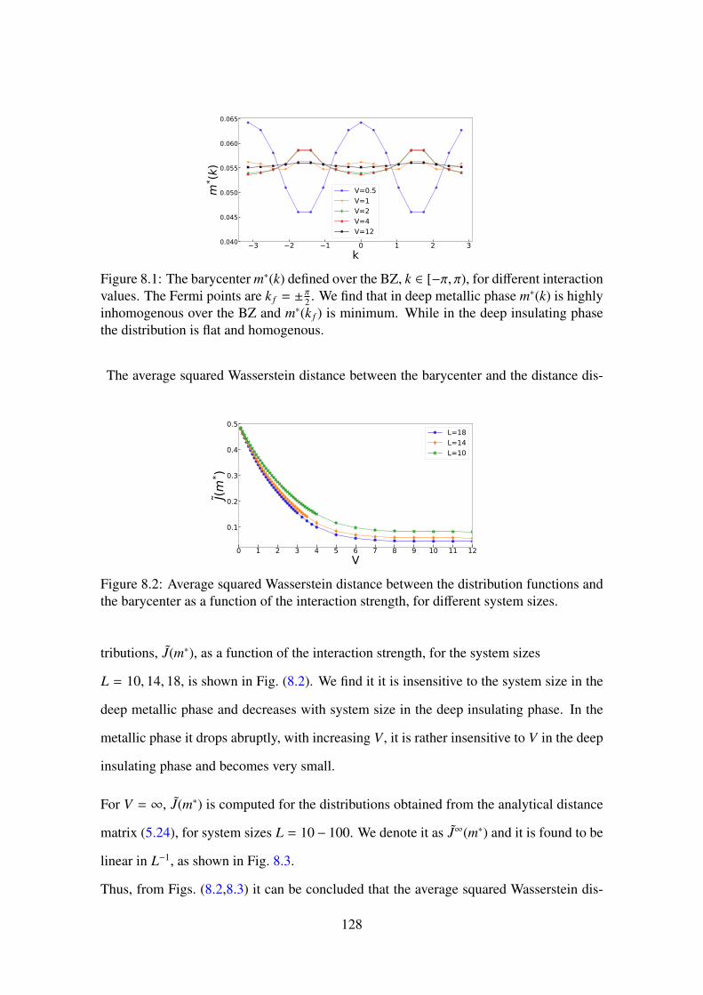
−3 −2 −1 0 1 2 3
k
0.040
0.045
0.050
0.055
0.060
0.065
�*(�
)
V=0.5
V=1
V=2
V=4
V=12
Figure 8.1: The barycenter m∗(k) defined over the BZ, k ∈ [−π, π), for different interactionvalues. The Fermi points are k f = ±π2 . We find that in deep metallic phase m∗(k) is highlyinhomogenous over the BZ and m∗(k f ) is minimum. While in the deep insulating phasethe distribution is flat and homogenous.
The average squared Wasserstein distance between the barycenter and the distance dis-
0 1 2 3 4 5 6 7 8 9 10 11 12
V
0.1
0.2
0.3
0.4
0.5
��
*)
L=18
L=14
L=10
Figure 8.2: Average squared Wasserstein distance between the distribution functions andthe barycenter as a function of the interaction strength, for different system sizes.
tributions, J(m∗), as a function of the interaction strength, for the system sizes
L = 10, 14, 18, is shown in Fig. (8.2). We find it it is insensitive to the system size in the
deep metallic phase and decreases with system size in the deep insulating phase. In the
metallic phase it drops abruptly, with increasing V , it is rather insensitive to V in the deep
insulating phase and becomes very small.
For V = ∞, J(m∗) is computed for the distributions obtained from the analytical distance
matrix (5.24), for system sizes L = 10− 100. We denote it as J∞(m∗) and it is found to be
linear in L−1, as shown in Fig. 8.3.
Thus, from Figs. (8.2,8.3) it can be concluded that the average squared Wasserstein dis-
128

0.00 0.02 0.04 0.06 0.08 0.10
1/�
0.00
0.01
0.02
0.03
0.04
0.05
0.06
0.07
0.08
�∞�
*)
Figure 8.3: Average squared Wasserstein distance between the distribution functions andthe barycenter at the extreme interaction limit, V = ∞ for system sizes L = 10− 100, as afunction of the inverse of system size.
tance between the barycenter and the distance distributions is a single geometric observ-
able which characterises the metallic and insulating phases, because it is non-zero in the
metallic phase and becomes zero in the insulating phase.
129

130
Chapter 9
Ollivier-Ricci Curvature
The intrinsic geometry of the correlated many-body state can be studied by inspecting a
generalisation of the Ricci curvature in a discrete setting. This generalisation, popularly
known as the Ollivier-Ricci curvature, was introduced by Ollivier in the general frame-
work of Markov processes and metric spaces[47, 48]. Later, it was also applied in graph
theory by Lin-Yau[94]. It is also closely connected to Wasserstein distances: in fact, it is
defined in terms of the 1-Wasserstein distances (Eq. (7.12)).
The Ricci curvature has a rich history in geometry: it is a fundamental invariant in Rie-
mannian geometry. In the continuous case, it is a measure of the degree to which the
geometry determined by a given Riemannian metric deviates from that of ordinary Eu-
clidean space. The Ricci curvature is usually the average of sectional curvatures of all
tangent planes with some given direction. It is also closely related to the eigenvalues of
the Laplace-Beltrami operator[95].
Several generalisations of the Ricci curvature in the discrete setting have been at the
center of recent research activities, which not only include the Ollivier-Ricci curvature
but also the Bakry-E’mery curvature[45], the entropic curvature introduced by Erbar
and Maas[49], and the Forman curvature[46]. Lott-Villani-Strum used optimal transport
theory to define the Ricci curvature for metric-measure spaces, using the 2-Wasserstein
131

distances[37].
The above generalisations, being exceedingly simple to study in discrete settings, have
found wide applications in various fields: these include quantum gravity[96, 97], the study
of complex biological networks[98], quantifying the systemic risk and fragility of finan-
cial systems[99], internet topology for the investigation of node degree[100], to name a
few.
Let us examine how this continuous concept was adapted to the discrete setting. The main
intuition used by Ollivier was that the Ricci curvature controls the amount of overlap of
two distance balls in terms of their radii and the distance between their centers[50]. With-
out going into deep technical details, we present a brief sketch of this adaption necessary
for our work.
x y
δw p
w �p�
Figure 9.1: Two nearby balls, m�x and m�y of radius � whose centres are a small distance,δ, apart, along the unit vector v. Parallel transport of a unit vector w gives w� such thatfor a point p ∈ m�x parallel transport along the geodesic of length δ yields a point p� ∈ m�y.The average distance between the points p and p� in flat space is equal to δ, while in thepresence of curvature the lowest-order deviation from δ is given by Equation (9.1).
Let us consider a smooth, N-dimensional Riemannian manifoldM and denote the local
coordinates by xµ, µ = 1, . . . ,N. gµν(x) is the metric. A nearby point with local coordi-
nates y = x + δv is considered, where v is a unit tangent vector at x.
We look at two �-balls, m�x and m�y around x and y which consist of the points inM that
are at a distance ≤ � from x and y respectively.
If m�x is mapped to m�y using the Levi-Civita connection [101], the average distance be-
132

tween the points p ∈ m�x and their images p� ∈ m�y, in the limit δ, � → 0, has been been
shown to be[50],
W(m�x,m�y) = δ
�1 − 1
2(N + 2)κ(v, v) + O(�3 + δ�2)
�. (9.1)
In above equation κ(v, v) is the Ricci curvature associated with the unit vector v. Figure
(9.1) is a schematic illustration.
Extending the above idea to the discrete setting [50, 94] involves replacing the �-ball, m�x
around x by the normalised distribution of distances of all the vertices from the vertex i,
mi( j) =D(i, j)�k D(i, k)
. (9.2)
Moreover, the average distance W is replaced by the 1-Wasserstein distance W(mi,mj)
between two distributions mi and mj. Thus define
W(mi,mj) ≡ infπ
�
kl
D(k, l)πi j(k, l), (9.3)
where πi j(k, l) is a joint probability distribution defined as,
�
l
πi j(k, l) = mi(k),�
k
πi j(k, l) = mj(l). (9.4)
Recall Sec. (7.4) of Chapter 7 where we introduced this distance.
The curvature, κ(i, j), associated with an edge e(i, j) of the graph is then defined by
W(mi,mj) = D(i, j)(1 − κ(i, j)). (9.5)
We can also propose a generalization of the scalar curvature at a point x in Riemannian
manifold, for a graph [95], derived from the Ollivier Ricci curvature defined above. It is
a weak invariant obtained by contracting the Ricci curvature in the Riemannian manifold.
133

The scalar curvature at each vertex i, κ(i), is given by,
κ(i) =1�
k D(i, k)
�
j
κ(i, j). (9.6)
9.1 Results for the t − V model
The curvature along each edge of the graph defined in Equation (9.5) and the scalar cur-
vature defined in Equation (9.6) are computed from the 1-Wasserstein distances obtained
by linear programming and the quantum distance matrix given by exact diagonalization,
for the one-dimensional t − V model. The quasi-momenta (taking values in the BZ),
kl ∈ [−π, π), are given by
kl = −π + 2πlL. (9.7)
With every quasi-momenta mode kl we associate the integer l which runs from 1 to L.
These integers label the vertices of the graph (as per discussions in Sec. (5)).
�� �� �� �� �� �� �� �� ��
k
���
���
���
���
���
���
���
κ�k�k�
��
kf
V��
V��
Figure 9.2: Curvatures for the nearest neighbour edges (k, k + 1) over half the BZ, fordifferent interaction strengths. The integer values of k along the x axis label the verticesof the graph as per Eq. (9.7). The metallic regime is characterised by a discontinuity atthe Fermi point k f .
The values of curvatures in the metallic regime, V � 2, is highly edge-dependent and
they classify the edges into two types, yet again. The edges corresponding to vertices
both inside or outside the FS, e1 ≡ (kin, kin) or (kout, kout), have large curvatures, whereas
134

� � � � � �� ��
V
���
���
���
���
κe�
e�
Figure 9.3: Curvatures for both type of edges e1 and e2 as function of interaction strengthV .
the edges with one of the vertices inside the FS and another one outside it, e2 ≡ (kin, kout)
or (kout, kin), have small curvatures.
The insulating regime, V � 2 (as usual), is characterised by the contrasting behaviour
where curvatures of e1 and e2 are both quite large and uniform.
We have plotted the curvature corresponding to the edges formed by vertices which are
nearest neighbours in the BZ, κ(k, k+1), in Figure (9.2). This figure shows a discontinuity
in the curvature, at the Fermi point which is labelled by k f , for V = 1, in the metallic
regime. This discontinuity decreases smoothly as a function of interaction strength and
disappears at large V . This dip in the curvature at the Fermi point in the metallic regime
is a consequence of the difference in behaviour of the two types of edges. All the nearest
neighbour edges κ(k, k + 1) for k, k + 1 � ±k f belong to e1. In such cases the quantum
distance D(k, k + 1) is small and the distance distributions (Eq. (9.2)) are similar to each
other consequently the Wasserstein distance W(k, k + 1) is small. But the edge with the
Fermi point k f as one of the vertices belongs to e2. The corresponding nearest neighbour
quantum distance is large. The distance distributions are very different, consequently the
Wasserstein distance is large as well. The two distance values don’t differ much from
each other, resulting in small values of curvature as per Eq. (9.5).
Fig. (9.3) shows the Ricci curvature of both types of edges as a function of V . The
curvature of e1 is more or less constant and has a high value at all the values of the
interaction. However, the curvature of e2 continously increases in the metallic and the
135

crossover regime, after which it saturates to a constant high value, roughly the same as
that of e1.
2 4 6 8 10 12 14 16 18
k
0.850
0.875
0.900
0.925
0.950
0.975
1.000
1.025
1.050
1.075
κ(k
)
−kf kf
V=1
V=8
Figure 9.4: Scalar Curvature as a function of the quasi-momenta modes representingvertices of the graph. The integer values along the x axis label the vertices of the graphas per Eq. (9.7). The Fermi points are labelled by ∓k f . In insulating regime the scalarcurvature is uniform over all the vertices.
Fig. (9.4) shows the scalar curvature as a function of the quasi-momenta modes, in the
two regimes. We find the same contrasting behaviour where the insulating phase is char-
acterised by a uniform scalar curvature, whereas in the metallic phase the scalar curvature
varies considerably for different vertices.
From the above results we can conclude the Ollivier-Ricci curvature is able to demarcate
both the phases by a difference in behaviour.
136

Chapter 10
Summary and Outlook
We conclude this thesis by summarizing the findings and presenting future directions of
work that spring from them.
The first half of the thesis introduced a new formalism for studying the quantum geometry
of correlated many-body states. We know the building blocks of many-body states are the
single particle states. The complete set of single particle states can be labelled by some
set of parameters that we have refered to as the spectral parameters.
Our proposition, introduced in Chapter 4, is to define local geometrical observables in the
space of the spectral parameters, in terms of expectation values of appropriately defined
unitary operators. We have succeeded in defining valid quantum distances between pairs
of points in the spectral parameter space that satisfy the triangle inequalities. The defini-
tion gives back the standard quantum distances in the mean-field states as we observed in
Sec. (3.1.1).
The spectral parameters are completely general, they could be quasi-momenta, positions
labelling Wannier orbitals, parameters labelling the eigenfunctions of some confining po-
tential like in a quantum dot or an optical trap. So in parallel to the single-particle for-
malism already well studied in condensed matter system and discussed in Chapter 3, for
137

correlated electron systems we can study local geometrical properties in a space of phys-
ical parameters. Thus we gain over the existing method [9, 18] discussed in Sec. (1.2).
Morever, unlike the single-particle formalism, our theory is capable of probing the quan-
tum geometry of metallic phases as well as insulating ones.
Another advantage of our definition of the distances is, its formulation in terms of ex-
pectation values of the exchange operator. It is thus a purely kinematic definition. So it
gives exclusive geometric characterisation of the ground state, unlike the previous Green’s
function approaches[19, 20, 21, 22, 23, 24] which involved single particle excitations.
Moreover, it can easily be applied to any one-band model. In fact we have applied our
method to the one-dimensional t−V model using exact diagonalization and found striking
results. This model is a one band model exhibiting a Mott transition. So it clearly marks
out these advantages.
The implementation definitely has a wide scope because our definition of the quantum
distances are in terms of the static correlation functions and can be computed applying any
exact or approximate technique like perturbation theory, quantum Monte Carlo methods,
DMRG and bosonisation in one dimension. The static correlation functions of interest
for the one band models are the four-point correlations, while multi-orbital models will
need the computation of higher-order correlation functions. In the same spirit as the
work of Resta and Sorella[29], we have given a geometrical framework for studying the
static correlations, which themselves characterize the many-body states. However, our
correlation functions are slightly different from conventionally studied ones and thus bring
in newer prospects.
The next part of the thesis focused on developing tools to study the quantum distances
and construct geometrical observables from the space of distances. We have a matrix of
quantum distances to begin with, or we can think of this structure as a weighted graph. We
have applied tools popularly used in distance geometry and discrete differential geometry,
for studying the geometry of graphs and networks, which are very popular in other applied
138

fields like computer vision, image processing, data mining, machine learning, the study of
biological networks, finding molecular conformations in NMR, to name only a handful.
We have outlined a method to study the extrinsic geometry of the many-body state by Eu-
clidean embedding of the distances. Even visualization in terms of shapes and surfaces in
lower dimensional Euclidean space was possible by approximate embedding techniques.
A particularly powerful geometric approach has been outlined, by constructing proba-
bility ditributions from the distances and introducing the theory of optimal transport to
study the geometry of these distance distributions. We find geometric observables which
can be obtained by averaging over the space of the spectral parameters. The Wasserstein
distances, which give the distance between the distributions are proposed as geometrical
observables which can capture the phases of the many-body state.
Further, parallel to the localisation tensor, optimal transport theory allows us to define
a single geometric observable characterising the phases by the concept of Wasserstein
barycenter. The average squared Wasserstein distance between the distance distributions
and the barycenter is tracked down as such a geometric observable. This approach to study
the structure of a many-body state is closely related with the machine learning approach
towards data analysis, where one often has to deal with collections of samples that can
be interpreted as probability distributions. One of the fundamental tasks then becomes
comparing, summarising, and reducing the dimensionality of the probability distributions
on a given metric space. In parallel, we generate probability distribution functions from
the many body state and infer geometric properties of ground states by comparing these
distributions (in terms of Wasserstein distance).
A method to study the intrinsic geometry of the many-body state has been proposed as
well, by introducing the Ollivier-Ricci curvature. It is a discrete version of the Ricci
curvature in terms of the Wasserstein distances, and thus has the optimal transport theory
at the heart of its basic construction.
139

10.1 Future plans
This new formalism is at a nascent stage and has a wide scope of applications. Since
much of the motivation comes from the characterisation of the metal-insulator transition
and since our applications to the t − V model succeed in such characterisation by using
the theory of optimal transport, there is the range of applications to other models in order
to find an uniform characterisation.
It will be interesting to bring in the spin degree of freedom and study the Hubbard model,
where the distances can be computed by quantum Monte Carlo. A plan to investigate
the one-dimensional spin chains, applying DMRG to compute the quantum distances, is
under progress.
However, our proposed general scheme is very powerful. We think that if the static cor-
relation functions are computed using any of the exact or approximation techniques (the
ones listed above or even newer ones), we will be able to introduce the geometrical frame-
work of the quantum distances and characterise the phases of any quantum state applying
these new tools.
The distances for conventional tight binding models though are the usual Hilbert-Schmidt
distances, but the above tools can also be used for studying basic physics in such models,
which are well studied by the conventional approach to quantum geometry. Applications
of this new methodology to the Haldane model is also planned for the near future.
Studying the ground state of a system is interesting from the perspective of quantum
phase transitions. The formalism being based on expectation values over a state, it can be
applied to any state in principle and can possibly find applications in dynamical systems
as well.
Coming back to the broader theoretical picture of our formalism, the generalisation of the
140

geometric phases in terms of expectation value of a unitary operator was not possible by
choosing the products of the exchange operators as a candidate. However, there remains
the exciting possibility of finding an appropriate operator such that the additive law is
satisfied.
141

142

Appendix A
Appendix
A.1 Quantum distances of general mean field states
In this section we generalise our previous results of the distance matrix for general mean
field states (MFS).
We consider a general d-dimensional lattice with L unit cells in each direction. We label
the sites of the unit cells by i and the sublattices by a = 1, . . . nB. The sites of the lattice
are denoted by Ria = Ri + ra. Thus Ri specifies a point in the unit cell and ra the locations
of the sub-lattice sites with respect to that point. The fermion creation and annihilation
operators are denoted by (C†ia,Cia). They satisfy the canonical anti-commutation relations.
The Fourier transforms of these operators are defined as,
Ca(k) ≡ 1
Ld2
�
i
eik·RiaCia (A.1)
where k ∈ BZ.
We denote the single-particle hamiltonian in the quasi-momentum space by hab(k) and its
spectrum by,
hab(k)unb(k) = �n(k)un
a(k). (A.2)
143

We denote the Fermi level by �F and the number of occupied bands at k by NF(k), namely,
NF(k) ≡NB�
n=1
Θ (�F − �n(k)) . (A.3)
The general mean field state is defined as
|u, �F� ≡�
k
NF (k)�
n=1
�un
a(k)C†a(k)�|0� (A.4)
where u denotes the full set of eigenstates, un(k). We define Ψa1,...aN(k) (k) to be the anti-
symmetrised product of the NF(k) single particle wave functions, un(k),
Ψa1...aNF (k) (k) =�
P
(−1)PNF (k)�
l=1
un(k)aP(l) (A.5)
The general mean field state can be written in the factorised form,
|Ψ(k)� ≡�
a
Ψa1...aNF (k) (k)NF (k)�
l=1
C†al(k)
|0�k
|u, �F� =�
k
|Ψ(k)� (A.6)
where�
a denotes the sum over all the nBCNF (k) combinations of the the index a and�
k
denotes the direct product of the states defined at each point in the BZ.
A.1.1 The quantum distance matrix
Our definition of the quantum distance matrix is,
D2(k1, k2) ≡ 1 − |�u, �F |E(k1, k2)|u, �F�|α (A.7)
144

where E(k1, k2) are the exchange operators. They are unitary operators and their action
of the fermion creation operators is given by,
E(k1, k2)C†a(k1)E†(k1, k2) = ±C†a(k2) (A.8)
E(k1, k2)C†a(k2)E†(k1, k2) = ±C†a(k1). (A.9)
The ± signs above depend on the ordering convention of the creation operators in the
definition of the many-body states. While it is important to keep track of them for cor-
related states, as we will see below, due to the factorized form of MFS, the distances are
independent of the signs.
The action of the exchange operator on the states is
E(k1, k2)|ψ(k1)� ⊗ |ψ(k2)� = ±�
aa�Ψa1...aNF (k1) (k1)
Ψa�1...a�NF (k2)
(k2)�
NF (k2)�
l�=1
C†a�l (k2)|0�k2
⊗NF (k1)�
l=1
C†al(k1)|0�k1 .
(A.10)
Equations (A.7), (A.8), (A.9) and (A.10) imply
D2(k1, k2) = 1 − |�Ψ(k1))|Ψ(k2))�|2α δNF (k1),NF (k2). (A.11)
For α = 1, the RHS of the above equation is the Hilbert- Schmidt distance between Ψ(k1)
andΨ(k2). Thus we have shown that the quantum distances of the mean field states reduce
to the standard definition in terms of the overlap of wavefunctions. For α = 1, it is exactly
the Hilbert-Schmidt distance between the NF(k) states at k. Our definition also implies
145

that the distance between two quasi-momenta with different occupation numbers is equal
to 1.
A.2 The classical Ptolemy problem for α = 2
In this section we look at the special case α = 2 in the definition of distances in Eq. (4.9).
This case is special in the sense, the proof of the triangle inequalities is interesting in this
case. We encounter the classical Ptolemy problem in 3-dimensional Euclidean space.
To state the problem, we are given four normalized vectors in a Hilbert space,H , |χµ�, µ =0, . . . , 3. Let |ψ� ≡ |χ0� denote the correlated many-body state being studied. The remain-
ing three states are the states generated by the action the exchange operators (introduced
in Chapter 4) on it. The six distances between these four vectors are given by,
Dµν =�
1 − |�χµ|χν�|2 (A.12)
We will now prove that we can always find 4 points in a 3-dimensional Euclidean space,
�xµ, such that,
Dµν = |�xµ − �xν| (A.13)
This reduces the problem to the classical Ptolemy problem.
We can always find a 4-dimensional subspace ofH which contains the four vectors, |χµ�.The physical states, forming the manifold CP3, are in one-to-one correspondence with the
pure state density matrices,
ρµ ≡ |χµ��χµ|. (A.14)
The distances defined in Eq. (A.12) can be expressed as,
Dµν =�
1 − Tr( ρµρν ) (A.15)
146

Since ρµ are hermitian, they can be expressed as a linear combination, with real coef-
ficients, of the identity matrix and the 15 generators of S U(4) in the fundamental rep-
resentation. We denote them by, Tα, α = 1, . . . , 15. They can always be chosen such
that,
TrTα = 0, TrTαTβ = δαβ (A.16)
Thus we have,
ρµ = a0I +15�
α=1
aαµTα (A.17)
a0 =14
Trρµ (A.18)
aαµ = TrTαρµ (A.19)
The fact that, Trρ2µ = Trρµ = 1 implies that,
a0 =14, �aµ · �aµ ≡
15�
α=1
aαµaαµ = 1 − 1
16=
1516
(A.20)
Note that ρ2µ = ρµ implies other constraints on �a, but these are not relevant for our proof.
Thus, we have shown that each of the physical states, ρµ, can be represented by a point on
a 14-dimensional sphere of radius√
154 .
The distance Dµν can be expressed in terms of �aµ,
D2µν = 1 − Tr(ρµρν)
=1516− �aµ · �aν
=12|�aµ − �aν|2 (A.21)
Thus, if we define �xµ ≡ 1√2�aµ, then we have constructed four points, �xµ, in a 15-dimensional
147
Euclidean space such that the 6 distances between them are Dµν. Namely,
D2µν = |�xµ − �xν|2 (A.22)
We can always find a 3-dimensional subspace of this 15-dimensional Euclidean space that
contains the four points �xµ.
Hence, we have found 4 points, �xµ in a 3-dimensional Euclidean vector space such that
the 6 distances between them is Dµν. Thus the problem reduces to the classical Ptolemy
problem.
A.3 Optimal transport problem at the extreme interac-
tion limits
In this section, we present analytic proofs for the results stated in the text (Eq. s 7.19) for
W(mi,mj) in the extreme limits of the coupling. Namely, V = 0 and V = ∞.
A.3.1 V = 0
The distance matrix at V = 0 can be written as
D =
0 II 0
(A.23)
where I is the L/2×L/2 matrix with all entries equal to 1. We denote the L/2 component
column vector with all entries equal to 1 by e. We represent the distance distributions
148

defined in Equation 5.8 by column vectors mi,mL/2+i, i = 1, . . . , L/2,
mi =2L
0
e
mL/2+i =2L
e
0
. (A.24)
The constraints defining the joint probability distributions, πi j can be writen in a matrix
form,
πi j
e
e
= mi
�eT eT
�πi j = mT
j (A.25)
The general solution to the above equations(A.25) is
πi j =2L
0 0
0 P
πiL/2+ j =2L
0 0
P 0
πL/2+i j =2L
0 P
0 0
πL/2+iL/2+ j =2L
P 0
0 0
,
where i, j = 1, . . . , L/2. P is any L/2 × L/2 component positive semi-definite matrix
whose rows and columns sum up to 1. P(i, j) ≥ 0,�L/2
k=1 P(k, l) = 1 =�L/2
l=1 P(k, l).
The Wasserstein distances can be written in this matrix form as,
W(mi,mj) = infπ
Tr�D(2)πi j
�, (A.26)
where D(2)(k, l) = (D(k, l))2. Using the fact that PI = I = IP, it is easy to see that
the RHS of the above equation is independent of P and we obtain the result stated in
equation(7.19), that at V = 0,
W(mi,mj) = (D(i, j))2 (A.27)
149

A.3.2 V = ∞
The distance matrix in the limit V = ∞ for α = 2 is
D = c
I − I II I − I
+ (1 − c)
0 I
I 0
, (A.28)
where c =√
3/2. To represent the distance distributions as column vectors, we define a
set of L/2 component column vectors, χi, i = 1, . . . , L/2 whose entries are all zero except
for the ith one, which is equal to 1. Namely, χi( j) = δi j. We then have,
mi =1L
ce − cχi
ce + (1 − c)χi
, mL/2+i =1L
ce + (1 − c)χi
ce − cχi
(A.29)
where L = c(L − 2) + 1. We present a set of solutions to equations. We have no proof
that these are the most general solutions. However, the definition of the Wasserstein
distance in equation(A.26) implies that the infimum in this set provides an upper bound
for W(mi,mj). The solutions are of the form,
πi j =1L
�cPi j + π
�i j
�(A.30)
where Pi j are L × L, positive semi-definite matrices whose columns and rows sum up to
1.
Pi j ≥ 0,L�
k=1
Pi j(k, l) = 1 =L�
l=1
Pi j(k, l) (A.31)
150

π�i j are,
π�i j =
−cχiχ
Tj 0
0 (1 − c)χiχTj
π�iL/2+ j =
0 −cχiχ
Tj
(1 − c)χiχTj 0
π�L/2+i j =
0 (1 − c)χiχ
Tj
−cχiχTj 0
π�L/2+iL/2+ j =
(1 − c)χiχ
Tj 0
0 −cχiχTj
. (A.32)
Equations (A.30), (A.32) and the constraint πi j(k, l) ≥ 0, k, l = 1, . . . , L, implies that
Pi j(i, j) − 1 ≥ 0. Since the maximum value of the matrix elements of Pi j is 1, we have,
Pi j(i, j) = 1, Pi j(i, k) = 0 ∀k � j, Pi j(k, j) = 0 ∀k � i. (A.33)
Consider the set of matrices, P∗i j defined as,
P∗i j(k, l) ≡ δkl
�1 − δik − δ jl
�+ δikδ jl + δilδ jk, (A.34)
it is straightforward to verify that P∗i j satisfy all the constraints in equations (A.31) and
(A.33).
Thus, equations (A.26) and (A.30) imply,
W(mi,mj) ≤ 1LTr
�D(2)
�cP∗i j + π
�i j
��. (A.35)
The RHS of the above inequality can be computed using equations (A.28), (A.32) and
151

(A.34). The result is,
Tr�D(2)
�cP∗i j + π
�i j
��= (D(i, j))2 (A.36)
Thus, we have proved the result stated in equation 7.19, that at V = ∞,
W(mi,mj) ≤ 1L (D(i, j))2. (A.37)
152

Bibliography
[1] M. V. Berry, “Quantal phase factors accompanying adiabatic changes,” Proceed-
ings of the Royal Society of London. A. Mathematical and Physical Sciences,
vol. 392, no. 1802, pp. 45–57, 1984.
[2] D. J. Thouless, M. Kohmoto, M. P. Nightingale, and M. den Nijs, “Quantized Hall
conductance in a two-dimensional periodic potential,” Phys. Rev. Lett., vol. 49,
pp. 405–408, Aug 1982.
[3] J. E. Avron, R. Seiler, and B. Simon, “Homotopy and quantization in condensed
matter physics,” Phys. Rev. Lett., vol. 51, pp. 51–53, Jul 1983.
[4] Q. Niu and D. J. Thouless, “Quantised adiabatic charge transport in the presence of
substrate disorder and many-body interaction,” Journal of Physics A: Mathematical
and General, vol. 17, pp. 2453–2462, aug 1984.
[5] F. D. M. Haldane, “Model for a Quantum Hall Effect without Landau Levels:
Condensed-Matter Realization of the "Parity Anomaly",” Phys. Rev. Lett., vol. 61,
pp. 2015–2018, Oct 1988.
[6] R. Karplus and J. M. Luttinger, “Hall Effect in Ferromagnetics,” Phys. Rev., vol. 95,
pp. 1154–1160, Sep 1954.
[7] G. Sundaram and Q. Niu, “Wave-packet dynamics in slowly perturbed crystals:
Gradient corrections and Berry-phase effects,” Phys. Rev. B, vol. 59, pp. 14915–
14925, Jun 1999.
153

[8] F. D. M. Haldane, “Quantum geometry in conducting systems,” June 2006. PIT P-
Les Houches Summer School, Quantum Magnetism.
[9] D. Xiao, M.-C. Chang, and Q. Niu, “Berry phase effects on electronic properties,”
Rev. Mod. Phys., vol. 82, pp. 1959–2007, Jul 2010.
[10] F. D. M. Haldane, “Berry Curvature on the Fermi Surface: Anomalous Hall Effect
as a topological Fermi-liquid property,” Phys. Rev. Lett., vol. 93, p. 206602, Nov
2004.
[11] R. D. King-Smith and D. Vanderbilt, “Theory of polarization of crystalline solids,”
Phys. Rev. B, vol. 47, pp. 1651–1654, Jan 1993.
[12] R. Resta, “Macroscopic polarization in crystalline dielectrics: the geometric phase
approach,” Rev. Mod. Phys., vol. 66, pp. 899–915, Jul 1994.
[13] R. Resta, “The insulating state of matter: a geometrical theory,” The European
Physical Journal B, vol. 79, pp. 121–137, Jan 2011.
[14] F. D. M. Haldane, “Topology and geometry in quantum condensed matter.”
PCCM/PCTS Summer School, July 2012.
[15] N. Mukunda and R. Simon, “"quantum kinematic approach to the geometric phase.
i. general formalism",” Annals of Physics, vol. 228, no. 2, pp. 205 – 268, 1993.
[16] V. Bargmann, “Note on Wigner’s theorem on symmetry operations,” Journal of
Mathematical Physics, vol. 5, no. 7, pp. 862–868, 1964.
[17] R. Simon and N. Mukunda, “Bargmann invariant and the geometry of the Güoy
effect,” Phys. Rev. Lett., vol. 70, pp. 880–883, Feb 1993.
[18] I. Souza, T. Wilkens, and R. M. Martin, “Polarization and localization in insulators:
Generating function approach,” Phys. Rev. B, vol. 62, pp. 1666–1683, Jul 2000.
154

[19] Z. Wang, X.-L. Qi, and S.-C. Zhang, “Topological Order Parameters for Interacting
Topological Insulators,” Phys. Rev. Lett., vol. 105, p. 256803, Dec 2010.
[20] Z. Wang and S.-C. Zhang, “Simplified Topological Invariants for Interacting Insu-
lators,” Phys. Rev. X, vol. 2, p. 031008, Aug 2012.
[21] L. Wang, X. Dai, and X. C. Xie, “Frequency domain winding number and interac-
tion effect on topological insulators,” Phys. Rev. B, vol. 84, p. 205116, Nov 2011.
[22] V. Gurarie, “Single-particle Green’s functions and interacting topological insula-
tors,” Phys. Rev. B, vol. 83, p. 085426, Feb 2011.
[23] K.-T. Chen and P. A. Lee, “Unified formalism for calculating polarization, magne-
tization, and more in a periodic insulator,” Phys. Rev. B, vol. 84, p. 205137, Nov
2011.
[24] Z. Wang, X.-L. Qi, and S.-C. Zhang, “Topological invariants for interacting topo-
logical insulators with inversion symmetry,” Phys. Rev. B, vol. 85, p. 165126, Apr
2012.
[25] W. Kohn, “Theory of the insulating state,” Phys. Rev., vol. 133, pp. A171–A181,
Jan 1964.
[26] L. D. Landau, “On the theory of phase transitions,” Zh. Eksp. Teor. Fiz., vol. 7,
pp. 19–32, 1937. [Ukr. J. Phys.53,25(2008)].
[27] R. Resta, “Quantum-mechanical position operator in extended systems,” Phys. Rev.
Lett., vol. 80, pp. 1800–1803, Mar 1998.
[28] R. Resta, “Why are insulators insulating and metals conducting?,” Journal of
Physics: Condensed Matter, vol. 14, no. 20, p. R625, 2002.
[29] R. Resta and S. Sorella, “Electron localization in the insulating state,” Phys. Rev.
Lett., vol. 82, pp. 370–373, Jan 1999.
155

[30] R. Resta, “Electron Localization in the Quantum Hall Regime,” Phys. Rev. Lett.,
vol. 95, p. 196805, Nov 2005.
[31] R. Resta, “Why are insulators insulating and metals conducting?,” Journal of
Physics: Condensed Matter, vol. 14, no. 20, p. R625, 2002.
[32] C. Sgiarovello, M. Peressi, and R. Resta, “Electron localization in the insulating
state: Application to crystalline semiconductors,” Phys. Rev. B, vol. 64, p. 115202,
Aug 2001.
[33] C. N. Yang and C. P. Yang, “One-dimensional chain of anisotropic spin-spin inter-
actions. I. proof of Bethe’s hypothesis for ground state in a finite system,” Phys.
Rev., vol. 150, pp. 321–327, Oct 1966.
[34] R. J. Baxter, Exactly Solved Models in Statistical Mechanics. Academic Press,
1982.
[35] M. A. Cazalilla, R. Citro, T. Giamarchi, E. Orignac, and M. Rigol, “One dimen-
sional bosons: From condensed matter systems to ultracold gases,” Rev. Mod.
Phys., vol. 83, pp. 1405–1466, Dec 2011.
[36] I. J. Schoenberg, “On Metric Arcs of Vanishing Menger Curvature,” Annals of
Mathematics, vol. 41, no. 4, pp. 715–726, 1940.
[37] J. Lott and C. Villani, “Ricci curvature for metric-measure spaces via optimal trans-
port.,” Ann. Math. (2), vol. 169, no. 3, pp. 903–991, 2009.
[38] S. Ohta Comment. Math. Helv, vol. 82, pp. 805–828, 2007.
[39] K.-T. Sturm, “On the geometry of metric measure spaces. ii,” Acta Math., vol. 196,
no. 1, pp. 133–177, 2006.
[40] E. Saucan, Metric Curvatures Revisited: A Brief Overview, pp. 63–114. 10 2017.
156

[41] K. F. Gauss, “General investigations of curved surfaces of 1827 and 1825,” Nature,
vol. 66, pp. 316–317, 2010.
[42] E. Saucan and E. Appleboim, “Curvature Based Clustering for DNA Microarray
Data Analysis,” pp. 405–412, 06 2005.
[43] A. Wald, “Sur la courbure des surfaces,” C. R. Acad. Sci. Paris, vol. 201, pp. 918–
920, 1935.
[44] A.-I. Bonciocat and K.-T. Sturm, “Mass transportation and rough curvature bounds
for discrete spaces,” Journal of Functional Analysis, vol. 256, no. 9, pp. 2944 –
2966, 2009.
[45] D. Bakry and M. Émery, “Diffusions hypercontractives,” in Séminaire de Probabil-
ités XIX 1983/84 (J. Azéma and M. Yor, eds.), (Berlin, Heidelberg), pp. 177–206,
Springer Berlin Heidelberg, 1985.
[46] R. Forman, “Bochner’s method for cell complexes and combinatorial Ricci curva-
ture,” Discrete and Computational Geometry, vol. 29, pp. 323–374, 2003.
[47] Y. Ollivier, “Ricci curvature of Markov chains on metric spaces,” Journal of Func-
tional Analysis, vol. 256, no. 3, pp. 810 – 864, 2009.
[48] Y. Ollivier, “A survey of Ricci curvature for metric spaces and Markov chains,”
Probabilistic Approach to Geometry, vol. 57, 01 2010.
[49] M. Erbar and J. Maas, “Ricci curvature of finite Markov chains via convexity of
the entropy,” Archive for Rational Mechanics and Analysis, vol. 206, pp. 997–1038,
Dec 2012.
[50] Y. Ollivier, A visual introduction to Riemannian curvatures and some discrete gen-
eralizations. AMS, 2013.
[51] L. Liberti and C. Lavor, “Six mathematical gems from the history of distance ge-
ometry,” International Transactions in Operational Research, vol. 23, 02 2015.
157

[52] L. Liberti, C. Lavor, N. Maculan, and A. Mucherino, “Euclidean distance geometry
and applications,” SIAM Review, vol. 56, 05 2012.
[53] I. Dokmanic, R. Parhizkar, J. Ranieri, and M. Vetterli, “Euclidean distance
matrices: A short walk through theory, algorithms and applications,” CoRR,
vol. abs/1502.07541, 2015.
[54] I. J. Schoenberg, “Remarks to Maurice Frechet’s Article “Sur La Definition
Axiomatique D’Une Classe D’Espace Distances Vectoriellement Applicable Sur
L’Espace De Hilbert,” Annals of Mathematics, vol. 36, no. 3, pp. 724–732, 1935.
[55] T. Crilly, “The rise of Cayley’s invariant theory (1841−1862),” Historia Mathemat-
ica, vol. 13, no. 3, pp. 241 – 254, 1986.
[56] K. Menger, “Untersuchungen über allgemeine Metrik,” Mathematische Annalen,
vol. 100, pp. 75–163, Dec 1928.
[57] Bluemental, Theory and Applications of Distance Geometry. Oxford University
Press, 1953.
[58] P. Indyk and J. Matousek, Low-Distortion Embeddings of Finite Metric Spaces.
CRC Press, 2004.
[59] Y. Rabinovich, “On average distortion of embedding metrics into the line and into
l1,” pp. 456–462, 2003.
[60] I. Abraham, Y. Bartal, and O. Neiman, “Advances in metric embedding theory,”
Advances in Mathematics, vol. 228, no. 6, pp. 3026 – 3126, 2011.
[61] R. Gemulla and P. Miettinen, “Data mining and matrices,03− singular value de-
composition,” 2013. Lecture slides Max Planck Institut Informatik.
[62] T. M. Mitchell, “Reducing data dimension,” 2005. Lecture slides on Machine
Learning, Carnegie Mellon University.
158

[63] C. Villani, Optimal Transport: Old and New. Grundlehren der mathematischen
Wissenschaften, Springer, 2009 ed., Sept. 2008.
[64] C. Villani, Topics in Optimal Transportation. Graduate studies in mathematics,
American Mathematical Society, 2003.
[65] S. Kolouri, S. R. Park, M. Thorpe, D. Slepcev, and G. K. Rohde, “Optimal mass
transport: Signal processing and machine-learning applications,” IEEE Signal Pro-
cessing Magazine, vol. 34, pp. 43–59, July 2017.
[66] M. Agueh and G. Carlier, “Barycenters in the Wasserstein Space,” SIAM Journal
on Mathematical Analysis, vol. 43, no. 2, pp. 904–924, 2011.
[67] M. Cuturi, “Sinkhorn distances: Lightspeed computation of optimal transport,” in
Proceedings of the 26th International Conference on Neural Information Process-
ing Systems - Volume 2, NIPS’13, (USA), pp. 2292–2300, Curran Associates Inc.,
2013.
[68] M. Arjovsky, S. Chintala, and L. Bottou, “Wasserstein generative adversarial net-
works,” in Proceedings of the 34th International Conference on Machine Learning
(D. Precup and Y. W. Teh, eds.), vol. 70 of Proceedings of Machine Learning Re-
search, (International Convention Centre, Sydney, Australia), pp. 214–223, PMLR,
06–11 Aug 2017.
[69] N. Courty, R. Flamary, D. Tuia, and A. Rakotomamonjy, “Optimal transport for
domain adaptation,” CoRR, vol. abs/1507.00504, 2015.
[70] G. Buttazzo, L. De Pascale, and P. Gori-Giorgi, “Optimal-transport formulation of
electronic density-functional theory,” Phys. Rev. A, vol. 85, p. 062502, Jun 2012.
[71] C. Cotar, G. Friesecke, and C. Kluppelberg, “Density functional theory and op-
timal transportation with Coulomb cost,” Communications on Pure and Applied
Mathematics, vol. 66, no. 4, pp. 548–599, 2013.
159

[72] M. Cuturi and A. Doucet, “Fast Computation of Wasserstein Barycenters,” in Pro-
ceedings of the 31st International Conference on Machine Learning (E. P. Xing
and T. Jebara, eds.), vol. 32 of Proceedings of Machine Learning Research, (Be-
jing, China), pp. 685–693, PMLR, 22–24 Jun 2014.
[73] J. M. Luttinger, “An exactly soluble model of a many-Fermion system,” Journal of
Mathematical Physics, vol. 4, no. 9, pp. 1154–1162, 1963.
[74] F. D. M. Haldane, “General relation of correlation exponents and spectral prop-
erties of one-dimensional Fermi Systems: application to the anisotropic S = 12
Heisenberg chain,” Phys. Rev. Lett., vol. 45, pp. 1358–1362, Oct 1980.
[75] F. D. M. Haldane, “’Luttinger liquid theory’ of one-dimensional quantum fluids. I.
Properties of the Luttinger model and their extension to the general 1D interacting
spinless Fermi gas,” Journal of Physics C: Solid State Physics, vol. 14, no. 19,
p. 2585, 1981.
[76] R. Shankar, “Solvable model of a metal-insulator transition,” International Journal
of Modern Physics B, vol. 04, no. 15n16, pp. 2371–2394, 1990.
[77] K. Gödel, K. Gödel Collected Works. Oxford University Press: Oxford, 1953.
[78] W. Braun, “Distance geometry and related methods for protein structure determina-
tion from NMR data,” Quarterly Reviews of Biophysics, vol. 19, no. 3-4, pp. 115–
157, 1987.
[79] G. H. Forman and J. Zahorjan, “The challenges of mobile computing,” Computer,
vol. 27, pp. 38–47, Apr. 1994.
[80] G. Saporta, “The analysis of proximity data. b. s. everitt and s. rabe-hesketh, arnold,
london, 1997,” Statistics in Medicine, vol. 18, no. 4, pp. 491–492, 1999.
[81] G. Monge, “Memoire sur la theorie des deblais et des remblais,” In Histoire de
lAcademie Royale des Sciences de Paris, pp. 666–704, 1781.
160

[82] L. V. Kantorovich, “On translocation of masses,” USSR AS Doklady. New Serie.,
vol. 37, pp. 227–229, 1942.
[83] Y. Rubner, C. Tomasi, and L. J. Guibas, “The earth mover’s distance as a metric for
image retrieval,” International Journal of Computer Vision, vol. 40, pp. 99–121,
Nov 2000.
[84] K. Ni, X. Bresson, T. Chan, and S. Esedoglu, “Local histogram based segmentation
using the Wasserstein distance,” International Journal of Computer Vision, vol. 84,
pp. 97–111, Aug 2009.
[85] “A probability metrics approach to financial risk measures, by svetlozar t. rachev,
stoyan v. stoyanov, and frank j. fabozzi, 2011, oxford, uk: Wiley blackwell, 392 pp.
isbn: 978-1-4051-8369-7,” Journal of Risk and Insurance, vol. 83, no. 2, pp. 505–
510, 2016.
[86] K.-T. Sturm, “Probability measures on metric spaces of nonpositive curvature, heat
kernels and analysis on manifolds,” Graphs, and Metric Spaces, pp. 357–390, 01
2002.
[87] R. Sinkhorn and P. Knopp, “Concerning nonnegative matrices and doubly stochas-
tic matrices.,” Pacific J. Math., vol. 21, no. 2, pp. 343–348, 1967.
[88] P. A. Knight, “The sinkhorn-knopp algorithm: Convergence and applications,”
SIAM J. Matrix Anal. Appl., vol. 30, pp. 261–275, Mar. 2008.
[89] M. Cuturi and A. Doucet, “Fast computation of Wasserstein barycenters,” in Pro-
ceedings of the 31st International Conference on Machine Learning (E. P. Xing
and T. Jebara, eds.), vol. 32 of Proceedings of Machine Learning Research, (Be-
jing, China), pp. 685–693, PMLR, 22–24 Jun 2014.
161

[90] J.-D. Benamou, G. Carlier, M. Cuturi, L. Nenna, and G. Peyré, “Iterative Bregman
Projections for Regularized Transportation Problems,” SIAM Journal on Scientific
Computing, vol. 2, no. 37, pp. A1111–A1138, 2015.
[91] J. Solomon, F. de Goes, G. Peyré, M. Cuturi, A. Butscher, A. Nguyen, T. Du, and
L. Guibas, “Convolutional Wasserstein distances: efficient optimal transportation
on geometric domains,” ACM Trans. Graph., vol. 34, pp. 66:1–66:11, July 2015.
[92] B. Muzellec and M. Cuturi, “Generalizing point embeddings using the Wasserstein
space of elliptical distributions,” in Proceedings of the 32Nd International Confer-
ence on Neural Information Processing Systems, NIPS’18, 2018.
[93] H. Xu, W. Wang, W. Liu, and L. Carin, “Distilled Wasserstein learning for word
embedding and topic modeling,” CoRR, vol. abs/1809.04705, 2018.
[94] Y. Lin, L. Lu, and S.-T. Yau 2011.
[95] J. Jost and S. Liu, “Ollivier’s Ricci curvature, local clustering and curvature-
dimension inequalities on graphs,” Discrete Comput. Geom., vol. 51, pp. 300–322,
Mar. 2014.
[96] C. A. Trugenberger, “Random holographic “large worlds” with emergent dimen-
sions,” Phys. Rev. E, vol. 94, p. 052305, Nov 2016.
[97] C. A. Trugenberger, “Combinatorial quantum gravity: geometry from random
bits,” Journal of High Energy Physics, vol. 2017, p. 45, Sep 2017.
[98] R. P. Sreejith, J. Jost, E. Saucan, and A. Samal, “Forman curvature for directed
networks,” 2016.
[99] R. S. Sandhu, T. T. Georgiou, and A. R. Tannenbaum, “Ricci curvature: An eco-
nomic indicator for market fragility and systemic risk,” Science Advances, vol. 2,
no. 5, 2016.
162

[100] C.-C. Ni, Y.-Y. Lin, J. Gao, X. Gu, and E. Saucan, “Ricci curvature of the internet
topology,” 2015 IEEE Conference on Computer Communications (INFOCOM),
pp. 2758–2766, 2015.
[101] M. d. T. Levi-Civita, “Nozione di parallelismo in una varietà qualunque e con-
seguente specificazione geometrica della curvatura riemanniana,” Rendiconti del
Circolo Matematico di Palermo (1884-1940), vol. 42, pp. 173–204, Dec 1916.
163


