Rating Banks:Risk and Uncertainty in an Opaque Industry
Donald P. Morgan*April 2000
AbstractThe pattern of disagreement between bond raters suggests that bank and insurance
firms are inherently more opaque than other firms. Moody’s and S&P split more frequently over thesefinancial intermediaries and the splits are more lopsided, as theory here predicts. Uncertainty over thebanks stems from their assets, loans and trading assets in particular, the risks of which are hard toobserve or easy to change. Banks’ high leverage, which invites agency problems, compounds theuncertainty over their assets. Our findings bear on both the existence and reform of bank regulation.
JEL Codes: G20, G21, G28.
__________________*Federal Reserve Bank of New York. [email protected]. Earlier version of this paper circulated as “Whetherand Why Banks are Opaque,” and “Rating Banks: Why Can’t Raters Agree?” The views in this paper do notnecessarily represent those of the Federal Reserve Bank of New York or the Federal Reserve System. For theirhelpful comments, I thank Richard Cantor, Becky Demsetz, Mark Flannery, Chris James, George Kaufmann, JamieMcAndrews, Robert Rich, Frank Packer, Ellerie Weber, and seminar participants at the Federal Reserve Bank of New

2
York, the Federal Reserve Bank of St. Louis, the Bank of England, the Riksbank (Stockholm), and CEMFI (Madrid).Thanks also to Leslie Dupuy for research assistance.
3
Introduction
Why do we regulate and protect banks? Why not leave it to the savers and investors who put
their money in banks? The regulators’ rationale goes something like this. Banks are black boxes:
money goes in, and money goes out, but the risks taken in the process of intermediation are hard to
observe from outside the bank. Absent the steadying hand of government--deposit and payments
insurance, lender of last resort, supervision and regulation of bank risk taking--the opacity of banks
exposes the entire financial system to bank runs, contagion, and other strains of “systemic” risk.
Take away opacity and the whole story unravels. Were banks as transparent as other firms,
runs on “risky” banks would never infect the “safe” ones and the preventative of deposit insurance
would be unnecessary. Without deposit insurance and the excessive risk taking it invites, government
supervision and regulation of banks would also redundant; that role could be left to the market. Nor
would we need a discount window and lender of last resort, since fully transparent banks could borrow
at open market rates that fairly reflected the their risk.1
As yet, opacity is more presumption than fact. There seems not to be a single piece of evidence
suggesting banking firms are somehow harder to fathom any other sort of firm.2 The issue looms even
larger today as regulators from around the world consider the reform of the regulatory structure of
banks. Among the proposed “pillars” of reform are increased market discipline of banks, via
mandatory issuance of subordinated debt by banks or their holding companies, and increased
transparency of banks, via increased disclosure. Given the presumed opacity of banks, how strong are
these pillars? How much of the burden of bank discipline can supervisors expect to shift to the market?
Can banks become transparent, or is opacity to some degree inherent to the business?
1Even the link between monetary policy and bank lending depends on how accurately the market can observe therisk of banks. When the Fed drains reserves, banks could maintain their lending by issuing uninsured debt that doesnot require reserves, such as large CDS or debentures. (Romer and Romer 1990). But if that debt is mispriced(because investors cannot observe the risk of banks), better banks will reduce their lending following a tightening inmonetary policy (Stein 1995).
2 Flannery et al (1999) is the only other paper that even takes up the issue and their conclusion, based on thetrading patterns of matched pairs of banks and non-banks, is largely negative: “. . . justifying special treatment ofbanking firms requires some market failure other than extreme opacity” (p. 25).
4
This paper investigates the relative opacity of banks using disagreement between the major
bond rating agencies--Moody’s and S&P--as a proxy for uncertainty.3 The empirical strategy is
simple. If the supposed opacity of banks makes their risk harder to quantify, we should observe more
frequent and wider disagreement over banks’ bonds. The only subtlety is whether to expect the splits
should be symmetric, or lopsided, with one or the other agency lower on average. Using a simple
model, we show that the greater uncertainty in more opaque sectors will lead to more lopsided splits, at
least if one agency tends to rate more conservatively in general. Intuitively, the heightened uncertainty in
more opaque sectors implies more risk of overrating and underrating, but since the conservative rater
worries more about overrating (by definition), he errs further on the safe side in the more opaque
sectors.
From a policy perspective, it is also important to understand the source of uncertainty over
banks. Is opacity inherent to banking, in which case intervention might be justified, or is opacity the
result of intervention? There is the view that deposit insurance, the discount window, and the occasional
bank bailout have made banks opaque by protecting them from market discipline. From this
perspective, the veil between banks and the market is simply the downside of the government safety net.
The timing of disagreement we find between raters is suggestive on this point, but not definitive.
Splits over banks-- big banks especially-- increased markedly after 1986 and the demise of “too big to
fail” (Flannery and Sorescu 1990). While this timing makes sense, it forces the question: was it the
banks themselves raters were increasingly unsure about after 1986, or was it the regulators and their
commitment to the new laissez faire policy?
Intermediation and agency theory point to the unique mix of assets and leverage at banks as a
source of fundamental uncertainty about bank risk.4 As “delegated monitors,” banks are supposed to
3 Disagreement between forecasters has been used to gauge uncertainty about macroeconomic variables. Seecitations in Bomberger (1996). Opacity, with its underlying premise of informational asymmetries, seems more closelyrelated to “uncertainty” as in Knight (1921), than to risk.
4A classic text for financial analysts puts it this way: “Probably in no other field involving such large public interestsis there more uncertainty for the investor (than in banking). .. partly because of the difficulty in valuing loans anddiscounts...and partly because... any fluctuation in the value of the assets bulk so large for the small net worth.”(Guthman 1953, p. 494)
5
lend to less known borrowers requiring intensive screening and monitoring (Diamond 1983). Lending to
opaque borrowers, however, may cause opaque banks. The trading assets at the money center banks
in the U.S. may be another source of uncertainty. These assets are not necessarily opaque in the same
way loans are, but they are extremely liquid and hence “slippery;” trading positions are easily and
instantaneously changed, which makes them hard to monitor. Trading, as Myers and Ragan (1997) put
it, is the “dark side” of liquidity for banks. The high leverage at banks may compound the uncertainty
over their assets; their assets present bankers with ample opportunities for risk or asset substitution, and
their high leverage inclines them to do so (Jensen and Meckling 1976).
Using ratings on nearly 8000 new bonds issued between 1983 and 1993, we find that raters
split substantially more over banks and insurance firms than over other types of firms, and the splits over
these intermediaries are more lopsided, as the model here predicts. Disagreement over the banks is
traced directly to their assets, loans and trading assets in particular. Fixed assets, like premises, tend to
reduce disagreement between the raters, but of course, such assets are rare at banks. Capital, another
scarce banking resource, also tends to less disagreement, both directly and indirectly, through its
interaction with various assets. Banking firms are more opaque than other sorts of firms, I conclude, and
the veil between them and outsiders seems inherent to the business.
2. Disagreement Over Bank Bonds
We investigate the pattern of disagreement between Moody’s and S&P using their initial ratings
on ratings on 7,862 new bonds issued publicly by U.S. firms between January 1983 and July 1993.
The data were collected by staff at the Federal Reserve Board from a variety of public sources,
including Bond Digest, Investors’ Weekly, etc.5 The initial data set included over 9000 issues, but
after excluding bonds with unusual features, the final data set numbered 7,862 issues.6 Note that we
5 A Board staff member provided the data to me, and I will share it with anyone who asks for it. The data are nolonger maintained.
6 Following Cantor and Packer (1996), issues under $10 million were excluded, as were issues with significant equityfeatures, equipment trusts, collateralized mortgage obligations, government guaranteed issues, variable rate issues,ESOP, lease certificates, and foreign issues.

6
use only the initial rating on each issue; tracking the ratings over time introduces noise due to
asynchronous changes in ratings over time. The rating scales for each agency and their interpretations
are reported in Table 1. The letter ratings were mapped into numerical values as shown. To avoid
confusion later, note that lower numerical ratings imply higher risk.
The data are summarized in Table 2. The bank issues were broken out for comparison with
other non-bank issues. The latter were further divided into one digit SIC categories or aggregates or
subsets thereof.7
The issues by banks were considerably better rated than average, almost two notches better.8
The bank issues were also somewhat shorter in maturity and smaller in face value. Note the variance
differences as well. The between variance was lower for banks than for non-banks, indicating more
clustering of the bank ratings around the mean. The within variance was higher for banks, however,
suggesting that individual bank risk changes more over time.
Table 3 reports a variety of measures of disagreement between the raters. These statistics are
provided only for informal, unconditional comparisons across sectors; formal tests that control for the
differences just noted come after.
Virtually every measure of disagreement in Table 3 suggests greater uncertainty over banks and
their sister intermediary, insurance firms. The gap between the mean rating for each agency was four
times higher for banks than for the typical non-bank issue. Only insurance companies, perhaps the most
bank-like sector in the economy, had a larger average rating gap than banks.9 The rank correlation
between ratings, though high overall sectors, is lowest for bank and insurance issues.
7 Agriculture, forestry, fishing, and construction were combined because those sectors issues so few bondsindividually. Trade, retail and wholesale, were also combined. Finance, insurance, and real estate were subdividedinto banks, insurance, and other finance and real estate.
8"Bank” includes the holding company.
9 Insurers’ primary assets are privately placed, long-term loans that resemble bank loans in contractual terms (Careyet al. 1993). Differences on the liability side may explain why insurers appear even more opaque than banks; theindemnity risk at insurers may be more uncertain to outsiders the liquidity risks at depository institutions like banks.

7
The kappa statistics in Table 3 are a measure of disagreement used in biometrics. Kappa
essentially locates raters along a spectrum between complete disagreement (kappa = 0) and complete
agreement (kappa = 1).10 The range of kappa in Table 3 suggests a continuum of uncertainty across
sectors as well, with banks and insurers at one end and the more asset backed borrowers or bonds at
the other. Kappa for banks was only 0.3, compared to 0.45 for other (non-bank) issues as a whole.
Kappa for insurers was only 0.09, the lowest of all sectors. The relatively high Kappa for utility issues
makes sense; utilities are very capital intensive, their cash flow is largely exogenous (which reduces
agency problems), and they are regulated. If ever there were a candidate for “most transparent,”
utilities would surely be a contender. The highest kappa was in other finance and real estate. Issues
from the finance companies and real estate investment trusts in this sector were mostly “asset backed”
bonds secured by a specific and homogeneous collection of assets that are “locked up” in a special
purpose vehicle. This structure, which reduces the risk of asset substitution, evidently makes the
securities very safe (see Table 2) and very certain to outsiders.11
The last and most obvious measure of disagreement reported in Table 3 is the percentage of
“split” ratings, where the ratings by each agency differ by one or more notches. The frequency of splits
across sectors suggests the same continuum of uncertainty as some of the other measures. Splits were
relatively frequent in banking and insurance and relatively rare in utilities and in other finance and real
estate. The width of the splits over banks--the mean absolute difference between ratings-- was also
relatively large for banks and insurers.
2.1. Regression results
To test whether the frequency and extent of disagreement between raters was higher for bank
issues, we estimated probit and ordered probit regression equations:
10 Kappa = [p - E(p)]/[100-E(p)], where p is the percent of the bonds where the raters agree and E(p) is theproportion of agreement expected at random, given the distribution of ratings. See Stata (1999, vol. 2) for references.
11 The low kappas and high rate of splits mining, trade, and agriculture, forestry, etc. issues are less notable as thoseissues were all very risky.
8
itkktititititk typeissueryearvaluefacematurityratingaveragefntdisagreeme ε+= ),,,,(
The dependent variable is either of two measures of t disagreement between the raters: a 0/1 indicator
variable, SPLIT, or the absolute difference between ratings: 0, 1, 2, 3 +. Both the frequency and the
extent of disagreement are intended to measure uncertainty about characteristics of an issue and about
the type of issuer. Uncertainty may depend on the level of risk, hence the average of Moody’s and
S&Ps ratings on the right side. A priori, we expect more uncertainty over riskier issues, implying a
positive sign on average rating. Given risk, we expect more uncertainty over longer-term issues,
implying a positive sign on maturity as well. Face value is almost surely correlated positively with firm
size (a common proxy for agency problems), leading us to expect negative coefficient on that variable.
The issuer’s type, bank or other, is indicated by a dummy variable for each sector. Dummies for the
year of issuance are included as well, but not reported (we investigate timing later). Summary statistics
on all the regression variables (except the year dummies) are in Table 3.
The regression results are in Table 4. The ordered probit estimates in columns 4-6 are slightly
more significant, but the estimates with SPLIT as the dependent variable are very similar and much
easier to interpret (column 1 - 3). These “dprobit” (Stata 1999) are like partial derivatives; they
indicate the change in the probability of split rating associated with a small change in the continuous
variables around their mean.
The probability of disagreement increases with the risk and maturity of an issue, as expected,
and decreases with the size of the issue. While these variables were included primarily as controls, their
relationship to the dependent variable supports the maintained hypothesis that bond rater disagreement
manifests raters’ uncertainty about risk.
The agencies do indeed disagree more frequently and more widely over banks. Conditional on
the average rating and other characteristics of an issue, the probability of a split over bank issues was
about 18 percent than for non-bank issues. This difference is higher than the 12 percent difference in
Table 3 because the unconditional difference there did not control for the higher average rating and
shorter maturity on bank issues, both of which tend to mitigate the uncertainty over banks.

9
Column 2 allows a pairwise comparison between banks and the other sectors. The estimates
on each sector dummies measure the difference in the probability of a split between that sector and the
omitted sector. Only the insurance sector generated more frequent disagreement than banks.12 The
disagreement gap between banks and other sectors ranged from 13 percent for manufacturing to 25
percent for other finance and real estate.
The regression in Column 3 controls for the variance in ratings for each issuer. Recall that this
within variance was relatively high for banks, which might explain some of the marginal uncertainty
surrounding bank risk. In fact, disagreement between raters is positively correlated with the within
variance, and with this variable included, maturity and face value tend to pale in significance.13 The
coefficients on the sector dummy do not change markedly, however, nor does the bottom line: bond
raters disagree more over bank (and insurance) issues.
2.2. Symmetric or Lopsided Disagreement?
The disagreement between raters over banks is not symmetric, as one might expect, but
lopsided, with one rater lower on average than the other. After documenting this fact, I develop a
simple model to interpret it. The splits will be lop-sided in general if one rater happens to be more
“conservative” than the other. The asymmetry between raters will be more pronounced, moreover, in
more opaque sectors.
Moody’s ratings tended to be lower here, not just for banks, but in general.14 Of the eight
sectors where the average ratings differed in Table 3, Moody’s average was lower in six, substantially
so for the insurance sector. The hypothesis that Moody’s mean rating of all non-bank issues was equal
to the mean for S&P can be rejected at the seven percent level. The one-tailed hypothesis that
12 The low rate of issuance and high rate of split in mining are obviously related, although it is hard to say which factexplains the other. In a study of financial constraints in oil and gas mining, Reiss (1989) makes the firms in thoseindustries sound opaque. Investors are warned in prospectuses about the “difficulty of assessing a project’s risks”(p. 20) and he notes that these firms primary asset--their oil and gas reserves-- make uncertain security for bondholders since “outsiders have a hard time determining the market value of a firm’s reserves . . .” (p. 23).
13 The sector dummies help control for differences in between variances across sectors.
14 Cantor and Packer (1994) noted this fact as well.
10
Moody’s mean rating was lower than S&Ps (in numerical terms) can be rejected at the one percent
level.
The lopsided aspect of the splits is visible in Chart 1. Splits on investment grade bonds (under
11) typically occurred when Moody’s rating was above S&P’s, both for banks and other issues as well.
Splits in the speculative range usually had S&P on top. The underlying cumulative distributions for each
agency are reported separately in Table 5, with the largest gaps between them highlighted. Moody’s
distribution is furthest below S&Ps at four. The equality of the distributions at that point, or the
hypothesis that Moody’s is above S&P’s, can be rejected at the five percent level. While the gap
between the distributions is larger for the split-rated bank bonds (column 3), it is significant for other
split-rated issues as well (column 4). Lop-sided splits are not unique to banks in this range, in other
words, just more lop-sided. The crossing points the other way are different for banks and non-banks.
Moody’s distribution of ratings on non-bank issues is furthest above S&P’s at 15, and the gap there is
significant. The crossing point for banks is at six, but the gap there is not significant.
2.2.1 A Model Predicting More Lopsided Splits in More Opaque Sectors
If one agency rates more conservative than the other, the splits between them will obviously be
lopsided. The splits will be more lopsided, moreover, in the more opaque sectors. Here is the idea.
Uncertainty about the precise risk of a firm will cause the raters to overrate some relatively risky firms
and underrate some relatively safe firms. “Conservative” raters, by definition, worry more about
overrating so they choose to err on the safe side by applying tougher standards. The difference in
standards causes lopsided splits generally, across all sectors that is. Splits are more lopsided in more
opaque sectors, however, because the heightened risk of overrating causes the more conservative rater
to apply even tougher in that sector. In essence, conservative raters err further on the safe side in more
opaque sectors, implying more lopsided splits.
The ratings model developed here to illustrate this idea is very simple; it is certainly not intended
as a complete model of the rating process. The intuition above seems compelling, however, suggesting
that it hold in more elaborate settings as wells.

11
The basic problem for each rater is to choose a cutoff value for converting their noisy numerical
estimates of default risk into letter ratings. Let D denote the true probability of default. The issuer
knows this parameter but outsiders, like the raters, must estimate D. Let F(D) denote the distribution of
estimates for each rater and let f denote the associated density function.. The wider this density around,
the greater the uncertainty surrounding the risk of an issue. Rather than reveal their noisy estimates of D,
raters publish letter ratings. The optimal number of ratings would be an interesting problem, but we
assume just two ratings here: A or B. The raters use a cutoff rule to convert their estimates of to ratings:
D ≤ c ⇒ A; D > c ⇒ B. Given c, the probability (rating = A) ≡ P(A) = F(D) and P(B) = 1- F(c).15
The uncertainty surrounding the true risk of an issue will cause misratings; some relatively safe
bonds will be underrated and some relatively risky bonds will be overrated. These mistakes are costly
to the raters; issuers of underrated bonds will object to their rating, as will the investors in overrated
issues (once they learn the truth). For simplicity, overrating and underrating are defined here in an ex
post sense, in terms of default; we will say an issue was overrated if, given an A rating, the issuer
defaults. An issue was underrated if, given a B rating, the issuer does not default.16 Raters here are
basically trying to sort bonds into “risky” and “safe” categories; if the default rate on the risky B bond is
too low, the classification starts to lose meaning and the raters start to lose business.
Let the costs overrating and underrating be denoted by Co and Cu. A rater is relatively
conservative, we will say, if they worry more about overrating than about underrating: Cu < Co. All we
really need for our point here to go through is that this ratio can differ across raters, which does not
seem unreasonable; these are essentially utility parameters, and the raters are different people working
at different agencies.
15 The distribution of estimates is assumed to be the same as the distribution across a sector.
16 It is much easier to defining these events in an ex post sense, in terms of default, than in an ex ante sense, whichwould require two distributions for , one actual and one observed. The latter analysis quickly gets complicated.
12
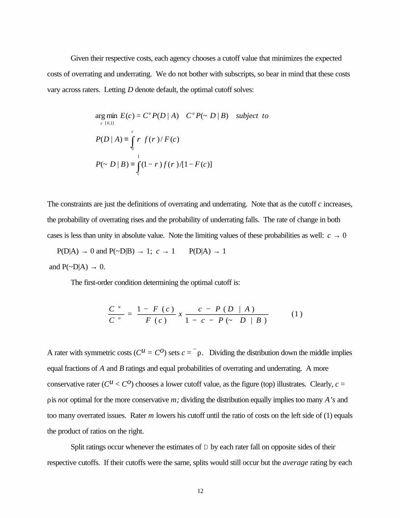
Given their respective costs, each agency chooses a cutoff value that minimizes the expected
costs of overrating and underrating. We do not bother with subscripts, so bear in mind that these costs
vary across raters. Letting D denote default, the optimal cutoff solves:
)](1/[)()1()|(~
)(/)()|(
)|(~)|()(minarg
1
0
]1,0[
cFfBDP
cFfADP
tosubjectBDPCADPCcE
c
c
uo
c
−−≡
≡
+=
∫
∫
∈
ρρ
ρρ
The constraints are just the definitions of overrating and underrating. Note that as the cutoff c increases,
the probability of overrating rises and the probability of underrating falls. The rate of change in both
cases is less than unity in absolute value. Note the limiting values of these probabilities as well: c → 0
⇒ P(D|A) → 0 and P(~D|B) → 1; c → 1 ⇒ P(D|A) → 1
and P(~D|A) → 0.
The first-order condition determining the optimal cutoff is:
)1()|(~1
)|()(
)(1BDPc
ADPcx
cFcF
CC
o
u
−−−−=
A rater with symmetric costs (Cu = Co) sets c = ρ. Dividing the distribution down the middle implies
equal fractions of A and B ratings and equal probabilities of overrating and underrating. A more
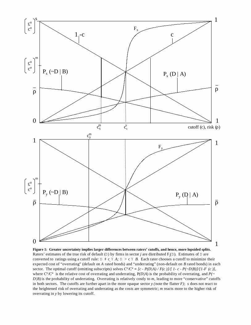
conservative rater (Cu < Co) chooses a lower cutoff value, as the figure (top) illustrates. Clearly, c =
ρis not optimal for the more conservative m; dividing the distribution equally implies too many A’s and
too many overrated issues. Rater m lowers his cutoff until the ratio of costs on the left side of (1) equals
the product of ratios on the right.
Split ratings occur whenever the estimates of D by each rater fall on opposite sides of their
respective cutoffs. If their cutoffs were the same, splits would still occur but the average rating by each
13
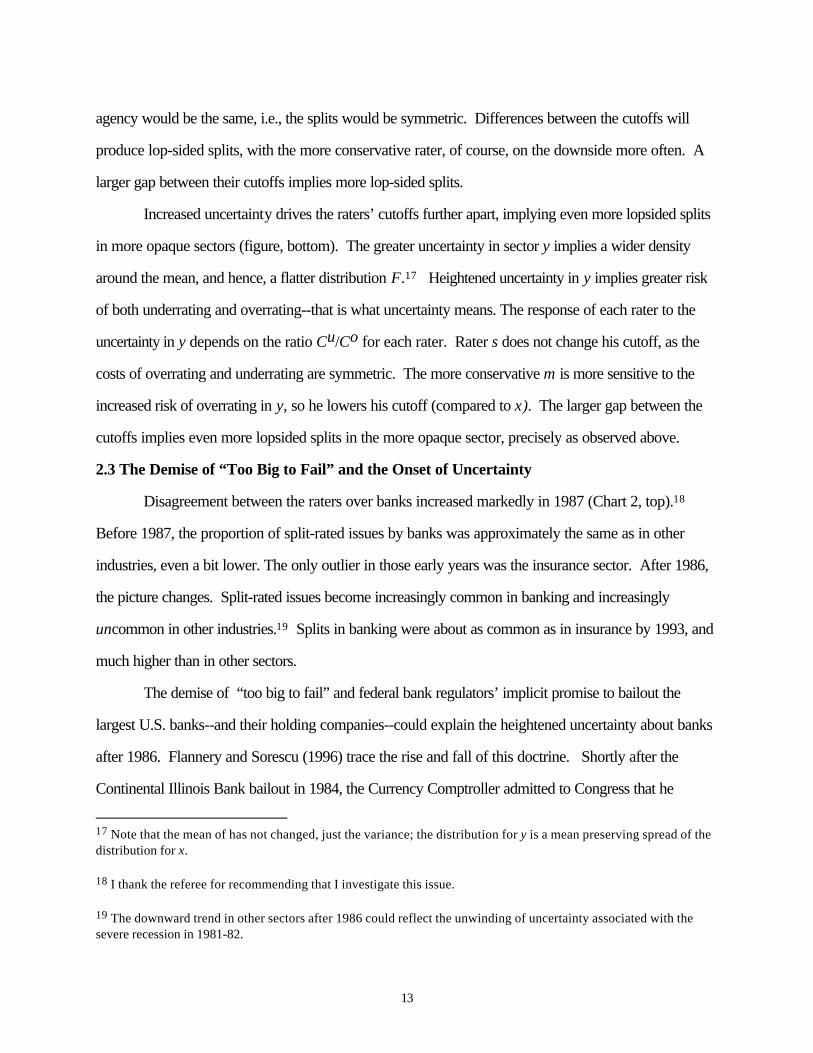
agency would be the same, i.e., the splits would be symmetric. Differences between the cutoffs will
produce lop-sided splits, with the more conservative rater, of course, on the downside more often. A
larger gap between their cutoffs implies more lop-sided splits.
Increased uncertainty drives the raters’ cutoffs further apart, implying even more lopsided splits
in more opaque sectors (figure, bottom). The greater uncertainty in sector y implies a wider density
around the mean, and hence, a flatter distribution F.17 Heightened uncertainty in y implies greater risk
of both underrating and overrating--that is what uncertainty means. The response of each rater to the
uncertainty in y depends on the ratio Cu/Co for each rater. Rater s does not change his cutoff, as the
costs of overrating and underrating are symmetric. The more conservative m is more sensitive to the
increased risk of overrating in y, so he lowers his cutoff (compared to x). The larger gap between the
cutoffs implies even more lopsided splits in the more opaque sector, precisely as observed above.
2.3 The Demise of “Too Big to Fail” and the Onset of Uncertainty
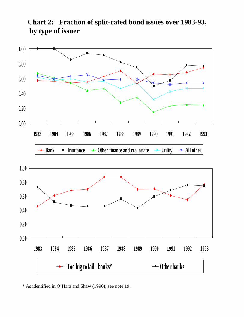
Disagreement between the raters over banks increased markedly in 1987 (Chart 2, top).18
Before 1987, the proportion of split-rated issues by banks was approximately the same as in other
industries, even a bit lower. The only outlier in those early years was the insurance sector. After 1986,
the picture changes. Split-rated issues become increasingly common in banking and increasingly
uncommon in other industries.19 Splits in banking were about as common as in insurance by 1993, and
much higher than in other sectors.
The demise of “too big to fail” and federal bank regulators’ implicit promise to bailout the
largest U.S. banks--and their holding companies--could explain the heightened uncertainty about banks
after 1986. Flannery and Sorescu (1996) trace the rise and fall of this doctrine. Shortly after the
Continental Illinois Bank bailout in 1984, the Currency Comptroller admitted to Congress that he
17 Note that the mean of has not changed, just the variance; the distribution for y is a mean preserving spread of thedistribution for x.
18 I thank the referee for recommending that I investigate this issue.
19 The downward trend in other sectors after 1986 could reflect the unwinding of uncertainty associated with thesevere recession in 1981-82.
14
considered the largest U.S. banks simply “too big to fail” (without unacceptably hazards to the financial
system). Stock returns of the lucky eleven banks actually named as such rose abnormally following this
remarkable announcement (O’Hara and Shaw 1990), suggesting the implicit guarantee to bank holding
company investors was valued in the market.20 The certainty associated with this guarantee also
explains the high rate of consensus between bond raters over this era. The demise of TBTF began
around 1986, when regulators devised ways to save the bank without sparing the holding company.21
As stocks and bonds are typically issued by the holding company, this innovation substantially
weakened the implicit government guarantee to holders of these claims. In fact, the relationship
between bank bond spreads and risk tightened considerably after 1986 (Flannery and Sorescu 1996),
suggesting that investors were trying to heed the risks of their bank holdings.22
Trying perhaps, but not necessarily succeeding; increased disagreement between bond raters
after 1986 suggests that evaluating bank risk was not trivial for the agencies. Disagreement between the
raters after 1986 was even more pronounced over the erstwhile TBTF banks (chart 2, lower),
suggesting that shift in regulatory policy did indeed contribute to raters’ uncertainty after 1986.
The obvious question here is whether it was the banks raters were unsure about, or the
regulators? The credibility of the policy shift away from TBTF was not unquestioned; raters may simply
had differing estimates about regulators’ resolve to actually permit a very large U.S. bank to fail.
Perhaps raters were disagreeing about the probability of a bailout, in other words, and not the
20 The comptroller did not actually name banks, but the Wall Street Journal did: Bank America, Bankers Trust, ChaseManhattan, Chemical Bank, Citicorp, Continental Illinois, First Chicago, JP Morgan, Manufacturers Hanover, SecurityPacific, Wells Fargo (O’Hara and Shaw 1990).
21 When First National Bank of Oklahoma City failed in July 1986, the FDIC underwrote a transaction whereby thepurchaser of the failing bank accepted the obligations of the bank only; the holding company of the bank defaultedon its notes and debentures. Many of the bank and thrift failures after that event involved losses to the bondholdersof the holding company.
22 Avery et al. (1988) documented the weak link between bank holding company bond spreads and risk during thevery early 1980s. Gorton and Santomero (1990) confirm their findings.

15
probability of default. To show that the uncertainty over banks was in fact the banks per se,
disagreement between the raters must be linked to the assets of the banks themselves.
3. The Opacity of Banks’ Assets
Drawing from the intermediation and agency literature, this section argues that the unique
nature of banks assets, combined with their high leverage, create fundamental uncertainty for investors
and analysts. Analysts are quoted throughout this section to reinforce the theory, but the real evidence
comes later.
3.1. What’s Different About Banks?
At the most basic level, it is the financial nature of their assets that distinguishes banks from other
firms. The heart of a bank is a vault with a lot of paper in it: loan documents, securities, and cash.
Compared to other firms, banks hold very few assets that are physically fixed--bolted to the floor--in
other words. The absence of fixed assets may invite asset substitution and other agency problems
between the banks’ owners and managers and its creditors. Financial assets generally may create
collateral uncertainty for bank investors.
The particular financial assets held by banks may invite agency problems as well. Primary
among their assets are loans to smaller, more opaque borrowers identified as the raison d etre for
banks (Diamond 1984). In theory, savers delegate this monitoring role to banks or other
intermediaries so that each and every saver need not monitor borrowers directly. This delegated
monitoring role may be efficient from a capital allocation perspective, but bank opacity may be an
inevitable consequence: Lending to opaque borrowers may cause opaque banks.23 Moody’s analysts
readily admit the difficulty of evaluating bank loan quality:
The assessment of a bank’s asset quality is both the most important and the most difficultelement of bank analysis. Perhaps the biggest risk in holding a bank security is that theinstitution as substantial unrecognized asset quality problems. . . As there can be noobjective standard in this area, the analyst must exercise his or her judgement using
23 Whether banks are better informed about the aggregate risk in their loan portfolio, however, depends on if banksfully diversify their loan portfolios. If banks are able to fully the diversify the idiosyncratic risk of their loans,outsiders only have to agree on the aggregate risk that banks are unable to shed. Krasa and Villamil (1992) present amodel in which limited diversification is optimal because of monitoring costs associated with diversified portfolios.
16
what can only be impressionistic information. The analyst cannot examine each loan.”(Moody’s Special Comment, 1993, p. 3, emphasis added)
Trading assets are another potential source of uncertainty for bank outsiders. Unlike bank loans,
trading assets are necessarily transparent, and hence, liquid. The trouble with trading is that positions
are slippery; traders can change positions so rapidly that outsiders cannot keep track. Myers and
Ragan (1997) call this the “paradox of liquidity;” liquidity enables trading and trading is hard to monitor.
Hentschel and Smith (1996) also stress the agency risks associated with trading, not just between
owners and creditors, but between traders and their principals: managers and shareholders.24 Traders
are motivated to take excessive risk because of the asymmetric incentives they typically face; they
share the upside, via bonuses, but downside liability is limited. Trading positions are relatively easy to
conceal, they further note, by the use of leverage (which minimizes the detectable impact on cash flow).
Analysts, Moody’s again,
admit the uncertainty surrounding trading activity: “. . . monitoring traders can be cumbersome . . .
(the) manager or auditor may be potentially at a lost about what is going on (Moody’s Special
Comment, 1992, p. 4).
Compounding the inherent uncertainty over these sorts of assets is the high leverage at banks.
Apart from the inherent risks associated with high leverage, it may also invite agency problems, as
shareholders are of leveraged firms are inclined to take more risk than creditors bargained for (Jensen
and Meckling 1976). Banks can effect this asset substitution by following riskier loan underwriting and
trading strategies. Analysts recognize the role of capital as a risk mitigating or signaling device:
Capital levels provide a readily accessible indication as to wheremanagement wishes to place the bank on the risk/return continuum...Banks with high capital levels tend to have good asset quality andconservative strategies, while those with low capital levels often areaggressive and risk-prone. This is not an infallible tool, but it is accurateoften enough to be useful (Moody’s Special Comment, 1993, p.5).
24 Catastrophic trading losses at banks highlight the agency risks of “rogue” traders. Baring, a venerable Britishbank, was bankrupted by a single trader. At Daiwa Bank, a senior bond trader managed to lose over $1 billion whilemaintaining secret accounts for eleven years (Hentschel and Smith 1996).
17
3.2. Disagreement over Bank Assets
To test whether banks’ assets generate uncertainty for raters, we now combine the ratings data
on bank holding companies (BHC) with detailed data on their assets. The asset data are from the
regulatory Call Report BHCs must file (form Y9C). Issues after 1986:2, when the Call Reports
became quarterly, were matched with balance sheet data from the quarter before issuance. Issues
before 1986:2 were matched with call report data from one or two quarters before issuance, whichever
was available. Complete data were available for 532 bonds issued by 96 different BHCs or their
subsidiaries.
The assets are summarized in Table 6. Loans and leases make up the bulk of banks’ assets,
followed by securities and cash and deposits. Trading assets comprise only a small share of total assets
on average, but the range of values is large; trading has become a big business indeed for roughly a
dozen, large “trading” banks.25 Taken together, these and the other financial assets account for over
90 percent of all bank assets on average. Fixed assets, by contrast, make up only about three percent
of assets. Banks’ have their premises and the real estate they collect on defaulted loans (“other real
estate”). Note the high leverage at banks as well; the capital-to-asset ratio averaged only 6.3 percent,
much lower than for non-banks as a whole.
To test how variation in the mix of banks’ assets affects uncertainty about its risk, we regress
the absolute difference between the ratings (0,1, 2 +) on these various asset shares.26
The regression included the average rating and other issue characteristics, as well as year dummies for
the years of issuance. Estimation was by ordered probit. The results are in Table 7.
25 Included in the trading account are “the assets held for resale by a bank holding company that regularly engagesin trading activities. Assets in trading accounts are to are generally held for a short period of time. Tradingaccounts...contain only instruments purchased with the intent to resell.” (Instructions for Federal Call Reports, formY9-C). Also included are gains and losses on derivative contracts--options, futures, etc. The notional amounts ofthese contracts are counted off-balance sheet. Securities to be held to maturity are counted in the securities line ofthe balance sheet.
26 The 18 differences of three notches and one difference of four were rounded to 2. Not rounding does not changethe results. Using SPLIT instead of the absolute difference produces very similar results.
18
Disagreement between raters is positively related to the average (numerical) rating on bank
issues, as was found for issues generally. Face value enters negatively, as before, but is only weakly
significant here. Maturity is insignificant. The year dummy coefficients confirm the marked increase in
disagreement after 1986 and the demise of “too big to fail.”
Of primary interest is how variation in the asset shares across banks affects disagreement
between the raters. The excluded asset is securities, which makes it the benchmark; the other asset
coefficients indicate how substitution into that asset out of securities affects the difference between
ratings. As a whole, the mix of assets does matter; a Chi-squared test easily rejects that the
coefficients are jointly zero. The total of assets matters as well, although the alternating signs on total
assets and its square suggest a quadratic (two-edged) relationship between bank size and uncertainty.27
The individual assets coefficients are consistent with theories just discussed. Loans and leases
enter negatively, implying more disagreement between raters as banks substitute loans for securities.
Trading also increases the likelihood of disagreement, as do increased holdings of cash and deposits.
Although not predicted, the latter result seems consistent with the results on trading; cash is by definition
the most liquid of assets, with all the attendant risks of agency problems.28
Banks’ more fixed assets tend to resolve uncertainty.29 Premises is negative and significant.
Other real estate also enters negatively, though the coefficient is insignificant. The opposite signs on
27 Size may be a two-edged sword for analysts; bigger banks may be better diversified, meaning less concern aboutthe idiosyncratic risks at each bank, but greater size also means analysts must consider managers’ ability to copewith more complex, less focused operations. See Demsetz and Strahan (1997) for evidence on bank size,diversification, and risk.
28 Jensen’s (1986) free cash-flow hypothesis provides another explanation: creditors (or analysts) may be nervouswhen the see excessive cash holding, since they cannot be sure how the managers will dispose of the cash. Thiscash result holds even if the banks with very high cash holdings are excluded. Simply accounting for cash can betricky, as Guthman (1953, p. 76) warns in his guide to financial analysts: “Cash on hand has been distorted by theinexpert and the unscrupulous to mean a variety of items. It has been stretched to include “IOU’s” to employeesloans to officers, advances to salesman, and similar noncash items. Cash-on-Hand...should be comparatively small; ifit is not, the possibility of some such error as is here indicated should be considered.”
29 While the coefficients are premises and other real estate arean order larger than on loans, recall that the mean andstandard deviations of the former are an order smaller. Note that other real estate also enters negatively, althoughthe coefficient is insignificant.
19
trading and premises have a nice symmetry, since on the spectrum of agency risks, these two assets
seem like the endpoints. The rub, of course, is that fixed assets are rare at banks as a whole.
Disagreement between the raters is also decreasing in the level of capital, also as expected.
The link here between capital and rater disagreement presumably reflects the role of capital role in
resolving uncertainty; the risk-reducing role of capital should be picked up with the average rating.30
3.2.1. Capital Mitigates Uncertainty
The potential for capital to resolve uncertainty implies an interaction between banks’ capital
positions and outsiders’ uncertainty about their risk. If capital mitigates the agency problems associated
with banks more opaque or slippery assets, the impact of increased lending and trading on rater
uncertainty should be less pronounced at more highly capitalized banks. To investigate, the sample of
bank issues was divided at the median capital-to-asset ratio of the issuers and regression above was
estimated separately for the low-capital and high-capital issuers.
The results in Table 8 largely support the hypothesis. Loans and leases cause disagreement
between bond raters only if the bonds are issued by relatively poorly capitalized banks. Likewise with
trading; trading assets are more likely to cause bonds split only at the banks with below median capital
ratios. The effects of premises are very similar across high capital and low capital banks, but increases
in the banks’ other fixed asset (other real estate) reduces the disagreement only the poorly capitalized
banks. The effect of changes in overall asset size also depends on capitalization; assets enter
significantly for the low-capital banks, but not the high-capital banks. The coefficients on the bond
characteristics were not significantly different across the two sets of banks. The equivalence of the year
dummy coefficients across the two sets cannot be rejected (except for 1985), but the increased
disagreement after 1986 appears somewhat more pronounced at the low-capital banks.
3.2.2. Fixed effects
30 The average numerical rating is in fact strongly, negatively correlated with bank capital.
20
A regression with a fixed effect for each issuer is estimated as a final robustness check. Adding
a fixed effect tells us if whether is variation in the mix of assets across or within banks behind the results
in Table 7. Trading assets, for example, are concentrated among a dozen or so “trading” banks so
there is a question of whether it is trading per se that confuses the raters, or whether trading simply
signals some other difference about these banks. Adding fixed effects to an ordered probit equation is
not trivial, however, so instead we report OLS estimates with and without a fixed effect (Table 9).
Adding a fixed effect leaves most of the results unchanged. Substitutions of loans and leases for
securities with a bank increases disagreement between raters, as do substitutions of cash and trading
assets for securities. Increased capital within a bank reduces disagreements, with or without the fixed
effect, but the within estimates (with the fixed estimates) are more significant.
Adding the fixed effect reverses the sign on premises, however. Variation in premises between
banks, in other words, tends to reduce disagreement between the raters. That result is consistent with
the earlier, probit estimates. Increased premises within a bank, however, tends to increase
disagreement, perhaps because of the uncertainty associated with bank (via acquisitions of banks with
branch networks). In any case, variation across banks seems like the relevant experiment here, and
those results square with the idea that fixed assets tend to reduce the uncertainty associated with asset
substitution. Note that other real estate—the other fixed asset at banks--is significantly negative with
the fixed effect included.
4. Conclusion
Disagreement between bond raters makes a good proxy for the uncertainty associated with
asymmetric information and other such frictions.31 Splits between Moody’s and S&P increase with
average of the two ratings, as one would expect if risk and uncertainty are positively related.
Disagreement between raters also increases with maturity (given risk), but decreases with the size of the
issue, presumably because the smaller issues are by smaller, more opaque firms.
31 Bonaccorsi di Patti and Dell’ Aricia (2000) use split bond ratings to investigate how information asymmetriesbetween bank and borrower affect the birth of new firms in Italy.
21
The pattern of disagreement across sectors suggests a continuum of opacity, with the more
asset-backed sectors or securities at the transparent end and the financial intermediaries--banks and
insurers--at the other. Utilities and the assets backed bonds favored by finance companies generated
relatively little disagreement between raters, suggesting the risk of these industries (or securities) are
relatively easy to quantify. The raters were much more likely to differ over insurance and banking
firms’ bonds. The splits over the intermediaries was also more lop-sided, the predicted by the model of
ratings under uncertainty developed here. The timing was right as well; splits over banks increased
markedly after 1986, consistent with Flannery and Sorescus’ (1990) thesis that the demise of “too big
to fail,” after that date forced investors and raters to heed the risk of banks more closely.
In any given year, the disagreement over banks can be traced to their assets, suggesting the veil
is to some extent inherent to the business. Loans--the defining asset of a bank--are a significant source
of disagreement between raters, as are the trading assets that are prominent on the books of the dozen
or so large, trading banks. Trading assets are not necessarily opaque and illiquid, like loans, they are
extremely liquid and “slippery;” trading positions can change instantaneously, which makes them hard to
monitor from outside the bank. Cash also creates splits between the raters, while premises or banks’
other fixed assets tend to reduce disagreement; the vault, in other words, matters more than the cash it
contains, presumably because cash can disappear but the vault is hard to move. Short of nailing down
more of their assets, some degree of uncertainty over banks seems inevitable.
The relative opacity of banks provides some justification for government intervention in the
banking market, since runs, contagion, and other strains of systemic risk stem ultimately from the opacity
of banks’ assets. Saying that does not imply necessarily imply that the current regulatory structure is
optimal, of course. The push for increased market discipline and disclosure may shed light. But
reformers should remember what they are dealing with. To use a popular metaphor: banks may be the
black holes of the financial universe; hugely powerful and influential, but to some irreducible extent--
unfathomable.
22
ReferencesBerger, A., 1991, “Market Discipline in Banking,” Proceedings of a conference on Bank
Structure and Competition, Federal Reserve Bank of Chicago.
_______A. Kashyap, and J. Scalise, 1995, “The Transformation of the U.S. Banking Industry: What a Long, Strange Trip It’s Been,” Brookings Papers on Economic Activity, 2, 55-218.
Bomberger, W., 1996, “Disagreement as a Measure of Uncertainty,” Journal of Money, Credit, and Banking, 28, # 381-392.
E. Bonaccorsi di Patti and G. Dell’ Ariccia, “Bank Competition and Firm Creation,” mimeo,Bank of Italy and International Monetary Fund.
Cantor R. and F. Packer, 1994, “The Credit Rating Industry,” Federal Reserve Bank of New York Quarterly Review, 12, 1-26.
______, 1996, “Multiple Ratings and Credit Standards: Differences of Opinion in the Credit RatingIndustry,” Federal Reserve Bank of New York Staff Report, 12.
______ and K. Cole, 1997, “Split Ratings and the Pricing of Credit Risk, Federal Reserve Bank of New York Research Paper, # 9711.
Carey, M., S. Prowse, J. Rea, and G. Udell, 1993, “Recent Developments in the Market for Privately Placed Debt,” Federal Reserve Bulletin, January, p. 77-93.
Crabbe, L. 1996, Fixed Income Weekly, January 26.
Demsetz, Rebecca S. and Philip E. Strahan, 1997 “Diversification, Size, and Risk at Bank HoldingCompanies,” Journal of Money, Credit, and Banking 29.
Dewatripont, M. and J. Tirole, 1993, The Prudential Regulation of Banks, MIT Press, Cambridge.
Diamond, D, 1984, “Financial Intermediation and Delegated Monitoring,” Review of Economic Studies, 51, 393-414.
Ederington, Louis, 1986, “Why Split Ratings Occur,” Financial Management, Spring, p. 37-47.
Flannery, M, 1994, “Debt Maturity and the Deadweight Cost of Leverage: Optimally Financing Banking Firms” American Economic Review, 84, 320-331.
23
_______, Kwan, S. and M. Nimalendran, 1998, “Market Evidence on the Opaqueness of Banking Firms’ Assets.” Mimeo, University of Florida.
_______ and S. Sorescu, 1996, “Evidence of Bank Market Discipline in Subordinated Debenture Yields: 1983-91.” Journal of Finance, LI, 4, September, 1347-1377.
________, 1998. “Using Market Information in Bank Supervision: A Review of the U.S. Empirical Evidence.” Journal of Money, Credit, and Banking, 30, August, 273-305.
Guthman, Harry, G., 1953, Analysis of Financial Statements, Prentice-Hall, New York, fourth edition.
T. Hannan and G. Hanweck, 1988, “Bank Insolvency Risk and the Market for Large Certificates of Deposit.” 20, May, 203-211.
Hentschel, L. and C. Smith, 1996, “Derivatives Regulation: Implications for Central Banks,”Monetary Policy and Financial Markets, Studienzentrum Gerzensee, October.
Krasa, S and Anne P. Villamil, 1992 “A Theory of Optimal Bank Size,” Oxford EconomicPapers, 44: 752-749.
Jayaratne, J. and D. Morgan, 2000, “Capital Market Imperfections and Deposit Constraints on Banks, Journal of Money, Credit, and Banking, February.
Jensen, M., 1986, “Agency Costs of Free Cash Flow, Corporate Finance, and Takeovers,”American Economic Review, 76, 323-29.
Jensen, M.C. and W. Meckling, 1976, “Theory of the Firm: Managerial Behavior, Agency Costs, and Ownership Structure,” Journal of Financial Economics 3, 305-360.
Knight, Frank H., 1921, Risk, Uncertainty, and Profit, Houghton Mifflin Company, New York,
Mahoney, Christopher, 1993, “Bank Credit Analysis: Historical Origins and Current Practice.” Moody’s Special Comment, Moody’s Investors Service, New York, June.
Moody’s Special Comment, 1991,“Securities Derivatives: Risks and Opportunities,” January 16.
Moody’s Special Comment, 1993, “Moody’s Approach to the Credit Analysis of Banks and Bank Holding Companies,” April.
Morgan, Donald P. and K. Stiroh, 1999, “Bond Market Discipline of Banks: Is the Market Tough Enough on Banks,” Federal Reserve Bank of New York Staff Study # 95.
24
Myers, S. and R. Rajan, 1998, “The Paradox of Liquidity,” Quarterly Journal of Economics, CXIII, August, 733-773.
O’Hara, M., and W. Shaw, 1990, “Deposit Insurance and Wealth Effects,” Journal of Finance,45, 1587-1600.
Reiss, Peter, 1989, “Economic and Financial Determinants of Oil and Gas Exploration Activity,”National Bureau of Economic Research Working Paper 3077, Cambridge, MA.
Stata Reference Manual, 1999, release 6, various volumes, Stata Press, College Station, Texas.
Seiberg, J, 1996, “Fed Sets capital Standard for Major Trading Banks,” American Banker, p.1.
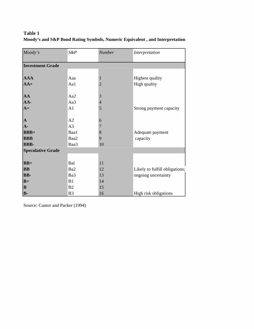
Table 1Moody’s and S&P Bond Rating Symbols, Numeric Equivalent , and Interpretation
Moody’s S&P Number Interpretation
Investment Grade
AAA Aaa 1 Highest qualityAA+ Aa1 2 High quality
AA Aa2 3AA- Aa3 4A+ A1 5 Strong payment capacity
A A2 6A- A3 7BBB+ Baa1 8 Adequate paymentBBB Baa2 9 capacityBBB- Baa3 10Speculative Grade
BB+ Bal 11BB Ba2 12 Likely to fulfill obligations;BB- Ba3 13 ongoing uncertaintyB+ B1 14B B2 15B- B3 16 High risk obligations
Source: Cantor and Packer (1994)
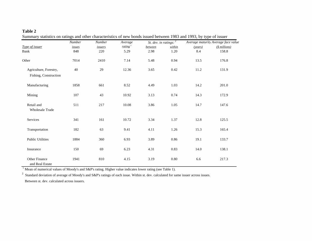
Table 2Summary statistics on ratings and other characteristics of new bonds issued between 1983 and 1993, by type of issuer
Number Number Average Average maturity Average face valueType of issuer issues issuers rating 2
between within (years) ($ millions)Bank 848 220 5.29 2.98 1.20 8.4 158.8
Other 7014 2410 7.14 5.48 0.94 13.5 176.8
Agriculture, Forestry, 40 29 12.36 3.65 0.42 11.2 131.9
Fishing, Construction
Manufacturing 1858 661 8.52 4.49 1.03 14.2 201.0
Mining 107 43 10.92 3.13 0.74 14.3 172.9
Retail and 511 217 10.08 3.86 1.05 14.7 147.6 Wholesale Trade
Services 341 161 10.72 3.34 1.37 12.8 125.5
Transportation 182 63 9.41 4.11 1.26 15.3 165.4
Public Utilities 1884 360 6.93 3.89 0.86 19.1 133.7
Insurance 150 69 6.23 4.31 0.83 14.0 138.1
Other Finance 1941 810 4.15 3.19 0.80 6.6 217.3 and Real Estate
1 Mean of numerical values of Moody's and S&P's rating. Higher value indicates lower rating (see Table 1). 2 Standard deviation of average of Moody's and S&P's ratings of each issue. Within st. dev. calculated for same issuer across issues.
Between st. dev. calculated across issuers.
St. dev. in ratings: 2
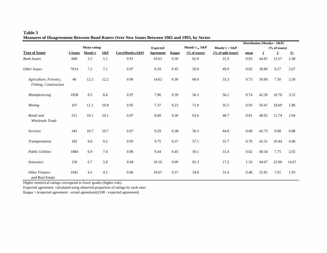
Table 3Measures of Disagreement Between Bond Raters Over New Issues Between 1983 and 1993, by Sector
Distribution |Moodys - S&P|: Mean rating: Expected Moody's ≠ ≠ S&P Moody's < S&P (% of issues)
Type of Issuer # Issues Moody's S&P Corr(Moodys,S&P) Agreement Kappa (% of issues) (% of split issues) mean 1 2 3+
Bank Issues 848 5.5 5.1 0.91 10.63 0.30 62.9 31.9 0.83 44.81 15.57 2.48
Other Issues 7014 7.2 7.1 0.97 8.29 0.45 50.0 49.9 0.65 38.80 9.27 2.67
Agriculture, Forestry, 40 12.5 12.2 0.96 14.62 0.30 60.0 33.3 0.73 50.00 7.50 2.50 Fishing, Construction
Manufacturing 1858 8.5 8.6 0.97 7.96 0.39 56.3 56.2 0.74 42.30 10.76 3.22
Mining 107 11.1 10.8 0.95 7.37 0.23 71.0 35.5 0.93 50.47 18.69 1.86
Retail and 511 10.1 10.1 0.97 8.68 0.30 63.6 48.7 0.81 48.92 11.74 2.94 Wholesale Trade
Services 341 10.7 10.7 0.97 9.29 0.38 56.3 44.8 0.68 45.75 9.68 0.88
Transportation 182 9.6 9.2 0.95 9.75 0.37 57.1 31.7 0.76 42.31 10.44 4.40
Public Utilities 1884 6.9 7.0 0.96 9.44 0.45 50.1 31.4 0.62 40.34 7.75 2.02
Insurance 150 6.7 5.8 0.94 10.16 0.09 81.3 17.2 1.33 44.67 22.00 14.67
Other Finance 1941 4.2 4.1 0.96 18.67 0.57 34.8 31.4 0.46 25.81 7.01 1.95 and Real Estate
Higher numerical ratings correspond to lower grades (higher risk). Expected agreement calculated using observed proportion of ratings by each rater. Kappa = (expected agreement - actual agreement)/(100 - expected agreement)
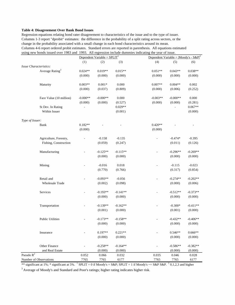
Table 4: Disagreement Over Bank Bond IssuesRegression equations relating bond rater disagreement to characteristics of the issue and to the type of issuer. Columns 1-3 report "dprobit" estimates: the difference in the probability of a split rating across sectors, or the change in the probability associated with a small change in each bond characteristics around its mean. Columns 4-6 report ordered probit estimates. Standard errors are reported in parenthesis. All equations estimatedusing new bonds issued over 1983 and 1993. All regression include dummies indicating the year of issue.
Dependent Variable = SPLIT1 Dependent Variable = |Moody's - S&P|2
(1) (2) (3) (4) (5) (6)Issue Characteristics:
Average Rating3 0.024** 0.019** 0.015** 0.051** 0.043** 0.038**(0.000) (0.000) (0.000) (0.000) (0.000) (0.000)
Maturity 0.003** 0.001* 0.000 0.007** 0.004** 0.002(0.000) (0.037) (0.809) (0.000) (0.006) (0.252)
Face Value (10 million) -0.000** -0.000** 0.000 -0.003** -0.000** 0.000(0.000) (0.000) (0.527) (0.000) (0.000) (0.281)
St Dev. In Rating - 0.029** - 0.067** Within Issuer (0.001) (0.000)
Type of Issuer:Bank 0.182** - - 0.420** - -
(0.000) (0.000)
Agriculture, Forestry, - -0.158 -0.135 - -0.474* -0.395 Fishing, Construction (0.059) (0.247) (0.011) (0.126)
Manufacturing - -0.125** -0.115** - -0.296** -0.269**(0.000) (0.000) (0.000) (0.000)
Mining - -0.016 0.018 - -0.115 -0.023(0.770) (0.766) (0.317) (0.854)
Retail and - -0.093** -0.056 - -0.274** -0.202** Wholesale Trade (0.002) (0.098) (0.000) (0.006)
Services - -0.193** -0.141** - -0.512** -0.373**(0.000) (0.000) (0.000) (0.000)
Transportation - -0.139** -0.162** - -0.300* -0.411**(0.001) (0.000) (0.001) (0.000)
Public Utilities - -0.173** -0.158** - -0.432** -0.406**(0.000) (0.000) (0.000) (0.000)
Insurance - 0.197** 0.221** - 0.546** 0.666**(0.000) (0.000) (0.000) (0.000)
Other Finance - -0.258** -0.164** - -0.586** -0.382** and Real Estate (0.000) (0.000) (0.000) (0.000)
Pseudo R2 0.052 0.066 0.032 0.035 0.046 0.028Number of Observations 7765 7765 6177 7765 7765 6177
** significant at 1%; * significant at 5%. 1 SPLIT = 0 if Moody's = S&P; SPLIT = 1 if Moody's ~= S&P S&P. 2 0,1,2,3 and higher3 Average of Moody's and Standard and Poor's ratings; higher rating indicates higher risk.
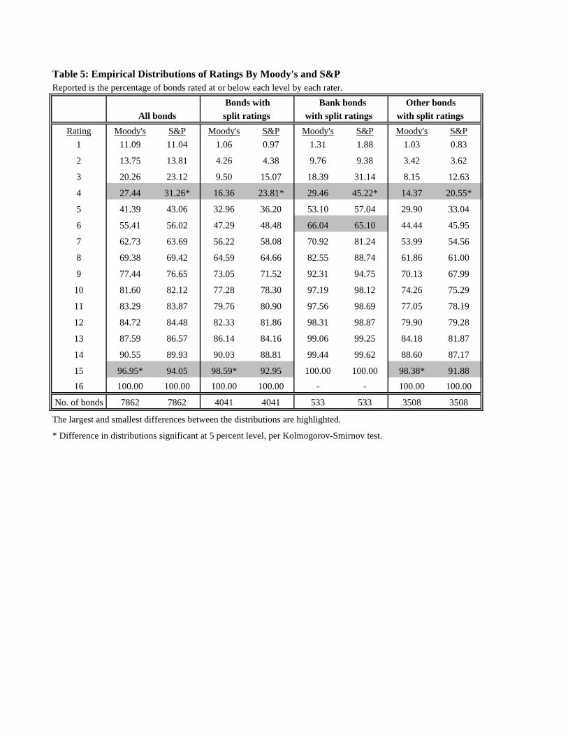
Table 5: Empirical Distributions of Ratings By Moody's and S&PReported is the percentage of bonds rated at or below each level by each rater.
Bonds with Bank bonds Other bonds All bonds split ratings with split ratings with split ratings
Rating Moody's S&P Moody's S&P Moody's S&P Moody's S&P1 11.09 11.04 1.06 0.97 1.31 1.88 1.03 0.83
2 13.75 13.81 4.26 4.38 9.76 9.38 3.42 3.62
3 20.26 23.12 9.50 15.07 18.39 31.14 8.15 12.63
4 27.44 31.26* 16.36 23.81* 29.46 45.22* 14.37 20.55*
5 41.39 43.06 32.96 36.20 53.10 57.04 29.90 33.04
6 55.41 56.02 47.29 48.48 66.04 65.10 44.44 45.95
7 62.73 63.69 56.22 58.08 70.92 81.24 53.99 54.56
8 69.38 69.42 64.59 64.66 82.55 88.74 61.86 61.00
9 77.44 76.65 73.05 71.52 92.31 94.75 70.13 67.99
10 81.60 82.12 77.28 78.30 97.19 98.12 74.26 75.29
11 83.29 83.87 79.76 80.90 97.56 98.69 77.05 78.19
12 84.72 84.48 82.33 81.86 98.31 98.87 79.90 79.28
13 87.59 86.57 86.14 84.16 99.06 99.25 84.18 81.87
14 90.55 89.93 90.03 88.81 99.44 99.62 88.60 87.17
15 96.95* 94.05 98.59* 92.95 100.00 100.00 98.38* 91.88
16 100.00 100.00 100.00 100.00 - - 100.00 100.00
No. of bonds 7862 7862 4041 4041 533 533 3508 3508
The largest and smallest differences between the distributions are highlighted.
* Difference in distributions significant at 5 percent level, per Kolmogorov-Smirnov test.
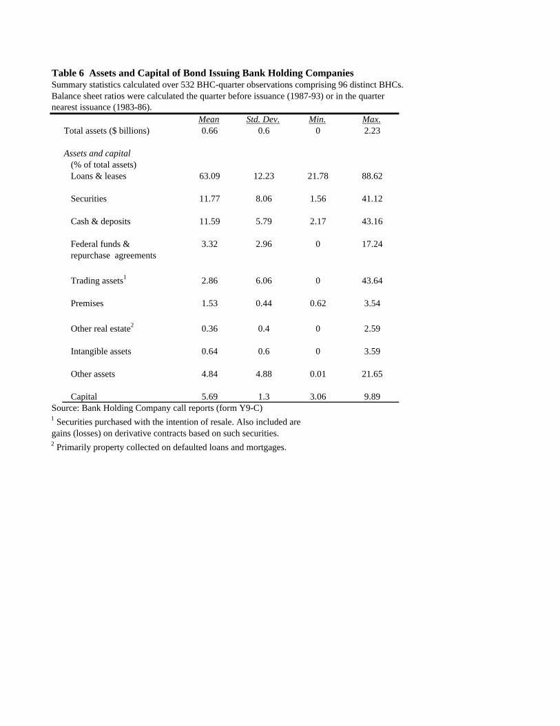
Table 6 Assets and Capital of Bond Issuing Bank Holding CompaniesSummary statistics calculated over 532 BHC-quarter observations comprising 96 distinct BHCs.Balance sheet ratios were calculated the quarter before issuance (1987-93) or in the quarternearest issuance (1983-86).
Mean Std. Dev. Min. Max.Total assets ($ billions) 0.66 0.6 0 2.23
Assets and capital (% of total assets) Loans & leases 63.09 12.23 21.78 88.62
Securities 11.77 8.06 1.56 41.12
Cash & deposits 11.59 5.79 2.17 43.16
Federal funds & 3.32 2.96 0 17.24 repurchase agreements
Trading assets1 2.86 6.06 0 43.64
Premises 1.53 0.44 0.62 3.54
Other real estate2 0.36 0.4 0 2.59
Intangible assets 0.64 0.6 0 3.59
Other assets 4.84 4.88 0.01 21.65
Capital 5.69 1.3 3.06 9.89Source: Bank Holding Company call reports (form Y9-C)1 Securities purchased with the intention of resale. Also included are gains (losses) on derivative contracts based on such securities. 2 Primarily property collected on defaulted loans and mortgages.
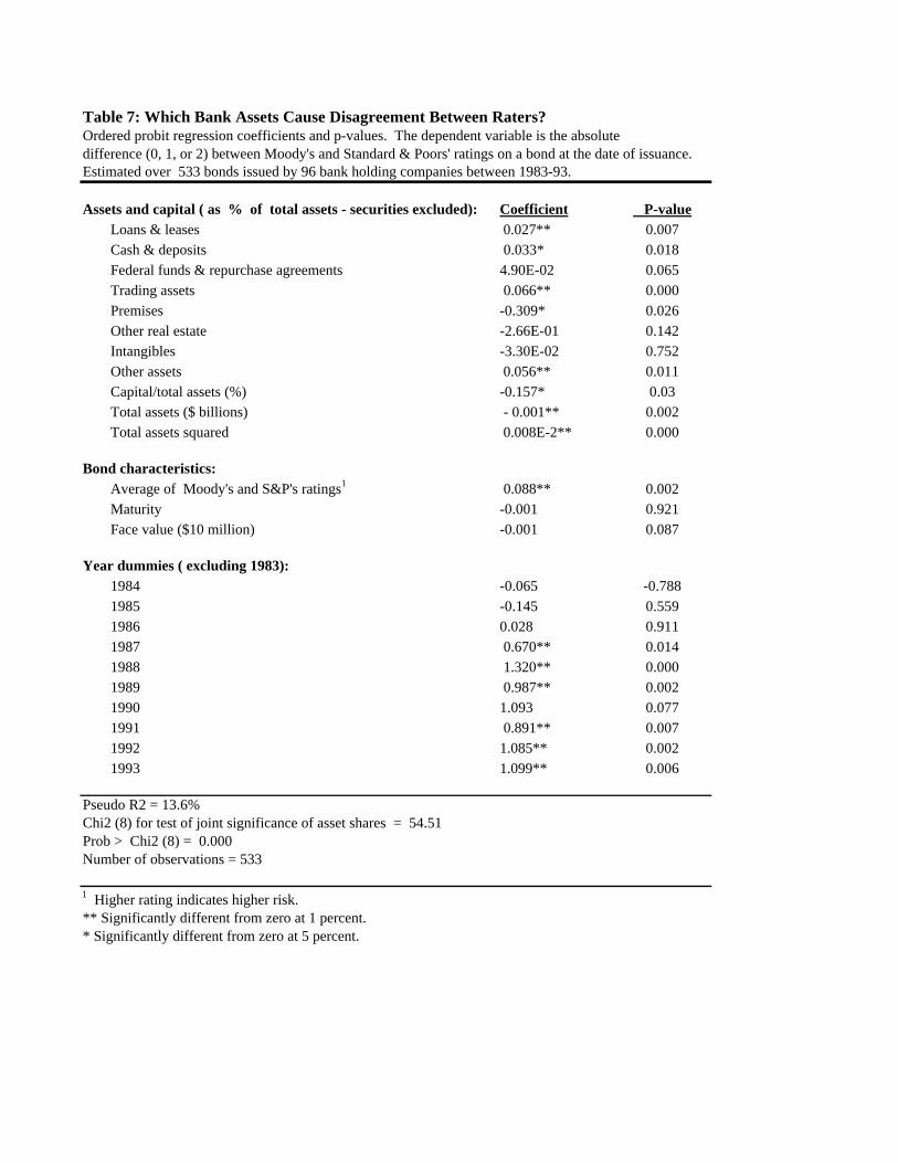
Table 7: Which Bank Assets Cause Disagreement Between Raters? Ordered probit regression coefficients and p-values. The dependent variable is the absolute difference (0, 1, or 2) between Moody's and Standard & Poors' ratings on a bond at the date of issuance. Estimated over 533 bonds issued by 96 bank holding companies between 1983-93.
Assets and capital ( as % of total assets - securities excluded): Coefficient P-valueLoans & leases 0.027** 0.007Cash & deposits 0.033* 0.018 Federal funds & repurchase agreements 4.90E-02 0.065Trading assets 0.066** 0.000Premises -0.309* 0.026Other real estate -2.66E-01 0.142Intangibles -3.30E-02 0.752Other assets 0.056** 0.011Capital/total assets (%) -0.157* 0.03Total assets ($ billions) - 0.001** 0.002Total assets squared 0.008E-2** 0.000
Bond characteristics: Average of Moody's and S&P's ratings1 0.088** 0.002Maturity -0.001 0.921Face value ($10 million) -0.001 0.087
Year dummies ( excluding 1983):1984 -0.065 -0.7881985 -0.145 0.5591986 0.028 0.9111987 0.670** 0.0141988 1.320** 0.0001989 0.987** 0.0021990 1.093 0.0771991 0.891** 0.0071992 1.085** 0.0021993 1.099** 0.006
Pseudo R2 = 13.6%Chi2 (8) for test of joint significance of asset shares = 54.51Prob > Chi2 (8) = 0.000Number of observations = 533
1 Higher rating indicates higher risk. ** Significantly different from zero at 1 percent.* Significantly different from zero at 5 percent.
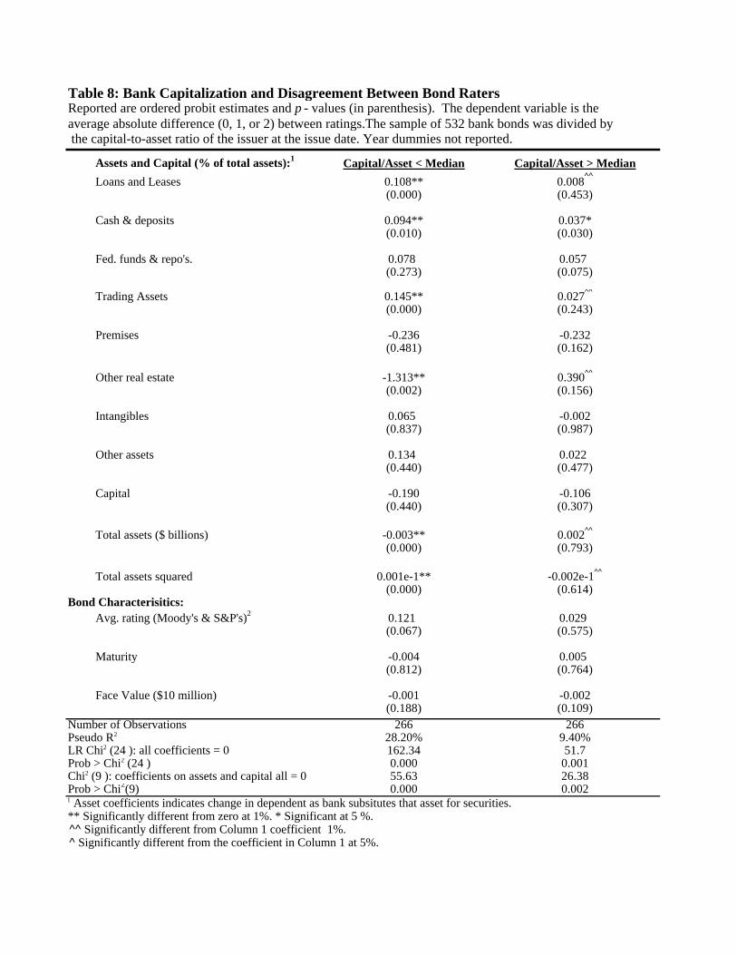
Table 8: Bank Capitalization and Disagreement Between Bond RatersReported are ordered probit estimates and p - values (in parenthesis). The dependent variable is the average absolute difference (0, 1, or 2) between ratings.The sample of 532 bank bonds was divided by the capital-to-asset ratio of the issuer at the issue date. Year dummies not reported.
Assets and Capital (% of total assets):1 Capital/Asset < Median Capital/Asset > Median
Loans and Leases 0.108** 0.008^^
(0.000) (0.453)
Cash & deposits 0.094** 0.037*(0.010) (0.030)
Fed. funds & repo's. 0.078 0.057(0.273) (0.075)
Trading Assets 0.145** 0.027^^
(0.000) (0.243)
Premises -0.236 -0.232(0.481) (0.162)
Other real estate -1.313** 0.390^^
(0.002) (0.156)
Intangibles 0.065 -0.002(0.837) (0.987)
Other assets 0.134 0.022(0.440) (0.477)
Capital -0.190 -0.106(0.440) (0.307)
Total assets ($ billions) -0.003** 0.002^^
(0.000) (0.793)
Total assets squared 0.001e-1** -0.002e-1^^
(0.000) (0.614)Bond Characterisitics:
Avg. rating (Moody's & S&P's)2 0.121 0.029(0.067) (0.575)
Maturity -0.004 0.005(0.812) (0.764)
Face Value ($10 million) -0.001 -0.002(0.188) (0.109)
Number of Observations 266 266Pseudo R2 28.20% 9.40%LR Chi2 (24 ): all coefficients = 0 162.34 51.7Prob > Chi2 (24 ) 0.000 0.001Chi2 (9 ): coefficients on assets and capital all = 0 55.63 26.38Prob > Chi2(9) 0.000 0.0021 Asset coefficients indicates change in dependent as bank subsitutes that asset for securities.** Significantly different from zero at 1%. * Significant at 5 %. ^^ Significantly different from Column 1 coefficient 1%. ^ Significantly different from the coefficient in Column 1 at 5%.
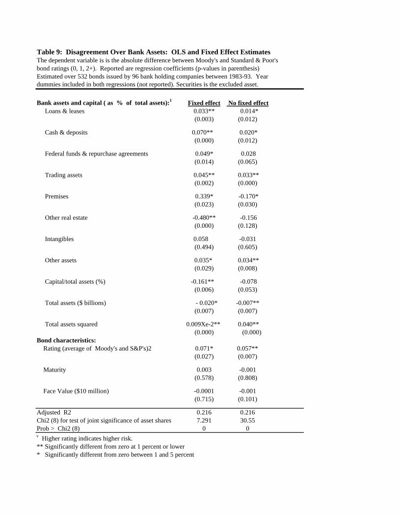
Table 9: Disagreement Over Bank Assets: OLS and Fixed Effect EstimatesThe dependent variable is is the absolute difference between Moody's and Standard & Poor's bond ratings (0, 1, 2+). Reported are regression coefficients (p-values in parenthesis)Estimated over 532 bonds issued by 96 bank holding companies between 1983-93. Year dummies included in both regressions (not reported). Securities is the excluded asset.
Bank assets and capital ( as % of total assets):1 Fixed effect No fixed effect Loans & leases 0.033** 0.014*
(0.003) (0.012)
Cash & deposits 0.070** 0.020*(0.000) (0.012)
Federal funds & repurchase agreements 0.049* 0.028(0.014) (0.065)
Trading assets 0.045** 0.033**(0.002) (0.000)
Premises 0.339* -0.170*(0.023) (0.030)
Other real estate -0.480** -0.156(0.000) (0.128)
Intangibles 0.058 -0.031 (0.494) (0.605)
Other assets 0.035* 0.034**(0.029) (0.008)
Capital/total assets (%) -0.161** -0.078 (0.006) (0.053)
Total assets ($ billions) - 0.020* -0.007**(0.007) (0.007)
Total assets squared 0.009Xe-2** 0.040**(0.000) (0.000)
Bond characteristics: Rating (average of Moody's and S&P's)2 0.071* 0.057** (0.027) (0.007)
Maturity 0.003 -0.001(0.578) (0.808)
Face Value ($10 million) -0.0001 -0.001(0.715) (0.101)
Adjusted R2 0.216 0.216Chi2 (8) for test of joint significance of asset shares 7.291 30.55Prob > Chi2 (8) 0 0v Higher rating indicates higher risk. ** Significantly different from zero at 1 percent or lower* Significantly different from zero between 1 and 5 percent
1 -c c
cx
Px (~D | B) Px (D | A)
0
1
1
0
1 1
1Figure 1: Greater uncertainty implies larger differences between raters’ cutoffs, and hence, more lopsided splits.Raters’ estimates of the true risk of default (D) by firms in sector j are distributed F j(D). Estimates of D areconverted to ratings using a cutoff rule: D # c, Y A; D > c Y B. Each rater chooses a cutoff to minimize theirexpected cost of “overrating” (default on A rated bonds) and “underrating” (non-default on B rated bonds) in eachsector. The optimal cutoff (omitting subscripts) solves Co/Cu = [c - P(D|A) / F(c )]/[ 1- c - P(~D|B)]/[1-F (c
)],where Co/Cu is the relative cost of overrating and underrating, P(D|A) is the probability of overrating, and P(~D|B) is the probability of underrating. Overrating is relatively costly to m, leading to more “conservative” cutoffsin both sectors. The cutoffs are further apart in the more opaque sector y (note the flatter F); s does not react tothe heightened risk of overrating and underrating as the costs are symmetric; m reacts more to the higher risk ofoverrating in y by lowering its cutoff.
ρ ρ
cxm
cym
Py (~D | B) Py (D | A)ρ ρ
s cutoff (c), risk (ρ)
Fx
cu
co
s
Fy
cu
co
m
cu
co
m
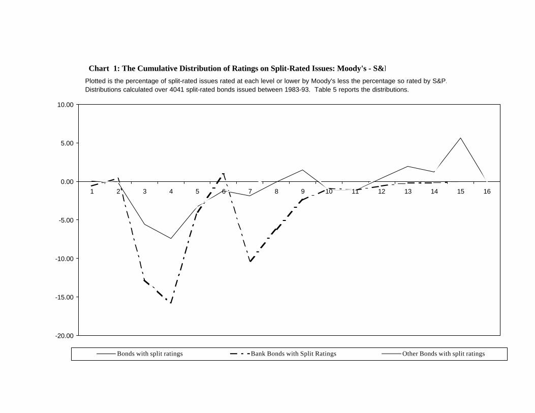
Chart 1: The Cumulative Distribution of Ratings on Split-Rated Issues: Moody's - S&P
-20.00
-15.00
-10.00
-5.00
0.00
5.00
10.00
1 2 3 4 5 6 7 8 9 10 11 12 13 14 15 16
Bonds with split ratings Bank Bonds with Split Ratings Other Bonds with split ratings
Plotted is the percentage of split-rated issues rated at each level or lower by Moody's less the percentage so rated by S&P. Distributions calculated over 4041 split-rated bonds issued between 1983-93. Table 5 reports the distributions.
0.00
0.20
0.40
0.60
0.80
1.00
1983 1984 1985 1986 1987 1988 1989 1990 1991 1992 1993
Bank Insurance Other finance and real estate Utility All other
0.00
0.20
0.40
0.60
0.80
1.00
1983 1984 1985 1986 1987 1988 1989 1990 1991 1992 1993
"Too big to fail" banks* Other banks
Chart 2: Fraction of split-rated bond issues over 1983-93, by type of issuer
* As identified in O’Hara and Shaw (1990); see note 19.


