No. DP17-2
RCESR Discussion Paper Series
Effects of the Entry and Exit of Products on Price Indexes
March 2017
Naohito Abe, Hitotsubashi University
Noriko Inakura, Osaka Sangyo University
Akiyuki Tonogi, Hitotsubashi University
The Research Center for Economic and Social Risks
Institute of Economic Research Hitotsubashi University
2-1 Naka, Kunitachi, Tokyo, 186-8603 JAPAN
http://risk.ier.hit-u.ac.jp/
RCESR
1
Effects of the Entry and Exit of Products on Price Indexes
Naohito Abe, Noriko Inakura, and Akiyuki Tonogi*
Abstract
This study analyzes the effects of product turnover for price measurements. In addition to variety
effects, we consider the effects of the price differentials between new and incumbent products.
The decomposition of a unit value price index (UVPI) into price change effects, substitution
effects, and turnover/new product effects reveals the magnitude and sources of differences
between the UVPI and the Cost of Living Indexes with variety effects. Using a large-scale
scanner data, we find that the product turnover effects that reflect the price gap between new and
old goods are quantitatively important when constructing a general price level index.
JEL Classification: C43, D12, E31
Keywords: Price Index, Cost of Living Index, Unit Value Price, POS Data
* Abe (corresponding author): Hitotsubashi University, Naka, Kunitachi, Tokyo 186-8603,
JAPAN. (E-mail: [email protected]). Inakura: Osaka Sangyo University, Nakagaito, Daito,
Osaka 574-8530, JAPAN. (Email: [email protected]). Tonogi: Hitotsubashi University,
Naka, Kunitachi, Tokyo 186-8603, JAPAN. (E-mail: [email protected]).
This paper is the product of a joint research project of the Institute of Economic Research,
Hitotsubashi University, the New Supermarket Association of Japan, and INTAGE Inc. We
are grateful for comments from Paul Schreyer at the Hitotsubashi-RIETI International
Workshop on Real Estate Market, Productivity, and Prices in 2016. We are also thankful for
comments from Yuko Ueno and seminar participants at the Bank of Japan and the University
of Tokyo. In addition, we would like to thank session participants at the European Economic
Association’s Congress in 2015 and the Japanese Economic Association’s Spring Meeting of
2015. This work was supported by JSPS Grant-in-Aid for Research Activity Start-up
(Research Project Number: 25885032), JSPS Grant-in-Aid for Scientific Research C
(Research Project Number: 15K03349), and research grants by the Japan Center for Economic
Research. Finally, we would like to thank Toshiaki Enda who has made greats effort for the
construction of our dataset.
2
Introduction
Establishing how the entry and exit of commodities affect consumer price indexes
(CPIs) as well as cost of living indexes (COLIs) is a serious econometric problem. New
products are introduced into markets almost daily, and, accordingly, a number of goods
disappear on an almost daily basis. However, most economic indicators of prices,
including official CPIs, are based on fixed bundles of commodities. Therefore, many
newly introduced goods are neglected by the official statistics unless the new products
account for a significant market share.
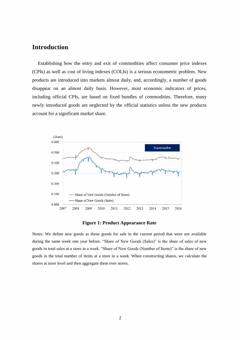
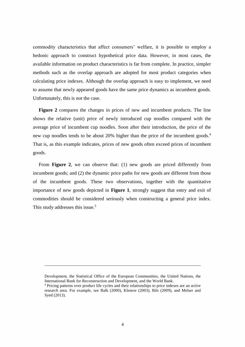
Figure 1: Product Appearance Rate
Notes: We define new goods as those goods for sale in the current period that were not available
during the same week one year before. “Share of New Goods (Sales)” is the share of sales of new
goods in total sales at a store in a week. “Share of New Goods (Number of Items)” is the share of new
goods in the total number of items at a store in a week. When constructing shares, we calculate the
shares at store level and then aggregate them over stores.
3
Figure 1 shows the weekly appearance rate of new products at supermarkets from our
point-of-sales (POS) data.1 More precisely, it shows the share, within total products, of
the products that did not exist during the same week in the previous year, in terms of both
the number of items and the proportion of sales. Measured by sales, new products
account for about 35% of all products, whereas, in terms of the number of items, new
products occupy more than 40% of the total sales.2 Accordingly, by limiting the product
bundle to products that have been available in the market for more than one year, a
significant quantity of sales information is neglected.
Although official CPIs are based on a limited number of products, most economic
data, including consumer expenditure and company sales data, cover all products that are
traded. In other words, the price index is based largely on continuing goods, whereas
expenditure and sales data include new goods that have just entered markets. This
divergence in the product space between expenditure and the price index could cause
serious inconsistency when constructing “real” economic variables if new goods are
priced differently to incumbent goods.
The treatment of new products has been one of the most important issues in
constructing price indexes. In the long history of price index theory, commencing with
the seminal works of Fisher (1922), almost all of the index formula considered require at
least two or more price data at distinct times or places so that we can calculate the price
relatives, the ratio of the prices for the same commodity at two different times or places.
Quite obviously, without multiple observations of prices, it is impossible to construct
most of the well-known price indexes, including the Laspeyres and Fisher indexes. One
of the commonly adopted approaches for handling newly appeared or disappeared goods
is to create hypothetical price data.3 If we have a complete set of information about
1 Section 4 describes the POS data in detail. 2 Figure 1 treats goods with identical commodity codes (the Japanese Article Number) sold at
different stores as different commodities. Therefore, the product appearance rate does not
necessarily correspond to the appearance rate of newly released products from manufacturers. 3 See Consumer Price Index Manual: Theory and Practice (2004, Chapter 8) by the
International Labor Organization, the Organisation for Economic Co-operation and
4
commodity characteristics that affect consumers’ welfare, it is possible to employ a
hedonic approach to construct hypothetical price data. However, in most cases, the
available information on product characteristics is far from complete. In practice, simpler
methods such as the overlap approach are adopted for most product categories when
calculating price indexes. Although the overlap approach is easy to implement, we need
to assume that newly appeared goods have the same price dynamics as incumbent goods.
Unfortunately, this is not the case.
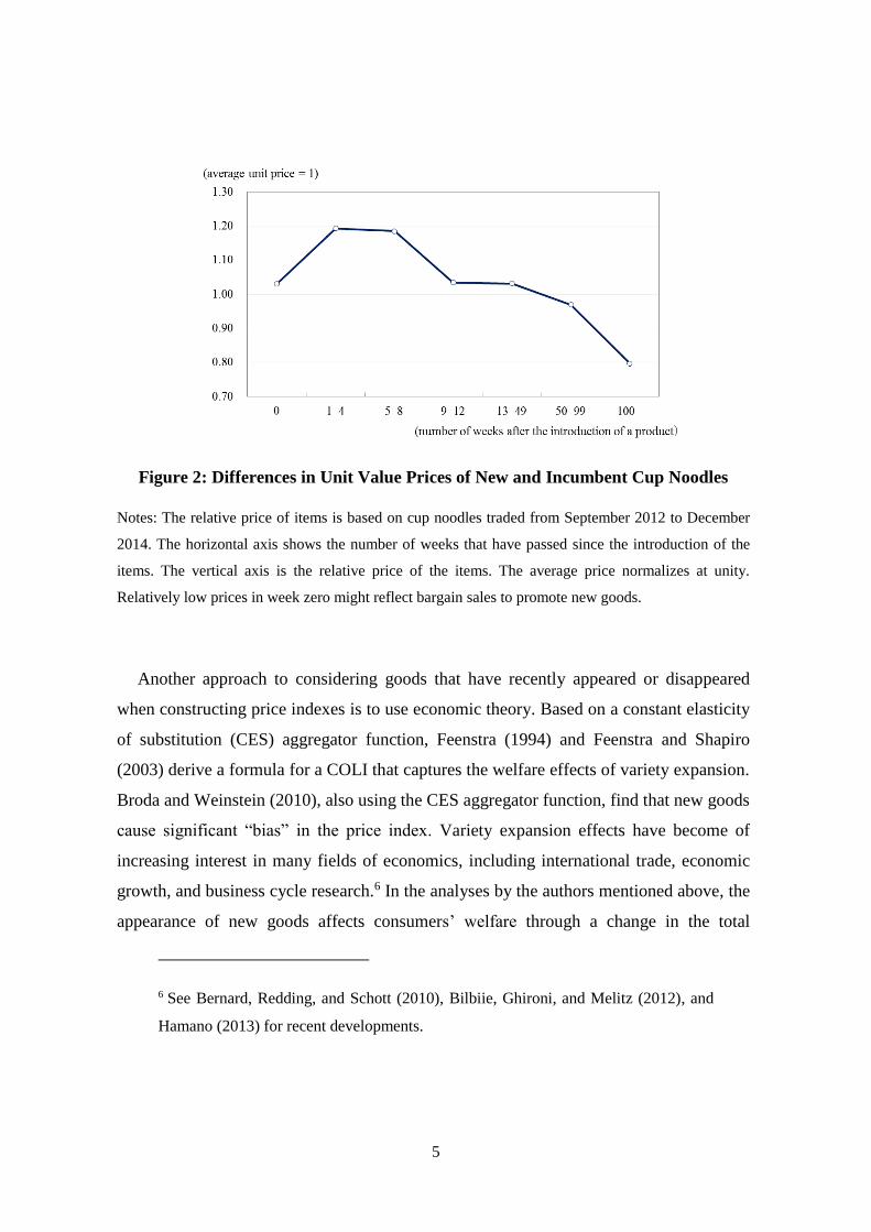
Figure 2 compares the changes in prices of new and incumbent products. The line
shows the relative (unit) price of newly introduced cup noodles compared with the
average price of incumbent cup noodles. Soon after their introduction, the price of the
new cup noodles tends to be about 20% higher than the price of the incumbent goods.4
That is, as this example indicates, prices of new goods often exceed prices of incumbent
goods.
From Figure 2, we can observe that: (1) new goods are priced differently from
incumbent goods; and (2) the dynamic price paths for new goods are different from those
of the incumbent goods. These two observations, together with the quantitative
importance of new goods depicted in Figure 1, strongly suggest that entry and exit of
commodities should be considered seriously when constructing a general price index.
This study addresses this issue.5
Development, the Statistical Office of the European Communities, the United Nations, the
International Bank for Reconstruction and Development, and the World Bank. 4 Pricing patterns over product life cycles and their relationships to price indexes are an active
research area. For example, see Balk (2000), Klenow (2003), Bils (2009), and Melser and
Syed (2013).
5
Figure 2: Differences in Unit Value Prices of New and Incumbent Cup Noodles
Notes: The relative price of items is based on cup noodles traded from September 2012 to December
2014. The horizontal axis shows the number of weeks that have passed since the introduction of the
items. The vertical axis is the relative price of the items. The average price normalizes at unity.
Relatively low prices in week zero might reflect bargain sales to promote new goods.
Another approach to considering goods that have recently appeared or disappeared
when constructing price indexes is to use economic theory. Based on a constant elasticity
of substitution (CES) aggregator function, Feenstra (1994) and Feenstra and Shapiro
(2003) derive a formula for a COLI that captures the welfare effects of variety expansion.
Broda and Weinstein (2010), also using the CES aggregator function, find that new goods
cause significant “bias” in the price index. Variety expansion effects have become of
increasing interest in many fields of economics, including international trade, economic
growth, and business cycle research.6 In the analyses by the authors mentioned above, the
appearance of new goods affects consumers’ welfare through a change in the total
6 See Bernard, Redding, and Schott (2010), Bilbiie, Ghironi, and Melitz (2012), and
Hamano (2013) for recent developments.
6
number of product varieties, not through price differentials between new and incumbent
goods. Although the variety channel is certainly important, other effects, including the
introduction of commodities with higher/lower prices or qualities, can have a major
impact on consumer welfare and the general price level. For example, assume that a firm
replaces its old product with a new product of the same quality but with a higher price.
Ceteris paribus, consumers’ welfare will decrease and the true COLIs will increase.
However, as the total number of product varieties is unchanged, the COLIs constructed
by Feenstra (1994) will remain unchanged, despite the fact that consumers’ welfare
decreases.
Rather than focusing on the variety expansion effects, the present study considers the
effects on the price index of the price differentials between new products and incumbent
products. More precisely, we construct a unit value price index (UVPI) that covers all
products, including new goods. The change in the UVPI is decomposed into: (1) standard
price change effects that are identical to the changes in the Laspeyres price indexes; (2)
substitution effects within the continuing goods category that reflect changes in the share
of commodities; and (3) turnover/new product effects that capture the contribution of the
price differentials between new and incumbent goods. This decomposition is an extension
of the previous studies by Silver (2009, 2010) and Diewert and Von der Lippe (2010),
which consider continuing goods, but exclude our third effects, the turnover/new product
effects.
If the differences in quality between new and existing goods are negligible, the price
differentials between new and incumbent goods affect COLIs in a straightforward
manner. On the other hand, if there are substantial changes in quality between the new
and incumbent goods, the price differences will mainly be a reflection of the quality
differences. In such a case, the third effects (the turnover/new product effects) can be
offset by the differences in quality in terms of their impact on consumers’ welfare.
Unfortunately, without detailed information on product characteristics, it is impossible to
identify the importance of quality differences. That is, the third effects tell us the two
extreme cases. If price differences between new and incumbent goods are very small after
7
controlling for quality differences, the sum of the first and second effects can be regarded
as the unbiased estimates of the true CPI. On the other hand, if the newly appeared goods
are of the same quality as the old goods, but have higher/lower prices, the third effects
contain very important information on consumers’ welfare that is not captured by the
conventional price indexes based on continuing goods, or by the COLIs based on variety
expansion effects. We suspect that the effects of the quality differentials between the new
and incumbent goods lie between the two extreme cases. That is, our estimates of the
UVPI with the turnover/new product effects provide upper limit estimates of the true CPI
if the quality of the new goods is no worse than that of the incumbent goods.7
In the empirical part of this study, which is based on weekly scanner data collected in
4,000 retail stores across Japan, we show that a decomposition of the data into these three
effects above reveals that the turnover/new product effects are generally nonnegligible.
The effects became very large during 2007, 2008, and the period after 2014, so that the
discrepancies between the UVPI and other price indexes and COLIs became significant.
During these periods, input prices for companies increased because of the depreciation of
the currency and the surge in material prices. Rather than increasing the tag price of
incumbent goods, it is possible that companies introduced new goods of a similar quality
and price to the old but of a smaller size or quantity to obscure the price increase. Section
6 discusses the relation between quality and price changes during those periods in detail.
The rest of the paper proceeds as follows. In Section 2, we review the COLIs with
product turnover developed by Feenstra (1994) and Broda and Weinstein (2010) to
inform our calculation of COLIs based on the POS data in a later section. Section 3
explains our UVPI and the decomposition of the UVPI into the three price change effects.
Section 4 describes the scanner data used in this study. In Section 5, we compare and
discuss the results of the UVPI and COLIs with product turnover and conventional price
indexes. Section 6 discusses some cases of actual product turnover to illustrate the
possible effects of quality differences. The final section concludes the paper.
7 It is also possible that new goods are lower quality and have higher prices than incumbent
goods. In such a case, the turnover/new goods effect is lower than the true price effects.
8
I. Cost of Living Index with Product Turnover
The seminal work of Feenstra (1994) develops the concept of the COLI with product
variety, based on the CES-type utility function. Broda and Weinstein (2010) extend the
COLI to include the effects of brand variety. In this section, we review the COLIs
developed by Feenstra (1994) and Broda and Weinstein (2010).
A. Feenstra’s Cost of Living Index
We start by describing the CES utility function of the representative consumer. The
upper level utility function, 𝑈𝑡, at time t is specified as follows:
𝑈𝑡 = (∑ 𝛽𝑔𝑡(𝐶𝑡𝑔𝑡)
𝜎−1𝜎
𝑔𝑡∈𝐺
)
𝜎𝜎−1
,
where 𝐶𝑡𝑔𝑡 is the aggregate consumption of product group 𝑔𝑡 ∈ 𝐺 , 𝛽𝑔 is the weight of
category 𝑔𝑡 in the CES utility function, and 𝐺 is the set of all product groups. Note that
we allow the elements of each product group set, 𝑔𝑡, to vary over time. That is, in each
group, new commodities could emerge and other goods disappear, so that the total
number of commodities in the set 𝑔𝑡 is not constant over time. 𝜎 is the CES across
product groups for demand. The lower level of the utility function is:
𝐶𝑡𝑔𝑡 = (∑𝛼𝑖(𝑞𝑡
𝑖)
𝜎𝑔−1
𝜎𝑔
𝑖∈𝑔𝑡
)
𝜎𝑔𝜎𝑔−1
,
where 𝑞𝑡𝑖 is the consumption quantity of the individual goods index 𝑖 ∈ 𝑔𝑡, and 𝛼𝑖 is the
weight of goods 𝑖 in the CES aggregator. 𝜎𝑔 is the CES within product group 𝑔𝑡 for
9
demand.8 Solving the optimization problem of the consumer, we obtain the unit cost
function of 𝐶𝑡𝑔𝑡 as follows:
𝐸(𝑝𝑡, 𝑔𝑡)
𝐶𝑡𝑔𝑡
= (∑ 𝛼𝑖𝜎(𝑝𝑡
𝑖)1−𝜎𝑔
𝑖∈𝑔𝑡
)
11−𝜎𝑔
,
where 𝑝𝑡 is the vector of individual prices and 𝑝𝑡𝑖 is the price of the individual goods
index, 𝑖 ∈ 𝑔𝑡. The COLI of product group 𝑔𝑡 can be written as:
𝐶𝑂𝐿𝐼(𝑝𝑡, 𝑝𝑡−𝑦, 𝑔𝑡, 𝑔𝑡−𝑦) =𝐸(𝑝𝑡, 𝑔𝑡)
𝐸(𝑝𝑡−𝑦, 𝑔𝑡−𝑦).
Sato (1976) and Vartia (1976) show that the above COLI can be calculated without
estimating the values of 𝛼𝑖 and 𝜎𝑔 if the sets of individual product groups are the same
between the current and base period: that is, if 𝑔𝑡 = 𝑔𝑡−𝑦 = 𝑔. The exact price index,
𝑃𝐼𝑆𝑉(𝑝𝑡, 𝑝𝑡−𝑦, 𝑔), can be formulated as follows:
𝐸(𝑝𝑡, 𝑔)
𝐸(𝑝𝑡−𝑦, 𝑔)=∏(
𝑝𝑡𝑖
𝑝𝑡−𝑦𝑖)
𝜙𝑡𝑖(𝑔)
𝑖∈𝑔
≡ 𝑃𝐼𝑆𝑉(𝑝𝑡, 𝑝,𝑡−𝑦, 𝑔),
where
𝜙𝑡𝑖(𝑔) =
(𝑤𝑡𝑖(𝑔) − 𝑤𝑡−𝑦
𝑖 (𝑔)
ln (𝑤𝑡𝑖(𝑔)) − ln (𝑤𝑡−𝑦
𝑖 (𝑔)))
∑ (𝑤𝑡𝑖(𝑔) − 𝑤𝑡−𝑦
𝑖 (𝑔)
ln (𝑤𝑡𝑖(𝑔)) − ln (𝑤𝑡−𝑦
𝑖 (𝑔)))𝑖∈𝑔
, and 𝑤𝑡𝑖(𝑔) =
𝑝𝑡𝑖𝑞𝑡𝑖
∑ 𝑝𝑡𝑖𝑞𝑡𝑖
𝑖∈𝑔
.
It is possible to obtain the aggregate-level Sato–Vartia-type COLI, as follows:
𝑃𝐼𝑡SV =∏[𝑃𝐼𝑆𝑉(𝑝𝑡, 𝑝𝑡−𝑦, 𝑔𝑡,𝑡−𝑦)]
𝜙𝑡𝑔
𝑔∈𝐺
, (1)
8 To be precise, 𝜎𝑔 should be denoted as 𝜎𝑔𝑡 because the goods category varies over time. To
keep the expression simple, we omit the subscript t from 𝜎𝑔𝑡.
10
where
𝜙𝑡𝑔=
(𝑤𝑡𝑔− 𝑤𝑡−𝑦
𝑔
ln(𝑤𝑡𝑔) − ln (𝑤𝑡−𝑦
𝑔))
∑ (𝑤𝑡𝑔− 𝑤𝑡−𝑦
𝑔
ln(𝑤𝑡𝑔) − ln (𝑤𝑡−𝑦
𝑔))𝑔∈𝐺
, where 𝑤𝑡𝑔=
∑ 𝑝𝑡𝑖𝑞𝑡𝑖
𝑖∈𝑔𝑡,𝑡−𝑦
∑ ∑ 𝑝𝑡𝑖𝑞𝑡𝑖
𝑖∈𝑔𝑡,𝑡−𝑦𝑔∈𝐺
.
Based on Sato (1976) and Vartia (1976), Feenstra (1994) develops the concept of the
COLI for the case in which sets of individual products are not the same between the
current period and the base period: that is, 𝑔𝑡 ≠ 𝑔𝑡−𝑦 . Feenstra’s COLI is defined as
follows:
𝐸(𝑝𝑡, 𝑔𝑡)
𝐸(𝑝𝑡−𝑦, 𝑔𝑡−𝑦)= 𝑃𝐼𝑆𝑉
𝑔(𝑝𝑡, 𝑝𝑡−𝑦, 𝑔𝑡,𝑡−𝑦)(
𝜆𝑔𝑡cr
𝜆𝑔𝑡bs)
1𝜎𝑔−1
≡ 𝑃𝐹(𝑝𝑡, 𝑝𝑡−𝑦, 𝑔𝑡, 𝑔𝑡−𝑦),
where
𝑔𝑡,𝑡−𝑦 = 𝑔𝑡 ∩ 𝑔𝑡−𝑦,
𝜆𝑔𝑡cr =
∑ 𝑝𝑡𝑖𝑞𝑡𝑖
𝑖∈𝑔𝑡,𝑡−𝑦
∑ 𝑝𝑡𝑖𝑞𝑡𝑖
𝑖∈𝑔𝑡
, 𝜆𝑔𝑡bs =
∑ 𝑝𝑡−𝑦𝑖 𝑞𝑡−𝑦
𝑖𝑖∈𝑔𝑡,𝑡−𝑦
∑ 𝑝𝑡−𝑦𝑖 𝑞𝑡−𝑦
𝑖𝑖∈𝑔𝑡−𝑦
.
The term 𝜆𝑔𝑡cr denotes the sales share of the surviving goods between the current and
base periods in the current period t, whereas 𝜆𝑔𝑡bs is the sales share of surviving goods
between the current and base periods in the base period, t–y. When the set of product
groups changes, Feenstra’s COLI becomes the product of the exact price index based on
𝑔𝑡,𝑡−𝑦 and the term (𝜆𝑔𝑡cr 𝜆𝑔𝑡
bs⁄ )1
𝜎𝑔−1 , which is known as the group-level lambda ratio,
adjusted by 𝜎𝑔. Note that, unlike the Sato–Vartia-type COLI, to obtain the lambda ratio,
we require information on the elasticity of substitution for demand within a group.
The aggregate-level COLI based on Feenstra (1994), 𝑃𝐼𝑡F, is given by the following
expression:
11
𝑃𝐼𝑡F =∏[𝑃𝐼𝑆𝑉(𝑝𝑡, 𝑝𝑡−𝑦, 𝑔𝑡,𝑡−𝑦) (
𝜆𝑔𝑡cr
𝜆𝑔𝑡bs)
1𝜎𝑔−1
]
𝜙𝑡𝑔
.
𝑔∈𝐺
(2)
B. Broda–Weinstein’s Cost of Living Index
Based on Feenstra (1994), Broda and Weinstein (2010) extend the COLI by taking
account of within-brand and across-brand variety. In other words, in addition to product
variety effects, Broda and Weinstein (2010) consider brand expansion effects. Their
COLI has three layers: brand-level, product group-level, and aggregate-level COLIs. The
brands are the lower layer in the product groups. The set of brands that change over time
is denoted as 𝑏𝑡, which is a subset of 𝑔𝑡.
The aggregate-level COLI based on Broda and Weinstein (2010), 𝑃𝐼𝑡𝐵𝑊, is defined as
follows:
𝑃𝐼𝑡BW = ∏
{
∏ [𝑃𝐼𝑆𝑉(𝑝𝑡, 𝑝𝑡−𝑦, 𝑏𝑡,𝑡−𝑦)(
𝜆𝑏𝑡cr
𝜆𝑏𝑡bs)
1𝜎𝑤𝑏(𝑏)−1
]
𝜙𝑡𝑤𝑏(𝑏)
𝑏∈ 𝑔𝑡 𝑔𝑡∈𝐺
×(𝜆𝑔𝑡cr
𝜆𝑔𝑡bs)
1𝜎𝑎𝑏(𝑔𝑡)−1
}
𝜙𝑡𝑎𝑏(𝑔𝑡)
,
(3)
where 𝑃𝐼𝑆𝑉(𝑝𝑡, 𝑝𝑡−𝑦, 𝑏𝑡,𝑡−𝑦) is the brand-level Sato–Vartia-type COLI. 𝜎𝑤𝑏(𝑏) is the
substitution elasticity of demand within brands in brand 𝑏, and 𝜎𝑎𝑏(𝑏) is the substitution
elasticity of demand across brands in product group 𝑔𝑡. (𝜆𝑏𝑡cr 𝜆𝑏𝑡
bs⁄ )1
𝜎𝑤𝑏(𝑏)−1 is the brand-
level lambda ratio adjusted by 𝜎𝑤𝑏(𝑏) , whereas (𝜆𝑔𝑡cr 𝜆𝑔𝑡
bs⁄ )1
𝜎𝑎𝑏(𝑔)−1 is the group-level
lambda ratio adjusted by 𝜎𝑎𝑏(𝑔). The parameters, 𝜆𝑏𝑡cr , 𝜆𝑏𝑡
bs , 𝜆𝑔𝑡cr , and 𝜆𝑔𝑡
bs , are defined,
respectively, as follows:
𝜆𝑏𝑡cr =
∑ 𝑝𝑡𝑖𝑞𝑡𝑖
𝑖∈𝑏𝑡,𝑡−𝑦
∑ 𝑝𝑡𝑖𝑞𝑡𝑖
𝑖∈𝑏𝑡
, 𝜆𝑏𝑡bs =
∑ 𝑝𝑡−𝑦𝑖 𝑞𝑡−𝑦
𝑖𝑖∈𝑏𝑡,𝑡−𝑦
∑ 𝑝𝑡−𝑦𝑖 𝑞𝑡−𝑦
𝑖𝑖∈𝑏𝑡−𝑦
,
12
𝜆𝑔𝑡cr =
∑ ∑ 𝑝𝑡𝑖𝑞𝑡𝑖
𝑖∈𝑏𝑡,𝑡−𝑦𝑏∈𝑔𝑡,𝑡−𝑦
∑ ∑ 𝑝𝑡𝑖𝑞𝑡𝑖
𝑖∈𝑏𝑡𝑏∈𝑔𝑡
, 𝜆𝑔𝑡bs =
∑ ∑ 𝑝𝑡−𝑦𝑖 𝑞𝑡−𝑦
𝑖𝑖∈𝑏𝑡,𝑡−𝑦𝑖∈𝑔𝑡,𝑡−𝑦
∑ ∑ 𝑝𝑡−𝑦𝑖 𝑞𝑡−𝑦
𝑖𝑖∈𝑏𝑡−𝑦𝑖∈𝑔𝑡−𝑦
.
𝜙𝑡𝑤𝑏(𝑏) and 𝜙𝑡
𝑎𝑏(𝑔) are defined, respectively, as follows:
𝜙𝑡𝑤𝑏(𝑏) =
(𝑤𝑡𝑏−𝑤𝑡−𝑦
𝑏
ln(𝑤𝑡𝑏)−ln(𝑤𝑡−𝑦
𝑏 ))
∑ (𝑤𝑡𝑏−𝑤𝑡−𝑦
𝑏
ln(𝑤𝑡𝑏)−ln(𝑤𝑡−𝑦
𝑏 ))𝑏∈𝑔
, where 𝑤𝑡𝑏 =
∑ 𝑝𝑡𝑖𝑞𝑡𝑖
𝑖∈𝑏𝑡,𝑡−𝑦
∑ ∑ 𝑝𝑡𝑖𝑞𝑡𝑖
𝑖∈𝑏𝑡,𝑡−𝑦𝑏∈𝑔,
𝜙𝑡𝑎𝑏(𝑔) =
(�̃�𝑡𝑔− �̃�𝑡−𝑦
𝑔
ln(�̃�𝑡𝑔) − ln(�̃�𝑡−𝑦
𝑔))
∑ (�̃�𝑡𝑔− �̃�𝑡−𝑦
𝑔
ln(�̃�𝑡𝑔) − ln(�̃�𝑡−𝑦
𝑔))𝑔∈𝐺
, where �̃�𝑡𝑔=
∑ ∑ 𝑝𝑡𝑖𝑞𝑡𝑖
𝑖∈𝑏𝑡,𝑡−𝑦𝑏∈𝑔𝑡,𝑡−𝑦
∑ ∑ ∑ 𝑝𝑡𝑖𝑞𝑡𝑖
𝑖∈𝑏𝑡,𝑡−𝑦𝑏∈𝑔𝑡,𝑡−𝑦𝑔∈𝐺
.
To calculate the Broda–Weinstein COLI, we need to estimate the elasticities of
substitution for demand both within and across brands in a category from the data.
II. Decomposition of the Unit Value Price Index
In this section, we define the UVPI and demonstrate the procedure for decomposing
changes in the rate of the UVPI into the effects of a standard product-level price change
within continuing goods, the substitution effects within continuing goods, and the
turnover/new product effects. That is, this section presents and discusses a formula that
describes the inflation rate of the UVPI as the weighted sum of the three effects, as
follows:
𝐈𝐧𝐟𝐥𝐚𝐭𝐢𝐨𝐧 𝐑𝐚𝐭𝐞 𝐨𝐟 𝐔𝐧𝐢𝐭 𝐕𝐚𝐥𝐮𝐞 𝐏𝐫𝐢𝐜𝐞 𝐈𝐧𝐝𝐞𝐱
= 𝐚𝟏 ×𝐏𝐫𝐢𝐜𝐞 𝐂𝐡𝐚𝐧𝐠𝐞 𝐄𝐟𝐟𝐞𝐜𝐭𝐬 + 𝐚𝟐 ×𝐒𝐮𝐛𝐬𝐭𝐢𝐭𝐮𝐭𝐢𝐨𝐧 𝐄𝐟𝐟𝐞𝐜𝐭𝐬
+ 𝐚𝟑 ×𝐓𝐮𝐫𝐧𝐨𝐯𝐞𝐫 𝐄𝐟𝐟𝐞𝐜𝐭𝐬 + 𝐚𝟒 ×𝐂𝐫𝐨𝐬𝐬 𝐓𝐞𝐫𝐦.
A. Unit Value Price Index as a Cost of Living Index
Assume that the representative consumer obtains utility from the total sum of
consumption volume, that is, all the consumption goods are perfect substitutes in each

13
category. For example, although a 500 ml orange juice package and a 1000 ml orange
juice package of the same brand are distinguished from the perspective of their Universal
Product Codes, their contents are virtually the same. We assume that the consumption of
these two orange juice packages gives the same utility level to a consumer as does the
consumption of a 1500 ml package of orange juice of the same brand. Under the
assumption of perfect substitution within the category, we can measure the price level of
one category as the UVPI.
More concretely, we assume that the utility function of the representative consumer
has the following two layers:
𝑈𝑡 = (∑ 𝛽𝑔 (𝐶𝑡𝑔𝑡)
𝜎−1𝜎
𝑔𝑡∈𝐺
)
𝜎𝜎−1
,
𝐶𝑡𝑔𝑡 = ∑ 𝑣𝑖𝑞𝑡
𝑖
𝑖∈𝑔𝑡
,
where 𝑣𝑖 is the volume of product 𝑖.
Then, the unit cost of product group 𝑃𝑡𝑈(𝑔) can be written as:
𝑃𝑡𝑈(𝑔) =
𝐸(𝑝𝑡, 𝑞𝑡, 𝑣, 𝑔𝑡)
𝐶𝑡𝑔𝑡
= ∑ (𝑣𝑖𝑞𝑡
𝑖
∑ 𝑣𝑖𝑞𝑡𝑖
𝑖∈𝑔𝑡
)𝑝𝑡𝑖
𝑣𝑖𝑖∈𝑔𝑡
,
where 𝑣 is a vector of 𝑣𝑖 , 𝑖 ∈ 𝑔.
The UVPI is defined as:
𝑃𝐼𝑈(𝑝𝑡, 𝑝𝑡−𝑦, 𝑞𝑡, 𝑞𝑡−𝑦, 𝑔𝑡, 𝑔𝑡−𝑦) =𝑃𝑡𝑈(𝑔𝑡)
𝑃𝑡−𝑦𝑈 (𝑔𝑡−𝑦)
.
The aggregate-level COLI is given by the following expression:
𝑃𝐼𝑡U =∏[𝑃𝐼𝑈(𝑝𝑡, 𝑝𝑡−𝑦, 𝑞𝑡, 𝑞𝑡−𝑦, 𝑔𝑡, 𝑔𝑡−𝑦)]
𝜙𝑡𝑔𝑢
𝑔∈𝐺
, (4)
where
14
𝜙𝑡𝑔𝑢=
(𝑤𝑡𝑔𝑢− 𝑤𝑡−𝑦
𝑔𝑢
ln(𝑤𝑡𝑔𝑢) − ln (𝑤𝑡−𝑦
𝑔𝑢))
∑ (𝑤𝑡𝑔𝑢− 𝑤𝑡−𝑦
𝑔𝑢
ln(𝑤𝑡𝑔𝑢) − ln (𝑤𝑡−𝑦
𝑔𝑢))𝑔∈𝐺
and 𝑤𝑡𝑔𝑢=
∑ 𝑝𝑡𝑖𝑞𝑡𝑖
𝑖∈𝑔𝑡
∑ ∑ 𝑝𝑡𝑖𝑞𝑡𝑖
𝑖∈𝑔𝑡𝑔∈𝐺
.
B. New Goods, Old Goods, and Continuing Goods
To capture the effects of the changes in the product space, first, we classify all
products in category 𝑔𝑡 into three groups: (1) new goods, (2) old goods, and (3)
continuing goods. Consider two periods, the current period 𝑡 and the base period 𝑡 – 𝑦,
where 𝑦 is a fixed time interval, such as one year. An individual product 𝑖 is defined as a
“new good” in period 𝑡 if the product exists in period 𝑡 but not in period 𝑡 – 𝑦. Similarly,
an individual product 𝑖 is defined as an “old good” in period 𝑡 if the product does not
exist in period 𝑡 but exists in period 𝑡 – 𝑦 . An individual product 𝑖 is defined as a
“continuing good” in period t if the product exists in both period 𝑡 and period 𝑡 – 𝑦. 𝑔𝑡𝑁,
𝑔𝑡𝑂, and 𝑔𝑡,𝑡−𝑦 denote the set of new goods, the set of old goods, and the set of continuing
goods, respectively, in category 𝑔 in period 𝑡. By construction, the set of available goods
at time t in category 𝑔, 𝑔𝑡 is a union of the new goods and continuing goods: that is,
𝑔𝑡=𝑔𝑡𝑁 ∪ 𝑔𝑡,𝑡−𝑦. Similarly, the continuing goods can be defined as the intersection of 𝑔𝑡
and 𝑔𝑡−𝑦 : that is, 𝑔𝑡,𝑡−𝑦 = 𝑔𝑡 ∩ 𝑔𝑡−𝑦. It is straightforward to derive the following
relations:
𝑔𝑡𝑁 = 𝑔𝑡\𝑔𝑡,𝑡−𝑦,
𝑔𝑡𝑂 = 𝑔𝑡−𝑦\𝑔𝑡,𝑡−𝑦.
C. Unit Value Price Indexes for New Goods, Old Goods, and Continuing Goods
Let us denote the quantity and price of item 𝑖 sold in period 𝑡 as 𝑞𝑡𝑖 and 𝑝𝑡
𝑖 ,
respectively. 𝑣𝑖 denotes the volume of product 𝑖. The total unit value price of category 𝑔
in period 𝑡, 𝑃𝑡𝑈(𝑔), can be expressed as the weighted sum of the unit value price of
continuing goods, 𝑃𝑡𝑈𝐶(𝑔), and that of new goods, 𝑃𝑡
𝑈𝑁(𝑔).
15
𝑃𝑡𝑈(𝑔) = ∑ (
𝑣𝑖𝑞𝑡𝑖
∑ 𝑣𝑖𝑞𝑡𝑖
𝑖∈𝑔𝑡
)𝑝𝑡𝑖
𝑣𝑖𝑖∈𝑔𝑡
= (∑ 𝑣𝑖𝑞𝑡
𝑖𝑖∈𝑔𝑡,𝑡−𝑦
∑ 𝑣𝑖𝑞𝑡𝑖
𝑖∈𝑔𝑡
) ∑ (𝑣𝑖𝑞𝑡
𝑖
∑ 𝑣𝑖𝑞𝑡𝑖
𝑖∈𝑔𝑡,𝑡−𝑦
)𝑝𝑡𝑖
𝑣𝑖𝑖∈𝑔𝑡,𝑡−𝑦
+ (∑ 𝑣𝑖𝑞𝑡
𝑖𝑖∈𝑔𝑡
𝑁
∑ 𝑣𝑖𝑞𝑡𝑖
𝑖∈𝑔𝑡
) ∑ (𝑣𝑖𝑞𝑡
𝑖
∑ 𝑣𝑖𝑞𝑡𝑖
𝑖∈𝑔𝑡𝑁
)𝑝𝑡𝑖
𝑣𝑖𝑖∈𝑔𝑡
𝑁
= 𝑤𝑡𝐶(𝑔)𝑃𝑡
𝑈𝐶(𝑔) + 𝑤𝑡𝑁(𝑔)𝑃𝑡
𝑈𝑁(𝑔),
where
𝑤𝑡𝐶 (𝑔) =
∑ 𝑣𝑖𝑞𝑡𝑖
𝑖∈𝑔𝑡,𝑡−𝑦
∑ 𝑣𝑖𝑞𝑡𝑖
𝑖∈𝑔𝑡
, 𝑤𝑡𝑁(𝑔) =
∑ 𝑣𝑖𝑞𝑡𝑖
𝑖∈𝑔𝑡𝑁
∑ 𝑣𝑖𝑞𝑡𝑖
𝑖∈𝑔𝑡
,
𝑃𝑡𝑈𝐶(𝑔) = ∑ (
𝑣𝑖𝑞𝑡𝑖
∑ 𝑣𝑖𝑞𝑡𝑖
𝑖∈𝑔𝑡,𝑡−𝑦
)𝑝𝑡𝑖
𝑣𝑖𝑖∈𝑔𝑡,𝑡−𝑦
, and 𝑃𝑡𝑈𝑁(𝑔) = ∑ (
𝑣𝑖𝑞𝑡𝑖
∑ 𝑣𝑖𝑞𝑡𝑖
𝑖∈𝑔𝑡𝑁
)𝑝𝑡𝑖
𝑣𝑖𝑖∈𝑔𝑡
𝑁
.
Similarly, we can construct the UVPI in period 𝑡 – 𝑦, 𝑃𝑡−𝑦𝑈 (𝑔), as the weighted sum of
the unit value prices of continuing goods, 𝑃𝑡−𝑦𝑈𝐶 (𝑔), and of old goods, 𝑃𝑡−𝑦
𝑈𝑂 (𝑔).
𝑃𝑡−𝑦𝑈 (𝑔) ≡ ∑ (
𝑣𝑖𝑞𝑡−𝑦𝑖
∑ 𝑣𝑖𝑞𝑡−𝑦𝑖
𝑖∈𝑔𝑡−𝑦
)𝑝𝑡−𝑦𝑖
𝑣𝑖𝑖∈𝑔𝑡−𝑦
= (∑ 𝑣𝑖𝑞𝑡−𝑦
𝑖𝑖∈𝑔𝑡,𝑡−𝑦
∑ 𝑣𝑖𝑞𝑡−𝑦𝑖
𝑖∈𝑔𝑡−𝑦
) ∑ (𝑣𝑖𝑞𝑡−𝑦
𝑖
∑ 𝑣𝑖𝑞𝑡−𝑦𝑖
𝑖∈𝑔𝑡,𝑡−𝑦
)𝑝𝑡−𝑦𝑖
𝑣𝑖𝑖∈𝑔𝑡,𝑡−𝑦
+ (∑ 𝑣𝑖𝑞𝑡−𝑦
𝑖𝑖∈𝑔𝑡
𝑂
∑ 𝑣𝑖𝑞𝑡𝑖
𝑖∈𝑔𝑡−𝑦
) ∑ (𝑣𝑖𝑞𝑡−𝑦
𝑖
∑ 𝑣𝑖𝑞𝑡−𝑦𝑖
𝑖∈𝑔𝑡𝑂
)𝑝𝑡−𝑦𝑖
𝑣𝑖𝑖∈𝑔𝑡
𝑂
= 𝑤𝑡−𝑦𝐶 (𝑔)𝑃𝑡−𝑦
𝑈𝐶 (𝑔) + 𝑤𝑡−𝑦𝑂 (𝑔)𝑃𝑡−𝑦
𝑈𝑂 (𝑔),
where
𝑤𝑡−𝑦𝐶 (𝑔) =
∑ 𝑣𝑖𝑞𝑡−𝑦𝑖
𝑖∈𝑔𝑡,𝑡−𝑦
∑ 𝑣𝑖𝑞𝑡−𝑦𝑖
𝑖∈𝑔𝑡−𝑦
, 𝑤𝑡−𝑦𝑂 (𝑔) =
∑ 𝑣𝑖𝑞𝑡−𝑦𝑖
𝑖∈𝑔𝑡𝑂
∑ 𝑣𝑖𝑞𝑡−𝑦𝑖
𝑖∈𝑔𝑡−𝑦
,
16
𝑃𝑡−𝑦𝑈𝐶 (𝑔) = ∑ (
𝑣𝑖𝑞𝑡−𝑦𝑖
∑ 𝑣𝑖𝑞𝑡−𝑦𝑖
𝑖∈𝑔𝑡,𝑡−𝑦
)𝑝𝑡−𝑦𝑖
𝑣𝑖𝑖∈𝑔𝑡,𝑡−𝑦
, and 𝑃𝑡−𝑦𝑈𝑂 (𝑔) = ∑ (
𝑣𝑖𝑞𝑡−𝑦𝑖
∑ 𝑣𝑖𝑞𝑡−𝑦𝑖
𝑖∈𝑔𝑡𝑂
)𝑝𝑡−𝑦𝑖
𝑣𝑖𝑖∈𝑔𝑡
𝑂
.
D. Decomposition into Price Change, Substitution, and Turnover/New Goods Effects
The inflation rate of the UVPI can be written as follows:
𝑃𝑡𝑈(𝑔) − 𝑃𝑡−𝑦
𝑈 (𝑔)
𝑃𝑡−𝑦𝑈 (𝑔)
= (𝑃𝑡−𝑦𝑈𝐶 (𝑔)
𝑃𝑡−𝑦𝑈 (𝑔)
)𝑤𝑡𝐶(𝑔)𝑃𝑡
𝑈𝐶(𝑔) − 𝑤𝑡−𝑦𝐶 (𝐶)𝑃𝑡−𝑦
𝑈𝐶 (𝑔)
𝑃𝑡−𝑦𝑈𝐶 (𝑔)
+ (𝑃𝑡−𝑦𝑈𝑂 (𝑔)
𝑃𝑡−𝑦𝑈 (𝑔)
)𝑤𝑡𝑁(𝑔)𝑃𝑡
𝑈𝑁(𝑔) − 𝑤𝑡−𝑦𝑂 (𝑔)𝑃𝑡−𝑦
𝑈𝑂 (𝑔)
𝑃𝑡−𝑦𝑈𝑂 (𝑔)
.
Using the formula for the Laspeyres price index, 𝜋𝑡𝐿𝐶(𝑔), the substitution effect among
continuing goods, 𝜙t𝑈𝐶(𝑔),9 and the effects of product turnover, we can express the rate
of change of the UVPI as the weighted sum of the three price effects and the cross-term:10
𝑃𝑡𝑈(𝑔) − 𝑃𝑡−𝑦
𝑈 (𝑔)
𝑃𝑡−𝑦𝑈 (𝑔)
= (𝑃𝑡−𝑦𝑈𝐶 (𝑔)
𝑃𝑡−𝑦𝑈 (𝑔)
)𝑤𝑡−𝑦𝐶 (𝑔)𝜋𝑡
𝐿𝐶(𝑔) + (𝑃𝑡−𝑦𝑈𝐶 (𝑔)
𝑃𝑡−𝑦𝑈 (𝑔)
)𝑤𝑡−𝑦𝐶 (𝑔)𝜙𝑡
𝑈𝐶(𝑔)
+𝑤𝑡−𝑦𝑂 (𝑔)(𝑃𝑡
𝑈𝐶(𝑔) − 𝑃𝑡−𝑦𝑈𝑂 (𝑔)) + 𝑤𝑡
𝑁(𝑔)(𝑃𝑡𝑈𝑁(𝑔) − 𝑃𝑡
𝑈𝐶(𝑔))
𝑃𝑡−𝑦𝑈 (𝑔)
+ (𝑃𝑡−𝑦𝑈𝐶 (𝑔)
𝑃𝑡−𝑦𝑈 (𝑔)
)𝑤𝑡−𝑦𝐶 (𝑔)𝜙𝑡
𝑈𝐶(𝑔)𝜋𝑡𝑈𝐶(𝑔),
(5)
where 𝜋𝑡𝑈𝐶 = (𝑃𝑡
𝑈𝐶(𝑔) − 𝑃𝑡−𝑦𝑈𝐶 (𝑔)) 𝑃𝑡−𝑦
𝑈𝐶 (𝑔)⁄ , and
9 We follow the definition of Diewert and Von der Lippe (2010) in relation to the substitution
effect. This substitution effect can be written as the covariance between the change in the
volume share and relative prices. See A2 in Appendix A for details. 10 See Appendix A for the derivation.
17
𝜙𝑡𝑈𝐶(𝑔) =
∑ 𝑝𝑡𝑖[𝑠𝑡
𝑖−𝑠𝑡−𝑦𝑖 ]𝑖∈𝑔𝑡,𝑡−𝑦
∑ [𝑣𝑖𝑞𝑡
𝑖
∑ 𝑣𝑖𝑞𝑡𝑖
𝑖∈𝑔𝑡,𝑡−𝑦
×𝑝𝑡𝑖
𝑣𝑖]𝑖∈𝑔𝑡,𝑡−𝑦
, 𝑠𝑡𝑖 =
𝑣𝑖𝑞𝑡𝑖
∑ 𝑣𝑖𝑞𝑡𝑖
𝑖∈𝑔𝑡,𝑡−𝑦
.
The first term on the right-hand side (RHS) of (5) is the standard price change effect
measured by the Laspeyres formula. Note that if there were no product turnover, we
would obtain 𝑃𝑡−𝑦UC (𝑔) = 𝑃𝑡−𝑦
𝑈 (𝑔) and 𝑤𝑡−𝑦𝐶 (𝑔) = 1. Thus, the first term would be equal
to the standard rate of price change, 𝜋𝑡𝐿𝐶(𝑔). The second term represents the substitution
effects within the continuing goods category. If this term were negative, a product with a
relatively lower unit value price would increase its volume share. That is, the substitution
effect captures the degree to which demand shifts in response to the differences in relative
prices. The third term shows the contribution of product turnover to the UVPI. The
numerator of the third term is the weighted sum of the price differential between (1) new
goods and continuing goods, and (2) continuing goods and disappearing goods. Note that
𝑤𝑡−𝑦𝑂 (𝑔) is the ratio of disappearing goods within the total volume of goods sold in
period t − y, and 𝑃𝑡𝑈𝐶(𝑔) − 𝑃𝑡−𝑦
𝑈𝑂 (𝑔) shows the differences between the unit value prices
of continuing goods and old goods. In addition, note that 𝑤𝑡𝑁(𝑔) is the ratio of new goods
to the total volume of goods sold in period t, and that 𝑃𝑡𝑈𝑁(𝑔) − 𝑃𝑡
𝑈𝐶(𝑔) shows the
difference between the unit value prices of new and continuing goods. The third term is
interpreted as showing the substitution effects that occur through product turnover. The
final term represents the cross-effect of the substitution effects and price change effects
that are supposed to be quite small.
III. Point-of-Sales Data
In our empirical analyses, we use Japanese store-level weekly POS data, known as the
SRI,11 collected by INTAGE Inc. The data set contains information on weekly store-level
sales of processed foods, daily necessities, and cosmetics that have commodity codes and
11 SRI is the abbreviation for the Japanese “Syakaichosa-kenkyujo Retail Index,” which means
the “Retail Index by The Institute of Social Research.”
18
a Japanese Article Number.12 The sample period is between January 2006 and February
2016, which enables us to calculate the yearly rate of price changes that occur between
January 2007 and February 2016. The data set covers various types of stores, general
merchandise stores (GMSs), supermarkets, convenience stores, drug stores, and
specialized stores, including liquor shops, located across Japan. The data set contains
detailed information on the volume content of products, such as the number of washing
loads for which each box of laundry detergent can be used, as well as standard
information, including weight (milliliters or grams), the number of items, and the number
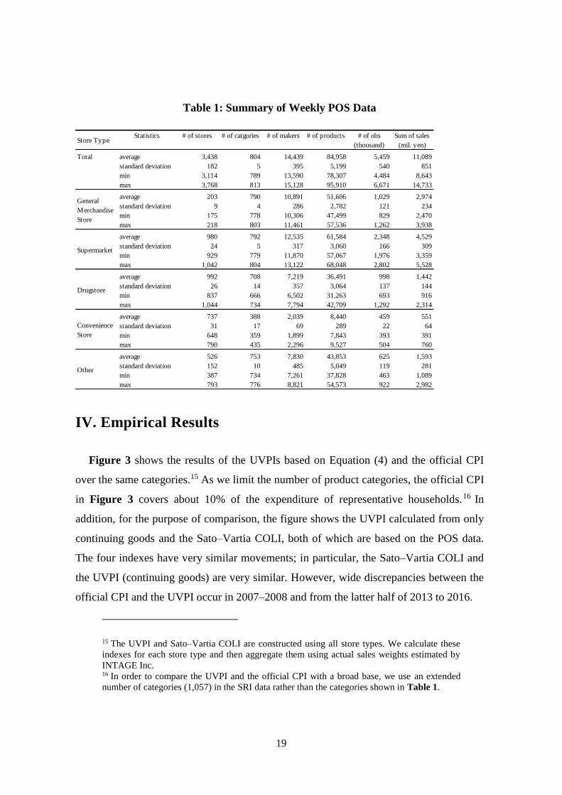
of meals for food products. Table 1 provides a detailed description of the data set used to
calculate the aggregated UVPI and the COLIs in the next section. The sales records
provide pretax price information. Our data set has 84,958 individual products and, on
average, more than five million observations per week.13
One noteworthy characteristic of the data set is its detailed commodity classification.
In the SRI data, commodities that have volume information are classified into more than
1,000 categories, which is about seven times more than the number of classifications
adopted by the Japanese official statistics. As Diewert and Von der Lippe (2010)
emphasize, when constructing a UVPI, aggregation over heterogeneous goods must be
avoided wherever possible. We expect that the highly detailed classification of our data
set will help to mitigate the aggregation bias indicated by Diewert and Von der Lippe
(2010). When calculating a UVPI, we take the average unit value price for each brand
and category, so that brand-level differences in quality are taken into account.14
12 Fresh foods are excluded from the data set because they lack commodity codes. 13 This summary table uses the same data that are used to calculate the Feenstra and Broda–
Weinstein COLIs. 14 To avoid the sample selection effect when calculating the rate of change of
individual product prices, we limit the store and category space to a range, such that
stores and product categories exist in both the current week and the same week of the
previous year.
19
Table 1: Summary of Weekly POS Data
IV. Empirical Results
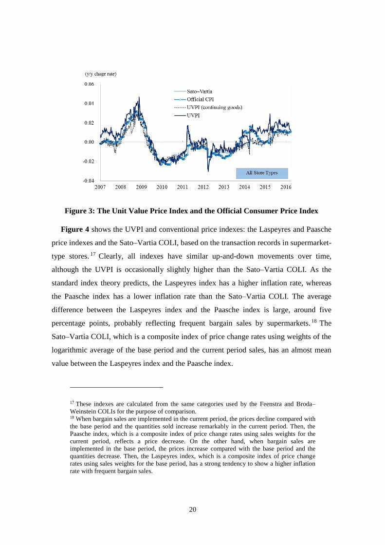
Figure 3 shows the results of the UVPIs based on Equation (4) and the official CPI
over the same categories.15 As we limit the number of product categories, the official CPI
in Figure 3 covers about 10% of the expenditure of representative households.16 In
addition, for the purpose of comparison, the figure shows the UVPI calculated from only
continuing goods and the Sato–Vartia COLI, both of which are based on the POS data.
The four indexes have very similar movements; in particular, the Sato–Vartia COLI and
the UVPI (continuing goods) are very similar. However, wide discrepancies between the
official CPI and the UVPI occur in 2007–2008 and from the latter half of 2013 to 2016.
15 The UVPI and Sato–Vartia COLI are constructed using all store types. We calculate these
indexes for each store type and then aggregate them using actual sales weights estimated by
INTAGE Inc. 16 In order to compare the UVPI and the official CPI with a broad base, we use an extended
number of categories (1,057) in the SRI data rather than the categories shown in Table 1.
Store TypeStatistics # of stores # of catgories # of makers # of products # of obs
(thousand)
Sum of sales
(mil. yen)
Total average 3,438 804 14,439 84,958 5,459 11,089
standard deviation 182 5 395 5,199 540 851
min 3,114 789 13,590 78,307 4,484 8,643
max 3,768 813 15,128 95,910 6,671 14,733
average 203 790 10,891 51,606 1,029 2,974
standard deviation 9 4 286 2,782 121 234
min 175 778 10,306 47,499 829 2,470
max 218 803 11,461 57,536 1,262 3,938
average 980 792 12,535 61,584 2,348 4,529
standard deviation 24 5 317 3,060 166 309
min 929 779 11,870 57,067 1,976 3,359
max 1,042 804 13,122 68,048 2,802 5,528
average 992 708 7,219 36,491 998 1,442
standard deviation 26 14 357 3,064 137 144
min 837 666 6,502 31,263 693 916
max 1,044 734 7,794 42,709 1,292 2,314
average 737 388 2,039 8,440 459 551
standard deviation 31 17 69 289 22 64
min 648 359 1,899 7,843 393 391
max 790 435 2,296 9,527 504 760
average 526 753 7,830 43,853 625 1,593
standard deviation 152 10 485 5,049 119 281
min 387 734 7,261 37,828 463 1,089
max 793 776 8,821 54,573 922 2,982
General
Merchandise
Store
Supermarket
Drugstore
Convenience
Store
Other
20
Figure 3: The Unit Value Price Index and the Official Consumer Price Index
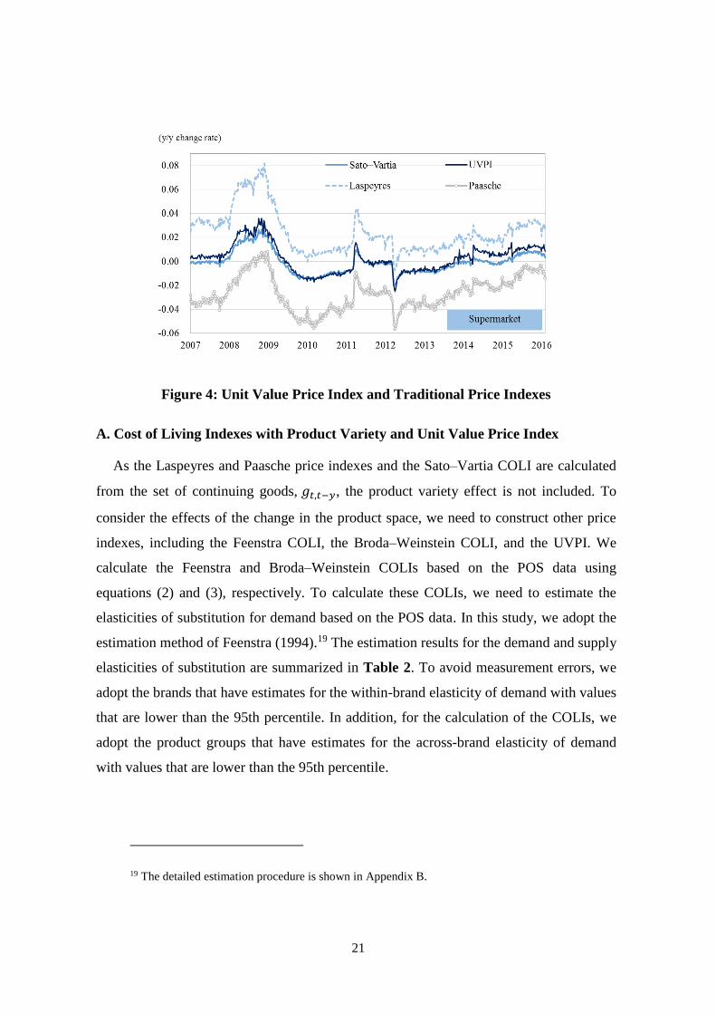
Figure 4 shows the UVPI and conventional price indexes: the Laspeyres and Paasche
price indexes and the Sato–Vartia COLI, based on the transaction records in supermarket-
type stores. 17 Clearly, all indexes have similar up-and-down movements over time,
although the UVPI is occasionally slightly higher than the Sato–Vartia COLI. As the
standard index theory predicts, the Laspeyres index has a higher inflation rate, whereas
the Paasche index has a lower inflation rate than the Sato–Vartia COLI. The average
difference between the Laspeyres index and the Paasche index is large, around five
percentage points, probably reflecting frequent bargain sales by supermarkets. 18 The
Sato–Vartia COLI, which is a composite index of price change rates using weights of the
logarithmic average of the base period and the current period sales, has an almost mean
value between the Laspeyres index and the Paasche index.
17 These indexes are calculated from the same categories used by the Feenstra and Broda–
Weinstein COLIs for the purpose of comparison. 18 When bargain sales are implemented in the current period, the prices decline compared with
the base period and the quantities sold increase remarkably in the current period. Then, the
Paasche index, which is a composite index of price change rates using sales weights for the
current period, reflects a price decrease. On the other hand, when bargain sales are
implemented in the base period, the prices increase compared with the base period and the
quantities decrease. Then, the Laspeyres index, which is a composite index of price change
rates using sales weights for the base period, has a strong tendency to show a higher inflation
rate with frequent bargain sales.
21
Figure 4: Unit Value Price Index and Traditional Price Indexes
A. Cost of Living Indexes with Product Variety and Unit Value Price Index
As the Laspeyres and Paasche price indexes and the Sato–Vartia COLI are calculated
from the set of continuing goods, 𝑔𝑡,𝑡−𝑦, the product variety effect is not included. To
consider the effects of the change in the product space, we need to construct other price
indexes, including the Feenstra COLI, the Broda–Weinstein COLI, and the UVPI. We
calculate the Feenstra and Broda–Weinstein COLIs based on the POS data using
equations (2) and (3), respectively. To calculate these COLIs, we need to estimate the
elasticities of substitution for demand based on the POS data. In this study, we adopt the
estimation method of Feenstra (1994).19 The estimation results for the demand and supply
elasticities of substitution are summarized in Table 2. To avoid measurement errors, we
adopt the brands that have estimates for the within-brand elasticity of demand with values
that are lower than the 95th percentile. In addition, for the calculation of the COLIs, we
adopt the product groups that have estimates for the across-brand elasticity of demand
with values that are lower than the 95th percentile.
19 The detailed estimation procedure is shown in Appendix B.
22
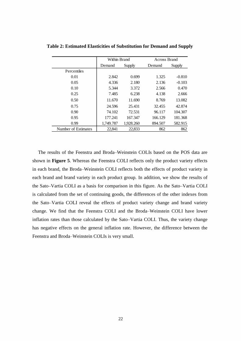
Table 2: Estimated Elasticities of Substitution for Demand and Supply
The results of the Feenstra and Broda–Weinstein COLIs based on the POS data are
shown in Figure 5. Whereas the Feenstra COLI reflects only the product variety effects
in each brand, the Broda–Weinstein COLI reflects both the effects of product variety in
each brand and brand variety in each product group. In addition, we show the results of
the Sato–Vartia COLI as a basis for comparison in this figure. As the Sato–Vartia COLI
is calculated from the set of continuing goods, the differences of the other indexes from
the Sato–Vartia COLI reveal the effects of product variety change and brand variety
change. We find that the Feenstra COLI and the Broda–Weinstein COLI have lower
inflation rates than those calculated by the Sato–Vartia COLI. Thus, the variety change
has negative effects on the general inflation rate. However, the difference between the
Feenstra and Broda–Weinstein COLIs is very small.
Demand Supply Demand Supply
Percentiles
0.01 2.842 0.699 1.325 -0.810
0.05 4.336 2.180 2.136 -0.103
0.10 5.344 3.372 2.566 0.470
0.25 7.485 6.238 4.138 2.666
0.50 11.670 11.690 8.769 13.082
0.75 24.596 25.431 32.455 42.874
0.90 74.102 72.531 96.117 104.307
0.95 177.241 167.347 166.129 181.368
0.99 1,749.787 1,928.260 894.507 582.915
Number of Estimates 22,841 22,833 862 862
Within Brand Across Brand

23
Figure 5: Sato–Vartia, Feenstra, and Broda–Weinstein COLIs and the Unit Value
Price Index
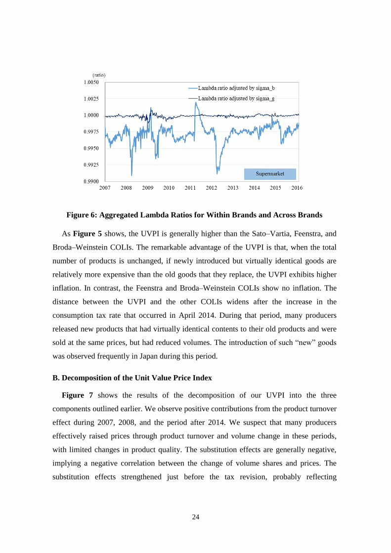
Figure 6 shows the aggregated within-brand and across-brand lambda ratios that are
adjusted by within-brand and across-brand substitution elasticities, respectively. Whereas
the within-brand lambda ratios adjusted by substitution elasticities are significantly lower
than unity, the across-brand lambda ratios adjusted by substitution elasticities have very
small fluctuations away from unity. Here, we use manufacturer information to identify
brands because of the difficulty of identifying within-brand variety in a manufacturer’s
products. Thus, the effects of brand variety changes are small.20
20 We use only the estimates of within-brand elasticities to calculate Feenstra’s COLI in which
brands are considered as product groups.
24
Figure 6: Aggregated Lambda Ratios for Within Brands and Across Brands
As Figure 5 shows, the UVPI is generally higher than the Sato–Vartia, Feenstra, and
Broda–Weinstein COLIs. The remarkable advantage of the UVPI is that, when the total
number of products is unchanged, if newly introduced but virtually identical goods are
relatively more expensive than the old goods that they replace, the UVPI exhibits higher
inflation. In contrast, the Feenstra and Broda–Weinstein COLIs show no inflation. The
distance between the UVPI and the other COLIs widens after the increase in the
consumption tax rate that occurred in April 2014. During that period, many producers
released new products that had virtually identical contents to their old products and were
sold at the same prices, but had reduced volumes. The introduction of such “new” goods
was observed frequently in Japan during this period.
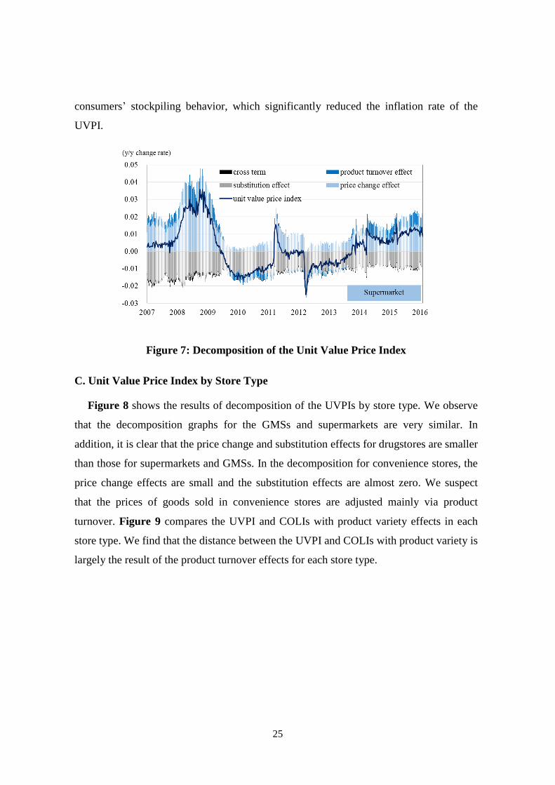
B. Decomposition of the Unit Value Price Index
Figure 7 shows the results of the decomposition of our UVPI into the three
components outlined earlier. We observe positive contributions from the product turnover
effect during 2007, 2008, and the period after 2014. We suspect that many producers
effectively raised prices through product turnover and volume change in these periods,
with limited changes in product quality. The substitution effects are generally negative,
implying a negative correlation between the change of volume shares and prices. The
substitution effects strengthened just before the tax revision, probably reflecting
25
consumers’ stockpiling behavior, which significantly reduced the inflation rate of the
UVPI.
Figure 7: Decomposition of the Unit Value Price Index
C. Unit Value Price Index by Store Type
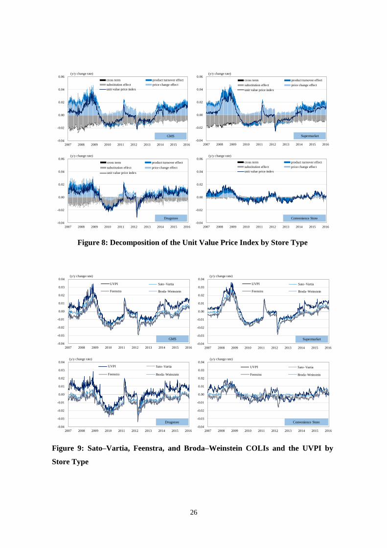
Figure 8 shows the results of decomposition of the UVPIs by store type. We observe
that the decomposition graphs for the GMSs and supermarkets are very similar. In
addition, it is clear that the price change and substitution effects for drugstores are smaller
than those for supermarkets and GMSs. In the decomposition for convenience stores, the
price change effects are small and the substitution effects are almost zero. We suspect
that the prices of goods sold in convenience stores are adjusted mainly via product
turnover. Figure 9 compares the UVPI and COLIs with product variety effects in each
store type. We find that the distance between the UVPI and COLIs with product variety is
largely the result of the product turnover effects for each store type.
26
Figure 8: Decomposition of the Unit Value Price Index by Store Type
Figure 9: Sato–Vartia, Feenstra, and Broda–Weinstein COLIs and the UVPI by
Store Type
-0.04
-0.02
0.00
0.02
0.04
0.06
2007 2008 2009 2010 2011 2012 2013 2014 2015 2016
cross term product turnover effect
substitution effect price change effect
unit value price index
GMS
(y/y change rate)
-0.04
-0.02
0.00
0.02
0.04
0.06
2007 2008 2009 2010 2011 2012 2013 2014 2015 2016
cross term product turnover effect
substitution effect price change effect
unit value price index
Supermarket
(y/y change rate)
-0.04
-0.02
0.00
0.02
0.04
0.06
2007 2008 2009 2010 2011 2012 2013 2014 2015 2016
cross term product turnover effect
substitution effect price change effect
unit value price index
Drugstore
(y/y change rate)
-0.04
-0.02
0.00
0.02
0.04
0.06
2007 2008 2009 2010 2011 2012 2013 2014 2015 2016
cross term product turnover effect
substitution effect price change effect
unit value price index
Convenience Store
(y/y change rate)
-0.04
-0.03
-0.02
-0.01
0.00
0.01
0.02
0.03
0.04
2007 2008 2009 2010 2011 2012 2013 2014 2015 2016
UVPI Sato–Vartia
Feenstra Broda–Weinstein
GMS
(y/y change rate)
-0.04
-0.03
-0.02
-0.01
0.00
0.01
0.02
0.03
0.04
2007 2008 2009 2010 2011 2012 2013 2014 2015 2016
UVPI Sato–Vartia
Feenstra Broda–Weinstein
Supermarket
(y/y change rate)
-0.04
-0.03
-0.02
-0.01
0.00
0.01
0.02
0.03
0.04
2007 2008 2009 2010 2011 2012 2013 2014 2015 2016
UVPI Sato–Vartia
Feenstra Broda–Weinstein
Drugstore
(y/y change rate)
-0.04
-0.03
-0.02
-0.01
0.00
0.01
0.02
0.03
0.04
2007 2008 2009 2010 2011 2012 2013 2014 2015 2016
UVPI Sato–Vartia
Feenstra Broda–Weinstein
Convenience Store
(y/y change rate)
27
VI. Quality Issues
As already pointed out, the turnover/new product effects are composed of two
different effects, changes in prices and changes in quality. It is virtually impossible to
quantify the contribution of the changes in quality within the turnover/new product
effects. However, by examining some cases of product turnover, we can gain some
insight into the relative importance of changes in quality.
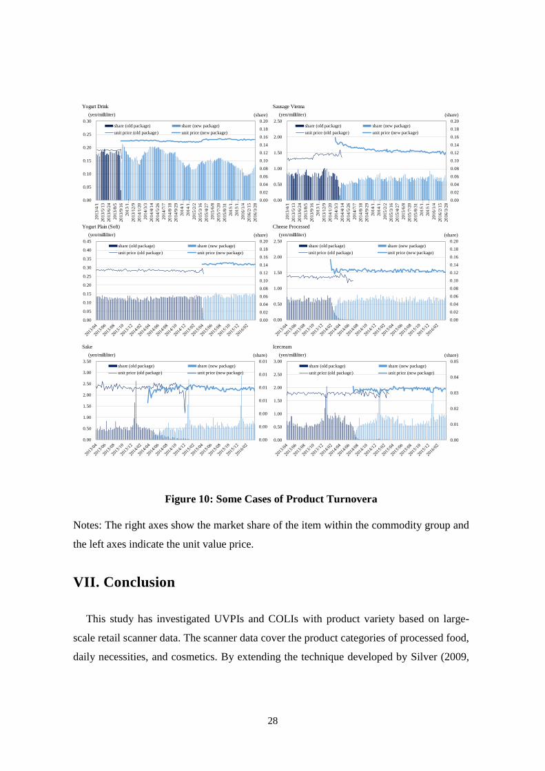
Between April 2014 and March 2015, the turnover/new product effect in supermarkets is
about 1.5 percentage points. About two-thirds of the increase came from changes in the
following six product categories: yogurt drinks, Vienna sausage, soft plain yogurt,
processed cheese, sake (rice wine), and ice cream. Figure 10 shows the movements in the
average price and sales volume of these product categories, based on the products with
the largest market shares for each of these six categories. Three products underwent
volume changes when the new products were introduced, without any statement about
quality improvements being made in their advertisements. For example, one processed
cheese product was reduced from eight slices of cheese to seven slices, with each slice
having the same volume and ingredients as the old product. Three commodities claimed
improvements in quality; for instance, a new yogurt drink that appeared in September
2013 came in a new container that was supposed to be easier to open, and it was claimed
that a new Vienna sausage introduced in early 2014 was tastier. Sake, Japanese rice wine,
is different from the other product categories. There was no major sake product that
contributed to the commodity-level turnover effects, implying that the increase in the
turnover/new product effects came from a number of different commodities with minor
market shares.
28
Figure 10: Some Cases of Product Turnovera
Notes: The right axes show the market share of the item within the commodity group and
the left axes indicate the unit value price.
VII. Conclusion
This study has investigated UVPIs and COLIs with product variety based on large-
scale retail scanner data. The scanner data cover the product categories of processed food,
daily necessities, and cosmetics. By extending the technique developed by Silver (2009,
Yogurt Drink Sausage Vienna
Yogurt Plain (Soft) Cheese Processed
Sake Icecream
0.00
0.02
0.04
0.06
0.08
0.10
0.12
0.14
0.16
0.18
0.20
0.00
0.05
0.10
0.15
0.20
0.25
0.30
20
13
/4/1
20
13
/5/1
3
20
13
/6/2
4
20
13
/8/5
20
13
/9/1
6
20
13
/1…
20
13
/12
/9
20
14
/1/2
0
20
14
/3/3
20
14
/4/1
4
20
14
/5/2
6
20
14
/7/7
20
14
/8/1
8
20
14
/9/2
9
20
14
/1…
20
14
/1…
20
15
/2/2
20
15
/3/1
6
20
15
/4/2
7
20
15
/6/8
20
15
/7/2
0
20
15
/8/3
1
20
15
/1…
20
15
/1…
20
16
/1/4
20
16
/2/1
5
20
16
/3/2
8
share (old package) share (new package)
unit price (old package) unit price (new package)
(yen/milliliter) (share)
0.00
0.02
0.04
0.06
0.08
0.10
0.12
0.14
0.16
0.18
0.20
0.00
0.50
1.00
1.50
2.00
2.50
20
13
/4/1
20
13
/5/1
3
20
13
/6/2
4
20
13
/8/5
20
13
/9/1
6
20
13
/1…
20
13
/12
/9
20
14
/1/2
0
20
14
/3/3
20
14
/4/1
4
20
14
/5/2
6
20
14
/7/7
20
14
/8/1
8
20
14
/9/2
9
20
14
/1…
20
14
/1…
20
15
/2/2
20
15
/3/1
6
20
15
/4/2
7
20
15
/6/8
20
15
/7/2
0
20
15
/8/3
1
20
15
/1…
20
15
/1…
20
16
/1/4
20
16
/2/1
5
20
16
/3/2
8
share (old package) share (new package)
unit price (old package) unit price (new package)
(yen/milliliter) (share)
0.00
0.02
0.04
0.06
0.08
0.10
0.12
0.14
0.16
0.18
0.20
0.00
0.05
0.10
0.15
0.20
0.25
0.30
0.35
0.40
0.45share (old package) share (new package)
unit price (old package) unit price (new package)
(yen/milliliter) (share)
0.00
0.02
0.04
0.06
0.08
0.10
0.12
0.14
0.16
0.18
0.20
0.00
0.50
1.00
1.50
2.00
2.50share (old package) share (new package)
unit price (old package) unit price (new package)
(yen/milliliter) (share)
0.00
0.01
0.02
0.03
0.04
0.05
0.00
0.50
1.00
1.50
2.00
2.50
3.00share (old package) share (new package)
unit price (old package) unit price (new package)
(yen/milliliter) (share)
0.00
0.00
0.00
0.01
0.01
0.01
0.01
0.00
0.50
1.00
1.50
2.00
2.50
3.00
3.50share (old package) share (new package)
unit price (old package) unit price (new package)
(yen/milliliter) (share)
29
2010) and Diewert and Von der Lippe (2010), we decomposed changes in the UVPI into
three contributions: (1) price change effects (Laspeyres price index), (2) substitution
effects, and (3) turnover/new goods effects. The aggregate UVPI shows a higher rate of
inflation than do COLIs, including the Sato–Vartia, Feenstra, and Broda–Weinstein
COLIs. Product turnover effects are generally positive, implying that new products are
priced higher than are disappearing or continuing goods. Substitution effects are
generally negative, implying a negative correlation between volume shares and prices.
Substitution effects strengthened just prior to Japan’s consumption tax revision in 2014,
probably reflecting consumers’ stockpiling behavior, which significantly reduced the
inflation rate of the UVPI. After the tax rate increased, the turnover/new product effects
increased by one percentage point, contributing to the increase in unit value prices.
Analyses at the store-type level revealed that the influence of the three effects on the
UVPI varied greatly across store types. We observed that the contributions of the price
change and substitution effects in drugstores are smaller than those in supermarkets and
GMSs. The decomposition of the UVPI for convenience stores shows an even smaller
price change effect, while the substitution effect is virtually zero.
There are a number of tasks relating to our work that remain a subject for future
research. The increasing share of new goods in total sales after Japan’s tax revision
implies that the introduction of new goods is used as an instrument for price adjustment
to a certain extent. The increase in the UVPI after the tax revision was caused largely by
the introduction of more highly priced new goods. If factors such as potential damage to
product brands prevent producers from changing prices, the introduction of new, slightly
different (e.g., reduced volume) goods could be a means of avoiding price increases while
reducing costs for producers. Microanalyses of price and product adjustments merit
further investigation.
The UVPI did not capture changes in product quality, such as taste or durability. In
general, the quality of processed foods and daily necessities is very difficult to measure.
The Statistics Bureau of Japan does not adjust for the quality of processed foods and
daily necessities, except for volume (changes in grams or milliliters), when constructing
30
its CPI. As there is scarce information about the characteristics of processed food and
daily necessities, except for volume, it is difficult to employ a hedonic approach. As
Section 6 discusses, we suspect the contribution of changes in quality is minor in our
UVPIs. However, more detailed categorical-level investigations are needed to address the
quality issue further.
Other tasks remaining for future research include analyses of: (1) the effects of the tax
rate on the cycle of products introduced just before the tax reform; (2) other possible
measures for the COLI, including the multilateral chained index proposed by De Haan
and Van der Grient (2011); and (3) the impact on commodity prices of the large
depreciation in the Japanese yen in 2012.21
21 Recent works including Shioji (2015) and Hara et al. (2015) show that the exchange rate
pass-through into the Japanese price index increased after 2010.
31
Appendix A
A.1. Rate of Inflation of the Unit Value Price Index
The inflation rate of the UVPI, 𝜋𝑡𝑈(≡
𝑃𝑡𝑈−𝑃𝑡−𝑦
𝑈
𝑃𝑡−𝑦𝑈 ), can be written as follows:22
𝜋𝑡𝑈 = (
𝑃𝑡−𝑦𝑈𝐶
𝑃𝑡−𝑦𝑈 )
𝑤𝑡𝐶𝑃𝑡
𝑈𝐶−𝑤𝑡−𝑦𝐶 𝑃𝑡−𝑦
𝑈𝐶
𝑃𝑡−𝑦𝑈𝐶 + (
𝑃𝑡−𝑦𝑈𝑂
𝑃𝑡−𝑦𝑈 )
𝑤𝑡𝑁𝑃𝑡
𝑈𝑁−𝑤𝑡−𝑦𝑂 𝑃𝑡−𝑦
𝑈𝑂
𝑃𝑡−𝑦𝑂 .
We rewrite this equation as:
𝜋𝑡𝑈 = (
𝑃𝑡−𝑦𝑈𝐶
𝑃𝑡−𝑦𝑈 )𝑤𝑡−𝑦
𝐶 �̂�𝑡𝑈𝐶 + (
𝑃𝑡−𝑦𝑈𝑂
𝑃𝑡−𝑦𝑈 )𝑤𝑡−𝑦
𝑂 �̂�𝑡𝑈𝑇 ,
where �̂�𝑡𝑈𝐶 ≡
(𝑤𝑡𝐶 𝑤𝑡−𝑦
𝐶⁄ )𝑃𝑡𝑈𝐶−𝑃𝑡−𝑦
𝑈𝐶
𝑃𝑡−𝑦UC and �̂�𝑡
𝑈𝑇 ≡(𝑤𝑡
𝑁 𝑤𝑡−𝑦𝑂⁄ )𝑃𝑡
𝑈𝑁−𝑃𝑡−𝑦𝑈𝑂
𝑃𝑡−𝑦𝑈𝑂 .
A.2. Price Change Effects and Substitution Effects
We define the Laspeyres price index of the continuing goods (𝜋𝑡𝐿𝐶) as follows:23
𝜋𝑡𝐿𝐶 =
∑ [𝑞𝑡−𝑦𝑖
∑ 𝑞𝑡−𝑦𝑖
𝑖∈𝑔𝑡,𝑡−𝑦
×𝑝𝑡𝑖]𝑖∈𝑔𝑡,𝑡−𝑦 − ∑ [
𝑞𝑡−𝑦𝑖
∑ 𝑞𝑡−𝑦𝑖
𝑖∈𝑔𝑡,𝑡−𝑦
×𝑝𝑡−𝑦𝑖 ]𝑖∈𝐶𝑡
∑ [𝑞𝑡−𝑦𝑖
∑ 𝑞𝑡−𝑦𝑖
𝑖∈𝑔𝑡,𝑡−𝑦
×𝑝𝑡−𝑦𝑖 ]𝑖∈𝐶𝑡
=∑ [𝑞𝑡−𝑦
𝑖 𝑝𝑡𝑖]𝑖∈𝑔𝑡,𝑡−𝑦
∑ [𝑞𝑡−𝑦𝑖 𝑝𝑡−𝑦
𝑖 ]𝑖∈𝑔𝑡,𝑡−𝑦
− 1.
As 𝜋𝑡𝐿𝐶 captures the effects of price changes of the continuing goods, we refer to it as the
price change effects.
The substitution effect of continuing goods (𝜙t𝑈𝐶) is defined as:
22 In the appendix, we omit the indicator of product category 𝑔. Thus, here, we denote 𝑃𝑡𝑈 as
𝑃𝑡𝑈(𝑔).
23 In the appendix, 𝑝𝑡𝑖 denotes 𝑝𝑡
𝑖/𝑣𝑖 in the main text and 𝑞𝑡−𝑦𝑖 denotes 𝑣𝑖𝑞𝑡−𝑦
𝑖 in the main text.

32
𝜙t𝑈𝐶 ≡
𝑃𝑡𝑈𝐶 − �̈�𝑡
𝑈𝐶
𝑃𝑡UC
,
where �̈�𝑡𝑈𝐶 = ∑ [
𝑞𝑡−𝑦𝑖
∑ 𝑞𝑡−𝑦𝑖
𝑖∈𝑔𝑡,𝑡−𝑦
×𝑝𝑡𝑖]𝑖∈𝑔𝑡,𝑡−𝑦 .
Diewert and Von der Lippe (2010) define covariance such that:
Cov(𝑥, 𝑦) =1
𝑇∑ (𝑥𝑖 − 𝑥
∗)(𝑦𝑖 − 𝑦∗)𝑖 =
1
𝑇∑ (𝑥𝑖)(𝑦𝑖 − 𝑦
∗)𝑖 ,
where
𝑠𝑡𝑖 =
𝑞𝑡𝑖
∑ 𝑞𝑡𝑖
𝑖∈𝑔𝑡,𝑡−𝑦
, 𝑝t = [𝑝𝑡1, 𝑝𝑡
2, … , 𝑝𝑡𝑇𝑡], and 𝑠𝑡 = [𝑠𝑡
1, 𝑠𝑡2, … , 𝑠𝑡
𝑇𝑡],
where 𝑇𝑡: #(𝛩𝑡) is the number of products sold at time 𝑡.
The substitution effects (𝜙𝑡𝐶) can be transformed as follows:
𝜙𝑡𝑈𝐶 ≡
𝑃𝑡𝑈𝐶 − �̈�𝑡
𝑈𝐶
𝑃𝑡𝑈𝐶 =
∑ 𝑝𝑡𝑖 [
𝑞𝑡𝑖
∑ 𝑞𝑡𝑖
𝑖∈𝑔𝑡,𝑡−𝑦
−𝑞𝑡−𝑦𝑖
∑ 𝑞𝑡−𝑦𝑖
𝑖∈𝑔𝑡,𝑡−𝑦
]𝑖∈𝑔𝑡,𝑡−𝑦
∑ [𝑞𝑡𝑖
∑ 𝑞𝑡𝑖
𝑖∈𝑔𝑡,𝑡−𝑦
×𝑝𝑡𝑖]𝑖∈𝐶𝑡
=∑ 𝑝𝑡
𝑖[𝑠𝑡𝑖 − 𝑠𝑡−𝑦
𝑖 ]𝑖∈𝑔𝑡,𝑡−𝑦
∑ [𝑞𝑡𝑖
∑ 𝑞𝑡𝑖
𝑖∈𝑔𝑡,𝑡−𝑦
×𝑝𝑡𝑖]𝑖∈𝑔𝑡,𝑡−𝑦
.
Because 𝑠𝑡𝑖 and 𝑠𝑡−𝑦
𝑖 are the volume shares of good i in times t and t−y, respectively, their
averages are the same. That is, ∑ [𝑠𝑡𝑖 − 𝑠𝑡−𝑦
𝑖 ]𝑖∈𝐶𝑡 = 0.
Thus, we obtain:
∑𝑝𝑡𝑖[𝑠𝑡
𝑖 − 𝑠𝑡−𝑦𝑖 ]
𝑖∈𝑐𝑡
= 𝑇𝑡Cov(𝑝𝑡, 𝑠𝑡 − 𝑠𝑡−𝑦).
Therefore, the substitution effects can be written by the following covariance:
33
𝜙𝑡𝑈𝐶 =
𝑇𝑡Cov(𝑝𝑡, 𝑠𝑡 − 𝑠𝑡−𝑦)
𝑃𝑡𝑈𝐶 .
The RHS of the above equation is equivalent to the formula derived by Diewert and Von
der Lippe (2010). The interpretation of the covariance term is straightforward. If the price
of good i were to exceed the average price, its volume share would be expected to
decline. This substitution effect captures the degree of the negative correlation.
A.3. Decomposition of �̂�𝒕𝑪
To interpret the term with �̂�𝑡𝑐, we introduce variable �̃�𝑡
C, as follows:
�̃�𝑡𝑈𝐶 ≡ �̂�𝑡
𝑈𝐶 − 𝜋𝑡𝐿𝐶
= (𝑤𝑡𝐶 𝑤𝑡−𝑦
𝐶⁄ − 1)𝑃𝑡𝑈𝐶
𝑃𝑡−𝑦𝑈𝐶 +
𝑃𝑡𝑈𝐶 − �̈�𝑡
𝑈𝐶
𝑃𝑡𝑈𝐶
𝑃𝑡𝑈𝐶
𝑃𝑡−𝑦𝑈𝐶
= (𝑤𝑡𝐶 𝑤𝑡−𝑦
𝐶⁄ − 1)(1 + 𝜋𝑡𝑈𝐶) + 𝜙𝑡
𝐶(1 + 𝜋𝑡𝑈𝐶),
where 𝜋𝑡𝑈𝐶 ≡
𝑃𝑡𝑈𝐶−𝑃𝑡−𝑦
𝑈𝐶
𝑃𝑡−𝑦𝑈𝐶 .
Therefore, �̂�𝑡𝑈𝐶 can be expressed as:
�̂�𝑡𝑈𝐶 = 𝜋𝑡
𝐿𝐶 + 𝜙𝑡𝑈𝐶 + (𝑤𝑡
𝐶 𝑤𝑡−𝑦𝐶⁄ − 1) + [(𝑤𝑡
𝐶 𝑤𝑡−𝑦𝐶⁄ − 1)𝜋𝑡
𝑈𝐶 + 𝜙𝑡𝑈𝐶𝜋𝑡
𝑈𝐶].
�̂�𝑡𝑈𝐶 can be decomposed into four effects: (1) the price change effects of continuing
goods, 𝜋𝑡𝐿𝐶; (2) the substitution effects within continuing goods, 𝜙𝑡
𝑈𝐶; (3) the changes in
the weights of continuing goods between periods t and t−y, (𝑤𝑡𝐶 𝑤𝑡−𝑦
𝐶⁄ − 1); and (4) the
cross-terms.
A.4. Decomposition of �̂�𝒕𝑼𝑻
�̂�𝑡𝑈𝑇 can be decomposed into three effects: (1) the changes in the weights of new and
disappearing goods, (𝑤𝑡𝑁 𝑤𝑡−𝑦
𝑂⁄ − 1); (2) the price differential between new and
disappearing goods, 𝜋𝑡𝑁𝑂; and (3) the cross-term, as follows:
34
�̂�𝑡𝑈𝑇 = (𝑤𝑡
𝑁 𝑤𝑡−𝑦𝑂⁄ − 1)+𝜋𝑡
𝑁𝑂 + (𝑤𝑡𝑁 𝑤𝑡−𝑦
𝑂⁄ − 1)𝜋𝑡𝑁𝑂 ,
where 𝜋𝑡𝑁𝑂 ≡
𝑃𝑡𝑈𝑁−𝑃𝑡−𝑦
𝑈𝑂
𝑃𝑡−𝑦𝑈𝑂 .
A.5. Unit Value Price Decomposition
𝜋𝑡𝑈 can be expressed as:
𝜋𝑡𝑈 = (
𝑃𝑡−𝑦𝑈𝐶
𝑃𝑡−𝑦𝑈 )𝑤𝑡−𝑦
𝐶 𝜋𝑡𝐿𝐶 + (
𝑃𝑡−𝑦𝑈𝐶
𝑃𝑡−𝑦𝑈 )𝑤𝑡−𝑦
𝐶 𝜙𝑡𝑈𝐶 + (
𝑃𝑡−𝑦𝑈𝑂
𝑃𝑡−𝑦𝑈 )𝑤𝑡−𝑦
𝑂 𝜋𝑡𝑁𝑂
+ (𝑃𝑡−𝑦𝐶
𝑃𝑡−𝑦𝛩 ) (𝑤𝑡
𝐶 − 𝑤𝑡−𝑦𝐶 )𝜋𝑡
𝑈𝐶 + (𝑃𝑡−𝑦𝑈𝑂
𝑃𝑡−𝑦𝑈 ) (𝑤𝑡
𝑁 − 𝑤𝑡−𝑦𝑂 )𝜋𝑡
𝑁𝑂
+ (𝑃𝑡−𝑦𝑈𝑂 − 𝑃𝑡−𝑦
𝑈𝐶
𝑃𝑡−𝑦𝑈 ) (𝑤𝑡
𝑁 − 𝑤𝑡−𝑦𝑂 ) + (
𝑃𝑡−𝑦𝑈𝐶
𝑃𝑡−𝑦𝑈 )𝑤𝑡−𝑦
𝐶 𝜙𝑡𝑈𝐶𝜋𝑡
𝑈𝐶 .
The third, fourth, fifth, and sixth terms on the RHS of the above equation can be
simplified significantly, as follows:
(𝑃𝑡−𝑦𝑈𝑂
𝑃𝑡−𝑦𝑈 )𝑤𝑡−𝑦
𝑂 𝜋𝑡𝑁𝑂 + (
𝑃𝑡−𝑦𝐶
𝑃𝑡−𝑦𝛩 ) (𝑤𝑡
𝐶 − 𝑤𝑡−𝑦𝐶 )𝜋𝑡
𝑈𝐶 + (𝑃𝑡−𝑦𝑈𝑂
𝑃𝑡−𝑦𝑈 ) (𝑤𝑡
𝑁 − 𝑤𝑡−𝑦𝑂 )𝜋𝑡
𝑁𝑂
+ (𝑃𝑡−𝑦𝑈𝑂 − 𝑃𝑡−𝑦
𝑈𝐶
𝑃𝑡−𝑦𝑈 ) (𝑤𝑡
𝑁 − 𝑤𝑡−𝑦𝑂 )
=𝑤𝑡−𝑦𝑂 (𝑃𝑡
𝑈𝐶 − 𝑃𝑡−𝑦𝑈𝑂 ) + 𝑤𝑡
𝑁(𝑃𝑡𝑈𝑁 − 𝑃𝑡
𝑈𝐶)
𝑃𝑡−𝑦𝑈 .
Note that 𝑤𝑡𝐶 − 𝑤𝑡−𝑦
𝐶 = 1 − 𝑤𝑡𝑁 − (1 − 𝑤𝑡−𝑦
𝑂 ) = −(𝑤𝑡𝑁 − 𝑤𝑡−𝑦
𝑂 ).
Thus, we obtain:
𝜋𝑡𝑈 = (
𝑃𝑡−𝑦𝑈𝐶
𝑃𝑡−𝑦𝑈 )𝑤𝑡−𝑦
𝐶 𝜋𝑡𝐿𝐶 + (
𝑃𝑡−𝑦𝑈𝐶
𝑃𝑡−𝑦𝑈 )𝑤𝑡−𝑦
𝐶 𝜙𝑡𝑈𝐶 +
𝑤𝑡−𝑦𝑂 (𝑃𝑡
𝑈𝐶 − 𝑃𝑡−𝑦𝑈𝑂 ) + 𝑤𝑡
𝑁(𝑃𝑡𝑈𝑁 − 𝑃𝑡
𝑈𝐶)
𝑃𝑡−𝑦𝑈
+ (𝑃𝑡−𝑦𝑈𝐶
𝑃𝑡−𝑦𝑈 )𝑤𝑡−𝑦
𝐶 𝜙𝑡𝑈𝐶𝜋𝑡
𝑈𝐶 .

35
Appendix B
Feenstra (1994) estimates the substitution elasticity for demand and supply
simultaneously based on continuing goods transaction data. In Subsection 2.1, we assume
composite consumption, as follows:
𝐶𝑡𝑔= (∑𝛼𝑖(𝑞𝑡
𝑖)
𝜎𝑔−1
𝜎𝑔
𝑖∈𝑔𝑡
)
𝜎𝑔𝜎𝑔−1
.
Then, the consumption share of product 𝑖 in category 𝑔 is given by the following
expression:
𝑤𝑡𝑖 = (
𝐸𝑡
𝐶𝑡𝑔)𝜎𝑔−1
𝑎𝑖
𝜎𝑔𝑝𝑡𝑖1−𝜎𝑔,
where 𝑤𝑡𝑖 = 𝑝𝑡
𝑖𝑞𝑡𝑖/(∑ 𝑝𝑡
𝑖𝑞𝑡𝑖
𝑖∈𝑔𝑡,𝑡−𝑦 ).
Taking the log in the first difference of this expression yields:
∆ln𝑤𝑡𝑖 = 𝛾𝑡 − (𝜎𝑔 − 1)∆ ln 𝑝𝑡
𝑖 + 휀𝑡𝑖, (A1)
where 𝛾𝑡=(𝜎𝑔 − 1)∆ln (𝐸𝑡/𝐶𝑡𝑔) and 휀𝑡
𝑖 = 𝜎𝑔ln 𝑎𝑖.
The supply curve of product 𝑖 in category 𝑔 is specified in the following log difference
form:
∆ ln 𝑝𝑡𝑖 = ωgΔ ln 𝑞𝑡
𝑖 + 𝜉𝑡𝑖, (A2)
where ωg is the inverse supply elasticity and 𝜉𝑡𝑖 is a supply shock, which is assumed
independent to 휀𝑡𝑖. From equations (A1) and (A2), we obtain the following expression:
∆ ln 𝑝𝑡𝑖 = 𝜓𝑡 +
𝜌
𝜎𝑔 − 1휀𝑡𝑖 + 𝛿𝑡
𝑖, (A3)
where 𝜓𝑡 =𝜔𝑔
1+𝜎𝑔𝜔𝑔 (𝛾𝑡 + ∆ln 𝐸𝑡) , 𝛿𝑡
𝑖 = 𝜉𝑡𝑖/(1 + 𝜎𝑔𝜔𝑔) , and 𝜌 = 𝜔𝑔(𝜎𝑔 − 1)/(1 +
𝜎𝑔𝜔𝑔).
36
If we were to subtract the same functions for product 𝑘 in category 𝑔 from equations
(A1) and (A3), we could eliminate 𝛾𝑡 and 𝜓𝑡 and obtain the following expression:
휀�̃�𝑖 = (∆ln𝑤𝑡
𝑖 − ∆ln𝑤𝑡𝑘) + (𝜎𝑔 − 1)(∆ln 𝑝𝑡
𝑖 − ∆ln 𝑝𝑡𝑘)
𝛿𝑡𝑖 = (1 − 𝜌)(∆ln𝑝𝑡
𝑖 − ∆ln 𝑝𝑡𝑘) − (
𝜌
𝜎𝑔−1) (∆ln𝑤𝑡
𝑖 − ∆ln𝑤𝑡𝑘),
where 휀�̃�𝑖 = 휀𝑡
𝑖 − 휀𝑡𝑘 and 𝛿𝑡
𝑖 = 𝛿𝑡𝑖 − 𝛿𝑡
𝑘. Multiplying these two equations and dividing the
result by (1 − 𝜌)(𝜎𝑔 − 1), we obtain the following equation:
𝑌𝑡𝑖 = 𝜃1𝑋𝑡
𝑖 + 𝜃2𝑍𝑡𝑖 + 𝑢𝑡
𝑖 , (A4)
where
𝑌𝑡𝑖 = (∆ln 𝑝𝑡
𝑖 − ∆ln 𝑝𝑡𝑘)2, 𝑋𝑡
𝑖 = (∆ln𝑤𝑡𝑖 − ∆ln𝑤𝑡
𝑘)2,
𝑍𝑡𝑖 = (∆ln𝑤𝑡
𝑖 − ∆ln𝑤𝑡𝑘)(∆ln 𝑝𝑡
𝑖 − ∆ln 𝑝𝑡𝑘),
𝑢𝑡𝑖 =
휀�̃�𝑖𝛿𝑡𝑖
(1 − 𝜌)(𝜎𝑔 − 1), 𝜃1 =
𝜌
(1 − 𝜌)(𝜎𝑔 − 1)2 , 𝜃2 =
(2𝜌 − 1)
(1 − 𝜌)(𝜎𝑔 − 1).
To obtain consistent estimators, we take the average of equation (A4) for all 𝑡:
�̅�𝑖 = 𝜃1�̅�𝑖 + 𝜃2�̅�
𝑖 + �̅�𝑖 . (A5)
From the assumption of demand and supply shocks, E(�̅�𝑖) = 0. We estimate 𝜎𝑔 and 𝜔𝑔
using equation (A5) by GMM.
When we perform the within-brand estimation, we denote the individual price and share
in the brand as 𝑝𝑡𝑖 and 𝑤𝑡
𝑖, respectively. When we estimate the within-brand estimation,
we adopt 𝑃𝐼𝑆𝑉(𝑝𝑡, 𝑝𝑡−𝑦 , 𝑏𝑡,𝑡−𝑦) (𝜆𝑏𝑡cr
𝜆𝑏𝑡bs)
1
𝜎𝑏−1 and
𝑤𝑡𝑏 =
∑ 𝑝𝑡𝑖𝑞𝑡𝑖
𝑖∈𝑏𝑡,𝑡−𝑦
∑ ∑ 𝑝𝑡𝑖𝑞𝑡𝑖
𝑖∈𝑏𝑡,𝑡−𝑦𝑏∈𝑔 as 𝑝𝑡
𝑖 and 𝑤𝑡𝑖, respectively, in this estimation procedure.
37
References
Balk, B.M. 2000. On Curing the CPI’s Substitution and New Goods Bias. Research
Paper No. 0005, Statistics Netherlands: Voorburg.
Bernard, A.B., J.S. Redding, and P.K. Schott. 2010. “Multiple-product firms and
product switching,” American Economic Review 100(1): 70–97.
Bilbiie, F.O., F. Ghironi, and M.J. Melitz. 2012. “Endogenous entry, product variety,
and business cycles,” Journal of Political Economy 120(2): 304–345.
Bils, M. 2009. “Do higher prices for new goods reflect quality growth or inflation?”
Quarterly Journal of Economics 124(2): 637–675.
Broda, C., and D.E. Weinstein. 2010. “Product creation and destruction: evidence
and price implications,” American Economic Review 100: 691–723.
De Haan, J., and H.A. van der Grient. 2011. “Eliminating chain drift in price indexes
based on scanner data,” Journal of Econometrics 161(1): 36–46.
Diewert, W.E., and P. von der Lippe. 2010. “Notes on unit value index bias,”
Journal of Economics and Statistics 230(6): 690–708.
Feenstra, R.C. 1994. “New product varieties and the measurement of international
prices,” American Economic Review 84(1): 157–177.
Feenstra, R.C., and M.D. Shapiro. 2003. “High-frequency substitution and the
measurement of price indexes,” in Feenstra, R.C., and M.D. Shapiro (eds.) Scanner
Data and Price Indexes. The University of Chicago Press: Chicago, 123–150.
Fisher, I. 1922. The Making of Index Numbers, Houghton Mifflin: Boston.
Hamano, M. 2013. “On business cycles of product variety and quality,” CREA
Discussion Paper Series 13–21, Center for Research in Economic Analysis,
University of Luxembourg.
Hara, N., K. Hiraki, and Y. Ichise, 2015. “Changing exchange rate pass-through in
Japan: does it indicate changing pricing behavior? ” Bank of Japan Working Paper
Series 15-E-4, Bank of Japan.
International Labor Organization, Organisation for Economic Co-operation and
Development, Statistical Office of the European Communities, United Nations, and

38
World Bank. 2004. Consumer Price Index Manual: Theory and Practice.
International Labour Office: Geneva.
Klenow, P.J. 2003. “Measuring consumption growth: the impact of new and better
products,” Federal Reserve Bank of Minneapolis Quarterly Review 27(1): 10–23.
Melser, D., and I.A. Syed. 2013. “Prices over the product life cycle: implications for
quality-adjustment and the measurement of inflation,” UNSW Australian School of
Business Research Paper No. 2013–26, UNSW: Sydney.
Sato, K. 1976. “The ideal log-change index number,” Review of Economics and
Statistics 85(4): 777–792.
Shioji, E. 2015. “Time varying pass-through: will the yen depreciation help Japan hit
the inflation target?” Journal of the Japanese and International Economies, 37: 43–
58.
Silver, M. 2009. “Unit value indices,” in M. Silver (ed.) Export and Import Price
Index Manual, IMF: Washington DC, Chapter 2.
Silver, M. 2010. “The wrongs and rights of unit value indices,” Review of Income
and Wealth 56: 206–223.
Vartia, Y. 1976. “Ideal log-change index numbers,” Scandinavian Journal of
Statistics 3(3): 121–126.


