University of Wisconsin MilwaukeeUWM Digital Commons
Theses and Dissertations
May 2014
Re-Examining an Air Mass-Based Approach toDetecting Structural Climate Change, 1948-2011Joseph James LarsenUniversity of Wisconsin-Milwaukee
Follow this and additional works at: https://dc.uwm.edu/etdPart of the Climate Commons, Geography Commons, and the Meteorology Commons
This Thesis is brought to you for free and open access by UWM Digital Commons. It has been accepted for inclusion in Theses and Dissertations by anauthorized administrator of UWM Digital Commons. For more information, please contact [email protected].
Recommended CitationLarsen, Joseph James, "Re-Examining an Air Mass-Based Approach to Detecting Structural Climate Change, 1948-2011" (2014).Theses and Dissertations. 410.https://dc.uwm.edu/etd/410
RE-EXAMINING AN AIR MASS-BASED APPROACH TO DETECTING
STRUCTURAL CLIMATE CHANGE, 1948-2011
by
Joseph Larsen
A Thesis Submitted in
Partial Fulfillment of the
Requirements for the Degree of
Master of Science
in Geography
at
The University of Wisconsin-Milwaukee
May 2014
ii
ABSTRACT
RE-EXAMINING AN AIR MASS-BASED APPROACH TO
DETECTING STRUCTURAL CLIMATE CHANGE, 1948-2011
by
Joseph Larsen
The University of Wisconsin-Milwaukee, 2014
Under the Supervision of Professor Mark D. Schwartz
Air mass-based approaches to observing changes in climate can have considerable value
beyond simple trends of temperature and moisture, providing more thorough
understanding of structural climate patterns. Few methodologies have adequately
characterized recent air mass modification, however. This research seeks to update and
improve upon the methods of a prior study, providing new data from 1948-2011, as well
as more rigorous statistical analyses. Air mass types were created, and monthly averages
of temperature, dewpoint, and relative frequency were calculated for each of the air
masses in all four seasons; then the time series were submitted to regression analysis. The
results of this re-analysis show an increase in warm air masses at the expense of cool air
masses coinciding with the patterns of surface temperature and air mass warming seen in
other recent studies. Some changes in the behavior of these air masses were noted,
however, along with new variations in the character of others. These air mass trends have
conceivable ties to prior general circulation patterns. Assuming that previous patterns
have continued a possible increase in troughs, with a simultaneous decrease in ridges, in
the western United States may be occurring, while new patterns of air mass source region

iii
modification and air mass mixing could also exist. Systematic warming of air masses also
has conceivable, though rather modest relationships with large scale circulation patterns,
including positive phases of the Arctic Oscillation (AO) and North Atlantic Oscillation
(NAO), as well as contraction of the circumpolar vortex.
Keywords: climate change, synoptic climatology, air mass, mid-tropospheric (500-hPa)
circulation, integrated method, piecewise regression

iv
© Copyright by Joseph Larsen 2014
All Rights Reserved

v
TABLE OF CONTENTS
Abstract ............................................................................................................................ii
Copyright .........................................................................................................................iv
List of Figures ..................................................................................................................vii
List of Tables ...................................................................................................................x
Acknowledgements ..........................................................................................................xi
Chapter I: Introduction .....................................................................................................1
Chapter II: Review of Literature ......................................................................................4
A. Synoptic Methods as Alternatives to Empirical Assessments of Climate
Change ............................................................................................................4
B. Synoptic Classification Techniques and Assessment of Climate Change ......7
i. Manual Methods ...................................................................................9
ii. Automated Methods.............................................................................11
iii. Integrated Methods .............................................................................14
Chapter III: Study Objectives and Research Questions ...................................................21
Chapter IV: Study Area and Datasets ..............................................................................25
A. Study Area Selection .......................................................................................25
B. Datasets: Temperature—Dewpoint, Air Mass Types, Circulation
Linkages ..........................................................................................................26
Chapter V: Methodology .................................................................................................28
A. Baseline Temperature-Dewpoint Trend Analysis ...........................................28
B. Application of Integrated Classification Methodology ...................................29
C. Air Mass Characteristic Trend Analysis .........................................................31
D. Examination of Sub-Regional Modifications .................................................32

vi
E. Piecewise Linear Regression with Estimated Breakpoints .............................34
F. General Circulation Linkages ..........................................................................37
Chapter VI: Results ..........................................................................................................38
A. Seasonal Air Mass Frequency .........................................................................38
i. January ..................................................................................................38
ii. April .....................................................................................................39
iii. July......................................................................................................40
iv. October................................................................................................41
B. Air Mass Characteristic Trends .......................................................................55
i. January ..................................................................................................55
ii. April .....................................................................................................56
iii. July......................................................................................................58
iv. October................................................................................................60
Chapter VII: Discussion, Conclusions, and Recommendations ......................................74
A. Discussion .......................................................................................................74
B. Conclusions and Recommendations................................................................83
Literature Cited ................................................................................................................86

vii
LIST OF FIGURES
Figure 1: The North Central United States (NCUS) ........................................................26
Figure 2: Air mass criteria in January, April, July, and October for the
North Central United States .............................................................................................31
Figure 3: Relative frequency (in percent) of Continental air masses, January
1948-2011 ........................................................................................................................44
Figure 4: Relative Frequency (in percent) of Pacific air masses, January 1948-
2011..................................................................................................................................44
Figure 5: Relative frequency (in percent) of Dilute Tropical air masses, January
1948-2011 ........................................................................................................................45
Figure 6: Relative frequency (in percent) of Tropical air masses, January 1948-
2011..................................................................................................................................45
Figure 7: Relative frequency (in percent) of Unclassed air masses, January 1948-
2011..................................................................................................................................46
Figure 8: Relative frequency (in percent) of Continental air masses, April 1948-
2011..................................................................................................................................46
Figure 9: Relative frequency (in percent) of Pacific air masses, April 1948-
2011..................................................................................................................................47
Figure 10: Relative frequency (in percent) of Dry Tropical air masses, April
1948-2011 ........................................................................................................................47
Figure 11: Relative frequency (in percent) of Dilute Tropical air masses, April
1948-2011 ........................................................................................................................48
Figure 12: Relative frequency (in percent) of Tropical air masses, April 1948-
2011..................................................................................................................................48
Figure 13: Relative frequency (in percent) of Unclassed air masses, April 1948-
2011..................................................................................................................................49
Figure 14: Relative frequency (in percent) of Polar air masses, July 1948-2011 ............49
Figure 15: Relative frequency (in percent) of Dry Tropical air masses, July
1948-2011 ........................................................................................................................50

viii
Figure 16: Relative frequency (in percent) of Tropical air masses, July 1948-
2011..................................................................................................................................50
Figure 17: Relative frequency (in percent) of Unclassed air masses, July 1948-
2011..................................................................................................................................51
Figure 18: Relative frequency (in percent) of Continental air masses, October
1948-2011 ........................................................................................................................51
Figure 19: Relative frequency (in percent) of Pacific air masses, October 1948-
2011..................................................................................................................................52
Figure 20: Relative frequency (in percent) of Dry Tropical air masses, October
1948-2011 ........................................................................................................................52
Figure 21: Relative frequency (in percent) of Dilute Tropical air masses,
October 1948-2011 ..........................................................................................................53
Figure 22: Relative frequency (in percent) of Tropical air masses, October 1948-
2011..................................................................................................................................53
Figure 23: Relative frequency (in percent) of Unclassed air masses, October
1948-2011 ........................................................................................................................54
Figure 24: Five station mean January Pacific dewpoint temperature departures
from 1981-2010 normals..................................................................................................68
Figure 25: Six station mean April Continental relative frequency departures
from 1981-2010 normals..................................................................................................69
Figure 26: Five station mean April Dry Tropical relative frequency departures
from 1981-2010 normals..................................................................................................69
Figure 27: Ten station mean April Unclassed relative frequency departures
from 1981-2010 normals..................................................................................................70
Figure 28: Six station mean April Pacific dewpoint temperature departures
from 1981-2010 normals..................................................................................................70
Figure 29: Ten station mean July Polar relative frequency departures from
1981-2010 normals ..........................................................................................................71
Figure 30: Eight station mean July Tropical relative frequency departures
from 1981-2010 normals..................................................................................................71

ix
Figure 31: Five station mean July Unclassed relative frequency departures
from 1981-2010 normals..................................................................................................72
Figure 32: Five station mean July Dry Tropical temperature departures from
1981-2010 normals ..........................................................................................................72
Figure 33: Eleven station mean October Pacific dewpoint temperature
departures from 1981-2010 normals ................................................................................73
x
LIST OF TABLES
Table 1: Diagnostics for selection of major air masses ...................................................34
Table 2: January (winter) air mass percentages by station, 1948-2011 ...........................42
Table 3: April (spring) air mass percentages by station, 1948-2011 ...............................42
Table 4: July (summer) air mass percentages by station, 1948-2011 ..............................43
Table 5: October (autumn) air mass percentages by station, 1948-2011 .........................43
Table 6: Baseline temperature-dewpoint trends ..............................................................62
Table 7: Major air mass frequency trends........................................................................63
Table 8: Major air mass temperature-dewpoint trends ....................................................64
Table 9: Minor air mass frequency trends .......................................................................65
Table 10a: Minor air mass temperature-dewpoint trends ................................................66
Table 10b: Minor air mass temperature-dewpoint trends (cont.) ....................................67

xi
ACKNOWLEDGEMENTS
Special thanks to my advisor, Dist. Prof. Mark D. Schwartz for his insight, guidance, and
patience throughout the process of this research. Thanks to my committee members Dr.
Glen Fredlund and Dr. Woonsup Choi for their feedback and recommendations. I would
also like to thank Isaac Park, who provided considerable advice on the methods used in
this work. Finally, I would like to thank my fellow graduate students, friends, and family
for their love and support.

1
Chapter I: Introduction
Air masses have been studied, classified, and utilized for climatic research in a
number of ways. Conceptualized as large, relatively uniform regions of the atmosphere,
they were first proposed as a weather prediction aid, due to their convenience in
analyzing, describing, and understanding the variability of daily weather patterns
(Willett, 1933; Showalter, 1939; Schwartz, 1982). The grouping of meteorological
features such as air masses is also necessary in order to understand how different
elements of a weather system create the specific combination of environmental
conditions known as climate (Schwartz, 1982). This generalization of characteristics is
known as synoptic climatology, and is related to many processes (Davis and Walker,
1992). A complete air mass climatology of a region, for example, is useful in the
investigation of topics such as annual meteorological variability, air quality, ecotone
dynamics, paleo-climates, and climate change (Schwartz and Skeeter, 1994; Kalkstein et
al., 1996).
Air mass analysis can have considerable value to climate change research in
particular. Namely, it offers a means of quantifying modifications in meteorological
conditions beyond those of the ubiquitous mean annual surface temperatures, which have
been the focus of most previous climate change studies (Kalkstein et al., 1998; Knight et
al., 2008). Climate change research using air masses has the ability to more thoroughly
and adequately characterize changing climate patterns, by drawing attention to those
arrangements that may be hidden by mean temperature and moisture records, which
cannot distinguish between these synoptic groupings (Kalkstein et al., 1990).

2
Furthermore, air mass-based synoptic methods provide considerable insight into
the original purpose of the air mass concept, which is that of understanding air flows. Air
mass to flow-pattern evaluations would allow an assessment of how daily patterns
combine to produce intra-year and seasonal variations in synoptic flow types (such as
high and low pressure), which result in changes in average surface temperature and
moisture conditions (Schwartz and Skeeter, 1994). Air masses can also more effectively
describe the day-to-day changes in surface climate that are related to atmospheric
variations occurring in widely separated regions of the earth (Leathers et al., 1990;
Sheridan, 2003). These atmospheric fluctuations are referred to as teleconnections, and
include such circulation patterns as the North American Oscillation (NAO) or Pacific-
North American teleconnection (PNA). Changes in teleconnections can have a
considerable impact on the direction of global climate (Leathers et al., 1990).
Not all synoptic approaches are equally applicable to climate change research,
however. Previous methods have suffered in their ability to properly characterize the
spatial variation of synoptic situations, or the geographic variation inherent in air mass
properties (Schwartz, 1991; Kalkstein et al., 1996). So called ‘integrated’ methodologies
present a solution to these issues by drawing on the strengths of preceding methods,
while diminishing their drawbacks (Franks and Yarnal, 1997). One of the earliest of these
methodologies was that of Schwartz (1991), which has been successively used in studies
linking air masses to mid-tropospheric flow patterns (Schwartz and Skeeter, 1994), and
the detection of structural climate change (Schwartz, 1995). Several other methodologies
have subsequently utilized a form of integrated methodology, with much success
(Kalkstein et al., 1996; Franks and Yarnal, 1997; Sheridan, 2002).

3
Even among integrated methods, there have been considerable shortcomings in
their ability to describe current climate modifications. These studies have either not been
applied to recent meteorological data, which have seen considerable warming trends
(Schwartz, 1995; Kalkstein et al., 1998), or they have not fully characterized the
synoptic-scale circulation patterns related to air mass modification (Knight et al., 2008;
Vanos and Cakmak, 2013). An update of these works, which both describes the patterns
of recent air mass warming while thoroughly tying these air mass changes to possible
atmospheric circulation patterns, would have considerable value in the assessment of
climate change.
The purpose of this research is, therefore, to re-examine the results of Schwartz
(1995), using new data and methods which address the methodological gaps left by this
and other previous studies. The specific integrated method of Schwartz (1991) is applied
to this update to examine the changes observed in air masses, as well as to tie in these
changes to previously observed circulation patterns. A review of the relevant literature to
this investigation is first presented in Chapter 2, and a more in-depth description of the
study objectives and research questions of this work are outlined in Chapter 3. Chapters 4
and 5 describe the study area, data sets, and methods used in detail. Finally, Chapters 6
and 7 report the results of air mass characteristic analyses, and their implications for
atmospheric circulation patterns and climate change, as well as guidelines for future
research.
4
Chapter II: Review of Literature
A. Synoptic Methods as Alternatives to Empirical Assessments of Climate Change
Climate change is clearly an important issue concerning atmospheric science, and
is arguably of more relevance now than in past decades. The consequences of climate
change are wide-ranging and uncertain, ranging from sea-level rise and acidification of
the oceans, to heat waves and more frequent heavy precipitation (Solomon et al., 2007).
According to the IPCC Fourth Assessment Report, global surface temperatures over the
last 100 years (1906-2005) have risen .56-.92°C per decade, with the linear trend of the
last 50 years being twice that of the last 100 years. Numerous other studies using various
procedures have produced mean monthly or annual temperature trends that are in close
agreement with IPCC results (Hansen et al., 2001; 2010; Parker et al., 1994; Oort and
Liu, 1993). Jones et al. (1999), in assessing the global surface air temperature of the past
150 years, found that the two periods of greatest warming occurred during 1920-1944,
and 1978-1997, with respective temperature rises of .37° and .32°C. Additionally, the
study found a reduction in the geographic extent of areas of the world affected by
extreme cold.
Studies of climate change at regional scales are typically subject to higher degrees
of variability; because of this, it can be more difficult to discern clear relationships than
with global temperature and moisture variables. Still, much research points to warming
trends at these scales as well. For example, when Gaffen and Ross (1998) examined
annual and seasonal trends in North American climate, increases in temperature,
5
dewpoint, and specific humidity from 1961-1995 for the winter, spring, and summer
seasons were found.
Though the time series of individual variables like temperature have been
examined in detail, few studies have given attention to chronological changes in weather
complexes (Knight et al., 2008). This is arguably more important in the context of
climate change impacts, as environments and organisms do not usually respond to a
single variable but rather to the entire collection of variables that affect such phenomenon
as the exchange of heat, moisture, and mass at the earth’s surface (Kalkstein et al., 1998;
Knight et al., 2008). Furthermore, micro-scale variation in surface temperature typically
results from unequal adjustment of days within a given time frame (Mearns et al., 1984;
Schwartz, 1995). For example, a small number of hot days might greatly increase in
temperature, while the coldest days remain constant. This significant inter-daily
temperature variation would remain obscured in a mean monthly temperature evaluation.
Thus, grouping days with similar temperature and moisture characteristics seems logical
(Schwartz, 1995). A common technique for grouping weather variables is air mass
analysis, which utilizes the various methods of synoptic climatology (Schwartz, 1995;
Knight et al., 2008).
The goal of synoptic climatology is to merge meteorological elements into
homogenous classes that represent the large-scale atmospheric condition at a given
instance (Davis and Walker, 1992). Synoptic approaches have considerable value to the
applied researcher, because they allow evaluation of the combined impacts of an entire
suite of weather and climate variables within these standardized groupings (Schwartz and
Skeeter, 1994; Kalkstein et al., 1996; Green and Kalkstein, 1996).

6
Due to their ability to solve a wide range of climatological problems, interest in
synoptic techniques has increased in recent years. Significant progress has been made in
synoptic methods in the past several decades, and concern over the impacts of weather,
particularly for the purpose of understanding climate change, has driven the search for
ever more appropriate synoptic classification schemes (Sheridan, 2002).
Synoptic air mass-based approaches to evaluating climate change have distinct
advantages over using raw or adjusted long-term temperature data. Because the climate
of any given location is determined by the character and frequency of the synoptic
systems which pass through the region, it is possible that changes within particular air
masses have occurred and have been obscured by the mean scale of previous raw
temperature evaluations (Kalkstein et al., 1990). Thus, air mass frequency patterns may
provide more valuable information about possible climate changes taking place.
Additionally, characteristic changes might be occurring within certain air masses
themselves, such as modifications in temperature, moisture, or air mass frequency. These
changes would be too difficult to detect through the analysis of a mean temperature
record, which cannot distinguish between individual synoptic situations (Kalkstein et al.,
1990; 1998; Knight et al., 2008).
Results from Atmospheric Global Circulation Model (AGCM) simulations and
other studies of climate change strongly suggest the need for an alternative to empirical
studies. A substantial amount of climatological research has also pointed out that much of
the recent observed climate variability can be related to variability within atmospheric
movement (Schwartz, 1995; Sheridan, 2003). Studies of the form and extent of future
climate change will thus need to move beyond measurement of experiential records, since

7
they do not have significant insight into structural causes (Schwartz, 1995). The
characteristic changes and geographic distribution of air masses can provide a way of
monitoring variations in continental-scale atmospheric flow, by giving clues to the
overlying (500-hPa) general circulation patterns (Schwartz, 1995).
Given the potential synoptic climatology via air mass analysis has for studying
climate change, and its possible application to larger structural atmospheric modification,
a substantial body of work in this area of climate research is now available. However,
there are notable differences in the applicatory value of these techniques for evaluation of
air mass character in relation to long-term climate. The following sections provide a
summary of the various synoptic techniques in use, as well as their advantages and
disadvantages, and their suitability for assessing climate variability.
B. Synoptic Classification Techniques and Assessment of Climate Change
Generally, all synoptic classifications share several attributes: 1) combine similar
weather conditions, air masses, or circulation features; 2) link contrasting scales; 3)
observe the interaction of climate with the surface environment; and 4) primarily
emphasize regional spatial units (Franks and Yarnal, 1997).
Although sharing similarities, there are several key distinctions among synoptic
classification methods. One of these differences is the kind of climatological phenomena
being evaluated (Kalkstein et al., 1996). Weather typing defines synoptic groups by
pressure or wind fields. The resulting categories represent distinct flow regimes that can
be related to thermodynamic data (Davis and Walker, 1992; Kalkstein et al., 1996). These
circulation-to-environment approaches are beneficial when providing detail regarding
8
atmospheric transport mechanisms, but are less beneficial for studies which require
synoptic groups to be thermodynamically homogeneous, as they only provide qualitative
classification of temperature and moisture characteristics (Schwartz and Skeeter, 1994;
Kalkstein et al., 1996).
Studies of air mass modification are typically more appropriate for investigating
climate in terms of long-term temperature and moisture variation. In contrast to weather
typing, air mass-based techniques are explicitly defined by thermodynamic and
hydrodynamic elements, and emphasize the surface or near-surface character that defines
circulation (Davis and Walker, 1992; Franks and Yarnal, 1997). In the past, such
environment-to-circulation studies have used temperature and moisture variables, as well
as trajectory analysis, to define air masses with numerical limits (Schwartz, 1991; 1995).
Other studies have placed less importance on source region delineation, and relied solely
on the local metrological character of the air mass, which, in addition to temperature and
moisture, included other weather variables such as cloud cover, visibility, surface
pressure, and wind speed and direction (Kalkstein et al., 1996; Sheridan, 2002).
Another distinction is the spatial applicability of synoptic methods (Kalkstein et
al., 1996). These range from point indices (Muller, 1977; Kalkstein et al., 1987), to
regional and continental-scale classifications (Schwartz, 1991; Kalkstein et al., 1996;
Sheridan, 2002). Though useful, micro-scale analyses can be rather cumbersome,
requiring a large amount of effort to expand beyond single locations, and experience
difficulty when comparing similar categorizations created at nearby stations (Schwartz,
1991; Kalkstein et al., 1996). Thus, analyses with greater spatial coherence are more
suitable when examining the long-term character of air masses, since they are generally

9
much larger scale features, and examinations of said analyses would benefit greatly from
intra-site comparisons (Kalkstein et al., 1996).
Perhaps the most important way synoptic classifications are defined is the process
by which meteorological features are categorized. In the past, these have been limited to
manual or automated classification methods. Recent techniques, however, have attempted
to merge manual and automated classifications into an integrated scheme, drawing on the
strengths of the two previous methods. The following sections describe these three
methods in detail.
i. Manual Methods
Manual methods involve the subjective classification of air masses and other
weather phenomena, based on the skill and experience of the researcher (Schwartz,
1991). These techniques have a number of advantages. Manual procedures are
conceptually concise, with simple data requirements (Schwartz, 1991). The investigator
is in complete control of the classification and process, thus being exactly fit to the
researcher’s needs (Sheridan, 2002). Manual schemes also provide the informed analyst
with insight into climatic intricacies that might otherwise be missed; through extensive
contact with the data, the investigator develops an innate understanding of the regional
climate system (Schwartz, 1991; Franks and Yarnal, 1997).
Air mass classification by way of trajectory analysis was the earliest such method
used. The classification of any given air mass was primarily derivative of its source
region nature (Schwartz, 1991). This grouping technique lead to the familiar two-letter
terminology, such as Maritime Tropical (mT). Early methods utilizing air mass
trajectories were designed to aid in weather forecasting, but their use diminished with the
10
advent of mid-tropospheric and numerical forecasting techniques (Schwartz, 1991; 1995;
Schwartz and Skeeter, 1994). Manual methods have quantified air mass trajectories and
other characteristics as a means of explaining regional climate variation (Brunnschweiler,
1952; Bryson, 1966), seasonal patterns (Schwartz, 1982), or as related to a number of
environmental studies (Schwartz et al., 1985; Schwartz and Marotz, 1986). Others have
used trajectories of wind flows to generalize regional or large-scale circulation patterns
and transport mechanisms (Lamb, 1972; Muller, 1977; Dayan, 1985), or to analyze
specific metrological parameters (Sweeney and O’Hare, 1992; Davis et al., 1993;
Marroquin et al., 1995).
Few, if any, manual methods have been employed for long term climate change
research, however, because their subjectivity means they cannot guarantee a precise
definition of the range of characteristics that define air masses (Schwartz, 1995). This
inaccuracy is, in part, related to the very nature of air masses themselves. Classical
studies defined air masses as simply ‘solid bodies of air’, with specific temperature and
moisture characteristics. However, the properties of an air mass are often changed by
dynamic and thermodynamic processes associated with contact with the earth’s surface,
as it moves away from its source region (Schwartz, 1991; Schwartz and Skeeter, 1994).
Furthermore, because this modification is unlikely to be uniform throughout the entire air
mass, features such as temperature and moisture tend to vary greatly from the center of an
air mass towards its outer edges. Vertical wind shear can also cause parcels at different
atmospheric heights to follow different trajectories (Willet, 1933; Schwartz, 1991).
These problems often resulted in different labels being applied to the same air
mass in neighboring regions, as well as ambiguous transitional limits (Schwartz, 1982).

11
Manual systems also did not give thought to the temperature and moisture ranges
associated with each air mass type, the seasonal changes with them, or the implication of
air mass mixing (Schwartz, 1982; 1991). The manual processes were also very difficult to
replicate, since different investigators may not even agree on the classifications used
(Schwartz, 1991; Franks and Yarnal, 1997; Sheridan, 2002). These complexities were
negligible when manual approaches were used for weather forecasting early on, since the
air mass label was only part of understanding the movement of synoptic weather systems.
This imprecision came to be a serious limitation of the manual technique for many
potential applications, however, where the range of characteristics associated with an air
mass are significant (Schwartz, 1991).
ii. Automated Methods
In response to the deficiencies of traditional manual approaches, many automated
classification methods have been developed, which bring numerical procedures to the air
mass issue (Schwartz, 1991). The advantages to these automated approaches are many, as
they avoid the biggest drawbacks of manual methods: they produce statistically valid
classifications, have fewer errors, and are also amenable to reproduction (Schwartz, 1991;
Franks and Yarnal, 1997).
The basic concept of automated procedures employs complex variables to group
similar metrological observations, selecting only individual combinations that will remain
statistically independent. Some of these may be divided into either air mass properties or
synoptic properties, after which, they can be combined into a linear mathematical
representation for each sample day as a means of describing the weather. Similar days
12
may then be grouped into individual weather types, by comparing each day with all other
days in the sample (Christensen and Bryson, 1966).
In short, automated techniques attempt to mathematically reduce large,
multivariate data sets into distinct synoptic groups. Typically, these procedures include
correlation based map patterns (Lund, 1963) or eigenvector analyses, such as principal
components (PCA), empirical orthogonal functions (EOFs), or clustering (Christensen
and Bryson, 1966; McDonald, 1975). Though automated methods are apparently
objective in nature, the user subjectively defines such criteria as sample size, variable
selection, and classification procedure. A computer program then uses the statistical
criteria to create the classes and assign individual cases to them (Davis and Walker, 1992;
Sheridan, 2002).
Numerical synoptic classification techniques have been applied to a wide range of
studies, such as measurements of pollution concentrations (Kalkstein and Corrigan, 1986;
Makara et al., 2005; Chen et al., 2007), urban heat island effects (Bejaran and Camilloni,
2003), and crop yields (Jones and Davis, 2000). Kalkstein et al. (1987), and subsequently,
Davis and Kalkstein (1990a) specifically used a combination of PCA and cluster analysis
to develop a daily spatial synoptic climatology for the continental United States, grouping
days based on seven weather variables. Their approach, called the temporal synoptic
index (TSI), has been reproduced in many studies, often for the purposes of examining
weather related health hazards (Kalkstein, 1991; Pope and Kalkstein, 1996; Kalkstein et
al., 1996a).
13
Kalkstein et al. (1990) also used the TSI to study climate change in the North
American arctic. The results found that frequency of the coldest air masses decreased,
while the warmest air masses increased, with the temperature of the coldest air masses
warming between 1° and 4°C. The source of the warming was deemed likely, but
inconclusively, to be anthropogenic. An update to the study by Ye et al. (1995) examined
air masses over the Russian arctic as well, which was less conclusive, although the
follow-up did confirm that long term warming found in Kalkstein et al. (1990) was
continuing at stations in Alaska and the Yukon.
While valuable for many purposes, studies using automated approaches contain
several drawbacks. As many are typically used as point indices, they have not been able
to produce both spatial and temporal consistency for air masses identified at different
locations within a region, which makes them hard to generalize (Schwartz, 1991; 1995;
Kalkstein et al., 1996). Comparison of results from station to station is complicated, as
each station may have a different number of classification groups representing different
collections (Sheridan, 2002). Furthermore, the investigator may have little control over
the map-patterns generated by the procedure, as is the case with correlation based
methods. Important, but irregular patterns are often missed, and many times arrangements
with little climatic relevance are present (Franks and Yarnal, 1997). Due to these issues,
relatively few automated procedures have been used to detect climate change with air
mass analysis or other synoptic procedures, as, much like manual methods, they are not
completely suitable for the task (Schwartz, 1995).
14
iii. Integrated Methods
Integrated methods combine manual and automated techniques into a single
procedure. These approaches first subjectively identify the characteristic meteorological
features associated with each synoptic classification. The results of the manual scheme
are then joined with a numerical procedure, which establishes the boundaries between the
classifications statistically (Schwartz, 1991; 1995). In this way, the advantages of each
procedure are emphasized, while their weaknesses are minimized (Franks and Yarnal,
1997).
Schwartz (1991) was the first to develop such an integrated methodology. The
initial study focused on a region of North America referred to as the north central United
States (NCUS), using daily upper-level (850-hPa) temperature and dewpoint data. The
manual portion of the methodology first identified initial maximum, minimum, and mean
temperatures and dewpoints for each air mass type in every season. Using trajectory
analysis, air masses from a particular source region (e.g. central Canada) were identified,
and temperatures of the air masses were recorded as they moved through the region.
Transition zones were defined as temperature and dewpoint ranges between typical
values for a given air mass type. This usually occurs because of a frontal zone passage, or
air mass mixing before arriving at a station.
The objective portion of the method was based on the hypothesis of Bryson
(1966), which stated that the numerical values of a feature for a given air mass are
normally distributed. The frequency distribution of a weather variable thus takes the form
of a normal curve, each representing an air mass type from a specific geographic source
region (Schwartz, 1991; 1995). In theory, the total distribution of these variables can be

15
mathematically separated into these ‘partial collectives’, and the relative frequency of
each used as the basis of an air mass classification (Schwartz, 1991; McDonald, 1975).
Beginning with values supplied by the researcher, this procedure created estimates of the
mean, standard deviation, and percent of the total distribution for each component. The
results from the manual and automated methods were then combined, using the
subjective limits as a starting point, and further refined using data derived from the
normal component statistics. This produced the final numerical limits and transition
zones for each of the air mass types. These transition zones centered on temperature or
dew point values where adjacent air mass related normal curve component distributions
overlapped (Schwartz, 1991; 1995).
The advantage of the Schwartz (1991) integrated method is that it defines air
masses through temperature and moisture limits, while preserving the geographic
information inherent in manual schemes. Air masses can be identified as coming from a
particular source region, which in turn simplifies interpretation of spatial patterns
(Schwartz, 1995). Furthermore, the geographic distributions of these air masses provide
insight into overlying general circulation patterns, which allows information from a
relatively modest-sized area to potentially be applied to the larger continental-scale
structure of atmospheric movement (Schwartz, 1995).
Schwartz and Skeeter (1994) laid the background work for such an assessment by
linking the integrated method air mass climatology developed by Schwartz (1991) to
mid-tropospheric (500-hPa) height and surface pressure patterns. The results of the study
concluded that near surface air mass distributions could indeed be related to a small
number of meaningful 500-hPa height and surface pressure patterns in all four seasons.
16
Additionally, the results established that for the period of 1958-1981, cool air masses, and
their associated 500-hPa flow type, decreased in frequency over the study region in both
spring and summer. A subsequent study by Schwartz (1995) used these findings as a
basis to detect structural climate change, by linking the ridge and trough patterns to the
corresponding seasonal air mass distributions adapted from Schwartz (1991).
Schwartz’s (1995) results showed an increase in warm, moist air masses during
spring in the western NCUS. In summer, frequencies of warm, moist air increased as
cold, dry air decreased for entire region, while warm, dry air masses had also increased in
temperature in the western portion of the study area. Based on the results of Schwartz and
Skeeter (1994), both of these increasing patterns of warm, moist air suggested more
frequent 500-hPa troughs (lows) in the western United States, and the simultaneous
decrease in cold, dry summer air masses with less frequent 500-hPa ridges (highs). The
overall arrangements showed that in the NCUS the coldest winter days were becoming
slightly less so, as hot and humid days of spring and summer were becoming greater in
number (Schwartz, 1995).
Frakes and Yarnal (1997) also created an integrated procedure (termed ‘hybrid’)
that produced map classifications. To begin, they subjectively classified daily sea-level
pressure maps for the eastern United States into separate classifications, as well as an
unclassifiable group. A mean sea-level pressure field was calculated for each of the
manual classifications which served as ‘key days’ (or representative synoptic types)
manually, rather than statistically chosen. An automated correlation-based limit was then
used to substitute all the composites into one of the map types (Franks and Yarnal, 1997;
Sheridan, 2002).
17
However, the methodology of Franks and Yarnal (1997) used a circulation-to-
environment classification, which focused on pressure and wind patterns rather than the
temperature and moisture content of air masses. Though valuable for representation of
synoptic circulation patterns, as outlined earlier, the technique is not as relevant to long-
term climate change studies which focus on thermodynamic variables, and to date, has
not been used for such work.
In Kalkstein et al. (1996), the integrated method is referred to as the ‘spatial
synoptic classification’ or SSC. This classification used ‘seed days’ input into a linear
discriminant function analysis. These days represent the typical surface-level
meteorological character of each air mass at a location, and are used to classify all other
days; a number of seed days are used to develop a more robust sample. This produced a
daily categorization classifying each day at a location as a specific air mass type, or a
transition of air masses with spatially continuous results. Sheridan (2002) utilized an
update of this classification, called the SSC2, to address the shortcomings of the original
SSC. Most notably, the SSC2 changed the procedure for the selection of seed days, and
can be used year round rather than just winter and summer. The original system was
limited to six months because the character of weather types in spring and autumn change
significantly during these seasons, thus corresponding seed day criteria designation in
spring and autumn was not achievable. Sheridan (2002) employed a ‘sliding seed days’
approach involving the identification of seed days in four two-week ‘windows’
throughout the year. The two-week window length represents a reasonable maximum
period during which seed-day criteria would not change greatly during the transitional
seasons.

18
One advantage of the SSC is that, unlike that of Schwartz (1991), it has addressed
air mass frequency in relation to the continental scale, by employing the analysis at
hundreds of different weather stations in the United States, Canada, Europe, and Asia
(Sheridan, 2002; Bower et al., 2007; Hondula et al., 2013). The SSC and SSC2 have also
been widely replicated, and used for a number of original climate studies. For example,
Cheng and Kalkstein (1997) used the SSC to define climatological seasons based upon
air mass frequency, thus giving a more precise, regionally-based range to seasonal
duration verses the traditional astronomical definition. Much of focus of the SSC (like
that of the automated TSI before it), has been related to the impact of atmospheric
conditions on human health (Sheridan and Kalkstein, 2004a; Merrill et al., 2005; Metzger
et al., 2010) or has placed climate change in the context of environmental impacts on
human populations (Kalkstein and Green, 1997; Green et al., 2011; Sheridan et al.,
2012b). Similar to the work using the integrated method of Schwartz (1991), the SSC and
SSC2 have been used to directly examine long term characteristic changes in air masses.
Additionally, several of these studies have evaluated more recent and lengthier time
series of metrological data in comparison to those of Schwartz (1995).
Kalkstein et al. (1998) identified air mass trends over the conterminous United
States for both summer and winter from 1948-1993, and found increases in both the
temperature and dew point of warm, moist air masses in summer, with a decrease in these
air masses in winter. Additionally, decreases in the frequency of transitional days were
shown during both seasons, with trends of up to one percent per decade in the central part
of the country.

19
Knight et al. (2008), using the updated SSC2, identified statistically significant
changes in the air mass climate of the United States from 1948–2005. They found an
increase in the frequency of warm and moist air masses at the expense of cold and dry air
masses. This increase was in agreement with the previous the findings of Kalkstein et al.
(1998). It was also consistent with expected changes from rising greenhouse gas
concentrations, and with the temperature and moisture increases observed in the
continental United States. Many of these air mass trends were also correlated with several
teleconnection patterns, based on the connections with upper-level flow and air masses
evaluated in Sheridan (2003). Changes in the North Atlantic Oscillation (NAO), for
example, were consistent with the frequency trends in warm versus cold air mass types in
the eastern United States. Knight et al. (2008) noted that one unexplained result was the
decline in transitional air masses over most of the study region, also observed in
Kalkstein et al. (1998). In principle, this would point to an overall decline in the amount
of frontal systems. In a smaller regional study by Vanos et al. (n.d.), Midwest summer air
masses for selected large and small cities were examined, and similar significant
increases in warm air mass frequency, as well as temperature and dewpoint, were
reported. Increases in the overnight temperature of warm air masses were also found,
which have led to a decrease in diurnal temperature ranges.
Likewise, Vanos and Cakmak (2013) utilized the SSC2 in populated centers
throughout Canada in winter and summer. Their overall findings were comparable to the
U.S. summer studies of Vanos et al. (n.d.) and full-year analyses by Knight et al. (2008);
moist and mild air masses were increasing across the country, with dry and cold air
masses decreasing. Seasonal analysis showed summer to be dominated by the increase of
20
mostly mild and some warm air masses replacing cold air masses, while changes in
winter were mainly from moist air masses replacing dry air masses. A similar decrease in
transitional days to Knight et al. (2008) was also discovered, but was expanded upon to
provide possible reasons for their occurrence. These explanations included weaker and
less frequent frontal systems, as well as changes in latitudinal storm track location and/or
speeds of the mid-latitude jet stream, which produce quicker moving fronts.
However, unlike the method of Schwartz (1991), none of the studies utilizing the
SSC and SSC2 have placed significance on source regions, instead focusing on
environmental and biological responses to air masses, which are most often reliant on the
meteorological nature of the air at one place in time. Because of this, some of the air
mass types in the SSC can be associated with a source region and traditional labeling,
while others cannot (Sheridan, 2002). Rossby wave and related theories have recognized
that conditions in the mid-troposphere guide surface weather processes, including the
delivery of air masses from source regions (Schwartz and Skeeter, 1994). Though links to
teleconnection indices (Sheridan, 2003; Knight et al., 2008), as well as synoptic-scale
storm tracks (Vanos and Cakmak, 2013), have been applied to particular air masses, to
date, the SSC has not been extensively used to examine seasonal modifications in mid-
tropospheric atmospheric movement as in Schwartz and Skeeter (1994) or Schwartz
(1995).

21
Chapter III: Study Objectives and Research Questions
Synoptic air mass-based analyses have been shown to have more potential for
studying climate change than mean temperature and moisture records, due to their ability
to group meteorological patterns and detect changes that may be obscured by single
weather variables (Schwartz, 1995; Knight et al., 2008). These methods can also relate
observed differences at the surface to upper level flow patterns. Such structural
modifications can lend clues to the causes of climate change that may not be apparent
with the use of simpler methods (Schwartz, 1995).
However, most prior synoptic classifications were not completely appropriate for
the task of studying climate change. This is because they lacked a precise definition of
the range of air mass characteristics, as well as spatial and temporal integrity across a
study region, all of which are essential to a climate change monitoring system based on
air mass analysis. Integrated approaches addressed these deficiencies by combining the
strengths of previous methods. These approaches improved the precision of variable
range identification, as well as guaranteed the spatial-temporal strength of defined
synoptic categories (Schwartz, 1991; 1995).
Integrated air mass-based approaches to studying climate change have been used
in several important works since the mid-1990’s. Those using applicable integrated
techniques have all noted similar changes in the character of air masses, with an increase
in the frequency of warm, humid air masses, and a decrease in cold, dry air masses
(Schwartz, 1995; Kalkstein et al., 1998; Knight et al., 2008; Vanos and Cakmak, 2013;
Vanos et al., n.d.). Three studies (Knight et al., 2008; Vanos and Cakmak, 2013; Vanos et

22
al., n.d.) have been relatively recent. However, of these, only one has been applied year-
round in the United States, and none of the studies have readily addressed seasonal
synoptic scale circulation linkages, which could provide much insight into structural
causes of climate change. Only Schwartz’s (1995) method has applied changes in air
masses to general circulation trough and ridge patterns in all four seasons.
A study which utilizes the integrated approach of Schwartz (1995), combined
with more recent and expanded time series like those of Knight et al. (2008) and Vanos
and Cakmak (2013), could thus provide insights into current climate change, and could
determine whether the warming trends of previous studies are continuing. This may be
especially important during a time when greenhouse gas concentrations have been rapidly
increasing (Solomon et al., 2007).
One of the advantages of the Schwartz (1991) integrated method is that the
dynamic air mass climatology of the NCUS combined with the use of trajectory analysis
gives a distinctive perspective on changes occurring throughout North America without
the need for numerous meteorological stations like the methods of Kalkstein et al. (1996)
or Sheridan (2002). An update of Schwartz (1995) could also provide meaningful
understanding of synoptic scale structural changes that may be occurring and are not
documented in recent available studies. Specifically, it would be valuable to determine if
the patterns of increasing western United States troughs and decreasing ridges found in
Schwartz (1995) have continued since the early 1990’s, or if new patterns of general
synoptic flow have emerged.

23
Schwartz’s original (1995) research used simple linear trends to evaluate
modifications in air masses; this was intended to provide relative ease and clarity of
results. However, use of an expanded chronology increases the possibility that air masses
are not necessarily exhibiting linear behavior throughout the study period. Thus, it may
be necessary to utilize different procedures to detect possible shifts in the character of
certain air masses over time. For example, the method of Knight et al. (2008) used
statistical change points to detect such shifts in the increasing or decreasing frequency of
air masses over a given period. A method such as this would provide a more detailed
picture of air mass fluctuations over time, and their possible relationships with changes in
surface conditions.
Therefore, the goal of this investigation is to re-examine the study of Schwartz
(1995), with the use of updated and extended meteorological data sets. These data form
the basis for the classification of air mass types and their characteristics via the Schwartz
(1991) integrated methodology. The new study will also improve on the statistical
methods of Schwartz’s (1995) research to gain new insights into current air mass trends.
The following research questions are addressed:
1. How are the air mass characteristics of frequency, temperature, and moisture
changing over time?
2. How do these characteristic changes relate to presumed modifications in
atmospheric circulation patterns?
3. How do these results compare to those of previous air mass-based climate change
studies?
24
To answer these questions, the following data, methods, and research are employed.
Chapters four and five address these in greater detail:
Temperature and dewpoint data for the period 1948-2011, expanded from the
original period of 1958-1992.
Creation of air mass types and characteristics from temperature and dewpoint
data, using criteria input from the Schwartz (1991) integrated methodology.
Linear and change point trend evaluations of time series for determination of
statistical modifications in air mass characteristics, and comparison with
previous results.
Implications of air mass characteristic changes for general circulation patterns
based on the results of prior air mass and circulation studies.

25
Chapter IV: Study Area and Datasets
A. Study Area Selection
The study area chosen for this work is the same as used in Schwartz (1995), the
north central United States (NCUS). The NCUS is a region of North America consisting
of the western Great Lakes and eastern Great Plains states. Geographically, it extends
from roughly 49° 23’ 14” north to 35° 59’ 49” south and 80° 31’ 10” east to 104° 3’ 11”
west (see Figure 1). The north central United States is an ideal area for this research
because of its numerous contrasting air mass types. North America is the only continent
which extends from polar to tropical regions without having physical obstruction to
north-south air mass trajectory (Schwartz, 1982; 1991). The topography of the NCUS in
particular is relatively uniform: most of the study area has land surface below 500 meters,
except the far west, which ascends to approximately 1000 meters (Schwartz, 1991).
Combined with the centralized location of the NCUS on the continent, these distinctive
geographic features allow easy movement of air masses from their source regions into the
study area (Schwartz, 1982). In contrast, the western United States’ extremely varied
topography complicate air mass studies of that region (Davis and Walker, 1992; Green
and Kalkstein, 1996), while the southern and coastal regions of the United States have
little divergence in air mass types when compared to the central part of the country
(Schwartz, 1982). Thus, the varied air mass climatology of the NCUS can give insight
into changes occurring over a much larger area of the continent. The possible alterations
detected here can be tied to structural changes in continental-scale features using linkages
to overlying 500-hPa circulation patterns (Schwartz, 1995).
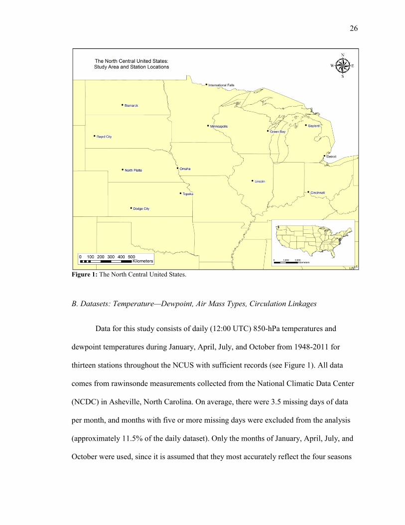
26
Figure 1: The North Central United States.
B. Datasets: Temperature—Dewpoint, Air Mass Types, Circulation Linkages
Data for this study consists of daily (12:00 UTC) 850-hPa temperatures and
dewpoint temperatures during January, April, July, and October from 1948-2011 for
thirteen stations throughout the NCUS with sufficient records (see Figure 1). All data
comes from rawinsonde measurements collected from the National Climatic Data Center
(NCDC) in Asheville, North Carolina. On average, there were 3.5 missing days of data
per month, and months with five or more missing days were excluded from the analysis
(approximately 11.5% of the daily dataset). Only the months of January, April, July, and
October were used, since it is assumed that they most accurately reflect the four seasons

27
of winter, spring, summer, and autumn, respectively, in meteorological terms (Schwartz,
1982).
The use of the 850-hPa level for temperature and dewpoint temperature, rather
than the surface, is preferred in this study because it is close enough to the ground (1200-
1500 meters) to mirror boundary layer conditions, but is fairly conservative and free from
large local-scale variation (Schwartz, 1982; 1995). Thus, geographic disparities in
temperature and dewpoint temperature are consistent at 850-hPa, unlike the irregular
diurnal changes that frequently occur on earth's surface (Schwartz, 1995). Because of this
consistency, the use of 850-hPa data also allows the study area to be properly
characterized with fewer and less dispersed data points than is usually required for
surface measurements (Schwartz, 1991; 1995).
From the daily temperature and dewpoint data, three separate datasets were
derived: 1) average temperatures and dewpoints for each month during the study period,
used to compute baseline trends, 2) air mass types for all non-missing days, assigned via
the numerical temperature and moisture limits from Schwartz (1995), and 3) the average
characteristics for each air mass type – relative frequency, temperature, and dewpoint –
calculated for each month. The resulting seasonal air mass distributions from these air
mass values were then compared with North American 500-hPa pressure patterns from
prior research. Possible changes in general circulation were inferred from the observed
air mass changes taking place (Schwartz, 1995).

28
Chapter V: Methodology
A. Baseline Temperature-Dewpoint Trend Analysis
The first part of the analysis evaluated the changes in station data that were
observed when all days for a given month were grouped together. Monthly averages of
daily 850-hPa temperature and dewpoint temperature were created for each station in the
study area, with each month (January, April, July, and October) representing one of the
four seasons. The resulting monthly time series were then submitted to regression
analysis, in order to detect significant linear trends. The relationship of the simple linear
regression employed is of the form:
y = a + bx + e (Equation 1)
Where y is the dependent (predicted) variable, x is the independent (explanatory)
variable, and e is the error associated with predicting y. In this case, year is the
independent variable, and the temperature or dewpoint value is the dependent variable,
with significance level (p) < .05, and minimum degrees of freedom (df) ≥ 41. IBM SPSS
Statistics (V. 20) was used to conduct these and all subsequent linear trend analyses.
These linear trends function as the ‘baseline’ for detection of air mass modifications,
since sub-group trends hidden within these arbitrary monthly means are exposed by
organizing temperature and dewpoint values into different air mass types (Schwartz,
1995). This process is explained in detail in the subsequent sections of this chapter.
29
B. Application of Integrated Classification Methodology
The next step of the analysis involved assigning each non-missing day during the
four seasons of January, April, July, and October to an air mass category using the
numerical air mass limits identified in Schwartz (1995). These air mass values were
determined using the integrated-method classification, which combines manual trajectory
analysis with automated statistical procedures to produce the final parameters and
transition zones for each seasonal air mass type (see Chapter 2 for a more in-depth
description of this technique).
The integrated-method classification recognizes six air mass types that were used
for this study: Continental (C), originating in central Canada; Pacific (Pa), originating in
the north Pacific Ocean and entering the study area through the Rocky Mountains; Polar
(Po), a combination of Pa and C air occurring only in summer; Dry Tropical (D), derived
from the southwest United States and mostly found in summer; Tropical (T), from the
Gulf of Mexico; and dilute Tropical (dT), a modified form of Tropical occurring in non-
summer months (Schwartz, 1991). The classification also recognizes transitional cases
between two air mass types, designated Unclassed (U). Each air mass in the integrated
classification scheme is defined by a range of temperature and dewpoint values, except
dilute Tropical and Tropical air, which are identified by dewpoint alone (Schwartz, 1991;
1995). Air mass numerical limits for each station vary with season, as well as geographic
location, as a result of modification across the study area (see Figure 2).
In order to assign the air mass categories to the baseline temperature and
dewpoint data, the explicit numerical limits for each station from Schwartz (1995) were

30
coded into a syntax program for IBM SPSS Statistics (V. 20). Daily temperature-
dewpoint data for the individual stations were concatenated, and the program
automatically allocated the corresponding station air mass limits to each of the respective
daily temperature-dewpoint values. Once the air mass parameters were given, monthly
averages of the daily occurrence of each air mass type were created, yielding the relative
frequency of each air mass type. Total and percent frequency for all air mass types were
then calculated for each station during the entire study period (1948-2011). Tabular
outputs of air mass frequency were created for each season (month), as well as isoline
maps; the maps were prepared using ArcGIS ArcMap (V. 10). These outputs served a
twofold purpose: to give a visual interpretation of the spatial disparities present across the
study region for each air mass type, as well as an assessment of the robustness and
accuracy of the classification scheme (Schwartz, 1991).

31
Figure 2: Air mass criteria in January, April, July, and October for the North Central United States (NCUS). Each air
mass is defined by a range of temperature and dewpoint values, except for dilute Tropical (dT) and Tropical (T) air
masses which are identified only by dewpoint. Double-ended arrows show the transition zones, or Unclassed (U) areas.
A range of values indicates that limits vary depending on geographic location within the study area. The air-mass
symbols are: C, Continental; Pa, Pacific; Po, Polar; D, Dry Tropical; dT, dilute Tropical; and T, Tropical. From
Schwartz, 1995.
C. Air Mass Characteristic Trend Analysis
Evaluation of trends involving the derived air mass types was similar to the
procedures outlined in Chapter 4A. First, monthly averages of daily air mass values at
each station during the study period were created. Time series of each air mass type’s
characteristics of relative frequency, 850-hPa temperature, and 850-hPa dewpoint
32
temperature resulted from these monthly averages. Station normals (averages over the
study period for each respective air mass value) were calculated for all variables during
the period of 1981-2010 as well. The next step produced area-wide (mean of all 13
stations) averages of the monthly air mass values of relative frequency, temperature, and
dewpoint (Schwartz, 1995). Area-wide trends served as a diagnostic procedure for
discriminate evaluation of sub-regional air mass characteristic trends, which are
described in Chapter 4D (adapted from Schwartz, 1995). Regression analysis was then
utilized to distinguish linear trends in these monthly air mass values, for both the
individual station and area-wide time series (year = independent variable, air mass value
= dependent variable, p < .05, df ≥ 41).
D. Examination of Sub-Regional Modifications
An evaluation of station air mass characteristic time series showed that if five or
more individual stations showed a significant trend in a given air mass characteristic
(either relative frequency, temperature, or dewpoint), then the corresponding area-wide
(13 station) trend would also be significant. Other statistical diagnostics such as
reasonable goodness of fit (R2 > .01) and sufficient degrees of freedom (df ≥ 41) were
considered in the assessment as well (see Table 1). Subsequent analyses focused on these
larger geographic groupings of air mass features, to more readily identify prominent sub-
regional changes in air masses that might be occurring. For example, an increase in the
frequency of Tropical air at a large number of stations in the eastern part of the NCUS
could point to a significant increase in 500-hPa troughs in the western United States
(Schwartz, 1995). Trends involving four or fewer significant individual stations were
considered ‘minor’ air masses, and were only further inspected to explain modifications

33
in baseline temperature or dewpoint. Trends with five or more significant individual
stations were considered ‘major’ air masses (adapted from Schwartz, 1995). Table 1
below lists the ten air mass values which met this condition, as well as summary statistics
of the criteria used to differentiate the major air masses. Analyses of these major-trend
incidences were performed by first employing the separate station air mass trends created
in chapter 4C. To identify the particular sub-region responsible for the overall air mass
characteristic trend, an aggregate, which only included the individually significant
stations, was created. Each of these time series were converted into departure from 1981-
2010 normals (Schwartz, 1995). Standard errors for each composited air mass time series
were computed using the following formula:
SE = 𝑠
√𝑛 (Equation 2)
Where s is the sample standard deviation, and n is the number of sample observations. In
this case, n ranged from five to eleven possible significant station values. Finally, to
search for possible changes in the observed linear relationships of the air mass time
series, break point estimation was conducted using a piecewise linear regression method.
This procedure, and its validation, is detailed in the next section.

34
Month Air Mass/Characteristic Trend (Sig.) df R2 Stations¹
January Pacific Dewpoint -.041 (.000) 63 0.248 5
April Continental Frequency -.222 (.004) 63 0.128 7
April Dry Tropical Frequency .020 (.001) 63 0.181 5
April Unclassed Frequency .181 (.000) 63 0.328 10
April Pacific Dewpoint -.060 (.000) 63 0.326 6
July Polar Frequency -.298 (.000) 63 0.27 10
July Tropical Frequency .276 (.000) 63 0.306 8
July Unclassed Frequency .094 (.001) 63 0.156 5
July Dry Tropical Temperature .014 (.005) 63 0.122 5
October Pacific Dewpoint -.070 (.000) 63 0.414 11 Table 1: Diagnostics for selection of major air masses. Significant monthly air masses and their
characteristics (relative frequency, temperature, or dewpoint) at the area-wide level are shown,
with corresponding statistics. Linear trends are a composite of all 13 stations for each air mass
value. In order to determine which air masses are considered major, the following criteria were
used: significant area-wide linear trends (p < .05), sufficient degrees of freedom (df ≥ 41),
reasonable model fit (R2 > 0.1), and five or more individual stations with significant linear trends.1
E. Piecewise Linear Regression with Estimated Breakpoints
Piecewise linear regression is a statistical technique used when there are two or
more distinct linear relationships between a response (dependent) variable, y, and an
explanatory (independent) variable, x. In these cases, a single linear model may not
provide an adequate description of the relationship between the variables. Thus,
piecewise linear regression allows multiple linear models to be fit to the data for different
ranges of x. Breakpoints are values of x where the slope of the linear function changes;
typically the value of the breakpoint is unknown and must be estimated (Ryan and Porth,
2007). When there is only one breakpoint, at x=c, the model can be written as:
y = a1 + b1x for x < c (Equation 3)
y = a2 + b2x for x ≥ c

35
Where c is the breakpoint, a1 and a2 are the intercepts before and after the breakpoint,
respectively, while b1 and b2 are the respective slopes before and after the breakpoint. The
terms x < c and x ≥ c are essentially dummy variables, where x < c is 1 if x is less than
the breakpoint value, and 0 if it is above, and x ≥ c is 1 if x is above the breakpoint, and 0
if it is below. In the case of this study, the breakpoint c is the given year from 1948-2011.
The intercept a1 and linear slope b1 for x < c represent the air mass characteristic trend
equation before the given year, and the intercept a2 and linear slope b2 for x ≥ c represent
the trend after the given year. The breakpoints are not constrained to be continuous in this
case (Lemoine, 2012; Schwarz, 2013).
Alternately, the model can be written to test for a change in slope between b1 and
b2. The equation is as follows:
y = b0 + b1(x) + b2(x - c) (Equation 4)
Where b0 is the intercept, b1 is the slope before the break point c, b2 is the difference in
slope after the change point, and (x-c) represents the derived variable from Equation 3.
The null hypothesis is thus H: b2 = 0 which shows no change in slope between x < c and
x ≥ c (Schwarz, 2013).
For the purposes of this study, a simple iterative search method, which estimates
the change points statistically, was used. The method selects from a range of possible
breakpoints and runs a linear regression for each (year = independent variable, air mass
value = dependent variable, p < .05, df ≥ 20). The combined linear model with the
smallest Mean Squared Error (MSE) is then chosen as the final breakpoint value
(Lemoine, 2012; Ryan and Porth, 2007). The combined models are also tested for a

36
change in slope between the two breakpoint values. Any model in which the change is
considered insignificant (H0 accepted) had a single linear trend applied to the entire time
series (1948-2011), and the conclusion was that the series did not have a discernible
breakpoint. IBM SPSS Statistics (V. 20) syntax editor was used to manually input the
potential year ranges for each air mass time series’ breakpoint, and then semi-automated
to compute the statistical model iterations.
Unlike the simple linear regression analyses used by Schwartz (1995), piecewise
linear regression is more applicable in major air mass trend analyses for several reasons.
First, in a recent work by Knight et al. (2008), change points were successfully used to
study changes in air mass frequency in the conterminous United States. Their study used
a similar air mass based classification, the SSC2 (Sheridan, 2002), and was also
conducted on a comparable time series (1948-2005). Second, the time series being used
for this study (1948-2011) is almost twice the length of that used for the Schwartz (1995)
analysis (1958-1992). Though linear regression was appropriate for that work, a number
of climate change studies have pointed out the issues with linear trends if a long time
series is being examined (Menne and Williams, 2005; Tome and Miranda, 2004). Further,
few climate series of even modest chronological length are characterized by only
metrological variation. Even minor changes in a station’s observation practices or
environment, such as site relocation or replacement, can artificially alter the mean level
of measurements (Menne and Williams, 2005).

37
F. General Circulation Linkages
The final part of the analysis assessed the implications of significant air mass
trends on structural climate change in North America. The characteristics and distribution
of significant air mass trends are related to mid latitude general circulation patterns – i.e.
ridge and trough patterns and air flow on the 500-hPa constant pressure surface. Evidence
for this comes from the research of Schwartz and Skeeter (1994), the results of which
concluded that near surface air mass coverage distributions could be related to a small
quantity of meaningful 500-hPa height and surface pressure patterns in all four seasons
(January, April, July, and October). This link found in Schwartz and Skeeter (1994) was
further explored in the results of Schwartz (1995) and related to observed air mass trends.
Air massed based approaches such as Kalkstein et al. (1996), show similar associations
with general circulation patterns, and possible connections were drawn from these works
as well. It should be noted, however, that no new observations concerning the pressure
patterns found in the studies of Schwartz and Skeeter (1994) and Schwartz (1995) have
been made. Possible connections of the air mass patterns found in this study to prior work
must thus be taken with caution, as there is no direct evidence that these patterns have
continued. Following the summaries of seasonal air mass frequency and characteristic
trends (Chapter 5), these conceivable associations are discussed in detail (Chapter 6).
38
Chapter VI: Results
A. Seasonal Air Mass Frequency
This section summarizes the air mass climatology of the NCUS during the four
seasons (January, April, July, and October). The frequency of each air mass type (in
percent) is shown for all stations in the NCUS in Tables 2 through 5. Also included are
isoline maps of the study region, displaying the frequency (in percent) of the air masses
in each season (Figures 3-23). Air masses occurring less than 1% of the time are
considered non-existent, while those with a greater than 50% occurrence are seasonally
dominant (Schwartz, 1991).
i. January
In January, Continental air was the most frequent in the NCUS, with dominant
(greater than 50%) frequency in much of the region, and a strong northeast to southwest
gradient. Areas near Gaylord and International Falls contained C air masses more than
80% of the time; conversely, Continental air was least abundant, but still quite influential,
near North Platte, Topeka, and Dodge City, with coverage about 35-45% of the time
(Table 2; Figure 3). Pacific air had moderate influence in the southwestern part of the
region, but was not dominant anywhere in the NCUS. Pacific air masses had a southwest
to east-northeast gradient, decreasing from greater than 30% near Dodge City in the
southwest, to about 5-10% near Gaylord and International Falls (Table 2; Figure 4).
Unclassed air also had a small to moderate influence in the region (approximately 10-
20%), with an increasing gradient from southwest to northeast (Table 2; Figure 7). Dilute
Tropical and Tropical air masses were the least abundant in winter. Dilute Tropical

39
occurrence was around 9% near Cincinnati, but dropped to less than 1% in the northwest
part of the region, near Rapid City and International Falls (Table 2; Figure 5). Similarly,
Tropical air had its greatest abundance near Cincinnati (about 4%), but quickly decreased
moving northwest, with less than 1% influence in most of the region, above a line from
roughly Gaylord to Dodge City (Table 2; Figure 6). Dry Tropical air masses were not
found in January in the NCUS.
ii. April
In spring, Continental air was dominant in the northern half of the NCUS, and
showed the greatest overall influence, while Pacific air was slightly weaker overall
during this season (Table 3). Continental air had a more latitudinal north-south gradient
than in winter, though more varied and not as greatly widespread in the north; the
percentage of C air masses ranged from roughly 65-70% near Gaylord and International
Falls, to approximately 25% by Dodge City and Topeka (Table 3; Figure 8). Pacific air
ranged from roughly 25% near Dodge City at its greatest, to less than 10% above Green
Bay and Detroit (Table 3; Figure 9). Unclassed air was somewhat stronger than in
January, with moderate (roughly 15-25%) frequency (Table 3; Figure 13). Tropical and
Dilute Tropical air masses were relatively less rarified in April than in January. Tropical
air existed about 15% of the time in the extreme southeast NCUS, but decreased to less
than 5% influence in the north and west (Table 3; Figure 12). Dilute Tropical air occurred
more than 10% of the time near Topeka, Lincoln, and Cincinnati, but dropped to less than
5% in the northwest part of the region, with a loose southeast to northwest pattern (Table
3; Figure 11). Dry Tropical air masses were the least abundant air mass in spring; they
40
occurred around 4% of the time near Dodge City, but rapidly dropped to less than 1%
east and north of Omaha (Table 3; Figure 10).
iii. July
July had four possible air masses: Polar, Tropical, Dry Tropical, and Unclassed.
Continental, Pacific, and Dilute Tropical are all considered non-summer air masses, and
therefore not identified in July (Table 4). Polar air was historically the most abundant,
and showed a strong north-northeast to south-southwest gradient. Polar air was the
dominant air mass in the far north-northeast region of the NCUS, averaging about 55%
near Gaylord and International Falls, but falling to only 5% incidence by Dodge City
(Table 4; Figure 14). Tropical air showed very nearly the opposite gradient, except for the
western portion of the NCUS, which was strongly influenced by Dry Tropical air. The
percentages of T air masses varied considerably from north to south, from about 15-20%
near International Falls and Gaylord, to 45% near Lincoln and Cincinnati, but were not
considered dominant anywhere in the region. Tropical air also varied greatly from east-
southeast to west-northwest, occurring less than 10% near Rapid City, and increasing to
45% near Topeka (Table 4; Figure 16). Conversely, Dry Tropical air had very little
influence in the eastern half of the NCUS, with all stations east of Minneapolis reporting
less than 5% occurrence. The dT gradient increased tightly moving westward, however;
Dry Tropical air was most abundant by Rapid City and North Platte, occurring greater
than 35% of the time (Table 4; Figure 15). Unclassed air had considerable, if not
dominant occurrence in summer (more than all other seasons), varying from about 25%
near International Falls and Detroit, to greater than 40% near Dodge City, and formed a
very ragged west-southwest to east-southeast pattern (Table 4; Figure 17).
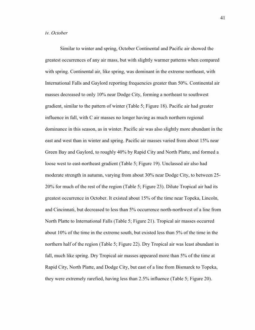
41
iv. October
Similar to winter and spring, October Continental and Pacific air showed the
greatest occurrences of any air mass, but with slightly warmer patterns when compared
with spring. Continental air, like spring, was dominant in the extreme northeast, with
International Falls and Gaylord reporting frequencies greater than 50%. Continental air
masses decreased to only 10% near Dodge City, forming a northeast to southwest
gradient, similar to the pattern of winter (Table 5; Figure 18). Pacific air had greater
influence in fall, with C air masses no longer having as much northern regional
dominance in this season, as in winter. Pacific air was also slightly more abundant in the
east and west than in winter and spring. Pacific air masses varied from about 15% near
Green Bay and Gaylord, to roughly 40% by Rapid City and North Platte, and formed a
loose west to east-northeast gradient (Table 5; Figure 19). Unclassed air also had
moderate strength in autumn, varying from about 30% near Dodge City, to between 25-
20% for much of the rest of the region (Table 5; Figure 23). Dilute Tropical air had its
greatest occurrence in October. It existed about 15% of the time near Topeka, Lincoln,
and Cincinnati, but decreased to less than 5% occurrence north-northwest of a line from
North Platte to International Falls (Table 5; Figure 21). Tropical air masses occurred
about 10% of the time in the extreme south, but existed less than 5% of the time in the
northern half of the region (Table 5; Figure 22). Dry Tropical air was least abundant in
fall, much like spring. Dry Tropical air masses appeared more than 5% of the time at
Rapid City, North Platte, and Dodge City, but east of a line from Bismarck to Topeka,
they were extremely rarefied, having less than 2.5% influence (Table 5; Figure 20).
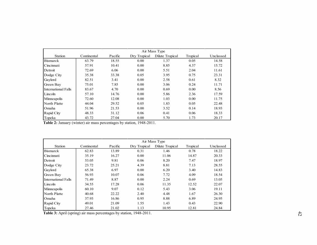
42
Station Continental Pacific Dry Tropical Dilute Tropical Tropical Unclassed
Bismarck 63.79 18.55 0.00 1.37 0.05 14.58
Cincinnati 57.91 10.41 0.00 8.85 4.37 15.72
Detroit 72.69 6.06 0.00 5.51 2.04 11.61
Dodge City 35.38 33.38 0.05 3.95 0.75 23.31
Gaylord 82.51 3.41 0.00 2.58 0.61 8.32
Green Bay 75.01 7.85 0.00 3.06 0.24 11.71
International Falls 83.67 4.70 0.00 0.69 0.00 8.56
Lincoln 57.10 14.76 0.00 5.86 2.36 17.59
Minneapolis 72.60 12.08 0.00 1.03 0.00 11.75
North Platte 44.04 29.52 0.05 1.83 0.05 22.48
Omaha 51.96 21.53 0.00 3.52 0.14 18.93
Rapid City 48.33 31.12 0.06 0.41 0.06 18.33
Topeka 43.72 27.04 0.00 5.70 1.73 20.17
Air Mass Type
Table 2: January (winter) air mass percentages by station, 1948-2011.
Station Continental Pacific Dry Tropical Dilute Tropical Tropical Unclassed
Bismarck 62.83 13.89 0.31 1.46 0.78 18.22
Cincinnati 35.19 16.27 0.00 11.06 14.87 20.33
Detroit 53.05 9.81 0.06 8.20 7.47 18.97
Dodge City 23.72 25.21 4.39 8.81 7.13 28.55
Gaylord 65.38 6.97 0.00 6.20 3.40 14.83
Green Bay 56.93 10.07 0.06 7.72 4.09 18.54
International Falls 71.49 8.87 0.00 2.24 0.69 13.05
Lincoln 34.55 17.28 0.06 11.35 12.52 22.07
Minneapolis 60.10 9.07 0.12 5.43 3.06 19.11
North Platte 40.68 22.22 2.40 4.48 1.67 26.30
Omaha 37.93 16.86 0.95 8.88 6.89 24.95
Rapid City 49.01 21.09 1.55 1.43 0.43 22.90
Topeka 27.46 21.02 1.13 10.95 12.81 24.84
Air Mass Type
Table 3: April (spring) air mass percentages by station, 1948-2011.
43
Station Polar Dry Tropical Tropical Unclassed
Bismarck 35.44 13.08 15.99 34.42
Cincinnati 24.52 2.18 45.81 25.38
Detroit 43.92 2.12 27.74 24.80
Dodge City 5.21 33.09 16.75 43.85
Gaylord 57.62 1.05 18.04 21.73
Green Bay 44.88 1.95 25.62 25.88
International Falls 56.90 2.64 14.43 24.15
Lincoln 21.88 4.02 45.73 27.41
Minneapolis 37.20 4.95 28.70 27.56
North Platte 13.30 36.11 10.48 39.09
Omaha 15.09 12.06 39.50 31.28
Rapid City 23.29 38.13 6.12 31.05
Topeka 11.06 9.94 48.55 29.21
Air Mass Type
Table 4: July (summer) air mass percentages by station, 1948-2011.
Station Continental Pacific Dry Tropical Dilute Tropical Tropical Unclassed
Bismarck 37.68 29.99 1.95 3.70 1.03 23.55
Cincinnati 26.51 25.22 0.00 15.23 9.70 21.98
Detroit 40.17 17.81 0.00 11.64 5.37 22.67
Dodge City 8.38 30.34 6.19 12.94 9.43 30.83
Gaylord 51.24 14.42 0.00 6.86 3.37 20.99
Green Bay 46.10 15.10 0.06 9.25 4.19 22.86
International Falls 53.77 17.77 0.37 4.47 1.39 19.33
Lincoln 25.69 23.62 0.06 14.67 8.75 24.71
Minneapolis 38.32 23.16 0.85 8.43 3.56 22.66
North Platte 18.69 39.78 6.41 3.23 2.54 27.54
Omaha 19.32 30.01 2.00 12.16 7.92 25.55
Rapid City 22.84 40.62 5.44 0.43 2.26 25.99
Topeka 12.58 30.98 1.64 16.05 13.10 23.59
Air Mass Type
Table 5: October (autumn) air mass percentages by station, 1948-2011.

44
Figure 3: Relative frequency (in percent) of Continental air masses, January 1948-2011.
Figure 4: Relative frequency (in percent) of Pacific air masses, January 1948-2011.
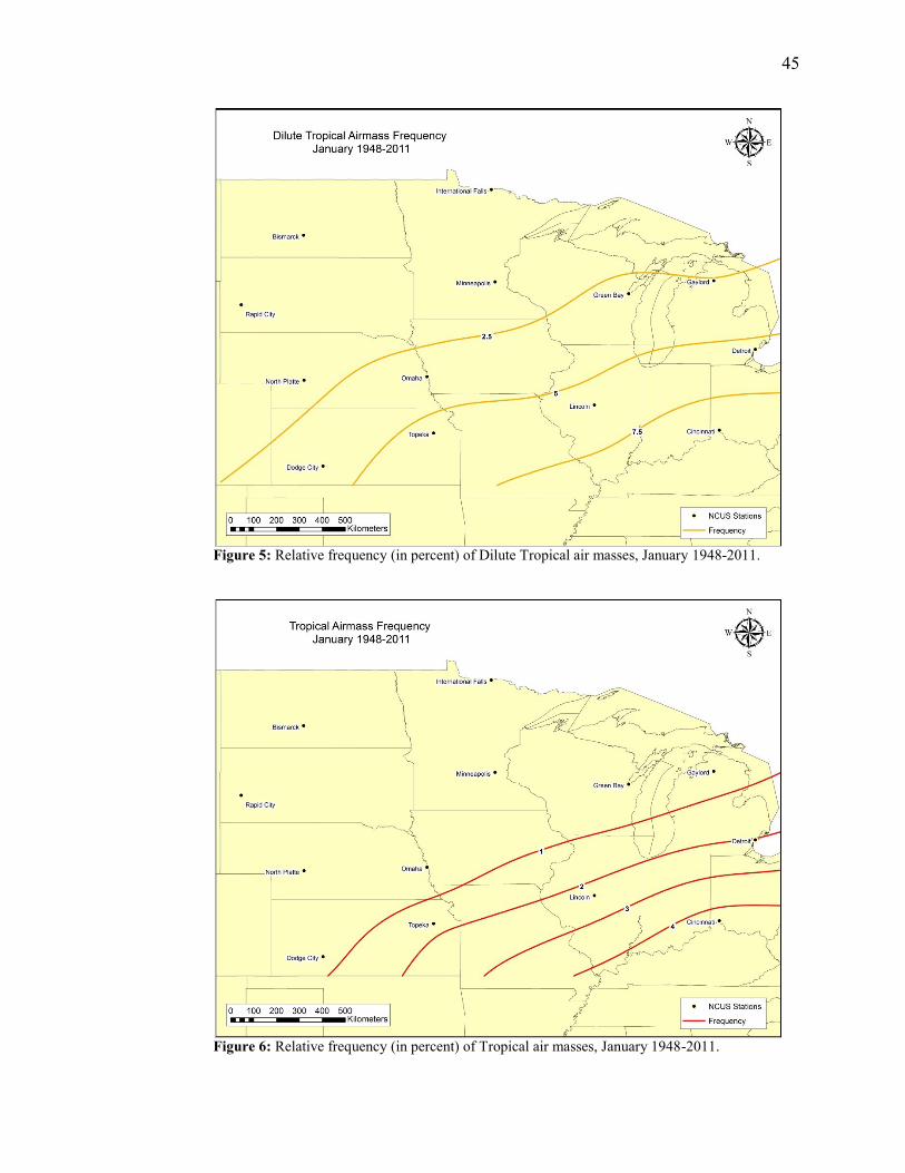
45
Figure 5: Relative frequency (in percent) of Dilute Tropical air masses, January 1948-2011.
Figure 6: Relative frequency (in percent) of Tropical air masses, January 1948-2011.

46
Figure 7: Relative frequency (in percent) of Unclassed air masses, January 1948-2011.
Figure 8: Relative frequency (in percent) of Continental air masses, April 1948-2011.
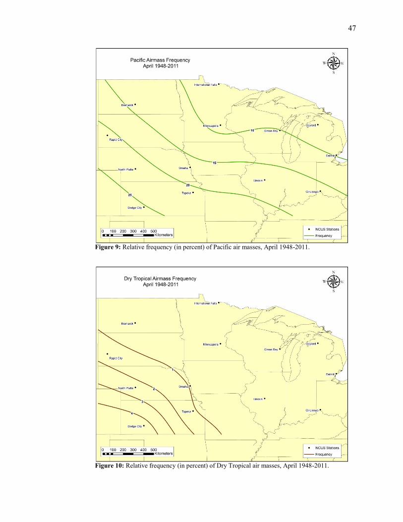
47
Figure 9: Relative frequency (in percent) of Pacific air masses, April 1948-2011.
Figure 10: Relative frequency (in percent) of Dry Tropical air masses, April 1948-2011.

48
Figure 11: Relative frequency (in percent) of Dilute Tropical air masses, April 1948-2011.
Figure 12: Relative frequency (in percent) of Tropical air masses, April 1948-2011.
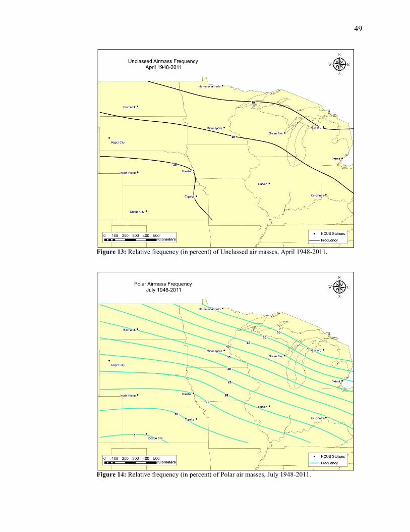
49
Figure 13: Relative frequency (in percent) of Unclassed air masses, April 1948-2011.
Figure 14: Relative frequency (in percent) of Polar air masses, July 1948-2011.
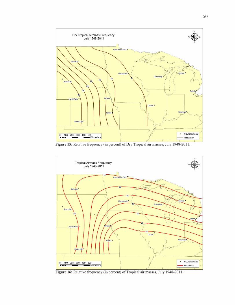
50
Figure 15: Relative frequency (in percent) of Dry Tropical air masses, July 1948-2011.
Figure 16: Relative frequency (in percent) of Tropical air masses, July 1948-2011.

51
Figure 17: Relative frequency (in percent) of Unclassed air masses, July 1948-2011.
Figure 18: Relative frequency (in percent) of Continental air masses, October 1948-2011.

52
Figure 19: Relative frequency (in percent) of Pacific air masses, October 1948-2011.
Figure 20: Relative frequency (in percent) of Dry Tropical air masses, October 1948-2011.

53
Figure 21: Relative frequency (in percent) of Dilute Tropical air masses, October 1948-2011.
Figure 22: Relative frequency (in percent) of Tropical air masses, October 1948-2011.
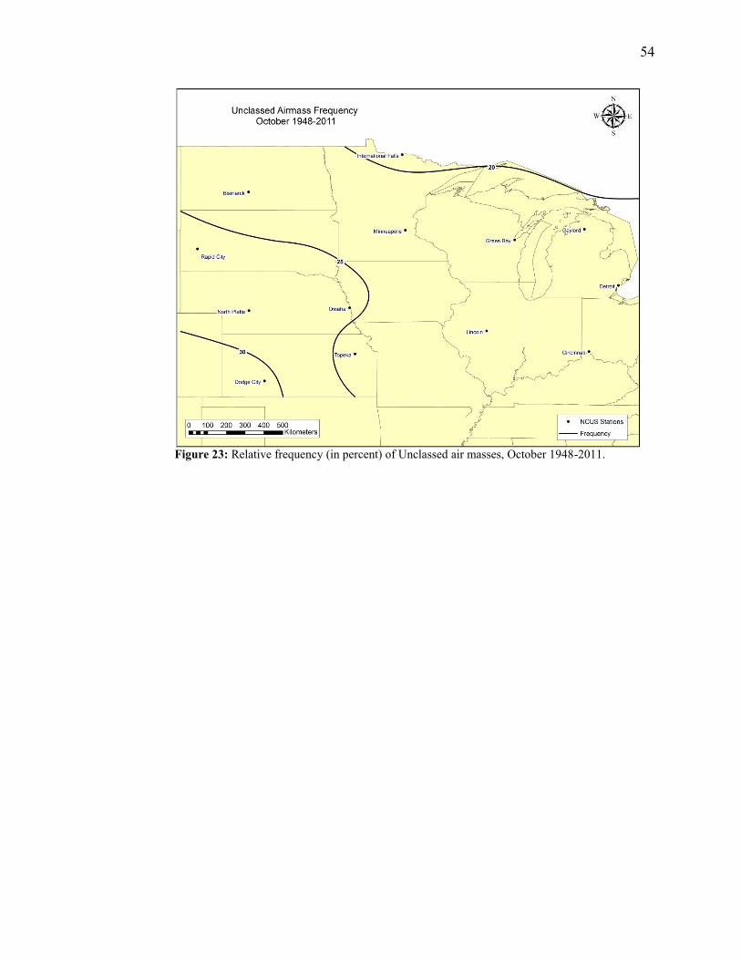
54
Figure 23: Relative frequency (in percent) of Unclassed air masses, October 1948-2011.
55
B. Air Mass Characteristic Trends
In this section, the significant baseline (monthly temperature and dewpoint) and
air mass characteristic trends (relative frequency, air mass temperature, and air mass
dewpoint) are reported. Major air mass linear trends along with their breakpoint values (if
detected) are also described in detail. Trends are either presented in units of degrees
Celsius per year (°C/yr) for temperature and dewpoint, or percent per year (%/yr) for
relative frequency. Data for these results are found in Tables 6-10b, as well as Figures
24-33.
i. January
For January, no significant baseline temperatures or dewpoints were recorded
(Table 6). One air mass was considered major, exhibiting significant trends at five
stations: Pacific air had decreasing dewpoint temperatures which varied from -.022°C/yr
at Dodge City to -.148°C/yr at Cincinnati (Table 8). A similar, though insignificant (p =
.078) trend was reported at Omaha as well. When the five significant stations were
composited, two distinct linear relationships were revealed. From 1948-1979, the trend
appears to be increasing slightly by .026°C/yr, though this trend is not significant (p =
.287, df = 31). From 1980-2011, however, the trend is significant (p = .012, df = 30) and
decreasing by -.083°C/yr (Figure 24).
Significant linear trends in three minor air masses were also observed. Tropical
frequency increased at Cincinnati (.084%/yr) and Gaylord (.032%/yr), but showed an
opposite trend at Dodge City of -.025%/yr (Table 9). Similar upward trends were also
seen at Detroit and Lincoln, but were not significant (p = .055; .052). January Pacific
56
temperature increased significantly at eight stations, though four of these had insufficient
degrees of freedom to be reliable (29 ≤ df ≤ 39), and thus were not considered a major
change (see Chapter 4C and 4D). The four remaining trends varied in size from .027°C/yr
at Rapid City, to .041°C/yr at Bismarck (Table 10a). Finally, Unclassed dewpoint
temperature decreased at Gaylord, by -.07°C/yr (Table 10a).
ii. April
During April, six stations reported significant increases in overall (baseline)
temperature. The increases varied from .033 to .039°C/yr, at Rapid City and Lincoln,
respectively. Similar upward trends were reported at Detroit, Dodge City, and
Minneapolis, though these were not significant (.051 ≤ p ≤ .066). One station,
International Falls, also reported a significant decrease in dewpoint temperature,
-.037°C/yr (Table 6).
Four air masses were considered major in spring. Continental frequency
decreased significantly at six individual stations, varying from -.215%/yr in Topeka, to
-.354%/yr in Lincoln, and mostly occurring in the eastern half of the NCUS (Table 7).
Similar, but insignificant decreases were observed at Dodge City, Gaylord, and Rapid
City (.05 ≤ p ≤ .06) also. When the significant stations were composited, no clear
breakpoint was revealed (H0 accepted), so the simple linear model was used (Figure 25).
The combined decrease in frequency for the six stations was -.323%/yr (p = .00021, df =
63). Dry Tropical frequency significantly increased at five western NCUS stations; the
trends varied from .015 to .114%/yr, at Bismarck and Dodge City, respectively (Table 7).
When composited, the difference in the slopes of the two trends was not considered
57
significant (H0 accepted). Therefore, the single linear model was used (Figure 26), and
found to have a modest increasing trend of .051%/yr (p = .00004, df = 63). Unclassed air
masses also had increasing frequencies at ten significant stations, varying in size from
.14%/yr at Bismarck, to .266%/yr at Green Bay (Table 7). When these stations were
composited, two significant linear fits were produced (Figure 27). From 1948-1988, U air
masses increased at a rate of .158%/yr (p = .011, df = 40). From 1989 onward, however,
the increase was much sharper, at .558%/yr (p = .000042, df = 22). Finally, Pacific
dewpoint temperatures had significantly decreasing trends at six stations in the eastern
NCUS. The temperature trends ranged from -.03°C/yr at Rapid City, to -.154°C/yr at
Detroit (Table 8). When composited, a significant change point was not revealed. The
resulting linear trend for Pa dewpoint (Figure 28) had a -.101°C/yr decrease, though there
was some unusually large variance toward the end of the time series (p = .000, df = 63).
Seven minor air mass values contained stations with significant trends, including
two frequency values (Table 9) and five temperature-dewpoint values (Table 10a). Dilute
Tropical frequency increased at Gaylord (.069%/yr) and Rapid City (.041%/yr). Tropical
frequency also increased in size at Detroit (.106%/yr) and Minneapolis (.068%/yr).
Continental dewpoint decreased at four stations, ranging from -.037 to -.063°C/yr, at
Minneapolis and International Falls, correspondingly. A similar, though insignificant
trend at Detroit (p= .051) was also observed. Dilute Tropical air increased in dewpoint at
Omaha (.013°C/yr), while Tropical air increased in dewpoint at four stations, varying
from .02°C/yr at Cincinnati, to .026°/yr at Detroit. Unclassed air masses increased in
temperature, while at the same time decreasing in dewpoint. One station, Rapid City, had
58
an increase in temperature of .03°C/yr, while dewpoint significantly decreased at
Cincinnati (-.068°C/yr), Detroit (-.064°C/yr), and Gaylord (-.06°C/yr).
iii. July
In summer, ten stations reported upward trends in baseline temperature, and
twelve stations reported upward trends in baseline dewpoint temperature. The trends for
temperature varied in size from .026°C/yr at Cincinnati to .04°C/yr at Detroit, with
Omaha showing a similar, if insignificant trend (p = .064). The trends for dewpoint
temperature ranged from .02°C/yr at North Platte and International Falls, to .048°C/yr at
Cincinnati (Table 6).
Four major air mass changes were observed in July, with three frequency
characteristics (Tables 7), and one temperature characteristic (Table 8). July Polar
frequency decreased significantly at ten stations; the trends ranged in size from -.175%/yr
at Topeka, to -.496%/yr at Gaylord. Similar, though insignificant variations were found at
Omaha (p = .06) and International Falls (p = .056) as well. When the composite time
series was examined for a change point, two distinct relationships were found (Figure
29). From 1948-1972, a very small decreasing trend of -.012%/yr was observed, but was
insignificant (p = .972, df = 24). However, from 1973 onward, the trend was significant
and relatively sharp in decline at -.301%/yr (p = .012, df = 38). Meanwhile, July Tropical
air masses had complementary upward trends in frequency at eight stations in the eastern
and southern NCUS; these ranged from .158%/yr at North Platte, to .409%/yr in
Cincinnati. Similar, though insignificant trends were also observed at Lincoln (p = .063)
and Topeka (p = .087). When the time series were composited, no significant change
59
point was found (H0 accepted). Using a single linear regression model (Figure 30), a
significant increase in Tropical frequency of .282%/yr was shown (p = .000002, df = 63).
Unclassed air increased in frequency at five NCUS stations, ranging from
.126%/yr at Green Bay to .26%/yr at Gaylord. Comparable trends were observed at
International Falls and Rapid City, but these were not significant (p = .068; .077). A
composite trend of the significant stations (Figure 31) revealed two distinct linear
relationships: from 1948-1990, U air was increasing moderately at .106%/yr, but the
trend is just below the significance threshold (p = .056, df = 42). From 1991-2011
however, the trend becomes much steeper (.86%/yr), and significant (p = .000024, df =
20). July Dry Tropical air masses contained warming trends at five western NCUS
stations, varying from .028°C/yr at both Dodge City and Rapid City, to .038°C/yr at
Topeka. A similar, though insignificant trend at Detroit was also reported (p = .053).
When pooled, two disparate linear relationships were revealed (Figure 32). The trend for
D air from 1948-1975 was decreasing, at -.06°C/yr (p = .003, df = 27), while from 1976
onward it increased by .053°C/yr (p = .00001, df = 35).
Six minor air masses also exhibited modifications in this season. Dry Tropical
frequency decreased at Dodge City by -.258%/yr, while simultaneously increasing by
.179%/yr at Rapid City (Table 9). Similar, though insignificant increasing trends at
Lincoln and Topeka were also seen (p = .063; .082). Polar temperature increased at both
Detroit and Gaylord by .023 and .016°C/yr respectively, while Polar dewpoint increased
at Green Bay by .024°C/yr, and Omaha by .035°C/yr (Table 10a). July Tropical
temperature decreased by -.059°C/yr at North Platte and -.103°C/yr at Rapid City, while
increasing by .022°C/yr at Lincoln (Table 10b). Positive trends were observed for July

60
Tropical dewpoint temperature at nine NCUS stations, with one station, Rapid City,
showing a decrease of -.08°C/yr (though increases were observed at five or more stations,
area wide trends were not significant for this air mass value – see Chapter 4D). The size
of the increases ranged from .014 to .033°C/yr at Gaylord and Lincoln, respectively
(Table 10b). July Unclassed temperature increased at four stations, ranging from .02°C/yr
at Bismarck to .04°C/yr at both Dodge City and Omaha (Table 10b). Finally, Unclassed
dewpoints increased at Bismarck (.017°C/yr), Omaha (.023°C/yr), and Rapid City
(.031°C/yr), while concurrently decreasing at Cincinnati (-.035°C/yr), Detroit
(-.031°C/yr), and Gaylord (-.015°C/yr). Similar, but inconsequential changes were seen at
Dodge City (p = .086) and North Platte (p = .061) as well (Table 10b).
iv. October
In October, no significant trends in overall temperature were observed, though
most of the stations had decreases in temperature (Table 6). One station, International
Falls, had a significant decrease in dewpoint of -.031°C/yr, with similar, but insignificant
trends at Green Bay (p =.058) and Rapid City (p = .09).
One major air mass had eleven stations with significant trends: October Pacific air
had decreases in dewpoint ranging from -.028°C/yr at Rapid City, to -.126°C/yr at
Lincoln (Table 8). When the individual stations were pooled, two discrete linear
relationships were exposed (Figure 33). From 1948-1985, a significant, though relatively
modest downward trend of -.076°C/yr was observed for Pa dewpoint (p = .0003, df = 37).
From 1986 to 2011, however, the decrease in dewpoint became much sharper, falling by
-.207°C/yr (p = .002, df = 25).
61
Changes in ten minor air masses were also observed, including five frequency
characteristics (Table 9) and five temperature-dewpoint characteristics (Table 10b).
Continental frequency increased by .21%/yr at International Falls, while Pacific
frequency decreased at Bismarck (-.179%/yr), International Falls (-.142%/yr), and
Minneapolis (-.182%/yr). Dilute Tropical frequency increased in size at one station,
Dodge City, by .125%/yr. October Tropical frequency increased at Cincinnati (.163%/yr),
Detroit (.111%/yr) and Gaylord (.073%/yr), while concurrently reducing in size at North
Platte (-.06%/yr) and Rapid City (-.069%/yr). Unclassed frequency also grew in Rapid
City by .133%/yr, with related, but insignificant trends at Bismarck (p = .077) and North
Platte (p = .063). October Continental temperature, Continental dewpoint, and Pacific
temperature each had one station with a significant trend: a -.025°C/yr decrease at
Topeka, a .072°C/yr increase at Dodge City, and a .019°C/yr increase at Cincinnati,
respectively. Similar trends were observed for Continental temperature at Lincoln and
North Platte, as well as for Continental dewpoint at Bismarck, but none were considered
significant (.056 ≤ p ≤ .083). Dilute Tropical dewpoint had significant upward trends at
four stations, ranging from .011°C/yr at Dodge City and Omaha, to .017°C/yr at Lincoln.
Finally, October Unclassed air masses significantly decreased in dewpoint temperature at
both Detroit (-.084°C/yr) and Green Bay (-.058°C/yr).

62
Station Trend (Sig.) df Trend (Sig.) df Trend (Sig.) df Trend (Sig.) df Trend (Sig.) df Trend (Sig.) df Trend (Sig.) df Trend (Sig.) df
Bismarck .045 (.081) 61 .021 (.287) 61 .034 (.032) 63 .013 (.285) 63 .027 (.038) 62 .034 (.001) 62 -.016 (.322) 62 -.011 (.293) 62
Cincinnati .023 (.279) 53 -.025 (.234) 53 .038 (.004) 53 .000 (.996) 53 .026 (.008) 57 .048 (.000) 57 .011 (.415) 49 -.016 (.398) 49
Detroit .031 (.212) 50 -.022 (.372) 50 .028 (.066) 51 -.018 (.218) 51 .040 (.001) 51 .043 (.000) 51 -.001 (.958) 53 -.022 (.218) 53
Dodge City .013 (.441) 59 -.005 (.698) 59 .028 (.057) 57 -.011 (.522) 57 .027 (.011) 63 .022 (.014) 63 -.014 (.284) 60 .009 (.564) 60
Gaylord .025 (.223) 58 -.009 (.669) 58 .034 (.028) 59 -.022 (.148) 59 .037 (.001) 61 .039 (.000) 61 .005 (.769) 58 -.017 (.246) 58
Green Bay .017 (.459) 52 -.015 (.505) 52 .020 (.211) 57 -.014 (.395) 57 .027 (.025) 57 .047 (.000) 57 -.013 (.433) 56 -.030 (.058) 56
International Falls .024 (.316) 60 -.024 (.257) 60 .017 (.317) 62 -.037 (.009) 62 .011 (.297) 61 .020 (.024) 61 -.026 (.123) 60 -.031 (.031) 60
Lincoln .039 (.077) 53 -.031 (.165) 53 .039 (.012) 53 -.009 (.590) 53 .038 (.003) 53 .036 (.010) 53 .015 (.318) 52 -.027 (.142) 52
Minneapolis .031 (.181) 56 -.023 (.261) 56 .032 (.051) 59 .004 (.799) 59 .018 (.135) 58 .028 (.009) 58 -.018 (.230) 60 -.023 (.147) 60
North Platte .026 (.173) 61 .010 (.502) 61 .020 (.132) 61 .014 (.260) 61 .037 (.001) 62 .020 (.032) 62 -.005 (.750) 60 -.007 (.551) 60
Omaha .005 (.838) 46 -.025 (.192) 46 .027 (.110) 49 .008 (.597) 49 .023 (.064) 52 .042 (.001) 52 -.013 (.388) 49 -.015 (.262) 49
Rapid City .043 (.074) 56 .002 (.915) 56 .033 (.017) 61 .016 (.201) 61 .028 (.020) 63 .004 (.711) 63 -.010 (.519) 59 -.019 (.090) 59
Topeka .036 (.077) 52 -.029 (.116) 52 .035 (.043) 53 -.002 (.897) 53 .033 (.005) 54 .044 (.001) 54 .006 (.656) 54 -.010 (.566) 54
Temperature Dewpoint
January April July October
Temperature Dewpoint Temperature Dewpoint Temperature Dewpoint
Table 6: Baseline temperature-dewpoint trends. Terms included are: Trend, p-value (Sig.) and Degrees of Freedom (df). Highlighted cells are significant at
p < .05, with df ≥ 41.

63
Station Trend (Sig.) df Trend (Sig.) df Trend (Sig.) df Trend (Sig.) df Trend (Sig.) df Trend (Sig.) df
Bismarck -.158 (.092) 63 .015 (.020) 63 .140 (.006) 63 -.295 (.007) 62 .110 (.124) 62 .249 (.000) 62
Cincinnati -.274 (.003) 53 n/a .168 (.011) 53 -.375 (.000) 57 .409 (.000) 57 -.016 (.829) 57
Detroit -.299 (.002) 51 .006 (.104) 51 .253 (.000) 51 -.473 (.000) 51 .336 (.000) 51 .136 (.033) 51
Dodge City -.152 (.052) 57 .114 (.001) 57 .122 (.099) 57 -.056 (.227) 63 .227 (.005) 63 .116 (.215) 63
Gaylord -.214 (.050) 59 n/a .146 (.022) 59 -.496 (.000) 61 .233 (.001) 61 .260 (.000) 61
Green Bay -.225 (.045) 57 .000 (.909) 57 .266 (.000) 57 -.365 (.001) 57 .276 (.004) 57 .126 (.043) 57
International Falls -.087 (.375) 62 n/a .169 (.005) 62 -.196 (.056) 61 .098 (.111) 61 .124 (.068) 61
Lincoln -.354 (.001) 53 .005 (.212) 53 .327 (.000) 53 -.376 (.000) 53 .253 (.063) 53 .059 (.462) 53
Minneapolis -.224 (.044) 59 .008 (.076) 59 .249 (.000) 59 -.325 (.002) 58 .190 (.027) 58 .155 (.014) 58
North Platte -.102 (.254) 61 .057 (.021) 61 .094 (.128) 61 -.257 (.000) 62 .158 (.005) 62 .044 (.599) 62
Omaha -.178 (.096) 49 .024 (.119) 49 .235 (.002) 49 -.135 (.060) 52 .255 (.021) 52 -.020 (.761) 52
Rapid City -.159 (.060) 61 .038 (.022) 61 .180 (.001) 61 -.289 (.002) 63 .037 (.743) 63 .133 (.077) 63
Topeka -.215 (.029) 53 .052 (.005) 53 .091 (.133) 53 -.175 (.009) 54 .241 (.087) 54 .023 (.804) 54
JulyApril April April July July
Frequency
Continental Dry Tropical Unclassed Polar Tropical Unclassed
Frequency Frequency Frequency Frequency Frequency
Table 7: Major air mass frequency trends. Terms included are: Trend, p-value (Sig.) and Degrees of Freedom (df). Highlighted cells are
significant at p < .05, with df ≥ 41.
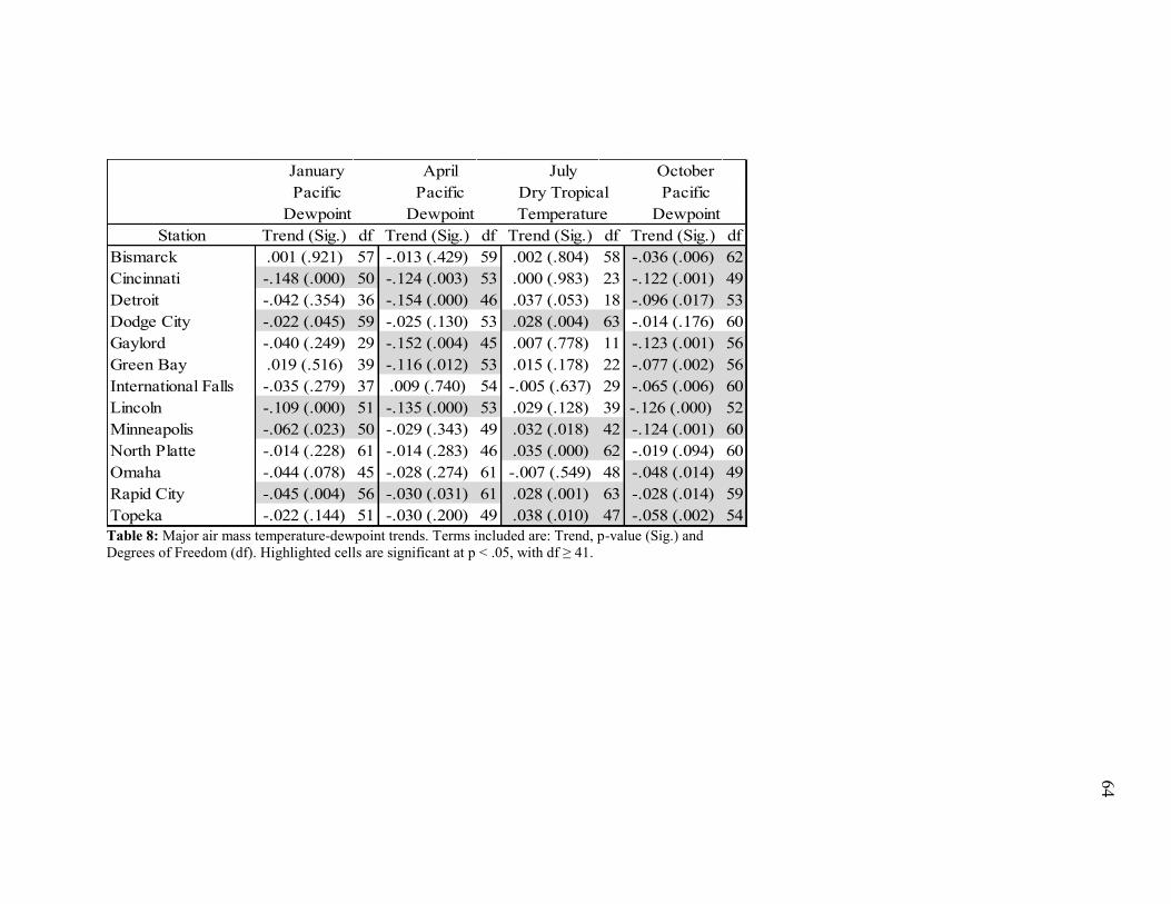
64
Station Trend (Sig.) df Trend (Sig.) df Trend (Sig.) df Trend (Sig.) df
Bismarck .001 (.921) 57 -.013 (.429) 59 .002 (.804) 58 -.036 (.006) 62
Cincinnati -.148 (.000) 50 -.124 (.003) 53 .000 (.983) 23 -.122 (.001) 49
Detroit -.042 (.354) 36 -.154 (.000) 46 .037 (.053) 18 -.096 (.017) 53
Dodge City -.022 (.045) 59 -.025 (.130) 53 .028 (.004) 63 -.014 (.176) 60
Gaylord -.040 (.249) 29 -.152 (.004) 45 .007 (.778) 11 -.123 (.001) 56
Green Bay .019 (.516) 39 -.116 (.012) 53 .015 (.178) 22 -.077 (.002) 56
International Falls -.035 (.279) 37 .009 (.740) 54 -.005 (.637) 29 -.065 (.006) 60
Lincoln -.109 (.000) 51 -.135 (.000) 53 .029 (.128) 39 -.126 (.000) 52
Minneapolis -.062 (.023) 50 -.029 (.343) 49 .032 (.018) 42 -.124 (.001) 60
North Platte -.014 (.228) 61 -.014 (.283) 46 .035 (.000) 62 -.019 (.094) 60
Omaha -.044 (.078) 45 -.028 (.274) 61 -.007 (.549) 48 -.048 (.014) 49
Rapid City -.045 (.004) 56 -.030 (.031) 61 .028 (.001) 63 -.028 (.014) 59
Topeka -.022 (.144) 51 -.030 (.200) 49 .038 (.010) 47 -.058 (.002) 54
Dewpoint Dewpoint Temperature Dewpoint
January April July October
Pacific Pacific Dry Tropical Pacific
Table 8: Major air mass temperature-dewpoint trends. Terms included are: Trend, p-value (Sig.) and Degrees of Freedom (df). Highlighted cells are significant at p < .05, with df ≥ 41.

65
Station Trend (Sig.) df Trend (Sig.) df Trend (Sig.) df Trend (Sig.) df Trend (Sig.) df Trend (Sig.) df Trend (Sig.) df Trend (Sig.) df Trend (Sig.) df
Bismarck -.001 (.643) 61 .005 (.716) 63 -.003 (.801) 63 -.039 (.483) 62 .077 (.417) 62 -.179 (.013) 62 .045 (.267) 62 .000 (.980) 62 .104 (.077) 62
Cincinnati .084 (.043) 53 .018 (.690) 53 .107 (.134) 53 -.003 (.916) 57 -.031 (.750) 49 -.083 (.363) 49 -.074 (.274) 49 .163 (.018) 49 .032 (.693) 49
Detroit .051 (.055) 50 -.045 (.235) 51 .106 (.023) 51 -.002 (.944) 51 -.059 (.642) 53 -.052 (.421) 53 -.093 (.195) 53 .111 (.015) 53 .107 (.157) 53
Dodge City -.025 (.049) 59 -.015 (.760) 57 -.002 (.959) 57 -.258 (.019) 63 .037 (.426) 60 -.091 (.242) 60 .125 (.028) 60 .008 (.894) 60 -.001 (.986) 60
Gaylord .032 (.000) 58 .069 (.046) 59 .026 (.376) 59 .017 (.341) 61 .050 (.610) 58 -.015 (.793) 58 -.012 (.748) 58 .073 (.010) 58 -.012 (.830) 58
Green Bay -.003 (.698) 52 -.018 (.671) 57 .007 (.855) 57 -.005 (.835) 57 .120 (.281) 56 -.080 (.215) 56 -.008 (.862) 56 .018 (.608) 56 .014 (.813) 60
International Falls n/a -.006 (.766) 62 .016 (.142) 62 .026 (.288) 61 .210 (.029) 60 -.142 (.015) 60 .016 (.610) 60 .017 (.353) 60 -.026 (.641) 60
Lincoln .062 (.052) 53 -.027 (.574) 53 .069 (.301) 53 .056 (.063) 53 -.109 (.239) 52 -.034 (.652) 52 -.012 (.866) 52 .077 (.206) 52 .092 (.233) 52
Minneapolis n/a .034 (.312) 59 .068 (.024) 59 .034 (.293) 58 .131 (.170) 60 -.182 (.001) 60 .044 (.320) 60 .036 (.211) 60 .050 (.350) 59
North Platte -.001 (.753) 61 .009 (.773) 61 -.001 (.949) 61 .058 (.543) 62 -.019 (.796) 60 -.091 (.253) 60 .040 (.118) 60 -.060 (.047) 60 .137 (.063) 60
Omaha -.002 (.653) 46 .008 (.865) 49 .033 (.470) 49 -.043 (.515) 52 .109 (.215) 49 .052 (.497) 49 -.002 (.981) 49 .038 (.360) 49 .071 (.250) 49
Rapid City -.001 (.656) 56 .041 (.009) 61 -.007 (.459) 61 .179 (.047) 63 .018 (.840) 59 -.071 (.321) 59 .013 (.092) 59 -.069 (.021) 59 .133 (.032) 59
Topeka .014 (.569) 52 -.004 (.931) 53 .039 (.569) 53 -.126 (.082) 54 .008 (.905) 54 -.076 (.434) 54 .001 (.991) 54 .076 (.247) 54 -.023 (.770) 54
October October October
Tropical Dilute Tropical Tropical Dry Tropical Continental Pacific Dilute Tropical
January April April July October October
Frequency
Tropical Unclassed
Frequency Frequency Frequency Frequency Frequency Frequency Frequency Frequency
Table 9: Minor air mass frequency trends. Terms included are: Trend, p-value (Sig.) and Degrees of Freedom (df). Highlighted cells are significant at
p < .05, with df ≥ 41.

66
Station Trend (Sig.) df Trend (Sig.) df Trend (Sig.) df Trend (Sig.) df Trend (Sig.) df Trend (Sig.) df Trend (Sig.) df Trend (Sig.) df Trend (Sig.) df
Bismarck .041 (.000) 57 -.027 (.213) 59 -.003 (.860) 63 -.012 (.094) 22 -.011 (.902) 12 .015 (.320) 62 .003 (.889) 62 -.002 (.829) 62 .017 (.067) 62
Cincinnati .014 (.293) 50 -.043 (.144) 51 -.007 (.695) 53 .006 (.112) 49 .020 (.006) 52 .000 (.988) 53 -.068 (.023) 53 .014 (.090) 55 -.005 (.751) 55
Detroit .050 (.007) 36 -.071 (.116) 49 -.036 (.051) 51 -.001 (.814) 49 .026 (.011) 44 -.019 (.247) 51 -.064 (.041) 51 .023 (.002) 51 -.012 (.504) 51
Dodge City -.007 (.445) 59 -.033 (.089) 59 .023 (.209) 57 .007 (.086) 51 -.010 (.650) 46 .018 (.261) 57 .004 (.850) 57 -.008 (.542) 34 .000 (.987) 34
Gaylord .064 (.000) 29 -.070 (.028) 50 -.047 (.003) 59 .008 (.084) 46 .004 (.695) 32 -.007 (.540) 57 -.060 (.045) 57 .016 (.023) 61 -.003 (.785) 61
Green Bay .031 (.039) 39 -.009 (.782) 48 -.024 (.137) 57 .003 (.585) 50 .024 (.041) 36 -.012 (.316) 57 -.054 (.054) 57 .007 (.411) 57 .024 (.019) 57
International Falls .043 (.021) 37 -.059 (.097) 48 -.063 (.000) 62 .013 (.082) 31 .010 (.855) 10 .004 (.711) 58 -.043 (.183) 58 .005 (.461) 61 .008 (.245) 61
Lincoln .014 (.234) 51 -.051 (.166) 52 -.053 (.029) 53 .008 (.109) 52 .022 (.014) 49 .022 (.120) 53 -.008 (.701) 53 .012 (.258) 51 -.069 (.188) 51
Minneapolis .034 (.023) 50 -.010 (.733) 52 -.037 (.033) 59 .001 (.785) 41 -.021 (.548) 27 .016 (.175) 56 -.031 (.212) 56 -.001 (.925) 58 .014 (.194) 58
North Platte .031 (.001) 61 -.025 (.152) 61 .015 (.274) 61 .006 (.410) 42 -.050 (.237) 22 .024 (.096) 61 -.002 (.904) 61 -.009 (.305) 57 -.004 (.850) 57
Omaha .013 (.317) 45 -.037 (.151) 44 -.024 (.251) 49 .013 (.009) 45 .007 (.651) 40 .010 (.519) 49 .012 (.450) 49 -.011 (.285) 50 .035 (.021) 50
Rapid City .027 (.029) 56 -.026 (.183) 55 .020 (.157) 61 -.002 (.827) 19 .215 (.487) 5 .030 (.028) 61 .011 (.565) 61 -.005 (.432) 60 .019 (.144) 60
Topeka .020 (.073) 51 -.048 (.140) 52 -.028 (.204) 53 .005 (.231) 50 .012 (.205) 51 .021 (.267) 53 -.023 (.287) 53 -.002 (.865) 47 .035 (.207) 47
January January April April April April April July July
Pacific Unclassed Continental Dilute Tropical Tropical Unclassed Unclassed Polar Polar
Temperature Dewpoint Dewpoint Dewpoint Dewpoint Temperature Dewpoint Temperature Dewpoint
Table 10a: Minor air mass temperature-dewpoint trends. Terms included are: Trend, p-value (Sig.) and Degrees of Freedom (df). Highlighted cells are
significant at p < .05, with df ≥ 41.
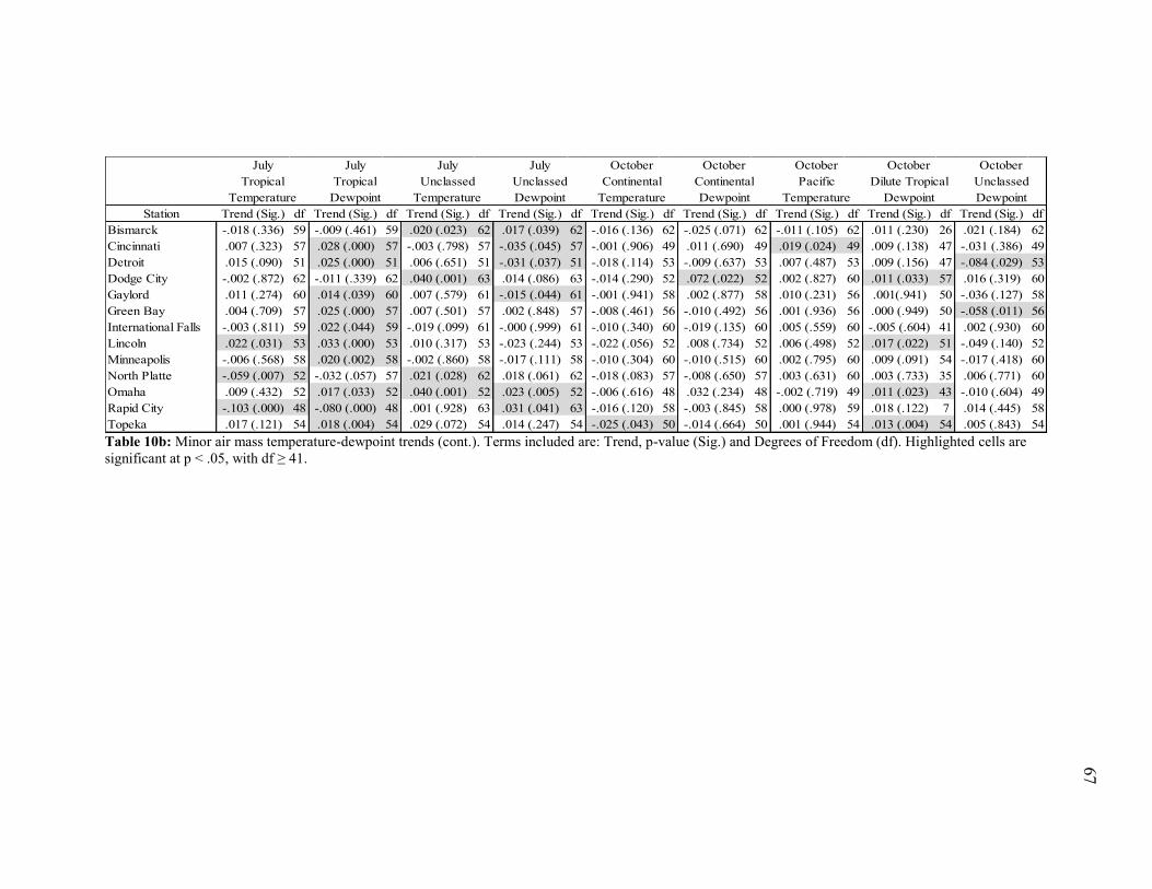
67
Station Trend (Sig.) df Trend (Sig.) df Trend (Sig.) df Trend (Sig.) df Trend (Sig.) df Trend (Sig.) df Trend (Sig.) df Trend (Sig.) df Trend (Sig.) df
Bismarck -.018 (.336) 59 -.009 (.461) 59 .020 (.023) 62 .017 (.039) 62 -.016 (.136) 62 -.025 (.071) 62 -.011 (.105) 62 .011 (.230) 26 .021 (.184) 62
Cincinnati .007 (.323) 57 .028 (.000) 57 -.003 (.798) 57 -.035 (.045) 57 -.001 (.906) 49 .011 (.690) 49 .019 (.024) 49 .009 (.138) 47 -.031 (.386) 49
Detroit .015 (.090) 51 .025 (.000) 51 .006 (.651) 51 -.031 (.037) 51 -.018 (.114) 53 -.009 (.637) 53 .007 (.487) 53 .009 (.156) 47 -.084 (.029) 53
Dodge City -.002 (.872) 62 -.011 (.339) 62 .040 (.001) 63 .014 (.086) 63 -.014 (.290) 52 .072 (.022) 52 .002 (.827) 60 .011 (.033) 57 .016 (.319) 60
Gaylord .011 (.274) 60 .014 (.039) 60 .007 (.579) 61 -.015 (.044) 61 -.001 (.941) 58 .002 (.877) 58 .010 (.231) 56 .001(.941) 50 -.036 (.127) 58
Green Bay .004 (.709) 57 .025 (.000) 57 .007 (.501) 57 .002 (.848) 57 -.008 (.461) 56 -.010 (.492) 56 .001 (.936) 56 .000 (.949) 50 -.058 (.011) 56
International Falls -.003 (.811) 59 .022 (.044) 59 -.019 (.099) 61 -.000 (.999) 61 -.010 (.340) 60 -.019 (.135) 60 .005 (.559) 60 -.005 (.604) 41 .002 (.930) 60
Lincoln .022 (.031) 53 .033 (.000) 53 .010 (.317) 53 -.023 (.244) 53 -.022 (.056) 52 .008 (.734) 52 .006 (.498) 52 .017 (.022) 51 -.049 (.140) 52
Minneapolis -.006 (.568) 58 .020 (.002) 58 -.002 (.860) 58 -.017 (.111) 58 -.010 (.304) 60 -.010 (.515) 60 .002 (.795) 60 .009 (.091) 54 -.017 (.418) 60
North Platte -.059 (.007) 52 -.032 (.057) 57 .021 (.028) 62 .018 (.061) 62 -.018 (.083) 57 -.008 (.650) 57 .003 (.631) 60 .003 (.733) 35 .006 (.771) 60
Omaha .009 (.432) 52 .017 (.033) 52 .040 (.001) 52 .023 (.005) 52 -.006 (.616) 48 .032 (.234) 48 -.002 (.719) 49 .011 (.023) 43 -.010 (.604) 49
Rapid City -.103 (.000) 48 -.080 (.000) 48 .001 (.928) 63 .031 (.041) 63 -.016 (.120) 58 -.003 (.845) 58 .000 (.978) 59 .018 (.122) 7 .014 (.445) 58
Topeka .017 (.121) 54 .018 (.004) 54 .029 (.072) 54 .014 (.247) 54 -.025 (.043) 50 -.014 (.664) 50 .001 (.944) 54 .013 (.004) 54 .005 (.843) 54
Temperature Temperature Dewpoint Temperature DewpointDewpoint
Tropical Unclassed Unclassed Continental ContinentalTropical
July July July October OctoberJuly
Temperature Dewpoint Dewpoint
October October October
Pacific Dilute Tropical Unclassed
Table 10b: Minor air mass temperature-dewpoint trends (cont.). Terms included are: Trend, p-value (Sig.) and Degrees of Freedom (df). Highlighted cells are
significant at p < .05, with df ≥ 41.
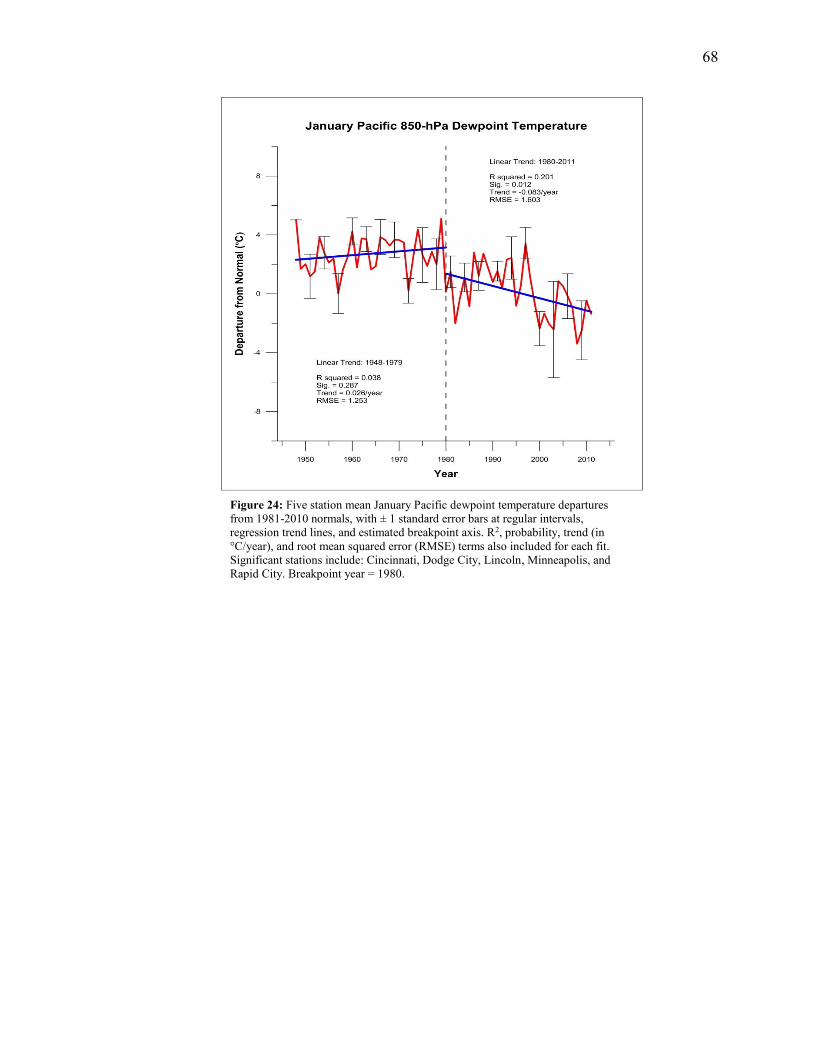
68
Figure 24: Five station mean January Pacific dewpoint temperature departures
from 1981-2010 normals, with ± 1 standard error bars at regular intervals,
regression trend lines, and estimated breakpoint axis. R2, probability, trend (in
°C/year), and root mean squared error (RMSE) terms also included for each fit.
Significant stations include: Cincinnati, Dodge City, Lincoln, Minneapolis, and
Rapid City. Breakpoint year = 1980.
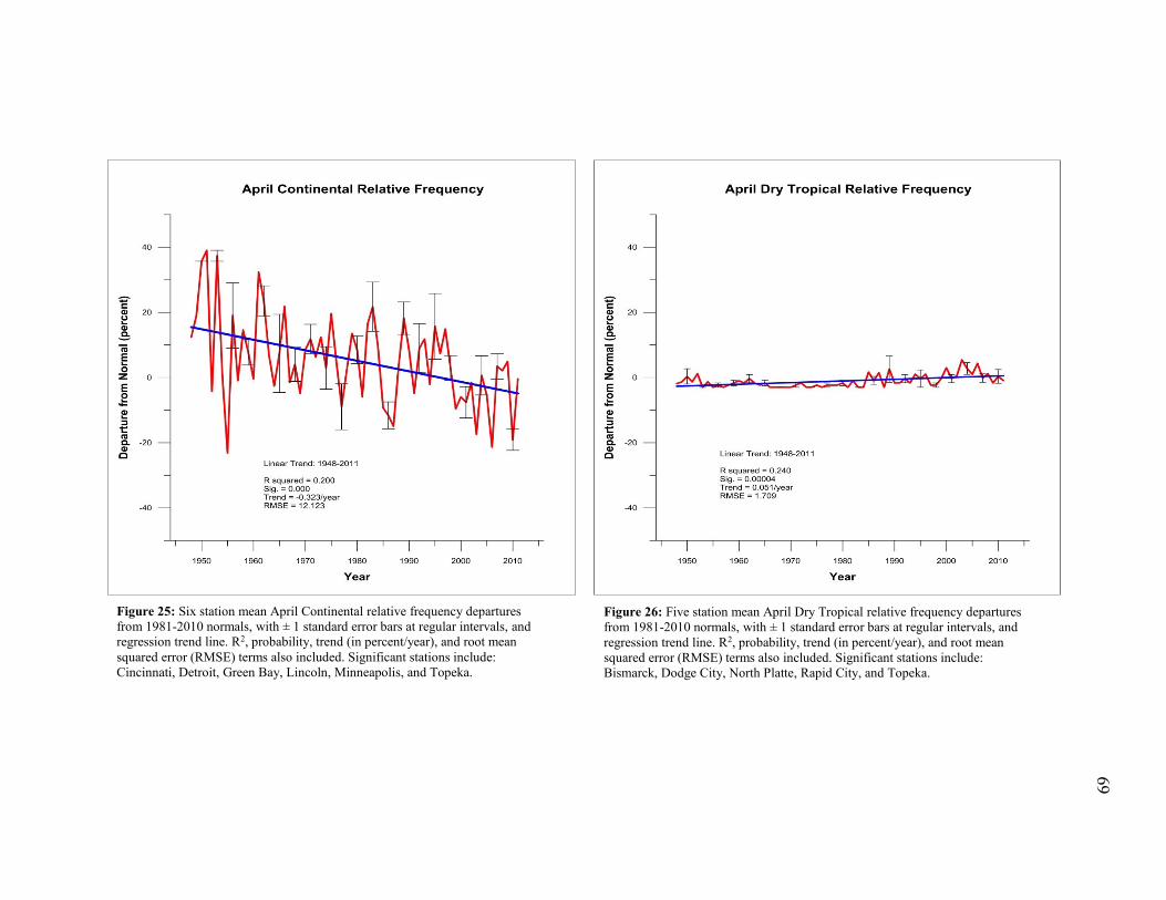
69
Figure 25: Six station mean April Continental relative frequency departures
from 1981-2010 normals, with ± 1 standard error bars at regular intervals, and
regression trend line. R2, probability, trend (in percent/year), and root mean
squared error (RMSE) terms also included. Significant stations include:
Cincinnati, Detroit, Green Bay, Lincoln, Minneapolis, and Topeka.
Figure 26: Five station mean April Dry Tropical relative frequency departures
from 1981-2010 normals, with ± 1 standard error bars at regular intervals, and
regression trend line. R2, probability, trend (in percent/year), and root mean
squared error (RMSE) terms also included. Significant stations include:
Bismarck, Dodge City, North Platte, Rapid City, and Topeka.
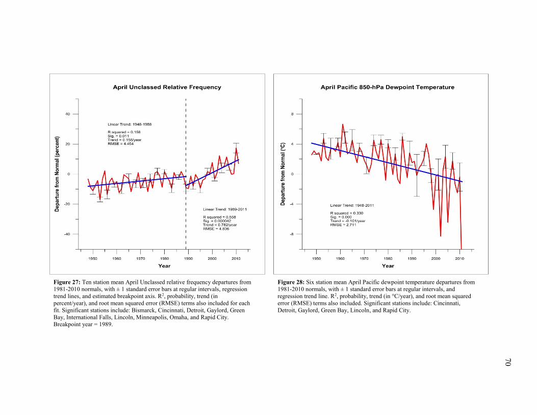
70
Figure 27: Ten station mean April Unclassed relative frequency departures from
1981-2010 normals, with ± 1 standard error bars at regular intervals, regression
trend lines, and estimated breakpoint axis. R2, probability, trend (in
percent/year), and root mean squared error (RMSE) terms also included for each
fit. Significant stations include: Bismarck, Cincinnati, Detroit, Gaylord, Green
Bay, International Falls, Lincoln, Minneapolis, Omaha, and Rapid City.
Breakpoint year = 1989.
Figure 28: Six station mean April Pacific dewpoint temperature departures from
1981-2010 normals, with ± 1 standard error bars at regular intervals, and
regression trend line. R2, probability, trend (in °C/year), and root mean squared
error (RMSE) terms also included. Significant stations include: Cincinnati,
Detroit, Gaylord, Green Bay, Lincoln, and Rapid City.
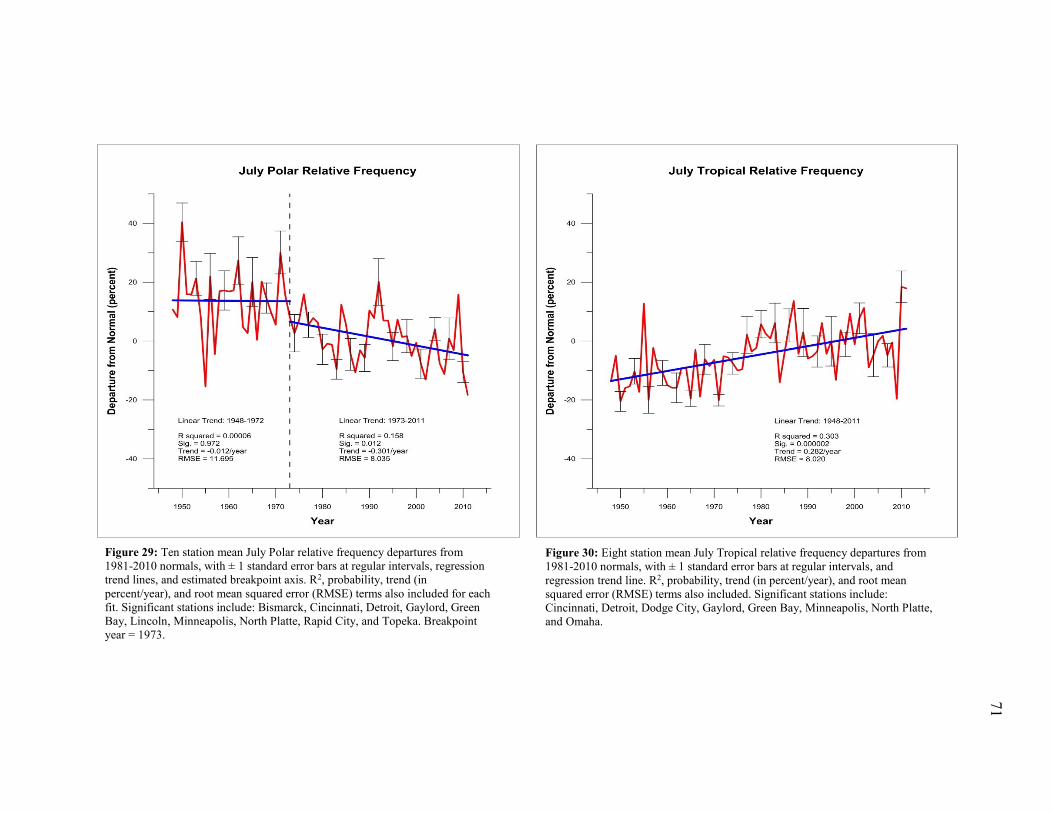
71
Figure 29: Ten station mean July Polar relative frequency departures from
1981-2010 normals, with ± 1 standard error bars at regular intervals, regression
trend lines, and estimated breakpoint axis. R2, probability, trend (in
percent/year), and root mean squared error (RMSE) terms also included for each
fit. Significant stations include: Bismarck, Cincinnati, Detroit, Gaylord, Green
Bay, Lincoln, Minneapolis, North Platte, Rapid City, and Topeka. Breakpoint
year = 1973.
Figure 30: Eight station mean July Tropical relative frequency departures from
1981-2010 normals, with ± 1 standard error bars at regular intervals, and
regression trend line. R2, probability, trend (in percent/year), and root mean
squared error (RMSE) terms also included. Significant stations include:
Cincinnati, Detroit, Dodge City, Gaylord, Green Bay, Minneapolis, North Platte,
and Omaha.
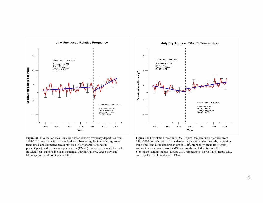
72
Figure 31: Five station mean July Unclassed relative frequency departures from
1981-2010 normals, with ± 1 standard error bars at regular intervals, regression
trend lines, and estimated breakpoint axis. R2, probability, trend (in
percent/year), and root mean squared error (RMSE) terms also included for each
fit. Significant stations include: Bismarck, Detroit, Gaylord, Green Bay, and
Minneapolis. Breakpoint year = 1991.
Figure 32: Five station mean July Dry Tropical temperature departures from
1981-2010 normals, with ± 1 standard error bars at regular intervals, regression
trend lines, and estimated breakpoint axis. R2, probability, trend (in °C/year),
and root mean squared error (RMSE) terms also included for each fit.
Significant stations include: Dodge City, Minneapolis, North Platte, Rapid City,
and Topeka. Breakpoint year = 1976.
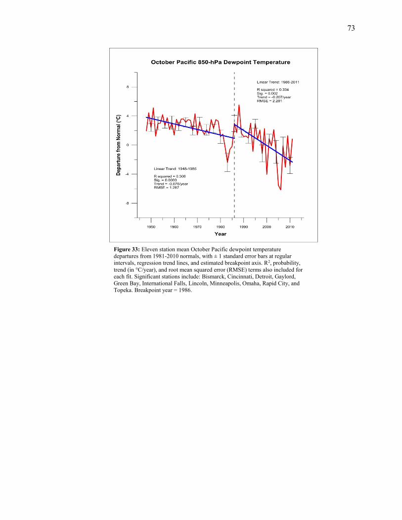
73
Figure 33: Eleven station mean October Pacific dewpoint temperature
departures from 1981-2010 normals, with ± 1 standard error bars at regular
intervals, regression trend lines, and estimated breakpoint axis. R2, probability,
trend (in °C/year), and root mean squared error (RMSE) terms also included for
each fit. Significant stations include: Bismarck, Cincinnati, Detroit, Gaylord,
Green Bay, International Falls, Lincoln, Minneapolis, Omaha, Rapid City, and
Topeka. Breakpoint year = 1986.

74
Chapter VII: Discussion, Conclusions, and Recommendations
A. Discussion
The results of the seasonal air mass climatology confirm that the integrated air
mass limits adopted from Schwartz (1991) are spatially and seasonally consistent. In each
season, air mass distributions across the NCUS follow a logical pattern based on the
varying character of source regions and air mass movement throughout the year.
Continental air masses dominated the region in winter, spring, and autumn, and were
more prominent in the northern portion of the study area. Given the origins of C air in
central Canada, and its southern trajectories, these disparities make sense (Schwartz,
1991). Pacific air had a large number of occurrences in winter and spring, reaching its
greatest influence in autumn, and was more frequent in the western portions of the study
area. Since zonal flow from the northwestern Pacific Ocean marks occurrences of Pacific
air, this sub-regional pattern also seems reasonable (Schwartz, 1982; 1991). Polar air
masses are a modified form of C and Pa air found in summer, and are the dominant air
masses of summer as one moves north. Dilute Tropical and Tropical air masses had their
greatest regional influence in the southeast, with Tropical reaching its peak in summer,
and dilute Tropical peaking in autumn. Warm, moist air from the Gulf of Mexico,
spreading northwest, would cause Tropical air masses to occur most often in summer in
the southeast NCUS, while dilute Tropical air, non-existent in summer, would reach its
peak in the following season. Dry Tropical air masses were a mostly summer
phenomenon, but were found in spring and autumn with greatly reduced strength; their
geographic patterns mainly favored the western NCUS, which is consistent with the
origins of these air masses in the southwest United States, where extremely dry and hot
75
temperatures are common. Finally, patterns of Unclassed air masses were highest in the
southwest part of the NCUS, and most common in summer. This arrangement is likely
due to more air mass mixing in both this area and season. The configurations of these
seasonal air mass distributions are very consistent with those seen in previous research
(Schwartz, 1982; 1991), though there is a slight historical reduction in the total number of
cold air masses at many stations (i.e. C, Po) when compared to the other air masses (i.e.
Pa, dT, T, D, U). This is fairly consistent with the findings of previous studies (Schwartz
and Skeeter, 1994; Schwartz, 1995; Knight et al., 2008; Vanos and Cakmak, 2013). It
should be noted, however, that these data only hint at the changes revealed when the time
series of air mass characteristics are examined. This will subsequently be discussed in
further detail.
In January, no statistically significant changes in baseline temperature and
dewpoint were found, although temperatures were increasing and dewpoints were
decreasing at most NCUS stations. The only major air mass modification, a decrease in
Pacific dewpoint temperature, seems to account for the overall decrease in baseline
dewpoints, and thus was obscured by the baseline trends. This reduction was not
historically consistent however, as until the late 1970’s the trend was essentially flat.
Only from 1980 to present does this trend exhibit a clear negative trend, suggesting this
modification is recent and thus would not have been detected in the results of Schwartz
(1995). A minor increase in Pacific temperature in the northern NCUS, as well as a small
increase in Tropical frequency at three stations was also observed. These warming air
mass patterns appear to reflect the warming of baseline temperature, though their
significance was obscured by the overall trends. The increases in T frequency and Pa
76
temperature should be taken with caution due to their limited geographic scope, but could
suggest a slight increase of warm air masses in winter at the expense of cold air masses at
some stations. Several previous studies have shown patterns of wintertime air mass
warming across the United States and Canada (Kalkstein et al., 1998; Knight et al., 2008;
Vanos and Cakmak, 2013). Knight et al. (2008) notes that a pattern shift of this type is
linked with positive phases of the Arctic Oscillation (AO) for the eastern half of the
United States, specifically the Dry Moderate and Moist Tropical air mass types, which
are comparable to Pa and T air, respectively, in the Schwartz (1991) classification.
Winter warming may also have a connection to contraction of the circumpolar vortex and
decreases in cyclone activity observed at mid-latitudes (Vanos and Cakmak, 2013).
The possible meanings of drying Pacific air, however, are more difficult to pin
down. As this change was not observed in any previous works, interpretations must also
be taken with caution. Because of the major trend decrease in dewpoint temperature
observed, it is possible that this change represents Pa air originating from a different
source, or following a different trajectory. It may also represent an increase in zonal flow
across the Rocky Mountains, which would cause Pa air masses to warm and dry
adiabatically (Schwartz and Skeeter, 1994; Sheridan, 2003). However, because increases
in zonal flow are typically associated with greater frequency of the Pa air mass type
(Schwartz and Skeeter, 1994), and no major warming of Pa air masses has been observed,
the initial conclusion of this work is that this change is most likely related to some sort of
shift in the moisture patterns of the Pa source region in the North Pacific Ocean. It is
unclear what, if any, relation to broader scale circulation patterns this shift in Pa dewpoint
may have.
77
In April, four major air mass modifications occurred, as well as several minor
trends. An increase in the number of Unclassed air masses was seen, with a sharper
upward trend in more recent decades. According to Schwartz and Skeeter (1994),
Unclassed air masses are indicative of a weak trough over the western United States, and
more air mass mixing prior to arrival in the NCUS. Schwartz (1995) also notes that an
increase in U air masses may represent a typological shift in the temperature and moisture
content of another air mass, since it represents the ‘buffer zone’ between two air mass
types. If this is occurring however, it is unclear why it is rapidly increasing. Consistent
with observations in January, a decline in Pacific dewpoint temperature occurred, though
this decrease was much steadier in this season. Again, this may point to source region
changes within the Pa air mass.
A uniform trend towards less Continental air mass days was also seen, while
concurrently, a rise in Dry Tropical days took place. The regression trend line for C air
shows a roughly twenty percent weakening of this air mass over the study period, while
D air masses increased by roughly three percent. Minor air mass characteristic increases
in the frequency of Dilute Tropical and Tropical air also occurred at two stations a piece,
while the dewpoint of C air fell at four eastern NCUS stations. Though Dry Tropical air
is rarified in spring (occurring about two percent of the time in the western part of the
study area), this combination of major and minor effects may be the cause of increased
springtime temperatures observed in the baseline trends. This pattern is similar to the
findings of Schwartz (1995), though the decline of C air is much more prominent here,
and T air masses are not as important. Though not directly comparable, this also
somewhat reflects the findings of Knight et al. (2008), which suggests that cooler spring

78
time air masses are decreasing at the expense of warmer ones. Specifically, they note
decreases in Dry Polar air masses (comparable to C air), and increases in Moist Tropical
air masses.
According to previous work by Schwartz (1982; 1995) and Schwartz and Skeeter
(1994), the decreases in Continental air masses observed in this study could suggest a
weakening in the western U.S. 500-hPa ridge patterns in spring associated with C air.
Though Tropical air is associated with a deepening trough in the western United States,
the strength of T air frequency in this work when compared to that of Schwartz (1995) is
much weaker. Still, it would seem possible that this pattern from the previous study may
have continued. Schwartz (1995) notes that a western 500-hPa trough and concurrent
weakening of the 500-hPa ridge would draw Dry Tropical air into the western part of the
study area, which is seen in this case. This general flow pattern is often related to the
development of severe weather and increases in thunderstorm activity.
The increase in the frequency of Dry Tropical air observed may have a connection
to positive phases of the North Atlantic Oscillation (NAO) as well. Sheridan (2003) notes
that in spring, the source region of Dry Tropical air masses (comparable to Schwartz’s D
air mass type) expands to include much of the northern and central United States. Again,
the observed positive trends in D air masses in the westernmost stations of the NCUS
confirm this. This springtime anomaly further suggests increased westerlies across
Europe during positive phases of the NAO are also observed over North America,
resulting in a greater potential for dry air mass penetration eastward. The increase in D air
in the case of this study is modest, so a link to this teleconnection is somewhat small, but
certainly plausible.

79
In July, almost all NCUS stations reported increases in baseline temperature and
dewpoint. These changes can be explained by four major air mass trends, with two of
them being complementary. Tropical air masses greatly increased in frequency in the
south and east, along with an increase in dewpoint temperature in much of the region
(mainly the east and central areas of the NCUS, but not the far west). The regression line
for T air shows an eighteen percent increase in the frequency of this air mass over the
study period, which is quite considerable. At the same time, Polar air masses decreased in
frequency throughout the NCUS, with a few minor increases in temperature and
dewpoint. The frequency of Polar air did not decline uniformly however. Until the early
1970’s, there was essentially no change in the number of Po air masses, and the true
decline did not begin until after 1972. From 1973 onward, the decline only amounted to
eleven percent, taking place during roughly half the amount of years as T air. This
somewhat differs from the results of Schwartz (1995), which shows (over a smaller time
series) a steadier decline.
In general though, and much like the results in spring, this change further agrees
with previous studies which suggest declines in cooler air masses and increases in
warmer ones (Kalkstein et al., 1998; Knight et al., 2008; Vanos and Cakmak, 2013).
Specifically, these previous works all show increases in Moist Tropical air masses, and
decreases in Dry Polar air masses, while Vanos and Cakmak (2013) show decreases in
Moist Polar air masses (somewhat synonymous with Po air). Knight et al. (2008) also
notes an overall significant negative correlation between the Dry Polar and Moist
Tropical air mass pairs. This pattern shift closely supports the conclusions of Vanos et al.

80
(n.d.) as well, which found similar patterns of warming in the Midwest United States, the
same general region of North America as the NCUS.
In the western NCUS, a change in the temperature of Dry Tropical air was
simultaneously occurring with increases in T air and decreases in Po air, though there are
two distinct relationships involved. Prior to the mid-1970’s, Dry Tropical air was actually
decreasing in temperature, and only from 1976 onward did the temperature increase. This
is markedly different than the results of Schwartz (1995), which notes that the increase
may be a cyclical function; however, with the extra data afforded by the larger time series
in this study, a clearer picture of the relationship can been seen. Interestingly, the increase
in D air temperature fairly closely corresponds with the decline in Po frequency,
suggesting a relationship there as well.
Taking all of these results into account, the relationship between the major air
mass characteristics and circulation patterns in summer still seems to be fairly similar to
the suggestions of Schwartz (1995), even if some of the shifts occurred later than
previously thought. The relationships also point to regional differences as the grounds for
baseline trend increases. Tropical air masses seem to be responsible in the east, while Dry
Tropical air masses are the cause in the west, with Polar air declining throughout the
region. These changes are indicative of amplification of western U.S. 500-hPa trough
patterns, with a coinciding decrease in western U.S. 500-hPa ridge patterns (Schwartz
and Skeeter, 1994). This flow would bring T air into the eastern United States, while
increasing the frequency of D air in the western part of the country. Western troughs also
allow D air to be deposited directly into the western parts of the NCUS, reducing the
potential for air mass cooling from mixing and modification, and thus causing the
81
observed increase in D temperatures (Schwartz, 1982; 1995; Schwartz and Skeeter,
1994). Kalkstein et al. (1998) also notes that an increase in Moist Tropical air masses is
linked with occurrences of semi-permanent ridging in the eastern U.S. and western
Atlantic since the early 1950’s.
Schwartz (1995) points out that Tropical and Dry Tropical air masses are
frequently drawn northeastward by mid-latitude cyclones following their typical
summertime storm track, and an increase in summer T air is associated with more
frequent thunderstorms in the eastern NCUS. Several works, however, show an overall
historical decline in the amount of frontal systems in North America (Harman, 1987;
Ziska and Smith, 1979; Whittaker and Horn, 1981). This decline may be related to a
contraction of the circumpolar vortex noted in some studies, though there is considerable
variability in the contraction and expansion of the vortex over various time series, as well
as in different seasons (Burnett, 1993; Schwartz, 1995; Vanos and Cakmak, 2013).
Finally, Unclassed air masses exhibited a major increase in frequency, with minor
increases in temperature as well. However, this increase in frequency is only significant
starting in the early 1990’s, again, suggesting a very recent effect that would not be seen
in previous studies. Like spring, this trend suggests an increase in air mass mixing en
route, specifically of dT and T air masses (Schwartz, 1982; Schwartz and Skeeter, 1994).
This increase in the frequency of U air may also indicate a recent shift in the character of
one or more air masses (Schwartz, 1995).
In October, a significant decline in baseline dewpoint trends at one station
occurred; the remaining trends for both temperature and dewpoint, though statistically

82
insignificant, were mostly decreasing. One major air mass trend helps to explain the
decrease in baseline dewpoint: Pacific dewpoint temperatures decreased in two distinct
periods. Before the mid-1980’s, the decline was shallow, but after, the decline was much
more rapid. Because of the similarity of this trend’s pattern with those of January and
April, this may represent some kind of recent and rapidly increasing systematic shift in
the dewpoint temperatures of Pacific air masses in all seasons.
There are several minor air mass trends in autumn which appear to have little
relation to broader climate features, so the more prominent ones will be focused on for
possible relations to baseline temperature changes and circulation patterns. First, October
Tropical frequency increased for three stations in the eastern NCUS, while decreasing in
frequency in the west at two stations. Dilute Tropical frequency increased at one station,
and dT dewpoint increased at four stations. These warmer air mass modifications were
masked by the baseline trends, and may help to explain why the decreasing overall
temperature trends were statistically insignificant. In addition, Continental temperature
also decreased throughout the NCUS, though only one station was significant. According
to Schwartz (1995), an amplified 500-hPa trough pattern over the eastern NCUS could
explain many of these patterns. Dilute Tropical air masses, as well as Tropical air in the
east, would be more easily drawn into the study area, while reducing the frequency of T
air masses in the western NCUS. An intensified trough would create more northerly flow,
accounting for cooler and drier C air, and cooler and drier conditions throughout the
NCUS, which are seen in the baseline trends. However, because much of the observed
cooling in baseline trends and C air in autumn is not statistically significant, and those
changes that are significant are relatively minor in scope, these relationships should be
83
interpreted with care. Assuming the patterns of Schwartz’s (1995) study have continued,
this amplification of the 500-hPa ridge-trough pattern would be rather modest compared
to the patterns of spring and summer.
B. Conclusions and Recommendations
This research re-examined the study of Schwartz (1995), using updated and
extended metrological data sets covering the period of 1948-2011. These data formed the
foundation for the classification of air mass types and their characteristics of frequency,
temperature, and dewpoint via the Schwartz (1991) integrated methodology. This study
also improved on the statistical rigor of Schwartz (1995) by incorporating an iterative
change point detection method into the examination of major air mass trends, thus
providing a clearer representation of the changes in their features. The following research
questions were addressed:
1. How are the air mass characteristics of frequency, temperature, and moisture
changing over time?
2. How do these characteristic changes relate to presumed modifications in
atmospheric circulation patterns?
3. How do these results compare to those of previous air mass-based climate
change studies?
Overall, the results showed that the frequency and temperature of warmer air
masses are increasing, while cooler air masses are decreasing in frequency, in spring and
summer seasons. Specifically, the frequency of Continental and Polar air masses declined
84
in spring and summer, respectively. Concurrently, the frequency of Dry Tropical air
increased in spring, while Tropical air mass frequency and Dry Tropical temperature
increased in summer. Additionally, the number of Unclassed air masses increased in
spring and summer, while Pacific air declined in dewpoint temperature. The majority of
these trends in Pacific and Unclassed air, however, are rather recent.
The changes in the character of air masses have been strongly related to several
overlying general circulation patterns, as well as possible associations to teleconnection
features. The decline in spring and summer cold air masses, combined with increases in
warm air, could be indicative of stronger western United States trough patterns, and
weaker ridges. This may also mean increased storm activity in the NCUS (Schwartz,
1995). Other studies point to less cyclonic activity due to a possible contraction of the
circumpolar vortex, which coincides with warming observed in winter and summer
(Burnett, 1993; Vanos and Cakmak, 2013). Possible relationships with the Arctic
Oscillation (AO) and North Atlantic Oscillation (NAO) from modest increases in warm
winter and spring air masses were also observed (Sheridan, 2003; Knight et al., 2008).
Finally, a shift in character of Pacific and Unclassed air masses may be related to source
region changes, increased zonal flow, and air mass mixing (Schwartz and Skeeter, 1994).
The overall decline in cold air masses and increase in warm air masses closely
agree with patterns of surface warming observed (Jones et al., 1999; Hansen et al., 2001;
2010), as well as the results of Schwartz (1995) and other previous air mass based studies
in the Midwest (Vanos et al., n.d.), continental United States (Kalkstein et al., 1998;
Knight et al., 2008), and Canada (Vanos and Cakmak, 2013). The relationships with mid-
tropospheric circulation patterns also follow the results of Schwartz (1995), suggesting

85
those patterns of structural change may be continuing. This study does provide new
insights on some of the major air mass trends, though, that were not observed in Schwartz
(1995). Continental air masses have been shown to be significantly declining in spring,
while Polar and Dry Tropical air masses have patterns that were not previously observed
in summer. Additionally, the decline in Pacific dewpoint temperature in all seasons, and
increases in summer Unclassed air masses are new developments that should be given
further attention to.
Future work should seek greater understanding of the possibility of continued
increases in warm air masses at the expense of cold air masses, their links to increasing
trough and decreasing ridge patterns, and new changes found in Pacific and Unclassed air
masses. A re-examination of the air mass 500-hPa patterns observed in Schwartz and
Skeeter (1994) and Schwartz (1995) is needed to determine if these previous connections
still exist, and if the changes surmised in this study are actually happening. It would be
especially interesting to more readily pinpoint the cause of the systematic modification in
Pacific air masses, and whether this has any connections to large-scale atmospheric
movement. The increases in frequency observed in Unclassed air may be indicative of a
typological shift in other air masses. Future studies may require changes to air mass
temperature and moisture limits if this were to occur. The possible teleconnection
relationships that were implicit in this work, including changes in the AO, NAO, and
circumpolar vortex could be more readily and definitively applied in subsequent studies
of structural climate. These results could have value when applied to resolution of global
climate models at regional scales as well.

86
Literature Cited:
Bejarán, R., & Camilloni, I. (2003). Objective method for classifying air masses: An
application to the analysis of buenos aires’ (argentina) urban heat island intensity.
Theoretical and Applied Climatology, 74(1-2), 93-103. doi: 10.1007/s00704-002-
0714-4
Brunnschweiler, D. H. (1952). The geographic distribution of air masses in north
america. Vierteljahrsschrift Der Naturf., 97, 42-48.
Bryson, R. A. (1966). Air masses, streamlines and the boreal forest. Geographical
Bulletin, 8(3), 228-269.
Burnett, A. W. (1993). Size variations and long-wave circulation within the january
northern hemisphere circumpolar vortex: 1946-89. Journal of Climate, 6(10), 1914-
1920.
Chen, M., Talbot, R., Mao, H., Sive, B., Chen, J., & Griffin, R. J. (2007). Air mass
classification in coastal new england and its relationship to meteorological
conditions. Journal of Geophysical Research: Atmospheres, 112(D10), - D10S05.
doi: 10.1029/2006JD007687
Christensen JR, W. I., & Bryson, R. A. (1966). An investigation of the potential of
component analysis for weather classification. Monthly Weather Review, 94(12),
697-709.

87
Davis, R. E., Dolan, R., & Demme, G. (1993). Synoptic climatology of atlantic coast
north-easters. International Journal of Climatology, 13, 171-189.
doi:10.1002/joc.3370130204
Davis, R. E., & Walker, D. R. (1992). An upper-air synoptic climatology of the western
united states. Journal of Climate, 5(12), 1449-1467.
Davis, R. E., & Kalkstein, L. S. (1990). Development of an automated spatial synoptic
climatological classification. International Journal of Climatology, 10(8), 769-794.
doi:10.1002/joc.3370100802
Dayan, U. (1986). Climatology of back trajectories from israel based on synoptic
analysis. Journal of Climate and Applied Meteorology, 25(5), 591-595.
Frakes, B., & Yarnal, B. (1997). A procedure for blending manual and correlation‐based
synoptic classifications. International Journal of Climatology, 17(13), 1381-1396.
Gaffen, D. J., & Ross, R. J. (1999). Climatology and trends of US surface humidity and
temperature. Journal of Climate, 12(3), 811-828.
Greene, J. S., & Kalkstein, L. S. (1996). Quantitative analysis of summer air masses in
the eastern united states and an application to human mortality. Climate Research,
7(1), 43-53. doi: 10.3354/cr007043
Greene, S., Kalkstein, L. S., Mills, D. M., & Samenow, J. (2011). An examination of
climate change on extreme heat events and climate–mortality relationships in large
U.S. cities. Wea Climate Soc, 3, 281-292.

88
Hansen, J., Ruedy, R., Sato, M., Imhoff, M., Lawrence, W., Easterling, D., Karl, T.
(2001). A closer look at united states and global surface temperature change. Journal
of Geophysical Research: Atmospheres (1984–2012), 106(D20), 23947-23963. doi:
10.1029/2001JD000354
Hansen, J., Ruedy, R., Sato, M., & Lo, K. (2010). Global surface temperature change.
Reviews of Geophysics, 48(4), RG4004. doi: 10.1029/2010RG000345
Harman, J. R. (1987). Mean monthly north american anticyclone frequencies, 1950-79.
Monthly Weather Review, 115(11), 2840-2848.
Jones, G. V., & Davis, R. E. (2000). Using a synoptic climatological approach to
understand climate-viticulture relationships. International Journal of Climatology,
20(8), 813-837.
Jones, P. D., New, M., Parker, D. E., Martin, S., & Rigor, I. G. (1999). Surface air
temperature and its changes over the past 150 years. Reviews of Geophysics, 37(2),
173-199. doi: 10.1029/1999RG900002
Kalkstein, L. S., & Greene, J. S. (1997). An evaluation of climate/mortality relationships
in large U.S. cities and the possible impacts of a climate change. Environ Health
Perspect, 105, 84-93.
Kalkstein, L. S. (1991). A new approach to evaluate the impact of climate on human
mortality. Environmental Health Perspectives, 96, 145.

89
Kalkstein, L. S., Dunne, P. C., & Vose, R. S. (1990). Detection of climatic change in the
western north american arctic using a synoptic climatological approach. Journal of
Climate, 3(10), 1153-1167.
Kalkstein, L. S., Jamason, P. F., Greene, J. S., Libby, J., & Robinson, L. (1996). The
philadelphia hot weather-health watch/warning system: Development and
application, summer 1995. Bulletin of the American Meteorological Society, 77(7),
1519-1528.
Kalkstein, L. S., Nichols, M. C., Barthel, C. D., & Greene, J. S. (1996). A new spatial
synoptic classification: Application to air mass analysis. International Journal of
Climatology, 16(9), 983-1004.
Kalkstein, L. S., Sheridan, S. C., & Graybeal, D. Y. (1998). A determination of character
and frequency changes in air masses using a spatial synoptic classification.
International Journal of Climatology, 18(11), 1223-1236.
Kalkstein, L. S., Tan, G., & Skindlov, J. A. (1987). An evaluation of three clustering
procedures for use in synoptic climatological classification. Journal of Climate and
Applied Meteorology, 26(6), 717-730.
Kalkstein, L. S., & Corrigan, P. (1986). A synoptic climatological approach for
geographical analysis: Assessment of sulfur dioxide concentrations. Annals of the
Association of American Geographers, 76(3), 381-395. doi:10.1111/j.1467-
8306.1986.tb00126.x

90
Knight, D. B., Davis, R. E., Sheridan, S. C., Hondula, D. M., Sitka, L. J., Deaton, M.,
Mazzei, F. (2008). Increasing frequencies of warm and humid air masses over the
conterminous united states from 1948 to 2005. Geophysical Research Letters, 35(10)
doi: 10.1029/2008GL033697
Lamb, H. H. (1972). British isles weather types and a register of the daily sequence of
circulation patterns, 1861-1971. Geophysical Memoirs, 116
Leathers, D. J., Yarnal, B., & Palecki, M. A. (1991). The Pacific/North american
teleconnection pattern and united states climate. part I: Regional temperature and
precipitation associations. Journal of Climate, 4(5), 517-528.
Lemoine, N. (2012). R for ecologists: Putting together a Piecewise Regression. Retrieved
from http://climateecology.wordpress.com/2012/08/19/r-for-ecologists-putting-
together-a-piecewise-regression/
Lund, I. A. (1963). Map-pattern classification by statistical methods. Journal of Applied
Meteorology, 2(1), 56-65.
Makra, L., Mika, J., Bartzokas, A., Béczi, R., Borsos, E., & Sümeghy, Z. (2006). An
objective classification system of air mass types for szeged, hungary, with special
interest in air pollution levels. Meteorology and Atmospheric Physics, 92(1-2), 115-
137. doi: 10.1007/s00703-005-0143-x

91
Marroquin, A., Garcia, J. A., Garrido, J., & Mateos, V. L. (1995). Neyman-scott cluster
model for daily rainfall processes in lower extremadura (spain): Rainfall generating
mechanisms. Theoretical and Applied Climatology, 52, 183-193.
McDonald, N. (1975). Eigenvector analysis as an aid to airmass recognition. Archiv Für
Meteorologie, Geophysik Und Bioklimatologie, Serie A, 24(3), 229-244.
Mearns, L. O., Katz, R. W., & Schneider, S. H. (1984). Extreme high-temperature events:
Changes in their probabilities with changes in mean temperature. Journal of Climate
and Applied Meteorology, 23(12), 1601-1613.
Menne, M. J., & Williams Jr, C. N. (2005). Detection of undocumented changepoints
using multiple test statistics and composite reference series. Journal of Climate,
18(20), 4271-4286.
Merrill, R. M., Shields, E. C., White, G. L. J., & Druce, D. (2005). Climate conditions
and physical activity in the united states. Am J Health Behav, 29, 371-381.
Metzger, K. B., Ito, K., & Matte, T. D. (2010). Summer heat and mortality in new york
city: How hot is too hot? Environmental Health Perspectives, 118(1), 80-86. doi:
10.1289/ehp.0900906; 10.1289/ehp.0900906
Muller, R. A. (1977). A synoptic climatology for environmental baseline analysis: New
orleans. Journal of Applied Meteorology, 16(1), 20-33.
Oort, A. H., & Liu, H. (1993). Upper-air temperature trends over the globe, 1958-1989.
Journal of Climate, 6(2), 292-307.

92
Parker, D., Jones, P., Folland, C., & Bevan, A. (1994). Interdecadal changes of surface
temperature since the late nineteenth century. Journal of Geophysical Research:
Atmospheres (1984–2012), 99(D7), 14373-14399. doi: 10.1029/94JD00548
Pope, C. A. 3rd, & Kalkstein, L. S. (1996). Synoptic weather modeling and estimates of
the exposure-response relationship between daily mortality and particulate air
pollution. Environmental Health Perspectives, 104(4), 414-420.
Ryan, S. E., & Porth, L. S. (2007). A tutorial on the piecewise regression approach
applied to bedload transport data.
Schwartz, M. D. (1982). Air mass climatology of the north central united states. M.S.
Thesis, Department of Geography, Michigan State University.
Schwartz, M. D., Harman, J. R., & Marotz, G. A. (1985). Air mass characteristics over
the north central united states. Geographic Perspectives, 13(56), 13-26.
Schwartz, M. D., & Marotz, G. A. (1986). An approach to examining regional
atmosphere-plant interactions with phenological data. Journal of Biogeography, 13,
551-560.
Schwartz, M. D. (1991). An integrated approach to air mass classification in the north
central united states. The Professional Geographer, 43(1), 77-91.
Schwartz, M. D. (1995). Detecting structural climate change: An air mass-based
approach in the north central united states, 1958–1992. Annals of the Association of
American Geographers, 85(3), 553-568.

93
Schwartz, M. D., & Skeeter, B. R. (1994). Linking air mass analysis to daily and monthly
mid‐tropospheric flow patterns. International Journal of Climatology, 14(4), 439-
464.
Schwarz, C. J. (2013). Regression - hockey sticks, broken sticks, piecewise, change
points. Sampling, regression, experimental design and analysis for environmental
scientists, biologists, and resource managers (pp. 1146-1170)
Sheridan, S. C., & Kalkstein, L. S. (2004). A synoptic climatological approach to
separate weather- and pollution-induced impacts on human mortality. Epidemiology,
15((4), S40.
Sheridan, S. C. (2002). The redevelopment of a weather‐type classification scheme for
north america. International Journal of Climatology, 22(1), 51-68.
Sheridan, S. C. (2003). North american weather‐type frequency and teleconnection
indices. International Journal of Climatology, 23(1), 27-45.
Sheridan, S. C., Allen, M. J., Lee, C. C., & Kalkstein, L. S. (2012). Future heat
vulnerability in california, part II: Projecting future heat-related mortality. Climatic
Change, 115(2), 311-326. doi: 10.1007/s10584-012-0437-1
Solomon, S., D., Qin, M., Manning, Z., Chen, M., Marquis, K. B., Averyt, M.,
(Eds.).IPCC, 2007: Summary for policymakers. in: Climate change 2007: The
physical science basis. contribution of Working Group I to the fourth assessment
94
report of the intergovernmental panel on climate change. Cambridge, United
Kingdom and New York, NY, USA: Cambridge University Press.
Sweeney, J. C., & O’Hare, G. P. (1992). Geographical variations in precipitation yields
and circulation types in britain and ireland. Transactions-Institute of British
Geographers, 17, 448-463.
Tomé, A., & Miranda, P. (2004). Piecewise linear fitting and trend changing points of
climate parameters. Geophysical Research Letters, 31(2) doi:
10.1029/2003GL019100
Vanos, J., & Cakmak, S. (2013). Changing air mass frequencies in canada: Potential links
and implications for human health. International Journal of Biometeorology, 1-15.
Vanos, J., Kalkstein, L., & Sanford, T. Detecting synoptic warming trends across the US
midwest and implications to human health and heat-related mortality.
Whittaker, L. M., & Horn, L. H. (1981). Geographical and seasonal distribution of north
american cyclogenesis, 1958-1977. Monthly Weather Review, 109(11), 2312-2322.
Willett, H. C. (1933). American air mass properties.
Ye, H., Kalkstein, L., & Greene, J. (1995). The detection of climate change in the arctic:
An updated report. Atmospheric Research, 37(1), 163-173.

95
Zishka, K. M., & Smith, P. J. (1980). The climatology of cyclones and anticyclones over
north america and surrounding ocean environs for january and july, 1950-77.
Monthly Weather Review, 108(4), 387-401.


