
1 www.mottcorp.com
Reducing HPLC/UHPLC System Noise and Volume with High Performance Static Mixers
By
James K. Steele, PhD, R&D Scientist,
Christopher J. Martino, Chemical Engineer,
and Kenneth L. Rubow, PhD, VP Filtration/Advanced Media Science
Mott Corporation, 84 Spring Lane, Farmington, CT 06032
www.mottcorp.com
September 8, 2017

2 www.mottcorp.com
Abstract
A revolutionary new inline static mixer has been developed and specifically tailored to meet the exacting
demands of high performance liquid chromatography (HPLC) and ultra‐high performance liquid
chromatography (UHPLC) systems. Poor mixing of two or more mobile phase solvents results in a high
signal to noise ratio and, thus, decreased sensitivity. The homogenous static mixing of two or more
solvents, while utilizing the minimal internal volume and physical size of a static mixer, represents the
ultimate criteria for the ideal static mixer. The new static mixer accomplishes this goal via use of a novel
3D printing technology to create a unique 3D structure that achieves improved hydrodynamic static
mixing with the highest percentage reduction in baseline sine wave per unit of internal mixture volume.
Greater than 95% reduction in baseline ripple was achieved using up to 1/2 the internal volume of some
commonly available mixers. This mixer consists of interconnected 3D flow passageways that have varying
cross‐sectional areas and varying path lengths as the fluid transverses across and through complex 3D
geometric shapes. The mixing in the multitude of tortuous flow paths is coupled with localized turbulent
flow and eddies to create mixing on the micro‐, meso‐, and macro‐scale. Computational fluid dynamic
(CFD) modeling was employed in the design of this unique mixer. The test data presented demonstrates
that superior mixing is achieved while minimizing the internal volume in various gradient test conditions,
such as unparalleled mixing for Trifluoroacetic acid (TFA) and water/acetonitrile gradients.

3 www.mottcorp.com
Introduction
Liquid chromatography has been the work horse analytical methodology for many industries such as
pharmaceuticals, crop protection, environmental, forensics, and chemical analysis for 30+ years. The
ability to measure down to the part per million (ppm) levels and lower is critical to innovative
development processes that lay the groundwork for tomorrow’s drug discovery and the protection of
human and environmental health. Low mixing efficiency, resulting in poor signal to noise ratios, has
plagued the chromatography world when it comes to limits of detection and sensitivity. When combining
two solvents for HPLC testing, it is sometimes necessary to induce mixing by external means to
homogenize the two solvents as some solvents do not mix easily. If poor mixing is present, baseline noise
will appear as a sine wave (rise and fall) of the detector signal versus time. At the same time, poor mixing
will both broaden and create asymmetrical peaks leading to reduced analytical efficiency and peak
resolution. The ideal static mixer will combine the advantages of high mixing efficiency, low dead volume
and low pressure drop, while minimizing the volume and maximizing the throughput of the system.
PerfectPeak® Static Mixers from Mott
Mott recently developed a new line of PerfectPeak® in‐line static mixers with five different internal
volumes: 25 µL, 50 µL, 100 µL, 150 µL, and a prototype 300 µL. These sizes cover the range of volumes
and mixing performance needed for the majority of HPLC testing where enhanced mixing with low
dispersion is required. All five models are 0.5 inches in diameter and have corresponding lengths of 1.4,
1.7, 2.4, 2.7 and 4.5 inches. They are fabricated in 316L stainless steel and passivated for inertness. These
mixers are also available in Titanium and other corrosion resistant and chemically inert alloys. The
maximum operating pressure is 20,000 psig.
Presented in Figure 1a is a photograph of the Mott 100 µL static mixer developed for maximum mixing
efficiency while utilizing a smaller internal volume comparable to standard mixers in this category. This
new static mixer design utilizes a novel additive manufacturing technology to create a unique 3D structure
that achieves high performance mixing. This mixer consists of interconnected three‐dimensional flow
passageways that have varying cross‐sectional areas and varying path lengths as the fluid transverses
through and across internal complex geometric obstacles. Shown in Figure 1b is a schematic
representation of this new mixer utilizing industry standard 10‐32 threaded HPLC compression fittings for
the inlet and outlet, with the boundary of the patent pending internal flow path of the mixer shaded in

4 www.mottcorp.com
blue. The varying cross‐sectional areas of the internal flow path and directional flow changes within the
internal flow volume produce regions of turbulent and laminar flow that create mixing on the micro‐,
meso‐ and macro‐scales. Computational Fluid Dynamic (CFD) modeling was employed in the design of this
unique mixer to analyze flow patterns and to improve designs prior to fabrication of prototypes for
internal analytical testing and customer beta site evaluations.
(a) (b)
Figure 1. Photograph of a Mott 100 µL static mixer (a) and a schematic representation showing a cross‐section view with the mixer fluid flow path shaded in blue (b).
CFD Modeling
Computational Fluid Dynamics (CFD) simulations of the static mixer performance were performed during
the design stage to assist in the development of efficient designs and to reduce trial and error
experimentation, which can be time consuming and expensive. CFD modeling of the Mott static mixer
designs was performed using COMSOL Multiphysics package. Modeling was performed using flowrate‐
driven laminar flow fluid mechanics to understand the fluid velocity, pressure and turbulent nature within
the part. The fluid mechanics interface was coupled with the chemical transport of mobile phase
compounds to help understand the mixing of two different concentrated liquids. The model was studied
under time dependent specifications of 30 seconds for ease of computing while still finding a comparable
solution. Theoretical data was generated in the time dependent study using the point probe projection
tool where a point in the middle of the outlet was selected to gather data. The data was then compared
to the wave function that was specified at the inlet and a relative mixing efficiency was computed.
The CFD model and experimental testing utilized two different solvents through a proportional sampling
valve and pumping system, thereby resulting in alternative plugs of each solvent in the sample line. Prior
to performing simulations through a static mixer, simulations were performed on simple tubing to validate
the model. This initial modeling was performed on a 5 cm long by 0.25 mm ID straight tube to
demonstrate the concept of alternating plugs of water and pure acetonitrile entering the tube with
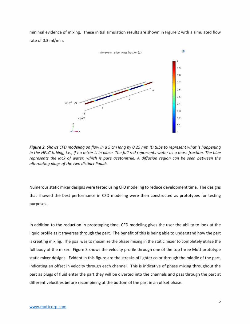
5 www.mottcorp.com
minimal evidence of mixing. These initial simulation results are shown in Figure 2 with a simulated flow
rate of 0.3 ml/min.
Figure 2. Shows CFD modeling on flow in a 5 cm long by 0.25 mm ID tube to represent what is happening in the HPLC tubing, i.e., if no mixer is in place. The full red represents water as a mass fraction. The blue represents the lack of water, which is pure acetonitrile. A diffusion region can be seen between the alternating plugs of the two distinct liquids.
Numerous static mixer designs were tested using CFD modeling to reduce development time. The designs
that showed the best performance in CFD modeling were then constructed as prototypes for testing
purposes.
In addition to the reduction in prototyping time, CFD modeling gives the user the ability to look at the
liquid profile as it traverses through the part. The benefit of this is being able to understand how the part
is creating mixing. The goal was to maximize the phase mixing in the static mixer to completely utilize the
full body of the mixer. Figure 3 shows the velocity profile through one of the top three Mott prototype
static mixer designs. Evident in this figure are the streaks of lighter color through the middle of the part,
indicating an offset in velocity through each channel. This is indicative of phase mixing throughout the
part as plugs of fluid enter the part they will be diverted into the channels and pass through the part at
different velocities before recombining at the bottom of the part in an offset phase.

6 www.mottcorp.com
Figure 3. Velocity profile of liquid in a Mott Static Mixer design. Blue indicates low velocity in the part, red indicates high velocity. It is important to have an offset of velocity throughout the part to induce phase mixing.
The experimental testing utilized two different solvents alternating through a proportional sampling valve
and pumping system, thereby resulting in alternative plugs of each solvent in the sample line. These
solvents were then subsequently mixed in the static mixer. To mimic this in the CFD model, the
assumption was made that the specified inlet function was a representation of no mixing occurring, and
then compared to the wave function from the outlet of the mixer where a mixing efficiency was
calculated. This is best represented in Figure 4 where the green curve is the function specified at the inlet
of the part. The blue curve represents the molar concentration at the outlet of the part, where the peaks
and valleys of the curves are shallower than the specified inlet function. Similar to the experimental data
collection, the amplitudes of the waves are computed, and then the efficiency of the mixer is calculated.

7 www.mottcorp.com
Figure 4. A representation of concentration as a function of time through the Mott static mixer. The green represents the concentration at the inlet of the part while the blue represents the concentration at the outlet of the part.
Experimental Procedure
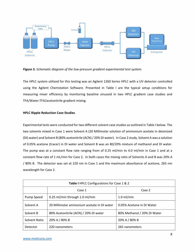
The following HPLC conditions and test setup were used to measure the baseline sine wave to compare
the relative performance of various static mixers. Presented in Figure 5 is a schematic diagram showing
a typical layout of a HPLC/UHPLC system. Testing of static mixers was performed by locating the mixer
immediately downstream of the pump and upstream of the sample injector and HPLC column. Most
background sinusoid measurements (case study 1 & 2) were performed by bypassing the sample injector
and column using a capillary tube between the static mixer and the UV detector. When analysis of signal
to noise ratios and/or peak shape were evaluated, the system was configured as shown in Figure 5.
INLET
OUTLET
8 www.mottcorp.com
Figure 5. Schematic diagram of the low‐pressure gradient experimental test system.
The HPLC system utilized for this testing was an Agilent 1260 Series HPLC with a UV detector controlled
using the Agilent Chemstation Software. Presented in Table I are the typical setup conditions for
measuring mixer efficiency by monitoring baseline sinusoid in two HPLC gradient case studies and
TFA/Water:TFA/acetonitrile gradient mixing.
HPLC Ripple Reduction Case Studies
Experimental tests were conducted for two different solvent case studies as outlined in Table I below. The
two solvents mixed in Case 1 were Solvent A (20 Millimolar solution of ammonium acetate in deionized
(DI) water) and Solvent B (80% acetonitrile (ACN) / 20% DI water). In Case 2 study, Solvent A was a solution
of 0.05% acetone (tracer) in DI water and Solvent B was an 80/20% mixture of methanol and DI water.
The pump was at a constant flow rate ranging from of 0.25 ml/min to 4.0 ml/min in Case 1 and at a
constant flow rate of 1 mL/min for Case 2. In both cases the mixing ratio of Solvents A and B was 20% A
/ 80% B. The detector was set at 220 nm in Case 1 and the maximum absorbance of acetone, 265 nm
wavelength for Case 2.
Table I HPLC Configurations for Case 1 & 2
Case 1 Case 2
Pump Speed 0.25 ml/min through 1.0 ml/min 1.0 ml/min
Solvent A 20 Millimolar ammonium acetate in DI water 0.05% Acetone in DI Water
Solvent B 80% Acetonitrile (ACN) / 20% DI water 80% Methanol / 20% DI Water
Solvent Ratio 20% A / 80% B 20% A / 80% B
Detector 220 nanometers 265 nanometers
9 www.mottcorp.com
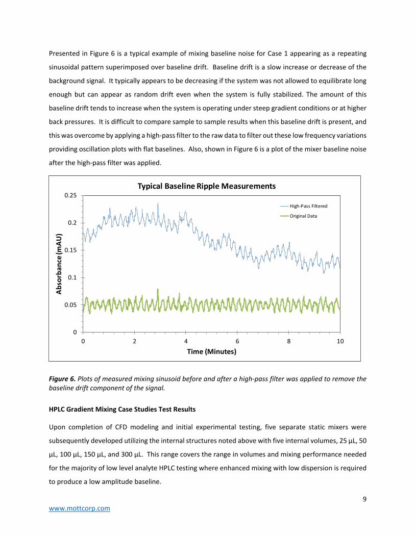
Presented in Figure 6 is a typical example of mixing baseline noise for Case 1 appearing as a repeating
sinusoidal pattern superimposed over baseline drift. Baseline drift is a slow increase or decrease of the
background signal. It typically appears to be decreasing if the system was not allowed to equilibrate long
enough but can appear as random drift even when the system is fully stabilized. The amount of this
baseline drift tends to increase when the system is operating under steep gradient conditions or at higher
back pressures. It is difficult to compare sample to sample results when this baseline drift is present, and
this was overcome by applying a high‐pass filter to the raw data to filter out these low frequency variations
providing oscillation plots with flat baselines. Also, shown in Figure 6 is a plot of the mixer baseline noise
after the high‐pass filter was applied.
Figure 6. Plots of measured mixing sinusoid before and after a high‐pass filter was applied to remove the baseline drift component of the signal.
HPLC Gradient Mixing Case Studies Test Results
Upon completion of CFD modeling and initial experimental testing, five separate static mixers were
subsequently developed utilizing the internal structures noted above with five internal volumes, 25 µL, 50
µL, 100 µL, 150 µL, and 300 µL. This range covers the range in volumes and mixing performance needed
for the majority of low level analyte HPLC testing where enhanced mixing with low dispersion is required
to produce a low amplitude baseline.
0
0.05
0.1
0.15
0.2
0.25
0 2 4 6 8 10
Absorban
ce (m
AU)
Time (Minutes)
Typical Baseline Ripple Measurements
High‐Pass Filtered
Original Data

10 www.mottcorp.com
Water/Acetonitrile Data and Results
Presented in Figure 7 are the results of baseline sine wave measurements taken from the test system for
Case 1 (Acetonitrile with ammonium acetate as a tracer) shown using Mott’s standard volumes of static
mixers along with no mixer installed. The experimental test conditions for the results shown in Figure 7
were held constant for all 4 tests following procedure outlined in Table I with a solvent flow rate of 0.5
ml/min. Offset values were applied to the data set so they could be displayed next to each other without
signal overlap. The offset does not affect the amplitude of the signal which is used to rate the mixer
performance levels. The average amplitude of the sine wave with no mixer installed was 0.18 mAu with
the amplitude dropping to 0.10, 0.06, 0.05, 0.03 and 0.01 mAu for the Mott 25 µL, 50 µL, 100 µL, 150 µL
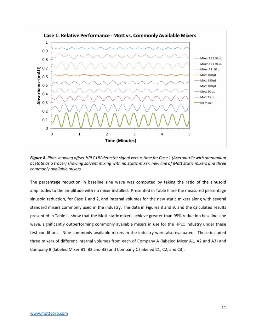
and 300 µL static mixers, respectively. Presented in Figure 8 is the same data as in Figure 7, but with
additional data showing a comparison to commonly available competitive mixers on the market today.
Figure 7. Plots showing offset HPLC UV detector signal versus time for Case 1 (Acetonitrile with ammonium acetate tracer) showing solvent mixing with no mixer, and Mott 25 µL, 50 µL, 100 µL, 150 µL, and 300 µL mixers installed showing improved mixing (smaller signal amplitudes) as the volume of the static mixer is increased.
0
0.1
0.2
0.3
0.4
0.5
0.6
0.7
0.8
0 1 2 3 4 5
Absorban
ce (m
AU)
Time (Minutes)
Relative Performance ‐ Mott 25, 50, 100, 150, & 300 µL
Mott 300 µL
Mott 150 µL
Mott 100 µL
Mott 50 µL
Mott 25 µL
No Mixer
11 www.mottcorp.com
Figure 8. Plots showing offset HPLC UV detector signal versus time for Case 1 (Acetonitrile with ammonium acetate as a tracer) showing solvent mixing with no static mixer, new line of Mott static mixers and three commonly available mixers.
The percentage reduction in baseline sine wave was computed by taking the ratio of the sinusoid
amplitudes to the amplitude with no mixer installed. Presented in Table II are the measured percentage
sinusoid reduction, for Case 1 and 2, and internal volumes for the new static mixers along with several
standard mixers commonly used in the industry. The data in Figures 8 and 9, and the calculated results
presented in Table II, show that the Mott static mixers achieve greater than 95% reduction baseline sine
wave, significantly outperforming commonly available mixers in use for the HPLC industry under these
test conditions. Nine commonly available mixers in the industry were also evaluated. These included
three mixers of different internal volumes from each of Company A (labeled Mixer A1, A2 and A3) and
Company B (labeled Mixer B1, B2 and B3) and Company C (labeled C1, C2, and C3).
0
0.1
0.2
0.3
0.4
0.5
0.6
0.7
0.8
0.9
1
0 1 2 3 4 5
Absorbance (m
AU)
Time (Minutes)
Case 1: Relative Performance ‐Mott vs. Commonly Available Mixers
Mixer A3 250 µL
Mixer A2 150 µL
Mixer A1 50 µl
Mott 300 µL
Mott 150 µL
Mott 100 µL
Mott 50 µL
Mott 25 µL
No Mixer

12 www.mottcorp.com
Figure 9. Plots showing offset HPLC UV detector signal versus time for Case 2 (Methanol with acetone as a tracer) showing solvent mixing with no static mixer (union), new line of Mott static mixers and two commonly available mixers.
Table II Static Mixer Mixing performance and Internal Volumes
Static Mixer Case 1: Sinusoid Reduction: Acetonitrile testing (Efficiency)
Case 2: Sinusoid Reduction: Methanol Water test (Efficiency)
Mott 25 µL 27.3% 21.3% Mott 50 µL 56.0% 47.3% Mott 100 µL 71.3% 70.4% Mott 150 µL 78.4% 79.9% Mott 300 µL 94.5% 95.9%
Mixer A1 (50 µL) 48.0% 49.7% Mixer A2 (150 µL) 68.8% 77.7% Mixer A3 (250 µL) 84.0% 88.7% Mixer B1 (35 µL) 31.4% 27.9% Mixer B2 (100 µL) 57.8% 67.6% Mixer B3 (370 µL) 87.1% 87.4% Mixer C1 (100 µL) 34.0% 25.7% Mixer C2 (250 µL) 83.1% 79.1% Mixer C3 (380 µL) 93.0% 86.5%
0
0.1
0.2
0.3
0.4
0.5
0.6
0.7
0.8
0 1 2 3 4 5
Absorban
ce (m
AU)
Time (Minutes)
Case 2: Relative Performance ‐Mott vs. Commonly Available Mixers
Mott 50 µL
Mixer A1 50µL
Mixer B1 35µL
No Mixer
13 www.mottcorp.com
Examination of the results in Figure 8 and Table II show that the Mott 50 µL static mixer has a similar
mixing efficiency to the Mixer B2 100 µL for the Case 1 study, noting that the Mott 50 µL has ½ the internal
volume while achieving similar performance. When the Mott 50 µL mixer was compared to the Mixer A1
50 µL, a significant improvement in mixing efficiency is observed 56% versus 48%. The performance of
the Mott 100 µL mixer compared to the Mixer A2 150 µL, shows a higher ripple reduction efficiency with
a value of 71.3% versus 68.8% again achieving improved performance at a lower internal volume.
Examination of the Mott 300 µL compared to the A3 250 µL mixer clearly shows significantly greater
mixing efficiency, 94.5% versus 84%, with only a marginal increase in internal volume. Similar results and
comparisons can be observed with Mixers B and C. Thus, the new line of Mott PerfectPeak® static mixers
achieve improved mixing efficiencies over comparable competitors’ mixers, but with smaller internal
volumes, thereby providing improved background noise, better signal to noise ratios, better analyte
sensitivity, peak shapes, and peak resolution. Similar trends in the mixing efficiency were observed in
both Case 1 and Case 2 studies.
For the Case 2 study (Figure 9) using (Methanol with acetone as a tracer) testing was performed to
compare the mixing efficiencies of the Mott 50 L, the comparable Mixer A1 (also with a 50 µL internal
volume) and comparable Mixer B1 (with a lower 35 µL internal volume). As expected the performance
when no mixer installed was poor but is used for a baseline of analysis. The Mott 50 L showed
comparable mixer performance to the A1 mixer with significant improvement over the smaller volume B1
mixers. The ripple reduction efficiency for the Mott 50 µL mixer was 47.3%, for the A1 50 µL mixer, the
efficiency was 49.7% and for the B1 35 µL mixer, the mixing efficiency was lower being 27.9%.
Mixer Back Pressure versus Flow Rate
To investigate the differences in back pressure created by the new line of Mott mixers versus the
competitor mixers previously studied, an experiment was performed by installing an external pressure
sensor immediately upstream of the mixer with no fluid lines connected to the mixer outlet and the
pressure was recorded versus flow rate. The solution used for this test was an isocratic mix of 50%
isopropyl alcohol in DI water. Presented in Table III are the results of this study. Here, it is observed in all
cases, the back pressure increases with flow rate as expected. The Mott line of mixers in nearly all cases
create the lowest back pressures of all mixers tested. The one exception is Mixer A3 250 µL mixer which
measured nearly the same back pressures as Mott’s 300 µL mixer for all flow rates tested. A big advantage
of the Mott design having significantly lower back pressures is being able to run higher viscosity mobile
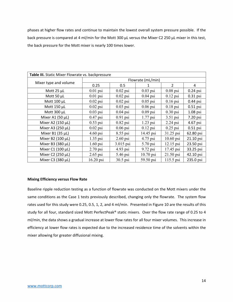
14 www.mottcorp.com
phases at higher flow rates and continue to maintain the lowest overall system pressure possible. If the
back pressure is compared at 4 ml/min for the Mott 300 µL versus the Mixer C2 250 µL mixer in this test,
the back pressure for the Mott mixer is nearly 100 times lower.
Table III. Static Mixer Flowrate vs. backpressure
Mixer type and volume Flowrate (mL/min)
0.25 0.5 1 2 4 Mott 25 µL 0.01 psi 0.02 psi 0.03 psi 0.08 psi 0.24 psi Mott 50 µL 0.01 psi 0.02 psi 0.04 psi 0.12 psi 0.31 psi Mott 100 µL 0.02 psi 0.02 psi 0.05 psi 0.16 psi 0.44 psi Mott 150 µL 0.02 psi 0.03 psi 0.06 psi 0.18 psi 0.51 psi Mott 300 µL 0.03 psi 0.04 psi 0.09 psi 0.30 psi 1.08 psi
Mixer A1 (50 µL) 0.47 psi 0.91 psi 1.77 psi 3.51 psi 7.20 psi Mixer A2 (150 µL) 0.53 psi 0.82 psi 1.23 psi 2.24 psi 4.67 psi Mixer A3 (250 µL) 0.02 psi 0.06 psi 0.12 psi 0.25 psi 0.51 psi Mixer B1 (35 µL) 4.60 psi 8.55 psi 14.45 psi 31.25 psi 62.80 psi Mixer B2 (100 µL) 1.35 psi 2.60 psi 4.75 psi 10.60 psi 21.10 psi Mixer B3 (380 µL) 1.60 psi 3.015 psi 5.70 psi 12.15 psi 23.50 psi Mixer C1 (100 µL) 2.70 psi 4.93 psi 9.72 psi 17.45 psi 33.25 psi Mixer C2 (250 µL) 2.65 psi 5.46 psi 10.70 psi 21.50 psi 42.10 psi Mixer C3 (380 µL) 16.20 psi 30.5 psi 59.50 psi 115.5 psi 235.0 psi
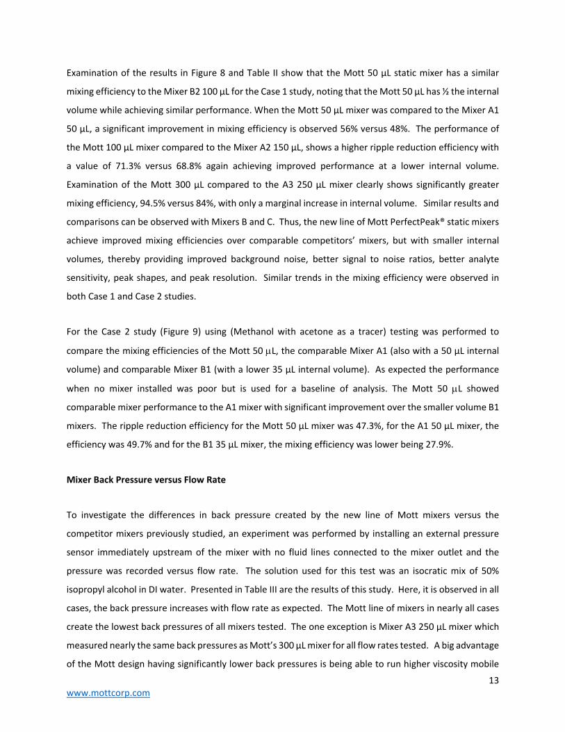
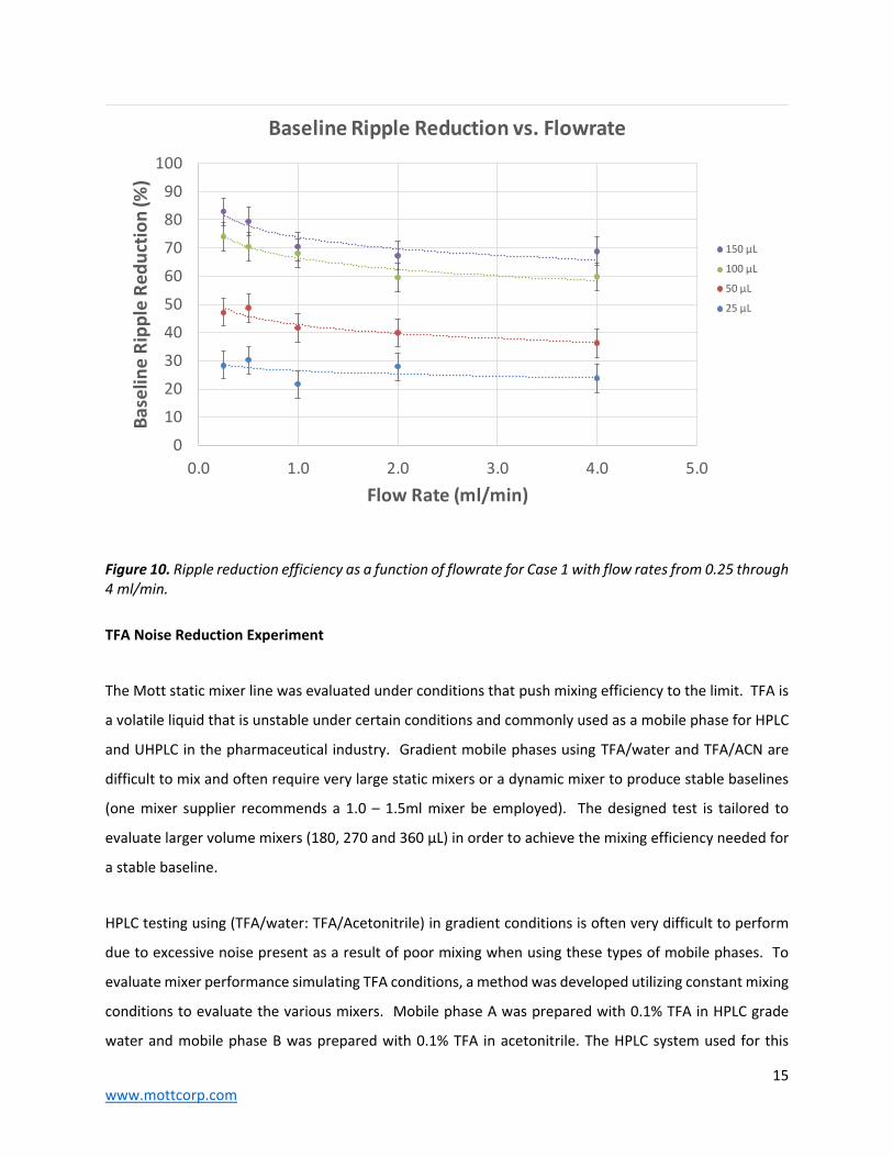
Mixing Efficiency versus Flow Rate
Baseline ripple reduction testing as a function of flowrate was conducted on the Mott mixers under the
same conditions as the Case 1 tests previously described, changing only the flowrate. The system flow
rates used for this study were 0.25, 0.5, 1, 2, and 4 ml/min. Presented in Figure 10 are the results of this
study for all four, standard sized Mott PerfectPeak® static mixers. Over the flow rate range of 0.25 to 4
ml/min, the data shows a gradual increase at lower flow rates for all four mixer volumes. This increase in
efficiency at lower flow rates is expected due to the increased residence time of the solvents within the
mixer allowing for greater diffusional mixing.
15 www.mottcorp.com
Figure 10. Ripple reduction efficiency as a function of flowrate for Case 1 with flow rates from 0.25 through 4 ml/min.
TFA Noise Reduction Experiment
The Mott static mixer line was evaluated under conditions that push mixing efficiency to the limit. TFA is
a volatile liquid that is unstable under certain conditions and commonly used as a mobile phase for HPLC
and UHPLC in the pharmaceutical industry. Gradient mobile phases using TFA/water and TFA/ACN are
difficult to mix and often require very large static mixers or a dynamic mixer to produce stable baselines
(one mixer supplier recommends a 1.0 – 1.5ml mixer be employed). The designed test is tailored to
evaluate larger volume mixers (180, 270 and 360 µL) in order to achieve the mixing efficiency needed for
a stable baseline.
HPLC testing using (TFA/water: TFA/Acetonitrile) in gradient conditions is often very difficult to perform
due to excessive noise present as a result of poor mixing when using these types of mobile phases. To
evaluate mixer performance simulating TFA conditions, a method was developed utilizing constant mixing
conditions to evaluate the various mixers. Mobile phase A was prepared with 0.1% TFA in HPLC grade
water and mobile phase B was prepared with 0.1% TFA in acetonitrile. The HPLC system used for this
0
10
20
30
40
50
60
70
80
90
100
0.0 1.0 2.0 3.0 4.0 5.0
Baseline Ripple Reduction (%
)
Flow Rate (ml/min)
Baseline Ripple Reduction vs. Flowrate
150 µL
100 µL
50 µL
25 µL

16 www.mottcorp.com
analysis was an Agilent 1260 with a binary pump module. The pumps were set to flow at 1 mL/min with
a 95% mobile phase A and 5% mobile phase B mixing ratio. Once the static mixer to be tested was installed
and stabilized, the signal was recorded for 10 minutes. Pump conditions and solution compressibility
factors were set to automatic for this testing. The column was a Waters Symmetry® C18, 5 µm, 3.9 x 150
mm, heated to 30°C. The detector, an Agilent 1100 WVD G1314A, was set at 210 nm wavelength for
analysis.
TFA Data and Results
Figure 11. TFA Stability test data. The given test conditions are as follows: Mobile phase A: 0.1% TFA in DI water, Mobile phase B: 0.1% TFA in acetonitrile, A:B ratio of 95%:5% Flowrate: 1 mL/min, Column: Symmetry® C18, 5 µm, 3.9 x 155 mm at 30°C, Detector: 210 nm.
Presented in Figure 11 are the results comparing Mott’s 150 µL and 300 µL prototype volume mixers to
industry standard Mixer A3 250 µL and Mixer C1 100 µL mixers along with no mixer installed. It is visually
evident that the Mixer B1 100 µL mixer did not perform as well as the other mixers showing little to no
improvement to when no mixer was installed. Mott 150 µL mixer performs very similarly to the Mixer A3
250 µL mixer doing so with about 100 µL less internal volume. The Mott 300 µL mixer provided the lowest
0
2
4
6
8
10
12
14
16
0 2 4 6 8 10
Absorban
ce (m
AU)
Time (Minutes)
TFA Stability Test ‐ Mott vs. Commonly Available Mixers
Mott 300 µL
Mott 150 µL
Mixer A3 250µL
Mixer C1 100µL
No Mixer

17 www.mottcorp.com
and smoothest noise amplitude outperforming the Mixer A3 250 µL mixer with only a minimal increase in
internal volume.
One of the benefits of the Mott PerfectPeak® line of static mixers is their modularity giving you the ability
to achieve different volume combinations. The stackability of the mixers allows for further noise
reduction. Figure 12 shows the baseline stability when stacking our 100 µL and 150 µL mixers in series to
larger internal mixing volumes of 300 µL, 400 µL, and 500 µL. The data in Figure 12 clearly shows a
progression of improved performance as the internal volume increases. The 150 µL Mott mixer shows an
average reduction in amplitude of about 30% and the Mott 300 µL mixer shows a reduction in amplitude
of about 50%. Examination of the larger volume mixers (400 µL and 500 µL) shows further reductions in
noise amplitude with smoother sinusoid waves along with a lower frequency (number of background
ripple humps).
Figure 12. TFA gradient test data. Same test method as stated in Figure 11. Mott 100 µL and 150 µL mixers tested in series to achieve higher internal volume mixing.
0
2
4
6
8
10
12
14
16
0 2 4 6 8 10
Absorban
ce (m
AU)
Time (Minutes)
TFA Stability Test ‐ Large Volume Mixers
Mott 500 µL
Mott 400 µL
Mott 300 µL
Mott 150 µL
No Mixer
18 www.mottcorp.com
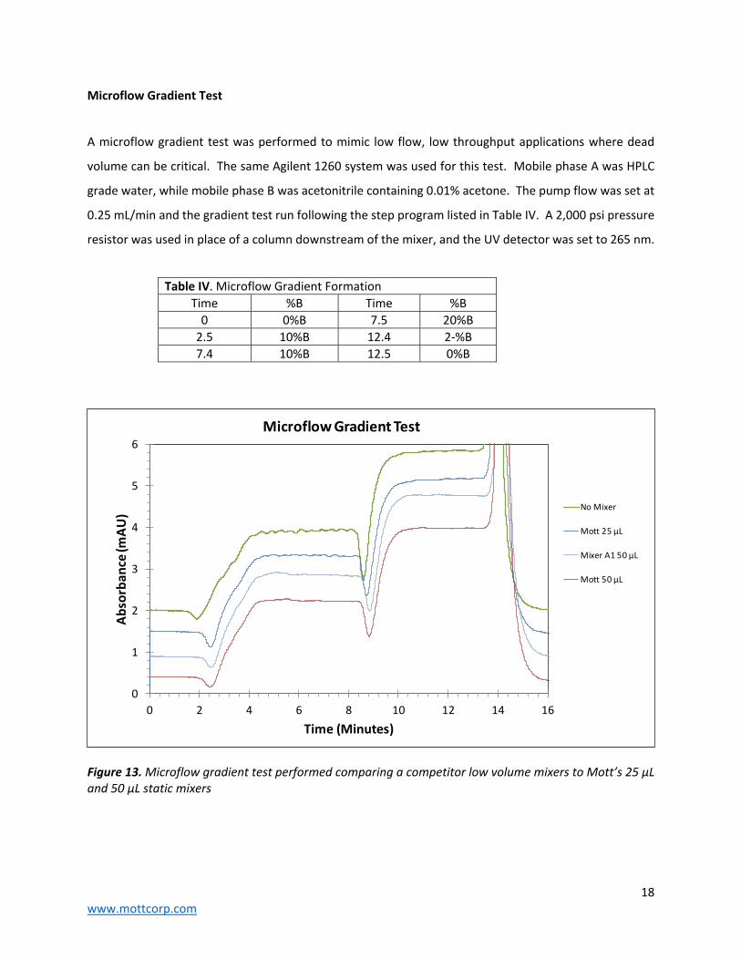
Microflow Gradient Test
A microflow gradient test was performed to mimic low flow, low throughput applications where dead
volume can be critical. The same Agilent 1260 system was used for this test. Mobile phase A was HPLC
grade water, while mobile phase B was acetonitrile containing 0.01% acetone. The pump flow was set at
0.25 mL/min and the gradient test run following the step program listed in Table IV. A 2,000 psi pressure
resistor was used in place of a column downstream of the mixer, and the UV detector was set to 265 nm.
Table IV. Microflow Gradient Formation
Time %B Time %B
0 0%B 7.5 20%B
2.5 10%B 12.4 2‐%B
7.4 10%B 12.5 0%B
Figure 13. Microflow gradient test performed comparing a competitor low volume mixers to Mott’s 25 µL and 50 µL static mixers
0
1
2
3
4
5
6
0 2 4 6 8 10 12 14 16
Absorban
ce (m
AU)
Time (Minutes)
Microflow Gradient Test
No Mixer
Mott 25 µL
Mixer A1 50 µL
Mott 50 µL
19 www.mottcorp.com
Presented in Figure 13 are gradient profiles for this test with no mixer installed, Mott’s 25 µL and 50 µL
mixers, and the competitor’s Mixer A1 50 µL. When the traces are examined for the Mott 50 µL and Mixer
A1 50 µL mixers, it can be seen they lag in time behind the others with no difference in their dwell times
(dip in traces near 9 minutes) indicating they have the same internal volumes. The Mott 25 µL mixer has
a shorter dwell time than both 50 µL mixers and is roughly midway between both 50 µL mixers and the
scan with no mixer installed. Less baseline ripple is also observed when mixers are installed with the Mott
25 µL and competitor’s Mixer A1 50 µL showing similar reductions in baseline ripple. The Mott 50 µL
mixer shows the lowest ripple amplitude of the mixers tested.
Summary
The recently developed line of patent‐pending Mott PerfectPeak® inline static mixers with five internal
volumes, 25 µL, 50 µL, 100 µL, 150 µL, and prototype 300 µL cover the range in volumes and mixing
performance needed for a majority of HPLC analyses, including difficult to mix gradients using TFA as an
additive, where enhanced mixing with low dispersion is required. The new static mixer accomplishes this
goal via use of a novel 3D printing technology to create a unique structure that achieves improved
hydrodynamic static mixing with the highest percentage reduction in baseline noise per unit of internal
mixture volume. Greater than 95% reduction in baseline noise was achieved using up to 1/2 the internal
volume of some commonly available mixers. This mixer consists of parallel and interconnected three‐
dimensional flow passageways that have varying cross‐sectional areas and path lengths as the fluid
transverses through and across internal complex geometric obstacles. The new line of static mixers
achieves improved performance over comparable competitors’ mixers, but with smaller internal volumes
and lower back pressures. This provides increased sensitivity through better signal to noise ratios and
lower limits of quantitation with improved peak shape, efficiency, and resolution even for difficult to mix
gradients employing TFA as an additive.
20 www.mottcorp.com
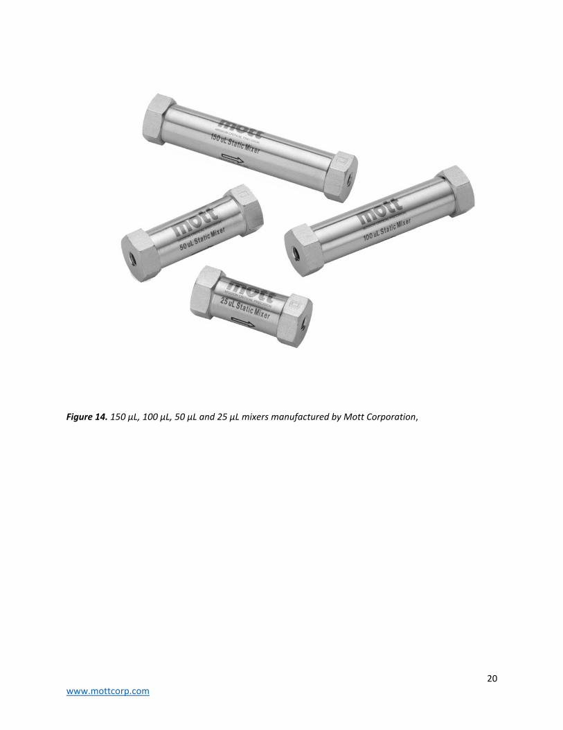
Figure 14. 150 µL, 100 µL, 50 µL and 25 µL mixers manufactured by Mott Corporation,

21 www.mottcorp.com
Mott Corporation, 84 Spring Lane, Farmington, CT 06032
www.mottcorp.com
860‐747‐6333


