
Proceedings of the 2016 International Conference on Industrial Engineering and Operations Management
Detroit, Michigan, USA, September 23-25, 2016
© IEOM Society International
Reliability Modeling for Rotor Systems with Imbalance
Based on Vibration Analysis
V. M. S. Hussain
Department of Manufacturing Engineering
National Institute of Foundry and Forge Technology
Hatia: Ranchi – 834003, India
V. N. A. Naikan
Reliability Engineering Center
Indian Institute of Technology
Kharagpur – 721 302, India.
Abstract
In Rotor systems, the imbalance fault generates high dynamic forces. These high dynamic forces are
catastrophic in nature at especially at high rotational speeds. This hypothesis is known to engineers,
but how it actually affects the reliability is not established. In this research work a vibration based
residual generation experimental method is proposed to relate imbalance in terms of vibration
amplitude and reliability. A stress-strength interference approach together with a simulation-based
methodology is used for modeling and analysis of this complex relationship. The paper also proposes
a method for establishing the safe and critical limits of imbalance and rotational speed for achieving
the specified reliability targets. Thus the concepts can be effectively used in industrial machinery for
controlling the level of imbalance of a rotor designed to operate at a specified rotational speed.
Keywords: Imbalance; Rotor systems; Reliability; Vibration analysis; Stress-Strength interference.
1. Introduction
During the operational stage of industrial rotor systems, the dynamic forces generated due to machinery faults
affect the system performance and reliability. The rotating machineries are vulnerable to varieties of defects and
faults such as mass imbalance, shaft misalignment, improper surface finish etc., which may lead to catastrophic
accidents [1]. Rotor imbalance is one of the most common faults and it generates unwanted motion of the rotors,
such as whirling and vibrations. A detailed literature survey on imbalance is presented in [2].
Many research works are available in the literature for identification and detection of faults in rotor systems. A
methodology for fault identification and diagnosis of machine faults based on the parameter estimation,
calculation of physical coefficients and symptom-fault tree is presented in [3, 4]. Model based fault
identification in the rotor systems is described by [5, 6]. The model based identification of faults for the
occurrence of two simultaneous faults (crack and imbalance) in the rotor system is presented by [7]. A model
based fault diagnosis of a rotor–bearing system is discussed in [8]. The authors identified faults such as
misalignment and imbalance using a test setup by comparing the experimental residual forces with theoretical
residual forces from fault models. Model based fault identification for the two imbalance faults in two-spin rotor
system is presented in [9]. An equivalent load minimization and vibration minimization method is applied for
identification of the imbalance [10]. The aforementioned literature shows that the vibration data of the system is
utilized by model based diagnostics to identify the commonly occurring faults such as imbalance, misalignment,
crack etc.
Many failure models for evaluating the reliability of the mechanical systems (viz rotor systems) are discussed in
[11]. Furthermore, this paper identifies that the Stress–Strength Interference (SSI) model is suitable for the
failure analysis of mechanical systems and components where strength and stress are often treated as the random
variables. A brief literature survey on SSI models and their applications is presented in [2, 12].
341
Proceedings of the 2016 International Conference on Industrial Engineering and Operations Management
Detroit, Michigan, USA, September 23-25, 2016
© IEOM Society International
The traditional approach for reliability assessment of the rotor systems is based on the factor of safety or safety
margin. This concept relies on the empirical methods and experience rather than statistical approach [13]. In
actual practice, it can be seen that the stress on a component and its strength are both random variables. For
example, the applied load on the rotor shaft is not a constant deterministic quantity. It depends on several factors
such as the variations in load, speed, friction and the additional forces due to imbalance, misalignment, etc.
Similarly, the strength of rotor shaft is also a function of several stochastic variables such as variations due to
manufacturing process, material strength, metal removal due to wear, corrosion, and other factors such as
fatigue. As we know, failure occurs when the stress on a component increases beyond its strength. Therefore,
the SSI models are found suitable for evaluating the reliability of the rotor systems subjected to the mass
imbalance.
A critical review of the literature indicated that some research work is available for reliability modeling of rotor
systems considering dynamic forces due to faults and defects. A theoretical model to relate reliability with mass
imbalance is presented in [2, 12]. However, experimental validation of such models is a very important step for
confirmation and acceptance of the models for practical applications in industry. This paper has presented a
frame work for carrying out such studies. The focus is on the most common problem of mass imbalance in rotor
systems and its effect on reliability. It is well known that the mass imbalance in rotor systems produces
additional centrifugal force and high vibration amplitude at rotational frequency. Therefore, an experimental
vibration analysis using a machine fault simulator and SSI approach has been used for developing a reliability
model for the rotor system with imbalance. Even though the current focus is only on the problem of imbalance,
the proposed frame work can be extended to include forces in rotor systems due to other faults such as
misalignment, resonance, oil whirl, etc.
The rest of this paper is organized as follows: Section 2 along with its sub sections present the various steps
followed for developing the proposed model. Section 3 illustrates the proposed model for the shaft of a rotor
system and the section 4 demonstrates proposed model for the shaft in an experimental setup with data
collection, analysis and interpretation of results. Section 5 presents the conclusions with scope of future work.
The paper ends with references.
2. Proposed Reliability Model The force due to imbalance in a rotor system depends on the amount of imbalance mass, its distance from the
axis of rotation, and the rotational speed [14]. The force produced due to imbalance is given by,
𝐹𝑖𝑚 = 𝑚𝑟𝜔2 (1)
From the equation (1), it can be found that a small amount of imbalance mass will generate huge force resulting
in substantial amount of stress on the system.
In Industrial rotor systems, it is difficult to estimate the amount of imbalance mass and its distance from the axis
of rotation, and hence the equation (1) will be only of theoretical importance. Hence, the residual force
generation technique of model based diagnosis which is discussed in [5, 6, 8, 9, 10] is used to estimate the
amount of force due to imbalance mass in the practical rotor systems. The model presented here uses the
information of a dynamic model of rotor system, and it uses the difference between the vibration response of the
rotor system with fault and without fault conditions.
2.1 Residual Force Generation The vibrations of an undamaged rotor system represented by the displacement vector 𝐱𝑜(𝑡) at N degrees of
freedom due to the operating load 𝐅𝑜(𝑡) during normal operating condition is described by the linear equation of
motion (2),
𝐌�̈�0(𝑡) + 𝐂�̇�𝑜(𝑡) + 𝐊𝐱𝑜(𝑡) = 𝐅𝑜(𝑡) (2)
The occurrence of a fault in the undamaged system induces the change in the dynamic behavior of the system.
The change in dynamic behavior depends on the type of fault, severity of the fault and location of its occurrence.
The introduction of the fault in the undamaged system adds the additional load and influences the change in the
vibration response. The equation of motion for the faulty system is represented by,
𝐌�̈�(𝑡) + 𝐂�̇�(𝑡) + 𝐊𝐱(𝑡) = 𝐅𝑜(𝑡) + ∆𝐅(𝑡) (3)
The difference between the faultless system response and the faulty system response will give the residual
displacements, velocities and accelerations. These are represented as,
∆𝐱(𝑡) = 𝐱(𝑡) − 𝐱𝑜(𝑡) (4)
∆�̇�(𝑡) = �̇�(𝑡) − �̇�𝑜(𝑡) (5)
∆�̈�(𝑡) = �̈�(𝑡) − �̈�𝑜(𝑡) (6)
342
Proceedings of the 2016 International Conference on Industrial Engineering and Operations Management
Detroit, Michigan, USA, September 23-25, 2016
© IEOM Society International
The subtraction of equation of motion of undamaged system (2) from the equation of motion of the faulty
system (3) and substituting (4, 5 and 6) yields the following equation,
𝐌∆�̈�(𝑡) + 𝐂∆�̇�(𝑡) + 𝐊∆𝐱(𝑡) = ∆𝐅(𝑡) (7)
In this model it is assumed that the rotor system is linear and hence the system matrices (M, C, and K) remain
unchanged. The equivalent load represented as ∆𝐅(𝑡) induces the change in the dynamic behavior of the
undamaged linear rotor system and this equivalent load will fetch the magnitude of the fault and the location of
its occurrence. This additional force (∆𝐅(𝑡)) due to fault is also termed as residual force.
To calculate the residual vibration response due to the fault in the rotor system, the measured vibration response
data for both undamaged and faulty rotor system should be available for the same operating and measurement
conditions [5, 7, 8, 15].
2.2 Modal expansion To compute the residual force vector (∆𝐅(𝑡)) at all the nodes, the residual vibration response at all the degrees
of freedom (N) of the system should be available in the form of residual displacement, residual velocity and
residual acceleration. But due to the practical limitations, the vibration response is measured only in few degrees
of freedom (𝑛) and hence 𝑛 ≪ 𝑁.
The vibration response for the non-measurable degrees of freedom has to be estimated from the measured
vibration response. To estimate the residual vibration at all degrees of freedom from the measured residual
vibration response ∆𝐱n(𝑡), the modal expansion technique is used. This modal expansion technique is rooted on
the approximation of the residual vibration by a linear combination of few eigenvectors (�̂�). The full residual
vector ∆𝐱(𝑡) can be approximated by a reduced modal matrix �̂� which contain a set of mode shapes �̂�k
�̂� = [�̂�1, �̂�2, . . . �̂�k] (9)
The number of mode shapes used in the reduced modal matrix �̂� , logically may not exceed the number of
independently measured vibration response contained in the ∆𝐱n(𝑡), i.e. 𝐾 ≤ 𝑛.
Now, the measured residual vibration response ∆𝐱n(𝑡) is related to the full residual vector ∆𝐱(𝑡) by the
transformation matrix �̃� , which uses the modal matrix �̂�, and given by
∆𝐱n(𝑡) = �̃� ∆𝐱(𝑡) (8)
In this research paper, for the expansion of the available measured data ∆𝐱n(𝑡) the System Equivalent
Reduction Expansion Process (SEREP) has been used. The SEREP expansion technique utilizes the SEREP
transformation matrix to expand the measured degrees of freedom in all the degrees of the system [16]. The
SEREP transformation matrix is given by
�̃� = [𝜙][�̂�]𝑔
(9)
where
[�̂�]𝑔
= [[�̂�]𝑇
[�̂�]]−1
[�̂�]𝑇
(10)
2.3 Residual Force The residual force ∆𝐅(𝑡) which characterizes the fault is calculated by substituting the system matrices which
describes the system mass, damping and stiffness, and the residual vibration response of the full vibration state
in the form of residual displacement, residual velocity and residual acceleration, in the equation (7). And the
corresponding substitution of equation (8) finally yields the equation (11),
𝐌�̃�∆�̈�n(𝑡) + 𝐂�̃�∆�̇�n(𝑡) + 𝐊�̃�∆𝐱n(𝑡) = ∆𝐅(𝑡) (11)
The equation (11) can be used to estimate the equivalent loads at all the degrees of freedom from the few
measured vibration responses.
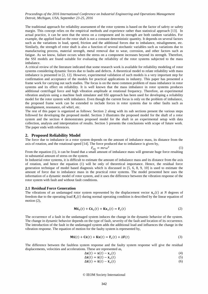
2.4 Effective stress The force due to imbalance (𝐹𝑖𝑚) has to be found from the vector of equivalent load (∆𝐅(𝑡)). The force due to
imbalance is accountable for the additional stress in the system, apart from the design stress. The imbalance
force is used to compute equivalent additional stress. This additional stress is to be incorporated in to the design
equation of the system, to find the effective stress. The effective stress is used to find the reliability of the
system. This procedure of finding effective stress has been shown in Figure 2. Following sub-section explains
about the reliability computation using the effective stress in the component and the ultimate strength of the
component.
343

Proceedings of the 2016 International Conference on Industrial Engineering and Operations Management
Detroit, Michigan, USA, September 23-25, 2016
© IEOM Society International
2.5 Reliability modeling for imbalance To calculate the reliability of the rotor system the stress-strength interference (SSI) failure model is used [11,
16]. For this SSI failure model, the following reliability expression (12) has been used. Equation (12) represents
the reliability of the component or system for all the possible values of strength (𝑆𝑇𝐻) of the component and
stress (𝑆𝑡𝑠) on the component.
𝑅 = ∫ 𝑓𝑆𝑇𝐻
∞
−∞
(𝑆𝑇𝐻) [ ∫ 𝑓𝑆𝑡𝑠(𝑆𝑡𝑠)
𝑆𝑇𝐻
−∞
d𝑆𝑡𝑠] d𝑆𝑇𝐻 (12)
The proposed model has been shown in the form of flowchart in figure 1 and it is illustrated by a numerical
example in the following section.
3. Illustration for the Proposed Reliability Model for a Shaft
The shaft element of rotor system has been considered here for the illustration. The design equation of the shaft
is used to find the effective stress in the shaft. The Guest’s and Rankine’s shaft design equations (13, 14) are
used to estimate the design stress [18]. It is suggested that design stress may be obtained by using both the
theories (13, 14) and the larger of the two values is adopted for designing the shaft [18].
𝜏𝑚𝑎𝑥 =16√𝑀𝑏
2+𝑇2
𝜋𝑑3 (13)
𝜎𝑚𝑎𝑥 =
32 (𝑀𝑏 + √𝑀𝑏
2 + 𝑇2
2)
𝜋𝑑3
(14)
The addition of bending moment (𝑀𝑖𝑚) due to imbalance force (𝐹𝑖𝑚) in the stress equations (13, 14) will lead to
the effective stress equation. The effective stress equations for shaft based on the maximum shear stress and
maximum normal stress are given in equations (15, 16).
𝜏𝑒𝑓𝑓 =16√(𝑀𝑖𝑚 + 𝑀𝑏)2 + 𝑇2
𝜋𝑑3
(15)
𝜎𝑒𝑓𝑓 =
32 ((𝑀𝑖𝑚 + 𝑀𝑏)2 + √(𝑀𝑖𝑚 + 𝑀𝑏)2 + 𝑇2
2)
𝜋𝑑3
(16)
The effective stress equations (15, 16) will estimate the total stress in the shaft, including the stress produced
due to imbalance force.
The effective stress equations (15, 16) of any mechanical component or system will have variables which are
probabilistic in nature, rather than deterministic. This randomness makes the reliability calculations difficult and
complex. To calculate the reliability of the component with such randomness, we require large amount of field
test data to compute the stresses accurately. This is not practically feasible. Therefore, the simulation technique
is used to generate and compute the stresses. For example, in the equations (15, 16), variables such as, radius of
shaft, length of the shaft, ultimate tensile stress and ultimate normal stresses are probabilistic in nature. The
arbitrariness in the aforementioned variables are due to many reasons such as, manufacturing variations while
metal working or casting etc., heat treatment variations, dimensional errors due to human or machine
inaccuracy, power fluctuations, environmental effects, etc.
The random variables, such as the radius of the shaft, ultimate tensile stress, and ultimate normal stress will
exhibit arbitrariness. To theoretically calculate the reliability for a shaft, the generation of random variables
representing the arbitrariness of the radius of the shaft, ultimate tensile and normal stresses according to their
probabilistic characteristics is necessary. For this, random numbers (distributed between 0 and 1) are generated
using a computer program. These random numbers are used to generate the values for random variables to
represent the probabilistic nature of the variables. The generation of random numbers and generation of
continuous and discrete random variables using random numbers are discussed in [19].
The generation of continuous random variable according to their probabilistic nature and the calculation for each
realization of random variable in equations (15, 16) will give a probabilistic character for the effective stress.
And in the same way the ultimate shear strength and ultimate normal strength for the shaft with a particular
material type and shape is generated according to their probabilistic characters. This ultimate shear strength and
344

Proceedings of the 2016 International Conference on Industrial Engineering and Operations Management
Detroit, Michigan, USA, September 23-25, 2016
© IEOM Society International
ultimate normal strength will resist the effective shear stresses and effective normal stresses acting on the shaft. The SSI equation [17] for the maximum shear stress model and maximum normal stress model are given in the
following equations (17, 18) respectively,
𝑅 = ∫ 𝑓𝜍
∞
−∞
(𝜍) [ ∫ 𝑓𝜎𝑒𝑓𝑓(𝜎𝑒𝑓𝑓)
𝜍
−∞
d𝜎𝑒𝑓𝑓] d𝜍 (17)
𝑅 = ∫ 𝑓𝒯
∞
−∞
(𝒯) [ ∫ 𝑓𝜏𝑒𝑓𝑓(𝜏𝑒𝑓𝑓)
𝒯
−∞
d𝜏𝑒𝑓𝑓] d𝒯 (18)
Figure 1: Flow chart of the proposed reliability model for rotor system with imbalance fault
After the simulation cycles (in this illustration 250,000 simulation cycles) the resultant random variables for the
τeff and σeff are fit into the suitable distribution. A similar procedure is followed for generation of the strength
variables. Reliability of the shaft is computed by substituting the density functions and its parameters in the
345
Proceedings of the 2016 International Conference on Industrial Engineering and Operations Management
Detroit, Michigan, USA, September 23-25, 2016
© IEOM Society International
equations (17, 18). An experimental method is used to physically simulate imbalance and to measure the
vibration due to this. The stresses are computed based on the measured vibrations.
Figure 2: Flow chart for computation of effective stress
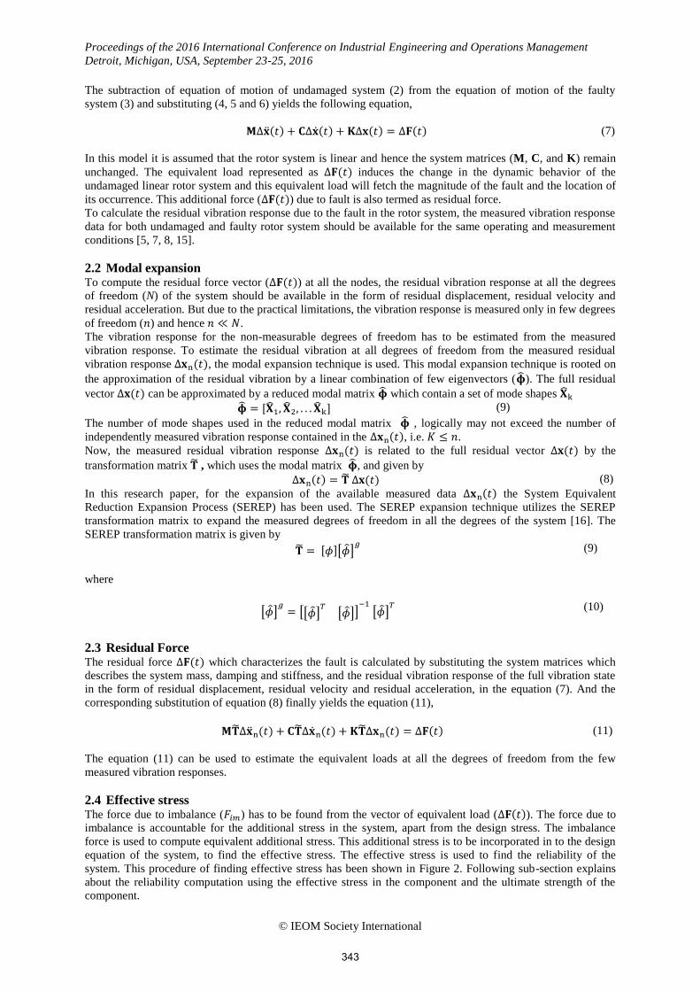
4. Experimental work for the illustration The experimental work to get acquire the vibration response is carried out in a machine fault simulator (MFS)
test rig. The fault simulator is having provisions to introduce different types of faults to carry out the
experimental work. The finite element modeling [20] of the test setup has been given in the appendix-I. The
schematic diagram of the MFS with the essential dimensions, and the photograph has been shown in figure 3.
Four ICP accelerometers (0.3 – 10 KHz, 100m V/G) with BNC connectors are used for vibration data
acquisition. The OROS software is used to acquire and investigate vibration data. The OROS uses the digital
integration to find the displacement and velocity amplitude from the measured acceleration data, and OriginPro
is used to plot the data. MATLAB software has been used to write codes for the further analysis of the acquired
data.
Figure 3:Schematic representation of experimental setup Figure 4: Finite element model of test setup
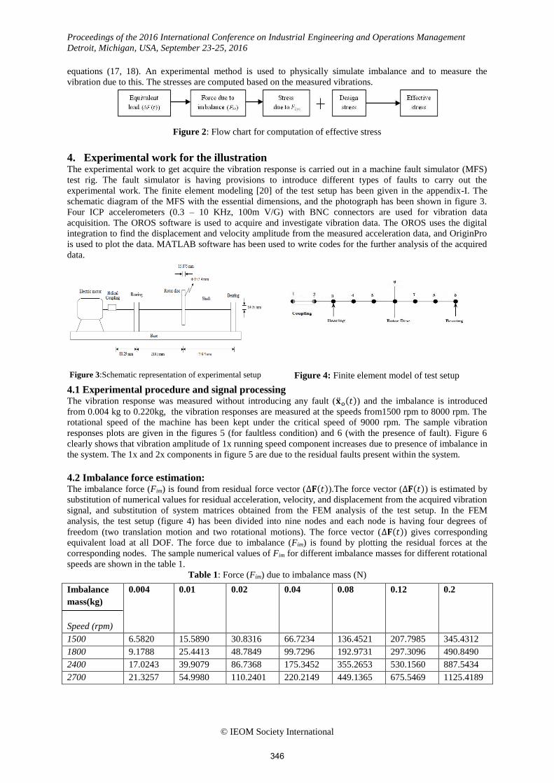
4.1 Experimental procedure and signal processing The vibration response was measured without introducing any fault (�̈�o(𝑡)) and the imbalance is introduced
from 0.004 kg to 0.220kg, the vibration responses are measured at the speeds from1500 rpm to 8000 rpm. The
rotational speed of the machine has been kept under the critical speed of 9000 rpm. The sample vibration
responses plots are given in the figures 5 (for faultless condition) and 6 (with the presence of fault). Figure 6
clearly shows that vibration amplitude of 1x running speed component increases due to presence of imbalance in
the system. The 1x and 2x components in figure 5 are due to the residual faults present within the system.
4.2 Imbalance force estimation: The imbalance force (Fim) is found from residual force vector (∆𝐅(𝑡)).The force vector (∆𝐅(𝑡)) is estimated by
substitution of numerical values for residual acceleration, velocity, and displacement from the acquired vibration
signal, and substitution of system matrices obtained from the FEM analysis of the test setup. In the FEM
analysis, the test setup (figure 4) has been divided into nine nodes and each node is having four degrees of
freedom (two translation motion and two rotational motions). The force vector (∆𝐅(𝑡)) gives corresponding
equivalent load at all DOF. The force due to imbalance (Fim) is found by plotting the residual forces at the
corresponding nodes. The sample numerical values of Fim for different imbalance masses for different rotational
speeds are shown in the table 1.
Table 1: Force (Fim) due to imbalance mass (N)
Imbalance
mass(kg)
Speed (rpm)
0.004 0.01 0.02 0.04 0.08 0.12 0.2
1500 6.5820 15.5890 30.8316 66.7234 136.4521 207.7985 345.4312
1800 9.1788 25.4413 48.7849 99.7296 192.9731 297.3096 490.8490
2400 17.0243 39.9079 86.7368 175.3452 355.2653 530.1560 887.5434
2700 21.3257 54.9980 110.2401 220.2149 449.1365 675.5469 1125.4189
346
Proceedings of the 2016 International Conference on Industrial Engineering and Operations Management
Detroit, Michigan, USA, September 23-25, 2016
© IEOM Society International
4.3 Reliability Estimation: The numerical values of force due to imbalance are used to compute the additional bending moment in the shaft,
as explained in sub-section 2.4. The required values of different parameters and additional bending moment are
substituted in the equations (15, 16) to get the effective stress values. The shear stress (τeff) and the ultimate
shear strength (𝒯) values obtained after the simulation cycles follow the standard normal distribution.
Substitution of the normal distribution density functions of stress and strength in the Eq. (18) the following
reliability expression (19) is obtained [17]. By substituting the parameters of the distributions in equation (19)
reliability of the shaft is computed.
𝑅 = 1 − 𝛷(𝑧) (19)
where 𝑧 = (𝜇𝒯− 𝜇𝜏𝑒𝑓𝑓
)
√(𝜚𝒯)2+(𝜚𝜏𝑒𝑓𝑓)2
(a)
(b)
Figure 5: Vibration response at 25 Hz without imbalance mass (a) Time domain (b) Frequency domain
(a)
(b)
Figure 6: Vibration response at 25 Hz with imbalance mass 0.004kg (a) Time domain (b) Frequency domain
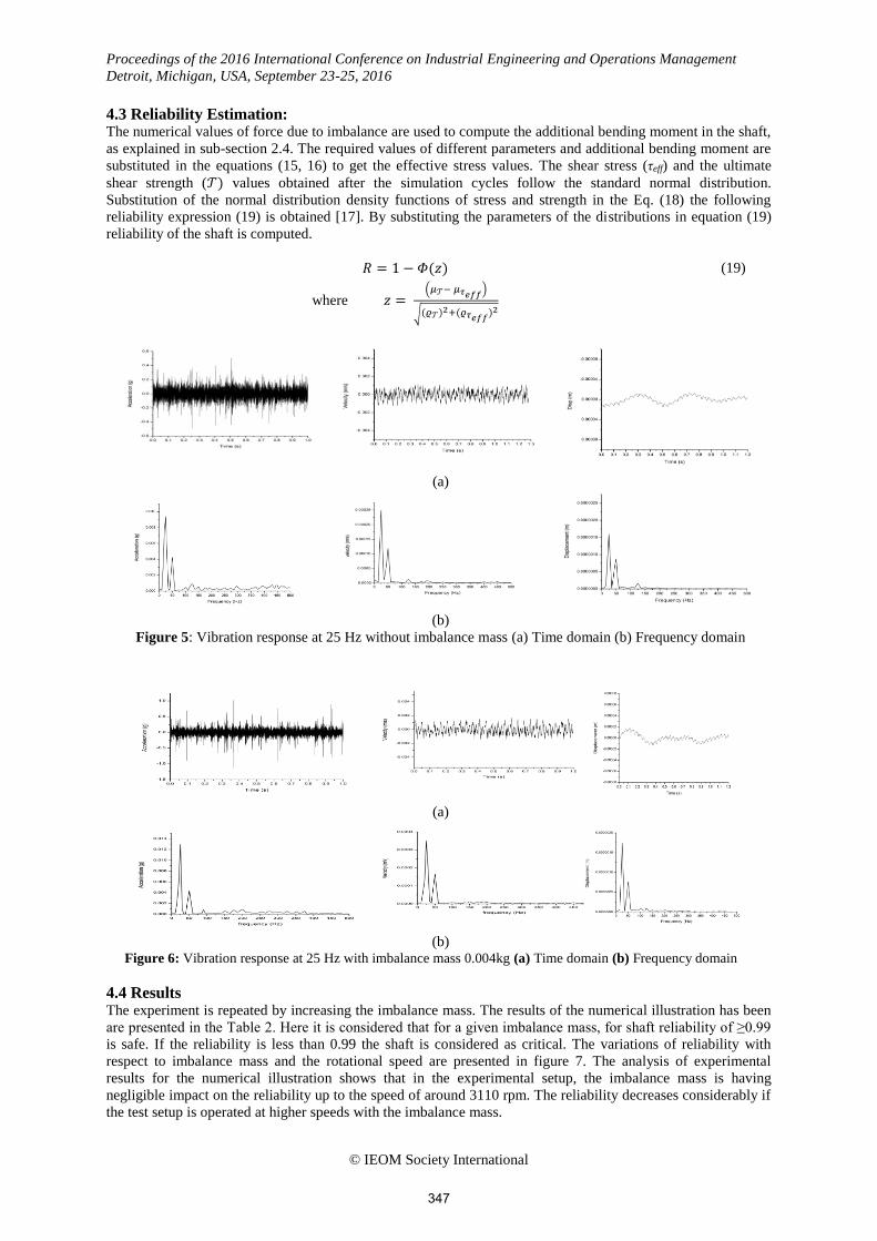
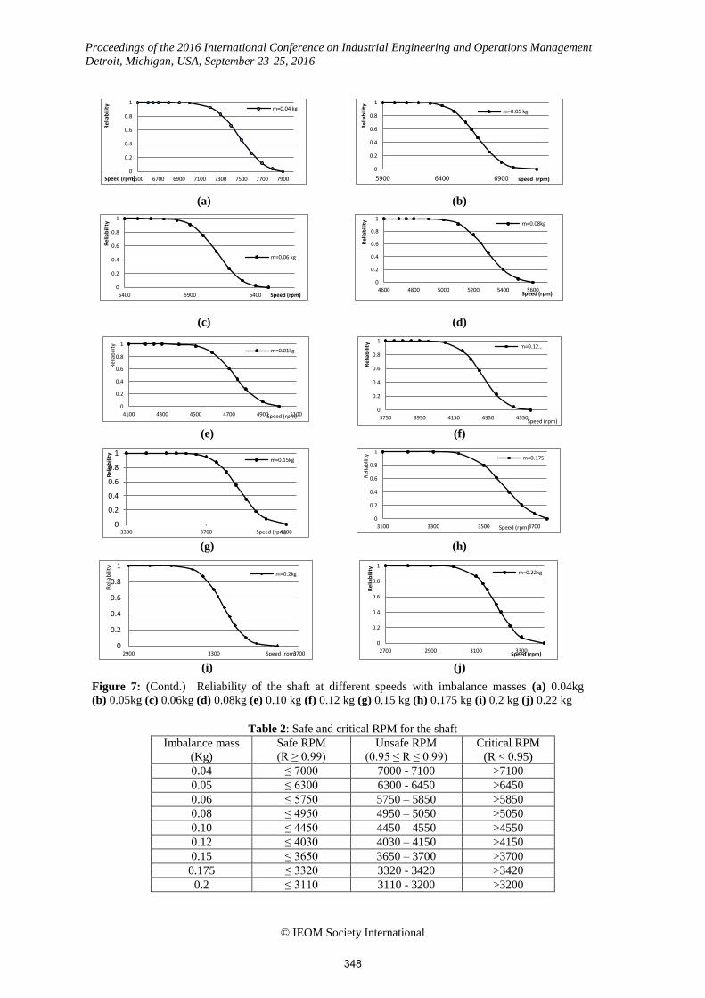
4.4 Results The experiment is repeated by increasing the imbalance mass. The results of the numerical illustration has been
are presented in the Table 2. Here it is considered that for a given imbalance mass, for shaft reliability of ≥0.99
is safe. If the reliability is less than 0.99 the shaft is considered as critical. The variations of reliability with
respect to imbalance mass and the rotational speed are presented in figure 7. The analysis of experimental
results for the numerical illustration shows that in the experimental setup, the imbalance mass is having
negligible impact on the reliability up to the speed of around 3110 rpm. The reliability decreases considerably if
the test setup is operated at higher speeds with the imbalance mass.
347
Proceedings of the 2016 International Conference on Industrial Engineering and Operations Management
Detroit, Michigan, USA, September 23-25, 2016
© IEOM Society International
(a)
(b)
(c)
(d)
(e)
(f)
(g)
(h)
(i)
(j)
Figure 7: (Contd.) Reliability of the shaft at different speeds with imbalance masses (a) 0.04kg
(b) 0.05kg (c) 0.06kg (d) 0.08kg (e) 0.10 kg (f) 0.12 kg (g) 0.15 kg (h) 0.175 kg (i) 0.2 kg (j) 0.22 kg
Table 2: Safe and critical RPM for the shaft
Imbalance mass
(Kg)
Safe RPM
(R ≥ 0.99)
Unsafe RPM
(0.95 ≤ R ≤ 0.99)
Critical RPM
(R < 0.95)
0.04 ≤ 7000 7000 - 7100 >7100
0.05 ≤ 6300 6300 - 6450 >6450
0.06 ≤ 5750 5750 – 5850 >5850
0.08 ≤ 4950 4950 – 5050 >5050
0.10 ≤ 4450 4450 – 4550 >4550
0.12 ≤ 4030 4030 – 4150 >4150
0.15 ≤ 3650 3650 – 3700 >3700
0.175 ≤ 3320 3320 - 3420 >3420
0.2 ≤ 3110 3110 - 3200 >3200
0
0.2
0.4
0.6
0.8
1
6500 6700 6900 7100 7300 7500 7700 7900
Rel
iab
ility
Speed (rpm)
m=0.04 kg
0
0.2
0.4
0.6
0.8
1
5900 6400 6900
Rel
iab
ility
speed (rpm)
m=0.05 kg
0
0.2
0.4
0.6
0.8
1
5400 5900 6400
Rel
iab
ility
Speed (rpm)
m=0.06 kg
0
0.2
0.4
0.6
0.8
1
4600 4800 5000 5200 5400 5600
Rel
iab
ility
Speed (rpm)
m=0.08kg
0
0.2
0.4
0.6
0.8
1
4100 4300 4500 4700 4900 5100
Rel
iab
ility
Speed (rpm)
m=0.01kg
0
0.2
0.4
0.6
0.8
1
3750 3950 4150 4350 4550
Rel
iab
ility
Speed (rpm)
m=0.12…
0
0.2
0.4
0.6
0.8
1
3300 3700 4100
Re
liab
ility
Speed (rpm)
m=0.15kg
0
0.2
0.4
0.6
0.8
1
3100 3300 3500 3700
Rel
iab
ility
Speed (rpm)
m=0.175
0
0.2
0.4
0.6
0.8
1
2900 3300 3700
Rel
iab
ility
Speed (rpm)
m=0.2kg
0
0.2
0.4
0.6
0.8
1
2700 2900 3100 3300
Re
liab
ility
Speed (rpm)
m=0.22kg
348

Proceedings of the 2016 International Conference on Industrial Engineering and Operations Management
Detroit, Michigan, USA, September 23-25, 2016
© IEOM Society International
If the imbalance mass can be limited by regular monitoring and correction, then the system can be highly
reliable and safe to operate at higher speeds. Therefore it is suggested that this system needs periodic monitoring
and balancing.
5. Conclusions Imbalance in rotating systems results in huge dynamic forces at higher rotational speeds, leading to failure and
catastrophic accidents. In this research work, a reliability model based on the experimental methodology has
been presented and illustrated with an example. The model can be effectively used to predict the operational
reliability of rotor systems with imbalance, by measuring their vibration amplitude. If the reliability target is
specified, safe ranges of operational speed can be established for an existing or new system using this model.
The model presented in this research work will have practical application in the areas of safety and reliability in
the aviation sector, power generating equipment and could even be applied in surface transport and shipping
where huge propellers and gear boxes are used. As future scope, new reliability models may be developed based
on experimental methodology for the rotor system faults such as misalignment, and oil whirl.
Notation: 𝐹𝑖𝑚 : Force due to imbalance
𝑚 : Imbalance mass
𝑟 : Distance between imbalance mass and the axis of rotation
𝜔 : Angular velocity of shaft
𝐌 : Mass matrix
𝐂 : Damping matrix
𝐊 : Stiffness matrix
�̈�0(𝑡) : Acceleration vector of faultless rotor system
�̇�𝑜(𝑡) : Velocity vector of faultless rotor system
𝐱𝑜(𝑡) : Displacement vector of faultless rotor system
𝐅𝑜(𝑡) : Force vector of faultless rotor system
�̈�(𝑡) : Acceleration vector of faulty rotor system
�̇�(𝑡) : Velocity vector of faulty rotor system
𝐱(𝑡) : Displacement vector of faulty rotor system
∆𝐅(𝑡) : Equivalent load vector
𝑛 : Measurable degrees of freedom
𝑁 : Degrees of freedom
∆𝐱𝑛(𝑡) : Measured residual vector
�̃� : Transformation matrix
∆𝐱(𝑡) : Residual displacement vector
∆�̇�(𝑡) : Residual velocity vector
∆�̈�(𝑡) : Residual acceleration vector
�̂� : Reduced modal matrix
�̂�1, �̂�2, . . . �̂�𝑘 : Mode shapes
∆𝐪(𝑡) : Modal coordinate vector
𝑅 : Reliability
𝑆𝑡𝑠 : Stress in the shaft
𝑆𝑇𝐻 : Strength of the shaft
𝑓𝑆𝑡𝑠(𝑆𝑡𝑠) : Probability density function of stress
𝑓𝑆𝑇𝐻(𝑆𝑇𝐻) : Probability density function of strength
τmax : Maximum shear stress
Mb Bending moment
T : Torque
d : Cross sectional diameter of shaft
𝜎max : Maximum bending stress
τeff : Effective shear stress
Mim : Bending moment due to imbalance force
𝜎eff : Effective bending stress
𝒯 : Ultimate shear strength
ς : Ultimate normal strength
𝑓𝜍(𝜍) : Density function of ultimate normal strength
𝑓𝒯(𝒯) : Density function of ultimate shear strength
𝑓𝜏𝑒𝑓𝑓(𝜏𝑒𝑓𝑓) : Density function of effective shear stress
349

Proceedings of the 2016 International Conference on Industrial Engineering and Operations Management
Detroit, Michigan, USA, September 23-25, 2016
© IEOM Society International
𝑓𝜎𝑒𝑓𝑓(𝜎𝑒𝑓𝑓) : Density function of effective normal stress
𝛷(𝑧) : Standard cumulative normal distribution function
𝜇𝒯 : Mean of ultimate shear strength
𝜚𝒯 : Standard distribution of ultimate shear strength
𝜇𝜏𝑒𝑓𝑓 : Mean of effective shear strength
𝜚𝜏𝑒𝑓𝑓 : Standard distribution of effective shear strength
[ ]𝑇 : Transpose
References 1. Othman, N.A., N.S. Damanhuri, and V. Kadirkamanathan, The Study of Fault Diagnosis in Rotating
Machinery. Proceedings of 5th International Colloquium on Signal Processing and Its Applications, Kuala
Lumpur, Malaysia, March 2009, 69-74
2. Hussain, V.M.S. and V.N.A. Naikan, Reliability and Imbalance Modeling of a Low Pressure Turbine
Rotor. International Journal of Life Cycle Reliability and Safety Engineering, 1 (2), 2012, 61-70.
3. Isermann, R., M. Ayoubi, H. Konrad and T.Reiss, Model Based Detection of Tool Wear and Breakage for
Machine Tools. Proceedings of the IEEE International Conference on Systems, Man and Cybernetics,
Volume 3, Le Touquet, France, 1993, 72-77. doi: 10.1109/ICSMC.1993.384988
4. Iserman, R., Model Based Fault Detection and Diagnosis Methods. Proceedings of the American control
Conference, Seattle, Washington, June 1995, 1605-1609.
5. Markert, R., R. Platz, and M. Seidler, Model Based Fault Identification in Rotor Systems by Least Squares
Fitting. International Journal of Rotating Machinery, 7 (5), 200, 311-321.
6. Bachschmid, N., P. Pennacchi, A. Vania, L. Gregori, and G.A. Zanetta, Unbalance Identification in a
Large Steam Turbo Generator Using Model-Based Identification and Modal Foundation. Proceedings of
the 8th International Conference on Vibrations in Rotating Machinery, IMechE, Swansea, 2004, 383-392.
7. Sekhar, A.S., Identification of Unbalance and Crack Acting Simultaneously in a Rotor System: Modal
Expansion Versus Reduced Basis Dynamic Expansion. Journal of Vibration and Control, 11 (9), 2005,
1125-1145. doi:10.1177/1077546305042531
8. Jalan, A.k., and A.R. Mohanty, Model Based Fault Diagnosis of a Rotor-Bearing System for Misalignment
and Unbalance under Steady-State Condition. Journal of Sound and Vibration, 327, 2009, 604-622. doi:
10.1016/j.jsv.2019.07.014
9. Luo,Y.G., S.H. Zhang, H.L. Yao, and B.C. Wen, Application of Model Based Diagnosis in Two-Span
Rotor System with Two Unbalance Faults. Advanced Materials Research, 199-200, 2011, 780-783
10. Sudhakar, G.N.D.S., and A.S. Sekhar, Identification of Unbalance in a Rotor Bearing System. Journal of
Sound and Vibration, 330, 2011, 2299-2313. doi:10.1016/j.jsv.2010.11.028
11. Dasgupta, A., and M. Pecht, Material Failure Mechanisms and Damage Models. IEEE Transactions on
Reliability, 40 (5), 1991, 531-536.
12. Hussain, V.M.S., and V.N.A. Naikan, Reliability Modeling of Rotor systems Subjected to Imbalance.
International Journal of Performability Engineering, 9 (4), 2013, 423-432.
13. Carter, A.D.S., Mechanical Reliability and Design. McMillan, Hong Kong, 1997.
14. Collacott, R.A., Vibration Monitoring and Diagnosis. John Willey, New York, 1979
15. Platz, R., and R. Markert, Fault Models for On-line Identification of Malfunctions in Rotor System.
Transactions of Fourth International Conference on Acoustical and Vibratory Surveillance, Senlis, France,
2001, 435–446.
16. Pingle P, Avitabile P. Prediction of full field dynamic stress/strain from limited sets of measured data,
Structural Dynamics, Volume 3. Springer, New York, 2011
17. Kapoor, K.C., and L.R. Lamberson, Reliability in Engineering Design. John Willey, New York, 1997.
18. Kurmi, R.S., and J.K. Gupta, A Text Book on Machine Design. Eurasia publishing House Ltd., New Delhi,
2005.
19. Halder, A., and S. Mahadevan, Reliability Assessment Using Stochastic Finite Element Analysis. John
Wiley, New York, 2000.
20. Nelson, H.D., and J.M. McVaugh, The Dynamics of Rotor-Bearing Systems Using Finite Elements.
Transactions of ASME - Journal of Engineering for Industry, 98 (2), 1976, 593-600. Vallayil N. A. Naikan is a professor and head of the Reliability Engineering Center Indian Institute of
Technology, Kharagpur. He obtained his M.Tech. and Ph.D. in the reliability engineering from Reliability
Engineering Center Indian Institute of Technology, Kharagpur. He has authored several research papers and
books. His area of research includes mechanical system reliability, SPC, system dynamics simulation, and fault
diagnosis. He has experience in working with University of Maryland, USA, the Chinese University of Hong
350

Proceedings of the 2016 International Conference on Industrial Engineering and Operations Management
Detroit, Michigan, USA, September 23-25, 2016
© IEOM Society International
Kong, Indian Space Research Organization, IIM, Ahmedabad and Union Carbide Calcutta. He is member of
several professional societies and in the editorial board of several reputed research journals.
V. M. S. Hussain is an Assistant Professor in National Institute of Foundry and Forge Technology, Ranchi. He
is a graduate from Vellore Institute of Technology (under University of Madras) with the specialization of
Mechanical engineering. He obtained his M. Engg. (Production Engineering) from FEAT, Annamalai
University. Currently, he is working for his Ph.D., in Reliability Engineering Center, Indian Institute of
Technology, Kharagpur.
Appendix I Modeling of test setup:
The FEM formulation of Nelson and McVaugh [20] is used to model the rotor system to get the system matrices
(M, C, and K). Here the equation of motion for the interconnected rotor, shaft and bearing has been presented; it
is considered here that, four degrees of freedom, two translation motions in horizontal (W) and vertical (V)
directions, and two rotational motions about horizontal (𝜃𝑊 ) and vertical (𝜃𝑉) axes, respectively at each node.
The shaft is divided into nine elements, using the finite element method and using the Lagrangian formulation,
the equation of motion for the shaft element presented by Nelson et al [20]. The Lagrangian equation of motion
of the finite shaft element with the constant rotational speed is given by
(𝐌𝑇𝑒 + 𝐌𝑅
𝑒 )�̈�𝑒 − Ω𝐆𝑒�̇�𝑒 + (𝐊𝐵𝑒 + 𝐊𝐴
𝑒)𝐱𝑒 = 𝐅𝑒
where {𝐱}𝑇 = [𝑊 𝑉 𝜃𝑊 𝜃𝑉] (A.1)
The force vector {𝐅𝑒} include mass imbalance, interconnection forces and other element external effects. In
appendix the individual element matrices are listed.
The Lagrangian equation of motion of the rigid disk with four DOF as discussed for the shaft element, with
the constant rotational speed (Ω) is given by Nelson et al [20]
(𝐌𝑇𝑑 + 𝐌𝑅
𝑑)�̈�𝑑 − Ω𝐆𝑑�̇�𝑑 = 𝐅𝑑 (A.2)
The vector 𝐅𝑑 represents the force which includes the mass imbalance, interconnection forces and other external
forces on the rotor. In appendix the individual rotor matrices are listed.
In this test set up the anti-friction bearings are used and the general equation of motion for the bearings is
given by
𝐂𝑏�̇�𝑏 + 𝐊𝑏𝐱𝑏 = 𝐅𝑏
where 𝐱𝑏 = {𝑊𝑉
}, 𝐊𝑏 = [𝑘𝑊𝑊
𝑏 𝑘𝑊𝑉𝑏
𝑘𝑉𝑊𝑏 𝑘𝑉𝑉
𝑏 ], 𝐂𝑏 = [𝑐𝑊𝑊
𝑏 𝑐𝑊𝑉𝑏
𝑐𝑉𝑊𝑏 𝑐𝑉𝑉
𝑏 ]
(A.3)
and {𝐅𝑏} is the external force vector on the bearings given by [20].
For the isotropic bearings which are used in this present study represented by the following equation,
𝑐[𝐈]�̇�𝑅𝑏 + 𝑘[𝐈]𝐱𝑅
𝑏 = 𝐅 ́𝑏 (A.4)
Where c and k are the isotropic bearing damping and stiffness coefficient respectively, and 𝐅 ́𝑏 and 𝐱𝑅𝑏 are the
external force vector relative to the rotational reference frame [20]. For further detailed study on the modeling of
rotor bearing system based on finite elements [20] can be referred.
The final assembled equation of motion of the rotor system of the test rig will be given in the following
equation as,
𝐌�̈� + 𝐂�̇� + 𝐊𝐱 = 𝐅 (A.5)
Where the M is the mass matrix and it consist of translational and rotor mass matrices of shaft elements and the
rotor, C includes gyroscopic moments and damping of bearings, and K is the stiffness matrix and it includes
shaft element stiffness and bearing stiffness. The force matrix F includes the weight of the disk, force due to
imbalance at constant rotational speed, bearing force, and other external force if any. For the elemental matrices
of the rotor system [8, 10, 20] can be referred.
351


