
WORKING PAPER
REPAIRING THE MIGRATION DATA REPORTED BY THE AMERICAN COMMUNITY SURVEY Andrei Rogers Bryan Jones Wanran Ma February 2008
Population Program POP2008-01
25th Anniversary of the Population Program
Working Paper Series

REPAIRING THE MIGRATION DATA REPORTED BY THE AMERICAN COMMUNITY SURVEY Andrei Rogers Bryan Jones Wanran Ma
February 2008 Contact information: Population Program, Institute of Behavioral Science, University of Colorado, Boulder, Colorado 80309-0484

CONTENTS
1 INTRODUCTION
2 DATA
2.1 Age-Specific Regularities 2.2 The 2005-2006 ACS Migration Data, Observed Patterns and Problems 2.2.1 The 4x4 Spatial Scale 2.2.2 The 4x1 Spatial Scale 2.2.3 The 51x1 Spatial Scale
2.3 The Linear Relationship and Infant Migration Method 3 SMOOTHING THE DATA
3.1 The Cubic Spline and Model Schedule Fit
3.2 Results for ACS 2005-2006: 51x1
4 REPAIRING THE DATA
4.1 Defining Families of Out-Migration Flows
4.2 Repairing Out-Migration Flows for Small States
4.3 Results for Small States: ACS 2005-2006: 51x1
5 CONCLUSIONS
5.1 Comparisons to Census 2000: The 1-year / 5-year Problem
5.2 Reflections and Future Directions
REFERENCES
1. INTRODUCTION
The 2000 United States national Census was the final decennial census to contain a question on
internal migration. The U.S. Census Bureau (Census) is dropping its long-form questionnaire and replacing it

with the American Community Survey (ACS). The switch complicates the measurement and analysis of
internal migration flows in several ways, foremost being the ACS’s significantly smaller sample size in
comparison with the long-form census data. Moreover, compiled annually from monthly surveys, the ACS
migration question refers to a one-year time interval, as opposed to the five-year interval used in the 1960-
2000 censuses. Additionally, the ACS employs a methodology that averages accumulated samples over time
for areal units with population totals under a pre-determined threshold, thereby mixing changing migration
patterns. These changes will complicate historical comparisons and comparisons between regions of
differing sizes, as well as the production of multiregional projections based on five-year age groups.
Consequently, it may become increasingly necessary for students of territorial mobility to complement or
augment the possibly inadequate ACS data collected on migration with estimates obtained by means of
“indirect estimation” (Rogers and Jordan 2004). Such methods may improve population projections that
use ACS internal migration data.
This study presents a proposed approach to “repairing” problematic ACS migration data, facilitating
the use of such data in contemporary analysis, historical comparisons, and multiregional projections. The
work is motivated by a desire to continue a line of research that focuses on the development of indirect
methods to infer directional internal age-specific migration propensities. The specific methodology
discussed in this paper, referred to as the “infant migration method” in previous papers (Rogers and Jordan
2004, Rogers et.al. 2006, Rogers and Jones 2007) has the potential to become a source of “complementary”
data.
Our arguments draw upon established characteristics of the age-profile of internal migration, as well as
data improvement techniques previously developed and tested in Rogers and Jordan (2004) and Rogers and
Jones (2007). We set out to improve the quality of the 2005-2006 ACS migration data. Furthermore, we
hope that this exercise will facilitate the comparative analysis of ACS data across survey periods and various
spatial scales. Our study is conducted primarily at the 51x1 state spatial scale, that is, the flows from each of
the 50 states and the District of Columbia to the rest of the United States. However, to demonstrate the age-

specific peculiarities of internal migration, issues resulting from sample size, and the performance of the
aforementioned infant migration method, the paper will also briefly examine ACS data at a 4x4 and 4x1
scale (that is, the 12 directional flows between the four census regions of the US, and the four out-migration
flows from the four regions).
We begin by reviewing the specification of the model migration schedule and the age-specific
regularities of internal migration that are pertinent to this study in Section 2. Additionally, this section will
introduce the ACS migration data at three spatial scales (4x4, 4x1, 51x1), point out some of the observed
irregularities associated with the data and, finally, briefly present the infant migration method and the linear
relationship underlying the method. Section 3 reviews the methodology we use to smooth migration flows
for the 51x1 data, namely, the use of the cubic spline and then the model schedule fit. Section 4 presents our
methodology for “repairing” inadequate data, suggests the division of migration flows into families, and then
summarizes our results for the 51x1 data. Section 5 presents a brief comparison between the 2005-2006
ACS data and Census 2000 data, summarizes and reviews our results, and comments on needed future
research.
2. DATA
As indicated in the previous section, this work was born of a desire to continue research on indirect
estimation methods that infer internal age-specific directional migration propensities. Several of our recent
studies (Rogers and Jordan 2004, Rogers and Jones 2007) have employed US Census data in this research,
largely due to the ready availability and accuracy that such data permit in assessments of our estimation
procedures. A switch to the ACS migration data complicates the temporal analysis of our indirect estimation
methodologies. Additionally, the change introduces a series of questions concerning the appropriate spatial
scale and necessary sample size for the analysis of age-specific migration propensities. A finer spatial scale
is almost always desirable; however, one must strike a balance between the inconsistencies and inaccuracies
that can result from choosing too fine a scale, and the loss of information that comes with the use of larger
geographic regions. Furthermore, when engaging in historical comparisons, one must consider the nature of
the Census and ACS data. For example, how can we determine how much the observed differences between
ACS and Census migration patterns are due to the use of one-year data as opposed to five-year data, and how
much are due to the smaller sample sizes used by the ACS?
This paper will seek to “repair” the 2005-2006 ACS migration data, using established characteristics
of age-specific migration patterns as a point of departure. Several years of migration data from the ACS are
currently available; however, the 2005 period is the first for which the survey was fully implemented1
(Mather et.al. 2005). Because the ACS design calls for the use of rolling averages for areas with smaller
populations, the data released in 2005 are only available for geographic units with a population greater than
250,000. The 2006 data are for areal units with populations greater than 65,000, the minimum population
size for which one-year data will be released. In 2008 the first three-year averages will be released, which
will include areas with populations as small as 20,000. Finally, in 2010 the first five-year averages will be
released, which will include all geographic units, including those with a population under 20,000.
Ideally we would use three-year averages derived from the 2003-2005 data release to conduct our
study. However, data for years prior to 2005 are based upon only partial geographic coverage. Because
only some 40% of US counties were sampled during this ACS test period (2003-2004), there is significant
structural bias in the data that, as explained by Franklin and Plane (2006), cannot be solved by simply
“weighting up” the data. As a result any attempt to compare data from 2003, 2004, and 2005, as well as the
use of averaged data from the period, may well lead to flawed conclusions concerning both the nature of the
ACS data and the performance of our model. Consequently, we have chosen to examine only the 2005 and
the 2006 ACS migration data, despite the limitations that result from such a small data set. Several papers
address the ACS survey design, sample, and associated issues; for further information see Alexander (1997),
Mather et.al. (2005), Franklin and Plane (2006), and Alexander (2001).
1 Data are available for the 2000-2002 period for selected areas of the country. Data for the 2003-2004 are available for the entire United States, but are derived from an incomplete sample. In 2005 and 2006 the full sample of 3,000,000 households was achieved.

Although we briefly examine the ACS data at the 4x4 and 4x1 scales, this paper is primarily
concerned with the 51x1 scale,2 which introduces a set of problems previously unaddressed in our indirect
estimation work, specifically those related to the size of the “at risk”3 population, which allows us to address
questions of scale. Using the four census regions as a point of departure allows us to relate our initial
attempts to use the infant migration method based on the ACS data to previous work with Census data, as
well as to make general comments concerning the age-specific structures of the ACS migration data. The
51x1 scale represents the finest manageable resolution4 at which we can use 2005-2006 ACS migration data.
ACS data are reported at the county and core-based statistical area (CBSA) level, but because any area with a
population under 65,000 requires at least three years of data before it is reported (the initial figure an
average, and a 3- or 5-year rolling average from that point forward), the 2005-2006 data will not contain
accurate enough data for smaller areal units.5
2.1 Age-specific Regularities
Past studies of migration have identified a very consistent age profile. The model migration schedule
(Rogers and Castro 1981), which captures this profile, reflects the changing migration propensities exhibited
by the various age groups. The highest propensities occur in the early adult years, when individuals leave
their parental home to attend college, enter the military, marry, or enter the labor force. This is reflected in a
“labor” peak in the proto-typical empirical migration schedule (Rogers and Castro 1981). The lowest
probabilities occur in late adolescence and also around the normal end-of-career years. The migration 2 Previous studies related to the infant migration method employed larger geographic aggregations. Rogers and Jordan (2004) used the 4 US Census regions. Rogers and Jones (2007) used the 9 US Census divisions. In another related paper Rogers, et. al. (2006) applied the method to Indonesia (5 Regions) and Mexico (4 Regions). All of these studies examined a matrix of inter-regional or inter-divisional flows. In this study we employ smaller “regions” (US states), but consider only internal out-migration from each region, thus the matrix is a 51x1 vector. 3 The “at-risk” population consists of all persons at-risk of migrating (all of those who could move) during the study period. Essentially, this is the entire population of the source region, in our case of each state. The age-specific at-risk population would be the total population of the source region by specific age-cohort. 4 A 51x51 analysis is possible; however, it would result in 2,550 separate flows to consider. Although a few of these flows contain a large number of migrants (e.g., New York to Florida), most would not. Therefore, it is more feasible to first consider only out-migration behavior, which still allows us to consider issues of sample size, yet also allows us to work with a more reasonable data set. Further research will likely begin to examine specific state-to-state, or state-to-region, flows. 5 2005 data are reported for all counties and CSBAs; however, due to the issues resulting from the incomplete geographic coverage of the 2000-2004 these data are not likely to be accurate in all cases.
probabilities of children mirror those of their parents, and because young adults migrate more than older
adults, the migration rates of infants exceed those of adolescents. In some instances, particularly in the
developed world, the migration propensities of those reaching retirement age surge around age 65. This
sudden increase is referred to as “the retirement peak.”
The complete Rogers-Castro model migration schedule generally has four components: (1) the pre-
labor force stage (children), (2) the labor force stage (adults), (3) the post-labor force retirement stage
(elderly), and (4) a constant curve. This version of the model can be expressed as:
cxxaxxa
xaxmcxNxNxNxm
+−−−−−+−−−−−+
−=+++=
)]}(exp[)(exp{)]}(exp[)(exp{
)exp()()()()()(
33333
22222
11
321
μλμαμλμα
α (1)
where m(x) = migration propensity at age x,
N1 = pre labor force stage (child), N2 = labor force stage (adult),
N3 = post-labor force stage (elderly), c = constant and,
λ, α, and μ are parameters, and x is age.
In those flows without a retirement peak, the third component in equation (1) is deleted. Figure 1 illustrates
such a model migration schedule.
Figure 1 about here
2.2 The 2005-2006 ACS Migration Data, Observed Patterns and Problems
Several issues specific to the ACS migration data merit comment. First, the reference period for the
migration question will vary depending on which month a respondent receives the survey. This differs from
the Census long-form, which used April 1 of the census year as the reference point. Therefore, some
variation between Census and ACS data will exist simply due to the use of different reference periods.
Second, the ACS uses a different residency rule than does the Census. The Census uses a “usual residence”
rule, which requires a respondent to list his/her place of residence as the place that the person lives in “most
of the time.” The ACS uses a “two-month” rule, which considers the respondent to be a resident of his/her
current address if he/she has been there for more than two months. As Franklin and Plane (2006) observe,
this difference affects “seasonal” populations, such as those with a second home (e.g., “snowbirds”) and
college students living in dormitories. Therefore, areas with significant seasonal populations, such as college
towns or retirement communities, may exhibit characteristics somewhat different from those associated with
other Census regions (Franklin and Plane 2006, Mather et.al. 2005).
2.2.1 The 4x4 Spatial Scale
Rogers and Jordan (2004) examined the infant migration method using Census data from the four US
Census regions. The twelve inter-regional flows all exhibited the expected age-specific migration
characteristics. At the same level of aggregation, the 2005 and 2006 ACS data also maintain normal age-
profiles, despite the somewhat smaller sample size associated with the ACS. Therefore, at this large spatial
scale, we can surmise that changes in sample size do not affect the age-profile, and therefore that the data are
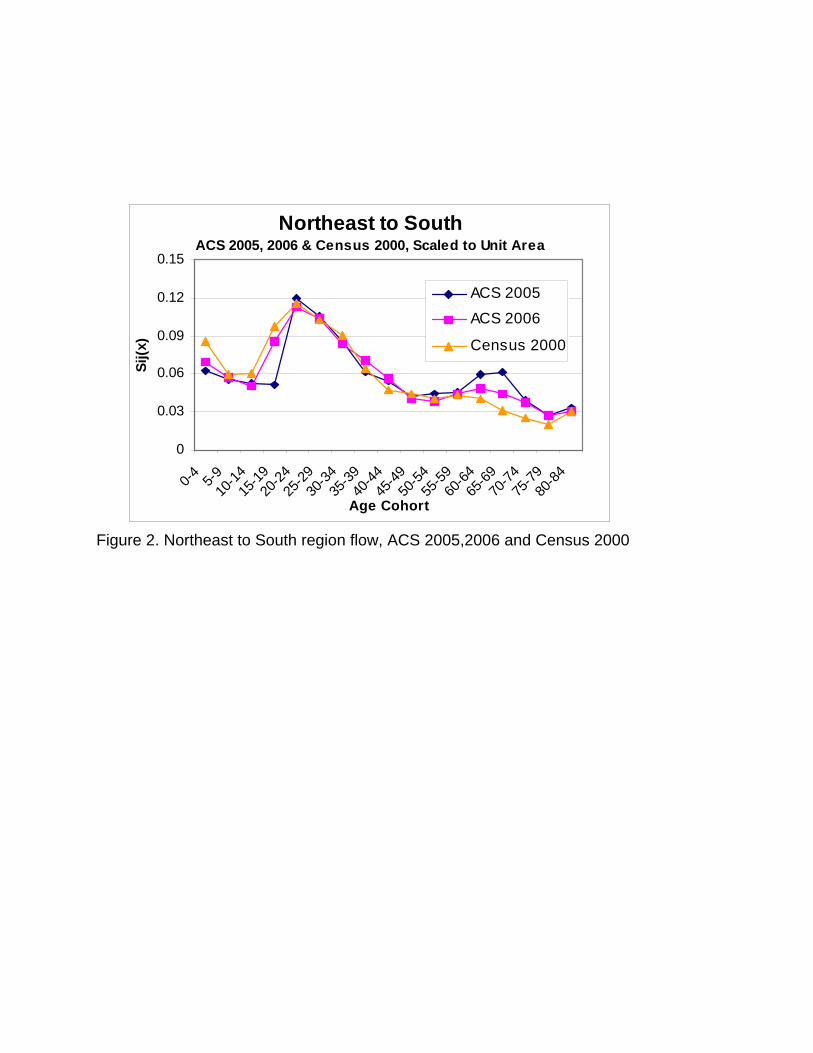
sufficient for us to carry out analyses similar to those of Rogers and Jordan (2004). Figure 2 compares the
Northeast to South regional flow (the regional flow exhibiting the highest age-specific propensities) for
Census 2000, and ACS 2005-2006, scaled to unit area.6 Note that the only major variations are due to the
one-year / five-year problem, that is, the different time periods (ACS vs. Census) over which the migration
question is defined. We expect that the ACS data are actually more accurate, given the finer temporal
resolution realized from a one-year question.
Figure 2 about here
2.2.2 The 4x1 Spatial Scale
By aggregating the out-migration flows from each of the four US Census regions, we can re-examine
the data at the 4x1 spatial scale. Aggregation of the data is useful in that as we increase the number of
“movers” in each analysis, we improve the age-profile of migration. Because the 4x4 data for ACS 2005-
6 To illustrate differences in observed profiles resulting from the 1-year/5-year nature of the ACS/Census data sets.
2006 appear to be adequate for our intended analyses, this exercise is not necessary at the four-region scale.
However, we expect that smaller levels of aggregation (i.e., states as opposed to regions) will be problematic
given the significantly smaller samples sizes, due both to the smaller geographic regions adopted, and to the
reduced sample size of the ACS for those regions. Figure 3 exhibits the four out-migration flows from each
region. Note the normal age-pattern of migration from all regions, as well as the observed retirement peak
from the Northeast region. Lost at this level of aggregation is the destination of those persons contributing to
the observed Northeast retirement peak (largely the South region), demonstrating the disadvantages
associated with larger levels of aggregation.
Figure 3 about here
2.2.3 The 51x1 Spatial Scale
Issues specific to the 51x1 spatial scale include, first and foremost, those related to sample size. The
observed profile of the age-specific migration schedule for out-migration from each state is influenced by the
population of that state. Because the ACS is roughly a 1 in 40 sample, states with smaller populations have
only a very small number of persons surveyed. The impact of the sample size is much larger when we
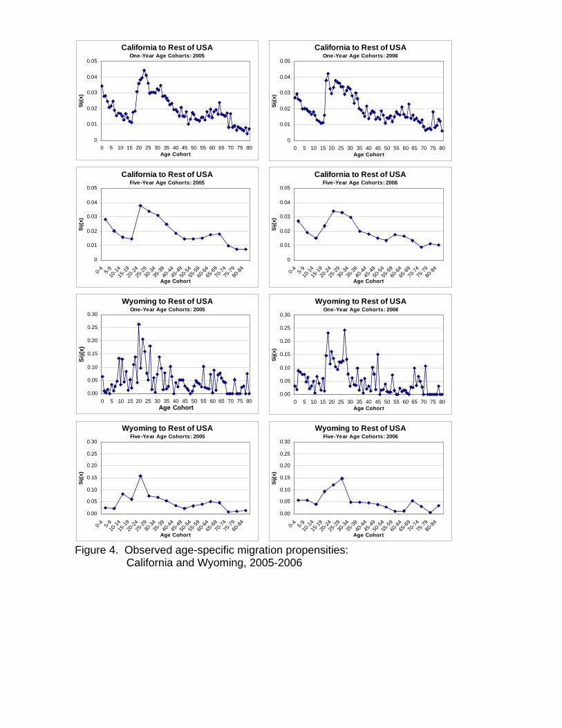
consider each age cohort individually.7 To illustrate this, we will highlight two states in particular:
California and Wyoming. These states represent opposite ends of the population size spectrum, with
California having some 70 times the number of persons found in Wyoming. Consequently, we are likely to
see very different results in these two states, with the California data serving as an example of “good” data,
and the Wyoming data an example of “problematic” or “bad” data.
Figure 4 about here
Figure 4 presents four migration schedules for both California and Wyoming. The first two
schedules describe the migration propensities of one-year age cohorts from the 2005 and the 2006 ACS, and
7 For example, in the case of Wyoming, with a population of around 500,000, the sample would be around 12,500 persons. If we consider five-year age cohorts up to age 80, or 17 separate age groups, the average sample size would be 735, but would be much smaller in several age groups (particularly the older ones).

the second two illustrate the corresponding propensities for five-year age cohorts. Note that for California
both schedules bear resemblance to the standard model migration schedule age profile. The Wyoming data,
however, do not. The only discernible resemblance to the model migration schedule evident in the one-year
age cohort data for Wyoming is the labor peak occurring just after age 20. The rest of the data points appear
almost random. Moving to five-year age cohorts helps slightly, but it reveals no similarity between the
model schedule and observed data for the pre-labor peak cohorts, a result that is quite likely to be inaccurate
and a consequence of a small sample size.
Depending on the user’s intentions, the California data, in this form, might require little or no repair,
and probably are fairly accurate. The Wyoming data clearly require some “repair” if any meaningful
research is to be conducted using them. In both cases, the simplest transformation is from one-year to five-
year age cohorts (already completed here). Additionally this transformation gives the ACS data the same age
groups (but still a different time interval) as the census data.8 Moreover, this transformation removes some
of the “noise” in the model profile associated with minor one-year fluctuations. However, the transformation
alone will not solve problems associated with small sample size, nor will it entirely remove the effect of
outliers in the data. Further transformations are necessary if the observed data, particular in cases like
Wyoming, are to represent reality accurately.
2.3 The Linear Relationship and Infant Migration Method
As alluded to earlier in this paper, the motivation for this work is largely a desire to continue research
into indirect methods of estimating migration propensities. In particular, the authors seek to continue testing
the infant migration method, which we will now briefly describe.
Figure 5 about here
Rogers and Jordan (2004) demonstrated the relationship between a region’s infant migration
propensities and the corresponding migration propensities of all other age cohorts. Using 2005 ACS data 8 The migration data should be in five-year age cohorts if it is to be used with the infant migration methodology discussed later. Five-year data have the advantage of being smoother and more consistent, leading to better results when it comes to estimation.

from the four-region migration model, Figure 5 plots the infant migration propensity (Sij(-1)) and the
corresponding migration propensity for all other age cohorts (Sij(+)) as well as the best fitting line, obtained
from a bivariate regression in which Sij(+) is dependent upon Sij(-1). An R2 value of 0.84 for the 2005 ACS
data (Figure 5) indicates a strong relationship between the variables, signifying that Sij(-1) is a potentially
powerful predictor of migration propensity among other age cohorts.
The use of the infant migration propensity as a starting point is advantageous in that, in the absence
of reported migration data, its level can be approximated by the birthplace-specific population count of
children who are 0-4 years old9 and residing in region j at the time of the census, and who were born in
region i, within the past five years, and therefore who must have migrated during the immediately preceding
5-year interval. Since they were, on average, born some 2-1/2 years ago, it is unlikely that they moved more
than once. Hence, back-casting their numbers to their region of birth, as well as all those of other infants
born in the same region, one is then able to divide each i to j migration number by the total (“surviving-to-
census”) births in i, to obtain an estimate of each of the infant “conditional-on-survival” migration
probabilities, Sij(-5).10 Observed regularities in patterns of age-specific migration probabilities suggest that
information on the probabilities of infant migration also can be linked to the corresponding probabilities in
each of the subsequent age groups by means of a regression equation (Rogers and Jordan, 2004). We,
therefore, can consider a linear regression that links each age-specific Sij(x) with Sij(-5):
termerrorSbaxS ijij +−+= )5()( (2)
Using this simple linear regression equation, the estimated migration propensities for each of the subsequent
five-year age cohorts can be determined.
3. SMOOTHING THE DATA
9 We use five-year age cohorts with Census data. When using the ACS and the one-year migration question, we use children aged 0-1, or Sij(-1). The variability in this measure (as opposed to the more consistent Sij(-5) value) may complicate the use of the infant migration model. Further research is necessary to assess the significance of this difference. 10 For a formal definition of Sij(-5) see Rogers (1995) p. 98.

In some instances, particularly those where the sample size is small, regional migration flows have
exhibited irregularities in their age-specific patterns of migration. In such cases, it is useful to use an age-
specific model migration schedule to smooth out these irregularities. This not only eliminates the
irregularities, but also enforces a profile that is consistent with commonly observed data.
This study employ established characteristics of the ‘normal’ migration schedule to smooth observed
ACS migration data. We apply a methodology previously used to repair data irregularities in studies of the
indirect estimation of migration using Mexican and Indonesian census data (Rogers et. al. 2007) and United
States Census data (Rogers and Jones 2007). This method uses the cubic spline and the seven- or eleven-
parameter model migration schedules11 to smooth data irregularities and impose the proto-typical age-profile
of migration. The resulting model schedule fits (called fitted data) are then used in place of the one-year
observed data. In cases where this data smoothing procedure alone is inadequate, we take further steps to
repair the data. These procedures are discussed in Section Four.
3.1 The Cubic Spline and the Model Schedule Fit
We begin with observed ACS migration data using five-year age cohorts at the 51x1 spatial scale
(See Figure 6.1). Using a program written in MATLAB12 we apply a cubic spline constructed of third-order
polynomials that pass through a set of pre-defined control points, namely, the five-year age group cohort
propensities. A new set of one-year migration propensities is thereby obtained by interpolations using the
cubic spline (Figure 6.2). One-year data are preferred to five- year data because they provide significantly
more data points to which the model schedule can be fitted; however, the original observed one-year data are
inadequate in that they are inaccurate and contain potentially significant outliers. The resulting cubic splined
data set is then fitted by the appropriate model migration schedule (Figure 6.3), again using the MATLAB
based program, producing a final set of one-year age cohort propensities. This data set, whether viewed in
11 The seven-parameter model schedule is used for state out-migration flows where no retirement peak is evident, and the eleven-parameter model in cases where a significant retirement peak is observed. 12 In this study we use a program written in MATLAB by Avleen Bijral and Jani Little.

one- or five-year age cohorts, reflects the appropriate model migration age profile, while preserving observed
levels of migration.
Figure 6 about here
Figure 6 illustrates the process using the observed 2005 ACS data for out-migration from California,
a state that exhibits a retirement peak, and therefore requires an eleven-parameter model schedule fit.
3.2 Results for ACS 2005-2006: 51x1
Assessing the accuracy of our fitted data is somewhat problematic. Because we doubt the accuracy
of many of the observed data, particularly in the case of states with small populations, a simple comparison
of observed and fitted data may not tell us much. But, in the case of larger states, where the observed data
reflect the normal age-profile of migration, such a comparison is useful in assessing the technique. We use
the R² value between the splined observed data and the model-schedule fitted data to judge the accuracy of
the latter. Table 1 presents the 50 states and the District of Columbia in rank order by population size and the
observed R² value that is associated with the model schedule fit. We note that, in general, states near the top
of the list exhibit higher R² values, which we expect given the larger sample size associated with those states.
Table 1 about here
Figure 7 about here
Figure 7 presents visually the decline in R² associated with the smaller state populations. Note the marked
change in the moving average13 of R² after the 26th state in rank order (Kentucky). This point corresponds
with a state population of 4 million, suggesting that for states with a population under 4 million, the ACS
sample size becomes too small to guarantee a “normal” age profile of out-migration. As a result, we surmise
that fitted data for states with less than 4 million people cannot be considered accurate, since the fit itself
13 A five state moving average, moving through states in descending order of population size.

reflects serious inaccuracies in the observed data. Therefore, further action is necessary to adequately repair
data for these smaller state populations.
Figure 8 about here
Figure 8 presents the fitted curves for California and Wyoming (2005). Note the similarity between
the observed and fitted data for California, the state with the largest population and ACS sample size. The
fitted data accurately represent age-specific migration propensities, and in this smoothed form require no
further modification to be used by demographers, planners, or researchers. Conversely, the fitted data for
Wyoming are not at all similar to the observed data, with the exception of the expected higher propensities in
the early adult years. The observed data exhibit little resemblance to the model schedule, most likely
because of a small sample size. The fitted data14 reflect the inconsistencies of the observed data, exhibiting
few of the features of the model migration schedule. In particular, note the location of the pre-labor low-
point, occurring at age 0. From past research we know that younger children migrate more than older
children, because young adults migrate more than older adults (as even this flawed data set indicates).
Therefore, we reject the fitted data set for Wyoming and move on to the repair process for it and other small
states.
4. REPAIRING THE DATA
In this section we discuss a method that we have used to repair the ACS migration data, so that the
flow probabilities, for which a cubic spline fix followed by a model schedule fit do not produce meaningful
and usable results, can be improved. Such a methodology becomes most necessary in cases such as that of
Wyoming, where the fitted results do not exhibit the characteristics of the model migration schedule and
appear to be unrealistic representations of reality. The method presented below illustrates our ongoing
attempt to determine the best manner with which to “correct” the ACS migration data and continue our
research on the indirect estimation of migration.
14 MATLAB fits the model schedule to observed data using a least sum-of-squares principle.

4.1 Defining Families of Out-Migration Flows
The results set out in Section Four suggest that the fitted data for states with populations of over 4
million are fairly good representations of reality. However, for states with less than 4 million people, it is
more difficult to justify such an assertion; for them we propose a procedure for repairing their migration
schedules, using some of the characteristics of the more realistic schedules for states with populations of over
4 million.
Beyond population size, specific interstate migration flows often exhibit characteristics that allow us
to identify different groups of flows. Each “family” of flows exhibits the same defining characteristics, such
as the presence or absence of a retirement peak. Another characteristic is the relative location of the labor
force peak on the horizontal axis, with some peaks occurring at younger (or older) ages than others. The
ratio of the labor force peak value (as reflected by 2a ) to the initial infant migration value (as reflected by 1a )
defines the flow to be either a labor dominant or child dominant flow (Rogers and Castro, 1981). In this
paper we divide the 51 state out-migration flows into three families. First, those flows exhibiting a
retirement peak are separated from those that do not. Second, we define those flows not exhibiting a
retirement peak as being either labor or child dominant. Figure 9 illustrates these distinctions, which we use
to create families of migration flows.
Figure 9 about here
If we take our initial distinction, population size, into account, we are left with a six-division
classification (Table 2) as each of the three families is divided into states with populations above or below 4
million.
Table 2 about here
4.2 Repairing Out-Migration Flows for Small States
After defining families of migration flows, we consider the members of each family that have
populations over 4 million. In these cases, the fitted data are considered to be accurate and acceptable. At

this point, it is important to note that the family distinctions are based upon differences in the profile of the
age-specific model migration schedule, as opposed to the level associated with each flow. We expect
members of the same family to exhibit similar age profiles, but varying levels of migration. Therefore, it is
reasonable to conjecture that those states with fewer than 4 million persons should have out-migration flows
with profiles similar to the profiles of those states with more than 4 million persons and which happen to be
in the same family (e.g., Delaware should have an age profile that is similar to that of Pennsylvania). Thus,
to repair the flows of small states, we take the averages of the observed profile parameters from the large
states (by family), and then impose these parameters onto the flows from the small states (by family). For
each small state flow, we use the observed level parameters and the imposed age profile parameters to create
a more realistic migration schedule, Finally, we impose the observed gross-migraproduction rate15 (GMR) by
rescaling the fitted data, thus ensuring that no changes arise in the state level of out-migration.16
4.3 Results for Small States: ACS 2005-2006, 51x1
As is the case with our smoothing procedure, an assessment of the results produced by the process of
repair is somewhat problematic. Because there is not an “adequate” migration data set from the ACS for the
small states against which to compare our results, we must come up with alternative assessment methods.
We suggest two visual procedures: checking the repaired model schedules against the observed data for
major variations in level, and checking the repaired model schedules against the adopted standard model
schedule to look for major variations in age profile. The former is controlled for in the repair process,
ensuring that overall migration (non-age specific) levels do not deviate from the observed levels. However,
we do not control age-specific levels except at age 0 and that of the labor peak.17 Therefore, we check the
15 The gross migraproduction rate (GMR) is the sum of the migration rates or probabilities for each single year age cohort across a population at a given time (i.e., the total area under the migration schedule curve.). This variable measures the total level of migration out of a region, and can be used to examine the levels of both total regional out-migration and destination-specific regional out-migration (Rogers, 1995). It is analogous in concept to the widely used gross reproduction rate (GRR), which is used to describe the level of fertility rates or probabilities. 16 This maintains a 0 net migration rate nationwide. 17 We use a1 and a2 from the fitted data as initial level parameters; these correspond to migration propensity at age 0 and the labor-force peak.

repaired data to look for any major variations from the observed data for each age-cohort. Any perceived
variation must be carefully considered to determine if it is likely due to a problem with the repaired data, or
is an outlier in the observed data that is causing the variation.
The second visual check ensures that the repaired data reflect the established age-profile of migration.
For instance, in many cases fitted data for the small states failed accurately to capture the profile of pre-labor
force peak migration. The repair procedure is designed to address this problem by imposing the profile
parameters obtained from other, more adequate data sets.
Figure 10 about here
The results for the 25 smallest states were generally satisfactory, passing both of the above mentioned
visual checks. However, in the case of the state with the smallest population and sample size, Wyoming, the
results are questionable (Figure 10). The age-profile itself is much improved, and for both 2005 and 2006
the pre-labor force peak shape is normal. However, the 2005 12 aa ratio reflects labor dominance (the
designated family for Wyoming), while the 2006 12 aa ratio reflects the opposite: child dominance.
Additionally, significant variations in level exist between the observed and the repaired data for most age-
cohorts. Because the observed pre-labor force curve data do not follow the model schedule, we expect
considerable variation at specific ages in this portion of the curve. In the repaired 2005 data, the overall
levels of pre-labor force peak migration (observed and repaired) appear the same, the repaired data simply
exhibit the appropriate profile. But, the 2006 repaired data indicate a much higher level of pre-labor force
peak migration. Therefore, despite the improved profiles, we cannot assume this portion of the repaired
curve to be a more accurate representation of reality.
The 2005 repaired data become problematic when considering the labor / adult portion of the curve.
From roughly ages 23 to 38 (including the labor peak) we note significantly higher propensities in the
repaired data. From age 38 onward we note lower propensities in the repaired data. The 2006 repaired data
appear better, reflecting the observed labor peak level, albeit at a much earlier age. The latter portion of the
repaired curve appears to be a better approximation of observed levels than did the latter part of the 2005

repaired curve. But, because the observed data for Wyoming are based on such a small sample, and exhibit
such abnormal tendencies, we have little basis to either accept or reject any repaired data set on the basis of a
visual comparison.
Figure 11 about here
Wyoming, however, is an exceptional case. For the most part, the rest of the results are quite
reasonable. Figure 11 presents the observed and repaired data for another small state: Rhode Island. Note
that many of the inconsistencies in the observed Rhode Island data are similar to those that we noted in the
Wyoming data. Also note that the similarly corrected pre-labor force peak profile in the repaired data again
appear to preserve expected pre-labor force peak migration levels. But the repaired Rhode Island data
deviate from those of Wyoming in that no major variations in age-specific levels exist in the labor / adult
portion of the curve, and the repaired data accurately maintain observed levels while correcting the age-
profile inconsistencies. In this case we are more likely to accept the repaired data as reflecting an accurate
representation of reality.
Again, because of the nature of the observed data, it is difficult to assert that the repaired data are
more accurate than the original ones. To further improve our ability to make such assertions, we recommend
checking the repaired data against the corresponding observed data from Census 2000, a data set we consider
accurate. However, one must be cautious with such a comparison because of the variations in the nature of
Census / ACS data discussed earlier (e.g., the 1-year/5-year problem.
5. CONCLUSIONS
5.1 Comparisons to Census 2000: The 1-year / 5-year Problem
To further assess the usefulness of the procedure described in Section 4 we can compare the resulting
migration schedules to those derived from the 2000 census.18 Figure 12 provides a comparison of the ACS
and Census data for California and Wyoming (one-year age-cohorts). The first two graphs preserve level,
18 The 2000 Census data also have had the cubic spline and model schedule fit applied prior to the comparison.

while the second two scale the curves to unit area, allowing us to better compare pure profiles. Several
obvious differences exist. First, there is the expected difference in levels resulting from the longer exposure
time in the Census migration question.19 Naturally we expect persons to have a higher migration propensity
over a five-, as opposed to just one-year period. But as Rogers et al. (2003) point out, the relationship
between the 1-year and 5-year data is not a simple five-to-one ratio. The 5-year question is likely to miss
many return and onward migrations; thus, the true ratio is probably somewhere between three-to-one and
four-to-one, depending on the individual flow in question. Establishing and using this crude ratio for each of
our individual flows may prove to be a useful extension in future research.
Figure 12 about here
Second, we notice that in both the normal and standardized graphs, the labor peak appears to occur at
a later age in the ACS data, for both California and Wyoming. This is, once again, likely due to data
differences arising as a result of 1-year / 5-year questions. Furthermore, the difference in the location of the
adolescent low-point, and the gap between the ACS and Census data in the positively sloped portion of the
labor curve are likely a result of the same problem.
Finally, we notice that, with the exception of issues related to the 1-year / 5-year problem, the
California ACS data appear very similar to the Census data, further bolstering our assertion that the fitted
ACS data for California are reliable. However, significant differences beyond those related to 1-year / 5-
year issues exist in the Wyoming ACS data. There is a significant difference in the height of the labor peak
in the standardized curve, which raises questions about the nature of out-migration from Wyoming: which
curve is correct? Given the significantly larger sample size associated with the Census, we believe that the
Census curve is likely the more accurate one of the two, conceding of course that the Census data provide
different indication concerning the exact ages of the low point and the labor peak, as well as the pattern of
migration between the two.
19 A five-year question, as opposed to the one-year question in the ACS.

There are several papers that acknowledge the so-called 1-year / 5-year problem, for example,
Rogers, et al. (2003), and Franklin and Plane (2006). There are many problems related to the comparison of
migration data derived from 1-year and 5-year questions. This paper is concerned with those issues that
directly affect our ability to use the infant migration model with ACS data such that we can compare results
from the Census and ACS. Therefore, there are two specific issues we will discuss here (illustrated in Figure
13).
Figure 13 about here
The first issue relates to the location of the labor peak. The ACS peak is consistently located between
4 and 7 years to the right of the Census peak. This can be at least partially explained by considering the
construction of the curves, and the nature of 1-year / 5-year relationships. When we visually examine the
age-specific model schedule, we must ask what year(s) the schedule is illustrating. The answer is directly
related to the type of migration question asked. In the case of the Census, the migration question asks
respondents where they live now, and where they lived five years ago. When we display results (using the
2000 Census data for example) in the form of the age-profile, we are displaying the prospective propensity of
each age-cohort to migrate as if it were 1995. Thus the first age cohort consists of children who were
between ages 0 and 4 in 1995, but 5 to 9 in 2000. Thus we are, in essence, back-casting five years. This is
done because in our infant migration model, the propensities of children born between 1995 and 2000, is the
Sij(-5) value used as our independent variable. Furthermore, because this “infant” population is only
exposed to the risk of migration for, on average, half the time (2 ½ years), their propensity will not have the
same meaning as those from the other age-cohorts.
In the case of ACS data and a 1-year migration question, we are only back-casting one year, and thus
are using Sij(-1) as the independent variable. Again, the propensity for this group will have a different
meaning than all the others, because the population in question will only have, on average, 6 months of
exposure. The four year difference in back-casting at least partially explains the observed lag in the position

of the labor peak. However, in some cases the lag is either shorter or longer than four years, indicating that
some other factor is also contributing to the difference.
The second issue, apparent in the scaled-to-unit-area (Figure 11) comparison, is the decidedly steeper
slope in the pre-labor peak portion of the labor curve in the ACS data. Furthermore, we notice that the low
point occurs later in the ACS data, and is somewhat lower in the Census data. These two factors lead to a
noticeable “gap” between the pre-labor peak portions of the labor peak curves. The lag in the position of the
low point is explained, at least partially, by the back-casting issue discussed above. However, it is also quite
likely that we are looking at one consequence of the superior resolution provided by the ACS. The 5-year
question used in the census will inevitably “smooth” out the data, making the curve easier to interpret and
work with, but costing researchers some information as well. Although 1-year fluctuations can be
troublesome and misleading, one advantage of using a 1-year question is that it allows one to better examine
migration behavior during those crucial time periods throughout the life course, at which propensities are the
most likely to change dramatically, or to reach peaks and valleys.
The time between the adolescent low point and the labor peak is an example. In developed countries
such as the United States, the low point typically occurs during a teenager’s final year of high school. The
following year, we notice a jump in migration propensity, as these young adults leave their parental homes,
for example, to attend college, begin a working career, or join the military. The increase in propensity
continues for several years, peaking sometime in the early to mid-20’s, and then gradually declines
throughout the adult years. The use of a one-year migration question allows the researcher to observe this
process much more closely, assuming of course that the sample size for the flow in question is adequate. In
the case of California (Figure 10), for example, it is quite possible that it is the ACS data that more
accurately depict the low-point and labor-curve peak propensities. But, this assertion cannot be confirmed.
If the ACS data are correct, we need to reconsider the use of the Census data as the benchmarks, in the case
of states like California.
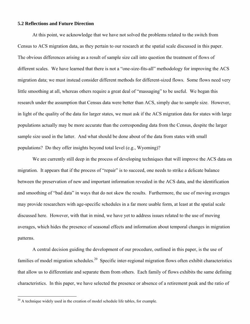
5.2 Reflections and Future Direction
At this point, we acknowledge that we have not solved the problems related to the switch from
Census to ACS migration data, as they pertain to our research at the spatial scale discussed in this paper.
The obvious differences arising as a result of sample size call into question the treatment of flows of
different scales. We have learned that there is not a “one-size-fits-all” methodology for improving the ACS
migration data; we must instead consider different methods for different-sized flows. Some flows need very
little smoothing at all, whereas others require a great deal of “massaging” to be useful. We began this
research under the assumption that Census data were better than ACS, simply due to sample size. However,
in light of the quality of the data for larger states, we must ask if the ACS migration data for states with large
populations actually may be more accurate than the corresponding data from the Census, despite the larger
sample size used in the latter. And what should be done about of the data from states with small
populations? Do they offer insights beyond total level (e.g., Wyoming)?
We are currently still deep in the process of developing techniques that will improve the ACS data on
migration. It appears that if the process of “repair” is to succeed, one needs to strike a delicate balance
between the preservation of new and important information revealed in the ACS data, and the identification
and smoothing of “bad data” in ways that do not skew the results. Furthermore, the use of moving averages
may provide researchers with age-specific schedules in a far more usable form, at least at the spatial scale
discussed here. However, with that in mind, we have yet to address issues related to the use of moving
averages, which hides the presence of seasonal effects and information about temporal changes in migration
patterns.
A central decision guiding the development of our procedure, outlined in this paper, is the use of
families of model migration schedules.20 Specific inter-regional migration flows often exhibit characteristics
that allow us to differentiate and separate them from others. Each family of flows exhibits the same defining
characteristics. In this paper, we have selected the presence or absence of a retirement peak and the ratio of
20 A technique widely used in the creation of model schedule life tables, for example.

the labor force peak value to the initial infant migration value, to define the flows as being either labor or
child dominant (Rogers and Castro, 1981). In doing this, we divide the state out-migration flows into three
families.
This technique also has allowed us to address problems related to scale. After dividing states in each
family into those with greater than 4 million persons, and those with less, we imposed the average profile
parameters, derived from those states in the family with a population above 4 million, onto the states with
less than 4 million, while preserving the observed level parameters for these states. We believe that the
schedule’s age profile is more adversely affected by small sample size than is its level. Age-cohort sample
sizes, in the case of 5-year age-groups, are some 15-20 times smaller than the total sample size, from which
overall level is ultimately determined. Thus, by preserving overall levels but imposing age profiles, we
conserve the more accurate characteristics of the data set, and alter those more likely to be incorrect.
However, if we were to expand the scale of the study to focus on, say, a 51x51 matrix of flows, we likely
would be unable to adequately deal with sample size issues present in the data that purport to describe, for
example, the lightly traveled migration routes, from Wyoming to Rhode Island, say.
It is clear that the switch to ACS migration data will be difficult for many involved in migration
research. Moreover, it is also apparent that the use of ACS data offers exciting possibilities, including but
not limited to a dramatic increase in the information one may derive from examination of the 1-year data.
The process of switching to ACS migration data will vary from one researcher to another, depending upon
the intended use of the data. We hope that our experience will help others involved in the process to better
understand the pitfalls and possibilities associated with the development of the needed graduation
techniques.
REFERENCES
Alexander, C.H. (1997), The American Community Survey Design Issues and Initial Test Results. Census Bureau Publication, ACS Operations Plan, U.S. Bureau of the Census, Washington D.C.
Alexander, C.H. (2001), Integrating the American Community Survey and the Intercensal
Demographic Estimates Program. Census Bureau Publication, ACS Operations Plan, U.S. Bureau of the Census, Washington D.C.
Franklin, R. and Plane, D. (2006), Pandora’s Box: The Potential and Peril of Migration Data from the
American Community Survey. International Regional Science Review 29(3): 231-246 Mather, M., Rivers, K.L., Jacobsen, L.A. (2005), The American Community Survey. Population
Bulletin 60, no. 3, Washington DC: Population Reference Bureau. Rogers, A., (1995), Multiregional Demography: Principles, Methods, and Extensions. John Wiley,
London.
Rogers, A. and Castro, L.J. (1981), Model Migration Schedules. Research Report. Laxenburg, Austria: International Institute for Applied Systems Analysis.
Rogers, A. and Jones, B. (2007), Inferring Directional Migration Propensities from the Migration
Propensities of Infants: the United States. Population Program, Institute of Behavioral Science, University of Colorado, Boulder, forthcoming in Mathematical Population Studies.
Rogers, A., Jones, B., Partida, V., and Muhidin, S. (2007), Inferring Migration Flows from the
Migration Propensities of Infants: Mexico and Indonesia. The Annals of Regional Science 41:443-465.
Rogers, A. and Jordan, L. (2004), Estimating Migration Flows from Birth-Specific Population Stocks
of Infants. Geographical Analysis 36(1): 38-53.
Rogers, A., Raymer, J., and Newbold, K.B. (2003), Reconciling and Transferring Migration Data Collected Over Time Intervals of Differing Widths. The Annals of Regional Science 37: 581-601.

Table 1. Population, sample size, and R² (splined & fitted data), 2005-2006
State 2005 2006 2005 2006 2005 2006California 35,340,566 36,457,549 345,723 334,885 0.98 0.99Texas 22,250,152 23,507,783 226,724 217,617 0.98 0.99New York 18,679,211 19,306,183 187,143 181,406 0.98 0.98Florida 17,363,653 18,089,889 185,309 177,000 0.96 0.96Illinois 12,441,864 12,831,970 126,613 123,074 0.98 0.99Pennsylvania 11,948,862 12,440,621 124,455 121,424 0.98 0.99Ohio 11,146,050 11,478,006 117,593 114,707 0.99 0.98Michigan 9,857,477 10,095,643 101,355 99,784 0.95 0.97Georgia 8,811,648 9,363,941 91,896 87,534 0.97 0.99New Jersey 8,524,868 8,724,560 86,190 83,991 0.98 0.95North Carolina 8,397,785 8,856,505 89,124 85,611 0.99 0.99Virginia 7,320,848 7,642,884 76,649 73,509 0.98 0.98Massachusetts 6,200,944 6,437,193 64,673 62,695 0.98 0.99Washington 6,157,786 6,395,798 63,524 61,520 0.97 0.98Indiana 6,081,212 6,313,520 65,054 63,278 0.96 0.97Tennessee 5,816,359 6,038,803 61,139 59,376 0.98 0.95Arizona 5,806,266 6,166,318 60,195 58,315 0.96 0.88Missouri 5,632,603 5,842,713 59,696 57,884 0.99 0.99Maryland 5,453,441 5,615,727 55,683 54,290 0.97 0.93Wisconsin 5,401,740 5,556,506 57,987 56,368 0.98 0.98Minnesota 4,969,152 5,167,101 52,219 50,857 0.98 0.99Colorado 4,540,639 4,753,377 48,020 46,094 0.97 0.96Alabama 4,448,075 4,599,030 47,018 45,534 0.98 0.94Louisiana 4,387,181 4,287,768 40,901 43,956 1.00 0.96South Carolina 4,127,391 4,321,249 43,829 41,956 0.95 0.97Kentucky 4,065,635 4,206,074 42,429 41,498 0.97 0.93Oregon 3,560,922 3,700,758 36,499 35,485 0.93 0.96Oklahoma 3,429,974 3,579,212 35,781 34,683 0.95 0.97Connecticut 3,365,768 3,504,809 35,070 33,867 0.94 0.99Iowa 2,848,266 2,982,085 30,883 29,629 0.99 0.93Mississippi 2,830,388 2,910,540 28,945 28,354 0.97 0.93Arkansas 2,694,665 2,810,872 28,343 27,399 0.94 0.95Kansas 2,669,699 2,764,075 28,168 27,462 0.95 0.97Utah 2,452,149 2,550,063 25,746 24,749 0.96 0.97Nevada 2,376,017 2,495,529 24,858 23,538 0.71 0.89New Mexico 1,886,789 1,954,599 18,637 18,272 0.94 0.83West Virginia 1,781,817 1,818,470 18,446 17,771 0.97 0.88Nebraska 1,706,343 1,768,331 18,063 17,442 0.90 0.94Idaho 1,408,650 1,466,465 14,931 14,353 0.81 0.93Maine 1,282,474 1,321,574 12,649 12,440 0.95 0.94New Hampshire 1,271,897 1,314,895 12,818 12,758 0.95 0.93Hawaii 1,258,528 1,285,498 12,891 12,743 0.93 0.98Rhode Island 1,033,284 1,067,610 10,576 10,184 0.88 0.96Montana 897,367 944,632 9,052 8,715 0.94 0.95Delaware 825,598 853,476 8,115 7,933 0.91 0.90South Dakota 755,152 781,919 8,044 7,667 0.92 0.92Alaska 658,002 670,053 6,327 6,129 0.69 0.85North Dakota 621,063 635,867 6,699 6,505 0.94 0.95Vermont 609,857 623,908 6,183 5,896 0.96 0.98District of Columbia 508,572 581,530 5,577 5,187 0.87 0.95Wyoming 494,170 515,004 5,299 5,056 0.73 0.86
Population Sample Size R²
* The generally smaller sample sizes in 2006 reflect a smaller overall sample, despite population increases in most states.

Table 2. Family classification by population sizeFamily Top 26 Bottom 25
Pop > 4,000,000 Pop < 4,000,000Retirement Peak California
IllinoisMassachusettsNew JerseyNew YorkOhio
Labor Dominant Florida AlaskaMichigan ConnecticutMinnesota DelawarePennsylvania District of ColumbiaSouth Carolina IdahoWisconsin Iowa
NevadaNew MexicoNorth DakotaWyoming
Child Dominant Alabama ArkansasArizona HawaiiColorado KansasGeorgia MaineIndiana MississippiKentucky MontanaLouisiana NebraskaMaryland New HampshireMissouri OklahomaNorth Carolina OregonTennessee Rhode IslandTexas South DakotaVirginia UtahWashington Vermont
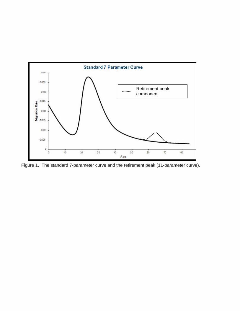
Figure 1. The standard 7-parameter curve and the retirement peak (11-parameter curve).
Retirement peak component
Northeast to SouthACS 2005, 2006 & Census 2000, Scaled to Unit Area
0
0.03
0.06
0.09
0.12
0.15
0-4 5-910
-1415
-1920
-2425
-2930
-3435
-3940
-4445
-4950
-5455
-5960
-6465
-6970
-7475
-7980
-84
Age Cohort
Sij(x
)
ACS 2005
ACS 2006
Census 2000
Figure 2. Northeast to South region flow, ACS 2005,2006 and Census 2000

4x1 Out-Migration Flows
ACS 2006
0
0.01
0.02
0.03
0.04
0-4 5-910
-1415
-1920
-2425
-2930
-3435
-3940
-4445
-4950
-5455
-5960
-6465
-6970
-7475
-7980
-84
Age Cohort
Sij(x
)
NortheastMidwestSouthWest
4x1 Out-Migration FlowsACS 2005
0
0.01
0.02
0.03
0.04
0-4 5-910
-1415
-1920
-2425
-2930
-3435
-3940
-4445
-4950
-5455
-5960
-6465
-6970
-7475
-7980
-84
Age Cohort
Sij(x
)
NortheastMidwestSouthWest
Figure 3. Out-migration from the four US Census Regions, 2005 and 2006
California to Rest of USAOne-Year Age Cohorts: 2006
0
0.01
0.02
0.03
0.04
0.05
0 5 10 15 20 25 30 35 40 45 50 55 60 65 70 75 80Age Cohort
Sij(x
)
California to Rest of USAOne-Year Age Cohorts: 2005
0
0.01
0.02
0.03
0.04
0.05
0 5 10 15 20 25 30 35 40 45 50 55 60 65 70 75 80Age Cohort
Sij(x
)
Figure 4. Observed age-specific migration propensities: California and Wyoming, 2005-2006
California to Rest of USAFive-Year Age Cohorts: 2005
0
0.01
0.02
0.03
0.04
0.05
0-4 5-910
-1415
-1920
-2425
-2930
-3435
-3940
-4445
-4950
-5455
-5960
-6465
-6970
-7475
-7980
-84
Age Cohort
Sij(x
)
California to Rest of USAFive-Year Age Cohorts: 2006
0
0.01
0.02
0.03
0.04
0.05
0-4 5-910
-1415
-1920
-2425
-2930
-3435
-3940
-4445
-4950
-5455
-5960
-6465
-6970
-7475
-7980
-84
Age CohortSi
j(x)
Wyoming to Rest of USAOne-Year Age Cohorts: 2005
0.00
0.05
0.10
0.15
0.20
0.25
0.30
0 5 10 15 20 25 30 35 40 45 50 55 60 65 70 75 80Age Cohort
Sij(x
)
Wyoming to Rest of USAOne-Year Age Cohorts: 2006
0.00
0.05
0.10
0.15
0.20
0.25
0.30
0 5 10 15 20 25 30 35 40 45 50 55 60 65 70 75 80Age Cohort
Sij(x
)
Wyoming to Rest of USAFive-Year Age Cohorts: 2005
0.00
0.05
0.10
0.15
0.20
0.25
0.30
0-4 5-910
-1415
-1920
-2425
-2930
-3435
-3940
-4445
-4950
-5455
-5960
-6465
-6970
-7475
-7980
-84
Age Cohort
Sij(x
)
Wyoming to Rest of USAFive-Year Age Cohorts: 2006
0.00
0.05
0.10
0.15
0.20
0.25
0.30
0-4 5-910
-1415
-1920
-2425
-2930
-3435
-3940
-4445
-4950
-5455
-5960
-6465
-6970
-7475
-7980
-84
Age Cohort
Sij(x
)

The Linear Relationship
0.000.020.040.060.080.100.120.140.160.180.20
0.000 0.003 0.006 0.009 0.012 0.015Sij (-1)
Sij(+
)
ObservedPredicted
Figure 5. Infant migration propensity and propensity for all other ages, 2005 ACS four-region model.
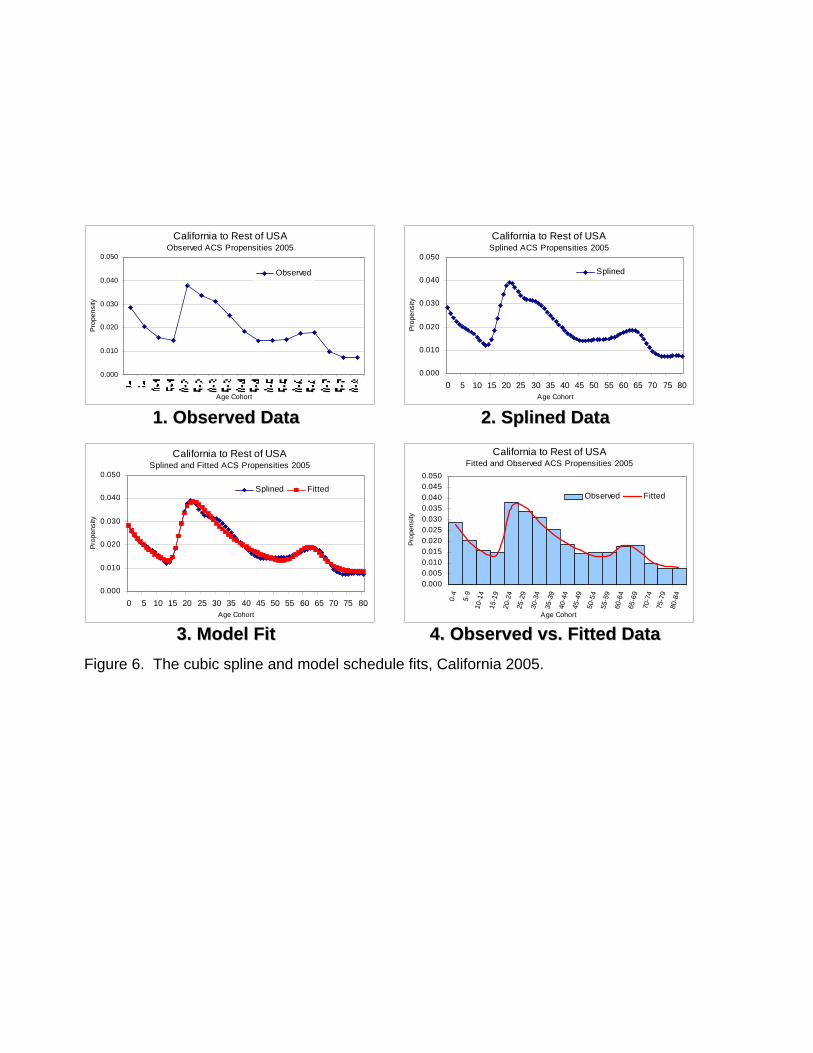
Figure 6. The cubic spline and model schedule fits, California 2005.
33.. MMooddeell FFiitt 44.. OObbsseerrvveedd vvss.. FFiitttteedd DDaattaa
California to Rest of USASplined and Fitted ACS Propensities 2005
0.000
0.010
0.020
0.030
0.040
0.050
0 5 10 15 20 25 30 35 40 45 50 55 60 65 70 75 80Age Cohort
Prop
ensi
ty
Splined Fitted
California to Rest of USAFitted and Observed ACS Propensities 2005
0.0000.0050.0100.0150.0200.0250.0300.0350.0400.0450.050
0-4
5-9
10-1
415
-19
20-2
425
-29
30-3
435
-39
40-4
445
-49
50-5
455
-59
60-6
465
-69
70-7
475
-79
80-8
4
Age Cohort
Prop
ensi
ty
Observed Fitted
11.. OObbsseerrvveedd DDaattaa 22.. SSpplliinneedd DDaattaa
California to Rest of USASplined ACS Propensities 2005
0.000
0.010
0.020
0.030
0.040
0.050
0 5 10 15 20 25 30 35 40 45 50 55 60 65 70 75 80Age Cohort
Prop
ensi
ty
Splined
California to Rest of USAObserved ACS Propensities 2005
0.000
0.010
0.020
0.030
0.040
0.050
Age Cohort
Prop
ensi
ty
Observed
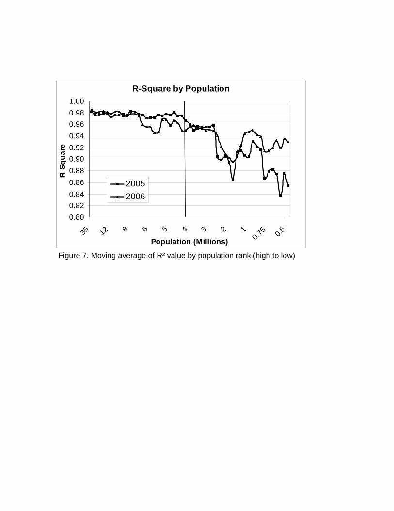
Figure 7. Moving average of R² value by population rank (high to low)
R-Square by Population
0.800.820.840.860.880.900.920.940.960.981.00
35
12 8 6 5 4 3 2 1
0.75 0.5
Population (Millions)
R-S
quar
e
20052006

Figure 8. Results of the model migration schedule fit: California and Wyoming, 2005-2006
California to Rest of USAACS 2005
0.00
0.01
0.02
0.03
0.04
0.05
0 5 10 15 20 25 30 35 40 45 50 55 60 65 70 75 80Age Cohort
Prop
ensi
ty
ObservedFitted
California to Rest of USAACS 2006
0.00
0.01
0.02
0.03
0.04
0.05
0 5 10 15 20 25 30 35 40 45 50 55 60 65 70 75 80Age Cohort
Prop
ensi
ty
ObservedFitted
Wyoming to Rest of USAACS 2005
0.00
0.05
0.10
0.15
0.20
0.25
0.30
0 5 10 15 20 25 30 35 40 45 50 55 60 65 70 75 80Age Cohort
Prop
ensi
ty
ObservedFitted
Wyoming to Rest of USAACS 2005
0.00
0.05
0.10
0.15
0.20
0.25
0.30
0 5 10 15 20 25 30 35 40 45 50 55 60 65 70 75 80Age Cohort
Prop
ensi
ty
ObservedFitted

Figure 9. Characteristics of the model schedule used to designate family membership
2a
1a
3a1α
2α
3α
2λ
3λ
c
1x 2x 3xAge (x)
Mig
ratio
n R
ate
m(x
)
Family Designation
1) Presence or absence of retirement peak(parameters , , and )
2) Ratio of 3λ 3α 3a
12 a/a
Figure 9. Characteristics of the model schedule used to designate family membership
2a
1a
3a1α
2α
3α
2λ
3λ
c
1x 2x 3xAge (x)
Mig
ratio
n R
ate
m(x
)
Family Designation
1) Presence or absence of retirement peak(parameters , , and )
2) Ratio of 3λ 3α 3a
12 a/a2a
1a
3a1α
2α
3α
2λ
3λ
c
1x 2x 3xAge (x)
Mig
ratio
n R
ate
m(x
)
Family Designation
1) Presence or absence of retirement peak(parameters , , and )
2) Ratio of 3λ 3α 3a
12 a/a
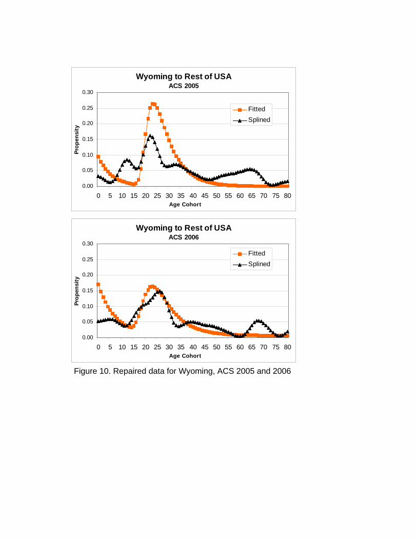
Figure 10. Repaired data for Wyoming, ACS 2005 and 2006
Wyoming to Rest of USAACS 2005
0.00
0.05
0.10
0.15
0.20
0.25
0.30
0 5 10 15 20 25 30 35 40 45 50 55 60 65 70 75 80Age Cohort
Prop
ensi
ty
FittedSplined
Wyoming to Rest of USAACS 2006
0.00
0.05
0.10
0.15
0.20
0.25
0.30
0 5 10 15 20 25 30 35 40 45 50 55 60 65 70 75 80Age Cohort
Prop
ensi
ty
FittedSplined
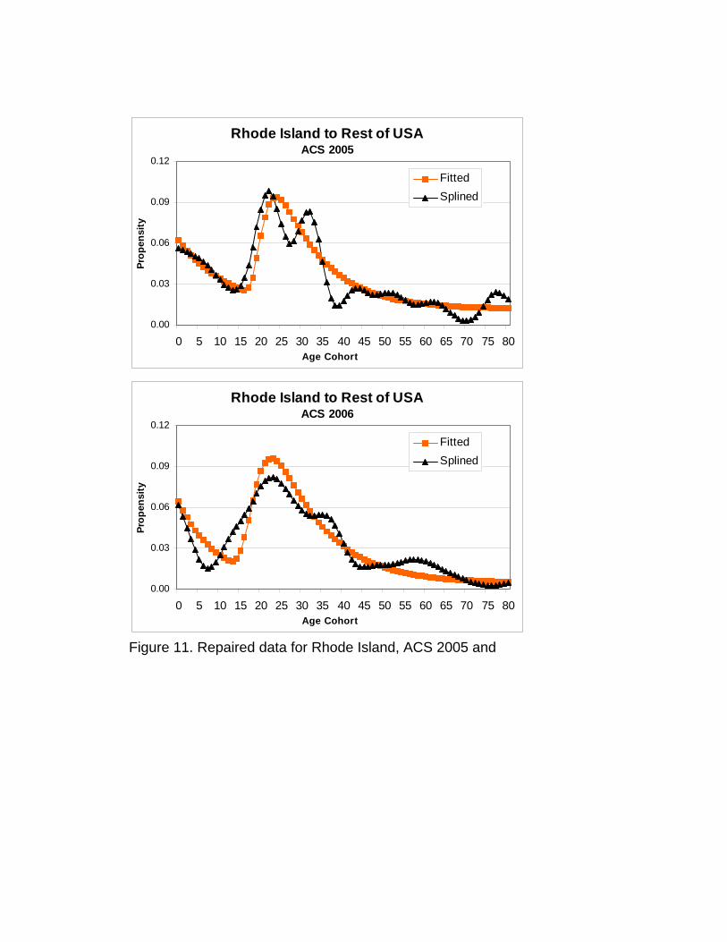
Figure 11. Repaired data for Rhode Island, ACS 2005 and
Rhode Island to Rest of USAACS 2005
0.00
0.03
0.06
0.09
0.12
0 5 10 15 20 25 30 35 40 45 50 55 60 65 70 75 80Age Cohort
Prop
ensi
ty
FittedSplined
Rhode Island to Rest of USAACS 2006
0.00
0.03
0.06
0.09
0.12
0 5 10 15 20 25 30 35 40 45 50 55 60 65 70 75 80Age Cohort
Prop
ensi
ty
FittedSplined

Figure 12. Census 2000 and ACS 2005 age profiles, observed and scaled to unit area, California and Wyoming
California to Rest of USACensus 2000 and ACS 2005
0.00
0.02
0.04
0.06
0.08
0.10
0.12
0.14
0 5 10 15 20 25 30 35 40 45 50 55 60 65 70 75 80
Age Cohort
Prop
ensi
ty
CensusACS
Wyoming to Rest of USACensus 2000 and ACS 2005
0.00
0.05
0.10
0.15
0.20
0.25
0.30
0.35
0.40
0 5 10 15 20 25 30 35 40 45 50 55 60 65 70 75 80
Age Cohort
Prop
ensi
ty
CensusACS
California to Rest of USACensus 2000 and ACS 2005, Scaled to Unit Area
0.00
0.01
0.02
0.03
0 5 10 15 20 25 30 35 40 45 50 55 60 65 70 75 80
Age Cohort
Prop
ensi
ty
CensusACS
Wyoming to Rest of USACensus 2000 and ACS 2005, Scaled to Unit Area
0.00
0.01
0.02
0.03
0 5 10 15 20 25 30 35 40 45 50 55 60 65 70 75 80
Age Cohort
Prop
ensi
ty
CensusACS

Figure 13. The 1-year / 5-year
California to Rest of USACensus 2000 and ACS 2005
0.00
0.02
0.04
0.06
0.08
0.10
0.12
0.14
0 5 10 15 20 25 30 35 40 45 50
Age Cohort
Prop
ensi
ty
CensusACS
California to Rest of USACensus 2000 and ACS 2005, Scaled to Unit Area
0.00
0.01
0.02
0.03
0 5 10 15 20 25 30 35 40 45 50
Age Cohort
Prop
ensi
ty
CensusACS


