Download - Repositioning Dynamics and Pricing Strategy

Repositioning Dynamics and Pricing Strategy�
Paul B. EllicksonUniversity of Rochester
Sanjog MisraUniversity of Rochester
Harikesh S. NairStanford University
January, 2011y
Abstract
We measure the revenue and cost implications to supermarkets of changing theirprice positioning strategy in oligopolistic downstream retail markets. Our estimateshave implications for long-run market structure in the supermarket industry, and formeasuring the sources of price rigidity in the economy. We exploit a unique datasetcontaining the price-format decisions of all supermarkets in the U.S. The data containthe format-change decisions of supermarkets in response to a large shock to their localmarket positions: the entry of Wal-Mart. We exploit the responses of retailers to Wal-Mart entry to infer the cost of changing pricing-formats using a �revealed-preference�argument similar to the spirit of Bresnahan and Reiss (1991). The interaction betweenretailers and Wal-Mart in each market is modeled as a dynamic game. We �nd evidencethat suggests the entry patterns of WalMart had a signi�cant impact on the costs andincidence of switching pricing strategy. Our results add to the marketing literature onthe organization of retail markets, and to a new literature that discusses implications ofmarketing pricing decisions for macroeconomic studies of price rigidity. More generally,our approach which incorporates long-run dynamic consequences, strategic interaction,and sunk investment costs, outlines how the paradigm of dynamic games may be usedto model empirically �rms�positioning decisions in Marketing.Keywords: Positioning, dynamic games, EDLP, PROMO, retailing, pricing, price
rigidity, Wal-Mart.
�Contact Email: [email protected]; [email protected];[email protected].
yThe usual disclaimer applies.
1
It is not necessary to change. Survival is not mandatory.
�W. Edwards Deming
1 Introduction
E¤ective marketing strategy in a dynamic environment requires the ability to foresee the
need for change and a willingness to change direction. In marketing, large changes to some
or all of a �rm�s marketing apparatus are referred to as �repositioning.�
Firms may reposition themselves along a variety of dimensions. Perhaps the most com-
mon (and visible) forms of repositioning are brand and product related. Recent examples
include Domino Pizza�s attempt to switch their reputation from fast delivery to high quality
and the repositioning of UPS from shipping to full o¢ ce solutions (�What can brown do
for you?�). Other examples include adjustments to product lines, such as Hyundai�s recent
move into the luxury auto segment in the U.S. or Kodak�s long-delayed transition to digital
imaging. While product based decisions are clearly the most common form of repositioning,
they are far from the only examples. Apple�s recent inclusion of third party retailers can be
thought of repositioning their distribution strategy, while Proctor and Gamble�s adoption of
�Value-Based Pricing�in 1992 (by reducing trade-promotions) was a repositioning of their
overall pricing strategy (Ailawadi, Lehmann, and Neslin (2001)).
A key aspect of repositioning decisions is that they are inherently dynamic. Sunk in-
vestments in positioning and reputation are often only partially reversible, and have sig-
ni�cant long-term consequences for competitive market structure and future pro�tability.
Forward-looking �rms must consider not only how consumers will react to their decisions,
but whether their rivals will respond in kind. They need also take into account how today�s
decisions impact tomorrow�s options. For example, a promise to o¤er every day low prices
has commitment value, but limits a �rm�s ability to respond to macroeconomic �uctuations.
Taken together, these facets of the decision environment suggest that positioning decisions
in Marketing should be viewed as dynamic games. Furthermore, by framing decisions in
this way, we are able to construct a framework that allows us to structurally estimate the
bene�ts and costs of repositioning.
In this paper we examine the repositioning of supermarket �rms� pricing strategies.
The organization of retail supermarkets for CPG goods in the US is broadly split between
EDLP (Every Day Low Price) and PROMO (or promotional) price positioning strategies.1
1PROMO is also referred to as �HiLo.�
2

EDLP stores charge a low regular price per product with little temporal price variation,
while PROMO stores are characterized by higher regular prices, punctuated by frequent
price promotions or �sales.� The propensity of stores to choose EDLP or PROMO price
positioning is motivated by both demand- and cost-side considerations. On the demand
side, choosing PROMO over EDLP o¤ers an opportunity for supermarkets to intertempo-
rally price discriminate, by using price cycles to sell di¤erentially to consumers of varying
price information, loyalty, stockpiling costs or valuations (Varian (1980); Salop and Stiglitz
(1982); Sobel (1984); Lal and Rao (1997); Pesendorfer (2002); Bell and Hilber (2006)).
Further, the frequent price variation under PROMO creates an option value to consumers
to visiting the store more frequently by reducing their average basket size per trip (Bell
and Lattin (1998); Ho, Tang, and Bell (1998)). On the cost-side, EDLP enables retailers
to reduce inventory costs, to better coordinate supply-chains, and to reduce stock-out risk
by smoothing the demand variability induced by frequent sales. The choice of EDLP or
PROMO is an important strategic choice faced by retailers that a¤ects their price image,
with signi�cant long-term implications for pro�tability and local market structure (Ellickson
and Misra (2008b)). We analyze repositioning decisions in the context of this choice.
The empirical goals of this paper are to measure the revenue and cost implications to
supermarkets in oligopolistic retail markets of changing their pricing formats. Repositioning
from EDLP to PROMO (or vice versa) involves signi�cant revenue changes and sunk costs.
On the revenue side, in addition to the price discrimination motive, consumer aversion to
changes in price positioning may reduce long-run demand, and make �rms inertial in their
pricing policies (Anderson and Simester (2010)). On the cost-side, much of costs associated
with advertising the new positioning; with the man-hours involved in updating inventory
and supply-chain systems for changing pricing strategy; and with purchase of new pricing
and demand-management software to manage promotional activity, are sunk. The long-run
e¤ects on the demand-side imply that changing price positioning requires dynamic consid-
erations. The sunk nature of costs on the supply-side implies the format change decision is
only partially reversible, and is therefore a dynamic decision (Dixit and Pindyck (1994)).
The sunk aspect also implies format change has commitment value. With commitment
value, format changes may have long-term in�uence by a¤ecting market events such as the
entry and exit behavior of other �rms, far into the future. Most retail markets in the US also
tend to be oligopolistically competitive and concentrated, with a few (3-5) dominant players
controlling the market, irrespective of its size. Both imply that strategic interaction may
3

be an important consideration for the format change decision. To accommodate these key
considerations, we present an empirical framework that treats format change as a dynamic
problem with sunk investment. Strategic interactions are accommodated by formulating
the model as a dynamic game of incomplete information with entry and exit, in the spirit
of Ericson and Pakes (1995). We outline methods for identifying the key constructs of the
model using the available data, and propose new ways to infer the structural parameters
of the game using recently developed methods for two-step estimation of dynamic games
(Aguirregabiria and Mira (2007); Arcidiacono and Miller (2008)). We also show how to
incorporate revenue information (a continuous outcome) into the estimation procedure in
an internally consistent manner, while accounting for the dynamic selection induced by the
co-determination of these with the discrete-choices, thereby extending the work of Ellickson
and Misra (2008a) to a dynamic environment.
The incorporation of strategic interaction is important to the estimation of repositioning
costs. For instance, in a competitive market, a supermarket may be reluctant to switch from
PROMO to EDLP because it anticipates that price competition may be toughened if a rival
�rm, currently doing PROMO, shifts to EDLP in response to its action. In the absence
of this control, the persistence induced on pricing strategy by such strategic interaction
would be falsely interpreted as repositioning costs. This is the additional complication that
is encountered when measuring switching costs for �rms. This is accommodated in our
framework by allowing �rms to form beliefs about the reactions of others in the market,
a¤ecting their choices of pricing formats. In our Markov Perfect equilibrium, beliefs and
actions are consistent, and will be functions of the state variables faced by the �rm. We are
thus able to recover the beliefs of the �rms directly from the data for use in estimation, by
nonparametrically projecting the observed actions of the �rms onto the state vector. Our
analysis also has the advantage that we don�t just measure inertia in pricing policy, but
also provide a conceptual underpinning for why such inertia arises. Anticipation of strategic
competitive response in the future is one source of pricing inertia which is embedded in the
model. Additionally, by treating format change as an dynamic decision in the presence of
uncertainty, we implicitly allow �rms to have an option value from waiting. Intuitively, �rms
have an incentive to wait to see the realization of uncertain future shocks to pro�tability,
and to optimize pricing policy as their uncertainty resolves. This is another source of pricing
inertia that is a naturally embedded in our framework.
Our data, which covers the entire census of retail supermarkets in the US for over a
4

decade, includes a period of intense change in the retail industry: the introduction of Wal-
Mart supercenters. This has particular relevance for inferring repositioning costs, since the
entry of Wal-Mart supercenters serve as large shocks to the competitive structure of local
markets, inducing a large number of format switches and a host of exits. Our identi�cation
of switching costs rests on a revealed preference argument similar to that of Bresnahan
and Reiss (1991): if we see that a �rm switched its price positioning, it has to be that the
pro�ts (in a present-discounted sense) from the switch were higher than those without it.
As we observe revenues, we can decompose this restriction on pro�ts into a restriction on
the costs of the change. Combining this with the model of the industry and the variation
across markets enables us to relate these restrictions to market and competitive conditions.
Our results imply the costs of changing pricing formats are large and asymmetric. In
particular, for the average store in our data, a change from EDLP to PROMO requires
a �xed outlay equivalent to roughly half of the typical per period revenue. On the other
hand, a switch from PROMO to EDLP requires outlays four times as large, providing a
clear explanation for why EDLP was never uniformly adopted � it is simply too expensiveto be viable in most markets. We also �nd evidence for signi�cant heterogeneity in the costs
across markets, holding out scope that geographic segmentation in �rm�s price positioning
strategies may be worth considering. The magnitude of the values we estimate also imply
that these costs have large implications for long-run market structure. Consistent with
existing Marketing evidence (cited below), we �nd overwhelming evidence that PROMO
produces higher revenues. For the median store-market, PROMO yields an incremental
revenue of about $6.4M annually relative to EDLP. We also �nd that the entry of Wal-Mart
has large and signi�cant e¤ects of the propensity to switch pricing formats.
Our approach is closest in structure to Sweeting (2007), who estimates the dynamic
costs radio stations face when changing music formats. Substantively, the question we ask
is di¤erent as there is no role for consumer pricing in radio (since radio music is free);
further, we allow �rms to exit, in the event that shifting to a new pricing strategy � or
sticking with the current one � is unpro�table. In our model, the margin from staying in
the market versus exiting identi�es the per-period �xed costs of operation; while the margin
from changing a format, conditional on staying in the market, identi�es format-switching
costs.
Substantively, the empirical evidence on the relative attractiveness of EDLP versus
PROMO strategies is scarce. In a study from one retailer, Mulhern and Leone (1990)
5

report sales increased in a switch from EDLP to PROMO. In the strongest evidence available
so far, randomized pricing experiments involving the Dominick�s stores conducted by the
University of Chicago (Hoch, Dreze, and Purk (1994)) �nd that category by category EDLP
is not preferred relative to PROMO (revenues declined when categories, but not stores, were
switched from EDLP to PROMO). The literature is still lacking an accounting of how these
trade-o¤s change when the long-term economic costs of switching are incorporated. In
our data, we �nd that a switch from EDLP to PROMO increases revenues as well as the
probability of store-exits, suggesting that format change cost considerations are qualitatively
important to an audit of price positioning strategies. Our paper is also broadly related to
an empirical literature that has descriptively documented the e¤ects of Wal-Mart entry
on incumbent �rms (e.g. Singh, Hansen, and Blattberg (2006); Basker and Noel (2009);
Matsa (Forthcoming)), and to an ambitious recent structural literature that has modeled
the entry decisions of Wal-Mart as dynamic (but abstracting from strategic interactions;
Holmes (Forthcoming)), or as jointly determined across geographies (but abstracting from
dynamics as in Jia (2008) or Ellickson, Houghton, and Timmins (2010)). Our approach
is also related to the recent empirical literature in Marketing of applying static discrete
games to entry models of supermarket supply (Orhun (2006); Vitorino (2007); Zhu and
Singh (2009)); to demand under social interactions (Hartmann (2010)); and to product
introductions (Draganska, Mazzeo, and Seim (2009)). Finally, our focus on measuring
dynamic switching costs for �rms complements the recent literature in Marketing that has
considered dynamics induced by consumer-side switching costs for demand with reward-
programs (Hartmann and Viard (2008)) and for �rm�s pricing decisions (Dubé, Hitsch, and
Rossi (2009)).
More generally, our analysis is related to a new literature that exploits the richness
of Marketing scanner panel datasets to understand the frequency and nature of micro-
level price changes, and to explore the extent to which prices are �sticky� (Eichenbaum,
Jaimovich, and Rebelo (Forthcoming); Campbell and Eden (2010); Kehoe and Midrigan
(2010); Chevalier and Kashyap (2011)). These studies investigate high-frequency price
changes under PROMO. The point we make here is that a hitherto unrecognized larger
source of price rigidity is the commitment by the retailer to an EDLP or PROMO strategy.
In particular, the choice by a retailer to follow EDLP implies that nominal prices can lie only
in a restricted set. The sense in which prices are sticky then is the fact that the restriction
to this set reduces the retailers ability to respond to macro shocks. Hence, the choice of
6

price positioning has bite for understanding price rigidities in the economy. When viewed
through this lens, our empirical exercise can also be thought of as measuring an adjustment
cost of changing prices.
The paper is organized as follows. Section 2 provides background on the supermarket
industry, as it appeared in the late 1990s. Section 3 introduces our formal model of retail
competition, while section 4 outlines our empirical strategy and econometric assumptions.
Section 5 describes the dataset, establishes key stylized facts, and details our approach to
identi�cation. Section 6 contains our main empirical results, along with a discussion of their
broader implications. Section 7 concludes.
2 Supermarket Pricing in the US: The Turbulent 90s
Our analysis focuses on the strategic pricing decisions made by supermarket �rms in the mid
to late 1990s.2 This was a period of signi�cant change for the supermarket industry. Con-
ventional supermarket chains faced intense competition from the rise of new store formats
and innovative entrants. At the forefront was Wal-Mart, which built its �rst supercenter
(a combination discount store and grocery outlet) in 1988, opened its 200th outlet in 1995,
and would operate over 1000 supercenters by 2001. Club stores, such as Sam�s Club and
Costco, which each had roots in the 1970s, also expanded rapidly during this time, with
Sam�s opening 350 outlets between 1995 and 2000 and Costco opening 93. Limited assort-
ment chains, such as Aldi and Save-A-Lot, were also gaining market-share, particularly in
low income areas and inner cities. While the specter of the internet still lay around the
corner, a merger and acquisition wave had dramatically increased the size of many chains.
At the heart of many of these threats lay the perception that limited service, thinner
assortments and �every day low pricing�created enormous cost savings and increased cred-
ibility with consumers. EDLP, together with a limited product assortment, o¤ered the
promise of more predictable demand, reduced inventory and carrying costs, fewer adver-
tising expenses, and lower menu and labor costs. Larger scale was thought to go hand in
hand with lower prices. Much of this perception was driven by the success of Wal-Mart
alone, which leveraged technical sophistication in IT with buying power to squeeze suppliers
and tighten margins, attaining out a dominant position in the retailing sector and forging
2This section o¤ers some preliminary context for our analysis and application. Later, in §5, we describeour dataset in more detail and articulate how these trends manifest themselves in patterns of revenues, entry,exit, and pricing format changes in the data.
7
an indelible perception as a low-cost leader. Many of the strategic decisions made by the
incumbent supermarket chains were geared toward competition with Wal-Mart.
While the impact of Wal-Mart on retail competition is undisputed, many observers as-
sumed that the EDLP format would also come to dominate the supermarket landscape,
ignoring both the signi�cant sunk investments in repositioning necessary to implement it
and the o¤setting bene�ts of having frequent promotions (e.g. the ability to price dis-
criminate, more frequent visits leading to more impulse purchases, and the fact that many
consumers simply prefer to see things �on sale�). While Wal-Mart has continued its growth
in the supermarket industry, we now know the EDLP revolution did not come to pass. Our
empirical analysis is aimed at understanding why. To do so, we seek to decompose the
returns to adopting the EDLP or PROMO format into three components: revenues, oper-
ating costs, and repositioning costs. We �nd that while EDLP pricing provides signi�cant
cost savings, it is very expensive to implement (i.e. the repositioning costs are signi�cant).
Moreover, it leads to a signi�cant reduction in revenues relative to PROMO pricing.
3 Model
In this section, we describe our structural model of supermarket competition and pricing
format choice. There are two types of �rms, Wal-Mart and conventional supermarkets (e.g.
Kroger, Safeway). We will generically refer to the �rst type as Wal-Marts and the second
type as supermarkets. Supermarket �rms are assumed to compete in local markets, taken
here to be zip codes, although we allow for some degree of cross-market competition in
the case of Wal-Mart. Supermarket �rms choose whether or not to enter a given market,
and if so, what pricing format to adopt, either EDLP or PROMO. We also model the
entry decisions of Wal-Mart, but assume that every Wal-Mart is EDLP, consistent with
both the data and their stated business model. Once they have entered, a supermarket
�rm�s dynamic decisions include whether to continue o¤ering the same format, switch to
the alternative (and pay a switching cost), or exit the market entirely. Wal-Marts neither
exit nor change formats. For tractability, we assume that �rms make independent entry
and format decisions across local markets, but allow for correlation and economies of scale
and scope by allowing �xed operating costs to depend on past choices the �rm has made
outside these local markets.
The dynamic discrete game unfolds in discrete time over an in�nite horizon, t = 1; :::;1:Firms compete in M distinct local geographic markets (m = 1; ::;M). For ease of notation,
8

we suppress the market subscript in what follows. For each market/period combination, we
observe a set of incumbent �rms who are currently active in the market. We further assume
the existence of two potential supermarket entrants per period, who choose whether or not
to enter the market in that period and, if so, what pricing strategy to adopt.3 If they choose
not to enter, they are replaced by new potential entrants in the subsequent period. Wal-
Mart may also choose whether to enter the market each period and, if they do enter, they
do so in the EDLP format. Let N denote the total number of �rms (both Wal-Mart and the
supermarkets) making decisions in each market each period. Within N , the set of active
�rms are called incumbents, and the remaining �rms potential entrants. We suppress the
distinction between potential entrants and incumbents in the general set-up of our model,
but will revisit this when we introduce the empirical framework. Within each market, we
index �rms by i 2 I = f1; 2; :::; Ng : Firm i�s choice in period t is given by dit 2 Di; whilethe actions of its rivals are denoted d�it �
�d1t ; : : : ; d
i�1t ; di+1t ; : : : ; dNt
�. The support of Di is
discrete, and dependent on �rm type. For incumbent �rms, dit can take three values, [Exit,
do EDLP, or do PROMO]. For potential entrants, dit can take three values, [Stay out of the
market, Enter with the EDLP pricing format, or Enter with the PROMO pricing format].
For Wal-Mart, dit can take two values, [Stay out of the market, or Enter with the EDLP
pricing format].
Decisions and payo¤s depend on a state vector, which describes the current conditions of
the market, as well each �rm�s operating status and pricing format. Following the standard
approach in the dynamic discrete choice literature, we partition the current state vector into
two components, one that is commonly observed by everyone (including the econometrician)
and one that is privately observed by each �rm alone, making this a game of incomplete
information. We denote the vector of common state variables xt, which includes market
demographics such as population, and a full description of each player�s current condition.
The key endogenous state variables included in xt are each �rms�current pricing format
and whether they are active at the beginning of each period t.
In addition to the common state vector, each �rm privately observes a vector �t�dit�;
which depends on its current choice and can be interpreted as a shock to the per period
payo¤s associated with making that choice, relative to maintaining the status quo.4 Once
3A normalization on the number of potential entrants of this sort is standard in the dynamic entryliterature, as it is not identi�ed without additional information.
4This can be interpreted as either a shock to revenues or to costs. We can allow for one, but not both. Wewill interpret the "-s as shocks to revenues, which enables us to account for selection on these unobservableswhen we incorporate revenue data in our estimation procedure.
9

again following standard practice, we make two additional assumptions. The �rst is additive
separability (AS ): the unobserved state variables enter additively into each �rm�s per period
payo¤ function. The second is conditional independence with independent private values
(CI/IPV ): conditional on each �rm�s choice in period t, the ��s do not a¤ect the transitions
of x; the ��s are also independently and identically distributed (iid) across time and over
players. We further assume that ��s are distributed Type 1 extreme value (T1EV), with
density function g(�).Given assumption AS, the per period (�ow) pro�t of �rm i in period t; conditional
on the current state, can be decomposed as �i�xt; d
it; d
�it
�+ �t
�dit�: The pro�t function
is superscripted by i to re�ect the fact that the state variables might impact di¤erent
�rms in distinct ways (e.g. own versus other characteristics). Assuming that �rms move
simultaneously in each period, let P�d�it jxt
�denote the probability that �rm i�s rivals
choose actions d�it conditional on xt. Since �it is iid across �rms, P�d�it jxt
�can be expressed
as follows,
P�d�it jxt
�=
IYj 6=ipj�djt jxt
�(1)
where pj�djt jxt
�is player j�s conditional choice probability (CCP). These CCP�s represent
�best response probability functions�, constructed by integrating �rm j�s decision rule (i.e.
strategy) over its private information draw, and characterize the �rm�s equilibrium behavior
from the point of view of each of its rivals (as well as the econometrician). For now we will
take these beliefs as given, later deriving them from each player�s dynamic optimization
problem and the conditions for a Markov Perfect Equilibrium (MPE).
Taking the expectation of �i�xt; d
it; d
�it
�over d�it , �rm i�s expected current payo¤ (net
of the contribution from its unobserved state variables) is given by,
�i�xt; d
it
�=
Xd�it 2D
P�d�it jxt
��i�xt; d
it; d
�it
�(2)
which accounts for the simultaneous actions taken by each of its rivals. We assume that
state transitions follow a controlled Markov process. We will now specify that process and
construct each �rm�s value and policy functions.
Let F�xt+1
��xt; dit; d�it � represent the probability of xt+1 occurring given own action dit;current state xt; and rival actions d�it : Note that we can estimate F (:) semiparametrically
from the data as all the elements,�xt+1; xt; d
it; d
�it
�are directly observed. The transition
10

kernel for the observed state vector is then given by,
f i�xt+1
��xt; dit � = Xd�it 2D
P�d�it jxt
�F�xt+1
��xt; dit; d�it � (3)
Given the CI/IPV assumption maintained earlier, the transition kernel for the full state
vector is,
f i�xt+1; �
it+1
��xt; dit; �it � = f i �xt+1 ��xt; dit � g(�it+1)We are now in a position to construct each �rm�s value function, optimal decision rule
(strategy), and the conditions for an MPE. Assuming that �rms share a common discount
factor �, rational, forward-looking �rms will choose actions that maximize expected present
discounted pro�ts,
E
( 1X�=t
���t��i�x� ; d
i�
�+ ��
�di���jxt; �i�
)(4)
where the expectation is over all states and actions. They do so by choosing a policy
function (strategy) �; a mapping from states to actions, to sequentially maximize (4). By
Bellman�s principal of optimality, we can de�ne �rm i�s value function, the expected present
discounted value of pro�ts from following �; recursively as,
V it (xt; �t) = maxdit
��i�xt; d
it
�+ �t + �E
�Vt+1(xt+1; �t+1jxt; dit)
��(5)
Since �t is unobserved, we further de�ne the ex ante value function (or integrated value
function), Vit(xt), as the continuation value of being in state xt just before �t is revealed.
Vit(xt) is then computed by integrating V
it (xt; �t) over �t,
Vit(xt) �
ZV it (xt; �t)g(�t)d�t (6)
Finally, to connect values to choices, we de�ne the choice speci�c value function vit(xt; dt)
as the present discounted value (net of �t) of choosing dt and behaving optimally from period
t+ 1 on,
vit(xt; dit) � �i(xt; dit) + �
ZVit+1(xt+1)f(xt+1jxt; dit)dxt+1 (7)
Notice that we have now employed the transition kernel in evaluating the expectation.
Given that the ��s are distributed T1EV, equation (7) reduces to,
vi�xt; d
it
�= �i
�xt; d
it
�+�
Z �vi�xt+1; d
�it+1
�� ln
�pi�d�it+1jxt+1
���f i�xt+1jxt; dit
�dxt+1+�
(8)
11
where is Euler�s constant and d�it+1 represents an arbitrary reference choice in period
t + 1 (this reference choice re�ects the requirement of a normalization for level; for the
full derivation of this representation see Arcidiacono and Ellickson (2011)). Note that
by normalizing with respect to exit, which is a terminal state after which no additional
decisions are made, the continuation value associated with this reference choice can now
be parameterized as a component of the per period payo¤ function, eliminating the need
to solve the dynamic programming (DP) problem when evaluating (8). Avoiding the full
solution of the DP is critical in our setting, as our underlying state space is essentially
continuous. Alternative methods would either involve arti�cial discretization of the state
space (to allow transition matrices to be inverted) or a parametric approximation to the
value or policy functions. The current approach requires neither.
The choice speci�c value function, the dynamic analog of a static utility function, deter-
mines the CCPs that will ultimately form the likelihood of seeing the data. In particular,
�rm i�s optimal decision rule (i.e. strategy) at t solves,
�it(xt; �t) = argmaxdt
�vit(xt; dt) + �t
�(9)
and integrating over �t yields the associated conditional choice probabilities,
pi�ditjxt
�=
exp�vi�xt; d
it
��Pdit2Di
exp�vi�xt; dit
�� (10)
which were employed earlier in constructing the state transition kernels. Assuming that
�rms play stationary Markov strategies, we follow Aguirregabiria and Mira (2007) in rep-
resenting the associated Markov Perfect Equilibrium in probability space, requiring each
�rm�s best response probability function (10) to accord with their rivals�beliefs (1). While
existence of equilibrium follows directly from Brouwer�s �xed point theorem (see, e.g., Aguir-
regabiria and Mira (2007)), uniqueness is unlikely to hold given the inherent non-linearity
of the underlying reaction functions. However, our two-step estimation strategy (described
below) allows us to condition on the equilibrium that was played in the data, which we will
assume is unique. This concludes the discussion of the model set-up.
4 Econometric Assumptions and Empirical Strategy
We now introduce the functional forms and explicit state variables that allow us to take the
dynamic game described above to data. Essentially, this involves identifying the exogenous
12

market characteristics that in�uence pro�ts and specifying a functional form for �i (�), thedeterministic component of the per-period payo¤ function.
Players The focus of our empirical application is on estimating the repositioning costs
of supermarket �rms. Thus, although our model incorporates the endogenous actions (and
state variables) of three sets of players (incumbent supermarkets, potential supermarket
entrants, andWal-Mart), the revenue and cost implications of repositioning we are interested
in are identi�ed from the actions of incumbent supermarkets. Because we condition on the
CCPs of all three classes of player and the structural objective function can be separately
factored by type, we are able to recover consistent estimates of the structural parameters
of interest without specifying the full structure of the cost and payo¤ functions for the
other types. This is useful both for reducing the computational burden of estimation and
in allowing us to remain agnostic regarding these additional components of the underlying
structure.
Payo¤s We turn next to the per-period pro�t function of incumbent supermarkets,
which captures the revenues that �rms earn in the product market, the �xed costs of
operation, and the �xed costs associated with repositioning (for potential entrants, it would
also include the sunk cost of entry). Since operating costs are not separately identi�ed
from the scrap value of ceasing operation, we normalize the latter to zero. We decompose
per-period pro�ts as follows,
�i�xt; d
it; d
�it ; �
�= Ri
�xt; d
it; d
�it ; �R
�� Ci
�xt; d
it; �C
�(11)
separating the revenues accrued in the product market from the costs associated with taking
choice dit: The parameters � = (�R; �C) index the revenue and cost functions, respectively.
Equation (11) is richer than the latent payo¤ structures often employed in the empirical
entry literature, because it splits per-period payo¤s into revenue and cost components. We
are able to do this because we observe revenue data separately for each supermarket, under
their chosen pricing strategy, in each market. The incorporation of the revenue data also
serves a useful auxiliary purpose: it enables us to measure all costs in dollars.
Revenues We parameterize the revenue function, R�xt; d
it; d
�it ; �R
�as a rich function of
both exogenous demographic variables and endogenous decision variables. To capture the
heterogeneity of pro�ts across markets, we interact each component of the latter with a full
set of variables comprising the former. The demographic (Dm) variables include population,
proportion urban, median household income, median household size, and percent Black and
Hispanic. In addition we shift the intercept with store/�rm characteristics zi which include
13

store size and the number of stores in the parent chain. The actual speci�cation can be
written as,
R�xt; d
it = a; d
�it ; �R
�= %0mR (a) + zR0i �
zR (12)
+%1mR (a) I�WMMSA(m) = 1
�+%2mR (a) �aEDLP�i
+%3mR (a)N�i
+%4mR (a)Fi (a)
with,
%jmR (a) = g�D0m; �
j(a)R
�(13)
= D0m�j(a)R
In the above �aEDLP�i is the share of rival stores choosing the EDLP format; N�i is a
count of rival �rms; WMMSA(m) is a dummy for whether or not Wal-Mart operates in the
�rm�s MSA and Fi (a) is re�ects the �focus�of the parent chain on the particular pricing
strategy measured as a percentage of the chains�stores adopting strategy a:
Costs The cost term, which is treated as latent, is parameterized as follows. We assume
that all incumbent �rms pay a �xed operating cost each period that depends on their current
pricing format. In addition, should they choose to switch formats, they incur an additional,
one time repositioning cost. To emphasize the di¤erence between these cost components,
we subset the state vector, xt , into two parts, xt ��dit�1; ext�, where dit�1 is supermarket
i�s pricing strategy in the previous period (which is part of the state vector), and ext iseverything in state xt except dit�1. We can express costs for an incumbent that chooses to
stay in the market (the second term in equation (11)) as,
Ci�xt; d
it; �C
�= FCi(ext; dit; �FC) + I �dit 6= dit�1�RCi(xt; dit; �RC)
where FCi(�) represents �xed operating costs and RCi(�) represents repositioning costs(which are only relevant when the �rm changes pricing formats). The indicator, I
�dit 6= dit�1
�ensures that RCi(xt; dit; �RC) is incurred only if the pricing strategy chosen today is di¤erent
from the one chosen in the previous period. Finally, incumbent �rms that choose to exit
receive a scrap value associated with selling their physical assets and residual brand value.
Since this is not separately identi�ed from the �xed cost of operation, we normalize this
scrap value from exiting to zero.
14
The speci�cation of FC is follows,
FCi(ext; dit = a; �FC) = %0mFC (a) + z
C0i �
zFC (14)
+%1mFC (a) I�WMMSA(m) = 1
�+%2mFC (a)E
��aEDLP�i
�+%3mFC (a)Fi (a)
while RC is de�ned as,
RCi(xt; dit = a; �RC) = %
mRC (a) + �
WMRC (a) I
�WMMSA(m) = 1
�(15)
+�ESRC (a)E��aEDLP�i
�+�FRC (a)Fi (a)
As with revenues, demographic interactions are speci�ed as linear with,
%jmFC (a) = D0m�j(a)FC
%mRC (a) = D0m�(a)RC (16)
The parameters to be estimated are (�R; �FC ; �RC). We now present a three step em-
pirical strategy that delivers estimates of this parameter vector. We �rst provide a short
high-level discussion of our estimation approach, and then delve into the speci�c details.
4.1 Estimation Approach
Our estimation strategy is built on the approach introduced by Hotz and Miller (1993) in
the context of dynamic discrete choice, and later extended to games by Aguirregabiria and
Mira (2007), Bajari, Benkard, and Levin (2007), Pakes, Ostrovsky, and Berry (2007), and
Pesendorfer and Schmidt-Dengler (2008). This approach is typically applied to discrete-
choice outcomes. We extend the approach in this literature to incorporate revenue data
(a continuous outcome). The key di¢ culty to be overcome is that revenues are observed
only conditional on the chosen action (staying in the market, and choice of pricing). Hence,
inference is subject to selection concerns. Moreover, selection is complicated, as it arises
from choices determined in a dynamic game with strategic interaction. Extending the
methods introduced in Ellickson and Misra (2008a), our estimation approach allows us
to accommodate selection in an internally consistent manner to improve inference in the
dynamic game.
15
Our estimation procedure consists of three steps. In step 1, we obtain consistent esti-
mates of the (non-structural) CCPs using a �exible, semiparametric approach. The transi-
tion kernels governing the exogenous state variables (e.g. market characteristics) are also
estimated. For these, we use a parametric approach, as they are already structural objects
at this point. Both sets of estimates are then used to construct the transitions that govern
future states and rival actions, which inform the right hand side of (8). The CCPs are also
inverted to construct the choice-speci�c value functions for each action across �rms, markets
and states. These objects will be used for estimation of the parameter vector (�R; �FC ; �RC)
in steps 2 and 3.
In step 2, we use the CCP-s obtained from step 1 to create a selection correction term
for a revenue regression. The correction serves as a control function. Incorporating the
control function then enables us to consistently estimate the revenue parameters �R using
the revenue data. Given estimates of �R, we can construct counterfactual revenue functions
that provide the potential revenues to a �rm if it chooses any of the available strategies
(and not just the one it was observed to choose in the data).
In step 3, we make a guess of the cost parameters �FC ; �RC , and combine these with the
counterfactual revenues constructed from step 2, to create predicted choice-speci�c value
functions for each �rm, across actions, markets and states. The �observed�choice-speci�c
value functions implied by the data are available from step 1, after inverting the CCP-
s. We then estimate cost parameters �FC ; �RC by minimizing the distance between the
�observed� choice-speci�c value functions, and the model-predicted choice-speci�c value
functions. Standard errors that account for the sequential estimation are constructed by
block bootstrapping the entire procedure over markets.
Loosely speaking, the parameters indexing Ri (�) can be thought of as being estimatedfrom the revenue data (subject to controls for dynamic selection), and the parameters
indexing both FCi(�) and RCi(�) as estimated from the �rm�s dynamic discrete choice over
actions. We now present the speci�c details of the procedure.
4.1.1 Step 1: Estimating CCPs and Transitions
We estimate the CCPs semiparametrically using a 2nd order polynomial approximation
in the state variables and several interactions among the state variables. The transition
density of the exogenous elements of the state vector (i.e. demographics) were constructed
using census growth projections, while �rm and chain level factors were taken as known (the
16

exact speci�cation of the �rst-stage, and the full-results are available from the authors on
request). Thus at the end of this step, we know the transitions conditional on rival�s actions,
F�xt+1
��xt; dit; d�it � ; and the CCPs that determine those actions, pi �ditjxt�. Further, usingequations (1) and (3), we can compute the joint probability of rivals�actions, P
�d�it jxt
�,
and the transitions that obtain after integrating them out, f i�xt+1
��xt; dit �.Finally, we let d1t denote the option to exit. Given p
i�ditjxt
�, we can also invert the CCP-
s using equation (10) to recover the �observed�choice-speci�c value functions (relative to
exit) as implied by the data for every incumbent �rm, action, market and state as,
vi�xt; d
it
�= ln
�pi�ditjxt
��� ln
�pi�d1t jxt
��(17)
where, implicitly, the value from exiting has been normalized to zero, (i.e., vi�xt; d
1t
�= 0
in (10)). These objects are then stored in memory, concluding step 1.
4.1.2 Step 2: Selectivity Corrected Revenue Functions
Next, we construct the model predicted analog of Ri�xt; d
it; d
�it ; �R
�. To deal with selectiv-
ity, we assume that revenues are well-approximated by the following function,
Ri�xt; d
it; d
�it ; �R
�= R
�xt; d
it; d
�it ; �R
�+ �it
�dit�+ �it
�dit�
(18)
where �it represents an unanticipated shock to revenues from the �rms�perspective, and
�it is the same unobserved state variable that appears in the choice model (and, there-
fore, the source of the selection problem). The di¤erence between � and � is that � is
unobserved to the �rm and the econometrician while making decision dit, while � is known
to the �rm, but unknown to the econometrician. Following Pakes, Porter, Ho, and Ishii
(2005), � is an expectation error, while � is a standard random utility shock. The section
problem can be articulated as the fact that revenues are co-determined with choices, and
therefore, E��it�dit�jdit�6= 0. Hence, running the regression (18) will give biased estimates
of R (:). However, we can accommodate the selectivity by noting that by construction,
E��it�dit�jdit�= 0; but that E
��it�dit�jdit�= � ln pi
�ditjxt
�6= 0 ; which follows from well-
known properties of the Type 1 extreme value distribution. The term, � ln pi�ditjxt
�, is
a control function that accommodates the fact that from the econometrician�s perspective,
unobservables are restricted to lie a particular subspace when the �rm is observed to have
chosen strategy dit. Letting Rit�dit�denote the observed revenues to supermarket i when
choosing strategy dit, we can estimate revenues consistently via the following regression,
~R�xt; d
it; d
�it ; �R
�= R
�xt; d
it; d
�it ; �R
�+ �it
�dit�
(19)
17
in which,~R�xt; d
it; d
�it ; �R
�= Rit
�dit��� � ln pi
�ditjxt
��(20)
is a selectivity corrected revenue construct that adjusts for the fact that we only see rev-
enues for the pricing strategy that was actually chosen. Given consistent estimates of the
parameters �R that index R�xt; d
it; d
�it ; �R
�; we are then able to construct the predicted
revenues for any choice.
We can now compute the expected revenues from the �rms�perspective associated with
any choice (i.e. the revenue analog of equation (2)). Suppressing the indexing parameters
for brevity, these expected revenues are then given by,
ri�xt; d
it
�=
Xd�it 2D
P�d�it jxt
�Ri�xt; d
it; d
�it
�(21)
in which the P�d�it jxt
�are already known from step 1. By choosing a functional form that
is linear in its parameters for Ri�xt; d
it; d
�it
�, expected revenues (21) can be constructed
directly as a simple function of expected actions.
4.1.3 Step 3: Minimum Distance Estimation of Costs
The goal in this step is to estimate the cost parameters, �FC ; �RC . To understand the
approach, recall that we can write the choice speci�c value function (CSVF) as,
vi�xt; d
it
�= �i
�xt; d
it
�+�
Z �vi�xt+1; d
�it+1
�� ln
�pi�d�it+1jxt+1
���f i�xt+1jxt; dit
�dxt+1+�
In above, d�it+1 is a reference alternative, here chosen as the option to exit in the next
period. By choosing to normalize with respect to exit, an action whose continuation value
has now been normalized to zero, the �rst component in the second term of the CSVF
drops out (i.e. vi�xt+1; d
�it+1
�� 0). The remaining component of the continuation value can
now be constructed directly from the data (using the �rst-stage CCPs and the structural
components of the transition kernel) and treated as an o¤set term. We construct the
empirical analog of this o¤set term as follows,
& lnP0�xt; d
it
�= ��
Zln�pi�d�it+1jxt+1
��f i�xt+1jxt; dit
�dxt+1 (22)
Because our underlying state space is e¤ectively continuous, estimation cannot take place
on a �xed grid of points. Instead, following Beresteanu, Ellickson, and Misra (2007), Monte
Carlo simulation is used to construct the integral above, and to create the simulated analog
18

of this future value. All that remains is the per period payo¤ function �i�xt; d
it
�; which
has already been decomposed into its revenue component (constructed from (21)) and the
contribution from the cost side. Because the parameters that index the revenue functions
have already been recovered from step 2, the expected revenues associated with each format
(or exit) choice can now be treated as an additional o¤set term. We can write the model-
predicted CSVF as,
vi�xt; d
it; �FC ; �RC
�= \ri
�xt; dit
�� Ci
�xt; d
it; �FC ; �RC
�| {z }�i(xt;dit)
+ & lnP0�xt; d
it
�
where, \ri�xt; dit
�is available from step 2, & lnP0
�xt; d
it
�is constructed as above, and vi
�xt; d
it; �FC ; �RC
�is the predicted CSVF for the current guess of the cost parameters �FC ; �RC . We can now
recover the cost parameters by minimizing the distance between the model-predicted CSVF
and the �observed�CSVF-s from step 1 (equation 17):
(��FC ; ��RC) = argmin
(�FC ;�RC)
vi �xt; dit�� vi �xt; dit; �FC ; �RC� 5 Data and Descriptive Results
We now describe our dataset, and present some key stylized facts in the data that the model
will need to explain. The data for the supermarket industry are drawn from two primary
sources: the Trade Dimensions TDLinx panel database and the 1994 and 1998 frames of
the Supermarkets Plus Database. Trade Dimensions continuously collects store level data
from every supermarket operating in the U.S. for use in their Marketing Guidebook and
Market Scope publications, as well as selected issues of Progressive Grocer magazine. The
data are also sold to consulting �rms and food manufacturers for marketing purposes.
Trade Dimensions tracks retail sales and store characteristics for every supermarket store
operating in the United States. The supermarket category is de�ned using the government
and industry standard: a store selling a full line of food products and generating at least
$2 million in yearly revenues. Foodstores with less than $2 million in revenues are classi�ed
as convenience stores and are not included in the dataset. For the TDLinx panel, Trade
Dimensions collects information on average weekly volume, store size, number of checkouts,
and several additional store and chain level characteristics by surveying store managers
and cross-validating their responses with each store�s principal food broker. We are using
the 1994, 1998, and 2002 frames from this panel. The TDLinx dataset does not contain
19

information on pricing format. The information on pricing strategy was obtained from a
second dataset, the Supermarkets Plus Database, which was only collected in 1994 and 1998,
and contained a more detailed set of characteristics. In particular, managers were asked
to choose the pricing strategy that was closest to what their store practices on a general
basis: either EDLP, PROMO or HYBRID. EDLP was de�ned as having �Little reliance
on promotional pricing strategies such as temporary price cuts. Prices are consistently low
across the board, throughout all food departments.�PROMO was de�ned as making �Heavy
use of specials � usually through manufacturer price breaks or special deals.�The HYBRIDcategory was included for those stores that practiced a combination of the two, presumably
across separate categories or departments. Since we are interested in the adoption of a pure
EDLP positioning, we include HYBRID stores in the PROMO category. For additional
information on the dataset (including a veri�cation of its correlation with actual price
variation using independent scanner data) see Ellickson and Misra (2008b).
5.1 Markets and Market Structure
While there are several retail channels through which to purchase food for at-home con-
sumption (e.g. supermarkets, mom and pop grocers, specialty markets, convenience stores,
club stores) we focus on the supermarket channel exclusively, further narrowing our focus
to chain supermarkets operating within 276 designated U.S. Metropolitan Statistical Areas
(MSAs). Following Ellickson and Misra (2008b), which established that strategic pricing
decisions have a strong local component, our unit of observation is a store operating in
a local market, taken here to be a zip code.5 Zip codes are large enough to �t several
competing �rms, but small enough to provide a good approximation to a given consumer�s
relevant shopping options. They are also stable over time, making them comparable across
years. Since we are primarily interested in understanding repositioning choices, which only
applies to supermarket �rms (as opposed to Wal-Mart), the following summary statistics
and descriptive analysis will focus exclusively on this set of �rms. Any exceptions are noted
explicitly.
5Ellickson and Misra (2008b) document the rich degree of local variation in pricing strategies chosen byindividual chains. While several chains do maintain a consistent focus (e.g. Food Lion, Winn-Dixie), manychoose a diverse mixture of pricing formats. Consistent with our store level decision model, this diversityextends to the repositioning choice. Of the 1145 stores that were part of a chain that switched the pricingformat of three or more stores, 838 (73%) were owned by chains that did not uniformly switch to a particularfocus (i.e. EDLP or PROMO). Notably, the �rms that did move in a uniform direction were much smalleron average than those that did not.
20
Table 1 provides statistics that describe these local markets and the �rms that compete
in them. Focusing on the �rst frame of the table, we note that the average market contains
about 22 thousand consumers, while the full set ranges in size from unpopulated (i.e. zoned
to be purely commercial) to 112 thousand. There is also substantial variation in both ethnic
composition and income levels across markets. Frames two and three summarize market
structure in the two periods for which we have pricing data. While the average market
contains just over 2 stores, some contain as many as 16. About 28% percent of stores in the
average market choose EDLP, while the remaining 72% o¤er PROMO. The typical number
of stores and the fraction choosing EDLP are both relatively stable over time. The biggest
change observed in the data is the number of markets that either contain a Wal-Mart or
face one in their surrounding MSA. Both numbers increased by a factor of 5 over this four
year period, re�ecting the dramatic roll out of the supercenter format that occurred during
this period (the number of supercenters increased from 97 to 487 between 1994 and 1998).
Table 2 provides summary statistics for all chain supermarkets (i.e. excluding Wal-Mart)
operating in 1994 and 1998, along with separate statistics for the new entrants in 1998 and
the stores that chose to exit in 1994. Again, several interesting patterns emerge. As in
Table 1, the share of stores choosing EDLP is relatively stable across periods. Moreover,
the stores that exit were no more likely to be o¤ering EDLP than those in the market
as a whole (note, however, that these are unconditional means). In contrast, the stores
that were opened in 1998 were disproportionately o¤ering EDLP, perhaps re�ecting the
in�uence of Wal-Mart, or an overall shift in the optimal pricing policy. We further unpack
these distinctions below. Most of the other patterns are intuitive. Sales volume, and both
store and chain sizes are all increasing over time, as is the percent of stores operated by
vertically integrated �rms, re�ecting long term trends toward larger suburban formats and
greater consolidation. Stores that choose to exit have lower sales, smaller footprints and
are operated by smaller chains. Conversely, stores that just entered are bigger, owned by
larger, more often vertically integrated chains, and tend to have higher sales volumes.
5.2 Key Stylized Facts
The identi�cation of repositioning cost is ultimately driven by the �rms that choose to
switch. Consistent with intuition from the Marketing literature on consumer-side state
dependence (Roy, Chintagunta, and Haldar (1996)), we are essentially identifying reposi-
tioning costs by exploiting these switches. We now provide some preliminary descriptive
21
evidence regarding switching behavior. Table 3 summarizes the set of actions taken by the
set of incumbent �rms that were in operation in 1994. The �rst panel presents raw counts,
the second shows joint probabilities, and the third provides the switching matrix (condi-
tional on your format in 1994, what state did you transition to in 1998). The �rst thing to
note is that the data contain a lot of switches and a fair number of exits. Both are useful for
identi�cation. The switches from EDLP to PROMO (and vice versa) provide the variation
necessary to identify switching costs, while the exit choices are instrumental for identifying
�xed operating costs (and accounting for continuation values). We make this intuition more
precise below. Focusing next on the joint probabilities, we note that, not surprisingly, stores
are most likely to stick with their current pricing format. However, as is apparent from the
transition matrix, PROMO exhibits the most state dependence: conditional on choosing
PROMO in 1994, 81% of stores stay PROMO in 1998 (95% if you ignore the stores that
exit). By contrast, conditional on choosing EDLP in 1994, only 67% of stores stay with it
in 1998 (79% if you ignore the exits). This suggests that either the bene�ts of switching
from EDLP to PROMO are high, the costs of doing so are relatively low, or some mixture
of the two. Our structural model is aimed at decomposing these e¤ects and uncovering the
primitive determinants of �rm behavior. Finally, we note that, controlling for the fact that
PROMO is the more dominant strategy, exit rates are slightly higher for the EDLP stores.
As noted earlier, this was a turbulent period in the supermarket industry, driven by Wal-
Mart�s rapid roll-out of the exclusively EDLP supercenter format. Tables 4 and 5 revisit
these choice and transition patterns, conditional on the presence or absence of Wal-Mart. In
particular, we divide our local zip code markets into two groups, those in which Wal-Mart
was present in the surrounding MSA in 1994 and those in which it was not, repeating the
analysis of Table 3 for these two subgroups. The results are contained in Tables 4 and 5.
Several noteworthy patterns emerge. The markets in which Wal-Mart is absent (Table 4)
are very similar to the full set of markets (not surprising, since they constitute 90% of the
overall total). However, the markets in which Wal-Mart is present are quite distinct (Table
5). In particular, �rms in these markets are less likely to stick with PROMO, more likely
to stick with EDLP, and, conditional on switching, much more likely to adopt the EDLP
format. Wal-Mart also makes �rms more likely to exit. Thus, Wal-Mart does appear to
be a disruptive presence, and one that pushes its competitors towards EDLP or out of the
market entirely. Again, this is a useful source of variation that will help identify the costs
and bene�ts of repositioning.
22

Finally, we examine the format decisions of de novo entrants, those �rms that entered
between 1994 and 1998. Table 6 contains the counts and proportions of their format de-
cisions for the three sets of markets analyzed above. It is interesting to see the split by
Wal-Mart�s presence. For the full set of markets, the split is 60/40 in favor of PROMO,
revealing an overall trend toward EDLP (recall that the proportion in the 1994 data - for all
�rms - was 70/30). However, there is again a di¤erence between markets with a Wal-Mart
and those without: entrants into markets with a Wal-Mart are 7% more likely to choose
EDLP. While some of this is clearly driven by selection (Wal-Mart prefers to enter mar-
kets which are amenable to EDLP pricing), the follow section presents regression results
con�rming the underlying Wal-Mart e¤ect.
5.3 Descriptive Conditional Policy Functions
To further unpack the dynamics of pricing strategy, we now present several linear probability
models characterizing the players�propensity to choose alternative actions. These can be
viewed as descriptive analogs of the structural policy functions that comprise �rm strategy.
Each descriptive regression explains a store�s discrete choice as a function of market, rival
and own characteristics. We present the coe¢ cients for only a small subset of the included
covariates to highlight a few patterns, deferring a full analysis to later.
Column 1 examines a store�s decision to switch formats (either from EDLP to PROMO,
or vice versa) as a function of six key constructs: whether Wal-Mart is present in the local
market, whether Wal-Mart is present in the surrounding MSA, whether the store employed
the EDLP format in 1994, the share of rival stores employing the EDLP format in 1994, the
number of rival stores, the size of the focal store�s chain, and our own measure of strategic
�focus�. To capture the extent to which chains prefer to concentrate on a single pricing
format across stores (e.g. to exploit economies of scale and scope), we de�ned the variable
focus as the squared di¤erence between 0.5 and the share of EDLP for stores operated by
the chain outside the focal market (implying that larger values correspond to chains that
tend to use the same strategy in multiple markets). We use this measure in the descriptive
regressions, as it is symmetric for share-EDLP or share-PROMO.
Turning to the results in column 1, the presence of Wal-Mart is associated with more
switches, and the e¤ect is stronger at the MSA level than the zip code level (perhaps
re�ecting the small number of zip codes in which Wal-Mart was present in 1994). As was
clear from the switching matrices, EDLP stores are more likely to switch to PROMO than
23

vice versa. The share of rival stores o¤ering EDLP in the local market is also associated
with more switching, as is a larger number of competing stores (although the latter e¤ect is
not statistically signi�cant). Most notably, we �nd that larger, more focused chains are less
likely to switch. This suggests that switching costs may be heterogeneous and, in particular,
higher for larger �rms and those whose reputation is more closely associated with a single
pricing strategy (e.g. Food Lion, HEB).
Column 2 examines the decision to exit. Again, Wal-Mart is an important factor in
driving stores to exit. In contrast to the switching patterns, EDLP stores are signi�cantly
less likely to exit, suggesting that this format, while expensive to adopt, may o¤er some
additional insulation from competitive pressures. Greater competition is associated with
more exit, while large, more focused chains are less likely to exit. Column 3 examines
entry by supermarket chains. Not surprisingly, �rms are less likely to enter local markets
that contain a Wal-Mart, but more likely to enter local markets in MSAs that do have
a Wal-Mart (this likely re�ects underlying growth patterns, rather than a causal e¤ect).
As expected, the e¤ect of competition is negative, while the share of EDLP incumbents is
insigni�cant. Column 4 examines the decision by incumbents to select the EDLP format,
conditional on having decided to enter. The only signi�cant driver here is share EDLP,
which is positive (although many of the unreported demographic factors were signi�cant as
well). This echoes the patterns of assortative matching documented in Ellickson and Misra
(2008b), where the authors also account for the presence of correlated unobservables (i.e.
the re�ection problem). Finally, column 5 examines the entry decision of Wal-Mart. Not
surprisingly, Wal-Mart pro-actively targets markets with a large share of EDLP incumbents,
and prefers markets that already have a large number of stores (they also tend to enter
markets which are closer to their home base of Bentonville, AR and in close proximity
to a distribution center, which are two of the unreported controls). The correlation with
incumbent store counts likely re�ects the fact that Wal-Mart tends to prey upon markets
with older, smaller incumbents (which are thus present in larger numbers), rather than a
perverse taste for competition.
Discussion We can summarize these stylized facts as follows. First, there are a large
number of switches in this decade of the Supermarket industry � these switches provide
us the necessary variation to estimate the costs and revenues to Supermarkets of changing
pricing strategy. Further, competition is a signi�cant driver of pricing strategy, and is co-
24
determined with entry, exit, and continuation decisions. Wal-Mart clearly has an e¤ect
on the propensity to stay or leave markets, as well as the choice of EDLP or PROMO
pricing. The data reveal a pattern whereby, on the one hand, the presence of Wal-Mart
induces a shift of Supermarkets into the EDLP format in order to compete e¤ectively. At
the same time, the presence of Wal-Mart also induces exit, but more so for PROMO �rms.
Broadly, we infer that allowing for entry and for the accommodation of the option to exit
are important features to explain the data. These aspects played key roles in our structural
model of supermarket pricing format competition, as well as in the identi�cation of the
key constructs of our model. We close this section with a brief intuitive discussion of how
the pattern in the data facilitate identi�cation of the primitives of the structural model
presented earlier.
5.3.1 Identi�cation
The key constructs to be identi�ed are the costs of changing formats, as well as the revenue
impact of changing formats. We �rst discuss the revenue side. We observe revenues before
and after a change in formats. Hence, the revenue e¤ects are identi�ed directly from these
data, conditional on being able to account for selectivity induced by the choice of pricing
strategy and survival in the market (i.e. not exiting). Stated di¤erently, revenues are ob-
served only conditional on a chosen pricing strategy, and conditional on being in the market.
Thus, we need some source of independent variation that induces �rms to switch pricing
strategy and stay active, or to exit. As we explained in the introduction and documented
above, this variation takes the form of entry by Wal-Mart, which serve as large shocks to
the pro�tability of �rms, causing them to re-evaluate pricing policy and market positioning.
However, the identi�cation concern then is that unobservables that induced �rms to exit
or to change pricing also caused Wal-Mart to enter (or not). To address this, we need
some exogenous source of variation that drives Wal-Mart entry across markets, which can
be excluded from �rm�s pricing strategy or exit decisions. In our framework, this variation
is provided by two sets of market-level variables. The �rst captures the market�s radial
distance from Bentonville, Arkansas. We follow Holmes (Forthcoming), who documents
convincingly that Wal-Mart followed a systematic strategy of opening its supercenters close
to Bentonville, and then spreading these radially inside out from the center. Controlling for
MSA characteristics, the distance to Bentonville is excluded from Supermarket payo¤s, and
serves as one source of exogenous variation driving Wal-Mart entry. The second variable
25

represents the distance of a market from the nearest McLane distribution center. These are
22 large-scale distribution centers that were operated originally by the McLane company,
but acquired in 1990 by Wal-Mart to service its supercenters.6 In the period from 1990-
2003, Wal-Mart rolled out supercenters close to these distribution centers (we see evidence
for this in our data). We geocode the latitude and longitude of the distribution centers to
calculate the Euclidean distance of each of them to the centroid of each MSA. The locations
of the distribution centers were chosen in the 1980-s by McLane (to service a pre-existing
network of convenience stores), and we treat them as pre-determined in our analysis of the
1994 and 1998 data.
We now explain how we can use the observed switching matrix, exit behavior and
revenue data to identify the cost-side of the model. The key distinction is to separate the
switching costs of changing pricing strategies from the �xed costs of per-period operation.
Conceptually, these are di¤erent constructs, as the switching costs are sunk and incurred
only at the point of a switch, while the �xed costs are incurred every period. Our switching
costs are identi�ed from the margin from changing a pricing format versus staying with
the current policy, while the �xed costs a¤ect the propensity to stay with the current
pricing policy relative to exiting. To see this, let �E!P denote the present-discounted payo¤
from switching from EDLP pricing to PROMO, and �P!E denote the present-discounted
payo¤ from switching from PROMO pricing to EDLP. Analogously �E!E and �P!P as the
present-discounted payo¤ from staying with EDLP or PROMO respectively. Let �E!Exitand �P!Exit respectively denote the present-discounted payo¤ from exiting. We normalize
these to zero. These objects can be recognized as the �choice-speci�c� value functions
associated with each of these six actions. For ease of notation, we suppress the dependence
of these functions on the state vector.
LetRE andRP denote the per-period revenues from following EDLP or PROMO respec-tively. For the purposes of this discussion, assume that these have already been estimated
using a selectivity-controlled model from the auxiliary revenue data. Thus, RE and RP aretreated as known. Let the �xed costs incurred per-period when using EDLP or PROMO
respectively be (FE ;FP ), and let (CE!P ; CP!E) denote the key parameters of interest: thecost of switching from one format to another. Then, we can write the choice-speci�c values
6 In May 2003, Berkshire Hathaway acquired McLane Company from Wal-Mart for $1.45 billion.
26

from staying with the current strategy as,
�E!E = RE + FE + 0 + �E [�E(:)]
�P!P = RP + FP + 0 + �E [�P(:)] (23)
from switching pricing as,
�E!P = RP + FP + CE!P + �E [�P(:)]
�P!E = RE + FE + CP!E + �E [�E(:)] (24)
and from exiting as,
�E!Exit = 0; �P!Exit = 0
In the above, � represents a (�xed) discount factor for the Supermarkets, �P(:) the value
function conditional on choosing PROMO, �E(:) the value function conditional on choosing
EDLP, and the expectation E (:) is taken with respect to the state vector at the time ofmaking the decision (we have suppressed unobservables, as the argument is not changed
if we add additive errors). Following Hotz and Miller (1993), the choice-speci�c value
functions (�P!E ; �E!P ; �E!E ; �P!P) are semi-parametrically identi�ed from the observed
probabilities of switching, exiting, and staying with current pricing in the data. Then, we
can identify the switching costs as,
CE!P = �E!P � �P!P (25)
CP!E = �P!E � �E!E (26)
6 Results
We now discuss results from the estimation of our structural model. We �rst discuss the
estimates from the revenue side, and then present the cost side results.
6.1 Revenues
We start by documenting the revenue implications of following an EDLP versus PROMO
pricing strategy. We obtain the revenues as the predicted values from the regression model.
The full estimates from the revenue regression for both EDLP and PROMO are relegated
to the Appendix, presented in Tables A1 and A2. The revenue regressions in Tables A1/A2
allow for interactions of each of the variables presented in the �rst column with a full range
27

of market-level demographics, and also correct for selectivity using the control function
approach outlined earlier. Rather than discuss these separately, we present the predicted
revenues from this model. We �rst ask how revenues would look if every supermarket
we observe in 1994 chose EDLP. In Figure 1, we plot a histogram of the these revenues
obtained as a prediction our revenue model (top panel). Analogously, we then ask how
revenues would look if every supermarket we observe in 1994 instead chose PROMO (plotted
in lower panel of Figure 1). Comparing the two histograms, it is clear that revenues are
higher under PROMO. To get a sense of the di¤erences in dollar terms, we present the
5th, 50th and 95th percentiles of the distribution of revenues under EDLP and PROMO in
Table 8. These numbers are presented in units of 1000-s of $/week. Looking �rst at the
50th percentile, we see the median store-market under PROMO earns revenues of about
$124.56K more per week relative to the median store-market under EDLP. Converting to an
annual basis, this di¤erence translates to about $6.4K Million per year ($124.56K per week
� 52 weeks). Comparing store-markets at the 5th percentile of the revenue distribution
under both formats, this di¤erence is about $3.7M annually in favor of PROMO ($73.5K
per week � 52 weeks). At the 95th percentile of the revenue distribution under both formats,this di¤erence is about $5.6 M annually in favor of PROMO ($108 per week � 52 weeks).
Clearly, stores earn higher revenues under PROMO, whether large or small, whether in large
markets or small markets, and across several competitive conditions. But, our estimates
also imply signi�cant heterogeneity across both stores and markets in these e¤ects.
We now discuss the drivers of this heterogeneity. We organize our discussion around
four key variables of interest: (a) the revenue implications of Wal-Mart�s presence; (b) the
e¤ect of local competition; (c) the e¤ect of the similarity of the chosen pricing strategy
with that chosen by local competitors; and (d) economies of scale and scope. Recall from
our discussion in §4 that we capture these e¤ects by including the following variables: (a)
a dummy for whether or not Wal-Mart operates in the �rm�s MSA (WMMSA); (b) the
number of rival �rms in the market (N�i); (c) the share of rival stores choosing the EDLP
format (�aEDLP�i ); and (d) the �focus�of the chain measured as a percentage of the chains�
stores adopting strategy a (Fi (a = EDLP ) and analogously Fi (a = PROMO)). Each of
these variables are interacted with a full range of market demographics, and included as
right-hand side variables in the revenue regression (see Tables A1 and A2). In Figure 2, we
plot the distribution across markets of the total e¤ect of each of these variables on revenues
under the EDLP format. For instance, the top right panel in Figure 2 contains a histogram
28
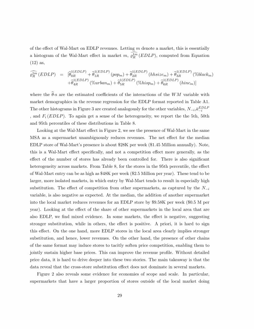
of the e¤ect of Wal-Mart on EDLP revenues. Letting m denote a market, this is essentially
a histogram of the Wal-Mart e¤ect in market m, d%1mR (EDLP ), computed from Equation
(12) as,
d%1mR (EDLP ) = [b�1(EDLP )0R + b�1(EDLP )1R (popm) + b�1(EDLP )2R (hhsizem) + b�1(EDLP )3R (%blackm)
+b�1(EDLP )4R (%urbanm) + b�1(EDLP )5R (%hispm) + b�1(EDLP )6R (hincm)]
where the b�-s are the estimated coe¢ cients of the interactions of the WM variable with
market demographics in the revenue regression for the EDLP format reported in Table A1.
The other histograms in Figure 3 are created analogously for the other variables, N�i,�aEDLP�i
, and Fi (EDLP ). To again get a sense of the heterogeneity, we report the the 5th, 50th
and 95th percentiles of these distributions in Table 8.
Looking at the Wal-Mart e¤ect in Figure 2, we see the presence of Wal-Mart in the same
MSA as a supermarket unambiguously reduces revenues. The net e¤ect for the median
EDLP store of Wal-Mart�s presence is about $28K per week ($1.45 Million annually). Note,
this is a Wal-Mart e¤ect speci�cally, and not a competition e¤ect more generally, as the
e¤ect of the number of stores has already been controlled for. There is also signi�cant
heterogeneity across markets. From Table 8, for the stores in the 95th percentile, the e¤ect
of Wal-Mart entry can be as high as $48K per week ($2.5 Million per year). These tend to be
larger, more isolated markets, in which entry by Wal-Mart tends to result in especially high
substitution. The e¤ect of competition from other supermarkets, as captured by the N�i
variable, is also negative as expected. At the median, the addition of another supermarket
into the local market reduces revenues for an EDLP store by $9.58K per week ($0.5 M per
year). Looking at the e¤ect of the share of other supermarkets in the local area that are
also EDLP, we �nd mixed evidence. In some markets, the e¤ect is negative, suggesting
stronger substitution, while in others, the e¤ect is positive. A priori, it is hard to sign
this e¤ect. On the one hand, more EDLP stores in the local area clearly implies stronger
substitution, and hence, lower revenues. On the other hand, the presence of other chains
of the same format may induce stores to tacitly soften price competition, enabling them to
jointly sustain higher base prices. This can improve the revenue pro�le. Without detailed
price data, it is hard to drive deeper into these two stories. The main takeaway is that the
data reveal that the cross-store substitution e¤ect does not dominate in several markets.
Figure 2 also reveals some evidence for economies of scope and scale. In particular,
supermarkets that have a larger proportion of stores outside of the local market doing
29

EDLP, also tend to earn more under EDLP. This e¤ect is fairly large. At the median, the
economies add about $7.9K per week ($0.4M per year) to revenues. These economies may
arise from the fact that large chains may commit to doing EDLP across many markets (i.e.
a size e¤ect), or from the fact that doing EDLP across many markets may signal a consistent
price image that has spillovers across markets (a scope e¤ect). There is also evidence of
fairly large size/scope e¤ects (signi�cant mass in the right tail), presumably re�ecting the
higher revenues earned by the largest chains.
Figure 3 presents analogous histograms for these e¤ects on revenues under PROMO
pricing. It is interesting to compare the numbers for the e¤ects on PROMO revenues to the
e¤ects on revenues under EDLP. The e¤ect of having a Wal-Mart in the MSA on revenues
under PROMO is also negative as expected, but signi�cantly lower than for EDLP. At the
median, the e¤ect is a $11.98K reduction in PROMO revenues per week ($0.62M annually).
Comparing this to the e¤ect of Wal-Mart presence for EDLP stores, we see Wal-Mart has
a 133% larger e¤ect on EDLP supermarket revenues than PROMO ($1.48M compared to
$0.62M). Clearly, the EDLP positioning of Wal-Mart leads to stronger substitution with
other EDLP stores in the local area, than with other PROMO stores. Also interesting is the
di¤erence between PROMO and EDLP in terms of scale and scope economies. Looking at
Figure 3, we see that there is not as much evidence for such economies on the revenue side
when doing PROMO. This is not very surprising, as promotional polices vary signi�cantly
across geographies in terms of the depth, frequency and magnitude of sales. A PROMO
store in a rural market may use price cycles of di¤erent duration and depth than a PROMO
store in an urban market, re�ecting the nature of underlying demand, which a¤ects its
price discrimination policy. This heterogeneity within the PROMO class contrasts with
the relatively higher uniformity in pricing across geographies under EDLP. Hence, we may
expect that communicating a uniform country-wide price image is easier under EDLP than
under PROMO. This may be one reason to expect spillovers arising from price-image to be
lower under PROMO than under EDLP. Finally, Figure 3 also indicates that the remaining
competition variables do not have signi�cant bite in explaining the revenues di¤erences
across markets under PROMO.
6.2 Costs
We now discuss the results on the cost-side of the model. We organize the discussion along
similar lines to the revenue side, presenting histograms of totals �rst, and then of individual
30

e¤ects across markets. Complete estimation results are presented in Tables A3 and A4 in
the appendix.
Figure 4 presents histograms of the total �xed costs incurred by incumbent supermarkets
under EDLP and PROMO. Analogously, Table 9 presents the 5th, 50th and 95th percentiles
of these costs distributions. How should we interpret these costs? First, note that the �xed
costs are estimated relative to the value of exiting, which has been normalized to zero. A
negative �xed cost estimate indicates the scrap value from exit was higher than incurring
the �xed cost from continued operation under that particular pricing format. Second, the
revenue data are in $1000-s per week. Hence, the �xed costs should be interpreted in the
same units. At the same time, the discrete-choice model is estimated for data on two periods
(1994 and 1998) that are separated by 4 years. Thus, the one-time switching costs should
be thought of as borne over the 4 year window.
Looking at Figure 4 and Table 9, we see the median �xed cost is $173.4K per week under
EDLP ($9M annually), and $401.4K per week ($20M annually) for PROMO stores. Note,
this cannot be compared directly to the median revenues reported in Table 8 because the
median store-market for the revenue distribution is not the same as the median store-market
for the cost distribution. If we compute the true implied gross margins from these estimates,
we �nd that the median gross (or �fully loaded�) margin under EDLP is 12.16% EDLP and
16.5% for PROMO. This is consistent with anecdotal evidence for the supermarket industry.
Table 9 also reports the switching costs estimates. We estimate the median cost of
switching from EDLP to PROMO as $179.1K per week, which works out to be about $37M
over a 4 year horizon. We estimate the median cost of switching from PROMO to EDLP
to be much larger, $860.2K per week, which works out to be about $178M over a 4 year
horizon. This is about 4 times higher than the switch from EDLP to PROMO. In order to
understand the relative comparison of the �xed costs to the switching costs, note the scale
of the �xed costs and the switching costs should be expected to be di¤erent: the �xed costs
are scaled in relation to the revenue from staying relative to exit, while the switching costs
are scaled relative to the present-discounted revenues from staying relative to exit. This
aspect, along with the fact that the model has to rationalize the fact that there are a large
number of switches from EDLP to PROMO, but few from PROMO to EDLP, imply large
switching costs.
We now explore heterogeneity in �xed and switching costs across stores and markets.
Analogous to the revenue results, we report in Figures 5 histograms across markets of the
31
e¤ect of Wal-Mart, the share of competitors doing EDLP, as well as the �EDLP focus�
of the supermarket on �xed costs. Also reported is the distribution of estimated costs of
switching to EDLP across markets. Figure 6 reports the same constructs for the costs of
doing PROMO.
Looking at Figure 5, we �nd that the presence of Wal-Mart in the supermarket�s MSA
reduces �xed costs of operation for the EDLP format. One interpretation of this result is
that the presence of Wal-Mart lowers the costs of marketing an EDLP price positioning in a
local market. For instance, the presence of a Wal-Mart drives tra¢ c into the local market,
which reduces the costs of doing week by week advertising. Another interpretation is that
the entry of Wal-Mart e¤ectively educates consumers in the local market about the value
of an EDLP positioning. The trade-press reports anecdotal evidence consistent with this
phenomena. For example, when Wegmans (a regional supermarket chain in the northeast)
moved from PROMO to EDLP in anticipation of Wal-Mart�s entry, they made large invest-
ments in advertising and public relations to justify this repositioning to consumers, while
also investing in re-educating and retraining their workforce (at stores and warehouses) to
be attuned with the new strategy.
We also see the e¤ect of the chain�s �focus�is to reduce �xed costs, which is essentially
another manifestation of a scope or scale economy on the cost side. The more the chain
tends to do EDLP across the US, the lower are its operating costs of running an EDLP
supermarket in a local market. This is intuitive and in line with expectations. From Table
9, we see the e¤ect of these scope economies on the cost side are large: at the median of
the distribution, the net e¤ect of chain focus on EDLP positioning is by far the largest
component that reduces the �xed costs of operation.
Looking at the results on the PROMO side in Figure 6, we see the e¤ect of Wal-Mart is
�ipped: the presence of Wal-Mart in the local MSA tends to increase the �xed costs of doing
PROMO. We interpret this as re�ecting marketing and advertising costs associated with
promoting and di¤erentiating the store�s strategy in the face of Wal-Mart�s local presence.
The e¤ect of focus is also consistent with the results for PROMO from the revenue side:
a strong focus on PROMO across the country does not seem to lead to large scale or
scope economies in local markets. Again, since PROMO does not require a high degree of
coordination, these results are intuitive.
We can summarize the results of the structural model as follows. Doing PROMO pro-
vides higher margins and revenues. At the median, PROMO pricing provides an incremental
32
revenue of about $6.4M relative to EDLP. Moreover, the cost of switching from PROMO to
EDLP is estimated to be about 4 times larger than from switching from EDLP to PROMO.
The 1990-s were predicted by some as the decade of the EDLP format. These results add
to our understanding of why EDLP adoption has been much more limited than predicted.
6.3 Counterfactual and Simulations
In what follows, we describe two experiments that highlight the roles played by dynamics
and the presence of Wal-Mart in our results.
6.3.1 Costs and Dynamics
Our model estimates the costs of switching and implementing pricing strategies in a dy-
namic environment. To ascertain the role dynamics play in our analysis, we consider an
alternative estimator that instead treats the decision problem as a static game of incom-
plete information. Essentially, we re-estimate the current model with the discount factor
set to zero. We then ask, to what extent is a static model appropriate to understanding
repositioning decisions?
Under the static approach, �xed costs are estimated to be signi�cantly lower for all �rms
(compared to the dynamic model). To see why, note that under a static model, there is no
continuation value from remaining in the market. Thus, in order to justify the switching
and exit rates observed in the data, given the counterfactual revenues, the estimator drives
the costs of operation estimates down. Stated di¤erently, the cost measures under the static
model are biased downward because they combine the true �xed costs of operation with
the option value of staying, or continuing with the current pricing policy. For a signi�cant
fraction of markets, the �xed costs were in fact estimated to be negative (i.e. the omitted
option value dominated the true costs of operation). These di¤erences indicate that a static
setup is inappropriate for measuring the constructs we are interested in.
An examination of the repositioning costs under the static model is also illuminating.
As with the �xed costs of operation, these numbers are also skewed by the change in the
model assumptions, albeit to a lesser extent. The reason for this is that, even in the static
case, repositioning costs are identi�ed o¤ the switches in the data. The di¤erences across
the EDLP and PROMO estimates provide an interesting case in point. While the cost of
repositioning from PROMO to EDLP is estimated to be about 12.67% lower (than in the
dynamic model), the cost of switching from EDLP to PROMO is estimated to be 18.34%
33
higher. The intuition behind this asymmetry lies in the relative di¤erences in continuation
values conditional on switching formats. Since these are no longer part of the model, the
estimates adjust accordingly. Taken together, the di¤erences between the counterfactual
static model and the proposed dynamic game highlight the importance of dynamics in
assessing operating and switching costs.
6.3.2 What if Wal-Mart was everywhere?
Our data and analysis exploited the impact of Wal-Mart. To further quantify the Wal-Mart
e¤ect, we conducted a simple counterfactual by assuming the current state included the
presence of Wal-Mart in all markets. We then forward-simulated the markets from this
initial state allowing for entry, exit and strategy changes based on the model estimates. We
report the distribution under the steady state.
Our steady state results suggest that adding Wal-Mart to every market starting from
the 1998 conditions does push the world toward EDLP, but not in an overwhelming way.
In particular, the overall e¤ect is of the order of a 20% increase in EDLP adoption across
the entire U.S. (32.78% of active supermarkets chose to be EDLP in the counterfactual
steady state, compared to 27.37% in the data). At the same time, market structure is also
pushed towards higher concentration, as exits in the steady state are around 16.3%, versus
the 15.4% observed in the data. Overall, the e¤ect of Wal-Mart is to move the share of
EDLP higher and to increase the exit rate.
6.4 Discussion
The model, results, counterfactuals and critical discussion have all been focussed on our
current application, but we believe our approach extends beyond the evaluation of pricing
strategy. The framework developed here applies naturally to any setting where �rms make
binding decisions to alter their existing strategies. Our results are also useful in highlighting
the fact that dynamics, strategic interactions and the availability of auxiliary post-game
data (such as revenues, prices and sales) are useful in cleanly articulating the costs of
repositioning.
Our modeling approach has limitations, and is based on assumptions that future research
might aim at relaxing. In particular, we highlight three potential avenues of improvement.
First, the stage game could be extended to accommodate additional structural elements. For
example, Beresteanu, Ellickson, and Misra (2007) employ a Bertrand-Nash stage game that
34

allows them to recover price-cost margins and evaluate changes in consumer surplus. While
we don�t have the appropriate data to a¤ord such a speci�cation here, other researchers
might consider this option in the future. Second, we have focused on local market drivers
of pricing strategy, but incorporated scale and scope economies to capture dependencies
of strategies across markets in a limited way. A signi�cant, but challenging, extension to
the current work would be to fully accommodate the joint choice of pricing strategy across
markets. This would require the solution of a daunting dynamic network game, which is
outside of the scope of our current analysis. Finally, extending our framework to allow for
rich layers of persistent unobserved heterogeneity would an important direction forward.
This is an active area of frontier econometric research. We hope to address some of these
extensions in our future work.
7 Conclusions
This paper has made three contributions. First, we draw attention to three salient features
of repositioning decisions in Marketing: that they involve long-term consequences, require
signi�cant sunk investments, and are dynamic in their impact. We outline how the paradigm
of dynamic games can be used to empirically analyze positioning decisions, and to measure
structural constructs like �rm�s repositioning costs. Second, we cast empirical light on an
age-old question in the Marketing of CPG goods: the costs and bene�ts of doing EDLP
versus PROMO. Despite the signi�cant interest in this topic, a full accounting of the long-
term cost and bene�ts of these strategies remains lacking in the literature. Our estimates
add to the evaluation of either strategy, and also identify the sources of heterogeneity in the
relative attractiveness of either across markets. Third, we add to a growing literature at
the intersection of Marketing and Macroeconomics, that has used microdata to understand
the potential sources of rigidity in �rm�s prices over time. The point we make is that
commitment to an EDLP or PROMO strategy is an important source of long-term rigidity
of prices. This point is missing in the extant literature. We discuss why understanding
this rigidity should be properly treated as a dynamic problem. We measure the �menu
cost�to �rms of changing their long-term pricing strategy, and �nd these to be large and
asymmetric. We hope our current work spurs further interest in the dynamics of pricing
and repositioning in Marketing.
35

References
Aguirregabiria, V., and P. Mira (2007): �Sequential Estimation of Dynamic Discrete
Games,�Econometrica, 75, 1�53.
Ailawadi, K., D. R. Lehmann, and S. A. Neslin (2001): �Market Response to a Major
Policy Change in Marketing Mix: Learning from P&G�s Value Pricing Strategy,�Journal
of Marketing, 65, 44�61.
Anderson, E. T., and D. Simester (2010): �Price Stickiness and Customer Antago-
nism,�Quarterly Journal of Economics, 125, 729�765.
Arcidiacono, P., and P. B. Ellickson (2011): �Practical Methods for Estimation of
Dynamic Discrete Choice Models,�Annual Review of Economics, 3.
Arcidiacono, P., and R. A. Miller (2008): �CCP Estimation of Dynamic Discrete
Choice Models with Unobserved Heterogeneity,�Working paper, Duke University.
Bajari, P., C. L. Benkard, and J. Levin (2007): �Estimating Dynamic Models of
Imperfect Competition,�Econometrica, 75, 1331�1370.
Basker, E., andM. Noel (2009): �The Evolving Food Chain: Competitive E¤ects of Wal-
Mart�s Entry into the Supermarket Industry,� Journal of Economics and Management
Strategy, 18, 977�1009.
Bell, D. R., and C. Hilber (2006): �An Empirical Test of the Theory of Sales: Do
Household Storage Constraints In�uence Consumer and Store Behavior?,�Quantitative
Marketing and Economics, 4, 87�117.
Bell, D. R., and J. Lattin (1998): �Shopping Behavior and Consumer Preference for
Retail Price Format: Why �Large Basket�Shoppers Prefer EDLP,�Marketing Science,
17, 66�88.
Beresteanu, A., P. B. Ellickson, and S. Misra (2007): �The Dynamics of Retail
Oligopoly,�Working Paper: University of Rochester.
Bresnahan, T. F., and P. C. Reiss (1991): �Empirical Models of Discrete Games,�
Journal of Econometrics, 48, 57�82.
36

Campbell, J., and B. Eden (2010): �Rigid Prices: Evidence from U.S. Scanner Data��
Chicago Federal Reserve Working Paper.
Chevalier, J., and A. Kashyap (2011): �Best Prices,�Yale University Working Paper.
Dixit, A., and R. Pindyck (1994): Investment Under Uncertainty. Princeton University
Press.
Draganska, M., M. Mazzeo, and K. Seim (2009): �Beyond Plain Vanilla: Model-
ing Joint Product Assortment and Pricing Decisions,�Quantitative Marketing and Eco-
nomics, 7, 105�146.
Dubé, J.-P., G. J. Hitsch, and P. E. Rossi (2009): �Do Switching Costs Make Markets
Less Competitive?,�Journal of Marketing Research, 46, 435�445.
Eichenbaum, M., N. Jaimovich, and S. Rebelo (Forthcoming): �Reference Prices and
Nominal Rigidities,�American Econonmic Review.
Ellickson, P. B., S. Houghton, and C. Timmins (2010): �Estimating Network
Economies in Retail Chains: A Revealed Preference Approach,�NBER Working Paper
15832.
Ellickson, P. B., and S. Misra (2008a): �Enriching Interactions: Incorporating Revenue
and Cost Data into Static Discrete Games,�Working Paper: University of Rochester.
(2008b): �Supermarket Pricing Strategies,�Marketing Science, 27(5), 811�828.
Ericson, R., and A. Pakes (1995): �Markov-Perfect Industry Dynamics: A Framework
for Empirical Work,�Review of Economic Studies, 62, 53�82.
Hartmann, W. R. (2010): �Demand Estimation with Social Interactions and the Impli-
cations for Targeted Marketing,�Marketing Science, 29, 585�601.
Hartmann, W. R., and V. B. Viard (2008): �Do Frequency Reward Programs Create
Switching Costs? A Dynamic Structural Analysis of Demand in a Reward Program,�
Quantitative Marketing and Economics, 6, 109�137.
Ho, T.-H., C. S. Tang, and D. R. Bell (1998): �Rational Shopping Behavior and the
Option Value of Variable Pricing,�Management Science, 44, 145�160.
37

Hoch, S., X. Dreze, and M. Purk (1994): �EDLP, Hi-Lo, and Margin Arithmetic,�
Journal of Marketing, 58, 16�27.
Holmes, T. (Forthcoming): �The Di¤usion of Wal-Mart and Economies of Density,�
Econometrica.
Hotz, V. J., and R. A. Miller (1993): �Conditional Choice Probabilities and the Esti-
mation of Dynamic Models,�Review of Economic Studies, 60, 497�529.
Jia, P. (2008): �What Happens When Wal-Mart Comes to Town: An Empirical Analysis
of the Discount Retail Industry,�Econometrica, 76, 1263�1316.
Kehoe, P., and V. Midrigan (2010): �Prices Are Sticky After All,� Federal Reserve
Bank of Minneapolis working paper.
Lal, R., and R. Rao (1997): �Supermarket Competition: The Case of Every Day Low
Pricing,�Marketing Science, 16, 60�81.
Matsa, D. (Forthcoming): �Competition and Product Quality in the Supermarket Indus-
try,�Quarterly Journal of Economics.
Mulhern, F. J., and R. P. Leone (1990): �Retail Promotional Advertising: Do the
Number of Deal Items and Size of Deal Discounts A¤ect Store Performance?,� Journal
of Business Research, 21, 179�194.
Orhun, Y. (2006): �Spatial Di¤erentiation in the Supermarket Industry,�Working Paper:
University of Chicago Booth School of Business.
Pakes, A., M. Ostrovsky, and S. Berry (2007): �Simple Estimators for the Parame-
ters of Discrete Dynamic Games (with Entry/Exit Examples),�The RAND Journal of
Economics, 38, 373�399.
Pakes, A., J. Porter, K. Ho, and J. Ishii (2005): �Moment Inequalities and Their
Applications,�Working Paper: Harvard University.
Pesendorfer, M. (2002): �Retail Sales: A Study of Pricing Behavior in Supermarkets,�
Journal of Business, 75, 33�66.
Pesendorfer, M., and P. Schmidt-Dengler (2008): �Asymptotic Least Squares Esti-
mators for Dynamic Games,�Review of Economic Studies, 75, 901�928.
38

Roy, R., P. K. Chintagunta, and S. Haldar (1996): �A Framework for Investigating
Habits, �The Hand of the Past,�and Heterogeneity in Dynamic Brand Choice,�Market-
ing Science, 15, 280�299.
Salop, S., and J. E. Stiglitz (1982): �The Theory of Sales: A Simple Model of Equi-
librium Price Dispersion with Identical Agents,�American Economic Review, 72, 1121�
1130.
Singh, V., K. Hansen, and R. Blattberg (2006): �Market Entry and Consumer Be-
havior: An Investigation of a Wal-Mart Supercenter,�Marketing Science, 25, 457�476.
Sobel, J. (1984): �The Timing of Sales,�Review of Economic Studies, L1, 353�368.
Sweeting, A. (2007): �Dynamic Product Positioning in Di¤erentiated Product Industries:
The E¤ect of Fees for Musical Performance Rights on the Commercial Radio Industry,�
Working Paper: Duke University.
Varian, H. R. (1980): �A Model of Sales,�American Economic Review, 70, 651�659.
Vitorino, M. A. (2007): �Empirical Entry Games with Complementarities: An Applica-
tion to the Shopping Center Industry,�Working Paper: University of Pennsylvania.
Zhu, T., and V. Singh (2009): �Spatial Competition and Endogenous Location Choices:
An Application to Discount Retailing,�Quantitative Marketing and Economics, 7, 1�35.
39
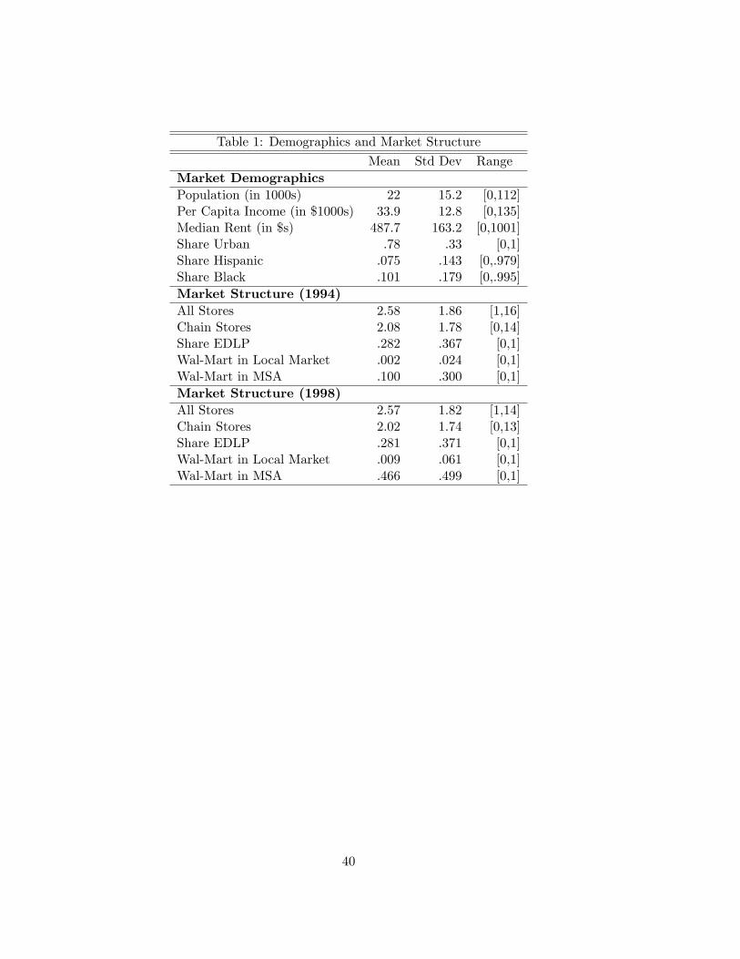
Table 1: Demographics and Market Structure
Mean Std Dev RangeMarket DemographicsPopulation (in 1000s) 22 15.2 [0,112]Per Capita Income (in $1000s) 33.9 12.8 [0,135]Median Rent (in $s) 487.7 163.2 [0,1001]Share Urban .78 .33 [0,1]Share Hispanic .075 .143 [0,.979]Share Black .101 .179 [0,.995]Market Structure (1994)All Stores 2.58 1.86 [1,16]Chain Stores 2.08 1.78 [0,14]Share EDLP .282 .367 [0,1]Wal-Mart in Local Market .002 .024 [0,1]Wal-Mart in MSA .100 .300 [0,1]Market Structure (1998)All Stores 2.57 1.82 [1,14]Chain Stores 2.02 1.74 [0,13]Share EDLP .281 .371 [0,1]Wal-Mart in Local Market .009 .061 [0,1]Wal-Mart in MSA .466 .499 [0,1]
40

Table 2: Store Level Characteristics
All Stores (1994) Exitors OnlyStore Characteristics (1994) Mean Std Dev Range Mean Std Dev RangeEDLP .292 .455 [0,1] .299 .458 [0,1]Sales Volume (in $1000s per week) 239.2 142.8 [57,615] 166.7 105.7 [57,615]Size (in 1000s of sq.ft.) 31.4 16.2 [2,99] 25.1 13.2 [3,99]Stores in Chain 568.4 667.8 [10,2051] 362.8 545.3 [10,2051]Average Size, Stores in Chain 30.6 10.3 [3,99] 27.1 9.9 [3,97]Vertical Integration .652 .476 [0,1] .599 .490 [0,1]
All Stores (1998) Entrants OnlyStore Characteristics (1998)EDLP .287 .452 [0,1] .400 .490 [0,1]Sales Volume (in $1000s per week) 282.2 161.2 [38,691] 297.4 169.9 [38,691]Size (in 1000s of sq.ft.) 33.9 16 [2,190] 38.3 18.4 [4,190]Stores in Chain 701.2 761.7 [1,2316] 703.4 750.1 [1,2316]Average Size, Stores in Chain 33.05 9.67 [2,110] 32.8 11.1 [4,110]Vertical Integration .709 .453 [0,1] .758 .428 [0,1]
41

Table3:Incumbents�Decisions
Counts
PROMO98
EDLP98
EXIT
PROMO94
9314
494
1673
EDLP94
836
3180
715
Probabilities
PROMO98
EDLP98
EXIT
PROMO94
.575
.030
.103
EDLP94
.051
.196
.044
Transitions
PROMO98
EDLP98
EXIT
PROMO94
.811
.043
.146
EDLP94
.177
.672
.151
Table4:Incumbents�Decisions(Wal-Martabsent)
Counts
PROMO98
EDLP98
EXIT
PROMO94
8452
401
1471
EDLP94
774
2784
622
Probabilities
PROMO98
EDLP98
EXIT
PROMO94
.583
.028
.101
EDLP94
.053
.192
.043
Transitions
PROMO98
EDLP98
EXIT
PROMO94
.819
.039
.142
EDLP94
.185
.666
.149
Table5:Incumbents�Decisions(Wal-Martpresent)
Counts
PROMO98
EDLP98
EXIT
PROMO94
862
93202
EDLP94
62396
93
Probabilities
PROMO98
EDLP98
EXIT
PROMO94
.505
.054
.118
EDLP94
.036
.232
.054
Transitions
PROMO98
EDLP98
EXIT
PROMO94
.745
.080
.175
EDLP94
.113
.719
.167
Table6:Entrants�Decisions
Counts
AllMarkets
Wal-MartIn
Wal-MartOut
PROMO98
1191
644
547
EDLP98
795
482
313
Probabilities
PROMO98
.60
.57
.64
EDLP98
.40
.43
.36
42

Table7:DescriptivePolicyFunctions
DependentVariable
P(SwitchjX)P(ExitjX)P(EnterjX)P(EDLPjX)P(EnterjX)
Wal-Martinlocalmarket
:025
(:016)
:027
(:019)
�:141
(:041)
:020
(:104)
Wal-MartinMSA
:017
(:006)
:054
(:008)
:035
(:014)
:053
(:039)
EDLP(thisstore)
:136
(:008)
�:023
(:008)
ShareofEDLP(inlocalmarket)
:010
(:009)
�:002
(:010)
:005
(:008)
:252
(:034)
:021
(:005)
NumberofRivalStores
:0008
(:0016)
:005
(:002)
�:024
(:004)
:009
(:007)
:019
(:003)
TotalOwnStores(allmarkets)
�:0000238
(:000004)
�:000065
(:00004)
Focus
�:342
(:035)
�:151
(:002)
Allregressionsincludeadditionalmarket,storeandchaincontrols
43
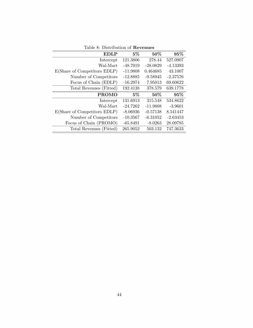
Table 8: Distribution of RevenuesEDLP 5% 50% 95%
Intercept 121.3806 278.44 527.0907Wal-Mart -48.7019 -28.0829 -4.13393
E(Share of Competitors EDLP) -11.9808 0.464685 43.1007Number of Competitors -12.8885 -9.58945 -2.37576Focus of Chain (EDLP) -16.2974 7.95013 69.60622Total Revenues (Fitted) 192.4138 378.579 639.1778
PROMO 5% 50% 95%Intercept 131.6913 315.548 534.8622Wal-Mart -24.7262 -11.9808 -3.9601
E(Share of Competitors EDLP) -8.06936 -0.57138 8.541447Number of Competitors -10.3567 -6.31052 -2.63453
Focus of Chain (PROMO) -65.8491 -8.0263 28.09785Total Revenues (Fitted) 265.9052 503.132 747.3633
44

Table 9: Distribution of CostsEDLP 5% 50% 95%
Intercept 104.9 299.1 426.7Wal-Mart -188.4 -1.1 16.8
E(Share of Competitors EDLP) -27.5 18.0 64.5Focus of Chain (EDLP) -345.3 -126.2 -48.5
Total Fixed Costs (for Non-switchers) 126.34 338.98 1068.28
PROMO 5% 50% 95%Intercept 288.1 417.6 524.9Wal-Mart 62.4 76.0 128.2
E(Share of Competitors EDLP) 24.9 57.8 98.1Focus of Chain (EDLP) -264.3 -32.6 38.8
Total Fixed Costs (for Non-switchers) 320.17 471.64 645.65
Switching Cost (EDLP to PROMO) 102.8 179.1 353.5Switching Cost (PROMO to EDLP) 626.2 860.2 963.2
Counterfactual Revenues - EDLP
Frequency
0 200 400 600 800 1000
01000
2000
Counterfactual Revenues - PROMO
Frequency
200 400 600 800 1000
01000
2000
Figure 1: Counterfactual Revenues
45

Intercept
Frequency
0 500 1000 1500 20000
500
1500
WalMart in MSA
Frequency
-80 -60 -40 -20 0 20
0400
800
E(Share of competitors doing EDLP)
Frequency
0 50 100
0500
1000
1500
Number of Competing Stores
Frequency
-15 -10 -5 0 5
0400
800
1200
Focus of Chain - EDLP
Frequency
-50 0 50 100 150 200
0500
1000
Figure 2: Revenue Components of EDLPIntercept
Frequency
0 500 1000 1500
01000
2000
3000
WalMart in MSA
Frequency
-50 -40 -30 -20 -10 0
01000
2500
E(Share of competitors doing EDLP)
Frequency
-30 -20 -10 0 10 20
01000
3000
Number of Competing Stores
Frequency
-15 -10 -5 0
0500
1000
1500
Focus of Chain - PROMO
Frequency
-250 -200 -150 -100 -50 0 50 100
01000
3000
Figure 3: Revenue Components of PROMO
46

EDLP
Frequency
-500 0 500 10000
200
400
600
PROMO
Frequency
0 500 1000
0500
1500
Figure 4: Estimated Fixed Costs
47

Intercept
Frequency
-100 0 100 200 300 400 500 600
01000
2000
3000
4000
WalMart in MSA
Frequency
-300 -250 -200 -150 -100 -50 0 50
02000
4000
6000
8000
E(Share of competitors doing EDLP)
Frequency
-150 -100 -50 0 50 100 150 200
01000
3000
5000
Focus of Chain - EDLP
Frequency
-600 -500 -400 -300 -200 -100 0 100
02000
4000
6000
Switching Cost
Frequency
400 600 800 1000
01000
2000
3000
4000
Figure 5: Cost Components of EDLP
48

Intercept
Frequency
200 400 600 800
01000
3000
WalMart in MSA
Frequency
20 40 60 80 100 120 140
02000
4000
6000
8000
E(Share of competitors doing EDLP)
Frequency
-50 0 50 100 150
01000
2000
3000
Focus of Chain - PROMO
Frequency
-400 -300 -200 -100 0 100 200 300
01000
3000
5000
Switching Cost
Frequency
100 200 300 400
0500
1500
2500
Figure 6: Cost Components of PROMO
49

APPENDIXTable A1: Revenues from EDLP - Estimates
Variable Interactions Estimate Std. ErrorIntercept Constant -0.6523 35.5339
pop 0.0016 0.0003hhsize -24.4438 12.7931
p_black -102.6822 27.4781p_urban 35.2325 15.5310p_hisp -108.2099 45.5064h_inc 0.0022 0.0004size 7.5916 0.1638
Tstores -0.0023 0.0021Wal-Mart Constant 37.1605 21.9720
pop 0.0000 0.0002hhsize -9.0415 8.8520
p_black 6.4417 16.6351p_urban -31.8804 11.2913p_hisp 40.9846 28.0828h_inc -0.0006 0.0003
E(Comp EDLP) Constant -7.1783 34.7848pop -0.0005 0.0003
hhsize 3.4141 14.4438p_black 8.4550 23.5232p_urban 9.6604 12.8207p_hisp 136.0845 40.8996h_inc 0.0000 0.0005
Focus EDLP Constant -110.6356 40.6572pop -0.0006 0.0003
hhsize 50.0621 14.0387p_black 19.4849 24.9504p_urban 25.5088 17.5207p_hisp 122.4777 39.6719h_inc -0.0008 0.0006
Number of Competing Constant 1.1957 7.4977Stores pop 0.0000 0.0000
hhsize -3.6288 2.7348p_black 16.0630 3.8475p_urban -2.3297 2.6031p_hisp 16.0160 8.7817h_inc 0.0000 0.0001
50
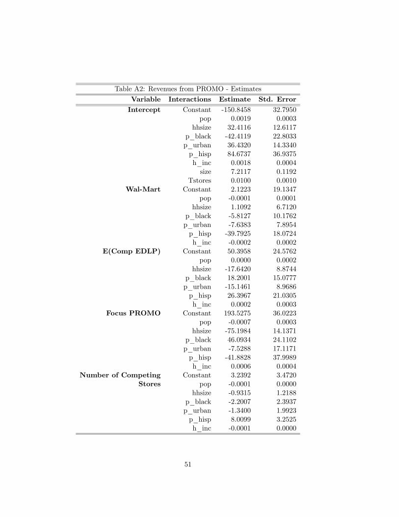
Table A2: Revenues from PROMO - Estimates
Variable Interactions Estimate Std. ErrorIntercept Constant -150.8458 32.7950
pop 0.0019 0.0003hhsize 32.4116 12.6117
p_black -42.4119 22.8033p_urban 36.4320 14.3340p_hisp 84.6737 36.9375h_inc 0.0018 0.0004size 7.2117 0.1192
Tstores 0.0100 0.0010Wal-Mart Constant 2.1223 19.1347
pop -0.0001 0.0001hhsize 1.1092 6.7120
p_black -5.8127 10.1762p_urban -7.6383 7.8954p_hisp -39.7925 18.0724h_inc -0.0002 0.0002
E(Comp EDLP) Constant 50.3958 24.5762pop 0.0000 0.0002
hhsize -17.6420 8.8744p_black 18.2001 15.0777p_urban -15.1461 8.9686p_hisp 26.3967 21.0305h_inc 0.0002 0.0003
Focus PROMO Constant 193.5275 36.0223pop -0.0007 0.0003
hhsize -75.1984 14.1371p_black 46.0934 24.1102p_urban -7.5288 17.1171p_hisp -41.8828 37.9989h_inc 0.0006 0.0004
Number of Competing Constant 3.2392 3.4720Stores pop -0.0001 0.0000
hhsize -0.9315 1.2188p_black -2.2007 2.3937p_urban -1.3400 1.9923p_hisp 8.0099 3.2525h_inc -0.0001 0.0000
51

Table A3: Costs of EDLP Strategy - EstimatesVariable Interactions Estimate Std. ErrorIntercept Constant -133.8927 55.3286
pop 0.0003 0.0004hhsize 43.8758 20.4330
p_black 13.1109 37.9669p_urban 253.5417 23.2904p_hisp 97.0457 58.5680h_inc 0.0030 0.0005size 0.7551 0.1154
Tstores -0.0643 0.0023VI 6.5339 3.2142
Wal-Mart Constant 29.8790 58.3165pop -0.0001 0.0005
hhsize -2.3037 18.6033p_black 21.7578 36.3507p_urban -1.8997 30.6304p_hisp -110.5341 47.2392h_inc -0.0004 0.0006
E(Comp EDLP) Constant 204.5877 47.1675pop 0.0015 0.0004
hhsize -64.5469 19.2611p_black -4.8201 29.1064p_urban -65.7558 18.0506p_hisp 71.9132 38.9716h_inc 0.0000 0.0005
Focus EDLP Constant 175.5205 71.2307pop 0.0000 0.0005
hhsize -127.7017 25.9529p_black 149.7402 47.9211p_urban -22.0618 27.9735p_hisp -45.6229 69.0855h_inc 0.0019 0.0007
Switching Costs Constant 1242.8909 47.2055pop 0.0004 0.0003
hhsize -99.5798 17.4759p_black -265.9400 33.0221p_urban -36.4333 20.0746p_hisp -96.7333 49.3402h_inc -0.0003 0.0004
Wal-Mart in MSA -182.2738 10.7021E(Comp EDLP) -22.7443 9.1154
Focus EDLP -202.6674 13.0266
52
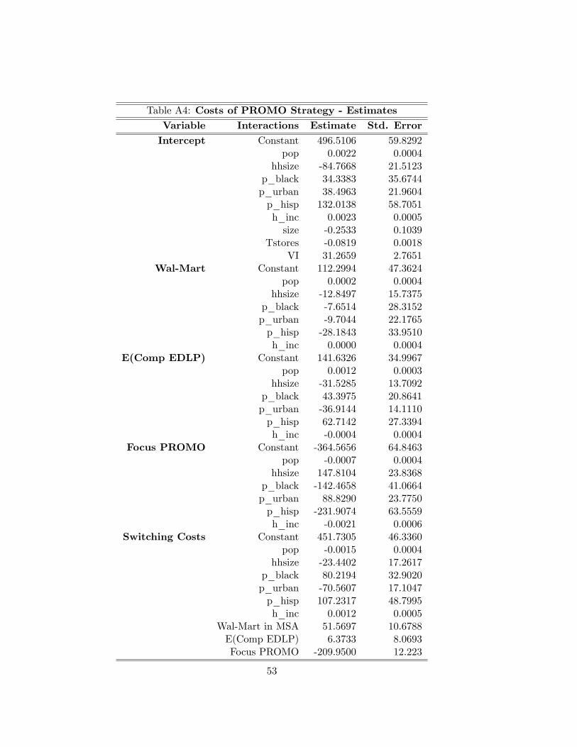
Table A4: Costs of PROMO Strategy - EstimatesVariable Interactions Estimate Std. ErrorIntercept Constant 496.5106 59.8292
pop 0.0022 0.0004hhsize -84.7668 21.5123
p_black 34.3383 35.6744p_urban 38.4963 21.9604p_hisp 132.0138 58.7051h_inc 0.0023 0.0005size -0.2533 0.1039
Tstores -0.0819 0.0018VI 31.2659 2.7651
Wal-Mart Constant 112.2994 47.3624pop 0.0002 0.0004
hhsize -12.8497 15.7375p_black -7.6514 28.3152p_urban -9.7044 22.1765p_hisp -28.1843 33.9510h_inc 0.0000 0.0004
E(Comp EDLP) Constant 141.6326 34.9967pop 0.0012 0.0003
hhsize -31.5285 13.7092p_black 43.3975 20.8641p_urban -36.9144 14.1110p_hisp 62.7142 27.3394h_inc -0.0004 0.0004
Focus PROMO Constant -364.5656 64.8463pop -0.0007 0.0004
hhsize 147.8104 23.8368p_black -142.4658 41.0664p_urban 88.8290 23.7750p_hisp -231.9074 63.5559h_inc -0.0021 0.0006
Switching Costs Constant 451.7305 46.3360pop -0.0015 0.0004
hhsize -23.4402 17.2617p_black 80.2194 32.9020p_urban -70.5607 17.1047p_hisp 107.2317 48.7995h_inc 0.0012 0.0005
Wal-Mart in MSA 51.5697 10.6788E(Comp EDLP) 6.3733 8.0693Focus PROMO -209.9500 12.223
53


