
RESEARCH Open Access
A half-discrete Hilbert-type inequality witha homogeneous kernel and an extensionBicheng Yang1* and Qiang Chen2
* Correspondence: [email protected] of Mathematics,Guangdong University ofEducation Guangzhou, Guangdong510303, P. R. ChinaFull list of author information isavailable at the end of the article
Abstract
Using the way of weight functions and the technique of real analysis, a half-discreteHilbert-type inequality with a general homogeneous kernel is obtained, and a bestextension with two interval variables is given. The equivalent forms, the operatorexpressions, the reverses and some particular cases are considered.2000 Mathematics Subject Classification: 26D15; 47A07.
Keywords: Hilbert-type inequality, homogeneous kernel, weight function, equivalentform, reverse
1 Introduction
Assuming that p > 1,1p+1q= 1, f (≥ 0) Î Lp (R+), g(≥ 0) Î Lq (R+),
∥∥f∥∥p ={∫ ∞
0f p(x)dx
} 1p
> 0 , || g ||q >0, we have the following Hardy-Hilbert’s integral
inequality [1]:
∞∫0
∞∫0
f (x)g(y)x + y
dxdy <π
sin(π/p)||f ||p||g||q, (1)
where the constant factorπ
sin(π/p) is the best possible. If am, bn ≥ 0,
b = {bn}∞n=1 ∈ lq , b = {bn}∞n=1 ∈ lq , ||a||p ={∑∞
m=1apm
} 1p
> 0 , || b ||q >0, then we still
have the following discrete Hardy-Hilbert’s inequality with the same best constant fac-
torπ
sin(π/p) :
∞∑m=1
∞∑n=1
ambnm + n
<π
sin(π/p)||a||p||b||q. (2)
For p = q = 2, the above two inequalities reduce to the famous Hilbert’s inequalities.
Inequalities (1) and (2) are important in analysis and its applications [2-4].
In 1998, by introducing an independent parameter l Î (0, 1], Yang [5] gave an
extension of (1) for p = q = 2. Refinement and generalizing the results from [5], Yang
[6] gave some best extensions of (1) and (2) as follows: If l1, l2 Î R, l1 + l2 = l, kl(x,
Yang and Chen Journal of Inequalities and Applications 2011, 2011:124http://www.journalofinequalitiesandapplications.com/content/2011/1/124
© 2011 Yang and Chen; licensee Springer. This is an Open Access article distributed under the terms of the Creative CommonsAttribution License (http://creativecommons.org/licenses/by/2.0), which permits unrestricted use, distribution, and reproduction inany medium, provided the original work is properly cited.

y) is a non-negative homogeneous function of degree - l satisfying for any x, y, t >0, kl
(tx, ty) = t-l kl (x, y), k(λ1) =∫ ∞
0kλ(t, 1)tλ1−1dt ∈ R+ , φ(x) = xp(1−λ1)−1 ,
f (≥ 0) ∈ Lp,φ(R+) = {f |||f ||p,φ := {∫ ∞
0φ(x)|f (x)|pdx}
1p < ∞} ,
f (≥ 0) ∈ Lp,φ(R+) = {f |||f ||p,φ := {∫ ∞
0φ(x)|f (x)|pdx}
1p < ∞} , g(≥ 0) Î Lq,ψ, || f ||p,j, ||
g ||q,ψ >0, then we have
∞∫0
∞∫0
kλ(x, y)f (x)g(y)dxdy < k(λ1)||f ||p,φ ||g||q,ψ , (3)
where the constant factor k(l1) is the best possible. Moreover, if kl(x, y) is finite and
kλ(x, y)xλ1−1(kλ(x, y)yλ2−1) is decreasing with respect to x >0(y >0), then for am,bn ≥
0, a = {am}∞m=1 ∈ lp,φ = {a|||a||p,φ := {∑∞
n=1φ(n)|an|p}
1p < ∞} , b = {bn}∞n=1 ∈ lq,ψ , || a ||
p,j, || b ||q,Ψ >0, we have
∞∑m=1
∞∑n=1
kλ(m,n)ambn < k(λ1)||a||p,φ||b||q,ψ , (4)
with the best constant factor k(l1). Clearly, for l = 1, k1(x, y) =1
x + y, λ1 =
1q,
λ2 =1p(3) reduces to (1), and (4) reduces to (2). Some other results about Hilbert-
type inequalities are provided by [7-15].
On half-discrete Hilbert-type inequalities with the non-homogeneous kernels, Hardy
et al. provided a few results in Theorem 351 of [1]. But they did not prove that the
constant factors are the best possible. And, Yang [16] gave a result by introducing an
interval variable and proved that the constant factor is the best possible. Recently,
Yang [17] gave the following half-discrete Hilbert’s inequality with the best constant
factor B(l1, l2)(l, l1 >0, 0 <l2 ≤ 1, l1 + l2 = l):
∞∫0
f (x)∞∑n=1
an(x + n)λ
dx < B(λ1,λ2)||f ||p,ϕ||a||q,ψ . (5)
In this article, using the way of weight functions and the technique of real analysis, a
half-discrete Hilbert-type inequality with a general homogeneous kernel and a best
constant factor is given as follows:
∞∫0
f (x)∞∑n=1
kλ(x, n)andx < k(λ1)||f ||p,ϕ ||a||q,ψ , (6)
which is a generalization of (5). A best extension of (6) with two interval variables,
some equivalent forms, the operator expressions, the reverses and some particular
cases are considered.
Yang and Chen Journal of Inequalities and Applications 2011, 2011:124http://www.journalofinequalitiesandapplications.com/content/2011/1/124
Page 2 of 16

2 Some lemmasWe set the following conditions:
Condition (i) v(y)(y Î [n0 - 1, ∞)) is strictly increasing with v(n0 - 1) ≥ 0 and for any
fixed x Î (b, c), f(x, y) is decreasing for y Î (n0 - 1, ∞) and strictly decreasing in an
interval of (n0 - 1, ∞).
Condition (ii) v(y)(y ∈ [n0 − 12,∞)) is strictly increasing with v
(n0 − 1
2
)≥ 0 and
for any fixed x Î (b, c), f(x, y) is decreasing and strictly convex for y ∈(n0 − 1
2,∞
).
Condition (iii) There exists a constant b ≥ 0, such that v(y)(y Î [n0 - b, ∞)) is
strictly increasing with v(n0 - b) ≥ 0, and for any fixed x Î (b, c), f(x, y) is piecewise
smooth satisfying
R(x) :=
n0∫n0−β
f (x, y)dy − 12f (x,n0) −
∞∫n0
ρ(y)f ′y(x, y)dy > 0,
where ρ(y)(= y − [y] − 12) is Bernoulli function of the first order.
Lemma 1 If l1, l2 Î R, l1 + l2 = l, kl(x, y) is a non-negative finite homogeneous
function of degree - l in R2+, u(x)(x ∈ (b, c),−∞ ≤ b < c ≤ ∞)and v(y)(y Î [n0, ∞), n0
Î N) are strictly increasing differential functions with u(b+) = 0, v(n0) >0, u(c-) = v(∞)
= ∞, setting K(x, y) = kl(u(x), v(y)), then we define weight functions ω(n) and ϖ(x) as
follows:
ω(n) : = [v(n)]λ2
c∫b
K(x,n)[u(x)]λ1−1u′(x)dx,n ≥ n0(n ∈ N), (7)
(x) : = [u(x)]λ1
∞∑n=n0
K(x,n)[v(n)]λ2−1v′(n), x ∈ (b, c). (8)
It follows
ω(n) = k(λ1) : =
∞∫0
kλ(t, 1)tλ1−1dt. (9)
Moreover, setting f (x, y) : = [u(x)]λ1K(x, y)[v(y)]λ2−1v′(y) , if k(l1) Î R+ and one of the
above three conditions is fulfilled, then we still have
(x) < k(λ1)(x ∈ (b, c)). (10)
Proof. Setting t =u(x)v(n)
in (7), by calculation, we have (9).
Yang and Chen Journal of Inequalities and Applications 2011, 2011:124http://www.journalofinequalitiesandapplications.com/content/2011/1/124
Page 3 of 16

(i) If Condition (i) is fulfilled, then we have
(x) =∞∑
n=n0
f (x,n) < [u(x)]λ1
∞∫n0−1
K(x, y)[v(y)]λ2−1v′(y)dy
t=u(x)/v(y)=
u(x)v(n0−1)∫0
kλ(t, 1)tλ1−1dt ≤ k(λ1).
(ii) If Condition (ii) is fulfilled, then by Hadamard’s inequality [18], we have
(x) =∞∑
n=n0
f (x,n) <
∞∫n0−1
2
f (x, y)dy
t=u(x)/v(y)=
u(x)
v(n0−12 )∫
0
kλ(t, 1)tλ1−1dt ≤ k(λ1).
(iii) If Condition (iii) is fulfilled, then by Euler-Maclaurin summation formula [6], we
have
(x) =∞∑
n=n0
f (x,n)
=
∞∫n0
f (x, y)dy +12f (x,n0)+
∞∫n0
ρ(y)f ′y(x, y)dy
=
∞∫n0−β
f (x, y)dy − R(x)
=
u(x)v(n0 − β)∫
0
kλ(t, 1)tλ1−1dt − R(x)
≤ k(λ1) − R(x) < k(λ1).
The lemma is proved. ■Lemma 2 Let the assumptions of Lemma 1 be fulfilled and additionally, p >0(p ≠ 1),
1p+1q= 1,an ≥ 0, n ≥ n0(n Î N), f (x) is a non-negative measurable function in (b, c).
Then, (i) for p >1, we have the following inequalities:
J1 : =
⎧⎨⎩
∞∑n=n0
v′(n)[v(n)]1−pλ2
⎡⎣ c∫
d
K(x,n)f (x)dx
⎤⎦
p⎫⎬⎭
1p
≤ [k(λ1)]1q
⎧⎨⎩
c∫d
(x)[u(x)]p(1−λ1)−1
[u′(x)]p−1 f p(x)dx
⎫⎬⎭
1p
,
(11)
Yang and Chen Journal of Inequalities and Applications 2011, 2011:124http://www.journalofinequalitiesandapplications.com/content/2011/1/124
Page 4 of 16
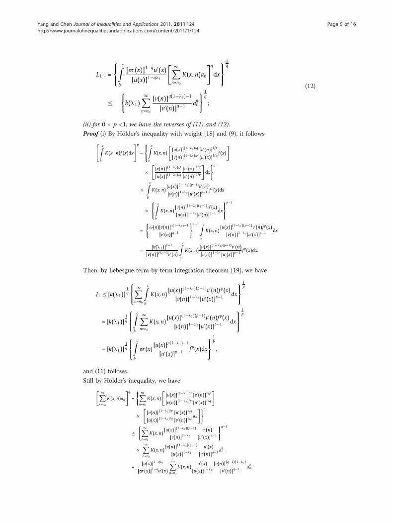
L1 : =
⎧⎨⎩
c∫b
[ (x)]1−qu′(x)[u(x)]1−qλ1
[ ∞∑n=n0
K(x,n)an
]q
dx
⎫⎬⎭
1q
≤{k(λ1)
∞∑n=n0
[v(n)]q(1−λ2)−1
[v′(n)]q−1 aqn
} 1q
;
(12)
(ii) for 0 < p <1, we have the reverses of (11) and (12).
Proof (i) By Hölder’s inequality with weight [18] and (9), it follows
⎡⎣ c∫
b
K(x, n)f (x)dx
⎤⎦
p
=
⎧⎨⎩
c∫b
K(x,n)
[[u(x)](1−λ1)/q
[v(n)](1−λ2)/p
[v′(n)]1/p
[u′(x)]1/qf (x)
]
×[[v(n)](1−λ2)/p
[u(x)](1−λ1)/q
[u′(x)]1/q
[v′(n)]1/p
]dx
}p
≤c∫
b
K(x,n)[u(x)](1−λ1)(p−1)v′(n)[v(n)]1−λ2 [u′(x)]p−1 f p(x)dx
×⎧⎨⎩
c∫b
K(x,n)[v(n)](1−λ2)(q−1)u′(x)[u(x)]1−λ1 [v′(n)]q−1 dx
⎫⎬⎭
p−1
=
{ω(n)[v(n)]q(1−λ2)−1
[v′(n)]q−1
}p−1 c∫b
K(x,n)[u(x)](1−λ1)(p−1)v′(n)f p(x)
[v(n)]1−λ2 [u′(x)]p−1 dx
=[k(λ1)]
p−1
[v(n)]pλ2−1v′(n)
c∫b
K(x,n)[u(x)](1−λ1)(p−1)v′(n)[v(n)]1−λ2 [u′(x)]p−1 f p(x)dx.
Then, by Lebesgue term-by-term integration theorem [19], we have
J1 ≤ [k(λ1)]1q
⎧⎨⎩
∞∑n=n0
c∫b
K(x,n)[u(x)](1−λ1)(p−1)v′(n)f p(x)
[v(n)]1−λ2 [u′(x)]p−1 dx
⎫⎬⎭
1p
= [k(λ1)]1q
⎧⎨⎩
c∫b
∞∑n=n0
K(x,n)[u(x)](1−λ1)(p−1)v′(n)f p(x)
[v(n)]1−λ2 [u′(x)]p−1 dx
⎫⎬⎭
1p
= [k(λ1)]1q
⎧⎨⎩
c∫b
(x)[u(x)]p(1−λ1)−1
[u′(x)]p−1 f p(x)dx
⎫⎬⎭
1p
,
and (11) follows.
Still by Hölder’s inequality, we have
[ ∞∑n=n0
K(x,n)an
]q
=
{ ∞∑n=n0
K(x,n)
[[u(x)](1−λ1)/q
[v(n)](1−λ2)/p
[v′(n)]1/p
[u′(x)]1/q
]
×[[v(n)](1−λ2)/p
[u(x)](1−λ1)/q
[u′(x)]1/q
[v′(n)]1/pan
]}q
≤{ ∞∑n=n0
K(x,n)[u(x)](1−λ1)(p−1)
[v(n)]1−λ2
v′(n)[u′(x)]p−1
}q−1
×∞∑
n=n0
K(x,n)[v(n)](1−λ2)(q−1)
[u(x)]1−λ1
u′(x)[v′(n)]q−1 a
qn
=[u(x)]1−qλ1
[ (x)]1−qu′(x)
∞∑n=n0
K(x,n)u′(x)
[u(x)]1−λ1
[v(n)](q−1)(1−λ2)
[v′(n)]q−1 aqn.
Yang and Chen Journal of Inequalities and Applications 2011, 2011:124http://www.journalofinequalitiesandapplications.com/content/2011/1/124
Page 5 of 16

Then, by Lebesgue term-by-term integration theorem, we have
L1 ≤⎧⎨⎩
c∫b
∞∑n=n0
K(x,n)u′(x)
[u(x)]1−λ1
[v(n)](q−1)(1−λ2)
[v′(n)]q−1 aqndx
⎫⎬⎭
1q
=
⎧⎨⎩
∞∑n=n0
⎡⎣[v(n)]λ2
c∫b
K(x,n)u′(x)dx
[u(x)]1−λ1
⎤⎦ [v(n)]q(1−λ2)−1
[v′(n)]q−1 aqn
⎫⎬⎭
1q
=
{ ∞∑n=n0
ω(n)[v(n)]q(1−λ2)−1
[v′(n)]q−1 aqn
} 1q
,
and then in view of (9), inequality (12) follows.
(ii) By the reverse Hölder’s inequality [18] and in the same way, for q <0, we have
the reverses of (11) and (12). ■
3 Main results
We set (x) :=[u(x)]p(1−λ1)−1
[u′(x)]p−1 (x ∈ (b, c)) , �(n) :=[v(n)]q(1−λ2)−1
[v′(n)]q−1 (n ≥ n0,n ∈ N) ,
wherefrom [(x)]1−q =u′(x)
[u(x)]1−qλ1, [�(n)]1−p =
v′(n)[v(n)]1−pλ2
.
Theorem 1 Suppose that l1, l2 Î R, l1 + l2 = l, kl(x, y) is a non-negative finite
homogeneous function of degree - l¸ in R2+, u(x)(x ∈ (b, c),−∞ ≤ b < c ≤ ∞) and v(y)
(y Î [n0, ∞), n0 Î N are strictly increasing differential functions with u(b+) = 0, v(n0)
>0, u(c-) = v(∞) = ∞, ϖ(x) < k (l1) Î R+(x Î (b, c)). If p > 1,1p+1q= 1 , f (x), an ≥ 0, f
Î LpF (b, c), a = {an}∞n=n0 ∈ lq,� , || f ||p,F >0 and || a ||q,Ψ > 0, then we have the follow-
ing equivalent inequalities:
I : =∞∑
n=n0
an
c∫b
K(x,n)f (x)dx =
c∫b
f (x)∞∑
n=n0
K(x,n)andx
< k(λ1)||f ||p,||a||q,� ,(13)
J :=
⎧⎨⎩
∞∑n=n0
[�(n)]1−p
⎡⎣ c∫
b
K(x,n)f (x)dx
⎤⎦
p⎫⎬⎭
1p
< k(λ1)||f ||p,, (14)
L :=
⎧⎨⎩
c∫b
[(x)]1−q
[ ∞∑n=n0
K(x,n)an
]q
dx
⎫⎬⎭
1q
< k(λ1)||a||q,� . (15)
Moreover, ifv′(y)v(y)
(y ≥ n0) is decreasing and there exist constants δ < l1 and M >0,
such that kλ(t, 1) ≤ Mtδ
(t ∈
(0,
1v(n0)
]), then the constant factor k(l1) in the above
inequalities is the best possible.
Yang and Chen Journal of Inequalities and Applications 2011, 2011:124http://www.journalofinequalitiesandapplications.com/content/2011/1/124
Page 6 of 16

Proof By Lebesgue term-by-term integration theorem, there are two expressions for I in
(13). In view of (11), for ϖ(x) < k(l1) Î R+, we have (14). By Hölder’s inequality, we have
I =∞∑
n=n0
⎡⎣�
−1q(n)
c∫b
K(x, n)f (x)dx
⎤⎦ [�
1q (n)an] ≤ J||a||q,� . (16)
Then, by (14), we have (13). On the other hand, assuming that (13) is valid, setting
an := [�(n)]1−p
⎡⎣ c∫
b
K(x, n)f (x)dx
⎤⎦
p−1
,n ≥ n0,
then Jp-1 = || a ||q,Ψ . By (11), we find J <∞. If J = 0, then (14) is naturally valid; if J
>0, then by (13), we have
||a||qq,� = Jp = I < k(λ1)||f ||p,||a||q,� , ||a||q−1q,� = J < k(λ1)||f ||p,,
and we have (14), which is equivalent to (13).
In view of (12), for [ϖ(x) ]1-q >[k(l1)]1-q, we have (15). By Hölder’s in equality, we find
I =
c∫b
[1p (x)f (x)]
[
−1p (x)
∞∑n=n0
K(x,n)an
]dx ≤ ||f ||p,L. (17)
Then, by (15), we have (13). On the other hand, assuming that (13) is valid, setting
f (x) := [(x)]1−q
[ ∞∑n=n0
K(x,n)an
]q−1
, x ∈ (b, c),
then Lq-1 = || f ||pF . By (12), we find L <∞. If L = 0, then (15) is naturally valid; if L
>0, then by (13), we have
||f ||pp, = Lq = I < k(λ1)||f ||p,||a||q,� , ||f ||p−1p, = L < k(λ1)||a||q,� ,
and we have (15) which is equivalent to (13).
Hence, inequalities (13), (14) and (15) are equivalent.
There exists an unified constant d Î (b, c), satisfying u(d) = 1. For 0 < ε < p(l1 - δ),
setting f (x) = 0 , x Î (b, d); f (x) = [u(x)]λ1− ε
p−1u′(x), x Î (d, c), and
an = [v(n)]λ2− ε
q−1v′(n) , n ≥ n0, if there exists a positive number k(≤ k(l1)), such that
(13) is valid as we replace k(l1) by k, then in particular, we find
I : =∞∑
n=n0
c∫b
K(x,n)an f (x)dx < k||f ||p,||a||q,�
= k
⎧⎨⎩
c∫d
u′(x)[u(x)]ε+1
dx
⎫⎬⎭
1p⎧⎨⎩ v′(n0)[v(n0)]
ε+1 +∞∑
n=n0+1
v′(n)[v(n)]ε+1
⎫⎬⎭
1q
< k(1ε
)1p
⎧⎨⎩ v′(n0)[v(n0)]
ε+1 +
∞∫n0
[v(y)]−ε−1v′(y)dy
⎫⎬⎭
1q
=kε
{ε
v′(n0)[v(n0)]
ε+1 + [v(n0)]−ε
} 1q
(18)
Yang and Chen Journal of Inequalities and Applications 2011, 2011:124http://www.journalofinequalitiesandapplications.com/content/2011/1/124
Page 7 of 16

I =∞∑
n=n0
[v(n)]λ2− ε
q−1v′(n)
c∫d
K(x,n)[u(x)]λ1− ε
p−1u′(x)dx
t=u(x)/v(n)=
∞∑n=n0
[v(n)]−ε−1v′(n)
∞∫1/v(n)
kλ(t, 1)tλ1− ε
p−1dt
= k(
λ1 − ε
p
) ∞∑n=n0
[v(n)]−ε−1v′(n) − A(ε)
> k(
λ1 − ε
p
) ∞∫n0
[v(y)]−ε−1v′(y)dy − A(ε)
=1εk(
λ1 − ε
p
)[v(n0)]−ε − A(ε),
A(ε) : =∞∑
n=n0
[v(n)]−ε−1v′(n)
1/v(n)∫0
kλ(t, 1)tλ1− ε
p−1dt.
(19)
For kλ(t, 1) ≤ M(1tδ
)(δ < λ1; t ∈ (0, 1/v(n0)]) , we find
0 < A(ε) ≤ M∞∑
n=n0
[v(n)]−ε−1v′(n)
1/v(n)∫0
tλ1−δ− ε
p−1dt
=M
λ1 − δ − εp
∞∑n=n0
[v(n)]−λ1+δ− ε
q−1v′(n)
=M
λ1 − δ − ε
p
⎡⎣ v′(n0)
[v(n0)]λ1−δ+ ε
q +1+
∞∑n=n0+1
v′(n)
[v(n)]λ1−δ+ ε
q +1
⎤⎦
≤ M
λ1 − δ − ε
p
⎡⎣ v′(n0)
[v(n0)]λ1−δ+ ε
q +1+
∞∫n0
v′(y)
[v(y)]λ1−δ+ ε
q +1dy
⎤⎦
=M
λ1 − δ − ε
p
⎡⎣ v′(n0)
[v(n0)]λ1−δ+ ε
q +1+[v(n0)]
−λ1+δ− εq
λ1 − δ + εq
⎤⎦ < ∞,
namely A(ε) = O(1)(ε ® 0+). Hence, by (18) and (19), it follows
k(
λ1 − ε
p
)[v(n0)]−ε − εO (1) < k
{ε
v′(n0)[v(n0)]
ε+1 + [v(n0)]−ε
} 1q. (20)
By Fatou Lemma [19], we have k(λ1) ≤ limε→0+ k(
λ1 − ε
p
), then by (20), it follows
k(l1) ≤ k(ε ® 0+). Hence, k = k(l1) is the best value of (12).
By the equivalence, the constant factor k(l1) in (14) and (15) is the best possible,
otherwise we can imply a contradiction by (16) and (17) that the constant factor in
(13) is not the best possible. ■
Yang and Chen Journal of Inequalities and Applications 2011, 2011:124http://www.journalofinequalitiesandapplications.com/content/2011/1/124
Page 8 of 16

Remark 1 (i) Define a half-discrete Hilbert’s operator T : Lp,(b, c) → lp,�1−p as: for f
Î LpF (b, c), we define Tf ∈ lp,�1−p , satisfying
Tf (n) =
c∫b
K(x,n)f (x)dx, n ≥ n0.
Then, by (14), it follows ||Tf ||p.�1−p ≤ k(λ1)||f ||p, and then T is a bounded operator
with || T || ≤ k(l1). Since, by Theorem 1, the constant factor in (14) is the best possi-
ble, we have || T || = k(l1).
(ii) Define a half-discrete Hilbert’s operator T : lq,� → Lq,1−q(b, c) as: for a Î lqΨ ,
we define Ta ∈ Lq,1−q(b, c) , satisfying
Ta(x) =∞∑
n=n0
K(x,n)an, x ∈ (b, c).
Then, by (15), it follows ||Ta||q,1−q ≤ k(λ1)||a||q,� and then T is a bounded opera-
tor with ||T|| ≤ k(λ1) . Since, by Theorem 1, the constant factor in (15) is the best pos-
sible, we have ||T|| = k(λ1) .
In the following theorem, for 0 < p <1, or p <0, we still use the formal symbols of
||f ||p, and ||a||q,Ψ and so on. ■Theorem 2 Suppose that l1, l2 Î R, l1 + l2 = l, kl(x, y) is a non-negative finite homo-
geneous function of degree -l in R2+ , u(x)(x Î (b, c), -∞ ≤ b < c ≤ ∞) and v(y)(y Î [n0, ∞),
n0 Î N) are strictly increasing differential functions with u(b+) = 0, v(n0) >0, u(c-) = v(∞) =
∞, k(l1) Î R+, θl(x) Î (0, 1), k(l1)(1 - θl(x)) <ϖ(x) <k(l1)(x Î (b, c)). If 0 < p <1,1p +
1q = 1 , f(x), an ≥ 0, (x) := (1 − θλ(x))(x)(x ∈ (b, c)) , 0 < ||f ||q, < ∞and 0 <||
a||q,Ψ < ∞. Then, we have the following equivalent inequalities:
I : =∞∑
n=n0
c∫b
K(x,n)anf (x)dx =
c∫b
∞∑n=n0
K(x,n)anf (x)dx
> k(λ1)||f ||p,||a||q,� ,(21)
J :=
⎧⎨⎩
∞∑n=n0
[�(n)]1−p
⎡⎣ c∫
b
K(x,n)f (x)dx
⎤⎦
p⎫⎬⎭
1p
> k(λ1)||f ||p,, (22)
L :=
⎧⎨⎩
c∫b
[(x)]1−q
[ ∞∑n=n0
K(x,n)an
]q
dx
⎫⎬⎭
1q
> k(λ1)||a||q,� . (23)
Moreover, if v′(y)v(y) (y ≥ n0) is decreasing and there exist constants δ, δ0 >0, such that
θλ(x) = O( 1[u(x)]δ
)(x ∈ (d, c))and k(l1 - δ0) Î R+, then the constant factor k(l1) in the
above inequalities is the best possible.
Yang and Chen Journal of Inequalities and Applications 2011, 2011:124http://www.journalofinequalitiesandapplications.com/content/2011/1/124
Page 9 of 16

Proof. In view of (9) and the reverse of (11), for ϖ(x) > k(l1)(1 - θl(x)), we have (22).
By the reverse Hölder’s inequality, we have
I =∞∑
n=n0
⎡⎣�
−1q (n)
c∫b
K(x,n)f (x)dx
⎤⎦ [�
1q (n)an] ≥ J||a||q,� . (24)
Then, by (22), we have (21). On the other hand, assuming that (21) is valid, setting
an as Theorem 1, then Jp-1 = ||a||qΨ. By the reverse of (11), we find J >0. If J = ∞, then
(24) is naturally valid; if J <∞, then by (21), we have
||a||qq,� = Jp = I > k(λ1)||f ||p,||a||q,� , ||a||q−1q,� = J > k(λ1)||f ||p,,
and we have (22) which is equivalent to (21).
In view of (9) and the reverse of (12), for [ϖ(x)]1-q >[k(l1)(1 - θl(x))]1-q (q <0), we
have (23). By the reverse Hölder’s inequality, we have
I =
c∫b
[1p (x)f (x)]
[
−1p (x)
∞∑n=n0
K(x,n)an
]dx ≥ ||f ||p,L. (25)
Then, by (23), we have (21). On the other hand, assuming that (21) is valid, setting
f (x) := [(x)]1−q
[ ∞∑n=n0
K(x,n)an
]q−1
, x ∈ (b, c),
then Lq−1 = ||f ||p, . By the reverse of (12), we find L > 0 . If L = ∞ , then (23) is
naturally valid; if L < ∞ , then by (21), we have
||f ||pp,
= Lq = I > k(λ1)||f ||p,||a||q,� , ||f ||p−1p,
= L > k(λ1)||a||q,� ,
and we have (23) which is equivalent to (21). ■Hence, inequalities (21), (22) and (23) are equivalent.
For 0 < ε < pδ0, setting f (x) and an as Theorem 1, if there exists a positive number
k(≥ k(l1)), such that (21) is still valid as we replace k(l1) by k, then in particular, for q
<0, in view of (9) and the conditions, we have
I : =
c∫b
∞∑n=n0
K(x,n)anf (x)dx > k||f ||p,||a||q,�
= k
⎧⎨⎩
c∫d
(1 − O
(1
[u(x)]δ
))u′(x)dx[u(x)]ε+1
⎫⎬⎭
1p { ∞∑
n=n0
v′(n)[v(n)]ε+1
} 1q
= k{1ε
− O(1)} 1
p
⎧⎨⎩ v′(n0)[v(n0)]
ε+1 +∞∑
n=n0+1
v′(n)[v(n)]ε+1
⎫⎬⎭
1q
> k{1ε
− O(1)} 1
p
⎧⎨⎩ v′(n0)[v(n0)]
ε+1 +
∞∫n0
v′(y)[v(y)]+1
dy
⎫⎬⎭
1q
=kε
{1 − εO(1)
} 1p
{ε
v′(n0)[v(n0)]
ε+1 + [v(n0)]−ε
} 1q,
(26)
Yang and Chen Journal of Inequalities and Applications 2011, 2011:124http://www.journalofinequalitiesandapplications.com/content/2011/1/124
Page 10 of 16

I =∞∑
n=n0
[v(n)]λ2− ε
q−1v′(n)
c∫d
K(x, n)[u(x)]λ1− ε
p−1u′(x)dx
≤∞∑
n=n0
[v(n)]λ2− ε
q−1v′(n)
c∫b
K(x, n) [u(x)]λ1− ε
p−1u′(x)dx
t=u(x)/v(n)=∞∑
n=n0
[v(n)]−ε−1v′(n)∞∫0
kλ(t, 1)t(λ1− ε
p )−1dt
≤ k(
λ1 − ε
p
)⎡⎣ v′(n0)[v(n0)]
ε+1 +
∞∫n0
[v(y)]−ε−1v′(y)dy
⎤⎦
=1εk(
λ1 − ε
p
)[ε
v′(n0)[v(n0)]
ε+1 + [v(n0)]−ε
].
(27)
Since we have kλ(t, 1)tλ1− ε
p−1 ≤ kλ(t, 1)tλ1−δ0−1 , t Î (0, 1] and
1∫0
kλ(t, 1)tλ1−δ0−1dt ≤ k(λ1 − δ0) < ∞,
then by Lebesgue control convergence theorem [19], it follows
k(
λ1 − ε
p
)≤
∞∫1
kλ(t, 1)tλ1−1dt +
1∫0
kλ(t, 1)tλ1− ε
p−1dt
= k(λ1) + o(1)(ε → 0+).
By (26) and (27), we have
(k(λ1)+o(1))[ε
v′(n0)[v(n0)]
ε+1 + [v(n0)]−ε
]> k{1 − εO(1)}
1p
[ε
v′(n0)[v(n0)]
ε+1 + [v(n0)]−ε
] 1q,
and then k(l1) ≥ k(ε ® 0+). Hence, k = k(l1) is the best value of (21).
By the equivalence, the constant factor k(l1) in (22) and (23) is the best possible,
otherwise we can imply a contradiction by (24) and (25) that the constant factor in
(21) is not the best possible. ■In the same way, for p <0, we also have the following theorem.
Theorem 3 Suppose that l1, l2 Î R, l1 + l2 = l, kl(x, y) is a non-negative finite
homogeneous function of degree -l¸ in R2+ , u(x)(x Î (b, c), -∞ ≤ b < c ≤ ∞) and v(y)(y
Î [n0, ∞), n0 Î N) are strictly increasing differential functions with u(b+) = 0, v(n0) >0,
u(c-) = v(∞) = ∞, ϖ(x) < k(l1) Î R+ (x Î (b, c)). If p <0, 1p +
1q = 1, f(x), an ≥ 0, 0 < || f
||pF < ∞ and 0 < ||a||q,Ψ < ∞. Then, we have the following equivalent inequalities:
I :=∞∑
n=n0
c∫b
K(x,n)anf (x)dx =
c∫b
∞∑n=n0
K(x,n)anf (x)dx
> k(λ1)||f ||p,||a||q,� ,(28)
Yang and Chen Journal of Inequalities and Applications 2011, 2011:124http://www.journalofinequalitiesandapplications.com/content/2011/1/124
Page 11 of 16

J :=
⎧⎨⎩
∞∑n=n0
[�(n)]1−p
⎡⎣ c∫
b
K(x,n)f (x)dx
⎤⎦
p⎫⎬⎭
1p
> k(λ1)||f ||p,, (29)
L :=
⎧⎨⎩
c∫b
[(x)]1−q
[ ∞∑n=n0
K(x,n)an
]q
dx
⎫⎬⎭
1q
> k(λ1)||a||q,� . (30)
Moreover, if v′(y)v(y) (y ≥ n0) is decreasing and there exists constant δ0 >0, such that k(l1
+ δ0) Î R+, then the constant factor k(l1) in the above inequalities is the best possible.
Remark 2 (i) For n0 = 1, b = 0, c = ∞, u(x) = v(x) = x, if
(x) = xλ1
∞∑n=1
kλ(x,n)nλ2−1 < k(λ1) ∈ R+(x ∈ (0,∞)),
then (13) reduces to (6). In particular, for
kλ(x,n) = 1(x+n)λ
(λ = λ1 + λ2,λ1 > 0, 0 < λ2 ≤ 1) ,(6) reduces to (5).
(ii) For n0 = 1, b = 0, c = ∞, u(x) = v(x) = xa(a >0),
kλ(x, y) = 1(max{x,y})λ (λ,λ1 > 0, 0 < αλ2 ≤ 1) , since
f (x, y) =αxαλ1yαλ2−1
(max{xα, yα})λ ={
αx−αλ2 yαλ2−1, y ≤ xαxαλ1 y−αλ1−1, y > x
is decreasing for y Î (0, ∞) and strictly decreasing in an interval of (0, ∞), then by
Condition (i), it follows
(x) < αxαλ1
∞∫0
1
(max{xα , yα})λ yα(λ2−1)yα−1dy
t=(y/x)α=
∞∫0
tλ2−1
(max{1, t})λ dt =λ
λ1λ2= k(λ1).
Since for δ = λ12 < λ1 , kλ(t, 1) = 1 ≤ 1
tδ (t ∈ (0, 1]) , then by (13), we have the follow-
ing inequality with the best constant factor λαλ1λ2
:
∞∑n=1
an
∞∫0
1
(max{xα ,nα})λ f (x)dx
<λ
αλ1λ2
⎧⎨⎩
∞∫0
xp(1−αλ1)−1f p(x)dx
⎫⎬⎭
1p { ∞∑
n=1
nq(1−αλ2)−1aqn
} 1q
.
(31)
(iii) For n0 = 1, b = b, c = ∞, u(x) = v(x) = x − β(0 ≤ β ≤ 12) ,
kλ(x, y) =ln(x/y)xλ−yλ (λ,λ1 > 0, 0 < λ2 ≤ 1) , since for any fixed x Î (b, ∞),
Yang and Chen Journal of Inequalities and Applications 2011, 2011:124http://www.journalofinequalitiesandapplications.com/content/2011/1/124
Page 12 of 16
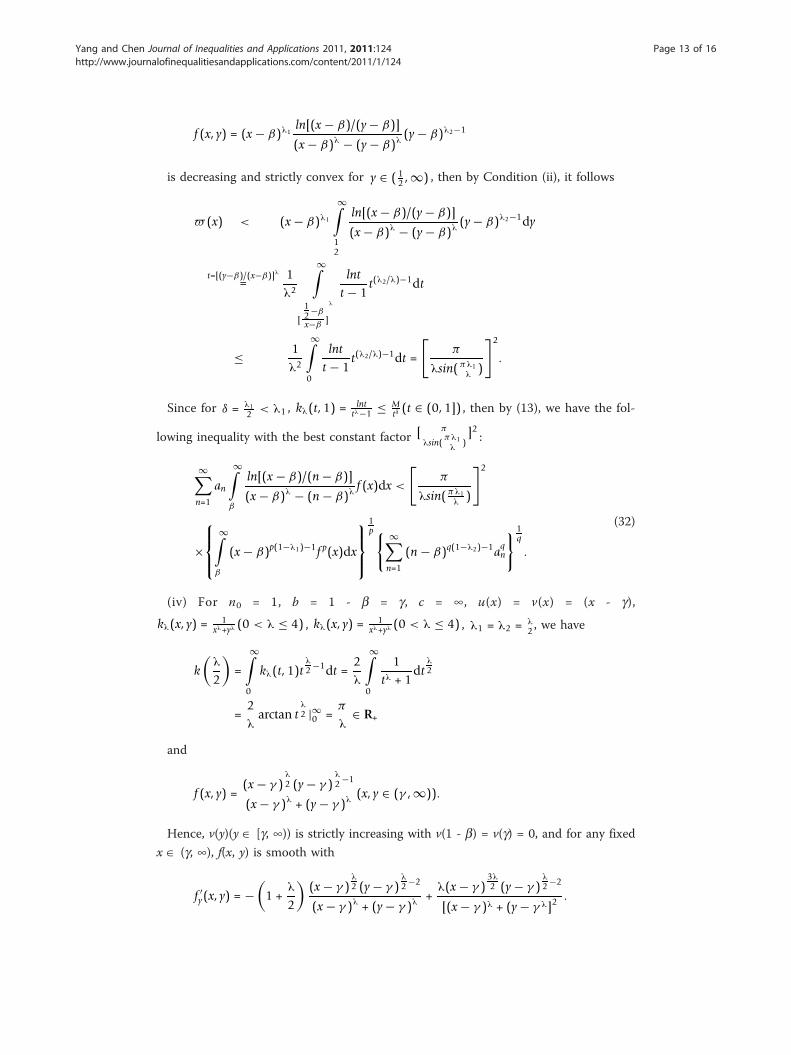
f (x, y) = (x − β)λ1ln[(x − β)/(y − β)]
(x − β)λ − (y − β)λ(y − β)λ2−1
is decreasing and strictly convex for y ∈ ( 12 ,∞) , then by Condition (ii), it follows
(x) < (x − β)λ1
∞∫12
ln[(x − β)/(y − β)]
(x − β)λ − (y − β)λ(y − β)λ2−1dy
t=[(y−β)/(x−β)]λ=
1λ2
∞∫
[
12−β
x−β]
λ
lntt − 1
t(λ2/λ)−1dt
≤ 1λ2
∞∫0
lnt
t − 1t(λ2/λ)−1dt =
[π
λsin(πλ1λ)
]2
.
Since for δ = λ12 < λ1 , kλ(t, 1) = lnt
tλ−1 ≤ Mtδ (t ∈ (0, 1]) , then by (13), we have the fol-
lowing inequality with the best constant factor [ π
λsin(πλ1λ
)]2 :
∞∑n=1
an
∞∫β
ln[(x − β)/(n− β)]
(x − β)λ − (n − β)λf (x)dx <
[π
λsin(πλ1λ)
]2
×
⎧⎪⎨⎪⎩
∞∫β
(x − β)p(1−λ1)−1f p(x)dx
⎫⎪⎬⎪⎭
1p { ∞∑
n=1
(n − β)q(1−λ2)−1aqn
} 1q
.
(32)
(iv) For n0 = 1, b = 1 - b = g, c = ∞, u(x) = v(x) = (x - g),
kλ(x, y) = 1xλ+yλ (0 < λ ≤ 4) , kλ(x, y) = 1
xλ+yλ (0 < λ ≤ 4) , λ1 = λ2 = λ2 , we have
k(
λ
2
)=
∞∫0
kλ(t, 1)tλ2−1dt =
2λ
∞∫0
1tλ + 1
dtλ2
=2λarctan t
λ2 |∞0 =
π
λ∈ R+
and
f (x, y) =(x − γ )
λ2 (y − γ )
λ2−1
(x − γ )λ + (y − γ )λ(x, y ∈ (γ ,∞)).
Hence, v(y)(y Î [g, ∞)) is strictly increasing with v(1 - b) = v(g) = 0, and for any fixed
x Î (g, ∞), f(x, y) is smooth with
f ′y(x, y) = −
(1 +
λ
2
)(x − γ )
λ2 (y − γ )
λ2−2
(x − γ )λ + (y − γ )λ+
λ(x − γ )3λ2 (y − γ )
λ2−2
[(x − γ )λ + (y − γ λ]2.
Yang and Chen Journal of Inequalities and Applications 2011, 2011:124http://www.journalofinequalitiesandapplications.com/content/2011/1/124
Page 13 of 16
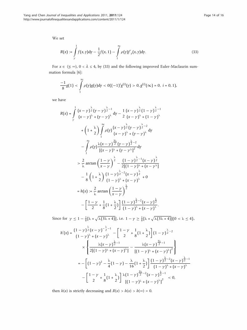
We set
R(x) :=
1∫γ
f (x, y)dy − 12f (x, 1) −
∞∫1
ρ(y)f ′y(x, y)dy. (33)
For x Î (g, ∞), 0 < l ≤ 4, by (33) and the following improved Euler-Maclaurin sum-
mation formula [6]:
−18
g(1) <
∞∫1
ρ(y)g(y)dy < 0((−1)ig(i)(y) > 0, g(i)(∞) = 0, i = 0, 1),
we have
R(x) =
1∫γ
(x − γ )λ2 (y − γ )
λ2−1
(x − γ )λ + (y − γ )λdy − 1
2(x − γ )
λ2 (1 − γ )
λ2−1
(x − γ )λ + (1 − γ )λ
+(1 +
λ
2
) ∞∫1
ρ(y)(x − γ )
λ2 (y − γ )
λ2−2
(x − γ )λ + (y − γ )λdy
−∞∫1
ρ(y)λ(x − γ )
3λ2 (y − γ )
λ2−2
[(x − γ )λ + (y − γ λ]2dy
>2λarctan
(1 − γ
x − γ
)λ2 − (1 − γ )
λ2−1(x − γ )
λ2
2[(1 − γ )λ + (x − γ λ]
− 18
(1 +
λ
2
)(1 − γ )
λ2−2(x − γ )
λ2
(1 − γ )λ + (x − γ )λ+ 0
= h(x) :=2λarctan
(1 − γ
x − γ
)λ2
−[1 − γ
2+18(1 +
λ
2)](1 − γ )
λ2−2(x − γ )
λ2
(1 − γ )λ + (x − γ )λ.
Since for γ ≤ 1 − 18 [λ +
√λ(3λ + 4)] , i.e. 1 − γ ≥ 1
8 [λ +√
λ(3λ + 4)](0 < λ ≤ 4),
h′(x) =(1 − γ )
λ2 (x − γ )−
λ2−1
(1 − γ )λ + (x − γ )λ−
[1 − γ
2+18(1 +
λ
2)](1 − γ )
λ2−2
×⎧⎨⎩ λ(x − γ )
λ2−1
2[(1 − γ )λ + (x − γ )λ]− λ(x − γ )
3λ2 −1
[(1 − γ )λ + (x − γ )λ]2
⎫⎬⎭
= −[(1 − γ )2 − λ
4(1 − γ ) − λ
16(1 +
λ
2)](1 − γ )
λ2−2(x − γ )
λ2−1
(1 − γ )λ + (x − γ )λ
−[1 − γ
2+18(1 +
λ
2)]
λ(1 − γ )3λ2 −2(x − γ )
λ2−1
[(1 − γ )λ + (x − γ )λ]2 < 0,
then h(x) is strictly decreasing and R(x) > h(x) > h(∞) = 0.
Yang and Chen Journal of Inequalities and Applications 2011, 2011:124http://www.journalofinequalitiesandapplications.com/content/2011/1/124
Page 14 of 16
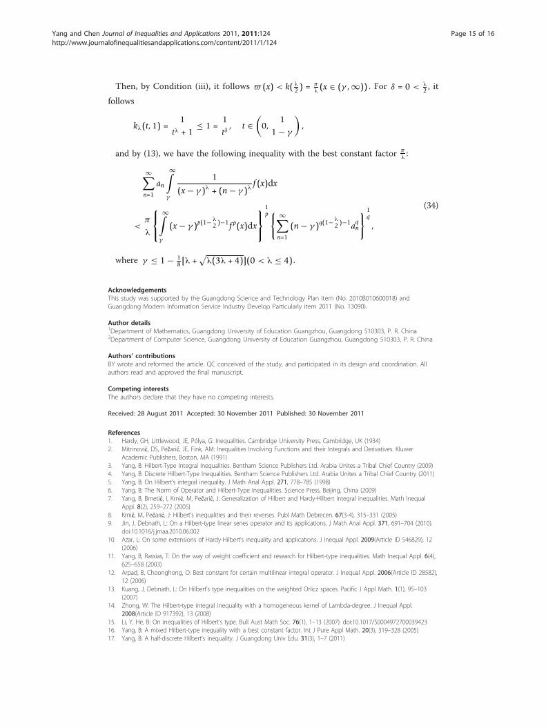
Then, by Condition (iii), it follows (x) < k(λ2 ) =
πλ(x ∈ (γ ,∞)) . For δ = 0 < λ
2 , it
follows
kλ(t, 1) =1
tλ + 1≤ 1 =
1tδ, t ∈
(0,
11 − γ
),
and by (13), we have the following inequality with the best constant factor πλ :
∞∑n=1
an
∞∫γ
1
(x − γ )λ + (n − γ )λf (x)dx
<π
λ
⎧⎨⎩
∞∫γ
(x − γ )p(1−λ2 )−1f p(x)dx
⎫⎬⎭
1p { ∞∑
n=1
(n − γ )q(1−λ2 )−1aqn
} 1q
,
(34)
where γ ≤ 1 − 18 [λ +
√λ(3λ + 4)](0 < λ ≤ 4) .
AcknowledgementsThis study was supported by the Guangdong Science and Technology Plan Item (No. 2010B010600018) andGuangdong Modern Information Service Industry Develop Particularly item 2011 (No. 13090).
Author details1Department of Mathematics, Guangdong University of Education Guangzhou, Guangdong 510303, P. R. China2Department of Computer Science, Guangdong University of Education Guangzhou, Guangdong 510303, P. R. China
Authors’ contributionsBY wrote and reformed the article. QC conceived of the study, and participated in its design and coordination. Allauthors read and approved the final manuscript.
Competing interestsThe authors declare that they have no competing interests.
Received: 28 August 2011 Accepted: 30 November 2011 Published: 30 November 2011
References1. Hardy, GH, Littlewood, JE, Pólya, G: Inequalities. Cambridge University Press, Cambridge, UK (1934)2. Mitrinović, DS, Pečarić, JE, Fink, AM: Inequalities Involving Functions and their Integrals and Derivatives. Kluwer
Academic Publishers, Boston, MA (1991)3. Yang, B: Hilbert-Type Integral Inequalities. Bentham Science Publishers Ltd. Arabia Unites a Tribal Chief Country (2009)4. Yang, B: Discrete Hilbert-Type Inequalities. Bentham Science Publishers Ltd. Arabia Unites a Tribal Chief Country (2011)5. Yang, B: On Hilbert’s integral inequality. J Math Anal Appl. 271, 778–785 (1998)6. Yang, B: The Norm of Operator and Hilbert-Type Inequalities. Science Press, Beijing, China (2009)7. Yang, B, Brnetić, I, Krnić, M, Pečarić, J: Generalization of Hilbert and Hardy-Hilbert integral inequalities. Math Inequal
Appl. 8(2), 259–272 (2005)8. Krnić, M, Pečarić, J: Hilbert’s inequalities and their reverses. Publ Math Debrecen. 67(3-4), 315–331 (2005)9. Jin, J, Debnath, L: On a Hilbert-type linear series operator and its applications. J Math Anal Appl. 371, 691–704 (2010).
doi:10.1016/j.jmaa.2010.06.00210. Azar, L: On some extensions of Hardy-Hilbert’s inequality and applications. J Inequal Appl. 2009(Article ID 546829), 12
(2006)11. Yang, B, Rassias, T: On the way of weight coefficient and research for Hilbert-type inequalities. Math Inequal Appl. 6(4),
625–658 (2003)12. Arpad, B, Choonghong, O: Best constant for certain multilinear integral operator. J Inequal Appl. 2006(Article ID 28582),
12 (2006)13. Kuang, J, Debnath, L: On Hilbert’s type inequalities on the weighted Orlicz spaces. Pacific J Appl Math. 1(1), 95–103
(2007)14. Zhong, W: The Hilbert-type integral inequality with a homogeneous kernel of Lambda-degree. J Inequal Appl.
2008(Article ID 917392), 13 (2008)15. Li, Y, He, B: On inequalities of Hilbert’s type. Bull Aust Math Soc. 76(1), 1–13 (2007). doi:10.1017/S000497270003942316. Yang, B: A mixed Hilbert-type inequality with a best constant factor. Int J Pure Appl Math. 20(3), 319–328 (2005)17. Yang, B: A half-discrete Hilbert’s inequality. J Guangdong Univ Edu. 31(3), 1–7 (2011)
Yang and Chen Journal of Inequalities and Applications 2011, 2011:124http://www.journalofinequalitiesandapplications.com/content/2011/1/124
Page 15 of 16

18. Kuang, J: Applied Inequalities. Shangdong Science Technic Press, Jinan, China (2004)19. Kuang, J: Introduction to Real Analysis. Hunan Education Press, Chan-sha, China (1996)
doi:10.1186/1029-242X-2011-124Cite this article as: Yang and Chen: A half-discrete Hilbert-type inequality with a homogeneous kernel and anextension. Journal of Inequalities and Applications 2011 2011:124.
Submit your manuscript to a journal and benefi t from:
7 Convenient online submission
7 Rigorous peer review
7 Immediate publication on acceptance
7 Open access: articles freely available online
7 High visibility within the fi eld
7 Retaining the copyright to your article
Submit your next manuscript at 7 springeropen.com
Yang and Chen Journal of Inequalities and Applications 2011, 2011:124http://www.journalofinequalitiesandapplications.com/content/2011/1/124
Page 16 of 16


