Abstract—This paper investigates residual vibrations of
industrial SCARA robots in wafer handling applications. Due
to rapid point-to-point movements, SCARA robot arms exhibit
large vibrations after reaching the destination position. A
mathematical model particularly suitable for residual vibration
analysis is developed. The validity of the mathematical model is
confirmed by the close match between experimental results and
robot arm trajectories generated by the model. The root cause
of residual vibrations is analyzed using the model. Based on the
root cause analysis, a practical solution to suppress vibrations is
proposed. The solution utilizes an acceleration smoother to
smooth the commanded trajectory, and it can be easily
implemented in practice without redesign the robot hardware
or control system. Experimental results show over 40%
reduction in both vibration amplitude and settling time.
Index terms—Industrial robot, Vibration, Modeling, Control.
1 INTRODUCTION
he robots studied in this paper refer to industrial SCARA
(Selectively Compliant Articulated Robot Arm) robots
for wafer handling as show in Fig. 1. Rapid point-to-point
movements for the robot arms are usually involved in
manufacturing environments. To transfer a wafer from one
point to another, the robot arm needs to go through a series
of motions involving accelerating to a required operational
speed and decelerating to a full stop. The abrupt changes in
acceleration or deceleration often result in residual
vibrations. Figure 1 shows a laser recorded vibration plot
(scale: 0.4mm/div) at robot’s end-effector after the arm
reachs the destination. The vibration may cause wafer
slippery and lead to long system settling time.
Fig. 1. A SCARA industrial robot and residual vibration.
To improve quality and efficiency of the manufacturing
WeiMin Tao is with Brooks Automation Inc. USA (e-mail:
[email protected]); MingJun Zhang is with Agilent Technologies, Plao
Alto, USA (e-mail: [email protected]); Ou Ma is with New Mexico
State University, USA (e-mail: [email protected]); XiaoPing Yun is with
Naval Postgraduate School, Monterey, USA (e-mail: [email protected]).
process, it is desired to understand the dynamics involved in
the process and to develop efficient methods to suppress the
vibration. The first thing is to identify the root cause of the
vibration by creating and studying its dynamics model.
Unfortunately, no well-developed models for studying the
residual vibration of such robot arms are available in the
open literature. The existing techniques of modeling SCARA
robots are mainly for motion control as opposed to vibration
control. In this paper, a dynamic model for vibration study of
this type of industrial robots is first presented. Based on the
dynamics model, a solution is then proposed to suppress the
vibration. The dedicated modeling provides a good reference
for similar industrial robots. The generic solution for
vibration suppression can also be applied to other industrial
applications.
The robot arm discussed here is driven by DC motors with
high gear ratios for power transmission. The end-effector in
the robot arm is connected to the motor through a number of
pulleys. The pulleys are connected through timing belts. One
advantage of this type of indirect drive system is its
variation-isolation effect since the inertial changes on the
payload have little effect on the actuator due to high
reduction ratio. Besides backlash and additional friction in
the transmission system, another disadvantage of the indirect
drive system is that the lumped elasticity of the transmission
system makes the robot arm work like a flexible manipulator
and isolates the direct motor control and position feedback
from the robot’s end-effector. The residual vibration
resulting from the elasticity (translation or rotation spring
impact of the timing belt) of the transmission system
sometimes becomes quite significant in a high-speed point-
to-point motion. There are a couple of existing approaches to
reduce or eliminate the vibration of a flexible structure:
• Increase damping by structural design or adding
dampers: to ensure big damping, high natural
frequency and stiffness [1][2];
• Open loop approaches: including trajectory
smoothing input shaping and feed-forward
approaches. The typical trajectory smoothing
approaches (also called S-curve motion profiling)
employ a multi order polynomial in time for trajectory
generation [3][4]. Trajectory smoothing reduces the
residual vibration by providing a smooth
acceleration/deceleration and accounting for motor
amplifier’s electrical saturation feature. Input shaping
approach convolves a sequence of impulses to
produce a shaped input as the motion command. It
reduces residual vibration by generating an input that
cancels its own vibration [5][6][7][8]. Feed-forward
Residual Vibration Analysis and Suppression for SCARA Robots in
Semiconductor Manufacturing
WeiMin TAO, MingJun ZHANG, Ou MA and XiaoPing YUN
T
End-effector Robot arm
INTERNATIONAL JOURNAL OF INTELLIGENT CONTROL AND SYSTEMSVOL. 11, NO. 2, JUNE 2006, 97-105
approaches typically make use of input and model
information to generate control output and to make
the plant follow the predefined vibration free
trajectory [9][1]. The open-loop approaches have to
work with close-loop control to achieve other control
objectives such as steady-state accuracy, system
stability and robustness against disturbances and
uncertainties.
• Close-loop approaches, such as conventional PID
control, adaptive PID control, model based adaptive
control [10][11][12][13], and H ∞ control design [14].
Due to the position difference of the end point (e.g.
end-effector) and the controlled point (e.g. robot
joint) of a flexible structure, the traditional collocated
control often failed to achieve satisfactory
performance. Non-collocated control approaches have
been proven to have better control performance
including vibration suppression [15][16][17].
However, this kind of approaches require additional
sensors at the end point.
The trajectory smoothing approach is one of the most
popular approaches currently used in industry. This is mainly
due to its simplicity, flexibility and universality. PID
feedback control is a primitive and robust robot control
approach, which is easy to implement and can provide
satisfactory control performance for varied dynamic
characteristics. Other approaches may require accurate
models, additional sensors, and/or intensive computations.
In this paper, the PID control and a generic motion profile
(S-curve) are applied to the robots to meet the general
requirements. The reason for selecting PID control approach
is its robustness and simplicity. The reason for selecting the
S-curve trajectory smoothing approach is, in addition to
other benefits mentioned above, that the PID approach is
incapable of keeping the system in critically damped
condition, which is important to eliminate or reduce the
vibration. This incapability is mainly due to implementation
constraints (tracking error limit, electrical noise etc). The
selected control scheme is able to meet most application’s
requirements. However, for some applications, which require
very smooth motion with very high speed, the existing
motion profile and control parameters fail to provide
acceptable performance. The goal of this study is to resolve
such an industrial problem by analyzing the root cause of the
vibration problem and providing a practical and robust
solution to the problem. For root-cause analysis, a dedicated
dynamics model of the SCARA arm set is created. The root
cause of arm vibration after motion completion is analyzed
based on this model. The modeling of the arm set mainly
takes into account factors of belt spring impact and damping
friction. Lagrange formulation is applied for modeling the
dynamics. A practical solution to reduce the residual
vibration is proposed and evaluated.
The rest of the paper is organized as follows. Section 2
provides the modeling of the inherent dynamics of the robot
arm with its parameters determined in section 3 using direct
measurement and system identification. Section 4 conducts
the root cause analysis of the vibration. Section 5 proposes a
practical solution to suppress the residual vibration. The test
results with two robots are presented in Section 6. Section 7
concludes the paper.
2 MODELING OF THE ROBOT ARM
2.1 SCARA Arm Robots
The modeling of the arm set in this work is mainly for
vibration analysis instead of for motion control. Some
assumptions in the modeling are made solely for the residual
vibration analysis.
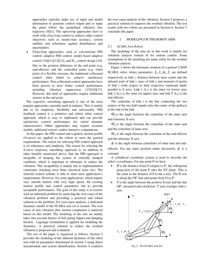
Figure 2 shows the kinematic notation of a general 3-DOF
SCARA robot, where parameters iiii ImlL ,,, are defined
respectively as link i, distance between mass center and the
inboard joint of link i, mass of link i, and moment of inertia
of link i (with respect to their respective rotational shafts
parallel to Z axis). Link 1 (L1) is the inner (or lower) arm;
link 2 (L2) is the outer (or upper) arm; and link T (Lt) is the
end-effector.
The centerline of link i is the line connecting the two
centers of the two half rounds (also the center of the pulleys)
at the end of the link.
1Θ is the angle between the centerline of the inner arm
and reference X-axis.
2Θ is the angle between the centerline of the outer arm
and the centerline of inner arm.
TΘ is the angle between the centerline of the end-effector
and the reference X-axis.
φ is the angle between centerlines of outer arm and end-
effector. For any static position under discussion, φ is a
constant.
A cylindrical coordinate system is used to describe the
robot’s coordinates. For any point P we have:
• R is the distance from O (origin) to P', the orthogonal
projection of the point P onto the XY plane. This is
the same as the distance of P to the z-axis. The R axis
is along the OP’ line and points from O to P’. • T is the angle between the positive X-axis and the line
OP', measured anti-clockwise. T axis overlaps with z-
axis.
Θ1
Θ2
Θt
L1
l1m
1I
1
L2
l2m
2I
2
Lt
ltm
t
Xo
I t
YR
T (z)
P(P?
Fig. 2. The SCARA Arm Set.
Tao et al.: Residual Vibration Analysis and Suppression for SCARA Robots in Semiconductor Manufacturing 98

• Z is the same as z.
The rotations of inner arm and outer arm are coupled by
the belt-driving system such that the centerline of the end-
effector axis always passes through the origin point O. So we
define R axis as the radial axis from O to the centerline of
the end-effector. The end-effector can only move along the
R, T and Z axes. TΘ is actually the rotational angle of end-
effector around T axis, which is determined by the rotation
of robot column bound with one end of the inner arm.
The residual vibration occurs after the arm reaches the
destination position. In order to investigate the motion of the
tip of end-effector after that, we make the following
assumptions:
• The motion of the tip of end-effector to be
investigated starts after the arm reaches the
destination, which means the reference time of
interest starts at the moment when the arm reaches the
destination.
• The active torque from the motor and static friction
approximately equal to zero after the arm reaches the
destination.
• After the arm reaches the destination, the robot
column and the inner arm that is connected to the
column, completely stop moving.
Since the inner arm is not moving after the arm reaches
the destination, the motion of the tip of end-effector is purely
the combined motion of the outer arm and end-effector. The
outer arm is connected through the belt B1 (located in inner
arm) to the column; while the end-effector is connected
through the belt B2 (located in outer arm) to the pulley,
which is connected to the inner arm as shown in Fig. 3.
The T motor is connected to the robot column and R
motor is connected to link 1. Both motors drive the T/R axes
through a number of timing belts with a big gear ratio. T
rotation drives both the robot column and link 1. R rotation
causes rotations in link 1, link 2 and link T through B1 and
B2 to ensure that the centerline of link T always passes
through the origin O. Apparently the motors do not directly
control the end-effector.
We assume that both the column and inner arm that is
bound to the column have completely stopped after the arm
reaches the destination. Then L1 is motionless and the
motions of L2 and the tip of the end-effector are restricted by
B1 and B2 due to their spring impact.
Fig. 3. Outer arm and end-effector connected by B1 and B2.
Two generalized coordinates are chosen to represent the
vibration from robot’s static pose:
• 1q = 2θ : The angle between the centerline of outer arm
and its static position (corresponding to the given T/R
destination position). This is the vibration angle
resulting from the rotational stiffness of B1.
• 2q =tθ : The angle between the centerline of the end-
effector and its static position with respect to L2
(corresponding to the given T/R destination position),
which maintains the same φ for any 2θ . This is the
vibration angle resulting from the rotational stiffness of
B2.
Figure 4 shows the geometric relationship between the arm’s
final static position (S) and dynamic vibration position (D).
Both arms’ positions are shown by the solid centerlines of
L1, L2 and Lt. Assuming the arm’s static position for the
given T/R destination position is:
=Θ
=Θ
=Θ
tts
s
s
α
α
α
22
11
where tααα ,, 21 are constant angles. For any dynamic
vibration position, we have:
222 αθ −Θ= and 2θαθ −−Θ= ttt
tαααφ −+= 21
The angular velocities are •
2θ and •
tθ
2.2 Lagrange’s Equations
It can be seen that B1 and B2 are not inter-connected;
hence their motion due to belts’ elongation is independent.
However, since end-effector is mounted on L2, the motion of
the tip of end-effector results from the combined motion of
both L2 and Lt.
The kinetic energy of L2 and Lt is as follows:
2
2
22
22
2
22 )(2
1
2
1
2
1
2
1 •••
++++= tttctc IVmIVmK θθθ (1)
Fig. 4. Geometric relationship of the static and dynamic positions.
1α
2α
tα
φφ
φ
2θ
2θ
tθ2θ
tθφ −
2V
2V
2tV
S
DY
x1L
tL
2L2L
tL
L1
I
L2
Lt
X
YR
B1
B2
lt
l2
Robot Column
End-effector
Shaft linked to L199
99 INTERNATIONAL JOURNAL OF INTELLIGENT CONTROL AND SYSTEMS, VOL. 11, NO. 2, JUNE 2006
where I2 and It are the moments of inertia with respect to the
axes passing through the mass centers of L2 and Lt,
respectively. V2c and Vtc are the respective velocities of the
mass centers of L2 and Lt.
Assume that the mass centers of L2 and Lt are along their
respective axis (symmetric mass distribution) and their
distances to the center of rotation shaft are l2 and lt (shown in
Fig. 3). The velocity of mass centers of L2 and Lt can be
computed based on the geometric relationship of L2 and Lt
shown in Fig. 4. Vtc is the sum of V2 (= 32 l•
θ , the velocity at
the rotation shaft of Lt) and Vt2 (= tt l•
θ , the relative velocity
of Lt with respect to L2). We then have: •
= 222 θlV c ;
)cos(2)()( 32
22
32
2ttttttc llllV θφθθθθ −−+=
••••
where l3 is the distance between the center of the rotation
shaft of Lt and the center of rotation shaft of L2. Generally,
we have tθφ >> (the vibration angle is relatively small in
most discussed arm positions). Thus,
φθφ cos)cos( ≈− t .
The potential energy of L2 and Lt is mainly from the two
belts B1/B2:
2
2
2
212
1
2
1tkkP θθ += (2)
where 1k and 2k are respectively the rotational stiffness of
B1 and B2.
The Lagrangian becomes
PKL −=
The Rayleigh Dissipation (R) function is:
2
2
2
212
1
2
1 ••
+= tccR θθ (3)
where 1c and 2c are the lump sum damping coefficients of
L2 and Lt respectively.
The Lagrange’s equation can be written as:
i
iii
Mq
L
q
R
q
L
dt
d=
∂
∂−
∂
∂+
∂
∂••
)( for i=1 and 2. (4)
where, Mi (for i=1, 2) are the torques applied to L2 and Lt
respectively. M1 includes motor torque Mm and static friction
torque. M2 is only static friction torque. Applying (1)-(3) to
the Lagrange’s equation in (4), we have:
=++−
++
=++−
++++
•••
••
•••
••
22223
2
121213
2
2
32
2
22
)cos(
)(
)cos(
)(
MkcllmI
Ilm
MkcllmI
lmIIlm
ttttt
tttt
tttt
tt
θθθφ
θ
θθθφ
θ
(5)
It is noted that φ is constant for a given destination
position. As a result, Eq. (5) represents a two-input two-
output linear system.
3 PARAMETER DETERMINATION
3.1 Measurement and Experiment
Through measurements and experimental tests, we have
obtained the following parameters show in table 1.
Table 1. Physical Parameters of A SCARA Robot
m2 0.533 kg
mt 0.533 kg
l2 0.115 m
lt 0.095 m
I2 0.0035 (kg.m2)
It 0.00137 kg.m2
l3 0.19 m
In (5), 1c , 2c 1k , and 2k are unknown parameters.
Though translational spring constants of B1/B2 can be
obtained through experiment, it’s still a challenge to compute
the rotational stiffness due to the difficulty in determining the
tooth stiffness. In order to identify the above unknown
parameters, we use system identification approach to
compute them based on testing data.
3.2 System identification
MatLab System Identification programs are developed to
calculate the four unknown parameters. First, we write the
Eq. (5) in a state space form. We define the following state
variables:
tt xxxx θθθθ ====••
423221 ;;;
The state space equation is :
+=
+=•
DUCXY
BUAXX (6)
where, TxxxxX ][ 4321= and
TxxY ][ 43=
To investigate the motion after the arm reaches the
destination, we assume that the active torque from motor and
static friction are negligible (measurement of motor current
verified this) and the end-effector motion is purely
dominated by the initial condition of X, spring impact of
B1/B2 (rotational stiffness), viscous friction, and the inertial
of L2 and Lt. In this case, U in Eq. (6) is zero.
The actual output data Y ( 2θ and tθ ) are computed from
recorded laser data 2θ and tθθ +2 . The output data and the
initial values of X are applied to Eq. (6) by the system
identification program, and the unknown parameters of A in
equation (6) are identified using PEM function in MATLAB
(The function PEM provides an unbiased estimation
method), and then the unknown parameters 1c , 2c , 1k and
2k are obtained. Below is a set of identified parameters for
one of the robots:
1c =0.293; 2c =0.1; 1k =439; 2k =167.5
After parameter estimation, the model outputs are
Tao et al.: Residual Vibration Analysis and Suppression for SCARA Robots in Semiconductor Manufacturing 100
compared with the actual output data to verify the system
identification results. Both back validation and cross
validation are performed. Back validation compares the
model output with the actual output driven by the data used
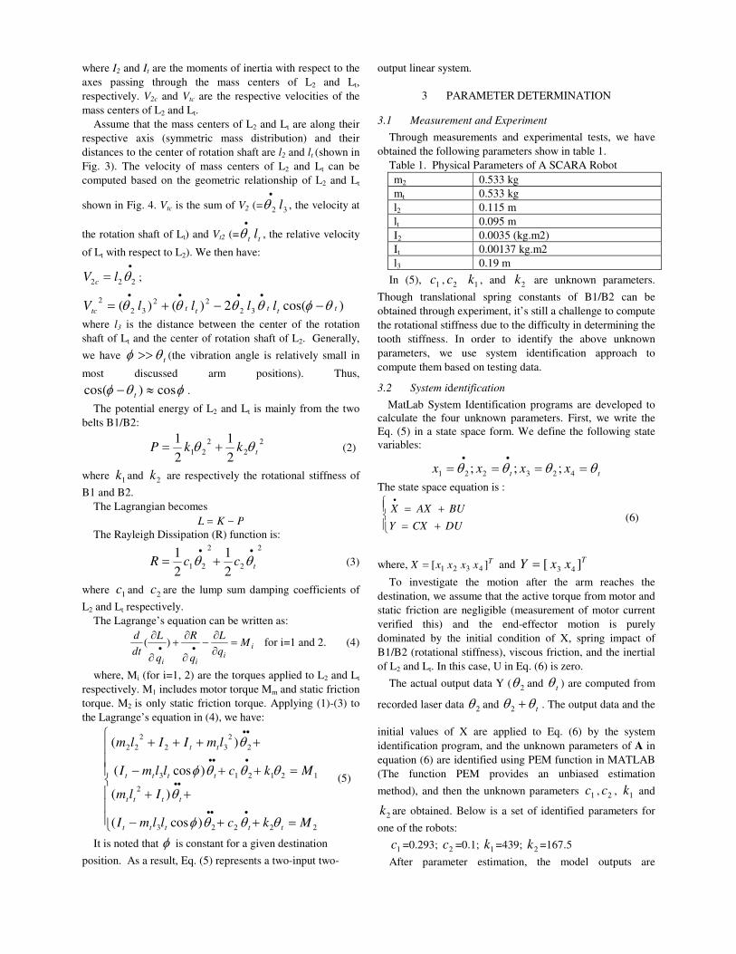
for system identification. Figure 5 shows the back validation
of end-effector vibration. The Y-axis is the output of
tθθ +2 in radian; X-axis is the time in second. The black
plot is real test data; the grey plot is the model output.
The back validation shows fairly good matching between
the model output and the actual output.
Fig. 5. Back validation of end-effector vibration.
The cross validation is also conducted for model
verification. Cross validation compares the model output
with the actual output driven by the data not used for system
identification. The cross validation results also show a good
match between model output and actual output except for the
cases with small vibration amplitude. The main reason could
be that with small vibration amplitude other factors which
are not taken into account in the arm modeling become
dominant, e.g., the small vibration resulting from the belts
which connects T/R motors to robot column and L1, static
friction and non-linearity factors.
4 ROOT CAUSE ANALYSIS
4.1 Output Analysis
Intuitively we can see that the rotational spring impact of
the timing belts plays a major rule in converting the potential
energy to the kinetic energy and vice versa, which causes the
residual vibration at the end-effector. This perception can be
explored by investigating the transfer function of the output
2θ and tθ to the motor torque input Mm, which can be
expressed as follows:
=)(/)(2 sMs mθ
1275000000169500015710016.16
105802.423008892.000289.0234
23
++++
−+−
SSSS
SSS
=)(/)( sMs mtθ
1275000000169500015710016.16
32684.16305101.000105.0234
23
++++
−+−
SSSS
SSS
After the robot arm reaches the destination, the motor
torque and the static friction torque are considered as zero.
The outputs 2θ and tθ depend mainly on their initial
condition and poles of their transfer function. The
denominator polynomial of the transfer function is of the
forth order. Its coefficients are functions of the spring
rotational stiffness of B1 and B2, viscous damping
coefficients and the inertial of L2 and Lt. These coefficients
determine the poles’ location of the denominator polynomial.
The vibration characteristics are also determined by those
factors.
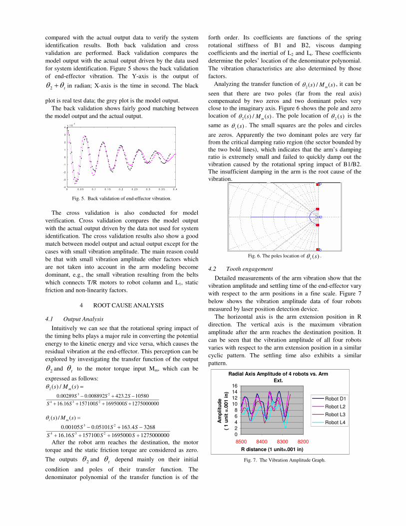
Analyzing the transfer function of )(/)(2 sMs mθ , it can be
seen that there are two poles (far from the real axis)
compensated by two zeros and two dominant poles very
close to the imaginary axis. Figure 6 shows the pole and zero
location of )(/)(2 sMs mθ . The pole location of )(2 sθ is the
same as )(stθ . The small squares are the poles and circles
are zeros. Apparently the two dominant poles are very far
from the critical damping ratio region (the sector bounded by
the two bold lines), which indicates that the arm’s damping
ratio is extremely small and failed to quickly damp out the
vibration caused by the rotational spring impact of B1/B2.
The insufficient damping in the arm is the root cause of the
vibration.
Fig. 6. The poles location of )(stθ .
4.2 Tooth engagement
Detailed measurements of the arm vibration show that the
vibration amplitude and settling time of the end-effector vary
with respect to the arm positions in a fine scale. Figure 7
below shows the vibration amplitude data of four robots
measured by laser position detection device.
The horizontal axis is the arm extension position in R
direction. The vertical axis is the maximum vibration
amplitude after the arm reaches the destination position. It
can be seen that the vibration amplitude of all four robots
varies with respect to the arm extension position in a similar
cyclic pattern. The settling time also exhibits a similar
pattern.
Radial Axis Amplitude of 4 robots vs. Arm
Ext.
0
2
4
6
8
10
12
14
16
8500 8400 8300 8200
R distance (1 unit=.001 in)
Am
pli
tud
e
( 1 u
nit
=.0
01 i
n)
Robot D1
Robot L2
Robot L3
Robot L4
Fig. 7. The Vibration Amplitude Graph.
0 0 .0 5 0 .1 0 .1 5 0 .2 0 .2 5 0 .3 0 .3 5 0 .4-4
-3
-2
-1
0
1
2
3
4x 1 0
- 3
101 INTERNATIONAL JOURNAL OF INTELLIGENT CONTROL AND SYSTEMS, VOL. 11, NO. 2, JUNE 2006
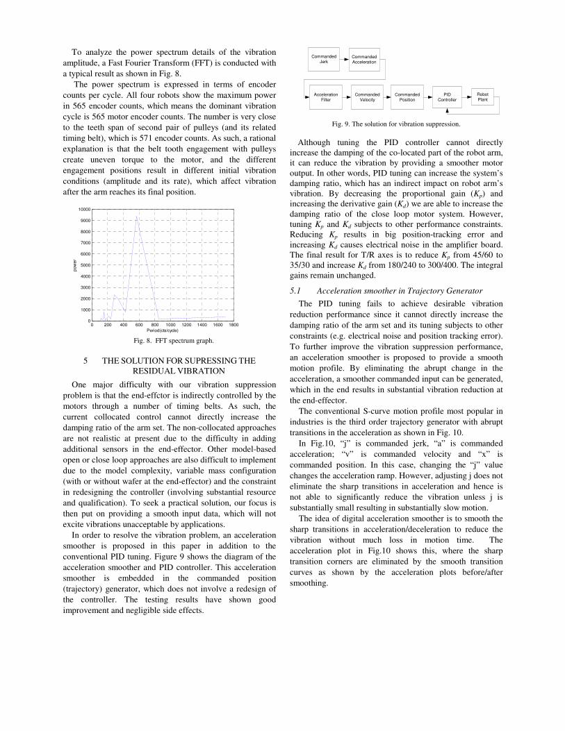
To analyze the power spectrum details of the vibration
amplitude, a Fast Fourier Transform (FFT) is conducted with
a typical result as shown in Fig. 8.
The power spectrum is expressed in terms of encoder
counts per cycle. All four robots show the maximum power
in 565 encoder counts, which means the dominant vibration
cycle is 565 motor encoder counts. The number is very close
to the teeth span of second pair of pulleys (and its related
timing belt), which is 571 encoder counts. As such, a rational
explanation is that the belt tooth engagement with pulleys
create uneven torque to the motor, and the different
engagement positions result in different initial vibration
conditions (amplitude and its rate), which affect vibration
after the arm reaches its final position.
Fig. 8. FFT spectrum graph.
5 THE SOLUTION FOR SUPRESSING THE
RESIDUAL VIBRATION
One major difficulty with our vibration suppression
problem is that the end-effctor is indirectly controlled by the
motors through a number of timing belts. As such, the
current collocated control cannot directly increase the
damping ratio of the arm set. The non-collocated approaches
are not realistic at present due to the difficulty in adding
additional sensors in the end-effector. Other model-based
open or close loop approaches are also difficult to implement
due to the model complexity, variable mass configuration
(with or without wafer at the end-effector) and the constraint
in redesigning the controller (involving substantial resource
and qualification). To seek a practical solution, our focus is
then put on providing a smooth input data, which will not
excite vibrations unacceptable by applications.
In order to resolve the vibration problem, an acceleration
smoother is proposed in this paper in addition to the
conventional PID tuning. Figure 9 shows the diagram of the
acceleration smoother and PID controller. This acceleration
smoother is embedded in the commanded position
(trajectory) generator, which does not involve a redesign of
the controller. The testing results have shown good
improvement and negligible side effects.
CommandedJerk
CommandedAcceleration
CommandedPosition
CommandedVelocity
AccelerationFilter
PIDController
RobotPlant
Fig. 9. The solution for vibration suppression.
Although tuning the PID controller cannot directly
increase the damping of the co-located part of the robot arm,
it can reduce the vibration by providing a smoother motor
output. In other words, PID tuning can increase the system’s
damping ratio, which has an indirect impact on robot arm’s
vibration. By decreasing the proportional gain (Kp) and
increasing the derivative gain (Kd) we are able to increase the
damping ratio of the close loop motor system. However,
tuning Kp and Kd subjects to other performance constraints.
Reducing Kp results in big position-tracking error and
increasing Kd causes electrical noise in the amplifier board.
The final result for T/R axes is to reduce Kp from 45/60 to
35/30 and increase Kd from 180/240 to 300/400. The integral
gains remain unchanged.
5.1 Acceleration smoother in Trajectory Generator
The PID tuning fails to achieve desirable vibration
reduction performance since it cannot directly increase the
damping ratio of the arm set and its tuning subjects to other
constraints (e.g. electrical noise and position tracking error).
To further improve the vibration suppression performance,
an acceleration smoother is proposed to provide a smooth
motion profile. By eliminating the abrupt change in the
acceleration, a smoother commanded input can be generated,
which in the end results in substantial vibration reduction at
the end-effector.
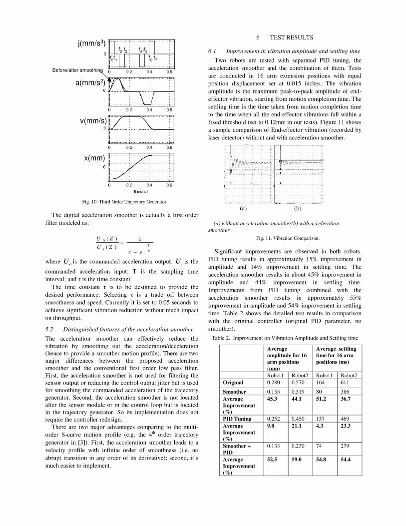
The conventional S-curve motion profile most popular in
industries is the third order trajectory generator with abrupt
transitions in the acceleration as shown in Fig. 10.
In Fig.10, “j” is commanded jerk, “a” is commanded
acceleration; “v” is commanded velocity and “x” is
commanded position. In this case, changing the “j” value
changes the acceleration ramp. However, adjusting j does not
eliminate the sharp transitions in acceleration and hence is
not able to significantly reduce the vibration unless j is
substantially small resulting in substantially slow motion.
The idea of digital acceleration smoother is to smooth the
sharp transitions in acceleration/deceleration to reduce the
vibration without much loss in motion time. The
acceleration plot in Fig.10 shows this, where the sharp
transition corners are eliminated by the smooth transition
curves as shown by the acceleration plots before/after
smoothing.
0 200 400 600 800 1000 1200 1400 1600 18000
1000
2000
3000
4000
5000
6000
7000
8000
9000
10000
po
we
r
Period(cts/cycle)
Tao et al.: Residual Vibration Analysis and Suppression for SCARA Robots in Semiconductor Manufacturing 102
x(mm)
v(mm/s)
a(mm/s2)
j(mm/s3)
Before/after smoothing
Fig. 10. Third Order Trajectory Generator.
The digital acceleration smoother is actually a first order
filter modeled as:
τ
Ti
ez
z
ZU
ZU
−
−
=)(
)(0
where oU is the commanded acceleration output; iU is the
commanded acceleration input; T is the sampling time
interval; and τ is the time constant.
The time constant τ is to be designed to provide the
desired performance. Selecting τ is a trade off between
smoothness and speed. Currently it is set to 0.05 seconds to
achieve significant vibration reduction without much impact
on throughput.
5.2 Distinguished features of the acceleration smoother
The acceleration smoother can effectively reduce the
vibration by smoothing out the acceleration/deceleration
(hence to provide a smoother motion profile). There are two
major differences between the proposed acceleration
smoother and the conventional first order low pass filter.
First, the acceleration smoother is not used for filtering the
sensor output or reducing the control output jitter but is used
for smoothing the commanded acceleration of the trajectory
generator. Second, the acceleration smoother is not located
after the sensor module or in the control loop but is located
in the trajectory generator. So its implementation does not
require the controller redesign.
There are two major advantages comparing to the multi-
order S-curve motion profile (e.g. the 4th
order trajectory
generator in [3]). First, the acceleration smoother leads to a
velocity profile with infinite order of smoothness (i.e. no
abrupt transition in any order of its derivative); second, it’s
much easier to implement.
6 TEST RESULTS
6.1 Improvement in vibration amplitude and settling time
Two robots are tested with separated PID tuning, the
acceleration smoother and the combination of them. Tests
are conducted in 16 arm extension positions with equal
position displacement set at 0.015 inches. The vibration
amplitude is the maximum peak-to-peak amplitude of end-
effector vibration, starting from motion completion time. The
settling time is the time taken from motion completion time
to the time when all the end-effector vibrations fall within a
fixed threshold (set to 0.12mm in our tests). Figure 11 shows
a sample comparison of End-effector vibration (recorded by
laser detector) without and with acceleration smoother.
(a) (b)
(a) without acceleration smoother(b) with acceleration
smoother
Fig. 11. Vibration Comparison.
Significant improvements are observed in both robots.
PID tuning results in approximately 15% improvement in
amplitude and 14% improvement in settling time. The
acceleration smoother results in about 45% improvement in
amplitude and 44% improvement in settling time.
Improvements from PID tuning combined with the
acceleration smoother results in approximately 55%
improvement in amplitude and 54% improvement in settling
time. Table 2 shows the detailed test results in comparison
with the original controller (original PID parameter, no
smoother).
Table 2. Improvement on Vibration Amplitude and Settling time
Average
amplitude for 16
arm positions
(mm)
Average settling
time for 16 arm
positions (ms)
Robot1 Robot2 Robot1 Robot2
Original 0.280 0.570 164 611
Smoother 0.153 0.319 80 386
Average
Improvement
(%)
45.3 44.1 51.2 36.7
PID Tuning 0.252 0.450 157 469
Average
Improvement
(%)
9.8 21.1 4.3 23.3
Smoother +
PID
0.133 0.230 74 279
Average
Improvement
(%)
52.5 59.0 54.8 54.4
(a)
(b)
103 INTERNATIONAL JOURNAL OF INTELLIGENT CONTROL AND SYSTEMS, VOL. 11, NO. 2, JUNE 2006