RIC 2010External Flood and Extreme PrecipitationExternal Flood and Extreme Precipitation Hazard Analysis for Nuclear Plant Safety
Recent Advances in Storm Surge ModelingDonald T ResioDonald T. Resio
US Army Engineer Research and Development Center11 March 2010
1

Outline
- Historical perspective.
- Getting a single storm right: The physics of single storm.
- Estimating the statistical likelihood of surges, including uncertaintyuncertainty.
- Estimating very-low-probability (annual frequency less
2
g y p y ( q ythan 10-6 annual probability) surge levels.

Design Storm Concept- Define a single storm that can be used to estimate design conditionsDefine a single storm that can be used to estimate design conditions.
Advantage – only have to model a single storm. BUT, this should be an objective definition if this storm is to be rigorously defined.
N d t d t i t t f E l t di h- Need to determine a storm surrogate for surge. Early studies chose storm intensity (wind speed) for this purpose – Saffir-Simpson Scale analogue – Standard Project Hurricane (SPH) and Maximum Probable Hurricane (PMH) were defined.
- Definitions were quite subjective, incorporating words such as “reasonably characteristic” and “expected to occur.”
- Data basis used in these early definitions and the models utilized in their execution were quite primitive.
3

GIWW on the morning that Katrina made landfall.
This storm exceeded both the SPH and PMH inmost areas in Southeast Louisiana and along theMississippi coast.
4

1st Step Model Storm Surge in Single Event1st Step Model Storm Surge in Single Event
Note that thesurge levelsstill increaseinland This
Accuracy of predictions critically dependent upon:
1) Resolution of the Physical System,
2) Accuracy of Hurricane Wind Fields,
inland. Thishas to beaccurately
d l d!!!
5
) y
3) Physics Captured Within Coupled Wave-Surge Model modeled!!!

Hurricane Surge Prediction
Wind Fields
Surge Models Wave Models
coupled
Overtopping + Loads on Structures
Local-scale waves
pp g
Surges outside and inside levee system
Response to Loads and Operational Considerations
Hazard Risk
6
Surges outside and inside levee systemHazard Risk
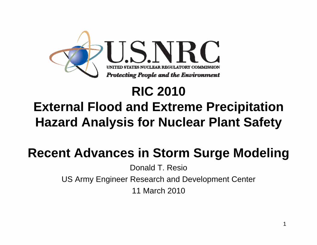
1Estimated relative contribution of waves to total surge
On steep slopes, waves become the dominant
alsu
rge
0 .8surge generator. This includes local scale near levees.
Examples: reefed islands and many rocky coastlines. About 30% of total surge during Hurricane Opal in Panama City
etup
toto
ta
0 .6Upper and lower limits of typicalwave model contributions to total
About 30% of total surge during Hurricane Opal in Panama City.
ofw
ave
se
0 .4
On very shallow slopes, wave set-
surge – not a universal constant -cannot be simply “factored out.”
ratio
o
0 .2
On very shallow slopes, wave setup is still important. Added about 2-4 feet of surge in Hurricane Katrina
71 /s lo p e
0 2 0 0 0 4 0 0 0 6 0 0 0 8 0 0 0 1 0 0 0 00

“Flooding can be a complexprocess – Flood protectionp pmust be addressed on asystems basis”L t ti l tLarge computational systemsoften trade off details forsystem compatibility “A model should be asA model should be as
simple as possible …but no simpler”
A. EinsteinExtreme events often transcend the empirical calibration basis of operational
d l d th i ht h i !
8
models = need the right physics!

Accuracy for a single event with IPET prediction system, including objective friction
ifi ti ith “b t” i dspecification with “best” winds
Figure 5: Comparison of observed USACE High Water Marks (HWM) for Hurricane Katrinaand the simulation using the H*WIND/IOKA wind fields. The red points are the values at therecorded USACE HWMs. Thin blue lines display a 1:1 correlation as well as 1.5 ft variance on
9
eco ded US C s b ue es d sp ay a co e at o as e as 5 t a a ce oeach side.

Accuracy for a single event with IPET prediction system, including objective friction
ifi ti ith t i i dspecification with parametric winds
Comparison of observed USACE HWMs for Hurricane Katrina and the simulation using thePBL wind fields. at the recorded USACE HWMs. Thin blue lines display a 1:1 correlation as wellas 1 5 ft variance on each side
10
as 1.5 ft variance on each side.

2nd Step Model Storm Surges Range of Events2nd Step Model Storm Surges Range of Events1970’s – Joint Probability Method
1990’s – Historical Storm Approach
Post-Katrina – Joint Probability Method – Optimal Sampling
11

Historical Statistical Approach
Katrina100 100010
Return period
Addition of 1 stormSeveral studies
Direct HitAsymptote
Katrina Addition of 1 storm creates a very largedeviation in the 100-yrsurge level. From over1000 years to about
have now shownthat the historicalstorm approachproduces very
1947Betsy
Rita
1000 years to about 100 years and if we useless years in our recordit could be the 65-yearstorm or less
produces veryunstable valuesfor extrapolatedreturn periods.A i l t
Non-Event Asymptote
storm or less.A single stormcan change theresults markedly. Location
Culprits:
• Storm size• Storm infrequency
12
• Storm infrequency

Statistical Approach – JPM with Optimal Sampling(JPM-OS)
G l f f t l ti d ti tmax 0( , ) ( , | , , , , , , ( ), )
where( , ) is the storm surge at location x and time t,
p fx t G W c R v B x S t t
x t
ζ θ
ζ
= Φ
General form for surge response at location x and time t:
( , ) is the storm surge at location x and time t, is a numerical model used to generate surges over a grid, is a time invariant grid of bathymetry/topogr
x t
G
ζΦ
aphy, is a wind field over the grid at time t,is the central pressure,
Wc
max
is the central pressure, is the radius to maximum wind speed from the center of the storm,
is the forward velocity of the storm, is the geograp
p
f
cRvθ hic angle of the track,
is the Holland "B" parameterB
0
is the Holland B parameter, is the landfall location, and
( ) is the position of the storm along the track at time t,
BxS t
Bottom line: There are 6 important storm parameters plus storm track and the
13
p p pchanges in near-coast storms that have to be considered in JPM.

Part of getting the winds right is capturing the near-coast variation in
Based on data fromO th d
p gstorm characteristics.
LAND WATER
Oceanweather, decayduring approach to land is about the sameas post-landfall decay.p y
Definition of values atlandfall gives a consistentmeasure of storm intensity!Average decay is 15 – 20 millibars over last 90 nm
14
millibars over last 90 nm.

Rmax increasesby about 30%over last 90 nm
Variation in Rmax
Also Holland Bdiminishes
Variation in Rmaxduring approach to land
Variation in Rmax as a function of position relative to landfall
15
Variation in Rmax as a function of position relative to landfall.

In any dimension we have for the pdf the ability to map froman n-dimensional space into a 1-dimensional space via aDirac delta-function δ
1 2 1 2 1( ) ( , ,..., ) [ ( , ,..., ) ] ...
is a parameter affecting hurricane surge levels
n n n
i
p p x x x x x x dx dx
x
η δ η= Ψ −∫∫∫p g g
(.) is the pdf is the surge level
i l ti l t ( d li t ) th t t
i
pηΨ is an analytical operator (modeling system) that coverts Ψ
i a specific set of values of x to a surge
And the CDF which uses the Heaviside Function (an integral of the delta function)
1 2 1 2 1 2( ) ... ( , ,..., ) [ ( , ,..., )] ...n n nF p x x x H x x x dx dx dxη η= − Ψ∫ ∫
And the CDF which uses the Heaviside Function (an integral of the delta function)
16

( ) ( ) [ ( ) ]F p x x x H x x x dx dx dx dη ε η ε ε= Ψ +∫ ∫
Since we remain imperfect, we need to consider an error term also!!!!
1 2 1 2 1 2( ) ... ( , ,..., , ) [ ( , ,..., ) ] ...
is the uncertainty in the surge level from the modelingn n nF p x x x H x x x dx dx dx dη ε η ε ε
ε
= − Ψ +∫ ∫
Thi th t l d f d i l tiThis means that we can leave some degree of randomness in our solutions – aslong as we can estimate the statistical characterization of this term – which alsoincludes tides, wind field errors, errors in physics, other omissions, etc.
The expected return period can be estimated from the CDF via the assumption thatthe storm occurrence is governed by a stationary Poisson process, with an averagefrequency of occurrence of λ.
11( )[1 ( )]
TF
ηλ η
=−
Unfortunately, nature often deviates from this simplistic assumptions – with years
17
containing many storms not following the same distribution as years with few storms

The hurricane population in the Gulf of Mexico appear to be mixed
960
980
Best F it G E V D istributionD ataBest F it G um bel D istribution 960
980
Best F it G E V D istributionD ataBest F it G um be l D istribution
Gulf of Mexico appear to be mixed.ra
lPre
ssur
e(m
b)
900
920
940
ralP
ress
ure
(mb)
900
920
940
Cen
t
10 0 10 1 10 2 10 3840
860
880 Cen
tr
10 0 10 1 10 2 10 3840
860
880
R eturn P eriod (years)
1r
nTm+
=
Figure 9c. Best-fit GEV and Gumbel distributions for GOM central pressures along with the data plotted with a simple
plotting position where n= number of years in the sample and m=rank for all storms in years with 4 or less storms occurring
R eturn P eriod (years)
plotting position, where n number of years in the sample and m rank, for all storms in years with 4 or less storms occurringin that year in left panel and all storms in years with more than 4 storms.
NOTE: Over a 30 mb difference (>5 ft surge for New Orleans area) at 100 year return period!
18

Statistical Approach – JPM with Optimal Sampling (JPM-OS)
( )R θ Λ Λ Λ Λ ΛJoint probability matrix:
2
1 2 3 4 5
0 1 01
1
( ( ) )
( , , , , )
[ ( ), ( )] ( )( | ) exp exp (Gumbel Distribution)( | ) ( )
p p f l
pp
R P R
p c R v x
F a x a x p a xp c xp c x a x
θ
Δ
= Λ ⋅ Λ ⋅ Λ ⋅ Λ ⋅ Λ
⎧ ⎫⎧ ⎫⎡ ⎤∂ ∂ Δ −⎪ ⎪Λ = = = − −⎨ ⎨ ⎬ ⎬⎢ ⎥∂ Δ ∂ ⎣ ⎦⎪ ⎪⎩ ⎭⎩ ⎭2
2( ( ) )
2 ( )2
( (
3
1( | )( ) 2
1( | )2
p p
f l
R P RP
p p
v
f l
p R c eP
p v e
σ
θ
σ π
θ
Δ −−
Δ
−
Λ = =Δ
Λ = =2
2) )
2fv
σ
− , , , , *(| | / 2)i j k l mp η η δ− <∑2f σ π
2
2( ( ) )
2 ( )4
1( | )( ) 2
l lxx
lp x ex
θ θσθ
σ π
−−
Λ = =
5 ( )xΛ = Φ
Different storms canproduce results in the
19
produce results in the same bin.

Summarizing:Uncertainty arises in all estimates due to lack of knowledge:
- Sample size effects- Lack of “science” effects
Sample Size Effects:- Sample size effects can be estimated based on coefficients of variation in the sample itself. - Samples with large coefficients of variations are indicative of more uncertainty in the estimated values for given return periods.- Typical 90% values in surge level uncertainty at the 100-year return
i d i th 2 4 f tperiod are in the range 2 – 4 feet
Lack of Science Effects:- Omissions of tides, deviations from parameterized wind fields, variations in near-coast rates of change, etc.- Errors in numerical models
The sum of of this uncertainty is added statistically to each estimated surge
20
y y gvalue befor it is included in the JPM computation

Probabilistic-Only Approach produces largeuncertainties in very-low probability surges
Uncertainty in an estimate is very difficult to estimate withoutsome assumption regarding the parent distribution and the“effective” number of samples (which depends on the spatial
y p y g
~ , where is the rms of the Gaussian uncertainty bandx xTS Sφ ⎛ ⎞
⎜ ⎟⎝ ⎠
autocorrelation attributes of the phenomenon). For extremes, thesetend to vary as a function of return period and number of samples.
Note:
2
, y
For a Gumbel Distribution, with a distributional rms of
1.100 1.1396 1~ for large ln( )
x xNS
y y TS S T y T
φ ⎜ ⎟⎝ ⎠
+ +≈ −
Note:Re-samplingdoes not includesample size dependence.
~ , for large ln( )2xS S T y T
N≈ −
nTTn
≈The “return period” of an eventshould be defined in a mannerwhich considers the design life
For largeT
Unfortunately, this makes the estimation of very-low- probabilityevents very uncertain – about the same magnitude as the surgelevel itself Is there a good alternative??
which considers the design life.
21
level itself. Is there a good alternative??

Characteristics & Form of Surge Response Functions (SRF)
1 2
3 4
75 simulations:Along coast variation and effect oft l t t ll d l
22
mean error = 0 – +4 cm, RMS error = 12 – 24 cmstorm angle at coast all produce clearmaximum values.
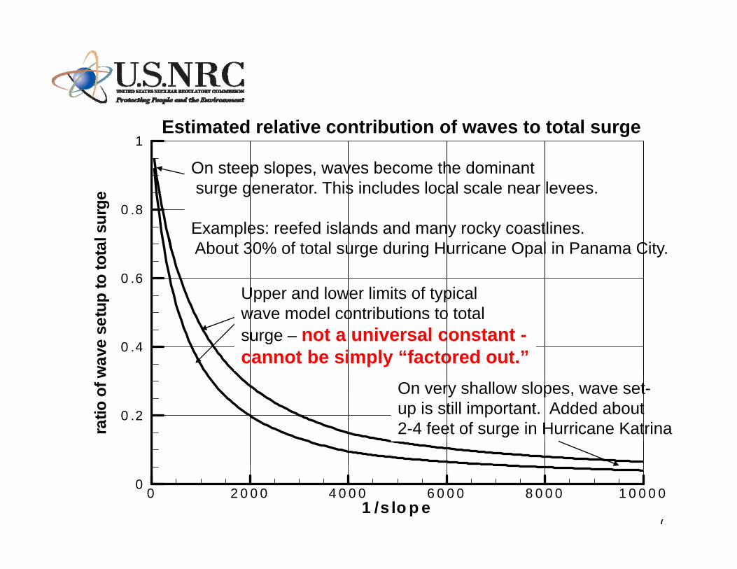
Becomes Asymptotic
2 2
0 ( )
La d a d
w w
c V c Vdx Lg h x g h
ρ ρζρ ρ
⎛ ⎞ ⎛ ⎞= =⎜ ⎟ ⎜ ⎟⎝ ⎠ ⎝ ⎠
∫a d
w a
c p Lh g
ρ λζρ ρ
⎛ ⎞ Δ= ⎜ ⎟⎝ ⎠
NOSt I t it
⎝ ⎠ ⎝ ⎠
*1 x
L Rpζ χ ψ⎛ ⎞
= Δ ⎜ ⎟ 1xR R Rwhenψ
⎛ ⎞ ⎛ ⎞ ⎛ ⎞= ≤⎜ ⎟ ⎜ ⎟ ⎜ ⎟
Storm Intensity
1* * *
xph L
ζ χ ψφ ⎜ ⎟
⎝ ⎠ * * *
*
1 1
x L L L
RwhenL
ψ ⎜ ⎟ ⎜ ⎟ ⎜ ⎟⎝ ⎠ ⎝ ⎠ ⎝ ⎠
⎛ ⎞= >⎜ ⎟
⎝ ⎠
YESStorm Size
* *1
* * *x t
L tRph L t
ζ χ ψ ψφ ∞
⎛ ⎞ ⎛ ⎞= Δ ⎜ ⎟ ⎜ ⎟
⎝ ⎠ ⎝ ⎠* * * 1tt t twhent t t
ψ∞ ∞ ∞
⎛ ⎞ ⎛ ⎞ ⎛ ⎞= ≤⎜ ⎟ ⎜ ⎟ ⎜ ⎟
⎝ ⎠ ⎝ ⎠ ⎝ ⎠ YES⎝ ⎠ ⎝ ⎠
*1 1twhent∞
⎝ ⎠ ⎝ ⎠ ⎝ ⎠⎛ ⎞
= >⎜ ⎟⎝ ⎠
YES
F nctional dependence of the s rge on forcing
Storm Forward Speed
23
Functional dependence of the surge on forcingparameters as they become large-valued.

L ti f 880 b thi h tUpper limit of
historical Gulf of
Given that theuncertainty becomes Location of 880mb on this chart,
given pa = 1013historical Gulf of
Mexico average SST values
uncertainty becomesvery large for very-low probabilities,can we find somecan we find some physical guidancefor focusing onthis range.Schade (2000) showsthe behavior of the PMI under different
this range.
PMI under different assumptions and background fields. Hiswork is in reasonable
t ith th t Maximum Possible Intensity
24
agreement with thatof Tonkin et al. (2000).
Maximum Possible Intensity880 mb ???

NRC Texas ADCIRC Grid
Deterministic-probabilistic approachNRC-Texas ADCIRC Grid
Site of interestSite of interest
25

NRC-Texas ADCIRC Grid
Matagorda
26
In a complex coastal area like this, simple transect models are virtually worthless!!

Storm SuiteRUN No. Fields Available Evaluation Performed
Wind Pres W-lndf P-lndf Rp (nm) Holland B Vf (kt)
RUN025 59.6 880 46.5 904 30-42 1.35-0.9 5.5
RUN026 58 880 42.4 918.6 45-63 1.35-0.9 5.5
RUN027 61.1 870 48.4 893.8 30-42 1.35-0.9 5.5
RUN028 59.4 870 44.4 908.6 45-63 1.35-0.9 5.5
RUN029 61.4 880 47.5 905.8 30-42 1.35-0.9 11
RUN030 59.2 880 44.5 918.6 45-63 1.35-0.9 11
RUN031 62.8 870 49.3 895.8 30-42 1.35-0.9 11
RUN032 60.6 870 46.4 908.6 45-63 1.35-0.9 11
RUN033 64.3 880 54.6 901.9 30-42 1.35-0.9 22
RUN034 61.8 880 50.9 912.3 45-63 1.35-0.9 22
RUN035 65.6 870 55.9 891.9 30-42 1.35-0.9 22
RUN036 63 870 52.7 902.3 45-63 1.35-0.9 22
RUN037 62.3 880 50 902.8 30-42 1.35-0.9 11
RUN038 60 880 44.4 919.6 45-63 1.35-0.9 11
RUN039 63.7 870 51.9 892.8 30-42 1.35-0.9 11
RUN040 61.4 870 46.3 909.8 45-63 1.35-0.9 11
RUN041 65.1 880 55.1 902.8 30-42 1.35-0.9 22
RUN042 62.2 880 48.8 919.6 45-63 1.35-0.9 22
27
RUN043 66.4 870 56.5 892.8 30-42 1.35-0.9 22
RUN044 63.5 870 50.5 909.6 45-63 1.35-0.9 22

Point of interest
28

In this figure, we showthe values of the surgeat Point 59 (inland) plottedagainst the surge valuesat Point 3 (coast) for stormsin which each Point wasi d t dinundated.
Three key points:1) Elevation of Point 59 is around 28.5 ft)2) There seems to be a natural limiter for
the total surge depth in these storms3) A simple transect model cannot reproduce
29
these results.
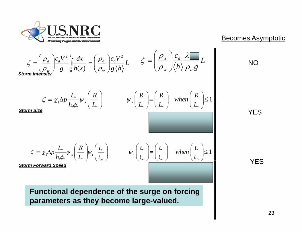
The Future: Other Considerations
A method for determining hurricane flood level extreme value statistics which considers long-term and short-term environmental trends:
• Sea level rise• Hurricane frequency• Hurricane intensity• Landscape evolution
Knutson & Tuleya 2004
30
IPCC 2007

Questions????
31


