
Universitat Ulm
Institut fur Finanzmathematik
Robust Calibration of the Libor Market Model
and
Pricing of Derivative Products
Dissertation
zur Erlangung des Doktorgrades
Dr. rer. nat.
der Fakultat fur Mathematik und Wirtschaftswissenschaften
an der Universitat Ulm
UN
IVERSI TÄ T
ULM·
SC
IEN
DO
·DOCENDO·C
UR
AN
DO
·
vorgelegt von
Dipl.-Math. oec. Dennis Schatz
aus Illertissen
Ulm, 2011

Amtierender Dekan: Professor Dr. Werner Kratz
1. Gutachter: Professor Dr. Rudiger Kiesel, Universitat Duisburg-Essen
2. Gutachter: Professor Dr. Ulrich Rieder, Universitat Ulm
Tag der Promotion: 28.02.2011
Abstract
The Libor market model has established itself as the benchmark model for interest rate
derivatives. If the observed correlation and volatility surfaces cannot be reproduced by
a model, we cannot hope to get meaningful prices, therefore the crucial task, before
it comes to pricing and hedging, is to calibrate the model to given market data. An
overview of the Libor market model is given and it is shown how to obtain a robust
calibration. The big disadvantage of the model is that it cannot reproduce the typically
observed implied volatility smile.
We show how to extend the model to include the market smile by making use of
stochastic volatility. For these stochastic volatility Libor market models a new time
homogeneous skew parametrization is introduced which has the capability of fitting the
observed market data very well. Furthermore a new approximative terminal correlation
formula based on the same parameter averaging technique used for pricing in a stochas-
tic volatility Libor market model is presented. We look at a very robust calibration
procedure and show how to use it if there are no starting values available, here we
introduce some new approximations making it possible to use global optimizers. The
optimal choice of local and global optimizers for each step of the calibration will be
dealt with, especially how to make use of the differential evolution algorithm, which has
attracted interest in the financial community in recent times. Furthermore an analysis
of the robustness of the calibrated parameters over a specific period is performed.
Two extensions to the cross currency Libor market model introduced by Schlogl are
developed. These make use of displacements and stochastic volatility to fit the observed
skew and smile respectively.
The calculation of the Greeks for exotic interest rate derivatives is crucial for hedging
and therefore for trading these products. For a Libor market model this task can only
be fulfilled by means of nontrivial Monte Carlo based methods. One possibility is to use
the proxy simulation scheme method, which makes use of the transition densities of the
discretized processes. When it comes to the calculation of these transition densities in
stochastic volatility models they can only be calculated by means of Fourier inversion.
A new method for the calculation of the weights is developed making use of the con-
ditional independence of the underlying from the stochastic volatility process, which
can be used for any model for which this independence holds. This is also the case
for the new stochastic volatility cross currency model. The developed estimators are
very similar to the estimators for a Libor market model and are fast enough to be used
in everyday practice. We show how the Greeks calculated by these proxy simulation
scheme methods perform compared to the finite differences approximation and show
how the use of Sobol sequences influences the results.

Zusammenfassung
Das Libor Markt Modell hat sich mittlerweile als Benchmark-Modell fur Zinsderivate
etabliert. Wenn ein Modell die am Markt beobachteten Korrelationen und Volatilitats-
oberflachen nicht reproduzieren kann, ist auch nicht davon auszugehen, dass es korrekte
Preise fur exotische Produkte liefert. Deshalb ist die entscheidende Aufgabe zuerst das
Modell an Marktdaten zu kalibrieren, bevor es zur Bewertung und zum Hedgen von
Produkten verwendet werden kann. In der vorliegenden Arbeit wird ein Uberblick uber
das Libor Markt Modell gegeben und gezeigt, wie man eine solche robuste Kalibrierung
erreichen kann. Der große Nachteil des Modells liegt darin, dass es nicht in der Lage
ist den am Markt beobachtbaren Smile abzubilden.
Es wird gezeigt, wie man es durch den Einsatz von stochastischer Volatilitat so erwei-
tern kann, dass auch der Smile kalibriert werden kann. Fur diese Libor Markt Mo-
delle mit stochastischer Volatilitat wird eine neue zeithomogene Parametrisierung fur
die Skews eingefuhrt, welche sehr gut geeignet ist um die Marktdaten zu reprodu-
zieren. Desweiteren wird eine neue approximative Formel fur die Terminale Korrela-
tion prasentiert die auf der gleichen Parametermittelung basiert, wie man sie beim
Preisen in einem solchen Modell anwendet. Eine bekannte robuste Kalibrierungsproze-
dur wird vorgestellt und es wird aufgezeigt, wie man diese verwenden kann wenn
keine Startwerte verfugbar sind. An dieser Stelle werden mehrere Approximationen
eingefuhrt welche den Einsatz von globalen Optimierern erlauben. Wir beschaftigen
uns mit der optimalen Wahl verschiedener lokaler und globaler Optimierer fur jeden
einzelnen Schritt der Kalibrierung und zeigen an welcher Stelle der Differential Evo-
lution Algorithmus, welcher in letzter Zeit die Aufmerksamkeit der Finanzwelt erregt
hat, eingesetzt werden kann. Ausserdem wird die Stabilitat der Parameter uber einen
gewissen Zeitraum hinweg analysiert.
Wir entwickeln zwei Erweiterungen des Cross Currency Libor Markt Modells, welches
von Schlogl eingefuhrt wurde und verwenden dabei ein Displacement um den beobachte-
ten Skew und stochastische Volatilitat um den Smile zu reproduzieren.
Die Berechnung der Griechen fur exotische Zinsderivate ist zum Hedgen und damit
fur den Handel dieser Produkte von entscheidender Bedeutung. Fur ein Libor Markt
Modell muss auf nicht triviale Monte Carlo Methoden zuruckgegriffen werden um diese
Aufgabe zu erfullen. Eine Moglichkeit ist das Proxy-Simulations-Schema Verfahren,
welches von den Ubergangsdichten der diskretisierten Prozesse abhangt. In einem Libor
Markt Modell mit stochastischer Volatilitat konnen diese nur mit Hilfe einer inversen
Fourier-Transformation berechnet werden. Es wird eine neue Methode zur Berechnung
der Gewichte fur das Proxy-Simulations-Schema Verfahren entwickelt, welche die bed-
ingte Unabhangigkeit der Forward-Zinsraten von der stochastischen Volatilitat ausnutzt
und fur alle Modelle anwendbar ist fur die diese Unabhangigkeit gilt. Dies ist insbeson-

dere auch der Fall bei unserem neu entwickelten Cross Currency Libor Markt Modell mit
stochastischer Volatilitat. Die berechneten Schatzer sind sehr ahnlich zu denen in einem
normalen Libor Markt Modell und sind schnell genug um im Tagesgeschaft eingesetzt
werden zu konnen. Ausserdem wird die Performance dieser Proxy-Simulations-Schema
Verfahren im Vergleich zur Finiten-Differenzen Approximation analysiert und gezeigt,
wie der Einsatz von Sobol Quasi-Zufallszahlen die Resultate beeinflusst.


Contents
1 Introduction 1
2 Libor Market Model 7
2.1 Basic Products and Definitions in the Fixed Income Market . . . . . . . 7
2.2 Development of Interest Rate Models . . . . . . . . . . . . . . . . . . . . 8
2.3 Introduction of the Libor Market Model . . . . . . . . . . . . . . . . . . 11
2.3.1 Modeling of Forward Libor Rates . . . . . . . . . . . . . . . . . . 11
2.3.2 Equivalent Specification and Rank Reduction . . . . . . . . . . . 13
2.3.3 Volatility Structure . . . . . . . . . . . . . . . . . . . . . . . . . . 15
2.3.4 Correlation Structure . . . . . . . . . . . . . . . . . . . . . . . . 19
2.3.5 Terminal Correlation . . . . . . . . . . . . . . . . . . . . . . . . . 23
2.4 Pricing of Products . . . . . . . . . . . . . . . . . . . . . . . . . . . . . . 26
2.4.1 Caps and Floors . . . . . . . . . . . . . . . . . . . . . . . . . . . 26
2.4.2 Swaptions . . . . . . . . . . . . . . . . . . . . . . . . . . . . . . . 27
2.4.3 CMS Spread Options . . . . . . . . . . . . . . . . . . . . . . . . . 33
2.4.4 Bermudan Swaptions . . . . . . . . . . . . . . . . . . . . . . . . . 35
2.5 Calibration . . . . . . . . . . . . . . . . . . . . . . . . . . . . . . . . . . 37
2.5.1 Stripping of the Forward Interest Rate Curve . . . . . . . . . . . 38
2.5.2 Volatilities and Correlations . . . . . . . . . . . . . . . . . . . . . 39
2.5.3 Caplet Calibration . . . . . . . . . . . . . . . . . . . . . . . . . . 40
2.5.4 Swaption Calibration . . . . . . . . . . . . . . . . . . . . . . . . . 42
2.5.5 CMS Spread Option Calibration . . . . . . . . . . . . . . . . . . 44
2.5.6 Choosing Products for the Calibration . . . . . . . . . . . . . . . 45
3 Displaced Diffusion Libor Market Model 47
3.1 Modeling of Forward Libor Rates . . . . . . . . . . . . . . . . . . . . . . 47
3.1.1 Equivalence of the Modeling Approaches . . . . . . . . . . . . . . 50
3.1.2 Terminal Correlation . . . . . . . . . . . . . . . . . . . . . . . . . 51
3.2 Pricing of Products . . . . . . . . . . . . . . . . . . . . . . . . . . . . . . 52
3.2.1 Caplets . . . . . . . . . . . . . . . . . . . . . . . . . . . . . . . . 52
3.2.2 Swaptions . . . . . . . . . . . . . . . . . . . . . . . . . . . . . . . 54
3.3 Calibration . . . . . . . . . . . . . . . . . . . . . . . . . . . . . . . . . . 55

viii Contents
4 Stochastic Volatility Libor Market Model 57
4.1 Introduction of the Stochastic Volatility Libor Market Model . . . . . . 57
4.1.1 Modeling of Forward Libor Rates . . . . . . . . . . . . . . . . . . 57
4.1.2 Skew Parametrization . . . . . . . . . . . . . . . . . . . . . . . . 59
4.2 Parameter Averaging . . . . . . . . . . . . . . . . . . . . . . . . . . . . . 61
4.2.1 Effective Skew . . . . . . . . . . . . . . . . . . . . . . . . . . . . 62
4.2.2 Effective Volatility . . . . . . . . . . . . . . . . . . . . . . . . . . 62
4.3 Moment Explosion in Stochastic Volatility Models . . . . . . . . . . . . 64
4.4 Stochastic Volatility Swap Rate Model . . . . . . . . . . . . . . . . . . . 66
4.5 Fourier Transform-based Pricing of Products . . . . . . . . . . . . . . . 67
4.5.1 Caplets . . . . . . . . . . . . . . . . . . . . . . . . . . . . . . . . 67
4.5.2 Swaptions . . . . . . . . . . . . . . . . . . . . . . . . . . . . . . . 69
4.5.3 CMS Spread Options . . . . . . . . . . . . . . . . . . . . . . . . . 70
4.6 A New Approximative Terminal Correlation Formula . . . . . . . . . . . 75
4.7 Calibration to Swaptions . . . . . . . . . . . . . . . . . . . . . . . . . . . 80
4.7.1 Daily Calibration Algorithm . . . . . . . . . . . . . . . . . . . . . 80
4.7.2 Initial Calibration Algorithm . . . . . . . . . . . . . . . . . . . . 84
5 Cross Currency Libor Market Models 89
5.1 Multicurrency Libor Market Model . . . . . . . . . . . . . . . . . . . . . 90
5.2 Displaced Diffusion Extension . . . . . . . . . . . . . . . . . . . . . . . . 92
5.3 Stochastic Volatility Extension . . . . . . . . . . . . . . . . . . . . . . . 94
6 Monte Carlo Based Pricing 99
6.1 Simulation Schemes for the Libor Market Model . . . . . . . . . . . . . 99
6.1.1 Numerical Monte Carlo Simulation Schemes . . . . . . . . . . . . 99
6.1.2 Monte Carlo Error . . . . . . . . . . . . . . . . . . . . . . . . . . 106
6.2 Transition Densities . . . . . . . . . . . . . . . . . . . . . . . . . . . . . 108
6.2.1 Libor Market Model . . . . . . . . . . . . . . . . . . . . . . . . . 108
6.2.2 Displaced Diffusion Libor Market Model . . . . . . . . . . . . . . 109
6.2.3 Stochastic Volatility Libor Market Model . . . . . . . . . . . . . 110
6.2.4 Cross Currency Libor Market Models . . . . . . . . . . . . . . . 112
7 Calculation of Monte Carlo Sensitivities 115
7.1 Overview . . . . . . . . . . . . . . . . . . . . . . . . . . . . . . . . . . . 115
7.1.1 Finite Differences Method . . . . . . . . . . . . . . . . . . . . . . 116
7.1.2 Pathwise Method . . . . . . . . . . . . . . . . . . . . . . . . . . . 118
7.1.3 Likelihood Ratio Method . . . . . . . . . . . . . . . . . . . . . . 119
7.1.4 Proxy Simulation Method . . . . . . . . . . . . . . . . . . . . . . 120
7.1.5 Summary . . . . . . . . . . . . . . . . . . . . . . . . . . . . . . . 122

Contents ix
7.2 Sensitivities in the Libor Market Model . . . . . . . . . . . . . . . . . . 123
7.2.1 Finite Differences Method . . . . . . . . . . . . . . . . . . . . . . 123
7.2.2 Pathwise Method . . . . . . . . . . . . . . . . . . . . . . . . . . . 123
7.2.3 Likelihood Ratio Method . . . . . . . . . . . . . . . . . . . . . . 125
7.2.4 Proxy Simulation Method . . . . . . . . . . . . . . . . . . . . . . 126
7.3 Proxy Greeks in the Extended Models . . . . . . . . . . . . . . . . . . . 128
7.3.1 Displaced Diffusion Libor Market Model . . . . . . . . . . . . . . 128
7.3.2 Stochastic Volatility Libor Market Model . . . . . . . . . . . . . 129
7.3.3 Cross Currency Libor Market Models . . . . . . . . . . . . . . . 131
8 Optimization Algorithms 135
8.1 Levenberg-Marquardt . . . . . . . . . . . . . . . . . . . . . . . . . . . . 136
8.2 Downhill Simplex . . . . . . . . . . . . . . . . . . . . . . . . . . . . . . . 137
8.3 Simulated Annealing . . . . . . . . . . . . . . . . . . . . . . . . . . . . . 138
8.4 Differential Evolution . . . . . . . . . . . . . . . . . . . . . . . . . . . . 140
8.4.1 The Algorithm . . . . . . . . . . . . . . . . . . . . . . . . . . . . 141
8.4.2 Closeup . . . . . . . . . . . . . . . . . . . . . . . . . . . . . . . . 143
8.5 Comparison and Applications . . . . . . . . . . . . . . . . . . . . . . . . 145
9 Numerical Results 147
9.1 Calibration of the Stochastic Volatility Libor Market Model . . . . . . . 147
9.1.1 Bootstrapping of the Forward Rate Curve . . . . . . . . . . . . . 149
9.1.2 Pre-calibration . . . . . . . . . . . . . . . . . . . . . . . . . . . . 151
9.1.3 Main-calibration . . . . . . . . . . . . . . . . . . . . . . . . . . . 154
9.1.4 Parameter Stability . . . . . . . . . . . . . . . . . . . . . . . . . 160
9.2 Sensitivities . . . . . . . . . . . . . . . . . . . . . . . . . . . . . . . . . . 161
9.2.1 Smooth Products - Caplets . . . . . . . . . . . . . . . . . . . . . 162
9.2.2 Non-Smooth Products - Digital Caplets . . . . . . . . . . . . . . 163
9.3 Model Risk . . . . . . . . . . . . . . . . . . . . . . . . . . . . . . . . . . 169
Conclusion 171


1 Introduction
The Libor market model, which was introduced by Brace, Gatarek and Musiela [BGM97],
Miltersen, Sandmann and Sondermann [MSS97] and Jamshidian [Jam97], has not only
gained a wide acceptance in industry and academia, but it has become a market stan-
dard and benchmark model today. Basically it is a discretized version of the famous
Heath Jarrow Morton (HJM) model.1
The main advantages of the Libor market model (LMM) in comparison to the HJM
are that it models the market observable forward Libor rates instead of mathemati-
cally abstract instantaneous forward rates and derivative pricing is much easier in that
framework, especially caplets and swaptions can be priced consistently with the long-
used formulas of Black, which are still a market standard.2
A major problem of the LMM is that it cannot capture the observed market smile.
Not incorporating the skew or smile may result in severe losses when using such a model
to price exotic products. Therefore many extensions have been proposed to incorpo-
rate the skew or smile in existing literature. Displacements have been introduced, CEV,
Levy and stochastic volatility models have been proposed to deal with the problem.
The main steps taken in skew and smile modeling for the Libor market model are the
following:
• Local Volatility: The first steps towards incorporating skew features in a LMM
were made by Andersen and Andreasen [AA00] by using local-volatility processes
for the Libor rates.
• Levy: Attempts to deal with the smile problem by making use of jump diffusion
processes were for example undertaken by Glasserman and Kou [GK03] and Be-
lomestny and Schoenmakers [BS06].
General Levy Libor models were studied by Eberlein and Ozkan [Ez05], but the
calibration, especially a robust calibration of these models is a tough task.
• Stochastic Volatility: Models making use of stochastic volatility to incorporate
the market smile were introduced among others by Andersen and Brotherton-
Ratcliffe [ABR05], Joshi and Rebonato [JR03], Piterbarg [Pit03b] and Wu and
Zhang [WZ06]. A major problem of many stochastic volatility models is that in
1For details see for example Brigo and Mercurio [BM06].2The market quotes caps and swaptions in Black volatilities.

2 1 Introduction
order to introduce a skew they correlate the SDEs driving the underlying for-
ward Libor rates and the stochastic volatility. Andersen and Brotherton-Ratcliffe
[ABR05] and later Piterbarg [Pit03b] mix the approaches of displaced diffusion for
the skew and stochastic volatility for the smile. From a calibrational point of view,
Andersen and Brotherton-Ratcliffe and the Piterbarg approach are preferable as
in these cases the stochastic volatility process is independent of the forward Libor
rates. Furthermore many researchers believe that skews and smiles are caused
by different market features and therefore they should be modelled separately.
The displaced diffusion setting results in easier valuation formulas than the CEV
setting and works perfectly in combination with stochastic volatility.
If we put ourselves in the position of a trader we must ask the following questions when
we want to sell a product.
• What is the price I am willing to sell it for?
• How can I hedge myself?
The first step we have to take in order to answer these questions is to choose a model.
Many exotic products, like products with callable features, are difficult to handle and
therefore the simple, first generation interest rate models like Hull-White or Black-
Karasinsky should not be used. The problem is that they cannot be calibrated to a
rich enough set of market instruments. One has to use second generation models, like
the Libor market model, that are capable of calibrating a whole volatility surface.
A well calibrated model which is capable of capturing the important market features in
combination with a Monte Carlo pricing engine3 then takes care of the first task. We
will show how to fulfill this task in Chapters 2-6.
For the second task we face, at least for many products, the problem that there are
no natural hedges available and therefore hedging usually comes down to calculating
the Greeks and trying to neutralize the Greeks of the portfolio. The calculation of
the Greeks by means of Monte Carlo methods is topic of Chapters 6 and 7. There-
fore a property a good model should fulfill is the possibility to calculate the Greeks.
While there is a broad literature on how to calculate the Greeks in a Libor market
model (LMM) and the displaced diffusion Libor market model (DDLMM) there is still
a lack of these methods for the LMMs with smile features. The correlation of the
Libor rates with the stochastic volatility processes in the stochastic volatility Libor
market models (SVLMMs) poses severe problems when we actually want to calculate
the Greeks and therefore we prefer one of the uncorrelated models, i.e. Andersen and
Brotherton-Ratcliffe [ABR05], or Piterbarg [Pit03b]. From a calibrational point of view
the Piterbarg approach is preferable as the calibration can be split up in a two step
3If there are no analytical formulas available.

3
process, therefore we will concentrate on this model in the smile section.
If the calibrated parameters vary too much on a daily basis we have to adjust the hedg-
ing portfolio very often, therefore we should make sure that the calibration obtains
robust parameters.
Another topic we will deal with are Cross Currency models. We start with the model
introduced by Schlogl [Sch02] and then develop some generic extensions to arrive at a
joint model where the individual markets are also in the spirit of the Piterbarg model
and where we are still able to calculate the Greeks.
An overview on the structure and the contributions of the thesis is given in Table 1.1.
Chapter Content Contribution
Chapter 2 LMM
Chapter 3 DDLMM Comparison of versions of different DDLMMs
Chapter 4 SVLMM Time homogeneous skew parametrization
Terminal correlation formula
Approximations for the effective volatility
Global calibration algorithm
Chapter 5 CCLMM Generic DDCCLMM extension of CCLMM
Generic SVCCLMM extension of CCLMM
Chapter 6 MC Simulation Transition densities for the models
Chapter 7 MC Greeks Proxy Greeks for SVLMM
Proxy Greeks for CCLMMs
Chapter 8 Opt Algorithms
Chapter 9 Numerical Results Analysis forward curve interpolation/extrapolation
Analysis of calibration quality
Comparison finite differences vs proxy Greeks
Comparison Sobol sequences vs Mersenne-Twister
Analysis of stochastic volatility proxy Greeks
Analysis impact of displacement & stoch volatility
Table 1.1: Topics and contributions of the thesis.
Structure and contributions of this thesis
• In Chapter 2 we will give an introduction to the interest rate market before we
have a close look at the Libor market model.
We look at correlation and volatility parametrizations, which we will also use
for the displaced diffusion and stochastic volatility Libor market models. The
concepts of instantaneous and terminal correlation are introduced and we state

4 1 Introduction
an approximation for the terminal correlation. Furthermore we show how to price
analytically the products we want to use for calibration and how to proceed in
order to get a robust calibration. This section serves as a basis for the extended
models later on and can be seen as a collection of the main literature available
up to date.
• The incorporation of the market skew will be topic of Chapter 3, where we extend
the Libor market model by two different versions of displacements and show again
how the prices are calculated for the basic products.
Furthermore we will show that the displacements used by Andersen Brotherton-
Rathcliff and Piterbarg can in some sense be seen as equivalent by showing that
the models induce the same dynamics. We briefly discuss how to price the basic
products and hint how to calibrate the displaced model to market data.
• In Chapter 4 we will show how we can extend the Libor market model to incor-
porate smile features.
The introduction of a new time homogeneous skew parametrization will be part
of this chapter, before we will introduce the parameter averaging techniques used
to calculate the effective skew and effective volatility. After that we look at
some common problems that might occure when it comes to pricing in stochastic
volatility models and with all that at hand we will deal with the pricing of the
basic products.
We introduce a new approximative terminal correlation formula for stochastic
volatility models which might be useful for calibration and in the last part we
will show how to approximate the effective volatility to speed up the global or ini-
tial calibration. While the author of the paper on the presented model provides
a calibration routine which works perfectly well in case we have good starting
parameters, the routine is too slow for a global calibration. With this approxi-
mation we can make use of global optimizers to find the optimal parameters. A
detailed description of the calibration to swaptions concludes the chapter.
• The cross currency Libor market model (CCLMM) introduced by Schlogl [Sch02]
will first be presented in Chapter 5, before we extend it to a displaced diffusion
(DDCCLMM). Finally we extend it to a new stochastic volatility (SVCCLMM)
setting in the spirit of the Piterbarg model from Chapter 4 with a foreign exchange
rate following a similar process as the forward Libor rates. We derive all of the
necessary dynamics under the terminal measure to simulate the underlyings later
on and to calculate the sensitivities.
• Chapter 6 is devoted to Monte Carlo techniques for the Libor market model and
its extensions.

5
Furthermore we will calculate the transition densities for the models, which are
necessary to calculate the Monte Carlo Greeks in the next chapter.
• We give an overview on existing Monte Carlo methods for Greeks estimation and
apply them to the Libor market model in Chapter 7. After that we show how
to apply the proxy Greeks method to all of the introduced models. Especially
we show a new way how to apply it to a stochastic volatility LMM in case of an
independent stochastic volatility process.
• The introduction of some numerical optimizers for the calibration of the models
will be topic of Chapter 8. We will have a look at different local and global
optimizers and compare their features. The differential evolution algorithm is
presented in more detail as it has been introduced to solve financial problems only
recently and we will show how we can apply it to the calibration of a stochastic
volatility model in this thesis.
• Finally we will present some numerical results in Chapter 9. First we show how
to obtain the initial forward rate curve, before we deal with the initial/global
calibration of the stochastic volatility Libor market model presented in Chapter
4. The actual fitting qualities of the model will be analysed and we look at the
robustness of the obtained parameters.
The second part is devoted to the calculation of the Greeks, where we compare
the finite differences method to the proxy Greeks method. Furthermore we have
a closer look at the effect of using Sobol sequences and analyse the new stochastic
volatility estimator.
In the last part of the chapter we look at the impact of the displacement and the
stochastic volatility on the calibration quality.
Literature Overview
The literature that might be useful to understand and implement these models is very
broad, therefore we group it in four categories, which we list in the following. We
suppose that the reader is familiar to the basic concepts of stochastic calculus and fi-
nancial mathematics. Excellent introductions to these topics can be found in Bingham
and Kiesel [BK04a], Shreve [Shr04] and Øksendal [Øks03].
Basic introduction to the Libor market model:
There are quite a few books and articles dealing with the Libor market model, for
example Brigo and Mercurio [BM06], Rebonato [Reb02], Schoenmakers [Sch05], Brace
[Bra07], Fries [Fri07], Gatarek et al. [GBM07], Rebonato [Reb04] and many more. We
think the books of Rebonato, Fries and especially Brigo and Mercurio are a very good

6 1 Introduction
starting point.
The introductory chapters of this dissertation mainly follow Brigo and Mercurio [BM06],
Rebonato [Reb02] and Schoenmakers [Sch05].
Smile Extensions of the Libor market model:
A good overview on this topic can be found in Svoboda-Greenwood [SG07], Meister
[Mei04] and again Brigo and Mercurio [BM06].
Some specific more detailed promising approaches are given in Piterbarg [Pit03b], An-
dersen [ABR05], Joshi and Rebonato [JR03] and Wu and Zhang [WZ06].
Numerical methods:
In Press [Pre07] we find a very good overview on many numerical topics, furthermore
we suggest to read Jackel [Jac02].
An introduction to the optimization algorithms is given in Nocedal [NW00] and again in
Press [Pre07]. For the Monte Carlo simulation methods we suggest the books of Glasser-
man [Gla04], Duffy and Kienitz [DK09] and Kloeden, Schurz and Platen [KSP07].
For the calculation of the Greeks we suggest the paper of Glasserman [GZ99], the works
of Fries [Fri07], [Fri05], [FJ08] and [FK06] and the papers of Joshi, especially Denson
and Joshi [DJ09]. For the theoretical background on these topics we suggest Kloeden
and Platen [KP99] and Protter [Pro05].
Implementation:
For the implementation of the models we used the open source library QuantLib http:
//quantlib.org/ as a basis. As there is virtually no documentation for QuantLib
available the reader should get familiar with the advanced object oriented concepts of
C++ programming first, before using the library. Some books we recommend are Duffy
[Duf04], Duffy [Duf06], Duffy and Kienitz [DK09] and Joshi [Jos08].

2 Libor Market Model
Before we start describing the Libor market model (LMM) we give a brief introduction
to the basic definitions and notations in the fixed income market and describe the
historical development of the interest rate models. We go on with a description of the
instantaneous volatility and correlation parametrizations used to specify the model,
before we handle the pricing of some basic products used to calibrate the model. Then
we have a look at a Bermudan swaption as an example of an exotic product, which can
only be valued by means of Monte Carlo simulation. At the end of the chapter we deal
with the calibration of the model to market quotes. In this introductory part we will
follow closely the book of Brigo and Mercurio [BM06] and Rebonato’s book [Reb02].
2.1 Basic Products and Definitions in the Fixed Income Market
First of all we will introduce the basic notation and the basic products that we will
deal with throughout this thesis.
Definition 2.1.1
The basic products and instruments are defined as follows
• A contract which pays one at maturity T is called a zero coupon bond, or zerobond
and its time t value is denoted by P (t, T ) with t < T . If we suppose to work with
simply-compounded interest rates we get
P (t, T ) =1
1 + L(t, T )τ(t, T ),
where L(t, T ) denotes the Libor rate defined below and τ(t, T ) is the time difference
in years making use of the appropriate day count convention.1 The Libor rate is
the discretely paid interest rate from t to T and is introduced below.
• The London Interbank Offered Rate (Libor) is defined as
L(t, T ) :=1− P (t, T )
τ(t, T )P (t, T ).
The BBA British Bankers’ Association publishes the following rates: Overnight,
1 week, 2 weeks, 1-12 months.
1For an overview of different daycount conventions the interested reader is referred to Zagst [Zag02].

8 2 Libor Market Model
• The forward price of a zero coupon bond is given as
FP (t, T1, T2) =P (t, T2)
P (t, T1), (2.1)
with 0 ≤ t ≤ T1 < T2.
• If we work on a time grid 0 ≤ t ≤ T0 < T1 < · · · < TM , the forward Libor
Fi(t) := F (t, Ti−1) := F (t, Ti−1, Ti), which is the simply-compounded interest rate
between Ti−1 and Ti, is given as
P (t, Ti)
P (t, Ti−1)=
1
1 + F (t, Ti−1)τ(Ti−1, Ti)=
1
1 + Fi(t)τi, (2.2)
with τi = τ(Ti−1, Ti), ∀i = 1, ...,M .
2.2 Development of Interest Rate Models
Before we actually start describing the Libor market model, we want to give a brief
overview of the development of interest rate or rather yield curve modeling. In the fol-
lowing we also address the question why one might want to use a Libor market model.
Before the yield curve models became popular Black-like formulas were used to price
interest rate derivatives like caplets and swaptions. They became a market standard in
these days, which is also the reason why the cap and swaption prices are still quoted in
Black volatilities. We do not want to go into details about these models at this place
and move on to the development of the first yield curve models.2
We assume that the bank account with initial value B(0) = 1 follows the following
dynamics
dB(t) = r(t)B(t)dt,
where r(t) is a positive function, which gives us the value of the bank account as
B(T ) = exp
(∫ T
0r(s)ds
),
for some T > 0. This means that the instantaneous rate r(t), which we will call briefly
the short rate, is the rate at which the bank account accrues continuously.
In many markets like for example equity or foreign exchange the existing models assume
this bank account to be deterministic, i.e. the short rate is believed to be a deterministic
function of time. This assumption stems from the fact that the main variability in these
markets comes from other sources than from varying interest rates and one does not
2For more details on historical developments see Rebonato [Reb02] and [Reb03].

2.2 Development of Interest Rate Models 9
want to make the models more complicated than necessary. We want to deal with
products that depend on the variability coming from the interest rate market. So we
will model the variability coming from the interest rates and therefore we have to use
a stochastic short rate. These kinds of models are called short rate models and were
one of the first models for the interest rate market. Of special interest are the so-called
affine models as there are analytical prices for zero coupon bonds readily available.
There exists a broad literature covering short rate models, for a good overview see
Brigo and Mercurio [BM06], or Cairns [Cai04].3
Some examples of these models are Vasicek (1977), Dothan (1978) and Cox, Ingersoll
and Ross (1985), which we will briefly call the CIR model. For example the CIR model
assumes the following dynamics for the short rate
dr(t) = κ(θ − r(t))dt+ σ√r(t)dW (t), r(0) = r0 > 0.
All of these models can be extended to multi factor models giving them additional
degrees of freedom for the calibration to market quotes. Later some models with time
dependence have been introduced, e.g. Hull and White (1990) and Black and Karasin-
ski (1991). Furthermore jumps have been introduced to model the dynamics of the
short rate.4
A problem that all these models have in common is that the discount curve is given
at the moment we specify the parameters. So we have to calibrate the model to the
discount or yield curve and cannot use it as an input. This makes it possible for these
models to detect arbitrage possibilities in trading the products building the yield curve,
but makes it hard for these models to handle more advanced exotic products relying
on the yield curve which should be fitted perfectly in this case.5
To solve the problem of the endogenously given yield curve, in 1992 a different approach
was introduced by Heath, Jarrow and Morton, which was based on a model by Ho and
Lee (1986). The so-called HJM model takes the whole yield curve as exogenous input
and specifies the dynamics for every point on the yield curve, instead of just specifying
the dynamics of the short rate. The instantaneous forward rate is defined as
f(t, T ) = −∂ lnP (t, T )
∂T,
and the dynamics for the instantaneous forward rates in the HJM model are given as
df(t, T ) = α(t, T )dt+ σ(t, T )dW (t), f(0, T ) = fM (0, T ), ∀ 0 ≤ t ≤ T.3For more details see Duffie, Pan and Singleton [DPS00] and Bolder [Bol01].4Descriptions of these models can all be found in Brigo and Mercurio [BM06].5The perfect fit to the yield curve can be achieved for the easier early day models by introducing
a deterministic function which is added to the short rate. Examples for this method are given in
Brigo and Mercurio [BM06], e.g. the CIR++ model.

10 2 Libor Market Model
Here fM (0, T ) is the market instantaneous forward rate curve at time 0, α : R2 7→ R
and σ : R2 7→ RN with σ(t, T ) = (σ1(t, T ), ..., σN (t, T )) are two functions and W =
(W1, ...,WN )ᵀ is a N -dimensional Brownian motion. Furthermore some arbitrage re-
strictions are imposed on α. As soon as we specify the volatility σ the function α is
determined by the arbitrage restrictions. So the HJM model models every single point
on the forward curve in contrast to the short rate models, which only specify the dy-
namics of the short rate. The dynamics for all other instantaneous forward rates of the
curve are then given implicitly.
The models we introduced so far have in common that the analytical pricing formulas
for more complicated products like caps and swaptions6, if they exist at all, are quite
complicated and especially computationally expensive to calculate. Furthermore the
short rate models have problems with fitting a whole volatility term structure. But the
main drawback is that none of them is consistent with the market Black formulas for
caplets and swaptions.7
A way out of this dilemma is to use a Libor market model also sometimes referred
to as lognormal forward-Libor model (LFM), or we use a swap market model (SMM)
which is also sometimes called lognormal forward-swap model (LSM). In a LFM/LSM
the Libor/swap rates are modelled as lognormal processes under their specific, natural
measure. This approach also makes them incompatible to each other, because a swap
rate is a weighted sum of Libor rates with stochastic weights and therefore if the Libor
rates are lognormal under their natural measure the swap rates cannot be lognormal
under their individual measures at the same time and vice versa. But actually they are
not ‘far away’ from being lognormal. A more detailed treatment of this discrepancy
can be found in Brigo and Mercurio [BM06, page 244].
The Libor market model is actually very similar to the HJM, to be precise it is a special
case of the HJM. In a LMM we do not evolve the whole (unobservable) yield curve,
but we discretize it with some tenor τ > 0 and only evolve the discretized forward
rates. These forward rates can be stripped from the market quotes of deposits, floating
rate agreements (FRAs), futures and swaps and are therefore more or less directly ob-
servable in contrast to the instantaneous forward rates. This stripped yield curve then
serves as a market input, so we have an exogenous model.
Another feature of the Libor market model is that, as the yield curve is a market in-
put, we can use all the parameters which specify the model to calibrate the volatility
6The cap and swaption markets are the two main derivative markets in the interest rate world and
therefore we might want to calibrate the model to them.7For the market Black formulas for caplets and swaption the underlying swap rate or Libor rate is
assumed to be lognormal.

2.3 Introduction of the Libor Market Model 11
and correlation structure obtained by the cap and swaption market quotes. Besides this
feature it allows for a quick and easy calibration to the cap and swaption market quotes.
The biggest problem of the Libor market model is that it cannot reproduce the observed
market skew and smile in the cap and swaption market. But there is a number of
extensions of the Libor market model which address exactly this drawback by including
for example displacements, stochastic volatility or jumps in the dynamics.8 Some of
these will also be the topic of this thesis. In the next subsection we introduce the Libor
market model before we extend it by different versions of displacements in the next
chapter and after that we will include stochastic volatility in our dynamics.
For choosing one of these models, we have to ask the question:”For what do we want
to use it for?“
• If we want to detect arbitrage opportunities in the yield curve we choose a short
rate model.
• If we want to price exotic products which are hedged by FRAs, swaps, caplets
and swaptions we rather choose a market model.
• If the product depends on the market skew or smile of the caplets and swaptions
we choose one of the extensions that we just stated.
2.3 Introduction of the Libor Market Model
In contrast to a short rate model, where the underlying is an unobservable instantaneous
interest rate, the so-called short rate, the Libor market model models more or less
observable forward Libor rates.9 The Libor rates starting today are fixed and all of the
forward Libor rates are stochastic. After each period, which has to be chosen at the
beginning when we set up the model10, we fix another Libor rate and therefore need to
evolve one less.
2.3.1 Modeling of Forward Libor Rates
Now we come to the modeling of the forward Libor rates, or short forward Libors. The
current subsection and the following two subsections where we describe the instanta-
neous volatility and correlation are the crucial part of defining the Libor market model.
8For an overview see Svoboda-Greenwood [SG07], Meister [Mei04] and Brigo and Mercurio [BM06].9Actually they have to be stripped from directly observable products like deposits, FRAs, futures and
swaps. For more details on the stripping algorithm see Section 2.5.1.10We have to choose the tenor of the model. Appropriate choices are three months, six months or a
twelve months setting.

12 2 Libor Market Model
We model M forward rates as lognormal random variables under their respective for-
ward measure.
To be precise, in the Libor market model the dynamics of each forward Libor Fk under
its individual forward measure11 Qk is given as
dFk(t) = σk(t)Fk(t)dWk(t), ∀k = 1, ...,M.
For simulation purposes we need to fix one measure and look at the dynamics of the
forward Libors under one forward measure Qi. The dynamics are given by the following
propostion.
Proposition 2.3.1 (Forward measure dynamics in the LMM)
Let 0 ≤ t < T0 < T1 < · · · < TM and τi = τ(Ti−1, Ti) = Ti − Ti−1, for i = 1, ...,M .
Under the forward measure Qi we have the following dynamics of the forward Libor
rate Fk with k ∈ 1, ...,M
• i = k, t ≤ Tk−1 :
dFk(t) = σk(t)Fk(t)dWk(t)
• i < k, t ≤ Ti :
dFk(t) = σk(t)Fk(t)k∑
j=i+1
ρk,jτjσj(t)Fj(t)
1 + τjFj(t)dt+ σk(t)Fk(t)dWk(t)
• i > k, t ≤ Tk−1 :
dFk(t) = −σk(t)Fk(t)i∑
j=k+1
ρk,jτjσj(t)Fj(t)
1 + τjFj(t)dt+ σkFk(t)dWk(t)
Here Wk is the k-th component of the M -dimensional correlated Brownian motion W
under Qi with
dWi(t)dWj(t) = ρi,jdt, ∀i, j = 1, ...,M.
The bounded deterministic functions σk(.) represent the volatility of the forward
Libor processes Fk for all k = 1, ...,M . The specification of this function is one crucial
modeling approach. We may choose this function to be piecewise constant, piecewise
linear, or use some parametric approach. We will deal with this volatility function in
Section 2.3.3. Furthermore we have to specify the instantaneous correlation structure
ρi,j . Actually one can also choose the correlation to be time dependent, i.e. ρi,j(t)
instead of ρi,j . This will be done in Subsection 2.3.4.
11This means we choose P (0, Tk) as numeraire for modeling Fk for all k ∈ 1, ...,M.

2.3 Introduction of the Libor Market Model 13
Remark 2.3.2
By a direct application of Ito’s formula we can calculate the dynamics of lnFk(t) under
Qk as follows
d lnFk(t) = −σk(t)2
2dt+ σk(t)dWk(t), t ≤ Tk−1.
Remark 2.3.3
If we choose the terminal measure for simulation purposes, we have the problem that
the first forward Libor rates have a larger drift term and so if we freeze the drift it has
a bigger impact on the short end than it has on the long end. There is a way out by
using a varying numeraire, which we will introduce in the following.
We now introduce a discretely rebalanced bank account Bd which can be seen as an
alternative to the continuously rebalanced bank account Bc(t) with the dynamics given
by dBc(t) = r(t)Bc(t)dt.
Definition 2.3.4
A discretely rebalanced bank account Bd(t), which is rebalanced at the times of the
discrete tenor structure is given by
Bd(t) =P (t, Tβ(t)−1)∏β(t)−1
j=0 P (Tj−1, Tj)=
β(t)−1∏j=0
(1 + τjFj(Tj−1))P (t, Tβ(t)−1),
where β(t) denotes the index of the first forward rate that has not expired by time t.
If we choose Bd as numeraire we get the so-called spot Libor measure.
Proposition 2.3.5 (Spot Libor measure dynamics in the LMM)
The dynamics of the forward rate Fk under the spot Libor measure Qd are given as
dFk(t) = σk(t)Fk(t)
k∑j=β(t)
τjρj,kσj(t)Fj(t)
1 + τjFj(t)dt+ σk(t)Fk(t)dW
dk (t),
where W dk (t) is the k-th component of the M -dimensional correlated Brownian motion
W d under Qd with dW di (t)dW d
j (t) = ρi,jdt.
2.3.2 Equivalent Specification and Rank Reduction
The results of this section are mainly taken from Schoenmakers [Sch05] and Fries [Fri07].
We assume that we have M forward rates and that their dynamics under the respective
individual forward measure Qk are given as follows
d lnFk(t) = −σk(t)2
2dt+ σk(t)dWk(t), t ≤ Tk−1, (2.3)

14 2 Libor Market Model
with a M -dimensional correlated Brownian motion W (t) = (W1(t), ...,WM (t)) with
dWi(t)dWj(t) = ρi,j(t)dt and one dimensional volatility functions σi : [0, Ti−1] 7→ R+
for i = 1, ...,M .
If we make sure that for the vector γi(t) ∈ RM the following holds
σi(t) := |γi(t)| =
√√√√ M∑k=1
γ2i,k(t), 0 ≤ t ≤ Ti−1, 1 ≤ i ≤M
and that we have for the instantaneous correlation
ρi,j(t) =γᵀi (t)γj(t)
|γi(t)||γj(t)|, 0 ≤ t ≤ min(Ti−1, Tj−1), 1 ≤ i, j ≤M,
then (2.3) is equivalent to
d lnFk(t) = −γᵀk(t)γk(t)
2dt+ γᵀk(t)dZ(t), t ≤ Tk−1,
with a standard M -dimensional Brownian motion Z(t) = (Z1(t), ..., ZM (t)), which
means that dZi(t)dZj(t) = 0dt.
For the drift we get
µi(t) = σi(t)
k∑j=i+1
ρi,j(t)τjσj(t)Fj(t)
1 + τjFj(t)dt
=
k∑j=i+1
τjFj(t)
1 + τjFj(t)γᵀj (t)γi(t)dt.
In order to get an equivalent model we set
γi(t) = σi(t)fi(t),
with
ρij(t) =
M∑k=1
fi,k(t)fj,k(t) = fᵀi (t) · fj(t),
where the vectors fi(t) are normalized, i.e. |fi(t)| = 1. Therefore we immediately see
that
|γi(t)| = |σi(t)fi(t)| = σi(t)|fi(t)| = σi(t).
So there exists a M ×M matrix F = (fi,j)i,j=1,...,M such that
dWi(t) =
M∑k=1
fi,k(t)dZk(t), dW (t) = F (t)dZ(t).
Furthermore if we multiply F by an orthonormal matrix Q ∈ RM×M , with QQᵀ = IM
and IM being the M -dimensional identity matrix, we get the same scalar volatility.

2.3 Introduction of the Libor Market Model 15
Rank Reduction
In order to reduce the rank we have a look at the correlation matrix, perform a principal
component analysis and consider only the eigenvectors of the d largest eigenvalues.
We suppose to have a M -dimensional correlated Brownian motion W = (W1, ...,WM )ᵀ
with correlation matrix R(t) = (ρi,j(t))i,j=1,...,M with
ρi,j(t)dt = dWi(t)dWj(t).
If we want to reduce the number of factors driving the model we can do a principal
component analysis and only use the eigenvectors corresponding to the largest eigen-
values of the matrix R(t) and then only use d ≤M factors.
We suppose to have a matrix R(t) which is symmetric and positive-semidefinite imply-
ing for the eigenvalues λ1(t) ≥ λ2(t) ≥ ... ≥ λM (t) ≥ 0 with corresponding eigenvectors
v1(t), ..., vM (t). Then we know that
∃V (t) ∈ RM×M : R(t) = V (t)D(t)V ᵀ(t),
with
D(t) := diag(λ1(t), λ2(t), ..., λM (t)) and V ᵀ(t)V (t) = I,
where I denotes the M ×M identity matrix. So we can write
dW (t) = V (t)√D(t)dU(t) = F (t)dU(t),
with a M -dimensional standard Brownian motion U and F (t) = (f1(t), ..., fM (t)). If
we define the renormalized matrix
F (t) := (f r1 (t), ..., f rd (t)), with f ri,j :=fi,j
(∑d
k=1 f2i,k)
1/2,
we can write
dW (t) = F (t)dZ(t),
with a d-dimensional standard Brownian motion Z. Hence a M -dimensional correlated
Brownian motion W depending on d factors, i.e. a M -dimensional d-factorial Brownian
motion.
For more details on rank reduction see Fries [Fri07].
2.3.3 Volatility Structure
What we want is a term structure of volatilities that fits the market as good as possible
and besides that is also as time homogeneous as possible.12 Time homogeneity means
12Furthermore it should be granted that the value of the volatility stays real and positive.

16 2 Libor Market Model
that the term structure at time t > 0 should have the same shape as today. In the
existing literature we can find many different possibilities how to specify the volatility
structure. There are basically two classes of approaches for practical applications, the
piecewise constant and the parametric (continuous) approaches. We will now briefly
introduce a promising piecewise constant volatility term structure before moving on to
the parametric approach that we choose for our model and computations.
Piecewise Constant Approach
There are quite a few possibilities to choose piecewise constant volatilities for an
overview see Brigo and Mercurio [BM06, page 210]. We do not want to present all
of these possibilities, but rather have a glance at one promising approach.13 As the
name already suggests in this case we assume that the volatility is constant between
two Libor fixing dates, i.e we assume
σk(t) = σk,β(t) := Φkψk−(β(t)−1), ∀t ∈ [0, Tk−1],
where β(t) denotes the first forward rate that has not expired yet. The squared caplet
volatility is defined by
v2i,cpl :=
1
Ti−1
∫ Ti−1
0σ2i (t)dt.
The squared caplet volatility multiplied by time can then be calculated as follows
v2i := Ti−1v
2i,cpl =
∫ Ti−1
0σ2i (t)dt = Φ2
i
i∑j=1
τj−2,j−1 ψ2i−j+1.
By choosing
Φ2i =
(vMKTi )2∑i
j=1 τj−2,j−1 ψ2i−j+1
we make sure that we fit all caplets perfectly at the costs of losing time homogeneity.
(vMKTi )2 denotes the caplet market quotes. We have a time homogeneous part ψ and
a time inhomogeneous part Φi, because every forward rate Fi has its own Φi.
This can be extended by using a finer, or even better an adapted grid. The problem
is that we will get many parameters for the calibration later. In the standard case we
will have to calibrate M parameters for ψ and another M factors for Φ, so we have 2M
parameters in total.
On the other hand in this case the calibration is rather a stripping algorithm in case of
the Libor market model, therefore a fast calibration is possible. But if we use some of
the extensions, for example a stochastic volatility Libor market model, the high number
of parameters might become problematic for this calibration.
13This corresponds to the fifth approach in Brigo and Mercurio [BM06, page 211].

2.3 Introduction of the Libor Market Model 17
Parametric Approach
We decide to choose the following continuous approach, because it seems very promising
to us. Under some constraints it guarantees that the volatility term stucture stays
positive and we can easily control the deviation from being a time homogeneous model.
Furthermore we can capture all the typical shapes of the volatility structure that can
be observed in the market.
We choose the continuous deterministic function σi(t) as follows
Φiψ(Ti−1 − t; a, b, c, d) := Φi
([a+ b(Ti−1 − t)]e−c(Ti−1−t) + d
),
σi(t) := Φiψ(Ti−1 − t; a, b, c, d). (2.4)
So again we have a time homogeneous part ψ(Ti−1− t; a, b, c, d), which depends on the
time until the forward Libor is fixed, i.e. Ti−1 − t and a time inhomogeneous part Φi,
which only depends on Ti−1, so every forward rate Fi again has its own Φi. If we re-
strict the correction factor Φi to be close to one,14 we get an almost time homogeneous
volatility structure.
So we have M + 4 parameters. For the four main parameters a, b, c, d we have to im-
pose the following constraints to get a well-behaved, valid, meaningful instantaneous
volatility.
Constraints for the parameters:
1. a+ d > 0,
2. d > 0,
3. c > 0.
If we look at the extreme cases t → T or T → ∞, we get an interpretation of these
constraints.
Let t→ T then we have
σ(t) = a+ d,
so we have that a+ d approximately describes the situation where the forward Libor is
just before its expiration. As the volatility should never be negative, this gives rise to
the first constraint. It can be interpreted as the instantaneous volatility of the forward
14We should at least make sure that all Φi’s have almost the same value 6= 0. The more they deviate
from each other the more time homogeneity is lost.

18 2 Libor Market Model
Libor rate with the shortest maturity.
If T →∞ we have
σ(t) = d,
so d approximately describes the instantaneous volatility of the longest maturity, giving
rise to the second constraint.
Furthermore (b− ca)/cb is the location of the extremum15 of the humped curve.
Figure 2.1: Typically observed market hump of ATM caplet volatilities and instanta-
neous volatilities.
Again we have v2i = Φ2
i
∫ Ti−1
0 σi(t)2dt.
As for the piecewise constant approach the Φi’s can be used to achieve a perfect fit to
the observed volatility surface by setting
Φ2i :=
(vMKTi )2∫ Ti−1
0 σi(t)2dt. (2.5)
By choosing the Φ’s this way we only have to calibrate four of the M + 4 parameters
in our calibration routine.
Besides getting a smooth volatility function, which is capable of fitting the market in
normal and in excited times, this parametrization makes sure that the model is as time
homogeneous as we want it to be and is easy to control in time. A main advantage
of this approach is that we can easily calculate the integral over two instantaneous
volatility functions.
We will need to do that later when we want to calculate the model implied volatility
and the terminal correlation. In this case we need to evaluate the following integral∫ T
tρi,j(s)σi(s)σj(s)ds.
15If b > 0 we have a maximum.

2.3 Introduction of the Libor Market Model 19
If we assume a time independent correlation matrix and w.l.o.g. Ti−1 ≤ Tj−1 this comes
down to16
∫ Ti−1
tρi,j(s)σi(s)σj(s)ds = ρi,j
∫ Ti−1
tσi(s)σj(s)ds =
=ρi,j4c3
(4ac2d(exp[c(t− Tj−1)] + exp[c(t− Tj−1)]) + 4c3d2t
−4bcd exp[c(t− Ti−1)][c(t− Ti−1)− 1]− 4bcd exp[c(t− Ti−1)][c(t− Tj−1)− 1]
+ exp[c(2t− Ti−1 − Tj−1)]2a2c2 + 2abc[1 + c(Ti−1 + Tj−1 − 2t)]
+b2[1 + 2c2(t− Ti−1)(t− Tj−1) + c(Ti−1 + Tj−1 − 2t)]). (2.6)
This is the reason why we wish to use a time independent correlation instead of a
time dependent one. By that we get an analytical formula for the integral and can
avoid numerical quadrature to evaluate the integral, but on the other hand this would
destroy the time homogeneity feature of the model. There is a way out of this dilemma
by using a time dependent piecewise constant correlation structure. So we write the
integral as a sum of smaller time interval integrals and keep the correlation on these
intervals constant. Then we can evaluate the integral as a sum of integrals which can be
evaluated analytically as seen in (2.6), i.e. with 0 = T−1 < T0 < T1 < · · · < Tl = Ti−1
and if we denote by ρki,j the fixed piecewise constant value of the time dependent
correlation function in [Tk−1, Tk] we get
∫ Ti−1
0ρi,j(t)σi(t)σj(t)dt =
l∑k=0
∫ Tk
Tk−1
ρi,j(t)σi(t)σj(t)dt =
l∑k=0
ρki,j
∫ Tk
Tk−1
σi(t)σj(t)dt.
(2.7)
Now if we choose ρki,j = ρi−k,j−k we are back in a time homogeneous setting.
2.3.4 Correlation Structure
We define the instantaneous correlation as the correlation of the increments of the
Brownian motions
ρi,j(t) =dFi(t)dFj(t)
Std(dFi(t))Std(dFj(t)),
where Std denotes the standard deviation conditional on the information at time t.
When we have to estimate these instantaneous correlations we may run into many
numerical problems.17 Therefore we will use a parametrization of the instantaneous
correlation to smoothen the correlation matrix and to make sure that it actually is a
correlation matrix.
16See Rebonato[Reb02, page 172].17See Brigo and Mercurio [BM06] for a detailed analysis.

20 2 Libor Market Model
Similar to the volatility specification, first of all we have to think about which proper-
ties the correlation matrix should fulfill in order to be consistent with the observations
in the market.
Desired properties of the correlation matrix:
1. The map i 7→ ρi,j has to be decreasing for increasing i with i ≥ j.
2. The map i 7→ ρi+k,i has to be increasing for a fixed k ∈ (0, ...,M−i) for increasing
i.
3. The correlation matrix should be symmetric, positive-definite with ρii = 1 for all
i = 1, ...,M .
Furthermore one might expect that the correlations are positive, i.e. ρi,j > 0 for all
i, j ∈ 1, ...,M, in any case we have to assure that −1 ≤ ρi,j ≤ 1 for all i, j = 1, ...,M .
We have M Libor rates so the full rank correlation matrix is characterized by M(M −1)/2 entries. This is a very high number regarding calibration, which makes it desirable
to parametrize it with only a handful of parameters.
Furthermore the high number of degrees of freedom can lead to severe instabilities, i.e.
if market rates change by a small amount we can get very different correlation matrices.
As stated before another very nice feature we want our model to have is time homo-
geneity. To get a model which is completely time homogeneous we also have to make
sure that the correlation structure is time homogeneous. For our model this means we
need a structure which satifies
ρi,j(t) = ρ(Ti − t, Tj − t),
i.e. that the correlation depends only on the time to maturity of the specific forward
rate. We summarize the desired properties in the following remark.
Remark 2.3.6
A good parametrization should have the following features:
• Capability to calibrate the market products.
• Dependence on a small number of parameters.
• Achieve a smoothing of the correlation matrix.
• Make sure that the desired properties 1-3 from above hold.
• Time homogeneity should be preserved.

2.3 Introduction of the Libor Market Model 21
In the following we will first have a look at some functional forms for a full rank corre-
lation matrix18, before we give a brief introduction to the semi-parametric approaches
developed in Schoenmakers [Sch05].
We start with the simplest form for the correlation function
One parameter
ρi,j = exp[−β|i− j|], β ≥ 0. (2.8)
This means that we have limj=∞ ρ1,j → 0. If we want to make sure that the limit
of the long term correlation is some level ρ∞ > 0 then we can easily adjust the
function as shown below in (2.9).
Note that the correct formula for (2.8) would look like
ρi,j = ρi,j(t) = exp[−β|(Ti−1 − t)− (Tj−1 − t)|], β ≥ 0
and we used i instead of Ti−1 − t for notational convenience only, this will be done for
the rest of this section. The obtained matrix is real, symmetric and positive-definite.
The problem is that this structure fails on Property 2 and that the correlation ρi,j
tends to zero for fixed i and j → ∞. A straight-forward extension fixing the latter
shortcoming is given as follows
Classical, two parameters, exponentially decreasing parametrization
ρi,j = ρ∞ + (1− ρ∞) exp[−β|i− j|], β ≥ 0, −1 ≤ ρ∞ ≤ 1, (2.9)
in this case ρ∞ is asymptotically equal to ρ1,M .
Also for this parametrizations we know that it provides real symmetric matrices with
positive eigenvalues. An extension which fulfills Property 2 is given as follows
18For reduced-rank parametrizations see Brigo and Mercurio [BM06, page 250].

22 2 Libor Market Model
Rebonato’s three parameters full rank parametrization
If we pertube the upper parametrization we get
ρi,j = ρ∞ + (1− ρ∞) exp[(−β + α(max(i, j)))|i− j|],
where β ≥ 0,−1 ≤ ρ∞ ≤ 1.
This is increasing along sub-diagonals, but for this parametrization it is not granted
that we have a positive-semidefinite correlation matrix anymore, which is the major
drawback of this parametrization.19 On the other hand it is easier to calibrate and in
common market situations it actually is positive-definite. For more parametrizations
and more details see Packham [Pac05] or Rebonato [Reb02].
Now we look at the semi-parametric approach which has been proposed by Schoenmak-
ers and Coffey and which is positive-definite by construction.
The starting point chosen by Schoenmakers and Coffey is the following finite sequence
of real numbers
1 = c1 < c2 < · · · < cM ,c1
c2<c2
c3< · · · < cM−1
cM.
This can be easily achieved if we take a finite sequence ∆2, ...,∆M with ∆i > 0 for all
i = 2, ...,M and choose
ci = exp
i∑j=2
j∆j +
M∑j=i+1
(i− 1)∆j
.Now if we define
ρF (c)i,j := ci/cj , i ≤ j, i, j = 1, ...,M
we can easily show that all the desired properties hold. So we see that depending on
which sequence we choose for ∆2, ...,∆M we always get a different parametrization with
a maximum of M parameters. We will now give some examples.
19For more details see Rebonato [Reb99].

2.3 Introduction of the Libor Market Model 23
Stable, two parameters parametrization
In this case we choose ∆2 = ... = ∆M−1 and get
ρi,j = exp
[− |i− j|M − 1
(− ln ρ∞ + η
M − 1− i− jM − 2
)],
with 0 < ρ∞, 0 ≤ η ≤ − ln ρ∞ and i, j = 1, ...,M . ρ∞ := ρ1,M is the correlation
between the nearest and the farthest forward rate and η is related to the first
non-zero ∆, i.e. η = ∆M−1(M − 1)(M − 2)/2.
When the ∆i’s follow a straight line for i = 2, 3, ...,M − 1 except the last one ∆M and
we set ∆M−1 = 0 we get
Improved stable, two parameters parametrization
ρi,j = exp
[− |i− j|M − 1
(− ln ρ∞
+ ηi2 + j2 + ij − 3Mi− 3Mj + 3i+ 3j + 2M2 −M − 4
(M − 2)(M − 3)
)],
with 0 < ρ∞, 0 ≤ η ≤ − ln ρ∞, for i, j = 1, ...,M and where again ρ∞ := ρ1,M .
Here η is related to the steepness of the straight line in the ∆′s.
We could list a couple more parametrizations, but we refer the interested reader to
Packham [Pac05] and Van Heys and Borger [VHB09] for more information about the
topic and some empirical studies. Furthermore we want to mention a new promising
approach introduced in Lutz [Lut10].
2.3.5 Terminal Correlation
The terminal correlation is the correlation between two forward rates, i.e.
CorrQ(Fi(T ), Fj(T )) =EQ[(Fi(T )− EQ(Fi(T )))(Fj(T )− EQ(Fj(T )))]√
EQ[(Fi(T )− EQ(Fi(T )))2]√EQ[(Fj(T )− EQ(Fj(T )))2]
.
Without loss of generality we assume that 1 ≤ i ≤ j ≤ M . We can see that this
depends on the individual measure used, therefore we keep the measure in the notation
CorrQ.

24 2 Libor Market Model
We can approximate this in two ways, the first possibility that looks as follows
CorrQ(Fi(T ), Fj(T )) ≈exp(
∫ T0 σi(t)σj(t)ρi,jdt)− 1√
exp(∫ T
0 σ2i (t)dt)− 1
√exp(
∫ T0 σ2
j (t)dt)− 1, (2.10)
with T = Tmini−1,j−1. Another possibility, which is also the one we prefer and use in
our computations, is Rebonato’s terminal-correlation formula
CorrReb(Fi(T ), Fj(T )) ≈ ρi,j∫ T
0 σi(t)σj(t)dt√∫ T0 σ2
i (t)dt√∫ T
0 σ2j (t)dt
, (2.11)
or the time homogeneous version of it
CorrReb(Fi(T ), Fj(T )) ≈l∑
k=0
ρki,j
∫ TkTk−1
σi(t)σj(t)dt√∫ TkTk−1
σ2i (t)dt
√∫ TkTk−1
σ2j (t)dt
, Tl = T.
Note that (2.11) is nothing else than a first order expansion of (2.10).
An important point we have to address is the so-called decorrelation. Depending on the
volatility function we get that the terminal correlation can be lower than the instanta-
neous correlation. In extreme cases we might achieve for an instantaneous correlation
of ρi,j = 1 a terminal correlation of zero.
Example 2.3.7
We again assume 0 = T−1 < T0 < T1 < T2 ≤ T ≤ Ti−1 ≤ Tj−1 and set σi(t) = 1T0,T1(t)
and σj(t) = 1T1,T2(t) with
1Tk−1,Tk(t) :=
1, if t ∈ [Tk−1, Tk],
0, else,
with k = 1, 2. Then we have
CorrReb(Fi(T ), Fj(T )) ≈ ρi,j∫ T
0 1T0,T1(t)1T1,T2(t)dt√∫ T0 1T0,T1(t)2dt
√∫ T0 1T1,T2(t)2dt
= 0.
This rather extreme case shows that although we have an instantaneous correlation of
one the terminal correlation can be zero. In this case we could have used any instanta-
neous correlation and always get a terminal correlation of zero.
For more details on decorrelation see Brigo and Mercurio [BM06, page 234].

2.3 Introduction of the Libor Market Model 25
Remark 2.3.8
A possibility to get the correlation matrix is to fit it to empirically observed correlations
between the forward rates. But this is a much tougher task than one might think at
first. Severe numerical instabilities might occure during the fitting procedure of the
correlation matrix to the correlation of the observed data. These instabilities might come
from outliers or from the way we strip the forward rates from market. Furthermore if
we strip it from empircal data it might happen that we get a matrix which is not a
correlation matrix at all.20
A parametrization making use of a low number of parameters can make sure that we
have a valid correlation matrix and smoothens the data. Furthermore we have to be
careful with some of the methods, to fit a parametrization to the stripped data, provided
in the literature. We suggest to minimize the distance between the historical and the
parametrized correlation matrix instead of the Pivot methods. While the Pivot methods
are very fast and easy, we observed many instabilities when we used them in our tests.
This means we get the parameters by solving something like
minρ
M∑i=1
M∑j=1
(CorrHi,j − CorrLMMi,j (ρ))2
,where ρ denotes the parameter vector of the chosen correlation parametrization.
CorrLMMi,j (ρ) denotes the terminal correlation in a LMM with correlation parameter
vector ρ and CorrHi,j the estimated historical correlation matrix. The instabilities and
the degrees of freedom one has when estimating the historical correlation matrix21 are
the main reason why we suggest to use option market data and do a forward looking
calibration of the correlation matrix instead of fitting a backward looking correlation ma-
trix coming from historical data. Furthermore it is much more natural to use forward
looking correlation data, because we also estimate the volatilities from forward looking
options.
A big problem we face comes from decorrelation, because if we have a product which
depends on the terminal correlation, as for example a swaption, it is hard to strip corre-
lation information from the market quotes of these products. By changing the volatility
function we can also influence the terminal correlation and therefore it is not clear if
the correlation is induced by the volatility or the instantaneous correlation. So even
if we have correlation sensitive products we might still have problems with calibrating
the correlation. The correlation information contained in swaptions is very small and
therefore one might want to include other products which contain more information on
the correlation. One of these products is a CMS spread option.
20For more details see Brigo and Mercurio [BM06].21We have many different possibilities how to strip the forward curve and we have to make a choice
how many dates we will use for the estimation.

26 2 Libor Market Model
2.4 Pricing of Products
In this section we will show how to calculate the prices of the basic products used for
calibration purposes and an exotic product with callable features, namely a Bermudan
swaption.
2.4.1 Caps and Floors
Before we define a cap (floor) we first briefly introduce a caplet (floorlet) and show that
a cap (floor) can be expressed as a portfolio of caplets (floorlets). Let T := Tα, ..., Tβ,where Tα+1, ..., Tβ are the payment dates and Tα, ..., Tβ−1 the reset dates. Furthermore
let N denote the nominal value of the cap (floor).
The discounted payoff of a caplet resetting at time Ti−1, paying at time Ti with nominal
N and fixed rate K is given as
D(t, Ti)Nτi(L(Ti−1, Ti)−K)+,
where L(Ti−1, Ti) denotes the Libor rate from Ti−1 to Ti and D(t, Ti) denoting the
discount factor. The discounted payoff of the analogue floorlet equals
D(t, Ti)Nτi(K − L(Ti−1, Ti))+.
As hinted before a cap (floor) is a sum of caplets (floorlets), to be precise we define the
payoff of a cap as follows
β∑i=α+1
D(t, Ti)Nτi(L(Ti−1, Ti)−K)+. (2.12)
If we choose the individual measure for each caplet which makes sure that the underlying
forward Libor rate is a lognormal random variable, we can evaluate each caplet by a
Black formula
E[D(t, Ti)Nτi(Fi(Ti−1)−K)+] = NP (t, Ti)τiEi[(Fi(Ti−1)−K)+]
= NP (t, Ti)τiBL(K,Fi(t), vi),
where Ei denotes the expectation when we work under the measure Qi, Fi(t) =
F (t, Ti−1, Ti) is the forward Libor at time t with Fi(Ti−1) = L(Ti−1, Ti), furthermore
BL(K,F, v) = FΦ(d1(K,F, v))−KΦ(d2(K,F, v))
d1(K,F, v) =ln(F/K) + v2/2
v
d2(K,F, v) =ln(F/K)− v2/2
v,

2.4 Pricing of Products 27
with Φ being the standard Gaussian cumulative distribution function and vi depending
on the chosen volatility parametrization looks as follows
vi =
√∫ Ti−1
tσ2i (s)ds.
Therefore we can price a cap as follows
E
[β∑
i=α+1
D(t, Ti)Nτi(Fi(Ti−1)−K)+
]=
β∑i=α+1
E[D(t, Ti)Nτi(Fi(Ti−1)−K)+]
=
β∑i=α+1
NP (t, Ti)τiEi[(Fi(Ti−1)−K)+]
=
β∑i=α+1
NP (t, Ti)τiBL(K,Fi(t), vi).
The market quotes caps in Black volatilities σα,β. If we set vi = σα,β√Ti−1 we get the
price.
2.4.2 Swaptions
Before we define swaptions we introduce a forward rate agreement, an interest rate
swap and the swap rate.
Forward Rate Agreement (FRA)
This type of contract can be used to lock in the interest rate in a prespecified time
interval [T1, T2]. The payoff at time T2 of this contract looks as follows
Nτ(T1, T2)(K − L(T1, T2)),
where N is the nominal, K is the fixed rate and L is the simply discounted interest
rate between T1 and T2. With (2.2) we can calculate the value of this contract at time
t = 0 as
FRA(t, T1, T2, τ(T1, T2), N,K) = NP (t, T2)τ(T1, T2)K−NP (t, T1)+NP (t, T2). (2.13)
Interest Rate Swap (IRS)
A contract that exchanges fixed for floating payments at previously specified time
instants from a future time instant on is called an Interest Rate Swap (IRS). We
have a set of previously specified times Tα+1, ..., Tβ, the fixed interest rate K, the

28 2 Libor Market Model
nominal N and the year fractions τi := Ti−Ti−1 with i = 0, 1, ...,M. The fixed leg is
equal to NτiK while the floating leg corresponds to NτiL(Ti−1, Ti), where L(Ti−1, Ti)
is a floating rate like the Libor rate between Ti−1 and Ti, which is reset at the previous
instant Ti−1. So the first reset date is Tα and we set T := Tα, ..., Tβ. We further
denote by τ := τα+1, ..., τβ the year fractions.
There are two types of IRS in the market, the one where we pay the fixed leg and
receive the floating is called Payer Interest Rate Swap (PFS). The counterpart
where one receives the fixed leg and pays the floating leg is the Receiver Interest
Rate Swap (RFS).22
For example the discounted payoff of a RFS is given as
β∑i=α+1
D(t, Ti)Nτi(K − L(Ti−1, Ti)).
With (2.2) and (2.13) we can immediately obtain the price of this IRS as
RFS(t, T , τ,N,K) = −NP (t, Tα) +NP (t, Tβ) +N
β∑i=α+1
τiKP (t, Ti). (2.14)
The fixed leg that makes the contract fair at time t, i.e. RFS(t, T , τ,N,K) = 0 is
called forward swap rate Sα,β(t). By the above formula for the RFS we can easily
obtain its value as
Sα,β(t) =P (t, Tα)− P (t, Tβ)∑β
i=α+1 P (t, Ti)τi. (2.15)
If we recall the formula for the forward discount factor (2.1) where Ti > Tα and use
the definition of a forward Libor (2.2)
FP (t;Tα, Ti) =P (t, Ti)
P (t, Tα)=
i∏j=α+1
P (t, Tj)
P (t, Tj−1)=
i∏j=α+1
1
1 + τjFj(t)
then we get
Sα,β(t) =1− FP (t, Tα, Tβ)∑βi=α+1 FP (t, Tα, Ti)τi
=1−
∏βi=α+1
11+τjFj(t)∑β
i=α+1 τi∏ij=α+1
11+τjFj(t)
.
On the other hand we can write the swap rate as a weighted sum of forward Libors as
follows.
As before we set this to zero and solve for the strike K which is the strike value that
makes the contract fair, also called the swap rate Sα,β we have
0 =
β∑i=α+1
τiP (t, Ti)(Sα,β(t)− Fi(t))
22The PFS and RFS are also called Payer Forward-start Interest Rate Swap and Receiver Forward-
start Interest Rate Swap, therefore we have the notations PFS and respective RFS.

2.4 Pricing of Products 29
⇒β∑
i=α+1
τiP (t, Ti)Sα,β(t) =
β∑i=α+1
τiP (t, Ti)Fi(t)
⇒ Sα,β(t) =
β∑i=α+1
τiP (t, Ti)Fi(t)
β∑j=α+1
τjP (t, Tj)
=
β∑i=α+1
τiP (t, Ti)β∑
j=α+1τjP (t, Tj)︸ ︷︷ ︸
=:wi(t)
Fi(t) =
β∑i=α+1
wi(t)Fi(t).
So we get
Sα,β(t) =
β∑i=α+1
wi(t)Fi(t), (2.16)
with
wi(t) =τiP (t, Ti)β∑
j=α+1τjP (t, Tj)
. (2.17)
We can see that the weights are time dependent and that they depend on the Libor
rates at time t. An easy approximation that will be used later on is the freezing the
drift technique where we calculate the weights with the initial value of the forward rates
instead of the current values
Sα,β(t) ≈β∑
i=α+1
wi(0)Fi(t). (2.18)
Although this seems to be a very crude approximation the error we make is not too
large as we have the same sizes in the numerator and the denominator of the weights
formula so the errors cancel out to a certain degree.
Swaption
The right but not the obligation to enter an interest rate swap at a prespecified time
and a prespecified strike is called a swaption.
Here we have to distinguish payer and receiver swaptions, as well. The payer (receiver)
swaption gives the holder the right but not the obligation to enter a payer (receiver)
IRS at a given future time, the so-called swaption maturity that usually coincides with
the first reset date of the underlying IRS. We stick to the notations we introduced for
the IRS. The underlying IRS length (which corresponds to Tβ−Tα) is called the tenor
of the swaption. The discounted payoff of a payer swaption is then given as
ND(t, Tα)
(β∑
i=α+1
P (Tα, Ti)τi(Fi(Tα)−K)
)+
.
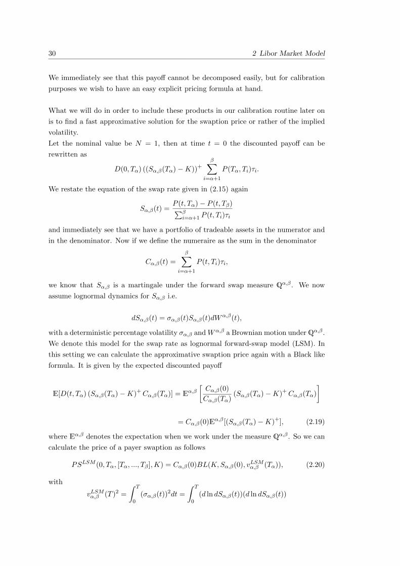
30 2 Libor Market Model
We immediately see that this payoff cannot be decomposed easily, but for calibration
purposes we wish to have an easy explicit pricing formula at hand.
What we will do in order to include these products in our calibration routine later on
is to find a fast approximative solution for the swaption price or rather of the implied
volatility.
Let the nominal value be N = 1, then at time t = 0 the discounted payoff can be
rewritten as
D(0, Tα) ((Sα,β(Tα)−K))+β∑
i=α+1
P (Tα, Ti)τi.
We restate the equation of the swap rate given in (2.15) again
Sα,β(t) =P (t, Tα)− P (t, Tβ)∑β
i=α+1 P (t, Ti)τi
and immediately see that we have a portfolio of tradeable assets in the numerator and
in the denominator. Now if we define the numeraire as the sum in the denominator
Cα,β(t) =
β∑i=α+1
P (t, Ti)τi,
we know that Sα,β is a martingale under the forward swap measure Qα,β. We now
assume lognormal dynamics for Sα,β i.e.
dSα,β(t) = σα,β(t)Sα,β(t)dWα,β(t),
with a deterministic percentage volatility σα,β andWα,β a Brownian motion underQα,β.
We denote this model for the swap rate as lognormal forward-swap model (LSM). In
this setting we can calculate the approximative swaption price again with a Black like
formula. It is given by the expected discounted payoff
E[D(t, Tα) (Sα,β(Tα)−K)+Cα,β(Tα)] = Eα,β[Cα,β(0)
Cα,β(Tα)(Sα,β(Tα)−K)+Cα,β(Tα)
]
= Cα,β(0)Eα,β[(Sα,β(Tα)−K)+], (2.19)
where Eα,β denotes the expectation when we work under the measure Qα,β. So we can
calculate the price of a payer swaption as follows
PSLSM (0, Tα, [Tα, ..., Tβ],K) = Cα,β(0)BL(K,Sα,β(0), vLSMα,β (Tα)), (2.20)
with
vLSMα,β (T )2 =
∫ T
0(σα,β(t))2dt =
∫ T
0(d ln dSα,β(t))(d ln dSα,β(t))
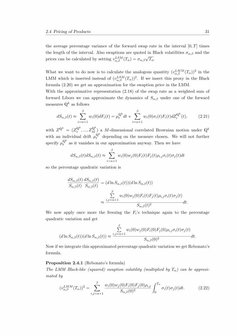
2.4 Pricing of Products 31
the average percentage variance of the forward swap rate in the interval [0, T ] times
the length of the interval. Also swaptions are quoted in Black volatilities σα,β and the
prices can be calculated by setting vLSMα,β (Tα) = σα,β√Tα.
What we want to do now is to calculate the analogous quantity (vLMMα,β (Tα))2 in the
LMM which is inserted instead of (vLSMα,β (Tα))2. If we insert this proxy in the Black
formula (2.20) we get an approximation for the swaption price in the LMM.
With the approximative representation (2.18) of the swap rate as a weighted sum of
forward Libors we can approximate the dynamics of Sα,β under one of the forward
measures Qk as follows
dSα,β(t) ≈β∑
i=α+1
wi(0)dFi(t) = µQk
t dt+
β∑i=α+1
wi(0)σi(t)Fi(t)dZQk
i (t), (2.21)
with ZQk
= (ZQk
1 , ..., ZQk
M ) a M -dimensional correlated Brownian motion under Qk
with an individual drift µQk
t depending on the measure chosen. We will not further
specify µQk
t as it vanishes in our approximation anyway. Then we have
dSα,β(t)dSα,β(t) ≈β∑
i=α+1
wi(0)wj(0)Fi(t)Fj(t)ρi,jσi(t)σj(t)dt
so the percentage quadratic variation is
dSα,β(t)
Sα,β(t)
dSα,β(t)
Sα,β(t)= (d lnSα,β(t))(d lnSα,β(t))
≈
β∑i,j=α+1
wi(0)wj(0)Fi(t)Fj(t)ρi,jσi(t)σj(t)
Sα,β(t)2dt.
We now apply once more the freezing the Fi’s technique again to the percentage
quadratic variation and get
(d lnSα,β(t))(d lnSα,β(t)) ≈
β∑i,j=α+1
wi(0)wj(0)Fi(0)Fj(0)ρi,jσi(t)σj(t)
Sα,β(0)2dt.
Now if we integrate this approximated percentage quadratic variation we get Rebonato’s
formula.
Proposition 2.4.1 (Rebonato’s formula)
The LMM Black-like (squared) swaption volatility (multiplied by Tα) can be approxi-
mated by
(vLMMα,β (Tα))2 =
β∑i,j=α+1
wi(0)wj(0)Fi(0)Fj(0)ρi,jSα,β(0)2
∫ Tα
0σi(t)σj(t)dt. (2.22)

32 2 Libor Market Model
Remark 2.4.2
In the time homogeneous case this formula has to be adjusted and looks as follows
(vLMMα,β (Tα))2 =
β∑i,j=α+1
wi(0)wj(0)Fi(0)Fj(0)
Sα,β(0)2
∫ Tα
0ρi,j(t)σi(t)σj(t)dt
=
β∑i,j=α+1
wi(0)wj(0)Fi(0)Fj(0)
Sα,β(0)2
α∑k=0
ρki,j
∫ Tk
Tk−1
σi(t)σj(t)dt.
As already stated above inserting this approximation of the swaption volatility in (2.20)
we get an approximation for the swaption price in the LMM.
If we do not freeze the drifts at the beginning for the weights wi for i = α+ 1, ..., β we
can get another more sophisticated approximation. In this case
dSα,β(t) = µQk
t dt+
β∑i=α+1
(wi(t)dFi(t) + Fi(t)dwi(t))
= µQk
t dt+
β∑i,h=α+1
(wh(t)δh,i + Fi(t)
∂wi(t)
∂Fh
)dFh(t),
where δi,i = 1, δi,h = 0 for all i 6= h and ∂wi(t)∂Fh
can be calculate as follows
∂wi(t)
∂Fh=
wi(t)τh1 + τhFh(t)
β∑k=h
τk∏kj=α+1
11+τjFj(t)
β∑k=α+1
τk∏kj=α+1
11+τjFj(t)
− 1i≥h
.Now if we set
wh(t) = wh(t) +
β∑i=α+1
Fi(t)∂wi(t)
∂Fh
we get similarly to the upper case the dynamics of the swap rate as
dSα,β(t) = µQk
t dt+
β∑i=α+1
wi(t)dFi(t).
Now we again freeze all the forward rates to get
dSα,β(t) ≈ µQk
t dt+
β∑i=α+1
wi(0)dFi(t).
So we are now in the same situation as above, see (2.21). Integration of the percentage
volatility yields Hull and White’s formula.

2.4 Pricing of Products 33
Proposition 2.4.3 (Hull and White’s formula)
The LMM Black-like (squared) swaption volatility (multiplied by Tα) can be better ap-
proximated by
(vLMMα,β (Tα))2 =
β∑i,j=α+1
wi(0)wj(0)Fi(0)Fj(0)ρi,jSα,β(0)2
∫ Tα
0σi(t)σj(t)dt. (2.23)
As the difference between the two approximations (2.22) and (2.23) is extremely small
in practice, we will use Rebonato’s formula (2.22) in our computations.
2.4.3 CMS Spread Options
A constant maturity swap spread option or short CMS spread option gives the holder
the right but not the obligation to receive the spread between two different swap rates.
Usually the swap rates on which the CMS spread option is based on are a long-maturity
and a short-maturity swap rate.23 The CMS spread option fixes both swaps at the same
fixing time Tα and pays at time Tα or Tα+1. Tβ denotes the last payment date of the
short-maturity swap and by Tγ the last payment date of the long-maturity swap, with
0 = T−1 ≤ Tα < Tβ < Tγ then the payoff looks as follows
[w(Sα,γ(Tα)− Sα,β(Tα))− wX]+,
where X denotes the option’s strike with a factor w deciding if we have a call option
(w = 1) or a put option (w = −1). In the following we will look at call options, i.e.
w = 1.
So we immediately see that these products are not sensitive to changes of the overall
level of interest rates but rather the slope of the zero-coupon curve. The value of such
a call is then given by the help of risk neutral pricing as follows
P (0, Tα)Eα[Sα,γ(Tα)− Sα,β(Tα)−X]+.
We assume that under Qα,x we have
dSα,x(t) = σα,x(t)Sα,x(t)dZα,x(t), x ∈ β, γ.
Actually we set
σ2α,x =
1
Tα
∫ Tα
0σ2α,x(t)dt, for x ∈ β, γ (2.24)
and assume
dSα,x(t) = σα,xSα,x(t)dZα,x(t), x ∈ β, γ,23By long-maturity swap rate we mean swap rates from ten years on and short-maturity swap rates
like one or two years ones. Especially the CMS spread options giving the right to exchange the ten
and two years swap rates are traded liquidly.

34 2 Libor Market Model
with Zα,x(t) Brownian motion under Qα,x.
Under Qα we have
dSα,β(t) = µα,β(t)Sα,β(t)dt+ σα,β(t)Sα,β(t)dZβ(t)
dSα,γ(t) = µα,γ(t)Sα,γ(t)dt+ σα,γ(t)Sα,γ(t)dZγ(t),
with dZβ(t) and dZγ(t) two correlated Brownian motions underQα where dZβ(t)dZγ(t) =
ρdt and the drifts are given by 24
µα,β(t) =
∑βh,k=α+1mh,k(t)τhτkFPh(t)FPk(t)ρh,kσh(t)σk(t)Fh(t)Fk(t)
1− FP (t, Tα, Tβ),
with
mh,k(t) =
[FP (t, Tα, Tβ)
∑h−1i=α+1 τiFP (t, Tα, Ti) +
∑βi=h τiFP (t, Tα, Ti)
](∑β
i=α+1 τiFP (t, Tα, Ti))2
β∑i=k
τiFPi(t),
with FPk(t) := FP (t, Tα, Tk). Note that µα,γ(t) can be calculated the same way.
We use (2.24) and apply the classical freezing the drift technique defining µα,x(t) ≈µx := µα,x(0). Then we finally get the desired joint lognormal distribution
dSα,β(t) ≈ µβSα,β(t)dt+ σα,βSα,β(t)dZβ(t),
dSα,γ(t) ≈ µγSα,γ(t)dt+ σα,γSα,γ(t)dZγ(t).
With this approximation at hand we can derive an analytical approximation for the
Libor market model price of a CMS spread option.
Proposition 2.4.4
The time t = 0 approximative price of a CMS spread option with maturity Tα > 0,
where the underlying swaps have the respective tenors (Tβ − Tα) and (Tγ − Tα), in the
Libor market model is given by
CMSSO(0, Tα) := CMSSO(0, Tα, X;β, γ) = P (0, Tα)
∫ +∞
−∞
1√2πe−
12v2f(v)dv,
(2.25)
with
f(v) =Sα,γ(0) exp[µγTα −1
2ρ2σ2
α,γTα + ρσα,γ√Tαv]
· Φ
lnSα,γ(0)h(v) + [µγ + (1
2 − ρ2)σ2
α,γ ]Tα + ρσα,γ√Tαv
σα,γ√Tα√
1− ρ2
− h(v)Φ
lnSα,γ(0)h(v) + [µγ − 1
2σ2α,γ ]Tα + ρσα,γ
√Tαv
σα,γ√Tα√
1− ρ2
24See Brigo and Mercurio [BM06] equation (6.39).

2.4 Pricing of Products 35
and
h(v) = X + Sα,β(0)e(µβ− 12σ2α,β)Tα+σα,β
√Tαv.
Proof. The proof of this proposition is an easy application of Margrabe’s formula and
can be found in Brigo and Mercurio [BM06] Appendix E.25
In Brigo and Mercurio [BM06] the authors state that we can estimate the correlation
parameter ρ historically. If we want to use the formula for model calibration we use
the following approximation.
We approximate the correlation as follows
ρ =
∫ Tα0 σα,β(t)σα,γ(t)ρβ,γ(t)dt√∫ Tα
0 σα,β(t)2dt√∫ Tα
0 σα,γ(t)2dt,
with ρβ,γ(t) denoting the instantaneous correlation between the swaprates, which can
be calculated by making use of the approximations in Section 2.4.2.
2.4.4 Bermudan Swaptions
Remember the payoff of a swaption at time Tα can be written as follows
A(Tα) = A(Tα, F (Tα);K,N) := N(
β∑i=α+1
P (Tα, Ti)τi(Fi(Tα)−K))+
and define F (t) = (Fα+1(t), ..., Fβ(t)). Therefore the time t = 0 value of the swaption
is given by
V LMMswapt (0, F (0);K,N) = P (0, Tα)Eα[A(Tα)].
A Bermudan swaption is the same as an ordinary swaption except that we can enter
the swap at the reset dates Tk, with k = α, ..., β − 1. We denote these exercise times
by T = Tα, ..., Tβ−1. So provided we have not exercised the option before, at any of
these times Tk the holder has the right to receive
A(Tk) = N(
β∑i=k+1
P (Tk, Ti)τi(Fi(Tk)−K))+.
For pricing purposes we have to fix a measure; we will choose the terminal measure, i.e.
we use P (., Tβ) as numeraire. The time t = 0 value of the Bermudan swaption under
the measure Qβ is given as follows
V LMMberm (0, F ;K,N) = P (0, Tβ) sup
τ∈TEβ[
A(τ)
P (τ, Tβ)
],
25The formula prices general exchange options under the assumption of a joint lognormal distribution
for the underlyings and was introduced in Margrabe [Mar78].

36 2 Libor Market Model
where τ ∈ T denotes the exercise time. Now if we want to price that Bermudan
swaption by means of Monte Carlo we would step forward in time and we would face
the problem of having to do a recursive Monte Carlo algorithm. To calculate the time
Tk value of the Bermudan swaption we have to calculate the value of A(Tk) and the
value if we hold it and exercise it later on denoted by C(Tk, F (Tk)). The problem is
that the calculation of the holding value C(Tk, F (Tk)) involves all A(Ti) for all Ti ∈ T ,
where Ti > Tk. This holding value can be calculated by an additional Monte Carlo
simulation but this straightforward approach, although it works, is very slow. But
there are more advanced techniques, one possibility is for example to use Monte Carlo
combined with backward oriented methods, which we will describe briefly below.
Regression-Based Monte Carlo Method
A popular representative of these regression-based algorithms is the well-known Longstaff-
Schwarz algorithm. In the following we will give a brief introduction how to calculate
the price of a Bermudan swaption in a Libor market model. For further details see
Brigo and Mercurio [BM06], Glasserman [Gla04] and Longstaff and Schwartz [LS01],
furthermore Hippler gives a good overview in [Hip08].
For notational convenience we will from now on denote the time t value of the Bermudan
swaption by
V (t, F (t)) := V LMMberm (t, F ;K,N).
At time Ti ∈ T the holder has to decide whether to continue to hold the option or to
exercise it immediately. The holding value can be expressed as
C(Ti, F (Ti)) := P (Ti, Ti+1)E[V (Ti+1, F (Ti+1))|F (Ti)],
so the value of the Bermudan swaption V (Ti, F (Ti)) can be expressed via the following
dynamic programming recursion
V (Tβ−1, F (Tβ−1)) = P (Tβ−1, Tβ)Nτβ(Fβ(Tβ−1)−K)+,
V (Tj , F (Tj)) = max[A(Tj), C(Tj , F (Tj))],
for j = i, ...., β− 2. We start at time Tβ−1 until we reach time Ti. If we knew the value
of C(Tj , F (Tj)) we might also use it in a forward instead of a backward way. We would
just exercise it, if A(Ti) > C(Ti, F (Ti)) and otherwise we would hold the option. This
is also the link between the forward fashion Monte Carlo method and the backward
oriented method.
We will now introduce a method of approximating the continuation value by means of

2.5 Calibration 37
a regression-based approach in the following lines.
We simulate np paths of the underlying forward Libor rates and get the tuples
(F k(Ti), Pk(Ti, Ti+1)V (Ti+1, F
k(Ti+1))), k = 1, ..., np, ∀i = α, ..., β − 1.
Then we select mi basis functions, i.e. φj,i(.), j = 1, ...,mi, for each possible exercise
time Ti, obvious candidates in our setting are functions of the forward rates F (Ti), for
example the swap rate, the square and the cubic swap rate. Then we try to find the
weights λl,i such that the continuation value is approximated as good as possible, i.e.
C(Ti, F (Ti)) ≈ C(Ti, F (Ti)) :=
mi∑l=1
λl,iφl,i(F (Ti)),
by means of a least-squares estimation with the set of the tuples from above. So after
we obtained the weights we have a possibility to approximate the holding value at every
exercise time and therefore we are able to calculate the price of the Bermudan option
without the need to perform an additional Monte Carlo simulation for the holding
value.
2.5 Calibration
To calibrate the model to market data we have to provide the initial Libor forward
rates, the respective Black volatilities for the caplets and swaptions and finally, de-
pending on the preferences, the historically estimated correlation matrix or the prices
of the CMS spread options.
The initial Libor rates are only available up to one year and therefore have to be stripped
from other traded products. This will be done in the following subsection. After that
we devote Subsection 2.5.2 to the caplet volatilities, which have to be stripped from cap
prices. The swaption volatilities and the CMS spread option prices are directly quoted
in the market. To estimate the historical correlation matrix we have to build a yield
curve for a whole history of dates and then calculate the correlations from this series
of yield curves. In the subsequent Subsections 2.5.3 - 2.5.5 we show how to include
each of these products in a calibration routine. The last section deals with the task of
choosing products for the calibration depending on the product we wish to price with
the model.
We denote the vector of time inhomogeneity parameters Φ and the vector of correlation
parameters ρ as
Φ = [Φ1, ...,ΦM ] and ρ = [ρ1, ..., ρc],
where the number of correlation parameters denoted by c depends on the chosen
parametrization.

38 2 Libor Market Model
2.5.1 Stripping of the Forward Interest Rate Curve
The first question we have to ask is where do we get the initial values for the forward
Libor rates from. From the British Bankers’ Association (BBA) we can get Libor rates
for overnight rates, weekly data, two weekly data and monthly data ranging from one
to twelve months.26 So the longest rate is a twelve months Libor rate, but we need
a much longer term structure. To strip a whole forward curve we will use a mix of
products consisting of depot rates ranging from overnight up to one year, FRAs or
futures for one to about two years and swaps for the maturities from two to 50 years.
The forward curve can then be stripped by a straightforward bootstrapping algorithm
as described for example in the lecture notes of Lesniewski and Andersen [LA07]. From
the products we calculate the corresponding discount rates P (0, T ) and therefore get a
grid of discount factors from which we can then calculate the forward rates via
F (0, Ti−1, Ti) = τi
(P (0, Ti−1)
P (0, Ti)− 1
).
To calculate the whole forward curve we will need some discount factors which are not
on the stripped grid and therefore we have to choose an interpolation method between
the stripped rates. We can use linear, log-linear or spline interpolation just to mention
a few. Furthermore we have to be careful about the respective daycount and business
day conventions of the products. For example we have to use Actual/360 for the deposit
cash positions. For futures and FRA’s we also have to use Actual/360. The 30/360
daycount convention is used for the fixed leg of a swap and in case of a Libor/Euro
market swap we use Actual/360 for the floating leg.27
The last thing we have to specify is a holiday calender in our case we choose the TAR-
GET calender.
To omit implementing all the calenders and business day conventions from the scratch
we use the implementation provided by Quantlib for our calibrations.
We will now outline the main ideas of the stripping algorithm. We suppose we have
a tenor τ , for example six months, for our forward rates, i.e. we work on a grid with
Ti = Ti−1 + τ for i = 1, ...,M and T0 = τ . Then we first have to get the discount
factors on this grid by making sure that the given products yield the correct values and
then interpolate and extrapolate the values for the other necessary discount factors.
We start with the product with the shortest maturity and make our way through to
the product with the longest maturity.
26This data is freely available from http://www.bbalibor.com.27See for example Zagst [Zag02].

2.5 Calibration 39
Then we calculate the values of the forward rates as
Fi(0) = F (0, Ti−1, Ti) = τ
(P (0, Ti−1)
P (0, Ti)− 1
), ∀i = 1, ...,M.
2.5.2 Volatilities and Correlations
Before we start discussing the calibration, we fix the parametric form of the volatility.
We will from now on use the parametrization given by (2.4)
σi(t) = Φiψ(Ti−1 − t; a, b, c, d) := Φi
([a+ b(Ti−1 − t)]e−c(Ti−1−t) + d
).
For the moment we will not fix the parametrization for the correlation.
For the correlation we have two different approaches for the calibration:
• The endogenous (implied) method, where we find the correlations by calibrating
correlation sensitive products like swaptions or even better CMS spread options.
• The exogenous (historical) method, where we fit the correlation parametrization
to the empirically observed correlations between the forward rates.
We think that it makes more sense to use the implied method to stay consistent as we
also use implied volatilities. On the other hand when we change the measure from real
world to the risk neutral one, Girsanov’s theorem makes sure the correlations stay the
same so there should not be a difference. If we use historical correlations we have the
usual problems connected with historical data: outliers, non-smooth correlation sur-
faces, holes in the data, different choices of the considered data and the interpolation
scheme. In Brigo and Mercurio [BM06] we find many possibilities how to tackle the
fitting of the parametrized correlation matrix to historical data. At this point we only
want to mention again that we found some stability problems regarding the pivot meth-
ods, especially when we have data sets that show irregularities. Therefore we rather
suggest to use the best fit approaches, if we wish to calibrate the model to historical
correlations.
What we suggest to do is to include the correlation parameters in our calibration. As
we stated earlier caplets are not influenced at all by correlation. In the case of swaptions
we have the problem that different volatility structures imply decorrelation indepen-
dent of the correlation.28 Swaptions are sensitive to terminal correlation and do not
rely on the instantaneous correlation directly, therefore it is hard to strip correlation
information from swaption quotes. So to get reliable information we need to include
a liquidly traded product which heavily depends on correlation and admits a, at least
28The phenomena of decorrelation is described in Section 2.3.5.

40 2 Libor Market Model
approximatively, closed-form solution. Such a product is the CMS spread option intro-
duced in Section 2.4.3. The paper of Van Heys and Borger [VHB09] is devoted to this
problem.
If we do not have an (approximative) closed-form solution at hand, as it is the case for
callable products like the Bermudan swaptions, which we introduced in Section 2.4.4,
we need to resort to Monte Carlo methods for pricing these products, which is in most
cases much too slow to be used in a calibration routine.
2.5.3 Caplet Calibration
The first thing we want to do is calibrate the model to caplet prices. The problem we
face is that in the market we only find quoted cap prices, so the first step will be to
strip caplet prices from them. As we know from (2.12) cap prices29 are just a sum of
individual caplets and there are some straightforward easy bootstrapping algorithms
to strip the caplet volatilities readily available.30 In our numerics part we use the very
robust implementation provided by Quantlib.
In case of caplets we have a one-to-one correspondence between option prices and
implied volatilities, which means that it does not matter if we have the implied volatility
or the price of the caplet at hand. To get the price we just insert the implied volatility
σMkti in the Black Scholes formula, i.e.
CapletMktTi = NP (0, Ti)τiBL(K,Fi(0), σMkt
i
√Ti−1).
On the other hand if we have the price given we just invert the formula and get the
implied volatility. So the implied volatility is just another way of quoting the price
and it is the way data providers do provide us with market quotes. Therefore we can
fit the volatilities provided by the parametrization directly to the quoted or rather
stripped caplet volatilities. Therefore for calibration purposes there is no need of a
pricing formula for the caplets.
We set for a moment Φ = (1, ..., 1) and define
vk(a, b, c, d) =√v2k(a, b, c, d) :=
√∫ Tk−1
0σk(a, b, c, d; t)2dt
is the square root of the integrated variance, where we used the notation σk(a, b, c, d; t)
to stress the dependence of the volatility function on the volatility parameters. Fur-
thermore we define the implied volatilities from the model as follows
σk(a, b, c, d) :=1√Tk−1
vk(a, b, c, d),
29To be precise the Black volatilities are quoted.30For more details on the stripping algorithm see Brigo and Mercurio [BM06].

2.5 Calibration 41
for all k = 1, ...,M . The optimization then looks as follows
min(a,b,c,d)
[K∑k=1
wkg(σMktik
, σik(a, b, c, d))
], (2.26)
where K denotes the number of caplets that we calibrate the model to, wk are some
weights used to control the closeness of the model to the specific caplet and ik ∈1, ...,M for all k = 1, ...,K. Furthermore the distance function g must be chosen
depending on what we want to minimize. If we want to minimize the squared absolute
error between the volatilities we might choose for example g(x, y) = (x − y)2, or the
squared relative error by using g(x, y) = (x−y)2
x2 , which is the function we suggest to
use. If we want to minimize the price difference we will have to calculate the prices
first by inserting the volatilities in the Black formula. We stress here that we may
use any strikes for the caplets,31 but usually one uses at the money (ATM) caplets.
Depending on the product we want to price we may also use other strikes, but we can
only calibrate it to one strike per maturity at a time, i.e. we cannot calibrate it to
two caplets with the same maturity and two different strikes, because the Libor market
model has no smile features due to the lognormal dynamics. Therefore if we wish to
include skew or smile information we have to extend the Libor market model, which
will be the topic of Chapters 3 and 4. As we stated above it would not make any sense
to include correlation parameters in this calibration as these products are not sensitive
to correlation. If we want to calibrate the model to caplet prices we would have to fit
the correlation parameters to historical correlations or we can use swaptions and CMS
spread options to include information on correlation. In our tests we fitted the a, b, c, d
parameters to the ATM caplet volatility surface and observed that the fit we can obtain
is usually quite good.
By making use of the previously defined Φi’s we can fit all caplets CapletTi perfectly
by calibrating the Φi’s for i = 1, ...,M , no matter what the parameters a, b, c and d
look like.
Actually there are two ways to calibrate the Φi’s:
• Calibrate the abcd parameters via (2.26) and choose the Φi’s as
Φ2i =
Ti−1(σMkti )2
v2i (a, b, c, d)
, ∀i = 1, ...,M.
In this case we have four parameters to calibrate and get the other M parameters
automatically, but the model is not time homogeneous anymore.
• Or calibrate them directly with the other parameters and include a penalty func-
tion to penalize the deviation from the time homogeneity paradigm. In this case
31As long as we also use the same strikes for the market and the model volatility.

42 2 Libor Market Model
M + 4 parameters have to be calibrated.32
To obtain meaningful parameters we should have K ≥M +4, or if we set Φi = 1 for all
1 ≤ i ≤M , we should make sure that K ≥ 4. An easy example for a penalty function
would be fp(Φi) = p · (1 − Φi)2, where p is a penalty factor, which can be chosen by
the user of the model. The optimization then looks as follows
min(a,b,c,d,Φ)
K∑k=1
wkg(σMktik
, σik(a, b, c, d,Φk)) +M∑j=1
fp(Φj)
. (2.27)
Furthermore we have to think about how to include the constraints for the parameters.
We suggest to add a penalty function when the bounds are violated, e.g. if parameter
x is smaller than the lower bound xlb we add exp(γ(xlb − x)) with some factor γ > 0.
2.5.4 Swaption Calibration
In Section 2.4.2 we stated two approximative formulas for swaption volatilities in the
Libor market model, namely Rebonato’s Formula (2.22) and Hull and White’s Formula
(2.23), which can be used in a similar fashion as in the caplet case. The market also
quotes swaption prices as implied volatilities which need to be inserted in the Black
like Formula (2.20) to obtain the actual market prices. We will also try to get the
approximative swaption volatilities as close as possible to the observed market quotes.
In the following we will use Rebonato’s Formula (2.22) given as
(vLMMα,β (Tα))2 =
β∑i,j=α+1
wi(0)wj(0)Fi(0)Fj(0)ρi,jSα,β(0)2
∫ Tα
0σi(t)σj(t)dt.
We define
σα,β :=
√1
Tα(vLMMα,β (Tα))2
and we will use later the notation σα,β(a, b, c, d, ρ) = σα,β to stress that it is the volatility
coming from a model with parameters a, b, c, d and ρ. σMktα,β denotes the swaption
volatility quoted by the market.
We immediately see that in this case the instantaneous correlation is included in the
formula. So we need to fit the a, b, c, d parameters to get the correct σk’s and the
correlation parameters to get the correct instanteneous correlation. We already stated
before that different parameter combinations for a, b, c, d may yield similar values for
the vk’s. This means they yield the same caplet prices, but may introduce different
levels of decorrelation and therefore we can get equally good fits to the caplet prices
and swaption prices with different a, b, c, d parameters and different parameters for
the instantaneous correlations. So we do not know whether the decorrelation comes
32Note that in this case the fit will not be perfect in general anymore.

2.5 Calibration 43
from the volatilities or the instantaneous correlation making it hard to obtain robust
correlation parameters. A joint calibration to caplets and swaptions then looks as
follows:
• If we set Φ = (1, ..., 1)
min(a,b,c,d,ρ)
[ K∑k=1
wCk g(σMktik
, σik(a, b, c, d)) (2.28)
+
J∑j=1
wSj h(σMktαj ,βj
, σαj ,βj (a, b, c, d, ρ))
],
with αj , βj ∈ 1, ...,M. J denotes the number of swaptions we use for the
calibration and h is a function similar to g. wC = (wC1 , ..., wCK) and wS(wS1 , ..., w
SJ )
denote the individual weight vectors for the caplets and swaptions respectively.
In order to get meaningful parameters we must make sure that we calibrate the
model to at least 4 + c products, i.e. K + J ≥ 4 + c.
• The Φ’s can again be used to fit the caplets perfectly, but in this case we would
introduce an additional error for the swaption volatilities.
• We might also calibrate the abcd parameters to the caplets use the Φ’s to get a
perfect fit and then find the perfect vector ρ to fit the swaptions, i.e. we do a two
step calibration
min(a,b,c,d)
[ K∑k=1
wCk g(σMktik
, σik(a, b, c, d))
], (2.29)
minρ
[ J∑j=1
wSj h(σMktαj ,βj
, σαj ,βj (ρ))
]. (2.30)
We do not suggest this very fast optimization as we will not get the global opti-
mum in this case.
• Or we also calibrate the Φi’s by the help of a penalty function fp : R 7→ R+ as
follows
min(a,b,c,d,Φ,ρ)
[ K∑k=1
wCk g(σMktik
, σik(a, b, c, d,Φk)) (2.31)
+J∑j=1
wSj h(σMktαj ,βj
, σαj ,βj (a, b, c, d, Φ, ρ)) +M∑m=1
fp(Φm)
].
Again we have to make sure that K + J ≥ M + 4 + c to obtain meaningful
parameters.

44 2 Libor Market Model
2.5.5 CMS Spread Option Calibration
In the same fashion we can include the correlation sensitive CMS spread options. We
again need to calibrate the model parameters as close as possible to the market prices
by the help of the approximative Formula (2.25). Similarly to including swaptions we
get
min(a,b,c,d,ρ)
[ K∑k=1
wCk g(σMktik
, σik(a, b, c, d)) (2.32)
+
J∑j=1
wSj h(σMktαj ,βj
, σαj ,βj (ρ))
+L∑l=1
wCMSSOl r(CMSSOMkt
l , CMSSOl(a, b, c, d, ρ))
],
where r is a function similar to g and h. wCMSSO = (wCMSSO1 , ..., wCMSSO
L ) denotes
the individual weight vector for the CMS spread options and CMSSOl(a, b, c, d, ρ) de-
notes the price of the CMS spread option we wish to calibrate.
In both cases we may fit the caplets perfectly after the optimization by choosing the Φ’s
as discussed above, but then we must be aware that we introduce an uncontrolled error
in the other products. Another possibility, as introduced above, would be to include
the Φ’s in the calibration with the help of a penalty function fp : R 7→ R+ with a
penalty factor p. Then the calibration looks as follows
min(a,b,c,d,Φ,ρ)
[ K∑k=1
wCk g(σMktik
, σik(a, b, c, d,Φk)) (2.33)
+J∑j=1
wSk h(σMktαj ,βj
, σαj ,βj (a, b, c, d, Φ, ρ))
+L∑l=1
wCMSSOl r(CMSSOMkt
l , CMSSOl(a, b, c, d, Φ, ρ))
+M∑k=1
f(p,Φk)
].
Another approach is to strip the terminal correlation from the market data first and
then try to fit the parameters to get the terminal correlation obtained by the model
Corr(a, b, c, d, Φ, ρ) to the market implied terminal correlations CorrMkt. In this case
we would useL∑l=1
wCMSSOl r(CorrMkt
l , Corrl(a, b, c, d, Φ, ρ)) (2.34)

2.5 Calibration 45
instead ofL∑l=1
wCMSSOl r(CMSSOMkt
l , CMSSOl(a, b, c, d, Φ, ρ))
in (2.33) with an adjusted function r.
To strip the correlations we use the CMS spread option formula (2.25) from above. If
we want to calibrate the model to an estimated historical correlation matrix we can use
the same function as in (2.34). Again we have to make sure that K+J+L ≥M+4+ c
in order to obtain meaningful parameters.
2.5.6 Choosing Products for the Calibration
The optimal choice of the weights depends heavily on the product which we intend to
price. Furthermore we have to think about hedging in this context. If we want to hedge
a product we should try to find parameters such that the products used for hedging
are fitted well.
Digital Caplet
This is a pathological case because setting up a LMM for a digital caplet is like shooting
sparrows with cannons. For the digital caplet with strike K and maturity Tj the only
information that is really interesting is the caplet volatility of the caplets maturing at
the same maturity as the digital caplet we want to price. We immediately see that no
correlation information is used and therefore it makes no sense to include swaptions
and CMS spread options in the calibration. So we would choose the caplets with strikes
K and for the weights wj = 1 and wi = 0, ∀i 6= j, where wj denotes the weight of the
caplet maturing at Tj . Furthermore we would have to add artificially some products
to the calibration to get good results as we need at least as many prices as we have
parameters to calibrate.
Bermudan Swaption
If we want to price an exotic product like a Bermudan swaption it actually makes sense
to use a well calibrated Libor market model. To get an overall good fit to the observed
volatility structure we might calibrate at the money (ATM) caplets. Then we might
wish to catch the correlation matrix as good as possible and therefore include CMS
spread options. Now we have to think about which swaptions to include. We know
that the Bermudan swaption is something like a collection of co-terminal swaptions so
we will have to calibrate the model especially well to these underlying co-terminals.

46 2 Libor Market Model
Range Accruals
This product heavily depends on the value at its range borders. Lets assume we have a
range accrual paying a Libor rate as long as it stays in between three and five percents.
If we forget about the correlation for a moment the task comes down to fitting the
caplets with strikes at three and five percents as good as possible. The LMM is only
capable of fitting one of these caplet series well, as it cannot include the given market
skew or smile. In this case we might calibrate it to the four percent strike level and
hope that the errors will not be too dramatic. What we really suggest is to include
the market skew or better the market smile by using more sophisticated Libor market
models. This will be the topic of the next two chapters.

3 Displaced Diffusion Libor Market Model
There are many possibilities to model the skew, for example a CEV, or a lognormal
mixture model. We will concentrate on the displaced diffusion setting as the dynamics
specified by a displaced diffusion are very similar to the dynamics coming from a CEV
model,1 but we have much easier Black like formulas for the evaluation of the products
used for calibration. For an overview of different possibilities to include the skew in a
Libor market model see Brigo and Mercurio [BM06]. In the next chapter we will deal
with stochastic volatility extensions to include the market smile. The model we will
actually choose is a displaced diffusion model with stochastic volatility. Therefore we
now have a look at different versions of displaced diffusion Libor market models and
compare their features. At the end of this chapter we have a short look at the pricing
and calibration issues but we will not go into details for these models as we concentrate
mainly on the stochastic volatility extension in this thesis.
3.1 Modeling of Forward Libor Rates
We again denote by Fk the forward Libor rate ranging from Tk−1 to Tk with k = 1, ...,M
and 0 = T−1 < T0 < T1 < · · · < TM . Now we do not model the M forward rates as
a lognormal random variables under their respective forward measures, but we rather
suppose that the dynamics of each forward Libor rate Fk under its specific forward
measure Qk (i.e. numeraire P (0, Tk) ) look as follows
dFk(t) = φk(Fk(t), t)σk(t)dWk(t), k = 1, ...,M,
with a M -dimensional correlated Brownian motion under Qk and some function φk
that has to be specified. If we choose φk(x, t) = x we are back in the ordinary Libor
market model from Chapter 2.
If we look at all forward Libors under one measure Qi the we get
• i = k, t ≤ Tk−1 :dFk(t)
φk(Fk(t), t)= σk(t)dWk(t)
• i < k, t ≤ Ti :
dFk(t)
φk(Fk(t), t)= σk(t)
k∑j=i+1
ρk,j(t)τjσj(t)φj(Fj(t), t)
1 + τjFj(t)dt+ σk(t)dWk(t)
1More details on how close these models are to each other can be found in Muck [Muc03].

48 3 Displaced Diffusion Libor Market Model
• i > k, t ≤ Tk−1 :
dFk(t)
φk(Fk(t), t)= −σk(t)
i∑j=k+1
ρk,j(t)τjσj(t)φj(Fj(t), t)
1 + τjFj(t)dt+ σk(t)dWk(t)
whereW is aM -dimensional correlated Brownian motion underQi with dWi(t)dWj(t) =
ρi,j(t)dt for all i, j = 1, ...,M .
There is a variety of functions φk(Fk(t), t) which might be used to model the Libor
rates.
Remark 3.1.1
Some examples for the function φk(x, t) are
• φk(x, t) = x (LMM)
• φk(x, t) = x+ bk(t) (displaced diffusion LMM)
• φk(x, t) = ak(t)x+ bk(t) (displaced diffusion LMM version used by Piterbarg)
• φk(x, t) = xα (CEV LMM)
From Muck [Muc03] we know that we can generate very similar dynamics by a displaced
diffusion and a CEV model. But as we have much easier formulas for the caplet prices
in a displaced diffusion setting we will rather use the displaced Libor market model.
Our focus will be on the following time independent
φk(Fk(t), t) = Fk(t) + bk and φk(Fk(t), t) = akFk(t) + bk, (3.1)
and time dependent choices
φk(Fk(t), t) = Fk(t) + bk(t) and φk(Fk(t), t) = ak(t)Fk(t) + bk(t). (3.2)
Time Independent Displaced Diffusion LMM
The modeling approach we will introduce here is a standard approach taken by many
researchers and practitioners, see for example Joshi and Rebonato [JR03].2 If we use
the function φ(Fk(t), t) = Fk(t)+bk for each k = 1, ...,M we get the following dynamics
dFk(t) = d(Fk(t) + bk) = (Fk(t) + bk)σk(t)dWk(t), k = 1, ...,M,
where W is a M -dimensional correlated Brownian motion under Qk, a deterministic
displacement factor bk and σk a deterministic volatility function similar to the ordinary
LMM.2The first who used displaced diffusion for modeling was Rubinstein [Rub83].

3.1 Modeling of Forward Libor Rates 49
Under an arbitrary forward measure Qi we have for example for i < k, t ≤ Ti :
dFk(t) = σk(t)(Fk(t) + bk)k∑
j=i+1
ρk,j(t)τjσj(t)(Fj(t) + bj)
1 + τjFj(t)dt+ σk(t)(Fk(t) + bk)dWk(t),
where W is a M -dimensional correlated Brownian motion under Qi. The same can be
derived for the other functions stated in Remark 3.1.1.
Time Dependent Displaced Diffusion LMM
We can introduce time dependence in the displacements by choosing φk(Fk(t), t) =
Fk(t) + bk(t) for each k = 1, ...,M , which yields the following dynamics under the
forward measure Qk
dFk(t) = (Fk(t) + bk(t))σk(t)dWk(t).
Another very appealing modeling approach is given as follows.3 If we choose φk(Fk(t), t) =
ak(t)Fk(t) + (1− ak(t))Fk(0) for each k = 1, ...,M , we get
dFk(t) = [ak(t)Fk(t) + (1− ak(t))Fk(0)]σk(t)dWk(t).
Actually this is a quite clever choice because in the first model the volatility is pro-
portional to the displaced process, whereas in the second setting it is proportional to
the process itself.4 This setting makes it possible to split up the calibration problem
in a volatility/correlation calibration and a skew calibration. If we change the dis-
placement factor in the first setting it also influences the volatility, so we have to do
a joint calibration.5 In the second case the parameter does not influence the volatility
and therefore we can calibrate the parameters separately. This means that when it
comes to calibration the second approach is more stable, easier and faster to calibrate.
But as the calibration of a displaced LMM involves quite easy Black like formulas the
calibration is quite easy and fast anyway and the gains of such a splitting are not too
tremendous. Therefore it is left to the reader, which model he prefers. First when we
extend it to include stochastic volatility we really gain a lot regarding computational
time. Therefore in the stochastic volatility extension of Chapter 4 we will make use of
the second setting.
3For details See Marris [Mar99].4Actually it is only at the very first instant proportional to the swap rate itself and later to some
mixture of the starting value and the current value, but it has the same magnitude.5For more details see the next section.

50 3 Displaced Diffusion Libor Market Model
3.1.1 Equivalence of the Modeling Approaches
Time Independent Displaced Diffusion
In the following we analyse how the two approaches from above correspond to each
other.
If we assume to use the abcd parametrization stated in (2.4) we have the following
xσi(t) = x([a+ b(Ti−1 − t)]e−c(Ti−1−t) + d) = [xa+ xb(Ti−1 − t)]e−c(Ti−1−t) + xd,
so we see that if we multiply σ by some factor x it has the same effect as if we multiply
a, b and d by the factor x.
Now we look at the forward Libor Fk under its natural measure Qk. We can rewrite it
as follows
dFk(t) = (Fk(t) + bk)σbk(t)dWk(t) = (γkFk(t) + (1− γk)Fk(0))σγk (t)dWk(t),
with
bk =(1− γk)Fk(0)
γk
and
σbk(t) = γkσγk (t)
and so
ab = γkaγ , bb = γkb
γ , cb = cγ , db = γkdγ .
We see that we can directly translate the parameters from the time independent dis-
placed diffusion model to the parameters of the alternative model, which is used by
Piterbarg and which will be used by us in the numerics part. To be precise we will use
the time dependent alternative which we introduce below.
Alternative Modeling Approach (Time Dependent Displaced Diffusion)
Furthermore we can introduce time dependence in the displacements which yields the
following dynamics
dFk(t) = (Fk(t) + bk(t))σbk(t)dWk(t) = (γk(t)Fk(t) + (1− γk(t))Fk(0))σγk (t)dWk(t)
with
bk(t) =(1− γk(t))Fk(0)
γk(t)
and
σbk(t) = γk(t)σγk (t)

3.1 Modeling of Forward Libor Rates 51
and so
ab = γk(t)aγ , bb = γk(t)b
γ , cb = cγ , db = γk(t)dγ ,
here we can also see that we find equivalent parameters, but now we have time depen-
dent abcd parameters making it impossible to get a direct link between these models.
But still these models should be very close to each other leading to very similar caplet
prices.
3.1.2 Terminal Correlation
In this section we will derive an approximative formula for the time independent case.
The terminal correlation is the correlation between two forward rates, i.e.
CorrQ(Fi(T ), Fj(T )) =EQ[(Fi(T )− EQ(Fi(T )))(Fj(T )− EQ(Fj(T )))]√
EQ[(Fi(T )− EQ(Fi(T )))2]√EQ[(Fj(T )− EQ(Fj(T )))2]
=EQ[Fi(T )Fj(T )]− EQ[Fi(T )]EQ[Fj(T )]√
EQ[(Fi(T )− EQ(Fi(T )))2]√EQ[(Fj(T )− EQ(Fj(T )))2]
,
under some forward measure Q.
So we have to calculate the following quantities:
1. EQ[Fi(T )]EQ[Fj(T )]
2. EQ[Fi(T )Fj(T )]
3. EQ[(Fi(T )− EQ(Fi(T )))2]
For notational convenience we skip the Q in EQ in the following.
As a reminder we look at the dynamics of the shifted process. We denote by α = bk
d(Fk(t) + α) = d(Fk(t) + α)(µQk (t)dt+ σk(t)dWk(t)),
where the drift depends on the chosen measure and get, if we freeze the forward Libor
rates in the drifts at their time 0 values and denote them by µ0k(t), the following
Fk(T ) + α ≈ (Fk(0) + α) exp
(∫ T
0µ0k(t)−
σ2k(t)
2dt+
∫ T
0σk(t)dWk(t)
).
The first quantity can easily be calculated as follows
E[Fi(T )] = E[(Fi(T ) + α)− α] = E[(Fi(T ) + α)]− α (3.3)
and therefore
E[Fi(T )]E[Fj(T )] = E[(Fi(T )+α)]E[(Fj(T )+β)]−αE[(Fj(T )+β)]−βE[(Fi(T )+α)]+αβ,
(3.4)

52 3 Displaced Diffusion Libor Market Model
with the notation α = bi and β = bj used for convenience reasons.
We now address the second quantity
Fi(T )Fj(T ) = (Fi(T ) + α− α)(Fj(T ) + β − β)
= (Fi(T ) + α)(Fj(T ) + β)− β(Fi(T ) + α)− α(Fj(T ) + β) + αβ, (3.5)
so the expectation is given as
E[Fi(T )Fj(T )] = E[(Fi(T )+α)(Fj(T )+β)]−βE[Fi(T )+α]−αE[Fj(T )+β]+αβ. (3.6)
We can immediately see that this only depends on the displaced processes.
To get the third quantity we will need to calculate some additional quantities
E[F 2i (T )] = E[(Fi(T ) + α− α)2] = E[(Fi(T ) + α)2]− 2αE[(Fi(T ) + α)] + α2, (3.7)
E[Fi(T )]2 = E[(Fi(T ) + α)− α]2 = E[(Fi(T ) + α)]2 − 2αE[(Fi(T ) + α)] + α2, (3.8)
E[(Fi(T )− E[Fi(T )])2] = E[Fi(T )2]− 2E[Fi(T )]2 + E[Fi(T )]2 = E[Fi(T )2]− E[Fi(T )]2
(3.7), (3.8)= E[(Fi(T ) +α)2]−E[(Fi(T ) +α)]2 = E[(Fi(T ) +α)2−E[(Fi(T ) +α)]2]. (3.9)
We know that if we freeze the drifts then X := Fi(T ) + α and Y := Fj(T ) + α are
lognormally distributed and therefore we can use the same formulas as in the LMM,
see Section 2.3.5.
CorrQ(Fi(T ), Fj(T ))(3.4) , (3.6), (3.9)
=E[XY ]− E[X]E[Y ]√
E[X2]− E[X]2√E[Y 2]− E[Y ]2
≈ ρi,j
∫ T0 σi(t)σj(t)dt√∫ T
0 σ2i (t)dt
√∫ T0 σ2
j (t)dt.
3.2 Pricing of Products
3.2.1 Caplets
We have a look at the price of a caplet with nominal value N = 1 in the displaced
diffusion Libor market model. It is given as
CplDD(0, Tk−1, Tk, τk,K) = τkP (0, Tk)Ek[(Fk(Tk−1)−K)+
]= τkP (0, Tk)E
k[((Fk(Tk−1) + bk)− (K + bk))
+],

3.2 Pricing of Products 53
with our lognormal dynamics under Qk
d(Fk(t) + bk) = (Fk(t) + bk)σk(t)dWk(t),
we get
CplDD(0, Tk−1, Tk, τk,K) = τkP (0, Tk)BL(K + bk, Fk(0) + bk, Vk(Tk−1)), (3.10)
where
Vk(Tk−1) =
√∫ Tk−1
0σk(s)2ds
and
BL(K,F, v) = FΦ
(ln(F/K) + v2/2
v
)−KΦ
(ln(F/K)− v2/2
v
).
Alternative Formulation
For convenience reasons we will skip the k in Fk and its parameters. As stated in the
last section with our lognormal dynamics under Q we have
dF (t) = (γF (t) + (1− γ)F (0))σγ(t)dW (t) = (F (t) + b)σb(t)dW (t),
with
b =(1− γ)F (0)
γ
and by setting
ab = γaγ , bb = γbγ , cb = cγ , db = γdγ ,
we have
σb(t) = γσγ(t)
and we also get
Vk(Tk−1) =
√∫ Tk−1
0σbk(s)
2ds = γ
√∫ Tk−1
0σγ(s)2ds,
CplDD′(0, Tk−1, Tk, τk,K) = τkP (0, Tk)BL(K + b, F (0) + b, V (Tk−1)).
Time Dependent Case
As stated in the last section with our lognormal dynamics under Q we have
dF (t) = (γ(t)F (t) + (1− γ(t))F (0))σγ(t)dW (t) = (F (t) + b(t))σb(t)dW (t)
with
b(t) =(1− γ(t))F (0)
γ(t)

54 3 Displaced Diffusion Libor Market Model
and by setting
ab = γ(t)aγ , bb = γ(t)bγ , cb = cγ , db = γ(t)dγ ,
we have
σb(t) = γ(t)σγ(t).
So we get
V (Tk−1) =
√∫ Tk−1
0σb(s)2ds =
√∫ Tk−1
0γ2(s)σγk (s)2ds.
But here we have the problem to calculate Vk(Tk−1). In Section 4.2 we will look at the
Markovian projection technique which yields the so-called effective skew. The effective
skew is something like a time averaged parameter, which is then used instead of the
time dependent skew
γ(t) = γeff .
Then we are back in the case of the alternative formulation and we can use the formulas
from above.
Vk(Tk−1) =
√∫ Tk−1
0σb(s)2 = γeff
√∫ Tk−1
0σγ(s)2,
with
ab = γeffaγeff, bb = γeffbγ
eff, cb = cγ
eff, db = γeffdγ
eff.
3.2.2 Swaptions
For the pricing of swaptions we move to the swap measure Qα,β and suppose that the
dynamics of the swap rate is given as follows
dSα,β(t) = σα,β(t)φα,β(Sα,β(t), t)dWα,β(t),
so we are again in an ordinary displaced diffusion setting and we can use Formula (3.10)
again to calculate the price of a swaption. We only have to specify the local volatility
function φα,β. One possibility to calculate it is to make sure that
φα,β(Sα,β(t), t)σα,β(t) = φj(Fj(t), t)σj(t), ∀j = α+ 1, ..., β.
This can not be solved in general and therefore we use
φα,β(Sα,β(t), t) =
β∑j=α+1
φj(Fj(t), t)σj(t)σα,β(t)ρj,(α,β)(t)
σα,β(t)2,
where ρj,(α,β)(t) denotes the instantaneous correlation between the forward Libor rate
and the swap rate, as an approximation.6
6For details see Piterbarg [Pit03b].

3.3 Calibration 55
3.3 Calibration
We will only briefly introduce the basic ideas for the calibration because it is very
similar to the LMM calibration in Section 2.5 and therefore we want to concentrate on
the more demanding stochastic volatility model calibration in the next chapter. The
calibration is analogue to the calibration of the LMM with a slightly different formula
for the caplet prices. The only difference is that we can now also include the market
skew in our calibration. This means we have to include a whole skew matrix of caplets
and a swaption volatility cube to get good results for the implied skews.
We denote by L the number of different strikes we wish to calibrate. We suppose
that we want to calibrate J different caplet maturities with the same number of
strikes for all of them. Let us forget about the correlation for a moment, assume
that K1 < K2 < · · · < KL and suppose that we only calibrate the abcd volatility pa-
rameters and the k skew parameters β. The Φ’s and the correlation parameters can be
calibrated in a similar fashion as in the LMM in Section 2.5.
The basic problem we have to solve looks as follows:
min(a,b,c,d,β)
J∑j=1
L∑l=1
g(CplMktj (Kl), Cpl
DDj (a, b, c, d, β,Kl))
,where g(x, y) is some distance function as in Section 2.5 and β is the vector of parame-
ters of the skew structure. We have to make sure that J +L ≥ 4 + k to get meaningful
parameters. One might also think about a two step calibration, where we calibrate
the volatility and the skew parameters separately. This works especially well for the
displaced diffusion versions, where the volatility is proportional to the processes them-
self, because the volatility and the skew parameters are independent of each other. We
will introduce such a two step calibration in Section 4.7. Or we calibrate the implied
volatilities as in Section 2.5.


4 Stochastic Volatility Libor Market Model
In this chapter we will extend the Libor market model to include smile features by
making use of stochastic volatility. We investigate how to price products and calibrate
the model introduced by Piterbarg [Pit03b], as we think it is the model which fits the
market best, while having some nice features regarding calibration and Greeks calcula-
tion, which we will introduce in Section 7. We introduce a new skew parametrization
and have a look at some technical difficulties encountered, when we price products in
a stochastic volatility model. Furthermore we introduce a new terminal correlation
approximation. In the last part we introduce some approximations for the effective
volatility, which make it possible to use global optimizers to calibrate the model.
4.1 Introduction of the Stochastic Volatility Libor Market Model
We now introduce a rather general specification of a stochastic volatility Libor mar-
ket model including a version of the Andersen Brotherton-Ratcliffe [ABR05] modeling
approach and the Piterbarg [Pit03b] model.
4.1.1 Modeling of Forward Libor Rates
In this direct extension of the Libor market model we suppose that the dynamics of
each forward Libor rate Fk under its own forward measure Qk look as follows
dFk(t) = φk(Fk(t), t)√V (t)σk(t)dWk(t), k = 1, ...,M,
dV (t) = κ(θ − V (t))dt+ εψ(V (t))dZ(t),
where each σk represents a one-dimensional volatility function and W = (W1, ...,WM )
is a M -dimensional Brownian motion under Qk with dWi(t)dWj(t) = ρi,jdt for i, j =
1, ...,M . The one-dimensional Brownian motion Z under Qk is independent of all other
Brownian motions, i.e. dZ(t)dWi(t) = 0 for i = 1, ...,M .
Furthermore κ, θ and ε are positive constants and ψ : R+ 7→ R+ is a well-behaved1
function with ψ(0) = 0.
This means that the dynamics under any other forward measure Qi look as follows
1For a definition of well-behaved functions see Duffie et al. [DPS00].

58 4 Stochastic Volatility Libor Market Model
dFk(t) = φk(Fk(t), t)√V (t)σk(t)[µk(t)dt+ dWk(t)], k = 1, ...,M,
dV (t) = κ(θ − V (t))dt+ εψ(V (t))dZ(t),
where µk is the drift under the respective measure2. As Z is independent of all Wk for
all k ∈ 1, ...,M the dynamics of the stochastic volatility process stays the same after
a measure change.3
We now choose specific functions ψ and φk for k = 1, ...,M . A very promising choice
is ψ(V (t)) =√V (t), so we use a Cox-Ingersoll-Ross process (CIR)4 to model the
stochastic volatility process. The CIR process is a especially good choice as it always
stays positive and if it attains zero it leaves this state immediately again.
Now we look at all forward Libor rates under one specific forward measure Qi
• i = k, t ≤ Tk−1 :dFk(t)
φk(Fk(t), t)=√V (t)σk(t)dWk(t)
• i < k, t ≤ Ti :
dFk(t)
φk(Fk(t), t)= V (t)σk(t)
k∑j=i+1
ρk,jτjσj(t)φj(Fj(t), t)
1 + τjFj(t)dt+
√V (t)σk(t)dWk(t)
• i > k, t ≤ Tk−1 :
dFk(t)
φk(Fk(t), t)= −V (t)σk(t)
i∑j=k+1
ρk,jτjσj(t)φj(Fj(t), t)
1 + τjFj(t)dt+
√V (t)σk(t)dWk(t)
dV (t) = κ(θ − V (t))dt+ ε√V (t)dZ(t).
again withW = (W1, ...,WM ) being aM -dimensional Brownian motion with dWi(t)dWj(t) =
ρi,jdt for i, j = 1, ...,M and the one-dimensional Brownian motion Z under Qi, with Z
being independent of all other Brownian motions, i.e. dZ(t)dWi(t) = 0 for i = 1, ...,M .
Depending on how we choose φk(Fk(t), t) we can get a specific Andersen Brotherton-
Ratcliffe model, or the Piterbarg model.
One model we suggest makes use of the time independent function5 φk(Fk(t), t) =
Fk(t) +αk with displacement parameters αk for all k ∈ 1, ...,M.6 So each Libor rate
2Under Qk we have µk(t) = 0, ∀t ∈ [0, Tk−1].3For a proof see Andersen Brotherton-Ratcliffe [ABR05].4For details on this process see Cox, Ingersoll and Ross [CIR85] and Brigo and Mercurio [BM06].5The only time dependence of this function comes from the time t-value of the forward Libor rate,
but the function itself is time independent.6Andersen Brotherton-Ratcliffe use the same displacement α for all forward Libor rates. We think this
is too restrictive regarding the quality of the calibration, therefore we use an individual displacement
αk for each forward Libor rate.

4.1 Introduction of the Stochastic Volatility Libor Market Model 59
has its own time independent displacement, whereas in the Piterbarg approach we use
φk(Fk(t), t) = βk(t)Fk(t) + (1−βk(t))Fk(0) which depends on the starting value Fk(0).
Here we use in contrast to the first approach time dependent skews.
As stated in Chapter 3 we have a mixture of a lognormal and a normal variable and
the volatility is given in size of the original quantity Fk. When we use the function
φk(Fk(t), t) = Fk(t) +αk then the SDE describes the dynamics of the displaced process
Fk(t) + αk and therefore the volatility is not given in terms of Fk but it describes the
volatility of the shifted process Fk(t) + α. So if we want to calibrate the process later
this will introduce some instabilities in the calibration process and makes it impossible
to separate the skew calibration from the volatility calibration. Therefore we prefer
the formulation φk(Fk(t), t) = βkFk(t) + (1 − βk)Fk(0), or rather its time dependent
version, which defines the model we want to calibrate to market data. This model,
which was introduced by Piterbarg [Pit03b] and [Pit05a], uses
φk(Fk(t), t) = βk(t)Fk(t) + (1− βk(t))Fk(0)
and is the central model of this stochastic volatility chapter. Note that we explicitly
allow the skew function to become negative.
Furthermore we want to capture the overall structure of volatilities by the deterministic
volatility structure and introduce the stochastic volatility by a multiplicative factor,
therefore we choose the starting value and the level of mean reversion of the stochastic
volatility process equal to one. That means the dynamics of the stochastic volatility
process looks as follows
dV (t) = κ(1− V (t))dt+ ε√V (t)dZ(t), V (0) = 1.
For the volatility and correlation structure we will use the same parametrizations as
for the original Libor market model, for details see Sections 2.3.3 and 2.3.4.
4.1.2 Skew Parametrization
As we now have a time dependent skew we have to think about a structure of the
skew. The easiest and most straightforward way would be to use some piecewise con-
stant or piecewise linear approach, but in these cases we get a lot of parameters for
the calibration. Furthermore we should not use much more parameters for the skew
parametrization than we use for the volatility parametrization, which has a much higher
impact on the calibration quality.
Therefore we have to think about a skew parametrization with a low number of param-
eters, which fulfills some desired properties we will gather in the following.

60 4 Stochastic Volatility Libor Market Model
Remark 4.1.1 (Desired properties of a good skew parametrization)
1. Capture market skew:
The first obvious property is the ability to capture the different skews observed in
the market.
2. Low number of parameters:
When we later want to calibrate the model later we have to do a local or even a
global optimization. Therefore we wish to have a low number of parameters.
3. Time homogeneity feature:
A special feature of a Libor market model is time homogeneity. We can choose
the volatility and the correlation parametrization in such a way that we get a com-
pletely time homogeneous model. So if we do not want to destroy this desireable
feature we must impose a time homogeneity constraint on the parametrization.
4. Fast evaluation:
We calculate the effective skew by integration and therefore have to evaluate the
function several times. Also when we do a Monte Carlo simulation we have to
evaluate the function at least once in every step. We should make sure that the
extra benefit of a more complicated function will outweigh the additional compu-
tational costs.
We suggest to use the same abcd parametrization for the skew as we used for the
volatility parametrization. The only difference is that we will not impose the constraints
we had for the volatility parameters, i.e.
βi(t) = Φiψ(Ti−1 − t; a, b, c, d) := Φi
([a+ b(Ti−1 − t)]e−c(Ti−1−t) + d
),
where again as for the volatility parametrization the Φis can be used to introduce the
time inhomogeneity.
The constraints d > 0 and a+ d > 0 made sure that the volatilities stay positive. For
the skew we explicitly want to allow negative values as well and therefore we drop these
constraints. We still have to impose that c > 0. Furthermore if we set a = b = 0 and
d = 1 and use the Φis to capture the skew we are in a time independent framework
again where each forward libor has its own time independent skew. This means that
the model is equivalent to the Andersen Brotherton-Rathcliffe model with constant
parameters.
We actually suggest to set Φi = 1, ∀i = 1, ...,M and use only the a, b, c, d parameters.
In this case we have a time homogeneous model and as we will see in Chapter 9 we can
get a good fit to market quotes with this parametrization.
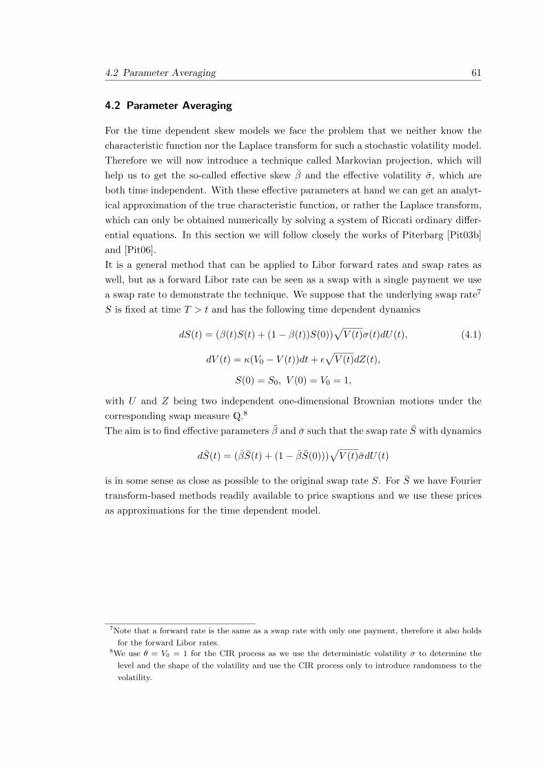
4.2 Parameter Averaging 61
4.2 Parameter Averaging
For the time dependent skew models we face the problem that we neither know the
characteristic function nor the Laplace transform for such a stochastic volatility model.
Therefore we will now introduce a technique called Markovian projection, which will
help us to get the so-called effective skew β and the effective volatility σ, which are
both time independent. With these effective parameters at hand we can get an analyt-
ical approximation of the true characteristic function, or rather the Laplace transform,
which can only be obtained numerically by solving a system of Riccati ordinary differ-
ential equations. In this section we will follow closely the works of Piterbarg [Pit03b]
and [Pit06].
It is a general method that can be applied to Libor forward rates and swap rates as
well, but as a forward Libor rate can be seen as a swap with a single payment we use
a swap rate to demonstrate the technique. We suppose that the underlying swap rate7
S is fixed at time T > t and has the following time dependent dynamics
dS(t) = (β(t)S(t) + (1− β(t))S(0))√V (t)σ(t)dU(t), (4.1)
dV (t) = κ(V0 − V (t))dt+ ε√V (t)dZ(t),
S(0) = S0, V (0) = V0 = 1,
with U and Z being two independent one-dimensional Brownian motions under the
corresponding swap measure Q.8
The aim is to find effective parameters β and σ such that the swap rate S with dynamics
dS(t) = (βS(t) + (1− βS(0)))√V (t)σdU(t)
is in some sense as close as possible to the original swap rate S. For S we have Fourier
transform-based methods readily available to price swaptions and we use these prices
as approximations for the time dependent model.
7Note that a forward rate is the same as a swap rate with only one payment, therefore it also holds
for the forward Libor rates.8We use θ = V0 = 1 for the CIR process as we use the deterministic volatility σ to determine the
level and the shape of the volatility and use the CIR process only to introduce randomness to the
volatility.

62 4 Stochastic Volatility Libor Market Model
4.2.1 Effective Skew
Theorem 4.2.1
The effective skew β for (4.1) over a time horizon [0, T ] is given by
β =
∫ T
0β(t)w(t)dt,
where the weights w(.) are given by
w(t) =y2(t)σ2(t)∫ T
0 y2(t)σ2(t)dt,
y2(t) = V 20
∫ t
0σ2(s)ds+ V0ε
2e−κt∫ t
0σ2(s)
eκs − e−κs
2κds.
This time independent function β is a weighted average of the time dependent function
β(t). More details on the effective skew can be found in Piterbarg [Pit03b].
4.2.2 Effective Volatility
After we calculated the effective skew we have the following approximate dynamics for
the underlying S
dS(t) = (βS(t) + (1− β)S(0))√V (t)σ(t)dU(t), (4.2)
dV (t) = κ(V0 − V (t))dt+ ε√V (t)dZ(t),
S(0) = S0, V (0) = V0 = 1,
with U and Z being two independent one-dimensional Brownian motions again. We
define the integrated variance process V as follows
V (T ) :=
∫ T
0σ2(t)V (t)dt.
What we want to do is to approximate European option prices for a time dependent
stochastic volatility model. So we will try to get the ATM prices as close as possible
to the original model, i.e. we want to approximate the following expectation as good
as possible
E[(S(T )− S0)+] = E[E[(S(T )− S0)+|V (.)]].
This can be seen as the expectation of a function of the integrated variance process V
E[(S(T )− S0)+] = E[E[(S(T )− S0)+|V (.)]] = E[g(V (T ))],

4.2 Parameter Averaging 63
with
g(x) =S0
β(2Φ(β
√x/2)− 1),
Φ(y) = P (η < y), η ∼ N (0, 1).
So what we have to do is to find a time independent λ solving the following equation
E
[g
(∫ T
0σ2(t)V (t)dt
)]= E
[g
(λ2
∫ T
0V (t)dt
)]. (4.3)
The calculation of these quantities is a difficult task therefore we approximate the
function g by
g(x) ≈ a+ be−cx
and get after some direct calculations, see [Pit03b], that in order to make sure that
(4.3) holds we have to solve the following equation for the effective volatility λ
ϕ
(−g′′(ξ)
g′(ξ)
)= ϕ0
(−g′′(ξ)
g′(ξ)λ2
), (4.4)
where
ξ = V0
∫ T
0σ2(t)dt.
The function ϕ is the Laplace transform of V (T ) given by
ϕ(µ) = E[exp(−µV (T ))
]. (4.5)
The function ϕ0 is defined as
ϕ0(µ) = E
[exp
(−µ∫ T
0V (t)dt
)]and corresponds to the Laplace transform of V (T ) for σ(t) ≡ 1.
The left-hand side of (4.4) has to be solved numerically9 while we can derive an explicite
solution for the right-hand side.
For (4.5) it is known10 that
ϕ(µ) = exp(A(0, T )− V0B(0, T )),
where A(t,T) and B(t,T) satisfy the Riccati system of ODEs
9For example by means of a Runge-Kutta method.10As a CIR process is from the class of the affine term structure models, see Duffie,Pan and Singleton
[DPS00].

64 4 Stochastic Volatility Libor Market Model
A′(t, T )− κV0B(t, T ) = 0,
B′(t, T )− κB(t, T )− 1
2ε2B2(t, T ) + µσ2(t) = 0,
with terminal conditions
A(T, T ) = 0,
B(T, T ) = 0.
For ϕ0(µ) we have an explicit solution
ϕ0(µ) = exp(A0(0, T )− V0B0(0, T )), (4.6)
where
B0(0, T ) =2µ(1− e−γT )
(κ+ γ)(1− e−γT ) + 2γe−γT,
A0(0, T ) =2κV0
ε2log
(2γ
(κ+ γ)(1− e−γT ) + 2γe−γT
)− 2κV0
µ
κ+ γT,
with
γ =√κ2 + 2ε2µ.
4.3 Moment Explosion in Stochastic Volatility Models
This section is taken from Andersen and Piterbarg [AP07]. While the authors consider
a broad range of stochastic volatility models we will concentrate on the following Heston
model.
Under the pricing measure we assume that for the dynamics of our underlying it holds
dX(t) = λX(t)√V (t)dWX(t), (4.7)
dV (t) = κ(θ − V (t))dt+ ε√V (t)dWV (t), (4.8)
with dWX(t)dWV (t) = ρdt, ρ ∈ (−1, 1) and λ, κ, θ, ε are positive constants. When we
want to price products with this model we have to calculate the expected value of the
underlying payoff. For some products we only need the finiteness of the first moment,
but for other products this does not suffice as they depend on higher moments.11 So
to price these products we need to make sure that the respective higher moments
E[Xw(T )], T > 0, w > 1,
stay finite. The following proposition taken from Andersen and Piterbarg [AP07] ob-
tains conditions for the finiteness of these moments.11For example for the pricing of a Libor-in-arrears, which pays the Libor rate at the fixing time, we
need to calculate a convexity adjustment, which involves the second moment.

4.3 Moment Explosion in Stochastic Volatility Models 65
Proposition 4.3.1
Consider the process (4.7). Fix
k =λ2
2w(w − 1) > 0
and define
b = 2k/ε2 > 0, a = 2(ρελw − κ)/ε2, D = a2 − 4b.
E[Xw(T )] will be finite for T < T ∗ and infinite for T ≥ T ∗, where T ∗ is given by
1. D ≥ 0, a < 0 :
T ∗ =∞.
2. D ≥ 0, a > 0 :
T ∗ = γ−1ε−2 log
(a/2 + γ
a/2− γ
), γ ≡ 1
2
√D.
3. D < 0 :
T ∗ = 2β−1ε−2(π1a<0 + arctan(2β/a)), β ≡ 1
2
√−D.
If we assume that the processes are uncorrelated we can write the moments as
E[Xw(T )] = Xw(0)EQw[exp
(k
∫ T
0V (u)du
)],
with w ≥ 0, k = λ2
2 w(w − 1) with a new measure Qw and get the following corollary.
Corollary 4.3.2
Assume that the processes X and V follow (4.7) and (4.8) with ρ = 0. Fix u > 0 and
define
b = 2u/ε2 > 0, a = −2κ/ε2, D = a2 − 4b.
Denote
Mu,w(T ) = EQw[exp
(u
∫ T
0V (s)ds
)].
• If u ≤ κ2
2ε2, then Mu,w(T ) <∞ for all T ≥ 0.
• If u > κ2
2ε2, then Mu,w(T ) =∞ for all T > T ∗ with
T ∗ = 2γ−1(π + arctan(−γ/κ)), γ =√
2ε2u− κ2.
Furthermore this also holds if we use a displaced diffusion extension and a time depen-
dent volatility function, i.e. for the process
dX(t) = λ(t)f(X(t))√V (t)dWX(t),

66 4 Stochastic Volatility Libor Market Model
dV (t) = κ(θ − V (t))dt+ ε√V (t)dWV (t),
with dWX(t)dWV (t) = ρdt, ρ ∈ (−1, 1) and κ, θ, ε are positive constants, λ a bounded
deterministic strictly positive function and f(x) = bx+h with some constants 0 < b ≤ 1
and h.
Remark 4.3.3
Collecting all the facts from above we have that the desired property
E[Xw(T )] <∞, T > 0, w > 1
holds if
λ2
2w(w − 1) ≤ κ2
2ε2.
If this is not the case we have to make sure that
T < T ∗ = 2γ−1(π + arctan(−γ/κ)), γ =√
2ε2u− κ2.
4.4 Stochastic Volatility Swap Rate Model
To get approximations for the swaption prices in the SVLMM we will make use of
a corresponding SVSMM. The dynamics of the forward rates in the SVLMM induce
dynamics for the swap rate. So we can set up a SVSMM, which yields approximately
the same dynamics for the swap rates as we get them in the SVLMM. The prices
obtained by these two models will be very close to each other, but they will not be
exactly the same.
We will look at the dynamics of a swap rate under its natural measure Qn,m and use
the same stochastic volatility process as in the Libor model. The dynamics of the swap
rate maturing at time Tn with final payment at Tm is specified as follows
dSn,m(t) = (βn,m(t)Sn,m(t) + (1− βn,m(t))Sn,m(0))√V (t)σn,m(t)dWn,m(t),
with
σn,m(t) =m−1∑i=n
qn,mi σi(t),
βn,m(t) =
m−1∑i=n
pn,mi βi(t),
qn,mi =Li(0)
Sn,m(0)
∂Sn,m(0)
∂Li(0),
pn,mi =σi(t)σn,m(t)ρi,(n,m)(t)
(m− n)|σn,m(t)|2,
ρi,(n,m)(t) =
m−1∑j=n
qn,mj ρi,j(t),

4.5 Fourier Transform-based Pricing of Products 67
where Wn,m is a one-dimensional Brownian motion under Qn,m. This yields approxi-
mately the same dynamics for the swap rate in this swap rate model as the dynamics
induced by the Libor market model. Now we can apply the parameter averaging tech-
niques that we just introduced to get the approximate dynamics
dSn,m(t) ≈ (βn,mSn,m(t) + (1− βn,m)Sn,m(0))√V (t)σn,mdW
n,m(t).
4.5 Fourier Transform-based Pricing of Products
4.5.1 Caplets
A caplet is nothing else than a European call option and therefore we can apply the
techniques for pricing these options presented in e.g. Carr and Madan [CM99], or Lord
and Kahl [LK07].
First we will deal with the displacement and then care about the stochastic volatility.
Before we can price a caplet we have to apply the parameter averaging techniques
from Section 4.2 to calculate the effective skew βi and the effective volatility σi. The
approximate price of a caplet is given as
C(0, Ti−1, Fi(0),K) ≈ P (0, Ti)Ei[(Fi(Ti−1)−K)+]
with
dFi(t) = (βiFi(t) + (1− βi)Fi(0))σi√V (t)dWi(t).
We can rewrite that as follows
C(0, Ti−1, Fi(0),K) ≈ P (0, Ti)Ei[(Fi(Ti−1)−K)+]
= P (0, Ti)Ei
[(1
βi(βiFi(Ti−1) + (1− βi)Fi(0)−K ′)
)+]
=P (0, Ti)
βiEi[(X(Ti−1)−K ′)+],
with K ′ = (βiK + (1 − βi)Fi(0)). By an easy application of Ito’s Lemma we get the
dynamics of X as follows
dX(t) = X(t)βiσi√V (t)dWi(t), X(0) = Fi(0)
and therefore we are in an undisplaced setting.12
So the task is to calculate Ei[(X(Ti−1) − K ′)+], which is a general European option
pricing problem, which can be solved by the help of Fourier methods. As this is not
12For details see Andersen and Andreasen [AA02]. Note that the formula does not work for βi = 0,
but can be adjusted for the case βi < 0.

68 4 Stochastic Volatility Libor Market Model
specific for caplets we will do this in a rather general fashion and therefore we denote
the underlying by ST and for convenience reasons we denote the price of the European
option in the following by CT (K) := C(0, T, S0,K).
We have a one-to-one correspondence between the characteristic function and the den-
sity of a random variable, because the characteristic function uniquely determines the
distribution.
The following is mainly taken from Carr and Madan [CM99]. The characteristic func-
tion of a random variable sT = lnST is given as
ΦT (u) = E[exp(iusT )] =
∫ ∞−∞
eiusqT (s)ds,
where we denote by qT (s) the density of the random variable.
We want to calculate the price of a European call option on this random variable, i.e.
CT (k) = E[e−rT (esT − ek)+] =
∫ ∞k
e−rT (es − ek)qT (s)ds,
with k = lnK.
To avoid some integrability problems described in Carr and Madan [CM99] we instead
use the exponentially dampened price
cT (k) = eαkCT (k), α > 0.
The Fourier transform of cT (k) is then given as
ψT (u) =
∫ ∞−∞
eiuscT (s)ds.
In some models especially in the Heston model we have an explicit formula for this
Fourier transform available. If we use the inverse formula we get the dampened price,
i.e.
CT (k) =e−αk
2π
∫ ∞−∞
e−ikvψT (v)dv.
If we furthermore make use of the symmetry of the Fourier transform we can write this
as
CT (k) =e−αk
π
∫ ∞0
e−ikvψT (v)dv.
We know that the Fourier transform of a European call option is given as
ψT (v) =e−rTΦT (v − (α+ 1)i)
α2 + α− v2 + i(2α+ 1)v.
So we are now in the position to calculate option prices if we have a formula for the
characteristic function ΦT (u) of the random variable.
4.5 Fourier Transform-based Pricing of Products 69
Remark 4.5.1 (Heston characteristic function and the Heston trap)
When we calculate the option prices with the help of the Fourier transformation we
have to evaluate a complex logarithm, which might lead to discontinuities.
If we use the following version of the characteristic function
ΦT (u) := exp(iu(logS0 + rT ))
× exp(θκε−2((κ− ρεiu− d)T − 2 log((1− ge−dT )/(1− g))))
× exp(V 20 ε−2(κ− ρεiu− d)(1− e−dT )/(1− ge−dT )),
with
d =√
(ρεui− κ)2 + ε2(iu+ u2),
and
g = (κ− ρεiu− d)/(κ− ρεiu+ d),
we get the correct values and do not need to use a rotation count algorithm presented
in Lord and Kahl [LK06].13 For more details on the Heston Trap see Fahrner [Fah07]
and Lord and Kahl [LK06].
4.5.2 Swaptions
We look at a swap rate with first fixing date Tn and last payment date Tm and remember
that the formula for a swap rate is given by
Sn,m(t) =P (t, Tn)− P (t, Tm)∑m
i=n+1 τiP (t, Ti).
If we choose∑m
i=n+1 τiP (t, Ti) as numeraire we work under the swap measure and know
that the swap rate in this case is a martingale.
By specifying the stochastic volatility Libor market model (SVLMM) we also specify
the dynamics of the swap rates. We now try to find a stochastic volatility swap market
model (SVSMM) that is as close as possible to these implied dynamics coming from
the SVLMM. We achieve that by using the following dynamics under the swap measure
Qn,m
dSn,m(t) = (βn,m(t)Sn,m(t) + (1− βn,m(t))Sn,m(0))√V (t)σn,m(t)dWn,m(t), (4.9)
where Wn,m(t) is a one-dimensional Brownian motion under Qn,m and the functions
βn,m(t) and σn,m(t) are calculated as stated in Section 4.4. The stochastic volatility
process V stays the same after the measure change, so we use the same process as in
the SVLMM. We are now in the same setting as we were for caplets in the SVLMM
13In our case the correlation between the Libor rate and the stochastic volatility is ρ = 0 and θ = 1.

70 4 Stochastic Volatility Libor Market Model
and therefore we make again use of the parameter averaging technique described in
Section 4.2 to calculate the effective parameters βn,m and σn,m and get the following
approximate dynamics
dSn,m(t) = (βn,mSn,m(t) + (1− βn,m)Sn,m(0))√V (t)σn,mdW
n,m(t).
For this time independent SVSMM we have an approximate swaption pricing formula
based on Fourier transformation as shown above.
4.5.3 CMS Spread Options
As already mentioned to get a realistic correlation structure we have to calibrate the
model to the historically estimated correlation matrix, or to correlation sensitive prod-
ucts. Although we have liquidly traded correlation sensitive products readily available,
namely swaptions, their dependence on the correlation is very weak. They only depend
on the overall level of correlation and not on the specific shape. Furthermore we have
already shown that a descent decorrelation can also be produced by the choice of the
volatility function. If one wants to calibrate the correlation to historical data one faces
two problems. The first problem is the estimation of the historical correlation. We
must decide how to strip the yield curve, which data we use and which estimation and
smoothing methods we want to use. The second problem is that after we estimated
the correlation matrix we mix up a forward looking calibration of the volatilities and
a backwards looking view on the correlation which is, although Girsanov’s theorem
tells us that the correlations will stay the same after a change of measure, somehow
inconsistent. We would rather prefer to calibrate both the volatility and the correla-
tion structure to forward looking products. A CMS spread option is a liquidly traded
product that depends heavily on the level and shape of the correlation matrix. In the
following we will have a look at two possibilities to approximate the prices of these
products in order to include them in a calibration. As the second approach is more
intuitive, easier to implement and faster than the first approach we will only briefly
introduce the idea of the approach taken by Antonov and Arneguy [AA09].
Antonov and Arneguy Approach
As we already stated before the price of a CMS spread option paying at time T is given
as follows
CMSSO(0) = P (0, T )ET [(S1(T )− S2(T )−K)+], (4.10)
where S1 and S2 are two swap rates and K is the strike of the option. The problem of
evaluating (4.10) is that S1 and S2 are not martingales under the T forward measure.
What we will do is to change the measure to the spread measure under which the

4.5 Fourier Transform-based Pricing of Products 71
difference S1(t)− S2(t) is a martingale, i.e.
CMSSO(0) = P (0, T )ET [(S1(T )−S2(T )−K)+] = P (0, T )E[(S1(T )−S2(T )−K)+M(T )],
where M is the Radon-Nikodym derivative introduced by the measure change, which
is actually hard to compute. Furthermore we still have the problem that we do not
know the joint dynamics of M(t) and S(t) = (S1(t)− S2(t)). The crucial point in this
situation is to approximate the process M linearly for CMS pricing or non-linearly in
case of CMS spread option pricing.
We now look at a general function f(S(t)), with S(t) denoting for example a swap rate,
or as above the difference of two swap rates and V denoting the price
V = P (0, T )ET [f(S(t))] = P (0, T )ES [f(S(t))M(t)].
In the following we will skip the S in the notation, but we still work under the S
martingale measure, i.e. E[f(S(t))M(t)] = ES [f(S(t))M(t)].
We know by the tower law of expectations that
E[f(S(t))M(t)] = E[f(S(t))E[M(t)|S(t)]]
and now we want to approximate
E[M(t)|S(t)].
Linear approximation:
E[M(t)|S(t)] ≈ A(t) +B(t)S(t).
A solution to this easy problem of minimizing
E[(M(t)−A(t)−B(t)S(t))2]
can be obtained as follows
B(t) =E[M(t)S(t)]− S0
V ar[S(t)]=ET [S(t)]− S0
V ar[S(t)],
A(t) = 1−B(t)S0,
so in this linear case we have
E[f(S(t))M(t)] = E[f(S(t))E[M(t)|S(t)]]
≈ E[f(S(t))(A(t) +B(t)S(t))]
= E[f(S(t))] +B(t)E[f(S(t))(S(t)− S(0))].

72 4 Stochastic Volatility Libor Market Model
The authors derive approximate formulas for these expectations and finally calculate
the price by means of a one-dimensional Fourier inversion. While this approximation
works well for products like a CMS we have to use a non-linear approximation for more
complicated products like CMS spread options.
Non-linear approximation:
The authors show that a linear approximation is not sufficient for CMS spread options
therefore they use a non-linear approximation. With S(t) := S1(t)−S2(t) and ∆S(t) :=
S(t)− S(0) the approximation we use looks as follows
E[M(t)|S(t)] ≈ A(t) +B(t)∆S(t) + C(t)[∆S(t)+].
In this case we have to minimize the following function
E[(M(t)−A(t)−B(t)∆S(t) + C(t)[∆S(t)+])2]
and with E[M(t)] = 1, the solution can be calculated as the solution of the following
system of equations
1 = A+ CE[∆S(t)+]
ET [∆S(t)] = BE[∆S(t)2] + CE[(∆S(t)+)2]
ET [∆S(t)+] = AE[∆S(t)+] +BE[(∆S(t)+)2] + CE[(∆S(t)+)2].
The authors again derive some approximations and finally calculate the prices by means
of a nontrivial and computationally expensive two dimensional Fourier inversion.
E[(S(T )−K)+M(t)] = E[(S1(T )− S2(T )−K)+E[M(t)|S(t)]]
≈ E[(S1(T )− S2(T )−K)+(A(t) +B(t)∆S(t) + C(t)[∆S(t)+])]
Furthermore many numerical problems might occur when we calculate these integrals.
Remark 4.5.2
We collect the findings. At a first glance the Antonov and Arneguy approach looks quite
appealing and easy to implement, but actually it is rather complicated to implement and
to calculate prices we have to calculate a Fourier inversion in two dimensions which
is a non-trivial task and computationally demanding. Therefore we prefer the method
introduced in the following.

4.5 Fourier Transform-based Pricing of Products 73
Lutz and Kiesel Approach
The approach introduced by Lutz and Kiesel [LK10b] is based on conditional expecta-
tions. In Section 2.4.3 we have introduced an approximation for spread option prices in
a Libor market model, i.e. we can calculate the price if the volatility is deterministic.
So if we work under the Tn+1 forward measure14 Qn+1 and forget a second about the
skew by setting it to one we can calculate the price of a spread option paying at time
Tn+1 as follows
P (0, Tn+1)E[(S1(Tn)− S2(Tn)−K)+] = P (0, Tn+1)E[E[(S1(Tn)− S2(Tn)−K)+|V = v]]
= P (0, Tn+1)E[CLMM (0, Tn,K; V )]
= P (0, Tn+1)
∫ ∞0
CLMM (0, Tn,K; v)f(v)dv,
where CLMM (0, Tn,K; v) denotes the spread option price in a Libor market model if the
integrated stochastic variance process V =∫ Tn
0 V (t)dt is equal to v and f(v) denotes
the density of V . We do not know the density f explicitly, we only know the Fourier
transform of it and therefore we can calculate it only by Fourier inversion, but this
inversion is very time consuming. There are some possibilities to speed up the calcu-
lation of the Fourier inversion which makes it possible to use it for calibration purposes.
With x ≥ 0 the density f can be calculated as follows
f(x) =1
2πi
∫ a+i∞
a−i∞exsf(s)ds
=1
2π
∫ ∞∞
ex(a+is)f(a+ is)ds
=1
π
∫ ∞∞
Re(ex(a+is)f(a+ is)
)ds,
where Re() denotes the real part and f is the Laplace transform of V . In the last step
we made use of the fact that this is a symmetric function.
In this standard formula we integrate along the line
s(u) = a+ iu.
The integrand is oscillating very much on this line making it hard to integrate the
function. If we use a different line along which we integrate, to be precise we will use
s(u) = a+ u(bi− a), (4.11)
we can get a much nicer function with less oszillations. It remains to determine how
to choose a, b > 0 in order to get an optimal linear contour, which is done in Lutz
14For convenience reasons we write E instead of En+1.

74 4 Stochastic Volatility Libor Market Model
and Kiesel [LK10b] by means of Newton’s method. When we use (4.11) we get for the
density
f(x) =1
π
∫ ∞0
Im(ex(a+u(bi−a))f(a+ u(bi− a))(bi− a)
)du, x ≥ 0.
If we calculate the value of the integral from 0 to ∞ numerically we have to cut the
integral at some point and therefore make a truncation error. But there is an easy
transformation function such that we only have to integrate from 0 to 1 and get rid of
the truncation error.
With
s(u) = a− 3log(u)(bi− a)
and
s′(u) = −3
u(bi− a),
we get
f(x) = − 1
π
∫ 1
0Im(exs(u))f(s(u)))s′(u)
)du, x ≥ 0.
For each underlying swap rate we assume the following dynamics
dSi(t) = (βiSi(t) + (1− βi)Si(0))√V (t)σidW
Si(t), i = 1, 2,
with the effective volatilities σi and the effective skews βi calculated as described in
Section 4.2 and correlated one-dimensional Brownian motions WSi under QSi ,15 with
dWS1(t)dWS2(t) = ρ1,2(t)dt.
If we work under the Tn+1 forward measure we introduce a drift µi(t) for i = 1, 2 to
the dynamics of the swap rates, which can be calculated similarly as in Section 2.4.3.
Under Qn+1 we approximate the dynamics by
dSi(t) = µiV (t)dt+ (βiSi(t) + (1− βi)Si(0))√V (t)σidW
Si(t), i = 1, 2,
We make use of the same techniques as in Section 4.5.1 to deal with the skew and define
σi = βiσi
µi :=µiβiSi(0)
, i = 1, 2,
where we made use of the freezing the drift technique for µi. The price is then calculated
as follows
P (0, Tn+1)E[(S1(Tn)− S2(Tn)−K)+]
≈ P (0, Tn+1)
∫ ∞0
∫ ∞−∞
g(u, v)1√2πe−
12u2duf(v)dv,
15QSi denotes the respective swap measure.

4.6 A New Approximative Terminal Correlation Formula 75
with
g(u, v) =
S1(0)
β1exp(h(u, v))− K(u, v) , K(u, v) ≤ 0,
S1(0)
β1exp(h(u, v))Φ
log
(S1(0)
β1K(u,v)
)+h(u,v)+ 1
2σ2
1(1−ρ2)v
σ1
√v(1−ρ2)
, K(u, v) > 0,
−K(u, v)Φ
log
(S1(0)
β1K(u,v)
)+h(u,v)− 1
2σ2
1(1−ρ2)v
σ1
√v(1−ρ2)
K(u, v) =
S2(0)
β2exp
[(µ2 −
1
2σ2
)v + σ2
√vu
]+ K,
K =1− β1
β1S1(0)− 1− β2
β2S2(0) +K,
h(u, v) =
(µ1 −
1
2ρ2σ1
)v + ρσ1
√vu.
We approximate the correlation as follows
ρ =
∫ Tn0 σ1(t)σ2(t)ρ1,2(t)dt√∫ Tn
0 σ1(t)2dt√∫ Tn
0 σ2(t)2dt.
4.6 A New Approximative Terminal Correlation Formula
We intend to find a more accurate approximative formula for the terminal correlation
between two arbitrary forward rates.16 To accomplish this task we will make use of the
Markovian projection technique described in Section 4.2. Working under the terminal
measure QM we know that
dFk(t)
(Fk(t) + αk)= σk(t)
√V (t)[−
√V (t)
M∑j=k+1
τjρkjσj(t)(Fj(t) + αj)
1 + τjFj(t)︸ ︷︷ ︸=:µk(t)
dt+ dWk(t)]
dV (t) = κ(θ − V (t))dt+ ε√V (t)dZ(t),
with dWk(t)dZ(t) = 0dt and dWk(t)dWj(t) = ρk,jdt for j, k ∈ 1, ...,M.
16This might be used for the calibration to the empirically observed correlation matrix, or for pricing
correlation sensitive products.

76 4 Stochastic Volatility Libor Market Model
Proposition 4.6.1
Let w.l.o.g. 0 ≤ T ≤ Ti−1 ≤ Tj−1, then the terminal correlation between two forward
rates Fi and Fj with i ∈ 1, ...,M, j ∈ i, ...,M at time T under the terminal
measure17 QM can be approximated by
CorrM (Fi(T ), Fj(T ), 0, T ) ≈ ρi,jσ2i,j
σiσj,
where σi is the effective volatility parameter and σ2i,j we call the effective covariance
parameter,18 which we get by applying the Markovian projection method from Section
4.2 to∫ T
0 ρi,jσi(t)σj(t)V (t)dt.
Proof. We have seen in Section 3.1.2 that in case we have a skew parameter αk > 0 we
can calculate it in the same way as for the case αk = 0 for all k = 1, ...,M . Therefore
we set αk = 0 for all k = 1, ...,M . If we assume for a moment that we know the path
of the stochastic volatility process V then we have for all k = 1, ...,M
dFk(t) = Fk(t)µk(t)dt+ Fk(t)σk(t)√V (t)dWk(t),
with
µk(t) = σk(t)√V (t)µk(t).
For this SDE we can provide the following solution
Fk(Tα) = Fk(0) exp
(∫ Tα
0µk(t)−
σ2k(t)V (t)
2dt+
∫ Tα
0σk(t)
√V (t)dWk(t)
).
The product of two forward Libor rates then looks as follows
Fi(T )Fj(T ) =Fi(0)Fj(0) exp
(∫ T
0µi(t) + µj(t)−
σ2i (t) + σ2
j (t)
2V (t)dt
)
exp
(∫ T
0σi(t)
√V (t)dWi(t) +
∫ T
0σj(t)
√V (t)dWj(t)
).
If we fix the path of the stochastic volatility process V , then the two dimensional
random vector (∫ T
0σi(t)
√V (t)dWi(t),
∫ T
0σj(t)
√V (t)dWj(t)
)is jointly normally distributed with mean (0, 0) and covariance matrix
∫ T0 σ2
i (t)V (t)dt ρi,j∫ T
0 σi(t)σj(t)V (t)dt
ρi,j∫ T
0 σi(t)σj(t)V (t)dt∫ T
0 σ2j (t)V (t)dt
.
17We could have choosen any measure Qγ as long as T ≤ Tγ .18For details see the proof of the proposition.

4.6 A New Approximative Terminal Correlation Formula 77
If we define Yk :=∫ T
0 µk(t)dt and apply the freezing the drift approximation then we
know that the only source of randomness in Yk comes from the stochastic volatility.
Therefore if we fix the path of the stochastic volatility Yk becomes deterministic. We
now calculate the conditional expectation conditioned on the path of the stochastic
volatility process. Note that we work under the measure QM and skip the M again for
notational convenience, i.e. we write E instead of EM .
E[Fi(T )|V ] = E
[Fi(0) exp
(∫ T
0µi(t)−
σ2i (t)V (t)
2dt+
∫ T
0σi(t)
√V (t)dWi(t)
)|V]
= Fi(0) exp
(∫ T
0µi(t)
)= Fi(0) exp(Yi),
E[Fi(T )2|V ] = Fi(0)2E
[exp
(2Yi −
∫ T
0σ2i (t)V (t)dt+
∫ T
02σi(t)
√V (t)dWi(t)
)|V]
= Fi(0)2 exp
(2Yi +
∫ T
0ρi,iσi(t)σi(t)V (t)dt
)= Fi(0)2 exp
(2Yi +
∫ T
0σ2i (t)V (t)dt
)
and
E[Fi(T )Fj(T )|V ] = E
[Fi(0)Fj(0) exp
(∫ T
0µi(t) + µj(t)−
σ2k(t) + σ2
j (t)
2V (t)dt
)
exp
(∫ T
0σi(t)
√V (t)dWi(t) +
∫ T
0σj(t)
√V (t)dWj(t)
)|V]
= Fi(0)Fj(0) exp
(∫ T
0µi(t) + µj(t)dt+
∫ T
0ρi,jσi(t)σj(t)V (t)dt
)= Fi(0)Fj(0) exp
(Yi + Yj +
∫ T
0ρi,jσi(t)σj(t)V (t)dt
).
The correlation can the be calculated as follows

78 4 Stochastic Volatility Libor Market Model
CorrM (Fi(T ), Fj(T ), 0, T ) =
=E[Fi(T )Fj(T )]− E[Fi(T )]E[Fj(T )]√
E[F 2i (T )]− E[Fi(T )]2
√E[F 2
j (T )]− E[Fj(T )]2
=E[E[Fi(T )Fj(T )|V ]]− E[E[Fi(T )|V ]]E[E[Fj(T )|V ]]√
E[E[F 2i (T )|V ]]− E[E[Fi(T )|V ]]2
√E[E[F 2
j (T )|V ]]− E[E[Fj(T )|V ]]2
=Fi(0)Fj(0)
(E[exp(Yi + Yj +
∫ T0 ρi,jσi(t)σj(t)V (t)dt)]− E[exp(Yi)]E[exp(Yj)]
)√E[E[F 2
i (T )|V ]]− E[E[Fi(T )|V ]]2√E[E[F 2
j (T )|V ]]− E[E[Fj(T )|V ]]2
=
(E[exp(Yi + Yj +
∫ T0 ρi,jσi(t)σj(t)V (t)dt)]− E[exp(Yi)]E[exp(Yj)]
)√E[exp(2Yi + Σi)]− E[exp(Yi)]2
√E[exp(2Yj + Σj)]− E[exp(Yj)]2
,
with Σk =∫ T
0 σk(t)V (t)dt,∀k = 1, ...,M .
Now we freeze the stochastic volatility in the drift, i.e.
µk(t) = σk(t)√V (t)µk(t) ≈ σk(t)
√V (0)µ0
k(t),
with
µ0k(t) := −
√V (0)
M∑j=k+1
τjρkjσj(t)(Fj(0) + αj)
1 + τjFj(0),
or at some average level in between V (0) and θ. Furthermore we define
Y 0k :=
∫ T
0µ0k(t)dt, ∀k = 1, ...,M.
The error we make is not too big for the terminal correlation as we do it for all rates
and divide the drifts by each other.19 Then the drift is deterministic and we can take
it out of the expectation
CorrM (Fi(T ), Fj(T ), 0, T ) ≈
≈exp(Y 0
i + Y 0j )E[exp
∫ T0 ρi,jσi(t)σj(t)V (t)dt]− exp(Y 0
i ) exp(Y 0j )
exp(Y 0i + Y 0
j )√E[exp(
∫ T0 σ2
i (t)V (t)dt)]− 1√E[exp(
∫ T0 σ2
j (t)V (t)dt)]− 1
≈E[exp(
∫ T0 ρi,jσi(t)σj(t)V (t))dt]− 1√
E[exp(∫ T
0 σ2i (t)V (t)dt)]− 1
√E[exp(
∫ T0 σ2
j (t)V (t)dt)]− 1.
With the parameter averaging technique in the first step followed by a first order
approximation in the second step we can write this as
19But a thorough analysis has to be performed if we actually want to use it. As we will not use the
approximation for our calibration we will not perform this analysis.

4.6 A New Approximative Terminal Correlation Formula 79
CorrM (Fi(T ), Fj(T ), 0, T ) ≈E[exp(σi,j
∫ T0 V (t)dt)]− 1√
E[exp(σ2i
∫ T0 V (t)dt)]− 1
√E[exp(σ2
j
∫ T0 V (t)dt)]− 1
≈E[σi,j
∫ T0 V (t)dt]√
E[σ2i
∫ T0 V (t)dt]
√E[σ2
j
∫ T0 V (t)dt]
=σi,jE[
∫ T0 V (t)dt]
σiσj
√E[∫ T
0 V (t)dt]√E[∫ T
0 V (t)dt]
=σi,jσiσj
.
Corollary 4.6.2
Let w.l.o.g. 0 ≤ T ≤ Ti−1 ≤ Tj−1, then the terminal correlation between two forward
rates Fi and Fj with i ∈ 1, ...,M, j ∈ i, ...,M at time T under the terminal
measure20 QM can be approximated by
CorrM (Fi(T ), Fj(T ), 0, T ) =E[exp(
∫ T0 ρi,jσi(t)σj(t)V (t)dt)]− 1√
E[exp(∫ T
0 σ2i (t)V (t)dt)]− 1
√E[exp(
∫ T0 σ2
j (t)V (t)dt)]− 1.
Proof. The corollary follows directly from the proof of the proposition.
Remark 4.6.3
The expectations from above are equal to the Laplace transform of the respective inte-
grated processes and therefore we only have to solve a system of Riccati ODEs in order
to obtain the expectations.21 Therefore all of the expectations in the corollary above can
be calculated numerically by means of e.g. Runge-Kutta methods.
Remark 4.6.4
In our model we have set θ = V0 = 1 so the stochastic volatility process will be around
the level 1. In this case the approximation (2.11) will do a good job and we do not have
to perform these calculations. But if the mean level is far away from the initial level
this might introduce decorrelation and this should be taken into account.
20We could have choosen any measure Qγ as long as T ≤ Tγ .21The procedure is exactly the same as in the parameter averaging technique introduced in Section
4.2.

80 4 Stochastic Volatility Libor Market Model
4.7 Calibration to Swaptions
We will only deal with swaption calibration as a caplet can be interpreted as a swaption
depending only on one forward rate. For the calibration to swaptions we have many
choices how to proceed. We will now first introduce the basic idea and then show how
we can speed up the calibration and make it more robust by splitting it in a two or
three step calibration. In the following section we will deal with the case where we have
a set of good starting parameters already available and perform a local search, before
we think about global calibration in Section 4.7.2 without initial guess.
4.7.1 Daily Calibration Algorithm
The first idea to calibrate the model is to calibrate all parameters directly to the
observed caplet and swaption prices. We can calculate these prices by help of the
approximations introduced in Section 4.5.2 and compare them to the observed prices
in the market. So the optimization would look as follows
min(a,b,c,d,Φ,ρ,β,v)
K∑i=1
wi g(CMkti − Cmodeli (a, b, c, d, Φ, ρ, β, v)),
where g is a suitable function as defined in Section 2.5, vector w = (w1, ..., wK) denotes
a vector of weights, Φ = (Φ1, ...,ΦM ) denotes the time inhomogeneity factors, v = [κ, ε]
denotes the vector of parameters determining the dynamics of the stochastic volatility
process. We set θ = 1 and later we will choose some realistic value for κ, e.g κ = 0.2
before we start the calibration. ρ denotes the vector of correlation parameters and β the
skew parameters, both depending on the chosen parametrization with some constraints
on the parameters.22 CMkti for i = 1, ...,K denote the market prices of the products.
We denote the number of overall parameters by N and we must make sure that for the
number of products K we calibrate the model to, it holds K ≥ N to obtain meaningful
parameters. The function Cmodeli : RN 7→ R yields the model price calculated for the
parameter set.
If we went that way to calibrate the model, the calibration algorithm would be much
too slow to use it in everyday practice, but the special structure of the approximation
for the prices allows for much more comfortable and faster calibration approaches.
Instead of fitting the observed prices directly we will first do a pre-calibration step
where we fit a single SVSMM to each swaption smile with a joint volatility of volatility
parameter. Then we will use this matrix of pre-calibrated parameters as input for the
main-calibration. This two step calibration can be found in Piterbarg [Pit03b] and will
be introduced in the following.
22The volatility, correlation and skew parameters have to be within some bounds, for details see Sections
2.3.3 and 2.3.4.

4.7 Calibration to Swaptions 81
Pre-Calibration
In this step we fit one single time independent SVSMM to the swaption smile of each
swap rate separately and get a matrix of calibrated parameters. To calibrate one
swaption smile we have four parameters at hand β, σ, κ and ε, but if we have a closer
look at the relationship between the speed of mean reversion κ and the volatility of
volatility parameter ε we can see that in case we increase both we get similar dynamics
for the model, i.e. we get similar prices for the products we wish to calibrate the model
to. Therefore we will fix the speed of mean reversion at a level between 10% and 20%
as suggested by Piterbarg in [Pit03b] .
The calibration for each single swap rate looks as follows
min(βn,σn,εn)
Kn∑i=1
wi g(CMkti,n − Cprei,n (β, σ, ε)),
if we want to calibrate a swaption smile observed from K market quotes. The function
Cprei,n : R3 7→ R denotes the price of a swaption in the time independent swap market
model, see Section 4.5.2. The i index denotes different strikes and the n index different
maturities for the swaptions. Actually we would have to account for the different tenors
as well, but for the ease of notation we skip the tenor m and just assume we calibrate
it to swaptions with different maturities but the same tenor.
So we get three parameters for each swap rate Sn,m, namely βn,m, σn,m and εn,m. For
the stochastic volatility we have to keep in mind that we have one stochastic volatility
process for all forward Libor rates. Therefore we should calibrate one joint volatility
of volatility (volofvol) parameter ε for all smiles. So we have two possibilities, either
we set ε to some average of the calibrated εn,ms and restart the single calibrations with
only two parameters and use the previously calibrated parameters as starting values,
i.e.
min(βn,σn)
Kn∑i=1
wi g(CMkti − Cmodeli (βn, σn, ε))
for each swap rate Sn,m.
Or we calibrate it jointly by solving the larger minimization problem
min(β1,...,βk,...,σ1,...,σk,ε)
k∑n=1
Kn∑i=1
wi g(CMkti,n − Cprei,n (βn, σn, ε)).
if we want to calibrate k swaption or caplet smiles and we have Kn market quotes for
each swaption smile respectively.23
23To actually calibrate the smile we should at least have Kn ≥ 3 for all n = 1, ..., k.

82 4 Stochastic Volatility Libor Market Model
As this pre-calibration is quite easy to do by a local search algorithm like Levenberg-
Marquardt and because it is quite fast and stable we will use the second more precise
approach. Furthermore we have to make sure in the minimization that the following
constraints are fulfilled
σ > 0,
ε ≥ 0.
If we set ε = 0 we do not have any stochastic volatility anymore and the volatility
is deterministic again, i.e. we are back in a displaced diffusion Libor market model
setting, but due to numerical instabilities and division through zero we have to be
careful and make sure that the volatility of volatility does not become too small, i.e.
ε ≥ h,
with h small.24
Remark 4.7.1
When we actually want to perform the calibration we face the problem that we have to
choose some starting values. If we have performed a calibration the day before we can
take these values as starting values. If not we have to do a global optimization. But
this problem is so well-behaved that we can just choose some realistic average level for
the parameters and do a local search. This pre-calibration step is very stable and we
would have to make up very unrealistic parameter values to get in trouble at this stage.
So after the pre-calibration we have 2k+1 estimated parameters βpre = (βpre1 , ..., βprek ),
σpre = (σpre1 , ..., σprek ) and εpre.
Main-Calibration
As already stated above we now use the pre-calibrated skew and volatility matrices
as market input and try to find the parameters which yield model implied effective
volatilities and skews as close as possible to them.
To actually do so we have different possibilities. In any case we set the volatility of
volatility parameter ε equal to the estimated joint parameter εpre and then we have two
options:
24For our calculations we used h = 10−4 which is very close to the deterministic case, but avoids
numerical instabilities. For smaller values we encountered some severe problems.

4.7 Calibration to Swaptions 83
1. Calibrate all at once
min(a,b,c,d,Φ,ρ,β)
k∑i=1
(wi g1(σprei − σmodeli (a, b, c, d, Φ, ρ, β))
+ wk+i g2(βprei − βmodeli (a, b, c, d, Φ, ρ, β))
)for the k market smiles with the weight vector w = (w1, ..., w2k) and some distance
functions g1 and g2 defined as in Section 2.5. Note that this does not depend on
the stochastic volatility parameters v = (κ, ε) as we set κ to a realistic value and
calibrated ε already in the pre-calibration.
2. We split the calibration problem up in two or rather three steps. As already
mentioned the big advantage of the parametrization used by Piterbarg is that the
volatility parameters are at least almost independent of the skew parameters and
therefore we can calibrate them separately.
Step 1: Volatility and Correlation
In a first step we set all effective skew values to the pre-calibrated values25 and
solve
min(a,b,c,d,Φ,ρ)
k∑i=1
wi g1(σprei − σmodeli (a, b, c, d, Φ, ρ)),
so we calibrate the volatility and correlation parameters to the pre-calibrated
effective volatilities σpre.
Again as before if we wish to get the Φ’s as close as possible to one, i.e. to make
the model as time homogeneous as possible we can add a penalty factor as in
Section 2.5.26
Step 2: Skew
In this step we calibrate the skew parameters in our abcd parametrization βa, βb, βc
and βd to the pre-calibrated effective skew
minβ
k∑i=1
wk+i g2(βprei − βmodeli (a, b, c, d, Φ, ρ, β)).
25In Piterbarg [Pit03b] the author sets the βs to some average skew level, but the pre-calibrated values
are a much better guess of final values of the skews therefore we use these estimates instead of the
artificially introduced guess.26If we introduce a penalty factor in Step 1 we obviously have to do the same in Step 3.

84 4 Stochastic Volatility Libor Market Model
Step 3: Volatility and Correlation
Repeat the first step with the calibrated displacement parameters
min(a,b,c,d,Φ,ρ)
k∑i=1
wi g1(σprei − σmodeli (a, b, c, d, Φ, ρ)).
Remark 4.7.2
When we actually do the calibration we see that we get a very descent fit already after
the second step, therefore we can omit the third step.
4.7.2 Initial Calibration Algorithm
The calibration routine described in the previous section works perfectly fine if we
have good starting values readily available, for example from a calibration done the
day before. But from time to time one may wish to check whether the calibrated
parameters are really still the global optimum, or if there is a set of parameters which
fits the market better. Furthermore after having implemented the model we have to do
a first initial calibration and have no starting values at hand. In this case we might have
some trouble because if we choose an arbitrary set of parameters and do an optimization
with a fast local optimization algorithm we will most likely end up in a local minimum
and not in the global minimum. So we have to resort to global optimizers, but this
is usually very time consuming especially in our case as the error function in the first
step is computationally quite expensive due to the numerical solution of the system of
Riccati ODEs necessary for the effective volatility calculation. Therefore we have to
speed up the calibration routine. What we will do is to use an approximation of the
effective volatility for the global optimization. Once we have this global minimum at
hand we start a local search from this parameter set using the correct effective volatility.
We remind the reader that we stated in Section 4.2 that in order to calculate the
effective volatility σ we have to make sure that the following equation holds
ϕ (−η) = ϕ0(−ησ2). (4.12)
There are many possibilities how to approximate the effective volatility. In the following
we will discuss three of them.
• Piecewise constant approximation of the abcd volatility curve.
• Rebonato’s formula.
• Displaced version of Rebonato’s formula.

4.7 Calibration to Swaptions 85
Piecewise constant:
We now want to approximate the left side of (4.12) by an easier term, which we can
calculate explicitly and we do not have to solve a system of Riccati ODEs.
Instead of the original volatility function σ(t) we use a piecewise constant approximation
of this function. In case of a piecewise constant function the function ϕ can be calculated
explicitly, see for example Mathew [Mat09].
Rebonato’s formula:
Another possibility is to say we let the volatility be deterministic for a moment, i.e.
ε = 0. If we also set the displacement to 1 we have
ϕ (−η) = E[e−η∫ T0 σ2(t)1dt] = e−η
∫ T0 σ2(t)dt,
ϕ0(−ησ2) = E[e−ησ2∫ T0 1dt] = e−ησ
2T ,
so we can calculate the effective volatility directly by
σ2 =1
T
∫ T
0σ2(t)dt =
1
T(vLMM (T ))2
and do not need to make use of a root finding algorithm. The idea is that the effective
volatility is some kind of average level of volatility. The Rebonato formula is exactly
the same, an average level of volatility for the deterministic case. But using this as an
approximation is not too bad as the stochastic volatility’s starting value V0 and level of
mean reversion is θ are both equal to one. If we had assumed different starting values
and levels of mean reversion we might have to think about whether this approximation
is still good enough or not.
Displaced Rebonato’s formula:
If we use the correct displacement instead of setting it to one we can not use Rebon-
ato’s formula, but there is a displaced version available. We will get a slightly better
approximation in this case, but the effective volatility depends only weakly on the
displacement.
So again we have
σ2 =1
T
∫ T
0σ2(t)dt =
1
T(vDDLMM (T ))2,
with the displaced version of Rebonato’s formula for the integral. This would be very
appealing in case we wanted to calibrate a SVLMM with displacement function φ(x, t) =
x+ b.
The approximation which yields the closest values is the first piecewise constant ap-
proach, but this is also the approach which is the computationally most expensive one

86 4 Stochastic Volatility Libor Market Model
Rebonato Piecewise constant
pro very fast precision
no extra effort to implement it
con precision extra implementation effort
slower
Table 4.1: Qualitative comparison of the approximations.
as we still have to use a root finding algorithm to find the effective volatility σ. Fur-
thermore we have to implement the piecewise constant approximation and calculate
the product of the Laplace transforms.
Rebonato’s formulas are much faster as we calculate the effective volatility directly
and do not need to search for any roots. Furthermore if we have implemented a Libor
market model or a displaced Libor market model beforehand anyway,27 then we have
the Rebonato approximation already available and do not have to implement and test
them before we can use them and we do not have to specify a time grid. We will
use the Rebonato approximation and denote the effective volatility coming from this
approximation by σapprox. The calibration routine then looks as follows:
1. Use a global optimizer to calibrate the model, by making use of one of the ap-
proximate formulas for the effective volatility, to the pre-calibrated volatilities28
min(a,b,c,d,Φ,ρ)
k∑i=1
wi g1(σprei − σapproxi (a, b, c, d, Φ, ρ)).
2. Set all skew parameters βn,m to the pre-calibrated values29 β = βpre then solve
by means of a local optimizer
min(a,b,c,d,Φ,ρ)
k∑i=1
wi g2(σprei − σSV LMMi (a, b, c, d, Φ, ρ)).
3. Calibrate the skew
minβ
k∑i=1
wi g3(βprei − βSV LMMi (a, b, c, d, Φ, ρ, β)).
27Which is most likely as no one will start with a stochastic volatility model if he has no experience
with a deterministic model.28It is important to calibrate it to the effective volatilities and not to the ATM swaption volatilities as
these are generally lower than the effective volatilities.29In the paper [Pit03b] the author suggests to use some average value of the skews, but if we use the
pre-calibrated values themselves we are closer to the market values.

4.7 Calibration to Swaptions 87
4. (Optional: Repeat Step2)
The wi’s again denote the weights, σSV LMMi and βSV LMM
i denote the correct effective
volatility and skew for all i = 1, ...,M and the functions g1, g2 and g3 are distance
functions as in Section 2.5. Again as in Section 2.5 we might introduce a penalty
function to make it as time homogeneous as possible and we might at the end set the
skew parameters to the estimated values and repeat Step 2, but the differences of the
parameters will again be very small.


5 Cross Currency Libor Market Models
We will briefly introduce the cross currency Libor market model (CCLMM) introduced
by Schlogl [Sch02] in Section 5.1, extend it subsequently to a displaced model in Section
5.2 and finally include stochastic volatility for the driving processes in Section 5.3.1
The aim of each section is the derivation of the dynamics under the terminal measure,
which is necessary when we want to simulate the processes in order to calculate prices
or Monte Carlo Greeks. Note that we could also have chosen a different measure, for
example the spot measure would also be an appropriate choice.
A big advantage of these models is that approximative analytical formulas for the prices
of European options can be derived, making it possible to actually calibrate them to
market data. In Section 7.3.3 we will show how to calculate Greeks in these models.
Furthermore we want to remark that these techniques for calculating the Greeks can
also be applied to other models as long as the transition densities or, at least in case
of a stochastic volatility model, the conditional transition densities2 are known. We
work on the same time grids as defined for the Libor market model and the stochastic
volatility Libor market model.
When we want to simulate the prices of a desired product we need to choose a joint
measure. We will choose as before the domestic terminal forward measure QM , where
we denote the terminal time by TM . This means that we use the domestic zero coupon
bond Pd(0, TM ) as a numeraire.
We will denote by:
• Q(t) the spot FX rate in units of the domestic currency per unit of foreign cur-
rency.
• Pd(t, T ) and Pf (t, T ) the domestic and foreign zero coupon bond with T > t.
• FXi(t) =Pf (t,Ti)Q(t)Pd(t,Ti)
the forward FX rate.3
• Fi(t) = F (t, Ti−1, Ti) = τ−1i (Pd(t, Ti−1)/Pd(t, Ti)− 1) the domestic forward Libor
rate.
1The stochastic volatility feature makes it possible to model the market implied FX smile.2We condition on the generated integrated stochastic volatility process.3Later we will simulate the forward exchange rate and get the current spot FX rate by Q(t) =
Pd(t,Ti)FXi(t)Pf (t,Ti)
.

90 5 Cross Currency Libor Market Models
• F fi (t) = F f (t, Ti−1, Ti) = τ−1i (Pf (t, Ti−1)/Pf (t, Ti)− 1) the foreign forward Libor
rate.
• the bracketed superscript denotes that it applies to all rates respectively, i.e.
x(f) = y(f) ⇒ x = y, xf = yf ,
x(f,FX) = y(f,FX) ⇒ x = y, xf = yf , xFX = yFX .
5.1 Multicurrency Libor Market Model
In the following we will have a look at the model introduced by Schlogl in [Sch02].
The author models the domestic and the foreign markets as Libor market models and
links them by forward exchange rates. He assumes that one of these forward exchange
rates follows a geometric Brownian motion and shows that by this assumption all other
forward exchange rates cannot be lognormal at the same time. Let QM denote the
domestic terminal measure and QM the foreign terminal measure.
Under the respective terminal measures QM and QM we assume
dFM (t) = FM (t)σM (t)ᵀdWM (t),
dF fM (t) = F fM (t)σfM (t)ᵀdWM (t),
dFXM (t) = FXM (t)σFXM (t)ᵀdWM (t),
where dWM (t) and dWM (t) are K-dimensional standard Brownian motions under the
respective terminal measure QM and QM and σ(f,FX)M : R 7→ RK the volatility func-
tions.
We know for the domestic and the foreign Libor market model it holds respectively
that
dW i−1(t) = dW i(t)− γ(t, Ti−1, Ti), (5.1)
dW i−1(t) = dW i(t)− γf (t, Ti−1, Ti), ∀i = 2, ...,M. (5.2)
with
γ(t, Ti−1, Ti) =τiFi(t)
1 + τiFi(t)σi(t),
γf (t, Ti−1, Ti) =τiF
fi (t)
1 + τiFfi (t)
σfi (t), ∀t ∈ [0, Ti−1] ∀i = 2, ...,M.
By a straightforward application of Girsanov’s theorem we can link the two markets
by the following relation
dWM (t) = dWM (t)− σFXM (t) (5.3)

5.1 Multicurrency Libor Market Model 91
For more details on the measure change we refer the interested reader to [Sch02]. This
is the link between the domestic and the foreign market.
We collect and visualize the links, i.e (5.1), (5.2) and (5.3), that we have just established
in Figure 5.1.
T1 forward measure T1 forward measure
T2 forward measure
TM forward measure
T2 forward measure
TM forward measure
Domestic Foreign
(5.2)(5.1) (5.2)
(5.3)
Figure 5.1: Links between the forward rates of the domestic and foreign markets.
For the other foreign exchange forward rates we can calculate the volatility functions
as follows
σFXi (t) = γf (t, Ti, Ti+1)− γ(t, Ti, Ti+1) + σFXi+1 (t),
so
σFXi (t) =
M∑j=i+1
(γf (t, Tj−1, Tj)− γ(t, Tj−1, Tj)) + σFXM (t).
This means that the dynamics for 1 ≤ i ≤M are given as

92 5 Cross Currency Libor Market Models
dFi(t)
Fi(t)= −
M∑j=i+1
τjFj(t)σj(t)ᵀσi(t)
1 + τjFj(t)dt+ σi(t)
ᵀdWM (t)
dF fi (t)
F fi (t)= −
M∑j=i+1
τjFfj (t)σfj (t)ᵀσfi (t)
1 + τjFfj (t)
+ σfi (t)ᵀ(dWM (t)− σFXM (t)dt)
dFXi(t)
FXi(t)= −
M∑j=i+1
τjFj(t)σj(t)ᵀσFXi (t)
1 + τjFj(t)dt+ σFXi (t)ᵀdWM (t)
where dWM (t) is a K-dimensional standard Brownian motions under QM . As we only
want to apply the proxy Greek method to these models we will not deal with the
calibration problem and refer the interested reader to Kawai and Jackel [KJ07], where
an approximation of option prices in this model, necessary for the calibration, can be
found.
5.2 Displaced Diffusion Extension
We suppose that the dynamics of the spot FX rate under QM is defined as follows
dQ(t) = φ(q, t)(µQ(t)dt+ σq(t)ᵀdWM (t)
),
with a local volatility function4 φ(q, t). We will not further specify the drift as we will
not need to deal with it anyway.
This time we assume that the under the individual measure QM and QM we have
dFM (t) = φM (d, t)σM (t)ᵀdWM (t),
dF fM (t) = φM (f, t)σfM (t)ᵀdWM (t),
where dWM (t) is a K-dimensional standard Brownian motions under QM and with
individual local volatility functions φk(d, t) that also depend on the rates. We actually
want to use the following φk(d, t) := φk(F, d, t) := βk(t)Fk(t) + (1 − βk(t))Fk(0). The
same local volatility functions are chosen for the foreign rates and the spot FX rate.
Now we want to find a consistent expression for σFXM (t). Furthermore we assume that
the dynamics of the forward FX rate under QM are given as
dFXM (t) = FXM (t)σFXM (t)ᵀdWM (t).
4We suggest to use a displaced diffusion or, even better, the variant β(t)Q(t) + (1 − β(t))Q(0) as
described in Chapter 3. In Kawai and Jackel [KJ07] the authors use φ(q, t) = Q(t) + sq.

5.2 Displaced Diffusion Extension 93
We now want to calculate a consistent volatility function σFXM (t). We know that
FXM (t) =Pf (t, TM )Q(t)
Pd(t, TM )
and therefore
dFXM (t) = d
(Pf (t, TM )Q(t)
Pd(t, TM )
)=Pf (t, TM )Q(t)
Pd(t, TM )σFXM (t)ᵀdWM (t)
= FXM (t)σFXM (t)ᵀdWM (t)
where dWM (t) is a K-dimensional standard Brownian motion under QM . So first of
all we rewrite the dynamics of Q(t) as follows
dQ(t) = Q(t)
(φ(q, t)
Q(t)µq(d)dt+
φ(q, t)
Q(t)σq(t)ᵀdWM (t)
).
We can also calculate the dynamics of the bonds as follows
dPd(t, TM )
Pd(t, TM )= (...)dt−
M∑j=m(t)+1
τjφj(d, t)σj(t)ᵀ
1 + τjFj(t)dWM (t),
dPf (t, TM )
Pf (t, TM )= (...)dt−
M∑j=m(t)+1
τjφj(f, t)σfj (t)ᵀ
1 + τjFfj (t)
dWM (t),
where we do not care about the drift terms as they vanish anyway. So if we apply Ito’s
product rule we get that the following must hold
σFXM (t) :=
(φ(q, t)
Q(t)σQ(t) +
M∑j=m(t)+1
τjφj(d, t)σj(t)
1 + τjFj(t)−
M∑j=m(t)+1
τjφj(f, t)σfj (t)
1 + τjFfj (t)
).
The other σFXi for i = 1, ...,M are given as follows5
σFXi (t) :=
(φ(q, t)
Q(t)σQ(t) +
i∑j=m(t)+1
τjφj(d, t)σj(t)
1 + τjFj(t)−
i∑j=m(t)+1
τjφj(f, t)σfj (t)
1 + τjFfj (t)
)and therefore
dFi(t)
φi(d, t)= −
M∑j=i+1
τjφj(d, t)σj(t)ᵀσi(t)
1 + τjFj(t)dt+ σi(t)
ᵀdWM (t)
dF fi (t)
φi(f, t)= −
M∑j=i+1
τjφj(f, t)σfj (t)ᵀσfi (t)
1 + τjFfj (t)
dt+ σfi (t)ᵀ(dWM (t)− σFXM (t)dt)
dFXi(t)
FXi(t)= −
M∑j=i+1
τjφj(d, t)σj(t)ᵀσFXi (t)
1 + τjFj(t)dt+ σFXi (t)ᵀdWM (t)
5For details on the way how to calculate these see Subsection 5.3.

94 5 Cross Currency Libor Market Models
with m(t) = min(k : t ≤ Tk) and dWM (t) is a K-dimensional standard Brownian
motion under QM .
If we choose the φ’s to be linear functions, e.g. φi(d, t) = Fi(t) +αi,d, we are exactly in
the setting as in Kawai and Jackel[KJ07]. So we have the necessary pricing formulas
to calibrate the model readily available.
5.3 Stochastic Volatility Extension
The model we will develop in the current section is similar to the model presented
in Grzelak and Oosterlee [GO10], where the authors use stochastic volatility LMMs
for the domestic and foreign forward rates which are correlated with their stochastic
volatility processes. We want to get rid of this correlation and introduce the skew by
means of a displacement instead. In this section the dynamics of our new model under
the terminal measure are derived.
We suppose that the dynamics of the spot FX rate is defined as follows
dQ(t)
φ(q, t)= µq(t)dt+
√Vq(t)σ
q(t)ᵀdWM (t),
where again we do not specify the drift further.
Under the terminal measure QM and QM we suppose the following holds for all i =
1, ...,M
dFi(t) = φi(d, t)
−Vd(t) M∑j=i+1
τjφj(d, t)σj(t)ᵀσi(t)
1 + τjFj(t)dt+ σi(t)
ᵀ√Vd(t)dW
M (t)
,
dF fi (t) = φi(f, t)
−Vf (t)
M∑j=i+1
τjφj(d, t)σfj (t)ᵀσfi (t)
1 + τjFfj (t)
dt+ σfi (t)ᵀ√Vf (t)dWM (t)
,
dFXM (t) = FXM (t)σFXM (t)ᵀdWM (t),
where dWM (t) and dWM (t) are a K-dimensional standard Brownian motion under
QM respective QM .
We assume that the dynamics of the stochastic volatility processes are given by
dVi(t) = κi(θi − Vi(t))dt+ εi√V (t)dWVi(t), i = d, f, q,
where the WVi(t) are one dimensional Brownian motions independent of the Brownian
motions driving the forward Libors, i.e. dWVi(t)dWMj (t) = 0 dt for i = d, f, q and
∀j = 1, ..,M .
We suggest to use the same local volatility functions as in Section 5.2. This means we
have two SVLMMs like in the Piterbarg setting and a forward FX rate for which we
still have to find a consistent volatility function σFXM (t).

5.3 Stochastic Volatility Extension 95
So we have to make sure that
dFXM (t) = d
(Pf (t, TM )Q(t)
Pd(t, TM )
)=Pf (t, TM )Q(t)
Pd(t, TM )σFXM (t)ᵀdWM (t)
= FXM (t)σFXM (t)ᵀdWM (t).
Again We rewrite the dynamics of the spot FX rate Q(t) as follows
dQ(t) = Q(t)
(φ(q, t)
Q(t)µq(d)dt+
φ(q, t)
Q(t)
√Vq(t)σ
q(t)ᵀdWM (t)
)and know that by an easy application of Ito’s product rule we can show that the
dynamics of
Pd(t, TN ) =1
1 + τ(t, Tm(t)+1)Fm(t)
M∏j=m(t)+1
1
1 + τjFj(t)
are given as
dPd(t, TM )
Pd(t, TM )= (...)dt−
√Vd(t)
M∑j=m(t)+1
τjφj(d, t)σj(t)ᵀ
1 + τjFj(t)dWM (t),
dPf (t, TM )
Pf (t, TM )= (...)dt−
√Vf (t)
M∑j=m(t)+1
τjφj(f, t)σfj (t)ᵀ
1 + τjFfj (t)
dWM (t),
with some drift that we will not specify at this place.
And therefore again by means of Ito’s product rule we can show that the following must
hold
σFXM (t) :=φ(q, t)
Q(t)
√Vq(t)σ
q(t) +√Vd(t)
M∑j=m(t)+1
τjφj(d, t)σj(t)
1 + τjFj(t)
−√Vf (t)
M∑j=m(t)+1
τjφj(f, t)σfj (t)
1 + τjFfj (t)
. (5.4)
Actually we are done at this place and have everything we need to simulate the model
and therefore for the calculation of prices and Greeks by means of Monte Carlo. In the
following we will additionally derive the volatility functions for the other forward FX
rates.
We define as seen before
γ(t, Ti−1, Ti) =√Vd(t)
τiφi(d, t)
1 + τiFi(t)σi(t),
γf (t, Ti−1, Ti) =√Vf (t)
τiφi(f, t)
1 + τiFfi (t)
σfi (t), ∀t ∈ [0, Ti−1], ∀i = 2, ...,M

96 5 Cross Currency Libor Market Models
and get again that
σFXi−1 (t, T ) = γf (t, Ti−1, Ti)− γ(t, Ti−1, Ti) + σFXi (t)
=
M∑j=i
(γf (t, Tj−1, Tj)− γ(t, Tj−1, Tj)) + σFXM (t), ∀i = 2, ...,M.
With (5.4) we get
σFXi (t) =φ(q, t)
Q(t)
√Vq(t)σ
q(t) +√Vd(t)
i∑j=m(t)+1
τjφj(d, t)σj(t)
1 + τjFj(t)
−√Vf (t)
i∑j=m(t)+1
τjφj(f, t)σfj (t)
1 + τjFfj (t)
.
We are interested in the dynamics of the other forward FX rates. We will perform the
first step of the inductive derivation. Again by Ito’s product rule we get the following
dPd(t, TM )
Pd(t, TM−1)=
Pd(t, TM )
Pd(t, TM−1)(−γ(t, TM−1, TM )ᵀdWM (t) + |γ(t, TM−1, TM )|2dt),
dPf (t, TM−1)
Pf (t, TM )=Pf (t, TM−1)
Pf (t, TM )(γf (t, TM−1, TM )ᵀdWM (t))
=Pf (t, TM−1)
Pf (t, TM )(γf (t, TM−1, TM )ᵀdWM (t)− γf (t, TM−1, TM )ᵀσFXM (t)dt),
For convenience reasons we will use the following notation for the rest of the section
γ := γ(t, TM−1, TM ), γf := γf (t, TM−1, TM ), σFXM := σFXM (t), σFXM−1 := σFXM−1(t).
Then we get by applying Ito’s product rule once more
d
(Pd(t, TM )
Pd(t, TM−1)
Pf (t, TM−1)
Pf (t, TM )
)=
(Pd(t, TM )
Pd(t, TM−1)
Pf (t, TM−1)
Pf (t, TM )
)((γᵀf − γ
ᵀ)dWM (t) + (|γ|2 − γᵀfσFXM − γᵀγf )
)dt.
(5.5)
We know that the following holds
FXM−1(t) = FXM (t)Pd(t, TM )
Pd(t, TM−1)
Pf (t, TM−1)
Pf (t, TM )

5.3 Stochastic Volatility Extension 97
and with (5.5) we get
dFXM−1(t)
FXM−1(t)= (γᵀf − γ
ᵀ + σFXᵀ
M )dWM (t) +(|γ|2 − γᵀfσ
FXM − γᵀfγ + σFX
ᵀ
M (γf − γ))dt
= (γᵀf − γᵀ + σFX
ᵀ
M )dWM (t) + γᵀ(γ − γf − σFXM )dt
= (γᵀf − γᵀ + σFX
ᵀ
M )︸ ︷︷ ︸=σFX
ᵀM−1
dWM (t)− γᵀ(−γ + γf + σFXM )dt
= σFXᵀ
M−1dWM (t)− γᵀσFXM−1dt.
We collect all information from above and write down the dynamics under the terminal
domestic forward measure QM as follows:
dFi(t)
φi(d, t)= −Vd(t)
M∑j=i+1
τjφj(d, t)σj(t)ᵀσi(t)
1 + τjFj(t)dt+ σi(t)
ᵀ√Vd(t)dW
M (t),
dF fi (t)
φi(f, t)= −Vf (t)
M∑j=i+1
τjφj(f, t)σfj (t)ᵀσfi (t)
1 + τjFfj (t)
dt+ σfi (t)ᵀ√Vf (t)
(dWM (t)− σFXM (t)ᵀdt
),
dFXi(t)
FXi(t)= −
M∑j=i+1
(√Vd(t)
τjφj(d, t)σj(t)ᵀσFXi (t)
1 + τjFj(t)
)dt+ σFXi (t)ᵀdWM (t).
When we want to simulate the model we have to evolve 2M + 1 different rates, i.e. all
domestic and foreign Libor rates and one forward FX rate. As we choose the terminal
measure for the simulation we will evolve the last forward FX rate FXM as this one is
driftless. So we simulate
X(t) = (lnF1(t), ..., lnFM (t), lnF f1 (t), ..., lnF fM (t), lnFXM (t)).
We first evolve the domestic rates then the foreign rates and at last the forward FX
rate. Then we can calculate the spot FX rate Q by the equation Q(t) = Pd(t,Ti)FXi(t)Pf (t,Ti)
.
Remark 5.3.1
If we correlate the stochastic volatility of the spot FX and the Libors in order to include
the skew, i.e. we move to a Heston like setting, then we get the model of Osterlee and
Grzelak described in [GO10]. But in this model we will get trouble with calculating the
Greeks as the transition densities are unknown in closed form and can only be calculated
by a computationally costly Fourier inversion. Therefore we prefer our setting.


6 Monte Carlo Based Pricing
The standard techniques we introduce in this section can be found in many basic
textbooks. The findings of this section are mainly inspired by the books of Fries [Fri07],
Jackel [Jac02], Glassermann [Gla04] and Brigo and Mercurio [BM06].
The capability of the Libor market model to calibrate a whole volatility surface perfectly
or at least very well comes with a price. A big problem of the Libor market model is
that if we want to price exotic products we almost always have to resort to Monte
Carlo methods as we have no analytical pricing formulas available. Also numerical
PDE methods cannot be used as we always have a high dimensional problem for which
it is not trivial or even impossible to solve the occuring partial differential equations and
computing the values numerically would be computationally very expensive. Therefore
we think we have to introduce thoroughly the techniques used to simulate the Libor
forward rates in a Libor market model. Of course we face the same difficulties when
we want to calculate the Greeks and therefore we can only hope to get the Greeks
by means of Monte Carlo estimates. These techniques will be the topic of Chapter 7.
In Section 6.2 we look at the transition densities which we will need in Chapter 7 to
calculate the Greeks.
6.1 Simulation Schemes for the Libor Market Model
6.1.1 Numerical Monte Carlo Simulation Schemes
The first thing we have to do is to fix one measure and look at all processes under this
single measure. Unless stated differently we will always use the terminal measure, if we
have to choose a specific one. There are many ways to simulate a process if we have a
stochastic differential equation. The simplest and most straightforward approach is to
use the Euler-Maruyama-Scheme which we will introduce briefly in the following.
Instead of simulating the Libors directly we will simulate the log-Libors. We define
X(t) = (X1(t), ..., XM (t)) = (lnF1(t), ..., lnFM (t)), which all follow the SDEs described
in Chapter 2.
Remember that
dFk(t) = Fk(t)σk(t)(µk(t)dt+ dWk(t)) , t ≤ Tk−1
and by direct application of the Ito-Lemma we get the dynamics of the log-Libors as

100 6 Monte Carlo Based Pricing
follows
d lnFk(t) = (σk(t)µk(t)−σk(t)
2
2)︸ ︷︷ ︸
=:µk(t)
dt+ σk(t)dWk(t), t ≤ Tk−1,
where dWi(t)dWj(t) = ρi,j(t)dt for all i, j = 1, ...,M and the drifts µk(t) for k = 1, ...,M
depend on the chosen measure.
In the following we will use a time grid 0 = t0 < t1 < t2 < · · · < tn = T = TM , where
we denote the difference by ∆ti = ti+1− ti for i = 0, ..., n−1 and simulate the processes
on that grid by means of one of the schemes we will introduce in the following.1
We denote the discretized processes by X(t) = (X1(t), ..., XM (t))> with Xk(t) :=
ln Fk(t) ∀k = 1, ...,M . Furthermore we denote the difference of the M -dimensional
correlated Brownian motion over this time interval by ∆W (ti) = W (ti+1)−W (ti) for
i = 0, ..., n− 1. If we denote by f the discounted payoff function and use the schemes
described below to approximate the process X(t) by X(t). For t ∈ t1, ..., tn we have
E[f(X(T ))] ≈ E[f(X(T ))] ≈ 1
N
N∑i=1
f(X(T, ωi)),
or
E[f(Y )] ≈ E[f(Y )] ≈ 1
N
N∑i=1
f(Y (ωi)),
with
Y = (X(t1), ..., X(tn)), Y = (X(t1), ..., X(tn)), Y (ω) = (X(t1, ω), ..., X(tn, ω))
in case of a path dependent product.
This means that we can approximate the expected value of such a product by a sum
over N simulated paths of the process X. So we first approximate the time continuous
process X by the time discrete process X and then we calculate the expectation as a
sum of N simulated paths of X. This also means that we have two sources of errors,
first the discretization error and second the Monte Carlo error.
1For more details see Glassermann [Gla04] or Jackel [Jac02].

6.1 Simulation Schemes for the Libor Market Model 101
Euler-Maruyama Scheme
We will also call it Euler scheme in the following. Using this scheme, we freeze the drift
for the interval [ti, ti+1] at its time ti value µk(ti) and get
Xk(ti+1) = Xk(ti) + µk(ti)∆ti + σk(ti)∆Wk(ti),
or we might rather use an average of the volatility over the time interval, i.e.
Xk(ti+1) = Xk(ti) + µk(ti)∆ti + σk(ti)∆Wk(ti),
with σk(ti) =∫ ti+1
tiσk(t)dt, as we have a time dependent volatility which is not piecewise
constant.
The problem in this discretization is the fixing of the drift part, which introduces a
discretization error. That means we approximate the integral over the drift factor as
follows ∫ ti+1
ti
µk(t)dt ≈ µk(ti)(ti+1 − ti), (6.1)
i.e. we freeze the drift in the interval [ti, ti+1] at its time ti value. Making use of the
equivalent notation from Section 2.3.2 we denote the Euler scheme for all Libor rates
as follows
X(ti+1) = X(ti) + µ(ti)∆ti + Σ(ti)∆W (ti), (6.2)
with µ(ti) = (µ1(ti), ..., µM (ti)), Σ(ti) = diag(σ1(ti), ..., σM (ti)) and a M -dimensional2
correlated Brownian motion W , or
X(ti+1) = X(ti) + µ(ti)∆ti + Σ(ti)Γ(ti)∆Z(ti),
with Z(ti) a independent M -dimensional Brownian motion and the correlation matrix
R = Γ(ti)Γ(ti)>. We will now look at a more sophisticated way to approximate the
integral in (6.1), which reduces the error due to the freezing of the drift.
2In case of a full factor model.

102 6 Monte Carlo Based Pricing
Predictor-Corrector Scheme
A more advanced technique is the predictor-corrector scheme which accounts better for
the non-linear drift. We use a different drift approximation in this setting, i.e.
Xpck (ti+1) = Xpc
k (ti) + µpck (ti)∆ti + σk(ti)∆Wk(ti),
or rather as above with the averaged volatility
Xpck (ti+1) = Xpc
k (ti) + µpck (ti)∆ti + σk(ti)∆Wk(ti).
What we do is to simulate as before with an Euler scheme denote the simulated Libors
by Xpc,E(ti+1) and use them to calculate µpc,Ek (t−i+1). This is the so-called predictor
step to find out where the Libor rate will approximately be at the end of the time
interval [ti, ti+1]. Then we interpolate the drift of the Libor rate as follows.
We use the drift that is calculated with the old value of Xpc(ti) and the drift calculated
with the new Xpc,E(ti+1). So instead of
µk(ti)
we use
µpck (ti) = αµpc,Ek (t−i+1) + (1− α)µk(ti).
According to Kloeden and Platen [KP99] α = 12 is a good choice making sure that the
scheme is stable.
Stochastic Volatility Simulation
For the stochastic volatility Libor market model we additionally have to simulate the
stochastic volatility process V . In our case we have a CIR process for the stochastic
volatility. There exist many schemes for the simulation of this type of processes.3 The
easiest approach would be to use an Euler scheme as introduced above to simulate it,
but in this case the positivity of the process is not guaranteed, i.e. the volatility might
become negative. So we will have to concentrate on positivity preserving schemes which
for example reflect the process at zero, or use other methods. But these are rather
complicated and slow or introduce a bias. We will use the Quadratic-Exponential
scheme introduced by Andersen in [And07] which uses an approximation of the non-
central chi-squared distribution and will be introduced in the following.
This is also the scheme that we used for our simulations.
3For an overview see Andersen [And07].

6.1 Simulation Schemes for the Libor Market Model 103
Quadratic-Exponential (QE) Scheme:
Remember that the SDE of a CIR process looks as follows
dV (t) = κ(θ − V (t))dt+ ε√V (t)dWV (t), V (0) = v0.
We know that the transition density of such a process is given by a shifted non-central
chi-squared distribution, see Brigo and Mercurio [BM06].
Remark 6.1.1 (Overview)
The algorithm actually consists of two different methods to simulate V . It distinguishes
between small and large values of V .
• For sufficiently large values of V (t) we perform the following simulation step
V (t+ ∆t) = a(b+ Z)2, (6.3)
where Z is a standard Gaussian random variable, a and b are two constants that
we obtain by moment matching. We will deal with that in Proposition 6.1.2.
• In case of small values the moment matching technique, which we will introduce
in the following Proposition 6.1.2 cannot be applied, therefore we need to use a
different approach. To overcome this problem we use a different approximation of
the chi-squared density and we sample the process then from the inverse of this
approximation. The approximation and its inverse are given as
Ψ(x) = P(V (t+ ∆t) ≤ x) = p+ (1− p)(
1− e−βx), x ≥ 0,
Ψ−1(u) = Ψ−1(u; p, β) =
0, 0 ≤ u ≤ p,
β−1 ln(
1−p1−u
), p < u ≤ 1.
(6.4)
This case will be dealt with in Proposition 6.1.3.
As we already stated the transition distribution is a non-central chi-squared distribu-
tion. Therefore we can easily calculate4 its expectation that we denote by m and its
variance denoted by s2 as follows
m := E(V (t+ ∆t)|V (t) = V (t)) = θ + (V (t)− θ)e−κ∆t, (6.5)
s2 := V ar(V (t+ ∆t)|V (t) = V (t)) =V (t)ε2e−κ∆t
κ(1− e−κ∆t) +
θε2
2κ(1− e−κ∆t)2. (6.6)
4For more details see [And07].

104 6 Monte Carlo Based Pricing
We suppose in the following to be at time t and simulate the process at time t + ∆t,
i.e. we know V (t) and want to simulate V (t+ ∆t).
Large values for V:
We know that if Z is a Gaussian random variable then Z2 is chi-squared distributed. If
we now add a non-zero constant b then (Z + b)2 is non-central chi-squared distributed
with one degree of freedom and non-centrality parameter b2. As stated above we
simulate the log-Libors on a pre-specified time grid 0 = t0 < t1 < t2 < · · · < tn. For
the simulation of the stochastic volatility process we use a finer grid, to be precise we
use the orignal grid and introduce substeps, i.e.
0 = t0 = t′0 < t
′1 < · · · < t
′n′ = tn,
with ti ∈ t′0, t′1, ..., t
′n′, but for ease of notation we suppose to have equidistant grid
points and denote by the grid size ∆t.
Proposition 6.1.2
Let ψ := s2
m2 , where m and s2 are defined by (6.5) and (6.6). Provided that ψ ≤ 2 we
set
b2 = 2ψ−1 − 1 +√
2ψ−1√
2ψ−1 − 1 ≥ 0
and
a =m
1 + b2,
then we get for V (t+ ∆t) = a(b+ Z)2 that
E(V (t+ ∆t)) = m and V ar(V (t+ ∆t)) = s2.
To actually understand the reasons for imposing ψ ≤ 2, i.e. that we have to use a
different method for small values we have a look at the proof.
Proof. V (t+∆t) is distributed as a times a non-central chi-squared distributed random
variable5 with one degree of freedom and non-centrality parameter b2. We know that
in this case
E(V (t+ ∆t)) = a(1 + b2) and V ar(V (t+ ∆t)) = 2a2(1 + 2b2),
so we have to solve the following system of equations
m = a(1 + b2) and s2 = 2a2(1 + 2b2).
5See [JKB95] for details.

6.1 Simulation Schemes for the Libor Market Model 105
If we set x = b2 we have to solve
x2 + 2x(1− 2ψ−1) + 1− 2ψ−1 = 0,
which can only be solved if ψ ≤ 2. Note that x has to be real.
Small values for V:
If ψ > 2 we will not be able to find a and b and therefore we have to treat this
case differently. As already stated above we use an approximation of the non-central
chi-squared density
fχ2(x, v) =1
2v/2Γ(v/2)e−x/2xv/2−1,
that looks as follows
P(V (t+ ∆t) ∈ [x, x+ dx]) ≈(pδ(0) + β(1− p)e−βx
)dx, x ≥ 0, (6.7)
where δ is the Dirac delta-function or rather the delta distribution and p ≥ 0 and β ≥ 0
are constants which have to be determined. It can be shown easily that for p ∈ [0, 1]
and β ≥ 0 we have a density. To simulate from this distribution we have to find the
inverse of the cumulative distribution function Ψ
Ψ(x) = P(V (t+ ∆t) ≤ x) = p+ (1− p)(
1− e−βx), x ≥ 0.
Ψ−1(u) = Ψ−1(u; p, β) =
0, 0 ≤ u ≤ p,
β−1 ln(
1−p1−u
), p < u ≤ 1.
The following proposition will deal with the calculation of the parameters p and β.
Proposition 6.1.3
Let m, s and ψ be defined as before, assume that ψ ≥ 1 and set
p =ψ − 1
ψ + 1∈ [0, 1)
and
β =1− pm
=2
m(ψ + 1)> 0.
Let V (t+ ∆t) = Ψ−1(U ; p, β) with U a uniform random variable then
E[V (t+ ∆t)] = m and V ar[V (t+ ∆t)] = s2.
For the sake of completeness we also state the short proof for this proposition.

106 6 Monte Carlo Based Pricing
Proof. If we integrate (6.7) we get
E[V (t+ ∆t)] =1− pβ
and V ar[V (t+ ∆t)] =1− p2
β2,
so we have to the following system of equations
m =1− pβ
and s2 =1− p2
β2,
which gives us
(1 + ψ)p2 − 2ψp+ ψ − 1 = 0,
yielding exactly one solution if p < 1. For the solution to make sense we further have
to demand p ≥ 0 and therefore we need to make sure that ψ ≥ 1.
So for the first part we needed ψ ≤ 2 and for the second part ψ ≥ 1, so there is always
a possibility to simulate the process. We have to choose a critical level ψc ∈ [1, 2] and
use (6.3) if ψ ≤ ψc and (6.7) otherwise6.
Remark 6.1.4 (Summary)
After having chosen an initial ψc ∈ [1, 2] one simulation step looks as follows
1.
calculate ψ =s2
m2.
2.
V (t+ ∆t) =
a(b+ Z)2, if ψ ≤ ψcΨ−1(U ; p, β), else.
Z is a Gaussian and U a uniform random variable. The parameters a, b, p and β have
to be calculated as stated in Propositions 6.1.2 and 6.1.3.
6.1.2 Monte Carlo Error
As stated above besides the error coming from using an approximative distribution we
get a Monte Carlo error when we actually calculate prices. We will now have a closer
look at this error. The following is based on Brigo and Mercurio [BM06, page 266].
As we already stated in the last section we calculate the price calculated by Monte
Carlo is given as follows
E[f(X(T ))] ≈ E[f(X(T ))] ≈ 1
N
N∑i=1
f(X(T, ωi)),
6For our calculations later we always use the critical value ψc = 1.5.

6.1 Simulation Schemes for the Libor Market Model 107
if we price a product depending on the Libors at time T only.
The error coming from the first approximation, i.e. the discretization error, depends
on the chosen scheme. We now have a look at the error coming from the second
approximation.
An application of the central limit theorem yields∑Ni=1[f(X(ωi))− E(f(X))]√
NStd(f(X))→ N (0, 1),
as N → ∞, where Std(f(X)) =
√V ar(f(X)). For large N this is approximately
equivalent to ∑Ni=1[f(X(ωi))− E(f(X))]
N∼ Std(f(X))√
NN (0, 1),
which directly yields
P
∣∣∣∣∣∑N
i=1[f(X(ωi))− E(f(X))]
N
∣∣∣∣∣ < ε
= P
|N (0, 1)| < ε
√N
Std(f(X))
= 2Φ
(ε
√N
Std(f(X))
)− 1,
where Φ denotes the cumulative distribution function of a standard Gaussian random
variable. We now have to choose a value for the probability with which the real value is
in a range around the MC value. After having chosen this probability we can calculate
the range.
For example the 98% confidence interval can be obtained as follows. We know that
2Φ(z)− 1 = 0.98⇔ Φ(z) = 0.99⇔ z ≈ 2.33,
so in this case we have
ε = 2.33Std(f(X))√
n.
The range in which the real value lies with a probability of 98% is given as[∑Ni=1 f(X(ωi))
N− 2.33
Std(f(X))√N
,
∑Ni=1 f(X(ωi))
N+ 2.33
Std(f(X))√N
].

108 6 Monte Carlo Based Pricing
6.2 Transition Densities
We look at the one step transition densities of a Euler-Maruyama scheme for different
models. These transition densities will then be used to calculate the Greeks with
the proxy Greeks method in Chapter 7. We simulate the processes on a time grid
0 = t0 < t1 < · · · < tn with ∆ti := ti+1 − ti, ∀i ∈ 0, ...., n− 1.
6.2.1 Libor Market Model
We know that an arbitrary forward Libor rate Fk(t) under the forward measure Ql
with t < Tl−1 has the following dynamics
dFk(t) = µk(t)dt+ σk(t)Fk(t)dWk(t),
where the precise form of µk(t) depends on the chosen measure, see Chapter 2. If we
choose the terminal measure QM , the drift is given as
µk(t) = −σk(t)Fk(t)M∑
j=k+1
ρk,jτjσj(t)Fj(t)
1 + τjFj(t).
Equivalently we have
dX(t) = ~µ(t)dt+ Σ(t)Γ(t)dZ(t),
with a M -dimensional standard Brownian motion Z, X(t) = (ln(F1(t)), ..., ln(FM (t))),
~µ(t) = (µ1(t), ..., µM (t)) and
µk(t) = −M∑
j=k+1
τjFj(t)~σj(t)ᵀ~σk(t)
1 + τjFj(t)− |~σk(t)|
2
2,
with an invertible volatility matrix Σ(t) = diag(σ1(t), ..., σM (t)), a correlation matrix
R(t) = Γ(t)Γ(t)>, ~σk(t) = Σk,k(t)~γk(t)ᵀ with ~γk(t) being the k-th row of Γ(t).
We define X(t) = ln F (t) := (ln F1(t), ..., ln FM (t)) and simulate the log-Libors by the
help of an Euler scheme as follows
X(ti+1) = X(ti) + µ(ti)∆ti + Σ(ti)Γ(ti)∆Z(ti), (6.8)
with ∆Z(ti) = Z(ti+1)− Z(ti). Here µ(t) = (µ1(t), ..., µM (t)) with
µk(t) = −M∑
j=k+1
τjFj(t)~σj(t)ᵀ~σk(t)
1 + τjFj(t)− |~σk(t)|
2
2.
Then we can calculate the transition densities for these processes as follows.

6.2 Transition Densities 109
We suppose to have a full factor model, then the transition density for such an Euler
scheme is given as follows. If we fix one path ω then we get for the M -dimensional
standard Brownian motion Z
φ(ti, Z(ti); ti+1, Z(ti+1)) =1
(2Π∆ti)M/2exp
(−(Z(ti+1)− Z(ti))
2
2∆ti
).
We rearrange (6.8) and get
Σ(ti)Γ(ti)∆Z(ti) = X(ti+1)− X(ti)− µ(ti)∆ti,
and so
∆Z(ti) = Γ−1(ti)Σ−1(ti)(∆X(ti)− µ(ti)∆ti).
So we finally get
φ(ti, X(ti); ti+1, X(ti+1)) =1
(2Π∆ti)M/2exp
(− [Γ−1(ti)Σ
−1(ti)(∆X(ti)− µ(t)∆ti)]2
2∆ti
).
(6.9)
Remark 6.2.1
In a low factor model we have to be a bit more careful. We will not use a low factor
model for the Greeks computation but we still state it for the sake of completeness. One
idea is based on using k-step transition densities instead of one-step transition densities
in order to get a full rank correlation matrix. The problem is that we actually do not
know the transition densities due to the stochastic drifts. To overcome this we again
freeze the drift at the very beginning. For details see Glassermann and Zhao [GZ99].
Another way to deal with low factor models can be found in Fries and Joshi [FJ08].
6.2.2 Displaced Diffusion Libor Market Model
The displaced diffusion transition densities can be calculated by an easy transformation.
For completeness we will state it here.
Define
Xk(t) = ln(Fk(t) + αk),
then we get the discretized version as follows
X(ti+1) = X(ti) + µ(ti)∆ti + Σ(ti)Γ(ti)∆Z(ti), (6.10)
with µ(ti) = (µ1(ti), ..., µM (ti)), Σ(ti) = diag(σ1(ti), ..., σM (ti)) and a M -dimensional
standard Brownian motion Z and
µk(t) = −M∑
j=k+1
τj(Fj(t) + aj)~σj(t)ᵀ~σk(t)
1 + τjFj(t)− |~σk(t)|
2
2,

110 6 Monte Carlo Based Pricing
with Γ and ~σk defined as in Section 6.2.1.
So for X we can calculate the transition density as before and therefore follows
φ(ti, X(ti); ti+1, X(ti+1)) =1
(2Π∆ti)M/2exp
(− [Γ−1(ti)Σ
−1(ti)(∆X(ti)− µ(ti)∆ti)]2
2∆ti
)(6.11)
and so we get
φ(ti, F (ti); ti+1, F (ti+1)) = φ(ti, F (ti) + α; ti+1, F (ti+1) + α)
= φ(ti, ln(F (ti) + α); ti+1, ln(F (ti+1) + α))
= φ(ti, X(ti); ti+1, X(ti+1)),
with ln(F (ti) + α) = (ln(F1(ti) + α1), ..., ln(FM (ti) + αM )).
We get similar results for the skew modeling approach used by Piterbarg. If we fix the
skews at some value bk for the time step, e.g. bk = β(ti) on [ti, ti+1] for all k = 1, ...,M
we get the same results.
6.2.3 Stochastic Volatility Libor Market Model
We use an Euler-Maruyama discretization to simulate the forward rate processes on
a time grid 0 = t0 < t1 < · · · < tn with ∆ti = ti+1 − ti, ∀i ∈ 0, ..., n− 1 and as
stated in Section 6.1.1 we will use r substeps for the stochastic volatility simulation,
i.e. ti = ti,0 < ti,1 < · · · < ti,r+1 = ti+1 and then calculate the integrated volatility
from ti to ti+1 as follows
V (ti+1) =1
r + 1
r∑j=0
w1V (ti,j) + w2V (ti,j+1), (6.12)
where the weights should be chosen such that w1 +w2 = 1 and w1, w2 ∈ [0, 1]. Now we
specify how to simulate the processes X and V .
For X we use an Euler Scheme and a QE as described in Section 6.1.1 for the discretized
stochastic volatility process V .
If we know the path of the stochastic volatility we know that the transition density of
the log-Libors is given as a normal distribution, i.e. the conditional transition density
conditioned on the volatility process is given as in Sections 6.2.1 and 6.2.2. We now
have a look at the transition densities of the stochastic volatility process. As already
indicated above we use a QE scheme to simulate V , so we have two different transition
densities depending on the method we are using in the current step.
In case ψ < ψc we have
V (ti,j) = a(b+ ZV )2,
ψ =s2
m2, a =
m
1 + b2, b = 2ψ−1 − 1 +
√2ψ−1
√2ψ−1 − 1 ≥ 0.

6.2 Transition Densities 111
Note that in this case m and s2 which we calculated in (6.5) and (6.6) depend on
V (ti,j−1). Therefore if we set Vi,−1 := Vi−1,r−1 and x = Vi,j+1/a the transition density
is given by
φ1(ti,j , Vi,j ; ti,j+1, Vi,j+1) = φ(ti,j , Vi,j ; ti,j+1, x) =1√2πx
e−(x+b)/2 cosh(√bx), x ≥ 0.
(6.13)
If ψ ≥ ψc the distribution function is given by
p+ (1− p)(1− e−βx) ∈ [p, 1],
which is a shifted and scaled exponential distribution. We know from (6.7) that the
transition density is given by
φ2(ti,j , Vi,j ; ti,j+1, Vi,j+1) = φ2(ti,j , Vi,j ; ti,j+1, x) = pδ(0) + (1−p)βe−βx, x ≥ 0. (6.14)
and therefore the transition density can be written as follows
φV (ti,j , Vi,j ; ti,j+1, Vi,j+1) = 1(ψ < ψc)φ1(ti,j , Vi,j ; ti,j+1, Vi,j+1)
+ 1(ψ ≥ ψc)φ2(ti,j , Vi,j ; ti,j+1, Vi,j+1), x ≥ 0. (6.15)
Remark 6.2.2
The function ψ = s2/m2 depends on the volatility of the stochastic volatility process
denoted by ε. If we want to calculate the sensitivity of a product with respect to the
stochastic volatility parameters we might get some trouble if we use numerical approx-
imations.
For example if the value of the function ψ, which we will denote in the following by
ψ(ε) to stress its dependence on the volatility of volatility parameter, is very close to
ψc and we want to calculate the sensitivity we have to calculate ψ(ε+ h) and ψ(ε− h)
with a small shift h. If one of these values is smaller than and the other bigger than ψc
we have to use two different schemes, which might be a problem regarding the variance
of the estimator. What we can do heuristically in this case is to calculate ψ(η) and use
the transition density of the chosen scheme also for the cases of ε±h, if this is possible.
The transition density of ∆X(ti)(w) given the stochastic volatility process V can be
obtained as before with
X(ti+1) = X(ti) + V (ti+1)µ(ti)∆ti +√V (ti+1)Σ(ti)Γ(ti)∆Z(ti),
∆Z(ti) = V (ti+1)−1/2Γ−1(ti)Σ−1(ti)((X(ti+1)− X(ti))− V (ti+1)µ(ti)∆ti),
as follows

112 6 Monte Carlo Based Pricing
φ(ti, X(ti); ti+1, X(ti+1)|V = v) =
1
(2Π∆ti)M/2exp
(− [V (ti+1)−1/2Γ−1(ti)Σ
−1(ti)(∆X(ti)− V (ti+1)µ(ti)∆ti)]2
2∆ti
).
(6.16)
So we can calculate the joint density as follows
φ(ti, X(ti), V (ti); ti+1, X(ti+1), V (ti,0), ..., V (ti,r+1)) =
= φ(ti, X(ti); ti+1, X(ti+1)|V = v)r∏j=0
φV (ti,j , V (ti,j); ti,j+1, V (ti,j+1)).
6.2.4 Cross Currency Libor Market Models
For convenience reasons we will show it for the undisplaced stochastic volatility model
only, the derivation for the displaced stochastic volatility model is straighforward as in
Section 6.2.2. Again we specify a time grid 0 = t0 < t1 < · · · < tn for the domestic,
the foreign forward Libor rates and the forward FX rate. For the simulation of the
stochastic volatility process we introduce r substeps to the time grid as above.
Furthermore define the integrated volatility process vector as
Vl = (Vl(t1), ..., Vl(tn)), for l = d, f, q,
where we define Vl(ti) for l = d, f, q and i = 1, ..., n as in (6.12). Furthermore let
V = (Vd, Vf , Vq).
Instead of simulating the processes themselves we will as before simulate the log pro-
cesses. We only simulate the last or terminal forward FX rate and omit the subscript,
i.e. FX = FXM .
We use an Euler scheme for the (2M + 1)-dimensional process
X(ti) = (lnF1(ti), ..., lnFM (ti), lnFf1 (ti), ..., lnF
fM (ti), lnFX(ti))
ᵀ.
The discretized process looks as follows
X(ti) = (ln F1(ti), ..., ln FM (ti), ln Ff1 (ti), ..., ln F
fM (ti), ln ˆFX(ti))
ᵀ,
with the following Euler step for all i = 0, ..., n− 1 and k = 1, ...,M
ln Fk(ti+1) = ln Fk(ti) + µk(ti)∆ti + λk(ti)>∆Z(ti),
ln F fk (ti+1) = ln Fk(ti) + µfk(ti)∆ti + λfk(ti)>∆Z(ti),
ln ˆFX(ti+1) = ln ˆFX(ti) + µFX(ti)∆ti + λFX(ti)>∆Z(ti),

6.2 Transition Densities 113
with
µk(ti) = −M∑
j=k+1
τjFj(ti)
1 + τjFj(ti)λj(ti)
>λk(ti)−1
2|λk(ti)|2
µfk(ti) = −
λFXk (ti)>λfk(ti) +
M∑j=k+1
τjFfj (ti)
1 + τjFfj (ti)
λfj (ti)>λfk(ti)
− 1
2|λfk(ti)|2,
µFX(ti) = −1
2|λFX(ti)|2,
with a (2M + 1)-dimensional standard Brownian motion Z, ∆Z(ti) := Z(ti+1)−Z(ti),
M -dimensional vectors µ(ti), µf (ti) a scalar factor µFX(ti) and (2M + 1)-dimensional
vectors λk(ti), λfk(ti) and λFX(ti) with
λk,j(ti) =√Vd(ti+1)σk,j(ti) ≥ 0,
λfk,j(ti) =√Vf (ti+1)σfk,j(ti) ≥ 0,
λFXj (ti) =√Vq(ti+1)σFXj (ti) ≥ 0,
for all k = 1, ...,M and j = 1, ..., (2M + 1).
When we specify and calibrate the market models we get the covariance matrices Λi
for each time step ti and have to calculate the square root of it.
Λi = Λ1/2i Λ
1/2i
>,
with
Λ1/2i :=
λ1,1(ti) · · · λ1,2M+1(ti)...
......
λM,1(ti) · · · λM,2M+1(ti)
λf1,1(ti) · · · λf1,2M+1(ti)...
......
λfM,1(ti) · · · λfM,2M+1(ti)
λFX1 (ti) · · · λFX2M+1(ti)
.
If we assume that we know the paths of the stochastic volatility processes or the inte-
grated stochastic volatility processes, i.e. we fix V = v at some v, then the covariance
matrices Λi for all i = 1, ..., n become deterministic and we are in the same setting
as in the Libor market model.7 So we are in the same situation as for the stochastic
volatility LMM and have to use Λ1/2i instead of
√Vd(ti+1)Σ(ti)Γ(ti) in (6.16).
7A problem in this setting is that the simulated stochastic volatility is included in the covariance
matrix and therefore we have to calculate the time consuming square root Λ1/2i of the covariance
matrix Λi in each step of the simulation.

114 6 Monte Carlo Based Pricing
We denote by ~µ(ti)ᵀ = (µ(ti)
ᵀ, µf (ti)ᵀ, µFX(ti)
ᵀ) then the conditional transition density
is given as
φ(ti, X(ti); ti+1, X(ti+1)|V = v) =1
(2Π∆ti)M/2exp
(−
[Λ−1/2i (∆X(ti)− ~µ(ti)∆ti)]
2
2∆ti
).
(6.17)
Furthermore we have to simulate three instead of one stochastic volatility process. If
they are independent of each other we can calculate the same transition densities as
above for each process separately.

7 Calculation of Monte Carlo Sensitivities
A bank selling a product to a customer usually does not want to expose itself to the
risks contained in that product and therefore wants to get rid of these risks by hedging.
In some cases we can make use of a static hedge and we can hedge-and-forget it,
additionally we can calculate the price from the products used for hedging. But for
most options this is not possible and we have to use a dynamic hedging strategy. The
trader who dynamically hedges the product needs to know the Greeks. An introduction
to the calculation of the Greeks can be found in Glasserman [Gla04] and Fries [Fri07],
which are also the basis for the following section. A more detailed treatment of the
calculation of the Greeks in the Libor market model, which is the topic of the Section
7.2, can be found in Glasserman and Zhao [GZ99]. In the last section we show how the
proxy Greeks approach can be applied to the extended models.
7.1 Overview
The goal of this section is to find sensitivities for products which have to be priced
by means of a Monte Carlo simulation due to a lack of analytical pricing formulas.
Examples for such kinds of products are Bermudan swaptions, target redemption notes
or range accruals. To accomplish this task we make use of Monte Carlo estimates of
these sensitivities which suffer from both a discretization and Monte Carlo error.
There are different possibilities how to estimate these sensitivities and we will give
an overview over the different methods and their advantages and disadvantages in the
following.
• Finite Differences Approximation: (‘bump and revalue’)
– Advantage: This approach is very intuitive and easy to implement.
– Disadvantage: The estimator is biased and the computational effort is high.
• Pathwise Method:
– Advantage: The computational effort to get this unbiased estimator is much
lower.
– Disadvantage: This method is only applicable for special ‘smooth’ payoffs
and the effort to implement this method is very high. Furthermore the
derivative of the payoffs and the derivative process have to be calculated.

116 7 Calculation of Monte Carlo Sensitivities
• Likelihood Ratio Method:
– Advantage: The unbiased estimator can also be used for ‘non-smooth’ pay-
offs.
– Disadvantage: If we use this method for ‘smooth’ payoffs we increase the
variance of the estimator. Furthermore the density and the derivative of the
density have to be known.
• Proxy Greeks:
– Advantage: The slightly biased estimator can also be used for ‘non-smooth’
payoffs. The derivative of the density does not need to be known.
– Disadvantage: If we use this method for ‘smooth’ payoffs we increase the
variance of the estimator. Furthermore the density must be known and the
estimator is slightly biased.
We will look at a random variable Y (θ) which represents the discounted payoff of a
simulated path with parameter θ. The price of the product is therefore given as
π(θ) = E[Y (θ)].
We will consider the following Greeks:
• bucket delta = ∂π(θ)∂Lk(0) , the derivative with respect to the initial value.
• bucket gamma = ∂2π(θ)∂2Lk(0)
, the second derivative with respect to the initial value.
• bucket vega = ∂π(θ)∂σk
, the derivative with respect to the volatility.
But we will concentrate on deltas and gammas.
7.1.1 Finite Differences Method
The basic idea to get the sensitivity of a payoff with respect to a specific parameter is
to calculate the expected value of the payoff, then shift the parameter and recalculate
the expected value. Then you substract them from each other and divide by the shift
size. So we only need to implement the Monte Carlo engine and get the sensitivities
for free. For the deltas and vegas we have
∆ =π(θ + h)− π(θ)
h.
So the we get the estimator ∆ by choosing a shift h > 0 and simulate Y (θ) and Y (θ+h)
n-times.
∆ ≡ ∆(n, h) =Yn(θ + h)− Yn(θ)
h, (7.1)
where Yn(θ) = 1n
n∑i=1
Yi(θ).

7.1 Overview 117
Bias and Variance
For the estimator (7.1) we have
E[∆] = h−1[π(θ + h)− π(θ)].
An easy application of the Taylor formula yields π(θ+h) = π(θ) +π′(θ)h+ 12π′′(θ)h2 +
o(h2). Therefore we get the following error
Bias(∆) = E[∆− π′(θ)] =1
2π′′(θ)h+ o(h).
We can see that the bias depends on the shift size h. The smaller we choose h the
smaller is the bias. By using central differences, in case of a in a neighborhood of θ
twice continuously differentiable function π, one can reduce the error to o(h), but in
this case one additionally has to simulate Yn(θ − h). For the variance the following
holds
V ar[∆] =V ar[Yn(θ + h)− Yn(θ)]
h2=V ar[Y (θ + h)− Y (θ)]
h2n.
We can see that there is a dependences of the variance on h, but in this case the smaller
the shift the larger the variance. So we face a trade off between the error we make and
the variance of the estimator.
Variance Reduction and Optimality of the Shift Size
Y (θ) and Y (θ + h) can be simulated in various ways.1
• Independent random variables for the simulation of Y (θ) and Y (θ + h)
V ar[Y (θ + h)− Y (θ)] = O(1).
• The generated random variables are used for both payoffs Y (θ) and Y (θ + h)
V ar[Y (θ + h)− Y (θ)] = O(h).
• The generated random variables are used for both payoffs Y (θ) and Y (θ + h).
If Y (.) is additionally continuous in θ for almost all random variables
V ar[Y (θ + h)− Y (θ)] = O(h2).
To get the second derivative we simply have to calculate
π(θ + h)− 2π(θ) + π(θ − h)
h2.
For more details see Glasserman [Gla04].
1Optimality of h see Jackel [Jac02] and Glasserman [Gla04].

118 7 Calculation of Monte Carlo Sensitivities
7.1.2 Pathwise Method
This method is based on the interchange of integration and differentiation, i.e.
π′(θ) =∂
∂θE[Y (θ)]
!= E
[∂Y (θ)
∂θ
].
Let Y be defined on (Ω,F ,P). If we look at one specific path of Y and define the map
Θ 7→ Y (., ω) as a random function, where Θ ⊆ R is an interval.
The pathwise derivative Y ′(θ, ω) can be interpreted as the derivative of a random
function with a fixed path. If Y ′(θ, ω) exists then the question raises if the following
holds:
limh→0
E
[Y (θ + h)− Y (θ)
h
]!
= E
[limh→0
Y (θ + h)− Y (θ)
h
]. (7.2)
This is true if Y (θ+h)−Y (θ)h is uniformly integrable.
Let there be a function f : Rm 7→ R such that
Y (θ) = f((X1(θ), ..., Xm(θ))) = f(X(θ)),
where X(θ) = (X1(θ), ..., Xm(θ)) is a random vector depending on θ.
Alternative Conditions
The following four alternative conditions suffice to ensure (7.2):
Let Df ⊆ Rm be the set of all points where f is differentiable.
• (A1) For every θ ∈ Θ, there exists X ′i(θ) with probability 1 , ∀i = 1, ....,m.
• (A2) P (X(θ) ∈ Df ) = 1, ∀θ ∈ Θ.
• (A3) f is Lipschitz continuous.
• (A4) There exists a random variable κi, i = 1, ...,M , with E[κi] <∞, such that
for all θ1, θ2 ∈ Θ
|Xi(θ2)−Xi(θ1)| ≤ κi|θ2 − θ1|, ∀i = 1, ...,M.
From (A1) & (A2) follows that Y ′(θ) exists and is given by
Y ′(θ) =∂f(X(θ))
∂θ=
m∑i=1
∂f(X(θ))
∂xiX ′i(θ).
And from (A3) & (A4) follows that Y is almost surely Lipschitz continuous in θ. The
dominated convergence theorem then makes sure that the interchange holds.

7.1 Overview 119
If we are allowed to interchange integration and differentiation we get an unbiased
estimator π′(θ) which looks as follows:
∂
∂θE[f(X(θ))] =
∂
∂θ
∫Ωf(X(ω, θ))dQ(ω) =
∫Ω
∂
∂θf(X(ω, θ))dQ(ω)
=
∫Ωf ′(X(ω, θ))
∂
∂θX(ω, θ)dQ(ω)
= E[f ′(X(θ))∂
∂θX(θ)] ≈ E[f(X(θ))
∂
∂θX(θ)]
≈ 1
n
n∑i=1
f ′(X(ωi, θ))∂X(ωi, θ)
∂θ,
where X denotes the discretized process and X(ωi,θ)∂θ the discretized derivative process
which has to be simulated additionally.
7.1.3 Likelihood Ratio Method
Let this time the payoff (or discounted payoff) Y = f(X) = f(X1, ..., Xm) be given by
a θ-independent function f . Furthermore we assume to know the θ-dependent density
gθ of the process X, then the price can be calculated as follows
E[Y ] = E[f(X1, ..., Xm)] =
∫Rm
f(x)gθ(x)dx. (7.3)
If we can interchange integration and differentiation holds, i.e.
limh→0
E
[Y (θ + h)− Y (θ)
h
]!
= E
[limh→0
Y (θ + h)− Y (θ)
h
],
the sensitivities can be obtained by
d
dθE[Y ] =
∫Rm
f(x)d
dθgθ(x)dx.
Note that in this case all of the dependence on parameter θ is located in the density.
So we only have to make sure that the density is smooth enough with respect to the
parameter2 which is usually the case for the densities occuring in finance. Furthermore
as the discounted payoff function f is independent of θ this holds for every arbitrary
product. When we multiply and divide this by the density we have the same integral for
the Greek as for the price in (7.3) with an additional term the so-called score function
d
dθE[Y ] =
∫Rm
f(x)g′θ(x)
gθ(x)︸ ︷︷ ︸=:wθ(x)
gθ(x)dx = E
[f(X)
g′θ(X)
gθ(X)
]
≈ E
[f(X)
g′θ(X)
gθ(X)
]≈ 1
n
n∑i=1
f(X(ωi; θ))wθ(X(ωi; θ)).
2The density must be absolutely continuous on Θ, with Θ defined as in Section 7.1.2.

120 7 Calculation of Monte Carlo Sensitivities
Remark 7.1.1
At this place we could also mention and introduce a method using Malliavin calculus,
but it is shown in Benhamou [Ben03], that if we choose the optimal weight for the
Malliavin calculus based method we get exactly the same weights as in the likelihood
ratio case, given they can be calculated. This means that the likelihood ratio method is
on the one hand a special case of the more general Malliavin calculus method, but on the
other hand, if it can be applied, it yields the best weights among the Malliavin weights.
Although we may apply it in more general settings the weights are hard to calculate and
applying the method needs a lot of theory. Therefore we will not introduce this method
and refer the interested reader to the following papers Fournie et al. [FLL+99] and
[FLLL01].
7.1.4 Proxy Simulation Method
Before we address the calculation of the Greeks we briefly introduce the general concept
of proxy simulation schemes. In general we can say it is a numerical version of the
likelihood ratio method on the level of discrete simulation schemes and can be viewed
as a form of importance sampling. For more details see Fries [Fri07].
General Proxy Simulation Schemes
Let X and X0 be two random vectors3 with densities g and g0 respectively, for which
we assume that for all x ∈ Rm we have g0(x) = 0 ⇒ g(x) = 0, i.e. g0 is absolutely
continuous with respect to g. The idea is that we have a random vector X, which is
difficult or impossible to simulate and we simulate the possibly easier random vector
X0 instead of X and adjust the expectation by the score factor.
E[Y ] = E[f(X)] =
∫Rm
f(x)g(x)dx =
∫Rm
f(x)g(x)
g0(x)︸ ︷︷ ︸=:w∗(X0)
g0(x)dx
= E[f(X0)w∗(X0)
]So we only multiplied and divided by the density g0. This technique can be used for
many applications like drift approximations, importance sampling and the calculation
of Greeks. We will show how to apply it to Greeks in the following subsection.
3These will later be the discretized processes.

7.1 Overview 121
Proxy Simulation Greeks
Let again the payoff be given as Y = f(X) = f(X1, ..., Xm), where the process X has
a probability density gθ which depends on parameters θ and f being independent of θ.
If we want to simulate the process X, which we also denote by X(θ) if we want to stress
that its density has parameter θ, we need to discretize it and denote the discretized
process by X and by g its density.
E[f(X)] =
∫f(x)gθ(x)dx ≈
∫f(x)gθ(x)dx.
If we are allowed to interchange integration and differentiation, which usually holds as
we have a θ independent function f and densities gθ and gθ, then the following holds
∂
∂θE[f(X)] =
∫f(x)
∂
∂θgθ(x)dx ≈
∫f(x)
∂
∂θgθ(x)dx
=
∫f(x)
∂∂θ gθ(x)
gθ(x)︸ ︷︷ ︸=:wθ(x)
gθ(x)dx = E[f(X)wθ(X)
].
But we might still have problems with the calculation of the derivative of the density
and therefore we approximate the Greeks by means of finite differences as follows:
∂
∂θE[f(X(θ))] ≈ 1
2h[E(f(X(θ + h)))− E(f(X(θ − h)))]
=
∫Rm
f(x)1
2h(gθ+h(x)− gθ−h(x))dx
≈∫Rm
f(x)1
2h(gθ+h(x)− gθ−h(x))dx
=
∫Rm
f(x)1
2h
(gθ+h(x)− gθ−h(x))
gθ(x)︸ ︷︷ ︸=:1/(2h)(w∗
θ+h(x)−w∗
θ−h(x))≈wθ(x)
approximation of the score function
gθ(x)dx
≈ 1
n
n∑i=1
f(X(ωi; θ))1
2h(w∗θ+h(X(ωi; θ))− w∗θ−h(X(ωi; θ))),
where we used the notation X(ωi; θ) to stress that X has been simulated from a model
with parameter θ. For the rest of the thesis this method will also be called proxy
Greeks.

122 7 Calculation of Monte Carlo Sensitivities
7.1.5 Summary
We now have a look at all four different estimators
• Finite Differences
∂
∂θE[Y (θ)] ≈ E[Y (θ + h)]− E[Y (θ − h)]
2h
≈1n
∑ni=1 f(X(ωi; θ + h))− f(X(ωi; θ − h))
2h. (7.4)
• Pathwise
∂
∂θE[Y (θ)] = E
[∂Y (θ)
∂θ
]≈ 1
n
n∑i=1
f ′(X(ωi; θ))∂X(ωi; θ)
∂θ. (7.5)
• Likelihood Ratio
∂
∂θE[Y (θ)] = E
[f(X)
g′θ(x)
gθ(x)
]≈ 1
n
n∑i=1
f(X(ωi; θ))g′θ(X(ωi; θ))
gθ(X(ωi; θ)). (7.6)
• Proxy Simulation
∂
∂θE[Y (θ)] ≈ E
[f(X(θ))
1
2h(w∗θ+h(X(θ))− w∗θ−h(X)(θ))
]≈ 1
n
n∑i=1
f(X(ωi; θ))1
2h
gθ+h(X(ωi; θ))− gθ−h(X(ωi; θ))
gθ(X(ωi; θ)). (7.7)
We can see in (7.4) that for the finite differences method we only need to calculate
the value of the payoffs. For the pathwise method we additionally have to calculate
the derivative of the payoff and the derivative processes, which both have to be im-
plemented. In case of the likelihood ratio and proxy Greeks method we calculate the
payoff and additionally some weights. While in the proxy Greeks case the Greeks only
involve the joint transition density of the processes we need the derivative of the den-
sity to apply the likelihood ratio method, see (7.6) and (7.7). So regarding the effort
to implement these methods the easiest is the finite differences followed by the proxy
simulation and the likelihood ratio method, where we can reuse the Monte Carlo engine
and the implemented product. Implementing the pathwise method is therefore much
more effort than the implementation of the other methods. But when we actually cal-
culate the Greeks the pathwise method is, if applicable, the fastest of these methods.
An overview over the features of the different methods is given in Table 7.1. A big
advantage of the likelihood ratio and proxy Greek method is that they are applicable
for every product while the pathwise Greeks do not work at all for non-smooth products
and the finite differences method struggles for non-smooth products.

7.2 Sensitivities in the Libor Market Model 123
smooth payoff non-smooth payoff impl. effort
finite differences + – ++
pathwise ++ N/A – –
likelihood ratio 0 ++ 0
proxy simulation 0 ++ 0
Table 7.1: Comparison of speed in case of different products and implementation effort
of the four Monte Carlo sensitivity methods.
Remark 7.1.2
As we can see in Table 7.1 the finite differences performs very well for smooth payoffs
and the proxy Greeks and likelihood ratio methods do well in case we have a non-smooth
payoff. The idea of the localization techniques is now to mix these approaches in case
we have a payoff that is non-smooth only at some points. In this case we use the proxy
Greeks or the likelihood ratio method for the part around the discontinuities and finite
differences elsewhere. More details can be found in Fries [Fri07].
7.2 Sensitivities in the Libor Market Model
In this section we will show how to calculate the sensitivities by the methods presented
above in a Libor market model setting. After that we will have a closer look at the
proxy Greeks method for the extended models in the next sections. The pathwise and
likelihood ratio methods are taken from Glasserman [Gla04] and Glasserman and Zhao
[GZ99], the proxy Greeks are calculated according to Fries [Fri07].
7.2.1 Finite Differences Method
In this case we do not need to say much about the straightforward calculations. We
simulate the Libor rates with the different parameters and calculate the Greeks straight-
forward via (7.4).
7.2.2 Pathwise Method
As we have seen in (7.5) we additionally have to calculate the derivative of the product
and the derivative process. While the first part is straightforward the derivative process
is computationally expensive4 to simulate and we must think about approximations
to increase the speed of the Monte Carlo Greek simulation. We will now show how
the method can be applied to the Libor market model before we introduce such an
4The costs are approximately the same as simulating the original process.

124 7 Calculation of Monte Carlo Sensitivities
approximation. We use a time grid 0 = t0 < t1 < · · · < tN . To calculate the pathwise
estimator for sensitivities with respect to Fj(0) we define
∆jn(t) =∂Fj(t)
∂Fn(0).
By an easy application of the chain rule we see immediately that the following holds.
∂
∂Fn(0)g(F1(T0), ..., FM (TM−1)) =
M∑j=1
∂
∂Fj(Tj−1)g(F1(T0), ..., FM (TM−1))
∂Fj(Tj−1)
∂Fn(0)
=M∑j=1
∂
∂Fj(Tj−1)g(F1(T0), ..., FM (TM−1))∆jn(Tj−1)
≈M∑j=1
∂
∂Fn(Tj−1)g(F1(T0), ..., FM (TM−1))∆jn(Tj−1),
where we discretized the derivative process in the last step.
We get the discretized version ∆nj(t) of ∆nj(t) by heuristically differentiating the SDEs
for the forward Libor rates
dFn(t) = µn(t)Fn(t)dt+ Fn(t)~σn(t)ᵀdZ(t), ∀n = 1, ...,M
on both sides as follows
d∆ni(t) = ∆ni(t)[µn(t)dt+ ~σn(t)ᵀdZ(t)] + Fn(t)M∑j=1
∂µn(t)
∂Fj(t)∆ji(t)dt
= ∆ni(t)dFn(t)
Fn(t)+ Fn(t)
M∑j=1
∂µn(t)
∂Fj(t)∆ji(t)dt, ∀n, i = 1, ...,M.
with Z being a M -dimensional independent Brownian motion. We can discretize the
forward rates as
Fn(tk+1) = Fn(tk) exp
[(µn(tk)−
1
2|~σn(tk)|2)∆t+ ~σn(tk)
ᵀ∆Z(tk)
],
with
µn(tk) = −M∑
j=n+1
τjFj(tk)~σn(tk)ᵀ~σj(tk)
1 + τjFj(tk).
Then we get
∆ni(tk+1) = ∆ni(tk)Fn(tk+1)
Fn(tk)+ Fn(tk+1)
M∑j=1
∂µn(t)
∂Fj(t)∆ji(tk)∆t,
with ∆n,i(0) = 1n = i.Calculating the derivatives of the drift terms is computationally expensive task as they

7.2 Sensitivities in the Libor Market Model 125
have to be calculated in each step due to the dependence on the Libor rates. If they
were deterministic we could calculate them in advance and reuse them in the individual
steps. Therefore we freeze the Fj(ti) at their initial values Fj(0) for all j = 1, ...,M to
get the deterministic drifts
µ0n(ti) := −
M∑j=n+1
τjFj(0)~σn(ti)ᵀ~σj(ti)
1 + τjFj(0)
and therefore∂µ0
n(ti)
∂Fk(0)= −τj~σn(ti)
ᵀ~σk(ti)
(1 + τjFk(0))21n+ 1 ≤ k ≤M
and so finally we can calculate the approximation as follows
∆nj(ti) =Fn(ti)
Fj(0)1n = j+ Fn(ti)
i−1∑l=0
∂µ0n(tl)
∂Fj(0)∆t.
7.2.3 Likelihood Ratio Method
If we want to calculate the Greeks in the Libor market model by the help of this method
introduced in Section 7.1.3 we face two problems:
• The drift depends on the Libor rates and therefore is not deterministic making it
impossible to calculate the density.
• The covariance matrix is singular for a low factor model, i.e. a model with M
Libor rates driven by a d-dimensional Brownian motion with d < M .
To overcome these problems Glasserman and Zhao [GZ99] suggest to do the following.
We suppose to work on an equidistant time grid 0 = t0 < t1 < · · · < tN with ∆t =
ti − ti−1, ∀i = 1, ..., N By freezing the drift we take care of the first issue, i.e.
µn(i∆t) ≈ µ0n(i∆t), ∀n = 1, ...,M.
We define
X(i∆t) = [ln F1(i∆t), ..., ln FM (i∆t)]
and use the following scheme for the Libor rates
X((i+ 1)∆t) = X(i∆t) +
[µ0n(i∆t)− 1
2|σn(i∆t)|2
]∆t+
√∆tσn(i∆t)ᵀZi,
with
µ0n(t) =
M∑j=n+1
τjσn(t)ᵀσj(t)Fj(0)
1 + τjFj(0)

126 7 Calculation of Monte Carlo Sensitivities
and Zi a vector of independent standard normal random variables. Furthermore define
m = (m1, ...,mM )>, m′ = (m′1, ...,m′M )> by
mn = lnFn(0) + ∆t
i∑l=0
[µ0n(l∆t)− 1
2|σn(l∆t)|2],
m′n =1n = jFj(0)
∆ti∑l=0
∂µ0n(l∆t)
∂Fj(0).
To adress the second issue we use multiple time steps, i.e.
X((i+ 1)∆t) = X(0) +i∑l=0
[µn(l∆t)− 1
2|σn(l∆t)|2
]∆t
+√
∆t(σn(0)ᵀ, ..., σᵀn(i∆t))(Z0, ..., Zi),
then we get the following covariance matrix
Λ∆t(i) =
σ1(0)ᵀ σ1(∆t)ᵀ · · · σ1(i∆t)ᵀ
σ2(0)ᵀ σ2(∆t)ᵀ · · · σ2(i∆t)ᵀ
......
. . ....
σM (0)ᵀ σM (∆t)ᵀ · · · σM (i∆t)ᵀ
which may have rank M although d < M . We define
Σ = Σ∆t(i)∆t =√
∆tΛ∆t(i)Λ∆t(i)>√∆t.
So we can get the likelihood ratio estimator weights as follows
gθ(x) =1
(2π)M/2|Σ|1/2exp
(−1
2(X −m)>Σ−1(X −m)
),
d
dθEθ[Y ] = Eθ
[f(x)
g′θ(x)
gθ(x)
],
g′θ(x)
gθ(x)= (X −m)>Σ−1m′.
7.2.4 Proxy Simulation Method
The time grid we will work on is given as 0 = t0 < t1 < · · · < tn. Let Xt =
(ln(F1(t)), ..., ln(FM (t))), then X = (Xt1 , ..., Xtn) and let Y = f(X). We work with the
discretized processes, but write X instead of X for notational convenience and define
N := nM .
We want to calculate∂
∂θE[Y (θ)]

7.2 Sensitivities in the Libor Market Model 127
and know that
E[Y (θ)] =
∫RN
f(x)gθ(x)dx,
where f : RN 7→ R denotes the discounted price which depends on the forward Libors
and gθ : RN 7→ R+ denoting the density of the forward Libors. Then we can calculate
it as follows
∂
∂θE[Y (θ)] ≈ 1
2h[E(f(X(θ + h)))− E(f(X(θ − h)))]
=
∫RN
f(x)1
2h(gθ+h(x)− gθ−h(x))dx
=
∫RN
f(x)1
2h
(gθ+h(x)− gθ−h(x))
gθ(x)︸ ︷︷ ︸approximation of the score function
=(1/2h)(w∗θ+h(x)−w∗θ−h(x))
gθ(x)dx
so we need to calculate the transition densities gθ(x). Let
x = (x(t1), ..., x(tn)), with x(ti) = (x1(ti), ..., xM (ti)), ∀i = 1, ..., n,
then the density is calculated by
gθ(x) =n∏i=1
gθ(ti−1, x(ti−1); ti, x(ti)). (7.8)
As before we use an Euler-Maruyama discretization, therefore the one step transition
densities are given by (6.9).
Estimator π′(θ):
π′(θ) ≈ 1
m
m∑i=1
f(X(ωi; θ))1
2h(w∗θ+h(X(ωi; θ))− w∗θ−h(X(ωi; θ))),
with
w∗θ+h(X(ωi; θ)) =gθ+h(X(ωi; θ))
gθ(X(ωi; θ))
and
w∗θ−h(X(ωi; θ)) =gθ−h(X(ωi; θ))
gθ(X(ωi; θ)),
where we used the notation X(ωi) = X(ωi; θ) to stress that the process X(ωi) was
simulated from a model with parameter θ. From now on we will only state the equations
for w∗θ+h(X(ωi; θ)) for notational convenience.

128 7 Calculation of Monte Carlo Sensitivities
7.3 Proxy Greeks in the Extended Models
In this section we will show how to calculate the proxy simulation Greeks in all of the
models introduced before.
7.3.1 Displaced Diffusion Libor Market Model
Let X be defined as in Section 7.2.4 and let Xt = (ln(F1(t) + α1), ..., ln(FM (t) + αM )),
then X = (Xt1 , ..., Xtn), furthermore let again Y = f(X). Note that we used time
constant skew functions for notational convenience only. If we simulate the process
we have a constant skew function for a single step anyway and therefore we can also
assume it to be constant over time.
The aim is again the calculation of
∂
∂θE[Y (θ)].
To accomplish this task we define N := nM and the function f : RN 7→ R as follows
Y (θ) := f(X(θ)) := f(X(θ)) = Y (θ).
Then we get
∂
∂θE[Y (θ)] =
∂
∂θE[Y (θ)] ≈ 1
2h
[E(f(X(θ + h)))− E(f(X(θ − h)))
]=
∫RN
f(x)1
2h(gθ+h(x)− gθ−h(x))dx
=
∫RN
f(x)1
2h
gθ+h(x)− gθ−h(x)
gθ(x)︸ ︷︷ ︸approximation of the score function
gθ(x)dx
so we need to calculate the densities gθ(x). Again we use an Euler-Maruyama dis-
cretization and therefore we can calculate them by (6.11) and (7.8).
E[Y (θ)] =
∫RN
f(x)gθ(x)dx
where f : RN 7→ R denotes the discounted price which depends on the log-Libors and
gθ : RN 7→ R+ the density of the displaced log-Libors.

7.3 Proxy Greeks in the Extended Models 129
Estimator π′(θ):
π′(θ) ≈ 1
m
m∑i=1
f(X(ωi; θ))1
2h(w∗θ+h(X(ωi; θ))− w∗θ−h(X(ωi; θ)))
=1
m
m∑i=1
f(X(ωi; θ))1
2h(w∗θ+h(X(ωi; θ))− w∗θ−h(X(ωi; θ)))
with
w∗θ+h(X(ωi; θ)) =gθ+h(X(ωi; θ))
gθ(X(ωi; θ)),
where again we used the notation X(ωi) = X(ωi; θ) and X(ωi) = X(ωi; θ) to stress
that the processes X(ωi) and X(ωi) were simulated from a model with parameter θ.
So we simulate the displaced log-Libors X(θ) instead of the original processes and get
the Libor rates by setting
F (t) = eXt(θ) − α,
as
Xt(θ) = ln(F (t) + α) ⇒ eXt(θ) = F (t) + α⇒ eXt(θ) − α = F (t),
with t ∈ t0, ..., tn, F (t) = (F1(t), ..., FM (t)) and where eXt(θ) and ln(F (t) + α) are
meant componentwise.
7.3.2 Stochastic Volatility Libor Market Model
In the following we will introduce a fast and easy method to apply the proxy greeks in
a stochastic volatility Libor market model setting.
For simplicity we use a stochastic volatility Libor market model without displacement,
but we can extend the result as above in Section 7.3.1 to a stochastic volatility setting
with displacement. The price of the underlying product looks in this setting as follows:
we use a time grid 0 = t0 < t1 < · · · < tn for the Libors and we simulate the volatility
process on the finer grid 0 = t′0 < t′1 < · · · < t′n1as introduced before.
Furthermore let V = (V (t′0), ..., V (t′n1)),
x = (x(t1), ..., x(tn)), with x(ti) = (x1(ti), ..., xM (ti)), ∀i = 1, ..., n,
and
v = (v1, ..., vn1).
We define N := nM + n1
E[Y (θ)] =
∫RN
f(x)φθ(x, v)d(x, v),

130 7 Calculation of Monte Carlo Sensitivities
where f : RnM 7→ R denotes the discounted price depending on the log-Libors and
φθ : RN 7→ R+ the joint density of the log-Libors and the stochastic volatility vector.
So again we approximate the Greeks as follows
∂
∂θE[Y (θ)] ≈ 1
2ξ[E(f(X(θ + ξ)))− E(f(X(θ − ξ)))]
≈∫RN
f(x)1
2ξ(φθ+ξ(x, v)− φθ−ξ(x, v))d(x, v)
=
∫RN
f(x)1
2ξ
(φθ+ξ(x, v)− φθ−ξ(x, v))
φθ(x, v)︸ ︷︷ ︸approximation of the score function
φθ(x, v)d(x, v)
and we need to know the transition densities of the discretized processes φθ(x, v), but
these can only be calculated by Fourier inversion.
But as the volatility and the forward Libor rates are uncorrelated we can make use of
Bayes’ theorem and get
φX(x|Y = y) =φX,Y (x, y)
φY (y)⇒ φX,Y (x, y) = φX(x|Y = y)φY (y).
We now distinguish two types of sensitivities the sensitivities with respect to the Libor
model parameters and the sensitivities with respect to the stochastic volatility process
parameters and show how to calculate these sensitivities respectively.
Libor Sensitivities
We assume that the discretized stochastic volatility process V is independent of θ, e.g.
when we want to calculate a bucket delta. Then we can write with5
gθ(x|v)h(v) := gθ(x|V = v)h(v) = φθ(x, v),
the following
∂
∂θE[Y (θ)] ≈
∫RN
f(x)1
2ξ
gθ+ξ(x|v)h(v)− gθ−ξ(x|v)h(v)
gθ(x|v)h(v)φθ(x, v)d(x, v)
=
∫RN
f(x)1
2ξ
gθ+ξ(x|v)− gθ−ξ(x|v)
gθ(x|v)φθ(x, v)d(x, v),
where gθ(x|v) denotes the conditional transition density of the discretized log-Libors
with fixed stochastic volatility process V = v given by (6.16) and h denotes the transi-
tion density of the discretized process V , which can be calculated by the help of (6.15).
5Here V = v denotes V (t1) = v1, ..., V (tn1) = vn1 .

7.3 Proxy Greeks in the Extended Models 131
If this holds we just simulate the stochastic volatility process and get the Greeks as
before with a different volatility.
Estimator π′(θ):
π′(θ) ≈ 1
m
m∑i=1
f(X(ωi; θ))1
2ξ(w∗θ+ξ(X(ωi; θ))− w∗θ−ξ(X(ωi; θ))),
with
w∗θ+ξ(X(ωi; θ)) =gθ+ξ(X(ωi; θ)|V (ωi)))
gθ(X(ωi; θ))|V (ωi),
where we used again the notation X(ωi) = X(ωi; θ) to stress that the processes X(ωi)
was simulated from a model with parameter θ.
Stochastic Volatility Sensitivities
We now assume that only V depends directly on θ, e.g. when we calculate the sensitivity
with respect to the volatility of the stochastic volatility process. Then we can write
∂
∂θE[Y (θ)] ≈
∫RN
f(x)1
2ξ
g(x|v)hθ+ξ(v)− g(x|v)hθ−ξ(v)
g(x|v)hθ(v)φθ(x, v)d(x, v)
=
∫RN
f(x)1
2ξ
hθ+ξ(v)− hθ−ξ(v)
hθ(v)φθ(x, v)d(x, v).
Estimator π′(θ):
π′(θ) ≈ 1
m
m∑i=1
f(X(ωi; θ))1
2ξ(w∗θ+ξ(ωi)− w∗θ−ξ(ωi)),
with
w∗θ+ξ(ωi) =hθ+ξ(V (ωi; θ))
hθ(V (ωi; θ)),
where we used again the notation X(ωi) = X(ωi; θ) and V (ωi) = V (ωi; θ) to stress that
the processes X(ωi) and V (ωi) were simulated from a model with parameter θ.
7.3.3 Cross Currency Libor Market Models
In this section we will only look at sensitivities with respect to the Libor rates and
the FX rate. The results of the last section regarding sensitivities with respect to the
parameters of the stochastic volatility process can also be applied to the individual
stochastic volatility processes Vd, Vf and Vq as long as they are independent of each
other, otherwise we have to derive the joint density. Furthermore we hint that the sensi-
tivities with respect to the Libor rates do not depend on this independence assumption,

132 7 Calculation of Monte Carlo Sensitivities
i.e. the stochastic volatilities processes have to be independent of the forward Libor
rates, but can be correlated to each other. In the following we will make use of the
definitions and notations from Section 6.2.4.
Furthermore let
x = (x(t1), ..., x(tn)), with x(ti) = (x1(ti), ..., x2M+1(ti)), ∀i = 1, ..., n,
and
v = (v(t1), ..., v(tn)), with v(ti) = (vd(ti), vf (ti), vq(ti)), ∀i = 1, ..., n.
Furthermore we denote by
φθ(x, v)
the joint density of the discretized processes X and V := (Vd, Vf , Vq). As the stochastic
volatility processes do not depend on X we can write this joint density again as follows
φθ(x, v) = gθ(x|V = v)h(v),
where we denoted by gθ(x|V = v) the conditional density of X conditioned on the
integrated variances and by h(v) the density of the integrated variances at each step,
which is by assumption independent of the forward Libor rates and the FX rate.
This density h depends on the used simulation scheme, but as the stochastic volatility
is independent of the other processes this will cancel out in the Greeks calculation as
for the stochastic volatility Libor market model. We can calculate the expectation of
the payoff with N := n(2M + 1) as follows
E[f(X(θ))] =
∫R3n+N
f(x)φθ(x, v)d(x, v) =
∫R3n
∫RN
f(x)gθ(x|V = v)dx h(v)dv.
The density of the discretized processes can be written as a product of the one step
transition densities
gθ(x|V = v) =n∏i=1
gθ(ti−1, x(ti−1); ti, x(ti)|V = v)
=n∏i=1
gθ(ti−1, x(ti−1); ti, x(ti)|V (ti) = v(ti)),
with gθ(ti−1, x(ti−1); ti, x(ti)|V (ti) = v(ti)) given by (6.17).

7.3 Proxy Greeks in the Extended Models 133
The proxy Greeks are then again calculated as follows
∂
∂θE[f(X(θ))] ≈
∫f(x)
1
2ξ
(gθ+ξ(x|V = v)h(v)− gθ−ξ(x|V = v)h(v)
)d(x, v)
=
∫f(x)
1
2ξ
gθ+ξ(x|V = v)− gθ−ξ(x|V = v)
gθ(x|V = v)φθ(x, v)d(x, v)
=
∫f(x)
1
2ξ
(w∗θ+ξ(x)− w∗θ−ξ(x)
)φθ(x, v)d(x, v),
with
w∗θ+ξ(x) :=gθ+ξ(x|V = v)
gθ(x|V = v).
We see that again the density of the volatility processes cancels out and we are in the
same setting as in the ordinary stochastic volatility Libor market model.
Estimator π′(θ):
π′(θ) ≈ 1
m
m∑i=1
f(X(ωi; θ))1
2ξ(w∗θ+ξ(X(ωi; θ))− w∗θ−ξ(X(ωi; θ))),
with
w∗θ+ξ(X(ωi; θ)) =gθ+ξ(X(ωi; θ)|V (ωi))
gθ(X(ωi; θ)|V (ωi)),
where we used again the notation X(ωi) := X(ωi; θ) to stress that the process was
simulated from a model with parameter θ.


8 Optimization Algorithms
The main task1 we have to tackle when we want to calibrate a model to given market
data is to find the model parameters which minimize the difference between market
prices and the prices given by the model. Therefore it is nothing else than a least
squares minimization problem at least if we choose the correct error function. We must
think carefully when we choose the instruments to calibrate the model to, which is not
a trivial task. The algorithm tries to find the best fit to the given market input, but if
we calibrate the model to the wrong instruments the obtained prices will not be very
meaningful.
The first thing one has to do is to choose starting values for the parameters and think
about handling the necessary constraints.
If we have a model which was calibrated the day before we might use these values as
starting values and use a local optimizer to get a new fit today. But when we want
to calibrate it the first time, or if we want to recalibrate it globally from time to time
to make sure that we did not get stuck in some local minimum, we have to perform a
global search.
The crucial problem of local optimizers like Levenberg-Marquardt is that we have to find
good starting values near the global optimum. In case we have found good starting
values these optimizer will most likely find the minimum, but if we choose a set of
random starting values we can only hope to get a local minimum.
The first possibility to get around this problem is to search a previously defined static
grid of starting values, take a certain amount of best guesses and run the optimization
from each of these guesses. Furthermore we might also use a randomized grid which
might be improved by using quasi random points.2
The problem is that these optimizers need, at least most of the time, much longer for
the calibration than the local ones, but also the probability of finding a global optimum
is much higher and in some cases guaranteed, at least if we run the algorithm infinitely
long.
In order to calibrate the model we will have to solve the following problem
1Besides choosing the market instruments we want to fit the model to.2E.g. use Halton sequences to generate the starting points.

136 8 Optimization Algorithms
minx∈RN
f(x) =1
2||F (x)||22, (8.1)
with F : RN 7→ RM and M ≥ N .
While the local optimizers that we will use are standard optimizers we will only briefly
introduce them in Sections 8.1 and 8.2. For the simulated annealing algorithm intro-
duced in Section 8.3 we have different choices for the random generator therefore we
think we have to make clear which version we use. Finally we used the differential
evolution algorithm which has become popular in recent times and is not known as
well as the others. Therefore we will give a more detailed introduction to this global
evolutionary algorithm in Section 8.4.
8.1 Levenberg-Marquardt
As this is a standard algorithm, which can be found in many standard libraries we do
not want to introduce the algorithm in detail, but rather give a brief overview. The
method can be seen as a interpolation between the Gauss-Newton algorithm and the
method of gradient descent, or we may interpret it as the Gauss-Newton algorithm
with a trust region extension.3
Pros Cons
efficient(function evaluations) requires derivatives
local quadratic convergence
standard algorithm (in many libs available) local minimum
Table 8.1: Levenberg-Marquardt pros and cons.
In the following we denote by
∇f(x(k))> = F ′(x)>F (x),
where F ′(x) ∈ RM×N denotes the Jacobian matrix. To minimize (8.1) we have to solve
in each step a problem of the following type
mind∈RN
f(x(k)) +∇f(x(k))>d+1
2d>f ′′(x(k))d,
but we assume that we actually do not know the second derivative, or it is computa-
tionally too expensive to calculate it and therefore we need to approximate it.
3For details see Nocedal and Wright [NW00].

8.2 Downhill Simplex 137
Gauß-Newton
This method uses F ′(x(k))>F ′(x(k)) as an approximation for the second derivative
f ′′(x(k)). The problem we want to solve looks as follows
mind∈RN
f(x(k)) +∇f(x(k))>d+1
2d>F ′(x(k))>F ′(x(k))d.
Levenberg-Marquardt
If we now add a trust region modification to the Gauß-Newton method we get
min||d||≤ρk
f(x(k)) +∇f(x(k))>d+1
2d>F ′(x(k))>F ′(x(k))d,
where ρk > 0 is the trust region radius. In our case the region where we want to search
for our parameters will be bounded therefore we have to think about how to include
this in the optimization. We will use a penalty function g to penalize deviations from
these bounds, e.g. if we have an upper bound ab and the parameter a > ab, then we
can use g(a) = p exp(a− ab) with the penalty parameter p.
8.2 Downhill Simplex
This method introduced by Nelder and Mead [NM65] is often referred to as the simplex,
amoeba or Nelder-Mead algorithm. It has nothing to do with the simplex algorithm
used in linear programming. It only needs function evaluations of the target function
f : RN 7→ R and no derivatives, therefore it is easy to implement and often the method
of choice if we want to get quickly easy applications running. Furthermore it is a direct
search method which might get stuck in a local minimum. The following is mainly
taken from Press [Pre07].
Pros Cons
requires only function evaluations / no derivatives not very efficient(function evaluations)
easy to understand / geometrical interpretation efficiency decreases with computational effort
standard algorithm (in many libs available) local minimum
Table 8.2: Downhill simplex pros and cons.
The algorithm works as follows. We suppose that we search the minimum parameter
vector in a N -dimensional space. Before we start searching we have to specify the
starting simplex. As we work in a N -dimensional space we have to specify N + 1
starting parameter vectors, which we will call starting points. So the simplex consists
of these N + 1 points and the line segments connecting them. In two dimensions, a

138 8 Optimization Algorithms
simplex is a triangle. To do so we will choose one starting point P0 and choose the
following additional points Pi = P0 + ∆iei for all i = 1, ..., N with some small ∆i’s and
unit vectors ei.
The basic step of the algorithm looks as follows
• Reflexion: We choose the worst of the point Pw, i.e. f(Pw) ≥ f(Pi) ∀i = 0, 1, ..., N
and reflect it at the opposite face of the simplex and hope to arrive at a point
with a lower function value. This reflexion makes sure we have a non-degenerated
simplex again.
Now we will add additional options
• Expansion: if the reflexion point is better than the worst point we expand it
further away from the simplex and use the better of the two.
• Contraction: if the reflexion point is not better than the worst point we contract
it towards the simplex.
• Shrinkage: if we fail to find a better point we shrink the whole simplex towards
the best point.
Finally we have to define a stopping criterion, e.g. we stop if the
• vector distance moved in that step is fractionally smaller in magnitude than some
tolerance tol.
• decrease in the function value in the terminating step is fractionally smaller than
some tolerance ftol.
A problem of the above criteria is that a single anomalous step that, for one reason or
another failed to get anywhere, might stop the algorithm. Therefore one has to think
about restarting it when it stopped.
8.3 Simulated Annealing
The basic idea of this algorithm comes from the thermodynamic processes of cooling
and annealing metals. At high temperatures the molecules, which will in our case be
the parameter vectors, float around freely. If the temperature is decreased they move
slower and slower untill they line up to a crystaline structure. If this cooling down is
performed sufficiently slow we arrive at a state of lowest energy. The energy will in our
case be the error function which we want to minimize.

8.3 Simulated Annealing 139
Pros Cons
requires only function evaluations / no derivatives not very efficient(function evaluations)
easy to implement
proof of convergence to global minimum proof only holds if we run it infinitely long
Table 8.3: Simulated annealing pros and cons.
The difference to the previously introduced methods is that the direct search algorithms
will always go immediately downhill as far as they can to find the minimum. If we have
a local minimum they will get stuck in it. The simulated annealing algorithm also
accepts uphill movements and therefore it can escape a local minimum again.
Every state of energy E has a certain probability to be attained. This probability is
given by the Boltzmann distribution and depends on the Temperature T
Prob(E) ∼ exp(−E/kT ),
where k is the so-called Boltzmann’s constant which is a constant of nature.
So the idea of the so-called Metropolis algorithm is that we are in a current state of
energy E1 := f(x1) and we assign a probability to get to state E2 := f(x2), where
f : RN 7→ R is the error function and x1 and x2 are two parameter vectors. This
probability is set to
p(E1, E2) =
exp(−(E2 − E1)/kT ), if E1 < E2
1 else,
i.e. we always accept downhill movements whereas uphill movements are accepted with
probability exp(−(E2 − E1)/kT ).
The lower the temperature the less likely is any significant uphill excursion, but at any
temperature there is a chance for the system to get out of a local energy minimum in
favor of finding a better one.
We need for the Metropolis algorithm:
• The value of the objective function f .
• The system state, i.e. the parameter vector x.
• The control parameter T, something like a temperature, with an annealing sched-
ule by which it is gradually reduced.

140 8 Optimization Algorithms
• A generator of random changes in the configuration, i.e. a procedure for taking
a random step from x to x+ ∆x. This is the most crucial part.
We suggest to use the simulated annealing version as stated in Press [Pre07].
• We use a version of the downhill simplex method for the generator, i.e. we have
the same operations namely reflexion, expansion, contraction and shrinkage of
the simplex.
• Metropolis procedure:
– Add a positive, lognormally distributed random variable, proportional to the
temperature T , to the stored function value associated with every vertex of
the simplex, and we subtract a similar random variable from the function
value of every new point that is tried as a replacement point.
– When the temperature approaches zero the algorithm reduces to the ordi-
nary downhill simplex method and converges to a local minimum.
• We furthermore have to think about the annealing schedule. Some possibilities
one may choose and more details on the algorithm can be found in Press [Pre07].
8.4 Differential Evolution
Finally we will introduce a global optimizer belonging to the class of evolutionary
algorithms.
Pros Cons
requires only function evaluations / no derivatives not very efficient(function evaluations)
easy to implement
global minimum no proof of convergence to global minimum
Table 8.4: Differential evolution pros and cons.
The main advantage of the differential evolution (DE) algorithm lies in its simplicity and
its clearness. For details on the algorithm see for example Price, Storn and Lampinen
[PSL05]. In this section we will follow Vollrath and Wendland [VW09], where the
authors used this method to calibrate a Libor market model and other interest rate
models.
First the DE algorithm chooses a basic population4 in the user specified range. Then
the weighted difference of two or more members of the population is added to a third
4Each member of the population is a parameter vector. These are the starting values which are drawn
randomly.

8.4 Differential Evolution 141
member. So it takes the population, mutates it by some scheme to a mutated population
and chooses a new population from the mutated and the original population.5 This
last step is repeated until some stopping criterion is met.
In short the optimizer performs the following steps:
1. Initialization: choose random population pi
2. Mutation and Crossover: mutate population p′′i
3. Selection: select new population from the two above pi+1
4. Check: if final condition is fulfilled STOP else go to Step2
8.4.1 The Algorithm
In contrast to most other optimization algorithms differential evolution works with a
whole set of parameter combinations (the population) instead of only one set. This
basic property makes it less likely to get stuck in a local minimum.
In the following we will denote by
pi = (α1, α2, ..., αN )
one member of the population, i.e. one parameter vector. Furthermore we denote the
mutated and the twicely mutated parameter vectors by
p′i = (α
′1, α
′2, ..., α
′N ) and p
′′i = (α
′′1 , α
′′2 , ..., α
′′N ).
For the algorithm we further have to specify a scale factor F controlling the size of
the mutation and a crossover ratio CR ∈ [0, 1]. By NP we denote the size of the
population, for which we have the technical constraint6 NP ≥ 4.
Step 1: Initialization
In this initialization step the algorithm chooses randomly7 some parameter vectors
which will serve as initial guesses or rather the initial population
p = (p1, p2, ..., pNP ).
5Actually the algorithm performs another mutation step before it chooses the new members, but for
the sake of simplicity we only mention it here and describe the detailed algorithm in Section 8.4.1.6See Step 2 in the algorithm.7We might also use a previously defined grid or use quasi random points. Further we might also
choose some starting values on our own and add them to the population.

142 8 Optimization Algorithms
Step 2.1: Mutation
We set up the mutated population by the help following scheme
p′i = pa + F · (pb − pc),
where we have chosen i, a, b and c randomly and mutually different from each other.8
Here we also have the possibility to use different strategies like to mutate the best
parameter vector instead of a random vector pa, i.e.
p′i = pbest + F · (pb − pc).
Furthermore we can see how F controls the size of the mutation, the larger we choose
F the stronger is the influence of the mutation. If we choose F = 0 the parameter
vectors stays unchanged. It might happen that the mutated parameter is out of the
bounds for one or more parameters. In that case we must specify what to do in this
case. Some ways to handle boundary breaches is to set the new value to the old value,
the bound itself or some value in between the bound and the old value.
Step 2.2: Crossover
Now we have an original population p and a mutated population p′. In this step we
choose which parameters of the mutated population will enter into the new parameter
vector and which ones are taken from the original population. What we actually do is
to build a new population p′′
with members
p′′i = (α
′′1 , α
′′2 , ..., α
′′M ),
where
α′′i = α
′i if U(0, 1) ≤ CR or i = r
α′′i = αi if U(0, 1) > CR and i 6= r
with U(0, 1) a uniformly distributed random variable and r drawn randomly from
1, 2, ...,M .9 So we have a partially mutated parameter vector, e.g.
p′′i = (α1, α
′2, α
′3, α4, ..., αM ).
8Here one sees why we need at least NP ≥ 4.9By making use of the random parameter index r we make sure that at least one of the mutated
parameters is used.

8.4 Differential Evolution 143
Step 3: Selection
So we now have the original population p and the partially mutated population p′′.
Now we calculate the cost function for each member of p′′
and compare it to the corre-
sponding member of the original population. If the cost function yields a lower value we
exchange the member in the original population by the new one otherwise we discard it.
Step 4: Check
We have evolved the population to the next generation and repeat steps two and three
until the maximum of the generations or some other stopping criterion is reached.
8.4.2 Closeup
Stopping Criteria
There are many possibilities how to define a stopping criterion. For example we stop
when
1. a fixed number of iterations is reached
2. the improvement of individuals from generation to generation becomes too
small
3. the improvement of the best individual from generation to generation becomes
too small
4. no new individuals are accepted
5. the maximum distance to the best individual becomes small
6. the best x percent of the population are close to the best
7. the standard deviation of distances in the population becomes small
8. the distance of the worst to the best becomes small
If we just stop after a fixed number of iterations it is not guaranteed at all that we
have found a good solution, also Criteria (2)-(4) have to be regarded with care as the
probability of getting the same population for some generations, even when we are not
near a minimum, is not negligible. It might happen that the algorithm does not yield
better parameter vectors for some time and gets better ones again later. We rather
suggest to use one of the Criteria (5)-(8).

144 8 Optimization Algorithms
Strategies
As we already indicated above there are many ways to perform the mutation step.
Some ways are presented below
1. Best1Exp: p′i = pbest + F · (pb − pc)
2. Rand1Exp: p′i = pa + F · (pb − pc)
3. RandToBest1Exp: p′i = pi + F · (pbest − pi) + F · pb − pc
4. Best2Exp: p′i = pbest + F · (pa + pb − pc − pd)
5. Rand2Exp: p′i = pa + F · (pa + pb − pc − pd)
We actually prefer the Strategies (1) and (2), but a thorough examination on the
performance of the individual strategy still has to be done.
Fine tuning the algorithm
By different algorithm parameters, i.e. F , CR, NP and the number of generations we
can drastically influence the performance, therefore we have to think carefully about
our choices. The authors of [VW09] suggest the following values:
• F ∈ (0.5, 0.8)
• CR ∈ (0.5, 0.6)
• NP = 15 ·D ,where D is the dimension of the parameter vector
• Generations depend on the problem, but should not be less than 100
• Strategies Rand1Exp (2) and Best1Exp (1)
After a series of conducted tests we can confirm that the algorithm performs best with
these values.
Parallelization
There are basically two ways to parallelize the algorithm. The first and most obvious
way is based on the fact that the evaluation of the cost function of each individual of
the population can be separated.
For the second approach we evolve sub populations:
We suppose we have a total population of 200 individuals, then we perform the following
steps

8.5 Comparison and Applications 145
1. Split the population in m subgroups, for example m = 20 groups with 10 members
randomly chosen from the initial population.
2. Perform one step of the DE algorithm for each group separately.
3. Gather all groups together in one evolved population.
4. Go to Step 1 and start again or end if a stopping criterion is met.
Remark 8.4.1
A big problem of the differential evolution algorithm is that there is no proof of conver-
gence to the global optimum. Therefore we are not sure that if the algorithm converges
it converges to a global and not just to a local optimum.
Furthermore the algorithm needs a lot of function evaluations to get to a solution and
therefore it may take long until stops. A heuristic approach which is often used by
practitioners is to stop the differential evolution algorithm after a prespecified num-
ber of generations for example n = 100 and start a local search from the for example
m = 10 best starting points. For the local search we recommend a Levenberg-Marquardt
algorithm.
8.5 Comparison and Applications
Method global speed standard lib
Downhill Simplex +
Levenberg + +
Levenberg with Halton starting points (+) + (+)
Simulated Annealing +
Differential Evolution +
Table 8.5: Comparison of the algorithms.
We know that the global optimizers are slower than the local ones. Furthermore the
local optimizers are available in many standard libraries. Anyway they can not be used
to perform a global optimization as they depend heavily on the starting values. Espe-
cially the Levenberg-Marquardt algorithm is a very fast local optimizer. We therefore
extended the Levenberg-Marquardt algorithm by using random starting points coming
from a Halton sequence.
For the global optimizers we have to perform many function evaluations and therefore
they depend heavily on the computational speed of the evaluation of the error function.
While in the Libor market model and the displaced version of it these evaluations are

146 8 Optimization Algorithms
very fast the evaluation of the system of ODEs in the stochastic volatility extensions are
too time consuming to use these global optimizers. Therefore we introduced in Section
4.7.2 some approximations of the error functions to make these methods applicable. As
we have seen we have to perform several different steps when we calibrate the model
and we will use different methods for the individual steps.10
In general if we want to perform a
• global/ initial optimization: We suggest to use Levenberg-Marquardt with Halton
starting points, simulated annealing, or differential evolution.
• local/ daily optimization: We suggest to use Levenberg-Marquardt.
10For details on the methods we choose for the individual steps see Chapter 9.

9 Numerical Results
In the following section we illustrate the results obtained from an actual calibration of
the stochastic volatility Libor market model, which was introduced by Piterbarg and
presented in Section 4, to market data. First of all we briefly discuss the bootstrapping,
interpolation and extrapolation of the initial forward rate curve, before we analyse the
fitting qualities of each step of the calibration. We will start with the pre-calibration
and show that the crucial assumption of one joint stochastic volatility process is not
too restrictive and allows for a good fit. Then we move on to the steps of the main-
calibration and show how well the stochastic volatility Libor market model fits the
observed market data. At the end we calibrated the model to a whole week of data
and demonstrated the robustness of the parameters.
Thereafter we will check how the finite differences and proxy Greek estimators intro-
duced in Chapter 7 perform and how the use of Sobol sequences instead of random
sequences obtained by a Mersenne-Twister influences the results.
In the last section of this chapter we briefly analyse the impact of the displacement and
the stochastic volatility component on the quality of the calibration.
9.1 Calibration of the Stochastic Volatility Libor Market Model
We calibrate the model to the pre-crisis market data at the 13th February 2006 as we do
not want to have an extreme data set, but rather want to show how the model performs
under normal market conditions. We work with a 40 years model with six months tenor,
an abcd parametrization for the volatility, the stable two parameters parametrization
by Schoenmaker for the correlation and the parametrizations described in Chapter 4
for the stochastic volatility process and the skew parametrization. Furthermore we fix
the speed of mean reversion for the stochastic volatility process at 20%.
At the end of the section the model is calibrated for a whole week from the 13th
February 2006 to the 17th February 2006. For the forward rate curve we used deposits
for the short end up to 12 months and swap rates from 18 months up to 50 years.
Furthermore we will use the following strikes in basis points (bps) -200, -100, -50, -25,
ATM, 25, 50, 100, 200. For the swaption volatility cube we used data from Bloomberg
given in Table 9.1.1 To get a model which is capable of pricing correlation sensitive
products we additionally have to calibrate the correlation surface. In order to do so we
1We only used data which was readily available from the market anyway, but if we want to use other
data we have to think again about interpolation.

148 9 Numerical Results
-200 -100 -50 -25 ATM 25 50 100 200
1y2y 25.54 19.86 18.58 18.25 18.10 18.08 18.16 18.55 19.68
1y5y 25.85 19.85 18.27 17.79 17.50 17.37 17.37 17.66 18.76
1y10y 23.15 17.74 16.20 15.71 15.40 15.24 15.23 15.50 16.58
1y20y 21.06 16.00 14.41 13.87 13.50 13.26 13.18 13.41 14.42
1y30y 20.46 15.39 13.77 13.19 12.80 12.57 12.50 12.69 13.72
5y2y 23.06 18.72 17.58 17.23 17.00 16.87 16.84 16.98 17.72
5y5y 22.58 18.06 16.67 16.17 15.80 15.53 15.37 15.30 15.77
5y10y 21.24 16.99 15.62 15.10 14.70 14.39 14.19 14.03 14.35
5y20y 19.94 15.78 14.41 13.91 13.50 13.20 13.00 12.88 13.27
5y30y 19.58 15.37 13.97 13.45 13.05 12.75 12.57 12.47 12.92
10y2y 19.15 15.74 14.77 14.46 14.25 14.12 14.08 14.17 14.77
10y5y 19.34 15.77 14.60 14.15 13.80 13.52 13.33 13.15 13.34
10y10y 18.75 15.43 14.31 13.87 13.50 13.20 12.98 12.72 12.70
10y20y 17.97 14.56 13.41 12.96 12.60 12.31 12.09 11.86 11.94
10y30y 17.67 14.16 12.98 12.52 12.15 11.85 11.64 11.43 11.56
Table 9.1: Actual swaption volatility cube data used for the calibration in %.
maturity 6m 1y 1.5y 2y 2.5y 3y 3.5y 4y 4.5y 5y
2.69 3.03 3.22 3.26 3.31 3.42 3.47 3.56 3.57 3.65
maturity 5.5y 6y 6.5y 7y 7.5y 8y 8.5y 9y 9.5y 10y
3.67 3.74 3.77 3.83 3.87 3.93 3.98 4.04 4.09 4.15
maturity 10.5y 11y 11.5y 12y 12.5y 13y 13.5y 14y 14.5y 15y
4.08 4.12 4.16 4.21 4.20 4.24 4.18 4.22 4.30 4.34
maturity 15.5y 16y 16.5y 17y 17.5y 18y 18.5y 19y 19.5y 20y
4.16 4.19 4.24 4.27 4.20 4.23 4.17 4.19 4.35 4.37
maturity 20.5y 21y 21.5y 22y 22.5y 23y 23.5y 24y 24.5y 25y
4.00 4.01 4.14 4.15 4.09 4.10 4.09 4.09 4.21 4.22
maturity 25.5y 26y 26.5y 27y 27.5y 28y 28.5y 29y 29.5y 30y
3.75 3.74 3.96 3.96 3.92 3.92 3.92 3.92 4.20 4.21
maturity 30.5y 31y 31.5y 32y 32.5y 33y 33.5y 34y 34.5y 35y
3.88 3.87 3.87 3.87 3.87 3.86 3.86 3.86 3.86 3.85
maturity 35.5y 36y 36.5y 37y 37.5y 38y 38.5y 39y 39.5y 40y
3.85 3.85 3.84 3.84 3.84 3.84 3.84 3.83 3.83 3.83
Table 9.2: Initial forward rates obtained from the bootstrapping algorithm.

9.1 Calibration of the Stochastic Volatility Libor Market Model 149
Deposits O/N T/N 1w 2w 3w 1m 2m ... 6m 9m 12m
Swaps 18m 2y 3y ... 29y 30y 35y 40y 50y
Table 9.3: Maturities of the market data used for bootstrapping the forward rate curve.
would have to include correlation sensitive products as CMS spread options. For an
overview on the effects of including these products in a Libor market model calibration
see Van Heys and Borger [VHB09]. We will concentrate on the calibration of the model
to the swaption volatility cube.
9.1.1 Bootstrapping of the Forward Rate Curve
Figure 9.1: Comparison of different interpolation methods for the forward rate curve
with bootstrapped data from 0-30 years.
In this section we will have a brief look at different ways of building the initial forward
rate curve. As stated in Section 2.5.1 after we have bootstrapped the interest rates we
have to think about an interpolation method. We will look at linear interpolation of
the zero yield, the discount rates and the forward rates. Furthermore we will look at
log-linear interpolation in case of the zero yield and the discount rates.
As we can see in Figure 9.1 the linear interpolation on basis of the forward rates
introduces severe instabilities therefore we will rather stick to the other methods.
In Figure 9.2 we see that we have to be careful if we want to extrapolate especially for
the linear interpolation between forward rates as we get negative values in this case.
Furthermore we see that the linear method for discount rates is not doing a very good
job if we extrapolate.
A closer look at Figure 9.3 reveals that the linear discount totally fails in case of ex-
trapolation, whereas the others do a good job. We can not hope to get a perfect fit,

150 9 Numerical Results
Figure 9.2: Comparison of different extrapolation methods for the forward rate curve
with bootstrapped data from 0-20 years.
Figure 9.3: Comparison of different extrapolation methods for the forward rate curve
with bootstrapped data from 0-20 years.
but this looks at least better. We additionally plotted the stripped and interpolated
values coming from a linear interpolation of the zero rate when we strip it from 0-30
years data (30 zero linear).
What we wanted to stress in this section is that depending on which interpolation
method we choose we get significantly different results when we strip the forward rate
curve and especially when it comes to extrapolation we have to be very careful.

9.1 Calibration of the Stochastic Volatility Libor Market Model 151
9.1.2 Pre-calibration
We calibrated swaptions with maturities 1, 5 and 10 years with tenors 2, 5, 10, 20 and
30 years and strikes -200, -100, -50, -25, ATM, 25, 50, 100, 200 as given in Table 9.1.
For the pre-calibration we calibrated one volatility and one skew parameter for each
swaption smile separately and one joint stochastic volatility globally as described in
Section 4.7. This means we have one volatility of the stochastic volatility (volofvol)
parameter. To analyse if the assumption of one joint volofvol parameters is not too
rigid we also calibrated all of the smiles separately with an own volofvol parameter for
each smile and compare the results in the following.
These calibration problems are very simple and therefore we can find the parameters
easily by means of a Levenberg-Marquardt algorithm with realistically chosen initial
values.
(a) Market data. (b) Joint volofvol for all smiles. (global)
(c) Single volofvol of each smile. (single) (d) Joint volofvol for all smiles without extreme
strikes. (global)
Figure 9.4: Comparison of calibrated volatilities to market data.
In Figure 9.4 we plotted on the top left the original market volatility surface as given
in Table 9.1. We start with the swaption smile maturing in 1 year with the tenors 2y
then 5y and so on, see Table 9.4.
The second plot on the top right of Figure 9.4 can be obtained by fitting all parameters

152 9 Numerical Results
plot smile data 1 smile data 2 smile data 3 smile data 4 smile data 5
1y 1y2y 1y5y 1y10y 1y20y 1y30y
5y 5y2y 5y5y 10y10y 1y20y 5y30y
10y 10y2y 10y5y 10y10y 10y20y 10y30y
Table 9.4: Data explanation for the plots.
at once with one joint volofvol parameter.2 On the lower left plot we can see the fit
when we calibrate each strike with an individual volofvol parameter and on the lower
right we see a calibration with one joint volofvol when we leave out the extreme strikes
200bp and -200bp.
What we observe is that the fits are very similar in all three cases, none of the fits is
very far from the original market surface and therefore we have a look at the differences
between the market data and the fits in Figure 9.5. Furthermore we have a closer look
at the especially important ATM level in Figure 9.6.
(a) Global: Joint volofvol parameter for all smiles. (b) Single: Individual volofvol parameter for each
smile.
Figure 9.5: Errors of global and single pre-calibrated smiles compared to market data.
So we see that the fit of the single models is of course better in general, but we can
also see that the improvements are not too big. Especially around the ATM level both
approaches fit the surface well. On the left-hand side of Figure 9.5 we can see that
the fit for the far In-the-money (ITM) and Out-of-the-money (OTM) levels is not that
good, but these are always difficult to fit and not very liquidly traded. Overall the fit
looks satisfying for all cases. When we look at the plot we can see that at the beginning
of the error surface we have a smile and later an inverse smile. This steems from the
fact that we use a too high volofvol at the beginning and a too low volofvol in the
middle. This can also be seen in Figure 9.7 where we plotted the errors of the swaption
2We refer to the case of one joint volofvol as global. The case where each smile is fitted separately
with an individual volofvol parameter is refered to as single.

9.1 Calibration of the Stochastic Volatility Libor Market Model 153
(a) Global: Joint volofvol parameter for all smiles. (b) Single: Individual volofvol parameter for each
smile.
Figure 9.6: Errors of global and single pre-calibrated smiles around the ATM level com-
pared to market data.
with maturity 1y and tenor 2y and the swaption with maturity 10y and tenor 2y which
we will denote from as 1y2y and 10y2y swaption respectively. In Figure 9.8 we show
the values of the single models and see that, as stated above, the reason for the smile
surface and the inverse smile surface is that we use a too high volofvol for the short
end and a too low one for the 10y2y swaptions.
Figure 9.7: 1y2y and 10y2y calibration errors.
Finally we compare the values for the volatility and the skew parameters for the case
when we calibrate only one joint volofvol parameter (global) and in case we fit an
individual volofvol parameter (single) for every swaption smile in Figure 9.9. The
volatility parameters are plotted on the left-hand side and the skew parameters on the
right-hand side. We see that they are very similar in both cases. Also from Figure 9.8
we see that the volofvol is around the joint level and does not deviate too much from
it. Therefore the data supports the assumption that one joint volofvol is enough to fit
the market.

154 9 Numerical Results
Figure 9.8: Effective volofvol of the global and single pre-calibrated models.
(a) Calibrated volatilities. (b) Calibrated skews.
Figure 9.9: Calibrated parameters of the global and single pre-calibrated models.
9.1.3 Main-calibration
We use the Rebonato approximation from Section 4.7.2 to approximate the effective
volatility and perform a global calibration in this first step. This is similar to fitting a
Libor market model to the pre-calibrated volatilities. The calibrated model then serves
as starting point for the real calibration. We will show the results of this approximative
calibration and that its error is not too big. In the subsection thereafter we will deal
with the calibration of the model, with the correct formula for the effective volatilities
to the pre-calibrated volatilities and the calibration of the skew structure.
First Step: Approximative Calibration
The parameters in the second column of Table 9.5 were obtained by an actual cali-
bration of the model by the help of the Rebonato approximation to the pre-calibrated
volatilities. We now look at the correct effective volatilities of a model with these pa-
rameters. On the left-hand side of Figure 9.10 we can see that when we vary the volofvol
the basic shape of the effective volatility surface stays the same. Especially at the short

9.1 Calibration of the Stochastic Volatility Libor Market Model 155
parameter approximate calibration correct calibration
a -0.0037 0.0117
b 0.0987 0.0740
c 0.5178 0.4260
d 0,1309 0.1293
ρ 0.6285 0.6284
η 0.4644 0.4644
ε 0.9533 0.9533
aβ – 0.2070
bβ – 1.9481
cβ – 0.9201
dβ – 0.1547
Table 9.5: Calibrated parameters for the calibration with the Rebonato approximation
(1st step) and the calibration with the correct formula (2nd and 3rd step).
end almost no changes can be observed. On the right-hand side we plotted the absolute
difference of the approximation (volofvol 0.0) and the correct effective volatilities for
different levels of the volofvol. We can see that for the longer maturities we get larger
errors, but the approximation is still very close to the correct effective volatilities.
(a) Effective volatilities calculated with the ap-
proximation (volofvol=0.0) and the correct effec-
tive volatilities with varying volofvol parameters.
(b) Absolute deviations of the approximation
from the correct effective volatilities in case we
assume different volofvols.
Figure 9.10: Sensitivity analysis of the approximation with respect to the volofvol.
We performed the global optimization by the help of simulated annealing, differential
evolution and the Levenberg-Marquardt algorithm extended by the random starting
grid and got the same values for all algorithms. Therefore we are very confident that
the obtained minimum is really the global minimum.

156 9 Numerical Results
Second/Third Step: Correct Calibration
We fitted the model with the correct formula by means of the Levenberg-Marquardt
algorithm, with the starting values obtained in the first step above. After that we fitted
the effective skew to the pre-calibrated skew.
At the end of the calibration we obtained the parameters in the third column of Table
9.5.
(a) Pre-calibrated volatilities and ATM volatili-
ties.
(b) Pre-calibrated volatilities and calibrated ap-
proximated and correct effective volatilities.
Figure 9.11: First step of main-calibration: Comparison pre-calibrated volatilities,
ATM volatilities, calibrated approximative effective volatilities and cali-
brated correct effective volatilities.
We can see on the left-hand side of Figure 9.11 that the effective volatilities in general
are higher than the ATM volatilities. This is also the reason why we can not just use a
LMM calibrated to ATM volatilities as initial guess. On the right-hand side we see the
pre-calibrated volatilities (pre calib vols), the effective volatilities with the parameters
from the first step3 (lmm calib vols) which serve as a starting value for the second
step and the effective volatilities with the correct calibrated parameters4 (svlmm calib
vols). We see that the effective volatility structure has not changed very much after
this second optimization, i.e. the volatility surface calculated with the starting values
is almost the same as the volatility surface after the optimization. Also if we compare
the volatility and correlation parameters in Table 9.5 we see that they are very similar.
We again checked the results by making use of the computationally very expensive
global optimizers and got the same results, therefore we are again sure that we obtained
the global maximum. In Figure 9.12 we can see that the errors for our calibrated
stochastic volatility model are comparable to the errors of the model with the Rebonato
approximation. In this case LMM denotes the error of the Rebonato approximation to
the pre-calibrated volatilities, which is the final error we minimized in the calibration in
3Given in the second column of Table 9.5.4Given in the third column of Table 9.5.

9.1 Calibration of the Stochastic Volatility Libor Market Model 157
Figure 9.12: Error after 2nd step with respect to the pre calibrated volatilities: cal-
ibrated Rebonato approximation (LMM), effective volatility in SVLMM
after being calibrated by means of the Rebonato approximation (approx
SVLMM) and after being calibrated with the correct effective volatility
(correct SVLMM).
step 1. Approx SVLMM denotes the error between the correct formula for the effective
volatilities and the pre-calibrated volatilities in case we used the parameters from step
1, i.e. this is the error for the initial starting parameters for the optimization in the
second step. Finally SVLMM denotes the final error after the second step calibration,
i.e. the final error of the volatility calibration between the correct effective volatilities
and the pre-calibrated volatilities. We can see that the LMM and the SVLMM errors
are very similar and we can not hope that the errors for the final calibration are better
than the fit of a LMM to the volatility structure, therefore the errors will not become
much smaller than that, as long as we do not want to give up the time homogeneity
feature.
In Figure 9.13 we can see that the obtained skew fit is satisfactory as well. Although
the fit is not as close as the fit in case of the volatility we have a completely different
scale here and the influence of these parameters on the overall fit is by far not as big
as the influence of the volatility parameters.
The final model volatility surface in Figure 9.14 looks very similar to the volatility
surface we observed in the market. A closer look at the errors between the surface of
the calibrated model and the pre-calibrated surface on the left-hand side of Figure 9.15

158 9 Numerical Results
Figure 9.13: Pre-calibrated skew and calibrated model effective skew.
and the error with respect to the original market surface on the right-hand side reveals
that we fitted the model very close to the desired values. We used 11 parameters and
a fully time homogeneous model to fit 135 swaptions and got a root mean square error
of 0.4785%. If we deviate from the time homogeneous paradigm we can even improve
the fit but lose this desirable property.
Figure 9.14: Volatility surface of the final calibration.

9.1 Calibration of the Stochastic Volatility Libor Market Model 159
(a) Absolute errors of the calibrated SVLMM ef-
fective volatilities to the pre-calibrated volatili-
ties.
(b) Absolute errors of the calibrated SVLMM ef-
fective volatilities to market data.
Figure 9.15: Error surface of the calibrated model.
Lev Lev+ DE SA
pre: x
main: 1st step (initial) x x x
main: 1st step (daily) x
main: 2nd step x
main: 3rd step x
Table 9.6: Optimizer of choice when calibrating the model. The used optimizers are
Levenberg-Marquardt (Lev), Levenberg-Marquardt with a random grid of
starting values (Lev+), differential evolution (DE) and simulated annealing
(SA).
In Table 9.6 we listed the optimizers of choice for the individual steps. Due to the fast
convergence of the Levenberg-Marquardt algorithm we will apply it whenever possible.
All of the calibration problems can be solved easily by a local search except the opti-
mization for the abcd parameters, for which we have to resort to a global optimization
if we have no good starting values available.

160 9 Numerical Results
9.1.4 Parameter Stability
(a) abcd parameters. (b) Correlation parameters.
Figure 9.16: Globally calibrated abcd and correlation parameters for one week.
The abcd and the correlation parameters in Figure 9.16 look very stable if we look
at them for a whole week. Also when we look at the volofvol this seems very stable
the only instabilities occured in the skew parameters, see Figure 9.17. But actually the
new parameters yield almost the same skew structure as the parameters the day before.
Therefore if one really wants to use this parametrization one might wish to restrict it
in order to reduce the degrees of freedom. The parameters have been obtained by a
global calibration on the first date, and by means of a local optimizer for the rest of
the week. We cross checked the values by performing a global calibration on each day
which yielded the same parameters.
(a) Skew parameters. (b) Volofvol parameter.
Figure 9.17: Globally calibrated skew and volofvol parameters for one week.

9.2 Sensitivities 161
9.2 Sensitivities
In this section we have a look at the methods we introduced in Section 7. First we
investigate how the finite differences method outperforms the proxy Greeks for the
calculation of the delta of a caplet, which belongs to the category smooth products, as
there are no discontinuities in the payoff.
In the section thereafter we deal with the more interesting non-smooth payoffs, where
we calculate the Greeks of a digital option. We know that the delta of a caplet is a
digital option therefore we will deal with deltas in Section 9.2.1 only and deal with
both deltas and gammas in Section 9.2.2.
We will see that for the calculation of the Greeks of a product with discontinuities the
proxy Greeks method performs much better than finite differences. When we use the
term finite differences estimator we mean central differences with the same random
variables, see Section 7.1.1.
Further topics are the impact of using Sobol sequences instead of random sequences
generated by the Mersenne-Twister and the Greeks calculation in case of a stochastic
volatility Libor market model.
For our calculations we used a two and a half year model with a six months tenor
and products with a maturity of two years paying in two and a half years. The chosen
measure is always the terminal measure. By this we make sure that we can calculate the
Greeks for the products analytically. The simulation of the Libors was done by long-
stepping, which is not problematic as the drift vanishes anyway under the terminal
measure. The parameters of the abcd parametrization and the stable two parameters
Schoenmaker correlation can be found in Table 9.8. In Table 9.7 we stated the initial
forward rates. For the calculations we simulated one million samples each and used a
shift size of ξ = 10−4. Note that in all of the plots of this section we plot the estimators
and the standard errors of the deltas and gammas with respect to the simulated paths
in thousand, i.e. 1000 denotes one million paths.
0m-6m 6m-12m 12m-18m 18m-24m 24m-30m
Forward Rate 4.42% 3.99% 3.52% 3.45% 3.61%
Table 9.7: Initial forward rates.
a b c d ρ η
0.12 0.15 0.59 0.06 0.63 0.46
Table 9.8: Model parameters.

162 9 Numerical Results
9.2.1 Smooth Products - Caplets
In this section we want to compare the finite differences method with the proxy Greeks
method, which we introduced in Chapter 7.
Figure 9.18: Caplet: Finite differences and proxy delta.
For a smooth product the proxy Greeks introduce additional variance for the estimator
which can be seen in Figure 9.18, where the finite differences estimator converges faster
to the correct value than the proxy Greeks.
One might argue that this might be a specific feature of this chosen path and the situ-
ation might be different if we choose a different seed, but the picture becomes clearer
if we also include the standard errors in our analysis.
(a) Finite Differences. (b) Proxy Greeks.
Figure 9.19: Caplet: Finite differences and proxy delta with standard errors.
In Figure 9.19 we can see the finite differences estimator with the upper bound (ub) and

9.2 Sensitivities 163
the lower bound (lb) which are calculated by adding and respectively subtracting the
standard error from the estimator. The same is done for the proxy Greeks estimator
on the right-hand side of Figure 9.19. The scale is the same for both plots, therefore
we immediately see that the variation of the finite differences estimator is much lower
than for the proxy Greek estimator.
As soon as we introduce discontinuities in the payoff the finite differences method is
getting worse and the proxy Greeks method performs equally well. So if we want to
calculate the second derivative, i.e. the gamma, of a caplet we have a discontinuity at
the strike level and in this case the proxy Greeks are better. We will see that in the
next section.
9.2.2 Non-Smooth Products - Digital Caplets
This section is divided into three parts. First we will have a look at the delta estimators
of a digital caplet. Here we will also discuss the impact of using Sobol sequences instead
of random numbers generated by a Mersenne-Twister (MT). The digital caplet and the
model are exactly in the same fashion as the caplet except that the digital caplet pays
1F (T )≥K at the end instead of (F (T )−K)+, where F denotes the underlying forward
Libor rate. This introduces a discontinuity at the strike level K, which makes it hard
for the finite differences method to calculate the delta.
The digital caplet pays 1F (T )≥K, therefore in case of the finite differences estimator
the value which is added for each new sample is always zero except when the value of
the forward Libor is in the interval (K − ξ,K + ξ), i.e. when the simulated value is
close enough to the strike level. This is then divided by 2ξ or ξ2, which is the reason
why the gamma estimators looks so extremely noisy. The larger we choose ξ the less
noise we get, but also the introduced bias becomes larger.
Delta
First of all we compare the impact of using Sobol sequences for the calculation of the
delta in case of using finite differences. On the left-hand side of Figure 9.20 we see the
result of one million simulated paths, on the right-hand side we have a closer look at the
first 100000. The processes were simulated by means of different random generators.
In case of the Sobol sequences (Sobol) the estimator moves very quickly close to the
analytical solution, the Mersenne-Twister (MT) varies much more around the correct
level. If we add the standard errors to the plot we can see in Figure 9.22 that they are
of the same size. The standard errors have the same magnitude for both, but the Sobol
sequences yield a much more stable solution. As we can see these results hold for both,
the finite differences method and the proxy Greeks method, see Figures 9.22 and 9.23.

164 9 Numerical Results
(a) One million paths. (b) First one hundred thousand paths.
Figure 9.20: Digital caplet: Finite differences delta, comparison Mersenne-Twister and
Sobol random numbers.
(a) One million paths. (b) First one hundred thousand paths.
Figure 9.21: Digital caplet: Proxy delta, comparison Mersenne-Twister and Sobol ran-
dom numbers.
(a) Mersenne-Twister. (b) Sobol.
Figure 9.22: Digital caplet: Finite differences delta, comparison Mersenne-Twister and
Sobol random numbers with standard errors.
If we compare the left or right-hand sides of Figures 9.22 and 9.23 with each other we
can see that now the proxy Greeks method is much better than the finite differences

9.2 Sensitivities 165
(a) Mersenne-Twister. (b) Sobol.
Figure 9.23: Digital caplet: Proxy delta, comparison Mersenne-Twister and Sobol ran-
dom numbers with standard errors.
method. We must be careful as the sizes seem to be of the same magnitude, but the
scale of the plots is a different one. To see this better we plotted the estimators and
the standard errors in case of using Sobol sequences together in Figure 9.25.
(a) One million paths. (b) First one hundred thousand paths.
Figure 9.24: Digital caplet: Proxy and finite differences delta, comparison Mersenne-
Twister and Sobol random numbers.
On the left-hand side of Figure 9.24 we have a look at the estimators of all four cases
we have seen so far. We immediately see that the finite differences estimator with
Mersenne-Twister random numbers varies much more than the others. A closer look
at the others for the first 100000 samples on the right-hand side reveals that they
all perform quite well. So one might argue we can use finite differences with Sobol
sequences and will get good results in comparable time as in case of the proxy Greeks.
As we already mentioned above if we also take the standard errors in our considerations,
we see in Figure 9.25 that the proxy Greek method performs much better than the finite
differences method.

166 9 Numerical Results
Figure 9.25: Digital caplet: Proxy and finite differences delta, comparison Sobol ran-
dom numbers with standard errors.
Gamma
So we saw that in case of the delta calculation the proxy Greeks method clearly out-
perform the finite differences method. In the following we will see that in case of the
gamma calculation the calculation by means of finite differences becomes infeasible,
while the proxy Greeks method does a good job.
Figure 9.26: Digital caplet: Finite differences gamma with Sobol random numbers.
In case of finite differences we will use Sobol sequences only, as the results with the
Mersenne-Twister are even worse. The comparison of the estimators in Figures 9.26
and 9.27, shows that even after one million samples the finite differences method has
not yielded a reliable estimator. We can see that especially well if we look at the
standard errors on the left-hand side of Figure 9.27, where the scale goes up to 20000.
Compared to the right-hand side, where we plotted the estimator with added and
subtracted standard errors of the proxy Greeks with Sobol sequences, we see that these

9.2 Sensitivities 167
results are much better.
(a) Finite Differences. (b) Proxy Greeks.
Figure 9.27: Digital caplet: Proxy and finite differences gamma, comparison Sobol ran-
dom numbers with standard errors.
In Figure 9.28 we finally compare the proxy Greeks with Mersenne-Twister and Sobol
random sequences. On the left-hand side we plotted the estimators, which yield results
very similar to the delta of the digital caplet. The estimator with the Mersenne-Twister
vary more than in the Sobol case. On the right-hand sides of Figures 9.27 and 9.28 we
see the standard errors in both cases and see that they are very similar in magnitude.
We actually do not gain anything by using Sobol sequences with respect to the standard
errors, but it yields much smoother results and therefore we suggest to use the Proxy
Greeks method in combination with Sobol random sequences for this task.
(a) Estimator. (b) Estimator with standard errors.
Figure 9.28: Digital caplet: Proxy gamma, comparison Mersenne-Twister and Sobol
random numbers with standard errors.
Stochastic Volatility
Finally we have a look at the impact of stochastic volatility on the estimators. As
we have seen in Section 7.3.2 we can calculate the proxy Greeks also for a stochastic

168 9 Numerical Results
volatility model. We used the same model as above and added a stochastic volatility
process with 20 substeps, which was simulated by the help of the QE scheme with a
speed of mean reversion of 20% and a volofvol of 100% which is realistic and in line
with the results from the calibration.
(a) Proxy Greeks estimator. (b) Stochastic volatility proxy Greeks estimator.
(c) Proxy Greeks estimator. (d) Stochastic volatility proxy Greeks estimator.
Figure 9.29: Digital caplet: Proxy delta and stochastic volatility proxy delta, compar-
ison Sobol random numbers with standard errors.
In Figure 9.29 we compare the delta estimators obtained by the proxy Greeks method
on the left-hand side and the stochastic volatility proxy Greeks method on the right-
hand side. In the upper plots we simulated one million paths, whereas we have a closer
look at the first 100000 samples in the lower plots. Especially in the lower plots we
can see that the stochastic volatility estimator becomes a little bit more noisy but the
standard errors stay of the same magnitude. Therefore we can see that the estimator
performs equally well in the stochastic volatility case.
For the sake of completeness we plotted the SV proxy Greeks estimators making use
of the Mersenne-Twister on the left-hand-side of Figure 9.30 and in order to compare
them to the estimators using Sobol random numbers we plotted again the SV proxy
Greeks estimators from Figure 9.29 on the right-hand side. We immediately see that
we get the same results as in the deterministic case.

9.3 Model Risk 169
(a) Mersenne-Twister. (b) Sobol.
(c) Mersenne-Twister. (d) Sobol.
Figure 9.30: Digital caplet: Stochastic volatility proxy delta, comparison Mersenne-
Twister and Sobol random numbers with standard errors.
9.3 Model Risk
At the beginning of this thesis we introduced the Libor market model which is specified
by the volatility and the correlation structure. Then we added a displacement and got
the displaced Libor market model which is capable of modeling the market skew. Finally
we added a stochastic volatility process and arrived at the stochastic volatility Libor
market model which is also capable of fitting the observed smile.
If we put ourself in the position of a trader, who wishes to determine the price of an
exotic product, we have to choose one of these models. If we choose a model that is
not capable of capturing the necessary market information we will never get a correct
price no matter how good we can calibrate it to market data.
When we calibrate a Libor market model we have to specify a specific strike and we
can only calibrate this single strike, usually the ATM level, for the product.
Figure 9.31 shows the implied volatilities of a Libor market model, a displaced version
and a stochastic volatility LMM. The market data is the 5y10y swaption smile from
Section 9.1 and the parameters calculated in the pre-calibration. The lognormal dy-
namics of the forward rates in a LMM prevents any skew or smile feature. If we use
the same parameters for the displaced model and introduce a skew by means of the

170 9 Numerical Results
Figure 9.31: Effective volatility against market data for swaptions with maturity 5y
tenor 10y.
displacement, we see that the implied volatility is now downwards sloping and stays
the same around the ATM level. Therefore if we wish to price a product depending
on two strikes we can not properly calibrate the Libor market model to the observed
market smile. We will get wrong prices and lose money. But if we calibrate a displaced
Libor market model we can easily calibrate two strikes. If the exotic product depends
on more strikes the errors might still be too large, but the errors will be much smaller
than for the Libor market model without displacement.
The stochastic volatility extension can be calibrated very close to the observed market
smile. Therefore we recommend to use this model for smile dependent products. The
effort to implement a stochastic volatility Libor market model is very high, but the re-
sults obtained by that model are very good. Furthermore the Greeks can be calculated
in the same fashion as in the models with deterministic volatility.
So we conclude that we should use at least a displaced version of the Libor market
model, which is from the implementation side not much more effort than a non-displaced
Libor market model, but fits the market much better, or if possible a stochastic volatil-
ity extension thereof, if we want to price smile dependent products.

Summary and Conclusion
The aim of this thesis was to contribute to the ongoing research in the field of pricing
products and a robust calibration of the Libor market model and extensions thereof.
Chapter 2
In the first section we had a look at the development of the interest rate market and
pointed out the shortcomings of the models and model selection.
A big problem of the Libor market model is that prices for almost all products can only
be calculated by means of a Monte Carlo simulation. This is also the case for swaptions
which is a basic product that a fixed income trader wants to fit the model to. The
problem stems from the fact that if the forward Libor rates are lognormally distributed
the swaptions can not be lognormal at the same time. To overcome these problems a
lognormal approximation is used to price swaptions. A similar approximation is applied
in case we want to price CMS spread options, which can be used for the calibration
of the correlation structure. An introduction to the model and these approximations
has been given in the first section, furthermore we dealt with the pricing of a callable
product, namely a Bermudan swaption.
In the final section of the chapter we addressed the robust calibration of the Libor
market model. We showed how to calibrate it to the basic products, namely caplets
and swaptions. Furthermore we included a historically estimated correlation matrix
and the correlation sensitive CMS spread options. We have seen that we have to think
about whether we want a time homogeneous model or a model that fits the market
better. By making use of a penalty function we can address this problem very well and
get very robust parameters.
Chapter 3
The first presented extension of the Libor market model is given as a displaced ver-
sion. A problem of this way of introducing the skew is that one might get negative
values for the forward Libor rates in a simulation with positive probability. The CEV
approach is in that sense superior to the displaced diffusion LMM, but when it comes
to calibration we have a simple Black-like formula for the basic products, which out-
weights the mentioned problem. There are different equivalent versions available for
the displacement. We introduced some of them and compared them especially with
respect to calibration. The additional feature which makes this setup superior to the

172 Summary and Conclusion
non-displaced setting is that the implied volatilities are not a flat line anymore but
downwards sloping. Therefore we can calibrate the observed market skew with this
model. Furthermore we showed that the approach used by Piterbarg makes it possible
to split the calibration in two steps, a volatility and a separate skew calibration.
Chapter 4
What we actually want is a model that fits the whole observed volatility surface and
therefore it should also be capable of fitting the observed market smile. As we use time
dependent skews we also have to think about a parametrization of the skew structure.
We introduced a new time homogeneous skew parametrization capable of fitting the
observed market skews.
The stochastic volatility model, which is a straightforward extension of a displaced
diffusion Libor market model, is more complicated than the deterministic volatility
models regarding product pricing. The approximative prices of the basic products
depend on parameter averaging techniques and Fourier transformations. We briefly
introduced these methods and had a look at some numerical problems, namely moment
explosion and the Heston trap. If we want to calibrate the correlation structure we have
to include correlation sensitive products. The most liquidly traded correlation sensitive
products are CMS spread options, therefore we had a look at two pricing approaches
and compared them to each other. We can also calibrate the model to the historical
correlation matrix and therefore need a formula for the terminal correlation. In case
of the presented model it is good enough to use the same approximations as in the
deterministic Libor market model, but if the stochastic volatility does not vary around
a specified level, to be precise if the starting value and the level of mean reversion
are not equal, we have to think about better approximations. We developed such an
approximation in this chapter.
In the last part of the chapter we dealt with the calibration of such a model. While
we have a robust calibration algorithm readily available in case we have good starting
values, a global calibration is too slow due to the system of Riccati ODEs we have to
solve in each step. We approximated this effective volatility in this model and by that
made it possible to apply global optimizers to get good starting values.
Chapter 5
Another important market is the foreign exchange market. We are interested in a model
that can be calibrated to interest rate and to foreign exchange market data and besides
that offers the possibility to calculate the Greeks for hedging. The popular model by
Schlogl fulfills both of these properties and therefore we introduced it in this chapter.
There are several extensions available in the current literature on how to extend this

Summary and Conclusion 173
model and to account better for the interest rate and foreign exchange skew, but most
of them lack one or both of the desired properties. Therefore we extended the cross
currency model of Schlogl in the same fashion we extended the LMM to account for
skews and smiles and calculated the dynamics of these models under the domestic
terminal measure which is necessary for simulation.
Chapter 6
This chapter dealt with ways of simulating the underlying processes in all of the afore-
mentioned models and we calculated the transition densities for these models. These
simulation techniques combined with the transition densities were used in the next
chapter to calculate the proxy Greeks.
Chapter 7
In case we have no analytical solution to price a product and therefore have to resort to
Monte Carlo methods to price the product also the calculation of the Greeks becomes
complicated. We had an overview over existing techniques on the calculation of Monte
Carlo Greeks. Thereafter we showed how to apply all of them in case of a Libor market
model and extended the proxy Greeks to the stochastic volatility setting. In general
the transition densities are only given by a Fourier inversion, but our approach is based
on the independence of the stochastic volatility process with respect to the forward
rates. For the weights the stochastic volatility density cancels out and the obtained
proxy Greeks are calculated exactly as for the deterministic volatility models except
that we simulate them with a different volatility and slightly adjust the weights. We
have shown that we can calculate the Greeks for all of the models we introduced before.
Chapter 8
For the calibration of the models we have to choose an algorithm which searches for the
minimum. We have local algorithms and global algorithms and not every algorithm is
well suited for every task. If we choose just any algorithm, we can not be sure that
we arrive at a global minimum. But if we have an easy problem, we want to use an
algorithm which finds the solution as quickly as possible. Especially for the stochastic
volatility models the calibration can, depending on how many products we wish to cal-
ibrate, take too long for everyday practice, therefore we have to think carefully which
algorithm we choose.
We gave an overview over some existing standard algorithms like downhill simplex,
Levenberg-Marquardt and simulated annealing. Furthermore we introduced an evolu-
tionary algorithm which is relatively new in the field of calibrating interest rate models,

174 Summary and Conclusion
but also yields very good results when it comes to global calibration, namely the dif-
ferential evolution algorithm.
Chapter 9
One of the aims of the thesis was to obtain a robust calibration. In this chapter we had
a look at the performance of each step of the calibration and how well the model fits
the market at the end. We started describing how to obtain the initial forward curve,
which is a nontrivial problem with many choices to be made. We hinted where problems
might occur when it comes to interpolation and especially extrapolation. After that we
actually calibrated the model to market data. After we verified for the pre-calibration
that we can really use one joint volatility parameter for the stochastic volatility pro-
cess for all forward rates together, we calibrated in the main-calibration the volatility
and correlation structure and finally the skew structure. It was shown that we can
fit the market very well with 11 parameters and a fully time homogeneous model. In
the end we had a look at the parameter stability. We calibrated the parameters for a
whole week and saw that they are very stable. The only instabilities that occured were
located in the skew structure, although the obtained structure was almost the same
for the whole week the parameters varied a lot. This indicates that we still have too
many degrees of freedom and we might have to reduce the number of parameters for
this parametrization. This is a point to start on from for future research.
The section thereafter was devoted to the calculation of the Greeks. We compared the
finite differences method to the proxy Greeks method. First we saw that for smooth
products the fintite differences method clearly outperforms the proxy Greeks, but as
soon as discontinuities enter the product payoff the proxy Greeks method is clearly
better than the finite differences method. Especially when we calibrate higher deriva-
tives, the finite difference method becomes infeasible. We also showed that the use of
Sobol sequences instead of a Mersenne-Twister yields more stable estimators. Finally
we showed that the proxy Greeks method for the stochastic volatility Libor market
model developed in Chapter 7 introduces a little bit of variation, but overall performs
as well as the proxy Greek estimator for a deterministic volatility model.
In the last part of the chapter we had a glance at the impact of the displacement and
the stochastic volatility on the calibration quality and what we have to be careful about
when we choose a model for exotic option pricing. It was shown that if we want to
price a product depending on the skew we can not hope to get meaningful prices if we
use a Libor market model. We should at least use a displaced diffusion model which is
capable of fitting the observed skew, or even better a stochastic volatility model, which
fits the observed smile.

List of Figures
2.1 Typically observed market hump of ATM caplet volatilities and instan-
taneous volatilities. . . . . . . . . . . . . . . . . . . . . . . . . . . . . . . 18
5.1 Links between the forward rates of the domestic and foreign markets. . 91
9.1 Comparison of different interpolation methods for the forward rate curve
with bootstrapped data from 0-30 years. . . . . . . . . . . . . . . . . . . 149
9.2 Comparison of different extrapolation methods for the forward rate curve
with bootstrapped data from 0-20 years. . . . . . . . . . . . . . . . . . . 150
9.3 Comparison of different extrapolation methods for the forward rate curve
with bootstrapped data from 0-20 years. . . . . . . . . . . . . . . . . . 150
9.4 Comparison of calibrated volatilities to market data. . . . . . . . . . . 151
9.5 Errors of global and single pre-calibrated smiles compared to market data.152
9.6 Errors of global and single pre-calibrated smiles around the ATM level
compared to market data. . . . . . . . . . . . . . . . . . . . . . . . . . . 153
9.7 1y2y and 10y2y calibration errors. . . . . . . . . . . . . . . . . . . . . . 153
9.8 Effective volofvol of the global and single pre-calibrated models. . . . . . 154
9.9 Calibrated parameters of the global and single pre-calibrated models. . . 154
9.10 Sensitivity analysis of the approximation with respect to the volofvol. . 155
9.11 First step of main-calibration: Comparison pre-calibrated volatilities,
ATM volatilities, calibrated approximative effective volatilities and cal-
ibrated correct effective volatilities. . . . . . . . . . . . . . . . . . . . . . 156
9.12 Error after 2nd step with respect to the pre calibrated volatilities: cali-
brated Rebonato approximation (LMM), effective volatility in SVLMM
after being calibrated by means of the Rebonato approximation (approx
SVLMM) and after being calibrated with the correct effective volatility
(correct SVLMM). . . . . . . . . . . . . . . . . . . . . . . . . . . . . . . 157
9.13 Pre-calibrated skew and calibrated model effective skew. . . . . . . . . . 158
9.14 Volatility surface of the final calibration. . . . . . . . . . . . . . . . . . . 158
9.15 Error surface of the calibrated model. . . . . . . . . . . . . . . . . . . . 159
9.16 Globally calibrated abcd and correlation parameters for one week. . . . . 160
9.17 Globally calibrated skew and volofvol parameters for one week. . . . . . 160
9.18 Caplet: Finite differences and proxy delta. . . . . . . . . . . . . . . . . . 162
9.19 Caplet: Finite differences and proxy delta with standard errors. . . . . . 162

176 List of Figures
9.20 Digital caplet: Finite differences delta, comparison Mersenne-Twister
and Sobol random numbers. . . . . . . . . . . . . . . . . . . . . . . . . . 164
9.21 Digital caplet: Proxy delta, comparison Mersenne-Twister and Sobol
random numbers. . . . . . . . . . . . . . . . . . . . . . . . . . . . . . . . 164
9.22 Digital caplet: Finite differences delta, comparison Mersenne-Twister
and Sobol random numbers with standard errors. . . . . . . . . . . . . . 164
9.23 Digital caplet: Proxy delta, comparison Mersenne-Twister and Sobol
random numbers with standard errors. . . . . . . . . . . . . . . . . . . . 165
9.24 Digital caplet: Proxy and finite differences delta, comparison Mersenne-
Twister and Sobol random numbers. . . . . . . . . . . . . . . . . . . . . 165
9.25 Digital caplet: Proxy and finite differences delta, comparison Sobol ran-
dom numbers with standard errors. . . . . . . . . . . . . . . . . . . . . . 166
9.26 Digital caplet: Finite differences gamma with Sobol random numbers. . 166
9.27 Digital caplet: Proxy and finite differences gamma, comparison Sobol
random numbers with standard errors. . . . . . . . . . . . . . . . . . . . 167
9.28 Digital caplet: Proxy gamma, comparison Mersenne-Twister and Sobol
random numbers with standard errors. . . . . . . . . . . . . . . . . . . . 167
9.29 Digital caplet: Proxy delta and stochastic volatility proxy delta, com-
parison Sobol random numbers with standard errors. . . . . . . . . . . . 168
9.30 Digital caplet: Stochastic volatility proxy delta, comparison Mersenne-
Twister and Sobol random numbers with standard errors. . . . . . . . . 169
9.31 Effective volatility against market data for swaptions with maturity 5y
tenor 10y. . . . . . . . . . . . . . . . . . . . . . . . . . . . . . . . . . . . 170

List of Tables
1.1 Topics and contributions of the thesis. . . . . . . . . . . . . . . . . . . . 3
4.1 Qualitative comparison of the approximations. . . . . . . . . . . . . . . 86
7.1 Comparison of speed in case of different products and implementation
effort of the four Monte Carlo sensitivity methods. . . . . . . . . . . . . 123
8.1 Levenberg-Marquardt pros and cons. . . . . . . . . . . . . . . . . . . . . 136
8.2 Downhill simplex pros and cons. . . . . . . . . . . . . . . . . . . . . . . 137
8.3 Simulated annealing pros and cons. . . . . . . . . . . . . . . . . . . . . . 139
8.4 Differential evolution pros and cons. . . . . . . . . . . . . . . . . . . . . 140
8.5 Comparison of the algorithms. . . . . . . . . . . . . . . . . . . . . . . . 145
9.1 Actual swaption volatility cube data used for the calibration in %. . . . 148
9.2 Initial forward rates obtained from the bootstrapping algorithm. . . . . 148
9.3 Maturities of the market data used for bootstrapping the forward rate
curve. . . . . . . . . . . . . . . . . . . . . . . . . . . . . . . . . . . . . . 149
9.4 Data explanation for the plots. . . . . . . . . . . . . . . . . . . . . . . . 152
9.5 Calibrated parameters for the calibration with the Rebonato approxi-
mation (1st step) and the calibration with the correct formula (2nd and
3rd step). . . . . . . . . . . . . . . . . . . . . . . . . . . . . . . . . . . . 155
9.6 Optimizer of choice when calibrating the model. The used optimizers
are Levenberg-Marquardt (Lev), Levenberg-Marquardt with a random
grid of starting values (Lev+), differential evolution (DE) and simulated
annealing (SA). . . . . . . . . . . . . . . . . . . . . . . . . . . . . . . . . 159
9.7 Initial forward rates. . . . . . . . . . . . . . . . . . . . . . . . . . . . . . 161
9.8 Model parameters. . . . . . . . . . . . . . . . . . . . . . . . . . . . . . . 161


Bibliography
[AA00] L. Andersen and J. Andreasen. Volatility skews and extensions of the libor
market model. Applied Mathematical Finance, 7(1):1–32, 2000.
[AA02] L. Andersen and J. Andreasen. Volatile Volatilities. Risk, 15(12):163–168,
2002.
[AA09] A. Antonov and M. Arneguy. Analytical Formulas for Pricing CMS Prod-
ucts in the LIBOR Market Model with the Stochastic Volatility. 2009.
http://papers.ssrn.com/sol3/papers.cfm?abstract_id=1352606.
[ABR05] L. Andersen and R. Brotherton-Ratcliffe. Extended libor market models
with stochastic volatility. Journal of Computational Finance, 9(1):1 –29,
2005.
[Ale03] C. Alexander. Common correlation and calibrating the lognormal forward
rate model. Wilmott, pages 68–78, March 2003.
[AM06] A. Antonov and T. Misirpashaev. Efficient calibration to fx options by
markovian projection in cross-currency libor market models. SSRN working
paper, 2006. http://papers.ssrn.com/sol3/papers.cfm?abstract_id=
936087.
[And07] L.B.G. Andersen. Efficient simulation of the Heston stochastic volatil-
ity model. SSRN working paper, 2007. http://papers.ssrn.com/sol3/
papers.cfm?abstract_id=946405.
[AP07] L. Andersen and V. Piterbarg. Moment explosions in stochastic volatility
models. Finance and Stochastics, 11(1):29–50, 2007.
[Ben03] E. Benhamou. Optimal Malliavin Weighting Function for the Computation
of the Greeks. Mathematical Finance, 13(1):37–53, 2003.
[BG96] M. Broadie and P. Glasserman. Estimating security price derivatives using
simulation. Management Science, 42(2):269–285, 1996.
[BGM97] A. Brace, D. Gatarek, and M. Musiela. The market model of interest-rate
dynamics. Mathematical Finance, 7(2):127–154, 1997.

180 Bibliography
[BK04a] N.H. Bingham and R. Kiesel. Risk-Neutral Valuation: Pricing and Hedging
of Financial Derivatives. Springer, 2004.
[BK04b] M. Broadie and O. Kaya. Exact simulation of option greeks under stochastic
volatility and jump diffusion models. In Proceedings of the 36th conference
on Winter simulation, pages 1607–1615. Winter Simulation Conference,
2004.
[BM01] D. Brigo and F. Mercurio. On Deterministic Shift Extensions of Short Rate
Models. Technical report, SSRN Working Paper, 2001. http://papers.
ssrn.com/sol3/papers.cfm?abstract_id=292060.
[BM06] D. Brigo and F. Mercurio. Interest Rate Models-Theory and Practice: With
Smile, Inflation and Credit. Springer, 2006.
[Bol01] D. Bolder. Affine term-structure models: Theory and implementation.
Working Papers 01-15, Bank of Canada, 2001. http://ideas.repec.org/
p/bca/bocawp/01-15.html.
[Bra07] A. Brace. Engineering BGM. Chapman & Hall, 2007.
[BS06] D. Belomestny and J. Schoenmakers. A jump-diffusion libor model and its
robust calibration. Preprint 1113, Weierstraß Institute (WIAS) Berlin,
2006. http://www.wias-berlin.de/preprint/1113/wias_preprints_
1113.pdf.
[BZJ09] W. Benner, L. Zyapkov, and S. Jortzik. A Multi-Factor Cross-Currency
LIBOR Market Model. The Journal of Derivatives, 16(4), 2009.
[Cai04] A.J.G. Cairns. Interest Rate Models: An Introduction. Princeton University
Press, 2004.
[CG07] N. Chen and P. Glasserman. Malliavin Greeks without Malliavin calculus.
Stochastic processes and their applications, 117(11):1689–1723, 2007.
[CIR85] J.C. Cox, J.E. Ingersoll, and S.A. Ross. A Theory of the Term Structure
of Interest Rates. Econometrica, 53(2):385–407, March 1985.
[CM99] P. Carr and D. Madan. Option valuation using the fast fourier transform.
Journal of Computational Finance, 2(4):61–73, 1999.
[DJ09] N. Denson and M. Joshi. Flaming logs. Wilmott Journal, pages 259 –262,
2009.
[DK09] D. Duffy and J. Kienitz. Monte Carlo Frameworks: Building Customisable
High-performance C++ Applications. Wiley, 2009.

Bibliography 181
[DPS00] D. Duffie, J. Pan, and K. Singleton. Transform Analysis and Asset Pricing
for Affine Jump Diffusions. Econometrica, 68(6):1343–1376, 2000.
[Duf04] D. Duffy. Financial Instrument Pricing Using C++. Wiley, 2004.
[Duf06] D. Duffy. Introduction to C++ for Financial Engineers: An Object-
Oriented Approach. Wiley, 2006.
[Ez05] E. Eberlein and F. Ozkan. The levy libor model. Finance and Stochastics,
9:327–348, 2005.
[Fah07] I. Fahrner. Modern logarithms for the heston model. SSRN working
paper, 2007. http://papers.ssrn.com/sol3/papers.cfm?abstract_id=
954785.
[FJ08] C. Fries and M. Joshi. Partial proxy simulation schemes for generic and
robust monte carlo greeks. Journal of Computational Finance, 11(3), 2008.
[FK06] C. Fries and J. Kampen. Proxy simulation schemes for generic robust monte
carlo sensitivities, process-oriented importance sampling and high-accuracy
drift approximation. Journal of Computational Finance, 10(2), 2006.
[FLL+99] E. Fournie, J.-M. Laszry, J. Lebuchoux, P.-L. Lions, and N. Touzi. Appli-
cations of malliavin calculus to monte carlo methods in finance. Finance
and Stochastics, 3(4):391–412, 1999.
[FLLL01] E. Fournie, J.M. Lasry, J. Lebuchoux, and P.L. Lions. Applications of
Malliavin calculus to Monte-Carlo methods in finance. II. Finance and
Stochastics, 5(2):201–236, 2001.
[Fri05] C. Fries. Bumping the model: Generic robust monte-carlo sen-
sitivities using the proxy simulation scheme method. 2005.
http://www.christian-fries.de/finmath/bumpingthemodel/
Fries-BumpingTheModel.pdf.
[Fri07] C. Fries. Mathematical Finance: Theory, Modeling, Implementation. Wiley,
2007.
[Gat03] D. Gatarek. Libor market model with stochastic volatility. Working paper,
Deloitte & Touche, 2003. http://papers.ssrn.com/sol3/papers.cfm?
abstract_id=359001.
[GBM07] D. Gatarek, P. Bachert, and R. Maksymiuk. The LIBOR Market Model in
Practice. Wiley, 2007.

182 Bibliography
[GG05] M. Giles and P. Glasserman. Smoking Adjoints: fast evaluation of Greeks
in Monte Carlo calculations. Oxford University Computing Laboratory Re-
port no. 05/15, 2005. http://people.maths.ox.ac.uk/gilesm/files/
NA-05-15.pdf.
[GK03] P. Glasserman and S. G. Kou. The term structure of simple forward rates
with jump risk. Mathematical Finance, 13(3):383–410, July 2003.
[Gla04] P. Glasserman. Monte Carlo Methods in Financial Engineering. Springer,
2004.
[GO10] L. A. Grzelak and K. Oosterlee. On cross-currency models with stochastic
volatility and correlated interest rates. Technical report, Delft University
of Technology Technical Report No. 10-13, 2010. http://papers.ssrn.
com/sol3/papers.cfm?abstract_id=1618684.
[GT06] J. Gatheral and N. Taleb. The Volatility Surface: A Practitioner’s Guide.
Wiley, 2006.
[GZ99] P. Glasserman and X. Zhao. Fast greeks by simulation in forward LIBOR
models. Journal of Computational Finance, 3(1):5–39, 1999.
[Hes93] S. Heston. A closed-form solution for options with stochastic volatility with
applications to bond and currency options. The Review of financial studies,
6(2):327–343, 1993.
[Hip08] S. Hippler. Pricing bermudan swaptions in the libor market model. Master’s
thesis, University of Oxford, 2008.
[HKLW02] P. Hagan, D. Kumar, A. Lesniewski, and R. Woodward. Managing smile
risk. Wilmott magazine, pages 84–108, September 2002.
[Jam89] F. Jamshidian. An Exact Bond Option Pricing Formula. The Journal of
Finance, 44(1):205–209, 1989.
[Jam97] F Jamshidian. LIBOR and swap market models and measures. Finance
and Stochastics, 1(4):293–330, 1997.
[Jac02] P. Jackel. Monte Carlo methods in finance. Wiley, 2002.
[JKB95] N.L. Johnson, S. Kotz, and N. Balakrishnan. Continuous Univariate Dis-
tributions. Wiley, 2 edition, 1995.
[Jos08] M.S. Joshi. C++ Design Patterns and Derivatives Pricing. Cambridge
University Press, 2 edition, 2008.

Bibliography 183
[JR03] M.S. Joshi and R. Rebonato. A Displaced-Diffusion Stochastic Volatil-
ity LIBOR Market Model: Motivation, Definition and Implementation
a stochastic-volatility, displaced-diffusion extension of the libor market
model. Quantitative Finance, 3(6):458–469, 2003.
[KJ06] C. Kahl and P. Jackel. Not-so-complex logarithms in the He-
ston model. 2006. http://www2.math.uni-wuppertal.de/~kahl/
publications.html.
[KJ07] A. Kawai and P. Jackel. An asymptotic FX option formula in the cross
currency Libor market model. Willmot Magazine, pages 74–84, March 2007.
[KP99] P. Kloeden and E. Platen. Numerical Solution of Stochastic Differential
Equations. Springer, 3 edition, 1999.
[KSP07] P. Kloeden, H. Schurz, and E. Platen. Numerical Solution of SDE Through
Computer Experiments. Springer, 2007.
[LA07] A. Lesniewski and L. Andersen. Interest rate and credit models course,
lecture 1. New York University, Spring 2007. http://www.math.nyu.edu/
~alberts/spring07/index.html.
[Lew00] A. Lewis. Option Valuation under Stochastic Volatility: With Mathematica
Code. Finance Press, 2000.
[LK06] R. Lord and C. Kahl. Why the rotation count algorithm works. Tin-
bergen Institute Discussion Paper, 2006. http://papers.ssrn.com/sol3/
papers.cfm?abstract_id=921335.
[LK07] R. Lord and C. Kahl. Optimal fourier inversion in semi-analytical option
pricing. Journal of Computational Finance, 10(4):1–30, 2007.
[LK10a] R. Lord and C. Kahl. Complex logarithms in heston-like models. Mathe-
matical Finance, 20(4):671–694, October 2010.
[LK10b] M. Lutz and R. Kiesel. Efficient pricing of cms spread options in a stochastic
volatility lmm. Preprint, 2010. http://papers.ssrn.com/sol3/papers.
cfm?abstract_id=1418571.
[LS01] F.A. Longstaff and E.S. Schwartz. Valuing American options by simulation:
A simple least-squares approach. Review of Financial Studies, 14(1):113–
147, 2001.
[Lut10] M. Lutz. Extracting correlations from the market: New correlation pa-
rameterizations and the calibration of a stochastic volatility lmm to cms

184 Bibliography
spread options. SSRN working paper, 2010. http://papers.ssrn.com/
sol3/papers.cfm?abstract_id=1620356.
[Mar78] W. Margrabe. The value of an option to exchange one asset for another.
The Journal of finance, 33(1):177–186, March 1978.
[Mar99] D. Marris. Financial option pricing and skewed volatility. Master’s thesis,
University of Cambridge, 1999.
[Mat09] S. Mathew. Multicurrency Extension of a Multiple Stochastic Volatility
Libor Market Model. PhD thesis, Goethe-Universitat Frankfurt am Main,
2009.
[Mei04] M. Meister. Smile Modeling in the Libor Market Model. Diploma Thesis,
University of Karlsruhe (TH), 2004.
[Mik01] P. Mikkelsen. Cross-currency libor market models. Center for Analytica
Finance Aarhus School of Business, working paper no.85, March 2001.
[MSS97] K. Miltersen, K. Sandmann, and D. Sondermann. Closed-form solutions
for term structure derivatives with lognormal interest rates. Journal of
Finance, 52(1):409–430, 1997.
[Muc03] M. Muck. On the similarity between displaced diffusion and constant elas-
ticity of variance market models of the term structure. WHU-Otto Beisheim
Graduate School of Management, 2003. http://www.fmpm.ch/docs/7th/
Papers_SGF_2004/SGF7110b.pdf.
[Nie92] H. Niederreiter. Random Number Generation and Quasi-Monte Carlo
Methods. Society for Industrial Mathematics, 1992.
[NM65] J. A. Nelder and R. Mead. A simplex method for function minimization.
Computer Journal, 7:308–313, 1965.
[NW00] J. Nocedal and S. Wright. Numerical Optimization. Springer, 2000.
[Øks03] B. Øksendal. Stochastic differential equations: an introduction with appli-
cations. Springer Verlag, 2003.
[Pac05] N. Packham. Correlation parameterization and calibration for the libor
market model. Master’s thesis, HfB - Business School of Finance & Man-
agement, 2005.
[Pit03a] V. Piterbarg. A Practitioner’s Guide to Pricing and Hedging Callable Libor
Exotics in Forward Libor Models . SSRN working paper, 2003. http:
//papers.ssrn.com/sol3/papers.cfm?abstract_id=427084.

Bibliography 185
[Pit03b] V. Piterbarg. A stochastic volatility forward libor model with a term struc-
ture of volatility smiles. SSRN working paper, 2003. http://papers.ssrn.
com/sol3/papers.cfm?abstract_id=472061.
[Pit04] V. Piterbarg. Computing deltas of callable libor exotics in forward libor
models. Journal of Computational Finance, 7(3):107–144, 2004.
[Pit05a] V. Piterbarg. Stochastic volatility model with time-dependent skew. Ap-
plied Mathematical Finance, 12(2):147–185, June 2005.
[Pit05b] V. Piterbarg. Time to smile. Risk magazine, 18(5):71–75, 2005.
[Pit06] V. Piterbarg. Markovian Projection Method for Volatility Calibration.
SSRN working paper, 2006. http://papers.ssrn.com/sol3/papers.cfm?
abstract_id=906473.
[Pre07] W.H. Press. Numerical Recipes: The Art of Scientific Computing. Cam-
bridge University Press, 3 edition, 2007.
[Pro05] P.E. Protter. Stochastic Integration and Differential Equations. Springer,
2005.
[PSL05] K. Price, R.M. Storn, and J.A. Lampinen. Differential evolution: a practical
approach to global optimization. Springer Verlag, 2005.
[Reb99] R. Rebonato. On the simultaneous calibration of multifactor lognormal in-
terest rate models to black volatilities and to the correlation matrix. Journal
of Computational Finance, 2(4), 1999.
[Reb02] R. Rebonato. Modern Pricing of Interest-rate Derivatives: The LIBOR
Market Model and Beyond. Princeton Univ Press, 2002.
[Reb03] R. Rebonato. Interest-Rate Term-Structure Pricing Models: a Review.
2003. http://www.riccardorebonato.co.uk/papers/IRSurvey.pdf.
[Reb04] R. Rebonato. Volatility and Correlation, The Perfect Hedger and the Fox.
Wiley, 2 edition, 2004.
[Rub83] M. Rubinstein. Displaced diffusion option pricing. The Journal of Finance,
38(1):213–217, 1983.
[Sch02] E. Schlogl. A multicurrency extension of the lognormal interest rate market
models. Finance and Stochastics, 6(2):173–196, 2002.
[Sch05] J. Schoenmakers. Robust Libor modelling and pricing of derivative products.
CRC Press, 2005.

186 Bibliography
[SG07] S. Svoboda-Greenwood. Volatility Specifications in the LIBOR market
Model. PhD thesis, University of Oxford, 2007.
[Shr04] S.E. Shreve. Stochastic Calculus for Finance II: Continuous-time Models.
Springer, 2004.
[Sid00] J. Sidenius. LIBOR market models in practice. Journal of Computational
Finance, 3(3):5–26, 2000.
[VHB09] J. Van Heys and R. H. Boerger. Calibration of the Libor Market Model
Using Correlations Implied by CMS Spread Options. Working paper, 2009.
[VW09] I. Vollrath and J. Wendland. Calibration of interest rate and option models
using differential evolution. SSRN working paper, 2009. http://papers.
ssrn.com/sol3/papers.cfm?abstract_id=1367502.
[WZ06] L. Wu and F. Zhang. Libor market model with stochastic volatility. Journal
of Industrial and Management Optimization, 2:199–227, 2006.
[Zag02] R. Zagst. Interest Rate Management. Springer, 2002.

Acknowledgment
First and foremost I would like to express my deepest gratitude to Professor Rudiger
Kiesel for creating a great working atmosphere at the institute and his constant support
and encouragement over the last three years. I also want to thank Professor Ulrich
Rieder for taking over the coreferate.
Special thanks go to my parents, Rita and Hans-Joachim, my brother Dominic and my
grandmother Anna for their enduring support throughout my whole life.
I would like to thank Matthias Lutz and Mario Rometsch for discussing several academic
and non-academic topics. Furthermore my thanks go to Patrick Scherer, Andi Rupp
and Chris Hering for numerous discussions and social events.
Two people have to be mentioned especially, namely Wolfgang Hogerle and Mario
Rometsch. Without them this thesis would have never been possible. Not only I want
to thank them for proofreading this thesis, but for their support and friendship during
my whole academic career.
I want to express my gratitude to my scholarship sponsor, WGZ Bank especially Reik
Borger, Kim Kuen Tang. Not only for providing me with the basis for the developed
software, but also for many valuable comments and discussions.
Last but not least I would also like to thank the QuantLib community for providing
such excellent quality libraries, which served as an excellent basis to build on.
I would like to acknowledge the academic and technical support of the University of
Ulm.
Lastly, I offer my regards and blessings to all of those who supported me in any respect
during the completion of the project.

Ehrenwortliche Erklarung
Ich erklare hiermit ehrenwortlich, dass ich die vorliegende Arbeit selbststandig angefer-
tigt habe; die aus fremden Quellen direkt oder indirekt ubernommenen Gedanken sind
als solche kenntlich gemacht. Die Arbeit wurde bisher keiner anderen Prufungsbehorde
vorgelegt und auch noch nicht veroffentlicht.
Ich bin mir bewusst, dass eine unwahre Erklarung rechtliche Folgen haben wird.
Ulm, den 28. Februar 2011
(Unterschrift)

Dennis Schatz
Geboren am 21. April 1981 in Illertissen
Familienstand: ledig
Nationalitat: deutsch
Schule & Studium12/07 Promotionsstudent am Institut fur Finanzmathematik, Universitat Ulm,
Dissertation:“Robust Calibration of the Libor Market Model and Pricing of DerivativeProducts”, finanziert durch ein Stipendium der WGZ Bank AGAbgabe im Dezember 2010
10/01 – 01/08 Studium der Wirtschaftsmathematik, Universitat Ulm,Acht bestandene Prufungen der DAV (Deutsche Aktuarvereinigung),Diplom in Wirtschaftsmathematik, Universitat Ulm, Note 1,0Diplomarbeit “Tractable Jump Models for Credit Derivatives Pricing”, bewertet mit Note1,0 und Finalist beim DZ Bank Karriere-Preis 2009
05/00 Abitur, Nikolaus Kopernikus Gymnasium, Weissenhorn, Note 2,1
Berufserfahrung04/09 – 08/09 Ubungsleiter, Seminar “Practical Financial Engineering I”, Universitat Ulm
10/08 – 02/09 Ubungsleiter, Seminar “Market-Based Interest Rate Models”, Universitat Ulm
05/06 – 07/06 Praktikum, d-fine GmbH, Frankfurt, Consultant
08/01 – 10/01 Praktikum, Firma F. Stamm GmbH, Neu-Ulm, Disponent
09/00 – 07/01 Wehrdienst, Stab des 1. Fernmeldebatallion 230, Dillingen
06/99 – 05/07 Nebentatigkeit, Wertstoffhof, Weissenhorn, Stellvertretender Leiter
Software & ProjekteSprachen Sehr gute Kenntnisse der Programmiersprachen C/C++; gute Kenntnisse in Java,
MATLAB, Python, SQL, Perl, Shell, R/S-Plus, SAS, VBA
Techniken Sehr gute Kenntnisse der Open-Source Library QuantLib, LATEX, Kenntnisse imUmgang mit Bloomberg und Front Arena
Systeme Gute Kenntnisse im Umgang mit Win32 und Microsoft Office; Kenntnisse im Umgangmit Linux
1/2

Dennis Schatz
Konferenzen / Workshops06/10 6th World Congress of the Bachelier Finance Society, Toronto, Kanada
06/10 Summer School in Quantitative Finance 2010, Prag, Tschechische Republik
03/10 Seminar Finanzmathematik, Universitat Ulm, TU Munchen, UniversitatDuisburg-Essen, Kleinwalsertal , (Vortrag)
10/09 Seminar Stochastic Volatility Libor-Market-Models, WGZ Bank AG, Dusseldorf(Vortrag)
05/09 Istanbul Workshop on Mathematical Finance, Istanbul, Turkey
04/09 Third Conference on Numerical Methods in Finance, Paris, Frankreich
03/09 Seminar Finanzmathematik, Universitat Ulm, TU Munchen, Kleinwalsertal ,(Vortrag)
09/08 Workshop Libor Markt Modell, WGZ Bank AG, Dusseldorf, (Vortrag)
07/08 5th World Congress of the Bachelier Finance Society, London, England
03/08 Seminar Finanzmathematik, Universitat Ulm, TU Munchen, Kleinwalsertal ,(Vortrag)
02/08 Workshop Libor Markt Modell, Ulm
Weitere Auslandsaufenthalte03/04 Sprachreise Asien-Australien
03/97 Schuleraustausch Adelaide, Australien
06/95 Schuleraustausch Cardiff, Wales
Weitere AngabenSprachen Englisch Fließend in Wort und Schrift
Franzosisch Gut in Wort und Schrift
Italienisch Grundkenntnisse
Sport Laufen, Fussball, Badminton
2/2


