Download - Satellite Communications Link Optimization


[SATELLITE COMMUNICATIONS LINK OPTIMIZATION] November 26, 2012
1
DEDICATION
I dedicate this work to my wife who has been a strong support to me
throughout our two years of marriage.
To my mother and all the members of my family who have made
enormous sacrifices for me.
To God through the intercession of Our Lady the Queen of Heaven most
especially, who has been the key to my protection and that of our
family.

November 26, 2012
SATELLITE COMMUNICATIONS LINK OPTIMIZATION
2
ACKNOWLEDGEMENT
I sincerely thank those who have participated in one way or the other for the success of this project
I thank particularly;
To the Director of IUT Douala who granted me the permission to
spent this academic year in his institution.
Mr. Emmanuel Chimi who has sacrificed so much time in review
this document; for always being available to answer my questions
whenever I knocked at his door.
Engineer Foumba Hyacinthe, who guided me in my choice of
project and furnished me with so many relevant documents
Engineer Tianang Germain for the deep inside of his advice and
the pertinent remarks he made to me.
Engineer Nyem Nestor who advised me to return to school and
who has always been there to assist me even in times of financial
difficulties.
To all my teachers at the University Institute of Technology(IUT),
Douala, for all the lessons we received and the good time we had
during this academic year
To all my classmates and friends with whom we share ideas during
this academic year.
Etoungou Olivier research teacher who greatly help me in the
presentation of my project.
[SATELLITE COMMUNICATIONS LINK OPTIMIZATION] November 26, 2012
3
PREFACE
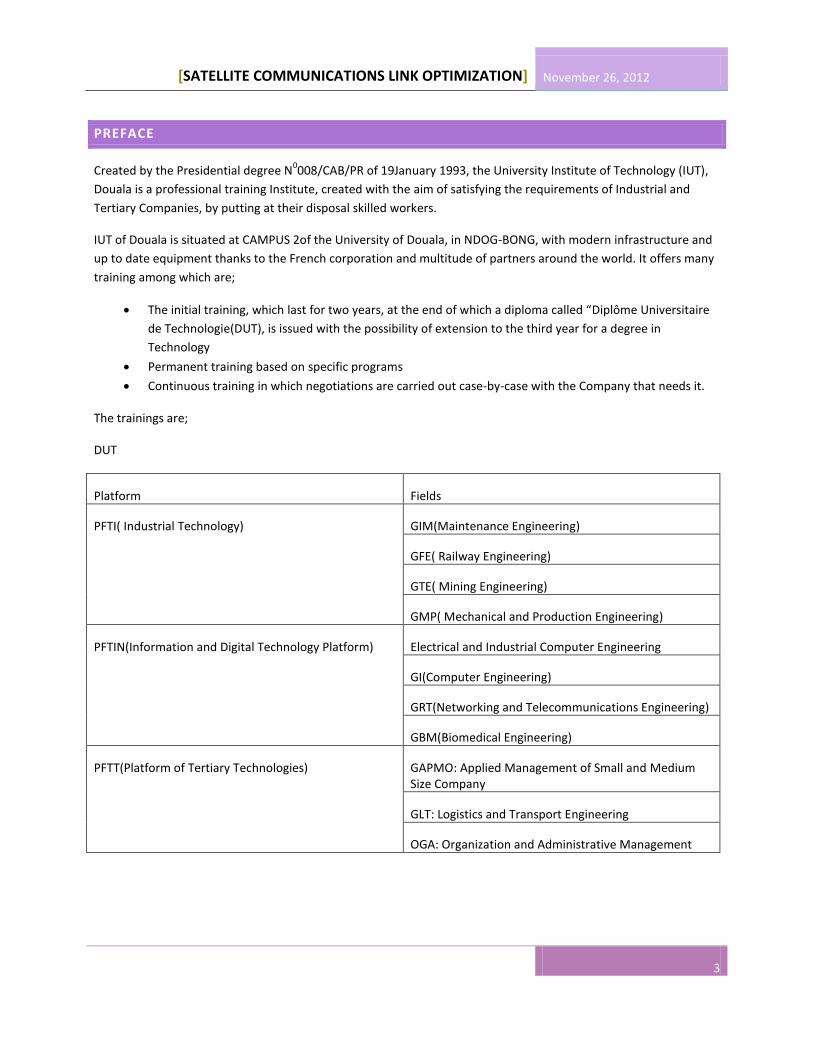
Created by the Presidential degree N0008/CAB/PR of 19January 1993, the University Institute of Technology (IUT),
Douala is a professional training Institute, created with the aim of satisfying the requirements of Industrial and
Tertiary Companies, by putting at their disposal skilled workers.
IUT of Douala is situated at CAMPUS 2of the University of Douala, in NDOG-BONG, with modern infrastructure and
up to date equipment thanks to the French corporation and multitude of partners around the world. It offers many
training among which are;
The initial training, which last for two years, at the end of which a diploma called “Diplôme Universitaire
de Technologie(DUT), is issued with the possibility of extension to the third year for a degree in
Technology
Permanent training based on specific programs
Continuous training in which negotiations are carried out case-by-case with the Company that needs it.
The trainings are;
DUT
Platform Fields
PFTI( Industrial Technology) GIM(Maintenance Engineering)
GFE( Railway Engineering)
GTE( Mining Engineering)
GMP( Mechanical and Production Engineering)
PFTIN(Information and Digital Technology Platform) Electrical and Industrial Computer Engineering
GI(Computer Engineering)
GRT(Networking and Telecommunications Engineering)
GBM(Biomedical Engineering)
PFTT(Platform of Tertiary Technologies) GAPMO: Applied Management of Small and Medium Size Company
GLT: Logistics and Transport Engineering
OGA: Organization and Administrative Management

November 26, 2012
SATELLITE COMMUNICATIONS LINK OPTIMIZATION
4
For BTS
ACO Commerce
CGE Enterprise Management Accounting
ET Electrotecnique
FM/CM Mechanical Manufacturing/ Mechanical Construction
II Industrial Computing
[SATELLITE COMMUNICATIONS LINK OPTIMIZATION] November 26, 2012
5
PROJECT SUMMARY
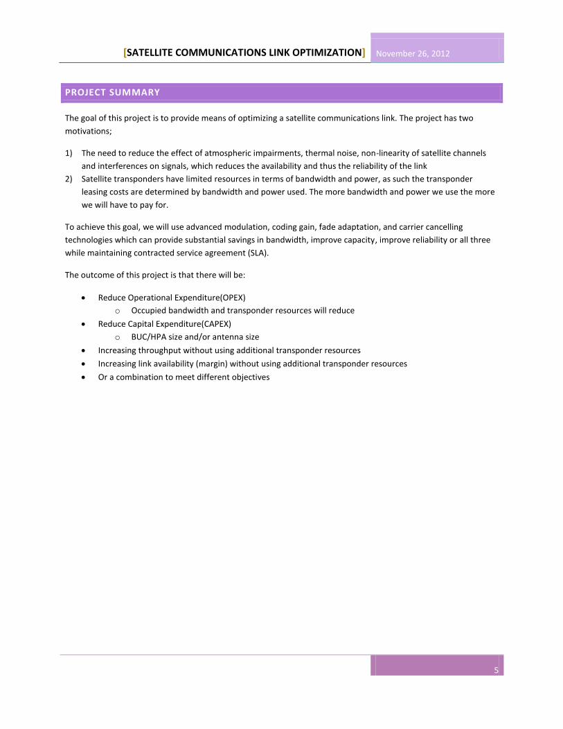
The goal of this project is to provide means of optimizing a satellite communications link. The project has two
motivations;
1) The need to reduce the effect of atmospheric impairments, thermal noise, non-linearity of satellite channels
and interferences on signals, which reduces the availability and thus the reliability of the link
2) Satellite transponders have limited resources in terms of bandwidth and power, as such the transponder
leasing costs are determined by bandwidth and power used. The more bandwidth and power we use the more
we will have to pay for.
To achieve this goal, we will use advanced modulation, coding gain, fade adaptation, and carrier cancelling
technologies which can provide substantial savings in bandwidth, improve capacity, improve reliability or all three
while maintaining contracted service agreement (SLA).
The outcome of this project is that there will be:
Reduce Operational Expenditure(OPEX)
o Occupied bandwidth and transponder resources will reduce
Reduce Capital Expenditure(CAPEX)
o BUC/HPA size and/or antenna size
Increasing throughput without using additional transponder resources
Increasing link availability (margin) without using additional transponder resources
Or a combination to meet different objectives
November 26, 2012
SATELLITE COMMUNICATIONS LINK OPTIMIZATION
6
ABSTRACT
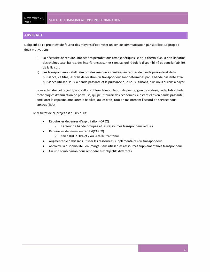
L'objectif de ce projet est de fournir des moyens d'optimiser un lien de communication par satellite. Le projet a
deux motivations;
i) La nécessité de réduire l'impact des pertubations atmosphériques, le bruit thermique, la non-linéarité
des chaînes satellitaires, des interférences sur les signaux, qui réduit la disponibilité et donc la fiabilité
de la liaison.
ii) Les transpondeurs satellitaire ont des ressources limitées en termes de bande passante et de la
puissance, ce titre, les frais de location du transpondeur sont déterminés par la bande passante et la
puissance utilisée. Plus la bande passante et la puissance que nous utilisons, plus nous aurons à payer.
Pour atteindre cet objectif, nous allons utiliser la modulation de pointe, gain de codage, l'adaptation fade
technologies d'annulation de porteuse, qui peut fournir des économies substantielles en bande passante,
améliorer la capacité, améliorer la fiabilité, ou les trois, tout en maintenant l'accord de services sous
contrat (SLA).
Le résultat de ce projet est qu'il y aura:
Réduire les dépenses d'exploitation (OPEX)
o Largeur de bande occupée et les ressources transpondeur réduira
Require les dépenses en capital(CAPEX)
o taille BUC / HPA et / ou la taille d'antenne
Augmenter le débit sans utiliser les ressources supplémentaires du transpondeur
Accroître la disponibilité lien (marge) sans utiliser les ressources supplémentaires transpondeur
Ou une combinaison pour répondre aux objectifs différents
[SATELLITE COMMUNICATIONS LINK OPTIMIZATION] November 26, 2012
7
TABLE OF CONTENTS
Preface ........................................................................................................................................................................... 3
project summary ............................................................................................................................................................ 5
Abstract .......................................................................................................................................................................... 6
acronyms ...................................................................................................................................................................... 12
General introduction .................................................................................................................................................... 16
part I satellite communications system overview ........................................................................................................ 17
CHAPTER 1: INTRODUCTION TO SATELLITE COMMUNICATIONS ................................................................................. 18
1.1 Definition and Early History ........................................................................................................................ 18
1.2 Basic Satellite Communication System Definition ...................................................................................... 20
1.2.1 The Space Segment ................................................................................................................................ 20
.1.2.2 The Ground Segment ............................................................................................................................. 21
1.3. Satellite Link Parameters ........................................................................................................................ 21
1.4 Satellite Orbits ............................................................................................................................................ 22
1.5 Radio Regulations ....................................................................................................................................... 22
1.6 Space Radiocommunications Services ........................................................................................................ 23
1.7 Frequency bands ......................................................................................................................................... 24
CHAPTER 2-SATELLITE ORBITS ...................................................................................................................................... 26
2.1 Kepler’s laws ............................................................................................................................................... 27
2.1.1 Kepler’s First Law .................................................................................................................................... 27
2.1.2 kepler’s second law ................................................................................................................................ 27
2.3 Kepler’s third law ........................................................................................................................................ 28
2.3 orbital parameters .......................................................................................................................................... 28
2.3 Orbits in common use ..................................................................................................................................... 29
2.3.1 Geostationary orbit .................................................................................................................................... 29

November 26, 2012
SATELLITE COMMUNICATIONS LINK OPTIMIZATION
8
2.3.2 Geosynchronous orbit ................................................................................................................................ 29
2.3.3 Low earth ORBIT (Leo) ................................................................................................................................ 30
2.3.4 Medium earth orbit .................................................................................................................................... 30
2.3.5 Highly elliptical orbit ................................................................................................................................... 30
2.3.6 Polar orbit ................................................................................................................................................... 30
2.3.7 Geometry of GSO Link ................................................................................................................................ 30
Chapter 3 – satellite subsystems .................................................................................................................................. 31
3.1 satellite bus ................................................................................................................................................. 33
3.1.1 Physical structure ........................................................................................................................................ 33
3.1.2 Power Subsystem ........................................................................................................................................ 34
3.1.3 Attitude control ........................................................................................................................................... 34
3.1.4 Orbital control ............................................................................................................................................. 35
3.1.5 Thermal Control .......................................................................................................................................... 35
3.1.6 Tracking, Telemetry, command and Monitoring ......................................................................................... 36
3.2 Satellite Payload ................................................................................................................................................. 37
3.2.1 Transponder ........................................................................................................................................... 37
3.2.1.1 frequency translation transponder .................................................................................................... 37
3.2.1.2 on-board processing transponder ..................................................................................................... 38
3.2.2 antennas ..................................................................................................................................................... 38
part II ............................................................................................................................................................................ 39
CHAPTER 4 noise .......................................................................................................................................................... 40
4.1 types of noise .............................................................................................................................................. 41
4.1.1 thermal noise ......................................................................................................................................... 42
4.2 interference ................................................................................................................................................ 43
4.3 intermodulation .......................................................................................................................................... 45
chapter 5- impairments ................................................................................................................................................ 45
[SATELLITE COMMUNICATIONS LINK OPTIMIZATION] November 26, 2012
9
5.1 signal attenuation ....................................................................................................................................... 46
5.1.1 rain attenuation...................................................................................................................................... 46
5.1.2 GASEOUS attenuation ............................................................................................................................ 47
5.1.3 cloud attenuation ................................................................................................................................... 47
5.1.4 snow and ice attenuation ............................................................................................................................ 47
5.2 signal path effect related to refraction .............................................................................................................. 48
5.2.1 Tropospheric scintillation ............................................................................................................................ 48
5.2.2 signal polarization effects ........................................................................................................................... 48
part III ........................................................................................................................................................................... 50
chapter modulation and coding .................................................................................................................................. 52
6.1 types of modulation ........................................................................................................................................... 52
6.1.1 types of phase shift keying modulation and bandwidth efficiency ............................................................. 53
6.1.2 power efficiency of the various schemes .................................................................................................... 54
6.1.3 power requirement of various schemes-eb/no vs BER ................................................................................ 55
6.2 CHANNEL encoding ............................................................................................................................................ 56
6.2.1 Block encoding and convolutional encoding ................................................................................................... 56
6.2.1a block encoding .......................................................................................................................................... 56
6.2.1b convolution encoding ................................................................................................................................ 56
6.2.2 concatenated encoding ............................................................................................................................... 57
6.2.3 Turbo codes ................................................................................................................................................. 57
6.2.4 Low Density Parity check CODES (LDPC) ..................................................................................................... 57
6.3 channel decoding ............................................................................................................................................... 57
6.4 power-bandwidth tradeoff ................................................................................................................................. 59
6.4.1 coding with variable bandwidth .................................................................................................................. 59
6.4.2 coding with constant bandwidth ................................................................................................................. 59
chapter 7 SATELLITE LINK Budget ................................................................................................................................ 60
November 26, 2012
SATELLITE COMMUNICATIONS LINK OPTIMIZATION
10
7.1 configuration of a link ........................................................................................................................................ 60
7.2 antenna parameters ........................................................................................................................................... 61
7.2.1 antenna gains .............................................................................................................................................. 61
7.2.2 radiation pattern and angular beamwidth .................................................................................................. 61
7.2.3 Polarization.................................................................................................................................................. 63
7.3 radiated power ................................................................................................................................................... 64
7.3.1 effective isotropic radiated power (EIRP) ................................................................................................... 64
7.3.2 power flux density ....................................................................................................................................... 64
7.4 Received signal power ........................................................................................................................................ 65
7.4.1 Power captured by the receiving antenna and free space path loss .......................................................... 65
7.5 additional losses ................................................................................................................................................. 66
7.5.1 attenuation in the atmosphere ................................................................................................................... 67
7.5.2 LOSSES IN THE TRANSMITTING AND RECEIVING EQUIPMENT .................................................................... 67
7.5.3 DEPOINTING LOSSES ................................................................................................................................... 68
7.5.4 losses due to polarization mismatch ........................................................................................................... 69
7.5.5 conclusion ................................................................................................................................................... 69
7.6 noise power spectral density at the receiver input ............................................................................................ 70
7.6.1 origin of noise .............................................................................................................................................. 70
7.6.2 Noise CHARACTERIZATION .......................................................................................................................... 70
7.6.3 noise temperature of a noise source .......................................................................................................... 70
7.6.4 noise figure .................................................................................................................................................. 70
7.6.5 EFFECTIVE INPUT NOISE TEMPERATURE OF AN ATTENUATOR ................................................................... 71
7.6.6 effective input noise temperature of cascaded elements .......................................................................... 71
7.6.7 EFFECTIVE INPUT NOISE TEMPERATURE OF A RECEIVER ............................................................................ 71
7.6.8 antenna noise temperature ........................................................................................................................ 72
7.6.8 noise temperature of a satellite antenna .................................................................................................... 72
[SATELLITE COMMUNICATIONS LINK OPTIMIZATION] November 26, 2012
11
7.6.9 noise temperature of an earth station ANTENNA (downlink) ..................................................................... 72
7.7 SYSTEM NOISE TEMPERATURE ........................................................................................................................... 73
7.7.1 conclusion ................................................................................................................................................... 74
7.8 individual link performance ................................................................................................................................ 75
7.8.1 carrier to noise power spectral density ratio at the receiver input ............................................................ 75
7.8.2 clear sky condition ....................................................................................................................................... 76
7.9 link performance under rain conditions ............................................................................................................. 80
7.9.1 uplink performance ..................................................................................................................................... 80
7.9.2 downlink performance ................................................................................................................................ 81
7.9.3 conclusion ................................................................................................................................................... 81
7.10 overall link performance with a transparent satellite ...................................................................................... 82
7.10.1 characteristics of the satellite channel ...................................................................................................... 82
7.10.2 satellite power flux density at saturation ................................................................................................. 83
7.10.3 satellite eirp at saturation ......................................................................................................................... 84
7.10.4 satellite repeater gain ............................................................................................................................... 84
7.10.5 input AND OUTPUT BACK-OFF .................................................................................................................. 84
7.10.6 carrier power at the satellite receiver input ............................................................................................. 85
7.10.7 expression for without interference from other systems or intermodulation............................... 85
7.10.8 expression for taking account of interference and intermodulation ............................................. 86
chapter 8 optimization ................................................................................................................................................. 87
8.1 link Margin.......................................................................................................................................................... 87
8.2 Power restoral techniques ................................................................................................................................. 88
8.2.1 beam diversity ................................................................................................................................................. 88
8.3 power control ..................................................................................................................................................... 89
8.3.1 uplink power control ................................................................................................................................... 89
8.4 site diversity ....................................................................................................................................................... 90

November 26, 2012
SATELLITE COMMUNICATIONS LINK OPTIMIZATION
12
8.5 signal modification techniques .......................................................................................................................... 91
8.5.1 Optimization By Doubletalk carrier-in-carrier ............................................................................................. 91
8.5.6 Double Talk Carrier-in-carrier cancellation process ........................................................................................ 93
8.6 adaptive coding and MODULATION (ACM) ........................................................................................................ 94
8.6.1 acm background .......................................................................................................................................... 95
8.6.2 requirements for ACM ................................................................................................................................ 96
9.0 general conclusion ................................................................................................................................................. 97
Bibliographic references .............................................................................................................................................. 97
ACRONYMS
ACI ADJACENT CHANNEL
INTERFERENCE
ES EARTH STATION
ADC ANALOG TO DIGITAL CONVERSION FDM FREQUENCY DIVISION MULTIPLEX
ADM ADAPTIVE DELTA MODULATION FEC FORWARD ERROR CORRECTION
ADPCM ADAPTIVE PULSE CODE
MODULATION
FES FIXED EARTH STATION
ALC AUTOMATIC LEVEL CONTROL FGM FIXED GAIN MODE
AM AMPLITUDE MODULATION FM FREQUENCY MODULATION
AMSS AERONAUTIC AL MOBILE SATELLITE
SERVICE
FSS FIXED SATELLITE SERVICES
APSK AMPLITUDE PHASE SHIFT KEYING GC GLOBAL COVERAGE

[SATELLITE COMMUNICATIONS LINK OPTIMIZATION] November 26, 2012
13
AR AXIAL RATIO GCS GROUND CONTROL STATION
BEP BIT ERROR PROBABILITY GEO GEOSTATIONARY EARTH ORBIT
BER BIT ERROR RATE GSO GEOSTATIONARY SATELLITE ORBIT
BPF BAND PASS FILTER HEO HIGHLY ELLIPTICAL ORBIT
BPSK BINARY PHASE SHIFT KEYING HIO HIGHLY INCLINED ORBIT
BS BASE STATION HPA HIGH POWER AMPLIFIER
BSS BROADCAST SATELLITE SERVICE HPB HALF POWER BANDWIDTH
BW BANDWIDTH IBO INPUT BACK-OFF
CAMP CHANNEL AMPLIFIER IF INTERMEDIATE FREQUENCY
CCI CO CHANNEL INTERFERENCE IMUX INPUT MULTIPLEX
CDMA CODE DIVISION MULTIPLE ACCESS INMARSAT INTERNATIONAL MARITIME SATELLITE
ORGANIZATION
D/C DOWN CONVERTER INTELSAT INTERNATIONAL TELECOMMUNICATIONS
SATELLITE CONSORTIUM
DA DEMAND ASSIGNMENT IOT IN ORBIT TEST
dB DECIBEL ISL INTER SATELLITE LINK
DE Differentially ENCODED ITU INTERNATIONAL TELECOMMUNICATIONS
UNION
DEMOD Demodulator

November 26, 2012
SATELLITE COMMUNICATIONS LINK OPTIMIZATION
14
EIRP EFFECTIVE ISOTROPIC RADIATED
POWER
LEO LOW EARTH ORBIT PLMN PUBLIC LAND MOBILE NETWORK
LHCP LEFT HAND CIRCULAR POLARIZATION
PM PHASE MODULATION
LNA LOW NOISE AMPLIFIER POL POLARIZATION
LNB LOW NOISE BLOCK PSK PHASE SHIFT KEYING
LO LOCAL OSCILLATOR PSTN PUBLIC SWITCHED TELEPHONE NETWORK
LPF LOW PASS FILTER PTN PUBLIC TELECOMMUNICATIONS NETWORK
MCPC MULTIPLE CHANNEL PER CARRIER PTO PUBLIC TELECOMMUNICATIONS OPERATOR
MEO MEDIUM EARTH ORBIT QoS QUALITY OF SERVICE
MES MOBILE EARTH STATION QPSK QUADRATURE PHASE SHIFT KEYING
MF MULTIFREQUENCY RF RADIO FREQUENCY
MOD MODULATOR RHCP RIGHT HAND CIRCULAR POLARIZATION
MODEM MODULATOR/DEMODULATOR RS REED SOLOMON(coding)
MSK MINIMUM SHIFT KEYING RX RECEIVER
MSS MOBILE SATELLITE SERVICE SC SUPPRESSED CARRIER
MUX MULTIPLEXER SCPC SINGLE CHANNEL PER CARRIER
MX MIXER SEP SYMBOL ERROR PROBABILITY
NASA NATIONAL AERONAUTIC AND SPACE ADMINISTRATION
SL SATELLITE
N-GSO NON-GEOSTATIONARY SATELLITE ORBIT
SNR SIGNAL-TO-NOISE RATIO
OBO OUTPUT BACK-OFF TWTA TRAVELING WAVE TUBE AMPLIFIER
OBP ON BOARD PROCESSING Tx TRANSMITTER
PCM PULSE CODE MODULATION VSAT VERY SMALL APERTURE TERMINAL
PCS PERSONAL COMMUNICATION SYSTEM
XPD CROSS POLARIZATION DISCRIMINATION

[SATELLITE COMMUNICATIONS LINK OPTIMIZATION] November 26, 2012
15
PDF PROBABILITY DENSITY FUNCTION XPI CROSS POLARIZATION ISOLATION
PLL PHASE LOCKED LOOP Xponder TRANSPONDER

November 26, 2012
SATELLITE COMMUNICATIONS LINK OPTIMIZATION
16
GENERAL INTRODUCTION
Since their introduction in the mid-1960s, satellite communications have grown from a futuristic experiment into an integral part of today’s “wired world.” Satellite communications are at the core of a global, automatically switched telephony network. Today’s communications satellite have extensive capabilities in applications involving data, voice and video with services provided to fixed, broadcast, mobile, personal communications and private users. But Satellite communication is highly affected by propagation impairments at the atmosphere, non-linearity of the satellite channel, Thermal noise, Interferences and also regulatory constraints. Therefore a good knowledge and modeling of the propagation channel is necessary for the performance assessment. This is thus a major preoccupation of most satellite operators.
The organization of the project (Dissertation) is as follows:
Part 1 describes a general overview of the satellite communication system in three chapters.
Part2 present a brief description of the impairments encountered in this domain in three chapters.
Part3 briefly talks on modulation and coding in one chapter. It also presents the parameters
necessary to calculate the performance of a link. It is concluded with the calculation of link
performance, for an uplink, a downlink and overall link from an uplink through a satellite to a
downlink.
Part4 presents the different means of optimizing a satellite link, in two parts. The first part, using
power restoral techniques and the second part using signal modification techniques.
[SATELLITE COMMUNICATIONS LINK OPTIMIZATION] November 26, 2012
17
PART I SATELLITE COMMUNICATIONS SYSTEM OVERVIEW

November 26, 2012
SATELLITE COMMUNICATIONS LINK OPTIMIZATION
18
CHAPTER 1: INTRODUCTION TO SATELLITE COMMUNICATIONS
1.1 DEFINITION AND EARLY HISTORY
A communications satellite is an orbiting artificial earth satellite that receives a communications signal from a
transmitting ground station, amplifies and possibly processes it, then transmits it back to the earth for reception by
one or more receiving ground stations. Communications information neither originates nor terminates at the
satellite itself. The satellite is an active transmission relay, similar in function to relay towers used in terrestrial
microwave communications.
The Commercial communication Satellite exists since the mid-1960s.Within a space of about 50years, it has grown
from an alternative technology to a mainstream transmission technology. Today’s communication satellites offer
extensive capabilities in applications involving data, voice and video, with services provided to fixed, broadcast,
mobile and personal communication and private network users
Communications Satellites offer advantages that are not readily available over alternative modes of transmissions
such as terrestrial microwave, cable or fiber optic networks, such as:
Distance Independent cost: The cost is the same, regardless of the distance between the transmitting and
the receiving earth stations.
Fixed Broadcast Cost: Broadcast from an earth station to a number of other earth station is independent
of the number of earth stations receiving the transmission.
High capacity: Capacity ranges from 10s of megabits to 100s of Mbps
Low error rate: Bit errors on a digital satellite link turns to be random, allowing statistical detection and
error correction techniques to be used. Error rates of one error in 106 bits and higher can be seen
commonly.
Diverse User Network. Due to its large coverage area, it can be used to interconnect land, sea and air
users who can be mobile or fixed

[SATELLITE COMMUNICATIONS LINK OPTIMIZATION] November 26, 2012
19
The idea of an artificial orbiting satellite capable of relaying communication to and from the earth is attributed to
Arthur C. Clarke. Below is a table with information concerning the early satellites, their launched dates, and basic
information concerning the satellites.
Satellite name Launched date Basic Function/use
SPUNIK1 1957 USSR
SCORE 1958 By USA Relayed a recorded voice message with delay
ECHO1 &2 1960 BY NASA
COURIER October 1960 First to employ solar cells for power
WESTFORD 1963 by US Army
Voice and frequency shift keying transmission.
TELSTAR 1&2 1962 and 1963 Multichannel telephone, telegraph, facsimile and television transmission
RELAY1 & 2 1962 and 1964 Extensive telephony and network television transmission between USA, Europe and Japan
SYNCOM2 & 3 1963 and 1964 First communication from a synchronous satellite
EARLY BIRD 1965 First commercial communication from a synchronous satellite.
Later called INTELSAT
ATS-1 1966 First multiple access communication from synchronous orbit
ATS-3 1967 Multiple access communication with Orbit Control
ATS-5 1969 Design to provide propagation data on the effect of the atmosphere on Earth-Space communication.
INTELSAT 1964 Created , becoming the recognized international legal entity satellite communication
Table1.1
These early accomplishments and events led to the rapid growth of the satellite communication’s industry,
beginning in the mid-1960s. INTELSAT was the prime mover in that time focusing on the benefits of satellite
communication to many nations
November 26, 2012
SATELLITE COMMUNICATIONS LINK OPTIMIZATION
20
1.2 BASIC SATELLITE COMMUNICATION SYSTEM DEFINITION
Satellite communications system is broken down into two main segments: the space segment and the ground (or
earth) segment.
1.2.1 THE SPACE SEGMENT
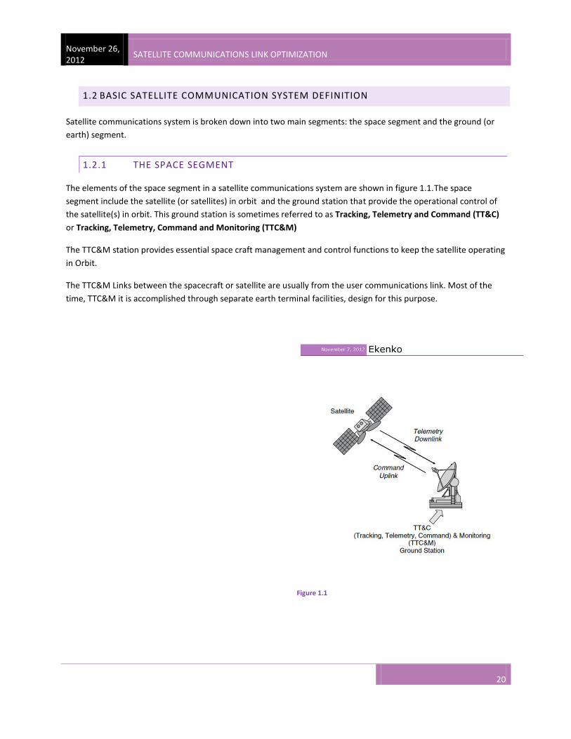
The elements of the space segment in a satellite communications system are shown in figure 1.1.The space
segment include the satellite (or satellites) in orbit and the ground station that provide the operational control of
the satellite(s) in orbit. This ground station is sometimes referred to as Tracking, Telemetry and Command (TT&C)
or Tracking, Telemetry, Command and Monitoring (TTC&M)
The TTC&M station provides essential space craft management and control functions to keep the satellite operating
in Orbit.
The TTC&M Links between the spacecraft or satellite are usually from the user communications link. Most of the
time, TTC&M it is accomplished through separate earth terminal facilities, design for this purpose.
Figure 1.1

[SATELLITE COMMUNICATIONS LINK OPTIMIZATION] November 26, 2012
21
.1.2.2 THE GROUND SEGMENT
It consists of the earth terminal(s) that make use of the communication capabilities of the space segment. It should be noted that the TTC&M do not make part of the ground segment.
The ground segment terminals could be one of the following:
Fixed Terminals
Transportable Terminals
Mobile Terminals
1.3. SATELLITE LINK PARAMETERS
Satellite communications link is defined by several parameters as shown in figure 1.2. These parameters are used in
the evaluation of a satellite communication link. The portion of the link from the earth station to the satellite is
called uplink, while the portion from the satellite to the ground station is called downlink. Either station in the
figure has an uplink and a downlink. The electronics in the satellites that receives the uplink signal, amplifies and
possibly processes the signal and then reformat and retransmit the signal back to the downlink is called the
transponder. It is indicated by the triangular symbol in the figure. The Antennas of the satellite that receives the
signal and transmit it on the downlink are not included as part of the transponder electronics. A channel is defined
as a one way link from A-to-S-to-B or from B-to-S-to-A. A duplex link from A-to-S-to-B and from B-to-S-to-A is called
a circuit. A Half-Circuit is the link from an earth
station to the satellite and back. That is A-to-S and S-
to-A is a half-circuit.

November 26, 2012
SATELLITE COMMUNICATIONS LINK OPTIMIZATION
22
1.4 SATELLITE ORBITS
A detail description of the satellite orbits will be given in chapter 2. We introduce here the four most commonly
used orbits, their altitudes and one way delay time. This information is given in table 1.2 below.
Satellite Orbit Orbital Altitude One-way delay
Geostationary Earth Orbit(GSO)
36000km 260ms
Low Earth Orbit(LEO) 160-640km 10ms
Medium Earth Orbit(MEO)
1600-4200km 100ms
High Earth Orbit(HEO) 40000km 10 to 260ms
table1
1.5 RADIO REGULATIONS
Radio Regulations are necessary to ensure an efficient use of the radio frequency spectrum by all communication
systems including terrestrial and satellite. This does not prevent each state from regulating its telecommunications
sector. All satellite operators must operate within the constraints of regulations related to fundamental parameters
and characteristics of the satellite communications system. The satellite communication parameters that are
regulated include the following;
Radiating frequency
Maximum allowable radiated power
Orbit Location(slot) for GSO
The purpose of the regulation is to minimize radio frequency interference and to some extent, physical interference
between systems. Potential radio interferences are not only from other satellite systems but also from other
terrestrial systems operating in the same frequency band. Two levels of regulations and allocation are involved in
the process: International and domestic. The primary organization responsible for international satellite
communication system regulation and allocation is the International Telecommunication Union (ITU), with
headquarters at Geneva, Switzerland.
ITU has three primary functions:
Allocation and Use of the radio- frequency spectrum;
Telecommunications standardization;
Development and expansion of the worldwide telecommunication

[SATELLITE COMMUNICATIONS LINK OPTIMIZATION] November 26, 2012
23
These functions are accomplished through the three sectors of the ITU organization: The Radiocommunications
Sector (ITU-R), responsible for the frequency allocations and use of the radio-frequency spectrum. The
Telecommunications Standard Sector (ITU-T), responsible for telecommunications standards and the
Telecommunications Development Sector (ITU-D), responsible for the development and expansion of the
worldwide telecommunications.
The International regulations developed by ITU are process by each country, where domestic level regulations are
developed. Each Country is left to manage and enforce the regulations within its boundaries.
In Cameroun this is managed by the Telecommunication Regulations Agency (ART).
1.6 SPACE RADIOCOMMUNICATIONS SERVICES
Two attributes determine the specific frequency band and other regulatory factors for a particular satellite system.
Service(s) to be provided by the particular satellite system/Network; and
The Location(s) of the satellite system ground terminals
Services applicable to satellite systems as designated by ITU are:
Aeronautical Mobile Satellite(AMSS)
Aeronautical Radionavigation Satellite(ARSS)
Amateur Satellite(ASS)
Broadcasting Satellite(BSS)
Earth-exploration Satellite(ESS)
Fixed Satellite(FSS)
Inter-satellite(ISS)
Land Mobile Satellite(LMSS)
Maritime Mobile Satellite(MMSS)
Maritime Radionavigation Satellite(MRSS)
Meteorological Satellite(MSS)
Mobile Satellite(MSS)
Radionavigation Satellite(RSS)
Space Operations(SOSS)
Space Research(SRSS)
Standard Frequency Satellite(SFSS)
Some of the service areas are divided into sub areas. For example the mobile satellite service (MSS) area is further
divided into Aeronautical Mobile Satellite Service (AMSS), Land Mobile Satellite Service (LMSS), and Maritime
Mobile Satellite Service (MMSS), with respect to the location of the ground terminals.

November 26, 2012
SATELLITE COMMUNICATIONS LINK OPTIMIZATION
24
The Location of the satellite system ground terminal, which is the second attribute, depends on the service region.
ITU divides the globe into three Telecommunications Service regions. Region1 consist of Europe and Africa,
Region2 the Americas, Region3 the Pacific Rim countries. Each of these regions is treated independently in terms of
frequency allocation. It is assumed that systems operating in one of these regions are protected from those in
another because of the geographical separation between them.
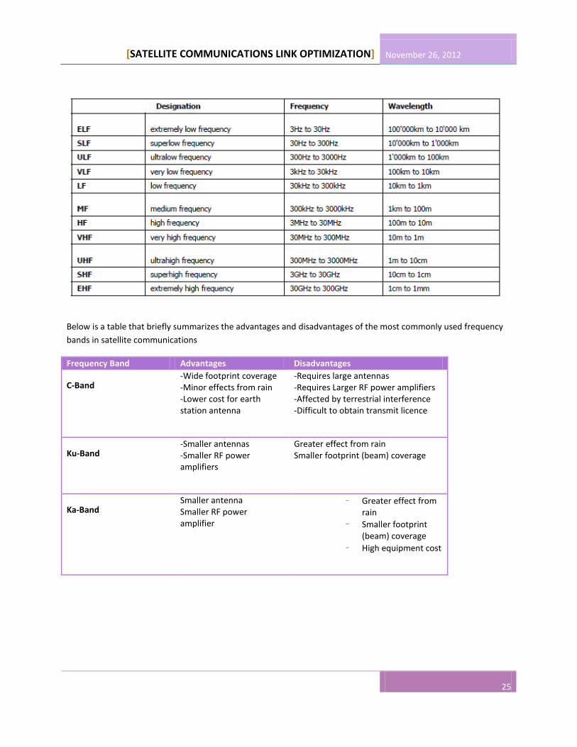
1.7 FREQUENCY BANDS
The frequency of operation is one of the major factors in the design and performance of a satellite communication
system. As it’s wavelength will determine the interaction effect of the atmosphere, and the resulting link
degradation. Two types of designations are used; The Letter Designation and the designation which divides the
spectrum from 3Hz to 300GHz. These are shown in the tables below
[SATELLITE COMMUNICATIONS LINK OPTIMIZATION] November 26, 2012
25
Below is a table that briefly summarizes the advantages and disadvantages of the most commonly used frequency
bands in satellite communications
Frequency Band Advantages Disadvantages
C-Band -Wide footprint coverage -Minor effects from rain -Lower cost for earth station antenna
-Requires large antennas -Requires Larger RF power amplifiers -Affected by terrestrial interference -Difficult to obtain transmit licence
Ku-Band -Smaller antennas -Smaller RF power amplifiers
Greater effect from rain Smaller footprint (beam) coverage
Ka-Band Smaller antenna Smaller RF power amplifier
– Greater effect from rain
– Smaller footprint (beam) coverage
– High equipment cost

November 26, 2012
SATELLITE COMMUNICATIONS LINK OPTIMIZATION
26
CHAPTER 2-SATELLITE ORBITS
The same laws of motion that governs the movement of the planets
around sun also control the movement of artificial satellites around the
earth .Satellite Orbital determination is based on the laws of motion
developed by Kepler and later refined by newton.
Competing forces act on the satellite; gravity turns to pull the satellite in
towards the earth, while its orbital velocity turns to pull the satellite away
from the earth. These forces are shown in figure 2.1
The gravitational force, Fin and the angular velocity, Fout , can be
represented as
Fin= m (
) ….2.1
and Fout=m (
)….2.2
where m=the satellite
mass, v= the satellite
velocity in the plane of
its orbit, r=orbital radius
(distance from the
center of the earth);
and =Kepler’s constant
(Geocentric
gravitational constant)
=3.9864002x Km3/s2.
If the gravitational force
from the sun, moon and other bodies are neglected, then
Fin=Fout and the velocity necessary to keep the satellite in orbit
will be
V= (√
) …..2.3
The orbital locations of
the spacecraft in a
communications
satellite system play a
major role in
determining the
coverage and
operational
characteristics of the
services provided by
that system. This
chapter describes the
general characteristics
of satellite orbits and
summarizes the
characteristics of the
most popular orbits for
communications
applications.
[SATELLITE COMMUNICATIONS LINK OPTIMIZATION] November 26, 2012
27
2.1 KEPLER’S LAWS
The laws of Kepler apply to any two bodies in space that interact through gravitation.
2.1.1 KEPLER’S FIRST LAW
Kepler’s first law as applied to artificial satellite orbits goes thus; the path followed by a satellite around the earth
will be an ellipse, with the center of mass of the earth as one of the two foci of the ellipse.
If no other forces are acting on the satellite, either intentionally by orbit control or unintentionally as in gravity
forces from other bodies, the satellite will eventually settle in an elliptical orbit, with the earth as one of the foci of
the ellipse. The size of the ellipse will depend on the satellite mass and its angular velocity.
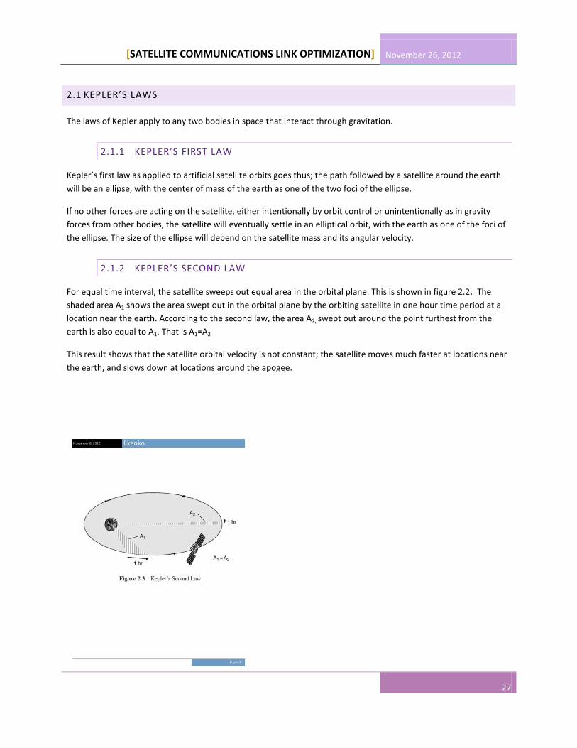
2.1.2 KEPLER’S SECOND LAW
For equal time interval, the satellite sweeps out equal area in the orbital plane. This is shown in figure 2.2. The
shaded area A1 shows the area swept out in the orbital plane by the orbiting satellite in one hour time period at a
location near the earth. According to the second law, the area A2, swept out around the point furthest from the
earth is also equal to A1. That is A1=A2
This result shows that the satellite orbital velocity is not constant; the satellite moves much faster at locations near
the earth, and slows down at locations around the apogee.
November 26, 2012
SATELLITE COMMUNICATIONS LINK OPTIMIZATION
28
2.3 KEPLER’S THIRD LAW
The square of the periodic time of orbit is proportional to the cube of the mean distance between the two bodies.
That is T2= [
]a
3, where T=orbital period in seconds s, a= distance between the bodies in km and µ=Kepler’s
constant=3.986004x10⁵km
3/s
2
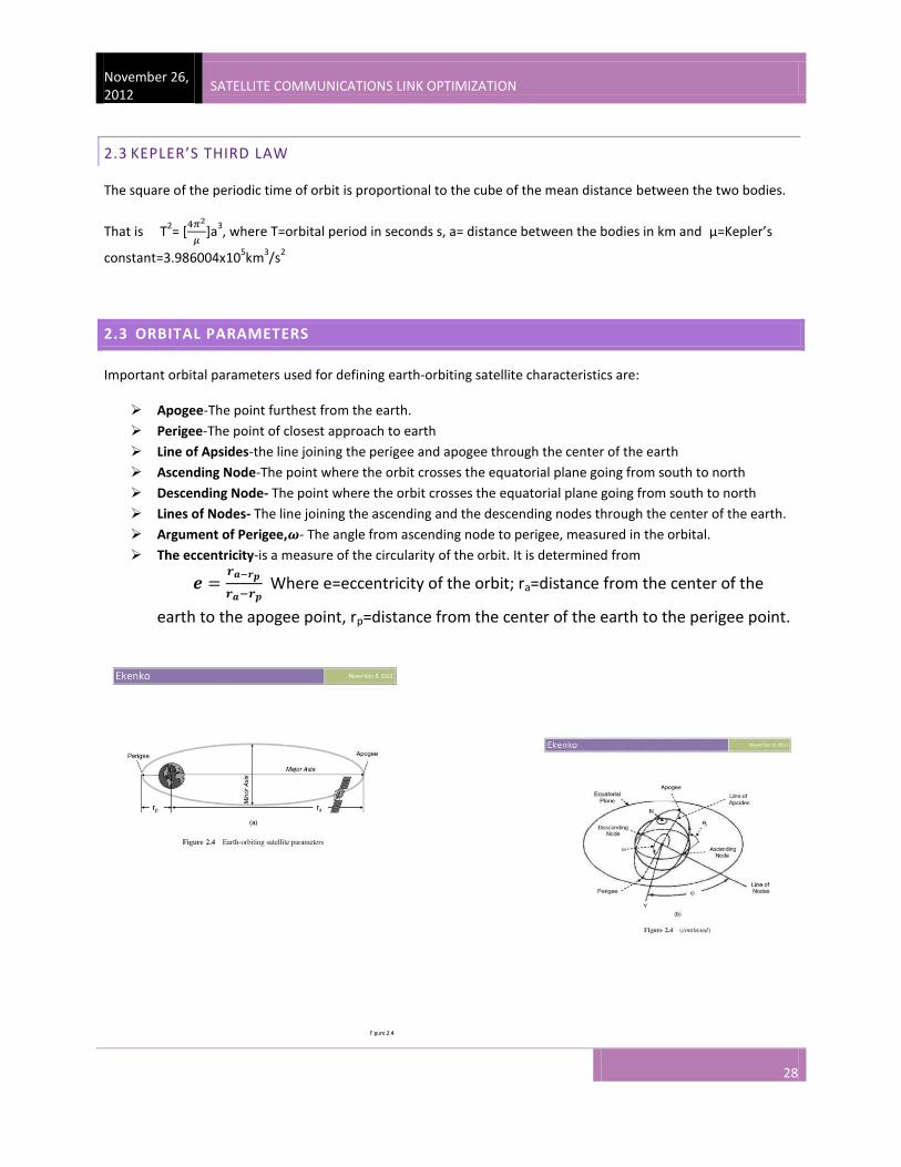
2.3 ORBITAL PARAMETERS
Important orbital parameters used for defining earth-orbiting satellite characteristics are:
Apogee-The point furthest from the earth.
Perigee-The point of closest approach to earth
Line of Apsides-the line joining the perigee and apogee through the center of the earth
Ascending Node-The point where the orbit crosses the equatorial plane going from south to north
Descending Node- The point where the orbit crosses the equatorial plane going from south to north
Lines of Nodes- The line joining the ascending and the descending nodes through the center of the earth.
Argument of Perigee, - The angle from ascending node to perigee, measured in the orbital.
The eccentricity-is a measure of the circularity of the orbit. It is determined from
Where e=eccentricity of the orbit; ra=distance from the center of the
earth to the apogee point, rp=distance from the center of the earth to the perigee point.
[SATELLITE COMMUNICATIONS LINK OPTIMIZATION] November 26, 2012
29
A circular orbit is a special case of an ellipse with equal major and minor axes (e=o)
That is for Elliptical orbit 0 < e < 1 and for Circular Orbit e = 0.
Inclination Angle is the angle between the orbital plane and the earth’s equatorial plane.
A satellite that is in an orbit with some inclination angle is said to be in an Inclined Orbit. A satellite that is in orbit
in the equatorial plane (inclination angle = 0) is in an Equatorial Orbit. A satellite in an orbit with inclination angle of
is said to be in a polar orbit.
All these orbits may be circular or elliptical depending on the orbital velocity and the direction of motion imparted
to the satellite on insertion into orbit. An orbit in which the satellite moves in the same direction as the earth’s
rotation is called a Prograde orbit, inclination angle 0 < < 90. A satellite in a retrograde orbit moves in the
opposite direction to earth rotation, inclination angle 90 < < 180
Most satellites are launched in Prograde orbit because the earth’s rotational velocity enhances the satellite orbital
velocity, reducing the amount of energy required to launch and place the satellite in orbit.
2.3 ORBITS IN COMMON USE
2.3.1 GEOSTATIONARY ORBIT
Kepler’s third law shows that there is a fixed relationship between orbit radius and the period of revolution of the
satellite. If we carefully choose an orbit radius we can determine the orbit period.
If an orbit radius is chosen so that the period of revolution of the satellite is exactly set to the period of rotation of
the earth. Also if the orbit is circular (e = 0) and the orbit is in the equatorial plane ( =0), the satellite will appear to
hover motionless above the earth. This orbit is called Geostationary Earth Orbit (GEO). This orbit radius is
42104Km. The GEO is an ideal orbit that cannot be achieved for real artificial satellites because there are many
other forces acting on the satellite apart of the earth gravity. In addition to this, extensive station keeping and a
vast amount of fuel is necessary to maintain the satellite in this orbit.
2.3.2 GEOSYNCHRONOUS ORBIT
It is one whose inclination angle is slightly greater than zero and possibly with an eccentricity above zero. It’s at an
altitude of 36000Km. Most current communications satellites operate in geosynchronous orbit.
Advantages -It’s the most common orbit -Fixed slant path -little or no ground station tracking required -2 to 3 satellites for global coverage (accept at the poles) -period of revolution is 23hours, 56minutes Disadvantages -Large path loss and significant latency (approximately 260ms for a duplex communication) -cannot provide coverage to high latitude locations Coverage can be increase by using high elevation angle but this produces problems such as increase ground station antenna tracking, which increases cost and system complexity.
November 26, 2012
SATELLITE COMMUNICATIONS LINK OPTIMIZATION
30
2.3.3 LOW EARTH ORBIT (LEO)
Operate typically at an altitude from 160 – 2400Km and is near circular. Requires earth tracking terminals, for continuous service. Advantages -Shorter earth – satellite link, leading to lower path loss as such smaller power and smaller antenna systems -can cover high latitude locations -the satellite is much smaller in size, as such requires less energy to put it in orbit Disadvantages -A constellation of multiple LEO (12, 24, 66 etc.) to provide global coverage -approximately 8 to 10 minutes per pass of an earth terminal -Requires earth antenna tracking -Oblateness or non-spherical nature of the earth causes major perturbations to LEO obit.
2.3.4 MEDIUM EARTH ORBIT
It is situated at an altitude from 10,000 to 20,000Km similar to LEO, but higher circular orbit.
One to two hours per pass for an earth terminal
Requires a constellation of satellite to provide global coverage, for example GPS requires up to 24 satellites.
It is mostly used for meteorological, remote sensing and position location application
2.3.5 HIGHLY ELLIPTICAL ORBIT
Popular for high latitude or polar coverage
Often referred to as MOLNIYA orbit
Eight to ten hour per pass for an earth terminal
Typical MOLNIYA orbit has a perigee altitude of 1000Km and an apogee altitude of nearly 40,000Km.
2.3.6 POLAR ORBIT
Circular orbit with an inclination near
Useful for sensing and data gathering services
2.3.7 GEOMETRY OF GSO LINK
GSO is the dominant orbit in use for communication satellites. Three key parameters of the GSO orbit are used for
evaluation of satellite link performance.
(distance) from the earth(Earth Station) to the satellite, in KM
from the earth station to the satellite in degrees
from the earth station to the satellite in degrees

[SATELLITE COMMUNICATIONS LINK OPTIMIZATION] November 26, 2012
31
Azimuth and elevation angle are called the look angle of
the earth station to the satellite. This is shown in figure
2.5
Input parameters that can be used with software tools
for determining the look angle are:
-
-
-Le=Earth Station Latitude
-Ls=Satellite latitude
There are also software tools which require just the
Country, name of the town and antenna size to find the
look angle
CHAPTER 3 – SATELLITE SUBSYSTEMS
A basic satellite system consists of a satellite (satellites) in space, relaying information between two or more users
through ground terminals and the satellite. The information relayed may be voice, data, video or a combination of
the three. The satellite is control from the ground through a satellite control facility, often called the Master
Control Center (MCC), which provide tracking, telemetry, command and monitoring for the system.
The Space Segment of the satellite system consist of the orbiting satellite (or satellites) and the ground satellite
control facilities necessary to keep the satellite(s) operational.
The Ground Segment or Earth Segment of the satellite system, consist of the transmit and receive earth stations
and the associated equipment to interface with the user network, as shown in figure 3.1
We will focus on the space segment of a general communication satellite
The Space segment equipment on-board the satellite can be divided into: BUS and
PAYLOAD.
-BUS: It refers to the basic satellite structure and the subsystem that supports the
satellite.

November 26, 2012
SATELLITE COMMUNICATIONS LINK OPTIMIZATION
32
The BUS subsystems are: Physical Structure,
Power Subsystem, Attitude and Orbital
Control subsystems, command and
telemetry subsystem.
-PAYLOAD: It is the equipment that provide
the service or services intended for the
satellite
A communication payload can be further
divided into Transponder and antenna
subsystems as shown in figure 3.2
A satellite may have more than one payload
[SATELLITE COMMUNICATIONS LINK OPTIMIZATION] November 26, 2012
33
3.1 SATELLITE BUS
The basic characteristics of a BUS subsystem are described below.
3.1.1 PHYSICAL STRUCTURE
It contains the other components of the satellite.
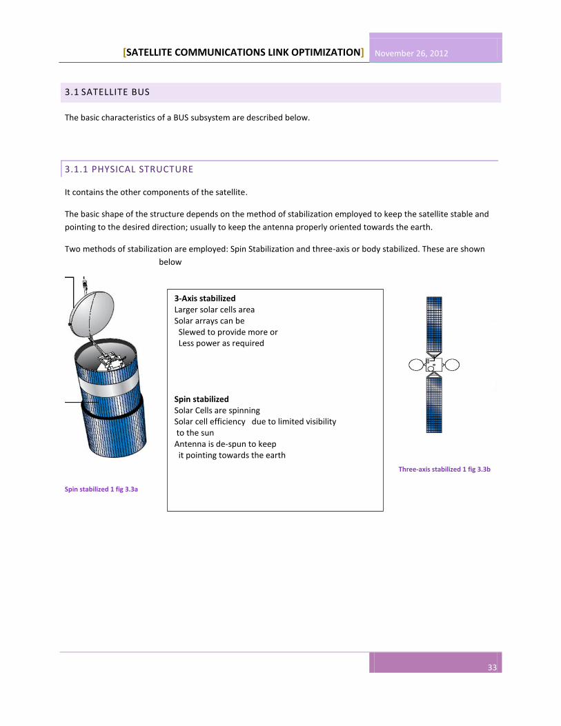
The basic shape of the structure depends on the method of stabilization employed to keep the satellite stable and
pointing to the desired direction; usually to keep the antenna properly oriented towards the earth.
Two methods of stabilization are employed: Spin Stabilization and three-axis or body stabilized. These are shown
below
Spin stabilized 1 fig 3.3a
Three-axis stabilized 1 fig 3.3b
3-Axis stabilized Larger solar cells area Solar arrays can be Slewed to provide more or Less power as required Spin stabilized Solar Cells are spinning Solar cell efficiency due to limited visibility to the sun Antenna is de-spun to keep it pointing towards the earth

November 26, 2012
SATELLITE COMMUNICATIONS LINK OPTIMIZATION
34
3.1.2 POWER SUBSYSTEM
The electrical power for operating equipment on a communication satellite is obtained
primarily from solar cells, which convert incident sunlight into electrical energy. Solar
cells operate at an efficiency of at the Beginning of Life (BOL) and can degrade
to at the End of Life (EOL), usually considered to be 15years. In addition large
number of cells connected in serial-parallel arrays, are required to support the
communication satellite electronic system.
t Two types of batteries:
t Specific energy density Nickel - cadmium: 25 - 30 W.hr/Kg
Nickel - Hydrogen: 25 - 60 W.hr/Kg
GEO LEO
t Depth of discharge (DOD) Nickel - cadmium 50% 10-20%
Nickel – hydrogen 70% 40-50%
3.1.3 ATTITUDE CONTROL
The attitude of a satellite refers to the orientation in space with respect to the earth. It helps the narrow directional
beam antenna to be pointed correctly to earth. Several forces can interact to affect the attitude of a spacecraft.
These forces are gravitational forces from the sun, moon and planet, solar pressure acting on the spacecraft body,
antenna and solar panels, earth’s gravitational field force.

[SATELLITE COMMUNICATIONS LINK OPTIMIZATION] November 26, 2012
35
The orientation is monitored on the spacecraft by Infrared Horizon Detectors. Four detectors are used to establish
a reference point; usually the center of the earth and any shift in orientation is detected by one or more of the
sensors. A control signal is generated that is used to activate attitude control devices to restore proper orientation.
Gas jets, ion thrusters and momentum wheels are used to provide active attitude control on communications
satellites. Since the earth is not a perfect sphere, the satellite will be accelerated towards one of the “stable” points
in the equatorial plane. This locations are and . In the absence of orbital control, the satellite will drift
and settle in one of these stable locations.
3.1.4 ORBITAL CONTROL
Orbital Control often referred to as Station Keeping, is the process required to maintain the satellite in its proper
orbit location. It is similar to though not the same as attitude control. GSO satellites will undergo forces that will
cause the satellite to drift in the East-West (longitude) direction and the North-South (Latitude) direction. Orbital
Control is usually maintained using Gas jets, Ion thrusters and momentum wheels.
The non-spherical properties of the earth primarily exhibited as an equatorial bulge, cause the satellite to drift
slowly in longitude along the equatorial plane. Control jets are pulsed to impart an opposite velocity component to
the satellite, causing the satellite to drift back to its nominal position. This is called East-West Station Keeping
Maneuvers, which are accomplished every two to three weeks.
North-South Station Keeping requires more fuel than East-West Station Keeping and often satellites are maintain
with little or no North-South station keeping, to extend on-orbit life.
The quantity of fuel that must be carried on-board the satellite to provide orbital and attitude control is usually a
determinant factor in the on-orbit life of a communication satellite.
3.1.5 THERMAL CONTROL
Thermal radiation from the sun heats on one side of the spacecraft, while the side facing the outer space is exposed
to extremely low temperature of space. Most of the equipment in the satellite itself generates heat, which must be
controlled.
Satellite thermal control is design to control the large thermal gradient generated in the satellite by removing or
relocating the heat to provide as stable as possible temperature environment for the satellite.
-Thermal Blankets and Thermal Shield are placed at critical locations to provide insulation. Radiation Mirrors are
placed around electronic subsystems, to protect critical equipment. Heat Pumps are used to relocate heat from
power devices such as Traveling Wave Tube Amplifiers (TWTA) to outer walls or heat sinks. Thermal heaters can
also be used to maintain adequate temperature conditions for some components, such as propulsion lines or
thrusters, where low temperature would cause severe problems.
Satellite antennas are highly affected by the heat from the sun. Large aperture antenna can be twisted.

November 26, 2012
SATELLITE COMMUNICATIONS LINK OPTIMIZATION
36
3.1.6 TRACKING, TELEMETRY, COMMAND AND MONITORING
Tracking, Telemetry, Command and Monitoring (TTC&M) provide essential spacecraft management and control
functions to keep the satellite operating safely in orbit.
The TTC&M links between the spacecraft and the ground are usually separated from the communications system
links. TTC&M links may operate in the same frequency bands or different frequency bands as the communications
links. Separate earth terminal facilities specifically design for the complex operation required to maintain the
spacecraft in orbit are used. A single TTC&M facility may maintain several spacecraft simultaneously in orbit
through TTC&M links to each vehicle. Figure 3.4 shows typical TTC&M facility elements.
TTC&M is divided into the satellite TTC&M subsystem and
the earth TTC&M subsystem.
The satellite TTC&M subsystem comprises the antenna,
command receiver, tracking and telemetry transmitter,
and possibly tracking sensors.
Telemetry data are received from the other subsystems of
the spacecraft, such as the payload, power, attitude and
thermal control.
Command data are relayed from the command receiver
to the other subsystems to control such parameters as
antenna pointing, transponder modes of operation,
battery and solar cell charges etc.
The ground TTC&M subsystem comprise the antenna,
telemetry receiver, command transmitter, tracking
subsystem and associated processing and analysis
functions
Satellite control and monitoring is accomplished through
monitors and keyboard interface. Major operations of
TTC&M are automated, with minimal human interface
required.
Tracking refers to the determination of the current orbital position and the movement of the spacecraft.
Telemetry involves the collection of data from sensors on-board the spacecraft and relay of this information to the
ground. Command is the complementary function of telemetry. The command systems relay specific control and
operations information from ground to the spacecraft, most often in response to telemetry.
[SATELLITE COMMUNICATIONS LINK OPTIMIZATION] November 26, 2012
37
3.2 SATELLITE PAYLOAD
A communications satellite payload is made up of two subsystems: Transponder and Antenna subsystems
3.2.1 TRANSPONDER
The Transponder in a communications satellite is the series of components that provide the communications
channel or link between the uplink signal received at the uplink antenna and the downlink signal transmitted at the
downlink antenna. A typical communications satellite will contain more than one transponder and some of the
equipment may be common to more than one transponder.
Each transponder generally operate in a different frequency band, with the allocated frequency band divided into
slots (sub bands), with a specified center frequency and operating bandwidth. For example a 500MHz frequency
band allocated for FSS can be divided among 12 transponders each of 36MHz bandwidth, width 4MHz guard band
between each. Typical commercial communications satellites can have 24 to 48 transponders.
The number of transponders can be doubled by the use of polarization frequency reuse. We can also spatial
separation of the signal in the form of narrow spot beam, which allow the reuse of the same carrier in spatially
separated locations on earth.
Communications satellite transponders can be implemented in two general types; Frequency Translation and On-
Board Processing Transponder.
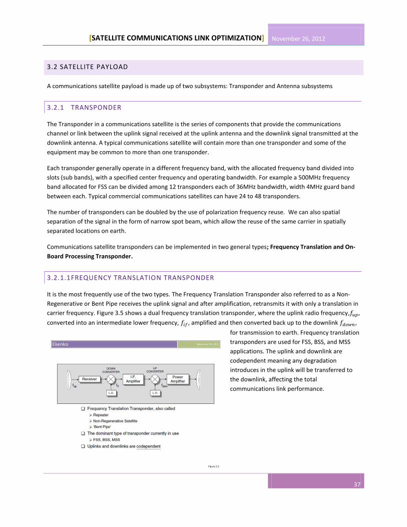
3.2.1.1 FREQUENCY TRANSLATION TRANSPONDER
It is the most frequently use of the two types. The Frequency Translation Transponder also referred to as a Non-
Regenerative or Bent Pipe receives the uplink signal and after amplification, retransmits it with only a translation in
carrier frequency. Figure 3.5 shows a dual frequency translation transponder, where the uplink radio frequency, ,
converted into an intermediate lower frequency, , amplified and then converted back up to the downlink ,
for transmission to earth. Frequency translation
transponders are used for FSS, BSS, and MSS
applications. The uplink and downlink are
codependent meaning any degradation
introduces in the uplink will be transferred to
the downlink, affecting the total
communications link performance.

November 26, 2012
SATELLITE COMMUNICATIONS LINK OPTIMIZATION
38
3.2.1.2 ON-BOARD PROCESSING TRANSPONDER
The On-Board processing transponder also called a Regenerative Repeater or Demo/Remod transponder or Smart
Satellite is shown in figure 3.6
The uplink signals at is demodulated to baseband, . The baseband signal is then available for
processing on-board, including reformatting and error correction. The baseband information is then remodulated
to the downlink carrier at , possibly in a different modulation format to the uplink and after final
amplification is transmitted to the downlink. The Demodulation/Remodulation process removes the uplink noise
and interference from the downlink, while allowing additional on board processing to be accomplished. Thus the
uplink and downlink are independent with respect to the evaluation of the overall link performance
This type of satellite turns to be more expensive than frequency translation satellites, but do offer significant
performance advantages.
Travelling wave tube amplifiers (TWTA) or Solid State Power Amplifiers (SSPA) are used to provide final output
amplification for each transponder channel.
3.2.2 ANTENNAS
The antenna system is a critical part of the satellite communications system, because it is an essential element in
increasing the strength of the transmitted or received signal to allow amplification, processing and eventual
retransmission. The most important parameters that define the performance of an antenna are; antenna gain,
antenna beamwidth, and antenna side lobes.
The gain defines the increased in strength achieved in concentrating the radio wave energy. The beamwidth
usually express as 3-dB beamwidth or half power beamwidth is a measure of the angle over which the maximum
gain occurs. The sidelobe is defined as the amount of gain in the off-axis direction. The common types of antennas
used in satellite communications are: Linear dipole, horn antenna, parabolic reflector and array antenna.

[SATELLITE COMMUNICATIONS LINK OPTIMIZATION] November 26, 2012
39
PART II
NOISE AND IMPAIRMENTS ARE THE MAJOR SOURCES OF DEGRADATION ON A SATELLITE COMMUNICATIONS
LINK. THIS PART PRESENTS ALL THE TYPES OF NOISE AND IMPAIRMENTS THAT CAN BE ENCOUNTERED ON A
COMMUNICATION LINK. A GOOD KNOWLEDGE OF THIS NOISE AND IMPAIRMENTS WILL HELP AN OPERATOR
BETTER OPTIMIZE PERFORMANCE.
THIS PART IS DIVIDED INTO TWO MAIN CHAPTERS. CHAPTER FOUR PRESENTS ALL THE NOISE ON A SYSTEM
WHILE CHAPTER FIVE PRESENTS THE IMPAIRMENTS.
PART ∥ NOISE AND IMPAIRMENTS
ON SATELLITE COMMUNICATIONS
LINK

November 26, 2012
SATELLITE COMMUNICATIONS LINK OPTIMIZATION
40
CHAPTER 4 NOISE
The figure 4.1 below shows the path taken by a signal from the transmitter to the receiver and the level of noise
present in the signal.
From the graph it can be seen that signal power and noise power are almost equal at the input of the receive
terminal. That is it is possible to confuse noise and carrier power.
At can also be seen that from the point the noise is injected into the signal, it follows the same path as the signal
and therefore goes through the same attenuation and gain stages
Noise can be introduced into a communication link at various points
At the transmit terminal
At the receive system of the satellite
In the satellite non-linear amplifier
At the transmit system of the satellite
At the receive terminal of the earth station.

[SATELLITE COMMUNICATIONS LINK OPTIMIZATION] November 26, 2012
41
4.1 TYPES OF NOISE
The following (figure4.2) are the major types of noise experienced in a satellite communication link
– Thermal Noise
In the satellite receive system
In the receive system of the earth terminal
– Interference
From the carriers in the same transponder
From carriers in other transponders in the same satellite
From other carriers in other satellites
– Intermodulation Noise
In the High Power Amplifier(HPA) of the transmit terminal
In the satellite High Power Amplifier(HPA)
November 26, 2012
SATELLITE COMMUNICATIONS LINK OPTIMIZATION
42
4.1.1 THERMAL NOISE
Every object in the universe generates thermal noise. Thermal noise is very weak, so it is important only when the
signal itself is very weak, that is at the input of the receive system of the satellite or the receive system of the
receive earth station.
Thermal noise is measured in terms of noise temperature “T”. The gain (G) to noise temperature (T) ratio of a
receive system, G/T is a key performance parameter of the receive system.
We can group thermal noise into Uplink Thermal Noise (satellite receive system) and Downlink Thermal Noise
(Terminal Receive System)
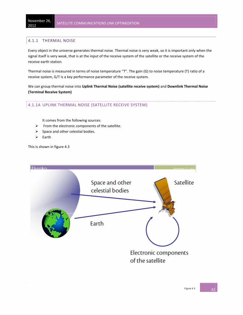
4.1.1A UPLINK THERMAL NOISE (SATELLITE RECEIVE SYSTEM)
It comes from the following sources:
From the electronic components of the satellite.
Space and other celestial bodies.
Earth
This is shown in figure 4.3
[SATELLITE COMMUNICATIONS LINK OPTIMIZATION] November 26, 2012
43
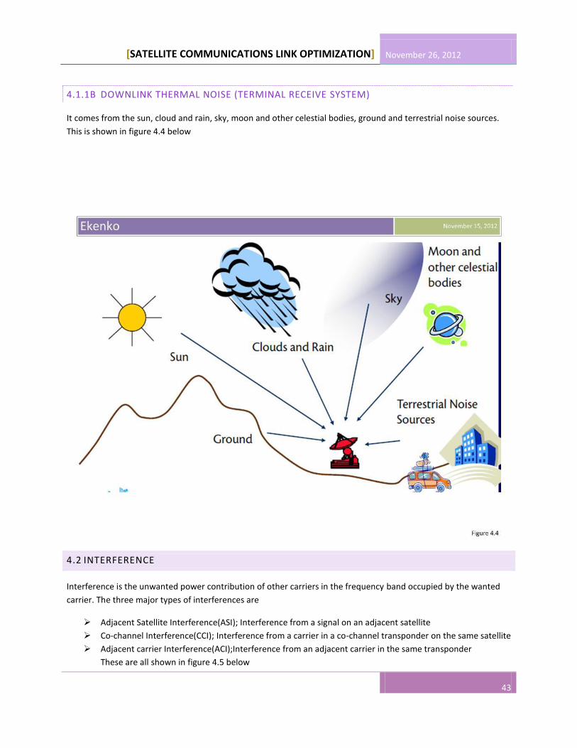
4.1.1B DOWNLINK THERMAL NOISE (TERMINAL RECEIVE SYSTEM)
It comes from the sun, cloud and rain, sky, moon and other celestial bodies, ground and terrestrial noise sources.
This is shown in figure 4.4 below
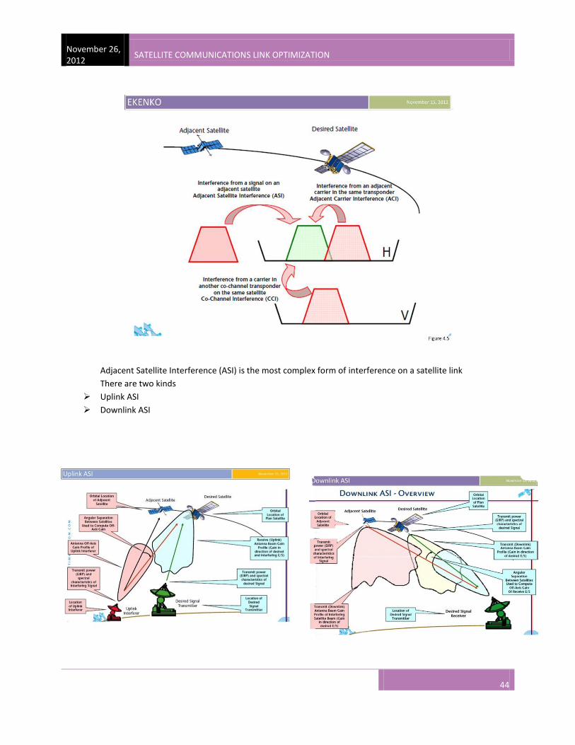
4.2 INTERFERENCE
Interference is the unwanted power contribution of other carriers in the frequency band occupied by the wanted
carrier. The three major types of interferences are
Adjacent Satellite Interference(ASI); Interference from a signal on an adjacent satellite
Co-channel Interference(CCI); Interference from a carrier in a co-channel transponder on the same satellite
Adjacent carrier Interference(ACI);Interference from an adjacent carrier in the same transponder
These are all shown in figure 4.5 below
November 26, 2012
SATELLITE COMMUNICATIONS LINK OPTIMIZATION
44
Adjacent Satellite Interference (ASI) is the most complex form of interference on a satellite link
There are two kinds
Uplink ASI
Downlink ASI

[SATELLITE COMMUNICATIONS LINK OPTIMIZATION] November 26, 2012
45
4.3 INTERMODULATION
Non-linear devices such as Traveling Wave Tube Amplifiers (TWTA) Or Solid State Power Amplifiers (SSPA) at the
satellite transponders or any High Power Amplifier (HPA) at the transmit terminal will generate intermodulation
noise when multiple carriers pass through them. The nature of the intermodulation noise depends on the carriers
and the non-linear device.
A precise computation of intermodulation noise is vital in predicting the performance close to saturation, for
maximum output performance.
CHAPTER 5- IMPAIRMENTS
The atmosphere offers an RF window for satellite communications.
At low frequencies the ionosphere cannot be penetrated by radio waves and acts as a reflector
At high frequencies the atmospheric gases absorb and severely attenuate the radio waves

November 26, 2012
SATELLITE COMMUNICATIONS LINK OPTIMIZATION
46
Propagation impairment at frequencies above 1GHz can be group into the following classes
Signal attenuation due to
o Atmospheric gases-primarily oxygen and water vapor
o Rain and snow
o Clouds
Signal polarization effects
o Depolarization due to rain
o Faradays rotation
Signal path effects related to refraction
o Tropospheric scintillation- variation in refractive index
5.1 SIGNAL ATTENUATION
Attenuation is the absorption and scattering of radio wave energy as it travels along the propagation medium.
Signal attenuation can be caused by Atmospheric gases, rain, snow and cloud.
5.1.1 RAIN ATTENUATION
Rain is a major weather effect of concern particularly for earth-space communication in frequency bands above
3GHz. It is particular significant for frequencies of operation above 10GHz.
Rain attenuation occurs because when the signal passes through rain drops, some of the signal energy get absorbed
and converted to heat, thus resulting in degradation of the reliability and performance of the link.
The amount of rain attenuation depends on:
The frequency (wavelength relative to the size of raindrops)
The rain intensity or rain rate(amount of water in the path per unit distance)
The elevation angle(lower elevation angle means signal has to travel a longer path through the rain)
Figure 5.2 shows the rain attenuation measured
for the worst 1% of the year. Several general
characteristics can be derived from the figure;
rain attenuation increases with increasing
frequency and decreasing elevation angle. Rain
attenuation levels can be very high particularly
for frequencies above 30GHz.The plots are for
99% link availability which corresponds to 1%
outage.

[SATELLITE COMMUNICATIONS LINK OPTIMIZATION] November 26, 2012
47
5.1.2 GASEOUS ATTENUATION
Gaseous attenuation is primarily due to signal absorption by oxygen and water vapor. Signal degradation can be
minor or severe depending on the frequency, temperature, pressure and water vapor concentration
The absorption is high for frequencies that represent the resonant frequency of the elements that make up the
gases. Only oxygen and water vapor have absorbable resonant frequencies in the band of interest. The figure 5.3
shows the total gaseous attenuation observed on a satellite path located in Washington DC, for elevation angles
from to . The stark effect of oxygen absorption lines around 60GHz is seen. Water vapor absorption lines
around 22.3GHz is observed. AS the elevation angle decreases, the path length through the troposphere increases,
and the resulting total attenuation increases.
5.1.3 CLOUD ATTENUATION
Cloud attenuation behaves similarly to rain attenuation but it is generally a small effect. The figure 5.4 shows the
total cloud attenuation as a function of frequency, for elevation angles from . The cloud attenuation is
seen to increase with frequency and decrease elevation angle.
5.1.4 SNOW AND ICE ATTENUATION
The effects of snow and ice are generally included in rain impairments. Snow and ice generally attenuate the signal
to a small extent as compared to rain.
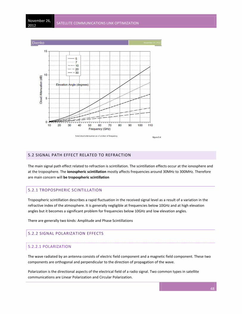
November 26, 2012
SATELLITE COMMUNICATIONS LINK OPTIMIZATION
48
5.2 SIGNAL PATH EFFECT RELATED TO REFRACTION
The main signal path effect related to refraction is scintillation. The scintillation effects occur at the ionosphere and
at the troposphere. The ionospheric scintillation mostly affects frequencies around 30MHz to 300MHz. Therefore
are main concern will be tropospheric scintillation
5.2.1 TROPOSPHERIC SCINTILLATION
Tropospheric scintillation describes a rapid fluctuation in the received signal level as a result of a variation in the
refractive index of the atmosphere. It is generally negligible at frequencies below 10GHz and at high elevation
angles but it becomes a significant problem for frequencies below 10GHz and low elevation angles.
There are generally two kinds: Amplitude and Phase Scintillations
5.2.2 SIGNAL POLARIZATION EFFECTS
5.2.2.1 POLARIZATION
The wave radiated by an antenna consists of electric field component and a magnetic field component. These two
components are orthogonal and perpendicular to the direction of propagation of the wave.
Polarization is the directional aspects of the electrical field of a radio signal. Two common types in satellite
communications are Linear Polarization and Circular Polarization.

[SATELLITE COMMUNICATIONS LINK OPTIMIZATION] November 26, 2012
49
Linear Polarization: The electric field is wholly in one plane containing the direction of propagation. There are two
types; Horizontal and Vertical Polarization.
Horizontal Polarization: The electric field lies in a plane parallel to the earth’s surface
Vertical Polarization: The electric field lies in a plane perpendicular to the earth’s surface.
Circular Polarization: The electric field radiates energy in both the horizontal and vertical planes and all planes in
between.
Right Hand Circular Polarization (RHCP) The electric field is rotating in the clockwise direction as seen by an
observer towards whom the wave is moving
Left Hand Circular Polarization (LHCP) The electric field is rotating in the counterclockwise direction as seen by an
observer towards whom the wave is moving.
5.2.2.2 RAIN DEPOLARIZATION
It refers to the change in the polarization characteristics of a radio wave. A depolarized radio wave will have its
polarization state altered such that power is transferred from the desired polarization state to an undesired
polarization channel.
Rain depolarization can be a problem in the frequency bands above about 12GHz, particularly for frequency reuse
systems communications links the same frequency bands to increase channel capacity.
5.2.2.3 FARADAYS ROTATION
Faraday rotation is an ionospheric effect.
-The ionosphere is a charged layer of the atmosphere.
- When the electromagnetic RF signal passes through the ionosphere, the electric field rotates the polarization
plane of the signal.
- Therefore, the plane of polarization of linearly polarized signals (H / V) twists.
- Faraday rotation has no effect on circular polarization.
- Faraday rotation is dependent on the charged state of the atmosphere, which is dependent on solar activity.

November 26, 2012
SATELLITE COMMUNICATIONS LINK OPTIMIZATION
50
- Sun-spot activity can increase Faraday rotation.
- This polarization rotation causes signal depolarization and increased cross-pol interference.
PART III PART ΙΙΙ
OPTIMIZATION TECHNIQUES AS APPLIED TO
SATELLITE COMMUNICATIONS LINK
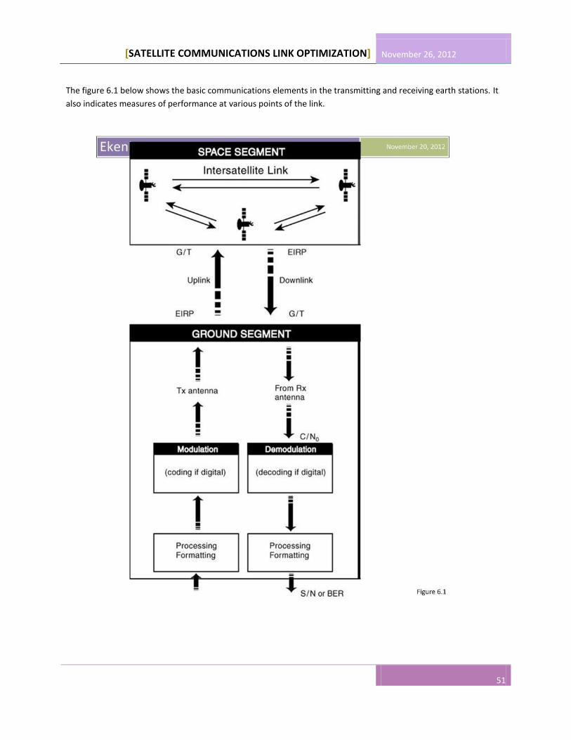
[SATELLITE COMMUNICATIONS LINK OPTIMIZATION] November 26, 2012
51
The figure 6.1 below shows the basic communications elements in the transmitting and receiving earth stations. It
also indicates measures of performance at various points of the link.
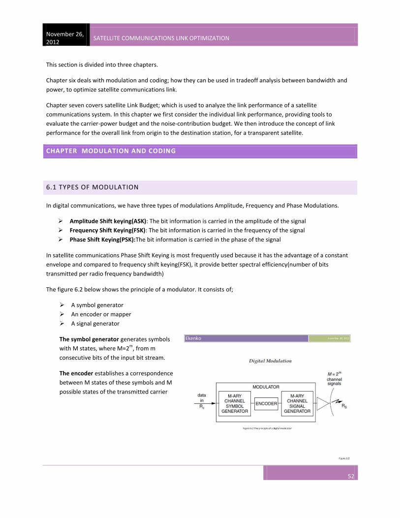
November 26, 2012
SATELLITE COMMUNICATIONS LINK OPTIMIZATION
52
This section is divided into three chapters.
Chapter six deals with modulation and coding; how they can be used in tradeoff analysis between bandwidth and
power, to optimize satellite communications link.
Chapter seven covers satellite Link Budget; which is used to analyze the link performance of a satellite
communications system. In this chapter we first consider the individual link performance, providing tools to
evaluate the carrier-power budget and the noise-contribution budget. We then introduce the concept of link
performance for the overall link from origin to the destination station, for a transparent satellite.
CHAPTER MODULATION AND CODING
6.1 TYPES OF MODULATION
In digital communications, we have three types of modulations Amplitude, Frequency and Phase Modulations.
Amplitude Shift keying(ASK): The bit information is carried in the amplitude of the signal
Frequency Shift Keying(FSK): The bit information is carried in the frequency of the signal
Phase Shift Keying(PSK):The bit information is carried in the phase of the signal
In satellite communications Phase Shift Keying is most frequently used because it has the advantage of a constant
envelope and compared to frequency shift keying(FSK), it provide better spectral efficiency(number of bits
transmitted per radio frequency bandwidth)
The figure 6.2 below shows the principle of a modulator. It consists of;
A symbol generator
An encoder or mapper
A signal generator
The symbol generator generates symbols
with M states, where M=2m
, from m
consecutive bits of the input bit stream.
The encoder establishes a correspondence
between M states of these symbols and M
possible states of the transmitted carrier

[SATELLITE COMMUNICATIONS LINK OPTIMIZATION] November 26, 2012
53
6.1.1 TYPES OF PHASE SHIFT KEYING MODULATION AND BANDWIDTH EFFICIENCY
Depending on the number m, of bits per symbol, different M-ary Phase Shift Keying modulation can be
considered.
Binary Phase Shift Keying (BPSK): If a single bit is used to defined a symbol, a basic two state modulation (M=2) is
defined called BPSK
Quadrature Phase Shift Keying (QPSK): if two consecutive bits are grouped to define a symbol, a four state
modulation (M=4) is defined called QPSK
8-Phase Shift Keying (8PSK): If three consecutive bits are grouped to define a symbol, an eight state modulation
(M=8) is defined called 8-PSK, as shown in figure 6.3 below.
Higher Order Modulation (M=16, 32): This can be obtain for m=4, 5 etc. bits per symbol. As the order of the
modulation increases, the spectral (bandwidth) efficiency increases with increase in the number of bits per symbol.
That is: BPSK uses one bit per symbol
QPSK two bits per symbol- use half the bandwidth
8-PSK three bits per symbol- use one third of the bandwidth
With a modulation of higher order M , better performance is achieved by considering hybrid amplitude and
phase shift keying (APSK), also called Quadrature Amplitude Modulation (QAM). The state of the carrier
corresponds to given values of carrier phase and carrier amplitude (2 for 16APSK, 3 for 32APSK)
16-QAM for example takes four bit per symbol and uses one fourth of the bandwidth.
As we move from 8-PSK to 16-APSK, 32APSK,
the drawback is that the signal is also affected
by the non-linear components like the
amplifiers at the earth station transmitter and
at the satellite.
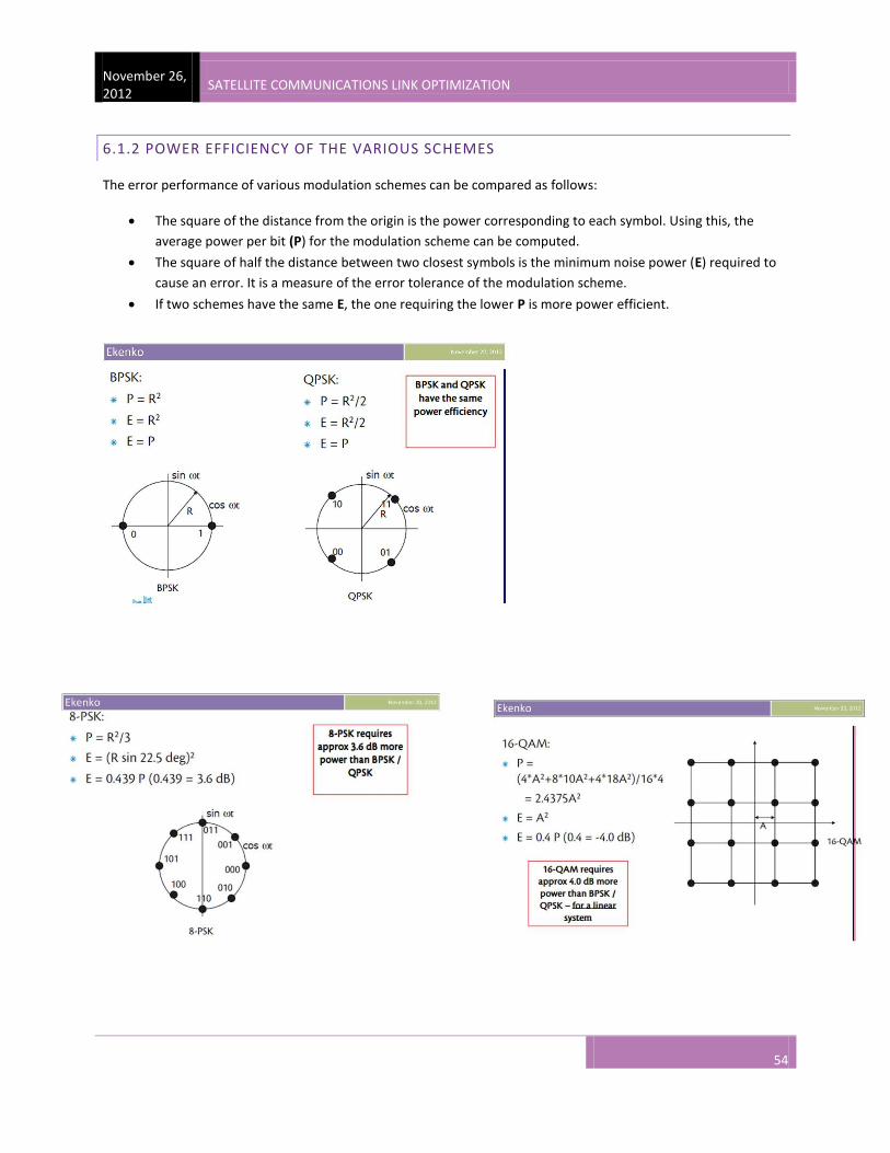
November 26, 2012
SATELLITE COMMUNICATIONS LINK OPTIMIZATION
54
6.1.2 POWER EFFICIENCY OF THE VARIOUS SCHEMES
The error performance of various modulation schemes can be compared as follows:
The square of the distance from the origin is the power corresponding to each symbol. Using this, the
average power per bit (P) for the modulation scheme can be computed.
The square of half the distance between two closest symbols is the minimum noise power (E) required to
cause an error. It is a measure of the error tolerance of the modulation scheme.
If two schemes have the same E, the one requiring the lower P is more power efficient.
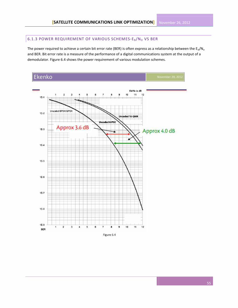
[SATELLITE COMMUNICATIONS LINK OPTIMIZATION] November 26, 2012
55
6.1.3 POWER REQUIREMENT OF VARIOUS SCHEMES-EB/NO VS BER
The power required to achieve a certain bit error rate (BER) is often express as a relationship between the Eb/No
and BER. Bit error rate is a measure of the performance of a digital communications system at the output of a
demodulator. Figure 6.4 shows the power requirement of various modulation schemes.
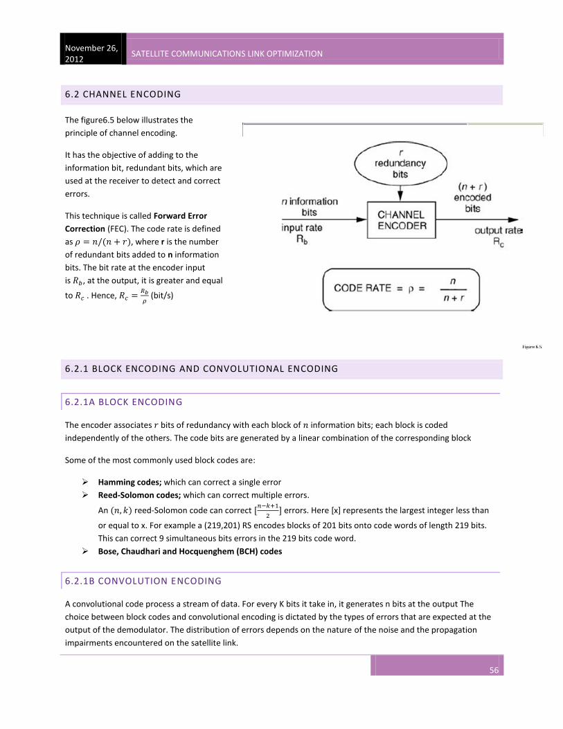
November 26, 2012
SATELLITE COMMUNICATIONS LINK OPTIMIZATION
56
6.2 CHANNEL ENCODING
The figure6.5 below illustrates the
principle of channel encoding.
It has the objective of adding to the
information bit, redundant bits, which are
used at the receiver to detect and correct
errors.
This technique is called Forward Error
Correction (FEC). The code rate is defined
as , where r is the number
of redundant bits added to n information
bits. The bit rate at the encoder input
is , at the output, it is greater and equal
to . Hence,
(bit/s)
6.2.1 BLOCK ENCODING AND CONVOLUTIONAL ENCODING
6.2.1A BLOCK ENCODING
The encoder associates bits of redundancy with each block of information bits; each block is coded
independently of the others. The code bits are generated by a linear combination of the corresponding block
Some of the most commonly used block codes are:
Hamming codes; which can correct a single error
Reed-Solomon codes; which can correct multiple errors.
An reed-Solomon code can correct
errors. Here [x] represents the largest integer less than
or equal to x. For example a (219,201) RS encodes blocks of 201 bits onto code words of length 219 bits.
This can correct 9 simultaneous bits errors in the 219 bits code word.
Bose, Chaudhari and Hocquenghem (BCH) codes
6.2.1B CONVOLUTION ENCODING
A convolutional code process a stream of data. For every K bits it take in, it generates n bits at the output The
choice between block codes and convolutional encoding is dictated by the types of errors that are expected at the
output of the demodulator. The distribution of errors depends on the nature of the noise and the propagation
impairments encountered on the satellite link.

[SATELLITE COMMUNICATIONS LINK OPTIMIZATION] November 26, 2012
57
Under stable propagation conditions and Gaussian noise, errors occur randomly and convolutional encoding is
mostly used. Under fading conditions, errors occur mostly in bursts, compared with convolutional encoding; block
encoding is less sensitive to bursts of errors, so block encoding is preferred.
6.2.2 CONCATENATED ENCODING
The concatenated coding wraps a convolutional code inside a Reed-Solomon code, with an interleaver. The
convolutional code corrects must of the channel errors. When a convolutional code causes errors, the errors are in
bursts. The interleaver spreads the bursts of errors over multiple Reed-Solomon code words. The Reed-Solomon
code then corrects the remaining errors.
Concatenated coding provides very significant improvement in performance over either types of coding alone.
INPUT
OUTPUT
Overall code rate =
*
6.2.3 TURBO CODES
There are a complete replacement for convolutional and Reed-Solomon codes
6.2.4 LOW DENSITY PARITY CHECK CODES (LDPC)
LDPC codes have been found to offer better performance than Turbo codes
LDPC block codes (just like RS block codes) are often used as part of a concatenated coding schemes e.g. the
DVB-S2 standard uses LDPC inner codes and BCH outer codes. This concatenated coding yields better performance.
6.3 CHANNEL DECODING
With FEC, the decoder uses the redundancy introduced at the encoder to detect and correct errors. Various
possibilities are available for decoding block codes and convolutional encoding. Convolutional codes are mostly
RS Encoder Interleaver Convolutional
Encoder
Channel
Convolutional
decoder
De-interleaver RS Decoder
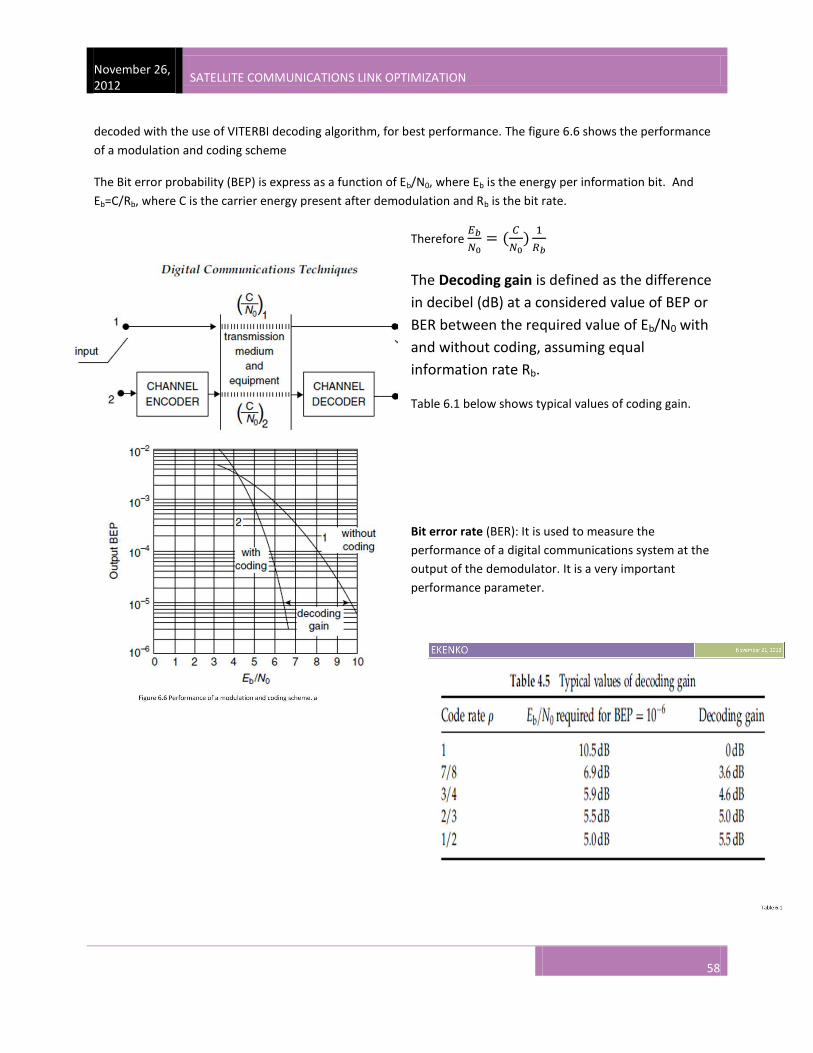
November 26, 2012
SATELLITE COMMUNICATIONS LINK OPTIMIZATION
58
decoded with the use of VITERBI decoding algorithm, for best performance. The figure 6.6 shows the performance
of a modulation and coding scheme
The Bit error probability (BEP) is express as a function of Eb/N0, where Eb is the energy per information bit. And
Eb=C/Rb, where C is the carrier energy present after demodulation and Rb is the bit rate.
Therefore
The Decoding gain is defined as the difference
in decibel (dB) at a considered value of BEP or
BER between the required value of Eb/N0 with
and without coding, assuming equal
information rate Rb.
Table 6.1 below shows typical values of coding gain.
Bit error rate (BER): It is used to measure the
performance of a digital communications system at the
output of the demodulator. It is a very important
performance parameter.
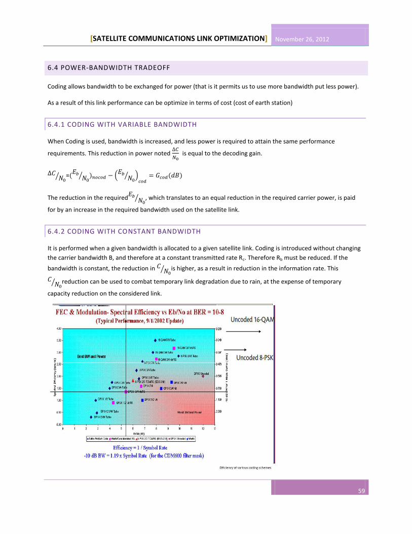
[SATELLITE COMMUNICATIONS LINK OPTIMIZATION] November 26, 2012
59
6.4 POWER-BANDWIDTH TRADEOFF
Coding allows bandwidth to be exchanged for power (that is it permits us to use more bandwidth put less power).
As a result of this link performance can be optimize in terms of cost (cost of earth station)
6.4.1 CODING WITH VARIABLE BANDWIDTH
When Coding is used, bandwidth is increased, and less power is required to attain the same performance
requirements. This reduction in power noted
is equal to the decoding gain.
⁄ =
⁄ (
⁄ )
The reduction in the required
⁄ , which translates to an equal reduction in the required carrier power, is paid
for by an increase in the required bandwidth used on the satellite link.
6.4.2 CODING WITH CONSTANT BANDWIDTH
It is performed when a given bandwidth is allocated to a given satellite link. Coding is introduced without changing
the carrier bandwidth B, and therefore at a constant transmitted rate Rc. Therefore Rb must be reduced. If the
bandwidth is constant, the reduction in ⁄ is higher, as a result in reduction in the information rate. This
⁄ reduction can be used to combat temporary link degradation due to rain, at the expense of temporary
capacity reduction on the considered link.

November 26, 2012
SATELLITE COMMUNICATIONS LINK OPTIMIZATION
60
CHAPTER 7 SATELLITE LINK BUDGET
A satellite link budget is like a financial budget in which:
Signal power = Credit/Income
Noise power = Debit/Expense
A link budget is the basic tool of the satellite engineer. It is used to predict the performance of a satellite link at the
receive terminal by;
Computing the power gain/loses along the satellite link
Computing the impact of various impairments along the satellite link
The main goal of a link budget is to determine;
The Forward link budget : Given the power at the transmit terminal, predict the link performance at the
receive terminal
Reversed Link Budget: Determine the power at the transmit terminal required to achieve a desired link
performance at the receive terminal.
We will begin this section by looking at the configuration of a satellite links. The Links we are talking of here are;
Uplink from a transmit earth station to the satellite
Downlink from a satellite to a receive terminal earth station
End-to-End link from a transmit earth station through the satellite to a receive earth station.
We will then proceed to analyze the performance of each individual link and conclude with that of an overall (end-
to-end) link of a transparent satellite.
7.1 CONFIGURATION OF A LINK
The figure 7.1 represents the elements
participating in a link. The transmit
equipment consist of a transmitter Tx,
connected by a feeder to the transmit
antenna of gain GT in the direction of the
receiver. Power radiated by the transmit
equipment in the direction of the receive
equipment is PT
The performance of the transmit equipment
is measured by its effective isotropic
radiated power (EIRP), defined as
EIRP = (7.1)

[SATELLITE COMMUNICATIONS LINK OPTIMIZATION] November 26, 2012
61
On its way the radiated power suffers from path loss L.
The receiving equipment consists of a receiving antenna of gain GR in the direction of the transmit equipment. The
antenna is connected by a feeder to the receiver Rx. At the receiver input, the power of the modulated carrier is C
and all sources of noise in the link contribute to the system noise temperature T.
The system noise temperature T conditions the noise power spectral density N0, which is used to determine the
performance of the RF link at the input of the receiver ⁄
The performance of the receiving equipment is measured by its figure of merit, ⁄ , where G represents the
overall receiving equipment gain
The following section presents definitions of the relevant parameters that condition the link performance and
provide useful equations that help in calculating ⁄ .
7.2 ANTENNA PARAMETERS
7.2.1 ANTENNA GAINS
The gain of an antenna is the power radiated (or received) per unit solid angle by the antenna in a given direction to
the power radiated (or received) per unit solid angle by an Isotropic antenna fed with the same power. The gain of
the antenna is maximum, in the direction of maximum radiation (boresight) and has a value given by;
( ⁄ )
Where λ ⁄ and is the velocity of light and frequency of the electromagnetic wave. For an
antenna, with a circular aperture, or reflector of diameter D. The surface area
, but ,
where η is the antenna efficiency. Therefore (
)
(
⁄ )
Expressed in dBi (the gain relative to an isotropic antenna), the actual maximum antenna gain is;
(
) ( (
)
)
The efficiency η of the antenna is the product of several factors which take account of the spill-over loss, surface
impairments, ohmic and impedance mismatch losses.
7.2.2 RADIATION PATTERN AND ANGULAR BEAMWIDTH
The radiation pattern indicates the variation of gain with direction. Figure 7.2a and 7.2b show the radiation pattern
for a circular antenna in polar (7.2a) and Cartesian (7.2b) coordinates. The main lobe contains the direction of
maximum radiation. The side lobes should be kept to a minimum.
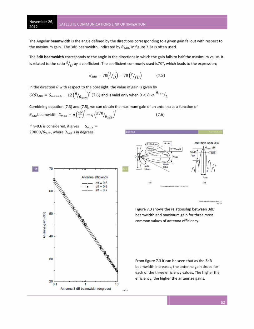
November 26, 2012
SATELLITE COMMUNICATIONS LINK OPTIMIZATION
62
The Angular beamwidth is the angle defined by the directions corresponding to a given gain fallout with respect to
the maximum gain. The 3dB beamwidth, indicated by , in figure 7.2a is often used.
The 3dB beamwidth corresponds to the angle in the directions in which the gain falls to half the maximum value. It
is related to the ratio ⁄ by a coefficient. The coefficient commonly used is , which leads to the expression;
( ⁄ ) ( ⁄ )
In the direction with respect to the boresight, the value of gain is given by
( ⁄ )
and is valid only when
⁄
Combining equation (7.3) and (7.5), we can obtain the maximum gain of an antenna as a function of
beamwidth (
)
(
⁄ )
If η=0.6 is considered, it gives
, where is in degrees.
Figure 7.3 shows the relationship between 3dB
beamwidth and maximum gain for three most
common values of antenna efficiency.
From figure 7.3 it can be seen that as the 3dB
beamwidth increases, the antenna gain drops for
each of the three efficiency values. The higher the
efficiency, the higher the antennae gains.
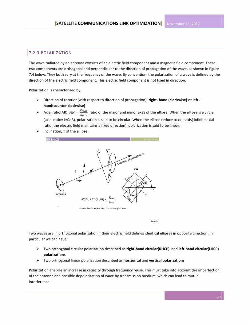
[SATELLITE COMMUNICATIONS LINK OPTIMIZATION] November 26, 2012
63
7.2.3 POLARIZATION
The wave radiated by an antenna consists of an electric field component and a magnetic field component. These
two components are orthogonal and perpendicular to the direction of propagation of the wave, as shown in figure
7.4 below. They both vary at the frequency of the wave. By convention, the polarization of a wave is defined by the
direction of the electric field component. This electric field component is not fixed in direction.
Polarization is characterized by;
Direction of rotation(with respect to direction of propagation); right- hand (clockwise) or left-
hand(counter clockwise)
Axial ratio(AR);
, ratio of the major and minor axes of the ellipse. When the ellipse is a circle
(axial ratio=1=0dB), polarization is said to be circular. When the ellipse reduce to one axis( infinite axial
ratio, the electric field maintains a fixed direction), polarization is said to be linear.
Inclination, of the ellipse
Two waves are in orthogonal polarization if their electric field defines identical ellipses in opposite direction. In
particular we can have;
Two orthogonal circular polarization described as right-hand circular(RHCP) and left-hand circular(LHCP)
polarizations
Two orthogonal linear polarization described as horizontal and vertical polarizations
Polarization enables an increase in capacity through frequency reuse. This must take into account the imperfection
of the antenna and possible depolarization of wave by transmission medium, which can lead to mutual
interference.

November 26, 2012
SATELLITE COMMUNICATIONS LINK OPTIMIZATION
64
Consider figure 7.5 below with two
orthogonal lineally polarized waves.
Amplitude of the wave A, transmitted
with vertical polarization ac
amplitude of wave B, transmitted
with horizontal linear polarization bc
=energy of signal B, found in A due to
depolarization
= energy of signal A, found in B due to
depolarization
The following can be defined
The Cross- Polarization Isolation:
⁄
⁄
(
⁄ ) Or (
⁄ )
The Cross-Polarization Discrimination
⁄ (
⁄ ) (when a single polarization is
transmitted)
7.3 RADIATED POWER
7.3.1 EFFECTIVE ISOTROPIC RADIATED POWER (EIRP)
It is the parameter that characterizes the performance of a transmit equipment and it is given by
To obtain EIRP, we consider the power radiated by an isotropic antenna fed from a radio-frequency source of
power PT, given by
⁄
In a direction where the value of the transmitted gain is , any antenna radiates a power per unit solid angle given
by
, the product is called the EIRP
7.3.2 POWER FLUX DENSITY
A surface area A situated at a distance R from the transmitting antenna, subtends a solid angle A/R2 at the
transmitting antenna as shown in figure 7.6. It receives a power equal to
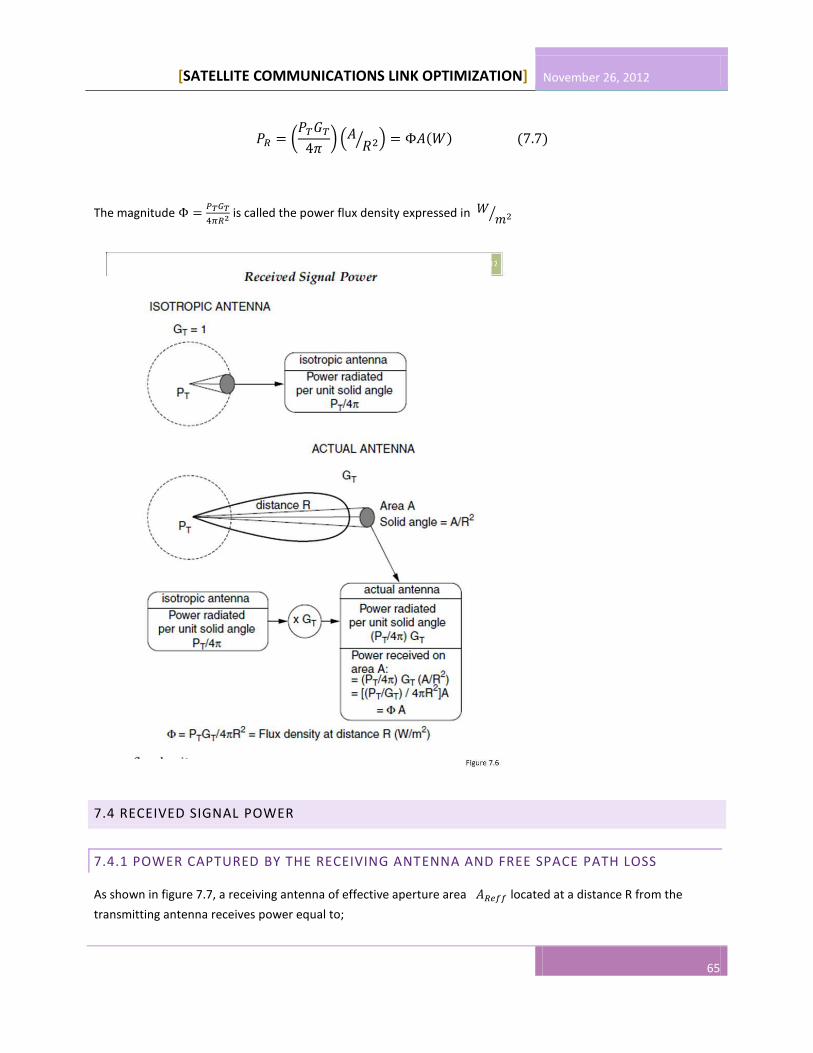
[SATELLITE COMMUNICATIONS LINK OPTIMIZATION] November 26, 2012
65
(
) (
⁄ )
The magnitude
is called the power flux density expressed in ⁄
7.4 RECEIVED SIGNAL POWER
7.4.1 POWER CAPTURED BY THE RECEIVING ANTENNA AND FREE SPACE PATH LOSS
As shown in figure 7.7, a receiving antenna of effective aperture area located at a distance R from the
transmitting antenna receives power equal to;

November 26, 2012
SATELLITE COMMUNICATIONS LINK OPTIMIZATION
66
(
)
The effective area of an antenna is expressed as a function of its receiving gain according to equation (7.2)
(
)
Hence an expression for the received power (
)
(
) ( (
))
(
)
( ⁄ )
Where (
)
is called the free space loss and represents it is usually of the order of 200dB for an earth
station situated at an altitude of about 35786Km. It is loss linked to the distance that exists between the
transmitting equipment and the receiving equipment. It is not linked to any attenuation.
7.5 ADDITIONAL LOSSES
In practice, it is necessary to take into account additional losses due to various causes
Attenuation of the wave as they propagate through the atmosphere
Losses in transmitting and receiving equipment
Depointing losses
Polarization mismatch losses

[SATELLITE COMMUNICATIONS LINK OPTIMIZATION] November 26, 2012
67
7.5.1 ATTENUATION IN THE ATMOSPHERE
The attenuation of waves in the atmosphere, denoted by , is due to the presence of gaseous components in the
troposphere, water (rain, clouds, snow and ice) and ionosphere. The overall effect on the power of the received
carrier can be taken into account by replacing in equation (7.9) by the Path Loss, L, where
7.5.2 LOSSES IN THE TRANSMITTING AND RECEIVING EQUIPMENT
Figure (7.8) shows the losses in the terminal equipment. We have the following;
-The feeder loss between the transmitter and the antenna; to feed the antenna with power PT it is necessary
to provide a power at the output of the transmission amplifier such that;
Expressing the EIRP as a function of the power at the output of the transmission amplifier, we have;
-the feeder loss between the antenna and the receiver; has an impact on the power at the input of the
receiver, , such that it will be equal to
⁄
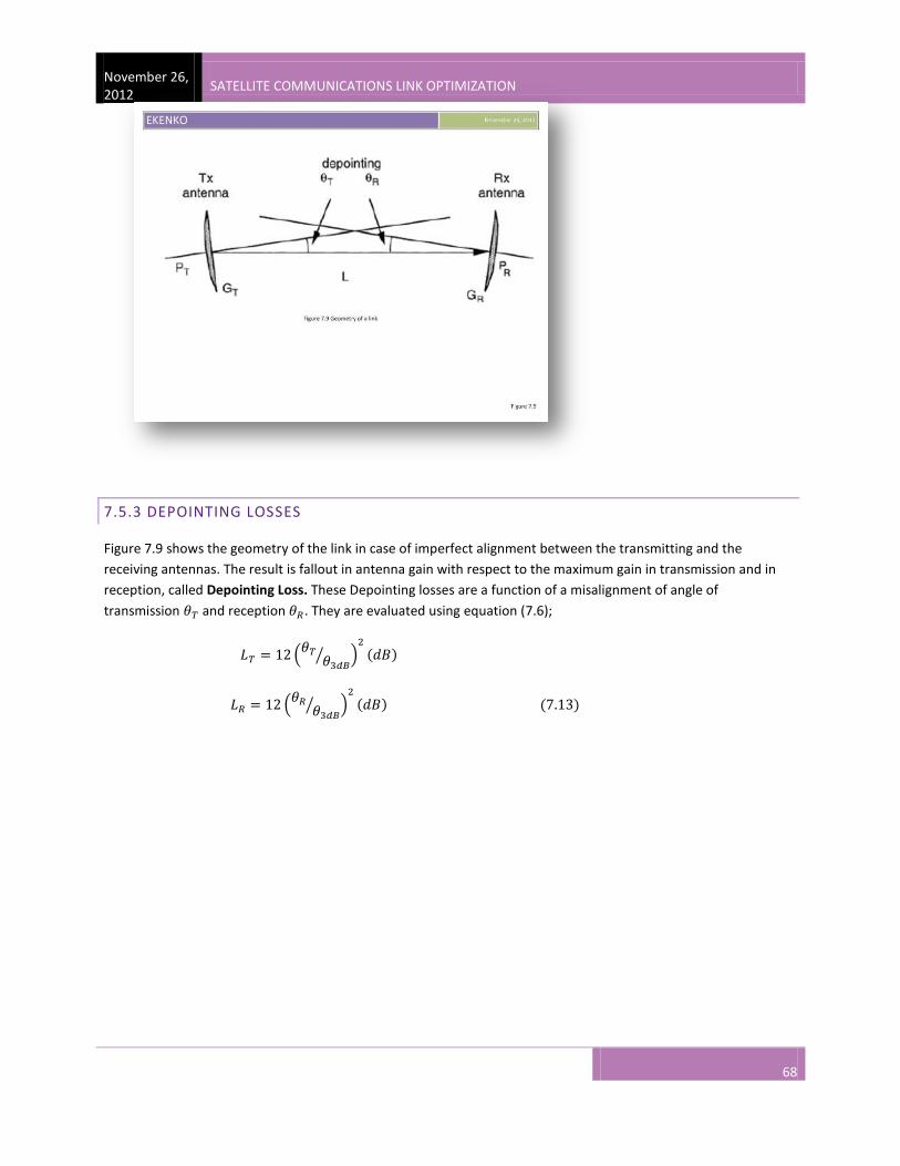
November 26, 2012
SATELLITE COMMUNICATIONS LINK OPTIMIZATION
68
7.5.3 DEPOINTING LOSSES
Figure 7.9 shows the geometry of the link in case of imperfect alignment between the transmitting and the
receiving antennas. The result is fallout in antenna gain with respect to the maximum gain in transmission and in
reception, called Depointing Loss. These Depointing losses are a function of a misalignment of angle of
transmission and reception . They are evaluated using equation (7.6);
(
⁄ )
(
⁄ )
[SATELLITE COMMUNICATIONS LINK OPTIMIZATION] November 26, 2012
69
7.5.4 LOSSES DUE TO POLARIZATION MISMATCH
When the receiving antenna is not oriented with the polarization of the received wave, a polarization mismatch
occurs. In a link with circular polarization the transmitted wave is circularly polarized only on the axis of the
antenna and becomes elliptical off this axis. Propagation through the atmosphere can also change circular into
elliptical polarization.
In linear polarization link, the wave can be subject to rotation of its plane of polarization as it propagates through
the atmosphere. Finally with linear polarization, the receiving antenna may not have its plane of polarization align
with that of the incident wave. If is the angle between the two planes, the polarization mismatch loss
(in dB) is . In a case where a circularly polarized antenna receives a linearly polarized wave,
will have a value of 3dB. Considering all sources of loss, the signal power at the receiver input will be;
(
⁄ ) (
⁄ ) (
⁄ )
7.5.5 CONCLUSION
Equations (7.9) and (7.14), which express the received power at the input to the receiver, are of the same form;
they are a product of three factors;
-EIRP, which characterizes the transmitting equipment
⁄
Which takes into account loss, between the transmit amplifier and the antenna. Reduction in gain LT due to
misalignment of the transmit antenna
-1/L, which characterizes the transmission medium
⁄
⁄
The path loss takes in to account free space attenuation and atmospheric attenuation
-The gain of the receiver, which characterizes the receiving equipment;
⁄
Which takes into account losses, between the antenna and the receiver, LR due to misalignment of receiver
antenna and, ,due to polarization mismatch.

November 26, 2012
SATELLITE COMMUNICATIONS LINK OPTIMIZATION
70
7.6 NOISE POWER SPECTRAL DENSITY AT THE RECEIVER INPUT
7.6.1 ORIGIN OF NOISE
Noise consists of all unwanted contributions whose power adds to the wanted carrier power. It reduces the ability
of the receiver to reproduce correctly the information content of the received wanted carrier.
As seen in chapter 4, noise can originate from;
Thermal source(noise emitted by natural sources of radiation situated around the receiver antenna and
noise generated by components of the receiving equipment)
Interfering sources from neighboring systems
7.6.2 NOISE CHARACTERIZATION
The equivalent noise power captured by a receiver with equivalent noise bandwidth , is given by
Where N0 is the noise power spectral density
7.6.3 NOISE TEMPERATURE OF A NOISE SOURCE
The noise temperature of a noise source of noise power spectral density N0 is given by
⁄
Where k the Boltzmann’s constant = 1.379x10-23
= -228.6dBW/HzK
7.6.4 NOISE FIGURE
If the reference temperature at the input of an element is T0=290K, also if the element has a gain G, a bandwidth B
and is driven by a source of noise temperature T0. The total power at the output is . The noise power
originating from the source is . The noise figure is thus
⁄
The noise figure is usually quoted in decibel (dB): (
⁄ )
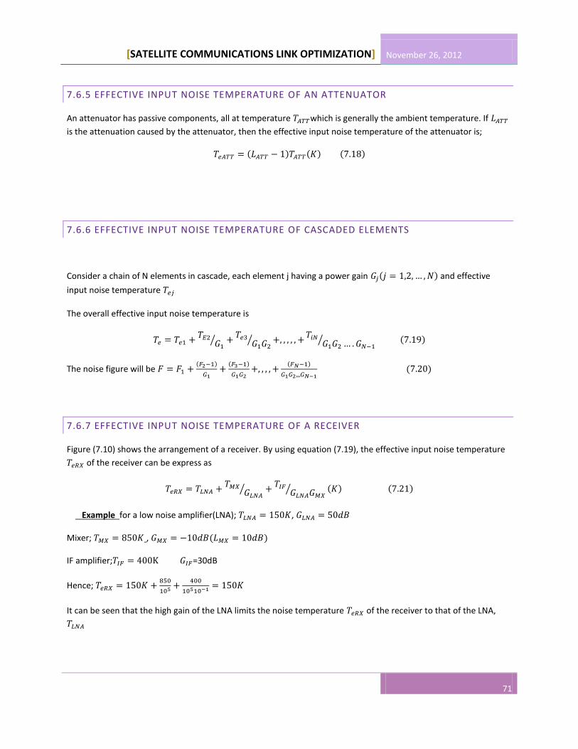
[SATELLITE COMMUNICATIONS LINK OPTIMIZATION] November 26, 2012
71
7.6.5 EFFECTIVE INPUT NOISE TEMPERATURE OF AN ATTENUATOR
An attenuator has passive components, all at temperature which is generally the ambient temperature. If
is the attenuation caused by the attenuator, then the effective input noise temperature of the attenuator is;
7.6.6 EFFECTIVE INPUT NOISE TEMPERATURE OF CASCADED ELEMENTS
Consider a chain of N elements in cascade, each element j having a power gain and effective
input noise temperature
The overall effective input noise temperature is
⁄
⁄
⁄
The noise figure will be
7.6.7 EFFECTIVE INPUT NOISE TEMPERATURE OF A RECEIVER
Figure (7.10) shows the arrangement of a receiver. By using equation (7.19), the effective input noise temperature
of the receiver can be express as
⁄
⁄
Example for a low noise amplifier(LNA); ,
Mixer; ,
IF amplifier; =30dB
Hence;
It can be seen that the high gain of the LNA limits the noise temperature of the receiver to that of the LNA,

November 26, 2012
SATELLITE COMMUNICATIONS LINK OPTIMIZATION
72
7.6.8 ANTENNA NOISE TEMPERATURE
An antenna picks up noise from the radiating bodies within the radiation pattern of the antenna. The noise output
from an antenna is a function of the direction in which the antenna is pointing, it’s radiation pattern and the state
of the surrounding environment
The antenna is assumed to be a noise source characterized by a noise temperature called the noise temperature of
the antenna . Two cases are considered
A satellite antenna (uplink)
An earth station antenna (downlink)
7.6.8 NOISE TEMPERATURE OF A SATELLITE ANTENNA
As seen in chapter 4, noise is captured by this antenna from the earth and from outer space. The earth is the major
contributor. For a beamwidth of 17.5 , the antenna noise temperature depends on the frequency and orbital
position of the satellite. For a smaller beamwidth (spot beam), it depends on the frequency and the area covered.
For a preliminary design, the value 290K can be taken as a conservative value.
7.6.9 NOISE TEMPERATURE OF AN EARTH STATION ANTENNA (DOWNLINK)
It comes from the sky and noise due to radiation from the earth. This is shown in figure (7.11a) and (7.11b), for
clear sky and rain attenuation conditions
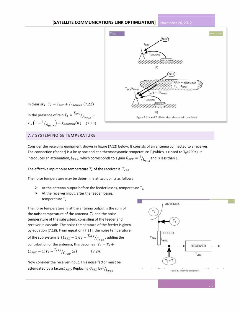
[SATELLITE COMMUNICATIONS LINK OPTIMIZATION] November 26, 2012
73
In clear sky
In the presence of rain
⁄
(
⁄ )
7.7 SYSTEM NOISE TEMPERATURE
Consider the receiving equipment shown in figure (7.12) below. It consists of an antenna connected to a receiver.
The connection (feeder) is a lossy one and at a thermodynamic temperature TF(which is closed to T0=290K). It
introduces an attenuation , which corresponds to a gain
⁄ and is less than 1.
The effective input noise temperature of the receiver is .
The noise temperature may be determine at two points as follows
At the antenna output before the feeder losses, temperature T1;
At the receiver input, after the feeder losses,
temperature T2
The noise temperature T1 at the antenna output is the sum of
the noise temperature of the antenna and the noise
temperature of the subsystem, consisting of the feeder and
receiver in cascade. The noise temperature of the feeder is given
by equation (7.18). From equation (7.21), the noise temperature
of the sub system is
⁄ , adding the
contribution of the antenna, this becomes
⁄
Now consider the receiver input. This noise factor must be
attenuated by a factor . Replacing by ⁄ ,
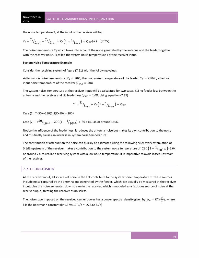
November 26, 2012
SATELLITE COMMUNICATIONS LINK OPTIMIZATION
74
the noise temperature Ts at the input of the receiver will be;
⁄
⁄ (
⁄ )
The noise temperature T2 which takes into account the noise generated by the antenna and the feeder together
with the receiver noise, is called the system noise temperature T at the receiver input.
System Noise Temperature Example
Consider the receiving system of figure (7.21) with the following values.
-Attenuation noise temperature: ; thermodynamic temperature of the feeder; ; effective
input noise temperature of the receiver ;
The system noise temperature at the receiver input will be calculated for two cases: (1) no feeder loss between the
antenna and the receiver and (2) feeder loss . Using equation (7.25)
⁄ (
⁄ )
Case (1): T=50K+290(1-1)K+50K = 100K
Case (2): T= ⁄
⁄ =149.3K or around 150K.
Notice the influence of the feeder loss; it reduces the antenna noise but makes its own contribution to the noise
and this finally causes an increase in system noise temperature.
The contribution of attenuation the noise can quickly be estimated using the following rule: every attenuation of
0.1dB upstream of the receiver makes a contribution to the system noise temperature of ( ⁄ )=6.6K
or around 7K. to realize a receiving system with a low noise temperature, it is imperative to avoid losses upstream
of the receiver.
7.7.1 CONCLUSION
At the receiver input, all sources of noise in the link contribute to the system noise temperature T. These sources
include noise captured by the antenna and generated by the feeder, which can actually be measured at the receiver
input, plus the noise generated downstream in the receiver, which is modeled as a fictitious source of noise at the
receiver input, treating the receiver as noiseless.
The noise superimposed on the received carrier power has a power spectral density given by;
, where
k is the Boltzmann constant (k=1.379x10⁻²
J/K = -228.6dBJ/K)

[SATELLITE COMMUNICATIONS LINK OPTIMIZATION] November 26, 2012
75
7.8 INDIVIDUAL LINK PERFORMANCE
The link performance is evaluated as a ratio of the received carrier power C, to the noise power spectral density, N0
and is quoted as the ⁄ ratio, express in hertz. One can evaluate the link performance using other ratios
besides ⁄ , for instance
⁄ represents the carrier power over the system noise temperature expressed in units of watts
per kelvin (W/K), it is given by ⁄ ⁄ , where k is the Boltzmann constant
⁄ represents carrier power over the noise power; it is dimensionless, it is given by
⁄ ( ⁄ )
⁄ , where is the noise bandwidth
7.8.1 CARRIER TO NOISE POWER SPECTRAL DENSITY RATIO AT THE RECEIVER INPUT
The power received at the receiver input, as given by equation (7.14), is that of the carrier. Hence
The noise power spectral density at the same point is , where T is given by equation (7.25)
Hence
⁄ [(
⁄ ) ( ⁄ ) (
⁄ )] [(
⁄ (
⁄ ) )]
This expression can be interpreted as follows:
⁄
( ⁄ ) (
⁄ ) ( ⁄ )
⁄ Can also be express as a function of the power flux density ;
⁄ (
⁄ ) (
⁄ ) ( ⁄ )
Where
⁄
Finally it can be verified that evaluation of ⁄ is independent of the point chosen in the receiving chain as long as
the carrier power and noise power spectral are calculated at the same point.
Equation (7.27) for C/N0 introduces three factors;
EIRP, which characterizes the transmitting equipment
1/L, which characterizes the transmission medium
The composite receiving gain/noise temperature, which characterizes the receiving equipment; it is called
the figure of merit, or G/T, of the receiving equipment.

November 26, 2012
SATELLITE COMMUNICATIONS LINK OPTIMIZATION
76
By examining equation (7.26), it can be seen that the figure of merit G/T of the receiving equipment is a
function of the antenna noise temperature and the effective input noise temperature of the
receiver. These magnitudes will now be quantified.
In conclusion, equation (7.26) boils down to;
⁄ ( ⁄ )( ⁄ )( ⁄ )
7.8.2 CLEAR SKY CONDITION
Figure (7.13) shows the geometry of the link. It is assumed that the transmitting earth station is on the edge of the
3dB beamwidth coverage of the satellite receiving antenna.
The data used are given below;
-Frequency; =14GHz
For the earth station(ES);
o Transmitting amplifier power;
o Loss between the amplifier and antenna;
o Antenna diameter; D=4m
o Antenna efficiency;
o Maximum pointing error;
Earth station – satellite distance; R= 40,000Km
Atmospheric attenuation; (typical value at this frequency for elevation angle 10 )
For the satellite(SL)
o Receiving beam half power angular width;
o Antenna efficiency;
o Receiver noise figure; F=3dB
o Loss between antenna and receiver;
o Thermodynamic temperature of the connection;
o Antenna noise temperature;
To calculate the EIRP of the earth station;
⁄
[SATELLITE COMMUNICATIONS LINK OPTIMIZATION] November 26, 2012
77
With =100W=20dBW, (
⁄ )
(
⁄ )
( ⁄ )
(
⁄ )
(
⁄ )
,
Hence
To calculate the upward path loss (U);
With (
)
(
)
, Hence
To calculate the figure of merit G/T of the satellite (SL);
( ⁄ )
(
⁄ )
[
⁄ (
⁄ ) ]
With (
)
(
⁄ )
( ⁄ )
(
⁄ )
, Since the earth station is at the edge of the 3dB coverage area,
⁄ ,
Assume , Given
Hence ( ⁄ )
[ ⁄ (
⁄ ) ]
Notice that when the thermodynamic temperature of the feeder between the antenna and the satellite receiver is
close to the antenna noise temperature, which is the case in practice, the uplink system noise temperature at the
receiver input is . It is therefore needlessly costly to install a receiver with a low
noise figure on board the satellite
To calculate the ratio ⁄ for the uplink;
( ⁄ )
(
⁄ ) ( ⁄ )
( ⁄ )
Hence: 71.7dBW – 207.7dB + 6.6dBK-1
+ 228.6dBJ/K =99.2dBHz.
Figure (7.14) shows the path of the signal in uplink and the power at various points
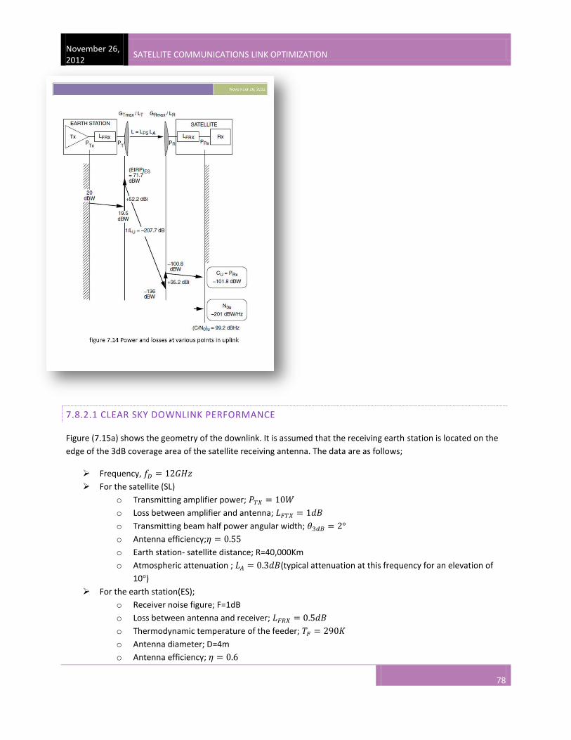
November 26, 2012
SATELLITE COMMUNICATIONS LINK OPTIMIZATION
78
7.8.2.1 CLEAR SKY DOWNLINK PERFORMANCE
Figure (7.15a) shows the geometry of the downlink. It is assumed that the receiving earth station is located on the
edge of the 3dB coverage area of the satellite receiving antenna. The data are as follows;
Frequency,
For the satellite (SL)
o Transmitting amplifier power;
o Loss between amplifier and antenna;
o Transmitting beam half power angular width;
o Antenna efficiency;
o Earth station- satellite distance; R=40,000Km
o Atmospheric attenuation ; (typical attenuation at this frequency for an elevation of
10 )
For the earth station(ES);
o Receiver noise figure; F=1dB
o Loss between antenna and receiver;
o Thermodynamic temperature of the feeder;
o Antenna diameter; D=4m
o Antenna efficiency;

[SATELLITE COMMUNICATIONS LINK OPTIMIZATION] November 26, 2012
79
o Maximum pointing error;
o Ground noise temperature;
To calculate the EIRP of the satellite
⁄
With , (
)
(
⁄ )
( ⁄ )
(
⁄ )
, since the station is at the edge,
⁄ , ,
Hence;
To calculate the downlink path loss (D);
With (
)
(
)
,
Hence;
To calculate the figure of merit G/T of the earth station in the satellite direction;
( ⁄ )
(
⁄ )
is the downlink system noise temperature at the input given by [
⁄ (
⁄ ) ]
And (
)
(
)
(
)
(
⁄ )
(
⁄ )
, ,
, with and , for which
, ,
Hence ⁄ (
⁄ )
( ⁄ )
To calculate the ( ⁄ )
(
⁄ ) ( ⁄ )
( ⁄ )
Hence ( ⁄ )
Figure 7.15b shows the clear sky downlink power variation
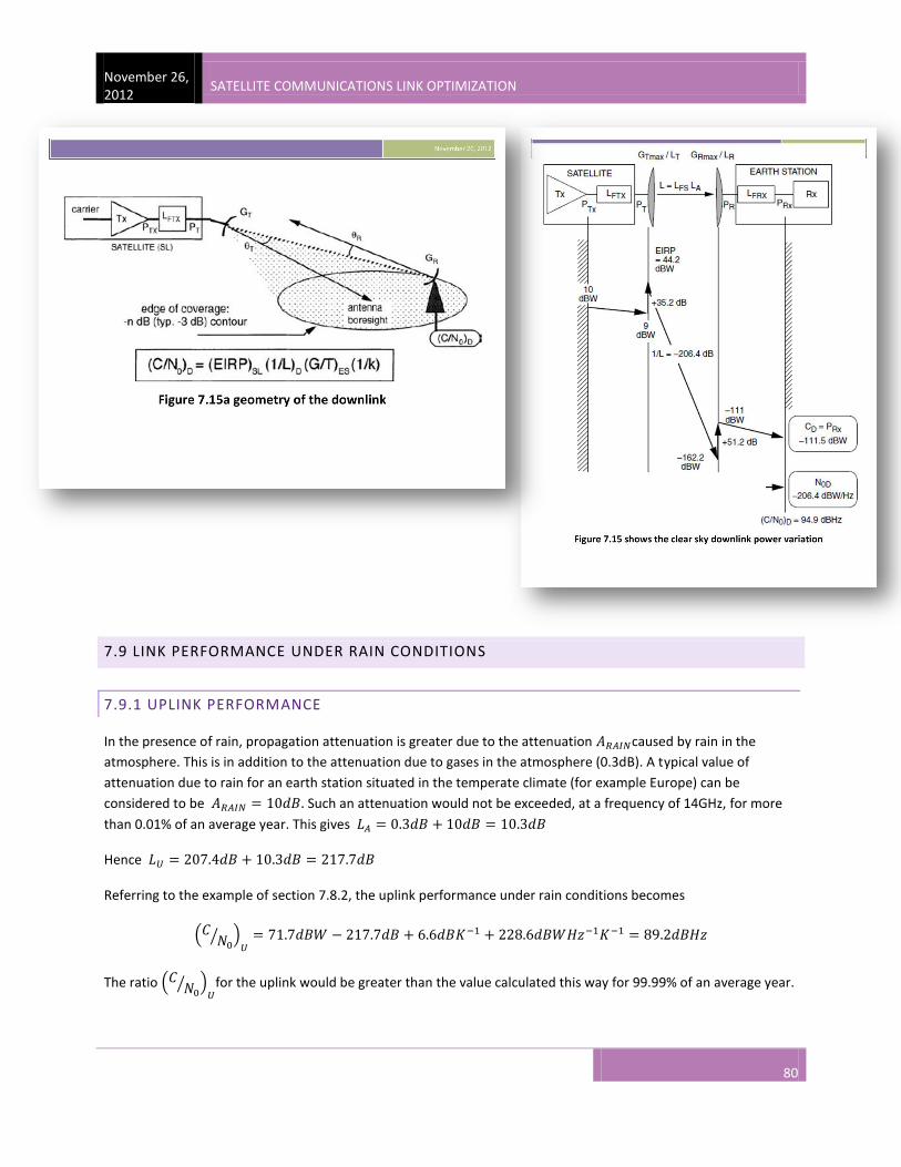
November 26, 2012
SATELLITE COMMUNICATIONS LINK OPTIMIZATION
80
7.9 LINK PERFORMANCE UNDER RAIN CONDITIONS
7.9.1 UPLINK PERFORMANCE
In the presence of rain, propagation attenuation is greater due to the attenuation caused by rain in the
atmosphere. This is in addition to the attenuation due to gases in the atmosphere (0.3dB). A typical value of
attenuation due to rain for an earth station situated in the temperate climate (for example Europe) can be
considered to be Such an attenuation would not be exceeded, at a frequency of 14GHz, for more
than 0.01% of an average year. This gives
Hence
Referring to the example of section 7.8.2, the uplink performance under rain conditions becomes
( ⁄ )
The ratio ( ⁄ )
for the uplink would be greater than the value calculated this way for 99.99% of an average year.
[SATELLITE COMMUNICATIONS LINK OPTIMIZATION] November 26, 2012
81
7.9.2 DOWNLINK PERFORMANCE
Referring now to the example of section 7.8.2.1, is taken as a typical value of the attenuation due to
rain for an earth station in the temperate climate (for example in Europe), which will not be exceeded at a typical
frequency of 12GHz, for more than 0.01% of an average year. This is .
Hence, . The antenna noise temperature is given by
⁄ (
⁄ )
Taking , ⁄ (
⁄ )
⁄ (
⁄ )
Hence( ⁄ )
,
To calculate the ratio ( ⁄ )
(
⁄ ) ( ⁄ )
( ⁄ )
Hence ( ⁄ )
= 84.7dBHz
The ( ⁄ )
ratio for the downlink would be greater than the value calculated in this way for 99.99% of an average
year.
7.9.3 CONCLUSION
The quality of a link between a transmitter and a receiver can be characterized by the ratio of the carrier power to
the noise power spectral density ⁄ . This is a function of the transmitter EIRP, the receiver figure of merit G/T
and the properties of the transmission medium. In a satellite link between two stations, two links must be
considered- the uplink, characterized by the ratio ( ⁄ )
, and the downlink, characterize by the ratio (
⁄ )
.
The propagation conditions in the atmosphere affect the uplink and the downlink differently; rain reduces the value
of the ratio ( ⁄ )
by decreasing the received power , while it reduces the value of(
⁄ )
, by reducing the
value of the received power and increases the downlink system noise temperature. Denoting the resulting
degradation by ( ⁄ ) gives
( ⁄ )
( ⁄ )
( ⁄ )
November 26, 2012
SATELLITE COMMUNICATIONS LINK OPTIMIZATION
82
7.10 OVERALL LINK PERFORMANCE WITH A TRANSPARENT SATELLITE
In this section we will discuss the station-to-station link performance that is a link involving one uplink and one
downlink via a transparent satellite. Up to now the noise on the uplink and downlink has been considered to be
thermal noise only
In practice one has to account for interference noise originating from other carriers in the considered frequency
band and intermodulation noise resulting from multi-carrier operation of non-linear amplifiers.
We will first discuss overall link performance without interference or intermodulation. Then overall link
performance is discussed considering interference and finally intermodulation.
The following notations are used;
( ⁄ )
is the uplink carrier power to noise power spectral density ratio (Hz) at the satellite receiver
input, considering no other noise contributions than the uplink system thermal noise temperature .
( ⁄ )
is the downlink carrier power to noise power spectral density ratio(Hz) at the input of the earth
station receiver, considering no other noise contributions than the downlink system thermal noise
temperature .
( ⁄ )
Carrier power to interference noise power spectral density ratio (Hz) at the input of the
considered receiver.
( ⁄ )
Carrier power to intermodulation noise power spectral density ratio (Hz) at the output of the
considered non-linear amplifier.
( ⁄ )
Overall carrier power to noise power spectral density ratio (Hz) at the earth station receiver
input.
7.10.1 CHARACTERISTICS OF THE SATELLITE CHANNEL
Figure (7.16) shows a transparent payload, the overall bandwidth is split into several sub bands, amplified by a
dedicated power amplifier. The amplifying chain associated with each sub-band is called a satellite channel, or
transponder. The satellite channel amplifies one or several carriers. Here are some notations;
carrier power at the satellite receiver input, at saturation it is denoted
is the power at the input of the satellite channel amplifier (i=input, n=number of carriers)
power at the output of the satellite channel amplifier ( o=output, n=number of carriers)
single carrier operation of a satellite channel amplifier
power at the input to the satellite channel amplifier at saturation in single carrier operation
power at the output of the satellite channel amplifier at saturation in single carrier operation
mode

[SATELLITE COMMUNICATIONS LINK OPTIMIZATION] November 26, 2012
83
Saturation refers to the operation of a satellite channel amplifier to produce maximum output power in
single carrier operation mode. The Operator provides characteristics values of a satellite channel in terms
of flux density at saturation, , and EIRP at saturation, .
7.10.2 SATELLITE POWER FLUX DENSITY AT SATURATION
The power flux density is provided by the transmit station and considered at the satellite receive antenna.
The nominal value of power flux density to drive the satellite channel amplifier at saturation is given by
( ⁄ )
is the front end gain from the input of the satellite receiver to the input of the satellite channel amplifier; is
the loss from the output of the satellite receive antenna to the input of the satellite receiver and is the
satellite receive antenna maximum gain.
The formula assumes that the transmit station is located at the center of the satellite receive coverage.
In practice, the flux density to be provided from a given earth station to drive the satellite channel amplifier to
saturation depends on the location of the transmit earth station within the satellite coverage and the polarization

November 26, 2012
SATELLITE COMMUNICATIONS LINK OPTIMIZATION
84
mismatch of the satellite receiving antenna with respect to the uplink carrier polarization. If the receive satellite
antenna gain in the direction of the transmit earth station experiences a gain fallout , from the maximum gain
and polarization mismatch of , then the actual flux density is
7.10.3 SATELLITE EIRP AT SATURATION
The satellite EIRP at saturation and at boresight, relates to the satellite channel amplifier output power
at saturation, and is given by
Where is the loss from the output of the power amplifier to the transmit antenna and is the transmit
antenna maximum gain
In practice, the , which conditions the available carrier power at a given earth station receiver input is
reduced by the transmit antenna gain fallout , when the earth station is not located at the center of the satellite
transmit antenna coverage.
7.10.4 SATELLITE REPEATER GAIN
The satellite repeater gain, , is the gain from the satellite repeater input to the satellite channel amplifier
output. At saturation it is called
Where the satellite channel amplifier is gain and is the gain from the receiver input to the satellite channel
amplifier input.
7.10.5 INPUT AND OUTPUT BACK-OFF
In practice, the satellite channel amplifier is not always operated at saturation and it is convenient to determine the
operating point Q of the satellite channel amplifier. The point Q is determined by the input power and the
output power . It is also convenient to normalize these quantities with respect to and
respectively. Below are definitions of input back-off and output back-off.
⁄

[SATELLITE COMMUNICATIONS LINK OPTIMIZATION] November 26, 2012
85
⁄
We will leave out the subscript Q for the operating power from now.
7.10.6 CARRIER POWER AT THE SATELLITE RECEIVER INPUT
The carrier power at the satellite receiver input required to drive the satellite channel amplifier to operate at the
considered operating point Q is given by
Expressing carrier in terms of satellite channel amplifier output power, we have
With being the satellite channel amplifier gain at saturation, can be expressed as
Where
, is the carrier power at the satellite receiver input to drive the satellite
channel amplifier at saturation. Can also be expressed as a function of ;
Note that input back-off can also be expressed as a ratio of the power flux density required to operate the
satellite channel amplifier at the considered operation point to the power flux density at saturation
7.10.7 EXPRESSION FOR ( ⁄ )
WITHOUT INTERFERENCE FROM OTHER SYSTEMS OR
INTERMODULATION
The power of the carrier received at the input of the earth station receiver is . The noise at the input of the earth
station receiver correspond to the sum of the following
The downlink system thermal noise considered in isolation ( , given by equation(7.25), which
defines the ratio ⁄ for the downlink (
⁄ )
can be calculated as )
The uplink noise retransmitted by the satellite
Hence ( ⁄ )

November 26, 2012
SATELLITE COMMUNICATIONS LINK OPTIMIZATION
86
Where
⁄ is the total power gain between the satellite receiver input and the earth station
receiver input. G takes into account the satellite repeater gain from the input to the satellite receiver to the
output of the satellite channel amplifier; the gain
⁄ of the satellite transmit antenna including the gain
fallout and the loss from the output of the power amplifier to the transmit antenna; the downlink path loss
and the receiving station composite gain
⁄ . This gives
( ⁄ )
⁄
⁄
⁄
In the above expression, the term represents the carrier power at the satellite receiver input. Hence
⁄ ( ⁄ )
, finally ( ⁄ )
( ⁄ )
( ⁄ )
In this expression;
( ⁄ )
⁄
⁄
⁄ ( ⁄ )
( ⁄ )
(
⁄ ) ( ⁄ )
( ⁄ ) ( ⁄ )
( ⁄ )
and (
⁄ )
are the values of ⁄ for the uplink and downlink when the satellite channel operates
at saturation. represents the downlink attenuation and ( ⁄ )
, the figure of merit of the earth station in the
satellite direction.
7.10.8 EXPRESSION FOR ( ⁄ )
TAKING ACCOUNT OF INTERFERENCE AND
INTERMODULATION
Intermodulation and interference where explained in chapter four. When both effects are taking in to account, we
have
( ⁄ )
( ⁄ )
( ⁄ )
( ⁄ )
( ⁄ )

[SATELLITE COMMUNICATIONS LINK OPTIMIZATION] November 26, 2012
87
CHAPTER 8 OPTIMIZATION
In chapter four we saw the different types of noise that affect a communications link. In chapter five we saw the
atmospheric impairments on a communication link. Chapter 6 presented the different modulation techniques used
to transmit information in satellite communications link and how this techniques together with channel coding help
improve the performance of a satellite communications link. Chapter 7 presented means of evaluation satellite
communications link performance.
This chapter focuses on the various means of optimizing the performance of a fixed satellite link. Some of them can
be applied to mobile satellite link but our focus on fixed end- to-end link.
By optimization we mean providing network with improve reliability and high capacity service. There are basically
two groups of techniques; Power restoral techniques and Signal modification techniques.
Most of these techniques play on the link margin to ensure availability of service.
Before looking at these techniques, let us talk a little on link margin.
8.1 LINK MARGIN
All satellite links are design to function at a certain annual availability. The closer to 100% we demand of our link
availability, the more link margin we need to meet this demand.
Design specifies a value of ⁄ greater or equal to (
⁄ )
during a given percent of time, equal to
(100-p%). For example, 99.99% of time implies p=0.01%. As seen in chapter 7, the attenuation due to rain
causes a reduction of the ratio ⁄ given by
( ⁄ )
(
⁄ )
for uplink and
( ⁄ )
(
⁄ )
( ⁄ ) for the downlink
( ⁄ ) ( ⁄ )
( ⁄ )
Represents a reduction (in dB) of the figure of merit due to increase of noise
temperature
For a successful design (system), one must have a ( ⁄ )
(
⁄ )
This can be achieve by including a margin in the clear sky link budget with defined as
( ⁄ )
(
⁄ )
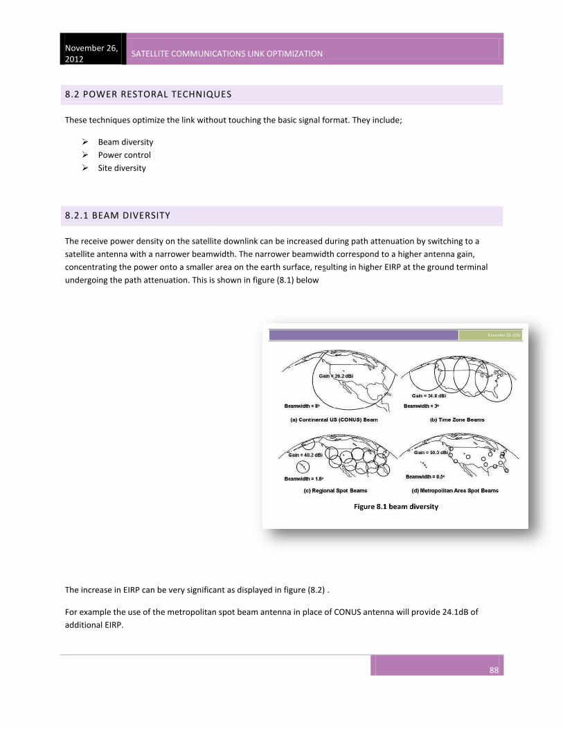
November 26, 2012
SATELLITE COMMUNICATIONS LINK OPTIMIZATION
88
8.2 POWER RESTORAL TECHNIQUES
These techniques optimize the link without touching the basic signal format. They include;
Beam diversity
Power control
Site diversity
8.2.1 BEAM DIVERSITY
The receive power density on the satellite downlink can be increased during path attenuation by switching to a
satellite antenna with a narrower beamwidth. The narrower beamwidth correspond to a higher antenna gain,
concentrating the power onto a smaller area on the earth surface, resulting in higher EIRP at the ground terminal
undergoing the path attenuation. This is shown in figure (8.1) below
The increase in EIRP can be very significant as displayed in figure (8.2) .
For example the use of the metropolitan spot beam antenna in place of CONUS antenna will provide 24.1dB of
additional EIRP.
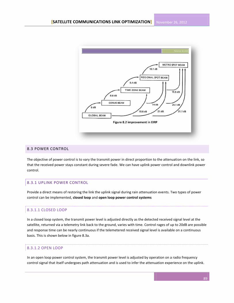
[SATELLITE COMMUNICATIONS LINK OPTIMIZATION] November 26, 2012
89
8.3 POWER CONTROL
The objective of power control is to vary the transmit power in direct proportion to the attenuation on the link, so
that the received power stays constant during severe fade. We can have uplink power control and downlink power
control.
8.3.1 UPLINK POWER CONTROL
Provide a direct means of restoring the link the uplink signal during rain attenuation events. Two types of power
control can be implemented, closed loop and open loop power control systems
8.3.1.1 CLOSED LOOP
In a closed loop system, the transmit power level is adjusted directly as the detected received signal level at the
satellite, returned via a telemetry link back to the ground, varies with time. Control rages of up to 20dB are possible
and response time can be nearly continuous if the telemetered received signal level is available on a continuous
basis. This is shown below in figure 8.3a.
8.3.1.2 OPEN LOOP
In an open loop power control system, the transmit power level is adjusted by operation on a radio frequency
control signal that itself undergoes path attenuation and is used to infer the attenuation experience on the uplink.

November 26, 2012
SATELLITE COMMUNICATIONS LINK OPTIMIZATION
90
This control signal is called Beacon and is sometimes at the same frequency as the uplink. The system is shown in
figure 8.3b
8.4 SITE DIVERSITY
It describes the use of geographically separate ground terminals in a space
communication link to overcome the effect of downlink path attenuation during
intense rain period. It improves overall link performance by taking advantage of
the limited size and extent of intense rain cells. This is shown in figure (8.4)
[SATELLITE COMMUNICATIONS LINK OPTIMIZATION] November 26, 2012
91
8.5 SIGNAL MODIFICATION TECHNIQUES
This involves optimization techniques in which the basic format of the signal is modified.
Space segment costs are typically the most significant operating expense for any satellite-based service, having
direct impact on the viability and profitability of the service. A satellite transponder having finite resources in terms
of bandwidth and power, the transponder leasing costs are determined by bandwidth and power used. For optimal
utilization, a satellite circuit should be design to use similar share of transponder bandwidth and transponder
power.
The traditional approach to balancing a satellite circuit involves trade-off between modulation and coding. A lower
order modulation requires less transponder power at the expense of more bandwidth. Conversely a higher order
modulation reduces required bandwidth, but at a significant increase in power.
Some of the new dimension optimization techniques of satellite communications are; DoubleTalk carrier-in-carrier
(CnC), Adaptive Coding and Modulation (ACM)
8.5.1 OPTIMIZATION BY DOUBLETALK CARRIER-IN-CARRIER
This innovative technology provides a significant improvement in bandwidth and power utilization, beyond what is
possible with traditional with forward error correction (FEC) and modulation alone, allowing users to achieve
unprecedented savings. When combined with advanced modulation and FEC, it allows for multi-dimensional
optimization
o Reducing Operational Expenses(OPEX)
Occupied bandwidth and transponder power
o Reducing Capital Expenditure (CAPEX)
BUC/HPA/ size and antenna size
o Increasing throughput without using additional transponder resources
o Increasing link availability (margin) without using additional transponder resources
o Or a combination to meet different objectives
DoubleTalk Carrier-in-carrier bandwidth compression is based on patented “Adaptive Cancellation” technology that
allows the transmit and receive carriers of a duplex link to share the same transponder space. Figure 8.5a shows
the typical full duplex satellite link, where the two carriers are adjacent to each other. Figure 8.5b shows the
DoubleTalk carrier-in-carrier where the two carriers are overlapping, thus sharing the same spectrum.

November 26, 2012
SATELLITE COMMUNICATIONS LINK OPTIMIZATION
92
DoubleTalk carrier-in-carrier is complementary to all advancement in technology, including advanced FEC and
modulation techniques. As these technologies approach theoretical limits of power and bandwidth efficiencies,
DoubleTalk carrier- in-carrier utilizing advanced signal processing techniques provides a new dimension in
bandwidth and power efficiency.
DoubleTalk carrier-in-carrier allow users to achieve spectral efficiency (bps/Hz) that cannot be achieved with
modulation and FEC alone, example when used with 16-QAM, it approaches the bandwidth efficiency of 256-QAM
(8bps/Hz).
As DoubleTalk carrier-in-carrier allows equivalent spectral efficiency using a lower order modulation and/or FEC
code, it can simultaneously reduce CAPEX by allowing the use of a smaller BUC/HPA and/or antenna
As DoubleTalk carrier-in-
carrier can be used to save
transponder bandwidth
and/or transponder power, it
has been successfully
deployed in bandwidth-
limited as well as power-
limited scenarios.
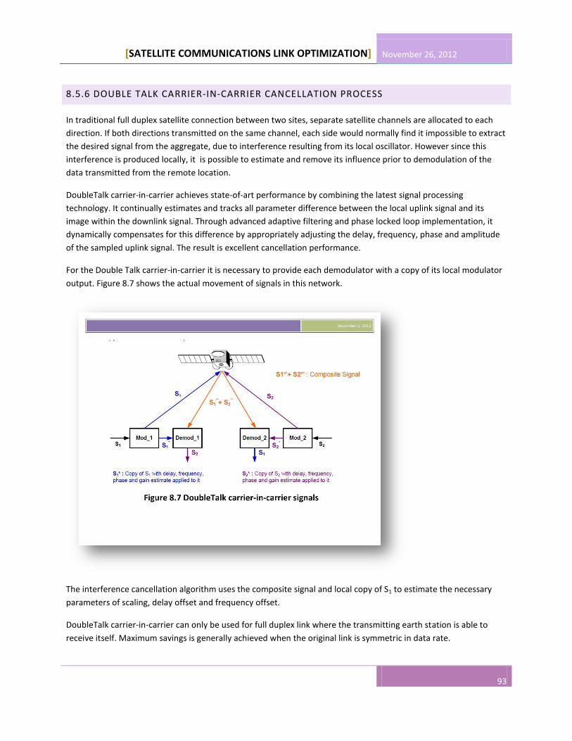
[SATELLITE COMMUNICATIONS LINK OPTIMIZATION] November 26, 2012
93
8.5.6 DOUBLE TALK CARRIER-IN-CARRIER CANCELLATION PROCESS
In traditional full duplex satellite connection between two sites, separate satellite channels are allocated to each
direction. If both directions transmitted on the same channel, each side would normally find it impossible to extract
the desired signal from the aggregate, due to interference resulting from its local oscillator. However since this
interference is produced locally, it is possible to estimate and remove its influence prior to demodulation of the
data transmitted from the remote location.
DoubleTalk carrier-in-carrier achieves state-of-art performance by combining the latest signal processing
technology. It continually estimates and tracks all parameter difference between the local uplink signal and its
image within the downlink signal. Through advanced adaptive filtering and phase locked loop implementation, it
dynamically compensates for this difference by appropriately adjusting the delay, frequency, phase and amplitude
of the sampled uplink signal. The result is excellent cancellation performance.
For the Double Talk carrier-in-carrier it is necessary to provide each demodulator with a copy of its local modulator
output. Figure 8.7 shows the actual movement of signals in this network.
The interference cancellation algorithm uses the composite signal and local copy of S1 to estimate the necessary
parameters of scaling, delay offset and frequency offset.
DoubleTalk carrier-in-carrier can only be used for full duplex link where the transmitting earth station is able to
receive itself. Maximum savings is generally achieved when the original link is symmetric in data rate.

November 26, 2012
SATELLITE COMMUNICATIONS LINK OPTIMIZATION
94
8.6 ADAPTIVE CODING AND MODULATION (ACM)
Adaptive coding and modulation is a statistical, non-static advantage that enables dynamic changes in user
throughput. Benefit and value vary over time and are not guaranteed, but are predictable.
ACM turns fade margin into increased link capacity- gains of 100% or more are possible, compared to
traditional constant coding and modulation (CCM). This is accomplished by automatically adapting the
modulation type and FEC code rate to give highest possible throughput.
ACM maximizes throughput regardless of Link conditions (noise or other impairments, clear sky, rain fade,
etc.). Initial setup is easy, and then requires no further human intervention.
With a CCM system, severe rain fading can cause the total loss of the link, and zero throughput. ACM
keeps the Link up(with lower throughput)-and can yield much higher system availability
It is currently used for IP traffic only.
All satellite links are design to function at a certain annual availability. The closer to 100% we demand of our link
availability, the more link margin we need to meet this demand. Figure 8.8a below is a graph of availability vs. link
margin of a Ku-Band link from Germany to Nigeria. A change in guaranteed annual availability from 99.8% to 99.6%
(as little as 0.2% per year) equates to 17.5 hours per year(365Days*24Hours/day*0.02=17.5Hours).
In this link, it can be seen that this 17.5hours/year demands or saves 2.5dB of link margin. This means that
someone who requires 99.8% availability instead of 99.6% would need an additional 2.5dB link margin for the
entire year. Conversely, deciding to run this link with 99.6% would save 2.5dB of link margin for the entire year.

[SATELLITE COMMUNICATIONS LINK OPTIMIZATION] November 26, 2012
95
Different links have different link margin requirements. Consider the C-Band link between Italy and China with
different link availability characteristics. From figure 8.8b you can clearly see that the same change from 99.6%
availability to 99.8% availability requires a mere 0.35dB of additional link margin.
Because ACM converts link margin into additional user throughput, it can be clearly seen that the greater the link
margin, the greater the benefit of ACM. As link margin is reduced, so too is ACM. I t can also be stated that as
guaranteed availability is increased, link margin will also need to be increased. Conversely as the guaranteed
availability is reduced, link margin will also need to be reduced and the value of ACM will therefore be reduced.
8.6.1 ACM BACKGROUND
The primary function of ACM is to optimize throughput in a wireless data link, by adapting the modulation order
used and the forward error correction(FEC) code rate(which both directly affects spectral efficiency), according to
the noise conditions (or other impairments) on the link.
The implicit in this concept is that the symbol rate (and power) of the wireless communication system must remain
constant. This ensures that the bandwidth allocated for a particular link is never exceeded. Given that the symbol
rate does not change, if modulation and coding are changed, the data rate must therefore be modified.
This is expressed in the simple equation: symbol rate = bit rate/(modulation order*code rate)

November 26, 2012
SATELLITE COMMUNICATIONS LINK OPTIMIZATION
96
Rearranging we have; bit rate = symbol rate*modulation order*code rate
Therefore in changing to a higher order modulation or code rate, the bit rate is increased, and in changing to a
lower order modulation or code rate, the bit rate is reduced.
8.6.2 REQUIREMENTS FOR ACM
a. A modulator and FEC encoder that can instantaneously, when commanded, change either modulation type
(order) or FEC encoder rate, or both. This need to be accomplished without the corruption of data
anywhere in the path. Block FEC codes are considered to be the most practical in achieving the required
synchronization. Recently, a specific nomenclature has emerged to describe a combination of modulation
type and code rate-namely, ModCod. The modulator is required to send the value of the ModCod at the
start of each code block to signal to the demodulator/decoder how to configure the correct modulation
type and FEC code rate.
b. A receiver that is capable of demodulating and decoding the signal transmitted by a) without any prior
knowledge of when a change has taken place, but based purely on the value of the ModCod seen at the
start of each FEC block. Again this need to be accomplished without the corruption of data anywhere in
the path.
c. The receiver in b) need to derive an estimation of the link quality (in terms of
⁄ , , etc.) and then
communicates this estimate, via a return channel, to the modulator in a)
d. The modulator in a) need to be able to process the link metric form the demodulator in b), and then,
based upon a predetermined algorithm, adapt the data rate and change the ModCod sent to the receiver
at the distant end. Thus,
the data rate on the link
can be maximized, given
the current link noise
conditions
A generic example of ACM
over satellite is shown in
figure 8.9a and 8.9b below.
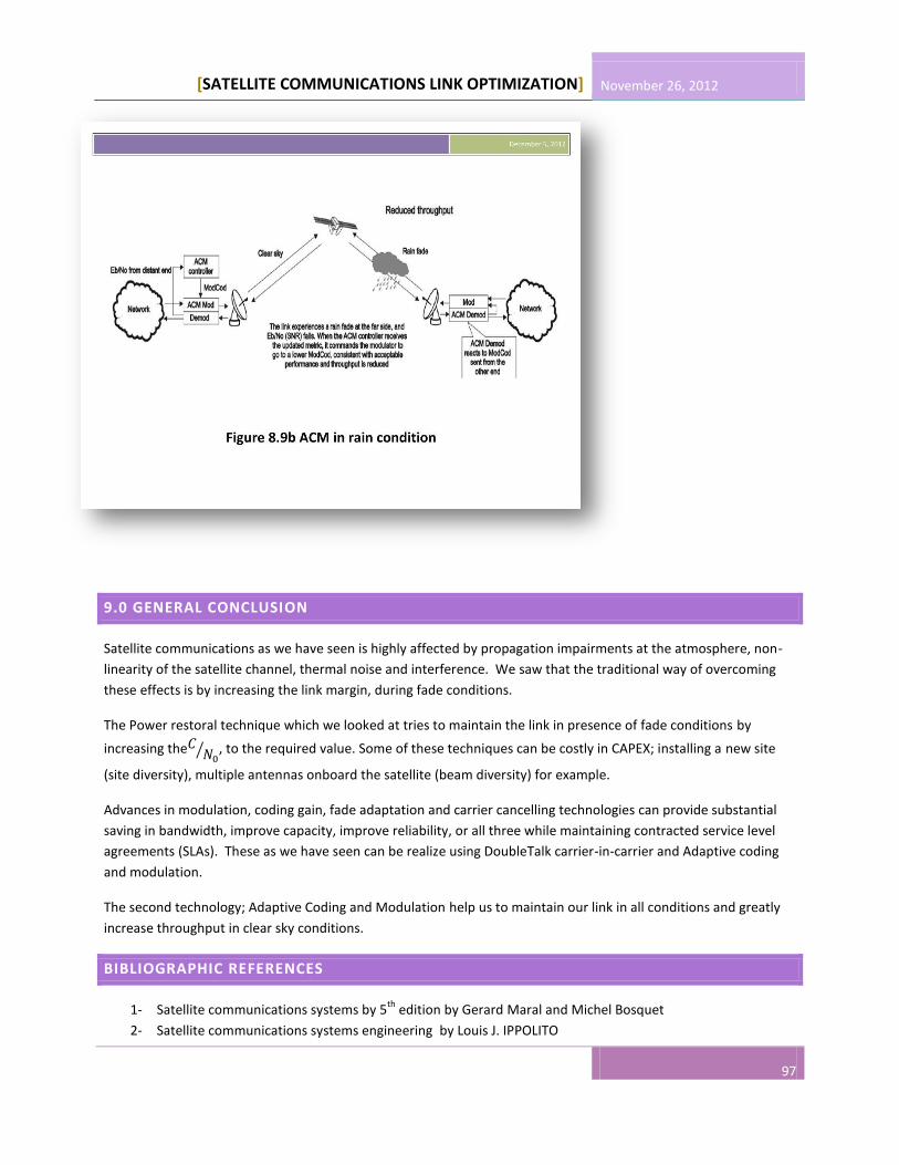
[SATELLITE COMMUNICATIONS LINK OPTIMIZATION] November 26, 2012
97
9.0 GENERAL CONCLUSION
Satellite communications as we have seen is highly affected by propagation impairments at the atmosphere, non-
linearity of the satellite channel, thermal noise and interference. We saw that the traditional way of overcoming
these effects is by increasing the link margin, during fade conditions.
The Power restoral technique which we looked at tries to maintain the link in presence of fade conditions by
increasing the
⁄ , to the required value. Some of these techniques can be costly in CAPEX; installing a new site
(site diversity), multiple antennas onboard the satellite (beam diversity) for example.
Advances in modulation, coding gain, fade adaptation and carrier cancelling technologies can provide substantial
saving in bandwidth, improve capacity, improve reliability, or all three while maintaining contracted service level
agreements (SLAs). These as we have seen can be realize using DoubleTalk carrier-in-carrier and Adaptive coding
and modulation.
The second technology; Adaptive Coding and Modulation help us to maintain our link in all conditions and greatly
increase throughput in clear sky conditions.
BIBLIOGRAPHIC REFERENCES
1- Satellite communications systems by 5th
edition by Gerard Maral and Michel Bosquet
2- Satellite communications systems engineering by Louis J. IPPOLITO


