
September 9, 2008
‘Preliminary version of a paper prepared for the 48th Panel Meeting of Economic Policy in Paris’
Do not quote or cite without authors' permission
Scalpel, Please! Dissecting the Euro’s Effect on Trade*
Volker Nitsch Mauro Pisu ETH Zurich National Bank of Belgium, OECD Abstract In order to identify the effect of the euro on trade, we analyze the pattern and dynamics of cross-border trade between the 15 member countries of the European Union from 1995 to 2005. We apply various statistical techniques to examine trade at various levels of disaggregation, including firm-level trade data for Belgium. We find consistent evidence that trade among member countries of the European Monetary Union (EMU) has moderately increased after the introduction of the euro. However, other important features of a bilateral trade relationship such as the number of traded varieties have remained largely unaffected. At the firm level, we find that the euro has increased the propensity of firms to export to EMU. Also, the number of products that exporters ship to EMU member countries has increased after the introduction of the euro. These effects are stronger for small and less productive firms. In combination with results from aggregate product level, our findings suggest that intra-EMU trade has mainly expanded through the extensive margins, i.e. an increase in the number of exporters and products exported by firms. JEL Code: F13; F14; F15; F33 Keywords: monetary union; common currency; integration * For comments, we thank: Richard Baldwin, Helge Berger, Harry Flam, Franc Klaassen, Philippe Martin, Larry Schembri, anonymous referees, and seminar participants in Amsterdam, Berlin, Duisburg, Ottawa and Zurich. Nitsch thanks Richard Baldwin for encouragement, inspiration and support. Address (corresponding author): Volker Nitsch KOF Swiss Economic Institute Weinbergstrasse 35 8092 Zurich Switzerland Tel.: (044) 632-2553 Fax: (044) 632-1218 E-mail: [email protected]
1. Introduction
1.1 Background
On January 1, 1999, eleven of the (then) fifteen member countries of the European
Union (EU) proceeded in economic integration and formed a monetary union. While
national currencies remained legal tender in the respective countries for the next three
years, their exchange rates were irrevocably fixed to a new multinational currency unit, the
euro, so that any volatility between bilateral nominal exchange rates was completely and
permanently eliminated. After Greece had joined the European Economic and Monetary
Union (EMU) as the twelfth member country on January 1, 2001, the euro was finally
introduced as a physical currency (replacing national notes and coins) on January 1, 2002.1
Although in principle just another step towards integration, the change in the
exchange rate and monetary regime among European countries has attracted much
attention from both policymakers and economists. The effects of EMU are of particular
interest for at least three reasons. First, there have been only very few experiences of
international currency unions before. For instance, in early 1992, when the Maastricht
treaty about the establishment of a monetary union was signed, only 32 of the 166
members of the United Nations (UN) were (periphery) member of a currency union, i.e.,
were not using their own national currency. More importantly, most of the countries
involved in a currency union were radically different from a typical non-currency union
member. Some currency union members were extremely small in size (such as Palau and
Liechtenstein) so that hardly any economic data for these territories were available.2 Other
territories were economically highly dependent on an anchor country (such as Bhutan on
India or Namibia on South Africa), and simply have unilaterally adopted this country’s
currency. Further, almost all pairs of countries in a currency union also shared a common
colonial history (such as the former French colonies that formed the CFA franc zone). In
any case, none of the existing currency unions was comparable with the EMU.
Second, currency unions have been out of fashion for more than 50 years. Since the
end of World War II, not a single currency union had been newly created, and only two
1 On January 1, 2007, Slovenia became the thirteenth member country of EMU. Cyprus and Malta joined EMU one year later. Slovakia is expected to become the sixteenth member country of EMU effective January 1, 2009. 2 Only two of the 17 smallest UN member countries (with a population of less than 150,000) have a sovereign currency (Seychelles, Tonga). More generally, Rose and Engel (2002, Table 1) report a mean population size of about 1.8 million for currency union members, more than an order of magnitude smaller than the average population of 23.6 million in non-currency union member countries.
1

sovereign nations were willing to abandon their independent monies by entering an
existing union: Mali and Guinea-Bissau joined the CFA franc zone in 1984. In contrast,
many territories rather had a strong preference to have their own national currency.
Political separation (e.g., from a former colonizer) was often accompanied by monetary
separation so that the number of currencies in the world has sizably increased in the post-
war period. As a result, Glick and Rose (2002) find that of the 146 regime transitions into
and out of currency unions over the period from 1948 through 1997, 130 switches (~89
percent) in their sample are currency union exits.
Third, recent academic research has argued that the benefits of a common currency
may be substantially larger than initially thought. Rose (2000) finds, in an excellent but
heavily disputed paper, that a common currency is typically associated with much higher
bilateral trade than if two countries use separate currencies; Frankel and Rose (2002)
argue, based on these findings, that membership in a currency union may have a sizable
positive effect on per capita income. Since it seems generally difficult to establish a robust
(negative) empirical relationship between exchange rate volatility and trade (see, for
instance, Clark et al. [2004] for a recent survey of the literature and Tenreyro [2007] for
recent evidence), this finding was highly surprising and controversial.3
Given these uncertainties about the workings of a currency union, the formation of
EMU was widely considered to provide a useful “natural experiment” to identify the
effects of a common currency. The introduction of a new currency among various large,
developed and politically independent nations by free and unforced decision should
provide a perfect environment to extract and analyze the effects of this policy change by
observing possible changes in economic variables after the adoption of the euro. Not
surprisingly, in view of Rose’s (2000) results that sharing the same currency may strongly
benefit trade, a special focus was given on the effects of EMU on trade.
1.2 The euro and trade
A rough exploration of the pattern and dynamics of European trade provides little
conclusive evidence that the introduction of the euro has measurably affected trade.
Table 1 shows for each of the 15 EU member countries that were facing the decision on
whether or not joining EMU in 1999 some illustrative statistics on the (relative)
importance of trade with the EMU; results for the late entrant Greece and for non-EMU 3 In initial calculations of the effects of EMU such as the European Commission’s (1991) study “One Market, One Money”, the trade effects of the euro were expected to be small, especially since exchange rate fluctuations among European currencies were already (very) low.
2

members are presented in bold.4 The first column reports exports to EMU member
countries as a share of a country’s total exports to the EU in 1999, i.e., at a time when the
EMU was established. As the table indicates, there is no measurable difference in the
importance of trade with EMU member countries between EMU and non-EMU countries.
Although there is considerable variation in the geographical structure of exports across
countries, countries outside the EMU do not trade significantly less with EMU member
countries than countries that have decided to participate in the EMU. Also, growth rates of
exports to EMU, shown in the next column, do not differ systematically after the
introduction of the euro5; a similar observation is made for the immediate pre-euro period.
Finally, to identify a possible redirection in EU trade, Figure 1 plots the evolution of the
share of exports to EMU in total exports, scaled to be 1 in 1999. Again, there is no
evidence that the introduction of the euro has measurably changed the pattern of European
trade. Most notably, for countries outside the euro the relative importance of exports to the
EMU is basically unchanged over the sample period; non-EMU countries are at the center
of this fan chart.6
Early regression results that control for the effect of other influences on trade, in
contrast, appear to provide strong support for Rose’s (2000) claim that common currencies
benefit trade. Similar to Rose, these studies apply variants of the widely-used gravity
model of trade to isolate the effect of the euro on trade—a model that allows to hold
constant for a variety of factors, including pre-EMU trade intensity. Studies of this type
typically find that intra-EMU trade has increased by about 10 percent in the first three to
four years of the EMU’s existence. Examples include Micco, Stein and Ordoñez (2003)
and Flam and Nordström (2003); the literature is carefully reviewed in Baldwin (2006a,
2006b). Although the estimated trade effect of the euro is considerably smaller in
magnitude than Rose’s initial estimates suggest, an immediate, economically and
statistically significant increase in trade generally confirms Rose’s main finding, especially
4 In the following, EMU is defined – in time-variant fashion – to comprise all member countries of EMU at a given point in time; the term “euro zone (EZ)” is used as a synonym for this group of countries. Since all of our data covers the period only until 2005, EMU refers to the eleven founding members of EMU plus Greece (EMU12). Occasionally, we also present evidence for the founding members only (EMU11). 5 For almost all countries in the sample exports to EMU have increased by about 20 to 50 percent over the five-year period from 1999 to 2004. However, there are three outliers. Luxembourg’s exports have more than doubled, while exports from the United Kingdom and Greece have increased only by about 10 percent. 6 In similar fashion, Lane (2006, Tables 4 and 5) shows that while international trade as a ratio of GDP has strongly increased for EMU member countries over the last decade, the relative share of trade within the euro area has declined for most member countries.
3

since Glick and Rose (2002) have shown that it may take decades before the trade effect of
a common currency fully shows up.
Results derived from the gravity approach, however, are not without criticisms. In
an early critique of Rose (2000), Persson (2001) applies a non-parametric matching
technique to identify the currency union effect on trade and gets much smaller (though still
significantly positive) estimates. Baldwin (2006a, 2006b) emphasizes that most
applications of the gravity model lack proper theoretical foundation and are seriously
misspecified; this misspecification would lead to considerable overestimation of the
common currency effect on trade. Berger and Nitsch (2008) take a historical perspective
and argue that the increase in trade between EMU member countries that is observed after
the introduction of the euro is simply a continuation of a long-run trend; they show that the
intensity of trade between countries that have later adopted the euro has continuously risen
since the end of World War II.
Apart from methodological issues (producing contradictory results), there are other
sorts of difficulties in identifying the euro’s effect on trade. One problem is timing. The
gradual shift from national currencies to the euro, which started with the signing of the
Maastricht Treaty in February 1992 and includes the selection of founding members of
EMU in May 1998, the decision on conversion rates of national currencies to the euro
(thereby effectively fixing bilateral exchange rates) in December 1998, the accession of
Greece in 2001, and the euro currency changeover in 2002, makes it difficult to choose a
particular starting date for EMU. Another problem is possible distortions in official trade
statistics. As Baldwin (2006a, 2006b) notes, European trade data have become less reliable
(and were possibly inflated artificially) with the creation of the single European market in
1992. Moreover, some of the measures to liberalize intra-European trade were adopted
with a considerable delay, thereby potentially overlapping with the effects of the
introduction of the euro.7 Finally, from a welfare perspective, it may not be primarily the
value of traded goods but rather the number of traded varieties that is relevant for assessing
the gains from trade; see Broda and Weinstein (2004).
1.3 This paper
In view of the widespread (empirical) ambiguity about the euro’s effect on trade,
this paper aims to provide a new (and hopefully clearer) perspective. In particular, we
decompose trade within the EU along various dimensions, analyzing new data and
applying new techniques. Dissecting the euro’s effect on trade across countries and 7 See, for instance, http://www.europarl.europa.eu/factsheets/3_1_0_en.htm.
4

industries, as well as exploring trade activities at the firm level, allows to examine a variety
of possible explanations for the observed increase in trade other than a fall in (exchange
rate-related) cross-border transaction costs.
Previewing the main results, we find consistent, though statistically fragile,
evidence that aggregate trade within the EMU has risen relative to EU trade after the
introduction of the euro. Our benchmark estimates imply that actual intra-EMU trade may
have increased by about 5-10 percent compared to its share in intra-EU trade in the mid-
1990s—an estimate that is roughly in line with other estimates of the euro’s effect on trade,
such as Micco, Stein, and Ordoñez (2003).
Results are much less conclusive, however, whenever data other than aggregate
trade among EMU11 countries are analyzed. For instance, the inclusion of Greece
generally weakens estimates of a positive trade effect of the euro, both in quantitative and
qualitative terms. Also, results from disaggregated product level rarely indicate that the
euro has significantly increased trade. In combination with other results from aggregate
data which show, for instance, that the number of traded varieties has not sizably
increased, we conclude that the introduction of the euro had only a minor effect on trade.
While EMU may have moderately benefited trade among EMU member countries, the
adoption of a common currency has not lead to a structural change in intra-European trade
patterns.
The firm-level results presented in this paper provide finer details about the
channels through which an increase in trade within the euro-area trade may have taken
place. Our findings suggest that the euro has raised the probability of being an exporter.
Interestingly, the increase is more pronounced for lower and less productive firms. In
addition, the single European currencies appear to have increased the average number of
products exporters ship to other euro-area countries. These manufactures seem to seem to
be characterised by lower unit values. This pattern of results is suggestive of the fact that
the euro, lowering the costs associated with trading across borders within the euro-area,
has allowed smaller and less productive firms to enter export markets and established
exporters to start shipping abroad goods with low unit values, which were previously
unprofitable to export.
2. Theory
2.1 Trade models
5

Fluctuations in exchange rates are, in principle, a barrier to international trade.
Firms selling in foreign-currency markets face uncertainty about revenues in national
currency. Also, hedging exchange rate risk is costly. As a result, when countries adopt a
common currency and thereby (credibly) eliminate exchange rate variability, bilateral trade
costs fall.
While lower trade costs should generally benefit international trade, the effects of
trade liberalization on the export behaviour of individual producers have become the
subject of a growing theoretical literature. In these models, various potential channels of
trade growth are highlighted, with Chaney (2008) being a prominent example. More
specifically, Chaney (2008) argues that the impact of a reduction of trade barriers on
aggregate trade critically depends on the substitutability of goods. When firms differ by
productivity (and there are costs of exporting), only a country’s most productive firms in a
given industry are able to survive in the export market; a fall in trade costs then allows new
and less productive firms to start exporting. These new entrants, however, will have little
impact on trade when goods are highly substitutable. In markets with fierce competition,
firms that supply goods at low productivity capture, at best, only a small market share;
instead, the fall in trade costs allows existing exporters to increase the size of their exports.
In contrast, when goods are more differentiated and the elasticity of substitution is low,
new entrants are sheltered from competition, and their impact on trade growth will be
large. As Chaney (2008) shows, trade growth in this model is dominated by new exporters
so that aggregate trade is more sensitive to changes in trade barriers for a low elasticity of
substitution.
Another potential channel for trade growth after trade liberalization is emphasized
in Bernard, Redding and Schott (2006). They start from the observation that firms that
export multiple products account for most of a country’s export values. Based on this
finding, Bernard, Redding and Schott (2006) argue that trade liberalization not only affects
the number of exporters and the average size of their exports (as in models with single-
product firms), but also the range of products that are produced and exported. In their
general equilibrium model, a fall in trade costs (which generates better export
opportunities) induces firms to reallocate resources from the production of ‘low-expertise’
goods which are sold domestically towards the production of ‘high-expertise’ products
which are also shipped abroad. As a result, the range of products that firms produce shrinks
(as firms focus on their ‘core competencies’ and drop their least-productive products), but
the share of products exported as well as the firms’ export sales per product increase.
6

Interestingly, these effects are particularly strong in industries where the country already
has a comparative advantage.
Bergin and Lin (2008) develop a model in which the reduction in trade barriers
associated with exchange rate stability increases trade through completely distinct channels
depending on the credibility of the exchange rate arrangement. While exchange rate
stability generally lowers the riskiness of foreign sales (thereby resulting in higher
exports), firms will pay the fixed cost of entry into new export markets only when the
exchange rate link is credible for the longer horizon. Since currency union arrangements
are much more durable than simple exchange rate pegs, trade expansion in currency unions
is characterized by the entry of new firms or products, while pegs raise trade in existing
products.
2.2 A framework for empirics
In order to identify possible sources of changes in bilateral trade, Baldwin (2006a,
2006b) has recently provided a simple and highly intuitive theoretical framework. The
framework is based on a standard expenditure equation. More specifically, we start from
the notion that the value of exports of a particular good from country i to country j is
identical with the share of country j’s total expenditures that is spent on the imported good
so that:
pij xij ≡ sij Ej
where pij is the price of the good in country j (in terms of the numeraire), xij is the shipped
quantity, s denotes the expenditure share, and Ej is j’s total expenditure on tradable goods.
How much country j spends on the good from country i depends on the relative price of the
good and the intra-temporal elasticity of substitution between goods from various
(including home) suppliers (σ) so that:
sij ≡ (pij/Pj)1-σ
where Pj is a price index of import-competing goods in country j. Finally, substituting the
expenditure share and multiplying both sides of the expenditure equation with the number
of varieties that are shipped from i to j (nij) yields an expression for the total value of
country j’s expenditure on goods from country i (Vij):
Vij = nij (pij/Pj)1-σ Ej
As a result, any structural change in patterns of trade after the introduction of the euro (i.e.,
an increase in Vij for EMU member countries) must be coming from an increase in the
number of traded varieties and/or a change (i.e., a fall) in relative prices.
7

While the number of traded varieties is (roughly) observable from official statistics,
it seems useful to briefly discuss the relative price channel in more detail. As noted above,
a good becomes relatively cheaper when either its price in the destination market falls or
the prices of all competing varieties increase. Since the price of a good from country i in
country j is, by definition, the product of three terms: the (common) marginal production
costs in country i (mci), the destination-specific trade costs to ship the good from i to j (τij),
and the destination-specific mark-up that producers charge in country j (μij), price changes
that affect only a group of countries could result from a change in bilateral transaction
costs and/or a change in mark-ups. For the introduction of the euro, both channels appear a
priori reasonable. Using the same currency should lower bilateral transaction costs and
should also increase price transparency across markets. Still, it is an open empirical issue
to what extent the euro has changed the pricing behaviour of European firms.
Alternatively, relative prices fall when country j’s price index of competing goods
increases. Indeed, for EMU member countries, the sharp depreciation of the euro against
other major currencies in the first two years of the euro’s existence may have made goods
from the same currency area more (price-)attractive. As Baldwin (2006a, 2006b) notes,
however, controlling for exchange rate changes has had little effect on the estimation
results of the euro’s effect on trade.
2.3 Empirical implementation, part one: gravity models
In previous work, following Rose (2000), variants of the gravity model have been
widely used to identify the euro’s effect on trade. The main idea is to control for the
standard determinants of bilateral trade in order to quantify the extent (if any) to which
trade between EMU member countries deviates from trade between non-members. In the
actual implementation of this framework, however, studies differ enormously. While most
studies analyze panels of data, the time period that is chosen as well as the country sample,
the dependent variable, the set of explanatory variables, and the use of panel estimators
differ. This diversity is particularly unfortunate since it is well known, at least since
Anderson and van Wincoop (2003), that the exact specification of the gravity regression
matters for the estimation results.
For a long time, economists have applied a very simple and naïve version of the
gravity framework in which the bilateral volume of trade between two territories is
basically explained by their economic sizes and the geographic distance between them.
Other explanatory variables are then added to the regression on an “as-needed” basis. For
instance, speaking the same language or having a common land border is typically found to
8

increase trade so that respective controls have become a standard ingredient in gravity
equations.
This ad hoc approach to the gravity framework became increasingly popular for a
number of reasons. First, the model works extremely well empirically. The estimated
coefficients on the key variables (such as GDP and distance) consistently take on the
expected sign and are statistically highly significant; the adjusted R2 is typically above 0.6.
Second, the model has firm theoretical foundations. In particular, Deardorff (1998) has
shown that a gravity-type equation can be derived from almost any standard trade model.
Finally, and most importantly, the results of interest were typically extremely robust across
various regression specifications. Since modifications of the regression set-up often had no
measurable effect on the estimation results, the exact specification of the gravity equation
became of less relevance.8
For Rose’s (2000) analysis of the currency union effect on trade, however, it turns
out that, given the specific features of his data, a theoretically sound specification of the
gravity model is critically important. In fact, in an extremely detailed and insightful
discussion, Baldwin (2006a, 2006b) lists a number of mistakes that are commonly made in
the estimation of the common currency effect on trade and have the potential to severely
bias the results upwards. Classic mistakes include deflating nominal GDP’s by local GDP
price indices, wrong log averaging of trade data, and inappropriately deflating nominal
trade values by the U.S. aggregate price index.
In addition to these problems of data handling, a frequent difficulty in the design of
the gravity estimation equation is how to consider a country pair’s relative distance to all
other markets which may have a potentially large effect on bilateral trade. Anderson and
van Wincoop (2003), who have recently (again) emphasized the importance of correcting
for this effect, estimate this term directly. Since their estimation technique is highly
demanding, however, others have simply proxied for these factors by including country(-
pair)-specific fixed effects; see, for example, Robert Feenstra (2004). This approach,
however, ignores that the country effects are varying over time.9
In the baseline implementation of the gravity approach, we will therefore use a
specification of the gravity model that aims to avoid (many of) these problems. In 8 Rose (2000) is a good point in case. Rose reports dozens of parameter estimates of the currency union effect on trade, varying sample size, estimation techniques and explanatory variables. The key finding, however, proves to be robust to these perturbations (though the point estimate of the variable of interest varies somewhat in magnitude). As a result, Rose often labels the other regressors in the gravity equation as nuisance variables. 9 Feenstra (2004) demonstrates the effectiveness of the fixed-effects estimator based on a sample of only a single year.
9

particular, we analyze direction-specific trade (instead of aggregate two-way bilateral
trade); this approach is similar to Flam and Nordström (2003). Also, we consistently use
nominal values.
In practice, we apply a theory-inspired ad hoc approach to describe the pattern and
dynamics of EU trade after the formation of the EMU in gravity fashion. As shown above,
the gravity model is essentially an expenditure equation which relates country j’s
expenditure on goods from country i (Vij) to the two countries’ total expenditures (Ei, Ej),
bilateral trade costs (τij), the two countries’ alternative trading opportunities (as measured
by prices Pi and Pj) and the intra-temporal elasticity of substitution between goods from
various (including home) suppliers (σ). More specifically, theory yields the following
specification:
Vij = (τij/PiPj)1-σ EiEj/Eworld with Pi = (Σk (βkpkτki)1-σ)1/(1-σ)
where βk is the share of country k output in world output. For a detailed exposition of the
underlying theoretical framework, see Baldwin (2006a, 2006b).
Instead of using a structural approach to estimate the individual parameters in this
equation, we follow a more minimalist approach. More specifically, we control for all
country-specific determinants of bilateral trade (such as GDP, exchange rates, multilateral
resistance) with an (exhaustive) set of year-specific exporter and importer fixed effects,
while time-invariant pair-wise fixed effects capture the effects of bilateral trade costs (such
as geographic distance, common border, common language) on trade. The inclusion of a
binary dummy variable for common membership in the EMU then allows identifying the
effect of the euro on trade. In sum, we estimate equations of the form:
ln(VXijt) = α + β EMU + Σit χit Xit + Σjt δjt Mjt + Σit φij Pairij + εijt
In our view, this is the ‘cleanest’ possible (panel) version of the gravity model; it is
also easily tractable. Still, as Berger and Nitsch (2008) have argued, even with a theory-
consistent gravity approach, the coefficient estimate of the euro’s effect on trade is hard to
interpret since the increase in trade among EMU member countries after the introduction
of the euro could be just a continuation of a long-term trend.
2.4 Empirical implementation, part two: trade decomposition
Apart from these minor (though important) modifications in standard procedures,
we extend previous work along other dimensions. More specifically, exploiting highly
disaggregated trade data, we are able to decompose a country’s total value of exports in a
given year (VXt) into trade in an already existing bilateral trade relationship (typically
labelled as intensive margin) and trade that is due to the market entry of new exporters or
10

new products (extensive margin). As already shown above, theory suggests that these
margins may be affected differently by a change in trade costs; Broda and Weinstein
(2006) argue that changes along these margins have different welfare implications.10
Formally, we note that:
, t t t t t tVX E I N Z G I= × = × × × t
where E is the number of a country’s destination-variety combinations (extensive margin)
and I is the average value of exports at destination-variety level (intensive margin). The
extensive margin can then be further decomposed into sub-margins concerning the number
of exporting firms (N), the average number of products exported by firms (Z) and the
average number of destinations for each product-firm combination, i.e. variety (G). Taking
logs and calculating the difference between any two years allows decomposing exports
growth along different margins.
Similar decompositions can be performed for trade between any pair of countries.
Consider the value of a country’s exports to destination j (VXd); following Mayer and
Ottaviano (2007), it is possible to write:
fj
fjj VX N VX ×=
where and fjN
fjVX are the number of exporting firms and the firm-level average value of
exports to country j. Further, using information about the total number of exported
products, fjVX can be decomposed:
VX NVXpf
jpj
fj
,×=
where and pjN
pfjVX
,are respectively the number of products exported and the firm-
product level average value of exports to country j. Finally, information about exported
quantities (in tons) allows decomposing pf
jVX,
into the firm-product level average quantity
( QX pf
j
,) and firm-product level average unit value ( P
pfj
,) of exports to j:
pf
jpf
j
pfj P QX VX
,,,×= .
10 Recent empirical evidence suggests that most of the variation in exports takes place along the extensive margin (i.e., with changes in the number of exporting firms); see Eaton, Kortum and Kramarz (2004) for evidence from France and Mayer and Ottaviano (2007) for results from a sample of European countries. For the trade effects of the euro, Baldwin (2006a, 2006b) argues that the observed increase in trade may be mainly due to trade of new goods; Baldwin and DiNino (2006) and Flam and Nordström (2006) provide supporting evidence.
11

All of these are multiplicative margins. Therefore, combining them and taking logs yields:
pf
jpf
jpj
fj
pfj
pj
fj
fj
fj
P QX N N
VX N N
VX N VXj
,,
,
lnlnlnln
lnlnln
lnlnln
+++=
++=
+=
The different export margins can also be used as dependent variables in gravity
equations; this allows identifying possible determinants of trade margins (including the
role of the euro).
Analogously, at an even more detailed level, it is possible to decompose an individual
firm’s exports to any given country j (VXfj) into different extensive and intensive margins.
Considering the number of products a firm exports to destination j (Nfj), we can write:
fjfjfj VX N VX ×=
where fjVX denotes the firm’s product-level average value of exports to j. Similarly, using
information about exported quantities, it is possible to obtain:
fjfjfj P QX VX ×=
where fjQX and fjP are respectively the product-level average quantity and unit value
of exports by firm and destination.
3. Product-level evidence
We begin our empirical analysis by applying gravity techniques on standard data
sets of aggregate (and product-level) trade. We extend previous work along various lines,
using a theory-consistent specification of the gravity model and decomposing trade along
various dimensions.
3.1 Data
Before we start, we discuss a number of noteworthy features of the data set in more
detail. First, we analyze exclusively data on trade between the fifteen countries that have
been a member of the EU at the end of 2003. This restriction of the sample helps to
minimize the effect of possible distortions on trade, perhaps arising from factors such as
political frictions, large fluctuations in exchange rates or changes in the institutional setting
of integration.11,12 In principle, this set-up also implies that the time period to be analyzed
11 Other studies, such as Micco, Stein and Ordoñez (2003), also seek to keep their country sample homogeneous, e.g., by including only industrial countries. It is then hoped that the
12

should be restricted from 1995 to 2004 to keep the country sample unchanged.13 However,
for completeness and comparability, we often tabulate results for the period until 2005.
Second, we focus on import values. Analyzing one-directional trade offers, in
principle, the choice between using the recorded figures of exports from i to j (i.e,
shipments), or applying the (hopefully) complementary statistics on imports of j from i
(i.e., arrivals).14 For both series, there are good arguments to use this particular data in the
empirical implementation. For instance, import data are widely considered to be more
reliable in international trade, since import values are the basis for tariff payments and
therefore are often recorded more correctly by customs officers. With the launch of the
single European market, however, trade is no longer checked at the border, but recorded by
self-reporting of firms. Apart from making cross-border shipments easier, this procedure
also lowers the accuracy of the statistical data and may even offer opportunities for fraud.
As a result, Baldwin (2006a, 2006b) argues that for intra-European trade, export data may
seem to be more reliable, since exporters get reimbursed for the VAT they pay at home and
therefore have an incentive to correctly report shipments. Criminal activity, however, is not
restricted to imports (being underreported); similarly, it may be profitable to overstate
exports (as it is the case in carousel fraud15). In practice, it turns out that there are more
non-zero trade observations for imports than for exports in our sample. More importantly,
import values come in c.i.f. format, and therefore also include costs for transportation—a
figure that appears to reflect more properly the demand of customers; see Jacques Melitz
(2006).
Finally, we examine highly disaggregated sectoral trade data. Since our principal
aim is to decompose the recent evolution of intra-European trade, we also analyze trade
data at the most detailed level of product classification in European trade statistics, the 8-
digit Combined Nomenclature (CN) level. According to the European Commission, the
set of control variables properly captures any remaining differences across country pairs. Here, these differences are already reduced to a minimum by focusing exclusively on a set of countries that face(d) the choice of adopting the euro. 12 On the impact of political frictions on trade, Larry Chavis and Phillip Leslie (2006) have recently examined the effect of French opposition to the war in Iraq on the sales of French wine in the U.S.. They find significantly lower sales as a result of the consumer boycott. 13 On January 1, 1995, Austria, Finland and Sweden joined the EU. On May 1, 2004, EU was further enlarged by another ten new countries: Cyprus, the Czech Republic, Estonia, Hungary, Latvia, Lithuania, Malta, Poland, the Slovak Republic, and Slovenia. 14 Another alternative is to use the average of export and import figures. In fact, many studies on two-way trade compute total bilateral trade as the average of the four possibly recorded trade values—an approach that successfully reduces the number of observations with zero trade. 15 See Baldwin (2006a, box 2) for a detailed description.
13
CN is comprised of the (widely used and often better known) Harmonized System (HS)
nomenclature, which is run by the World Customs Organization, with further Community
subdivisions.16 With about 13,000 product codes, however, the CN-8 classification covers
a smaller number of products than the 10-digit HS scheme which is used to classify U.S.
trade.
The main source of data is the statistical office of the European Union, Eurostat.
Eurostat provides detailed trade data in values (current euros) and volumes (quantities in
100 kilograms); the data have been downloaded from their website at
http://fd.comext.eurostat.cec.eu.int/xtweb. In total, then, our sample covers trade between
210 country pairs (=15*14 countries) for a period of 11 years (1995-2005). At the 8-digits
level, there are data for 13,882 product categories so that the maximum number of
observations in our sample is 32,067,420 (=210*11*13,882).
A large share of these observations is zero, partly also due to the deletion of codes
and the introduction of new codes. In fact, it turns out that changes in product classification
affect on average about 4 percent of the sample in each year. As shown in the upper panel
of Figure 2, about 200 new products are added to the statistics each year, while about the
same number of product codes becomes obsolete, with large differences across years.
Overall, the number of deleted product codes marginally exceeds the number of newly
created codes so that the total number of product codes at the 8-digit CN level slightly
decreases over time from about 10,500 in 1995 to about 10,100 codes at the end of the
sample period. While product reclassifications appear to caution against the use of product-
level data, pooling across years helps to reduce any possible statistical distortion.17 In sum,
there are 9,044,382 observations (~28.2%) with positive trade values for imports (while the
figure for exports is lower at 8,776,212).
A notable (and potentially problematic) feature of the data set is that Eurostat
reports no separate trade data for Luxembourg before 1999.18 Instead trade is reported
jointly for the union of Belgium-Luxembourg. To deal with this break in the data, which
occurs exactly at the time of the introduction of the euro, we aggregate the trade figures for
Belgium and Luxembourg after 1999, thereby reducing the number of countries in the
16 See http://ec.europa.eu/taxation_customs/customs/customs_duties/tariff_aspects/ combined_nomenclature/index_en.htm. 17 In principle, Eurostat allows to track changes in product codes. Unfortunately, however, it is not possible to identify, based on this data, a continuous, uninterrupted trade relationship (and the respective trade values). For a description of changes in product codes, see Eurostat’s Update of CN codes. 18 As a result, the total number of possible trade observations is effectively only 30,512,636 (=14*13*4*13,882+15*14*7*13,882).
14

sample to 14. Occasionally, we also report results when Luxembourg is dropped from the
sample.19
Table 2 presents a description of the raw data on trade within the European Union
for the sample period that we analyze. Three indicators are tabulated, separately for the 15
EU member countries as a whole and for the subgroup of countries that have later become
members of the EMU (as well as for trade involving non-EMU members by the direction
of trade). The last column reports EMU12 trade as a percentage of total intra-EU trade,
while the bottom part of the table shows percentage changes between the two (pre- and
post-EMU) sample periods.
The first column reports figures for total EU trade. As shown in the first line, trade
within the EU has risen by about 60 bn. euros (in nominal terms), or 58 percent, over the
period from 1995-97 through 2002-04. Not surprisingly, given the economic weight of
these countries, the majority of this increase, about 72 percent, comes from higher trade
between member countries of the EMU. Trade between these countries has risen by about
43 bn. euros so that their share in total EU trade has marginally increased from about 67
percent in 1995-97 to 69 percent in 2002-04.
The next line reports the number of non-zero trade observations at the 8-digits CN
level. Again, the numbers generally confirm intuition. With about 60 percent, the share of
trade observations from EMU countries in total EU trade is lower than for aggregate trade
values, implying that EMU countries report on average larger trade values. Also, most of
the increase in EU trade has been on the intensive margin (i.e., in existing trade
relationships or trade relationships that have replace others); the total number of
observations with positive trade values has increased by only 3.8 percent.
Finally, it is evident from the third line that EMU member countries trade in almost
all product categories for which Eurostat reports positive values for intra-EU trade. While
we do not intend to interpret the absolute number of product categories too literally, given
frequent changes in classification, the fraction of intra-EMU trade is stable at 99.7 percent.
In the following, we aim to (further) decompose the increase in intra-EU trade. We
analyze data for different sub-groups of countries, use trade data at various levels of
disaggregation, and apply several statistical and econometric techniques.
3.2 Results
19 With a value of about 4.4 bn. euros in 1999 (6.5 bn. Euros in 2004), trade between Belgium and Luxembourg is minuscule in relation to both total EU trade and total EMU trade.
15

Table 3 presents the benchmark gravity estimates for aggregate trade. The first two
columns show estimation results for our theory-consistent specification of the standard
gravity model; the remaining columns present analogous estimates for other panel
estimators that have been frequently used in the literature. It should be noted that, by
design, there are several differences in the specification to many existing estimates of the
euro’s effect on trade: the dependent variable is imports (not total trade); we use Eurostat
(instead of IMF or UN comtrade) data; and we include time-varying exporter and importer
fixed effects, as required by theory (instead of time-invariant fixed effects).
Reassuringly, despite all those modifications, the estimated coefficient on the
parameter of interest, the EMU11 (EMU12) dummy variable which captures the extent to
which trade between countries sharing the euro deviates from trade between countries
using separate currencies, takes a positive sign and appears to be of reasonable magnitude.
The point estimate of 0.09 on the EMU11 dummy indicates an increase in imports among
the founding members of EMU by about 9 percent (=exp(0.09)-1) after the introduction of
the euro, holding other things constant. Thereby, our results imply that the trade effect of
the euro is somewhat smaller in magnitude than most previous estimates suggest. Micco,
Stein and Ordoñez (2003), for instance, estimate (in their preferred specification) a trade
effect between 8 and 16 percent. Also, with a p-value of 0.082, the estimated coefficient is
only of borderline significance statistically. More importantly, the coefficient decreases in
magnitude and becomes statistically indifferent from zero when Greece is (correctly)
coded as a member country of EMU (from 2001 onwards). Taken at face value, the
coefficient of 0.07 implies a trade effect of the euro of about 7 percent (=exp(0.07)-1); this
estimate is clearly on the low end of the range of existing estimates on the trade effects of
the euro.
In the remaining columns of Table 3, we present estimation results for other
specifications. At least two observations are particularly noteworthy. First, when structural
variables replace (or augment) the sets of fixed effects in our benchmark specification, the
standard gravity variables take on the expected sign, are of reasonable magnitude and are
statistically highly significant; the only exception is the point estimate on the common
border dummy which is insignificant (and actually negative), possibly due to its
collinearity with the common language dummy in the European sample. Second, for all
other specifications, the estimated coefficient on the EMU11 dummy variable increases in
size and significance. For some specifications (specifically the plain pooled OLS
estimation), the estimated trade effect of the euro even increases by factor three. Since all
16

these specifications of the gravity model are basically inconsistent with theory, the
estimation results appear to be seriously biased.
Table 4 explores the evolution of the euro effect over time. Instead of entering a
single EMU dummy variable, the regression includes year-specific dummy variables. In
line with most previous findings, the estimated coefficients gradually increase over time.
The point estimates almost triple in magnitude, from 0.04 in 1999 to 0.13 in 2005, though
almost none of the coefficients is statistically different from zero. More importantly, as
Berger and Nitsch (2008) have argued, there has been a continuous increase in intra-EMU
trade intensity over the post-World War II period so that a continuation of this long-term
trend is not necessarily evidence of a positive trade effect of the euro.
Table 5 makes use of the product level detail in the data set. In order to stick to our
theory-consistent specification of the gravity model as closely as possible, we proceed
step-wise. Analyzing trade at the 8-digits CN level (instead of aggregate bilateral trade)
increases the number of observations from 2,002 to several millions. In combination with
(then required) industry-specific time-varying exporter and importer fixed effects, the
estimation model is no longer computationally tractable. Also, on product level,
observations with zero trade become a potentially serious problem, since most products are
traded only between a small set of countries (e.g., for product varieties where there is a
major exporter that dominates the European market). Therefore, we begin analyzing trade
that is disaggregated according to the first digit in the CN classification. With this
extension, the estimated coefficients on the EMU dummy slightly decrease in magnitude
(and, in the case of EMU11, lose statistical significance). In column 4, we include (theory-
consistent) time-varying industry-specific exporter and importer fixed effects instead of
simple industry controls, without much effect. The last two columns of Table 5 further
increase the level of industry detail, presenting results by section and chapter in the CN
tariff classification. Again, the point estimates are slightly smaller in magnitude than the
results for aggregate trade, but basically confirm the previous finding of a moderate
increase in intra-EMU trade after the introduction of the euro.
In Table 6, we list estimation results for each of the 21 sections in the tariff
classification. Not surprisingly, there is considerable variation in the estimated coefficients.
The point estimates range from -0.352 (for mineral products) to 0.430 (for optical
instruments); most of the coefficients are positive, but statistically indifferent from zero at
conventional levels of significance. In fact, only for two tariff sections, we estimate a
statistically significant trade effect of the euro: optical instruments, and beverages and
17

tobacco.20 These results broadly confirm the sectoral findings in Baldwin, Skudelny and
Taglioni (2005).
In order to identify a possible explanation for this heterogeneity, we compare the
estimated trade effects of the euro to the sectoral elasticity of substitution. Following
Koenig (2005), we use the number of divisions inside a tariff chapter (i.e. a two digits
category) as a measure of product differentiation, assuming that differentiated goods are
divided into more (tariff) categories than homogenous goods. Not surprisingly, given that
most of our sectoral estimates are statistically indifferent from zero, we find hardly any
association between product differentiation and the trade effect of the euro. Figure 3
provides an illustration.21
Finally, we present results for two decomposition exercises. In a first experiment,
we decompose the total value of bilateral trade into the number of traded products for a
country pair (according to the 8-digits CN classification) and the average trade value per
product; more details on this decomposition procedure are described below. The results are
presented in Table 7. There is consistent evidence that the total number of traded products
is largely unaffected by the introduction of the euro. As a result, since the two columns on
the right of the table combine to make up aggregate imports (and, therefore, the sums of
the coefficients equal those for the aggregate value of imports), the average trade value per
product (that is, the intensive margin) has increased.
In another experiment, we decompose bilateral trade flows by trade duration.22
More specifically, we distinguish between product categories (at the 8-digits level) that are
traded between a pair of countries over the full sample period (of eleven years) and product
categories for which at least one year of trade is missing. Following Flam and Nordstrom
(2006), we interpret changes in trade for products with continuous trade observations as
changes along the intensive margin, while changes in trade for occasionally traded
products mainly reflect changes along the extensive margin of trade. Table 8 presents the
estimation results. Similar to our previous results, there is evidence (at least for trade
among EMU founding members) that the estimated euro effect on trade is due to changes
in trade along the intensive margin.
20 In the appendix, we present estimates by chapter. 21 We also followed Koenig (2005) in using information from the Rauch (1999) classification of goods with similar results. 22 Nitsch (2008) examines trade duration at the 8-digits level for German import trade. He finds that the fraction of bilateral trade relationships rapidly decreases over time, but a sizable share of trade pairs survives for the full sample period.
18

Overall, the findings in this section show that the introduction of the European
single currency may have increased intra-euro area trade moderately. Our estimates are
lower than those reported in the recent literature on this topic. This is arguably because of
the comparison group used in this study, which include only countries in the EU that had
the possibility of adopting the euro but did not, and because we properly control for
unobserved partner-specific time-varying effects. This setting is likely to produce lower
bound estimates of the impact of the euro for two reasons. Firstly, as underlined by
Baldwin (2006a, 2006b), the euro may have acted like a unilateral trade liberalisation. As a
result the exports from these countries to euro-countries have also increased, although to a
lower extent than trade within the euro-area.23 In addition, using this control group it may
become difficult to disentangle the effect of the euro from the wider European integration
process.24
4. Firm-level evidence
Thus far we have analyzed the effect of the euro on aggregate trade. In this section we
investigate in further detail the effect of the euro on trade exploiting Belgian firm-level
data. This exercise provides additional insights on the channels through which the euro
has affected trade. Furthermore, consistent with the recent international trade literature at
the level of the firm, we are able to study how firms with different firm characteristics have
reacted to the introduction of the euro.
4.1 Data
Foreign trade data. Data on individual trade transactions are collected separately at
company level for intra-EU (Intrastat) and extra-EU (Extrastat) trade. As before, products
are recorded at 8-digit level of the Combined Nomenclature. Companies report Intrastat
transactions monthly; they are only liable for Intrastat declarations if their annual trade
flows (receipts or shipments) exceed the threshold of 250,000 euro per year.
There are two kinds of trade declarations, the standard and the extended one. Both
declarations must include for each transaction the product code, the type of transaction,
and the destination or origin of the goods, the value, the net mass and units.25 In addition to
23 Baldwin (2006a, 2006b) states that these countries are free-riding on the euro. 24 Berger and Nitsch (2008) have shown, using a broad set of countries, that the impact of the euro on trade actually disappears when one controls for the increase in trade among EU members with a time trend. 25 Companies which exceed the threshold of 25,000,000 euro for their annual receipts or shipments must fill up the extended declaration. They must file an extended declaration
19
the same common variables of the standard declaration, the means of transport and the
conditions of delivery must be included in the extended declaration.
Extrastat contains the same information as Intrastat for trade transactions with countries
outside the European Union. The data is collected by customs agents and centralized at the
National Bank of Belgium (NBB). The Extrastat data cover a larger share of the total trade
transactions than Intrastat data, because all flows are recorded, unless their value is smaller
than 1,000 euro or their weight smaller than one ton.
In 1998, the minimum threshold beyond which firms are obliged to declare their
exports (and imports) to EU member countries (Intrastat declaration) was increased from
100,000 to 250,000 euro per year. This change in reporting requirements created a break
in the series with an evident drop of the number of exporters in 1998. To circumvent this
problem, we decided to apply the 250,000 euro limit to all years in our sample, thereby
allowing proper comparisons of the number of trading firms and the value of exports over
the whole sample period.26
The loss of information associated with this trimming procedure is summarized in
Table 9. As shown, the exclusion of firms with annual exports to EU countries of less than
250,000 euro results in a negligible loss of total exports. However, the decline in the
number of exporters is more substantial, being in the order of about 20 percent in 1997 and
1996. These firms are arguably small exporters that did not contribute much to total
exports.27
In the raw trade data different types of international trade transactions are reported. To
classify firms as exporters, we consider only firms with trade transactions that involve a
change in ownership.28 As shown in Table 9, dropping other transactions has little effect
for the flow of goods which exceeds this threshold. The extended declaration was introduced in 2002. 26 Note that the threshold of 250,000 Euro per year was imposed to exports to the EU only. 27 Note that also from 1998 onwards the percentage of total exports covered in our sample is below 100 since some firms reported their exports also when they exported less then 250,000 euro per year (and, therefore, were actually not required to do so). 28 Records of international trade transactions also have to register movements of goods across borders which do not involve any change of ownership. These concern movements of stock, or goods sent or received for further processing, or for repair (after the repair has been executed). Furthermore, international trade transactions have to register the return of merchandise and other special movements of goods. For more details, see also Institut des comptes nationaux (2006). In order to give more information, recorded international trade transactions regard only goods that have actually transited the country. This therefore excludes the so-called triangular trade, whereby two firms in two different countries (for instance A and C) exchange goods through an intermediary operating in a third country (B). The intermediary buys the goods from the seller in country A and sells them to the buyer in country C. However, the goods are shipped by the original seller (in country A) to
20

on the results. Exports still cover more than 84 percent of total raw figure; the number of
exporting firms is even less affected by this procedure.
For reasons explained below, we eliminate trade observations related to exports to
Greece and Luxemburg. We also eliminate observations for which the partner country or
the value or weight is missing. As shown in column 4 of Table 9, after these two
additional steps, we are left with about 80 percent of the original value of exports and more
than 90 percent of the initial number of exporting firms.
Firm-level accounts. The Central Balance Sheet Office at the NBB collects the annual
accounts of all companies registered in Belgium. Most limited liability enterprises, plus
some other firms, have to file their annual accounts and/or consolidated accounts with the
Central Balance Sheet Office every year. Large companies have to file the full-format
balance sheet. Small companies may use the abbreviated format.29 However, there are
some exceptions: the data set does not cover firms in the financial sector; also, some non-
financial enterprises do not have to file any annual accounts.30
For this study, we selected the companies that filed a full-format or abbreviated balance
sheet between 1996 and 2005 To avoid double counting, we did not select firms filing
consolidated balance sheets, either. Balance sheets that cover more than one year or report
data from two different calendar years were annualized to match the customs data.
Merger of balance sheet and customs data. The Belgian Balance Sheet Transaction
Trade Dataset (BBSTTD) results from the merging of the balance sheet data and the
customs data at the level of the firm through the value added tax (VAT) number. This is a
unique code identifying each firm in the statistics. As reported in column 5 of Table 9, the
merge with the balance sheet data sizably reduces the available trade data and the number
of exporters in our sample. The loss of information is mainly due to legal entities that have
the final buyer (in country C), without transit through country B. Official figures suggest that this kind of trade is a non-negligible phenomenon in Belgium, but it will be recorded among imports or exports of services and not of goods. 29 Under the Belgian Code of Companies, a company is regarded as large if: the annual average of its workforce exceeds 100 persons or more than one of the following criteria are exceeded: 1) annual average of workforce: 50; 2) annual turnover (excluding VAT): 7,300,000 euro; 3) balance sheet total: 3,650,000 euro. 30 These include: sole traders; small companies whose members have unlimited liability: general partnerships, ordinary limited partnerships, cooperative limited liability companies; large companies whose members have unlimited liability, if none of the members is a legal entity; public utilities; agricultural partnerships; hospitals, unless they have taken the form of a trading company with limited liability; health insurance funds, professional associations, schools and higher education institutions.
21

a VAT number, but do not file any accounts with the Central Balance Sheet Office.31
More information about these unmatched firms is given in Muuls and Pisu (2007). Nearly
60 percent of trade conducted by unmatched firms in 2004 can be attributed to foreign
affiliates with no actual production site in Belgium. These are trading entities with a VAT
representative. Most probably, they are trading platforms of other European firms using
Belgium as their port of entry or exit. About 20 percent of the unmatched imports and
exports can be attributed to foreign firms producing in Belgium. Their annual accounts are
not available, probably because they are part of a larger group of firms filing consolidated
accounts.
Geographical coverage. For aggregate product-level trade, we examined trade among a
fairly homogeneous group of countries, the 15 member countries of the EU at the time of
the introduction of the euro. For firm-level trade, in contrast, our sample comprises, in
principle, all external trade of Belgian firms, disaggregated by partner country. Therefore,
to identify the impact of the introduction of the euro on the intensive and extensive
margins of exports, we examine Belgian trade with the following groups of countries; see
also Berthou and Fontagné (2008):
• EMU11 (which comprises the eleven founding members of EMU except
Luxembourg: France Germany, Ireland, Spain, France, Italy, the Netherlands,
Austria, Portugal, Finland);
• NonEMU3 (which comprises the three non-members of EMU from the EU15:
Denmark, Great Britain, Sweden);
• NonEMUeurope (which covers all other European countries including the 12 EU
enlargement countries as well as Switzerland and Norway);
• NonEMUworld (which covers all countries from the rest of the world).
Slovenia is in the nonEMUeurope group since it adopted the European single currency
only in 2006. We exclude Luxemburg from the analysis since even before the introduction
of the euro it shared a common currency with Belgium. Besides, the two countries
presented a single export and import declaration up to 1998. We also drop Greece from
the data set since it joined EMU only in 2001.
31 These entities can well be firms that are part of a larger group filing consolidated accounts. We do not use consolidated accounts. But even with consolidated accounts, it would be extremely difficult to disentangle the data related to those firms trading internationally but not filing accounts from the information concerning other firms in the group.
22

4.2 Descriptive analysis
For the groups of countries defined above, it is possible to decompose total exports into
extensive and intensive margins. For this purpose, for all pairs of countries, we define a
firm-product combination as a variety. Having a data set with detailed information about
trading firms, traded products and partner countries, we are able to distinguish between
different dimensions of the extensive margin of exports, namely the number of exporting
firms, the number of products exported and the number of destinations to which a variety is
shipped.
Table 10 provides a rough description of our firm-level trade data, based on the
sample described in column 4 of Table 9. As shown, the total value of exports increased
steadily over time. Also, confirming findings for other countries, exports are highly
concentrated among relatively few firms: the 10 percent largest exporters account for
more than 90 percent of total exports. The concentration level appears to have moderately
increased over time whereas the number of exporters has gradually fallen. At exporter
level, both the average number of products and the average value of exports by firm have
increased from 1996 to 2005. The same pattern holds for the average value by variety, i.e.
by product-firm combination. Along with the decreasing number of exporting firms, these
observations are consistent with evidence that foreign sales are becoming more
concentrated among few large exporters.
Table 11 reports analogous summary statistics for each group of destination countries.
Unsurprisingly, most of Belgian exports are destined to EMU11 countries. However, the
share of these countries appears to have gradually fallen over time, from about two-thirds
of total exports at the beginning of the sample period to about one-half in 2005. Exporter
concentration is high for all destinations; the market share of the top 10 percent exporters
is often (sizably) above 80 percent, with lowest values for exports to EMU11 countries.
This is likely due to the fact that EMU11 markets are easily accessible because of their
geographical, cultural and institutional proximity to Belgium. Therefore, more exporters
have the ability to ship goods there. The opposite is true for countries in the
nonEMUworld group: only a minority of firms find it profitable to export there and as a
result exports to these countries are more concentrated.
Concerning the number of exporters to each destination, what is most interesting is
their dynamics over time. Whereas the number of enterprises exporting to EMU11 and
nonEMU3 increased from 1996 to 2005, that to nonEMUeurope and nonEMUworld
decreased. The average number of products by exporter exhibits a different behaviour. It
23

increased, but only slightly, for EMU11 and nonEMU3 and, more robustly, for
nonEMUeurope, although mostly in the last years.
Figure 4 explores the contribution of the extensive (E = G*Z*N) and intensive margins
(I), as defined in section 2.4, to the change in total exports from 1996 to 2005.32 The most
striking feature of this graph is the different behaviour of the two margins in the
nonEMUworld export destinations when compared to other country groups. More
specifically, the extensive margin explains most of the growth of exports towards EMU11
or nonEMU3 or nonEMUeurope countries. On the contrary, the intensive margin
dominated the growth of exports towards nonEMUworld countries. An important message
of this figure is that the role of the extensive and intensive margins changes according to
the destination group. The relative importance of the former for exports to nonEMUworld
countries suggests that sunk costs of exports to this destination group, whether at product,
firms or country level, are so high that most of the changes in exports take place along the
intensive margin. This is because any shock will induce exporters to change their export
sales in these countries, but very few firms will enter or exit these markets as results. The
opposite is true for exports to European countries in the EMU11, nonEMU3 or
nonEMUeurope groups.33
Figure 4 also explores the contribution of the different components of the extensive
margins to the change in exports from 1996 to 2005. As it is possible to see, for the
EMU11 group, the number of destinations per variety and the number of exporters played
a significant role in the change in total exports. The number of products per firm increased
as well, but at a less extent. The contribution of the former to the growth of exports to
nonEMU3 countries was larger, whereas those of the number of destinations per variety
lower.
Figure 5Figure exhibits the behaviour of these three extensive margins differs over
time and across destinations. Those of EMU11 and nonEMU3 all increased steady over
time. Also, from this figure it is evident that there was a large increase in the number of
products per firm and number of destinations per variety of nonEMUeuope in 2004 and
2005. These two margins of exports to EMU11 and nonEMUeurope increased smoothly,
but less than the number of firms.
32 It is worth reminding that E number of destination-variety combinations and I the average value of exports at destination-variety level; N is the number of exporters, Z the average number of products exported by firm, G the average number of destinations at product-firm (variety) level. 33 Note the same types of graphs in Error! Reference source not found. were created also for the 1997-2004 and 1998-2003 periods. They produce the same results.
24

This simple analysis has shown that the behaviour of the different margins change
according to the country group we consider. However, there does not appear to be any
noticeable change in their behaviour in the period around the introduction of the euro. This
could be as results of the effect of other important trade determinants, such as GDP of
export destinations, which followed different paths in euro-area and non-euro-area
countries. To investigate more thoroughly the behaviour of different export margins taking
into other potentially important factors we now turn to regression analysis.
4.3 Results
We are interested in estimating the effect of the introduction of the euro on firm-level
exports to different destinations. In our dataset firm-destination couples identify panels:
for each firm we have the export to all countries by year. To estimate the effect on exports
one need model empirically both the decision to export and the volume. Empirical
researchers have often used the Heckman (1979) selection process in such cases.
However, this methodology has proved to be both unfeasible and inappropriate in this
context. It is inappropriate because of different issues. Firstly, the Heckman procedure
does not take into account unobserved idiosyncratic firm- and destination-level shocks.
This is a potentially important source of bias because of pervasive firm-level
heterogeneity. Secondly, as pointed out by Johnston and DiNardo (1997) the identification
on the parameters of the Heckman selection process relies on some variables affecting the
decision to export, but not how much.34 Without at least one of these variables the
identification of the model relies totally on the assumption of normality of the error term,
which we feel is rather strong. It is not clear which trade determinant should affect the
decision whether to export or not, but not exports sales. Thirdly, Manning, Duan and
Rogers (1987) have shown that a two-part model, where the two decisions are estimated
separately, is an attractive alternative when the selection problem arises because of taking
logarithm of zero values. Lastly, the Heckman procedure is unfeasible because of the large
number of observations in our data set. This, coupled with the large set of industry
dummies necessary to control for industry shocks, will render the convergence of the
maximum likelihood difficult.
For all these reasons, in this study we have estimated the decisions to export and how
much to do so separately. We control for unobserved heterogeneity at firm- and
destination-level. The two models have the same set of explanatory variables. This
34 This avoids collinearity problems between the inverse Mill’s ratio and the other controls in the value of exports regression.
25

comprises factors the gravity equation literature has found to be important trade
determinants, such as GDP, common language and sharing a border. In addition, it
includes firm-level characteristics, namely total factor productivity (TFP) and employment
that the more recent empirical and theoretical literature at the level of the firm has shown
to be important causes of firms’ export decision.35 36
The trading partners we consider in this regression exercise are those in the EMU11
and nonEMU3 groups defined above. As underlined above, we deem the latter to be a
better control group than larger sets of jurisdictions including countries outside the EU.
This is because the countries in nonEMU3, have been part of the broad EU’s economic
integration process of which the introduction of the euro has been one of many steps.
Before running firm-level regressions it is worth to compare the results that are
possible to obtain using the Belgian data to those using the aggregate trade flows employed
in Section 2. To this end, Table 12 shows the results of country-level gravity type equation
obtained aggregating the Belgian firm-level export data at destination-level.
In column 1 of Table 12, it is possible to see that that the euro had not any significant
impact on total value of exports. The point estimates are 0.034 and 0.04 for the random
and fixed effects specification respectively. These are admittedly low and below the 5 to
20 percent range that Baldwin (2006) has suggested to be as the most plausible estimate of
the euro on trade. Besides, the decomposition of trade into different margins, from column
2 to 7, does not yield any statistical significant results concerning the euro. One should not
hastily conclude from these results that the euro had not any impact on Belgian trade
because of the low number of observations of these regressions. However, taking these
estimates and the results at aggregate level presented in the previous section we may infer
that the impact of the euro on total exports has been modest, at best. To further investigate
35 Bernard and Jensen (1995, 1999) were the first to note for the US that the most productive and largest firms self-select into export markets. Many other studies using datasets from different countries have corroborated this finding. Greenaway and Kneller (2007) and Wagner (2007) have recently reviewed this large empirical literature. Melitz (2003) and Bernard, Jensen, Eaton and Kortum (2003) have provided theoretical foundations of this finding in a general equilibrium setting. 36 TFP has been computed using the Levinsohn and Petrin (2003) methodology for each two-digit Nace industry separately. Recently Ackerberg, Caves Frazer (2006) have criticised this approach and argued in favour of the Olley and Pakes (1996) method. However, this turned out infeasible because of the lack of a reliable investment measure (this is because we are using accounting data). Yet the, the results doe not seem to be sensible to this particular productivity measure. Many of the regressions results presented in the following tables were also estimated using value added per worker and capital per employee instead of TFP. They were qualitatively similar to those reported in the paper. These results are available upon request.
26

the impact of the introduction of the euro on exports, we next exploit the data at the level
of the firm. This allows us to test whether or not the European common currency had any
effect of firm-level exports, the channels through which this has taken place and which
companies were mostly affected.
The first results concerning the choice of whether to export or not are in Table 13. This
model estimates the effects of different factors on the probability of exports. From its
estimates, it is possible to infer how these determinants have affected the firm extensive
margin of exports. The results in Table 13 come from a pooled logit model where the
effect of idiosyncratic firm-destination shocks is completely ignored.37 Standard errors are
clustered at firm-destination level to control for potential serial correlation of the error term
within each cluster. The results in column 1 suggest that, rather unsurprisingly, the
probability of exports is higher the larger the GDP of export destinations. Besides, cultural
and geographical proximity have the expected sign too: distance is negative whereas
border and common language are positive. All these results are highly significant and they
seem to be relatively stable as we control for additional variable from column 2 to 4.
Column 2 adds the euro dummy. Its effect is positive and significant. This may be
taken as evidence of the fact the euro may have lowered the sunk and/or variable costs of
exports firms face, thereby increasing their propensity to exports. Thus, one way through
which the new European currency may have raised exports is through the entry into foreign
markets of additional firms. This result appears to robust to the inclusion firm-level
characteristics whose effects are, as expected, positive and highly significant. Larger and
more productive firms are more likely to export. However, adding the interaction terms
between these variables and the euro makes the effect of the latter negative and significant.
This is odd and could be generated by the unobserved heterogeneity at the level of the firm
and destination the logit model do not control for.
To get around this problem, Table 14 shows the results obtained using the fixed effect
logit model.38 Variable that do not change over time can not be estimated so distance,
37 We have used a logit rather than a probit model since maximum likelihood of the former converges more easily. As underlined by Greene (2000, pp. 817) the difference in the marginal effects between the two methodologies is usually low. Even with the logit we could not use three-digit industry dummies, as in the rest of the paper, so we were forced to use two-digit fixed effects. 38 The fixed effect logit model dates back to Chamberlain (1980). His idea was to maximise the likelihood function conditional on the number of ones (i.e. export cases in this study) in each panel. Doing this removes the idiosyncratic term, analogously to what the first difference or within transformation do in linear models. The drawback is that the fixed effect logit uses only those firms that change export status at least one. As underlined by Wooldridge (1960), unlike in linear models using the first difference or
27

common language and border drop out. From column 1 it appears that the euro had a
positive and significant effect the probability of export market entry. In addition, the
effects of TFP and size are positive and significant whereas their interaction terms with
emu11 are negative and significant. This lends support to the idea that the euro may have
increased the probability of exports of small firms more than that of large companies.
Column 2 shows that the positive impact of the european currency on the probability of
export market entry was not a one off case, but sustained over time.
Thus far we have shown coefficient estimates only. One important question concerns
the economic significance of these effects, that is their marginal effects. Unfortunately,
although the fixed logit model provides consistent estimates of the parameter of interest, it
does not enable to compute marginal effects. To get an idea of how much the euro has
affected firm’s propensity to export we have computed the predicted probability of selling
into foreign markets under different policy scenarios.
Figure 6 shows the percentage increase in the probability of exports, in 1999, towards
eurozone countries due to the introduction the euro in the same year.39 More specifically,
we have predicted the probability of exports towards countries in the euro area in 1999 and
compared it with the probability computed assuming the euro had not been introduced.
This is easily done setting the emu11 dummy to zero when it is one. This can be
considered an estimate of the probability of exports had the euro not been introduced.
Figure 6 Figure also graphs the polynomial fit between the predicted probability and TFP
along with TFP’s kernel density.
Overall it appears, given our parameter estimates, that there is a clear negative
relationship between the percent increment in the probability of exports and TFP. For the
companies in the right tail of the productivity distribution the increase is around zero
whereas for those at the opposite end it is much larger, around 30 percent. Thus only the
predicted export probability of very lowly productive firms was significantly affected by
the introduction of the euro in a positive fashion. For the majority of firms the rise seems
to have been very small.
within transformations the parameter estimates of the fixed effect logit model are not conditional on the unobserved effects in the sample. Rather, they are conditional on the part of the data set used in the estimation. For further details on the fixed effect logit model, see Wooldridge (2003, pp. 492) and Greene (2000, pp. 840). 39 The predicted probability in this figure are based on parameters in Table 14 column 1 were used. Given the very similar estimates in column 2, it is possible to obtain similar graphs for the other years. Also, the predicted probabilities were computed considering only the observations in the estimation sample To enhance clarity, we have excluded the one percent tails of the TFP distribution.
28

To estimate the effect of the introduction of the euro on firm-level exports we run
gravity-type equation at the level of the firm. The data set is such that for each firm we
know the destination countries, the number of products it exports therein and their
quantity. We control for firm-destination effects estimating fixed and random effects
models. Standard errors are clustered by firm-destination couple to recognize for the fact
that the error terms may be correlated within each cluster.
Table 15 shows the random effects estimates of total firm-level trade by destination.
The list of regressors also includes a set of year and three-digit industry dummies. Column
1 shows the specification with the basic gravity equation variables: GDP of export
destinations and distance along with border and common language dummies. All their
coefficient estimates have the expected sign and are significant at more than one percent
level. Moreover, as it possible to see from column 2 to 4, they appear to be relatively
stable as other variables are progressively added to the regression. From the point
estimates it is possible to infer that a one percent increase in the GDP of destination
countries raises firm-level export by around 0.4 percent. The effect of distance is around -
0.35 percent. Common language appears to have a much larger effect than sharing a
border, the former being more than 100 percent and the latter between 25 and 30 percent.
Column 2 adds the euro dummy. The point estimate is surprisingly negative, although
not very large in absolute value, and significant at five percent level. However, this result
is not robust as we add additional variables. In column 3 adding TFP and the log of
employment the EMU11 dummy becomes significant at just the 10 percent level. On the
contrary the two firm-level variables have, rather unsurprisingly, a positive and highly
significant effect on the value of exports. Their estimates are similar and suggest that a
one percent increase in productivity or employment relates to around a 0.4 percent rise in
exports. The last column of Table 15 shows the final specification with the firm-level
variables interacted with the euro dummy. What is interesting here is that the interaction
term between the log of employment and the common currency dummy is negative and
significant at 5 percent level. As the estimates on the probability of exports, this results
suggests that the euro has had probably different effects on firms of different size [Here
we need more explanation as one referee ha requested. I cannot think of anything].
Table 16 shows the results obtained with a random effect model using as dependent
variables the different export margins. For ease of comparison, column 1 reports the same
estimates of the last column of Table 15. The following two columns exhibit the results on
the decomposition of the total value of exports by firm and destination into its extensive,
i.e. number of product exported, and intensive, i.e. average value of exports, margins. The
29

first thing to notice is that the euro had a positive and significant effect on the latter, but an
insignificant one on the former. It is worth emphasising that the positive effect of the euro
on the number of products firms export is not necessarily inconsistent with the
insignificant impact on the number of trade varieties at aggregate level as reported in Table
8. This is because the additional products established exporters started selling abroad after
the introduction of the euro could have been already part of the set of exported varieties at
country level. Thus, a positive effect on the product extensive margin at the level of the
firm may well translate into a positive effect on the intensive margin at aggregate level.
The positive effect on the number of products exported by firms can be taken then as
supportive evidence of a variant of the new good hypothesis put forward by Baldwin
(2006a, 2006b). He has argued that the introduction of the euro has increased exports to the
Euro area most probably through reducing the number of products that are not traded
internationally. This hypothesis however is based on a framework in which all firms
produce a single product. Recently, Bernard, Redding and Schott (2006, 2008) have
introduced tractable general equilibrium models with multi-product firms.40 Bernard,
Redding and Schott (2006) shows that bilateral trade liberalisations will affect not only
firms’ survival and entry into export markets, as in single product firm models, but also the
range of products that are produced and exported. More specifically, when either fixed or
variable trade costs decrease the range of products all firms produce will shrink, but the
number of products they export will rise. Firms will restrict their product scope since
increased competition from abroad will force them to drop their less profitable products
and concentrate on their core competencies. At the same time, the number of products
exporters will ship abroad augments since, at lower trade costs, firms will find it profitable
to export some additional products on which they have lower expertise.41 Our results
40 In this model, firms have a stochastic ability and expertise to produce specific products that are independent from each other. Higher firm-level ability raises productivity across all products however. Thus, high ability firms are larger than low ability ones not only because they sell more of the products they manufacture, but also because they produce more goods. 41 Note that this effect is analogous to what happens to firms’ survival and export market entry after trade liberalisation. Whereas the number of exporters increases because the export productivity cut-off will drop, allowing less productive companies to start shipping goods abroad, the total number of firms in the economy will decrease. This is because the survival cut-off point will rise thus forcing the least productive ones to exit. Therefore, following trade liberalisation, the economy or sector will concentrate production on their most productive firms. Likewise, multiproduct-firms will focus on their most productive manufactures. This has the important effect of generating not only reallocation of economic activity towards the most productive firm, as in single product firm models, but
30

concerning the effect of the introduction of the euro on the number of products firms
export is consistent with this.
The estimated coefficients of the GDP, distance, border and common language are
positive and highly significant for both margins. However, those of the intensive margin
are considerably larger than those of the extensive margin, but for the border variable.
This lends support to the idea that there may be substantial product specific sunk costs
related to introduction of new products into export markets. Because of them exporters do
not find it easy to increase the number of products they sell in foreign markets.
The results about the larger role of the firm-level intensive and extensive margins may
appear to be in stark contrast with the findings of Mayer and Ottaviano (2007) for a sample
of European countries and Bernard, Jensen, Redding and Schott (2007) for the US. Both
studies have found that at country-level the extensive margin explain most of the variation
in total exports across different destinations. The difference between these results could be
due to mainly the different level of aggregation of the data used and thus the different
extensive margins these studies consider. The present paper is at the level of the firm and
defines the extensive margin as the number of products exported by firm to each
destination only. Their extensive margin is broader and comprises the total number of
exporters and exported products. In the presence of sunk costs of exports, those that firms
pay to start exporting may be qualitatively and quantitatively different from those that have
to be paid to start selling abroad an additional product. These costs may also be affected in
different ways by various trade determinants.
For instance, Mayer and Ottaviano (2007, pp. 32) have suggested that the larger impact
of common language on the number of exporters when compared to the average value of
exports by exporters indicates that sharing a language tends to reduce the sunk costs of
exports rather than the variable ones. Whereas this may be a reasonable explanation for
these types of sunk costs, it does not necessarily follow that the same will hold true for
product specific sunk costs. Once a firm starts exporting to a certain country these costs
could be relatively unaffected by the language barrier. Thus, although the extensive
margin, i.e. number of exporters, may dominate at country level, the opposite may be true
at firm-level.
With regards firm-level variables, TFP and employment have as expected a positive
effect on both margins. Their interaction terms with EMU11 dummy suggest that positive
effect of the euro on the number of products firms export is larger for the lowly productive
also within firm reallocation towards the products firms have highest expertise, i.e. productivity.
31

firms than for the highly efficient ones. This again suggests that smaller firms may have
benefited more from the introduction of the euro than large ones.
The last two columns of Table 16 decompose the effect on the average value of exports
per product by firm and destination into the average quantity and average unit value per
product. These results should be interpreted with a certain degree of caution. This is
because even at firm-level the products many firms export are greatly heterogeneous and
their unit values are hardly comparable. Therefore, the average product-level quantity and
price are likely to reflect, besides genuine information about quality of individual products,
changes in the bundles of products firms export.42
Firstly, the result concerning the euro is suggestive of the fact that it has decreased the
average value of exported products and had no effects on quantities. This finding is
compatible with the hypothesis that the additional products the euro has enabled firms to
export have smaller unit values than those they already exported. In other words the euro
has made exporting products, with smaller unit values, profitable.
This explanation is consistent with the model recently proposed by Baldwin and
Harrigan (2007), which features heterogeneous product quality and productivity levels .
Their basic set-up is as in Melitz (2003), with the difference being that firms compete not
only in terms of productivity, but also in terms of product quality. High quality goods get
high prices and therefore are more profitable. Because of this only high quality goodsare
exported to distant or difficult markets.
Our findings are not directly comparable with the model of Baldwin and Harrigan
(2007) because they consider single product firms. However, in a multiproduct setting
with different product quality it is possible to envisage that exporters will find it profitable
to ship to more difficult markets only their higher quality goods. As trade barriers drop the
same companies will start shipping to these markets their lower quality products also.
Therefore the average unit values of the products they export will diminish.43
It is interesting to note the effect that the traditional gravity equation variables have on
the average quantities and prices of exported products. GDP, common language and
42 For instance, a firm operating in the clothing sector may export shoes and shirts. However, the value of one kilogramme of shoes is not comparable with that of shirts. To investigate more thoroughly the impact of the euro or any other variable of the quantity and value of exported products one would need to run regressions at product-firm level in order to compare a specific product exported by a specific firm before and after a policy change. 43 This mechanism could be analogous to that of Bernard, Redding and Schott (2006) leading exporting firms to start exporting products on which they have lower expertise when trade costs fall.
32

border have all a positive and statistical significant effects on quantities, whereas the effect
of distance is negative. The impact of all these factors on average unit values is reversed,
with only distance being statistically insignificant. The reason of this, following Baldwin
and Harrigan (2007), is likely to be linked to the fact that higher GDP, sharing a border and
a common language make exports easier. Therefore, firms are not only able to ship more
quantities to such destinations, but also products with lower unit values, which they do not
find profitable to export to more difficult markets.
Interestingly, the firm-level variables suggest that the larger and more productive firms
export more. Also, small firms appear to specialise in exporting goods with higher average
unit values than large companies. The positive and significant interaction term between
the euro dummy and TFP in the average price regression indicates that the negative effect
the introduction of the common European currency may have had on average unit values
has operated mainly through small firms.
Table 17 and Table 18 shows that the results presented thus far are robust to alternative
specifications and estimation methods. Table 17 reports the results obtained using partner
country fixed effects to control for country level characteristics other than those used so
far. Obviously, in this specification distance, border and common language drop from the
regression since they are collinear with the country-pair fixed effects. The coefficient
estimates and their standard errors in Table 17 are remarkably similar to what reported in
Table 16.
Table 18 exhibits firm-destination fixed effect estimates. This methodology eliminate
any bias caused by the possible correlation between the firm-destination level idiosyncratic
effect and some of the explanatory variables. This source of bias is not an unlikely
possibility since our basic specification may not control for some, potentially many, firm-
or country-level characteristics, which could be correlated with our explanatory variables.
As it is well known, the drawback of this methodology is that it exploits the time series
variation in the data only. Therefore, the effect of the euro will be identified only through
the effect that it has had on exports over time.44
Perusing the figures in Table 18 and comparing them with those in the previous two
tables it is possible to note that they are quantitative and qualitative similar. The economic
and statistical significance of our estimates do not change. More specifically, the effect of
the euro on the product extensive margin is positive and significant. The point estimate is
44 Formal Hausman tests between the estimates in Table 18 and Table 16 always reject the null hypothesis of no difference between the two sets of estimates.
33

even larger than the corresponding ones in Table 16 and Table 17. As before, the
interaction term between TFP and the euro dummy is negative. This as we have seen
suggests that the positive effect of the European common currency on the number of
products firms export is larger for lowly productive exporters than for highly productive
ones. Also, these estimates confirm the negative impact of the euro on the product-level
average unit values and the fact that these effects are stronger for less productive firms.
Finally, Table 19 explores the effect of the introduction of the euro over time in a
random effects model. As it is possible to see, the impact of the euro on the number of
products firms export to each destination is positive and significant in all years. This
finding is suggestive of the fact the euro has permanently increased the number of products
Belgian exporters export to other euro-countries. If any trend can be observed, this seems
to be going upward. The effect of the euro on the unit values is negative for all years and
appears to have slightly decreased over time.
5. Conclusions
Recent empirical research, initiated by Andrew Rose (2000), has argued that
sharing a common currency may lead to a dramatic increase in bilateral trade between
countries-an effect that would go much beyond eliminating nominal exchange rate
volatility. Puzzled by the (implausibly large) magnitude of Rose’s estimates, a large
literature has examined trade intensities in (all types of) existing and historical currency
unions. Although the estimated coefficients were smaller in magnitude, the results were
generally affirmative for Rose’s claim that common currencies increase trade; see Rose
and Stanley (2005) for a meta-analysis. Still, given causality issues and other econometric
problems in the analysis, it is widely argued that the true "natural experiment" to examine
the common currency effect on trade is provided by the formation of the European
Monetary Union.
In this paper, we explore the pattern and dynamics of trade between the 15 member
countries of the European Union (as of 2003) over the period from 1995 through 2004.
Furthermore, we provide fresh evidence on this issue analysing a data set of Belgian firms
with export destinations to get additional insights on how the introduction of the euro may
have affected total trade.
Applying a standard differences-in-differences specification, we confirm previous
findings that trade between the member countries of the EMU appears to have increased
after the adoption of the euro. The estimated effect is economically moderate, on the order
of 10-15 percent, but (in most cases) statistically significant. In combination with Rose’s
34

(2000) results that a common currency may dramatically increase trade, this rapid and
largely unexpected gain in trade intensity among EMU member countries may suggest that
there is (much) more to come.
Using highly disaggregated data and a variety of econometric techniques to
describe the pattern of trade, however, we find no measurable change in bilateral trade
relationships within the EU. For instance, there is no observable increase in the number of
varieties traded between the member countries of the EMU. Also, trade growth within
EMU is not consistently higher than in non-member countries. As a result, we argue that
there is no fundamental shift in European trade patterns towards intra-EMU trade. While it
may still be (much) too early to assess the long-run benefits from EMU, a simple
extrapolation of the recent experience may be misguided.
The firm-level analysis using Belgian data reveals further details about the possible
channels through which the euro could have impacted on trade. Firstly, firm-level
regressions suggest that euro has raised the probability of exports to countries that have
adopted it. This effect is stronger for small firms than for large ones. This is indicative of
the fact that the euro have lowered the sunk costs of exports and therefore enabled firms,
especially small ones, to start exporting. Secondly, decomposing firm-level exports to
each destination into the product-extensive and -intensive margins points to the fact that
the euro has affected positively the number of products exporters ship to euro-area
countries. Again, small firms appear to have benefited more than large enterprises. The
decomposition of the product intensive margin at firm-destination level into product-level
average quantity and unit values of exports suggest that newly exported products have
lower unit values than the ones firms already exported. The impact of the euro on average
unit values is indeed negative and significant.
Overall this can be taken as evidence corroborating a modified version of the new-
goods hypothesis put forward by Baldwin (2006a, 2006b) allowing for multi-product
firms, as in Bernard, Redding and Schott (2006, 2008). The euro, decreasing the variable
and/or fixed costs of exports, has enabled existing exporters to enlarge the range of
products they sell abroad. The fact that the effect of the euro on average unit values is
negative reinforces this interpretation since the newly shared European currency has
rendered the exports of goods with lower unit values profitable.
Whereas this study has provided new detailed evidence about the channels through
which the effects of the euro on exports may take place different issues remain to be
investigated. The same type of analysis should be conducted with datasets from other
countries to see if the firm-level results we have presented are specific to Belgium or have
35

a general validity. Also, analyses at product-firm level by destinations would shed further
light on how the euro has affected the pricing behaviour of firms in foreign markets and
provide additional details on the impact of the euro firm-level export decisions.
36

References Ackerberg, Daniel A., Kevin Caves, and Garth Frazer. 2006. “Structural Identification of Production Functions,” University of California, Los Angeles. Anderson, James E. and Eric van Wincoop. 2003. “Gravity with Gravitas: A Solution to the Border Puzzle,” American Economic Review. 93 (March): 170-192. Baldwin, Richard. 2006a. “The Euro’s Trade Effects,” ECB Working Paper #594, European Central Bank. Baldwin, Richard. 2006b. In or Out: Does It Matter? An Evidence-Based Analysis of the Euro's Trade Effects. CEPR London. Baldwin, Richard and James Harrigan. 2007. “Zeros, Quality and Space: Trade Theory and Trade Evidence,” CEPR Discussion Paper #6368, Centre for Economic Policy Research. Baldwin, Richard, Virginia DiNino, Lionel Fontagné, Roberto A. De Santis and Daria Taglioni. 2008. “Study on the Impact of the Euro on Trade and Foreign Direct Investment,” European Economy Economic Papers #321. Berger, Helge and Volker Nitsch. 2008. “Zooming Out: The Trade Effect of the Euro in Historical Perspective,” Journal of International Money and Finance. (forthcoming). Bergin, Paul R. and Ching-Yi Lin. 2008. “Exchange Rate Regimes and the Extensive Margin of Trade,” NBER Working Paper #14126, National Bureau of Economic Research. Bernard Andrew B. and J. Bradford Jensen. 1995. “Exporters, Jobs and Wages in U.S. Manufacturing, 1976-87,” Brookings Papers on Economic Activity. 67-119. Bernard, Andrew B. and J. Bradford Jensen. 1999. “Exceptional Exporter Performance: Cause, Effect, or Both?” Journal of International Economics. 47: 1-25. Bernard, Andrew B., Jonathan Eaton, J. Bradford Jensen and Samuel S. Kortum. 2003. “Plants and Productivity in International Trade,” American Economic Review. 93 (4): 1268-1290. Bernard, Andrew B., J. Bradford Jensen, Stephen J. Redding, and Peter K. Schott. 2007. “Firms in International Trade,” Journal of Economic Perspectives. 21 (Summer): 105-130. Bernard, Andrew B., Stephen J. Redding, and Peter K. Schott. 2006. “Multi-Product Firms and Trade Liberalization,” NBER Working Paper #12782. Bertrand, Marianne, Esther Duflo, and Sendhil Mullainathan. 2004. “How Much Should We Trust Differences-in-Differences Estimates?” Quarterly Journal of Economics. 119 (February): 249-275. Besley, Timothy and Anne Case. 2000. “Unnatural Experiments? Estimating the Incidence of Endogenous Policies,” Economic Journal. 110 (November): F672-F694.
37

Broda, Christian and David E. Weinstein. 2004. “Variety Growth and World Welfare,” American Economic Review. 94 (May): 139-144. Broda, Christian and David E. Weinstein. 2006. “Globalization and the Gains from Variety,” Quarterly Journal of Economics. 121 (May): 541-585. Chamberlain, Gary. 1980. “Analysis of Covariance with Qualitative Data,” Review of Economic Studies. 47 (1): 225-238. Chaney, Thomas. 2008. “Distorted Gravity: The Intensive and Extensive Margins of International Trade,” American Economic Review. (forthcoming). Chavis, Larry and Phillip Leslie. 2006. “Consumer Boycotts: The Impact of the Iraq War on French Wine Sales in the U.S.,” NBER Working Paper #11981, National Bureau of Economic Research. Clark, Peter B., Natalia T. Tamirisa, Shang-Jin Wei, Azim M. Sadikov, Li Zeng. 2004. “A New Look at Exchange Rate Volatility and Trade Flows,” IMF Occasional Paper #235, International Monetary Fund. Deardorff, Alan V. 1998. “Determinants of Bilateral Trade: Does Gravity Work in a Neoclassical World?” in Jeffrey A. Frankel (ed.) The Regionalization of the World Economy. Chicago: University of Chicago Press, 7-32. Eaton Jonathan, Samuel S. Kortum and Francis Kramarz. 2004. “Dissecting Trade: Firms, Industries, and Export Destinations,” American Economic Review. 94 (May): 150-154. European Commission. 1991. “One Market, One Money,” European Economy. 44. Faruqee, Hamid. 2004. “Measuring the Trade Effects of EMU,” IMF Working Paper 04/154, International Monetary Fund. Feenstra, Robert C. 2004. Advanced International Trade: Theory and Evidence. Princeton: Princeton University Press. Flam, Harry and Hakan Nordström. 2003. “Trade Volume Effects of the Euro: Aggregate and Sector Estimates,” Stockholm University and Swedish Board of Trade. Flam, Harry and Hakan Nordström. 2006. “Euro Effects on the Intensive and Extensive Margins of Trade,” CESifo Working Paper #1881. Frankel, Jeffrey A. and Andrew K. Rose. 2002. “An Estimate of the Effect of Common Currencies on Trade and Income,” Quarterly Journal of Economics. 117 (May): 437-466. Glick, Reuven and Andrew K. Rose. 2002. “Does a Currency Union Affect Trade? The Time-Series Evidence,” European Economic Review. 46 (June): 1125-1151. Greenaway, David and Richard Kneller. 2007. “Firm Heterogeneity, Exporting and Foreign Direct Investment,” Economic Journal. 117: F134-F161. Greene, William H.. 2000. Econometric Analysis. Fourth Edition. London: Prentice Hall.
38

Heckman, James J. 1979. “Sample Selection Bias as a Specification Error,” Econometrica. 47 (1): 153-61. Hummels, David and Peter Klenow. 2005. “The Variety and Quality of a Nation’s Exports,” American Economic Review. 95 (June): 704-723. Johnston, John and John DiNardo. 1997. Econometric Methods. McGraw-Hill. Koenig, Pamina. 2006. “The Extensive and Intensive Margins of Trade: Evidence from French Firms,” Paris. Lane, Philip R. 2006. “The Real Effects of European Monetary Union,” Journal of Economic Perspectives. 20 (Fall): 47-66. Levinsohn, James and Amil Petrin. 2003. “Estimating Production Functions Using Inputs to Control for Unobservables,” Review of Economic Studies. 70 (April): 317-341. Manning, Willard G., Naihua Duan, and William H. Rogers. 1987. “Monte Carlo Evidence on the Choice between Sample Selection and Two-Part Models. Journal of Econometrics. 35 (1): 59-82. Mayer, Thierry and Gianmarco I.P. Ottaviano. 2007. The Happy Few: The Internationalisation of European Firms. Bruegel Blueprint Series. Melitz, Marc J. 2003. “The Impact of Trade on Intra-Industry Reallocations and Aggregate Industry Productivity,” Econometrica. 71 (6): 1695-1725. Melitz, Jacques. 2006. “Comment,” in Richard Baldwin “The Euro’s Trade Effects,” ECB Working Paper #594, European Central Bank. Meyer, Bruce D. 1995. “Natural and Quasi-Experiments in Economics,” Journal of Business and Economic Statistics. 13 (April): 151-161. Micco, Alejandro, Ernesto Stein and Guillermo Ordoñez. 2003. “The Currency Union Effect on Trade: Early Evidence from EMU,” Economic Policy. 37 (October): 315-356. Muûls Mirabelle and Mauro Pisu. 2007. “Imports and Exports at the Level of the Firm: Evidence from Belgium,” Research series #200705-03, National Bank of Belgium. Nitsch, Volker. 2008. “Die Another Day: Duration in German Import Trade,” CESifo Working Paper #2085. Nunn, Nathan. 2007. “'Relationship-Specificity, Incomplete Contracts and the Pattern of Trade,” Quarterly Journal of Economics. 122 (May): xx-xx. Olley, Steve and Ariel Pakes. 1996. “The Dynamics of Productivity in the Telecommunications Equipment Industry,” Econometrica. 64 (6): 1263-98. Persson, Torsten. 2001. “Currency Unions and Trade: How Large is the Treatment Effect?” Economic Policy. 33 (October): 435-448.
39
Rauch, James E. 1999. “Networks versus Markets in International Trade,” Journal of International Economics. 48 (June): 7-35. Rose, Andrew K. 2000. “One Money, One Market: The Effect of Common Currencies on Trade,” Economic Policy. 30 (April): 7-45. Rose, Andrew K. and Charles Engel. 2002. “Currency Unions and International Integration,” Journal of Money, Credit and Banking. 34 (August): 804-826. Rose, Andrew K. and T. D. Stanley. 2005. “A Meta-Analysis of the Effect of Common Currencies on International Trade,” Journal of Economic Surveys. 19 (July): 347-365. Santos Silva, João M. C. and Silvana Tenreyro. 2006. “The Log of Gravity,” Review of Economics and Statistics. 88 (November): 641-658. Tenreyro, Silvana. 2007. “On the Trade Impact of Nominal Exchange Rate Volatility,” Journal of Development Economics. 82 (March): 485-508. Wagner Joachim. 2007. “Exports and Productivity: A Survey of the Evidence from Firm-Level Data,” The World Economy. 30 (January): 60-82. Wooldridge, Jeffrey M. 2002. Econometric Analysis of Cross Section and Panel Data. Cambridge, MA: The MIT Press.
40

Table 1: Trade with EMU by country
Exports to
EMU11/Exports to EU15, 1999
Growth of exports to EMU11,
1999-2004
Growth of exports to EMU11,
1995-1998 Luxembourg 0.95 115.9 -- United Kingdom 0.92 8.8 30.0 Austria 0.90 37.1 26.4 Greece 0.85 10.9 -1.8 Spain 0.84 36.1 39.8 Belgium 0.83 49.3 18.1 Netherlands 0.80 36.0 27.0 Portugal 0.80 44.9 29.3 Italy 0.80 21.0 19.8 France 0.80 21.4 25.4 Germany 0.78 39.3 22.7 Sweden 0.72 20.4 27.4 Denmark 0.70 34.4 14.5 Ireland 0.66 35.3 65.5 Finland 0.61 23.8 26.1 Notes: All figures in percent. The figures were calculated from Eurostat data.
41

Table 2: EU trade before and after the introduction of the euro
EU EMU12 Non-EMU12 EMU12 (% EU)
EMU12-Non-EMU
Non-EMU-EMU12
Non-EMU-Non-EMU
Ø 1995-97 Total trade (tn. €) 1.05 0.71 0.16 0.16 0.03 67.23
# obs. with trade >0 772,630 463,085 132,559 144,676 32,309 59.94
# products with trade >0 12,086 12,060 11,645 11,857 10,581 99.78
Ø 2002-04 Total trade (tn. €) 1.65 1.14 0.26 0.22 0.04 69.02
# obs. with trade >0 801,957 485,877 138,651 144,732 32,697 60.59
# products with trade >0 10,988 10,957 10,504 10,759 9,637 99.72
Change (%) Total trade (tn. €) 57.50 61.71 57.35 41.59 39.87
# obs. with trade >0 3.80 4.92 4.60 0.04 1.20
# products with trade >0 -9.08 -9.15 -9.80 -9.26 -8.92
Notes: Figures calculated from Eurostat data (8-digits CN level). Data for Belgium and Luxembourg are merged.
42

Table 3: Gravity results for total trade
Theory-consistent specification Other specifications
Time-variant exporter and importer fixed effects
Time-variant exporter and importer fixed effects
Without pairwise fixed effects
Only time-invariant exporter and importer fixed effects
Only time-invariant pairwise fixed effects
Pooled OLS
EMU11 0.093# (0.053) 0.276#
(0.164) 0.176** (0.054)
0.121** (0.025)
0.309** (0.120)
EMU12 0.066 (0.043)
Log distance -0.979** (0.107)
-0.979** (0.101) -1.461**
(0.142) Log exporter GDP 0.364**
(0.116) 0.433** (0.071)
0.709** (0.056)
Log importer GDP 0.488**
(0.095) 0.410** (0.073)
0.685** (0.059)
Common border -0.063 (0.114)
-0.059 (0.107) -0.367#
(0.204) Common language 0.598**
(0.162) 0.593** (0.151) 0.550*
(0.252) Exporter and importer fixed effects?
Time-variant
Time-variant
Time-variant
Time-invariant No No
Pairwise fixed effects?
Time-invariant
Time-invariant No No Time-
invariant No
# obs. 2,002 2,002 2,002 2,002 2,002 2,002 Adj. R2 0.98 0.98 0.96 0.96 0.94 0.76 Notes: Dependent variable is the log of imports. Year controls are included but not reported. Standard errors (robust to clustering by country-pairs) are in parentheses. **, * and # denote significant at the 1, 5 and 10 percent level, respectively.
43

Table 4: Evolution over time
EMU11 × 1999 0.042 (0.035)
EMU11 × 2000 0.083 (0.051)
EMU11 × 2001 0.108* (0.051)
EMU11 × 2002 0.106 (0.064)
EMU11 × 2003 0.065 (0.070)
EMU11 × 2004 0.121 (0.077)
EMU11 × 2005 0.126 (0.079)
EMU12 × year1 -0.019 (0.028)
EMU12 × year2 0.013 (0.031)
EMU12 × year3 0.043 (0.043)
EMU12 × year4 0.059 (0.074)
EMU12 × year5 0.071 (0.075)
EMU12 × year6 0.113 (0.069)
EMU12 × year7 0.123 (0.076)
Exporter and importer fixed effects?
Time-variant
Time-variant
Pairwise fixed effects?
Time-invariant
Time-invariant
# obs. 2002 2002 Adj. R2 0.98 0.98
Notes: Dependent variable is the log of imports. Standard errors (robust to clustering by country-pairs) are in parentheses. **, * and # denote significant at the 1, 5 and 10 percent level, respectively.
44

Table 5: Gravity results for disaggregated trade data
Total 1-digit level Section 2-digit level
EMU11 0.093# (0.053)
0.071 (0.048) 0.072
(0.052) 0.082 (0.056)
0.077 (0.062)
EMU12 0.059 (0.043)
Exporter and importer fixed effects?
Time-variant
Time-variant
Time-variant
Time-variant, industry-specific
Time-variant
Time-variant
Pairwise fixed effects?
Time-invariant
Time-invariant
Time-invariant
Time-invariant
Time-invariant
Time-invariant
# obs. 2,002 21,740 21,740 21,740 44,610 192,288 # industries 1 10 10 10 21 97 Adj. R2 0.98 0.86 0.86 0.93 0.80 0.73 Notes: Dependent variable is the log of imports. Standard errors (robust to clustering by country-pairs) are in parentheses. **, * and # denote significant at the 1, 5 and 10 percent level, respectively.
45

Table 6: Gravity results by section Section Description Coefficient # obs. Adj. R2
I Live animals; Animal products 0.117 (0.147) 2152 0.92
II Vegetable products 0.244 (0.223) 2149 0.93
III Animal or vegetable fats and oils and their cleavage products; Prepared edible fats; Animal or vegetable waxes
0.401 (0.278) 1943 0.87
IV Prepared foodstuffs; Beverages, spirits and vinegar; Tobacco and manufactured tobacco substitutes
0.149# (0.087) 2178 0.94
V Mineral products -0.352 (0.279) 2147 0.88
VI Products of the chemical or allied industries 0.344 (0.231) 2175 0.95
VII Plastics and articles thereof; Rubber and articles thereof 0.019 (0.137) 2177 0.96
VIII Raw hides and skins, leather, furskins and articles thereof; Saddlery and harness; Travel goods, handbags and similar containers; Articles of animal gut (other than silkworm gut)
-0.238 (0.231) 2120 0.93
IX Wood and articles of wood; Wood charcoal; Cork and articles of cork; Manufactures of straw, of esparto or of other plaiting materials; Basketware and wickerwork
-0.137 (0.154) 2146 0.92
X Pulp of wood or of other fibrous cellulosic material; Recovered (waste and scrap) paper or paperboard and articles thereof
0.080 (0.148) 2150 0.94
XI Textiles and textile articles -0.067 (0.102) 2179 0.94
XII Footwear, headgear, umbrellas, sun umbrellas, walking-sticks, seat-sticks, whips, riding-crops and parts thereof; Prepared feathers and articles made therewith; Artificial flowers; Articles of human hair
0.086 (0.261) 2138 0.94
XIII Articles of stone, plaster, cement, asbestos, mica or similar materials; Ceramic products; Glass and glassware
0.111 (0.123) 2158 0.96
XIV Natural or cultured pearls, precious or semi-precious stones, precious metals, metals clad with precious metal, and articles thereof; Imitation jewellery; Coin
0.026 (0.310) 2099 0.88
XV Base metals and articles of base metal 0.037 (0.101) 2184 0.95
XVI Machinery and mechanical appliances; Electrical equipment; Parts thereof; Sound recorders and reproducers, television image and sound recorders and reproducers, and parts and accessories of such articles
0.166 (0.130) 2184 0.96
XVII Vehicles, aircraft, vessels and associated transport equipment 0.088 (0.218) 2168 0.93
XVIII Optical, photographic, cinematographic, measuring, checking, precision, medical or surgical instruments and apparatus; Clocks and watches; Musical instruments; Parts and accessories thereof
0.430** (0.138) 2164 0.95
XIX Arms and ammunition; Parts and accessories thereof 0.255 (0.481) 1825 0.78
XX Miscellaneous manufactures articles -0.063 (0.166) 2150 0.95
XXI Works of art, collectors’ pieces and antiques 0.250 (0.246) 2024 0.91
Notes: Dependent variable is the log of imports. The specification is similar to the benchmark specification in column 1 of Table 3. Standard errors (robust to clustering by country-pairs) are in parentheses. **, * and # denotes significant at the 1, 5 and 10 percent level, respectively.
46

Table 7: Extensive and Intensive Margins
Log of total
imports
Log of number of trade varieties
Log of average import
value per variety
Log of total
imports
Log of number of trade varieties
Log of average import
value per variety
EMU11 0.122# (0.065)
0.006 (0.020)
0.116# (0.065)
EMU12 0.056 (0.046)
-0.007 (0.013)
0.063 (0.043)
Exporter and importer fixed effects?
Time-variant
Time-variant
Time-variant
Time-variant
Time-variant
Time-variant
Pairwise fixed effects?
Time-invariant
Time-invariant
Time-invariant
Time-invariant
Time-invariant
Time-invariant
# obs. 2,002 2,002 2,002 2,002 2,002 2,002 Adj. R2 0.98 0.99 0.96 0.98 0.99 0.95 Notes: Dependent variable is noted in the first line. Standard errors (robust to clustering by country-pairs) are in parentheses. **, * and # denote significant at the 1, 5 and 10 percent level, respectively.
47

Table 8: Gravity results by trade duration
Imports separ’ted
by duration
Imports of
products not
always imported
Imports of
products imported over all years
Imports separ’ted
by duration
Imports of
products not
always imported
Imports of
products imported over all years
EMU11 0.118* (0.056)
0.052 (0.065)
0.183* (0.080)
EMU12 0.058 (0.044)
0.070 (0.060)
0.045 (0.059)
Exporter and importer fixed effects?
Time-variant
Time-variant
Time-variant
Time-variant
Time-variant
Time-variant
Pairwise fixed effects?
Time-invariant
Time-invariant
Time-invariant
Time-invariant
Time-invariant
Time-invariant
# obs. 4,004 2,002 2,002 4,004 2,002 2,002 Adj. R2 0.95 0.98 0.98 0.95 0.99 0.98 Notes: Dependent variable is noted in the first line. Standard errors (robust to clustering by country-pairs) are in parentheses. **, * and # denote significant at the 1, 5 and 10 percent level, respectively.
48

49
Table 9: Sample export share after trimming
Year 1 2 3 4 5 6 a b a b a b a b a b a b Value Number Value Number Value Number Value Number Value Number Value Number 1996 0.995 0.784 0.891 0.769 0.865 0.769 0.841 0.752 0.695 0.539 0.667 0.464 1997 0.996 0.800 0.912 0.786 0.888 0.786 0.845 0.768 0.674 0.567 0.646 0.485 1998 0.999 0.967 0.898 0.948 0.875 0.945 0.833 0.921 0.662 0.696 0.632 0.592 1999 0.999 0.960 0.898 0.940 0.873 0.937 0.814 0.911 0.638 0.717 0.613 0.607 2000 0.999 0.968 0.857 0.948 0.832 0.944 0.774 0.920 0.600 0.726 0.574 0.609 2001 0.999 0.963 0.846 0.940 0.822 0.937 0.770 0.912 0.574 0.713 0.545 0.594 2002 0.999 0.958 0.831 0.932 0.809 0.928 0.773 0.907 0.554 0.711 0.492 0.590 2003 0.999 0.960 0.846 0.935 0.823 0.931 0.789 0.926 0.557 0.737 0.496 0.607 2004 0.999 0.957 0.848 0.930 0.824 0.926 0.793 0.919 0.560 0.740 0.499 0.610 2005 0.999 0.955 0.844 0.929 0.820 0.924 0.789 0.917 0.510 0.740 0.493 0.605 Notes: 1: sample after dropping vat whose total value of trade with EU was below 250000 Euro; 2: after dropping trade transactions not involving changes in ownership; 3: after dropping transactions with missing partner country or Greece or Luxemburg; 4: after dropping trade transactions with value or weight that are missing or zero; 5: after merging with balance sheet data; 6: after selecting manufacturing and wholesale and retail industries

50
Table 10: Descriptive statistics, all industries, all firms and destinations
1996 1997 1998 1999 2000 2001 2002 2003 2004 2005 Total value of exports(billions)
112.6548 128.1237 132.6983 134.7831 155.5251 161.5377 174.5508 176.4603 194.4322 210.6821
Market shares (10% largest exporters)
0.911 0.911 0.908 0.904 0.909 0.911 0.921 0.924 0.924 0.926
Nb of exporters 26,981 26,905 26,364 24,969 26,164 26,292 25,672 25,411 24,552 23,814 Average nb of products by exporter
8.6 8.7 8.9 9.3 9.0 9.1 9.4 9.7 10.1 10.3
Average value by exporter (millions)
4.175 4.762 5.033 5.398 5.944 6.144 6.799 6.944 7.919 8.847
Average value by variety 200,789 220,565 224,296 223,101 248,423 248,679 263,872 257,851 258,943 264,003 Source: NBB.

Table 11: Descriptive statistics - All industries, all firms by destinations Total value of exports Market share (10 percent largest exporters) year EMU11 nonEMU3 nonEMUeurope nonEMUworld EMU11 nonEMU3 nonEMUeurope nonEMUworld1996 71.431 13.522 4.685 23.017 0.788 0.872 0.900 0.954 1997 76.936 16.493 5.960 28.735 0.791 0.874 0.907 0.953 1998 81.951 17.539 6.498 26.710 0.790 0.871 0.909 0.950 1999 83.960 17.929 6.183 26.711 0.792 0.871 0.903 0.951 2000 94.350 19.430 7.319 34.425 0.799 0.859 0.910 0.957 2001 97.800 20.501 8.091 35.145 0.801 0.862 0.915 0.958 2002 98.192 20.769 8.792 46.798 0.806 0.864 0.922 0.969 2003 102.779 20.321 9.033 44.327 0.810 0.869 0.920 0.971 2004 113.574 21.742 9.617 49.500 0.818 0.872 0.913 0.973 2005 120.722 23.079 11.406 55.476 0.827 0.879 0.910 0.974 Number of exporters Value of exports by exporter year EMU11 nonEMU3 nonEMUeurope nonEMUworld EMU11 nonEMU3 nonEMUeurope nonEMUworld 1996 9449 5165 10492 19350 7.560 2.618 0.446 1.190 1997 9748 5431 10512 19265 7.893 3.037 0.567 1.492 1998 9967 5645 10575 18328 8.222 3.107 0.614 1.457 1999 10046 5825 9991 17101 8.358 3.078 0.619 1.562 2000 10576 6108 10479 17981 8.921 3.181 0.698 1.915 2001 10851 6268 10663 18018 9.013 3.271 0.759 1.951 2002 10683 6174 10774 17504 9.191 3.364 0.816 2.674 2003 10817 6229 10684 17271 9.502 3.262 0.845 2.567 2004 10953 6193 9977 17006 10.369 3.511 0.964 2.911 2005 10836 6223 9181 16999 11.141 3.709 1.242 3.263 Number of products by exporter Value of exports by variety year EMU11 nonEMU3 nonEMUeurope nonEMUworld EMU11 nonEMU3 nonEMUeurope nonEMUworld 1996 14.378 6.335 3.704 4.524 256640.5 268184 80907.21 131973.1 1997 14.007 6.225 3.828 4.703 272766.1 311699.8 97206.1 155655.8 1998 14.302 6.425 3.776 4.632 274685.9 305975.1 104888.6 153502.6 1999 14.484 6.567 3.890 4.644 268530.5 292505.8 101114.1 158027.7 2000 13.896 6.511 3.994 4.568 297412.9 309563.8 109503 192100.6 2001 13.948 6.607 3.945 4.566 294812 313194.4 117087.9 191751.5 2002 14.353 6.722 4.041 4.676 289663.3 316932.3 121587.1 253409.6 2003 14.626 6.718 4.190 4.743 292212.6 305073.1 118493 233571.1 2004 15.150 7.234 5.175 4.779 300958.3 298390.8 90348.76 254905 2005 15.235 7.298 5.717 4.935 314345.1 308059.4 97193.2 250209.8
Source: NBB.
51

Table 12: Export gravity equation at country-level
Exports Number of firms
Average exports per firm
Number of products
Average exports per firm-product
Average quantity per firm-product
Average price per firm-product
(1) (2) (3) (4) (5) (6) (7) Random effects emu11 0.034 0.007 0.026 -0.01 0.034 -0.004 0.035 [0.031] [0.015] [0.024] [0.015] [0.025] [0.047] [0.041] ldist -0.385* -0.198 -0.17 -0.076 -0.08 -0.072 -0.012 [0.192] [0.123] [0.135] [0.083] [0.151] [0.275] [0.140] lmgdp 0.713** 0.295** 0.472** 0.187** 0.324** 0.199+ 0.107 [0.071] [0.027] [0.051] [0.028] [0.049] [0.107] [0.071] border 0.517 0.107 0.323 0.045 0.216 0.937* -0.691** [0.350] [0.149] [0.267] [0.109] [0.265] [0.379] [0.264] comlang 0.532+ 0.449** 0.137 0.270* -0.095 0.348 -0.460* [0.285] [0.136] [0.231] [0.107] [0.258] [0.290] [0.184] constant 15.216** 5.563** 8.852** 6.546** 1.732 2.854 -0.697 [1.723] [0.950] [1.206] [0.704] [1.273] [2.340] [1.360] R-squared 0.961 0.962 0.945 0.942 0.887 0.836 0.832 Country 12 12 12 12 12 12 12 Observations 120 120 120 120 120 120 120 Fixed effects emu11 0.04 0.007 0.033+ -0.011 0.045+ 0.006 0.039 [0.027] [0.016] [0.018] [0.019] [0.023] [0.049] [0.044] lmgdp 0.537** 0.297** 0.240* 0.228** 0.012 -0.214+ 0.226+ [0.108] [0.039] [0.105] [0.050] [0.104] [0.123] [0.120] constant 15.355** 4.428** 10.927** 5.629** 5.298** 7.901** -2.603+ [1.401] [0.497] [1.359] [0.644] [1.347] [1.582] [1.543] R-squared 0.927 0.927 0.812 0.729 0.479 0.061 0.374 Country 12 12 12 12 12 12 12 Observations 120 120 120 120 120 120 120
Source: NBB. Notes: Robust t-statistics in brackets; ** p<0.01, * p<0.05, + p<0.1; year dummies included.
52

Table 13: Pooled logit model of export market entry (1) (2) (3) (4) lmgdp 0.293 0.295 0.371 0.371 [56.575]** [56.117]** [64.479]** [64.469]** ldist -0.29 -0.298 -0.373 -0.373 [25.999]** [25.475]** [29.471]** [29.484]** border 0.13 0.114 0.154 0.152 [6.630]** [5.336]** [6.668]** [6.602]** comlang 0.475 0.477 0.605 0.605 [30.515]** [30.564]** [36.072]** [36.091]** emu11 0.025 0.031 -0.041 [2.043]* [2.336]* [0.423]* TFP 0.945 0.94 [127.128]** [104.095]** log of emp 0.609 0.617 [169.348]** [136.629]** emu11* TFP 0.01 [1.079] emu11* log of emp -0.014 [2.758]** Observations 6478558 6478558 6478558 6478558 Firm-destination 1084478 1084478 1084478 1084478
Source: NBB. Notes: Clustered t-statistics in brackets (clusters defined as firm-destination combinations) ** p<0.01, * p<0.05, + p<0.1; year and two-digit industry dummies included.
53

Table 14: Conditional (fixed effect) logit model of export market entry
(manufacturing and wholesale and retail: 1996-2005 ) (1) (2) lmgdp 0.519 0.453 [5.757]** [4.958]** emu11 1.494 [8.118]** emu11*1999 1.372 [7.430]** emu11*2000 1.384 [7.478]** emu11*2001 1.466 [7.897]** emu11*2002 1.506 [8.110]** emu11*2003 1.539 [8.283]** emu11*2004 1.637 [8.787]** emu11*2005 1.62 [8.698]** tfp_lp 0.774 0.774 [40.889]** [40.892]**lnemp 1.438 1.439 [81.783]** [81.825]**emu11* TFP -0.115 -0.115 [6.814]** [6.782]** emu11* log emp -0.049 -0.05 [5.123]** [5.224]** Observations 503377 503377 Firm-destinations 59969 59969
Source: NBB. Clustered t-statistics in brackets (clusters defined as firm-destination combinations); ** p<0.01, * p<0.05, + p<0.1; year dummies included.
54

Table 15: Random effects estimation of total trade
(manufacturing and wholesale and retail: 1996-2005 ) Total
exports Total
exports Total
exports Total
exports lmgdp 0.37 0.367 0.414 0.415 [38.64]** [38.14]** [43.41]** [43.48]** log distance -0.335 -0.324 -0.366 -0.367 [17.28]** [16.33]** [18.56]** [18.62]** border 0.25 0.276 0.321 0.317 [6.79]** [7.25]** [8.46]** [8.35]** comlang 1.122 1.118 1.204 1.204 [39.27]** [39.14]** [42.06]** [42.08]** emu11 -0.038 -0.032 -0.02 [2.21]* [1.89]+ [0.23] TFP 0.401 0.4 [51.08]** [43.52]** log of emp 0.376 0.382 [65.68]** [60.73]** emu11*TFP 0.002 [0.26] emu11*log of emp -0.011 [2.11]* Constant 7.649 7.615 -3.365 -3.405 [10.39]** [10.34]** [5.96]** [5.98]** Observations 427199 427199 400552 400552 Number of firm-dest. 91531 91531 85274 85274 Source: NBB. Clustered t-statistics in brackets (clusters defined as firm-destination combinations); ** p<0.01, * p<0.05, + p<0.1; the independent variable set includes year and Nace three-digit industry dummies.
55

Table 16: Random effects estimation
(manufacturing and wholesale and retail: 1996-2005 ) Total exports # products average
export value per product
average quantity per
product
average price per product
(1) (2) (3) (4) (5) lmgdp 0.415 0.063 0.352 0.376 -0.022 [43.48]** [17.45]** [41.20]** [34.04]** [3.67]** log distance -0.367 -0.084 -0.283 -0.294 0.01 [18.62]** [10.38]** [15.91]** [12.75]** [0.80] border 0.317 0.183 0.134 0.302 -0.174 [8.35]** [12.92]** [3.97]** [7.04]** [7.55]** comlang 1.204 0.367 0.836 0.965 -0.125 [42.08]** [31.63]** [32.62]** [29.33]** [6.91]** emu11 -0.02 0.086 -0.106 0.027 -0.128 [0.23] [2.52]* [1.31] [0.30] [3.23]** TFP 0.4 0.079 0.323 0.315 -0.002 [43.52]** [22.85]** [39.23]** [33.99]** [0.61] lnemp 0.382 0.169 0.21 0.246 -0.023 [60.73]** [63.24]** [38.35]** [36.62]** [6.65]** emu11*TFP 0.002 -0.008 0.01 0 0.011 [0.26] [2.67]** [1.42] [0.05] [2.97]** emu11*lnemp -0.011 -0.002 -0.009 -0.007 -0.001 [2.11]* [0.85] [1.96]* [1.45] [0.55] Constant -3.405 -1.703 3.519 -3.09 6.753 [5.98]** [13.30]** [6.03]** [3.81]** [21.59]** Observations 400552 400552 400552 400552 400552 Number of group(vat land)
85274 85274 85274 85274 85274
Source: NBB. Notes: Clustered t-statistics in brackets (clusters defined as firm-destination combinations); ** p<0.01, * p<0.05, + p<0.1; the independent variable s et includes year and Nace three-digit industry dummies.
56

Table 17: Random effects estimation with export destination fixed effects
(manufacturing and wholesale and retail: 1996-2005) Total
exports # products average
export value per product
average quantity per
product
average price per product
(1) (2) (3) (4) (5) lmgdp 0.606 0.122 0.484 0.445 0.037 [9.88]** [5.21]** [8.78]** [7.08]** [1.40] emu11 0.011 0.09 -0.079 0.04 -0.119 [0.12] [2.62]** [0.96] [0.44] [2.97]** TFP 0.401 0.08 0.324 0.316 -0.002 [43.68]** [22.94]** [39.37]** [34.10]** [0.62] log of emp 0.383 0.169 0.211 0.247 -0.023 [60.98]** [63.38]** [38.53]** [36.76]** [6.69]** emu11_TFP 0.001 -0.009 0.01 -0.001 0.01 [0.14] [2.75]** [1.31] [0.11] [2.91]** emu11_lnemp -0.012 -0.002 -0.01 -0.008 -0.002 [2.35]* [0.93] [2.18]* [1.55] [0.71] Constant -8.184 -3.002 0.061 -6.632 2.648 [9.36]** [10.56]** [0.07] [5.50]** [3.05]** Observations 400552 400552 400552 400552 400552 Number of group(vat land)
85274 85274 85274 85274 85274
Source: NBB. Notes: Clustered t-statistics in brackets (clusters defined as firm-destination combinations); ** p<0.01, * p<0.05, + p<0.1; the independent variable set includes year and Nace three-digit industry dummies.
57

Table 18: Fixed effects estimation
(manufacturing and wholesale and retail: 1996-2005 ) Total
exports # products average
export value per product
average quantity per
product
average price per product
(1) (2) (3) (4) (5) lmgdp 0.586 0.117 0.469 0.434 0.035 [9.14]** [4.81]** [8.14]** [6.77]** [1.35] emu11 0.033 0.102 -0.069 0.026 -0.095 [0.36] [2.81]** [0.80] [0.28] [2.36]* TFP 0.328 0.066 0.262 0.245 0.017 [31.29]** [16.61]** [27.75]** [23.78]** [4.03]** log of emp 0.527 0.176 0.351 0.367 -0.017 [44.88]** [35.02]** [34.11]** [31.78]** [3.33]** emu11_TFP -0.003 -0.01 0.006 -0.003 0.009 [0.42] [2.97]** [0.81] [0.38] [2.61]** emu11_lnemp -0.002 -0.001 -0.001 0.003 -0.005 [0.46] [0.62] [0.22] [0.65] [1.96]* Observations 400552 400552 400552 400552 400552 Number of group(vat land)
85274 85274 85274 85274 85274
Source: NBB. Notes: Clustered t-statistics in brackets (clusters defined as firm-destination combinations); ** p<0.01, * p<0.05, + p<0.1; the independent variable set includes year and Nace three-digit industry dummies.
58
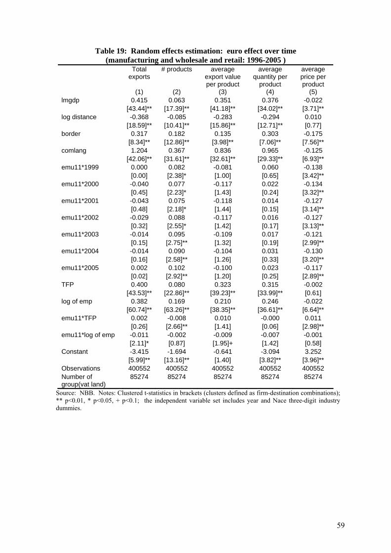
Table 19: Random effects estimation: euro effect over time (manufacturing and wholesale and retail: 1996-2005 )
Total exports
# products average export value per product
average quantity per
product
average price per product
(1) (2) (3) (4) (5) lmgdp 0.415 0.063 0.351 0.376 -0.022 [43.44]** [17.39]** [41.18]** [34.02]** [3.71]** log distance -0.368 -0.085 -0.283 -0.294 0.010 [18.59]** [10.41]** [15.86]** [12.71]** [0.77] border 0.317 0.182 0.135 0.303 -0.175 [8.34]** [12.86]** [3.98]** [7.06]** [7.56]** comlang 1.204 0.367 0.836 0.965 -0.125 [42.06]** [31.61]** [32.61]** [29.33]** [6.93]** emu11*1999 0.000 0.082 -0.081 0.060 -0.138 [0.00] [2.38]* [1.00] [0.65] [3.42]** emu11*2000 -0.040 0.077 -0.117 0.022 -0.134 [0.45] [2.23]* [1.43] [0.24] [3.32]** emu11*2001 -0.043 0.075 -0.118 0.014 -0.127 [0.48] [2.18]* [1.44] [0.15] [3.14]** emu11*2002 -0.029 0.088 -0.117 0.016 -0.127 [0.32] [2.55]* [1.42] [0.17] [3.13]** emu11*2003 -0.014 0.095 -0.109 0.017 -0.121 [0.15] [2.75]** [1.32] [0.19] [2.99]** emu11*2004 -0.014 0.090 -0.104 0.031 -0.130 [0.16] [2.58]** [1.26] [0.33] [3.20]** emu11*2005 0.002 0.102 -0.100 0.023 -0.117 [0.02] [2.92]** [1.20] [0.25] [2.89]** TFP 0.400 0.080 0.323 0.315 -0.002 [43.53]** [22.86]** [39.23]** [33.99]** [0.61] log of emp 0.382 0.169 0.210 0.246 -0.022 [60.74]** [63.26]** [38.35]** [36.61]** [6.64]** emu11*TFP 0.002 -0.008 0.010 -0.000 0.011 [0.26] [2.66]** [1.41] [0.06] [2.98]** emu11*log of emp -0.011 -0.002 -0.009 -0.007 -0.001 [2.11]* [0.87] [1.95]+ [1.42] [0.58] Constant -3.415 -1.694 -0.641 -3.094 3.252 [5.99]** [13.16]** [1.40] [3.82]** [3.96]** Observations 400552 400552 400552 400552 400552 Number of group(vat land)
85274 85274 85274 85274 85274
Source: NBB. Notes: Clustered t-statistics in brackets (clusters defined as firm-destination combinations); ** p<0.01, * p<0.05, + p<0.1; the independent variable set includes year and Nace three-digit industry dummies.
59

Figure 1: Share of trade with EMU11 countries in total EU trade by country (1999=100)
0.85
0.90
0.95
1.00
1.05
1.10
1995 1996 1997 1998 1999 2000 2001 2002 2003 2004
Notes: Non-EMU member countries are plotted as thick line. Greece is the circled line.
60

Figure 2: Product codes at the 8-digits CN level
Entries and exits
-1500
-1000
-500
0
500
1000
1500
1995 1996 1997 1998 1999 2000 2001 2002 2003 2004
Total number of codes
10000
10100
10200
10300
10400
10500
10600
10700
1995 1996 1997 1998 1999 2000 2001 2002 2003 2004
61

Figure 3: Product differentiation and the trade effect of the euro
-1.0
-0.5
0.0
0.5
1.0
1.5
0 1 2 3 4 5 6 7 8
Log number of products
Est
imat
ed E
MU
11 c
oeffi
cien
t
62

Figure 4: Contribution to growth of exports of different margins (1996-2005)
-20%
0%
20%
40%
60%
80%
100%
120%
EZ11 nonEZ3 nonEZeurope nonEZworld
IGZN
Source: NBB. Notes: N is the number of exporters; Z is the average number of products exported by firm, G the average number of destinations at product-firm (variety) level; I is the average value of exports at destination-variety level
63

Figure 5: Components of the extensive margin of exports (base year is 1999)
Number of firms (N)
0
20
40
60
80
100
120
1996 1997 1998 1999 2000 2001 2002 2003 2004 2005
EZ11nonEZ3nonEZeuropenonEZworld
Number of products by firm (Z)
0
20
40
60
80
100
120
140
160
1996 1997 1998 1999 2000 2001 2002 2003 2004 2005
EZ11nonEZ3nonEZeuropenonEZworld
Number of destinations by variety (G)
0
20
40
60
80
100
120
140
160
1996 1997 1998 1999 2000 2001 2002 2003 2004 2005
EZ11nonEZ3nonEZeuropenonEZworld
Source: NBB. Notes: N is the number of exporters; Z is the average number of products exported by firm, G the average number of destinations at product-firm (variety) level; I is the average value of exports at destination-variety level
64

Figure 6: Percentage increase in the predicted probability of exports in 1999 due to the
introduction of the euro
Source NBB. Note: 1 is 100 percent; estimates in Table 14 column were used; top and bottom one percent tails of the productivity distributions dropped.
65

Appendix A
Table A1: Gravity results by chapter Ch. Description Coeff.
14 VEGETABLE PLAITING MATERIALS; VEGETABLE PRODUCTS NOT ELSEWHERE SPECIFIED OR INCLUDED -0.8964
27 MINERAL FUELS, MINERAL OILS AND PRODUCTS OF THEIR DISTILLATION; BITUMINOUS SUBSTANCES; MINERAL WAXES -0.8169
65 HEADGEAR AND PARTS THEREOF -0.7102 *
80 TIN AND ARTICLES THEREOF -0.6201 #
78 LEAD AND ARTICLES THEREOF -0.6064
60 KNITTED OR CROCHETED FABRICS -0.6062 #
50 SILK -0.5893
54 MAN-MADE FILAMENTS; STRIP AND THE LIKE OF MAN-MADE TEXTILE MATERIALS -0.5557 #
8 EDIBLE FRUIT AND NUTS; PEEL OF CITRUS FRUIT OR MELONS -0.4654
97 WORKS OF ART, COLLECTORS' PIECES AND ANTIQUES -0.4651
1 LIVE ANIMALS -0.4195
34
SOAP, ORGANIC SURFACE-ACTIVE AGENTS, WASHING PREPARATIONS, LUBRICATING PREPARATIONS, ARTIFICIAL WAXES, PREPARED WAXES, POLISHING OR SCOURING PREPARATIONS, CANDLES AND SIMILAR ARTICLES, MODELLING PASTES, ‘DENTAL WAXES’ AND DENTAL PREPARATIONS WITH A BASIS OF PLASTER -0.4167
45 CORK AND ARTICLES OF CORK -0.3564
61 ARTICLES OF APPAREL AND CLOTHING ACCESSORIES, KNITTED OR CROCHETED -0.2842 *
86
RAILWAY OR TRAMWAY LOCOMOTIVES, ROLLING STOCK AND PARTS THEREOF; RAILWAY OR TRAMWAY TRACK FIXTURES AND FITTINGS AND PARTS THEREOF; MECHANICAL (INCLUDING ELECTROMECHANICAL) TRAFFIC SIGNALLING EQUIPMENT OF ALL KINDS -0.2439
43 FURSKINS AND ARTIFICIAL FUR; MANUFACTURES THEREOF -0.2139
5 PRODUCTS OF ANIMAL ORIGIN, NOT ELSEWHERE SPECIFIED OR INCLUDED -0.2073
18 COCOA AND COCOA PREPARATIONS -0.1922
23 RESIDUES AND WASTE FROM THE FOOD INDUSTRIES; PREPARED ANIMAL FODDER -0.1787
76 ALUMINIUM AND ARTICLES THEREOF -0.1590
25 SALT; SULPHUR; EARTHS AND STONE; PLASTERING MATERIALS, LIME AND CEMENT -0.1461
62 ARTICLES OF APPAREL AND CLOTHING ACCESSORIES, NOT KNITTED OR CROCHETED -0.1412
87 VEHICLES OTHER THAN RAILWAY OR TRAMWAY ROLLING STOCK, AND PARTS AND ACCESSORIES THEREOF -0.1354
17 SUGARS AND SUGAR CONFECTIONERY -0.1250
31 FERTILISERS -0.1243
94
FURNITURE; BEDDING, MATTRESSES, MATTRESS SUPPORTS, CUSHIONS AND SIMILAR STUFFED FURNISHINGS; LAMPS AND LIGHTING FITTINGS, NOT ELSEWHERE SPECIFIED OR INCLUDED; ILLUMINATED SIGNS, ILLUMINATED NAMEPLATES AND THE LIKE; PREFABRICATED BUILDINGS -0.1209
63 OTHER MADE-UP TEXTILE ARTICLES; SETS; WORN CLOTHING AND WORN TEXTILE ARTICLES; RAGS -0.1114
20 PREPARATIONS OF VEGETABLES, FRUIT, NUTS OR OTHER PARTS OF PLANTS -0.0630
38 MISCELLANEOUS CHEMICAL PRODUCTS -0.0604
42 ARTICLES OF LEATHER; SADDLERY AND HARNESS; TRAVEL GOODS, HANDBAGS AND SIMILAR CONTAINERS; ARTICLES OF ANIMAL GUT (OTHER THAN SILKWORM GUT) -0.0517
35 ALBUMINOIDAL SUBSTANCES; MODIFIED STARCHES; GLUES; ENZYMES -0.0502
55 MAN-MADE STAPLE FIBRES -0.0447
89 SHIPS, BOATS AND FLOATING STRUCTURES -0.0331
39 PLASTICS AND ARTICLES THEREOF -0.0220
22 BEVERAGES, SPIRITS AND VINEGAR -0.0218
83 MISCELLANEOUS ARTICLES OF BASE METAL -0.0049
44 WOOD AND ARTICLES OF WOOD; WOOD CHARCOAL 0.0017
79 ZINC AND ARTICLES THEREOF 0.0051
16 PREPARATIONS OF MEAT, OF FISH OR OF CRUSTACEANS, MOLLUSCS OR OTHER AQUATIC INVERTEBRATES 0.0085
48 PAPER AND PAPERBOARD; ARTICLES OF PAPER PULP, OF PAPER OR OF PAPERBOARD 0.0114
71 NATURAL OR CULTURED PEARLS, PRECIOUS OR SEMI-PRECIOUS STONES, PRECIOUS METALS, METALS CLAD WITH PRECIOUS METAL, AND ARTICLES THEREOF; IMITATION JEWELLERY; COIN 0.0257
49 PRINTED BOOKS, NEWSPAPERS, PICTURES AND OTHER PRODUCTS OF THE PRINTING INDUSTRY; MANUSCRIPTS, TYPESCRIPTS AND PLANS 0.0290
66

56 WADDING, FELT AND NONWOVENS; SPECIAL YARNS; TWINE, CORDAGE, ROPES AND CABLES AND ARTICLES THEREOF 0.0381
72 IRON AND STEEL 0.0419
68 ARTICLES OF STONE, PLASTER, CEMENT, ASBESTOS, MICA OR SIMILAR MATERIALS 0.0446
46 MANUFACTURES OF STRAW, OF ESPARTO OR OF OTHER PLAITING MATERIALS; BASKETWARE AND WICKERWORK 0.0501
53 OTHER VEGETABLE TEXTILE FIBRES; PAPER YARN AND WOVEN FABRICS OF PAPER YARN 0.0725
28 INORGANIC CHEMICALS; ORGANIC OR INORGANIC COMPOUNDS OF PRECIOUS METALS, OF RARE-EARTH METALS, OF RADIOACTIVE ELEMENTS OR OF ISOTOPES 0.0814
12 OIL SEEDS AND OLEAGINOUS FRUITS; MISCELLANEOUS GRAINS, SEEDS AND FRUIT; INDUSTRIAL OR MEDICINAL PLANTS; STRAW AND FODDER 0.0856
74 COPPER AND ARTICLES THEREOF 0.0917
64 FOOTWEAR, GAITERS AND THE LIKE; PARTS OF SUCH ARTICLES 0.1148
3 FISH AND CRUSTACEANS, MOLLUSCS AND OTHER AQUATIC INVERTEBRATES 0.1349
70 GLASS AND GLASSWARE 0.1369
67 PREPARED FEATHERS AND DOWN AND ARTICLES MADE OF FEATHERS OR OF DOWN; ARTIFICIAL FLOWERS; ARTICLES OF HUMAN HAIR 0.1395
73 ARTICLES OF IRON OR STEEL 0.1418
84 NUCLEAR REACTORS, BOILERS, MACHINERY AND MECHANICAL APPLIANCES; PARTS THEREOF 0.1479 #
58 SPECIAL WOVEN FABRICS; TUFTED TEXTILE FABRICS; LACE; TAPESTRIES; TRIMMINGS; EMBROIDERY 0.1650
92 MUSICAL INSTRUMENTS; PARTS AND ACCESSORIES OF SUCH ARTICLES 0.1678
40 RUBBER AND ARTICLES THEREOF 0.1749
52 COTTON 0.1810
96 MISCELLANEOUS MANUFACTURED ARTICLES 0.1896
33 ESSENTIAL OILS AND RESINOIDS; PERFUMERY, COSMETIC OR TOILET PREPARATIONS 0.1898
85
ELECTRICAL MACHINERY AND EQUIPMENT AND PARTS THEREOF; SOUND RECORDERS AND REPRODUCERS, TELEVISION IMAGE AND SOUND RECORDERS AND REPRODUCERS, AND PARTS AND ACCESSORIES OF SUCH ARTICLES 0.1979
51 WOOL, FINE OR COARSE ANIMAL HAIR; HORSEHAIR YARN AND WOVEN FABRIC 0.2016
24 TOBACCO AND MANUFACTURED TOBACCO SUBSTITUTES 0.2097
29 ORGANIC CHEMICALS 0.2115
19 PREPARATIONS OF CEREALS, FLOUR, STARCH OR MILK; PASTRYCOOKS' PRODUCTS 0.2163
69 CERAMIC PRODUCTS 0.2203
13 LAC; GUMS, RESINS AND OTHER VEGETABLE SAPS AND EXTRACTS 0.2323
66 UMBRELLAS, SUN UMBRELLAS, WALKING STICKS, SEAT-STICKS, WHIPS, RIDING-CROPS AND PARTS THEREOF 0.2326
41 RAW HIDES AND SKINS (OTHER THAN FURSKINS) AND LEATHER 0.2346
93 ARMS AND AMMUNITION; PARTS AND ACCESSORIES THEREOF 0.2549
59 IMPREGNATED, COATED, COVERED OR LAMINATED TEXTILE FABRICS; TEXTILE ARTICLES OF A KIND SUITABLE FOR INDUSTRIAL USE 0.3187
57 CARPETS AND OTHER TEXTILE FLOOR COVERINGS 0.3224
37 PHOTOGRAPHIC OR CINEMATOGRAPHIC GOODS 0.3286
21 MISCELLANEOUS EDIBLE PREPARATIONS 0.3434
10 CEREALS 0.3443
95 TOYS, GAMES AND SPORTS REQUISITES; PARTS AND ACCESSORIES THEREOF 0.3446 #
11 PRODUCTS OF THE MILLING INDUSTRY; MALT; STARCHES; INULIN; WHEAT GLUTEN 0.3711
81 OTHER BASE METALS; CERMETS; ARTICLES THEREOF 0.3926
15 ANIMAL OR VEGETABLE FATS AND OILS AND THEIR CLEAVAGE PRODUCTS; PREPARED EDIBLE FATS; ANIMAL OR VEGETABLE WAXES 0.4013
30 PHARMACEUTICAL PRODUCTS 0.4073
82 TOOLS, IMPLEMENTS, CUTLERY, SPOONS AND FORKS, OF BASE METAL; PARTS THEREOF OF BASE METAL 0.4096 #
32 TANNING OR DYEING EXTRACTS; TANNINS AND THEIR DERIVATIVES; DYES, PIGMENTS AND OTHER COLOURING MATTER; PAINTS AND VARNISHES; PUTTY AND OTHER MASTICS; INKS 0.4207
90 OPTICAL, PHOTOGRAPHIC, CINEMATOGRAPHIC, MEASURING, CHECKING, PRECISION, MEDICAL OR SURGICAL INSTRUMENTS AND APPARATUS; PARTS AND ACCESSORIES THEREOF 0.4331 *
7 EDIBLE VEGETABLES AND CERTAIN ROOTS AND TUBERS 0.4462
2 MEAT AND EDIBLE MEAT OFFAL 0.4534
91 CLOCKS AND WATCHES AND PARTS THEREOF 0.4633
4 DAIRY PRODUCE; BIRDS' EGGS; NATURAL HONEY; EDIBLE PRODUCTS OF ANIMAL ORIGIN, NOT ELSEWHERE SPECIFIED OR INCLUDED 0.4763 #
98 COMPLETE INDUSTRIAL PLANT 0.5103
67

9 COFFEE, TEA, MATÉ AND SPICES 0.5737
6 LIVE TREES AND OTHER PLANTS; BULBS, ROOTS AND THE LIKE; CUT FLOWERS AND ORNAMENTAL FOLIAGE 0.5780 *
36 EXPLOSIVES; PYROTECHNIC PRODUCTS; MATCHES; PYROPHORIC ALLOYS; CERTAIN COMBUSTIBLE PREPARATIONS 0.6010
47 PULP OF WOOD OR OF OTHER FIBROUS CELLULOSIC MATERIAL; RECOVERED (WASTE AND SCRAP) PAPER OR PAPERBOARD 0.6696
88 AIRCRAFT, SPACECRAFT, AND PARTS THEREOF 0.7158 #
75 NICKEL AND ARTICLES THEREOF 0.7295
26 ORES, SLAG AND ASH 1.0167 *
Notes: Dependent variable is the log of imports. The specification is similar to the benchmark specification in column 1 of Table 3. Standard errors (robust to clustering by country-pairs) are in parentheses. **, * and # denotes significant at the 1, 5 and 10 percent level, respectively.
68


