
Sequential Resource Allocation Schemes in
Wireless Mesh Networks
Jae-Ryong Cha
School of Electrical and Computer Engineering
Ajou University
February, 2013


Abstract
Wireless mesh networks (WMNs) are emerging communica-
tion networks consisting of nodes that automatically establish
an ad-hoc network and maintain mesh connectivity. With
the popularity of WMNs, supporting quality of service (QoS)
over multihop radio links is becoming an important issue be-
cause end-to-end (ETE) delay increases quickly with the in-
crease in the number of hops. Various QoS-aware scheduling
schemes based on time division multiple access (TDMA) have
been proposed for supporting a variety of applications such
as voice and video calls in multihop WMNs. Basically, they
have been focusing on determining minimum length sched-
ules. Although such schemes reduce a frame length, they
may bring about queuing delay which can increase ETE de-
lay because they share a slot for multiple flows in a link.
Meanwhile, the order of timeslots scheduled in a flow also
may have an effect on ETE delay in multihop WMNs. Some
papers have proposed scheduling schemes considering the or-
der of timeslots. However, they all have assumed that there
is always a centralized station in a network. Recently, many

researches on network coding (NC) scheme have been intro-
duced to increase the utilization of valuable resources in mul-
tihop WMNs. So far, almost all conventional works on NC
have focused on the improvement of network throughput ef-
ficiency that is the original objective of NC. However, if an
appropriate link schedule for NC is not considered, ETE delay
may be increased even though NC gain can be obtained.
Therefore, this dissertation first proposes a fully-distributed
resource allocation scheme called sequential link schedule (SLS)
that not only eliminates queueing delay but also considers the
order of timeslots scheduled on a path. In the proposed SLS
scheme, channel locking algorithm called time slot acquisi-
tion (TSA) is employed for interference free slot allocation
in a distributed manner. Then, the multihop slot allocation
(MSA) algorithm is carried out to sequentially allocate slots
on the path. According to the analysis results, in case of
deterministic packet arrival, the proposed SLS scheme shows
shorter ETE delay, even though it starts the packet transmis-
sion with slightly greater frame length than that in case of the
minimum length schedule (MLS). For the non-deterministic
packet arrival having exponential distribution, the proposed
SLS scheme shows a slightly lower delay performance. How-
ever, the proposed SLS scheme is more tolerable for a high
packet interarrival rate than the MLS. In the next proposal,
two bandwidth allocation schemes jointly combined with NC
are proposed to reduce ETE delay and enhance resource uti-
lization in the network. The first proposed section-based se-
quential scheduling scheme, which is flow-based one, employs
a new concept, ‘section’, so that the slots scheduled on a path
are sequentially arranged within a frame even when NC oper-
ation is performed. The second proposed scheme is a ‘dupli-
cated allocation followed by resource release’ (DARR) based
sequential scheduling scheme. The basic idea of the proposed
DARR-based scheme is that, when the MSA algorithm has
been initiated from the non-reference NC flow, an NC coordi-
nator not only transfers an slot allocation (SA) packet to the
next node of the non-reference NC flow but also again trans-
fers another SA packet to the next node of reference NC flow
before releasing the initially-allocated slots. By the simula-
tion results, it is known that the proposed schemes show bet-
ter delay performance than the conventional SLS-NC. There-
fore, by applying the conventional XOR-based NC scheme to
the link scheduling, the proposed schemes give more delay-
efficient slot assignments that result in better channel uti-
lization while at the same time using less network resources
and energy. In conclusion, the proposed sequential scheduling
schemes can give the sequentiality with NC gain guaranteed,
thereby resulting in decreasing ETE delay and enhancing the
resource utilization in multihop WMNs.

vi

Contents
List of Figures iii
List of Tables vii
Abbreviation ix
1 Introduction 1
1.1 Background and Motivation . . . . . . . . . . . . . . . . 1
1.2 Contributions . . . . . . . . . . . . . . . . . . . . . . . . 4
2 Related Work 7
2.1 Scheduling in WMNs . . . . . . . . . . . . . . . . . . . . 7
2.2 Network Coding . . . . . . . . . . . . . . . . . . . . . . . 11
3 System Model 23
4 Sequential Scheduling in TDMA-based WMNs 27
4.1 Motivation . . . . . . . . . . . . . . . . . . . . . . . . . . 27
4.2 Proposed SLS Scheme . . . . . . . . . . . . . . . . . . . 34
4.2.1 TSA algorithm . . . . . . . . . . . . . . . . . . . 38
i

4.2.2 MSA algorithm . . . . . . . . . . . . . . . . . . . 40
4.2.3 Performance analysis . . . . . . . . . . . . . . . . 42
4.2.4 Performance evaluation . . . . . . . . . . . . . . . 49
4.2.5 Numerical and simulation results . . . . . . . . . 52
4.3 Summary . . . . . . . . . . . . . . . . . . . . . . . . . . 59
5 Sequential Scheduling jointly combined with NC in TDMA-
based WMNs 61
5.1 Motivation . . . . . . . . . . . . . . . . . . . . . . . . . . 64
5.2 Proposed Section-based Scheme . . . . . . . . . . . . . . 66
5.2.1 Performance analysis . . . . . . . . . . . . . . . . 76
5.3 Proposed DARR-based Scheme . . . . . . . . . . . . . . 78
5.3.1 Performance analysis . . . . . . . . . . . . . . . . 82
5.4 How to Cope with Asymmetric Flow Conditions . . . . . 83
5.5 Performance Evaluation . . . . . . . . . . . . . . . . . . 85
5.6 Numerical and Simulation Results . . . . . . . . . . . . . 91
5.7 Summary . . . . . . . . . . . . . . . . . . . . . . . . . . 102
6 Conclusion 103
References 107
ii

List of Figures
1.1 Example of a WMN . . . . . . . . . . . . . . . . . . . . 2
2.1 Scheduling in terms of an integrated problem. . . . . . . 8
2.2 Classification framework for scheduling schemes. . . . . . 9
2.3 Example of X constellation with opportunistic listening. 11
2.4 Example of other NC constellations. . . . . . . . . . . . . 15
3.1 Frame structure in DCH . . . . . . . . . . . . . . . . . . 23
4.1 QPs in multihop wireless networks. . . . . . . . . . . . . 28
4.2 Topology of a four-node network. . . . . . . . . . . . . . 30
4.3 Example of an RLS. . . . . . . . . . . . . . . . . . . . . 30
4.4 Example of an SLS. . . . . . . . . . . . . . . . . . . . . . 30
4.5 Delay components of an RLS. . . . . . . . . . . . . . . . 31
4.6 Delay effect by an allocation order. . . . . . . . . . . . . 33
4.7 Information on some terminologies used for the MSA al-
gorithm. . . . . . . . . . . . . . . . . . . . . . . . . . . . 34
4.8 State diagram for the TSA algorithm. . . . . . . . . . . . 36
4.9 Example of a failed round. . . . . . . . . . . . . . . . . . 37
iii

4.10 Example of a successful round. . . . . . . . . . . . . . . . 37
4.11 Delay components of the proposed SLS scheme. . . . . . 47
4.12 Example of TS−D calculation. . . . . . . . . . . . . . . . 49
4.13 ETE delay with different traffic load and TX power: DPA. 56
4.14 ETE delay with different traffic load and TX power: NDPA. 57
5.1 NC constellations for scheduling . . . . . . . . . . . . . . 62
5.2 Delay effect in an RLS with NC: case 1 . . . . . . . . . . 63
5.3 Delay effect in an RLS with NC: case 2 . . . . . . . . . . 63
5.4 Example of an SLS with NC . . . . . . . . . . . . . . . . 63
5.5 Example of the slot allocation when h(i)= 2 and 4 for four
sections . . . . . . . . . . . . . . . . . . . . . . . . . . . 67
5.6 Example of the slot allocation when h(i)= 4 and 3 for four
sections . . . . . . . . . . . . . . . . . . . . . . . . . . . 67
5.7 NC condition 1: x(ei) = x(gj) . . . . . . . . . . . . . . . 70
5.8 NC condition 2: x(ei) = x(gj) + 1 . . . . . . . . . . . . . 70
5.9 NC condition 3: x(ei) = x(gj) - 1 . . . . . . . . . . . . . 70
5.10 NC condition 4: x(ei) < x(gj) - 1 or x(ei) > x(gj) + 1 . 70
5.11 Examples of the proposed DARR-based scheme. . . . . . 81
5.12 Example network where an asymmetric flow condition oc-
curs. . . . . . . . . . . . . . . . . . . . . . . . . . . . . . 84
5.13 ETE delay in DPA case: No errors. . . . . . . . . . . . . 94
5.14 ETE delay in DPA case: 0 dBm of TX power. . . . . . . 95
5.15 ETE delay in DPA case: -1 dBm of TX power. . . . . . . 96
5.16 ETE delay in DPA case: -2 dBm of TX power. . . . . . . 97
iv
5.17 ETE delay in NDPA case: No errors. . . . . . . . . . . . 98
5.18 ETE delay in NDPA case: 0 dBm of TX power. . . . . . 99
5.19 ETE delay in NDPA case: -1 dBm of TX power. . . . . . 100
5.20 ETE delay in NDPA case: -2 dBm of TX power. . . . . . 101
v

vi

List of Tables
2.1 Comparison of conventional works: Scheduling . . . . . . 12
2.2 Comparison of conventional works: Scheduling (con’t) . . 13
2.3 Comparison of conventional works: NC . . . . . . . . . . 18
2.4 Comparison of conventional works: NC (con’t) . . . . . . 19
2.5 Comparison of conventional works: NC (con’t) . . . . . . 20
2.6 Comparison of conventional works: NC (con’t) . . . . . . 21
4.1 Field size of packets used for the proposed MSA algorithm 35
4.2 Preliminary results . . . . . . . . . . . . . . . . . . . . . 51
4.3 Parameters for overhead calculation . . . . . . . . . . . . 52
4.4 MSA overhead: power consumption . . . . . . . . . . . . 53
4.5 MSA overhead: Routing and SA time . . . . . . . . . . . 53
4.6 Preliminary results in the MLS . . . . . . . . . . . . . . 54
5.1 Lists and brief explanations of scheduling schemes for the
performance comparison. . . . . . . . . . . . . . . . . . . 87
5.2 Parameters and preliminary results . . . . . . . . . . . . 89
5.3 Overhead comparison: power consumption (Joules) . . . 90
vii

5.4 Average coding gain in the network . . . . . . . . . . . . 91
viii

Abbreviation
ACK acknowledgement
AODV adhoc on-demand distance vector
AP access point
BFS bottleneck first scheduling
BS base station
CAC call admission control
CBR constant bit rate
CCH common channel
CSLS conventional sequential link scheduling
CSMA carrier sensing multiple access
DARR duplicate allocation followed by resource release
DCH data channel
DPA deterministic packet arrival
ix

EDF earlier deadline first
ETE end-to-end
FCFS first come first serve
GF(2) galois field of two elements
GFLS global frame length synchronization
ID identification
IEEE institute of electrical and electronics engineers
IFLS initial frame length synchronization
ILP integer linear programming
IP internet protocol
LP linear programming
MAC medium access control
MBS mesh base station
MLS minimum length schedule
MSA multihop slot allocation
NC network coding
NDPA non-deterministic packet arrival
OFDM orthogonal frequency division multiplexing
OFDMA orthogonal frequency division multiple access
x

PHY physical
PMP point to multi-point
QoS quality of service
QP queuing point
RAV Reception AVailable
RLS random link scheduling
SA slot allocation
SLS sequential link scheduling
SS subscriber stations
TAV Transmission AVailable
TDMA time division multiple access
TRAV Transmission/Receiption AVailable
TSA time-slot acquisition
TX transmission
UAV UnAVailable
UWB ultra wide band
WBN wireless backbone network
WiFi wireless fidelity
WiMAX worldwide interoperability for microwave access
xi

WLAN wireless local area network
WMN wireless mesh network
xii

1
Introduction
1.1 Background and Motivation
Recent years have witnessed the emergence of a variety of wireless services
such as video conferencing, IP TV, music downloading, and online gam-
ing. Motivated by the concept of ubiquitous computing, these wireless
services are designed to be available for people anytime and anywhere.
WMNs have been considered as a promising technology which can sup-
port these kinds of services because of the future needs for seamless and
cheap connectivity. The core idea of WMNs is that multiple nodes col-
laborate to form a wireless backbone which can then be used to route
packets from source nodes to destination nodes possibly via multiple
hops. It also enables users to connect to a node on the backbone of the
WMN, and then access the resources presented by the WMN backbone
to communicate with other nodes on the WMN. In addition, if any node
in the WMN backbone happens to have access to the Internet via wired
1
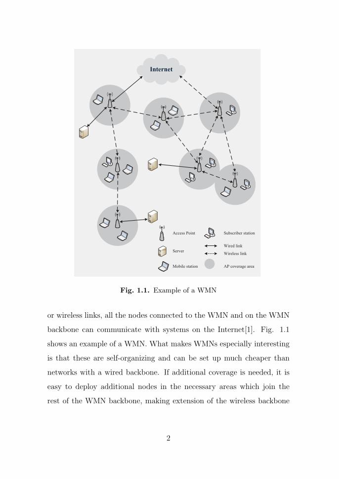
Internet
Access Point
Server
Subscriber station
Wired link
Wireless link
Mobile station AP coverage area
Fig. 1.1. Example of a WMN
or wireless links, all the nodes connected to the WMN and on the WMN
backbone can communicate with systems on the Internet[1]. Fig. 1.1
shows an example of a WMN. What makes WMNs especially interesting
is that these are self-organizing and can be set up much cheaper than
networks with a wired backbone. If additional coverage is needed, it is
easy to deploy additional nodes in the necessary areas which join the
rest of the WMN backbone, making extension of the wireless backbone
2

very flexible. Given these benefits, the IEEE 802.16 standard[2] intro-
duces an additional and optional MeSH mode of operation in addition
to the PMP mode of operation. In this mode, nodes in the network can
communicate with each other and the base station via routing packets
over multiple hops. In contrast to the MeSH mode of operation currently
being standardized by the IEEE 802.16 working group, the MeSH mode
supports topologies which need not have to be a strictly tree topology
rooted at the BS. WMNs are also being followed by interest within the
IEEE 802.11 working group which has led to the working group 802.11s.
IEEE 802.11s is concerned with extensions to the IEEE 802.11 standard
to enable efficient setup of WMNs using the 802.11 standard. The goal
here is to be able to connect nearby mobile devices (e.g., laptops) to
form a local mesh network which may or may not provide access to the
Internet. WMNs are also seen as a promising approach to setup flexible
industrial sensor networks for factory/process automation. The Wireless
HART standard[3] supports the setup of wireless mesh topologies for the
application scenarios of these networks. Many universities (Roofnet[4],
QuRiNet[5], Fractel[6], Lo3[7]), as well as industrial labs (VillageNet[8])
have on-going research projects on various aspects of mesh networking
and several technology leaders (Firetide[9]) and startups are building
mesh networking platforms and deploying services for communication
and data transfer[10].
However, although WMNs can support various wireless services with
seamless and cheap connectivity, the bandwidth in such networks still re-
mains a scarce resource. Recently, network coding has been investigated
3
as a novel mechanism to permit the saving of valuable bandwidth in
such WMNs for individual transmissions, thereby increasing the traffic-
carrying capacity of WMNs. Up-to-date, the practical investigations for
the deployment of network coding have been limited to WMNs based on
the IEEE 802.11 standard. There have been no significant investigations
on the deployment of network coding, and its benefits in TDMA-based
multihop WMNs. Given the fact that the next generation of WMNs
would be using bandwidth reservation schemes to support realtime appli-
cations such as advanced multimedia services and video conferencing, it
is vital that network coding be investigated in the light of such WMNs to
meet QoS requirements. Specifically, we formulate a general framework,
which is applicable to any transmission schemes with or without NC,
to increase the resource utilization and decrease ETE delay in TDMA-
based multihop WMNs. Our framework features to support stringent
QoS requirements (e.g., delay bound) with NC gain guaranteed. Un-
der this developed framework, we propose joint link scheduling and NC
schemes. We also perform extensive simulations to validate and evaluate
the performance of our proposed schemes.
1.2 Contributions
With the popularity of WMNs, supporting QoS over multihop radio links
is a critical issue because ETE delay is quickly increased with the increase
in the number of hops. Meanwhile, although WMNs can support various
wireless services with seamless and cheap connectivity, the bandwidth in
4

such networks still remains a scarce resource. Recently, many researches
have been performed on NC to increase the utilization of valuable re-
sources in WMNs. However, if an appropriate link scheduling for NC is
not performed, ETE delay may be increased although NC gain can be
obtained. Therefore, when designing a scheduling scheme in WMNs, con-
sidering these two factors (i.e., ETE delay and scarce resources) is very
important in order to support QoS and increase resource utilization. Un-
der this necessity, there are several contributions in this dissertation as
follows:
• General framework for fully-distributed sequential schedule was
presented. This makes it possible to sequentially allocate slots on
the path in a flow without collision, resulting in reducing ETE delay
in multihop WMNs;
• Two sequential scheduling schemes jointly combined with NC were
presented. The proposed schemes can not only get the same NC
gain as the conventional scheme but also guarantee the sequentiality
with small overhead, thereby resulting in decreasing ETE delay in
multihop WMNs;
• Simple scheme to cope with asymmetric flow conditions was pre-
sented. This prevents one flow related to NC from waiting for
another flow, ultimately resulting in no additional delay caused by
NC operation.
5

6

2
Related Work
The goal of this section is to introduce in brief the readers of this disser-
tation to the work in the literature which is closely related to the work in
this dissertation as well as associated concepts. The scheduling and its
related conventional works in WMNs are first introduced and the basic
concept of NC and the requirements for NC to be used in TDMA are
described.
2.1 Scheduling in WMNs
Recently, wireless mesh networking has emerged as an interesting and
challenging area of research. It is attracting significant interest to sup-
port ubiquitous communication and broadband access using low-cost net-
working platforms. Essentially, nodes in a wireless network have the mesh
capability, wherein the nodes not only transmit local data but also sup-
port flows of other mesh nodes through them, thus forming a multihop
7
RoutingChannel
Assignment
Link Scheduling
QoS
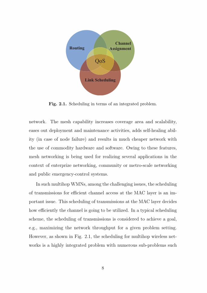
Fig. 2.1. Scheduling in terms of an integrated problem.
network. The mesh capability increases coverage area and scalability,
eases out deployment and maintenance activities, adds self-healing abil-
ity (in case of node failure) and results in much cheaper network with
the use of commodity hardware and software. Owing to these features,
mesh networking is being used for realizing several applications in the
context of enterprize networking, community or metro-scale networking
and public emergency-control systems.
In such multihopWMNs, among the challenging issues, the scheduling
of transmissions for efficient channel access at the MAC layer is an im-
portant issue. This scheduling of transmissions at the MAC layer decides
how efficiently the channel is going to be utilized. In a typical scheduling
scheme, the scheduling of transmissions is considered to achieve a goal,
e.g., maximizing the network throughput for a given problem setting.
However, as shown in Fig. 2.1, the scheduling for multihop wireless net-
works is a highly integrated problem with numerous sub-problems such
8

Scheduling
Problem setting Goals Inputs Techniques
Fig. 2.2. Classification framework for scheduling schemes.
as how to find optimal routing path, how to assign optimal channel to
the network, and how to perform interference-free link activation for the
optimal link scheduling[10]. Several of these sub-problems, e.g. optimal
channel assignment, are proven NP-hard problems[11] and thus the over-
all problem of scheduling is necessarily complex. In addition, application
constraints like providing quality of service is also one of the important
aspects that scheduling has to take into account. Given a problem set-
ting and a set of inputs, scheduling transmissions in multihop WMNs is
about employing a technique to allocate time and channel (frequency)
resources to mesh nodes/links to achieve a set of goals.
Fig. 2.2 shows classification framework for scheduling in multihop
mesh networks based on problem settings, goals, inputs, and techniques.
The first dimension of the classification framework, ‘Problem setting’,
classifies a scheduling mechanism based on types of scheduling controls,
types of channel access protocol, antenna type and types of network
topologies considered. The type of scheduling control can be centralized,
where a central node takes the scheduling decisions, or distributed where
the set of network nodes mutually converge on a schedule. The type
9
of channel access protocol can be either CSMA or TDMA. Particularly,
WiMAX mesh standard employs a TDMA based multihop mesh proto-
col. Next, antenna type can be either omni-directional, directional or
sector antenna. Network topology can be further classified into tree or
graph. Tree topology is prominently considered in several WiMAX mesh
scheduling mechanisms. However, in general, scheduling mechanisms for
multihop wireless mesh consider a generic graph as the underlying net-
work topology. The second dimension, ‘Goals’, classifies a scheduling
mechanism based on the goals of the problem. One of goals in a schedul-
ing mechanism is to schedule the resources to maximize the throughput
of the network. Other goals include scheduling to maximize number of
flows admitted, scheduling to satisfy minimum bandwidth requirement
of each flow and scheduling to satisfy strict constraints like delay and
jitter for real-time applications. The third dimension, ‘Inputs’, classifies
a scheduling mechanism based on the types of inputs considered for the
problem. A scheduling mechanism considers a subset of inputs from: (1)
number of channels available for scheduling, (2) number of radios present
at the mesh nodes, (3) ETE flow requirements of the flows (e.g., data
rate), (4) routing paths provided for the flows, (5) interference map spec-
ifying conflicts in link scheduling, (6) channel-state information, and (7)
quality of service parameters (e.g., minimum and maximum capacities
on data rates). The fourth important dimension, ‘Techniques’ decides
the effectiveness of scheduling mechanisms. The types of techniques are
mostly driven by the problem setting and goal of scheduling mechanism.
The stricter the goal gets, the harder the scheduling technique becomes.
10

Pa
R
Pb
Sb Sa
x1 y1
x1 y1 x1 y1
1 2 3 4 5 6 7 8
x1 y1 z1
1 2 3 4 5 6 7 8
Pa
R
Pb
Sb Sa
x1 y1
x1
x1
y1
y1
x1 y1
z1
Fig. 2.3. Example of X constellation with opportunistic listening.
As mentioned earlier, the NP-hard sub-problems make the scheduling
problem even more “complex”. Typically, the scheduling problem is for-
mulated as an ILP and the relaxed LP is solved to approximate the
solution. Other techniques include max-flow based algorithms, heuristics
(greedy algorithms), and algorithms using graph properties. Table 2.1
and 2.2 summarize the comparison of conventional works according to
a subset along both scheduling algorithms and classification dimensions
based on the classification framework explained[10].
2.2 Network Coding
NC is becoming an emerging communication paradigm that can provide
the performance improvement in throughput and energy efficiency. NC
was originally proposed for wired networks, and the throughput gain
was illustrated by the well-known example of “butterfly” network[24].
11

Table
2.1.Com
parison
ofcon
vention
alworks:
Schedulin
g
Work
sSchedule
control
Top
ologiesMulti-ch
annel/rad
ioSchedulin
ggoal
JR-M
CMR[12]
Centralized
Grap
hYes/Y
esFair
allocation
ofwireless
resources
C-W
iMAX[13]
Centralized
Tree
No/Y
esInterferen
ce-freerou
te
computation
A-W
iMAX[14]
Centralized
Tree
Yes/N
oTo
satisfyminim
um
ban
dwidth
and
max
-
imum
allowed
delay
requirem
ents
oftheflow
s
Delay
Aware[15]
Centralized
graph
No/N
oTofindminim
um
length
schedule
tominim
ize
ETEsch
edulin
gdelay
Delay
Back
hau
l[16]Centralized
Tree
Yes/N
oLinkactivation
schedule
tobou
ndETEdelay
CACQoS
[17]Centralized
Grap
hNo/N
oInterferen
ce-freerou
te
computation
12

Table
2.2.Com
parison
ofconvention
alworks:
Scheduling(con
’t)
Works
Schedule
control
Top
ologies
Multi-chan
nel/rad
ioSchedulinggoal
Rou
tingR
ural[18]
Centralized
Graph
No/No
Interference-free
route
computation
Chan
nelRural[19]
Centralized
Graph
Yes/Y
esInterference-free
route
computation
Lon
gTDMA[20]
Centralized
Tree
yes/No
Interference-free
and
delay-aware
route
com-
putation
DelayCheck[21]
Centralized
Graph
yes/Yes
Max
imizethenumber
of
voicecallsscheduled
DRAND[22]
Distributed
Graph
No/No
Interference-free
route
computation
CodeP
lay[23]
Distributed
Graph
No/No
Schedule
realtime
flow
s
indynam
icmesh
topol-
ogy
13

Recently, there is a growing interest to apply NC onto wireless networks
since the broadcast nature of wireless channel makes NC particularly
advantageous in terms of bandwidth efficiency and enables opportunistic
encoding and decoding[25]. NC makes it possible for an intermediate
node to combine packets it has received or generated itself such that one
or more outgoing packets can be forwarded to the other nodes. Fig. 2.3
shows the well-known ‘X constellation’ for NC, which is composed of two
predecessor nodes Pa and Pb, an NC coordinator R, and two successor
nodes Sa and Sb. In Fig. 2.3, the solid line means unicasting transmission
and other lines mean broadcasting transmission. As shown in Fig. 2.3,
Pa has a packet x1 for Sa, and Pb has a packet y1 for Sb. The two packets
from both flows have to be relayed via R. In conventional slot scheduling,
four transmissions (four slots) are necessary to accomplish the delivery of
two packets (x1 and y1) as shown in Fig. 2.3(left). However, if using NC,
three transmission (three slots) are necessary to deliver the two packets
as shown in Fig. 1(right): i.e.,
• Pa broadcasts packet x1 to R and Sb in the 2nd slot;
• Pb broadcasts packet y1 to R and Sa in the 3rd slot;
• R broadcasts z1 (x1 ⊕ y1) to Sb and Sa in the 5th slot.
From the above example, by using this baseline NC scheme, the num-
ber of transmissions (slots) can be reduced; as a result, the network
throughput efficiency can be increased. NC also can be used in case of
no opportunistic listening[25], and one of these scenarios is presented in
14

Pa PbR
(2)(1)
(3)(3)
x1 y1
Pa
S
R
Pb
(3) (2)
(1)
(3)
x1
y1
Fig. 2.4. Example of other NC constellations.
Fig. 2.4(left). In Fig. 2.4, the solid line means unicasting transmission
and other lines mean broadcasting transmission. In this case, the source
node Pa needs to send a packet x1 to node Pb (1) and another source
node Pb needs to send a packet y1 to node Pa (2). Since each source is
also a destination node, it has the necessary packets for decoding upon
receiving the encoded packet x1⊕y1 from the NC coordinator R (3). Fig.
2.4(right) shows a hybrid scenario where node Pa needs no opportunistic
listening and the successor node S needs the opportunistic listening from
node Pb. In this case, the source node Pa needs to send a packet x1 to node
S (1). And, another source node Pb needs to send a packet y1 to node Pa
(2). At this time, node Pb broadcasts the packet y1 for the overhearing
of node S (2). After the broadcasting of the encoded packet (x1⊕y1) by
the NC coordinator R, Pa decodes the packet y1 (x1⊕(x1⊕y1)) using its
packet x1. On the other hand, S decodes the packet x1 (y1⊕(x1⊕y1))
using the packet y1 overheard from Pb. In both cases, instead of four
packet transmissions when NC is not used, only three transmissions are
necessary, thereby reducing the bandwidth utilization. As seen from the
15

example, we can see that NC is able to increase the effective information
transfer rate beyond the physical capacity (data transfer rate) which is
provided by the network. We define an NC set as five nodes constructing
an X constellation in Fig. 2.3, three nodes constructing a string constel-
lation in Fig. 2.4(left), or four nodes constructing a hybrid constellation
in Fig. 2.4(right). For example, at the X constellation as shown in Fig.
2.3, the criteria for the NC set are as follows:
• Pa is beyond the communication range of Pb;
• Sa is beyond the communication range of Sb;
• Sb must overhear the packets from Pa;
• Sa must overhear the packets from Pb.
However, most of the conventional works have been only theoretical
in nature and restricted to the case of application of NC to multicast
traffics. There has also been some work looking into the case of appli-
cation of NC to unicast transmissions in networks[26],[27]. In case of a
single unicast or broadcast session, the authors in [28] showed that there
are no improvements over routing obtainable as far as throughput is con-
cerned when NC is used. In case of multiple unicast transmissions, the
authors in [27] showed that NC can be beneficial compared to routing.
However, the benefit is strongly dependent on the network topology and
the authors [27] conjecture that, for undirected networks with fractional
routing, the potential for NC to increase bandwidth efficiency does not
exist. For the multiple unicast transmissions case, the authors in [29]
16

showed that NC does not provide any order difference improvement over
the bound provided by the work[30] which does not consider NC. Similar
results are presented by [31] for the case of multicast traffic. However,
in [32] and [33], the authors showed that NC does bring a constant fac-
tor gain over routing for the multiple unicast as well as multicast traffic
cases in wireless networks. This gain is very valuable in practice as it
means a direct increase in the traffic which can be supported by the
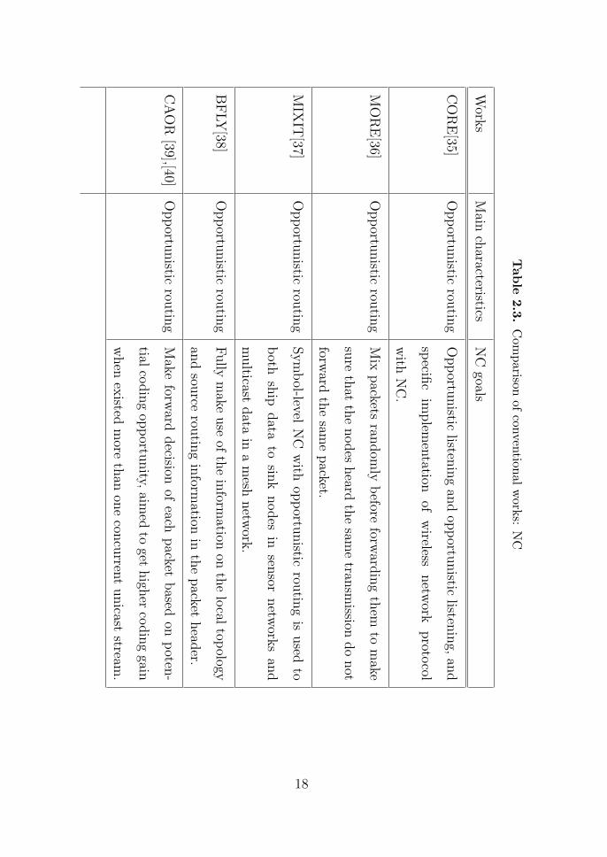
network[34]. Table 2.3 through 2.6 list the conventional works on NC
in terms of opportunistic routing, security, retransmission strategy, and
relay communication.
17
Table
2.3.Com
parison
ofcon
vention
alworks:
NC
Work
sMain
characteristics
NC
goals
CORE[35]
Opportu
nistic
routin
gOpportu
nistic
listeningan
dop
portu
nistic
listening,
and
specifi
cim
plem
entation
ofwireless
netw
orkproto
col
with
NC.
MORE[36]
Opportu
nistic
routin
gMix
packets
random
lybefore
forward
ingthem
tomake
sure
that
thenodes
heard
thesam
etran
smission
donot
forward
thesam
epacket.
MIX
IT[37]
Opportu
nistic
routin
gSymbol-level
NC
with
opportu
nistic
routin
gis
used
to
both
ship
data
tosin
knodes
insen
sornetw
orksan
d
multicast
data
inamesh
netw
ork.
BFLY[38]
Opportu
nistic
routin
gFully
make
use
oftheinform
ationon
thelocal
topology
andsou
rcerou
tinginform
ationin
thepacket
head
er.
CAOR
[39],[40]Opportu
nistic
routin
gMake
forward
decision
ofeach
packet
based
onpoten
-
tialcodingop
portu
nity,
aimed
toget
high
ercodinggain
when
existed
more
than
onecon
curren
tunicast
stream.
18

Table
2.4.Com
parison
ofconvention
alworks:
NC
(con’t)
Works
Maincharacteristics
NC
goal
OCR[41]
Opportunisticrouting
Mainly
studiedhow
toim
prove
thedatatran
smission
perform
ance
inW
MNsbycombinationof
opportunistic
routingan
dNC.
ONCC[42]
Opportunisticrouting
Opportunisticnetwork
coded
coop
eration
schem
efor
multiple
unicasttran
smission
pairs
inasinglecellwire-
less
networks.
Pollution
[43]
Security
research
NC
methodwhichcandetecttheexistence
ofpollution
attack.
SecureNC[44]
Security
research
Adap
tive
secure
NC
forthedifference
inab
ilityof
the
attacker.
Wiretab
[45]
Security
research
Design
asecure
NC
model
nam
edwiretap
network
,whichcanincorporateinform
ationsecurity
withNC.
Cap
acity[46]
Security
research
Givethelimitationof
multicastcapacitywiththesecu-
rity.
19

Table
2.5.Com
parison
ofcon
vention
alworks:
NC
(con’t)
Work
sMain
characteristics
NC
goal
Privacy
[47]Secu
rityresearch
Prop
oseanovel
privacy
-preserv
ingsch
emeagain
sttraf-
fican
alysis
attacksin
NC.
Sign
ature[48]
Secu
rityresearch
Prop
oseasign
ature-b
asedsch
emeagain
stpollu
tionat-
tacksfor
securin
glin
earNC.
NullK
ey[49]
Secu
rityresearch
Secu
ritysch
emefor
NC
that
does
not
require
large
computation
s,nor
addan
yred
undan
cyto
theorigin
al
blocks.
Secu
rity[50]
Secu
rityresearch
Analy
zehow
toim
prove
security
with
NC
inW
MNs.
Com
bined[51]
Retran
smission
based
Prop
osetw
ostrategies
combined
ofNC
andretran
smis-
sion
GF[52]
Retran
smission
based
Inthefield
GF(2),
findtheprob
lemof
wireless
packet
retransm
issionpacket
retransm
issionstrategy
forat
leastaNPC
prob
lem
20

Table
2.6.Com
parison
ofconvention
alworks:
NC
(con’t)
Works
Maincharacteristics
NC
goal
NCW
BR[53]
Retransm
ission
based
Inwirelessbroad
casting,
combinethedifferentlostpack-
etswithNC
forretran
smission
.
combination[54],[55]
Relay
communication
Givethecombinationdesignschem
ewithchan
nel
cod-
ingan
dNC
Security[56]
Relay
communication
Proposean
NC
fram
eworkforwirelessrelaynetworks
which
took
thefadingan
derrorpronenature
ofthe
wirelessnetworksinto
consideration.
Joint[57]
Relay
communication
ProposeajointNC
and
superposition
codingschem
e
forinform
ationexchan
gebetweenmorethan
twousers
inawirelessrelayingnetworkto
exchan
geinform
ation
betweenmorethan
twosourcenodes
infewer
timeslots.
GF[58]
Relay
communication
ProposeaAnalog
NetworkCodingmethodwhichcan
carrymultiple
messagesin
sign
alin
physicallayer.
21

22

3
System Model
In this dissertation, we model WMNs with a topology graph connecting
the nodes that are present in each other’s wireless range. The network
can be represented with a directed connectivity graph G(B,E), where
B = {b1, ..., bm} is a set of nodes and E = {e1, ..., eg} is a set of directed
links, and two nodes (u and v) are neighbors if (u, v) ∈ E. In the
network, F is a set of flows, and a flow f(∈ F ) is specified by a node
set R(f) = {p1, ..., pq}, where pk is the kth node in a flow (2 ≤ q; k = 1:
the source node, 1 < k < q: the intermediate node(s), and k = q: the
destination node). We consider free space path loss and slow fading
channel. The channels used in the network is classified into two. One is
Slots 2 3 4 L-2 L-1 LL-3
Frame (TM seconds)
1 ... ...
Fig. 3.1. Frame structure in DCH
23

a CCH that employs the channel access method based on CSMA. The
CCH is used for transmitting routing messages, SA messages, or other
control messages. The other is a DCH in which the nodes in the network
transmit and receive data in the slots allocated as either a TN or an RN.
Fig. 3.1 illustrates the frame structure in DCH. The DCH consists of the
fixed frame size, L slots. In the network, all the nodes manage a frame
map that represents the bitwise expression of the slot allocation status
in a node. The length of the frame map is equal to the frame length L.
Each slot in the frame map has the four statuses as follows:
• Transmission/Receiption AVailable (TRAV): slot can be used for
both transmission and reception of data;
• Transmission AVailable (TAV): slot can be used only for transmis-
sion of data;
• Reception AVailable (RAV): slot can be used only for reception of
data;
• UnAVailable (UAV): slot can not be used for transmission or re-
ception of data.
The state called TRAV is the default state of a slot in the WMNs. It
basically means that the slot can be used for the nodes to schedule not
only data transmission but also data reception. Note that the multihop
nature of WMNs allows spatial reuse of the TDMA slots. Different nodes
can use the same time slot if they do not interfere with each other. Thus,
the slot state is always associated to a particular node and reflects that
24

node’s view of the transmissions scheduled in the WMN by itself and
in its neighborhood. Slots with state TAV can be used only for data
transmission by the nodes. Slots with state RAV can be used by the nodes
only for data reception. Slots with state UAV can not be used by nodes in
the WMN for scheduling any additional data transmissions or receptions.
During performing the MSA algorithm, A node’s frame map is locally
updated each time nodes receive an SA packet they have overheard from
neighboring nodes, or on those which they have themselves transmitted.
25

26

4
Sequential Scheduling in
TDMA-based WMNs
4.1 Motivation
In previous studies[59–68], TDMA scheduling is generally employed to
determine MLS. However, the MLS may cause additional queuing delay,
which may have a negative influence on delay-sensitive services. The
QoS of realtime applications in multihop wireless networks may not be
guaranteed if additional queuing delays occur. Fig. 4.1 shows a simple
multihop wireless network where queuing delay occurs. In single-hop
wireless networks, queuing delay occurs when the packet arrival rate in a
source node is higher than the packet transmission (service) rate. In this
dissertation, such a queuing delay is referred to as the primary queuing
delay and primary QPs in Fig. 4.1 represent an example of such a case.
27

Primary QPs Secondary QP
S1
S2
R1 R2 D1
D2
S1-D1 flow S2-D2 flow
Fig. 4.1. QPs in multihop wireless networks.
On the other hand, in multihop wireless networks, additional queuing
delay may occur, which is referred to as the secondary queuing delay.
The secondary queuing delay occurs when multiple flows pass through
an outbound link of a relay node. The secondary QP shown in Fig.
4.1 represents the point where the secondary queuing delay occurs. For
example, it is assumed that, in Fig. 4.1, multiple flows pass through
the R1-to-R2 link. Assume that the network employs the MLS where
flows share a slot for transferring packets. Then, R1 allocates only one
slot for transfering packets to R2. It is also assumed that S1 and S2
are supposed to send a packet to R1 in the 1st slot and the 2nd slot,
respectively. Meanwhile, R1 is scheduled to transfer a packet to R2 in
the 3rd slot. It is also assumed that, in each node, the arrival of a packet
from application layer is concurrent with the start of a frame. In the 3rd
slot in the frame, R1 has two packets to transfer: one from S1 and the
other from S2. However, R1 can transfer the packet received from S1 in
28

the current frame and can transfer the packet received from S2 in the
next frame because it can transfer only one packet per link in a frame as
prescribed by the MLS. In conclusion, the MLS may work well in single-
hop wireless networks with high throughput and short delay. However,
in multihop wireless networks, it causes secondary queuing delay because
only one common slot is allocated for multiple flows in a node.
29

p1 p2 p3 p4e1 e2 e3
Fig. 4.2. Topology of a four-node network.
-
e3e1e2 e3e1e2
z1 z1 z1z2
i (i+1) (i+2)
Fig. 4.3. Example of an RLS.
i (i+1)
e3e2e1 e3e2e1
(i+2)
z1 z1 z1 z2 z2 z2
Fig. 4.4. Example of an SLS.
30
TM
i-th frame(i-1) th frame (i+Fh-1) th frame
packet arrival 0.5TM 0.5TM(Fh-1)TM
TM
T
delay components
(S) (D)
TM
time
Fig. 4.5. Delay components of an RLS.
Another delay factor that occurs in multihop wireless notworks is the
delay caused by the order of TDMA slots allocated on a path. Fig. 4.2
through 4.4 show examples of the delay effect caused by the allocation
order of TDMA slots. In Fig. 4.2, the number of nodes, q, is 4 and
the number of hops, h, is 3. h represents the distance between a source
node and a destination node. It is assumed that the source node p1 is
supposed to transfer a packet z1 from the ith frame. If the slot allocation
is carried out randomly (e2e1e3), the destination, p4, will receive z1 in
the (i+ 1)th frame (Fig. 4.3). In this dissertation, such a link schedule
is referred to as an RLS and the delay caused by the RLS is referred
to as random scheduling delay. However, as shown in Fig. 4.4, z1 will
be transferred to p4 in the ith frame because the slots on the path are
sequentially allocated (e1e2e3). Such a link schedule is referred to as an
SLS in this dissertation. Therefore, if the SLS is not considered, the ETE
delay may be quite large as the number of hops is increased.
Now, we derive the ETE delay caused by an RLS. We assume that the
traffic flow between all the node pairs in the network is uniform and that
31

the processes of new packet arrival at the different nodes are independent
and identical. Therefore, we now concentrate on the characteristics of
one node, and thus, it is assumed that the node transmits a packet to
the first slot of each frame. If considering a typical packet generated
by the node, the total ETE delay suffered by a packet, DRLS, can be
obtained by using the following three components (Fig. 4.5): (1) the
time between its generation and the end of the current frame; (2) the
average random scheduling delay, which indicates the number of frames
required to transfer a packet from the source to the destination; and (3)
the time between the start of the last frame and its reception at the
destination. Given that all the frames are of equal length, the average
time between the packet generation time and the end of the current frame
is 0.5TM , where TM is one-frame length in terms of time. Next, assuming
that the slot scheduled for the destination is randomly distributed in a
frame, we observe that the time between the start of the last frame and
packet reception at the destination is 0.5TM + T . Finally, the average
random scheduling delay Fh(h ≥ 2) can be calculated by
Fh =
(h+1∏k=3
k
)/h! =
(h+ 1
2
). (4.1)
Proof. Now, we prove the above equation. It is assumed that a node
is supposed to transfer z1 from the ith frame in Fig. 4.3. If slot allocation
is randomly completed and h = 3, then cases exists as many as 3!. For
each case, the random scheduling delay is TM (e1e2e3), 2TM (e1e3e2),
2TM (e2e1e3), 2TM (e2e3e1), 2TM (e3e1e2), and 3TM (e3e2e1) long. Thus,
32

2 3 4 5 6 7 8 9 100
1
2
3
4
5
6
7
8
9
10
11
Number of hops
Ran
do
m s
ched
uli
ng
del
ayLower bound
Mean
Upper bound
Fig. 4.6. Delay effect by an allocation order.
F3 is 12TM/3! = 2TM . If we consider each h(≥ 2), we obtain
F2 = 3TM/2!, F3 = 12TM/3!, F4 = 60TM/4!, · · · .
Accordingly, the total ETE delay suffered by a packet, DRLS, is given
by
DRLS = 0.5TM + (Fh − 1)TM + 0.5TM + T (4.2)
= FhTM + T.
Fig. 4.6 shows the random scheduling delay (number of frames) with
an increase in the number of hops. In Fig. 4.6, Lower bound and
33

Source
node, p1
Intermediate
node, p2
Intermediate
node, pq-1
Destination
Node, pq
forward path
reverse path
Fig. 4.7. Information on some terminologies used for the MSA algorithm.
Upper bound indicate that the links are sequentially scheduled in the
order of e1 → e2 → · · · → eh and eh → eh−1 → · · · → e1, respectively.
From this result, it can be found that the allocation order of TDMA
slots on a path may be an important factor on performance in multihop
wireless networks if the delay bound needs to be considered. Therefore,
the main objective of this dissertation is to guarantee the ‘sequentiality’
which means that the allocated link order becomes e1 → e2 → · · · → eh
on a path within one frame, resulting in reducing ETE delay.
4.2 Proposed SLS Scheme
In this section, the operational procedures for the proposed SLS scheme
are described in detail. First of all, we make the following assumptions
about the network:
• Nodes keep perfect timing. Thus, global time is available to every
node;
34

Table 4.1. Field size of packets used for the proposed MSA algorithm
Fields Size (bits)
Request message 8
Grant message 8
Release message 8
SA packet 8
MACNEXT 48
sindex 16
• Every node is able to operate the TSA algorithm;
• The network considers free space pass loss and small fading channel.
Whenever each source node generates a flow, it performs the following
two steps. In the first step, the TSA algorithm is performed where each
node gets a slot (or slots) for interference-free communication. The basic
concept of the TSA algorithm is from [22]. The second step, where the
MSA algorithm is carried out, is for allocating slots on the path in a
flow based on the obtained slot. In the MSA algorithm, each node first
invokes the TSA algorithm before transferring the information on the
slot allocation to the next node. From the next sub-section onward, the
details of each algorithm are described .
35
IDLE
GRANT REQUEST
RELEASE
Won the lottery
Pre-defined time passed
Send a request
Receive a request
Send a reqeust
Send a release
Receive grants from all its one-
hop and two-hop neighbors
Receive a request
Receive a reject
Send a fail
Lost lottery
Receive a request
Send a grant
Send a two-hop release
Receive a release or fail
and it has not decided on
its slot
Send a reject
Receive a request
Receive a release or fail and
it has decided on its slot
Send a two-hop release
Send a grant
Fig. 4.8. State diagram for the TSA algorithm.
36
nI
request
grant
failreject
nN nNnN
nI nI
Fig. 4.9. Example of a failed round.
request
grantrelease
nN nNnN
nI nI nI
Fig. 4.10. Example of a successful round.
37

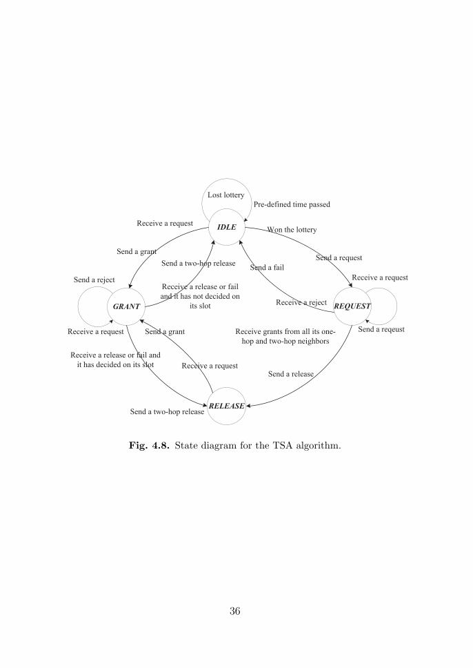
4.2.1 TSA algorithm
A TSA algorithm runs in rounds and the duration of each round is dy-
namically adjusted depending on the estimated channel access delay of
the network. Fig. 4.8 shows the state diagram for the TSA algorithm. In
the TSA algorithm, there are four states that a node have to maintain:
IDLE, REQUEST, GRANT, and RELEASE. During the IDLE state, a
initiation node, called nI , runs a lottery that has pre-defined transmis-
sion probability. If it wins the lottery, it moves to the REQUEST state
in order to broadcast a request message to its one-hop neighbors. If it
loses the lottery, it remains in the IDLE state. When a one-hop neigh-
bor node, called nN , receives a request message, if nN is in the IDLE or
RELEASE state, it changes into the GRANT state and transfers a grant
message. nN is in these states only when (1) no neighbors of nN have
sent a request message (2) nN has not sent any grant to any node so far;
or (3) nN has received a fail or release message after transferring a grant
message. When transferring a grant message, nN includes its frame map
that represents the bitwise expression of the slot allocation status in a
frame. When receiving a request message, if nN is in the REQUEST or
GRANT state, then it transfers a reject message to nI . When receiving
a reject message from any node, nI transfers a fail message to all its
one-hop neighbors and changes its state to the IDLE state. When nN
receives a fail message from nI whose request turned nN ’s current state
to the GRANT state, nN returns to the IDLE state if it has not decided
on its slot already, or to the RELEASE state if it has decided on its slot.
38
Fig. 4.9 illustrates a failed round because nN has sent a grant message to
its another one-hop neighbor before receiving the request message from
nI . If nI does not receive any grant or reject message from nN within
specific time, nI retransmits a request message to those nodes that it has
not received a grant message from. When a node receives a request mes-
sage from another node for which it has already sent a reject message,
then it retransmits the reject message to that node. As nI receives the
grant messages from its entire one-hop neighbors for the request message,
it decides on its time slot out of available time slots, which has not been
taken by its two-hop neighbors. After that, nI enters the RELEASE state
and broadcasts a release message containing information on its selected
time slot to its one-hop neighbors. Fig. 4.10 illustrates an example of
a successful round. On receiving a release message, a one-hop neighbor
of nI turns into the IDLE state if it has not decided on its slot or the
RELEASE state otherwise, and re-broadcasts that the received release
message to its one-hop neighbors. This second broadcasting message is
called two-hop release message in this dissertation. If a neighbor node
does not receive a fail or release message after transferring a grant mes-
sage to nI for some time, it retransmits the grant message. If a node
receives a grant message for which it has previously sent a fail or release
message, then it retransmits the fail or release message to that node. If
each node experiences a successful round, each node is ready to get a slot
for the interference-free communication
39

4.2.2 MSA algorithm
In the proposed MSA algorithm, an SA packet is employed for transfer-
ring the information on the allocated slot index to the next node and
following terminologies are used.
• forward/reverse path: path to the destination/source node;
• TN/RN: a transmitting node and a corresponding receiving node
in an allocated slot;
• Sindex: the slot index allocated;
• next node: a neighbor peer node to the destination node in a for-
ward path;
• MACNEXT : MAC address of a next node;
• MACSOURCE: MAC address of a source node;
• MACDESTINATION : MAC address of a destination node.
Some of the above terms are shown in Fig. 4.7.
Table 4.1 lists the size of each message field used. The field size for
an ID and an address is based on the values in [69]. If a source node is
ready for the slot allocation in a flow, then it unicasts the SA packet to
the next node on the path after operating the TSA algorithm.
Algorithm 1 shows the MSA algorithm initiated by a source node.
Further, Algorithm 2 shows the MSA algorithm when either an inter-
mediate node or a destination node receives an SA packet from node
40

Algorithm 1 MSA in a source node
1: if k = 1 then
2: p1 first runs the TSA algorithm.
3: p1 sets sindex to the slot index of the obtained slot.
4: p1 marks the obtained slot as a TN.
5: p1 transfers the SA packet with sindex to p2.
6: end if
Algorithm 2 MSA in an intermediate/a destination node
1: if 1 < k < q then
2: Based on the received sindex, pk allocates the slot(s) for both pk−1
and pk as an RN.
3: pk runs the TSA algorithm.
4: pk sets sindex to the slot index of the obtained slot.
5: pk marks the obtained slot as a TN.
6: pk transfers the SA packet with sindex to pk+1.
7: else if k = q then
8: Based on the received sindex, pq allocates the slot(s) for both pq−1
and pq as an RN.
9: pq transfers the SA completion message to the source node p1.
10: end if
pk (1 ≤ k < q, q ≥ 2) in a forward path. An intermediate node or a
destination node invokes Algorithm 2 whenever it receives an SA packet
wherein MACNEXT is equal to its MAC address. In Algorithm 2, when
an intermediate node performs the TSA algorithm to allocate the slot
41

as a TN, it is very important for the intermediate node to reserve the
right-hand side slot for comparison with the sindex within the SA packet
received, such that multihop links can be sequentially scheduled on a
path.
4.2.3 Performance analysis
4.2.3.1 Correctness of TSA
Theorem 1. The execution of TSA algorithm results in each node’s per-
forming conflict-free TDMA schedule.
Proof. The validity of the slots scheduled by the TSA algorithm can be
verified by the following three conditions.
• A node must receive grant messages from all the one-hop neighbors;
• Any nodes, which are two-hop away from each other, share at least
one common one-hop neighbor;
• A node transfers at most one grant message per round.
Based on the above conditions, in the TSA algorithm, the grant mes-
sages contain the frame map that represents the information on the slots
already taken by their one-hop neighbors. This property make sure that
a node always selects the slot that is not taken by two-hop neighbors and
any nodes within two hop neighbors can not select the same time slot.
42

4.2.3.2 Complexity analysis of TSA algorithm
Each node i in the network runs the TSA algorithm during up to ∆
rounds. One round time is set to T∆ seconds. Every node must try
the lottery at least once and at most ∆ times. In order for a node i to
finish slot selection, T∆ must be sufficiently long to (a) transfer a request
message, (b) receive grant messages from all its one hop neighbors, (c)
select the minimum time slot available and (d) transfer a release message.
Theorem 2. Assuming the round time is bounded by some constants,
the expected number of rounds for a node to acquire a slot is less than
(δ′ + 1) · e∆.
Let pi(k) be the probability that node i tries to perform the lottery
in the kth round. Since δ′ contenders of a node i can have at most ∆
lottery tries, the probability that node i acquires a slot in the tth round,
psucc(i, t), is bounded as follows:
psucc(i, t) ≥ psucc(i, 1) (4.3)
≥ pi(1)∏j∈c(i)
∆∏k=1
(1−pj(k)) (4.4)
≥ 1
δ′ + 1
∏j∈c(i)
(1− pj(k))∆, (4.5)
where δ′ denotes two-hop degree that means the maximum number of
two-hop neighbors in the network.
Because pj(∆) ≥ p(k) for 1 ≤ k ≤ ∆, equation (4.5) can be replaced
43

by
1
δ′ + 1
∏j∈c(i)
(1− pj(∆))∆. (4.6)
Next, because δ′ is two-hop degree, pj(∆) ≤ 1/(δ′ + 1). Therefore,
equation (4.6) can be given by
1
δ′ + 1
δ∏j=1
′(1− 1
δ′ + 1)∆
(4.7)
=1
δ′ + 1(1− 1
δ′ + 1)δ
′∆ (4.8)
>1
δ′ + 1e−∆. (4.9)
where (1− 1/(δ′ + 1))δ ′ > e−1.
Since the above result is independent of i and k, it gives the lower
bound on the probability that a node acquires a slot in any round. Let
M be the random number representing the number of rounds before a
node acquires a slot with the lower bound probability. M definitely has
a geometric distribution[22].
Pr(M = k) = plow(1− plow)k−1, (4.10)
where plow = 1/[(δ′ + 1) · e∆
].
From the above result, we can obtain the upper bound on the expected
number of rounds that a node takes to acquire a slot as follows:
E [M ] =1
plow= (δ′ + 1) · e∆. (4.11)
Theorem 3. Assuming that the message delay is bounded by a constant,
the expected message complexity of the TSA algorithm is O(δ′).
44

Proof. In each round, a contender can try the lottery for ∆ times. In
each try, it can be a winner and gets rejected, thus transferring O(1)
messages. Therefore, in one round, it can transfer O(∆) messages. Since
there are O(δ′) rounds on average, each process can transfer O(∆ × δ′)
messages on average.
4.2.3.3 Overhead analysis
In this section, we evaluate the overhead of the proposed MSA algorithm
in terms of the power consumed for the scheduling by all the nodes in the
network. The proposed scheme gets the map information on its one-hop
neighbors in each hop on the path before transferring the SA packet to the
next node. Considering all the possible combinations, we find that the
total power consumed for performing TSA and MSA algorithms, Ptotal,
consists of the following four components.
• PREQ: power consumed by request messages by all the nodes;
• PGRN : power consumed by grant messages by all the nodes;
• PREL: power consumed by release messages by all the nodes;
• PSA : power consumed by SA packets by all the nodes.
Assuming that all the nodes in the network are evenly distributed,
one-hop degree δ of all nodes is same. Therefore, PREQ can be calculated
by
PREQ =N∑i=1
h(i)∑j=1
lREQ · ptx + δ · lREQ · prx+ lACK · ptx + δ · lACK · prx
, (4.12)
45

where N denotes the total number of nodes; h(i), the total number of
hops necessary for the ith source node to transfer its packet to its desti-
nation node; δ, the one-hop degree in a node; lREQ, the sum of lreq and
lM+P ; lM+P , the sum of the overhead in MAC and PHY layers; and lACK ,
the length of the ACK packet. Further, ptx denotes the energy spent in
transmitting a bit over a distance of 1-meter, and prx denotes the energy
spent in receiving a bit. In case of PGRN , all one-hop neighbor nodes,
whose number is δ, respond to the request message transferred from the
initiation node nN . Therefore, PGRN can be calculated by
PGRN =N∑i=1
h(i)∑j=1
δ · (lGRN · ptx + δ · lGRN · prx)
+ δ · (lACK · ptx + δ · lACK · prx)
, (4.13)
where lGRN denotes the length of the grant message whose length is same
as the sum of lgrn and lM+P .
Similar to the calculation of PREQ, PREL can be given by
PREL =N∑i=1
h(i)∑j=1
lREL · ptx + δ · lREL · prx+ lACK · ptx + δ · lACK · prx
, (4.14)
where lREL denotes the length of the grant message whose length is same
as the sum of lrel and lM+P .
Finally, during performing the MSA algorithm in the network, the
SA packets are transferred as many as δ × h × N . Therefore, similar to
the calculation of PREQ, PSA can be calculated by
PSA =N∑i=1
h(i)∑j=1
lSA · ptx + lSA · prx · δ
+lACK · ptx + lACK · prx · δ
. (4.15)
46
time
TM
i-th frame
TS-D
delay components
primary queuing delay
(S) (D)
(i-1) th frame
packet arrival0.5TM
TM
T
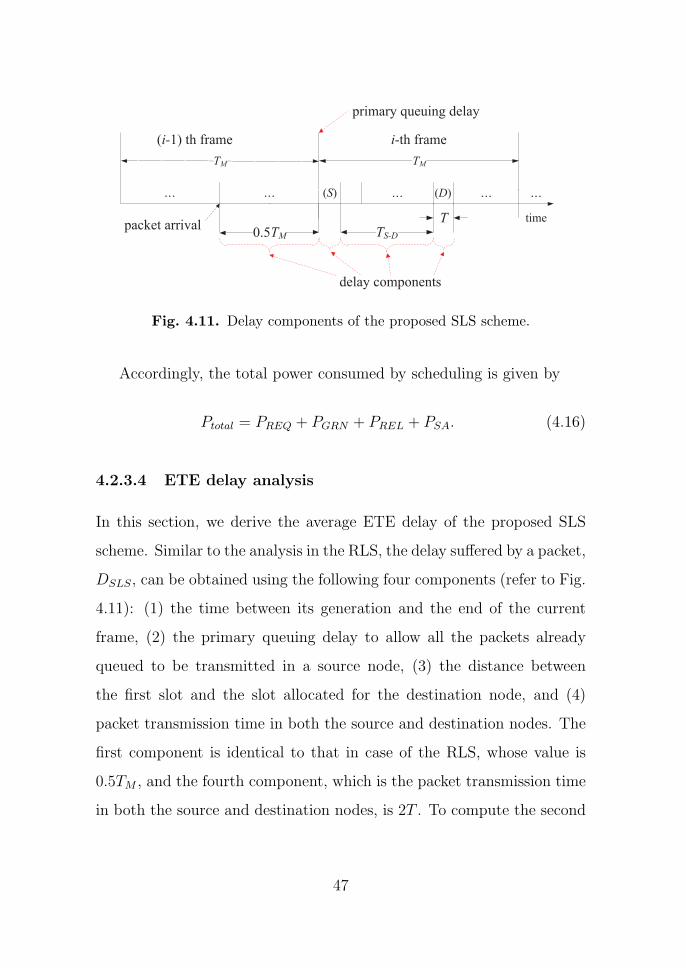
Fig. 4.11. Delay components of the proposed SLS scheme.
Accordingly, the total power consumed by scheduling is given by
Ptotal = PREQ + PGRN + PREL + PSA. (4.16)
4.2.3.4 ETE delay analysis
In this section, we derive the average ETE delay of the proposed SLS
scheme. Similar to the analysis in the RLS, the delay suffered by a packet,
DSLS, can be obtained using the following four components (refer to Fig.
4.11): (1) the time between its generation and the end of the current
frame, (2) the primary queuing delay to allow all the packets already
queued to be transmitted in a source node, (3) the distance between
the first slot and the slot allocated for the destination node, and (4)
packet transmission time in both the source and destination nodes. The
first component is identical to that in case of the RLS, whose value is
0.5TM , and the fourth component, which is the packet transmission time
in both the source and destination nodes, is 2T . To compute the second
47
component, i.e., primary queuing delay, (once the end of the current
frame is reached), we observe that the queue behaves exactly like the one
with a deterministic service time of TM . If we assume a Poisson arrival
process of λ packets/s for a user and that the number of packets that can
be stored in a queue is not bounded, then the primary queuing delay is
identical to the queuing time in an M/D/1 queuing system in which the
deterministic service time is TM . Thus, the expected primary queuing
time of a packet, Wq, is given by [70],[71]
Wq =ρ
2(1− ρ)· TM =
ρ
2(1− ρ)· LSLS · T, (4.17)
where ρ = λ · TM . If we consider a deterministic packet arrival and a
deterministic service time, then Wq is equal to zero[14]. On the other
hand, the third component, which is the distance between the first slot
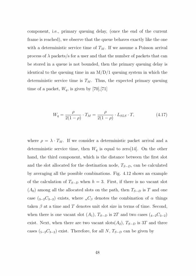
and the slot allocated for the destination node, TS−D, can be calculated
by averaging all the possible combinations. Fig. 4.12 shows an example
of the calculation of TS−D when h = 3. First, if there is no vacant slot
(A0) among all the allocated slots on the path, then TS−D is T and one
case (3−2C3−2) exists, where αCβ denotes the combination of α things
taken β at a time and T denotes unit slot size in terms of time. Second,
when there is one vacant slot (A1), TS−D is 2T and two cases (4−2C3−2)
exist. Next, when there are two vacant slots(A2), TS−D is 3T and three
cases (5−2C3−2) exist. Therefore, for all N , TS−D can be given by
48

N slots
e1A0
A1
A2
e1
e1
e1
e1
e1
e2
e2
e2
e3
e2
e2
e2
e3
e3
e3
e3
e3
AN-3
e1 e2 e3
e1 e3e2
Fig. 4.12. Example of TS−D calculation.
TS−D =
L∑j=h
j − 2
h− 2
· (j − 2)
L∑j=h
j − 2
h− 2
· T. (4.18)
Accordingly, the total ETE delay suffered by a packet, DSLS, is given
by
DSLS = 0.5TM +Wq + TS−D + 2T. (4.19)
4.2.4 Performance evaluation
For the performance evaluation, two scenarios are considered. In Scenario
#1, to observe the queuing behavior of the conventional MLS scheme us-
ing distance-2 graph coloring and the proposed SLS scheme, we simulate
49

five X by X grid networks, where X is set as 3, 4, 5, 6, and 7 when only
one packet is transferred from each source node. In the simulated net-
work, the distance between two adjacent nodes are 100 meters and the
communication range of each node is 100 meters. After each node allo-
cates slots by using distance-2 graph coloring, each source node transfers
one packet in its allocated slot. If any intermediate nodes receive packets
from the previous node on the path, they transmit the received packet in
the allocated slot. This study considers ten different seeds for this sce-
nario, and their simulation results are averaged. On the other hand, in
Scenario #2, to compare the performance of the proposed SLS scheme
with that of the MLS scheme using distance-2 graph coloring as car-
ried out in [15], this study simulates two TDMA networks with different
topologies. One is the X by X grid network, where X is set as 7. In
the grid network, the vertical and horizontal distances between two ad-
jacent nodes are 100 meters. The other is the network with 100 nodes
randomly distributed in a square area of 200 × 200 meters. In both net-
works, the communication range of each node is 30 meters. In Scenario
#2, as a consideration of primary queuing delay, we also consider both
a DPA and an NDPA having exponential distribution. These two cases
are considered for observing the behavior for both non-constant and con-
stant packet interarrival characteristics. As soon as all the source nodes
complete the proposed MSA algorithm successfully, they generate pack-
ets before transmitting them in the allocated slot. If intermediate nodes
receive packets from the previous node on the path, they transmit the
received packets in the allocated slot for each flow. For the grid network,
50

Table 4.2. Preliminary results
Grid network(N=49) Random network(N=100)
unit slot time (T ) 0.001 sec. 0.001 sec.
LMLS 21 88
LSLS 75 200
one-hop degree 3.35 7.5
two-hop degree 5.67 11.9
h 4 4.4
this study considers five different seeds. In case of random topologies,
this study considers ten different random topologies and their simulation
results are averaged. Table 4.2 summarizes some preliminary results ob-
tained from the simulation. In Table 4.2, LMLS denotes the frame length
of the MLS scheme using distance-2 graph coloring and LSLS denotes the
frame length of the proposed SLS scheme. The conventional MLS scheme
shares a common slot in a link. Therefore, the frame length of the MLS
scheme only depends on the two-hop degree. On the other hand, the pro-
posed scheme allocates different slots to each link in a flow. Therefore,
the frame length of the proposed SLS scheme is affected on the number
of nodes in the network, the average number of hops, and the number
of flows per node. The more the number of nodes, the average number
of hops, and the number of flows per node become, the bigger the frame
length.
51

Table 4.3. Parameters for overhead calculation
Parameters Value (bits)
L 400
lM+P 496
lACK 496
lreq 8
lgrn 8 + L
lrel 8
lsa 8 + 48 + 8
lREQ lM+P + lreq
lGRN lM+P + lgrn
lREL lM+P + lrel
lSA lM+P + lsa
4.2.5 Numerical and simulation results
In this section, we first discuss the results of the overhead analysis. Next,
the simulation results from Scenario #1 are discussed. Finally, the sim-
ulation results from Scenario #2 and the related analysis results are
discussed.
52

Table 4.4. MSA overhead: power consumption
49 nodes (Joules) 100 nodes (Joules)
PREQ 0.1120 1.2474
PGRN 0.1567 1.7464
PREL 0.1120 1.2474
PSA 0.0356 0.1769
Ptotal 0.4163 4.4181
Table 4.5. MSA overhead: Routing and SA time
Operations Average time (seconds)
Routing (simulation) 0.0109 (per node)
SA process (simulation) 16.8780
SA process (analysis, ∆=1) 2.2046
SA process (analysis, ∆=2) 5.9927
SA process (analysis, ∆=3) 16.2899
SA process (analysis, ∆=4) 44.2805
53

Table 4.6. Preliminary results in the MLS
# of nodes 9 16 25 36 49
LMLS 6 7 18 21 22
h 1.44 2.13 2.72 3.22 4.10
random scheduling delay 2.2 3.5 5.7 7.5 9.4
4.2.5.1 Results from overhead analysis
Table 4.3 lists the parameters used for calculating the MSA overhead. As
same in [66],[72],[73], ptx and prx are set as 0.1 nJ/bit-m2 and 50 nJ/bit,
respectively. Table 4.4 lists the energy spent by all the nodes for the
proposed MSA algorithm. Typically, a distributed network having 100
nodes needs a couple of joules of energy for scheduling[66],[72],[73]. In the
proposed MSA algorithm, all nodes exchange their frame maps for each
hop in a flow. Therefore, the energy consumed is slightly more than that
consumed in the conventional schemes. However, it is believed that these
results are within the acceptable range. Table 4.5 lists the MSA overhead
in terms of routing and SA time. According to the simulation, the time
taken to complete the SA process is approximately 16.8780 seconds. This
value is almost same as the one of the analytical result when ∆ is 3, which
means that each node needs about at most three rounds to complete the
SA process.
54

4.2.5.2 Results from Scenario #1
Table 4.6 summarizes some results from the simulation of Scenario #1,
where each source node transfers only one packet in the first frame.
In Table 4.6, LMLS denotes the number of slots allocated by distance-
2 graph coloring and random scheduling delay denotes the number of
frames elapsed for all the destination nodes to receive one packet from
each source node. In the conventional MLS schemes where one common
slot is allocated to multiple flows in a link, the factors that may influence
random scheduling delay are primary and secondary queuing delays. In
this scenario, no primary queuing delay occurs because each node gen-
erates only one packet. Intuitively, it is said that if the number of hops
from a source node to a destination is h, the ETE delay in terms of frames
is h. However, as shown in Table 4.6, each network (when X is 3, 4, 5,
6, and 7) needs 2.2, 3.5, 5.7, 7.5, and 9.4 frames on an average when h
is 1.44, 2.13, 2.72, 3.22, and 4.10, respectively. Thus, the increase of the
random scheduling delay in Scenario #1 is all caused by the secondary
queuing delay. Accordingly, in multihop environments, the MLS causes
ETE delay to be increased because of secondary queueing delay although
there is no primary queueing delay.
55

0 0.1 0.2 0.3 0.4 0.5 0.6 0.7 0.8 0.9 1.0
500
1,000
1,500
2,000
500
1,000
1,500
2,000
ET
E d
elay
( #
of
slo
ts)
Proposed SLS (-2 dBm)
Proposed SLS (-1 dBm)
Proposed SLS (0 dBm)
Proposed SLS (No error)
Conventional MLS (-2 dBm)
Conventional MLS (-1 dBm)
Conventional MLS (0 dBm)
Conventional MLS (No error)
Fig. 4.13. ETE delay with different traffic load and TX power: DPA.
56

0 0.1 0.2 0.3 0.4 0.5 0.6 0.7 0.8 0.9 1.0
500
1,000
1,500
2,000
500
1,000
1,500
2,000
ET
E d
elay
(#
of
slo
ts)
Proposed SLS (-2 dBm)
Proposed SLS (-1 dBm)
Proposed SLS (0 dBm)
Proposed SLS (No error)
Conventional MLS (-2 dBm)
Conventional MLS (-1 dBm)
Conventional MLS (0 dBm)
Conventional MLS (No error)
Fig. 4.14. ETE delay with different traffic load and TX power: NDPA.
57
4.2.5.3 Results from Scenario #2
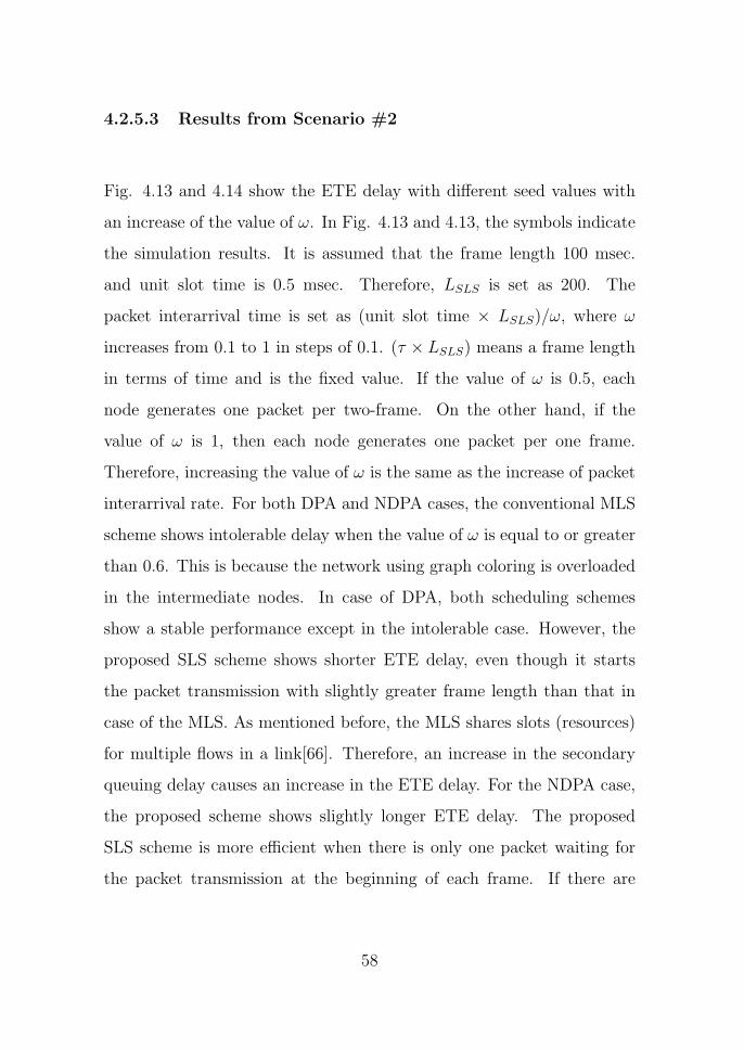
Fig. 4.13 and 4.14 show the ETE delay with different seed values with
an increase of the value of ω. In Fig. 4.13 and 4.13, the symbols indicate
the simulation results. It is assumed that the frame length 100 msec.
and unit slot time is 0.5 msec. Therefore, LSLS is set as 200. The
packet interarrival time is set as (unit slot time × LSLS)/ω, where ω
increases from 0.1 to 1 in steps of 0.1. (τ × LSLS) means a frame length
in terms of time and is the fixed value. If the value of ω is 0.5, each
node generates one packet per two-frame. On the other hand, if the
value of ω is 1, then each node generates one packet per one frame.
Therefore, increasing the value of ω is the same as the increase of packet
interarrival rate. For both DPA and NDPA cases, the conventional MLS
scheme shows intolerable delay when the value of ω is equal to or greater
than 0.6. This is because the network using graph coloring is overloaded
in the intermediate nodes. In case of DPA, both scheduling schemes
show a stable performance except in the intolerable case. However, the
proposed SLS scheme shows shorter ETE delay, even though it starts
the packet transmission with slightly greater frame length than that in
case of the MLS. As mentioned before, the MLS shares slots (resources)
for multiple flows in a link[66]. Therefore, an increase in the secondary
queuing delay causes an increase in the ETE delay. For the NDPA case,
the proposed scheme shows slightly longer ETE delay. The proposed
SLS scheme is more efficient when there is only one packet waiting for
the packet transmission at the beginning of each frame. If there are
58

more than two packets at the beginning of each frame, then all packets
but one packet to be transferred in the current frame experience a long
delay because of long frame length. When considering the NDPA case
in the source node, each source node has the chance to see more than
two packets; i.e., the primary queuing delay may occur. Therefore, the
proposed SLS scheme shows a slightly lower delay performance for the
NDPA case. However, the proposed scheme is more tolerable for a high
packet interarrival rate than the MLS.
4.3 Summary
In this chapter, a sequential link scheduling scheme called SLS was pro-
posed to reduce ETE delay in multihop WMNs. The proposed scheme
allocates a different slot to each flow in a link to eliminate secondary
queueing delay. Additionally, all slots are allocated with the allocation
order on a path considered in order to eliminate random scheduling de-
lay, ultimately reducing ETE delay in multihop WMNs. We derived the
ETE delay of the proposed scheme and validated it through a simula-
tion. Finally, we compared the performance of the proposed scheme with
that of the conventional the MLS scheme that employs distance-2 graph
coloring. The important contributions of this study are as follows:
• Analysis of the delay effect caused by an allocation order of the
TDMA slots was performed;
• Channel locking algorithm called TSA for interference-free commu-
59
nication was proposed;
• Complexity analysis of the TSA algorithm was performed;
• Fully distributed method to sequentially allocate slots on a path,
called MSA, was proposed;
• Delay analysis of the proposed scheme and its simulation were per-
formed.
According to the analysis and simulation results, for deterministic
packet arrival, the proposed scheme works well irrespective of the packet
interarrival rate and outperforms the conventional MLS. However, in
case of non-deterministic packet arrival, the ETE delay of the proposed
SLS scheme is slightly longer than that of the conventional MLS because
the probability that each node has more than two packets increases at
the beginning of the frame. However, the proposed SLS scheme is more
tolerant for a high packet interarrival rate.
60

5
Sequential Scheduling jointly
combined with NC in
TDMA-based WMNs
In the fields of TDMA-based WMNs, several NC schemes have been
proposed[34],[74]. They have focused on the improvement of network
throughput efficiency that is the original objective of NC. However, al-
though they can get NC gain, ETE delay may be varied according to the
allocation order of slots in TDMA-based WMNs. Therefore, this disserta-
tion proposes two joint scheduling and NC schemes to reduce ETE delay
with NC gain guaranteed, which performs XOR-based NC operation, in
distributed TDMA-based WMNs.
61
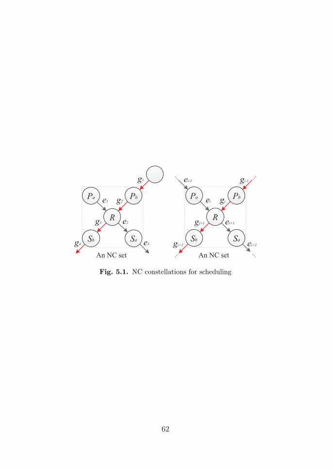
ei-1
ei
ei+1
gj
ei+2
gj-1
gj+1
gj+2
e1
e2
e3
g2
g3
g4
g1
eee
An NC set An NC set
Sa
R
Pa Pb
SbSa
R
Pa Pb
Sb
Fig. 5.1. NC constellations for scheduling
62

e1g1 g2 g3 g4
e2
1 2 3 4 5 6 7 8 9 10 11 12 13
Fig. 5.2. Delay effect in an RLS with NC: case 1
e2e1g4 g2 g3 g1
1 2 3 4 5 6 7 8 9 10 11 12 13
Fig. 5.3. Delay effect in an RLS with NC: case 2
e3 g3g1e1 e2 g2 g4
1 2 3 4 5 6 7 8 9 10 11 12 13
Fig. 5.4. Example of an SLS with NC
63

5.1 Motivation
Consider an NC set as shown in Fig. 5.1(right). An reference NC flow fr
in an NC set is referred to as the first flow that has finished a scheduling
procedure and a non-reference NC flow fn is referred to as the last flow
that has finished a scheduling procedure out of two NC flows. From
now onward, in each figure, we use link indexes e and g for fr and fn,
respectively. We also define s(ei) and s(gj) as slot indexes of the links
ei and gj, respectively, where i (≥ 1) and j (≥ 1) denote link indexes.
First, we consider an RLS scheme used in an environment where there
is no central node or base station in the network; i.e., in a distributed
environment. Because there is no central node, link g1 and g4 not related
to the NC operation may be allocated slots as shown in Fig. 5.2 or Fig.
5.3. It is assumed that the slots for NC flows are sequentially scheduled.
In this case, the sixth slot becomes the common broadcasting slot. Let
random scheduling delay be the number of frames required to transfer
a packet from a source to a destination. In case of Fig. 5.2, random
scheduling delay is one. However, in case of Fig. 5.3, random scheduling
delay is two. Random scheduling delay varies according to both the
slot allocation order within a frame and the number of hops. Therefore,
this random scheduling delay must be considered to reduce ETE delay
when NC is performed in distributed TDMA-based WMNs. On the other
hand, consider conventional SLS schemes[15],[75] that have considered
the allocation order of slots within a frame. They can guarantee the
sequentiality of slots only for its own flow on a path, where, if defined
64

in different angle, ‘sequentiality’ means the slot allocation satisfying the
condition s(ei) < s(ei+1) for the links ei (1 ≤ i ≤ h) in a flow. If
the slots scheduled in a flow satisfy with the sequentiality, the multihop
transmission of a packet from a source node to a destination node is
possible within one frame. However, if considering NC for which two
flows are mixed, this sequentiality may be broken. For example, Fig. 5.4
shows an example where the sequentiality is broken in the conventional
sequential link scheduling schemes. Assume that, in the NC set of Fig.
5.1(left), the links e1 and g2 are the ones from previous nodes and the links
e2 and g3 are the ones to the next nodes. If we set a common broadcasting
slot as s(e2), then the links of fr are arranged in the sequence of s(e1),
s(e2), and s(e3), and the links of fn are arranged in the sequence of s(g3),
s(g1), s(g2), and s(g4). Therefore, the links of fn do not satisfy with the
sequentiality. On the other hand, if we set a common broadcasting slot
as s(g3), then the links of fr are arranged in the sequence of s(e1), s(e3),
and s(e2), and the links of fn are arranged in the sequence of s(g1),
s(g2), s(g3), and s(g4). In this case, the links of fr do not satisfy with
the sequentiality. Therefore, in order that NC operation is performed
with the sequentiality satisfied, the slot indexes of the links ei and gj of
two predecessor nodes must precede the slot indexes of the links ei+1 and
gj+1 of two successor nodes (refer to Fig. 5.1(right)).
65

5.2 Proposed Section-based Scheme
The proposed section-based sequential scheduling scheme with NC, which
is flow-based one, employs a new concept, ‘section’, so that the slots
scheduled on a path are sequentially arranged within a frame even when
NC is used. It is assumed that all the nodes know H that denotes the
highest value of hop distance in the network. We define h(i) as hop
information to the destination, which a source node i obtains after the
completion of routing process. Before performing the proposed section-
based scheme, each source node broadcasts its own h(i). When a node
hears h(i), if the received hop value is higher than the one it currently
knows, it rebroadcasts the new value. After some predetermined dissem-
ination time, all the nodes obtain the highest hop value H. By using
this hop information, the network divides a frame to H sections. We
also define x(ei) and x(gj) as the section indexes of the links ei and gj,
respectively. We first describe the proposed section-based scheme when
not using NC operation. In the proposed section-based scheme, all nodes
allocate slots by using section and hop information.
66

e1 e2g1 g2 g3 g4
Fig. 5.5. Example of the slot allocation when h(i)= 2 and 4 for four
sections
e1 e2 e3 e4g1 g2 g3
Fig. 5.6. Example of the slot allocation when h(i)= 4 and 3 for four
sections
67
During the routing process, each node manages the routing tables
(forward and reverse tables). Based on both these two tables and the
criteria for NC sets explained in section 2.2, prior to performing the
proposed scheme, each node finds NC sets where NC operation is possible.
Although the routing table is altered because of the change of the cost
metric, nodes in the network do not perform a new SA process. That
is, once slots are determined by the SA process, the network exploits the
slots for the lifetime of flows.
Fig. 5.5 and 5.6 show examples of the slot allocation in the proposed
section-based scheme when H is 4, and h(i) is either 2 and 4 or 4 and 3.
Now, we describe the scheduling procedure when the proposed section-
based scheme is jointly combined with NC operation. According to the
result in [76], if considering energy requirements, it is reported that less
than 1% of coding operations are related to the combination of more
than three packets. Therefore, in this dissertation, it is assumed that an
NC coordinator that performs XOR-based NC operation manages only
two flows. As mentioned before, if the allocation order in each link is not
considered, random scheduling delay may be increased, thereby increas-
ing ETE delay. Therefore, when performing a slot allocation procedure,
the slot indexes scheduled for the links ei and gj of two predecessor nodes
must precede the slot indexes scheduled for the links ei+1 and gj+1 of two
successor nodes (refer to Fig. 5.1(right)). If considering all possible com-
binations of the slot allocation in an NC set, there exist four conditions
as follows:
• x(ei) = x(gj);
68
• x(ei) = x(gj) + 1;
• x(ei) = x(gj) - 1;
• x(ei) < x(gj) - 1 or x(ei) > x(gj) + 1 where j ̸= 1.
69

ei-1 gj-1 ei gj ei+1 gj+1 ei+2 gj+2
Fig. 5.7. NC condition 1: x(ei) = x(gj)
ei-1gj-1 eigj ei+1gj+1 ei+2gj+2
Fig. 5.8. NC condition 2: x(ei) = x(gj) + 1
ei-1 gj-1ei gjei+1 gj+1ei+2 gj+2
Fig. 5.9. NC condition 3: x(ei) = x(gj) - 1
ei-1 gj-1ei gjei+1 gj+1ei+2
Fig. 5.10. NC condition 4: x(ei) < x(gj) - 1 or x(ei) > x(gj) + 1
70

Fig. 5.7 through 5.10 illustrate four NC conditions mentioned above.
The first and second conditions can guarantee the sequentiality of the
slots on a path because the slot indexes of the links ei and gj always
precede the slot indexes of the links ei+1 and gj+1. Therefore, NC coor-
dinator R sets either one out of the slots for the links ei+1 and gj+1 as a
common broadcasting slot. In the third case, the slot index for the link
ei+1 precedes the slot index for the link gj. In this case, by swapping the
slot indexes for ei+1 and gj, we can guarantee the sequentiality. How-
ever, this case needs an overhead that the NC coordinator R exchanges
another control packet with Pb. In the last case (Fig. 5.10), the slot
index for the link ei+1 precedes the slot index for the link gj. In this
case, the NC coordinator R has two options. One is to set the slot sched-
uled for gj+1 as a common broadcasting slot, resulting in the link indexes
with a sequence of ei−1, ei, ei+2, and ei+1. Therefore, the sequentiality
is broken. The other is to select the slot scheduled for ei+1 as a common
broadcasting slot, resulting in the link indexes with a sequence of gj+1,
gj−1, and gj. This case also does not satisfy with the sequentiality on
a path. The NC coordinator R of the proposed section-based scheme
can decide on whether or not performing an NC operation for the fourth
case. The decision may be different depending on the QoS requirements
of applications. Algorithm 3 and 4 show the SA process of the proposed
section-based scheme.
71

Algorithm 3 Slot allocation in a source node
1: if k = 1 then
2: p1 first runs the TSA algorithm.
3: p1 sets sindex to the slot index of the obtained slot.
4: p1 marks the obtained slot as a TN.
5: p1 transfers the SA packet with sindex to p2.
6: end if
72

Algorithm 4 Slot allocation in an intermediate/a destination node
1: if 1 < k < q then
2: if (pk = NC coordinator)&&(current flow = fn) then
3: if x(ek) = x(gk) then
4: pk invokes Algorithm 5.
5: else if x(ek) = x(gk) + 1 then
6: pk invokes Algorithm 6.
7: else if x(ek) = x(gk) - 1 then
8: pk invokes Algorithm 7.
9: else
10: pk invokes Algorithm 8.
11: end if
12: else
13: Based on received sindex, pk allocates the slot for both pk−1 and
pk in the section x(gk−1) as an RN.
14: Then, pk obtains the frame map of its one-hop neighbors.
15: pk allocates the commonly available slot for both pk and pk+1 in
the section x(gk) as a TN.
16: pk transfers an SA packet with sindex to pk+1.
17: end if
18: else if k = q then
19: Based on received sindex, pq allocates the slot for both pq−1 and pq
as an RN.
20: pq transfers an SA completion message to the source node p1.
21: end if
73

Algorithm 5 Process for 1st NC condition
1: Based on received sindex, pk allocates the slot for both pk−1 and pk in
the section x(gk−1) as an RN.
2: pk gets sindex for the link ek+1 and allocates the common broadcasting
slot for NC as a TN.
3: pk transfers an SA packet with that sindex to pk+1.
Algorithm 6 Process for 2nd NC condition
1: Based on received sindex, pk allocates the slot for both pk−1 and pk in
the section x(gk−1) as an RN.
2: pk gets sindex for the link ek+1 and allocates the common broadcasting
slot for NC as a TN.
3: pk transfers an SA packet with that sindex to pk+1.
74

Algorithm 7 Process for 3rd NC condition
1: pk swaps the slot index for the link ek+1 for the slot index for the link
gk.
2: pk informs pk−1 of the information on the new slot index for gk.
3: pk sets sindex to the swapped new slot index for the link ek+1.
4: pk transfers an SA packet with sindex to pk+1.
Algorithm 8 Process for 4th NC condition
1: Based on received sindex, pk allocates the slot for both pk−1 and pk in
the section x(gk−1) as an RN.
2: Then, pk obtains the frame map of its one-hop neighbors.
3: pk allocates the commonly available slot for both pk and pk+1 in the
section x(gk) as a TN.
4: pk transfers an SA packet with sindex to pk+1.
75

5.2.1 Performance analysis
5.2.1.1 Power consumption analysis
For calculating the power consumed by the proposed section-based scheme,
two additional components should be considered as compared with the
proposed SLS scheme. In the 3th NC condition of the proposed section-
based scheme, NC coordinatorR informs the node pk−1 of the information
on the new slot index for gk. This additional transmission to the node
pk−1 is the first consideration. According to the simulation, the ratio of
such cases to total NC points is less than approximately 10%. Therefore,
this dissertation ignores this consideration because the power consumed
by these transmissions is very small compared to the total power con-
sumed. On the other hand, the proposed SLS scheme exchanges the
frame map whose length is equal to the one of the frame length. How-
ever, the proposed section-based scheme exchanges the frame map whose
length is (⌈lgrn/H⌉ + lM+P ). Therefore, we can obtain the total power
consumed by the proposed section-based scheme by replacing lGRN to
(⌈lgrn/H⌉ + lM+P ) in equation (3.13). Then, the total power consumed
by the transmission of the grant messages is calculated by
PGRN(SEC) =N∑i=1
h(i)∑j=1
δ ·
(⌈lgrn/H⌉+ lM+P ) · ptx+δ · (⌈lgrn/H⌉+ lM+P ) · prx
+ δ · (lACK · ptx + δ · lACK · prx)
, (5.1)
where ⌈∗⌉denotes a smallest integer more than or equal to ∗. Accordingly,
the total power consumed by the proposed section-based scheme is given
76

by
Ptotal(SEC) = PREQ + PGRN(SEC) + PREL + PSA. (5.2)
5.2.1.2 ETE delay analysis
In this section, the ETE delay analysis of the proposed section-based
scheduling scheme without NC is performed. In the proposed scheme, all
nodes allocate slots by using section and hop information. First of all,
assume that the hop distance h(i) of source node i is evenly distributed.
For example, the number of source nodes having the hop distance of
one, two, ..., H is all same where H denotes the maximum number of
hops in the network. Thus, all N nodes in the network try to allocate
slots in the section x(1). In the section x(2), (N − N/H) nodes try to
allocate slots and ,in the last section x(H), N/H nodes try to allocate
slots. Accordingly, given L slots, the number of slots necessary in ith
section, Li, can be calculated by
Li =
N−(i−1)NH
H∑j=1
{N−(j−1)NH}
· L
, i ̸= H
L−H−1∑k=1
N−(k−1)NH
H∑j=1
{N−(j−1)NH}
· L
, i = H
(5.3)
where ⌊∗⌋ means the integer less than or equal to *. Also, the ETE delay
a packet experiences in the section x(i) is composed of three components:
(1) time between the start of the frame and the end of (i−1)th section, (2)
time between the start of ith section and the slot scheduled for the desti-
nation in ith section, and (3) the transmission time at the destination. If
77

Algorithm 9 Slot allocation in a source node
1: if k = 1 then
2: p1 first runs the TSA algorithm.
3: p1 sets sindex to the slot index of the obtained slot.
4: p1 marks the obtained slot as a TN.
5: p1 transfers the SA packet with sindex to p2.
6: end if
considering the above components, the ETE delay a packet experiences
in the section x(i) is given by
DSEC (i) =
(i−1∑j=1
Lj
)· T +
Lj
2· T + T (5.4)
=
{(i−1∑j=1
Lj
)+Lj
2+ 1
}· T, (5.5)
where T denotes unit slot time.
Finally, the average ETE delay is given by
DSEC =
H∑k=1
DSEC(k)
H. (5.6)
From equation (5.6), it can be seen that the average ETE delay is the
function of the frame size L. Therefore, the average ETE delay of the
proposed scheme is increased as the frame size is increased.
5.3 Proposed DARR-based Scheme
Algorithm 9 and 10 show the MSA algorithm of the proposed DARR-
based scheme. In Algorithm 9 and 10, sindex denotes an allocated slot
78

Algorithm 10 Slot allocation in an intermediate/a destination node
1: if 1 < k < q then
2: if (pk = NC coordinator)&&(current flow = fn) then
3: Based on received sindex, pk allocates the slot(s) for both pk−1
and pk as an RN.
4: pk runs the TSA algorithm.
5: pk sets sindex to the slot index of the obtained slot.
6: pk marks the obtained slot as a TN.
7: pk transfers an SA packet with sindex twice to two pk+1 nodes of
fr and fn.
8: else
9: Based on received sindex, pk allocates the slot(s) for both pk−1
and pk as an RN.
10: pk runs the TSA algorithm.
11: pk sets sindex to the slot index of the obtained slot.
12: pk marks the obtained slot as a TN.
13: pk transfers an SA packet with sindex to pk+1.
14: end if
15: else if k = q then
16: Based on received sindex, pq allocates the slot(s) for both pq−1 and
pq as an RN.
17: pq transfers an SA completion message to the source node p1.
18: end if
79
index in a frame; TN and RN mean a transmitting node and a cor-
responding receiving node in an allocated slot, respectively; and frame
map represents the bit-wise expression of slot allocation status in a frame.
The basic idea of the proposed DARR-based scheme is that, when the
MSA algorithm has been initiated from fn, an NC coordinator not only
transfers an SA packet to the next node of fn but also again transfers
another SA packet to the next node of fr. Thus, from the links ei+1 to
eh of fr, additional slots are allocated; i.e., existing slots that have been
used and newly allocated slots for fr. At this time, the NC coordinator
releases the existing slots and, in the next frame, uses the newly allo-
cated slots for the sequentiality. The released slots may be used for other
flows. The extra transmissions for the slot release are an overhead of the
proposed DARR-based scheme. However, it is shown that they are not
big burden in the network. If considering the time difference between the
slot allocations of fr and fn, there exist the following three cases.
• Case 1: before allocating the slot for link ei+1, when NC coordinator
R receives the SA packet that includes the SA information for gj
in the current frame;
• Case 2: after allocating the slot for ei+1, when NC coordinator R
receives the SA packet that includes the SA information for gj in
the current frame;
• Case 3: after the slot allocation for fr has been already completed
in a frame, when NC coordinator R receives the SA packet that
includes the SA information for gj in a different frame.
80

g1g2
g3
e 2g4
e 3e 1
time
123456789101112123456789101112
g1g2
g3
e 2g4
e 3e 1
...
commonbroadcastingslots
g1g2
g3
e 2g4
e 3e 1
123456789101112
(a)ExampleofCase1
time
123456789101112
e 1g1
e 2e 3
e 1g1g2
g3
e 2
g4
e 3e 3
g3
g2
g1
e 2...
e 1
releasedslots
g4
commonbroadcastingslots
123456789101112123456789101112
g2
g3g4e 3
e 2
releasedslots
(b)ExampleofCase2
e 1e 2e 3
e 1e 2e 3
g1g2
g3
e 2
g4
e 3
1
time
e 3g3
g2
g1
...
e 2...
e 1
releasedslots
g4
commonbroadcastingslots
23456789101112
123456789101112123456789101112
(c)ExampleofCase3
Fig. 5.11. Examples of the proposed DARR-based scheme.
81
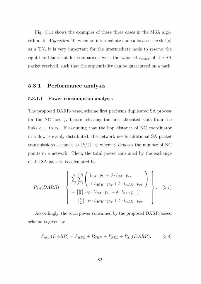
Fig. 5.11 shows the examples of these three cases in the MSA algo-
rithm. In Algorithm 10, when an intermediate node allocates the slot(s)
as a TN, it is very important for the intermediate node to reserve the
right-hand side slot for comparison with the value of sindex of the SA
packet received, such that the sequentiality can be guaranteed on a path.
5.3.1 Performance analysis
5.3.1.1 Power consumption analysis
The proposed DARR-based scheme first performs duplicated SA process
for the NC flow fr before releasing the first allocated slots from the
links ei+1 to eh. If assuming that the hop distance of NC coordinator
in a flow is evenly distributed, the network needs additional SA packet
transmissions as much as ⌈h/2⌉ · ψ where ψ denotes the number of NC
points in a network. Then, the total power consumed by the exchange
of the SA packets is calculated by
PSA(DARR) =
N∑i=1
h(i)∑j=1
lSA · ptx + δ · lSA · prx+ lACK · ptx + δ · lACK · prx
+⌈h2
⌉· ψ · (lSA · ptx + δ · lSA · prx)
+⌈h2
⌉· ψ · lACK · ptx + δ · lACK · prx
. (5.7)
Accordingly, the total power consumed by the proposed DARR-based
scheme is given by
Ptotal(DARR) = PREQ + PGRN + PREL + PSA(DARR). (5.8)
82

5.4 How to Cope with Asymmetric Flow
Conditions
Consider an asymmetric condition where the packet arrival rates of two
flows are different as shown in Fig. 5.12. If there are two packets from fr
and fn before the 5th slot (e.g., Case 1), then R performs the baseline NC
operation. However, if there is one packet from fr because of asymmetric
flow conditions (e.g., Case 2), then R has two options. First, R may
wait for the packet from fn (i.e., packet y2 in Fig. 2) to increase the
coding opportunity. Second, R may immediately transfer (i.e., unicast)
that packet for delay efficiency. Intuitively thinking, the first case causes
the ETE delay to increase. The fundamental purpose of this study is
to reduce ETE delay regardless of whether or not NC is applied to the
scheduling. Therefore, this case is not a concern of this paper. In the
second case, node Sb has the packet that is overheard from Pa. However,
because R has unicasted the packet x1 to Sa, the packet queued in Sb is
actually useless. In this case, Sb can not determine whether this packet
should be considered (or queued) for a next NC operation because node
Sb does not grasp of this situation because of unicast transmission from
R to Sa.
83

x1 y1 z1
1 2 3 4 5 6 7 8
P1
R
P2
S2 S1
x1 y1
x3x2
y2
Packet arrival sequenceCase 1
Case 2
Case 3
y1x1
z1
t1
reference NC flow, fr
non-reference NC flow, fn
Fig. 5.12. Example network where an asymmetric flow condition occurs.
84
The simple solution is to transfer another control packet to Sb in
order to delete that useless packet. However, in TDMA-based WMNs,
additional resources (or slots) for this transferring should be a priory
allocated[34], resulting in increasing the overhead per NC set per frame.
On the other hand, additional information on an NC set may be in-
cluded within a packet. It has been known that this overhead size is
approximately 5% of a packet size[35]. These two solutions mentioned
need extra slot allocation or additional control messages. Therefore, this
study proposes to employ a timer called dtimer to eliminate the useless
packet overhead at the successor node. That is, any successor node re-
lated to NC operation sets dtimer to 0 at the beginning of each frame. If
it does not receive the encoded packet from its NC coordinator within t1,
it eliminates the overhead packet queued for NC operation. t1 denotes
time between the start of the each frame and the slot scheduled for the
broadcasting slot as shown in Fig. 5.12. By making use of the timer,
the network can cope with asymmetric flow condition without additional
control messages or bandwidth waste.
5.5 Performance Evaluation
We have simulated a grid network with 49 nodes. The vertical and hor-
izontal distances between two adjacent nodes are 100-meter, and the
communication range of each node is set as 100-meters. During the sim-
ulation, each node creates one flow the realtime applications. As soon as
all source nodes complete MSA algorithm, they generate one packet per
85

TM before transmitting them in the allocated slot. Table 5.1 presents
the lists and brief explanations of the scheduling schemes that have been
considered for the performance comparison in this dissertation.
86
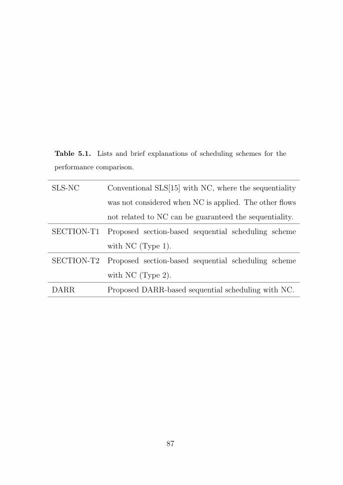
Table 5.1. Lists and brief explanations of scheduling schemes for the
performance comparison.
SLS-NC Conventional SLS[15] with NC, where the sequentiality
was not considered when NC is applied. The other flows
not related to NC can be guaranteed the sequentiality.
SECTION-T1 Proposed section-based sequential scheduling scheme
with NC (Type 1).
SECTION-T2 Proposed section-based sequential scheduling scheme
with NC (Type 2).
DARR Proposed DARR-based sequential scheduling with NC.
87

As performance metrics, we consider average ETE delay and average
coding gain. The average ETE delay means the time taken for each
source node to transfer a packet to a destination. And, the coding gain
is defined by
coding gain =h · ηtotal ·N
h · ηtotal ·N − ηNC
, (5.9)
where ηtotal denotes the total number of transferred packets per node; N
denotes the total number of nodes in the network; and ηNC denotes the
number of the transmissions reduced by NC.
88

Table 5.2. Parameters and preliminary results
Communication range (meters) 100
Number of nodes 100
Frame size in terms of slots 200
Frame size in terms of time 100 ms
Unit slot time 0.5 ms
h 4.1
H 13
Average one-hop degree 4
Average two-hop degree 10
Number of NC points 54
# of NC points not meeting 4-th NC condition 35
89
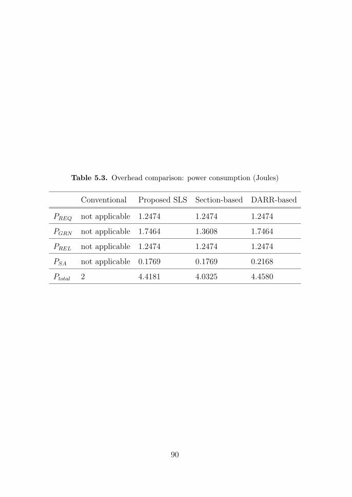
Table 5.3. Overhead comparison: power consumption (Joules)
Conventional Proposed SLS Section-based DARR-based
PREQ not applicable 1.2474 1.2474 1.2474
PGRN not applicable 1.7464 1.3608 1.7464
PREL not applicable 1.2474 1.2474 1.2474
PSA not applicable 0.1769 0.1769 0.2168
Ptotal 2 4.4181 4.0325 4.4580
90

Table 5.4. Average coding gain in the network
Lists Average coding gain
Conventional SLS-NC 1.11
SECTION-T1 1.04
SECTION-T2 1.11
DARR-based 1.11
5.6 Numerical and Simulation Results
Fig. 5.13, 5.14, 5.15, and 5.16 show the ETE delay of the conventional
and the proposed schemes with an increase in the value of ω, where
packets arrive deterministically. The packet interarrival time is set as
(unit slot time × 0.001/ω), where ω increases from 0.1 to 1 in steps of
0.1. If the value of ω is 0.5, each node generates one packet per two-frame.
On the other hand, if the value of ω is 1, then each node generates one
packet per one frame. Therefore, increasing the value of ω is the same
as the increase of packet interarrival rate. When there is no error in
wireless channel, all schemes show the stable performance regardless of
the increase in the value of ω. This is because each node generates
at most one-packet arrival per frame, resulting in no primary queuing
delay in the network. However, as TX power is decreased (0 → -1 → -2
dBm), ETE delay is increased. Especially, in the high traffic load (e.g.
when ω ≥ 0.9), the ETE delay is sharply increased. This is because the
packets experience large delay owing to the packet retransmission caused
91

by wireless channel errors, not the primary queuing delay. Meanwhile, in
the conventional SLS-NC, half of NC flows experience extra delay whose
value is TM as mentioned in section 5.1. Therefore, the conventional
SLS-NC scheme experiences the lowest delay performance. In Fig. 5.13,
5.14, 5.15, and 5.16, SECTION-T1 and SECTION-T2 denote the ETE
delay of the proposed section-based schemes with Type 1 and Type 2,
respectively. As mention in Table 5.1, ‘T1’ means one case where the
NC coordinator performs the NC operation for the fourth NC condition
and ‘T2’ (or Type 2) means the other case where the NC coordinator
does not perform the NC operation for the fourth NC condition. In
SECTION-T2, the network loses the NC gain as almost much as the
number of NC points satisfying the fourth NC condition because the NC
coordinator does not perform NC operation for the fourth NC condition.
However, the average ETE delay is smaller than that of SECTION-T1
because the sequentiality can be guaranteed. In case of SECTION-T1,
the NC coordinator does perform the NC operation for the fourth NC
condition at the cost of extra delay. Therefore, it experiences higher
delay than SECTION-T2. However, it can get the whole NC gain at the
cost of the small increase in ETE delay. Different from the conventional
SLS-NC and proposed SECTION-T1 and SECTION-T2, the proposed
DARR-based scheme can guarantee the sequentiality while the network
gets the whole NC gain. Therefore, the slots can be saved as much as
the number of the NC points, resulting in the decrease in the ETE delay
compared to SECTION-T2. On the other hand, SECTION-T2 partially
gives up NC gain for the delay efficiency. Therefore, the number of NC
92

points participated in the NC operation is decreased. As a result, DARR-
based scheme shows better delay performance than SECTION-T2. Fig.
5.17, 5.18, 5.19, and 5.20 show the ETE delay of the conventional and
the proposed schemes with an increase of the value of ω, where packets
arrive exponentially (non-deterministically). In case of non-deterministic
packet arrival, each node experiences the primary queuing delay. Each
node also experiences additional delay owing to the packet retransmission
caused by wireless channel errors. Therefore, even in the low traffic load,
each packet goes through relatively high ETE delay compared with the
deterministic packet arrival.
Table.5.4 shows the average coding gain of all the schemes used for the
performance comparison. First of all, the conventional SLS scheme does
not perform the NC operation. Therefore, there is no coding gain on it.
Meanwhile, because SECTION-T1 does not perform the NC operation
for the fourth NC condition, the average coding gain is lower than that
of other schemes. Except for SECTION-T1, all the schemes have the
same coding gain because they all performs the NC operation for all NC
points.
93

0 0.1 0.2 0.3 0.4 0.5 0.6 0.7 0.8 0.9 1.0100
120
140
160
180
200
100
120
140
160
180
200
ET
E d
elay
(#
of
slo
ts)
Conventional SLS with NC
Proposed SECTION-T1
Proposed SECTION-T2
Proposed DARR
Fig. 5.13. ETE delay in DPA case: No errors.
94

0 0.1 0.2 0.3 0.4 0.5 0.6 0.7 0.8 0.9 1.0
150
200
250
300
350
ET
E d
elay
(#
of
slo
ts)
Conventional SLS with NC
Proposed SECTION-T1
Proposed SECTION-T2
Proposed DARR
Fig. 5.14. ETE delay in DPA case: 0 dBm of TX power.
95

0 0.1 0.2 0.3 0.4 0.5 0.6 0.7 0.8 0.9 1.0
200
300
400
500
600
ET
E d
elay
(#
of
slo
ts)
Conventional SLS with NC
Proposed SECTION-T1
Proposed SECTION-T2
Proposed DARR
Fig. 5.15. ETE delay in DPA case: -1 dBm of TX power.
96
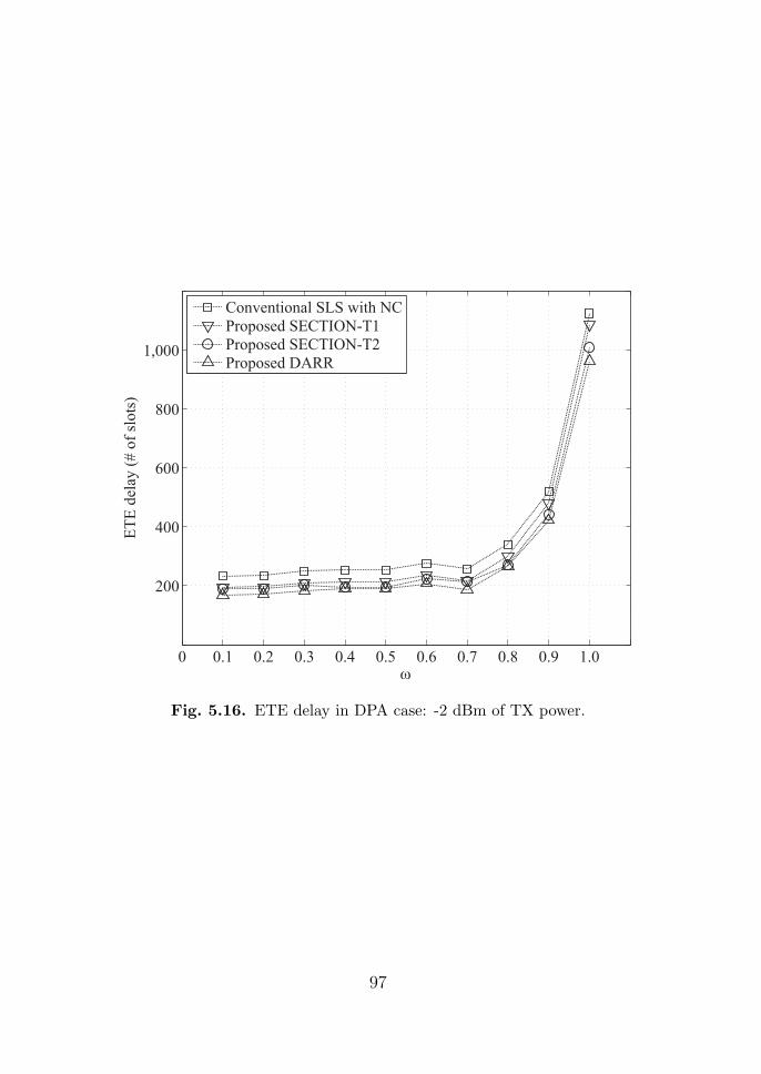
0 0.1 0.2 0.3 0.4 0.5 0.6 0.7 0.8 0.9 1.0
200
400
600
800
1,000
ET
E d
elay
(#
of
slo
ts)
Conventional SLS with NC
Proposed SECTION-T1
Proposed SECTION-T2
Proposed DARR
Fig. 5.16. ETE delay in DPA case: -2 dBm of TX power.
97

0.1 0.2 0.3 0.4 0.5 0.6 0.7 0.8 0.9 1.00
200
400
600
800
1,000
1,200
1,400
1,600
ET
E d
elay
(#
of
slo
ts)
Conventional SLS with NC
Proposed SECTION-T1
Proposed SECTION-T2
Proposed DARR
Fig. 5.17. ETE delay in NDPA case: No errors.
98

0 0.1 0.2 0.3 0.4 0.5 0.6 0.7 0.8 0.9 1.0
200
400
600
800
1,000
1,200
1,400
1,600
ET
E d
elay
(#
of
slo
ts)
Conventional SLS with NC
Proposed SECTION-T1
Proposed SECTION-T2
Proposed DARR
Fig. 5.18. ETE delay in NDPA case: 0 dBm of TX power.
99

0 0.1 0.2 0.3 0.4 0.5 0.6 0.7 0.8 0.9 1.0
200
400
600
800
1,000
1,200
1,400
1,600
ET
E d
elay
(#
of
slo
ts)
Conventional SLS with NC
Proposed SECTION-T1
Proposed SECTION-T2
Proposed DARR
Fig. 5.19. ETE delay in NDPA case: -1 dBm of TX power.
100

0 0.1 0.2 0.3 0.4 0.5 0.6 0.7 0.8 0.9 1.0
200
400
600
800
1,000
1,200
1,400
1,600
ET
E d
elay
(#
of
slo
ts)
Conventional SLS with NC
Proposed SECTION-T1
Proposed SECTION-T2
Proposed DARR
Fig. 5.20. ETE delay in NDPA case: -2 dBm of TX power.
101

5.7 Summary
In this chapter, two sequential scheduling schemes jointly combined with
NC were proposed; Section-based and DARR-based schemes. The pro-
posed schemes can not only get the same NC gain as the conventional
scheme but also guarantee the sequentiality with small overhead, thereby
resulting in decreasing ETE delay in multihop WMNs. In conclusion, by
applying the conventional XOR-based NC to the link scheduling, the
proposed schemes give more delay-efficient slot assignments that result
in better channel utilization while at the same time using less network
resources and energy. The important contributions of this study are as
follows:
• Two sequential scheduling schemes jointly combined with NC were
proposed;
• Delay analysis of the proposed schemes and its simulation were
performed;
• How to cope with asymmetric flow conditions was presented.
102

6
Conclusion
With the popularity of WMNs, supporting QoS over multihop radio links
is a critical issue because ETE delay is rapidly increased with the in-
crease in the number of hops. The conventional MLS scheme using
distance-2 graph coloring may experience the well-known queuing de-
lay in multihop WMNs. In case of the conventional RLS scheme where
each node allocates a different slot to each flow in a link, it may expe-
rience random scheduling delay. These kinds of delay may cause ETE
delay to be increased in multihop WMNs. In this dissertation, a se-
quential link scheduling scheme was proposed to reduce ETE delay in
multihop WMNs. First, each node allocates a different slot to each flow
in a link to eliminate secondary queueing delay. Second, to eliminate
random scheduling delay, all slots are allocated with the allocation or-
der considered, ultimately resulting in reducing ETE delay in multihop
WMNs. To accomplish these two objectives, this dissertation proposed
TSA and MSA algorithms that make it possible for each node to per-
103

form interference-free communication. Meanwhile, although WMNs can
support various wireless services with seamless and cheap connectivity,
the bandwidth in such networks still remains a scarce resource. Recently,
many researches have been conducted on NC to increase the utilization of
valuable resources in WMNs. However, if an appropriate link scheduling
for NC is not performed, ETE delay may be increased although NC gain
can be obtained. Therefore, when designing a scheduling scheme jointly
with NC in WMNs, considering the sequentiality is very important in or-
der to support QoS with NC gain guaranteed. To realize this objective,
this dissertation proposed two scheduling schemes jointly combined with
NC. By applying the conventional XOR-based NC to the link scheduling,
the proposed schemes give more delay-efficient slot assignments that re-
sult in better channel utilization while at the same time using less network
resources and energy. In conclusion, the proposed sequential scheduling
schemes both with and without NC can guarantee the sequentiality with
small overhead, thereby resulting in decreasing ETE delay in multihop
WMNs. The main contributions of this study are as follows:
• Channel locking algorithm called TSA for interference-free commu-
nication was proposed;
• Complexity analysis of the TSA algorithm was conducted;
• Fully distributed method to sequentially allocate slots on a path
was proposed;
• Two sequential scheduling schemes jointly combined with NC were
proposed;
104

• How to cope with asymmetric flow conditions was presented;
• Delay analysis of the proposed schemes and its simulation were
performed.
105

106
References
[1] X. Zhang and H. Su, “Network-coding-based scheduling and routing
schemes for service-oriented wireless mesh networks,” IEEE Wireless
Communications, vol. 16, no. 4, pp. 40–46, Aug. 2009. 2
[2] IEEE, “802.16 standard for local and metropolitan area networks, part
16: Air interface for fixed broadband wireless access systems,” IEEE Std.
802.16-2004, Oct. 2009. 3
[3] HART, “Hart 7 specification,” Standard, Sep. 2007. 3
[4] Roofnet, “An experimental 802.11b/g mesh network,”
http://pdos.csail.mit.edu/roofnet, Jul. 2007. 3
[5] Qurinet, “An experimental wireless mesh and environmental sensor net-
work,” http://spirit.cs.ucdavis.edu/quailridge, 2007. 3
[6] B. Raman and K. Chebrolu, “Fractel: A fresh perspective on (rural) mesh
network,” NSDR, 2007. 3
[7] ——, “Lo3: A low cost, low power, local voice network for developing
regions,” NSDR, 2009. 3
107

[8] P. Dutta, S. Jaiswal, and R. Rastogi, “Villagenet: A low-cost, ieee 802.11-
based mesh network for connecting rural areas,” Bell Lab. Technical Jour-
nal, no. 12, pp. 119–131, 2007. 3
[9] Firetide, “reliable connectivity anywhere,”
http://www.firetide.com/caseStudies.aspx. 3
[10] V. Gabale, B. Raman, P. Dutta, and S. Kalyanraman, “A classification
framework for scheduling algorithms in wireless mesh networks,” IEEE
Communications Surveys Tutorials, vol. PP, no. 99, pp. 1–24, 2012. 3, 9,
11
[11] C. S. In, R. Jain, and A. K. Tamimi, “Scheduling in ieee 802.16e mobile
wimax networks: key issues and a survey,” IEEE Journal on Selected
Areas in Communications, vol. 27, no. 2, pp. 156–171, Feb. 2009. 9
[12] M. Alicherry, R. Bhatia, and L. E. Li, “Joint channel assignment and rout-
ing for throughput optimization in multiradio wireless mesh networks,”
IEEE Journal on Selected Areas in Communications, vol. 24, no. 11, pp.
1960–1971, Nov. 2006. 12
[13] P. Du, W. Jia, L. Huang, and W. Lu, “Centralized scheduling and channel
assignment in multi-channel single-transceiver wimax mesh network,” in
IEEE WCNC 2007, Mar. 2007, pp. 1734–1739. 12
[14] D. Ghosh, A. Gupta, and P. Mohapatra, “Admission control and
interference-aware scheduling in multi-hop wimax networks,” in IEEE In-
ternatonal Conference on Mobile Adhoc and Sensor Systems, Oct. 2007,
pp. 1–9. 12, 48
108

[15] P. Djukic and S. Valaee, “Delay aware link scheduling for multi-hop tdma
wireless networks,” IEEE/ACM Transactions on Networking, vol. 17,
no. 3, pp. 870–883, Jun. 2009. 12, 50, 64, 87
[16] G. Narlikar, G. Wilfong, and L. Zhang, “Designing multihop wireless
backhaul networks with delay guarantees,” in IEEE INFOCOM 2006,
Apr. 2006, pp. 1–12. 12
[17] P. Goyal and A. Sahoo, “A scheduling and call admission control algo-
rithm for wimax mesh network with strict qos guarantee,” in COMSNETS
2010, Jan. 2010, pp. 1–10. 12
[18] P. Dutta, S. Jaiswal, and R. Rastogi, “Routing and channel allocation in
rural wireless mesh networks,” in IEEE ICC 2007, May 2007, pp. 598–
606. 13
[19] P. Dutta, S. Jaiswal, D. Panigrahi, and R. Rastogi, “A new channel
assignment mechanism for rural wireless mesh networks,” in IEEE IN-
FOCOM 2008, Apr. 2008, pp. 2261–2269. 13
[20] D. Panigrahi and B. Raman, “Tdma scheduling in long-distance wifi net-
works,” in IEEE INFOCOM 2009, Apr. 2009, pp. 2931–2935. 13
[21] V. Gabale, A. Chiplunkar, B. Raman, and P. Dutta, “Delaycheck:
Scheduling voice over multi-hop multi-channel wireless mesh networks,”
in COMSNETS 2011, Jan. 2011, pp. 1–10. 13
[22] I. Rhee, A. Warrier, J. Min, and L. Xu, “Drand: Distributed randomized
tdma scheduling for wireless ad hoc networks,” IEEE Transactions on
Mobile Computing, vol. 8, no. 10, pp. 1384–1396, Oct. 2009. 13, 35, 44
109

[23] Z. Yang, M. Li, and W. Lou, “Codeplay: Live multimedia streaming in
vanets using symbol-level network coding,” in ICNP 2010, Oct. 2010, pp.
223–232. 13
[24] R. Ahlswede, N. C., S. Li, and R. W. Yeung, “Network information flow,”
IEEE Transactions on Information Theory, vol. 46, no. 4, pp. 1204–1216,
Jul. 2000. 11
[25] J. Le, J. Lui, and D. M. Chiu, “Dcar: Distributed coding-aware routing
in wireless networks,” IEEE Transactions on Mobile Computing, vol. 9,
no. 4, pp. 596–608, Apr. 2010. 14
[26] T. Ho and R. Koetter, “Online incremental network coding for multiple
unicasts,” in DIMACS 2005, Jun. 2005. 16
[27] Z. Li and B. Li, “Network coding: The case of multiple unicast sessions,”
in Allerton Conference on Communications, Jun. 2004. 16
[28] ——, “Network coding in undirected networks,” in Allerton Conference
on Communications, Jun. 2004. 16
[29] J. L., D. Goeckel, and D. Towsley, “The throughput order of ad hoc net-
works employing network coding and broadcasting,” in IEEE MILCOM
2006, Oct. 2006, pp. 1–7. 16
[30] P. Gupta and P. Kumar, “The capacity of wireless networks,” IEEE
Transactions on Information Theory, vol. 46, no. 2, pp. 388–404, Mar.
2000. 17
[31] S. Karande, Z. W., H. R. Sadjadpour, and J. J. Garcia-Luna-Aceves,
110

“Network coding does not change the multicast throughput order of wire-
less ad hoc networks,” in IEEE ICC 2009, Jun. 2009, pp. 1–5. 17
[32] L. Junning, D. Goeckel, and D. Towsley, “Bounds on the gain of network
coding and broadcasting in wireless networks,” in IEEE INFOCOM 2007,
May 2007, pp. 724–732. 17
[33] ——, “Bounds on the throughput gain of network coding in unicast and
multicast wireless networks,” IEEE Journal on Selected Areas in Com-
munications, vol. 27, no. 5, pp. 582–592, Jun. 2009. 17
[34] P. Mogre, N. D’Heureuse, M. Hollick, and R. Steinmetz, “Core: centrally
optimized routing extensions for the ieee 802.16 mesh mode,” in IEEE
LCN 2008, Oct. 2008, pp. 58–65. 17, 61, 85
[35] S. Katti, H. Rahul, W. Hu, D. Katabi, M. Medard, and J. Crowcroft,
“Xors in the air: Practical wireless network coding,” IEEE/ACM Trans-
actions on Networking, vol. 16, no. 3, pp. 497–510, Jun. 2008. 18, 85
[36] S. Chachulski, M. Jennings, S. Katti, and D. Katabi, “Trading
structure for randomness in wireless opportunistic routing,” SIGCOMM
2007, vol. 37, no. 4, pp. 169–180, Aug. 2007. [Online]. Available:
http://doi.acm.org/10.1145/1282427.1282400 18
[37] S. Katti, D. Katabi, H. Balakrishnan, and M. Medard, “Symbol-
level network coding for wireless mesh networks,” SIGCOMM
2008, vol. 38, no. 4, pp. 401–412, 2008. [Online]. Available:
http://doi.acm.org/10.1145/1402946.1403004 18
[38] S. Omiwade, R. Zheng, and C. Hua, “Butteries in the mesh: Lightweight
111

localized wireless network coding,” in Fourth Workshop on Network Cod-
ing, Theory and Applications, Jan. 2008, pp. 1–6. 18
[39] J. Le, J. Lui, and D. M. Chiu, “How many packets can we encode? - an
analysis of practical wireless network coding,” in IEEE INFOCOM 2008,
Apr. 2008, pp. 371–375. 18
[40] Y. Yan, B. Zhang, H. T. Mouftah, and J. Ma, “Practical coding-aware
mechanism for opportunistic routing in wireless mesh networks,” in IEEE
ICC 2008, May 2008, pp. 2871–2876. 18
[41] F. Kai, L. Ling-xiong, and L. Dong-yang, “Study of on-demand cope-
aware routing protocol in wireless mesh networks,” Journal on Commu-
nications, vol. 30, no. 1, pp. 128–134, Jan. 2009. 19
[42] C. Peng, Q. Zhang, M. Zhao, and Y. Yao, “Opportunistic network-coded
cooperation in wireless networks,” in IEEE WCNC 2007, Mar. 2007, pp.
3358–3363. 19
[43] T. Ho, B. Leong, R. Koetter, M. Medard, M. Effros, and D. Karger,
“Byzantine modification detection in multicast networks using random-
ized network coding,” in IEEE ISIT 2004, Jun. 2004, p. 144. 19
[44] S. Jaggi, M. Langberg, S. Katti, T. Ho, D. Katabi, M. Medard, and M. Ef-
fros, “Resilient network coding in the presence of byzantine adversaries,”
IEEE Transactions on Information Theory, vol. 54, no. 6, pp. 2596–2603,
Jun. 2008. 19
[45] N. Cai and R. Yeung, “Secure network coding,” in IEEE International
Symposium on Information Theory, Jul. 2002, p. 323. 19
112
[46] T. Chan and A. Grant, “Capacity bounds for secure network coding,” in
AusCTW 2008, Feb. 2008, pp. 95–100. 19
[47] Y. Fan, Y. Jiang, H. Zhu, and X. Shen, “An efficient privacy-preserving
scheme against traffic analysis attacks in network coding,” in IEEE IN-
FOCOM 2009, Apr. 2009, pp. 2213–2221. 20
[48] Z. Yu, Y. Wei, B. Ramkumar, and Y. Guan, “An efficient signature-
based scheme for securing network coding against pollution attacks,” in
INFOCOM 2008, Apr. 2008, pp. 1409–1417. 20
[49] E. Kehdi and B. Li, “Null keys: Limiting malicious attacks via null space
properties of network coding,” in IEEE INFOCOM 2009, Apr. 2009, pp.
1224–1232. 20
[50] J. Dong, R. Curtmola, and C. Nita-Rotaru, “Secure network coding for
wireless mesh networks: Threats, challenges, and directions,” Computer
Communication, vol. 32, no. 17, pp. 1790–1801, Nov. 2009. [Online].
Available: http://dx.doi.org/10.1016/j.comcom.2009.07.010 20
[51] D. Nguyen, T. Tran, T. Nguyen, and B. Bose, “Wireless broadcast using
network coding,” IEEE Transactions on Vehicular Technology, vol. 58,
no. 2, pp. 914–925, Feb. 2009. 20
[52] S. El Rouayheb, M. Chaudhry, and A. Sprintson, “On the minimum
number of transmissions in single-hop wireless coding networks,” in IEEE
ITW 2007, Sep. 2007, pp. 120–125. 20
[53] X. Xiao, Y. Lu-Ming, W. Wei-Ping, and Z. Shuai, “A wireless broadcast-
ing retransmission approach based on network coding,” in IEEE ICCSC
2008, May 2008, pp. 782–786. 21
113
[54] F. Xue and S. Sandhu, “Phy-layer network coding for broadcast channel
with side information,” in IEEE ITW 2007, Sep. 2007, pp. 108–113. 21
[55] C. Hausl and P. Dupraz, “Joint network-channel coding for the multiple-
access relay channel,” in SECON 2006, vol. 3, Sep. 2006, pp. 817–822.
21
[56] W. Pu, C. Luo, S. Li, and C. W. Chen, “Continuous network coding
in wireless relay networks,” in IEEE INFOCOM 2008, Apr. 2008, pp.
1526–1534. 21
[57] C. H. Liu and A. Arapostathis, “Joint network coding and superposition
coding for multi-user information exchange in wireless relaying networks,”
in IEEE GLOBECOM 2008, Dec. 2008, pp. 1–6. 21
[58] P. Popovski and H. Yomo, “Bi-directional amplification of throughput in
a wireless multi-hop network,” in IEEE VTC 2006, vol. 2, May 2006, pp.
588–593. 21
[59] K. Jain, J. Padhye, V. N. Padmanabhan, and L. Qiu, “Impact of interfer-
ence on multi-hop wireless network performance,” in Wireless Networks,
vol. 11, Aug. 2005, pp. 4471–4487. 27
[60] H. Bo, P. T. Fung, L. Lidong, and J. Weijia, “Performance evaluation of
scheduling in ieee 802.16 based wireless mesh networks,” in IEEE MASS
2006, Oct. 2006, pp. 789–794.
[61] S. Ramanathan and E. L. Lloyd, “Scheduling algorithms for multihop
radio networks,” IEEE/ACM Transactions on Networking, vol. 1, no. 2,
pp. 166–177, Apr. 1993.
114

[62] B. Hajek and G. Sasaki, “Link scheduling in polynomial time,” IEEE
Transactions on Information Theory, vol. 34, no. 5, pp. 910–917, Sep.
1988.
[63] T. Salonidis and L. Tassiulas, “Distributed dynamic scheduling for end-
to-end rate guarantees in wireless ad hoc networks,” in ACM MobiHoc
2008, May 2008, pp. 145–156.
[64] M. Kodialam and T. Nandagopal, “Characterizing achievable rates in
multi-hop wireless mesh networks with orthogonal channels,” IEEE/ACM
Transactions on Networking, vol. 13, no. 4, pp. 868–880, Aug. 2005.
[65] G. Sharma, R. Mazumdar, and N. Shroff, “On the complexity of schedul-
ing in wireless networks,” in ACM Mobicom 2006, Sep. 2006, pp. 227–238.
[66] S. Gandham, M. Dawande, and R. Prakash, “Link scheduling in sensor
networks: distributed edge coloring revisited,” in IEEE INFOCOM 2005,
vol. 4, Mar. 2005, pp. 2492–2501. 54, 58
[67] S. Sarkar and K. Kar, “Achieving 2/3 throughput approximation with
sequential maximal scheduling under primary interference contraints,” in
44th Annual Allerton Conference on Communication, Sep. 2006.
[68] W. Hung-Yu, S. Ganguly, R. Izmailov, and Z. J. Haas, “Interference-
aware ieee 802.16 wimax mesh networks,” in IEEE VTC 2005-Spring,
vol. 5, Jun. 2005, pp. 3102–3106. 27
[69] IEEE, “Draft amendment: Ess mesh networking,” IEEE 802.11s, Oct.
2006. 40
115

[70] R. Rom and M. Sidi, “Multiple access protocols: Performance and anal-
ysis,” in Springer Verlag, 1990. 48
[71] S. Dastangoo, T. Macdonald, D. Reinharth, and C. Burns, “Performance
analysis of distributed time division multiple access protocols in mobile
ad hoc environments,” in IEEE MILCOM 2009, Oct. 2009, pp. 1–7. 48
[72] S. Gandham, M. Dawande, and R. Prakash, “Link scheduling in sensor
networks: distributed edge coloring revisited,” in IEEE INFOCOM 2005,
vol. 4, Mar. 2005, pp. 2492–2501. 54
[73] W. R. Heinzelman, A. Chandrakasan, and H. Balakrishnan, “Energy-
efficient communication protocol for wireless micro sensor networks,” in
HICSS 2000, Jan. 2000, pp. 3005–3014. 54
[74] N. Wang and N. Ansari, “Identifying the network coding opportunity,”
in IEEE Sarnoff Symposium 2010, Apr. 2010, pp. 1–5. 61
[75] J. R. Cha and J. H. Kim, “A distributed sequential link schedule combined
with routing in wireless mesh networks,” ETRI Journal, vol. 34, no. 3,
pp. 462–465, Jun. 2012. 64
[76] T. Cui, L. Chen, and T. Ho, “Energy efficient opportunistic network
coding for wireless networks,” in IEEE INFOCOM 2008, Apr. 2008, pp.
361–365. 68
116


