Geotagging with Local Lexicons to Build Indexes

for Textually-Specified Spatial Data

Michael D. Lieberman, Hanan Samet, Jagan Sankaranarayanan

Center for Automation Research, Institute for Advanced Computer Studies,

Department of Computer Science, University of Maryland

College Park, MD 20742, USA{codepoet, hjs, jagan}@cs.umd.edu

Abstract— The successful execution of location-based andfeature-based queries on spatial databases requires the construc-tion of spatial indexes on the spatial attributes. This is not simplewhen the data is unstructured as is the case when the data is acollection of documents such as news articles, which is the domainof discourse, where the spatial attribute consists of text that can be(but is not required to be) interpreted as the names of locations.In other words, spatial data is specified using text (known as atoponym) instead of geometry, which means that there is someambiguity involved. The process of identifying and disambiguatingreferences to geographic locations is known as geotagging andinvolves using a combination of internal document structure andexternal knowledge, including a document-independent model ofthe audience’s vocabulary of geographic locations, termed itsspatial lexicon. In contrast to previous work, a new spatial lexiconmodel is presented that distinguishes between a global lexicon oflocations known to all audiences, and an audience-specific locallexicon. Generic methods for inferring audiences’ local lexiconsare described. Evaluations of this inference method and the overallgeotagging procedure indicate that establishing local lexiconscannot be overlooked, especially given the increasing prevalenceof highly local data sources on the Internet, and will enable theconstruction of more accurate spatial indexes.

I. INTRODUCTION

Spatial databases are differentiated from conventional

databases by virtue of the presence of spatial attributes. In

some applications this difference is minimized by noting the

similarity of spatial point data to conventional data as database

records can be viewed as multidimensional points. However,

spatial data is much more than points as it also has extent

(e.g., line segments, regions, surfaces, volumes, etc.). These

databases enable responding to location-based queries (e.g.,

given a location or set of locations, what features are present)

and feature-based queries or spatial data mining (e.g., given a

feature, where is it? [2]) in geographic search engines [4] and

other systems of interest. Executing these queries involves the

efficient retrieval of spatial data which requires the construction

of appropriate spatial indexes, some examples of which are R-

trees, quadtrees, etc. (e.g., [18]). These indexes are relatively

easy to construct when such data is readily available. However,

this is not the case when the data is unstructured, as in a

collection of documents such as news articles, where the spatial

This work was supported in part by the National Science Foundation undergrants IIS-08-12377, CCF-08-30618, and IIS-07-13501, as well as NVIDIACorporation, Microsoft Research, the E.T.S. Walton Visitor Award of theScience Foundation of Ireland, and the National Center for Geocomputationat the National University of Ireland at Maynooth.

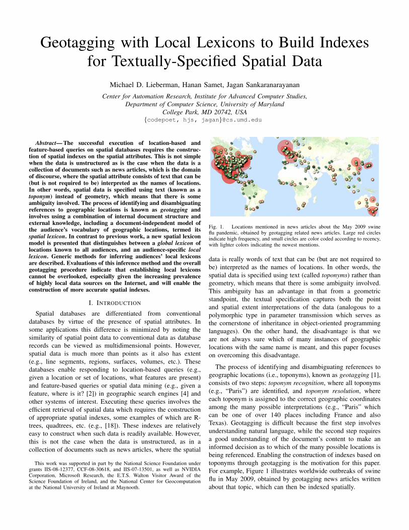
Fig. 1. Locations mentioned in news articles about the May 2009 swineflu pandemic, obtained by geotagging related news articles. Large red circlesindicate high frequency, and small circles are color coded according to recency,with lighter colors indicating the newest mentions.

data is really words of text that can be (but are not required to

be) interpreted as the names of locations. In other words, the

spatial data is specified using text (called toponyms) rather than

geometry, which means that there is some ambiguity involved.

This ambiguity has an advantage in that from a geometric

standpoint, the textual specification captures both the point

and spatial extent interpretations of the data (analogous to a

polymorphic type in parameter transmission which serves as

the cornerstone of inheritance in object-oriented programming

languages). On the other hand, the disadvantage is that we

are not always sure which of many instances of geographic

locations with the same name is meant, and this paper focuses

on overcoming this disadvantage.

The process of identifying and disambiguating references to

geographic locations (i.e., toponyms), known as geotagging [1],

consists of two steps: toponym recognition, where all toponyms

(e.g., “Paris”) are identified, and toponym resolution, where

each toponym is assigned to the correct geographic coordinates

among the many possible interpretations (e.g., “Paris” which

can be one of over 140 places including France and also

Texas). Geotagging is difficult because the first step involves

understanding natural language, while the second step requires

a good understanding of the document’s content to make an

informed decision as to which of the many possible locations is

being referenced. Enabling the construction of indexes based on

toponyms through geotagging is the motivation for this paper.

For example, Figure 1 illustrates worldwide outbreaks of swine

flu in May 2009, obtained by geotagging news articles written

about that topic, which can then be indexed spatially.

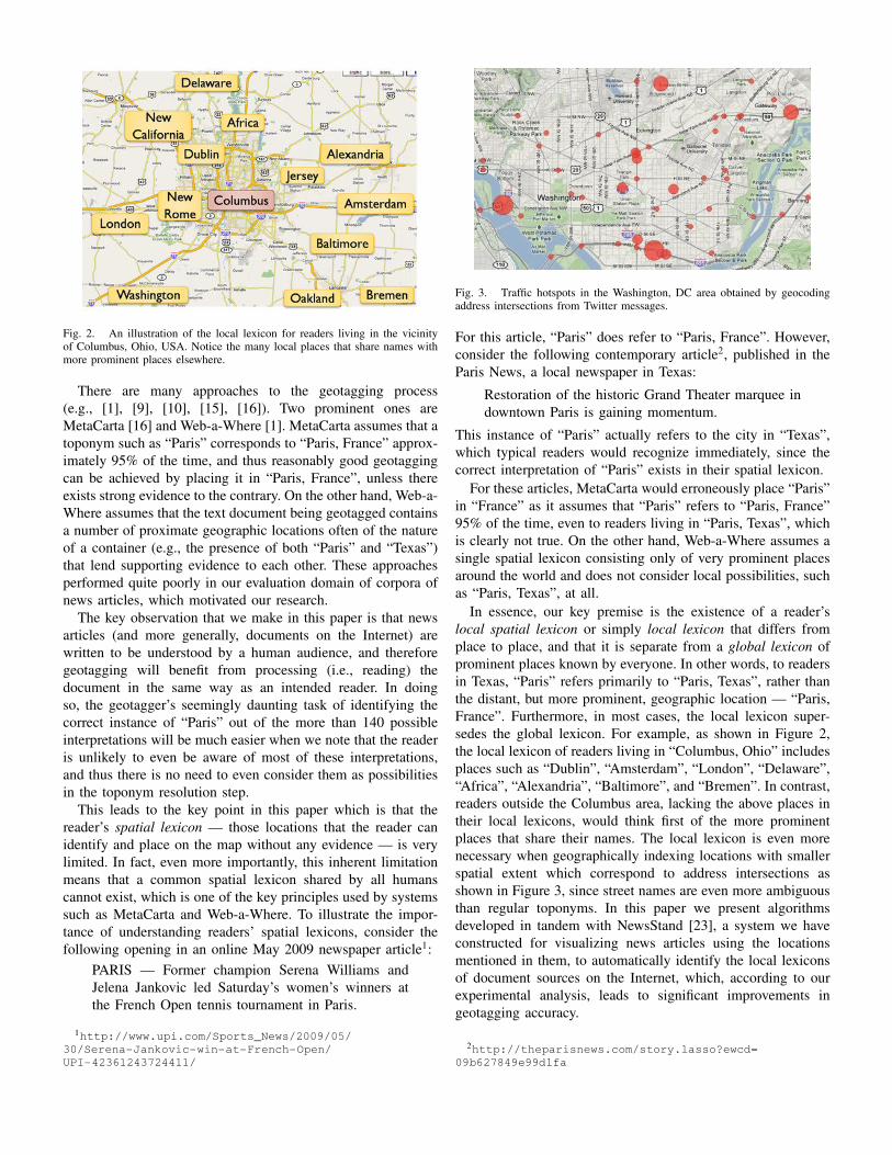
Fig. 2. An illustration of the local lexicon for readers living in the vicinityof Columbus, Ohio, USA. Notice the many local places that share names withmore prominent places elsewhere.

There are many approaches to the geotagging process

(e.g., [1], [9], [10], [15], [16]). Two prominent ones are

MetaCarta [16] and Web-a-Where [1]. MetaCarta assumes that a

toponym such as “Paris” corresponds to “Paris, France” approx-

imately 95% of the time, and thus reasonably good geotagging

can be achieved by placing it in “Paris, France”, unless there

exists strong evidence to the contrary. On the other hand, Web-a-

Where assumes that the text document being geotagged contains

a number of proximate geographic locations often of the nature

of a container (e.g., the presence of both “Paris” and “Texas”)

that lend supporting evidence to each other. These approaches

performed quite poorly in our evaluation domain of corpora of

news articles, which motivated our research.

The key observation that we make in this paper is that news

articles (and more generally, documents on the Internet) are

written to be understood by a human audience, and therefore

geotagging will benefit from processing (i.e., reading) the

document in the same way as an intended reader. In doing

so, the geotagger’s seemingly daunting task of identifying the

correct instance of “Paris” out of the more than 140 possible

interpretations will be much easier when we note that the reader

is unlikely to even be aware of most of these interpretations,

and thus there is no need to even consider them as possibilities

in the toponym resolution step.

This leads to the key point in this paper which is that the

reader’s spatial lexicon — those locations that the reader can

identify and place on the map without any evidence — is very

limited. In fact, even more importantly, this inherent limitation

means that a common spatial lexicon shared by all humans

cannot exist, which is one of the key principles used by systems

such as MetaCarta and Web-a-Where. To illustrate the impor-

tance of understanding readers’ spatial lexicons, consider the

following opening in an online May 2009 newspaper article1:

PARIS — Former champion Serena Williams and

Jelena Jankovic led Saturday’s women’s winners at

the French Open tennis tournament in Paris.

1http://www.upi.com/Sports_News/2009/05/

30/Serena-Jankovic-win-at-French-Open/

UPI-42361243724411/

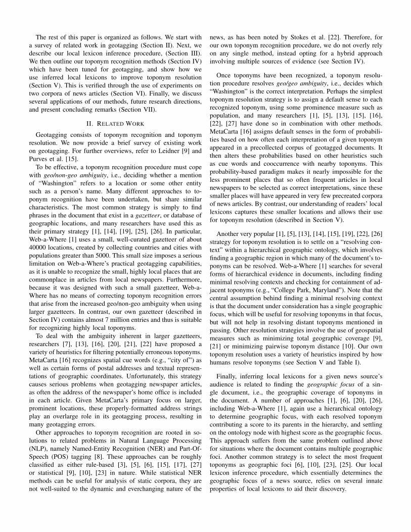
Fig. 3. Traffic hotspots in the Washington, DC area obtained by geocodingaddress intersections from Twitter messages.

For this article, “Paris” does refer to “Paris, France”. However,

consider the following contemporary article2, published in the

Paris News, a local newspaper in Texas:

Restoration of the historic Grand Theater marquee in

downtown Paris is gaining momentum.

This instance of “Paris” actually refers to the city in “Texas”,

which typical readers would recognize immediately, since the

correct interpretation of “Paris” exists in their spatial lexicon.

For these articles, MetaCarta would erroneously place “Paris”

in “France” as it assumes that “Paris” refers to “Paris, France”

95% of the time, even to readers living in “Paris, Texas”, which

is clearly not true. On the other hand, Web-a-Where assumes a

single spatial lexicon consisting only of very prominent places

around the world and does not consider local possibilities, such

as “Paris, Texas”, at all.

In essence, our key premise is the existence of a reader’s

local spatial lexicon or simply local lexicon that differs from

place to place, and that it is separate from a global lexicon of

prominent places known by everyone. In other words, to readers

in Texas, “Paris” refers primarily to “Paris, Texas”, rather than

the distant, but more prominent, geographic location — “Paris,

France”. Furthermore, in most cases, the local lexicon super-

sedes the global lexicon. For example, as shown in Figure 2,

the local lexicon of readers living in “Columbus, Ohio” includes

places such as “Dublin”, “Amsterdam”, “London”, “Delaware”,

“Africa”, “Alexandria”, “Baltimore”, and “Bremen”. In contrast,

readers outside the Columbus area, lacking the above places in

their local lexicons, would think first of the more prominent

places that share their names. The local lexicon is even more

necessary when geographically indexing locations with smaller

spatial extent which correspond to address intersections as

shown in Figure 3, since street names are even more ambiguous

than regular toponyms. In this paper we present algorithms

developed in tandem with NewsStand [23], a system we have

constructed for visualizing news articles using the locations

mentioned in them, to automatically identify the local lexicons

of document sources on the Internet, which, according to our

experimental analysis, leads to significant improvements in

geotagging accuracy.

2http://theparisnews.com/story.lasso?ewcd=

09b627849e99d1fa

The rest of this paper is organized as follows. We start with

a survey of related work in geotagging (Section II). Next, we

describe our local lexicon inference procedure, (Section III).

We then outline our toponym recognition methods (Section IV)

which have been tuned for geotagging, and show how we

use inferred local lexicons to improve toponym resolution

(Section V). This is verified through the use of experiments on

two corpora of news articles (Section VI). Finally, we discuss

several applications of our methods, future research directions,

and present concluding remarks (Section VII).

II. RELATED WORK

Geotagging consists of toponym recognition and toponym

resolution. We now provide a brief survey of existing work

on geotagging. For further overviews, refer to Leidner [9] and

Purves et al. [15].

To be effective, a toponym recognition procedure must cope

with geo/non-geo ambiguity, i.e., deciding whether a mention

of “Washington” refers to a location or some other entity

such as a person’s name. Many different approaches to to-

ponym recognition have been undertaken, but share similar

characteristics. The most common strategy is simply to find

phrases in the document that exist in a gazetteer, or database of

geographic locations, and many researchers have used this as

their primary strategy [1], [14], [19], [25], [26]. In particular,

Web-a-Where [1] uses a small, well-curated gazetteer of about

40000 locations, created by collecting countries and cities with

populations greater than 5000. This small size imposes a serious

limitation on Web-a-Where’s practical geotagging capabilities,

as it is unable to recognize the small, highly local places that are

commonplace in articles from local newspapers. Furthermore,

because it was designed with such a small gazetteer, Web-a-

Where has no means of correcting toponym recognition errors

that arise from the increased geo/non-geo ambiguity when using

larger gazetteers. In contrast, our own gazetteer (described in

Section IV) contains almost 7 million entries and thus is suitable

for recognizing highly local toponyms.

To deal with the ambiguity inherent in larger gazetteers,

researchers [7], [13], [16], [20], [21], [22] have proposed a

variety of heuristics for filtering potentially erroneous toponyms.

MetaCarta [16] recognizes spatial cue words (e.g., “city of”) as

well as certain forms of postal addresses and textual represen-

tations of geographic coordinates. Unfortunately, this strategy

causes serious problems when geotagging newspaper articles,

as often the address of the newspaper’s home office is included

in each article. Given MetaCarta’s primary focus on larger,

prominent locations, these properly-formatted address strings

play an overlarge role in its geotagging process, resulting in

many geotagging errors.

Other approaches to toponym recognition are rooted in so-

lutions to related problems in Natural Language Processing

(NLP), namely Named-Entity Recognition (NER) and Part-Of-

Speech (POS) tagging [8]. These approaches can be roughly

classified as either rule-based [3], [5], [6], [15], [17], [27]

or statistical [9], [10], [23] in nature. While statistical NER

methods can be useful for analysis of static corpora, they are

not well-suited to the dynamic and everchanging nature of the

news, as has been noted by Stokes et al. [22]. Therefore, for

our own toponym recognition procedure, we do not overly rely

on any single method, instead opting for a hybrid approach

involving multiple sources of evidence (see Section IV).

Once toponyms have been recognized, a toponym resolu-

tion procedure resolves geo/geo ambiguity, i.e., decides which

“Washington” is the correct interpretation. Perhaps the simplest

toponym resolution strategy is to assign a default sense to each

recognized toponym, using some prominence measure such as

population, and many researchers [1], [5], [13], [15], [16],

[22], [27] have done so in combination with other methods.

MetaCarta [16] assigns default senses in the form of probabili-

ties based on how often each interpretation of a given toponym

appeared in a precollected corpus of geotagged documents. It

then alters these probabilities based on other heuristics such

as cue words and cooccurrence with nearby toponyms. This

probability-based paradigm makes it nearly impossible for the

less prominent places that so often frequent articles in local

newspapers to be selected as correct interpretations, since these

smaller places will have appeared in very few precreated corpora

of news articles. By contrast, our understanding of readers’ local

lexicons captures these smaller locations and allows their use

for toponym resolution (described in Section V).

Another very popular [1], [5], [13], [14], [15], [19], [22], [26]

strategy for toponym resolution is to settle on a “resolving con-

text” within a hierarchical geographic ontology, which involves

finding a geographic region in which many of the document’s to-

ponyms can be resolved. Web-a-Where [1] searches for several

forms of hierarchical evidence in documents, including finding

minimal resolving contexts and checking for containment of ad-

jacent toponyms (e.g., “College Park, Maryland”). Note that the

central assumption behind finding a minimal resolving context

is that the document under consideration has a single geographic

focus, which will be useful for resolving toponyms in that focus,

but will not help in resolving distant toponyms mentioned in

passing. Other resolution strategies involve the use of geospatial

measures such as minimizing total geographic coverage [9],

[21] or minimizing pairwise toponym distance [10]. Our own

toponym resolution uses a variety of heuristics inspired by how

humans resolve toponyms (see Section V and Table I).

Finally, inferring local lexicons for a given news source’s

audience is related to finding the geographic focus of a sin-

gle document, i.e., the geographic coverage of toponyms in

the document. A number of approaches [1], [6], [20], [26],

including Web-a-Where [1], again use a hierarchical ontology

to determine geographic focus, with each resolved toponym

contributing a score to its parents in the hierarchy, and settling

on the ontology node with highest score as the geographic focus.

This approach suffers from the same problem outlined above

for situations where the document contains multiple geographic

foci. Another common strategy is to select the most frequent

toponyms as geographic foci [6], [10], [23], [25]. Our local

lexicon inference procedure, which essentially determines the

geographic focus of a news source, relies on several innate

properties of local lexicons to aid their discovery.

III. INFERRING LOCAL LEXICONS

As noted earlier, an audience’s local lexicon plays a key role

in how news authors write for their audiences. We therefore

require an automated, scalable method for extracting local

lexicons from online news sources, which includes not only

online newspapers, but also the multiple millions of blogs and

Twitter users. To automatically infer local lexicons, we rely on

three key characteristics of them:

1) Stability: A local lexicon is constant across articles from

its news source.

2) Proximity: Toponyms in a local lexicon are geographi-

cally proximate.

3) Modesty: A local lexicon contains a considerable but not

excessive number of toponyms.

The first property tells us that by observing and analyzing

toponyms in a collection of articles from a news source, we

should be able to determine the local lexicon as a common

geographic theme among these articles. Note that this stability

applies not only to local lexicons, but also to global lexicons as

well. We must therefore use the second property of proximity

to distinguish between local lexicons and more general spatial

lexicons. In other words, a spatial lexicon can be classified

as a local lexicon if and only if the toponyms within it are

geographically proximate. The proximity property thus serves

as a means of filtering and validation on an audience’s local

lexicon. The final modesty property highlights the notion that

a person’s local lexicon, while limited geographically, should

at least contain several toponyms. In other words, it would be

rare for a person to know of only one or two local toponyms.

We will enforce the modesty property by specifying a minimum

local lexicon size.

Note that we may infer local lexicons for a news source in

a way analogous to geotagging a single article, but on a larger

scale. In other words, we can simply geotag each article in the

collection, thereby collecting a set of resolved toponyms, select

the most frequent toponyms in the collection, and check whether

the toponyms are geographically proximate and reasonable in

number. However, this presents a bootstrapping problem, in

that determining a local lexicon relies on correct geotagging

of individual articles in the collection, but correct geotagging

relies on knowing the local lexicon.

To break this dependency cycle, we use a geotagging process

termed fuzzy geotagging that does not fully resolve toponyms in

a single article, instead returning sets of possible interpretations

for ambiguous toponyms. Fuzzy geotagging can best be under-

stood as a variant of a traditional heuristic-based geotagging

process. In such a traditional process, a toponym recognition

system first finds the toponyms T in an article a. A gazetteer,

or database of geographic locations, is then used to associate

each t ∈ T with the set of all possible interpretations Rt

for t. Next, the geotagging process uses toponym resolution

heuristics to filter interpretations from the set of Rt. Finally,

for all t that are still ambiguous (i.e., |Rt| > 1), all but a single

“default sense” r are filtered from Rt. This default sense is

usually based on another heuristic, such as the resolution with

largest population or largest geographic scope in terms of a

geographic hierarchy. In this way, each recognized toponym

t is resolved to a single pair of geographic coordinates. To

accomplish fuzzy geotagging, the final default sense assignment

is removed. Then, for each t and r ∈ Rt, a weight wr is assigned

to r, either uniformly or using default sense heuristics. Note

that fuzzy geotagging is mostly independent of the underlying

geotagging implementation, as long as it performs reasonably

across the articles in A. Of course, a high quality underlying

geotagger will result in better performance when inferring local

lexicons. For fuzzy geotagging, we use our own toponym

recognition and resolution methods, described in Sections IV

and V, respectively. Furthermore, for each toponym t, we assign

weights uniformly among the plausible interpretations Rt, and

sum weights across all the articles in A.

Algorithm 1 Infer an intended audience’s local lexicon.

Input:Set of articles A, Maximum diameter Dmax,

Minimum lexicon size Smin

Output:Local lexicon L, or ∅ if none

1: procedure INFERLOCALLEXICON(A,Dmax, Smin)

2: G← ∅3: L← ∅4: for all a ∈ A do

5: G← G ∪ FUZZYGEOTAG(a)6: end for

7: G← ORDERBYWEIGHT(G)8: for i ∈ {1 . . . |G|} do

9: H ← CONVEXHULL(L ∪Gi)10: if DIAMETER(H) > Dmax then

11: break

12: end if

13: L← L ∪Gi

14: end for

15: if |L| < Smin then

16: L← ∅17: end if

18: return L

19: end procedure

With the above in mind, we may infer local lexicons using

Procedure INFERLOCALLEXICON, listed as Algorithm 1. The

procedure takes as input a set of articles A from a single news

source, as well as parameters Dmax, used to determine the

measure of geographic locality of an inferred spatial lexicon,

and Smin, the minimum allowed size of a local lexicon. We

determined appropriate values for these parameters experimen-

tally (described in Section VI-C). We begin by initializing a

set of resolved toponyms G and the eventual inferred local

lexicon L to the empty sets. (lines 2–3). Next, we loop over

all articles a ∈ A (lines 4–6), recognizing and resolving

toponyms from each article in turn. We subject each article a

to the aforementioned fuzzy geotagging process with Procedure

FUZZYGEOTAG, which returns a set of toponyms found in

a, and their potential interpretations and weights (line 5).

We aggregate these resolved and weighted toponyms into G,

merging repeated interpretations and summing their weights.

For example, if articles a1 . . . ak in the collection each contain

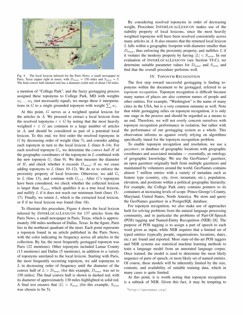
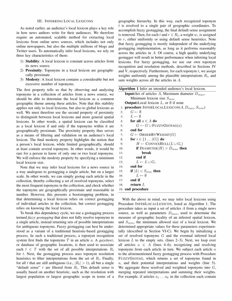
Fig. 4. The local lexicon inferred for the Paris News, a small newspaper inParis, Texas (upper right in inset), with Dmax = 150 miles and Smin = 5.The final convex hull (dashed red) has a diameter (solid red) of about 130 miles.

a mention of “College Park”, and the fuzzy geotagging process

assigned these toponyms to College Park, MD with weights

w1 . . . wk (not necessarily equal), we merge these k interpreta-

tions in G to a single grounded toponym with weight∑

iwi.

At this point, G serves as a weighted spatial lexicon for

the articles in A. We proceed to extract a local lexicon from

the resolved toponyms r ∈ G by noting that the most heavily

weighted r ∈ G are common to a large number of articles

in A, and should be considered as part of a potential local

lexicon. To this end, we first order the resolved toponyms in

G by decreasing order of weight (line 7), and consider adding

each toponym in turn to the local lexicon L (lines 8–14). For

each resolved toponym Gi, we determine the convex hull H of

the geographic coordinates of the toponyms in L combined with

the new toponym Gi (line 9). We then measure the diameter

of H , and check whether it exceeds Dmax; if so, we cease

adding toponyms to L (lines 10–12). We do so to enforce the

proximity property of local lexicons. Otherwise, we add Gi

to L (line 13), and continue with Gi+1. After G’s toponyms

have been considered, we check whether the collected lexicon

is larger than Smin, which qualifies it as a true local lexicon,

and nullify L if it does not reach our minimum limit (lines 15–

17). Finally, we return L, which is the extracted local lexicon,

or ∅ if no local lexicon was found (line 18).

To illustrate this procedure, Figure 4 shows the local lexicon

inferred by INFERLOCALLEXICON for 137 articles from the

Paris News, a small newspaper in Paris, Texas, which is approx-

imately 100 miles northeast of Dallas, Texas. In the figure, Paris

lies in the northeast quadrant of the inset. Each point represents

a toponym found in an article published in the Paris News,

with the color indicating its frequency across all articles in the

collection. By far, the most frequently geotagged toponym was

Paris (22 mentions). Other toponyms included Lamar County

(13 mentions) and Dallas (5 mentions), in addition to a variety

of toponyms unrelated to the local lexicon. Starting with Paris,

the most frequently occurring toponym, we add toponyms to

L in decreasing order of frequency until the diameter of the

convex hull of L > Dmax (for this example, Dmax was set to

150 miles). The final convex hull is shown in dashed red, with

its diameter of approximately 130 miles highlighted in solid red.

A final test ensures that |L| > Smin (for this example, Smin

was chosen to be 5).

By considering resolved toponyms in order of decreasing

weight, Procedure INFERLOCALLEXICON makes use of the

stability property of local lexicons, since the most heavily

weighted toponyms will have been resolved consistently across

many articles in A. It also ensures that the returned local lexicon

L falls within a geographic footprint with diameter smaller than

Dmax, thus enforcing the proximity property, and nullifies L if

it violates the modesty property by having |L| < Smin. In our

evaluation of INFERLOCALLEXICON (see Section VI-C), we

determine suitable parameter values for Dmax and Smin and

find that the overall procedure performs well.

IV. TOPONYM RECOGNITION

The first step toward successful geotagging is finding to-

ponyms within the document to be geotagged, referred to as

toponym recognition. Toponym recognition is difficult because

many names of places are also common names of people and

other entities. For example, “Washington” is the name of many

cities in the USA, but is a very common surname as well. Note

that while geotagging relies on toponym recognition, it is only

one stage in the process and should be regarded as a means to

an end. Therefore, we will not overly concern ourselves with

toponym recognition performance in isolation, but rather with

the performance of our geotagging system as a whole. This

observation informs us against overly relying on algorithms

specifically tuned for the toponym recognition problem.

To enable toponym recognition and resolution, we use a

gazetteer, or database of geographic locations with geographic

coordinates and associated metadata — essentially, an ontology

of geographic knowledge. We use the GeoNames3 gazetteer,

an open gazetteer originally built from multiple gazetteers and

maintained by volunteers around the world. GeoNames contains

almost 7 million entries with a variety of metadata such as

feature type (country, city, river, mountain, etc.), population,

elevation, and positions within a political geographic hierarchy.

For example, the College Park entry contains pointers to its

containers at increasing levels of scope: Prince George’s County,

Maryland, United States, North America. We store and query

the GeoNames gazetteer in a PostgreSQL database.

For toponym recognition, we also make use of approaches

built for solving problems from the natural language processing

community, and in particular the problems of Part-Of-Speech

(POS) tagging and Named-Entity Recognition (NER) [8]. The

purpose of POS tagging is to assign a part of speech to each

word given as input, while NER requires that a limited set of

typed entities (typically people, organizations, locations, dates,

etc.) are found and reported. Most state-of-the-art POS taggers

and NER systems use statistical machine learning methods to

train a language model from an annotated language corpus.

Once trained, the model is used to determine the most likely

sequence of parts of speech, or most likely set of named entities.

Of course, these models will be inherently limited by the size,

contents, and availability of suitable training data, which in

many cases is quite limited.

At this point, it is worth noting that toponym recognition

is a subtask of NER. Given this fact, it may be tempting to

3http://geonames.org/

simply use a NER system to find toponyms. However, being

a more general task, most NER systems sacrifice recall in

favor of precision (see Section VI-A for the definitions of

precision and recall). In other words, they miss many toponyms

so that the ones that they report are valid. Also, statistical NER

systems are usually trained on corpora of tagged news wire

text containing few less-prominent toponyms. As a result, the

toponyms in an NER training corpus essentially serve as a

very limited gazetteer, which in turn limits the breadth of a

toponym recognizer using models trained on the corpus. This

limitation drastically reduces their performance on articles from

local newspapers, as noted by Stokes et al. [22]. Therefore, we

do not overly rely on POS tagger and NER output, instead using

them in more advisory roles.

With this in mind, we proceed with a hybrid toponym

recognition technique. Given a news article, we tag each word

with its part of speech, using the POS tagger, and collect all

word phrases consisting of proper nouns. We also apply NER

to the article, and collect all phrases tagged as locations. As a

final measure, we gather probable toponyms using rules based

on our toponym resolution heuristics (see Table I) as well as

geographic cue words that occur frequently in news articles.

For example, phrases such as “city of X”, “just outside of

X”, “X-based”, and “X Ocean” are strong indicators that X

is a full or partial toponym. Then, for each collected phrase,

we query the gazetteer, and report phrases that exist in the

gazetteer as toponyms. We use TreeTagger4 trained on the Penn

TreeBank corpus for tagging parts of speech, and the Stanford

NLP Group’s NER system5 for finding location entities.

This optimistic toponym recognition process results in many

more reported toponyms than actually exist in the article, due

to the aforementioned ambiguity and potentially misleading

contextual geographic clues, which results in low toponym pre-

cision. However, because toponym recognition is only one part

of the geotagging process, it is most important at the toponym

recognition stage to maximize recall, since local lexicons serve

as a powerful way to filter and temper precision errors.

V. TOPONYM RESOLUTION

Having established a method for determining local lexicons,

we are now prepared to apply these lexicons for toponym

resolution. The main idea behind our geotagging process is to

model how an article author establishes a geographic framework

within an article, to make it easier for human readers in the

author’s intended audience to recognize and resolve toponyms.

Authors create this framework by using linguistic contextual

clues that we can detect using heuristic rules. Furthermore,

readers are expected to read articles linearly, so article language

has a contextual and geographic flow. Toponyms mentioned in a

sentence will establish a geographic framework for subsequent

text. To ensure correct geotagging, we therefore process the

article text in a linear fashion.

Finally, and of greatest importance, an article author will

keep in mind the nature of the expected audience’s spatial

4http://www.ims.uni-stuttgart.de/projekte/corplex/

TreeTagger/5http://nlp.stanford.edu/ner/

lexicon, and in particular the local lexicon, to underspecify

those toponyms in situations where adding geographic context

would be redundant. For these underspecified toponyms, we

will only consider those possible interpretations that are known

to intended readers, either due to relative prominence (such as

countries and capital cities) or existence in their local lexicon,

rather than all possible interpretations from the multiple millions

of entries in our gazetteer, which is a much larger set of

locations than any human could possibly know. If no resolution

is found that satisfies our constraints, we drop the toponym as

a false positive, rather than assuming the toponym recognition

process was correct and hence assigning it a default sense

(e.g., the most populous interpretation). In a more general

sense, unlike many existing geotagging approaches, we view

successful geotagging as a single integrated process, rather than

as separate toponym recognition and resolution systems that are

chained together.

After recognizing toponyms from an article to be geotagged

(see Section IV), we proceed to resolve toponyms using a

number of heuristic rules. Table I lists the set of heuristics used

in our toponym resolution process, as well as examples of when

each heuristic would be applied. These heuristics are inspired

by how humans normally read news articles. We apply the

heuristics in the order listed in Table I. For toponyms that can be

resolved by multiple heuristics, we use the resolution suggested

by the highest ranked heuristic. Our highest-ranked heuristics

establish a geographic context for large portions of the article,

i.e., Dateline (H1) and Relative Geography (H2). We continue

with heuristics favoring contextual language clues, namely

Comma Group (H3) and Location/Container (H4). Finally, we

conclude with default sense heuristics using the reader’s Local

Lexicon (H5) and Global Lexicon (H6). In addition, we use

a One Sense (H7) heuristic modeled after the “one sense per

discourse” assumption that all instances of a repeated toponym

will have the same resolution. We apply H7 after each of

H1–H6, which propagates a toponym resolution to all later

repeated mentions of the toponym. This heuristic enforces a

consistent resolution of the same toponym in the same article.

Note that despite the Local Lexicon heuristic’s low ranking as

H5, several other heuristics, namelyH1–H3, appeal to the Local

Lexicon heuristic for correct resolution. The local lexicon thus

plays a large role in our toponym resolution procedure. In our

evaluation, we measure how often each heuristic was used in

geotagging our evaluation corpora (see Section VI-E).

For the sake of clarity, we now provide more detailed

descriptions of heuristics H1–H6, and give examples of each.

H1, Dateline

We examine the article, checking for the presence of dateline

toponyms, which if present appears at the article’s beginning

and establishes the general geographic locality of the events

described in the article. If happening in a place unfamiliar to

the author’s audience, authors generally use location/container

clues (e.g., “LONDON, Ont. —”). Otherwise the location will

be underspecified (e.g., “LONDON —”), since it already exists

in the audience’s global lexicon, or frequently its local lexicon.

We therefore attempt to resolve dateline toponyms using the Lo-

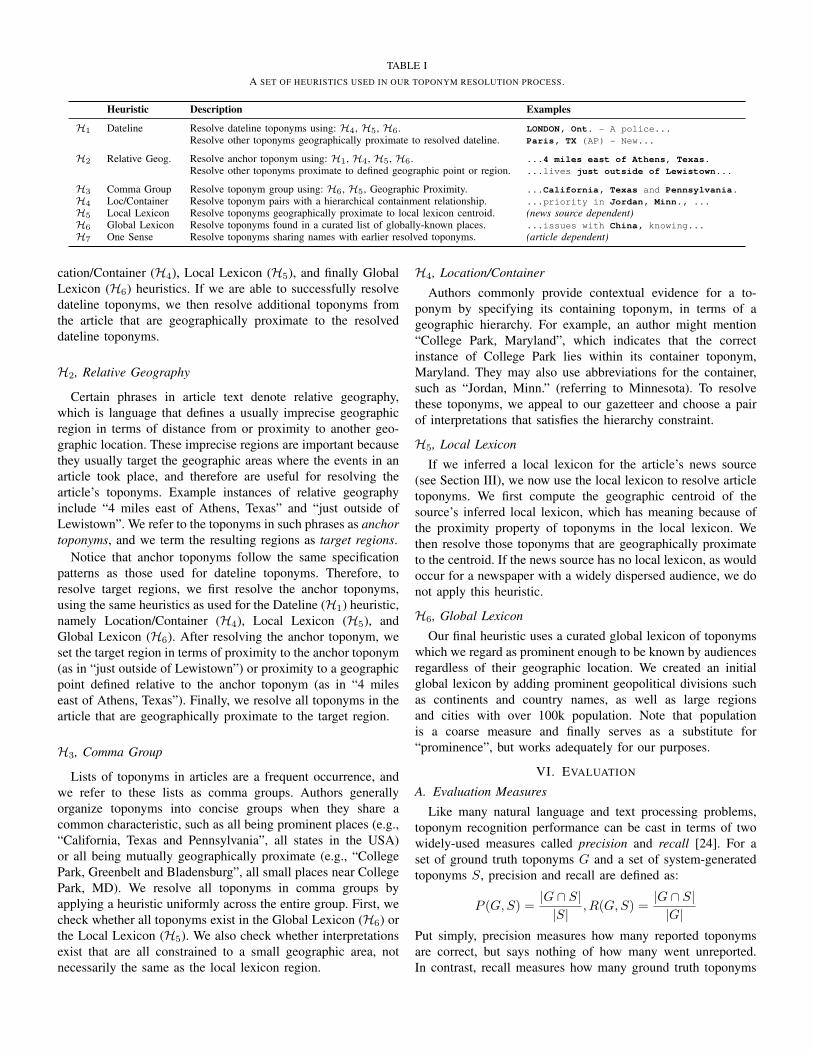
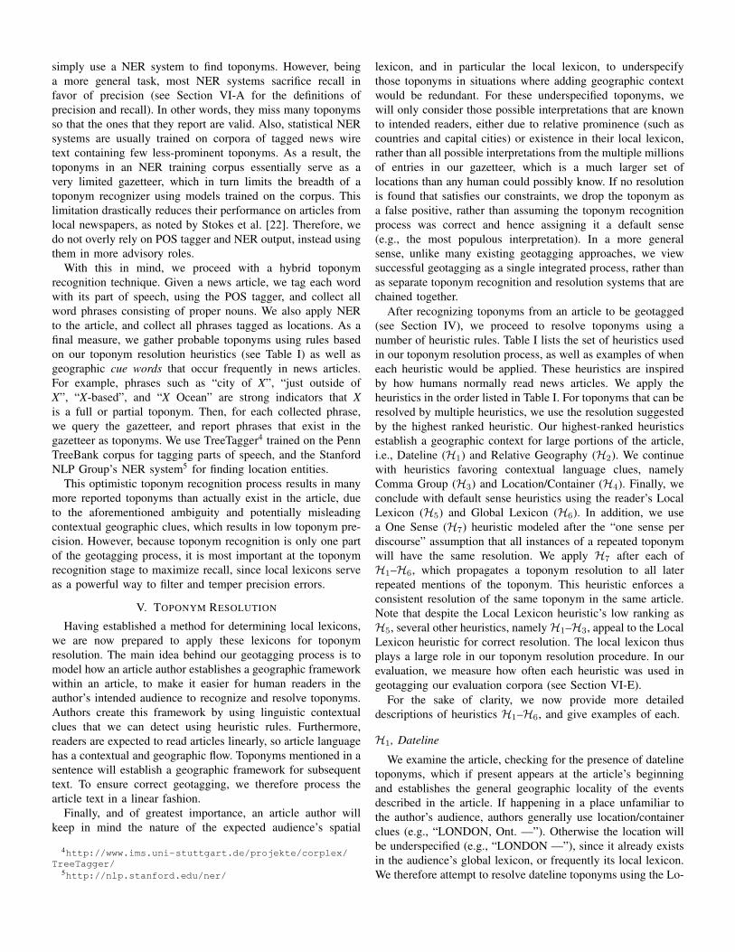
TABLE I

A SET OF HEURISTICS USED IN OUR TOPONYM RESOLUTION PROCESS.

Heuristic Description Examples

H1 Dateline Resolve dateline toponyms using: H4, H5, H6. LONDON, Ont. - A police...

Resolve other toponyms geographically proximate to resolved dateline. Paris, TX (AP) - New...

H2 Relative Geog. Resolve anchor toponym using: H1, H4, H5, H6. ...4 miles east of Athens, Texas.

Resolve other toponyms proximate to defined geographic point or region. ...lives just outside of Lewistown...

H3 Comma Group Resolve toponym group using: H6, H5, Geographic Proximity. ...California, Texas and Pennsylvania.

H4 Loc/Container Resolve toponym pairs with a hierarchical containment relationship. ...priority in Jordan, Minn., ...

H5 Local Lexicon Resolve toponyms geographically proximate to local lexicon centroid. (news source dependent)

H6 Global Lexicon Resolve toponyms found in a curated list of globally-known places. ...issues with China, knowing...

H7 One Sense Resolve toponyms sharing names with earlier resolved toponyms. (article dependent)

cation/Container (H4), Local Lexicon (H5), and finally Global

Lexicon (H6) heuristics. If we are able to successfully resolve

dateline toponyms, we then resolve additional toponyms from

the article that are geographically proximate to the resolved

dateline toponyms.

H2, Relative Geography

Certain phrases in article text denote relative geography,

which is language that defines a usually imprecise geographic

region in terms of distance from or proximity to another geo-

graphic location. These imprecise regions are important because

they usually target the geographic areas where the events in an

article took place, and therefore are useful for resolving the

article’s toponyms. Example instances of relative geography

include “4 miles east of Athens, Texas” and “just outside of

Lewistown”. We refer to the toponyms in such phrases as anchor

toponyms, and we term the resulting regions as target regions.

Notice that anchor toponyms follow the same specification

patterns as those used for dateline toponyms. Therefore, to

resolve target regions, we first resolve the anchor toponyms,

using the same heuristics as used for the Dateline (H1) heuristic,

namely Location/Container (H4), Local Lexicon (H5), and

Global Lexicon (H6). After resolving the anchor toponym, we

set the target region in terms of proximity to the anchor toponym

(as in “just outside of Lewistown”) or proximity to a geographic

point defined relative to the anchor toponym (as in “4 miles

east of Athens, Texas”). Finally, we resolve all toponyms in the

article that are geographically proximate to the target region.

H3, Comma Group

Lists of toponyms in articles are a frequent occurrence, and

we refer to these lists as comma groups. Authors generally

organize toponyms into concise groups when they share a

common characteristic, such as all being prominent places (e.g.,

“California, Texas and Pennsylvania”, all states in the USA)

or all being mutually geographically proximate (e.g., “College

Park, Greenbelt and Bladensburg”, all small places near College

Park, MD). We resolve all toponyms in comma groups by

applying a heuristic uniformly across the entire group. First, we

check whether all toponyms exist in the Global Lexicon (H6) or

the Local Lexicon (H5). We also check whether interpretations

exist that are all constrained to a small geographic area, not

necessarily the same as the local lexicon region.

H4, Location/Container

Authors commonly provide contextual evidence for a to-

ponym by specifying its containing toponym, in terms of a

geographic hierarchy. For example, an author might mention

“College Park, Maryland”, which indicates that the correct

instance of College Park lies within its container toponym,

Maryland. They may also use abbreviations for the container,

such as “Jordan, Minn.” (referring to Minnesota). To resolve

these toponyms, we appeal to our gazetteer and choose a pair

of interpretations that satisfies the hierarchy constraint.

H5, Local Lexicon

If we inferred a local lexicon for the article’s news source

(see Section III), we now use the local lexicon to resolve article

toponyms. We first compute the geographic centroid of the

source’s inferred local lexicon, which has meaning because of

the proximity property of toponyms in the local lexicon. We

then resolve those toponyms that are geographically proximate

to the centroid. If the news source has no local lexicon, as would

occur for a newspaper with a widely dispersed audience, we do

not apply this heuristic.

H6, Global Lexicon

Our final heuristic uses a curated global lexicon of toponyms

which we regard as prominent enough to be known by audiences

regardless of their geographic location. We created an initial

global lexicon by adding prominent geopolitical divisions such

as continents and country names, as well as large regions

and cities with over 100k population. Note that population

is a coarse measure and finally serves as a substitute for

“prominence”, but works adequately for our purposes.

VI. EVALUATION

A. Evaluation Measures

Like many natural language and text processing problems,

toponym recognition performance can be cast in terms of two

widely-used measures called precision and recall [24]. For a

set of ground truth toponyms G and a set of system-generated

toponyms S, precision and recall are defined as:

P (G,S) =|G ∩ S|

|S|, R(G,S) =

|G ∩ S|

|G|

Put simply, precision measures how many reported toponyms

are correct, but says nothing of how many went unreported.

In contrast, recall measures how many ground truth toponyms

TABLE II

EVALUATION CORPUS STATISTICS.

ACE LGL

Number of data sources 4 78Number of articles 104 588Number of tokens 48036 213446Number of toponyms 5813 4793Distinct toponyms 915 1297

Prevalent Toponym Types

Countries 1685 961Administrative divisions 255 1322Capital cities 454 318Populated places 178 1968

were reported and correct, but does not indicate how many of

all reported toponyms are correct.

To combine precision and recall into a single measure for

comparative purposes, we use the F1-score [24], which is

simply the harmonic mean of precision and recall:

F1 =2PR

P + R

B. Datasets

We used two datasets of news articles in our evaluation. The

first is a subset of the ACE 2005 English SpatialML Anno-

tations [11], available from the Linguistic Data Consortium,

which we will refer to as ACE. ACE contains 428 documents

in total that represent a variety of spatially-informed data

sources, including news wire and blog text, as well as online

newsgroups and transcripts of broadcast news. Each document

is annotated using SpatialML, an XML-based language which

allows the recording of toponyms and their geographically-

relevant attributes, such as their lat/lon position, feature type,

and corresponding entry in a gazetteer. For this evaluation, we

limited our test collection to news stories, resulting in 104 news

articles from prominent newspapers and news wire sources.

Unfortunately, since news wire is usually written and edited

for a broadly distributed geographic audience, the ACE corpus

is quite limited for the purposes of evaluating local lexicons’

impact on geotagging, and is hardly representative of data from

smaller newspapers with a more localized audience, which have

a large presence on the Internet. As a result, we created our own

corpus of news articles by sampling from the collection of over

4 million articles indexed by the NewsStand system [23], which

we call the Local-Global Lexicon corpus, or simply LGL. We

focused on articles from a variety of smaller, geographically-

distributed newspapers. To find this set of smaller newspapers

and thereby ensure a more challenging toponym resolution

process, we first ranked toponyms in our gazetteer by ambiguity,

and selected highly ambiguous toponyms such as Paris and Lon-

don. We then selected newspapers based near these ambiguous

toponyms. For example, some US-based newspapers located

near a Paris include the Paris News (Texas), the Paris Post-

Intelligencer (Tennessee), and the Paris Beacon-News (Illinois).

For each newspaper, we chose several articles to include in

LGL, and manually annotated the toponyms in these articles,

including the corresponding entries from our gazetteer.

TABLE III

FOR A GIVEN NEWS SOURCE N , SITUATIONS IN WHICH WE CONSIDER OUR

LOCAL LEXICON INFERENCE PROCEDURE’S FOCUS NS TO MATCH THE

GROUND TRUTH FOCUS NG .

NG exists NS exists D(NG, NS) ≤ δ Match

No No — YesYes No — NoNo Yes — NoYes Yes No NoYes Yes Yes Yes

Table II summarizes statistics for the ACE and LGL corpora.

These statistics show the limitations of ACE in terms of

source breadth, as only four news sources are represented in

the corpus — Agence France-Presse (AFP), Associated Press

World, New York Times, and Xinhua — with 42, 40, 5, and 17

annotated articles from each source, respectively. LGL contains

588 articles from 78 newspapers, with an average of 5 articles

per newspaper. Also, as the toponym counts show, the articles in

ACE tend to be more toponym-heavy, with over 50 toponyms

per article, in contrast to LGL articles with an average of 8

toponyms per article. Examining the prevalent toponym types

in both data sources reveals that the ACE collection is also

very international in scope, with 1685 of 5813 toponyms (29%)

corresponding to country names. In contrast, LGL’s set of to-

ponyms are more local. Out of 4793 total toponyms, 1968 (41%)

are smaller populated places, and 1322 (28%) are administrative

divisions such as states and counties. These statistics show that

the ACE corpus is better suited for evaluating geotagging on

an international scope, while LGL is better-suited for testing

geotagging on a local level.

C. Inferring Local Lexicons

We tested our local lexicon inference procedure with fuzzy

geotagging, described in Section III. The idea behind our

evaluation procedure is that for a small, local newspaper, the

newspaper’s audience will be geographically proximate to the

newspaper’s geographic focus. As a result, the local lexicon of

the newspaper’s audience will consist of multiple places near the

newspaper’s geographic focus. We can measure how successful

we are in establishing a given newspaper’s audience’s local

lexicon by checking whether the centroid of our inferred local

lexicon is within a given distance δ to a ground truth annotation

of the newspaper’s geographic focus. For larger newspapers

annotated with no geographic focus and hence no assumed local

lexicon, we check that our local lexicon inference procedure

also returned no local lexicon. In other words, we test our

inference procedure first in terms of binary classification (“has

local lexicon” or “no local lexicon”) and second in terms of

geographic distance from the ground truth focus. As earlier,

we use precision and recall to measure performance, with the

ground truth foci and the local lexicon foci returned by our

inference procedure serving as the ground truth and system-

generated sets, respectively.

Table III summarizes the situations in which we will consider

the ground truth NG to match our system-generated local

lexicon NS for a given news source N . We consider the results

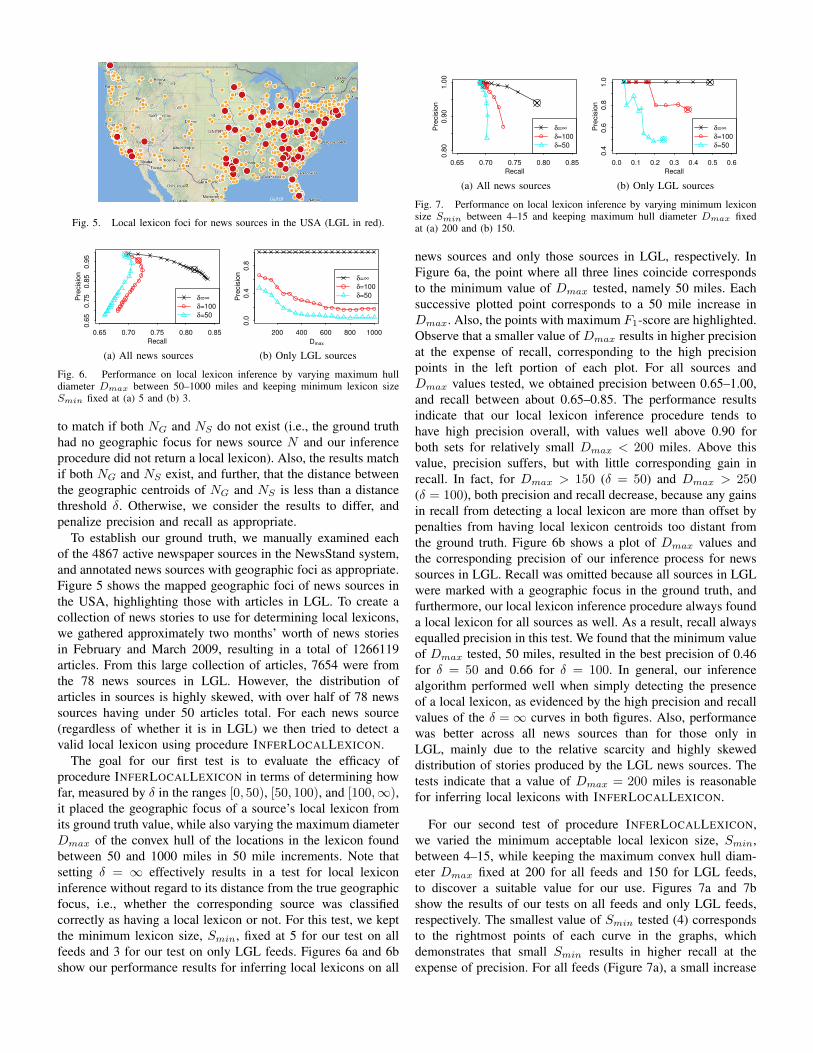
Fig. 5. Local lexicon foci for news sources in the USA (LGL in red).

0.65 0.70 0.75 0.80 0.85

0.650.750.850.95

Recall

Precision

δ=∞

δ=100

δ=50

(a) All news sources

200 400 600 800 1000

0.0

0.4

0.8

Dmax

Precision

δ=∞

δ=100

δ=50

(b) Only LGL sources

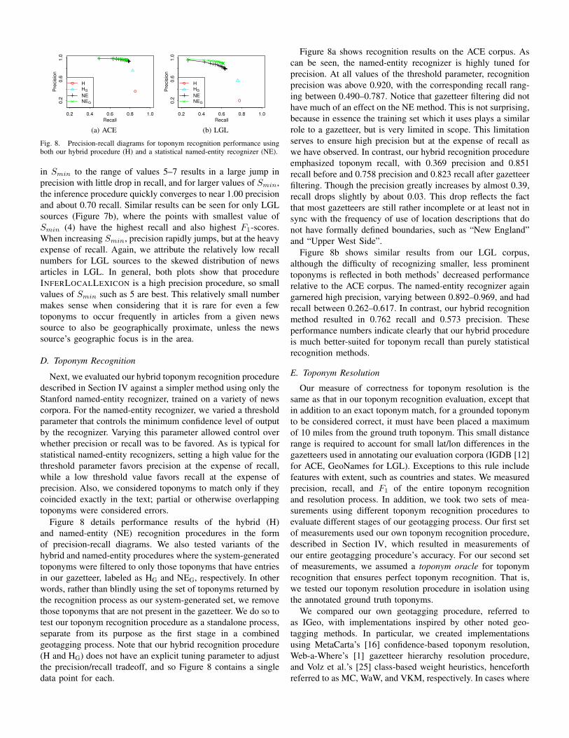
Fig. 6. Performance on local lexicon inference by varying maximum hulldiameter Dmax between 50–1000 miles and keeping minimum lexicon sizeSmin fixed at (a) 5 and (b) 3.

to match if both NG and NS do not exist (i.e., the ground truth

had no geographic focus for news source N and our inference

procedure did not return a local lexicon). Also, the results match

if both NG and NS exist, and further, that the distance between

the geographic centroids of NG and NS is less than a distance

threshold δ. Otherwise, we consider the results to differ, and

penalize precision and recall as appropriate.

To establish our ground truth, we manually examined each

of the 4867 active newspaper sources in the NewsStand system,

and annotated news sources with geographic foci as appropriate.

Figure 5 shows the mapped geographic foci of news sources in

the USA, highlighting those with articles in LGL. To create a

collection of news stories to use for determining local lexicons,

we gathered approximately two months’ worth of news stories

in February and March 2009, resulting in a total of 1266119

articles. From this large collection of articles, 7654 were from

the 78 news sources in LGL. However, the distribution of

articles in sources is highly skewed, with over half of 78 news

sources having under 50 articles total. For each news source

(regardless of whether it is in LGL) we then tried to detect a

valid local lexicon using procedure INFERLOCALLEXICON.

The goal for our first test is to evaluate the efficacy of

procedure INFERLOCALLEXICON in terms of determining how

far, measured by δ in the ranges [0, 50), [50, 100), and [100,∞),it placed the geographic focus of a source’s local lexicon from

its ground truth value, while also varying the maximum diameter

Dmax of the convex hull of the locations in the lexicon found

between 50 and 1000 miles in 50 mile increments. Note that

setting δ = ∞ effectively results in a test for local lexicon

inference without regard to its distance from the true geographic

focus, i.e., whether the corresponding source was classified

correctly as having a local lexicon or not. For this test, we kept

the minimum lexicon size, Smin, fixed at 5 for our test on all

feeds and 3 for our test on only LGL feeds. Figures 6a and 6b

show our performance results for inferring local lexicons on all

0.65 0.70 0.75 0.80 0.85

0.80

0.90

1.00

Recall

Precision

δ=∞

δ=100

δ=50

(a) All news sources

0.0 0.1 0.2 0.3 0.4 0.5 0.6

0.4

0.6

0.8

1.0

Recall

Precision

δ=∞

δ=100

δ=50

(b) Only LGL sources

Fig. 7. Performance on local lexicon inference by varying minimum lexiconsize Smin between 4–15 and keeping maximum hull diameter Dmax fixedat (a) 200 and (b) 150.

news sources and only those sources in LGL, respectively. In

Figure 6a, the point where all three lines coincide corresponds

to the minimum value of Dmax tested, namely 50 miles. Each

successive plotted point corresponds to a 50 mile increase in

Dmax. Also, the points with maximum F1-score are highlighted.

Observe that a smaller value of Dmax results in higher precision

at the expense of recall, corresponding to the high precision

points in the left portion of each plot. For all sources and

Dmax values tested, we obtained precision between 0.65–1.00,

and recall between about 0.65–0.85. The performance results

indicate that our local lexicon inference procedure tends to

have high precision overall, with values well above 0.90 for

both sets for relatively small Dmax < 200 miles. Above this

value, precision suffers, but with little corresponding gain in

recall. In fact, for Dmax > 150 (δ = 50) and Dmax > 250(δ = 100), both precision and recall decrease, because any gains

in recall from detecting a local lexicon are more than offset by

penalties from having local lexicon centroids too distant from

the ground truth. Figure 6b shows a plot of Dmax values and

the corresponding precision of our inference process for news

sources in LGL. Recall was omitted because all sources in LGL

were marked with a geographic focus in the ground truth, and

furthermore, our local lexicon inference procedure always found

a local lexicon for all sources as well. As a result, recall always

equalled precision in this test. We found that the minimum value

of Dmax tested, 50 miles, resulted in the best precision of 0.46

for δ = 50 and 0.66 for δ = 100. In general, our inference

algorithm performed well when simply detecting the presence

of a local lexicon, as evidenced by the high precision and recall

values of the δ =∞ curves in both figures. Also, performance

was better across all news sources than for those only in

LGL, mainly due to the relative scarcity and highly skewed

distribution of stories produced by the LGL news sources. The

tests indicate that a value of Dmax = 200 miles is reasonable

for inferring local lexicons with INFERLOCALLEXICON.

For our second test of procedure INFERLOCALLEXICON,

we varied the minimum acceptable local lexicon size, Smin,

between 4–15, while keeping the maximum convex hull diam-

eter Dmax fixed at 200 for all feeds and 150 for LGL feeds,

to discover a suitable value for our use. Figures 7a and 7b

show the results of our tests on all feeds and only LGL feeds,

respectively. The smallest value of Smin tested (4) corresponds

to the rightmost points of each curve in the graphs, which

demonstrates that small Smin results in higher recall at the

expense of precision. For all feeds (Figure 7a), a small increase

0.2 0.4 0.6 0.8 1.0

0.2

0.6

1.0

Recall

Precision

H

HG

NE

NEG

(a) ACE

0.2 0.4 0.6 0.8 1.0

0.2

0.6

1.0

Recall

Precision

H

HG

NE

NEG

(b) LGL

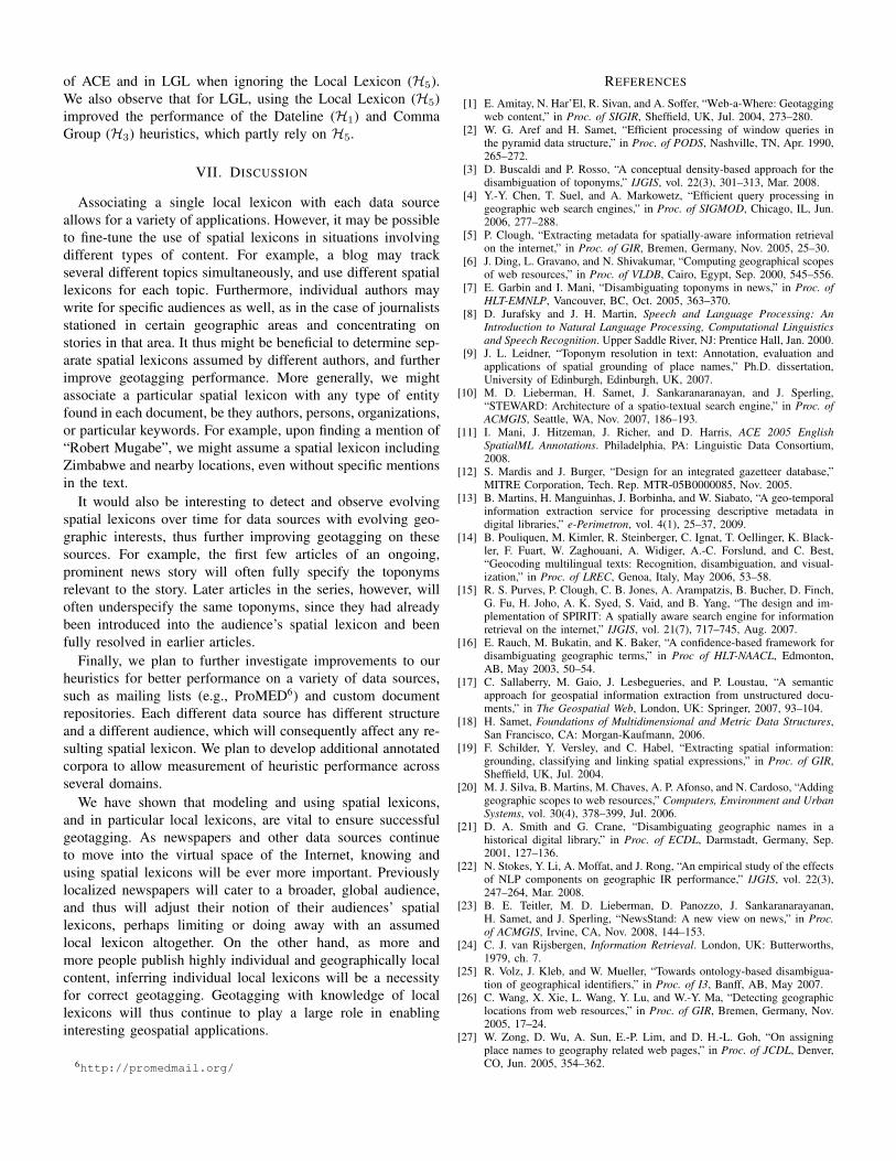
Fig. 8. Precision-recall diagrams for toponym recognition performance usingboth our hybrid procedure (H) and a statistical named-entity recognizer (NE).

in Smin to the range of values 5–7 results in a large jump in

precision with little drop in recall, and for larger values of Smin,

the inference procedure quickly converges to near 1.00 precision

and about 0.70 recall. Similar results can be seen for only LGL

sources (Figure 7b), where the points with smallest value of

Smin (4) have the highest recall and also highest F1-scores.

When increasing Smin, precision rapidly jumps, but at the heavy

expense of recall. Again, we attribute the relatively low recall

numbers for LGL sources to the skewed distribution of news

articles in LGL. In general, both plots show that procedure

INFERLOCALLEXICON is a high precision procedure, so small

values of Smin such as 5 are best. This relatively small number

makes sense when considering that it is rare for even a few

toponyms to occur frequently in articles from a given news

source to also be geographically proximate, unless the news

source’s geographic focus is in the area.

D. Toponym Recognition

Next, we evaluated our hybrid toponym recognition procedure

described in Section IV against a simpler method using only the

Stanford named-entity recognizer, trained on a variety of news

corpora. For the named-entity recognizer, we varied a threshold

parameter that controls the minimum confidence level of output

by the recognizer. Varying this parameter allowed control over

whether precision or recall was to be favored. As is typical for

statistical named-entity recognizers, setting a high value for the

threshold parameter favors precision at the expense of recall,

while a low threshold value favors recall at the expense of

precision. Also, we considered toponyms to match only if they

coincided exactly in the text; partial or otherwise overlapping

toponyms were considered errors.

Figure 8 details performance results of the hybrid (H)

and named-entity (NE) recognition procedures in the form

of precision-recall diagrams. We also tested variants of the

hybrid and named-entity procedures where the system-generated

toponyms were filtered to only those toponyms that have entries

in our gazetteer, labeled as HG and NEG, respectively. In other

words, rather than blindly using the set of toponyms returned by

the recognition process as our system-generated set, we remove

those toponyms that are not present in the gazetteer. We do so to

test our toponym recognition procedure as a standalone process,

separate from its purpose as the first stage in a combined

geotagging process. Note that our hybrid recognition procedure

(H and HG) does not have an explicit tuning parameter to adjust

the precision/recall tradeoff, and so Figure 8 contains a single

data point for each.

Figure 8a shows recognition results on the ACE corpus. As

can be seen, the named-entity recognizer is highly tuned for

precision. At all values of the threshold parameter, recognition

precision was above 0.920, with the corresponding recall rang-

ing between 0.490–0.787. Notice that gazetteer filtering did not

have much of an effect on the NE method. This is not surprising,

because in essence the training set which it uses plays a similar

role to a gazetteer, but is very limited in scope. This limitation

serves to ensure high precision but at the expense of recall as

we have observed. In contrast, our hybrid recognition procedure

emphasized toponym recall, with 0.369 precision and 0.851

recall before and 0.758 precision and 0.823 recall after gazetteer

filtering. Though the precision greatly increases by almost 0.39,

recall drops slightly by about 0.03. This drop reflects the fact

that most gazetteers are still rather incomplete or at least not in

sync with the frequency of use of location descriptions that do

not have formally defined boundaries, such as “New England”

and “Upper West Side”.

Figure 8b shows similar results from our LGL corpus,

although the difficulty of recognizing smaller, less prominent

toponyms is reflected in both methods’ decreased performance

relative to the ACE corpus. The named-entity recognizer again

garnered high precision, varying between 0.892–0.969, and had

recall between 0.262–0.617. In contrast, our hybrid recognition

method resulted in 0.762 recall and 0.573 precision. These

performance numbers indicate clearly that our hybrid procedure

is much better-suited for toponym recall than purely statistical

recognition methods.

E. Toponym Resolution

Our measure of correctness for toponym resolution is the

same as that in our toponym recognition evaluation, except that

in addition to an exact toponym match, for a grounded toponym

to be considered correct, it must have been placed a maximum

of 10 miles from the ground truth toponym. This small distance

range is required to account for small lat/lon differences in the

gazetteers used in annotating our evaluation corpora (IGDB [12]

for ACE, GeoNames for LGL). Exceptions to this rule include

features with extent, such as countries and states. We measured

precision, recall, and F1 of the entire toponym recognition

and resolution process. In addition, we took two sets of mea-

surements using different toponym recognition procedures to

evaluate different stages of our geotagging process. Our first set

of measurements used our own toponym recognition procedure,

described in Section IV, which resulted in measurements of

our entire geotagging procedure’s accuracy. For our second set

of measurements, we assumed a toponym oracle for toponym

recognition that ensures perfect toponym recognition. That is,

we tested our toponym resolution procedure in isolation using

the annotated ground truth toponyms.

We compared our own geotagging procedure, referred to

as IGeo, with implementations inspired by other noted geo-

tagging methods. In particular, we created implementations

using MetaCarta’s [16] confidence-based toponym resolution,

Web-a-Where’s [1] gazetteer hierarchy resolution procedure,

and Volz et al.’s [25] class-based weight heuristics, henceforth

referred to as MC, WaW, and VKM, respectively. In cases where

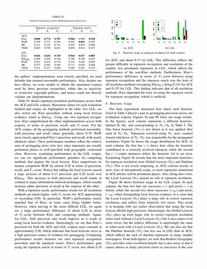
TABLE IV

TOPONYM RESOLUTION PERFORMANCE RESULTS.

Toponym recognition Toponym oracleP R F1 P R F1

ACEIGeo 0.800 0.774 0.787 0.968 0.890 0.928WaW 0.795 0.773 0.784 0.962 0.891 0.925MC 0.731 0.752 0.741 0.945 0.870 0.906VKM 0.603 0.709 0.652 0.859 0.816 0.837

LGLIGeo 0.826 0.654 0.730 0.964 0.817 0.885

IGeoNL 0.698 0.450 0.548 0.788 0.546 0.645WaW 0.651 0.452 0.534 0.761 0.628 0.689MC 0.477 0.494 0.485 0.712 0.629 0.668VKM 0.351 0.475 0.404 0.590 0.567 0.578

the authors’ implementations were loosely specified, we used

defaults that ensured reasonable performance. Also, despite our

best efforts, we were unable to obtain the annotated corpora

used by these previous researchers, either due to inactivity

or restrictive copyright policies, and hence could not directly

validate our implementations.

Table IV details toponym resolution performance across both

the ACE and LGL corpora. Maximum values for each evaluation

method and corpus are highlighted in the table. For LGL, we

also tested our IGeo procedure without using local lexicon

evidence, listed as IGeoNL. Using our own toponym recogni-

tion, IGeo outperformed the other implementations across both

corpora, in terms of precision, recall, and F1-score. For the

ACE corpus, all the geotagging methods performed reasonably,

with precision and recall values generally above 0.70. WaW

most closely approached IGeo’s precision and recall, with nearly

identical values. These performance numbers reflect the relative

ease of geotagging news wire text, since toponyms are usually

prominent places or well-specified with geographic contextual

clues. However, examining performance in the LGL corpus,

we can see significant performance penalties for competing

methods that neglect the local lexicon. IGeo outperforms its

nearest competitor WaW by almost 0.20 in terms of precision,

recall, and F1-score. Notice that adding the local lexicon caused

a large increase of about 0.13 precision and 0.20 recall over

IGeoNL. This increase in both precision and recall stands in

contrast to many information retrieval techniques, which usually

increase either precision or recall at the expense of the other.

With a toponym oracle, performance results for all resolution

methods are much higher, with F1-scores for ACE approaching

or exceeding 0.90. In particular, WaW’s performance nearly

matched that of IGeo, in some cases being slightly better.

However, when moving to the more difficult LGL, we again

see a large performance difference of about 0.20 in terms

of F1-score between IGeo and competing methods. Again,

for LGL, both precision and recall improve as a result of

using local lexicon evidence. Interestingly, we see that IGeo’s

precision for both the ACE and LGL corpora stays constant at

approximately 0.96, which indicates that local lexicons serve as

a high precision source of evidence for geotagging. Comparing

performance results between our own toponym recognition

procedure and the toponym oracle, IGeo’s performance gain

using the toponym oracle in terms of F1-score was about 0.10

H1 H2 H3 H4 H5 H6

0400

8001200

+

−

(a) ACE

H1 H2 H3 H4 H5 H6

04008001200 +

−

+NL

−NL

(b) LGL

Fig. 9. Heuristic usage in toponym resolution for both corpora.

for ACE, and about 0.15 for LGL. This difference reflects the

greater difficulty in toponym recognition and resolution of the

smaller, less prominent toponyms in LGL, which affects the

performance of the non-IGeo methods. Furthermore, IGeo’s

performance difference in terms of F1-score between using

toponym recognition and the toponym oracle was the least of

all resolution methods (excepting IGeoNL), being 0.141 for ACE

and 0.155 for LGL. This finding indicates that of all resolution

methods, IGeo depended the least on using the toponym oracle

for toponym recognition, which is artificial.

F. Heuristic Usage

Our final experiment measured how much each heuristic

listed in Table I played a part in geotagging precision across our

evaluation corpora. Figures 9a and 9b show our usage results.

In the figures, each column represents a different heuristic,

labeled H1–H6, and corresponding to H1–H6 in Table I. The

One Sense heuristic (H7) is not shown as it was applied after

each of H1–H6. Toponyms resolved using H7 were counted

toward whichever of H1–H6 was responsible for the propagated

resolution. Figure 9a shows the usage distribution for ACE. In

each column, the first bar (+) shows how often the heuristic

contributed to a correctly resolved toponym, while the second

bar (−) counts instances where the heuristic led to an error.

Examining Figure 9a reveals that the most important heuristics

for toponym resolution were Global Lexicon (H6) and Dateline

(H1). This is not overly surprising, as ACE consists mostly of

news wire of international scope, so most toponyms mentioned

in ACE articles will be prominent places. Also, being news wire,

the Local Lexicon (H5) played no role in toponym resolution.

Figure 9b shows heuristic usage in the LGL corpus. In each

column, the first two bars are successes (+) and errors (−) as

before, while the second two show successes (+NL) and errors

(−NL) when disregarding local lexicon evidence. It is clear that

the Local Lexicon (H5) plays a large role in correct toponym

resolution, and suffers from relatively few errors. This result

is in keeping with our earlier observation that using the local

lexicon affords high precision. Interestingly, the Global Lexicon

(H6) plays an even larger role in correct toponym resolution

when used without a Local Lexicon (H5) but it also causes even

more errors, but the relative difference is surprisingly the same

as when used with a Local Lexicon (H5). We can also see that

the Dateline heuristic (H1) has less use in LGL than in ACE,

which reflects the lack of dateline toponyms in many smaller

newspapers. From both figures, we note that Relative Geography

(H2) provides some resolution benefit, but is also noisy in that it

causes almost as many precision errors as successes in the case

of ACE and in LGL when ignoring the Local Lexicon (H5).

We also observe that for LGL, using the Local Lexicon (H5)

improved the performance of the Dateline (H1) and Comma

Group (H3) heuristics, which partly rely on H5.

VII. DISCUSSION

Associating a single local lexicon with each data source

allows for a variety of applications. However, it may be possible

to fine-tune the use of spatial lexicons in situations involving

different types of content. For example, a blog may track

several different topics simultaneously, and use different spatial

lexicons for each topic. Furthermore, individual authors may

write for specific audiences as well, as in the case of journalists

stationed in certain geographic areas and concentrating on

stories in that area. It thus might be beneficial to determine sep-

arate spatial lexicons assumed by different authors, and further

improve geotagging performance. More generally, we might

associate a particular spatial lexicon with any type of entity

found in each document, be they authors, persons, organizations,

or particular keywords. For example, upon finding a mention of

“Robert Mugabe”, we might assume a spatial lexicon including

Zimbabwe and nearby locations, even without specific mentions

in the text.

It would also be interesting to detect and observe evolving

spatial lexicons over time for data sources with evolving geo-

graphic interests, thus further improving geotagging on these

sources. For example, the first few articles of an ongoing,

prominent news story will often fully specify the toponyms

relevant to the story. Later articles in the series, however, will

often underspecify the same toponyms, since they had already

been introduced into the audience’s spatial lexicon and been

fully resolved in earlier articles.

Finally, we plan to further investigate improvements to our

heuristics for better performance on a variety of data sources,

such as mailing lists (e.g., ProMED6) and custom document

repositories. Each different data source has different structure

and a different audience, which will consequently affect any re-

sulting spatial lexicon. We plan to develop additional annotated

corpora to allow measurement of heuristic performance across

several domains.

We have shown that modeling and using spatial lexicons,

and in particular local lexicons, are vital to ensure successful

geotagging. As newspapers and other data sources continue

to move into the virtual space of the Internet, knowing and

using spatial lexicons will be ever more important. Previously

localized newspapers will cater to a broader, global audience,

and thus will adjust their notion of their audiences’ spatial

lexicons, perhaps limiting or doing away with an assumed

local lexicon altogether. On the other hand, as more and

more people publish highly individual and geographically local

content, inferring individual local lexicons will be a necessity

for correct geotagging. Geotagging with knowledge of local

lexicons will thus continue to play a large role in enabling

interesting geospatial applications.

6http://promedmail.org/

REFERENCES

[1] E. Amitay, N. Har’El, R. Sivan, and A. Soffer, “Web-a-Where: Geotaggingweb content,” in Proc. of SIGIR, Sheffield, UK, Jul. 2004, 273–280.

[2] W. G. Aref and H. Samet, “Efficient processing of window queries inthe pyramid data structure,” in Proc. of PODS, Nashville, TN, Apr. 1990,265–272.

[3] D. Buscaldi and P. Rosso, “A conceptual density-based approach for thedisambiguation of toponyms,” IJGIS, vol. 22(3), 301–313, Mar. 2008.

[4] Y.-Y. Chen, T. Suel, and A. Markowetz, “Efficient query processing ingeographic web search engines,” in Proc. of SIGMOD, Chicago, IL, Jun.2006, 277–288.

[5] P. Clough, “Extracting metadata for spatially-aware information retrievalon the internet,” in Proc. of GIR, Bremen, Germany, Nov. 2005, 25–30.

[6] J. Ding, L. Gravano, and N. Shivakumar, “Computing geographical scopesof web resources,” in Proc. of VLDB, Cairo, Egypt, Sep. 2000, 545–556.

[7] E. Garbin and I. Mani, “Disambiguating toponyms in news,” in Proc. ofHLT-EMNLP, Vancouver, BC, Oct. 2005, 363–370.

[8] D. Jurafsky and J. H. Martin, Speech and Language Processing: AnIntroduction to Natural Language Processing, Computational Linguistics

and Speech Recognition. Upper Saddle River, NJ: Prentice Hall, Jan. 2000.[9] J. L. Leidner, “Toponym resolution in text: Annotation, evaluation and

applications of spatial grounding of place names,” Ph.D. dissertation,University of Edinburgh, Edinburgh, UK, 2007.

[10] M. D. Lieberman, H. Samet, J. Sankaranaranayan, and J. Sperling,“STEWARD: Architecture of a spatio-textual search engine,” in Proc. ofACMGIS, Seattle, WA, Nov. 2007, 186–193.

[11] I. Mani, J. Hitzeman, J. Richer, and D. Harris, ACE 2005 EnglishSpatialML Annotations. Philadelphia, PA: Linguistic Data Consortium,2008.

[12] S. Mardis and J. Burger, “Design for an integrated gazetteer database,”MITRE Corporation, Tech. Rep. MTR-05B0000085, Nov. 2005.

[13] B. Martins, H. Manguinhas, J. Borbinha, and W. Siabato, “A geo-temporalinformation extraction service for processing descriptive metadata indigital libraries,” e-Perimetron, vol. 4(1), 25–37, 2009.

[14] B. Pouliquen, M. Kimler, R. Steinberger, C. Ignat, T. Oellinger, K. Black-ler, F. Fuart, W. Zaghouani, A. Widiger, A.-C. Forslund, and C. Best,“Geocoding multilingual texts: Recognition, disambiguation, and visual-ization,” in Proc. of LREC, Genoa, Italy, May 2006, 53–58.

[15] R. S. Purves, P. Clough, C. B. Jones, A. Arampatzis, B. Bucher, D. Finch,G. Fu, H. Joho, A. K. Syed, S. Vaid, and B. Yang, “The design and im-plementation of SPIRIT: A spatially aware search engine for informationretrieval on the internet,” IJGIS, vol. 21(7), 717–745, Aug. 2007.

[16] E. Rauch, M. Bukatin, and K. Baker, “A confidence-based framework fordisambiguating geographic terms,” in Proc of HLT-NAACL, Edmonton,AB, May 2003, 50–54.

[17] C. Sallaberry, M. Gaio, J. Lesbegueries, and P. Loustau, “A semanticapproach for geospatial information extraction from unstructured docu-ments,” in The Geospatial Web, London, UK: Springer, 2007, 93–104.

[18] H. Samet, Foundations of Multidimensional and Metric Data Structures,San Francisco, CA: Morgan-Kaufmann, 2006.

[19] F. Schilder, Y. Versley, and C. Habel, “Extracting spatial information:grounding, classifying and linking spatial expressions,” in Proc. of GIR,Sheffield, UK, Jul. 2004.

[20] M. J. Silva, B. Martins, M. Chaves, A. P. Afonso, and N. Cardoso, “Addinggeographic scopes to web resources,” Computers, Environment and UrbanSystems, vol. 30(4), 378–399, Jul. 2006.

[21] D. A. Smith and G. Crane, “Disambiguating geographic names in ahistorical digital library,” in Proc. of ECDL, Darmstadt, Germany, Sep.2001, 127–136.

[22] N. Stokes, Y. Li, A. Moffat, and J. Rong, “An empirical study of the effectsof NLP components on geographic IR performance,” IJGIS, vol. 22(3),247–264, Mar. 2008.

[23] B. E. Teitler, M. D. Lieberman, D. Panozzo, J. Sankaranarayanan,H. Samet, and J. Sperling, “NewsStand: A new view on news,” in Proc.of ACMGIS, Irvine, CA, Nov. 2008, 144–153.

[24] C. J. van Rijsbergen, Information Retrieval. London, UK: Butterworths,1979, ch. 7.

[25] R. Volz, J. Kleb, and W. Mueller, “Towards ontology-based disambigua-tion of geographical identifiers,” in Proc. of I3, Banff, AB, May 2007.

[26] C. Wang, X. Xie, L. Wang, Y. Lu, and W.-Y. Ma, “Detecting geographiclocations from web resources,” in Proc. of GIR, Bremen, Germany, Nov.2005, 17–24.

[27] W. Zong, D. Wu, A. Sun, E.-P. Lim, and D. H.-L. Goh, “On assigningplace names to geography related web pages,” in Proc. of JCDL, Denver,CO, Jun. 2005, 354–362.