
SIMPLIFYING WATERSHED MODELING
A Dissertation
Presented to the Faculty of the Graduate School
of Cornell University
In Partial Fulfillment of the Requirements for the Degree of
Doctor of Philosophy
by
Daniel Richard Fuka
January 2013

© 2013 Daniel Richard Fuka

SIMPLIFYING WATERSHED MODELING
Daniel Richard Fuka, Ph. D.
Cornell University 2013
Obtaining representative meteorological data for an area, properly characterizing the
physical characteristics of a watershed, and accurately representing the processes
internal to watersheds can be complex. Several studies are presented that simplify the
steps to obtain representative weather data, characterize the topography a watershed,
and use this physical characterization to build a process based snowmelt model that
requires no calibration to replace a calibration dependent temperature index based
model. The objective of these studies is to present a suite of computational tools and
proof of concept studies that simplify watershed modeling. First we present a method
to quickly and easily obtain a 32-year record of meteorological forcing data for any
location in the from the freely available Climate Forecast System Reanalysis dataset.
Results from this analysis indicate that the CFSR data can reliably act as a first
approximation of historical weather data over a watershed. The data consisting of
precipitation, temperature, and other relevant weather information. Results show that
using this dataset, can be as, or more, accurate than using weather records from the
closest weather stations when using the Soil and Water Assessment Tool (SWAT)
watershed model. The next two chapters describe two original software releases
intended to provide watershed modeler with a suite of computational tools to better
describe physical and chemical characteristics of a given watershed. The first,
TopoSWAT, is a toolbox intended to characterize the topological properties of
hydrological systems, and the second, SWATmodel, is an open-project porting of the

legacy SWAT watershed model to be widely distributed and run as a linear-model-like
function on multiple operating systems (OS) and processor platforms within the R
language. These software packages have resulted in significant simplification of the
integration of physical characteristics into the SWAT modeling system and have made
the SWAT modeling framework available to more users in multiple environments
including those scientists dependent on the Unix and Mac Osx based operating
systems. The final chapter presents an integration example of the previous chapters,
building a more process-based snow accumulation and snowmelt routine to replace the
temperature index based routine in the aforementioned SWAT modeling system. The
results of this integration show that spatial snow distributions predicted by a more
process-based model better matched observations from LandSat imagery and a
SNOTEL station, and requires limited extra effort when initialized using the
previously described TopoSWAT toolbox.

iii
BIOGRAPHICAL SKETCH
Daniel Richard Fuka was born in Austin, TX, the youngest of four, to Mary and Louis
Fuka. He grew up in New Mexico, and in 1991, obtained is B.S. in Horticulture from
New Mexico State University. Daniel continued on to get his M.S. Engineering degree
from Washington State University in 1995. From 1995 till 2010 Daniel moved his
research into the private sector, first hired on as a research scientist and engineer at
Quetzal Computation Associates, later Quetzal Biomedical Associates, and then in
2000 partnered in the weather commodities research group that would become
Weather Insight, LLC. During this time the research group partnered and Daniel took
on positions in the Air Routing Group companies and later Rockwell Collins. Not to
be overlooked is the amazing partnership Daniel entered into when he met Melissa in
1995, who would become his loving and extremely patient wife in 1997, and who
would understand the selling of the corporate partnerships, abandoning a great job,
and moving to Ithaca, NY in 2010 to complete the mid-life crisis that is recapitulated
in the following Dissertation.

iv
Dedicated to John K. Prentice.
Without you, this chapter of my life would never have been written.
We loved you so much.

v
ACKNOWLEDGMENTS
First, I would like to acknowledge my wife, who supported me mentally, emotionally,
and financially though this degree with little hesitation. I’d also like to thank my
Mother and Father, who never doubted that I would be finished in a few months and
never reminded me that the answer had not changed for years. Thanks to my sister
Mary for reminding me every two weeks that I was not yet finished. Thanks to my
friends in the soil and water lab especially Amy, Zachary, Brian and Ekrem who kept
me balanced, and the friends I made working and teaching in Ethiopia. I want to thank
my patient coauthors Todd, Art, Charlotte, and especially Tammo, as without him
taking on special needs cases like myself, the opportunity start this degree would
never have been possible.
Not to be overlooked is the support of Nancy, Debbi, Tami, Peggy, Steve Pacenka, as
well as Jean Hunter and Brian Richards who helped me stay inside the box while
thinking outside the box, and of course all the folks in Riley Robb that made life
especially wonderful.

vi
TABLE OF CONTENTS Biographical Sketch ....................................... .............................................................. iii Acknowledgements ....................................... ............................................................... v Table of Contents .......................................... .............................................................. vi List of Figures ................................................ ............................................................. vii List of Tables ................................................. ............................................................... x Chapter 1 ....................................................... ............................................................... 1
Introduction Chapter 2 ....................................................... ............................................................. 11
Using the Climate Forecast System Reanalysis as Weather Input Data for Watershed Models
Chapter 3 ....................................................... ............................................................. 46 The TopoSWAT Toolbox: Inclusion of Topographic Controls in ArcSWAT initialization
Chapter 4 ....................................................... ............................................................. 73
SWATmodel: A Multi-OS, Multi-Platform SWAT Model Package in R Chapter 5 ....................................................... ............................................................. 78
A Simple Process-Based Snowmelt Routine to Model Spatially Distributed Snow Depth and Snowmelt in the SWAT Model
Appendix A ................................................... ........................................................... 112
Data Sources for Chapter 2 Appendix B .................................................... ........................................................... 113
R Code Segments for Chapter 4 Appendix C .................................................... ........................................................... 114
A Fortran Subroutine Written in Format, Data Structure, and Paradigm of SWAT2005 and SWAT2009 Source Code for Chapter 5

vii
LIST OF FIGURES
Figure 2.1a-c. ................................................ ............................................................. 24
Comparison of the simplified 9 HRU initializations in the Town Brook watershed for CFSR, a), ideal meteorological weather stations, b), and against the previous best values of the more complex SWAT model initialization shown in c). The simplified initialization performs similarly to the complex initialization, and there is a significant increase in performance when the CFSR meteorological data is used to force the SWAT model.
Figure 2.2a-b. ................................................ ............................................................. 26
Comparison of the simplified 9 HRU initializations in the Gumera watershed for CFSR a) and ideal meteorological weather stations b) and there is similar performance when the CFSR meteorological data is used to force the SWAT model vs. using the closest weather stations.
Figure 2.3. ..................................................... ............................................................. 26
Hydrographs for Town Brook (a) and Gumera (b) watersheds, showing the measured stream flow (black) with the CFSR-based prediction (red) and nearest weather station (blue).
Figure 2.4a-b. ................................................ ............................................................. 28
Comparison of the simplified 9 HRU initializations in the Cross River watershed, a) shows the CFSR meteorological data results b) and ideal meteorological weather station results used to force the SWAT model.
Figure 2.5a-b. ................................................ ............................................................. 29
Comparison of the simplified 9 HRU initializations in the Tesuque Creek Andreas Cr watershed, a) shows the CFSR meteorological data results and b) ideal meteorological weather station results used to force the SWAT model.
Figure 2.6a-b. ................................................ ............................................................. 30
Comparison of the simplified 9 HRU initializations in the Andreas Creek watershed, a) shows the CFSR meteorological data results and b) ideal meteorological weather station results used to force the SWAT model., Note, however in this case much of the good CFSR NSE performance is due to a few very large flow events.
Figure 2.7a-b. ................................................ ............................................................. 31
Hydrographs for Cross R. (a), Tesuque Cr. (b), and Andreas R. (c) showing the measured streamflow (black) with the CFSR-based prediction (red) and nearest weather station (blue).

viii
Figure 2.8a-c. ................................................ ............................................................. 32 Optimal NSE for the CFSR (x) and weather stations (circle) at various distances from the center of Cross R (a), Tesuque Cr. (b), and Andreas Cr. (c). Optimal NSE for CFSR interpolated to the center of the watershed is show with the asterisk (*) in each case. Negative distances indicate stations that are towards the Ocean (a and c only), with the exception of the “Palm Springs” station, which is placed in the negative side at -9.3km, to distinguish it from the “Palm Springs Regional Airport” station, at +8.6km. Error bars indicate +- 2 St. Dev. for 1000 bootstrap samples of predicted vs. observed results.
Figure 2.9a-b. ................................................ ............................................................. 34
Comparison of the simplified 9 HRU initializations in the Andreas Creek watershed for CFSR a) and ideal meteorological weather stations b) with extreme events shows that the CFSR meteorological data being used to force the SWAT model still performs better than using the closest weather station, though is a better representation of the lower performance when extreme events are removed as compared to Figure 2.6.
Figure 3.1. ..................................................... ............................................................. 60
Spatial corroboration of snow distribution using LandSat 7 imagery from April 3, 2008, with ovals to highlight the same area in each scene. Left frame (a): LandSat 7 image shows hillslope snow distribution. Right frame (b): A physically based snowmelt model distinctly shows linear features of hillside snow that align with the LandSat 7 imagery.
Figure 3.2a-f. ................................................ ............................................................. 62
SWAT model of Gilgel Abay, Blue Nile watershed, Ethiopia, initialized using a standard ArcSWAT setup with the FAO DSMW soil layer (a. SWAT), and with the TopoSWAT toolbox (b. TopoSoil); SWAT model outputs including runoff (c & d) and change soil moisture (e & f) for both model initializations.
Figure 5.1. ..................................................... ............................................................. 97
SWE for HRU 185, An evergreen forest at the highest elevation in the watershed for water years 2001 - 2008. Blue dotted line is SNOTEL measured, 300m above the average elevation of the highest elevation increment in the watershed, dashed brown line is BP, and orange line is optimal calibration for TI.
Figure 5.2. ..................................................... ............................................................. 99
Spatial corroboration using LandSat 7 imagery from April 3, 2008 with oval highlighting the same area in each scene. Upper left frame(a) LandSat 7 distinctly shows hillslope snow distribution. Upper right frame(b), SWAT-PB distinctly shows linear features of hillside snow that align with the LandSat 7 imagery. Lower left (c) SWAT-TI shows relatively uniform snow distribution

ix
Figure 5.3. ..................................................... ........................................................... 101 SWAT-PB model results for HRU Snow Water Equivalent (SWE), distinguished by hillslope aspect.
Figure 5.4. ..................................................... ........................................................... 103
Left(a) HRU-based comparison of SWAT-PB SWE (mm) vs LandSat 7 Channel 8 panchromatic brightness. Mean for each polygon extracted from raster LandSat 7 scene. Right (b) Raster cell based comparison of SWAT-PB SWE(mm) vs LandSat 7 Channel 8 panchromatic brightness with boxplots showing the progression of grouped means and pixel spread.

x
LIST OF TABLES Table 2.1. ...................................................... ............................................................. 13
Reanalysis datasets available to this project from the NCAR Computational and Information Systems Laboratory (CISL) Research Data Archive (RDA). All datasets include temperature. Note: Japanese 25 year, ECMWF 40 Year, and ECMWF Interim Reanalysis are restricted datasets not available to the public.
Table 2.2. ...................................................... ............................................................. 17
Calibrated parameters used for Differential Evolution Optimization, with the optimization method and parameter range, or percent deviation for optimization.
Table 2.3. ...................................................... ............................................................. 18 Table of watershed basin identifiers, characteristics and locations.
Table 2.4. ...................................................... ............................................................. 19
Table of Global Historical Climatology Network (GHCN) weather stations used for Cross R. (a), Tesuque Cr. (b), and Andreas Cr. (c), including distance from USGS stream flow gage (Dist) as well as percentage of days with missing weather data (%Miss). Negative distances indicate stations closer to the ocean for Andreas Cr. and Cross R.
Table 2.5. ....................................................... ............................................................. 23
Table of NSE for the CFSR interpolated to the center of each watershed, the closest weather station, and the best meteorological weather station based datasets. Best meteorological weather is either a composite of stations in the case of Town Brook and Gumera, or single weather station in the case of Andreas Cr. Tesuque Cr. and Cross River.
Table 3.1. ...................................................... ............................................................. 52
Example of parsing of the HRU soil name 11210.1TI01A1Bd22-2bc with the relevant characters highlighted in bold italics.
Table 3.2. ...................................................... ............................................................. 57
Steps required to build a topography layer within the standard ArcSWAT watershed delineation procedure, and the additional steps performed by the TopoSWAT toolbox.
Table 3.3. ...................................................... ............................................................. 64
Comparison of calibration performance of SWAT models for daily flow series (1998-2006) at Gilgel Abay catchment using FAO soil with a standard SWAT initialization (SWAT) and TI-soil layer using the TopoSWAT toolbox to initialize SWAT.

xi
Table 5.1. ...................................................... ............................................................. 90 Calibrated parameters used for Differential Evolution Optimization. SFTMP, SMTMP, SMFMX, SMFMN, TIMP being calibrated only for the TI version of SWAT.
Table 5.2. ...................................................... ............................................................. 94
Summary mean and standard deviation of the resulting NSE performance and individual parameter ranges for 15 sets of single year calibrations. PB indicates the SWAT-PB model results, TI indicates the SWAT-TI model results, PB-TI indicates the difference between SWAT-PB minus SWAT-TI values. Not Applicable (NA’s) are placed where a parameter is not used for the SWAT-PB model.
Table 5.3. ...................................................... ............................................................. 96
Corroboration Results, summary of the 15 yearly calibrations corroborated against stream flow from 1994-2008

1
CHAPTER 1
INTRODUCTION
The focus of the research presented in this dissertation addressed a suite of new
computational ideas and tools for simplifying watershed modeling. It is presented as
four separate papers, chapters 2 through 5. In this introduction, a short overview is
presented first, followed by a more in depth review. Chapter 2 describes a method of
quickly and easily obtaining weather data, i.e., the hydrological forcing data, such as
precipitation, temperature and other weather information. Chapter 3 describes a
software “toolbox” that builds a better characterization of a watershed’s physical
properties for use in watershed modeling. We specifically focus on characterizing the
topographic surface and soil properties and demonstrate how these data can lead to
new modifications of the legacy Soil and Water Assessment Tool (SWAT - Arnold et
al., 1998) watershed management model. With the atmospheric forcing and surface
properties better characterized, chapter 4 is presented as a news item describing an
open-project porting of the SWAT model to be widely distributed and run as a linear-
model-like function1 on multiple operating systems (OS) and processor platforms. In
addition to simplifying the use of SWAT across computational platforms, the resulting
SWATmodel package allows SWAT modelers to utilize the analytical capabilities,
statistical libraries, modeling tools, and programming flexibility inherent to R. In
1 The entire SWAT model, including parameter/HRU initialization, watershed delineation, model calibration, etc. can be called by a single function.

2
chapter 5, the surface characterization from chapter 3 is utilized as an essential
component to a process-based snow accumulation and snowmelt routine, which can
replace the temperature index (TI) based routine in the aforementioned SWAT
modeling system.
Atmospheric forcing of watershed models
A common challenge in modeling watershed hydrology is obtaining accurate weather
input data (e.g., Kouwen, et al., 2005; Mehta et al., 2004), often one of the most
important drivers for watershed models (Obled et al., 1994; Bleeker et al., 1995).
Weather is often monitored at locations outside the watershed to be modeled,
sometimes at a long distance from the watershed. As a result, the available records
may not meaningfully represent the weather actually occurring within the watershed.
Moreover, weather records are seldom complete, which requires substituting other
measurements or incorporating some sort of “estimated” precipitation. Thus, there is a
need and, indeed, an opportunity to consider new, potentially simpler methods to
obtain meteorological forcing data for watershed-scale modeling.
In chapter 2 we determine if multiyear global gridded representations of weather
known as reanalysis data sets could be used as a complete, simple-to-extract, first
approximation to the weather forcing information needed for modeling watersheds.
We set three basic rules that needed to be met for dataset selection: i) an openly
available global reanalysis dataset that included temperature and precipitation rate, ii)
a spatial resolution on the order of 30km with sub-day temporal resolution, and iii) the

3
period of record should include several decades and extend to the present. For this
study, we assess whether or not precipitation and temperature data derived from the
National Centers for Environmental Prediction (NCEP) Climate Forecast System
Reanalysis (CFSR - Saha et al., 2010) can be reliably used in watershed modeling
relative to using the traditional weather station data approach. In addition we perform
studies to answer the question: at what distance from the watershed does a weather
station have to be such that CFSR provides more representative weather input than
using station data?
Surface topography in watershed modeling
Topography plays a crucial role in many ecosystem and hydrological processes,
which, in turn, influence ecosystem productivity and associated biogeochemical cycles
(e.g., carbon-cycle, N-cycle). The movement of water within the landscape as surface
(or near-surface) storm runoff and interflow is driven by gravity, topography and
contributing area, which thereafter play roles in concentrating water flows that
eventually generate the saturated (or near-saturated) areas where storm runoff is
generated (Hewlett and Nutter, 1970; Dunne and Black, 1970). Other topographically-
influenced factors that are hydrologically important include solar radiation (Swift,
1976; Tian et al., 2001; Fuka et al., 2012), local temperature, and precipitation (Bigler,
2007; Ahl et al., 2008), which play direct roles in snow accumulation, snowmelt,
evaporation, transpiration and therefore plant productivity.

4
Several attempts have been made to modify the widely used SWAT model to
incorporate a stronger representation of topography and therefore improve simulation
of distributed runoff generation within a watershed (Easton et al., 2008, 2011), though
resulting methods were probably too complex and time-intensive for many SWAT
users to perform.
Presented in Chapter 3 is a method to simplify incorporating topographic attributes
that are missing in the SWAT model. This toolbox allows users to incorporate
topography into a standard SWAT model set-up without disrupting the watershed
initialization procedures within the current ArcSWAT interface. We have built a
single-step toolbox (ArcTools extension) that interfaces directly with ArcSWAT,
processes the requisite data layers, updates the SWAT databases, and creates the
SWAT parameter lookup tables. The resulting simplified toolbox, the ‘TopoSWAT
toolbox’, allows SWAT modelers to incorporate topographic features important for
watershed modeling, without any changes to the current ArcSWAT initialization
system. This allows modelers to utilize some of the previously proposed versions of
SWAT (e.g., Easton et al., 2008) or develop their own routines that require
topographic parameters.
Bridging legacy models to new research tools
Environmental models have been invaluable for helping researchers understand
complex environmental systems but they have largely existed as quasi-static entities
that evolve much more slowly than the growth of scientific knowledge. Often times

5
this is because the model has been developed and coded into languages that, at the
time, were considered modern. But, as years progress, those languages are replaced by
more modern languages. The SWAT model (Arnold et al., 1998) has been used by
many researchers to try to understand complex watershed processes and for
developing management and policy decisions to protect the environment, natural
resources, and human infrastructure. However, it is coded in a language that fewer
researchers are learning and in a language that is becoming harder to integrate with
modern languages and modern operating systems . As a result the SWAT model,
actively supported by the US Department of Agriculture and Texas A&M, runs only
on Microsoft® Windows, which hinders modelers requiring other operating systemss.
Chapter 4 presents a software porting (i.e. the conversion of software from one
computational paradigm to others) of the SWAT model to be supported and
maintained in the Comprehensive R Archive Network (CRAN) distributed
“SWATmodel” package, which allows SWAT to be widely distributed and run as a
linear-model-like function on multiple OS and processor platforms. This allows
researchers anywhere in the world using virtually any OS to run SWAT. In addition to
simplifying the use of SWAT across computational platforms, the SWATmodel
package allows SWAT modelers to utilize the analytical capabilities, statistical
libraries, modeling tools, and programming flexibility inherent to R with the benefit of
not requiring expensive, proprietary software e.g., ArcGIS®, MATLAB®, Vensim®,
etc. (Voinov and Brown Gaddis, 2008; Kourgialas et al., 2010).

6
Adding process based snow accumulation and melt to SWAT
In areas with high elevations and/or high latitudes, up to 80% of the annual streamflow
originates from snowpack and snowmelt (Pagano and Garen, 2005; Yarnell et al.,
2010). Climate change is expected to result in changes in the hydrology of many
regions that have historically depended on snowfall as their primary water source.
Thus, researchers rely on watershed models like SWAT for evaluating possible future
changes in hydrology. Although it is often referred to as a ‘‘physically based’’ model
(e.g., Srinivasan et al., 2010) and, indeed, many of the biogeochemical subroutines in
SWAT are somewhat ‘‘process-based’’ (PB), it uses an empirical temperature index
(TI) model to predict snowmelt. Unfortunately, TI-based methods require extensive
calibration that cannot be applied outside the range of conditions for which it is
calibrated (Fuka et al., 2012). Incorporating more physically based approaches into
SWAT will improve our confidence that results are representative of actual
environmental processes and not artifacts of calibration procedures.
Chapter 5 explores the benefits of integrating a simple, process-based, spatially
distributed, snowmelt, and snow depth routine in SWAT2005, SWAT2009, and future
versions of the model, requiring no additional input parameters and only one simple
additional initialization step to the current initialization procedures (as outlined in
chapter 3). We compare the agreement between modeled and measured stream
discharge at the watershed outlet for the straight temperature index and the more
process-based snowmelt versions of SWAT, and we show that, although both models

7
are able to perform similarly well at the basin outlet, only the PB model is capable of
correctly representing the intra-basin spatial distribution of snow.
Concluding Remarks
The subject matter of this dissertation is an overall simplification of the steps required
for modeling watersheds. This simplification is not a conceptual or computational
simplification, but a simplification of the modeling process as, a PB snowmelt model
is conceptually more complex, but operationally simpler than a TI snowmelt model,
which is the topic of the last chapter. In the second chapter, a global historical weather
dataset is introduced which has the potential of providing a simple single weather
source as the first approximation of the weather conditions over a watershed anywhere
in the world. In the third chapter, a toolbox is introduced to simplify building a better
representation of a watershed’s hydrological characteristics for use by the SWAT
modeling system. In the forth chapter, the legacy modeling system SWAT is ported
into an openly maintained and globally distributed R package allowing researchers
with limited Fortran experience to more easily upgrade the empirical models of the
past to their best process-based equivalents of the present.

8
REFERENCES
Ahl, R.S., Woods, S.W., Zuuring, H.R. 2008. Hydrologic Calibration and Validation
of SWAT in a Snow-Dominated Rocky Mountain Watershed, Montana, USA. Journal
of the American Water Resources Association, 44(6):1411-1430.
Arnold J.G., Srinivasan R., Muttiah R.S., Williams J.R. 1998. Large area hydrologic
modeling and assessment Part I: Model development. Water Resources Bulletin.
34(1):73 89.
Bigler, C., Gavin, D.G. Gunning, C. Veblen, T.T. 2007. Drought Induces Lagged Tree
Mortality in a Subalpine Forest in the Rocky Mountains. Oikos 116(12):1983-1994.
Bleeker, M., DeGloria, S.D., Hutson, J.L., Bryant, R.B., Wagenet, R.J. (January 01,
1995). Mapping atrazine leaching potential with integrated environmental databases
and simulation models. Journal of Soil and Water Conservation, 50(4):388-394.
Dunne, T., Black, R. D. 1970. Partial area contributions to storm runoff in a small
New England watershed. Water resources research, 6(5):1296-1311.
Easton, Z.M., Fuka, D.R., Walter, M.W., Cowan, D.M., Schneiderman, E.M.,
Steenhuis, T.S. 2008. Re-Conceptualizing the Soil and Water Assessment Tool
(SWAT) Model to Predict Runoff From Variable Source Areas. Journal of Hydrology
348(3-4):279-291.
Easton, Z.M., Walter, M.T., Fuka, D.R., White, E.D., Steenhuis, T.S. 2011. A simple
concept for calibrating runoff thresholds in quasi‐distributed variable source area
watershed models. Hydrological Processes, 25(20):3131-3143.
Fuka, D.R., Easton, Z.M., Brooks, E.S., Boll, J., Steenhuis, T.S., Walter, M.T. 2012. A
Simple Process-Based Snowmelt Routine to Model Spatially Distributed Snow Depth
and Snowmelt in the SWAT Model. Journal of the American Water Resources
Association, 1-11. DOI: 10.1111/j.1752-1688.2012.00680.x

9
Hewlett, J.D., Nutter, W.L. 1970. The varying source area of streamflow from upland
basins. p. 65–83. In Symposium on interdisciplinary aspects of watershed
management. American Society of Civil Engineering, New York, N.Y
Kourgialas, N.N., Karatzas, G.P., Nikolaidis, N.P. 2010. An integrated framework for
the hydrologic simulation of a complex geomorphological river basin. Journal of
Hydrology, 381(3-4):308-321.
Kouwen, N., Danard, M., Bingeman, A., Luo, W., Seglenieks, F. R., Soulis, E. D.
2005. Case Study: Watershed Modeling with Distributed Weather Model Data.
Journal of Hydrologic Engineering, 10(1):23-38.
Mehta, V.K., Walter, M.T., Brooks, E.S., Steenhuis, T.S., Walter, M.F., Johnson, M.,
Boll, J., Thongs, D. 2004. Evaluation and application of SMR for watershed modeling
in the Catskill Mountains of New York State. Environmental Modeling and
Assessment, 9(2):77-89.
Obled, C., Wendling, J., Beven, K. 1994. The sensitivity of hydrological models to
spatial rainfall patterns: an evaluation using observed data. Journal of Hydrology,
159(1-4):305-333.
Pagano, T., Garen, D. 2005. A Recent Increase in Western US Streamflow Variability
and Persistence. Journal of Hydrometeorology, 6(2):173-179.
Saha, S., Moorthi, S., Pan, H.L., Behringer, D., Stokes, D., Grumbine, R., Hou, Y.T.,
Chuang H.Y., Juang H.M.H., Sela J., Iredell M., Treadon R., Keyser D., Derber J., Ek
M., Lord S., Van Den Dool, H., Kumar, A., Wang, W., Long, C., Chelliah, M., Xue,
Y., Schemm, J.K., Ebisuzaki, W., Xie, P., Higgins, W., Chen, Y., Wu, X., Wang, J.,
Nadiga, S., Kistler, R., Woollen, J., Liu, H., Gayno, G., Wang, J., Kleist, D., Van
Delst, P., Meng, J., Wei, H., Yang, R., Chen, M., Zou, C.Z., Han, Y., Cucurull, L.,
Goldberg, M., Liu, Q., Rutledge, G., Tripp, P., Reynolds, R.W., Huang, B., Lin, R.,
Zhou, S. 2010. The NCEP climate forecast system reanalysis. Bulletin of the
American Meteorological Society, 91(8):1015-1057.

10
Srinivasan, R., Zhang, X., Arnold, J. 2010. SWAT Ungauged: Hydrological Budget
and Crop Yield Predictions in the Upper Mississippi River Basin. Transactions of the
ASABE, 53(5):1533-1546.
Swift, Jr., L.W., 1976. Algorithm for Solar Radiation on Mountain Slopes. Water
Resources Research, 12(1):108-112.
Tian, Y.Q., Davies-Colley, R.J., Gonga, P., Thorrold Short, B.W. 2001. Estimating
solar radiation on slopes of arbitrary aspect. Agricultural and Forest Meteorology
109(1):67–74.
Voinov, A.A., Brown Gaddis, E.J. (2008) Lessons for successful participatory
watershed modeling : a perspective from modeling practioners. In: Ecological
modeling, 216(2):197-207.
Yarnell, S.M., Viers, J.H. Mount, J.F. 2010. Ecology and Management of the Spring
Snowmelt Recession. BioScience, 60(2):114-127.

11
CHAPTER 2
USING THE CLIMATE FORECAST SYSTEM REANALYSIS AS WEATHER
INPUT DATA FOR WATERSHED MODELS*
Abstract
Obtaining representative meteorological data for watershed-scale hydrologic models
can be difficult and time consuming. Land-based weather stations do not always
adequately represent the weather, because they are often far from the watershed of
interest, have gaps in their data series, or recent data is not available. This study
presents a method for using the Climate Forecast System Reanalysis (CFSR) global
meteorological data set to obtain historical weather data and demonstrates the
application to modeling five watersheds representing different hydro-climate regimes.
CFSR data are available globally for each hour since 1979 at a 38 km resolution.
Results show that utilizing the CFSR precipitation and temperature data provide
stream discharge simulations that are as good as or better than simulations using land
based weather stations, especially when stations are more than 10 km from the
watershed. The CFSR data could be particularly beneficial for watershed modeling in
data-scarce regions and for modeling applications requiring real-time data.
* Fuka, D.R., MacAlister, C., Easton, Z.M., DeGaetano, A.T. Walter, M.T., Steenhuis, T.S. 2012. Using the Climate Forecast System Reanalysis to Improve Weather Input Data for Watershed Models. Hydrological Processes, <submitted, second revision>

12
Introduction
A common challenge in modeling watershed hydrology is obtaining accurate weather
input data (Kouwen, et al., 2005; Mehta et al., 2004), often one of the most important
drivers for watershed models (Obled et al., 1994; Bleecker et al., 1995). Weather is
often monitored at locations outside the watershed to be modeled, sometimes at a long
distance from the watershed. As a result, the available records may not meaningfully
represent the weather actually occurring within the watershed. An additional
complication is that rain gauge data are effectively point measurements, which may
represent precipitation poorly across a watershed, particularly if there are large hydro-
climatic gradients (WMO, 1985; Ciach, 2003). This is particularly true for small
convective storms. Moreover, weather records are seldom complete, which requires
substituting other measurements or incorporating some sort of “estimated” weather
conditions. To remedy this, some researchers have utilized radar data to provide
precipitation inputs in some hydrological modeling studies, especially for modeling
flood events (Ogden and Julien, 1994; Habib et al., 2008), but these data pose their
own challenges including discriminating different forms of precipitation such as hail,
snow and rainfall and determining the appropriate relationship between radar
reflectivity and rain rate (Villarin and Krajewski, 2010). Thus, there is a need to
consider new methods to estimate weather conditions for watershed-scale modeling.
One possibility is to use multiyear global gridded representations of weather known as
reanalysis data sets, of which there are several (Table 2.1). Ward et al. (2011) found

13
Table 2.1. Reanalysis datasets available to this project from the NCAR Computational and Information Systems Laboratory (CISL) Research Data Archive (RDA). All datasets include temperature. Note: Japanese 25 year, ECMWF 40 Year, and ECMWF Interim Reanalysis are restricted datasets not available to the public.
Reanalysis Dataset (CISL ID)
Date Range
Time Step PPT Field Res Coverage
NCEP/NCAR (ds090.0) 1948-2010 6hr PPT Rate 2.5o Global
NCEP/DOE R2 (ds091.0) 1979-2012 6hr PPT Rate 1.875o
(~209km) Global
NCEP N. American Regional (ds608.0) 1979-2012 3hr PPT Rate ~32km North
America
NCEP 51-Year Hydrological (ds607.0) 1948-1998 3hr Total PPT 0.125o Continent
al US
ECMWF 15 Year (ds115.5) 1979-1993 6hr Strat. + Conv.
PPT 1.125o Global
ECMWF 40 Year (ds117.0) 1957-2002 6hr Strat. + Conv.
PPT 1.125o Global
ECMWF Interim (ds627.0) 1979-2012 6hr Strat. + Conv.
PPT 0.703o Global
CFSR (ds093.1)
1979-present 1hr PPT Rate 0.3125o
(~38km) Global
Japanese 25-Year (ds625.0) 1979-2011 6hr Total PPT 1.125o Global
NCEP/NCAR is the National Centers for Environmental Prediction DOE is the Department of Energy. PPT Rate is the precipitation rate. Strat. + Conv. refers to stratiform plus convective forms of precipitation. ECMWF is the European Centre for Medium-Range Weather Forecasts.

14
that the NCEP/NCAR (National Centers for Environmental Prediction and National
Center for Atmospheric Research respectively) and the European Centre for Medium-
Range Weather Forecasts’ (ECMWF) 40 year (updated version of the ECMWF 15
year) datasets had significant variability between the reanalysis precipitation fields and
suggested that higher spatial resolution data are likely better suited to capture higher
frequency events when modeling small to moderate sized watersheds. We set four
basic rules that needed to be met for dataset selection: i) an openly available global
reanalysis dataset that included temperature and precipitation rate, ii) a spatial
resolution on the order of 30km, iii) sub-day temporal resolution, and iv) the period of
record should include several decades and extend to the present. For this study we
chose the NCEP Climate Forecast System Reanalysis (CFSR) primarily because of its
relatively high spatial resolution, global coverage and up-to-date temporal coverage.
The CFSR dataset consists of hourly weather forecasts generated by the National
Weather Service’s (NWS) NCEP Global Forecast System (GFS). Forecast models are
reinitialized every six hours, (analysis-hours = 0000, 0600, 1200, and 1800 UTC)
using information from the global weather station network and satellite derived
products. At each analysis-hour the CFSR includes both the forecast data predicted
from the previous analysis-hour, as well as the data from the analysis utilized to
reinitialize the forecast models. The horizontal resolution of the CFSR is 38 km (Table
2.1, Saha et al., 2010). This dataset contains historic expected precipitation and
temperatures each hour for any land location in the world. Moreover, since the

15
precipitation is updated in near-real-time every 6 hours, these data can provide real-
time estimates of precipitation and temperature for hydrologic forecasting.
The objective of this study is to determine whether CFSR derived weather data can be
reliably used as input data instead of traditional weather station data in predicting
discharge from a watershed.
Methods and Site Descriptions
We performed two types of studies to evaluate the reliability of CFSR data in
predicting watershed discharge. Both studies utilized an adaptation of the Soil and
Water Assessment Tool (SWAT) model (e.g., Arnold et al., 1998) that has been ported
to the R modeling language and available through the CRAN repository (R Core
Team, 2012). The SWATmodel package (Fuka et al., 2012) was chosen because it is
widely implemented operationally as well as in research, and the integration into the R
modeling language allowed for us to automate the optimization process using
powerful tools such as the Differential Evolution Optimization (DEoptim) package
(Ardia and Mullen, 2009) also freely available through the CRAN repositories. The
hydrological subroutines in SWAT utilize a combination of empirical and process-
based modeling approaches. Although SWAT is designed to predict a wide array of
soil and water quality and flux characteristics, we only considered stream discharge in
these studies. Additionally, because we are running this model in a variety of hydro-
climatic environments, we are not concerned here with specific process representation,
which likely vary among our watersheds, but rather we utilize SWAT as a response-
16
function, i.e., we are only trying to predict the stream response to the weather input.
We conceptualized each watershed as consisting of three equal size sub-basins,
idealized by three identical hydrologic response units (HRUs) in each sub-basin. Each
HRU was characterized by the calibration parameters in Table 2.2; note the values for
these parameters were uniform across the whole basin. Dividing the watersheds into
sub-basins facilitated stream channel routing within SWAT.
In Study 1, two watersheds (Table 2.3 Study 1) were selected that had previously
published SWAT model results using weather data from nearby stations as input data
(e.g., Easton et al., 2008; White et al., 2011). SWAT model performance using these
weather datasets was compared to SWAT model runs using CFSR derived weather
data. This first study evaluated how watershed models using CFSR derived weather
data might compare to a typical modeling study where modelers aggregate multiple
weather stations to derive or fill gaps in the weather data that is used in the watershed
model.
In Study 2, three watersheds (Table 2.3 Study 2) were selected that had several
weather stations located at increasing distances from the watershed outlet (Table 2.4).
Discharge was predicted using SWAT for both CFSR and weather station data. This
second study evaluated how model performance in predicting discharge may diminish
with increasingly distant weather stations and determines how CFSR based results
would diminish if interpolated at distances further from the watershed.

17
Table 2.2. Calibrated parameters used for Differential Evolution Optimization, with the optimization method and parameter range, or percent deviation for optimization. Variable Definition Methoda Range/Percent SFTMP Snowfall temperature [C] replace -5 – 5 Deg. C SMTMP Snow melt base temperature [C] replace -5 – 5 Deg. C SMFMX Melt factor for snow on June 21 [mm H2O/C-day] replace -5 – 5 Deg. C SMFMN Melt factor for snow on December 21 [mm H2O/C-
day] replace -5 – 5 Deg. C
TIMP Snow pack temperature lag factor replace -5 – 5 Deg. C GW_DELAY Groundwater delay [days] replace 1 - 180 Days ALPHA_BF Baseflow alpha factor [days] replace 1 - 180 Days SURLAG Surface runoff lag time [days] replace 1 - 180 Days GWQMN Threshold depth of water in the shallow aquifer [m] replace 1 - 200 mm LAT_TTIME Lateral flow travel time [days] replace 1 - 180 Days ESCO Soil evaporation compensation factor replace .2 - .99 EPCO Plant uptake compensation factor replace .2 - .99 CN2 Initial SCS CN II value replace 65 - 85 Depth Soil layer depths [mm] percent 50 – 150 % BD Bulk Density Moist [g/cc] percent 50 – 150 % AWC Average available water [mm/mm] percent 50 – 150 % KSAT Saturated conductivity [mm/hr] percent 50 – 150 %
RCHRG_DP Deep aquifer percolation fraction replace 0 – 1.0
REVAPMN Depth of water in the aquifer for revap [mm] replace 0 – 500 mm
GW_REVAP Groundwater "revap" coefficient replace 0 - .2 a “replace” indicates values were replaced within an initial range published in the literature and “percent” indicates values were determined by adjusting the base initialization default variables by a certain percentage.

18
Table 2.3. Table of watershed basin identifiers, characteristics and locations.
Name USGS Gage
Area (km2)
K-G1 Class Lat/Lon Study
Period
Gage Elev (m)
Location
Stud
y 1 Town Br. 01421618 36.6 Dfb 42.36/-74.66 1998-
2004 784 Hobart, NY, USA
Gumera NA 1200 Cwb 11.84/37.63 1995-2003 1800 Near Bahir Dar, Ethiopia
Stud
y 2
Andreas Cr. 10259000 22.1 Csa 33.76/-116.55 2000-
2010 380 Palm Springs, CA, USA
Tesuque Cr. 08302500 30.0 BSk 35.74/-105.91 2000-
2010 2170 Santa Fe, NM, USA
Cross R. 01374890 43.8 Dfa 41.26/-73.60 2000-2010 158 Cross R., NY, USA
1The Köppen-Geiger climate classification (Peel et al., 2007): BSk = Semiarid, steppe, cold; Csa = Mediterranian, temperate, dry summer, hot summer; Dfb = Humid, cold, without dry season, warm summer; Dfa = Humid, cold, without dry season, cold summer; Cwb = Temperate, dry winter, warm summer; http://people.eng.unimelb.edu.au/mpeel/koppen.html

19
Table 2.4. Table of Global Historical Climatology Network (GHCN) weather stations used for Cross R. (a), Tesuque Cr. (b), and Andreas Cr. (c), including distance from USGS streamflow gage (Dist) as well as percentage of days with missing weather data (%Miss), and Time of Observation(TofOb) in local time. Negative distances indicate stations closer to the ocean for Andreas Cr. and Cross R. a) Cross River, Cross River, NY, USA Station Name GHCN ID Dist
(km) % Miss
TofOb
DANBURY MUNICIPAL AIRPORT CT US USW00054734 15.4 3.2 24 WEST POINT NY US USC00309292 33.4 0.9 7 BRIDGEPORT SIKORSKY MEMORIAL AIRPORT CT US
USW00094702 -41.2 0.0 24
NEW YORK LAGUARDIA AIRPORT NY US USW00014732 -58.3 0.0 24 NEW YORK J F KENNEDY INTERNATIONAL AIRPORT NY US
USW00094789 -70.3 0.0 24
FALLS VILLAGE CT US USC00062658 79.0 1.8 7 OAK RIDGE RESERVOIR NJ US USC00286460 79.5 2.3 8 NEWARK INTERNATIONAL AIRPORT NJ US USW00014734 -79.9 0.0 24 BAKERSVILLE CT US USC00060227 81.6 0.1 7 BURLINGTON CT US USC00060973 81.9 2.9 7 CANOE BROOK NJ US USC00281335 -85.4 2.4 8 ROCK HILL 3 SW NY US USC00307210 92.1 1.6 8 b) Tesuque Creek, Sante Fe, NM, USA Station n Name GHCN ID Dist
(km) % Miss
TofObs
SANTA FE 2 NM US USC00298085 14.8 8.4 20 GLORIETA NM US USC00293586 21.4 4.9 16 SANTA FE CO MUNICIPAL AIRPORT NM US USW00023049 21.5 2.0 24 PECOS NATIONAL MONUMENT NM US USC00296676 28.8 1.0 16 ESPANOLA NM US USC00293031 31.3 12.2 6 LOS ALAMOS NM US USC00295084 39.8 3.3 24 GASCON NM US USC00293488 44.6 5.4 17 c) Andreas Creek, Palm Springs, CA, USA Station Name GHCN ID Dist
(km) % Miss
TofObs
PALM SPRINGS REGIONAL AIRPORT CA US USW00093138 8.6 2.1 24 PALM SPRINGS CA US USC00046635 9.3 2.3 16 HEMET CA US USC00043896 -36.2 0.2 16 DESERT RESORTS REGIONAL AIRPORT CA US USW00003104 38.2 0.4 24 BORREGO DESERT PARK CA US USC00040983 59.9 0.6 8 HENSHAW DAM CA US USC00043914 -61.7 1.2 7 TWENTYNINE PALMS CA US USC00049099 62.5 1.4 15 REDLANDS CA US USC00047306 -67.4 1.8 14 CARLSBAD MCCLELLAN PALOMAR AIRPORT CA US
USW00003177 -97.5 1.9 24

20
--Study 1
Two watersheds were chosen for this study: The Town Brook watershed (37 km2)
located in the Catskill Mountains New York State, US, and the Gumera Watershed
(1200 km2) in the headwaters of the Blue Nile River in Ethiopia (Table 2.3). Both
watersheds have been modeled previously using SWAT (e.g., Easton et al., 2008,
2011; White et al., 2011). The weather station dataset for the Town Brook watershed
was taken directly from the Easton et al. (2008) study, and the weather station dataset
for the Gumera watershed was taken directly from the White et al. (2011) study. The
Town Brook weather data set was developed over time by several researchers studying
a wide variety of models (e.g., Mehta et al., 2004; Agnew et al., 2006; Lyon et al.,
2006a, b; Schneiderman et al., 2007; Easton et al., 2008; Shaw and Walter, 2009;
Easton et al., 2011). The original Town Brook weather data was primarily taken from
the weather station at Stamford, NY, which was located just outside the northern
watershed boundary, with gaps filled using weather data from the Delhi, NY and
Walton, NY weather stations located 25 km and 45 km from the outlet of the
watershed, respectively.
For the Gumera Watershed in Ethiopia, precipitation data from White et al. 2011 was
utilized. This dataset was originally obtained from the National Meteorological
Agency of Ethiopia using the three closest weather stations to the Gumera basin.
--Study 2
For the second study, we selected three small (10-20 km2) watersheds that represented
distinct US hydro-climatic regions (Karl and Koss, 1984, Table 2.3) and that had

21
several weather stations within a 100 km radius from the outlet with nearly complete
daily records (Table 2.4).
All weather station data for this second study were downloaded using the National
Climatic Data Center (NCDC) Interactive Map Application for daily datasets
accessing the GHCN (Global Historical Climate Network, Menne et al., 2011)
database of temperature, precipitation and pressure records managed by the NCDC,
Arizona State University and the Carbon Dioxide Information Analysis Center
(http://gis.ncdc.noaa.gov/map/cdo/ accessed 2012/09/01).
--CFSR data
CFSR data were obtained through the Data Support Section (DSS) of the
Computational and Information Systems Laboratory (CISL) at the National Center for
Atmospheric Research (NCAR) in Boulder, Colorado. For each catchment we
interpolated the CFSR temperature and precipitation rate fields to the center of the
catchment (the fields identified as tmp2m and prate, respectively). Daily maximum
and minimum temperatures were determined from the hourly forecast values and daily
precipitation rates were determined by summing precipitation over 24 hour periods.
Maximum and minimum temperatures as well as precipitation were calculated using
geographic midnight to midnight for each basins location. For the analysis using
weather stations at different distances from a watershed, we interpolated CFSR data to
the coordinates of each weather station.

22
--Statistical analysis
All simulations were calibrated to maximize the Nash-Sutcliffe Efficiency (NSE, Nash
and Sutcliffe 1970) between observed and simulated stream discharge on a daily time
step using the DEoptim package in the R computing environment (Ihaka and
Gentleman, 1996; RDC Team, 2009). Streamflow at the Gumera watershed outlet was
calibrated for an 8 yr period, from 1996 to 2003, and streamflow in Town Brook was
calibrated for a 5 yr period from 1998 to 2002 to enable us to compare and contrast the
results with prior published studies for these watersheds (Easton et al., 2008; White et
al., 2011). For the remaining basins, streamflow at the watershed outlet was calibrated
for an 11 yr, period from 2000 to 2010. In the DEoptim library, the number of guesses
for the optimal value of the parameter vector (NP) was set to eight and the number of
iteration cycles over NP guesses (itermax), was set to 200. Each optimization
converged near iteration 100, so this value did not seem to influence the optimization.
Seventeen model parameters were calibrated in during optimization (Table 2.2). For
the second analysis, we bootstrapped our data to determine the variability in our model
performance. To do this we sub-sampled 1000 random days from our time series and
determined our mean and standard deviations in NSE from these data.
Results
--Study 1
For the Town Brook and the Gumera watersheds, the simulated stream discharge using
CFSR (NSE = 0.63 and 0.71, respectively) were similar to or slightly better than the
results using weather station data (NSE = 0.52 and 0.68, respectively), as seen in
Table 2.5 and Figures 2.1 and 2.2. Hydrographs for the two watersheds in Figure 2.3

23
Table 2.5. Table of NSE for the CFSR interpolated to the center of each watershed, the closest weather station, and the best meteorological weather station based datasets. Best meteorological weather is either a composite of stations in the case of Town Brook and Gumera, or single weather station in the case of Andreas Cr. Tesuque Cr. and Cross River.
Name Location CFSR Center
Closest Met1 Weather
Closest Met Distance
Best Met2 Weather
Best Met Distance
Town Br. Hobart, NY, USA .63 NA NA .52 NA Gumera Bahir Dar, Ethiopia .71 NA NA .68 NA Andreas Cr. Palm Springs, CA, USA .71 .36 9km .67 9km Tesuque Cr. Santa Fe, NM, USA .49 .08 15km .34 45km Cross R. Cross R., NY, USA .67 .63 15km .63 15km
1 Closest meteorological station to the center of the watershed. 2 Best performing meteorological station weather, or combination of weather stations in the case of Town Brook and Gumera.

24
Figure 2.1a-c. Comparison of the simplified 9 HRU initializations in the Town Brook watershed for CFSR, a), ideal meteorological weather stations, b), and against the previous best values of the more complex SWAT model initialization shown in c). The simplified initialization performs similarly to the complex initialization, and there is a significant increase in performance when the CFSR meteorological data is used to force the SWAT model.

25
Figure 2.2a-b. Comparison of the simplified 9 HRU initializations in the Gumera watershed for CFSR a) and ideal meteorological weather stations b) and there is similar performance when the CFSR meteorological data is used to force the SWAT model vs. using the closest weather stations.
●●●●●●●●●●●●●●●●●●●●●●●●●●●●●●●●●●●●●●●●●●●●●●●●●●●●●●●●●●●●●●●●●●●●●●●●●●●●●●●●●●●●●●●●●●●●●●●●●●●●●●●●●●●●●●●●●●●●●●●●●●●●●●●●●●●●●●●●●●●●●●●●●●●●●●●●●●●●●●●●●●●●●●●●●●●●●●●●●●●●●●●● ●●●●
●●●●●●●
●● ●●●● ●●● ● ●●● ●●●● ●
● ● ●●●●●●● ● ●● ●●●● ●● ●● ●●●● ●●●●● ●● ●●● ●●● ●●● ●● ●●● ●●●●●● ●●●●●●●● ●●●●●●●●●●●●●●●●●●●●●●●●●●●●●●●●●●●●●●●●●●●●●●●●●●●●●●●●●●●●●●●●●●●●●●●●●●●●●●●●●●●●●●●●●●●●●●●●●●●●●●●●●●●●●●●●●●●●●●●●●●●●●●●●●●●●●●●●●●●●●●●●●●●●●●●●●●●●●●●●●●●●●●●●●●●●●●●●●●●●●●●●●●●●●●●●●●●●●●●●●●●●●●●●●●●●●●●●●●●●●●●●●●●●●●●●●●●●●●●●●●●●●●●●●●
●●●●● ●● ●●●●●●● ●● ●●● ●●●●●●● ●●●● ●
●● ●●●
● ●●●
●●
●●●●● ● ● ●●●●● ● ●●● ●●●● ●
●● ●●●● ●●●● ●● ●●
●●●●●●● ●● ●●●●●● ●●●●●●●● ●●●●●●●●●●●●●●●●●●●●●● ●●●●●●●●●●●●●●●●●●●●●●●●●●●●●●●●●●●●●●●●●●●●●●●●●●●●●●●●●●●●●●●●●●●●●●●●●●●●●●●●●●●●●●●●●●●●●●●●●●●●●●●●●●●●●●●●●●●●●●●●●●●●●●●●●●●●●●●●●●●●●●●●●●●●●●●●●●●●●●●●●●●●●●●●●●●●●●●●●●●●●●●●●●●●●●●●●●●●●●●●●●●●●●●●●●●●●●●●●●●●●●●●●●●●●●●●●●●●● ●●●●●●●●●●●●●●●●●●● ●● ●●●●● ●●●●●● ●●
●●●● ●
●
●●●●●●●
●● ●●●● ●●●●●●●● ●● ●●● ● ●●●●●● ●●● ●●●●●●●●● ●●●●●●● ● ●●●●●●●●●●●●●●● ●●●●● ●●●●●●●●●●●●●●●●●● ●●●●●●●●●●●
● ●●●●● ●●●●● ●● ●●●●●●● ●●●●●●●● ●●●●●●● ●●● ●●●●●●●●●●●●●●●●●●●●●●●●●●●●●●●●●●●●●●●●●●●●●●●●●●●●●●●●●●●●●●●●●●●●●●●●●●●●●●●●●●●●●●●●●●●●●●●●●●●●●●●●●●●●●●●●●●●●●●●●● ●
●●
●●●●●●
●● ●
●●●●●● ●●●●●● ●●
●●●●● ●● ●
●●● ●●● ●●●●●● ● ●
●●●● ●●●● ●●●
●● ●●● ●●● ●●●●●● ●●●●● ●●●●●●●●●●●●●●●●●●●●●●●●●● ● ●●●●●●●●●●●●●●●●●●●●●●●●●●●●●●●●●●●●●●●●●●●●●●●●●●●●●●●●●●●●●●●●●●●●●●●●●●●●●●●●●●●●●●●●●●●●●●●●●●●●●●●●●●●●●●●●●●●●●●●●●●●●●●●●●●●●●●●●●●●●●●●●●●●●●●●●●●●●●●●●●●●●●●●●●●●●●●●●●●●●●●●●●●●●●●●●●●●●●●●●●●●●●●●●●●●●●●●●●●●●●●●●●●●●●●●●●●●●●●●●●●●●●●●●●●●●●●●●●●●●●●● ● ●●●●● ●
● ●● ●● ●●●●● ● ●●●●● ●●●
●●● ●●●● ●●● ●● ●●● ●●● ● ●●● ●●●●● ●●●● ● ●●●● ● ●● ● ●●●●●●●●●●●●●●●●●●●● ●●●●●●●●● ●●● ●●
● ●●●●●● ●●● ●●●●●●●●●●●●●●●●●●●●●●●●●●●●●●●●●●●●●●●●●●●●●●●●●●●●●●●●●●●●●●●●●●●●●●●●●●●●●●●●●●●●●●●●●●●●●●●●●●●●●●●●●●●●●●●●●●●●●●●●●●●●●●●●●●●●●●●●●●●●●●●●●●●●●●●●●●●●●●●●●●●● ●●●●●●●● ●●● ● ●●●
●●
●●●●●●● ●● ● ●●● ●● ●●●● ● ●
●●
●● ●● ● ● ●●●●●●●●●● ● ●● ● ●●●●● ● ●●●● ●●●●●●●●●●● ●●●●● ●●●●●●●●●●● ●●●●●●●●●●●●●●●● ●●●●●●●●●● ● ●●●●●●●●●●●●●●●●●●●●●●●●●●●●●●●●●●●●●●●●●●●●●●●●●●●●●●●●●●●●●●●●0
510
1520
25
alldata$Gumara * 24 * 60 * 60/1200000
Pred
icte
d Fl
ow (m
m/d
) a) CFSRNSE=0.71
●●●●●●●●●●●●●●●●●●●●●●●●●●●●●●●●●●●●●●●●●●●●●●●●●●●●●●●●●●●●●●●●●●●●●●●●●●●●●●●●●●●●●●●●●●●●●●●●●●●●●●●●●●●●●●●●●●●●●●●●●●●●●●●●●●●●●●●●●●●●●●●●●●●●●●●●●●●●●●●●●●●●●●●●●●●●●●●●●●●●●●●● ●●●● ●●●●●●●●● ●● ●●
●●● ●●●●
●●●
●
● ● ● ●●●●●●● ● ●● ●● ●● ●● ●● ●●
●● ●●●●● ●● ●●●●●● ●●● ●● ●●● ●●●●●● ●●●●●●●● ●●●●●●●●●●●●●●●●●●●●●●●●●●●●●●●●●●●●●●●●●●●●●●●●●●●●●●●●●●●●●●●●●●●●●●●●●●●●●●●●●●●●●●●●●●●●●●●●●●●●●●●●●●●●●●●●●●●●●●●●●●●●●●●●●●●●●●●●●●●●●●●●●●●●●●●●●●●●●●●●●●●●●●●●●●●●●●●●●●●●●●●●●●●●●●●●●●●●●●●●●●●●●●●●●●●
●●●●●●●●●●●●●●●●●●●●●●●●●●●●●●●●●●●●●●● ●●●●● ●● ●●●●●●● ●● ●●
● ●●●●●●● ●●●●●●
● ●●● ● ●●●●●●●●●● ● ● ●●
●●● ● ●●● ●●●● ●●● ●●●● ●●●● ●
●● ●●●●●●●● ●● ●●●●●● ●●●●●●
●● ●●●●●●●●●●●●●●●●●●●●●● ●●●●●●●●●●●●●●●●●●●●●●●●●●●●●●●●●●●●●●●●●●●●●●●●●●●●●●●●●●●●●●●●●●●●●●●●●●●●●●●●●●●●●●●●●●●●●●●●●●●●●●●●●●●●●●●●●●●●●●●●●●●●●●●●●●●●●●●●●●●●●●●●●●●●●●●●●●●●●●●●●●●
●●●●●●●●●●●●●●●●●●●●●●●●●●●●●●●●●●●●●●●●●●●●●●●●●●●●●●●●●●●●●●●●●●●●●
●●●●● ●●●●●●●●●●●●●●●●●●● ●● ●●●●●
●●●●●● ●
●●●●● ●●● ●●●●●● ●● ●●●● ●●●●●●●● ●● ●●● ● ●
●●●●● ●●● ●●●●●●●●● ●●●●●●● ● ●●●●●●●●●●●●●●● ●●●●● ●●●●●●●●●●●●●●●●●● ●●●●●●●●●●
●●●
●●●● ●●●●● ●● ●●●●●●● ●●●●●●●● ●●●●●●● ●●● ●●●●●●●●●●●●
●●●●●●●●●●●●●●●●●●●●●●●●●●●●●●●●●●●●●●●●●●●●●●●●●●●●●●●●●●●●●●●●●●●●●●●●●●●●●●●●●●●●●●●●●●●●●●●●●●●●●●●●●●●●
● ●●●●●●●●●●● ●
●●●●●● ●●●●●
● ●●●●●●● ●● ●
●●● ●●● ●●●● ●● ● ●● ●●● ●●●● ●●●
●● ●●● ●
●●●●●●●● ●●●●● ●●●●●●●●●●●●●●●●●●●●●●●●●● ● ●●●●●●●●●●●●●●●●●●●●●●●●●●●●●●●●●●●●●●●●●●●●●●●●●●●●●●●●●●●●●●●●●●●●●●●●●●●●●●●●●●●●●●●●●●●●●●●●●●●●●●●●●●●●●●●●●●●●●●●●●●●●●●●●●●●●●●●●●●●●●●●●●●●●●●●●●●●●●●●●●●●●●●●●●●●●●●●●●●●●●●●●●●●●●●●●●●●●●●●●●●●●●●●●●●●●●●●●●●●●●●●●●●●●●●●●●●●●●●●●●●●●●●●●●●●●●●●●●●
●●●●● ● ●● ●●●
●● ●● ●● ●●●●● ● ●●●●●●●
● ●●● ●●●● ●●● ●● ●●● ●●● ● ●●● ●●●●● ●●●●● ●●●●
● ●● ● ●●●●●●●●●●●●●●●●●●●● ●●●●●●●●● ●●● ●●● ●●●●●● ●●
●●●●●●●●●●●●●●●●●●●●●●●●●●●●●●●●●●●●●●●●●●●●●●●●●●●●●●●●●●●●●●●●●●●●●●●●●●●●●●●●●●●●●●●●●●●●●●●●●●●●●●●●●●●●●●●●●●●●●●●●●●●●●●●●●●●●●●●●●●●●●●●●●●●●●●●●●●●●●●●●●●●●● ●●●
●●●● ●
●●●
● ●●●
●●●●●●●●● ●●
● ●●● ●● ●●●● ● ●● ●●● ●● ● ● ●●●●●
● ●●●● ● ●● ● ●●●●●
● ●●●● ●●●●●●●●●●● ●●●●● ●●●●●●●●●●● ●●●●●●●●●●●●●●●● ●●●●●●●●●● ● ●●●●●●●●●●●●●●●●●●●●●●●●●●●●●●●●●●●●●●●●●●●●●●●●●●●●●●●●●●●●●●●●
0 5 10 15 20 25
05
1015
2025
Observed Flow (mm/day)
Pred
icte
d Fl
ow (m
m/d
ay) b) Weather Station Data
NSE=0.68
Observed Flow (mm/day)

26
Figure 2.3a-b. Hydrographs for Town Brook (a) and Gumera (b) watersheds, showing the measured streamflow (black) with the CFSR-based prediction (red) and nearest weather station (blue).
1998 2000 2002 2004
020
4060
Date
Stre
am F
low
(mm
d)
1996 1998 2000 2002
05
1015
20
Date
Stre
am F
low
(mm
d)
b)
a)

27
also show similar behavior between the data sets for both watersheds. For Town
Brook the optimized results for our SWAT initialization from this study are
comparable to results from previous studies (Figure 2.1b,c) when using the same
weather station data as the previous study. When using CFSR data the performance
was slightly better as shown comparing Figure 2.1a to Figure 2.1b,c. For Gumera, the
NSEs were similar to previous published studies (White et al. 2011).
--Study 2
For the Cross River, Tesuque Creek, and Andreas Creek in study 2, the modeled
streamflow using CFSR data interpolated to the location of the stream gauge
consistently had higher NSE values than the results generated using the nearest
weather station (Table 2.5, and Figure 2.4, Figure 2.5, and Figure 2.6) with
hydrographs of measured, closest weather station, and CFSR based weather data
presented for each in Figure 2.7. Although we initially thought that model
performance would diminish as the distance between the watershed and weather
station increased, our results suggest somewhat more complex relationships. Figure
2.8 shows that in some cases (e.g, Tesuque Creek) weather stations located at a greater
distance from the watershed actually provide better, or more representative estimates
of weather, as indicated by model performance.

28
Figure 2.4a-b. Comparison of the simplified 9 HRU initializations in the Cross River watershed, a) shows the CFSR meteorological data results b) and ideal meteorological weather station results used to force the SWAT model.
●●●●●●●●●●●●●●●●●●●●●●
● ●●●●●●●●●●●●●●●●●●●●●●●●●●●●●●●
●●●●●●●●●●●●●
●●
●●●●●●●●●●●●●●●●●●●●●●●●●●●●●
● ●●●●●●●●●●●●●●●●●●●●●●●●●●●●●
●
●●●
●●●●●●●●●●●●●●●●●●● ●●●●●●●●●●●
●●●●●●●●●●●●●●●●●●
●●●●●●●●●●●●●●●●●●●●●●●●●●●●●●●●●●●●●●●●●●●●●●●●●●●●●●●●●●●●●●●●●●●●●●●●●●●●●●●●●●●●●●●●●●●●●●●●●●●●●●●●●●●●●●●●●●●●●●●●●●●●●●●●●●●●●●●●●●●●●●●●●●●●●●●●●●●●●●●●●●●●●●●●●●●●●●●●●●●●●●●●●●●
●●●●●●●●●●●●
●●●● ●●●●● ●●●●●●●●●
● ●●●●●●●●●●●●●●●●●●●●●●●●●
●●●● ●●●●●●●●●●●●●●●●●●
●●●●●●●●●●●●●●●●●●●●●●●●●●●●●●●●●●●●●●●●●●●●●●●●●●●●●●●●●● ● ●●●●●●●●●●●●●●●●●●●●●●●●●●●●●●●●●●●●●●●●●●●●●●●●●●●●●●●●●●●●●●●●●●●●●●●●●●●●●●●●●●●●●●●●●●●●●●●●●●●●●●●●●●●●●●●●●●●●●●●
●
●
●
●●●●
●●●●●●●●●●●●●●●●●●●●●●●●●●●●●●●●●●●●●●●●
● ●●●●●●●●●●●●●●●●●●●●●●●●●●●●●●●●●●●●●●●●●●●●●●●
● ●●●●●●●●●●●●●●●●●●●●●●●●●●●●●●●●●●●●●●●●●●●●●●●●●●●●●●●
●●●●●●●●●●●●●●●●●●●●●●●●●●● ●●●●●●●●●●●●●●●●●●●●●●●●●●●●
●●●●●●●●●●●●●●●●●●●●●●●●●●●●●●●●●●
●●●●●●●●●●●●●●●●●●●●●●●●● ●●●●●●●●●●●●●●●●●●●●●●●●●●●●●●●●●●●●●●
●●●●●●●●●●●● ●●●●●●●●●●●●●●●●●●●●●●●●●●●●●●●●●●●●●●●●●●●●●●●●●●●●●●●●●●●●●●●●●●●●●●●●●●●●●●●●●●●●●●●●●●●●●●●●●●●●●●●●●●●●●●●●●●●●●●●●●●●●●●●●●●●●●●●●●●●●●●●
●●●●●●●●●●●●●●●●●●●●●●●●●●●●●●●●●
●●●●●●●●●●●●●●●●●●●●●●●●●●●●●●●●●●●●●●●●●●●●●●●●●●●●●
●●●●●●●●●
●●●●●●●●
●●●●●●●●●●●●●●●●●●●●●●●●●●●●●●●●●●●●●●●●●●●●●●●●●●●●●●●●●●
●●●●●●●●●●●●●●●●●●●●●
●●●●●●●●●●●●●●●●●●●●●●●●●●●●●●●●●●●●●●●●●●●●●●●●●●●●●●●●●●●●●●●●●●●●●●●●●●●●●●●●●●●●●●●●●●●●●●●●●●●●●●●●●●●●●●●●●●●●●●●●●●●●●●●●●●●●●●●●●●●●●●●●●●●●●●●●●●●●●●●●●●●●●●●●●●●●●●●●●●●●●●●●●●●●●●●●●●●●●●●●●●●●●●●●●●●●●●●●●●●●●●●●●●●●●●●●●●●●●●●●●●●●●●●●●●●●●●●●●●●
●●●●●●●●●●●●●●●●●
●●●●●●●
●●●●●●●●●●●●●●●●●●●●●●●●●●●●●●●●
●●●●●●●●●●●●●●●● ●●●●
●●●●●●●●●●●●●●●●●●●
● ●●
●●●●●●●●●●●●●●●●●●●●●●●●●●●●●●●●●●●●●●●●●●●●●●●●●●●●●●●●●●●●●●●●●●●●●●●●●●●●●●●●●●●●●●●●●●●●●●●●●●
●●●●●●●●●●●●●●●●●●●●●●●●●●
●●●●●●●●●●●●●●●●●●●●●●●●●●●●●●●●●●●●●
●●●●●●●●●●●●●●●●●●●●●●●●●●●
●●●●●●●●●●●
●●●●●●●● ●●●●●●●●●●●●●●●●●●●●●●●●●●●●●●●●●●●●●●●●●●●●●●●●●●●
● ●●●●●●●●●●●●●●●●●●●●●●
●●●
●●
●●●●●●●● ●●●●●●●●●●●●●●●●●●●●●●●●●●●●●●●●●●●●●●●●●●●●●●●●●●●●●●●●●
●●●●●●
●●●●●●●●●●●● ●●●●●●●●
●●●●●●●●●●●●●●●●●●●●●●●●●●●●●●●●●●●●●●●●●●●●●●●●●● ●●●●●●●●●●●●●●●●●●●●●●●●●●●●●●●●●●●●●●●●●●●● ●●●●● ●●●●●●●●●●●●●●●●● ●●●●●●●●●●●●
● ●
●●
●●●●●●●●●●●●●●●●●●●●●●●●●●●●
● ●●●●●●●●●●●●
●●●● ●●
● ●●●●●●
●●●●●●●●●●●●
●●●●●●●●●●●●●●●●●●●●●●●●●●●●●●●●
● ●●●●●●●●●●●●●●●●●●●●●●●●●●●●●●●●●●●●●●●●●●●●●●●●●●●●●
●●●●●●●●●●●●●
● ●●●●●●●●●●●●●●●●●●●●●●●●●●●●●●●●●●●●●●●●●●●●
●●●●●●●●●●●●●●●●●●●●●●●●●●●●●●●●●●●●●●●●●●●●●●●●●●●●●●●●● ●●●●●●●●●●●●●●●●●●●●●●●●●●●●●●●●●●●●●●●●●●●●●●
●●●●●●●●●●
●●
●●●●●●●●●
●●●●●●●●●●●●●●●●●●●●●●●●●●●●●●●●●●●●●●●●●●●●●●●●●●●●●●●●●●●●
● ●●●●●●●●●●●●●●●●●●●●●●●●
● ●●●●●●●●●●●●●●●●●●●●●
●●●●●●●●●●●●●●●●●●●●●●●●●●●●●●●● ●●●●●●●●●●●●●●●●●●●●●●●●●●●●●●●●●●●●●●●●●
●●
●●●
●●
●●
●●●●●●●●●●●●●●●●●
● ●●●● ●●●●●●●●●●●●●●●●●●●●●●●●●●●●●●●●●●●●●●●●●●●●●●●●●●●●●●●●●●●●●●●●●●●●●●●
●●
●●●●●●●●●●●●●●●●●●●●●●●●●●●●●●●●●●● ● ●●●●●●●●●●●●●●●●●●●●●●●●●●●●●●●●●●●●●●●●●●●●●●●●●●●●●●
● ●●●
●● ●
●●
●●
●●●●●●●●●●●●●●●●●●●●●●●●●●●●●●●●●●
●●●●●●●●●●●●●●●●●
●●●●●●●
●●●●●●●●●● ●●●●●●●●
●●●●●●●●●●●
●●●●
●●●●●●●●●●●●●●●●
●●●●●●●●●●●●●●●●●●●●●●●●●●●●●●●●●●●●●●●●●●●●●●●●●●●●●●●●●●●●●●●●●●●●●●●●●●●●●●●
●●
●●●●●●●●●●●●●●●●●●●●●
●●
●●●●●●●●●●●●●●● ●
●●●●●●●●●●●●●●●●●●●●●
●●●● ●●●●●●●●●●●●●●●●●●●●●●●●●●●●●●●●●●●●●●●●●●●●●●●●●●●●●●●●●●●●● ●
●●●●● ●●●●●●●●●●●●●●●●●●●●●●●●●●●●●●●●●●●●●●●●●●●●●●●●●●●●●●●
●●●●●●●●●●●
● ●●●●●●●
● ●●●●●●
●●
●●●●●●●●●●●●●●●●●●●●●●●●●●●●●●●●●●●●●
●●●●●●●
●●●●●●●●●●●●●●●●●●●●●●●●●●●●●●●●●●●●●●●●●●●●●●●●●●●●●
●●●
●●●●●●●●●●●●●●●●●●
●●●●●●●●●●●●●●●●●●●● ●●●
● ●●
●●
●●●●●●●●●●●●●●●●●●●●●●●●●●●●●●●●●●●●●●●●●●●●● ●●●●●●●●●●●●●●●●●●●●●●●●●●●●●●●●●●●●●●●●●●●●●●●●●●●●●●●●●●●●●●●●●●●●●●●●●●●●●●●●●●●●●●●●●●●●●●●●●●●●●●●●●●●●●●●●●●●●●●●●●●●●●●●●●●●●●●●●●●●●●●●●●
●●●●●●●●●●●●●●●●●●●●●●●●●●●●●●●●●●●●●●●●●●●●●●●●●●●●●●●●●
● ●●●●●●●●●●●●●●●●●●●●●●●●●●●●●●●●●●●●●●●
● ●●●●●●●●●●●
●●
●●
●●●●●●●●●●●●●●●●●
●●●
●●
●●●●●●●●●
●●●●●●●●●●●●●●●●●●●●●●●●●●●●●●●●●●●●●●●●● ●●●●●●●●●●●●●●●●●●●●●●●●●●●●●●●●●●●●●●●●●●●●●●●●●●●●●●●●●●●●●●●●●●● ●●●●●●●●●●●●●●●●●●●●●●●●●●●●●●●●●●●●●●●●●●●●●●●●●●●●●●●●●●●●●●●
● ●●●●●●●●●●●●●●●●●●●●●●●●●●●●●●●●●●●●●●●●●●●●●●●●● ●●
●●●●●●●●●●●●●●●●●●
●●●●●●●●●●●●●●●●●●●●●●●●●●
●
●●
●●●●●●●●●●
●●●●●●●●●●●●●●
●●●●●●●●●●●●●●●●●●●●●●●●●●●●●●●●●●●●
●●●●●●●●●●●●●●●●●●●●●●●●●●●●●●●●●●●●●●●●●●●●●●●●●●●●●●●●●●●●●●●●●●●● ●●●●●●●●●●●●●●●● ●●●●●●●●●●●●●●●●●●●●●●●●●●●●●●●●●
●●●●●●●●●
● ●●●●●●●●●●●●●●●●●●●●●●●●●●●●●●●●
●●●●●●●●●●
●●●●●●●●●●●●●●●●●●●●●●●●●●●●
●●●●●●●●●●●●●●●●●●●●●●●●●●●●●●●●●●●●●●●●●●●●●●●●●●●●●●●●●
●●●●
●●●●●●●●●●●●●●●●●
●●●●●●●●●●●●●●●●●●●
●●●●●●
●●●●● ●●●●●●●●●●●●
●●●●●●
010
2030
40
flow_cfsr$Qm3ps * cms2mmpd
Pred
icte
d Fl
ow (m
m/d
) a) CFSRNSE=0.67
●●●●●●●●●●●●●●●●●●●●●●● ●●●●●●●●●●●●●●●●●●● ●●●●●● ●●●●●● ●●●●●●●●●●●●● ●●●●●●●●●● ●●●●●●●●●●●●●●●●●●●●●● ●●●●●●●●●●●●●●●●●●●●●●●●●●●●●● ● ●●●●●●●●●●●●●●●●●●●●● ●●●●●●●●●●●●●●●●●●●●●●●●●●●●●●●●●●●●●●●●●●●●●●●●●●●●●●●●●●●●●●●●●●●●●●●●●●●●●●●●●●●●●●●●●●●●●●●●●●●●●●●●●●●●●●●●●●●●●●●●●●●●●●●●●
●●●●●●●●●●●●●●●●●●●●●●●●●●●●●●●●●●●●●●●●●●●●●●●●●●●●●●●●●●●●●●●●●●●●●●●●●●●●●●●●●●●●●●●
●●●
●●●●●●●●● ●●●
●
●
●●●●
●●●●●●●●●● ●●●●●●●●●●●●●●●●●●●●●●●●●●●●● ●●●●●●●●●●●●●●●●●●
●●●●●●●●●●●●●●●●●●●●●●●●●●●●●●●●●●●●●●●●●●●●●●●●●●●●●●●●●●
●●
●●●●●●●●●●●●●●●●●●●●●●●●●●●●●●●●●●●●●●●●●●●●●●●●●●●●●●●●●●●●●●●●●●●●●●●●●●●●●●●●●●●●●●●●●●●●●●●●●●●●●●●●●●●●●●●●●●●●●●
●
●
●
●
●●●
●●●
●●●●●●●●●●●●●●●●●●●●●●●●●●●●●●●●●●●●●● ●●●●●●●●●●●●●●●●●●●●●●●●●●●●●●●●●●●●●●●●●●●●●●●● ●●●●●●●●●●●●●●●●●●●●●●●●●●●●●●●●●●●●●●●●●●●●●●●●●●●●●●●
●●●●●●●●●●●●●●●●●●●●●●●●●●● ●●●●●●●●●●●●●●●● ●●●●●●●●●●●●●●●●●●●●●●●●●●●●●●●●●●●●●●●●●●●●●●
●●●●●●●●●●●●●●●●●●●●●●●●
● ●●●●●●●●●●●●●●●●●●●●●●●●●●●●●●●●●●●●●●●●●●●●●●●●●● ●●●●●●●●●●●●●●●●●●●●●●●●●●●●●●●●●●●●●●●●●●●●●●●●●●●●●●●●●●●●●●●●●●●●●●●●●●●●●●●●●●●●●●●●●●●●●●●●●●●●●●●●●●●●●●●●●●●●●●●●●●●●●●●●●●●●●●●●●●●●●●●
● ●●●●●●●●●●●●●●●●●●●●●●●●●●●●●●●●●●●●●●●●●●●●●●●●●●●●●●●●●●●●●●●●●●●●●●●●●●●●●●●●●●●●●
●●●●●●●●●
●●●●●●●●
●●●●●●●●●●●●●●●●●●●●●●●●●●●●●●●●●●●●●●●●●●●●●●●●●●●●●●●●●●●●●●●● ●●●●●●●●●●●●●●●
●●
●●
●●●●●●●●●●●●●●●●●●●●●●●●●●●●●●●●●●●●●●●●●●●●●●●●●●●●●
●●●●●●●●●●●●●●●●●●●●●●●●●●●●●●●●●●●●●●●●●●●●●●●●●●●●●●●●●●●●●●●●●●●●●●●●●●●●●●●●●●●●●●●●●●●●●●●●●●●●●●●●●●●●●●●●●●●●●●●●●●●●●●●●●●●●●●●●●●●●●●●●●●●●●●●●●●●●●●●●●●●●●●●●●●●●●●●●●●●●●●●●●●●●●●●●●●●●●●●●●●
●●●●●●●●●●●●●●●●●●●●●●●●●●●●●●●●●●●●●●●●●●●●●●●●●●●●●●●●●●●●●●●●●●●●●●●● ●●●●●●●●●●●●●●●●●●●●●●●
● ●●●●●●●●●●●●●●●●●●●●●●●●●●●●●●●●●●●●●●●●●●●●●●●●●●●●●●●●●●●●●●●●●●●●●●●●●●●●●●●●●●●●●●●●●●●●●●●●●●●●●●●●●●●●●●●●●●●●●●●●●●●●●●●●●●●●●●●●●●●●●●●●●●●●●●●●●●●●●●●●●●●
●●●●●●●●●●●●●●●●●●●●●●●●●●● ●●●●●●●●●●●●●●●●●●
● ●●●●●●●●●●●●●●●●●●●●●●●●●●●●●●●●●●●●●●●●●●●●●●●●●●●
● ●●●●●●●●●●●●●●●●●●●●●● ●●●●
●●●●●●●●● ●●●●●●●●●●●●●●●●●●●●●●●●●●●●●●●●●●●●●●●●●●●●●●●●●●●●●●●●●
●●●●●●●●●
●●●●●●●●● ●●●●●●●●●●●●●●●●●●●●●●●●●●●●●●●●●●●●●●●●●●●●●●●●●●●●●●●●●●
●●●●●●●●●●●●●●●●●●●●●●●●●●●●●●●●●●●●●●●●●●●●
●●●●●●●●●●●●●●●●●●●●●● ●●●●●●●●●●●●
● ●●●●●●●●●●●●●●●●●●●●●●
● ●●●●●●●●● ●●●●●●●●●●●●
●●●● ●●● ●●●●●●
● ●●●●●●●●●●●●●●●●●●●●●●●●●●●●●●●●●●●●●●●●●●●
● ●●●●●●●●●●●●●●●●●●●●●●●●●●●●●●●●●●●●●●●●●●●●●●●●●●●●●●●●●●●●●●●●●●
● ●●●●●●●●●●●●●●●●●●●●●●●●●●●●●●●●●●●●●●●●●●●●●●●●●●●●●●●●●●●●●●●●●●●●●●●●●●●●●●●●●●●●●●●●●●●●●●●●●●●●● ●●●●●●●●●●●●●●●●●●●●●●●●●●●● ●●●●●●●●●●●●●●●●●● ● ●●●●●●●●●
●●
●●●●●●●●
● ●●●●●●●●●●●●●●●●●●●●●●●●●●●●●●●●●●●●●●●●●●●●●●●●●●●●●●●●●●●●
● ●●●●●●●●●●●●●●●●●●●●●●●●
● ●●●●●●●●●●●●●●●●●●●●●
●●●●●●●●●●●●●●●●●●●●●●●●●●●●●●●● ●●●●●●●●●●●●●●●●●●●●●●●●●●●●●●●●●●●●●●●●●
● ●●●●
● ●●●●●●●●●●●●●●●●●●●●● ●●●● ●●●●●●●●●●●●●●●●●●●●●●●●●●●●●●●●●●●●●●●●●●●●●●●●●●●●●●●●●●●●●●●●●●●●●●●●●●●●●●●●●
●●●●●●●●●●●●●●●●●●●●●●●●●●● ● ●●●●●●●●●●●●●●●●●●●●●●●●●●●●●●●●●●●●●●●●●●●●●●●●●●●●●●
●●
●●
●●
●●
●●
●●
●●●●●
●●●●●●●●●●●●●●●●●●●●●●●●●●●●
●●●●●●●●●●●●●●●●●●●●●●●●
●●●●●●●●●● ●●●●●●●●
●●●●●●●●●●●
●●●●●●●●●●●●●●●●●●●●●●
●●●●●●●●●●●●●●●●●●●●●●●●●●●●●●●●●●●●●●●●●●●●●●●●●●●●●●●●●●●●●●●●●●●●●●●●●●●●●
●●●●●●●●●●●●●●●●●●●
●●●●●●●●●●●●●●●●●●●●● ●●●●●
●●●●●●●●●●●●●●●●●● ●●●
●●●●●●●●●●●●●●●●●●●●●●●●●●●●●●●●●●●●●●●●●●●●●●●●●●●●●●●●●●●●● ●●●●●● ●●●●●●●●●●●●
●●●●●●●●●●●●●●●●●●●●●●●●●●●●●●●●●●●●●●●●●●●
●●●●●●●●●●●
● ●●●●●●●● ●●●●●●
● ●●●●●●●●●●●●●●●●●●●●●●●●●●●●●●●●●●●●●●●●●●●●●●●●●●●●●●●●●●●●●●●●●●●●●●●●●●●●●●●●●●●●●●●●●●●●●●●●●●
●●●●●●●●●●●●●●●●●●●●● ●●●●●●●●●●●●●●●●●●●●●●●
●●
●●
●●
●●●●●● ●●●●●●●●●●●●●●●●●●●●●●●●●●●●●●●●●●●●●● ●●●●●●●●●●●●●●●●●●●●●●●●●●●●●●●●●●●●●●●●●●●●●●●●●●●●●●●●●●●●●●●●●●●●●●●●●●●●●●●●●●●●●●●●●●●●●●●●●●●●●●●●●●●●●●●●●●●●●●●●●●●●●●●●●●●●●●●●●●●●●●●●●●●●●●●●●●●●●●●●●●●●●●●●●●●●●●●●●●●●●●●●●●●●●●●●●●●●●●●●●●
● ●●●●●●●●●●●●●●●●●●●●●●●●●●●●●●●●●●●●●●●
● ●●●●●●●●●●●
● ●●
●●●●●●●●●●●●●●●●●●●●●
● ●●●●●●●●●●●●●●●●●●●●●●●●●●
●●●●●●●●●●●●●●●●●●●●●●●●● ●●●●●●●●●●●●●●●●●●●●●●●●●●●●●●●●●●●●●●●●●●●●●●●●●●●●●●●●●●●●●●●●●●● ●●●●●●●●●●●●●●●●●●●●●●●●●●●●●●●●●●●●●●●●●●●●●●●●●●●●●●●●●●●●●●●
●●
●●●
●●●●●●●●●●●●●●●●●●●●●●●●●●●●●●●●●●●●●●●●●●●●● ●●
●●●●●●●●●●●●●●●●●●●●●●●●●●●●●●●●●●●●●●●●●●●●
●
●●●●●●●●●●●●● ●●●●●●●●●●●●●●●●●●●●●●●●●●●●●●●●●●
●●●●●●●●●●●●●●●●●●●●●●●●●●●●●●●●●●●●●●●●●●●●●●●●●●●●●●●●●●●●●●●●●●●●●●●●●●●●●●●●●●
● ●●●●●●●●●●●●●●●● ●●●●●●●●●●●●●●●●●●●●●●●●●●●●●●●●● ●●●●●●●●●
● ●●●●●●●●●●●●●●●●●●●●●●●●●●●●●●●●●●●●●●●●●●●●●●●●●●●●●●●●●●●●●●●●●●●●●●●●●●●●●●●●●●●●●●●●●●●●●●●●●●●●●●●●●●●●●●●●●●●●●●●●●●●●●●●
● ●●●
●●●●●●●●●●●●●●●●●●●●●●●●●●●●●●●●●●●●●●●●●●●●●●● ●●●●●●●●●●●●●
●●●●●
0 10 20 30 40
010
2030
40
Observed Flow (mm/day)
Pred
icte
d Fl
ow (m
m/d
) b) Weather Station DataNSE=0.63
Observed Flow (mm/day)

29
Figure 2.5a-b. Comparison of the simplified 9 HRU initializations in the Tesuque Creek Andreas Cr watershed, a) shows the CFSR meteorological data results and b) ideal meteorological weather station results used to force the SWAT model.
●●●●●●●●●●●●●●●●●●●●●●●●●●●●●●●●●●●●●●●●●●●●●●●●●●●●●●●●●●●●●●●●●●●●●●●●●●●●●●●●●●●●●●●●●●●●●●●●●●●●●●●●●●●●●●●●●●●●●●●●●●●●●●●●●●●●●●●●●●●●●●●●●●●●●●●●●●●●●●●●●●●●●●●●●●●●●●●●●●●●●●●●●●●
●●●●●●●●●●●●●●●●●●●●●●●●●●●●●
●●●●●●●●●●●●●●●●●●●●●●●●●●●●●●●●●●●●●●●●●●●●●●●●●●●●●●●●●●●●●●●●●●●●●●●●●●●●●●●●●●●●●●●●●●●●●●●●●●●●●●●●●●●●●●●●●●●●●●●●●●●●●●●●●●●●●●●●●●●●●●●●●●●●●●●●●●●●●●●●●●●●●●●●●●●●●●●●●●●●●●●●●●●●●●●●●●●●●●●●●●●●●●●●●●●●●●●●●●●●●●●●●●●●●●●●●●●●●●●●●●●●●●●●●●●●●●●●●●●●●●●●●●●●
●●●●●●●●●●●●●●●●●●●●●●●●●●●●●●●●●●●●●●●●●●●●●●●●●●●●●●●●●●●●●●●●●●●●●●●●●●●●●●●●●●●●●●●●●●●● ●●●●● ●●●●●●●●●●●●●●●●●●●●●●●●●●●●●●●●●●●●●●●●●●●●●●●●●●●●●●●●●●●●●●●●●●●●●●●●●●●●●●●●●●●●●●●●●●●●●●●●●●●●●●●●●●●●●●●●●●●●●●●●●●●●●●●●●●●●●●●●●●●●●●●●●●●●●●●●●●●●●●●●●●●●●●●●●●●●●●●●●●●●●●●●●●●●●●●●●●●●●●●●●●●●●●●●●●●●●●●●●●●●●●●●●●●●●●●●●●●●●●●●●●●●●●●●●●●●●●●●●●●●●●●●●●●●●●●●●●●●●●●●●●●●●●●●●●●●●●●●●●●●●●●●●●●●●●●●●●●●●●●●●●●●●●●●●●●●●●●●●●●●●●●●●●●●●●●●●●●●●●●●●●●●●●●●●●●●●●●●●●● ● ●●●●●●●●●●●●●●●●●●●●●●●●●●●●●●●●●●●●●●●●●●●●●●●●●●●●●●●●●●●●●●●●●●●●●●●●●●●●●●●●●●●●●●●●●●●●●●●●●●●●●●●●●●●●●●●●●●●●●●●●●●●●●●●●●●●●●●●●●●●●●●●●●●●●●●●●●●●●●●●●●●●●●●●●●●●●●●●●●●●●●●●●●●●●●●●●●●●●●●●●●●●●●●●●●●●●●●●●●●●●●●●●●●●●●●●●●●●●●●●●●●● ●●●●●●●●●●●●● ●●●●●●●●●●●●●●●●●●●●●●●●●●●●●●●●●●●●●●●●●●●●●●●●●●●●●●●●●●●●●●●●●●●●●●●●●●●●●●●●●●●●●●●●●●●●●●●●●●●●●●●●●●●●●●●●●●●●●●●●●●●●●●●●●●●●●●●●●●●●●●●●●●●●●●●●●●●●●●●●●●●●●●●●●●●●●●●●●●●●●●●●●●●●●●●●●●●●●●●●●●●●●●●●●●●●●●●●●●●●●●●●●●●●●●●●●●●●●●●●●●●●●●●●●●●●●●●●●●●●●●●●●●●●●●●●●●●●●●●●●●●●●●●●●●●●●●●●●●●●●●●●●●●●●●●●●●●●●●●●●●●●●●●●●●●●●●●●●●●●●●●●●●●●●●●●●●●●●●●●●●●●●●●●●●●●●●●●●●●●●●●●●●●●●●●●●●●●●●●●●●●●●●●●●●●●●●●●●●●●●●●●●●●●●●●●●●●●●●●●●●●●●●●●●●●●●●●●●●●●●●●●●●●●●●●●●●●●●●●●●●●●●●●●●●●●●●●●●●●●●●●●●●●●●●●●●●●●●●●●●●●●●●●●●●●●●●●●●●●●●●●●●●●●●●●●●●●●●●●●●●●●●●●●●●●●●●●●●●●●●●●●●●●●●●●●●●●●●●●●●●●●●●●●●●●●●●●●●●●●●●●●●●●●●●●●●●●●●●●●●●●●●●●●●●●●●●●●●●●●●●●●●●●●●●●●●●●●●●●●●●●●●●●●
●●●●●●●●●●●●●●●●●●●●●●●●●●●●●●●●●●●●●●●●●●●●●●●●●●●●●●●●●●●●●●●●●●●●●●●●●●●●●●●●●●●●●●●●●●●●●●●●●●●●●●●●●●●●●●●●●●●●●●●●●●●●●●●●●●●●●●●●●●●●●●●●●●●●●●●●●●●●●●●●●●●●●●●●●●●●●●●●●●●●●●●●●●●●●●●●●●●●●●●●●●●●●●●●●●●●●●●●●●●●●●●●●●●●●●●●●●●●●●●●●●●●●●●●●●●●●●●●●●●●●●●●●●●●●●●●●●●●●●●●●●●●●●●●●●●●●●●●●●●●●●●●●●●●●●●●●●●●●●●●●●●●●●●●●●●●●●●●●●●●●●●●●●●●●●●●●●●●●●●●●●●●●●●●●●●●●●●●●●●
●●●●●●●●●●●●●●●●●●●●●●●●●●●●●●●●●●●●●●●●●●●●●●●●●●●●●●●●●●●●●●●●●●●●●●●●●●●●●●●●●●●●●●●●●●●●●●●●●●●●●●●●●●●●●●●●●●●●●●●●●●●●●●●●●●●●●●●●●●●●●●●●●●●●●●●●●●●●●●●●●●●●●●●●●●●●●●●●●●●●●●●●●●●●●●●●●●●●●●●●●●●●●●●●●●●●●●●●●●●●●●●●●●●●●●●●●●●●●●●●●●●●●●●●●●●●●●●●●●●●●●●●●●●●●●●●●●●●●●●●●●●●●●●●●●●●●●●●●●●●●●●●●●●●●●●●●●● ●●●●●●●●●●●●●●●●●●●●●●●●●●●●●●●●●●●●●●●●●●●●●●●●●●●●●●● ●●●●●●● ●
●
●●
●●●●● ●●●●●●●●●●●● ● ●●●●●●●●●● ● ●● ● ● ●●●●●●●●●●●●●●●●●●●●●●●●●●●●●●●●●●●●●●●●●●●●●●●●●●●●●●●●●●●●●●●●●●●●●●●●●●●●●●●●●●●●●●●●●●●●●●●●●●●●●●●●●●●●●●●●●●●●●●●●●●●●●●●●●● ●●●●●●●●●●●●●●●●●●●●●●●●●●●●●●●●●●●●●●●●●●●●●●●●●●●●●●●●●●●●●●●●●●●●●●●●●●●●●●●●●●●●●●●●●●●●●●●●●●●●●●●●●●●●●●●●●●●●●●●●●●●●●●●●●●●●●●●●●●●●●●●●●●●●●●●●●●●●●●●●●●●●●●●●●●●●●●●●●●●●●●●●●●●●●●●●●●●●●●●●●●●●●●●●●●●●●●●●●●●●●●●●●●●●●●●●●●●●●●●●●●●●●●●●●●●●●●●●●●●●●●●●●●●●●●●●●●●●●●●●●●●●●●●●●●●●●●●●●●●●●●●●●●●●●●●●●●
●●●●● ● ●●●●● ●● ● ● ●●●●●●●●●●●●●●●●●●●●●●●●●●●●●●●●●●●●●●●●●●●●●●●●●●●●●●●●●●●●●●●●●●●●●●●●●●●●●●●●●●●●●●●●●●●●●●●●●●●●●●●●●●●●●●●●●●●●●●●●●●●●●●●●●●●●●●●●●●●●●●●●●●●●●●●●●●●●●●●●●●●●●●●●●●●●●●●●●●●●●●●●●●●●●●●●●●●●●●●●●●●●●●●●●●●●●●●●●●●●●●●
●●●●●●●●●●●●●●●●●●●●●●●●●●●●
●●●●●●●●●●●●●●● ●●●●●●●●●●●●●●●●●●●●●●●●●●●●●●●●●●●●●●●●●●●●●●●●●●●●●●●●●●●●●●●●●●●●●●●●●●●●●●●●●●●●●●●●●●●●●●●●●●●●●●●●●●●●●●●●●●●●●●●●●●●●●●●●●●●●●●●●●●●●●●●●●●●●●●●●●●●●●●●●●●●●●●●●●●●●●●●●●●●●●●●●●●●●●●●●●●●●●●●●●●●●●●●●●●●●●●●●●●●●●●●●●●●●●●●●●●●●●●●●●●●●●●●●●●●●●●●●●●●●●●●●●●●●●●●●●●●●●●●●●●●●●●●●●●●●●●●●●●●●●●●●●●●●●●●●●●●●●●●●●●●●●●●●●●●●●●●●●●●●●●●●●●●●●●●●●●●●●●●●●●●●●●●●●●●●●●●●●●●●●●●●●●●●●●●●●●●●●●●●●●●●●●●●●●●●●●●●●●●●●●●●●●●●●●●●●●●●●●●●●●●●●●●●●●●●●●●●●●●●●●●●●●●●●●●●●●●●●●●●●●●●●●●●●●●●●●●●●●●●●●●●●●●●●●●●●●●●●●●●●●●●●●●●●●●●●●●●●●●●●●●●●●●●●●●●●●●●●●●●●●●●●●●●●●●●●●●●●●●●●●●●●●●●●●●●●●●●●●●●●●●●●●●●●●●●●●●●●●●●●●●●●●●●●●●●●●●●●●●●●●●●●●●●●●●●●●●●●●●●●●●●●●●●●●●●●●●
●●●●●●●●●●●●●●●●●●●●●●●●●●●●●●●●●●●●●●●●●●●●●●●●●●● ● ●●●●● ●●●●●●● ●●●●●●●●●●●●●●●●●●●●●●●●●●●●●●●●●●●●●●●●●●●●●●●●●●●●●●●●●●●●●●●●●●●●●●●●●●●●●●●●●●●●●●●●●●●●●●●●●●●●●●●●●●●●●●●●●●●●●●●●●●●●●●●●●●●●●●●●●●●●●●●●●●●●●●●●●●●●●●●●●●●●●●●●●●●●●●●●●●●●●●●●●●●●●●●●●●●●●●●●●●●●●●●●●●●●●●●●●●●●●0
12
34
5
flow_cfsr$Qm3ps * cms2mmpd
Pred
icte
d Fl
ow (m
m/d
) a) CFSRNSE=0.49
●●●●●●●●●●●●●●●●●●●●●●●●●●●●●●●●●●●●●●●●●●●●●●●●●●●●●●●●●●●●●●●●●●●●●●●●●●●●●●●●●●●●●●●●●●●●●●●●●●●●●●●●●●●●●●●●●●●●●●●●●●●●●●●●●●●●●●●●●●●●●●●●●●●●●●●●●●●●●●●●●●●●●●●●●●●●●●●●●●●●●●●●●●●●●●●●●●●●●●●●●●●●●●●●●●●●●●●●●●●●●●●●●●●●●●●●●●●●●●●●●●●●●●●●●●●●●●●●●●●●●●●●●●●●●●●●●●●●●●●●●●●●●●●●●●●●●●●●●●●●●●●
●●●●●●●●●●●●●●●●●●●●●●●●●●●●●●●●●●●●●●●●●●●●●●●●●●●●●●●●●●●●●●●●●●●●●●●●●●●●●●●●●●●●●●●●●●●●●●●●●●●●●●●●●●●●●●●●●●●●●●●●●●●●●●●●●●●●●●●●●●●●●●●●●●●●●●●●●●●●●●●●●●●●●●●●●●●●●●●●●●●●●●●●●●●●●●●●●●●●●●●●●●●●●●●●●●●●●●●●●●●●●●●●●●●●●●●●●●●●●●●●●●●●●●●●●●●●●●●●●●●●●●●●●●●●●●●●● ●●●●● ●●●●●●
●●●●●●●●●●●●●●●●●●●●●●●●●●●●●●●●●●●●●●●●●●●●●●●●●●●●●●●●●●●●●●●●●●●●●●●●●●●●●●●●●●●●●●●●●●●●●●●●●●●●●●●●●●●●●●●●●●●●●●●●●●●●●●●●●●●●●●●●●●●●●●●●●●●●●●●●●●●●●●●●●●●●●●●●●●●●●●●●●●●●●●●●●●●●●●●●●●●●●●●●●●●●●●●●●●●●●●●●●●●●●●●●●●●●●●●●●●●●●●●●●●●●●●●●●●●●●●●●●●●●●●●●●●●●●●●●●●●●●●●●●●●●●●●●●●●●●●●●●●●●●●●●●●●●●●●●●●●●●●●●●●●●●●●●●●●●●●●●●●●●●●●●●●●●●●●●●●●●●●●●●●●●●●●●●●●●● ● ●●●●●●●●●●●●●●●●●●●●●●●●●●●●●●●●●●●●●●●●●●●●●●●●●●●●●●●●●●●●●●●●●●●●●●●●●●●●●●●●●●●●●●●●●●●●●●●●●●●●●●●●●●●●●●●●●●●●●●●●●●●●●●●●●●●●●●●●●●●●●●●●●●●●●●●●●●●●●●●●●●●●●●●●●●●●●●●●●●●●●●●●●●●●●●●●●●●●●●●●●●●●●●●●●●●●●●●●●●●●●●●●●●●●●●●●●●●●●●●●●●● ●●●●●●●●●●●●● ●●●●●●●●●●●●●●●●●●●●●●●●●●●●●●●●●●●●●●●●●●●●●●●●●●●●●●●●●●●●●●●●●●●●●●●●●●●●●●●●●●●●●●●●●●●●●●●●●●●●●●●●●●●●●●●●●●●●●●●●●●●●●●●●●●●●●●●●●●●●●●●●●●●●●●●●●●●●●●●●●●●●●●●●●●●●●●●●●●●●●●●●●●●●●●●●●●●●●●●●●●●●●●●●●●●●●●●●●●●●●●●●●●●●●●●●●●●●●●●●●●●●●●●●●●●●●●●●●●●●●●●●●●●●●●●●●●●●●●●●●●●●●●●●●●●●●●●●●●●●●●●●●●●●●●●●●●●●●●●●●●●●●●●●●●●●●●●●●●●●●●●●●●●●●●●●●●●●●●●●●●●●●●●●●●●●●●●●●●●●●●●●●●●●●●●●●●●●●●●●●●●●●●●●●●●●●●●●●●●●●●●●●●●●●●●●●●●●●●●●●●●●●●●●●●●●●●●●●●●●●●●●●●●●●●●●●●●●●●●●●●●●●●●●●●●●●●●●●●●●
●●●●●●●●●●●●●●●●●●●●●●●●●●●●●●●●●●●●●●●●●●●●●●●●●●●●●●●●●●●●●●●●●●●●●●●●●●●●●●●●●●●●●●●●●●●●●●●●●●●●●●●●●●●●●●●●●●●●●●●●●●●●●●●●●●●●●●●●●●●●●●●●●●●●●●●●●●●●●●●●●●●●●●●●●●●●●●●●●●●●●●●●●●●●●●●●●●●●●●●●●●●●●●●●●●●●●●●●●●●●●●●●●●●●●●●●●●●●●●●●●●●●●●●●●●●●●●●●●●●●●●●●●●●●●●●●●●●●●●●●●●●●●●●●●●●●●●●●●●●●●●●●●●●●●●●●●●●●●●●●●●●●●●●●●●●●●●●●●●●●●●●●●●●●●●●●●●●●●●●●●●●●●●●●●●●●●●●●●●●●●●●●●●●●●●●●●●●●●●●●●●●●●●●●●●●●●●●●●●●●●●●●●●●●●●●●●●●●●●●●●●●●●●●●●●●●●●●●●●●●●●●●●●●●●●●●●●●●●●●●●●●●●●●●●●●●●●●●●●●●●●●●●●●●●●●●●●●●●●●●●●●●●●●●●●●●●●●●●●●●●●●●●●●●●●●●●●●●●●●●●●●●●●●●●●●●●●●●●●●●●●●●●●●●●●●●●●●●●●●●●●●●●●●●●●●●●●●●●●●●●●●●●●●●●●●●●●●●●●●●●●●●●●●●●●●●●●●●●●●●●●●●●●●●●●●●●●●●●●●●●●●●●●●●●●●●●●●●●●●●●●●●●●●●●●●●●●●●●●●●●●●●●●●●●●●●●●●●●●●●●●●●●●●●●●●●●●●●●●●●
●●●●●●●●●●●●●●●●●●●●●●●●●●●●●●●●●●●●●●●●●●●●●●●●●●●●●●●●●●●●●●●●●●●●●●●●●●●●●●●●●●●●●●●●●●●●●●●●●●●●●●●●●●●●●●●●●●●●●●●●●● ●●●●●●●●●●●●●●●●●●●●●●●●●●●●●●●●●●●●●●●●●●●●●●●●●●●●●● ● ●●●●●●● ● ● ●●●●●●● ●●●●●●●●●●●● ● ●●●●●●●●●● ● ●● ● ● ●●●●●●●●●●●●●●●●●●●●●●●●●●●●●●●●●●●●●●●●●●●●●●●●●●●●●●●●●●●●●●●●●●●●●●●●●●●●●●●●●●●●●●●●●●●●●●●●●●●●●●●●●●●●●●●●●●●●●●●●●●●●●●●●●●●●●●●●●●●●●●●●●●●●●●●●●●●●●●●●●●●●●●●●●●●●●●●●●●●●●●●●●●●●●●●●●●●●●●●●●●●●●●●●●●●●●●●●●●●●●●●●●●●●●●●●●●●●●●●●●●●●●●●●●●●●●●●●●●●●●●●●●●●●●●●●●●●●●●●●●●●●●●●●●●●●●●●●●●●●●●●●●●●●●●●●●●●●●●●●●●●●●●●●●●●●●●●●●●●●●●●●●●●●●●●●●●●●●●●●●●●●●●●●●●●●●●●●●●●●●●●●●●●●●●●●●●●●●●●●●●●●●●●●●●●●●●
●●●●●●●●●●●●●●●●●●●●●●●●●●●●●●●●●●● ● ●●●●●●● ● ● ●●●●●●●●●●●●●●●●●●●●●●●●●●●●●●●●●●●●●●●●●●●●●●●●●
●●●●●●●●●●●●●●●●●●●●●●●●●●●●●●●●●●●●●●●●●●●●●●●●●●●●●●●●●●●●●●●●●●●●●●●●●●●●●●●●●●●●●●●●●●●●●●●●●●●●●●●●●●●●●●●●●●●●●●●●●●●●●●●●●●●●●●●●●●●●●●●●●●●●●●●●●●●●●●●●●●●●●●●●●●●●●●●●●●●●●●●●●●●●●●●●●●●●●●●●●● ●●●●●●●●●●●●●●● ●●●●●●●●●●●●●●●●●●●●●●●●●●●●●●●●●●●●●●●●●●●●●●●●●●●●●●●●●●●●●●●●●●●●●●●●●●●●●●●●●●●●●●●●●●●●●●●●●●●●●●●●●●●●●●●●●●●●●●●●●●●●●●●●●●●●●●●●●●●●●●●●●●●●●●●●●●●●●●●●●●●●●●●●●●●●●●●●●●●●●●●●●●●●●●●●●●●●●●●●●●●●●●●●●●●●●●●●●●●●●●●●●●●●●●●●●●●●●●●●●●●●●●●●●●●●●●●●●●●●●●●●●●●●●●●●●●●●●●●●●●●●●●●●●●●●●●●●●●●●●●●●●●●●●●●●●●●●●●●●●●●●●●●●●●●●●●●●●●●●●●●●●●●●●●●●●●●●●●●●●●●●●●●●●●●●●●●●●●●●●●●●●●●●●●●●●●●●●●●●●●●●●●●●●●●●●●●●●●●●●●●●●●●●●●●●●●●●●●●●●●●●●●●●●●●●●●●●●●●●●●●●●●●●●●●●
●●●●●●●●●●●●●●●●●●●●●●●●●●●●●●●●●●●●●●●●●●●●●●●●●●●●●●●●●●●●●●●●●●●●●●●●●●●●●●●●●●●●●●●●●●●●●●●●●●●●●●●●●●●●●●●●●●●
●●●●●●●●●●●●●●●●●●●●●●●●●●●●●●●●●●●●●●●●●●●●●●●●●●●●●●●●●●●●●●●●●●●●●●●●●●●●●●●●●●●●●●●●●●●●●●●●●●●●●●●●●●●●●●●●●●●●●●●●●●●●●●●●●●●●●●●●●●● ● ●●●●● ●●●●●●● ●●●●●●●●●●●●●●●●●●●●●●●●●●●●●●●●●●●●●●●●●●●●●●●●●●●●●●●●●●●●●●●●●●●●●●●●●●●●●●●●●●●●●●●●●●●●●●●●●●●●●●●●●●●●●●●●●●●●●●●●●●●●●●●●●●●●●●●●●●●●●●●●●●●●●●●●●●●●●●●●●●●●●●●●●●●●●●●●●●●●●●●●●●●●●●●●●●●●●●●●●●●●●●●●●●●●●●●●●●●●●
0 1 2 3 4 5
01
23
45
Observed Flow (mm/day)
Pred
icte
d Fl
ow (m
m/d
) b) Weather Station DataNSE=0.08
Observed Flow (mm/day)

30
Figure 2.6a-b. Comparison of the simplified 9 HRU initializations in the Andreas Creek watershed, a) shows the CFSR meteorological data results and b) ideal meteorological weather station results used to force the SWAT model., Note, however in this case much of the good CFSR NSE performance is due to a few very large flow events.
●●●●●●●●●●●●●●●●●●●●●●●●●●●●●●●●●●●●●● ●●●●●● ●●●●●●●● ●●●●●●●●●●●●●●●●●●●●●●●●●●●●●●●●●●●●●●●●●●●●●●●●●●●●●●●●●●●●●●●●●●●●●●●●●●●●●●●●●●●●●●●●●●●●●●●●●●●●●●●●●●●●●●●●●●●●●●●●●●●●●●●●●●●●●●●●●●●●●●●●●●●●●●●●●●●●●●●●●●●●●●●●●●●●●●●●●●●●●●●●●●●●●●●●●●●●●●●●●●●●●●●●●●●●●●●●●●●●●●●●●●●●●●●●●●●●●●●●●●●●●●●●●●●●●●●●●●●●●●●●●●●●●●●●●●●●●●●●●●●●●●●●●●●●●●●●●●●●●●●●●●●●●●●●●●●●●●●●●●●●●●●●●●●●●●●●●●●●●●●●●●●●●●●●●●●●●●●●●●●●●●●●●●●●●●●●●●●●●●●●●●●●●●●●●●●●●●●●●●●●●●●●●●●●●●●●●●●●●●●●●●●●●●●●●●●●●●●●●●●●●●●●●●●●●●●●●●●●●●●●●●●●●●●●●●●●●●●●●●●●●●●●●●●●●●●●●●●●●●●●●●●●●●●●●●●●●●●●●●●●●●●●●●●●●●●●●●●●●●●●●●●●●●●●●●●●●●●●●●●●●●●●●●●●●●●●●●●●●●●●●●●●●●●●●●●●●●●●●●●●●●●●●●●●●●●●●●●●●●●●●●●●●●●●●●●●●●●●●●●●●●●●●●●●●●●●●●●●●●●●●●●●●●●●●●●●●●●●●●●●●●●●●●●●●●●●●●●●●●●●●●●●●●●●●●●●●●●●●●●●●●●●●●●●●●●●●●●●●●●●●●●●●●●●●●●●●●●●●●●●●●●●●●●●●●●●●●●●●●●●●●●●●●●●●●●●●●●●●●●●●●●●●●●●●●●●●●●●●●●●●●●●●●●●●●●●●●●●●●●●●●●●●●●●●●●●●●●●●●●●●●●●●●●●●●●●●●●●●●●●●●●●●●●●●●●●●●●●●●●●●●●●●●●●●●●●●●●●●●●●●●●●●●●●●●●●●●●●●●●●●●●●●●●●●●●●●●●●●●●●●●●●●●●●●●●●●●●●●●●●●●●●●●●●●●●●●●●●●●●●●●●●●●●●●●●●●●●●●●●●●●●●●●●●●●●●●●●●●●●●●●●●●●●●●●●●●●●●●●●●●●●●●●●●●●●●●●●●●●●●●●●●●●●●●●●●●●●●●
●●●●●●●●●●●●●●●●●●●●●●●●●●●●●●●●●●●●●●●●●●●●●●●●●●●●●●●●●●●●●●●●●●●●●●●●●●●●●●●●●●●●●●●●●●●●●●●●●●●●●●●●●●●●●●●●●●●●●●●●●●●●●●●●●●●●●●●●●●●●●●●●●●●●●●●●●●●●●●●●●●●●●●●●●●●●●●●●●●●●●●●●●●●●●●●●●●●●●●●●●●●●●●●●●●●●●●●●●●●●●●●●●●●●●●●●●●●●●●●●●●●●●●●●●●●●●●●●●●●●●●●●●●●●●●●●●●●●●●●●●●●●●●●●●●●●●●●●●●●●●●●●●●●●●●●●●●●●●●●●●●●●●●●●●●●●●●●●●●●●●●●●●●●●●●●●●●●●●●●●●●●●●●●●●●●●●●●●●●●●●●●●●●●●●●●●●●●●●●●●●●●●●●●●●●●●●●●●●●●●●●●●●●●●●●●●●●●●●●●●●●●●●●●●●●●●●●●●●●●●●●●●●●●●●●●●●●●●●●●●●●●●●●●●●●●●●●●●●●●●●●●●●●●●●●●●●●●●●●●●●●●●●●●●●●●●●●●●●●●●●●●●●●●●●●●●●●●●●●●●●●●●●●●●●●●●●●●●●●●●●●●●●●●●●●●●●●●●●●●●●●●●●●●●●●●●●●●●●●●● ●●●●●●●●●●●●●●●●●●●●●●●●●●●●●●●●●●●●●●●●●●●●●●●●●●●●●●●●●●●●●●●●●●●●●●●●●●●●●●●●●●●●●●●●●●●●●●●
●●●●●●●●●●●●●
●●●●●●●●●●●●●●●●●● ●●●●●●●●●●●●●●●●●●●●●●●●●●●●●●●●●●●●●●●●●●●●●●●●●●●●●●●●●●●●●●●●●●●●●●●●●●●●●●●●●●●●●●●●●●●●●●●●●●●●●●●●●●●●●●●●●●●●●●●●●●●●●●●●●●●●●●●●●●●●●●●●●●●●●●●●●●●●●●●●●●●●●●●●●●●●●●●●●●●●●●●●●●●●●●●●●●●●●●●●●●●●●●●●●●●●●●●●●●●●●●●●●●●●●●●●●●●●●●●●●●●●●●●●●●●●●●●●●●●●●●●●●●●●●●●●●●●●●●●●●●●●●●●●●●●●●●●●●●●●●●●●●●●●●●●●●●●●●●●●●●●●●●●●●●●●●●●●●●●●●●●●●●●●●●●●●●●●●●●●●●●●●●●●●●●●●●●●●●●●●●●●●●●●●●●●●●●●●●●●●●●●●●●●●●●●●●●●●●●●●●●●●●●●●●●●●●●●●●●●●●●●●●●●●●●●●●●●●●●●●●●●●●●●●●●●●●●●●●●●●●●●●●●●●●●●●●●●●●●●●●●●●●●●●●●●●●●●●●●●●●●●●●●●●●●●●●●●●●●●●●●●●●●●●●●●●●●●●●●●●●●●●●●●●●●●●●●●●●●●●●●●●●●●●●●●●●●●●●●●●●●●●●●●●●●●●●●●●●●●●●●●●●●●●●●●●●●●●●●●●●●●●●●●●●●●●●
●
●●●●●●●●●●●
●
●●
●
●
●●●●●●●●●●●●●●●●●●●●●●●●●●●●
●●●●●●●●●●
●●●●●●●●●●●●●●●●●●●●●●●●●●●●●●●●●●●●●●●●●●●●●●●●●●●●●●●●●●●●●●●●●●●●●●●●●●●●●●●●●●●●●●●●●●●●●●●●●●●●●●●●●●●●●●●●●●●●●●●●●●●●●●●●●●●●●●●●●●●●●●●●●●●●●●●●●●●●●●●●●●●●●●●●●●●●●●●●●●●●●●●●●●●●●●●●●●●●●●●●●●●●●●●●●●●●●●●●●●●●●●●●●●●●●●●●●●●●●●●●●●●●●●●●●●●●●●●●●●●●●●●●●●●●●●●●●●●●●●●●●●●●●●●●●●●●●●●●●●●●●●●●●●●●●●●●●●●●●●●●●●●●●●●●●●●●●●●●●●●●●●●●●●●●●●●●●●●●●●●●●●●●●●●●●●●● ●●●●●●●●●●●●●●●●●●●●●●●●●●●●●●●●●●●●●●●●●●●●●●●●●●●●●●●●●●●●●●●●●●●●●●●●●●●●●●●●●●●●●●●●●●●●●●●●●●●●●●●●●●●●●●●●●●●●●●●●●●●●●●●●●●●●●●●●●●●●●●●●●●●●●●●●●●●●●●●●●●●●●●●●●●●●●●●●●●●●●●●●●●●●●●●●●●●●●●●●●●●●●●●●●●●●●●●●●●●●●●●●●●●●●●●●●●●●●●●●●●●●●●●●●●●●●●●●●●●●●●●●●●●●●●●●●●●●●●●●●●●●●●●●●●●●●●●●●●●●●●●●●●●●●●●●●●●●●●●●●●●●●●●●●●●●●●●●●●●●●●●●●●●●●●●●●●●●●●●●●●●●●●●●●●●●●●●●●●●●●●●●●●●●●●●●●●●●●●●●●●●●●●●●●●●●●●●●●●●●●●●●●●●●●●●●●●●●●●●●●●●●●●●●●●●●●●●●●●●●●●●●●●●●●●●●●●●●●●●●●●●●●●●●●●●●●●●●●●●●●●●●●●●●●●●●●●●●●●●●●●●●●●●●●●●●●●●●●●●●●●●●●●●●●●●●●●●●●●●●●●●●●●●●●●●●●●●●●●●●●●●●●●●●●●●●●●●●●●●●●●●●●●●●●●●●●●●●●●●●●●●●●●●●●●●●●●●●●●●●●●●●●●●●●●●●●●●●●●●●●●●●●●●●●●●●●●●● ●●●●●●●●●●●●●●●●●●●●●●
●●
●●●●●●●●●●●●●●●●●●●●●●●● ●●●●●●●●●●●●●●●●●●●●●●●●●●●●●●●●●●●●●●●●●●●●●●●●●●●●●●●●●●●●●●●●●●●●●●●●●●●●●●●●●●●●●●●●●●●●●●●●●●●●●●●●●●●●●●●●●●●●●●●●●●●●●●●●●●●●●●●●●●●●●●●●●●●●●●●●●●●●●●●●●●●●●●●●●●●●●●●●●●●●●●●●●●●●●●●●●●●●●●●●●●●●●●●●●●●●●●●●●●●●●●●●●●●●●●●●●●●●●●●●●●●●●●●●●●●●●●●●●●●●●●●●●●●●●●●●●●●●●●●●●●●●●●●●●●●●●●●●●●●●●●●●●●●●●●●●●●●●●●●●●●●●●●●●●●●●●●●●●●●●●●●●●●●●●●●●●●●●●●●●●●●●●●●●●●●●●●●●●●●●●●●●●●●●●●●●●●●●●●●●●●●●●●●●●●●●●●●●●●●●●●●●●●●●●●●●●●●●●●●●●●●●●●●●●●●●●●●●●●●●●●●●●●●●●●●●●●●●●●●●●●●●●●●●●●●●●●●●●●●●●●●●●●●●●●●●●●●●●●●●●●●●●●●●●●●●●●●●●●●●●●●●●●●●●●●●●●●●●●●●●●●●●●●●●●●●●●●●●●●●●●●●●●●●●●●●●●●●●●●●●●●●●●●●●●●●●●●●●●●●●●●●●●●●●●●●●●●●●●●●●●●●●●●●●●●●●●●●●●●●●●●●●●●●●●●●●●●●●●●05
1015
2025
flow_cfsr$Qm3ps * cms2mmpd
Pred
icte
d Fl
ow (m
m/d
) a) CFSRNSE=0.71
●●●●●●●●●●●●●●●●●●●●●●●●●●●●●●●●●●●●●● ●●●●●● ●●●●●●●● ●●●●●●●●●●●●●●●●●●●●●●●●●●●●●●●●●●●●●●●●●●●●●●●●●●●●●●●●●●●●●●●●●●●●●●●●●●●●●●●●●●●●●●●●●●●●●●●●●●●●●●●●●●●●●●●●●●●●●●●●●●●●●●●●●●●●●●●●●●●●●●●●●●●●●●●●●●●●●●●●●●●●●●●●●●●●●●●●●●●●●●●●●●●●●●●●●●●●●●●●●●●●●●●●●●●●●●●●●●●●●●●●●●●●●●●●●●●●●●●●●●●●●●●●●●●●●●●●●●●●●●●●●●●●●●●●●●●●●●●●●●●●●●●●●●●●●●●●●●●●●●●●●●●●●●●●●●●●●●●●●●●●●●●●●●●●●●●●●●●●●●●●●●●●●●●●●●●●●●●●●●●●●●●●●●●●●●●●●●●●●●●●●●●●●●●●●●●●●●●●●●●●●●●●●●●●●●●●●●●●●●●●●●●●●●●●●●●●●●●●●●●●●●●●●●●●●●●●●●●●●●●●●●●●●●●●●●●●●●●●●●●●●●●●●●●●●●●●●●●●●●●●●●●●●●●●●●●●●●●●●●●●●●●●●●●●●●●●●●●●●●●●●●●●●●●●●●●●●●●●●●●●●●●●●●●●●●●●●●●●●●●●●●●●●●●●●●●●●●●●●●●●●●●●●●●●●●●●●●●●●●●●●●●●●●●●●●●●●●●●●●●●●●●●●●●●●●●●●●●●●●●●●●●●●●●●●●●●●●●●●●●●●●●●●●●●●●●●●●●●●●●●●●●●●●●●●●●●●●●●●●●●●●●●●●●●●●●●●●●●●●●●●●●●●●●●●●●●●●●●●●●●●●●●●●●●●●●●●●●●●●●●●●●●●●●●●●●●●●●●●●●●●●●●●●●●●●●●●●●●●●●●●●●●●●●●●●●●●●●●●●●●●●●●●●●●●●●●●●●●●●●●●●●●●●●●●●●●●●●●●●●●●●●●●●●●●●●●●●●●●●●●●●●●●●●●●●●●●●●●●●●●●●●●●●●●●●●●●●●●●●●●●●●●●●●●●●●●●●●●●●●●●●●●●●●●●●●●●●●●●●●●●●●●●●●●●●●●●●●●●●●●●●●●●●●●●●●●●●●●●●●●●●●●●●●●●●●●●●●●●●●●●●●●●●●●●●●●●●●●●●●●●●●●●●●●●●●●●●●●●●●●●●●●●●●●●●●●●●●●●●●●●●●●●●●●●●●●●●●●●●●●●●●●●●●●●●●●●●●●●●●●●●●●●●●●●●●●●●●●●●●●●●●●●●●●●●●●●●●●●●●●●●●●●●●●●●●●●●●●●●●●●●●●●●●●●●●●●●●●●●●●●●●●●●●●●●●●●●●●●●●●●●●●●●●●●●●●●●●●●●●●●●●●●●●●●●●●●●●●●●●●●●●●●●●●●●●●●●●●●●●●●●●●●●●●●●●●●●●●●●●●●●●●●●●●●●●●●●●●●●●●●●●●●●●●●●●●●●●●●●●●●●●●●●●●●●●●●●●●●●●●●●●●●●●●●●●●●●●●●●●●●●●●●●●●●●●●●●●●●●●●●●●●●●●●●●●●●●●●●●●●●●●●●●●●●●●●●●●●●●●●●●●●●●●●●●●●●●●●●●●●●●●●●●●●●●●●●●●●●●●●●●●●●●●●●●●●●●●●●●●●●●●●●●●●●●●●●●●●●●●●●●●●●●●●●●●●●●●●●●●●●●●●●●●●●●●●●●●●●●●●●●●●●●●●●●●●●●●●●●●●●●●●●●●●●●●●●●●●●●●●●●●●●●●●●●●●●●●●●●●●●●●●●●●●●●●●●●●●●●●●●●●●●●●●●●●●●●●●●●●●●●●●●●●●●●●●●●●●●●●●●●●●●●●●●●●●●●●●● ●●●●●●●●●●●●●●●●●●●●●●●●●●●●●●●●●●●●●●●●●●●●●●●●●●●●●●●●●●●●●●●●●●●●●●●●●●●●●●●●●●●●●●●●●●●●●●●●●●●●●●●●●●●●●●●●●●●●●●●●●●●●●● ●●●●●●●●●●●●●●●●●●●●●●●●●●●●●●●●●●●●●●●●●●●●●●●●●●●●●●●●●●●●●●●●●●●●●●●●●●●●●●●●●●●●●●●●●●●●●●●●●●●●●●●●●●●●●●●●●●●●●●●●●●●●●●●●●●●●●●●●●●●●●●●●●●●●●●●●●●●●●●●●●●●●●●●●●●●●●●●●●●●●●●●●●●●●●●●●●●●●●●●●●●●●●●●●●●●●●●●●●●●●●●●●●●●●●●●●●●●●●●●●●●●●●●●●●●●●●●●●●●●●●●●●●●●●●●●●●●●●●●●●●●●●●●●●●●●●●●●●●●●●●●●●●●●●●●●●●●●●●●●●●●●●●●●●●●●●●●●●●●●●●●●●●●●●●●●●●●●●●●●●●●●●●●●●●●●●●●●●●●●●●●●●●●●●●●●●●●●●●●●●●●●●●●●●●●●●●●●●●●●●●●●●●●●●●●●●●●●●●●●●●●●●●●●●●●●●●●●●●●●●●●●●●●●●●●●●●●●●●●●●●●●●●●●●●●●●●●●●●●●●●●●●●●●●●●●●●●●●●●●●●●●●●●●●●●●●●●●●●●●●●●●●●●●●●●●●●●●●●●●●●●●●●●●●●●●●●●●●●●●●●●●●●●●●●●●●●●●●●●●●●●●●●●●●●●●●●●●●●●●●●●●●●●●●●●●●●●●●●●●●●●●●●●●●●●●●●●●
●●●●●●●●●
●●
● ●
●
●●●●●●●●●●●●●●●●●●●●●●●●●●●●●●●●●●●●●
●●●
●
●●●●●●●●●●●●●●●●●●●●●●●●●●●●●●●●●●●●●●●●●●●●●●●●●●●●●●●●●●●●●●●●●●●●●●●●●●●●●●●●●●●●●●●●●●●●●●●●●●●●●●●●●●●●●●●●●●●●●●●●●●●●●●●●●●●●●●●●●●●●●●●●●●●●●●●●●●●●●●●●●●●●●●●●●●●●●●●●●●●●●●●●●●●●●●●●●●●●●●●●●●●●●●●●●●●●●●●●●●●●●●●●●●●●●●●●●●●●●●●●●●●●●●●●●●●●●●●●●●●●●●●●●●●●●●●●●●●●●●●●●●●●●●●●●●●●●●●●●●●●●●●●●●●●●●●●●●●●●●●●●●●●●●●●●●●●●●●●●●●●●●●●●●●●●●●●●●●●●●●●●●●●●●●●●●● ●●●●●●●●●●●●●●●●●●●●●●●●●●●●●●●●●●●●●●●●●●●●●●●●●●●●●●●●●●●●●●●●●●●●●●●●●●●●●●●●●●●●●●●●●●●●●●●●●●●●●●●●●●●●●●●●●●●●●●●●●●●●●●●●●●●●●●●●●●●●●●●●●●●●●●●●●●●●●●●●●●●●●●●●●●●●●●●●●●●●●●●●●●●●●●●●●●●●●●●●●●●●●●●●●●●●●●●●●●●●●●●●●●●●●●●●●●●●●●●●●●●●●●●●●●●●●●●●●●●●●●●●●●●●●●●●●●●●●●●●●●●●●●●●●●●●●●●●●●●●●●●●●●●●●●●●●●●●●●●●●●●●●●●●●●●●●●●●●●●●●●●●●●●●●●●●●●●●●●●●●●●●●●●●●●●●●●●●●●●●●●●●●●●●●●●●●●●●●●●●●●●●●●●●●●●●●●●●●●●●●●●●●●●●●●●●●●●●●●●●●●●●●●●●●●●●●●●●●●●●●●●●●●●●●●●●●●●●●●●●●●●●●●●●●●●●●●●●●●●●●●●●●●●●●●●●●●●●●●●●●●●●●●●●●●●●●●●●●●●●●●●●●●●●●●●●●●●●●●●●●●●●●●●●●●●●●●●●●●●●●●●●●●●●●●●●●●●●●●●●●●●●●●●●●●●●●●●●●●●●●●●●●●●●●●●●●●●●●●●●●●●●●●●●●●●●●●●●●●●●●●●●●●●●●●●●●●●● ●●●●●●●●●●●●●●●●●●●●●●
●●
●●●●●●●●●●●●●●●●●●●●●●●● ●●●●●●●●●●●●●●●●●●●●●●●●●●●●●●●●●●●●●●●●●●●●●●●●●●●●●●●●●●●●●●●●●●●●●●●●●●●●●●●●●●●●●●●●●●●●●●●●●●●●●●●●●●●●●●●●●●●●●●●●●●●●●●●●●●●●●●●●●●●●●●●●●●●●●●●●●●●●●●●●●●●●●●●●●●●●●●●●●●●●●●●●●●●●●●●●●●●●●●●●●●●●●●●●●●●●●●●●●●●●●●●●●●●●●●●●●●●●●●●●●●●●●●●●●●●●●●●●●●●●●●●●●●●●●●●●●●●●●●●●●●●●●●●●●●●●●●●●●●●
●
●
●●●●●●●●●●●●●●●●●●●●●●●●●●●●●●●●●●●●●●●●●●●●●●●●●●●●●●●●●●●●●●●●●●●●●●●●●●●●●●●●●●●●●●●●●●●●●●●●●●●●●●●●●●●●●●●●●●●●●●●●●●●●●●●●●●●●●●●●●●●●●●●●●●●●●●●●●●●●●●●●●●●●●●●●●●●●●●●●●●●●●●●●●●●●●●●●●●●●●●●●●●●●●●●●●●●●●●●●●●●●●●●●●●●●●●●●●●●●●●●●●●●●●●●●●●●●●●●●●●●●●●●●●●●●●●●●●●●●●●●●●●●●●●●●●●●●●●●●●●●●●●●●●●●●●●●●●●●●●●●●●●●●●●●●●●●●●●●●●●●●●●●●●●●●●●●●●●●●●●●●●●●●●●●●●●●●●●●●●●
0 5 10 15 20 25
05
1015
2025
Observed Flow (mm/day)
Pred
icte
d Fl
ow (m
m/d
) b) Weather Station DataNSE=0.36
Observed Flow (mm/day)

31
Figure 2.7. Hydrographs for Cross R. (a), Tesuque Cr. (b), and Andreas R. (c) showing the measured streamflow (black) with the CFSR-based prediction (red) and nearest weather station (blue).
2000 2002 2004 2006 2008 2010
05
1015
20
Date
Stre
am F
low
(mm
d)
2000 2002 2004 2006 2008 2010
0.0
1.0
2.0
3.0
Date
Stre
am F
low
(mm
d)
2000 2002 2004 2006 2008 2010
02
46
8
Date
Stre
am F
low
(mm
d)
a)
b)
c)

32
Figure 2.8a-c. Optimal NSE for the CFSR (x) and weather stations (circle) at various distances from the center of Cross R (a), Tesuque Cr. (b), and Andreas Cr. (c). Optimal NSE for CFSR interpolated to the center of the watershed is show with the asterisk (*) in each case. Negative distances indicate stations that are towards the Ocean (a and c only), with the exception of the “Palm Springs” station, which is placed in the negative side at -9.3km, to distinguish it from the “Palm Springs Regional Airport” station, at +8.6km. Error bars indicate +- 2 St. Dev. for 1000 bootstrap samples of predicted vs. observed results.
●
●
●
●
●
●
●
●
●
●
●●
−50 0 50
0.0
0.2
0.4
0.6
0.8
Distance from Center of Watershed(km)
NSE
●
●
●
●
●
●
●
●
●
●
●●
<−−Toward the Ocean Into Land−−>
●
●
●
●
●●
●
0 10 20 30 40
0.0
0.2
0.4
0.6
0.8
Distance from Center of Watershed(km)
NSE
●
●
●
●
●●
●
●
●●
●
●
●
●
●
●
−100 −50 0 50
0.0
0.2
0.4
0.6
0.8
Distance from Center of Watershed(km)
NSE
●
●●
●
●
●
●
●
●
<−−Toward the Ocean Toward the Desert−−>
a)
b)
c)

33
For Cross River and Andreas Creek, the NSE values declined less rapidly with
increasing distance between the weather station and watershed moving towards the
ocean than when considering stations further inland (Figure 2.8a,c). CFSR based
results showed a similar pattern at Andreas Creek, but a more or less symmetrical
decline in NSE at Cross River, presumably because there is a more rapid climatic
transition inland from Andreas Creek relative to Cross River. For the Tesuque Creek
watershed (Figure 2.8b) it appears that weather station elevation and land cover
classification, rather than proximity to the watershed were the most important factors
in determining representative weather patterns. For Tesuque Creek, the best weather
stations were actually the two furthest from the watershed but were most similar (e.g.,
mountainous, forested area of similar elevation). Because the CFSR data represent
averages over much larger areas than weather station data, CFSR appears able to
maintain predictive capability even when interpolated to points far away from the
watershed. Note, however, the relatively arid watersheds, Andreas Creek and Tesuque
Creek, were difficult to model hydrologically (Figure 2.7b,c), possibly because large
storm runoff events are triggered by small, localized events that are not well
represented by the relatively coarse-scale CFSR data or weather station data. In the
case of Andreas Creek, the NSE for the study might be somewhat misleading due to
some extreme events (comparing Figure 2.6 with Figure 2.9). Figure 2.9, shows the
performance of both CFSR and the closest weather station to decline substantially
when considering smaller, more frequent storms.

34
Figure 2.9a-b. Comparison of the simplified 9 HRU initializations in the Andreas Creek watershed for CFSR a) and ideal meteorological weather stations b) with extreme events shows that the CFSR meteorological data being used to force the SWAT model still performs better than using the closest weather station, though is a better representation of the lower performance when extreme events are removed as compared to Figure 2.6.
●●●●●●●●● ●●●●●●●●●●●●●●●●●●●●●●●●
●●●
●● ●●●●●●
●●
●●●●●● ●● ●●●●●●●●●●●●●●●
●●●●●●●●●●●●●●●●● ●●●●●●●●●●●●●●●●●●●●●●●●●●●●●●●●●●●●●● ●●●●●●●●●●●●●●●●●●●●●●●●●●●●●●●●●●●●●●●●●●●●●●●●●●●●●●●●●●●●●●●●●●●●●●●●●●●●●●●●●●●●●●●●●●●●●●●●●●●●●●●●●●●●●●●●●●●●●●●●●●●●●●●●●●●●●●●●●●●●●●●●●●●●●●●●●●●●●●●●●●●●●●●●●●●●●●●●●●●●●●●●●●●●●●●●●●●●●●●●●●●●●●●●●●●●●●●●●●●●●●●●●●●●●●●●●●●●●●●●●●●●●●●●●●●●●●●●●●●●●●●●●●●●●●●●●●●●●●●●●●●●●●●●●●●●●●●●●●●●●●●●●●●●●●●●●●●●●●●●●●●●●●●●●●●●●●●●●●●●●●●●●●●●●●●●●●●●●●●●●●●●●●●●●●●●●●●●●●●●●●●●●●●●●●●●●●●●●●●●●●●●●●●●●●●●●●●●●●●●●●●●●●●●●●●●●●●●●●●●●●●●●●●●●●●●●●●●●●●●●●●●●●●●●●●●●●●●●●●●●●●●●●●●●●●●●●●●●●●●●●●●●●●●●●●●●●●●●●●●●●●●●●●●●●●●●●●●●●●●●●●●●●●●●●●●●●●●●●●●●●●●●●●●●●●●●●●●●●●●●●●●●●●●●●●●●●●●●●●●●●●●●●●●●●●●●●●●●●●●●●●●●●●●●●●●●●●●●●●●●●●●●●●●●●●●●●●●● ●●●●●●●●●●●●●●●●●●●●●●●●●●●●●●●●●●●●●●●●●●●●●●●●●●●●●●●●●●●●●●●●●●●●●●●●●●●●●●●●●●●●●●●●●●●●●●●●●●●●●●●●●●●●●●●●●●●●●●●●●●●●●●●●●●●●●●●●●●●●●●●●●●●●●●●●●●●●●●●●●●●●●●●●●●●●●●●●●●●●●●●●●●●●●●●●●●●●●●●●●●●●●●●●●●●●●●●●●●●●●●●●●●●●●●●●●●●●●●●●●●●●●●●●●●●●●●●●●●●●●●●●●●●●●●●●●●●●●●●●●●●●●●●●●●●●●●●●●●●●●●●●●●●●●●●●●●●●●●●●●●●●●●●●●●●●●●●●●●●●●●●●●●●●●●●●●●●●●●●●●●●●●●●●●●●●
●
●
●
●●●●
●
●●●●●●●●●●●●●●●●●●●●●●●●●●●●●●●●●●●●●●●●●●●●●●●●●●●●●●●●●●●●●●●●●●●●●●●●●●●●●●●●●●●●●●●●●●●●●●●●●●●●●●●●●●●●●●●●●●●●●●●●●●●●●●●●●●●●●●●●●●●●●●●●●●●●●●●●●●●●●●●●●●●●●●●●●●●●●●●●●●●●●●●●●●●●●●●●●●●●●●●●●●●●●●●●●●●●●●●●●●●●●●●●●●●●●●●●●●●●●●●●●●●●●●●●●●●●●●●●●●●●●●●●●●●●●●●●●●●●●●●●●●●●●●●●●●●●●●●●●●●●●●●●●●●●●●●●●●●●●●●●●●●●●●●●●●●●●●●●●●●●●●●●●●●●●●●●●●●●●●●●●●●●●●●●●●●●●●●●●●●●●●●●●●●●●●●●●●●●●●●●●●●●●●●●●●●●●●●●●●●●●●●●●●●●●●●●●●●●●●●●●●●●●●●●●●●●●●●●●●●●●●●●●●●●●●●●●●●●●●●●●●●●●●●●●●●●●●●●●●●●●●●●●●●●●●●●●●●●●●●●●●●●●●●●●●●●●●●●●●●●●●●●●●●●●●●●●●●●●●●●●●●●●●●●●●●●●●●●●●●●●●●●●●●●●●●●●●●●●●●●●●●●●●●●●●●● ●●●●●●●●●●●●●●●●●●●●●●●●●●●●●●●●●●●●● ●●●●●●●●●●●●●●●●●●●●●●●●●●●●●●●●●●●●●●●●●●●●●●●●●●●●●●●●●●
●
●
●
●●●●●●●●●●
●
●
●
●●●●●●●●●●●●●●● ●●●●●●●●●●●●●●●●●●●●●●●●●●●●●●●●●●●●●●●●●●●●●●●●●●●●●●●●●●●●●●●●●●●●●●●●●●●●●●●●●●●●●●●●●●●●●●●●●●●●●●●●●●●●●●●●●●●●●●●●●●●●●●●●●●●●●●●●●●●●●●●●●●●●●●●●●●●●●●●●●●●●●●●●●●●●●●●●●●●●●●●●●●●●●●●●●●●●●●●●●●●●●●●●●●●●●●●●●●●●●●●●●●●●●●●●●●●●●●●●●●●●●●●●●●●●●●●●●●●●●●●●●●●●●●●●●●●●●●●●●●●●● ●●●●●●●●●●●●●●●●●●●●●●●●●●●●●●●●●●●●●●●●●●●●●●●●●●●●●●●●●●●●●●● ●●●●●●●●●●●●●●●●●●●●●●●●●●●●●●●●●●●●●●●●●●●●●●●●●●●●●●●●●●●●●●●●●●●●●●●●●●●●●●●●●●●●●●●●●●●●●●●●●●●●●●●●●●●●●●●●●●●●●●●●●●●●●●●●●●●●●●●●●●●●●●●●●●●●●●●●●●●●●●●●●●●●●●●●●●●●●●●●●●●●●●●●●●●●●●●●●●●●●●●●●●●●●●●●●●●●●●●●●●●●●●●●●●●●●●●●●●●●●
●
●●●●●●
●●●●●●●●●●●●●●●●●●●●●●●●●●●●●●●●●●●●●●●●●●●●●●●●●●●●●●●●●●●●●●
●
●
●
●
●●●●●●●
●
●
●
●
●●●●●●●●●●●●●●●●●●●●●●●●●●
●
●
●●●●●
●●
●
●
●
●
●●●●●●●●●●●●●●●●●●●●●●●●●●● ●●●●●●●●●●●●●●●●●●●●●●●●●●●●●●●●●●●●●●●●●●●●●●●●●●●●●●●●●●●●●●●●●●●●●●●●●●●●●●●●●●●●●●●●●●●●●●●●●●●●●●●●●●●●●●●●●●●●●●●●●●●●●●●●●●●●●●●●●●●●●●●●●●●●●●●●●●●●●●●●●●●●●●●●●●●●●●●●●●●●●●●●●●●●●●●●●●●●●●●●●●●●●●●●● ●●●●●●●●●●●●●●●●●●●●●●●●●●●●●●●●●●●●●●●●●●●●●●●●●●●●●●●●●●●●●●●●●●●●●●●●●●●●●●●●●●●●●●●●●●●●●●●●●●●●●●●●●●●●●●●●●●●●●●●●●●●●●●●●●●●●● ●●●●●●●●●●●●●●●●●●●●●●●●●●●●●●●●●●●● ●●●●●●●●●●●●●●●●●●●●●●●●●●●●●●●●●●●●●●●●●●●●●●●●●●●●●●●●●●●●●●●●●●●●●●●●●●●●●●●●●●●●●●●●●●●●●●●●●●●●●●●●●●●●●●●●●●●●●●●●●●●●●●●●●●●●●●●●●●●●●●●●●●●●●●●●●●●●●●●●●●●●●●●●●●●●●●●●●●●●●●●●●●●●●●●●●●●●●●●●●●●●●●●●●●●●●●●●●●●●●●●●●●●●●●●●●●●●●●●●●●●●●●●●●●●●●●●●●●●●●●●●●●●●●●●●●●●●●●●●●●●●●●●●●●●●●●●●●●●●●●●●●●●●●●●●●●●●●●●●●●●●●●●●●●●●●●●●●●●●●●●●●●●●●●●●●●●●●●●●●●●●●●●●●●●●●●●●●●●●●●●●●●●●●●●●●●●●●●●●●●●●●●●●●●●●●●●●●●●●●●●●●●●●●●●●●●●●●●●●●●●●●●●●●●●●●●●●●●●●●●●●●●●●●●●●●●●●●●●●●●●●●●●●●●●●●●●●●●●●●●●●●●●●●●●●●●●●●●●●●●●●●●●●●●●●●●●●●●●●●●●●●●●●●●●●●●●●●●●●●●●●●●●●●●●●●●●●●●●●●●●●●●●●●●●●●●●●●●●●●●●●
● ●●●●●●●●●●●●●●●●●●●●●●●●●●●●●●●●●●● ●●●●●●●●●●●●●●●●●●●●●●
●
●
●
●●●● ●●●●●●●●●●●●●●●●●●● ●● ●●●●●●●●●●●●●●●●●●●●●●●●●●●●●●●●●●●●●●●●●●●●●●●●●●●●●●●●●●●●●●●●●●●●●●●●●●●●●●●●●●●●●●●●●●●●●●●●●●●●●●●●●●●●●●●●●●●●●●●●●●●●●●●●●●●●●●●●●●●●●●●●●●●●●●●●●●●●●●●●●●●●●●●●●●●●●●●●●●●●●●●●●●●●●●●●●●●●●●●●●●●●●●●●●●●●●●●●●●●●●●●●●●●●●●●●●●●●●●●●●●●●●●●●●●●●●●●●●●●●●●●●●●●●●●●●●●●●●●●●●●●●●●●●●●●●●●●●●●●●●●●●●●●●●●
●●●●●●●●●●●●●●●●●●●●●●●●●●●●●●●●●●●●●●●●●●●●●●●●●●●●●●●●●●●●●●●●●●●●●●●●●●●●●●●●●●●●●●●●●●●●●●●●●●●●●●●●●●●●●●●●●●●●●●●●●●●●●●●●●●●●●●●●●●●●●●●●●●●●●●●●●●●●●●●●●●●●●●●●●●●●●●●●●●●●●●●●●●●●●●●●●●●●●●●●●●●●●●●●●●●●●●●●●●●●●●●●●●●●●●●●●●●●●●●●●●●●●●●●●●●●●●●●●●●●●●●●●●●●●●●●●●●●●●●●●●●●●●●●●●●●●●●●●●●●●●●●●●●●●●●●●●●●●●●●●●●●●●●●●●●●●●●●●●●●●●●●●●●● ●●●●●●●●●●●●●●●●●●●0
12
34
5
flow_cfsr$Qm3ps * cms2mmpd
Pred
icte
d Fl
ow (m
m/d
) a) CFSRNSE= 0.36
●●●●●●●●● ●●●●●●●●●●●●●●●●●●●●●●●●●●●●● ●●●●●● ●●●●●●●● ●● ●●●●●●●●●●●●●●●●●●●●●●●●●●●●●●●● ●●●●●●●●●●●●●●●●●●●●●●●●●●●●●●●●●●●●●● ●●●●●●●●●●●●●●●●●●●●●●●●●●●●●●●●●●●●●●●●●●●●●●●●●●●●●●●●●●●●●●●●●●●●●●●●●●●●●●●●●●●●●●●●●●●●●●●●●●●●●●●●●●●●●●●●●●●●●●●●●●●●●●●●●●●●●●●●●●●●●●●●●●●●●●●●●●●●●●●●●●●●●●●●●●●●●●●●●●●●●●●●●●●●●●●●●●●●●●●●●●●●●●●●●●●●●●●●●●●●●●●●●●●●●●●●●●●●●●●●●●●●●●●●●●●●●●●●●●●●●●●●●●●●●●●●●●●●●●●●●●●●●●●●●●●●●●●●●●●●●●●●●●●●●●●●●●●●●●●●●●●●●●●●●●●●●●●●●●●●●●●●●●●●●●●●●●●●●●●●●●●●●●●●●●●●●●●●●●●●●●●●●●●●●●●●●●●●●●●●●●●●●●●●●●●●●●●●●●●●●●●●●●●●●●●●●●●●●●●●●●●●●●●●●●●●●●●●●●●●●●●●●●●●●●●●●●●●●●●●●●●●●●●●●●●●●●●●●●●●●●●●●●●●●●●●●●●●●●●●●●●●●●●●●●●●●●●●●●●●●●●●●●●●●●●●●●●●●●●●●●●●●●●●●●●●●●●●●●●●●●●●●●●●●●●●●●●●●●●●●●●●●●●●●●●●●●●●●●●●●●●●●●●●●●●●●●●●●●●●●●●●●●●●●●●●●●●●● ●●●●●●●●●●●●●●●●●●●●●●●●●●●●●●●●●●●●●●●●●●●●●●●●●●●●●●●●●●●●●●●●●●●●●●●●●●●●●●●●●●●●●●●●●●●●●●●●●●●●●●●●●●●●●●●●●●●●●●●●●●●●●●●●●●●●●●●●●●●●●●●●●●●●●●●●●●●●●●●●●●●●●●●●●●●●●●●●●●●●●●●●●●●●●●●●●●●●●●●●●●●●●●●●●●●●●●●●●●●●●●●●●●●●●●●●●●●●●●●●●●●●●●●●●●●●●●●●●●●●●●●●●●●●●●●●●●●●●●●●●●●●●●●●●●●●●●●●●●●●●●●●●●●●●●●●●●●●●●●●●●●●●●●●●●●●●●●●●●●●●●●●●●●●●●●●●●●●●●●●●●●●●●●●●●●●
●
●
●●●●●
●●●●●●●●●●●●●●●●●●●●●●●●●●●●●●●●●●●●●●●●●●●●●●●●●●●●●●●●●●●●●●●●●●●●●●●●●●●●●●●●●●●●●●●●●●●●●●●●●●●●●●●●●●●●●●●●●●●●●●●●●●●●●●●●●●●●●●●●●●●●●●●●●●●●●●●●●●●●●●●●●●●●●●●●●●●●●●●●●●●●●●●●●●●●●●●●●●●●●●●●●●●●●●●●●●●●●●●●●●●●●●●●●●●●●●●●●●●●●●●●●●●●●●●●●●●●●●●●●●●●●●●●●●●●●●●●●●●●●●●●●●●●●●●●●●●●●●●●●●●●●●●●●●●●●●●●●●●●●●●●●●●●●●●●●●●●●●●●●●●●●●●●●●●●●●●●●●●●●●●●●●●●●●●●●●●●●●●●●●●●●●●●●●●●●●●●●●●●●●●●●●●●●●●●●●●●●●●●●●●●●●●●●●●●●●●●●●●●●●●●●●●●●●●●●●●●●●●●●●●●●●●●●●●●●●●●●●●●●●●●●●●●●●●●●●●●●●●●●●●●●●●●●●●●●●●●●●●●●●●●●●●●●●●●●●●●●●●●●●●●●●●●●●●●●●●●●●●●●●●●●●●●●●●●●●●●●●●●●●●●●●●●●●●●●●●●●●●●●●●●●●●●●●●●●●●●● ●●●●●●●●●●●●●●●●●●●●●●●●●●●●●●●●●●●●● ●●●●●●●●●●●●●●●●●●●●●●●●●●●●●●●●●●●●●●●●●●●●●●●●●●●●●●●●●● ●●●●●●●●●●●●●●●●●●●●●●●●●●●●●●● ●●●●●●●●●●●●●●●●●●●●●●●●●●●●●●●●●●●●●●●●●●●●●●●●●●●●●●●●●●●●●●●●●●●●●●●●●●●●●●●●●●●●●●●●●●●●●●●●●●●●●●●●●●●●●●●●●●●●●●●●●●●●●●●●●●●●●●●●●●●●●●●●●●●●●●●●●●●●●●●●●●●●●●●●●●●●●●●●●●●●●●●●●●●●●●●●●●●●●●●●●●●●●●●●●●●●●●●●●●●●●●●●●●●●●●●●●●●●●●●●●●●●●●●●●●●●●●●●●●●●●●●●●●●●●●●●●●●●●●●●●●●●● ●●●●●●●●●●●●●●●●●●●●●●●●●●●●●●●●●●●●●●●●●●●●●●●●●●●●●●●●●●●●●●● ●●●●●●●●●●●●●●●●●●●●●●●●●●●●●●●●●●●●●●●●●●●●●●●●●●●●●●●●●●●●●●●●●●●●●●●●●●●●●●●●●●●●●●●●●●●●●●●●●●●●●●●●●●●●●●●●●●●●●●●●●●●●●●●●●●●●●●●●●●●●●●●●●●●●●●●●●●●●●●●●●●●●●●●●●●●●●●●●●●●●●●●●●●●●●●●●●●●●●●●●●●●●●●●●●●●●●●●●●●●●●●●●●●●●●●●●●●●●● ●●●●●●● ●●●●●●●●●●●●●●●●●●●●●●●●●●●●●●●●●●●●●●●●●●●●●●●●●●●●●●●●●●●●●●●
●
●
●●●
●
●
●●
●
●
●
●
●
●
●
●
●●●●●●●●●●●●●●●●●●●●●●●●
●●
●●●●●
●
●●
●
●●
●
●
●●●●●●●●●●●●●●●●●●●●●●●●● ●●●●●●●●●●●●●●●●●●●●●●●●●●●●●●●●●●●●●●●●●●●●●●●●●●●●●●●●●●●●●●●●●●●●●●●●●●●●●●●●●●●●●●●●●●●●●●●●●●●●●●●●●●●●●●●●●●●●●●●●●●●●●●●●●●●●●●●●●●●●●●●●●●●●●●●●●●●●●●●●●●●●●●●●●●●●●●●●●●●●●●●●●●●●●●●●●●●●●●●●●●●●●●●●
●●
●●●●●●●●●●●●●●●●●●●●●●●●●●●●●●●●●●●●●●●●●●●●●●●●●●●●●●●●●●●●●●●●●●●●●●●●●●●●●●●●●●●●●●●●●●●●●●●●●●●●●●●●●●●●●●●●●●●●●●●●●●●●●●●●●●●● ●●●●●●●●●●●●●●●●●●●●●●●●●●●●●●●●●●●● ●●●●●●●●●●●●●●●●●●●●●●●●●●●●●●●●●●●●●●●●●●●●●●●●●●●●●●●●●●●●●●●●●●●●●●●●●●●●●●●●●●●●●●●●●●●●●●●●●●●●●●●●●●●●●●●●●●●●●●●●●●●●●●●●●●●●●●●●●●●●●●●●●●●●●●●●●●●●●●●●●●●●●●●●●●●●●●●●●●●●●●●●●●●●●●●●●●●●●●●●●●●●●●●●●●●●●●●●●●●●●●●●●●●●●●●●●●●●●●●●●●●●●●●●●●●●●●●●●●●●●●●●●●●●●●●●●●●●●●●●●●●●●●●●●●●●●●●●●●●●●●●●●●●●●●●●●●●●●●●●●●●●●●●●●●●●●●●●●●●●●●●●●●●●●●●●●●●●●●●●●●●●●●●●●●●●●●●●●●●●●●●●●●●●●●●●●●●●●●●●●●●●●●●●●●●●●●●●●●●●●●●●●●●●●●●●●●●●●●●●●●●●●●●●●●●●●●●●●●●●●●●●●●●●●●●●●●●●●●●●●●●●●●●●●●●●●●●●●●●●●●●●●●●●●●●●●●●●●●●●●●●●●●●●●●●●●●●●●●●●●●●●●●●●●●●●●●●●●●●●●●●●●●●●●●●●●●●●●●●●●●●●●●●●●●●●●●●●●●●●●●●●
● ●●●●●●●●
●
●●●●●●●●●●●●●●●●●●●●●●●●●● ●●●●●●●●●●●●●●●●●●●●●●
●
●
●
●●●● ●●●●●●●●●●●●●●●●●●● ●● ●●●●●●●●●●●●●●●●●●●●●●●●●●●●●●●●●●●●●●●●●●●●●●●●●●●●●●●●●●●●●●●●●●●●●●●●●●●●●●●●●●●●●●●●●●●●●●●●●●●●●●●●●●●●●●●●●●●●●●●●●●●●●●●●●●●●●●●●●●●●●●●●●●●●●●●●●●●●●●●●●●●●●●●●●●●●●●●●●●●●●●●●●●●●●●●●●●●●●●●●●●●●●●●●●●●●●●●●●●●●●●●●●●●●●●●●●●●●●●●●●●●●●●●●●●●●●●●●●●●●●●●●●●●●●●●●●●●●●●●●●●●●●●●●●●●●●●●●●
●
●
●
●
●●●●●●●●●●●●●●●●●●●●●●●●●●●●●●●●●●●●●●●●●●●●●●●●●●●●●●●●●●●●●●●●●●●●●●●●●●●●●●●●●●●●●●●●●●●●●●●●●●●●●●●●●●●●●●●●●●●●●●●●●●●●●●●●●●●●●●●●●●●●●●●●●●●●●●●●●●●●●●●●●●●●●●●●●●●●●●●●●●●●●●●●●●●●●●●●●●●●●●●●●●●●●●●●●●●●●●●●●●●●●●●●●●●●●●●●●●●●●●●●●●●●●●●●●●●●●●●●●●●●●●●●●●●●●●●●●●●●●●●●●●●●●●●●●●●●●●●●●●●●●●●●●●●●●●●●●●●●●●●●●●●●●●●●●●●●●●●●●●●●●●●●●●●●●●●●●●●●● ●●●●●●●●●●●●●●●●●●●
0 1 2 3 4 5
01
23
45
Observed Flow (mm/day)
Pred
icte
d Fl
ow (m
m/d
) b) Weather Station Data NSE= −0.36
Observed Flow (mm/day)
35
Discussion
In using CFSR as input to drive the SWAT model we obtained “satisfactory” (NSE >
.5,) per Santhi et al. (2001) to “very good” (NSE > .65) per Saleh et al. (2000) results
for predicted vs. observed flow on a daily time step, consistently better than using
weather station records. Interestingly, the model results for Town Brook were better
than those previously published by Easton et al. (2008), even though that study
contained orders of magnitude more unique HRUs and were thus afforded more
degrees of freedom in the SWAT calibration and used a weather record consisting of
multiple stations.
The desert mountainous Southwestern climate in NM demonstrated the most
significant benefits from using the interpolated CFSR dataset for several reasons.
First, weather station density is substantially lower in this region relative to much of
the rest of the conterminous US. This results in fewer basins having weather stations
close enough to represent the streamflow well. More importantly, even with weather
stations in close proximity to the watershed, the precipitation events, characteristically
small cell based storm systems of short duration and low frequency were often not
representative of weather occurring in the watershed. Stations within 10-20 km2 had
virtually no relationship with the observed streamflow for the basin (Figure 2.8b). As
mentioned earlier, it is interesting that weather stations located at a greater distance
produced better results than the closest stations, likely because they are located in
similar terrain, i.e., more similar elevation and land cover classifications. In this case,
the micro-climate similarities were significantly more important than the proximity of

36
the weather station. However, this type of climate is also challenging for the CFSR-
based modeling because the high-intensity local events may be overly “dampened” in
the relatively coarse-scale of the CFSR data (e.g., Figure 2.8b,c).
One reason the CFSR data may perform as well as it does for watershed modeling is
because the weather data are effectively averaged over spatial scales that are more
similar to many watershed extents; or, at least more similar than a typical point
measurement of a weather station is to a watershed. Although most hydrology
textbooks note that the magnitude of point rainfall needs to be adjusted when
considering the rainfall over a larger surrounding area (e.g., Miller at al., 1973 cited in
Dingman, 2002), few modelers do this explicitly, and often account for these
differences during model calibration. Using the spatial CSFR data, such adjustments
are not needed. As a result of the difference in spatial scales between CFSR data and
weather station data direct comparisons between the two give little correlation. This is
not surprising, and indeed has been noted in several other studies. For instance,
Vasiloff et al. (2009) point out that wind, hail, missing gauge data, combined with
storm paths make comparisons of weather station data against even much higher
resolution radar and satellite precipitation products hard. In fact Mehta et al. (2004),
demonstrated that weather gauges located closer together than the resolution of the
CFSR have a low correlation with each other (r2 < 0.3). However, when the CFSR
data are developed there are automatic comparisons between CFSR and the ground-
based weather data (Saha et al., 2010), which ensures some level of agreement.

37
One valuable attribute of the CFSR data is that it is globally available and will allow
modelers access to weather data where there are no nearby weather stations. This is
probably most valuable for data-poor regions such as in developing countries. In these
regions, even when data are collected and archived, the effort and money required to
access them can be substantial; the co-authors have personally experienced this
specific difficulty in countries like India, Chile, and several countries in Africa. One
reason for the inclusion of the Gumera watershed in Ethiopia was to make this point
explicitly with a tangible example.
Another potentially valuable characteristic of the CFSR data for watershed modeling
is that it is up-dated in real-time, including short-term forecasts (6 hours). This may
facilitate more wide spread efforts in real-time or near-real-time hydrological
modeling. This could be beneficial for predicting flood likelihood and location or for
crop forecasting. It could also allow modelers to predict areas in a watershed with a
high risk of generating runoff and where land managers might avoid environmentally
risky activities (Walter et al., 2000; 2001; Agnew et al., 2006; Easton et al., 2008).
While we attempted to explore a wide range of hydro-climatic settings in this study,
the next step will be to explicitly expand on these to determine where CFSR data work
particularly well and where there may be problems. Also, although we looked at one
large watershed (Gumera) and several on the order 40 km2, the interplay between
watershed size and CFSR data deserves more investigation. Probably the most
valuable next-steps will be to apply CFSR to more physically-based modeling. The

38
objective of this study was limited to evaluating whether CFSR data could
theoretically work for providing weather inputs to watershed modeling, especially
where good weather station data are not available. Thus, we did not make any attempts
to bias-correct the CFSR data. The way we employed the SWAT model, as a black-
box response function, likely resulted in parameters calibrations that offset any
systematic biases in the weather data.
Conclusion
This proof-of-concept study demonstrated that CFSR data could be reliably applied to
watershed modeling across a variety of hydro-climate regimes and watersheds.
Surprisingly, the CFSR data generally resulted in as good or better streamflow
predictions as the best (often nearest) weather station. We speculate that this is, in part,
because the CFSR data are averaged over areas comparable to watershed areas; at least
more representative of watershed area than the area of a weather station. We note that
this could be problematic for watersheds where the highest discharges are associated
with very small, localized storms. In these cases, watershed modeling will be
challenging regardless of the source of weather data. Adding CFSR data to the suite
of watershed modeling tools provides new opportunities for meeting the challenges of
modeling un-gaged watersheds and advancing real-time hydrological modeling.
Acknowledgements
Thanks to Eric White for sharing the simulation results and forcing data from White et
al., 2011. We would like to also thank the funding support of the International Water

39
Management Institute (IWMI), an international research center under the Consultative
Group on International Agricultural Research (CGIAR) umbrella, with funds from the
Challenge Program for Water and Food. Development funding was provided from
Raghavan Srinivasan at Texas AgriLife Research, a part of the Texas A&M System.
Research funding was also provided from projects “Synthesis and Analysis of 13
CSREES CEAP projects”, project number USDA 2007-51130-03992, and “Regional
Project for EPA REGION 1”, project number USDA-NIFA 2008-51130-19504.

40
REFERENCES
Agnew, L.J., Lyon, S., Gerard-Marchant, P., Collins, V.B., Lembo, A.J., Steenhuis,
T.S., Walter, M.T. 2006. Identifying hydrologically sensitive areas: Bridging the gap
between science and application. Journal Environmental Management, 78(1):63-76.
Ardia D., Mullen K., 2009. DEoptim: Differential evolution optimization in R. R
package version 2.0-3. Available at: http://CRAN.R-project.org/package=DEoptim.
Accessed September 3, 2010.
Arnold J.G., Srinivasan R., Muttiah R.S., Williams J.R. 1998. Large area hydrologic
modeling and assessment Part I: Model development, Water Resources Bulletin.
34(1):73 89.
Ciach, G.J. 2003. Local random errors in tipping-bucket rain gauge measurements.
Journal of Atmospheric and Oceanic Technology, 20(5):752–759.
Dingman, S.L. 2008. Physical Hydrology 2nd Ed. Waveland Press, In. Long Grove, IL
646 pages.
Easton, Z.M., Fuka, D.R., Walter, M.T., Cowan, D.M., Schneiderman, E.M.,
Steenhuis, T.S. 2008. Re-conceptualizing the Soil and Water Assessment Tool
(SWAT) Model to predict runoff from variable source areas. Journal of Hydrology,
348(3-4):279-29.
Easton, Z.M., Walter, M.T., Steenhuis, T.S. 2008. Combined monitoring and
modeling indicate the most effective agricultural best management practices. Journal
of Environmental Quality, 37(5):1798–1809.

41
Easton, Z.M., Walter, M.T., Fuka, D.R. White, E.D., Steenhuis, T.S. 2011. A simple
concept for calibrating runoff thresholds in quasi-distributed variable source area
watershed models. Hydrological Processes, doi:10.1002/hyp.8032, 2011.
Fuka D.R., Walter, M.T, Easton, Z.M. 2012. EcoHydRology: A community modeling
foundation for Eco-Hydrology. R package version 0.5.4. Available at: http://CRAN.R-
project.org/package=SWATmodel. Accessed 08/01/2012
Gupta, H.V., Kling, H. 2011. On typical range, sensitivity, and normalization of Mean
Squared Error and Nash-Sutcliffe Efficiency type metrics. Water Resources Research,
47(10) W10601.
Habib, E., Aduvala, A.V., Meselhe, E.A. 2008. Analysis of radar-rainfall error
characteristics and implications for streamflow simulation uncertainty. Hydrological
Sciences Journal, 53(3):568-587.
Karl, T., Koss, W.J. 1984. Regional and national monthly, seasonal, and annual
temperature weighted by area, 1895-1983. Asheville, N.C: National Climatic Data
Center.
Kouwen, N., Danard, M., Bingeman, A., Luo, W., Seglenieks, F. R., Soulis, E. D.
2005. Case Study: Watershed modeling with distributed weather model gata. Journal
of Hydrologic Engineering, 10(1):23-38.
Lyon, S.W., M. McHale, M.T. Walter, T.S. Steenhuis. 2006a. Effect of runoff
generation mechanism on estimating land use control of P concentrations. Journal of
the American Water Resources Association, 42(3) 793-804.
Lyon, S.W., Lembo, A.J., Walter, M.T., Steenhuis, T.S. 2006b. Internet mapping tools
make scientific applications easy. EOS, 87(38): 386.

42
Mehta, V.K., Walter, M.T., Brooks, E.S., Steenhuis, T.S., Walter, M.F., Johnson, M.,
Boll, J., Thongs, D. 2004. Evaluation and application of SMR for watershed modeling
in the Catskill Mountains of New York State. Environmental Modeling and
Assessment, 9(2):77-89.
Menne, M.J., I. Durre, R.S. Vose, B.E. Gleason, and T.G. Houston, 2011: An
overview of the Global Historical Climatology Network daily database. Journal of
Atmospheric and Oceanic Technology, submitted.
Miller, J.F., R.H. Fredrick, R.J. Tracey. 1973. Precipitation frequency atlas of the
conterminous western United States (by states). Silver Spring, MD: US National
Weather Service NOAA Atlas 2 (11 volumes).
Moriasi, D.N., Arnold, J.G., Van, L. M.W., Bingner, R.L., Harmel, R.D., Veith, T.L.
2007. Model evaluation guidelines for systematic quantification of accuracy in
watershed simulations. Transactions of the ASABE, 50(3):885-900.
Nash, J.E., Sutcliffe, J.V. 1970. River flow forecasting through conceptual models.
Part I a discussion of principles. Journal of Hydrology, 10(3):282-290.
Ogden, F.L., Julien, P.Y. 1994. Runoff model sensitivity to radar rainfall resolution.
Journal of Hydrology, 158(1-2):1-18.
Peel M.C., Finlayson, B.L., McMahon, T.A. 2007. Updated world map of the Köppen-
Geiger climate classification, Hydrology and Earth System Sciences, 11(5):1633-
1644.

43
R Core Team. 2012. R: A language and environment for statistical computing. R
Foundation for Statistical Computing, Vienna, Austria. ISBN 3-900051-07-0, URL
http://www.R-project.org/.
Saha, S., Moorthi, S., Pan, H.L., Behringer, D., Stokes, D., Grumbine, R., Hou, Y.T.,
Chuang H.Y., Juang H.M.H., Sela J., Iredell M., Treadon R., Keyser D., Derber J., Ek
M., Lord S., Van Den Dool, H., Kumar, A., Wang, W., Long, C., Chelliah, M., Xue,
Y., Schemm, J.K., Ebisuzaki, W., Xie, P., Higgins, W., Chen, Y., Wu, X., Wang, J.,
Nadiga, S., Kistler, R., Woollen, J., Liu, H., Gayno, G., Wang, J., Kleist, D., Van
Delst, P., Meng, J., Wei, H., Yang, R., Chen, M., Zou, C.Z., Han, Y., Cucurull, L.,
Goldberg, M., Liu, Q., Rutledge, G., Tripp, P., Reynolds, R.W., Huang, B., Lin,
R.,Zhou, S. 2010. The NCEP climate forecast system reanalysis. Bulletin of the
American Meteorological Society, 91(8):1015-1057.
Saleh, A., Arnold, J.G., Gassman, P.W., Hauck, L.M., Rosenthal, W.D., Williams,
J.R., McFarland, A.M.S. 2000. Application of SWAT for the Upper North Bosque
river watershed. Transactions- American Society of Agricultural Engineers,
43(5)1077-1088.
Santhi, C., Arnold, J.G., Williams, J.R., Dugas, W.A., Srinivasan, R., Hauck, L.M.
2001. TECHNICAL PAPERS - Validation of the SWAT Model on a large river Basin
with point and nonpoint sources. Journal of the American Water Resources
Association, 37(5):1169-1188.
Schneiderman, E.M., Steenhuis, T.S., Thongs, D.J., Easton, Z.M., Zion, M.S., Neal,
A.L., Mendoza, G.F., Walter, M.T. 2007. Incorporating variable source area
hydrology into a curve-number-based watershed model. Hydrological Processes,
21(25):3420-3430.

44
Shaw, S.B., Walter, M.T. 2009. Improving runoff risk estimates: Formulating runoff
as a bivariate process using the SCS Curve number method. Water Resources
Research, 45(3) W03404.
Thomas, R.K., Koss, W.J. 1984. Regional and national monthly, seasonal, and annual
temperature weighted by area, 1895-1983. Historical Climatology Series 4-3, National
Climatic Data Center, Asheville, NC, 38 pp.
Vasiloff, S.V., Howard, K.W., Zhang, J. 2009. Difficulties with correcting radar
rainfall estimates based on rain gauge data: A case study of severe weather in Montana
on 16–17 June 2007. Weather and Forecasting, 24(5):1334-1344.
Villarini, G., Krajewski, W.F. 2010. Review of the different sources of uncertainty in
single polarization radar-based estimates of rainfall. Surveys in Geophysics, 3(1):107-
129.
Ward, E., Buytaert, W., Peaver, L., Wheater, H. 2011. Evaluation of precipitation
products over complex mountainous terrain: A water resources perspective. Advances
in Water Resources, 34(10):1222-1231.
Walter, M.T., Walter, M.F., Brooks, E.S., Steenhuis, T.S., Boll, J., Weiler, K. 2000.
Hydrologically sensitive areas: Variable source area hydrology implications for water
quality risk assessment. Journal of Soil and Water Conservation, 55(3):277-284.
Walter, M.T., Brooks, E.S., Walter, M.F., Steenhuis, T.S., Scott, C.A., Boll, J. 2001.
Evaluation of soluble phosphorus loading from manure-applied fields under various
spreading strategies. Journal of Soil and Water Conservation, 56(4):329-335.
White, E.D., Easton, Z.M., Fuka, D.R., Collick, A.S., Adgo, E., McCartney, M.,
Awulachew, S.B., Selassie, Y.G., Steenhuis, T.S. 2011. Development and application

45
of a physically based landscape water balance in the SWAT Model. Hydrological
Processes, 25(6):915-925, doi: 10.1002/hyp.7876.

46
CHAPTER 3
THE TopoSWAT TOOLBOX: INCLUSION OF TOPOGRAPHIC CONTROLS IN
ARCSWAT INITIALIZATIONS*
Abstract
Topography exerts critical control on many hydrologic, geomorphologic, and
environmental biophysical processes. In order to properly model such dynamics in the
Soil and Water Assessment Tool (SWAT), we explicitly integrate topography into the
initialization procedure with a purpose-built extension. This ArcMap® toolbox
interfaces directly with ArcSWAT, to create multiple SWAT data layers, update the
SWAT databases and generate the lookup tables required by the model. User defined
data layers are processed in a single-step toolbox and include, aspect, elevation, and
topographic index (TI), which are then intersected with the vector FAO Global Soils
dataset. The toolbox then builds a soil raster layer at the resolution of the project’s
base Digital Elevation Model and creates the ArcSWAT required ‘usersoil’ database
table along with the corresponding soil lookup table required to map the specific raster
soil values to the soil parameters in the ‘usersoil’ database table. This toolbox
effectively creates a new soil dataset that incorporates topographic features. This
standardized method and toolset allows SWAT modelers to easily incorporate
topographic features they believe are important for their catchments without requiring
* Fuka, D.R., MacAlister, C., Demissie, S.S, Walter, M.T., Easton, Z.M, Steenhuis, T.S. 2012. The TopoSwat Toolbox: Inclusion of Topographic Controls in ArcSWAT Initializations. Environmental Modeling and Software, <internal review>

47
any changes to the current ArcSWAT initialization system. Some of the topographic
features may be necessary for process-based routines that one may want to incorporate
into SWAT, e.g., energy-budget snowmelt modeling. However, such routines will
need to be added to the SWAT model source code.
To demonstrate the toolbox we present two applications that require the SWAT model
to reproduce distinctly different hydrological processes. The first case study includes
slope aspect and elevation for predicting snowmelt and snow accumulation study in
North Western Idaho, USA, and the second study models the variable source area
hydrology of a mountainous region in Ethiopia requiring no changes in source code.
In both case studies, the model results agreed better with field observations using the
TopoSWAT toolbox initialization than using the standard SWAT initialization. This
new SWAT toolbox adds flexibility to SWAT modeling with little extra effort on the
part of modelers.
Introduction
Topography plays a crucial role in many ecosystem and hydrological processes which
in turn influence ecosystem productivity and associated biogeochemical cycles e.g.
carbon cycle. Wetland morphology is strongly determined by topography and
associated hydrological connectivity (Mitsch and Gosselink, 2000), as are pedogenesis
and catena or toposequence (Jenny, 1941, Foth, 1943, Lin, 2012). The movement of
water within the landscape as surface (or near-surface) storm runoff and interflow is
driven by gravity, topography and contributing area, which thereafter play roles in

48
concentrating water flows that eventually generate the saturated (or near-saturated)
areas where storm runoff is generated (Hewlett and Nutter, 1970; Dunne and Black,
1970). Other topographically-influenced factors that are hydrologically important
include solar radiation (Swift, 1976, Tian et al, 2001, Fuka et al. 2012), local
temperature and precipitation (Bigler, et al., 2007; Ahl et al., 2008). These factors play
direct roles in snow accumulation, snowmelt, evaporation, transpiration and therefore
plant productivity.
While it is accepted that topography plays a critical role in numerous hydrologic and
biogeochemical processes, many watershed models only use topographic features to
delineate watershed, for example GWLF (Haith and Shoemaker, 2007) and SWAT
(Arnold et al. 1998). Models that do incorporate topography, such as TOPMODEL
(Beven et al., 1995), DHSVM (Wigmosta et al., 1994), and SMR (Zollweg et al.,
1996; Frankenberger et al., 1999), have worked well in landscapes with saturation
excess overland flow. Subsequently several attempts have been made to modify the
widely used SWAT model to incorporate a stronger representation of topography and
therefore improve simulation of distributed runoff generation within a watershed
(Hewlett and Nutter 1970; Easton et al. 2008, 2011). Crop productivity models that
require daily records of solar radiation, temperature, and precipitation (Hoogenboom
et al., 1992; Hunt and Pararajasingham, 1995) can also be expected to benefit from
the inclusion of topography to improve the surface energy budget for example.

49
The goal of this project was to develop a methodology incorporating the topographic
attributes that we have stated are typically missing, into a standard SWAT model set-
up without disrupting the watershed initialization procedures within the current
ArcSWAT interface (Arc versions 9 and 10). To do this we built the missing features
into the dataset of the ‘soils’ layer used within the watershed characterization of the
SWAT model initialization. To make our application globally relevant we selected the
Food and Agriculture Organization world soils dataset, as our soil data table and initial
soil classification system. The data are based on the FAO-UNESCO Digital Soil Map
of the World (DSMW) (FAO, 2007) and are freely available and used throughout the
developing world where locally generated soil data are often lacking. To adequately
represent topographic control on water redistribution within a watershed, we then
included the generation of a Topographic Index (TI), elevation, slope, and aspect in
the Soil Water Assessment Tool (SWAT) initialization by combining the attributes
within the ‘soil’ layer.
We use the ArcSWAT GIS interface to initialize the SWAT model so that the
generation and inclusion of TI requires the ability to manipulate and mesh the GIS
files and databases that are the foundations of the ArcSWAT interface. Therefore, we
have developed a single-step toolbox (ArcTools extension) that interfaces directly
with ArcSWAT, processes the requisite data layers, updates the SWAT databases, and
creates the SWAT lookup tables. This standardized method and toolset, the
‘TopoSWAT toolbox’, allows SWAT modelers to incorporate topographic features

50
they believe are important for their catchments, without requiring any changes to the
current ArcSWAT initialization system.
The newly incorporated topographic features can be used to parameterize SWAT with
the inclusion of Variable Source Area hydrology a methodology that adjusts the Curve
Number (CN) based on TI within the parameterization of SWAT (SWAT-VSA Easton
et al. 2008, SWAT-WB White et al., 2011); note: SWAT-WB requires alterations to
the SWAT source code but SWAT-VSA does not. It also allows the user to initialize
process based snowmelt routines, which also require changes to the SWAT source
code (Fuka et al. 2012). Note, for clarification, the proposed initialization procedure
that incorporates topographic parameters into SWAT does not require any changes to
the SWAT source code.
Methodology
--Entry point into the ArcSWAT model initialization
The TopoSWAT toolbox uses two entry points into the standard ArcSWAT
initialization: the DEM and the soil layer. The standard ArcSWAT model set-up,
including watershed delineation and the definition of the parameterized units within
the watershed on which calculations are based (Hydrological Response Units - HRUs),
uses three initial data layers: (1) the Digital Elevation Model (DEM); (2) a soil layer;
(3) a landuse layer. The TopoSWAT toolbox uses information contained intrinsically
within the DEM, and the subsequent data layers generated from the DEM during
watershed delineation, such as slope and contributing area, to generate the

51
Topographic Index, which is then added into the soil data layer, producing a ‘new’ soil
layer that contains these ‘bonus’ properties. The properties are then incorporated in the
‘HRU definition’ and ‘HRU analysis.’ The toolbox necessarily requires a standard soil
database format into which the topographic information is ‘added.’ We used the
globally applicable FAO world soils dataset, as our soil data table and initial
classification system. The United Nations University MWSWAT plugin for the Open
Source GIS MapWindow (Waterbase, 2012) includes an ArcSWAT compatible
version of the FAO global soils database. We utilized this information, available as a
rasterized representation of the original DSMW vector format. In order to match the
raster resolution of the base delineation digital elevation model (DEM) and prevent the
development of numerically indistinct or incorrect transitional HRUs that result when
grid projection, resolution and/or alignment is mismatched, we combined the vector
layer with the MWSWAT developed SWAT parameter soils. The TopoSWAT toolbox
incorporates topographic control on water redistribution within a watershed (as
Topographic Index, defined as the quotient of contributing area and slope for any
HRU) elevation, slope, and aspect are combined as attributes within the ‘soil’ layer.
Incorporating wetness classes, slope aspect and elevation, involves the generation of a
new ‘soil’ layer within SWAT initializations - the ‘soil’ layer which is used in HRU
definition now contains more than soil properties. Adding these properties to existing
classified soil layer within a watershed can multiply the number of ‘soil classes’ (and
hence HRU’s) exponentially and so similar topographic indices are finally classified
into a user defined number of wetness classes (Table 3.1). The steps required to
incorporate the properties into a standard set up are described below.

52
Table 3.1. Example of parsing of the HRU soil name 11210.1TI01A1Bd22-2bc with the relevant characters highlighted in bold italics. Characters Connotation
11210.1TI01A1Bd22-2bc Run with VSA based model
11210.1TI01A1Bd22-2bc Run with PB snowmelt
11210.1TI01A1Bd22-2bc Elevation in 100s of meters
11210.1TI01A1Bd22-2bc Effective Depth Coefficient (WB method)
11210.1TI01A1Bd22-2bc TI classification
11210.1TI01A1Bd22-2bc East facing aspect
11210.1TI01A1Bd22-2bc Original FAO soil name

53
Defining a global parameter in SWAT for use in the TopoSWAT toolbox
An important step in building the toolbox was to identify a SWAT model parameter in
the Fortran code with no numerical significance within the program. The variable had
to be globally accessible so that anyone intending to alter the base code set could
determine each of the included attributes. In this case, we found that ‘snam’, the
parameter identifying the soil name within the SWAT Fortran code base for each
HRU, is used only for input and output and has no influence on any of the processes
within the SWAT modeling system. For this study we introduce each topographic
attribute, as well as a process-switch into the ‘snam’ parameter for each HRU using
the first 4 characters as process switches. For example, in a VSA based model the first
character of the soil name changes from 0 (indicating no changes from the original
SWAT solution) to 1 (indicating a preference to run SWAT-VSA version) or 2
(running the SWAT-WB version). For process based snowmelt (Fuka et al. 2012) the
second character of the ‘snam’ parameter changes from 0 to 1. Elevation, in hundreds
of meters (about 10C in lapse rate), is included in characters 3 and 4 of the snam, so
that 1800 m would have characters 3 and 4 set to ‘18’. The effective depth coefficient,
a calibrated parameter in SWAT_WB (White et al 2011), uses characters 5 through 7,
TI class uses characters 8 through 11, and D8 direction (1-8 representing east through
south east in counter clockwise direction) identified in characters 12 and 13 (A1-8 for
Aspect 1-8). Lastly the FAO soil name is added to the end of the string.
An example soil name of 11210.1TI01A1Bd22-2bc as described in table 3.1: 11
indicates that for the given HRU, you should run the VSA initialization for SWAT
with process based snowmelt; the following 21 indicates elevation of 2100m, 0.1

54
indicates an effective depth coefficient of 0.1, which is used in calibration of SWAT-
WB. The next 4 characters, TI01 indicate TI class of 1, and A1 indicates an east-
facing slope.
--SWAT code modifications using HRU ‘snam’ parameter
As stated earlier, a modeler can make considerable use of the newly established
topographic characteristics within the ArcSWAT interface, associating specific
parameterizations to specific topographic characteristics identified during the HRU
definition of “soils,” and carried through to all of the underlying databases. For more
advanced SWAT users adept in modifying the SWAT source code, the ‘snam’
parameter, and thus the topographic characteristics of each HRU, is available in all of
the SWAT subroutines.
For an example of how this could be used within the SWAT Fortran code consider a
simple modification to the temperature-index based snowmelt commonly used.
Elevation increments can be used to alter the temperature with a simple adjustment to
the temperature such as:
integer :: snel, snc
C Reading in elevation in 100s of meters and D8 aspect.
read(snam(j),'2X,I2,8X,I1') snel,snc
C Calculate new lapse rate based temperature
owtmpav=tmpav(j)–(real(snel)-elevt(k)/100.0)*.55

55
where snel is the HRU elevation in 100s of meters; snam is the SWAT parameter for
the soil name we use to implement our parameter space; owtmpav is the lapse rate
adjusted temperature from elevt, the elevation of the temperature gage.
Similarly, to use the D8 aspect and HRU slope to determine the solar declination for
energy budget based processes, one would add to the previous code segment the
following:
C Calculate solar declination using D8 aspect,
C day of year, and HRU slope
slope_dec=-SIN((real(snc)-
1.0)*PI*2.0/8.0)*hru_slp(j)
soldec=.4102*sin(2*3.1416/365*(iida-80))+slope_dec
where owtmpav in the fifth line of the code would be the adjusted temperature for the
HRU’s snowmelt routine based on a wet lapse rate of 5.50C/km. Solar declination
(soldec, last line of code) is calculated using the slope of the HRU (slope_dec) and day
of year (iida), parameters already within SWAT, with the newly introduced parameter
snc, which is the HRU’s D8 direction relative to due east clockwise.

56
--Steps in TopoSWAT toolbox development
While there are a number of options for language selection (ie VB, Python, .NET
based languages), we developed the TopoSWAT toolbox in Python. Python is a
widely used general-purpose, interpreted higher-level language requiring only modest
programming experience to become competent. Initially the toolbox code was written
to support the newer ESRI arcpy library. However this version can only support the
latest ESRI ArcMAP distribution (version 10) and as it became apparent that many of
our potential user group routinely use older versions (the 9.x family) we have prepared
toolbox versions for ArcMAP 9x10. Because this is a project that is in alignment with
the currently supported ArcSWAT projects, but is not currently within ArcSWAT,
care and consideration is required to avoid ‘breaking’ existing systems while
integrating changes.
With the current ArcSWAT initialization system, several of the required topographic
elements are already calculated as part of the watershed delineation procedure and are
available from the project’s RasterStore geodatabase. To save processing time, the
TopoSWAT toolbox uses those elements already calculated in the ArcSWAT
initialization, and adds the new layers to the ArcSWAT project’s RasterStore
geodatabase. The steps required to build the topography layer are listed in order in
Table 3.2. We list those steps we do not duplicate as performed under ArcSWAT, and
those performed by the TopoSWAT toolbox under the “System” heading in Table 3.2.
Depending on the dominant hydrological processes within the target watershed, it may
be desirable to classify the wetness classes as an equal area distribution or as a

57
Table 3.2. Steps required to build a topography layer within the standard ArcSWAT watershed delineation procedure, and the additional steps performed by the TopoSWAT toolbox.
Step Procedure System
1 Calculating D8 aspect ArcSWAT
2 Calculating slope ArcSWAT
3 Calculating flow accumulation ArcSWAT
4 Calculating TI TopoSWAT
5 Splitting TI into equal area or weighted distribution classes TopoSWAT
6 Splitting DEM into elevation gradient classes TopoSWAT
7 Combining selected D8, TI, elevation TopoSWAT
8 Build soil name and update project MDB TopoSWAT
9 Building lookup table TopoSWAT
10 Combine Soils/Slope/Landuses ArcSWAT
58
distribution heavily weighted to the upper tail of the calculated TI. Therefore, the
toolbox offers three classification options: first an equal area TI distribution, a 10 class
wetness weighted distribution (WWD) of 1% 2% 4% 8% 14% 14% 14% 14% 14%
15%, and a WWD of 1 + 3 + 9 + 27+ 60, similar to the first, but decreased to cut the
number of HRUs and resulting numerical requirements, while maintaining VSA.
When the lookup table for the classified new layer is completed, this can be used
normally as the soil layer in the standard SWAT initialization. Thus the only
difference as compared to the original SWAT is the name of the soil i.e., the ‘snam’
parameter.
Application of the TopoSWAT toolbox
--Case Study 1: Snowmelt and Snow Accumulation
To demonstrate the usefulness of the TopoSWAT toolbox, we give an overview of
two case studies that require the model to reproduce distinctly different hydrological
processes requiring more topographic information than SWAT generally includes. The
first study is from a region where snowmelt and snow accumulation are the dominant
hydrological processes (Fuka at el. 2012) and uses the modification in the SWAT code
introduced earlier. The second study is from an area of mountainous topography and
monsoon climate where variable source area hydrology is the dominant hydrological
process (Lui et al., 2008). In this example no changes to the SWAT code are required.
In the first case study the SWAT model is initialized using the TopoSWAT toolbox to
delineate a 46km2 watershed in Northwestern Idaho, United States. The TopoSWAT

59
toolbox is used to add D8 (DEM calculated eight directional flow direction) aspect and
200m elevation gradients to the FAO soils dataset. A standard ArcSWAT initialization
is then performed, including the TopoSWAT toolbox D8 and elevation derived ‘soil’
layer and lookup table. The physically based (PB) snowmelt routine, implemented by
Fuka et al. (2012), is then called to produce a more realistic spatiotemporal snowpack
distribution as determined by comparing the PB model results to observations from
LandSat imagery (Figure 3.1). For this example, the TopoSWAT toolbox interface
made what had previously been a higher level GIS multi-day exercise into a single
simple 1-minute process between the ArcSWAT ‘Watershed Delineator’ and ‘HRU
Analysis’ procedures. Note, the standard SWAT with optimized temperature index
snow melt parameters predicted no snow for the period shown in Figure 3.1 (standard
SWAT prediction of 0mm snow depth not shown).
At this resolution, it is not possible to accurately determine snow depth using the
satellite remotely sensed data, though Fuka et al. (2012) did show a relationship exists
between the satellite channel brightness and the modeled snow depth using this
methodology.
--Case Study 2: Run-off and Soil Moisture
In the second case study the SWAT model was established for the 1662km2 Gilgel
Abay sub-catchment of the Blue Nile watershed in the Ethiopian Highlands, which
demonstrates the simulation of VSA type hydrology. The standard SWAT model was
initialized first using the FAO global soil layer. Even though the FAO soil provides
global soil information at 1:5,000,000 scale (FAO, 2007) for large-scale modeling, the

60
Figure 3.1. Spatial corroboration of snow distribution using LandSat 7 imagery from April 3, 2008, with ovals to highlight the same area in each scene. Left frame (a): LandSat 7 image shows hillslope snow distribution. Right frame (b): A physically based snowmelt model distinctly shows linear features of hillside snow that align with the LandSat 7 imagery.

61
Gilgel Abay watershed is only represented by one FAO soil class (Figure 3.2a). The
topographic index classes were then added to the FAO soil dataset in a second, the
TopoSWAT toolbox initialization of the same area while all other parameters
remained identical. This multiplied the number of soil classes from one in the standard
FAO soil layer initialization to ten in the TopoSWAT toolbox TI-soil layer
initialization. Consequently, the number of hydrologic response units (HRUs)
increased from 144 for standard ArcSWAT model to 1167 for topography-induced
ArcSWAT model, significantly improving the internal representation of watershed
attributes and processes. Figure 3.2a and 3.2b illustrate the soil layers of both
initializations. Clearly the TI-soil layer provides a much more detailed representation
of ‘soil’ distribution. Figures 3.2c and 3.2d indicate how this influences the
representation of runoff in both subsequent ArcSWAT model outputs. The
TopoSWAT toolbox provides a much more complex, detailed and, likely, realistic
runoff distribution (Figure 3.2d). While the runoff amount is similar for identical land
use and slope classes in standard ArcSWAT model with FAO soil (see Figure 3.2c),
the spatial runoff distribution of the topography-induced ArcSWAT model follows the
drainage and saturation pattern of the watershed (see Figure 3.2d), with more runoff
generated around streams and lowland areas than upland parts of the watershed.
The annual changes in soil water content are illustrated in Figures 3.2e & and 3.2f for
the standard and topography-induced ArcSWAT models respectively. This watershed
is typical of mountainous watersheds located in monsoonal climates where the runoff
dominantly occurs as overland flow from saturated valleys and impervious areas and

62
Figure 3.2a-f. SWAT model of Gilgel Abay, Blue Nile watershed, Ethiopia, initialized using a standard ArcSWAT setup with the FAO DSMW soil layer (a. SWAT), and with the TopoSWAT toolbox (b. TopoSoil); SWAT model outputs including runoff (c & d) and change soil moisture (e & f) for both model initializations.

63
the hillslope contribution is characterized by interflow (Steenhius et al., 2009). In this
landscape rainfall rate rarely exceeds infiltration rate and runoff coefficient is
negatively correlated with slope (Bayabil et al, 2010). With higher rate infiltration
rates and lower water table on the hillslopes, the associate soil moisture is expected to
have higher, positive seasonal change, as depicted in Figure 3.2f and contrary to
Figure 3.2e. Surface and near-surface flows dominate the low slope lands and valley
bottoms in the wet season, when the water table depth is consistently high. In these
areas the watertable fluctuation and hence soil saturation is higher following
pronounced alternation of dry and wet seasons of the monsoon climate. The main
causes of runoff generation in such watersheds are direct precipitation runoff from
saturated valleys and interflow from hillslopes. Therefore, the annual soil moisture
changes in the valley bottoms and drainage networks are relatively lower and
sometimes negative as that of Figure 3.2f.
Table 3.3 compares the performance of the two models. The standard SWAT and
TopoSWAT toolbox based models both demonstrate comparable performance for
simulated flow at the catchment outlet. While both models indicate that surface runoff
is greater in lower parts of the watershed and plateau areas than on the hillslopes, the
soil moisture dynamics produced with the standard SWAT and FAO soil layer
(illustrated in Figure 3.2e), does not adequately represent the distribution of processes
observed within the landscape. The TI-soil / TopoSWAT toolbox initialization
represents a significant improvement in terms capturing internal watershed attributes
and processes such as the spatial pattern of intra-annual soil moisture changes.

64
Table 3.3. Comparison of calibration performance of SWAT models for daily flow series (1998-2006) at Gilgel Abay catchment using FAO soil with a standard SWAT initialization (SWAT) and TI-soil layer using the TopoSWAT toolbox to initialize SWAT.
Performance Criteria SWAT TopoSWAT
1R2 0.69 0.79
2NSE 0.65 0.77
3P-factor 0.82 0.81
4R-factor 0.84 0.82
5bR2 0.53 0.59
1R2 is the coefficient of determination of the measured and optimized daily flow data 2NSE is the Nash-Sutcliffe performance efficiency coefficient 3P-factor is the percentage of measured daily flow data bracketed by the 95% prediction uncertainty. 4R-factor is the average thickness of the 95% prediction uncertainty band divided by the standard deviation of measured daily flow data. 5bR2 is the coefficient of determination multiplied by the slope of regression line between measured and optimized daily flow data. This coefficient is used as objective function for the Sequential Uncertainty Fitting (SUFI2) optimization algorithm of the SWAT-CUP (Abbaspour et al., 2004).

65
Discussion
The incorporation of topography into SWAT initializations, within the soil data layer
in the ArcSWAT initialization routine, can improve the representation of controlling
hydrological processes including snowmelt/accumulation and runoff generation. This
addition of information into the basic data of watershed delineation increases
complexity and, subsequently, the number of HRUs generated. However, in the case
of energy dependent processes such as crop growth and snow accumulation and melt,
we can better define the energy budget at the same resolution as the DEMs used to
delineate the watershed. How well the spatial distribution of snow can be determined
at field and hillslope resolutions is of great interest.
In the case of areas with limited soil data, incorporating topography into SWAT can
improve the spatial representation of soil characteristics such as soil depth and organic
carbon, as well as define the zonation of soils according to wetness, potentially related
to the position within the landscape. As demonstrated in case study two, this can lead
to more accurate modeling of the dominant hydrological processes.
The TopoSWAT toolbox allows modelers to simply and reliably incorporate
topography into SWAT model initializations using a standard DEM for any land based
location in the world.
In order to test its application in a wide range of landscapes, the toolbox is distributed
freely to the ArcSWAT community, as well as others interested in derivative GIS

66
products. We are using the TI product in a number of other applications including
landuse suitability analysis. This also helps to identify any ‘bugs’ and learn more
about the usefulness of the tool. Therefore we invite any potential users to preview the
video tutorial, and review the detailed procedures with working examples on how to
use the toolbox, (available from the Easton Lab at Virginia Tech
http://filebox.vt.edu/users/zeaston/Software.htm). In the future we hope topographic
features will be incorporated within the ArcSWAT interface, maintained
collaboratively by the USDA and Texas A&M University, thus rendering an external
toolbox obsolete.
Conclusions
This article introduces an ArcMap toolbox that works directly alongside the
ArcSWAT initialization platform to integrate the most important topographic
characteristics required to best represent critical energy budget and hydrologic features
of a watershed, as well as the potential redistribution of local soil characteristics, such
as soil organic matter and soil horizon depths, which are often driven by topographic
controls. The topography introduced into the initialization controls many watershed
processes including hydrology, surface energy budgets and soil genesis. This ArcMap
toolbox creates a new ‘soil’ layer, updates the SWAT databases with the base soil
information for each of the new ‘soil’ classes, and generates the lookup tables required
by the model. User defined data layers are processed in a single step toolbox and
include, aspect, elevation, and topographic index (TI), which are then intersected with
the vector FAO Global Soils dataset. This standardized method and toolset allows

67
SWAT modelers to incorporate topographic features they believe are important for
their catchments, while not requiring any changes be made to the current ArcSWAT
initialization system or the SWAT program source code.
The two case studies presented demonstrate: how incorporating elevation and aspect
can better represent the spatial distribution of snow at the hillslope and field scale in
the mountainous NW portion of the US Rocky Mountain Range; how local
topography, incorporated using the TI, can benefit hydrological modeling of humid
and semi humid monsoonal climates with saturation excess flow or organic soils, as
found in the Blue Nile Basin in Ethiopia.
Lastly, the toolbox has been made available to the SWAT modeling community on a
public repository; we are hopeful that the community finds enough benefit to
incorporate these topographic elements into the ArcSWAT initialization interface
maintained by USDA and Texas A&M University.
Acknowledgements
We would like to also thank the funding support of the International Water
Management Institute (IWMI), an international research center under the Consultative
Group on International Agricultural Research (CGIAR) umbrella, with funds from the
Challenge Program for Water and Food.

68
REFERENCES
Abbaspour, K.C., Johnson, C.A. van Genuchten, M.Th., 2004. Estimating uncertain
flow and transport parameters using a Sequential Uncertainty Fitting procedure.
Vadose Zone Journal, 3(4):1340-1352.
Ahl, R.S., Woods, S.W., Zuuring, H.R. 2008. Hydrologic Calibration and Validation
of SWAT in a Snow-Dominated Rocky Mountain Watershed, Montana, USA. Journal
of the American Water Resources Association, 44(6):1411-1430.
Arnold J.G., Srinivasan R., Muttiah R.S., Williams J.R. 1998. Large area hydrologic
modeling and assessment Part I: Model development. Water Resources Bulletin,
34(1):73 89.
Bayabil, H.K., Tilahun, S.A., Collick, S.A., Steenhuis, T.S. 2010. Are runoff
processes ecologically or topographically driven in the Ethiopian Highlands? The case
of the Mayabar watershed. Ecohydrology, 3(4): 457-466.
Beven, K.J., Lamb, R., Quinn, P., Romanowicz, R., Freer, J. 1995. TOPMODEL. In:
Sing VP (Ed), Computer Models of Watershed Hydrology. Water Resources
Publications, Colorado. pp. 627-668.
Bigler, C., Gavin, D.G. Gunning, C. Veblen, T.T. 2007. Drought Induces Lagged Tree
Mortality in a Subalpine Forest in the Rocky Mountains. Oikos, 116(12):1983-1994.
Brutsaert, B., 2005. Hydrology: An Introduction. Cambridge: Cambridge University
Press.
Dunne, T., Black, R. D. 1970. Partial area contributions to storm runoff in a small
New England watershed. Water resources research, 6(5):1296-1311.

69
Easton, Z.M., Fuka, D.R., Walter, M.W., Cowan, D.M., Schneiderman, E.M.,
Steenhuis, T.S. 2008. Re-Conceptualizing the Soil and Water Assessment Tool
(SWAT) Model to Predict Runoff From Variable Source Areas. Journal of Hydrology,
348(3-4):279-291.
Easton, Z.M., Walter, M.T., Fuka, D.R., White, E.D., Steenhuis, T.S. 2011. A simple
concept for calibrating runoff thresholds in quasi‐distributed variable source area
watershed models. Hydrological Processes, 25(20):3131-3143.
FAO, 2007. http://www.fao.org/geonetwork/srv/en/metadata.show?id=14116 .
Accessed 08/01/2012.
Foth, H.D., 1943. Fundamentals of Soil Science. 8th Edition (1990). John Wiley &
Sons.
Frankenberger, J.R., Brooks, E.S., Walter, M.T., Walter, M.F., Steenhuis, T.S. 1999.
A GIS-based variable source area hydrology model. Hydrological Processes,
13(6):805-822.
Fuka, D.R., Easton, Z.M., Brooks, E.S., Boll, J., Steenhuis, T.S., Walter, M.T. 2012. A
Simple Process-Based Snowmelt Routine to Model Spatially Distributed Snow Depth
and Snowmelt in the SWAT Model. Journal of the American Water Resources
Association, 1-11. DOI: 10.1111/j.1752-1688.2012.00680.x
Haith, D.A., Shoenaker, L.L. 2007. GENERALIZED WATERSHED LOADING
FUNCTIONS FOR STREAM FLOW NUTRIENTS. Journal of the American Water
Resources Association, 23(3):471-478.

70
Hewlett, J.D., Nutter, W.L. 1970. The varying source area of streamflow from upland
basins. p. 65–83. In Symposium on interdisciplinary aspects of watershed
management. American Society of Civil Engineering, New York, N.Y
Hoogenboom, G., Jones, J.W., Boote, K.J. 1992. Modeling growth, development, and
yield of grain legumes using SOYGRO, PNUTGRO, and BEANGRO: a review.
Transactions of the ASAE, 35(6):2043-2056
Hunt, L.A., Pararajasingham, S. 1995. CROPSIM-WHEAT: a model describing the
growth and development of wheat. Canadian Journal of Plant Science, 75(3):619-632.
Jenny, H. 1941. Factors of soil formation: a system of quantitative pedology.
McGraw-Hill, NY.
Lin, H, 2012. Hydropedology: Addressing Fundamentals and Building Bridges to
Understand Complex Pedologic and Hydrologic Interactions. Chapter 1. Henry Lin
(Ed.) 2012. Hydropedology: Synergistic Integration of Soil Science and Hydrology.
Academic Press/Elsevier. DOI: 10.1016/B978-0-12-386941-8.00001-0.
Liu, B.M., Collick, A.S., Zeleke, G., Adgo, E., Easton, Z.M., Steenhuis, T.S. 2008.
Rainfall-discharge relationships for a monsoonal climate in the Ethiopian highlands.
Hydrological Processes, 22(7):1059-1067.
Mitsch, W.J., Gosselink, J.G. 2000. Wetlands. 3rd edition, John Wiley and Sons, NY.
Moore, I.D., Gessler, P.E., Nielsen, G.A., Peterson, G.A. 1993 Soil Attribute
Prediction Using Terrain Analysis, Soil Science Society of America Journal,
57(2):443-452.

71
Sørensen, R. Zinko, U. Seibert, J. 2005. On the calculation of the topographic wetness
index: evaluation of different methods based on field observations. Hydrology and
Earth System Sciences, 2(4):1807–1834.
Steenhuis, T.S., Winchell, M., Rossing, J., Zollweg, J.A., Walter, M.F. 1995. SCS
Runoff Equation Revisited for Variable-Source Runoff Areas. Journal of Irrigation
and Drainage Engineering, 121(3):234-238.
Steenhuis, T.S., Collick, A.S., Easton, Z.M., Leggesse, E.S., Bayabil, H.K., White,
E.D., Awulachew, S.B., Adgo, E. and Ahmed, A.A., 2009. Predicting discharge and
sediment for the Abay (Blue Nile) with a simple model. Hydrological Processes, 23,
3728-3737.
Swift, Jr., L.W., 1976. Algorithm for Solar Radiation on Mountain Slopes. Water
Resources Research, 12(1):108-112.
Tian, Y.Q., Davies-Colley, R.J., Gonga, P., Thorrold Short, B.W. 2001. Estimating
solar radiation on slopes of arbitrary aspect. Agricultural and Forest Meteorology,
109(1):67–74.
Walter, M.T., Brooks, E.S. McCool, D.K., King, L.G., Molnau, M., Boll, J. 2005.
Process-Based Snowmelt Modeling: Does It Require More Input Data Than
Temperature-Index Modeling? Journal of Hydrology, 300(1-4):65-75.
Waterbase, 2012. Available at: http://www.waterbase.org/home.html. Accessed
08/01/2012.
White, E.D., Easton, Z.M., Fuka, D.R., Collick, A.S., Adgo, E., McCartney, M.,
Awulachew, S.B., Selassie, Y.G., Steenhuis, T.S. 2011. Development and Application

72
of a Physically Based Landscape Water Balance in the SWAT Model. Hydrological
Processes, 25(6):915-925, doi: 10.1002/hyp.7876.
Wigmosta, M.S., Vail, L.W., Lettenmaier, D.P. 1994. A distributed hydrology-
vegetation model for complex terrain. Water resources research, 30(6):1665-1680.
Zollweg, J.A., Gburek, W.J., Steenhuis T.S. 1996. SMoRMod - A GIS-integrated
rainfall-runoff model. Transactions of the ASAE, 39(4):1299-1307.

73
CHAPTER 4
SWATmodel: A MULTI-OS, MULTI-PLATFORM SWAT
MODEL PACKAGE IN R*
Abstract
The Soil and Water Assessment Tool (SWAT) model (Arnold et al., 1998) is a popular
watershed management tool. Unfortunately, the SWAT model actively supported by
the US Department of Agriculture and Texas A&M runs only on Microsoft®
Windows, which hinders modelers that use other operating systems (OS). This paper
introduces the Comprehensive R Archive Network (CRAN) distributed
“SWATmodel” package which allows SWAT to be widely distributed and run as a
linear-model-like function on multiple OS and processor platforms. This allows
researchers anywhere in the world using virtually any OS to run SWAT. In addition to
simplifying the use of SWAT across computational platforms, the SWATmodel
package allows SWAT modelers to utilize the analytical capabilities, statistical
libraries, modeling tools, and programming flexibility inherent to R.
* Fuka, D.R., Easton, Z.M, Archibald, J.A.,MacAlister, C., Walter, M.T., Steenhuis, T.S. 2012. SWATmodel: A multi-OS, multi-platform SWAT model package in R. Environmental Modeling and Software, <submitted, second revision>

74
Software Availability
Name of software: SWATmodel Concept: D.R. Fuka, Z.M. Easton, J.A. Archibald, M.T. Walter, Programing: D.R. Fuka, Z.M. Easton, J.A. Archibald, M.T. Walter Availability: install.packages("SWATmodel"), All CRAN, http://cran.r-project.org/ Year first available: 2011 Software required: R
News Item
The Soil and Water Assessment Tool (SWAT) (e.g., Arnold et al., 1998), which is in
the public domain, is commonly used to help predict the effect of Best Management
Practices (BPMs) on water, sediment, nutrient and pesticide yields. The model is used
by many planning and regulatory agencies both in the US and abroad. Unfortunately,
SWAT is only actively supported for Microsoft® Windows. Also, the model is
developed using FORTRAN, which has steadily lost popularity to higher level
languages. This is contributing to the gap between “new” research and modeling, as
new research increasingly relies on higher level programming languages than “legacy”
models which are often developed in FORTAN or C. The open source, relatively high
level, R-language may provide a bridge that allows modelers around the world to
easily access and run “legacy” models, like SWAT, and share “new” libraries,
packages, data, code, and model output.
R is an open source, freely available computational system, initially developed as a
statistical analysis tool to serve an alternative to the commercially available statistical
analysis software, S. R has evolved into a sophisticated programming language
supporting object-oriented programming. As a computational tool, R performs
comparably to MATLAB; in statistical functioning it resembles popular software like

75
S and SAS. Also, R offers excellent language interoperability and can, through various
extensions, access codes written in C, C++, FORTRAN 77, Fortran 9x, Objective C,
Objective C++, Java, MATLAB, and others. The platform flexibility fosters
multifarious model applications (e.g., TOPMODEL; Buytaert, 2011) and, based on the
increasing frequency with which R appears in peer-reviewed literature, it seems to be
earning wide buy-in from the scientific community. Because it is used by so many
different disciplines that regularly contribute to the Comprehensive R Archive
Network (CRAN), R may uniquely facilitate interdisciplinary collaborations among
scientists in numerous fields, (e.g., socioeconomic, political, hydrological, and
biological sciences) thus encouraging cross-fertilization of ideas among the
traditionally disparate disciplines.
The SWATmodel package we developed provides a linear-model-like R interface to
the SWAT modeling system, transforming weather data through a multi-parameter
modeling space into a hydrological output response. A valuable feature of R analysis
packages is their ability to work on most OS and system architectures. SWATmodel
contains the public domain SWAT FORTRAN code, slightly modified to be GNU
(GNU's Not Unix), multi-architecture, FORTRAN compiler compliant. This way
CRAN can confirm compliance, compile binaries, and distribute the SWAT model for
most OS.
Following is an example of a simple implementation within an R session that obtains
the necessary information from the US Geological Survey stream gage (ID: 04216500)

76
to initialize a SWAT model run, and, using the gage coordinates, obtains the necessary
weather variables with which to run the model.
install.packages("SWATmodel") library(SWATmodel) testSWAT2005() flowgage_id="04216500" flowgage=get_usgs_gage(flowgage_id) hist_wx=get_cfsr_latlon(flowgage$declat,flowgage$declon) build_swat_basic(dirname=flowgage_id,iyr="1979",nbyr=6,flowgage$area, flowgage$elev,flowgage$declat,flowgage$declon,hist_wx=hist_wx) streamflow=SWAT2005(hist_wx) plot(streamflow$flowdata,flowgage$flowdata) Calibration of SWAT parameters using predicted output and observations can be
performed as outlined in the R EcoHydRology package (Fuka et al. 2011) or in Wu
and Liu (2012) and is detailed in Appendix B.

77
REFERENCES Arnold J.G., Srinivasan R., Muttiah R.S., Williams J.R. 1998. Large area hydrologic
modeling and assessment Part I: Model development. Water Resources Bulletin.
34(1):73 89.
Buytaert, W. 2011. TOPMODEL: Implementation of the hydrological model
TOPMODEL in R. R package version 0.7.2-2. Available at: http://CRAN.R-
project.org/package=topmodel . Accessed: 04/21/2011.
Fuka D.R., Walter M.T., Archibald J.A,, Steenhuis, T.S., Easton Z.M. 2012.
EcoHydRology: A community modeling foundation for Eco-Hydrology. R package
version 0.4.5. Available at: http://CRAN.R-project.org/package=EcoHydRology .
Accessed 08/01/2012
Wu, Y., Liu, S. 2012. Automating calibration, sensitivity and uncertainty analysis of
complex models using the R package Flexible Modeling Environment (FME): SWAT
as an example. Environmental Modelling & Software, 31:99-109
http://dx.doi.org/10.1016/j.envsoft.2011.11.013

78
CHAPTER 5
A SIMPLE PROCESS-BASED SNOWMELT ROUTINE TO MODEL SPATIALLY
DISTRIBUTED SNOW DEPTH AND SNOWMELT IN THE SWAT MODEL*
Abstract
We present a method to integrate a process-based (PB) snowmelt model that requires
only daily temperature and elevation information into the Soil and Water Assessment
Tool (SWAT) model. The model predicts the spatio-temporal snowpack distribution
without adding additional complexity, and in fact reduces the number of calibrated
parameters. To demonstrate the utility of the PB model we calibrate the PB and
temperature-index (TI) SWAT models to optimize agreement with stream discharge
on a 46km2 watershed in northwestern Idaho, USA, for 10 individual years and use the
calibrated parameters for the year with the best agreement to run the model for 15
remaining yrs. Stream discharge predictions by the PB and TI model were similar,
though the PB model simulated snowmelt more accurately than the TI model for the
remaining 15-yr period. Spatial snow distributions predicted by the PB model better
matched observations from LandSat imagery and a SNOTEL station. Results for this
watershed show that including PB snowmelt in watershed models is feasible, and
calibration of TI-based watershed models against discharge can incorrectly predict
snow cover.
* Fuka, D.R., Easton, Z.M., Brooks, E.S., Boll, J., Steenhuis, T.S., Walter, M.T. 2012 A Simple Process-Based Snowmelt Routine to Model Spatially Distributed Snow Depth and Snowmelt in the SWAT Model. Journal of the American Water Resources Association, 1-11. DOI: 10.1111/j.1752-1688.2012.00680.x

79
Introduction
Snow accumulation and subsequent melt are important hydrologic processes in many
arid and semi-arid regions of the world. In areas with high elevations and/or high
latitudes, such as much of the western US, up to 80% of the annual streamflow
originates from snowpack and snowmelt (Pagano and Garen, 2005; Yarnell et al,
2010). Climate change is expected to result in changes in the hydrology of many
regions that have historically depended on snowfall as their primary water source.
Thus, researchers rely on watershed models for evaluating possible future changes in
hydrology. Unfortunately most of these operational models predict at a scale far too
large to capture important hydrological processes (e.g, the SNOw Data Assimilation
System-SNODAS of the National Operational Hydrologic Remote Sensing Center
uses a 1-km grid resolution), or utilize temperature Index (TI) based methods that
require extensive calibration (e.g., Soil and Water Assessment Tool-SWAT model)
that cannot be applied outside the range of conditions for which they were calibrated.
Incorporating more physically based approaches into watershed models will improve
our confidence that results are representative of actual environmental processes and
not artifacts of calibration procedures. This is especially important as watershed
models are becoming more commonly used for resource planning (Mirchi et al.,
2009).
The SWAT model (e.g., Arnold et al., 1998; and Fohrer, 2005 ) is currently one of the
most widely used hydrological models for water resource assessment (e.g., Santhi et
al., 2001; van Griensven and Bauwens, 2003; Borah and Bera, 2003; Ramanarayanan

80
et al., 2005; Gassman et al. 2007; Easton et al., 2010). Although it is often referred to
as a “physically based” model (e.g., Srinivasan et al. 2010; White et al. 2011) and,
indeed, many of the biogeochemical subroutines in SWAT are ‘process-based’ (PB), it
uses an empirical temperature index (TI) model to predict snowmelt. Using a TI
snowmelt model is usually justified by the perceived complexity of obtaining
additional meteorological and topographic inputs required in process based energy
budget equations (Walter et al. 2005; Zhang et al. 2008). Zhang et al. (2008)
demonstrated the benefits of using the National Weather Service (NWS) river forecast
center's (RFC) process-based snowmelt model (SNOW17) in un-gauged basins due to
the reduced calibration effort, but also found that SNOW17 required extensive
modification to SWAT and required significantly more complex forcing variables, i.e.,
the land surface energy fluxes. It has been shown that SWAT’s TI snowmelt model
(Fontaine et al. 2002) can be calibrated to generate as accurate stream discharge as the
process-based SNOW17 model, with less initialization effort (Zhang et al. 2008;
Zeinivand and De Smedt 2009). Debele et al. (2010) present a similar comparison of
PB and TI snowmelt models integrated into SWAT2000 and concluded that TI models
that consider elevation result in no significant improvement in discharge predictions at
the basin outlet over PB models. However, the TI based SWAT (SWAT-TI) had
limited capacity for spatially distributing snow accumulation and melt and TI based
methods are inherently invalidated when land use or regional climatic changes are
introduced since recalibration would be required. The unaddressed issue in these
previous studies (Zhang et al., 2008; Debele et al., 2010) is whether TI- or PB-based
snow models correctly reproduce the intra-watershed patterns of snow accumulation

81
and melt. Because snow has profound effects on soil freezing, biogeochemistry, soil
moisture patterns, and other processes relevant to water quality, it may be as important
to correctly simulate these internal processes as it is to correctly predict discharge at
the watershed outlet. Thus, there is a need for models that are easily initialized while
remaining inherently process-based. It is useful to recognize that PB models need not
be prohibitively data intensive (e.g., Walter et al. 2005) and that simple models may
perform as well or better than more complex models for predicting fluxes at the outlet
(e.g., Baveye and Boast 1999; Steenhuis et al. 1999; Easton et al. 2011). However, it is
critical to correctly predict the internal hydrologic patterns and flows in order to
meaningfully model nonpoint source pollution (Dahlke et al. 2009). This is especially
true if the model is used to target management strategies for protecting water quality,
i.e., the critical parts of the landscape where water flows, and potentially polluting
activities coincide (e.g., Moore and Thompson 1996; Frankenberger et al. 1999;
Walter et al. 2001, Easton et al. 2008). Thus, correctly predicting flows at a watershed
outlet does not indicate that the intra-watershed processes, or the distributions of water
are correctly captured by the model (Easton et al. 2011). An added benefit of PB
models is that there is, in theory, the ability to physically measure or derive the needed
parameters independently, which reduces model calibration. This, of course, has value
in areas where there are not extensive data records against which to calibrate the
model (e.g., ungaged basins).
Walter et al. (2005) demonstrated that a PB snowmelt model works well without
calibration. Thus, incorporating a PB snowmelt model in SWAT (SWAT-PB) would
82
reduce the number of calibrated parameters compared to the TI method (SWAT-TI).
This project explored the benefits of integrating a simple, PB, spatially distributed,
snowmelt and snow depth routine within the SWAT2005, SWAT2009, and future
versions of the model, requiring no additional data, and only one simple additional
initialization step to the current initialization procedures. In order to ensure that the PB
snow model addition did not unduly impact the functionality of SWAT, we compare
the agreement between modeled and measured stream discharge at the watershed
outlet. We also show that while both models are able to perform similarly well at the
basin outlet, only the PB model is capable of correctly representing the intra-basin
spatial distribution of snow, as indicated with comparison against LandSat imagery
and an adjacent SNOTEL station. Our study site was the Paradise Creek watershed,
near Moscow, ID; all data used in the models were from publicly available data
sources.
SWAT model Description
SWAT is a watershed model that is initialized and run with readily available
watershed forcing data, such that general initialization does not require overly
complex data gathering. SWAT was originally intended to model long-term runoff and
nutrient losses from rural watersheds, particularly those dominated by agriculture
(Arnold et al., 1998). Spatial data required to initialize SWAT include soils, land use,
and elevation data. In SWAT, hydrologic response units (HRUs) are the smallest
predictive unit and are defined by unique combinations of soils classes, land use, and
slope classes within a subbasin. For the version of the model used in this study,

83
SWAT2005, the underlying spatial distribution of the HRUs within a subbasin is
effectively ignored, although the latest release (SWAT2009) has made efforts to
address this issue (Arnold et al. 2010). Forcing data required for a simulation are
precipitation and temperature, though additional forcing data such as solar radiation
and wind speed can be included to enhance additional PB solutions within SWAT.
Watershed initialization interfaces include ArcSWAT, which requires ESRI ArcGIS
Geographical information system (GIS), and MWSWAT, which uses the MapWindow
GIS, both of which delineated and initialized the study watershed equally well.
Methods
Walter et al. (2005) demonstrated that many of the meteorological and energy-flux
inputs required for a daily PB snowmelt energy balance can be estimated with modest
data requirements, e.g., the day of the year, latitude, and daily maximum and
minimum temperatures, indicating that a PB approach is not prohibitively data
intensive relative to a TI model. We modify the Walter et al. (2005) approach to
include the spatial distribution of snowpack in the watershed. The following daily
energy balance for a snowpack is used:
∆!"#∆!
= !!!!!!!!!!!!!!!!
for Ts=0 (5.1a)
∆!!∆!= !!!!!!!!!!!!!!!
! !"# for Ts<0 (5.1b)
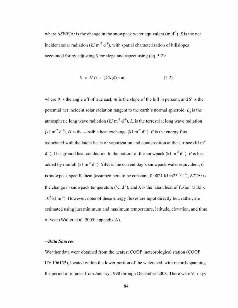
84
where ΔSWE/Δt is the change in the snowpack water equivalent (m d-1), S is the net
incident solar radiation (kJ m-2 d-1), with spatial characterization of hillslopes
accounted for by adjusting S for slope and aspect using (eq. 5.2):
! = !’ (1 + (!"#(!) ∗ !) (5.2)
where ! is the angle off of true east, ! is the slope of the hill in percent, and !’ is the
potential net incident solar radiation tangent to the earth’s normal spheroid. La is the
atmospheric long wave radiation (kJ m-2 d-1), Lt is the terrestrial long wave radiation
(kJ m-2 d-1), H is the sensible heat exchange (kJ m-2 d-1), E is the energy flux
associated with the latent heats of vaporization and condensation at the surface (kJ m-2
d-1), G is ground heat conduction to the bottom of the snowpack (kJ m-2 d-1), P is heat
added by rainfall (kJ m-2 d-1), SWE is the current day’s snowpack water equivalent, C
is snowpack specific heat (assumed here to be constant, 0.0021 kJ m23 oC-1), ΔTs/Δt is
the change in snowpack temperature (oC d-1), and λ is the latent heat of fusion (3.35 x
105 kJ m-3). However, none of these energy fluxes are input directly but, rather, are
estimated using just minimum and maximum temperature, latitude, elevation, and time
of year (Walter et al. 2005; appendix A).
--Data Sources
Weather data were obtained from the nearest COOP meteorological station (COOP
ID: 106152), located within the lower portion of the watershed, with records spanning
the period of interest from January 1990 through December 2008. There were 91 days

85
of missing temperature and precipitation data from 1990-2008. Missing data were
estimated using the SWAT weather generator.
The model was initialized with the most accessible datasets for the watershed; when
multiple datasets were considered equally accessible, we used the most current. The
data sets used were: STATSGO soils dataset (USDA-SCS 1993), a GIS based
coverage distributed with the ArcSWAT modeling system. Temperature and
precipitation were, obtained from the closest COOP station, “Moscow U Of I” (COOP
ID: 106152). The National Elevation Dataset (NED) at 30m cell resolution (Gesch
2007; Gesch et al. 2002) was used for topography and the 2001 Multi-Resolution Land
Characteristics (MRLC) Consortium (MRLC 2011) web interface for land use, also at
30m cell resolution (Homer et al. 2004) (available at: Multi-Resolution Land
Characteristics Consortium (MRLC) Available at: http://www.mrlc.gov/. Accessed
2/6/2011.).
--Study Site
Since the purpose of this study is to demonstrate intra-subbasin spatial distribution of
snow, a watershed where the authors have familiarity with and access to was required.
For this reason, the test watershed selected was located above USGS Paradise Creek
stream gage (ID 13346800), (USGS, 2011. USGS Real-Time Water Data for USGS
13346800 Available at: http://waterdata.usgs.gov/usa/nwis/uv?13346800. Accessed
2/6/2011) adjacent to the University of Idaho, Moscow, ID (Latah County, Moscow

86
West quadrangle, Hydrologic Unit 17060108). Recorded discharge (1978-present)
ranged from 0.001 m3s-1 to 27 m3s-1 and elevations range from 775m to 1327m.
The Paradise Creek watershed has an area of 4573 ha, with approximately 50% of the
watershed classified as Agricultural Land/Row Crops (AGRR), 17% Forest Evergreen
(FRSE), 25% Urban Low/Medium/High density and 7% classified as Range-Brush
(RNGB). Within the basin 49% of the soils are classified as THATUNA silt loam,
29% SOUTHWICK silt loam, 15% VASSAR silt loam, and 7% TANEY silt loam.
There are three slope classes with 34% of the watershed in the range of 0-7% slope,
29% of the watershed in the range of 7-16% slope, and 37% of the watershed greater
than 16% slope. Again, since we were interested in assessing the ability of the model
to capture the spatial distributions of snow within a watershed, and since we wanted to
limit the potential effect of over parameterizing possible by including more subbasins
than necessary, we departed from traditional SWAT initialization procedures, and
initialized a watershed as a single subbasin. This allowed true rendering of the HRU
distribution (e.g., we did not reduce the number of HRUs using the thinning function
in the interface), which resulted in 409 HRUs.
--Model Modifications
We created the new PB snowmelt subroutine (owsnowmelt.f) that solves the daily
energy balance for a snowpack. We modified the version of the Walter et al. (2005)
PB snowmelt routine to include the influences of land use (vegetation), slope, and
aspect on incident solar radiation, S, and changes in elevation within the subbasin. All

87
parameters are derived from data currently required to initialize SWAT. We use the
daily leaf area index (LAI) calculated in SWAT for canopied land classifications at the
hydrologic response unit (HRU) level to adjust solar radiation linearly, where a LAI
above 1 results in S = 0. Aspect, calculated during the digital elevation model (DEM)
processing (using the D8 algorithm of Tarboton, 1997), and slope, are already
determined for each HRU and were used to adjust the solar declination value in the
calculation of S (i.e., Walter et al. 2005), with true East and West facing slopes
considered equivalent to a horizontal plane on the earth’s surface.
The effects of forest canopies on the sensible heat exchange (eq. 5.1, H), latent heats
of vaporization and condensation at the surface (E), and atmospheric long wave
radiation (La), were included in SWAT-PB by adjusting the mean wind velocity below
forest canopies to 50% of the model supplied wind velocity (Ohta et al., 1999; Oliver,
1971), which reduced eq. 5.1, H and E values accordingly (Walter et al. 2005). In
areas of the watershed dominated by evergreen land cover, we assume that long wave
radiation from the canopy is much greater than from the atmosphere and the
atmospheric long wave radiation La was calculated with the Stefan-Botzman equation
using the average canopy temperature and an emissivity equal to the LAI for LAI<1
and equal to one for LAI≥1.
Critical for the solution of eq. 5.1 are accurate estimates of temperature and
precipitation throughout the watershed, both of which can vary spatially due to
subbasin topology. Lapse rates, for both temperature and precipitation, were added

88
using published values of 10oC/km elevation and 770mm/km elevation, respectively
(Bigler et al., 2007; Ahl et al., 2008). Different values may be appropriate in different
locations, but these values are either known or can be easily determined, and are often
regionally representative. To minimize SWAT code modifications, the temperature
and precipitation lapse rates were only included in the new snowmelt routine.
Because the new snowmelt model only required a single new subroutine,
owsnowmelt.f, (to replace the current SWAT snowmelt routine, snom.f), only one line
of code was modified in the existing surface.f routine, i.e., the line calls the new
snowmelt routine instead of the old one. Several variables (surface albedo, snow
depth, and snow temperature) had to be tracked through the model run, so two lines in
the modparm.f module and four lines to the allocate.f subroutine had to be modified.
We also modified the code to permit frozen soil seepage by commenting out the
logical test for frozen soil in percmicro.f (from Easton et al. 2008). Finally, the soils
were reclassified to include topographic aspects and relative elevation in the watershed
into four increments varying from 100m to 400m, with more extreme sloping areas
having larger increments; the latter is similar to the method introduced by Easton et al.
(2008) for including variable source areas in SWAT using a soil topographic index
(STI), although here we integrate elevation ranges as opposed to ranges of STI.
--Calibration
The watershed was calibrated for both SWAT-TI and SWAT-PB versions using the
Differential Evolution Optimization library (DEoptim) (Ardia and Mullen, 2009)

89
within the statistical computing environment R (Ihaka and Gentleman, 1996; RDC
Team, 2009). Each of the SWAT2005 parameters (defined in Table 5.1) was defined
as either those calibrated by replacement within an initial range published in the
literature (Table 5.1, Method column as ”replace”) or those calibrated by adjusting the
base initialization default variables by a certain percentage (Table 5.1, Method column
as ”percent”). We performed 15 calibrations for 15 individual years within the 1994-
2008 period for both SWAT-TI and SWAT-PB. This was done to demonstrate the
ability of each model in basins with limited historical data. Ideally we would calibrate
each process independently, but this is not the way it is usually done because often we
only have discharge data at the watershed outlet and without specific snow data it is
infeasible to calibrate the snow model independently of the rest of the hydrological
model. It should be noted that calibration of the parameters SFTMP, SMTMP,
SMFMX, SMFMN, TIMP was only required for SWAT-TI since SWAT-PB requires
no calibration for snow modeling. Soil parameters (Depth, BD, AWC, KSAT), are
examples of those in which defaults are perturbed with the DEoptim algorithm to find
an optimal calibration. The curve number (CN) and variables controlling ground water
(GW_DELAY, ALPHA_BF, QWQMN), and surface and lateral flow parameters
(SURLAG, LAT_TTIME), which often change depending on subbasin characteristics,
are examples of those in which we set a range from published values and let the
DEoptim algorithm hunt for the best result. The local-to-best differential evolution
strategy (Price et al. 2005) was used for both the range calibrated and perturbed
parameters, with daily predicted vs observed flow Nash Sutcliffe efficiencies (NSE)
(Nash and Sutcliffe, 1970) used as the objective function.

90
Table 5.1. Calibrated parameters used for Differential Evolution Optimization. SFTMP, SMTMP, SMFMX, SMFMN, TIMP being calibrated only for the TI version of SWAT.
Variable Definition Method Range/Percent SFTMP Snowfall temperature [C] replace -5 – 5 Deg. C SMTMP Snow melt base temperature [C] replace -5 – 5 Deg. C SMFMX Melt factor for snow on June 21 [mm H2O/C-day] replace -5 – 5 Deg. C SMFMN Melt factor for snow on December 21 [mm H2O/C-
day]
replace -5 – 5 Deg. C TIMP Snow pack temperature lag factor replace -5 – 5 Deg. C GW_DELAY Groundwater delay [days] replace 1 - 180 Days ALPHA_BF Baseflow alpha factor [days] replace 1 - 180 Days SURLAG Surface runoff lag time [days] replace 1 - 180 Days GWQMN Threshold depth of water in the shallow aquifer [mm] replace 1 - 200 mm LAT_TTIME Lateral flow travel time [days] replace 1 - 180 Days ESCO Soil evaporation compensation factor replace .2 - .99 CN2 Initial SCS CN II value replace 65 - 85 Depth Soil layer depths [mm] percent 50 – 150 % BD Bulk Density Moist [g/cc] percent 50 – 150 % AWC Average available water [mm/mm] percent 50 – 150 % KSAT Saturated conductivity [mm/hr] percent 50 – 150 %

91
--Corroboration Methods
Since there are very few spatially distributed snow depth sensors in the study site,
corroboration was accomplished with a combination of methods including evaluating
the models ability to predict daily discharge at the watershed outlet, comparing the
modeled SWE to the nearest active SNOTEL station, visual corroboration against
LandSat imagery, and analytical comparison of spatial depth with LandSat pixel
brightness.
Corroboration of the calibrated models at the outlet was performed by running the best
single year calibration for each model from 1990-2008 period, and comparing
measured against daily simulated basin outflow for the period of 1994-2008. 1990 –
1993 was used as the warm-up period for which the model is allowed to reach
numerical equilibrium.
Data from the SNOTEL station located above the highest point of the Paradise Cr.
Drainage (1327m) was compared to the closest HRU elevation increment within the
modeled basin. SNOTEL Site 989 (USGS, 2010. Moscow Mountain (989) - Site
Information and Reports. Available at:
http://www.wcc.nrcs.usda.gov/nwcc/site?sitenum=989&state=id. Accessed
9/20/2010.), Moscow Mountain in Latah county ID, at 1433m has reported since the
beginning of the snow year 2000. Though the station only has records for the last 8
years of the study period and is approximately 100m above the highest point in the
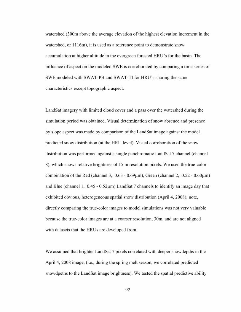
92
watershed (300m above the average elevation of the highest elevation increment in the
watershed, or 1116m), it is used as a reference point to demonstrate snow
accumulation at higher altitude in the evergreen forested HRU’s for the basin. The
influence of aspect on the modeled SWE is corroborated by comparing a time series of
SWE modeled with SWAT-PB and SWAT-TI for HRU’s sharing the same
characteristics except topographic aspect.
LandSat imagery with limited cloud cover and a pass over the watershed during the
simulation period was obtained. Visual determination of snow absence and presence
by slope aspect was made by comparison of the LandSat image against the model
predicted snow distribution (at the HRU level). Visual corroboration of the snow
distribution was performed against a single panchromatic LandSat 7 channel (channel
8), which shows relative brightness of 15 m resolution pixels. We used the true-color
combination of the Red (channel 3, 0.63 - 0.69µm), Green (channel 2, 0.52 - 0.60µm)
and Blue (channel 1, 0.45 - 0.52µm) LandSat 7 channels to identify an image day that
exhibited obvious, heterogeneous spatial snow distribution (April 4, 2008); note,
directly comparing the true-color images to model simulations was not very valuable
because the true-color images are at a coarser resolution, 30m, and are not aligned
with datasets that the HRUs are developed from.
We assumed that brighter LandSat 7 pixels correlated with deeper snowdepths in the
April 4, 2008 image, (i.e., during the spring melt season, we correlated predicted
snowdpeths to the LandSat image brightness). We tested the spatial predictive ability
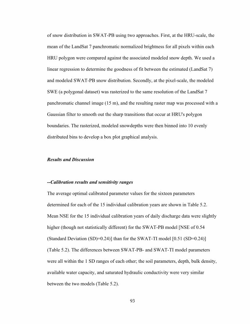
93
of snow distribution in SWAT-PB using two approaches. First, at the HRU-scale, the
mean of the LandSat 7 panchromatic normalized brightness for all pixels within each
HRU polygon were compared against the associated modeled snow depth. We used a
linear regression to determine the goodness of fit between the estimated (LandSat 7)
and modeled SWAT-PB snow distribution. Secondly, at the pixel-scale, the modeled
SWE (a polygonal dataset) was rasterized to the same resolution of the LandSat 7
panchromatic channel image (15 m), and the resulting raster map was processed with a
Gaussian filter to smooth out the sharp transitions that occur at HRU's polygon
boundaries. The rasterized, modeled snowdepths were then binned into 10 evenly
distributed bins to develop a box plot graphical analysis.
Results and Discussion
--Calibration results and sensitivity ranges
The average optimal calibrated parameter values for the sixteen parameters
determined for each of the 15 individual calibration years are shown in Table 5.2.
Mean NSE for the 15 individual calibration years of daily discharge data were slightly
higher (though not statistically different) for the SWAT-PB model [NSE of 0.54
(Standard Deviation (SD)=0.24)] than for the SWAT-TI model [0.51 (SD=0.24)]
(Table 5.2). The differences between SWAT-PB- and SWAT-TI model parameters
were all within the 1 SD ranges of each other; the soil parameters, depth, bulk density,
available water capacity, and saturated hydraulic conductivity were very similar
between the two models (Table 5.2).
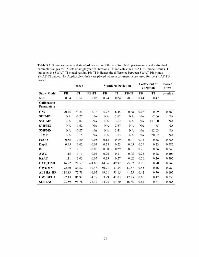
94
Table 5.2. Summary mean and standard deviation of the resulting NSE performance and individual parameter ranges for 15 sets of single year calibrations. PB indicates the SWAT-PB model results, TI indicates the SWAT-TI model results, PB-TI indicates the difference between SWAT-PB minus SWAT-TI values. Not Applicable (NA’s) are placed where a parameter is not used for the SWAT-PB model.
Mean Standard Deviation Coefficient of Variation
Paired t-test
Snow Model PB TI PB-TI PB TI PB-TI PB TI p-value NSE 0.54 0.51 0.03 0.24 0.24 -0.01 0.44 0.47 Calibration Parameters
CN2 70.45 73.21 -2.76 5.77 6.45 -0.68 0.08 0.09 0.380 SFTMP NA -1.27 NA NA 2.62 NA NA -2.06 NA SMTMP NA 0.02 NA NA 3.62 NA NA 181.00 NA SMFMX NA -1.62 NA NA 2.67 NA NA -1.65 NA SMFMN NA -0.27 NA NA 3.41 NA NA -12.63 NA TIMP NA 0.15 NA NA 3.13 NA NA 20.87 NA ESCO 0.55 0.50 0.05 0.18 0.19 -0.01 0.33 0.38 0.885 Depth 0.95 1.02 -0.07 0.28 0.23 0.05 0.29 0.23 0.582 BD
1.07 1.13 -0.06 0.30 0.29 0.01 0.28 0.26 0.240 AWC 1.15 1.11 0.04 0.26 0.31 -0.05 0.23 0.28 0.406 KSAT 1.11 1.05 0.05 0.29 0.27 0.02 0.26 0.26 0.495 LAT_TIME 46.92 71.57 -24.65 44.86 49.92 -5.07 0.96 0.70 0.869 GWQMN 92.30 81.82 10.48 50.71 37.34 13.37 0.55 0.46 0.980 ALPHA_BF 118.83 72.78 46.05 49.61 51.15 -1.55 0.42 0.70 0.197 GW_DELA
Y
82.13 86.92 -4.79 53.29 41.03 12.25 0.65 0.47 0.253 SURLAG 73.59 96.76 -23.17 44.95 61.80 -16.85 0.61 0.64 0.585

95
Interestingly, the variability in the calibrated parameters values over the 15 year-by-
year calibrations was similar between the two models as shown with a paired t-test
grouped by calibration, with the exception of the snow parameters, SFMP, SMTMP,
SMFMX, and SMFMN, which needed no calibration in SWAT-PB (see coefficients of
variation in Table 5.2). For SWAT-TI, the variability in the calibrated snow
parameters was one to four orders of magnitude greater than any of the other
parameters (Table 5.2).
--Stream discharge corroboration
After determining the optimal calibrated values (based on stream discharge) for all
parameters and both models for each of 15 individual years, each specific calibration
parameter set was run and compared to measured daily stream flow for the entire
range of years 1994-2008. In general, SWAT-PB performed substantially better than
SWAT-TI, mean NSE of 0.45 and 0.32, respectively (Table 5.3). However, the best
NSE for SWAT-TI, 0.60, was slightly higher than the best SWAT-PB run, 0.58 (Table
5.3). Though not statistically different, the differences between the models were much
greater for the poorer performing simulation; the lowest NSE for the SWAT-TI was -
0.11 was substantially lower than the worst SWAT-PB run, NSE=0.18.
--Snow depth corroboration
Figure 5.1 compares the SWAT predicted SWE for water years 2001-2008 using
parameters from the best calibration-year for SWAT-TI and SWAT-PB (1997 and
2003, respectively) and SNOTEL measure SWE (note that the SNOTEL station is

96
Table 5.3. Corroboration Results, summary of the 15 yearly calibrations corroborated against stream flow from 1994-2008
PB TI Mean NSE 0.42 0.32 Max NSE 0.58 0.60 Min NSE 0.25 -0.11 SD NSE 0.10 0.18
.

97
Figure 5.1. SWE for HRU 185, An evergreen forest at the highest elevation in the watershed for water years 2001 - 2008. Blue dotted line is SNOTEL measured, 300m above the average elevation of the highest elevation increment in the watershed, dashed brown line is BP, and orange line is optimal calibration for TI.
2001 2002 2003 2004
0400
800
SWE(mm)
SWE(mm)
SNOTELSWAT_PBSWAT_TI
2005 2006 2007 2008
0200
400
SWE(mm)
SWE(mm) SNOTEL
SWAT_PBSWAT_TI

98
100m above the watershed). In Fig. 5.1 it is evident that the optimum calibration of the
SWAT-TI model resulted in almost no snow accumulation over this period. This
highlights the importance of recognizing that a model’s capacity to reproduce flow at
the outlet, i.e., the data used to optimize the calibration, does not imply that the
internal processes or spatial patterns are correctly simulated. Here, the calibration of
SWAT-TI produced parameter values for the groundwater and runoff processes that
gave better agreement between modeled and measured stream flow than could be
achieved via snow accumulation and melt; note, there were too many parameter
combinations to determine precisely which parameter values off-set the lack of
modeled snow accumulation. As is expected, because calibration is unnecessary, the
PB-model accumulates and melts snow, no matter what the outcome of
autocalibration. In Fig. 5.1, as expected, the timing of the annual accumulation and
melt cycles for the PB-model coincide well with the measured snow accumulation and
melt measured at the SNOTEL gauge but the magnitude of snow accumulation is
lower because the highest HRU is below the SNOTEL, i.e., we expect more snow
accumulation at higher elevations.
--Corroboration of the spatial distribution of snow
In Fig. 5.2, we visually compare the snow visible within the LandSat 7 scene from
April 4, 2008 (Fig. 5.2a) with the predicted snow depth for both SWAT-PB (Fig. 5.2b)
and SWAT-TI (Fig. 5.2c). Strips of missing data present in Fig. 5.2a are a result of the
May 2003 Scan Line Corrector failure in the ETM+ instrument. While this represents
only a single day during the 10 year model run it represents some of the only

99
Figure 5.2. Spatial corroboration using LandSat 7 imagery from April 3, 2008 with oval highlighting the same area in each scene. Upper left frame(a) LandSat 7 distinctly shows hillslope snow distribution. Upper right frame(b), SWAT-PB distinctly shows linear features of hillside snow that align with the LandSat 7 imagery. Lower left (c) SWAT-TI shows relatively uniform snow distribution.
Ü SWE(mm)
0
1 - 128
129 - 179
180 - 189
190 - 202
203 - 232
233 - 320
321 - 407
408 - 463
464 - 489
a
c
b

100
available, high resolution spatial data, and it is difficult to find scenes that are capable
of distinguishing the influence of aspect on snow distribution. Figure 5.2c shows the
snow depth for the entire subbasin in the SWAT-TI model, and it is clear that there is
little snow, and that it does not vary spatially, using the optimal calibration run for
SWAT-TI (calibration year 1997). In Fig. 5.2c there are no significant differences in
SWAT-TI predicted snow depth among land uses, slopes, and aspects. SWAT-PB
results (Fig. 5.2b) show a more realistic distribution of snowpack with differences in
snow depth on north- verses south-facing slopes and, as expected, more snow at higher
elevations and in the evergreen forest (Fig. 5.2b). The elevation effects are abrupt due
to the way elevation was incremented into four elevation groups, but increasing the
number of elevation groups in the initialization would result in a more continuous and
gradual increase in snow depth with elevation.
Figure 5.3 confirms SWAT-PB’s ability to predict the impact of aspect on snow
distribution throughout a snow year. In this comparison, we grouped all HRUs that
had the same elevation, slope, land use, and soils, with the differentiating factor being
the direction the slope is facing. This allows a comparison of the influence of aspect in
the model. Cleary shown in Fig. 5.3, is that SWAT-PB maintains snowpack longer
and at a greater depth on north facing slopes than on south facing slopes, which is
intuitive as north facing slopes receive less incident solar radiation, but is none-the-
less ignored in SWAT-TI.
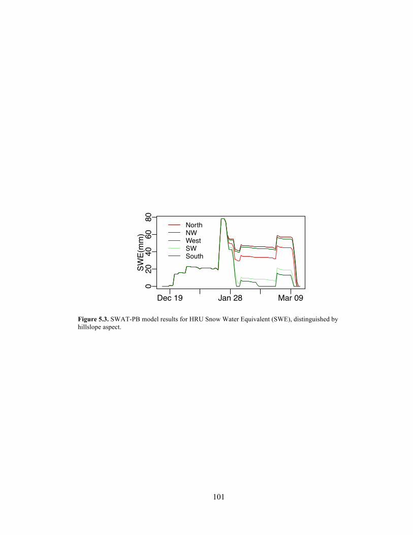
101
Figure 5.3. SWAT-PB model results for HRU Snow Water Equivalent (SWE), distinguished by hillslope aspect.
020
40
60
80
SW
E(m
m)
Dec 19 Jan 28 Mar 09
NorthNWWestSWSouth

102
After visual corroboration of the spatial distribution of snow in the watershed, we
perform an analytical comparison of the SWAT-PB model results against the LandSat
7 imagery. Using the same LandSat 7 scene as was used for the visual comparison, a
linear regression of modeled SWE against the LandSat 7 panchromatic brightness
performed from the perspective of the polygonal HRU data set (Fig. 5.4a)
demonstrates the relationship between mean pixel brightness and SWAT-PB modeled
SWE, and although there is significant variation at values of low SWE/pixel brightness,
SWAT-PB is able to capture the general trend. Figure 5.4b further demonstrates this
relationship from a raster cell perspective, and again is reassuringly able to capture the
expected trend. Figure 5.4 also highlights the complexities of determining snow depth
using remote sensing as variable illumination, detector saturation and other
impediments make determining not only the presence or absence, but also the depth
and SWE of snow complex (Rosenthal and Dozier, 1996).
Summary and Conclusions
This study demonstrates that a simple PB snowmelt model can be incorporated into an
existing operational hydrologic model with little change to the original code base and
without adding substantial input data requirements. On a 46km2 watershed in northern
Idaho, USA, we demonstrate this by incorporating an energy budget, PB snow model
into SWAT2005 using only readily available data, e.g., maximum and minimum daily
temperature, geographic latitude, and published values for physical parameters, e.g.,
latent heat of fusion, snow heat capacity, etc. SWAT2005 actually has the capacity to
directly use many parameters that were estimated in this study; for example solar

103
Figure 5.4. Left(a) HRU-based comparison of SWAT-PB SWE (mm) vs LandSat 7 Channel 8 panchromatic brightness. Mean for each polygon extracted from raster LandSat 7 scene. Right (b) Raster cell based comparison of SWAT-PB SWE(mm) vs LandSat 7 Channel 8 panchromatic brightness with boxplots showing the progression of grouped means and pixel spread.
!
!
!
!
!
!
!
!
!!
!
!
!
!
!
!
!
!
!
!
!
!
!!
60 70 80 90
170
175
180
185
190
195
LandSat Ch. 8 Brightness
SWAT−P
B SW
E. (m
m)
y=0.24x+172.1Residual standard error: 4.66R−squared: 0.2185p−value: 0.02128
a
50 100 150
175
180
185
190
LandSat Ch. 8 Brightness
SWAT−P
B SW
E. (m
m)
50 100 15050 100 150
Mean
b

104
radiation, wind, and humidity and we expect that SWAT-PB would perform better
than demonstrated here if these were used directly when and/or where these data exist.
Because this study was performed using many independent one-year calibrations, we
were able to show the high degree of variability in the calibrated TI parameters from
year to year, emphasizing the need for process-based models when limited or no data
is available (i.e. ungaged basins). For this watershed, it was interesting to discover that
the optimal calibrated parameter set for SWAT-TI actually resulted in simulating no
snow some years, despite direct observations and measurements that show snow
accumulation and melt every year. This indicates that calibrating a TI model against
only watershed outlet discharge may necessarily misrepresent other hydrologic
processes, as the error in one of the most important hydrologic processes can only be
compensated for with induced errors in other processes. Overall, this study affirms
that calibrating hydrological models to watershed outlet discharge may not ensure
internal processes and patterns of water distribution are correctly simulated, that
spatial snowmelt does not require extensive model modification, and that the
complexity of data requirements need not be a hurdle for those processes dependent on
the surface energy budget. Fine resolution distributed snow data in more watersheds
are required to further test the model proposed here. One final note, while we have
focused on snowmelt/accumulation as it relates to the energy budget, we envision
methods such as these to be applicable to a number of different, relevant hydrologic
processes.

105
Supporting Information
Additional Supporting Information may be found in the online version of this article:
owsnowmelt.f, a FORTRAN subroutine written in format, data structure, and
paradigm of SWAT2005 and SWAT2009 source code with minor modification to
surface.f, modparm.f, and allocate.f .
Acknowledgements
LandSat 7 Enhanced Thematic Mapper Plus (ETM+) courtesy of the U.S. Geological
Survey.
This material is based upon work supported by Synthesis and Analysis of 13 CSREES
CEAP Projects and the Cooperative State Research, Education and Extension
Service, US Department of Agriculture, under agreement No. 2007-51130-03992.

106
REFERENCES
Ahl, R.S., Woods, S.W., Zuuring, H.R. 2008. Hydrologic calibration and validation of
SWAT in a snow-dominated rocky mountain watershed, Montana, USA. Journal of
the American Water Resources Association, 44(6):1411-1430.
Ardia, D., Mullen, K. 2009. DEoptim: Differential evolution optimization in R. R
package version 2.0-3. Available at: http://CRAN.R-project.org/package=DEoptim.
Accessed 09/03, 2010.
Arnold, J.G., Gassman, P.W., White, M.J. 2010. New developments in the SWAT
ecohydrology model. In: Proceedings of the Watershed Technology Conference,
February 21-24, American Society of Agricultural and Biological Engineers, Earth
University, Costa Rica.
Arnold, J.G., Srinivasan, R., Muttiah, R.S., Williams, J.R. 1998. Large area hydrologic
modeling and assessment - Part I: Model development. Water Resources Bulletin,
34(1):73-89.
Arnold, J.G., Fohrer, N. 2005. Preface: SWAT2000: Current capabilities and research
opportunities in applied watershed modelling. Hydrological Processes, 19(3):563-572.
Baveye, P., Boast, C.W. 1999. Physical scales and spatial predictability of transport
processes in the environment. Geophysical Monograph, 108:261-280.
Bigler, C., Gavin, D.G., Gunning, C., Veblen, T.T. 2007. Drought induces lagged tree
mortality in a subalpine forest in the Rocky Mountains. Oikos, 116(12):1983-1994.

107
Borah, D.K., Bera, M. 2003. Watershed-scale hydrologic and nonpoint-source
pollution models: Review of mathematical bases. Transactions of the ASABE,
46(6):1553-1566
Dahlke, H.E., Easton, Z.M., Fuka, D.R., Lyon, S., Steenhuis, T.S. 2009. Developing
and testing a semi-distributed model to predict saturated area dynamics in an
agriculturally dominated watershed. Ecohydrology, 2(3): 337-349.
Debele B., Srinivasan R., Gosain A.K. 2010. Comparison of Process-based and
temperature-index snowmelt modeling in SWAT. Water Resources Management,
24(6):1065-1088.
Easton, Z.M., Fuka, D.R., Walter, M.T., Cowan, D.M., Schneiderman, E.M.,
Steenhuis, T.S. 2008. Re-conceptualizing the soil and water assessment tool (SWAT)
model to predict runoff from variable source areas. Journal of Hydrology, 348(3-
4):279-291.
Easton, Z.M., Fuka, D.R., White, E.D, Collick, A.S., Ashagre, B.B, McCartney, M.,
Awulachew, S.B., Ahmed, A.A., Steenhuis, T.S. 2010. A multi basin SWAT model
analysis of runoff and sedimentation in the Blue Nile, Ethiopia. Hydrology and Earth
System Science, 14:1827-1841. doi:10.5194/hess-14-1827-2010, 2010.
Easton, Z.M., Walter, M.T., Fuka, D.R., White, E.D., Steenhuis, T.S. 2011. A simple
concept for calibrating runoff thresholds in quasi-distributed variable source area
watershed models. Hydrological Processes, 25(20):3131-3143, doi:10.1002/hyp.8032,
2011.
Fontaine, T., Cruickshank, T., Arnold, J., Hotchkiss, R. 2002. Development of a
snowfall–snowmelt routine for mountainous terrain for the Soil Water Assessment
Tool (SWAT). Journal of Hydrology, 262(1-4):209-223.

108
Frankenberger, J.R., Brooks, E.S., Walter, M.T., Walter, M.F. 1999. A GIS-based
variable source area hydrology model. Hydrological Processes, 13(6):804-822.
Gassman, R.W., Reyes, M.R., Green, C.H., Arnold, J.G. 2007. The Soil and Water
Assessment Tool: Historical development, applications, and future research directions.
Transactions of the ASABE, 50(4):1211-1250.
Gesch, D.B. 2007. "Chapter 4 – The National Elevation Dataset", in Maune, D.,
ed., Digital Elevation Model Technologies and Applications: The DEM Users Manual,
2nd Edition: American Society for Photogrammetry and Remote Sensing, Bethesda,
Maryland.
Gesch D., Oimoen M., Greenlee S., Nelson C., Steuck M., Tyler D., 2002. The
National Elevation Dataset. Photogrammetric Engineering and Remote Sensing,
68(1):5-11.
van Griensven A., Bauwens, W. 2003. Concepts for river water quality processes for
an integrated river basin modeling. Water Science and Technology, 48(3):1-8.
Homer, C., Huang, C., Yang, L., Wylie, B., Coan, M. 2004. Development of a 2001
national landcover database for the United States. Photogrammetric Engineering and
Remote Sensing, 70:829-840.
Ihaka, R., Gentleman R. 1996. R: A language for data analysis and graphics. Journal
of Computational and Graphical Statistics, 5(3):299-314.
Mirchi, A., Watkins, Jr., D., Madani, K. 2009. “Chapter 6 – Modeling for watershed
planning, management, and decision making”, in: Vaughn J.C., (Eds.), Watersheds:

109
management, restoration, and environmental impact. Nova Science Publishers, New
York. pp. 221-224
Moore, R.D., Thompson, J.C. 1996. Are water table variations in a shallow forest soil
consistent with the TOPMODEL concept? Water Resources Research, 32(3):663-669.
Nash, J.E., Sutcliffe, J.V. 1970. River flow forecasting through conceptual models part
I — A discussion of principles. Journal of Hydrology, 10(3):282-290.
Ohta, T., Suzuki, K., Kodama,Y., Kubota, J., Kominami, Y., Nakai, Y. 1999.
Characteristics of the heat balance above the canopies of evergreen and deciduous
forests during the snowy season. Hydrological Processes, 13(14-15):2383-2294.
Oliver, H. 1971. Wind profiles in and above a forest canopy. Quarterly Journal of the
Royal Meteorological Society, 97(414):548-553.
Pagano T., Garen, D. 2005. A recent increase in western US streamflow variability
and persistence. Journal of Hydrometeorology, 6(2):173-179.
Price K.V., Storn, R.M., Lampinen, J.A. 2005. Differential evolution: A practical
approach to global optimization (Natural Computing Series). Springer-Verlag. Berlin,
Heidelberg.
Ramanarayanan, T., Narasimhan, B., Srinivasan, R. 2005. Characterization of fate and
transport of isoxaflutole, a soil-applied corn herbicide, in surface water using a
watershed model. Journal of Agricultural and Food Chemistry, 53(22):8848-8858.
RDC Team. 2009. R: A Language and Environment for Statistical Computing.
Available: http://www.R-project.org. Accessed 1 January 2010.

110
Rosenthal, W., Dozier, J. 1996. Automated mapping of montane snow cover at
subpixel resolution from the Landsat Thematic Mapper. Water Resources Research,
32(1):115-130.
Santhi, C., Arnold, J.G., Williams, J.R., Dugas, W.A., Srinivasan, R., Hauck L.M.
2001. Validation of the SWAT model on a large river basin with point and nonpoint
sources. Journal of the American Water Resources Association, 37:1169-1188.
Srinivasan, R., Zhang, X., Arnold, J. 2010. SWAT ungauged: Hydrological budget
and crop yield predictions in the upper Mississippi River basin. Transactions of the
ASABE, 53(5):1533-1546.
Steenhuis, T.S., Parlange, J.Y., Sanford, W.E., Heilig, A., Stagnitti, F., Walter, M.F.
1999. Can we distinguish Richards' and Boussinesq's equations for hillslopes?: The
Coweeta experiment revisited. Water Resources Research, 35(2):589-593.
Tarboton, D.G. 1997. A new method for the determination of flow directions and
upslope areas in grid digital elevation models, Water Resources Research, 33(2):309–
319.
U.S. Department of Agriculture, Soil Conservation Service (USDA-SCS). 1993.
STATSGO data users guide. Miscellaneous Publication Number 1492.
Walter, M.T., Parlange, J.Y., Walter, M.F., Xin, X., Scott, C.A. 2001. Modeling
pollutant release from a surface source during rainfall runoff. Journal of
Environmental Quality, 30(1):151–159
Walter, M.T., Brooks, E.S., McCool, D.K., King, L.G., Molnau, M., Boll, J. 2005.
Process-based snowmelt modeling: does it require more input data than temperature-
index modeling? Journal of Hydrology, 300(1-4):65-75.

111
White, E.D., Easton, Z.M., Fuka, D.R., Collick, A.S., Adgo, E., McCartney, M.,
Awulachew, S.B., Selassie, Y.G., Steenhuis, T.S. 2011. Development and application
of a physically based landscape water balance in the SWAT model. Hydrological
Processes, 25:915-925. doi:10.1002/hyp.7876, 2011.
Yarnell, S.M., Viers, J.H., Mount, J.F. 2010. Ecology and management of the spring
snowmelt recession. Bioscience, 60(2):114-127.
Zeinivand, H., De Smedt, F. 2009. Hydrological modeling of snow accumulation and
melting on river basin scale. Water Resources Management, 23(11):2271-2287.
Zhang, X., Srinivasan, R., Debele, B., Hao, F. 2008. Runoff simulation of the
headwaters of the Yellow River using the SWAT model with three snowmelt
algorithms. Journal of the American Water Resources Association, 44(1):48-61.

112
APPENDIX A
DATA SOURCES FOR CHAPTER 2
Daily stream flow and CFSR weather data for each basin can be obtained using the
following CRAN distributed EcoHydRology package using the following script where
the stream flow is stored in the “flowgage” list and the CFSR data is stored in the
“weather” dataframe:
# Install and load the libraries install.packages("EcoHydRology") library(EcoHydRology) # Flow and CFSR for Cross River, NY, USA flowgage_id="01374890" flowgage=get_usgs_gage(flowgage_id) weather=get_cfsr_latlon(flowgage$declat,flowgage$declon) # Flow and CFSR for Tesuque Cr. NM, USA flowgage_id="08302500" flowgage=get_usgs_gage(flowgage_id) weather=get_cfsr_latlon(flowgage$declat,flowgage$declon) # Flow and CFSR for Andreas Cr., CA, USA flowgage_id="10259000" flowgage=get_usgs_gage(flowgage_id) weather=get_cfsr_latlon(flowgage$declat,flowgage$declon) # Flow and CFSR for Town Brook NY, USA flowgage_id= "01421618" flowgage=get_usgs_gage(flowgage_id) weather=get_cfsr_latlon(flowgage$declat,flowgage$declon) # CFSR for Gumara, Ethiopia weather=get_cfsr_latlon(11.747042,37.797672) Stream flow for the Gumara is available from the ministry of water resources at: http://www.mowr.gov.et/
Weather station data for the region surrounding the Gumara is available at the
National Meteorology Agency of Ethiopia: http://www.ethiomet.gov.et/

114
APPENDIX C
A FORTRAN SUBROUTINE WRITTEN IN FORMAT, DATA STRUCTURE, AND
PARADIGM OF SWAT2005 AND SWAT2009 SOURCE CODE FOR CHAPTER 5
subroutine owsnowmelt !! ~ ~ ~ PURPOSE ~ ~ ~ !! this subroutine predicts daily snom melt when the average air !! temperature exceeds 0 degrees Celcius !! ~ ~ ~ INCOMING VARIABLES ~ ~ ~ !! name |units |definition !! ~ ~ ~ ~ ~ ~ ~ ~ ~ ~ ~ ~ ~ ~ ~ ~ ~ ~ ~ ~ ~ ~ ~ ~ ~ ~ ~ ~ ~ ~ ~ ~ ~ ~ ~ ~ !! iida |julian date |day being simulated (current julian date) !! ihru |none |HRU number !! precipday |mm H2O |precipitation on the current day in the HRU !! sno_hru(:) |mm H2O |amount of water in snow in HRU on current day !! snoeb(:,:) |mm H2O |snow water content in elevation band on !! |current day !! snotmp(:) |deg C |temperature of snow pack in HRU !! snotmpeb(:,:)|deg C |temperature of snow pack in elevation band !! timp |none |Snow pack temperature lag factor (0-1) !! |1 = no lag (snow pack temp=current day air !! |temp) as the lag factor goes to zero, the !! |snow pack's temperature will be less !! |influenced by the current day's air !! |temperature !! tmpav(:) |deg C |average air temperature on current day for !! |HRU !! tmx(:) |deg C |maximum air temperature on current day for !! tmn(:) |deg C |minimum temperature for the day in HRU !! snam(:) |NA |soil series name, with included D8 and Elevation !! ~ ~ ~ ~ ~ ~ ~ ~ ~ ~ ~ ~ ~ ~ ~ ~ ~ ~ ~ ~ ~ ~ ~ ~ ~ ~ ~ ~ ~ ~ ~ ~ ~ ~ ~ ~ !! ~ ~ ~ OUTGOING VARIABLES ~ ~ ~ !! name |units |definition !! ~ ~ ~ ~ ~ ~ ~ ~ ~ ~ ~ ~ ~ ~ ~ ~ ~ ~ ~ ~ ~ ~ ~ ~ ~ ~ ~ ~ ~ ~ ~ ~ ~ ~ ~ ~ !! hhprecip(:) |mm H2O |precipitation falling during hour in day !! precipday |mm H2O |amount of water in effective precipitation !! |in HRU !! precipdt(:) |mm H2O |precipitation for the time step during day !! sno_hru(:) |mm H2O |amount of water in snow in HRU on current day !! snoeb(:,:) |mm H2O |snow water content in elevation band on !! |current day !! snofall |mm H2O |amount of precipitation falling as freezing !! |rain/snow on day in HRU !! snomlt |mm H2O |amount of water in snow melt for the day in !! |HRU !! snotmp(:) |deg C |temperature of snow pack in HRU !! snotmpeb(:,:)|deg C |temperature of snow pack in elevation band !! ~ ~ ~ ~ ~ ~ ~ ~ ~ ~ ~ ~ ~ ~ ~ ~ ~ ~ ~ ~ ~ ~ ~ ~ ~ ~ ~ ~ ~ ~ ~ ~ ~ ~ ~ ~ !! ~ ~ ~ LOCAL DEFINITIONS ~ ~ ~ !! name |units |definition !! ~ ~ ~ ~ ~ ~ ~ ~ ~ ~ ~ ~ ~ ~ ~ ~ ~ ~ ~ ~ ~ ~ ~ ~ ~ ~ ~ ~ ~ ~ ~ ~ ~ ~ ~ ~ !! albmax |Decimal % |Max Snow Albedo = .95 !! j |none |HRU number !! owtmpav |deg C |average air temperature on current day for !! |HRU adjusted for lapse rate/altitude !! soldec |radians |solar declination !! snc !degree/45 |D8 direction off of east !! snel |1/100m |Elevation change from meteorological station !! 1k30dsw_pot |kJ/m^2 |30 day sum of potential solar radiation !! sw_pot |kJ/m^2 |extraterestrial potential solar radiation !! latrad |radians |latitude of location in radians

115
!! iida_mo_ago |Julien Date |Julien Date - 30 !! at_tr |Decimal % |atmospheric transmisivity !! b_emp |None |emperical fitting coef !! alb |Decimal % |albedo !! alb_decl(:) |Decimal % |albedo at the start when SWE drops below .3m !! albprev(:) |Decimal % |albedo on previous day in hru !! newsno |Decimal % | equiv water depth of new snow fall !! newsno_den |Decimal % |density of the new snow !! sw_netnet |kJ/m^2 |incident short wave !! lw_t |kJ/m^2 |lw_terestrial !! cc |Decimal % |cloud cover !! ea |kJ/m^2 |atmospheric emissivity !! lw_at |kJ/m^2 |atmospheric long wave !! sh |kJ/m^2 |sensible heat exchange !! heat_resist |day/m |resistance to heat transfer possibly using !! |http://rredc.nrel.gov/wind/pubs/atlas/maps.html#2-7 !! | as a reference for wind speed !! ~ ~ ~ ~ ~ ~ ~ ~ ~ ~ ~ ~ ~ ~ ~ ~ ~ ~ ~ ~ ~ ~ ~ ~ ~ ~ ~ ~ ~ ~ ~ ~ ~ ~ ~ ~ !! Note: For simplification against published methodology, Radiation budjet is !! calculated in kJ/m^2 and multiplied by 1000 to give units of mm. !! ~ ~ ~ ~ ~ ~ END SPECIFICATIONS ~ ~ ~ ~ ~ ~ use parm implicit none real, parameter :: PI=3.141592653589793D0 integer :: j,ii,iida_mo_ago,snc,snel real :: swconst,slope_dec real :: snowdens,newsno_den,latrad, soldec,heat_resist real :: lw_at,alb,sw_net,lw_t,cc,ea,sh,prevsnotmp,rho_s real :: k_month_sw_pot,b_emp,at_tr,sw_pot,rho_a,ef,gh,ph,swecdt real :: del_swe,owtmpav,albmax,ulocal !! initialize local variables j = 0 j = ihru albmax=.95 !! !! Read the D8 aspect, HRU aspect (snc) and elevation (snel) from the soil name. !! Currently, we imbed these characteristics in the soil layer as we wish not to !! alter the base SWAT modeling system. !! read(snam(j),'(2I1)') snc,snel !! Temperature Lapse Rate !! Watch out here, currently the lapse rate is set to .5*snel, due to a our !! setting of 1=100m. In the future we neeed to make this set from input lapse rates. !! owtmpav=tmpav(j) - real(snel)*1.60 !! Calculate snow fall !! Currently the ppt lapse rate is set to 1+.3*snel, due to a 60% rate change from bottom !! to top of example watershed. In the future we can set from the input lapse rate. !! (Bigler, 2007; Ahl, 2008) if (owtmpav <= 0.0) then sno_hru(j) = sno_hru(j)+precipday*(1.0 +real(snel)*0.2) snofall = precipday *(1.0 +real(snel)*0.2) precipday = 0. hhprecip(:) = 0. precipdt(:) = 0. else snofall = 0.0 endif !! !! Solutions from here to Balance see Walter et al. 2005 !! unless otherwise noted. !! !! Solar Radiation !! swconst=117.5e3 if (sub_lat(hru_sub(j)) < 1.e-4) sub_lat(hru_sub(j)) = & & wlat(hru_sub(j)) latrad = sub_lat(hru_sub(j)) / 57.296 iida_mo_ago=iida-30

116
if (iida_mo_ago<0) iida_mo_ago=365+iida_mo_ago soldec=.4102*sin(2*3.1416/365*(iida_mo_ago-80)) k_month_sw_pot=swconst/3.1416*(acos(-tan(soldec)*tan(latrad))* & & sin(latrad)*sin(soldec) + cos(latrad)*cos(soldec)* & & sin(acos(-tan(soldec)*tan(latrad))))/1000.0 slope_dec=-SIN((real(snc)-1.0)*PI*2.0/8.0)*hru_slp(j) soldec=.4102*sin(2*3.1416/365*(iida-80)) + slope_dec if((soldec+latrad)>(PI/2.).or.(-tan(soldec)*tan(latrad)).ge.1.0) & & then sw_pot=0.0 else sw_pot=swconst/3.1416*(acos(-tan(soldec)*tan(latrad))* & & sin(latrad)*sin(soldec) + cos(latrad)*cos(soldec)* & & sin(acos(-tan(soldec)*tan(latrad)))) endif if (iida .ge. 83 .and. iida .le. 263) then b_emp=.282*latrad**(-.431) else b_emp=.170*latrad**(-.979) endif at_tr=.75*(1-exp(-b_emp/k_month_sw_pot*(tmx(j)-tmn(j))**2)) if(alb_decl(j)<=.01)alb_decl(j)=.8 if(albprev(j)<=.01)albprev(j)=.8 snowdens=.4 if (snofall .gt. 0.0) then newsno_den=50.+3.4*(owtmpav+15.) alb=.95-(.95-albprev(j))*exp(-(4.0*snofall/ & newsno_den/.12)) alb_decl(j)=alb sno_decl(j)=sno_hru(j) elseif (sno_hru(j)< 300.) then if(sno_decl(j) .gt. 0.0 .and. sno_hru(j).gt.0.0) then alb=alb_decl(j)-(alb_decl(j)-.25)*(sno_decl(j)-sno_hru(j))/ & & sno_decl(j) else alb=.25 endif else alb=.35-(.35-.95)*exp(-1.0*(.177+ (alog((.95-.35) / & & (albprev(j)-.35)))**2.16)**.46) alb_decl(j)=alb sno_decl(j)=sno_hru(j) endif albprev(j)=alb sw_net=(1.0-alb)*at_tr*sw_pot*(1.0-min(laiday(j),1.0)) !! !! Long Wave Radiation, Terrestrial !! !! ERROR IN PAPER stefan boltsman constan lw_t=.97*4.9e-6*(owtmpav+273.)**4 !! !! Long Wave Radiation, Atmospheric !! cc=(1.0-at_tr/.75) if(idplt(1,1,ihru).eq.8) then ea=.9 else ea=MAX(0.0000092*(owtmpav+273)**2,(0.0000092*(owtmpav+273)**2 & +0.005*owtmpav)*(1-0.84*cc)+0.84*cc) endif lw_at=ea*4.9e-6*(owtmpav+273.)**4 !! !! Heat from convective vapor exchange. !! for tree canopies, we set u=20%*u per {{52 Ohta, T. 1999;}} {{54 Oliver, HR 1971;}}.

117
!! if(idplt(1,1,ihru).eq.8) then ulocal=.50*u10(j) else ulocal=u10(j) endif heat_resist=.0044578/ulocal sh=-1.29*(snotmp(j)-owtmpav)/heat_resist !! !! Estimate snow pack temperature !! prevsnotmp= snotmp(j) snotmp(j) = snotmp(j) * (1. - timp) + owtmpav * timp if (snotmp(j) >0.0)snotmp=0.0 rho_s= exp((16.78*snotmp(j)-116.8)/(snotmp(j)+273.3))/((273.15+ & & snotmp(j))*.4615) rho_a= exp((16.78*owtmpav-116.8)/(owtmpav+273.3))/((273.15+ & & owtmpav)*.4615) ef=2500*(rho_s-rho_a) / heat_resist !! !! Ground heat conduction. !! gh=173.0 !! !! Precipitation heat. !! ph=0.0 if (owtmpav >= 0.0 ) then ph=4.2E3*owtmpav*precipday/1000.0 endif !! !! Stored Snowpack Energy !! swecdt= 2.1*(snotmp(j)-prevsnotmp)*sno_hru(j)/1000.0 !! !! Balance !! del_swe=1.0/3.35E5*(sw_net+lw_at-lw_t+sh-ef+gh+ph-swecdt) if (del_swe < 0.) del_swe = 0. if (del_swe*1000.0 > sno_hru(j)) del_swe = sno_hru(j)/1000.0 sno_hru(j)= sno_hru(j) - del_swe*1000.0 snomlt=del_swe*1000.0 ! This addition to precipday is post precipday being set to 0.0 due to ! snowfall. This allows melt to runoff even if snow was accumilated ! precipday = precipday + del_swe*1000.0 if (precipday < 0.) precipday = 0. if (nstep > 0) then do ii = 1, 24 hhprecip(ii) = hhprecip(ii) + del_swe/ 24 end do do ii = 1, nstep precipdt(ii+1) = precipdt(ii+1) + del_swe / nstep end do end if snoeb(:,j)=sno_hru(j) snotmpeb(:,j)=snotmp(j) 5000 format(a10,i4,22(a8,1x,e10.3)) 5001 format(a10,i4,i4,22(a8,1x,e10.3)) return end

114
APPENDIX C
A FORTRAN SUBROUTINE WRITTEN IN FORMAT, DATA STRUCTURE, AND
PARADIGM OF SWAT2005 AND SWAT2009 SOURCE CODE FOR CHAPTER 5
subroutine owsnowmelt !! ~ ~ ~ PURPOSE ~ ~ ~ !! this subroutine predicts daily snom melt when the average air !! temperature exceeds 0 degrees Celcius !! ~ ~ ~ INCOMING VARIABLES ~ ~ ~ !! name |units |definition !! ~ ~ ~ ~ ~ ~ ~ ~ ~ ~ ~ ~ ~ ~ ~ ~ ~ ~ ~ ~ ~ ~ ~ ~ ~ ~ ~ ~ ~ ~ ~ ~ ~ ~ ~ ~ !! iida |julian date |day being simulated (current julian date) !! ihru |none |HRU number !! precipday |mm H2O |precipitation on the current day in the HRU !! sno_hru(:) |mm H2O |amount of water in snow in HRU on current day !! snoeb(:,:) |mm H2O |snow water content in elevation band on !! |current day !! snotmp(:) |deg C |temperature of snow pack in HRU !! snotmpeb(:,:)|deg C |temperature of snow pack in elevation band !! timp |none |Snow pack temperature lag factor (0-1) !! |1 = no lag (snow pack temp=current day air !! |temp) as the lag factor goes to zero, the !! |snow pack's temperature will be less !! |influenced by the current day's air !! |temperature !! tmpav(:) |deg C |average air temperature on current day for !! |HRU !! tmx(:) |deg C |maximum air temperature on current day for !! tmn(:) |deg C |minimum temperature for the day in HRU !! snam(:) |NA |soil series name, with included D8 and Elevation !! ~ ~ ~ ~ ~ ~ ~ ~ ~ ~ ~ ~ ~ ~ ~ ~ ~ ~ ~ ~ ~ ~ ~ ~ ~ ~ ~ ~ ~ ~ ~ ~ ~ ~ ~ ~ !! ~ ~ ~ OUTGOING VARIABLES ~ ~ ~ !! name |units |definition !! ~ ~ ~ ~ ~ ~ ~ ~ ~ ~ ~ ~ ~ ~ ~ ~ ~ ~ ~ ~ ~ ~ ~ ~ ~ ~ ~ ~ ~ ~ ~ ~ ~ ~ ~ ~ !! hhprecip(:) |mm H2O |precipitation falling during hour in day !! precipday |mm H2O |amount of water in effective precipitation !! |in HRU !! precipdt(:) |mm H2O |precipitation for the time step during day !! sno_hru(:) |mm H2O |amount of water in snow in HRU on current day !! snoeb(:,:) |mm H2O |snow water content in elevation band on !! |current day !! snofall |mm H2O |amount of precipitation falling as freezing !! |rain/snow on day in HRU !! snomlt |mm H2O |amount of water in snow melt for the day in !! |HRU !! snotmp(:) |deg C |temperature of snow pack in HRU !! snotmpeb(:,:)|deg C |temperature of snow pack in elevation band !! ~ ~ ~ ~ ~ ~ ~ ~ ~ ~ ~ ~ ~ ~ ~ ~ ~ ~ ~ ~ ~ ~ ~ ~ ~ ~ ~ ~ ~ ~ ~ ~ ~ ~ ~ ~ !! ~ ~ ~ LOCAL DEFINITIONS ~ ~ ~ !! name |units |definition !! ~ ~ ~ ~ ~ ~ ~ ~ ~ ~ ~ ~ ~ ~ ~ ~ ~ ~ ~ ~ ~ ~ ~ ~ ~ ~ ~ ~ ~ ~ ~ ~ ~ ~ ~ ~ !! albmax |Decimal % |Max Snow Albedo = .95 !! j |none |HRU number !! owtmpav |deg C |average air temperature on current day for !! |HRU adjusted for lapse rate/altitude !! soldec |radians |solar declination !! snc !degree/45 |D8 direction off of east !! snel |1/100m |Elevation change from meteorological station !! 1k30dsw_pot |kJ/m^2 |30 day sum of potential solar radiation !! sw_pot |kJ/m^2 |extraterestrial potential solar radiation !! latrad |radians |latitude of location in radians

115
!! iida_mo_ago |Julien Date |Julien Date - 30 !! at_tr |Decimal % |atmospheric transmisivity !! b_emp |None |emperical fitting coef !! alb |Decimal % |albedo !! alb_decl(:) |Decimal % |albedo at the start when SWE drops below .3m !! albprev(:) |Decimal % |albedo on previous day in hru !! newsno |Decimal % | equiv water depth of new snow fall !! newsno_den |Decimal % |density of the new snow !! sw_netnet |kJ/m^2 |incident short wave !! lw_t |kJ/m^2 |lw_terestrial !! cc |Decimal % |cloud cover !! ea |kJ/m^2 |atmospheric emissivity !! lw_at |kJ/m^2 |atmospheric long wave !! sh |kJ/m^2 |sensible heat exchange !! heat_resist |day/m |resistance to heat transfer possibly using !! |http://rredc.nrel.gov/wind/pubs/atlas/maps.html#2-7 !! | as a reference for wind speed !! ~ ~ ~ ~ ~ ~ ~ ~ ~ ~ ~ ~ ~ ~ ~ ~ ~ ~ ~ ~ ~ ~ ~ ~ ~ ~ ~ ~ ~ ~ ~ ~ ~ ~ ~ ~ !! Note: For simplification against published methodology, Radiation budjet is !! calculated in kJ/m^2 and multiplied by 1000 to give units of mm. !! ~ ~ ~ ~ ~ ~ END SPECIFICATIONS ~ ~ ~ ~ ~ ~ use parm implicit none real, parameter :: PI=3.141592653589793D0 integer :: j,ii,iida_mo_ago,snc,snel real :: swconst,slope_dec real :: snowdens,newsno_den,latrad, soldec,heat_resist real :: lw_at,alb,sw_net,lw_t,cc,ea,sh,prevsnotmp,rho_s real :: k_month_sw_pot,b_emp,at_tr,sw_pot,rho_a,ef,gh,ph,swecdt real :: del_swe,owtmpav,albmax,ulocal !! initialize local variables j = 0 j = ihru albmax=.95 !! !! Read the D8 aspect, HRU aspect (snc) and elevation (snel) from the soil name. !! Currently, we imbed these characteristics in the soil layer as we wish not to !! alter the base SWAT modeling system. !! read(snam(j),'(2I1)') snc,snel !! Temperature Lapse Rate !! Watch out here, currently the lapse rate is set to .5*snel, due to a our !! setting of 1=100m. In the future we neeed to make this set from input lapse rates. !! owtmpav=tmpav(j) - real(snel)*1.60 !! Calculate snow fall !! Currently the ppt lapse rate is set to 1+.3*snel, due to a 60% rate change from bottom !! to top of example watershed. In the future we can set from the input lapse rate. !! (Bigler, 2007; Ahl, 2008) if (owtmpav <= 0.0) then sno_hru(j) = sno_hru(j)+precipday*(1.0 +real(snel)*0.2) snofall = precipday *(1.0 +real(snel)*0.2) precipday = 0. hhprecip(:) = 0. precipdt(:) = 0. else snofall = 0.0 endif !! !! Solutions from here to Balance see Walter et al. 2005 !! unless otherwise noted. !! !! Solar Radiation !! swconst=117.5e3 if (sub_lat(hru_sub(j)) < 1.e-4) sub_lat(hru_sub(j)) = & & wlat(hru_sub(j)) latrad = sub_lat(hru_sub(j)) / 57.296 iida_mo_ago=iida-30
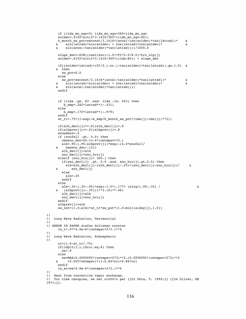
116
if (iida_mo_ago<0) iida_mo_ago=365+iida_mo_ago soldec=.4102*sin(2*3.1416/365*(iida_mo_ago-80)) k_month_sw_pot=swconst/3.1416*(acos(-tan(soldec)*tan(latrad))* & & sin(latrad)*sin(soldec) + cos(latrad)*cos(soldec)* & & sin(acos(-tan(soldec)*tan(latrad))))/1000.0 slope_dec=-SIN((real(snc)-1.0)*PI*2.0/8.0)*hru_slp(j) soldec=.4102*sin(2*3.1416/365*(iida-80)) + slope_dec if((soldec+latrad)>(PI/2.).or.(-tan(soldec)*tan(latrad)).ge.1.0) & & then sw_pot=0.0 else sw_pot=swconst/3.1416*(acos(-tan(soldec)*tan(latrad))* & & sin(latrad)*sin(soldec) + cos(latrad)*cos(soldec)* & & sin(acos(-tan(soldec)*tan(latrad)))) endif if (iida .ge. 83 .and. iida .le. 263) then b_emp=.282*latrad**(-.431) else b_emp=.170*latrad**(-.979) endif at_tr=.75*(1-exp(-b_emp/k_month_sw_pot*(tmx(j)-tmn(j))**2)) if(alb_decl(j)<=.01)alb_decl(j)=.8 if(albprev(j)<=.01)albprev(j)=.8 snowdens=.4 if (snofall .gt. 0.0) then newsno_den=50.+3.4*(owtmpav+15.) alb=.95-(.95-albprev(j))*exp(-(4.0*snofall/ & newsno_den/.12)) alb_decl(j)=alb sno_decl(j)=sno_hru(j) elseif (sno_hru(j)< 300.) then if(sno_decl(j) .gt. 0.0 .and. sno_hru(j).gt.0.0) then alb=alb_decl(j)-(alb_decl(j)-.25)*(sno_decl(j)-sno_hru(j))/ & & sno_decl(j) else alb=.25 endif else alb=.35-(.35-.95)*exp(-1.0*(.177+ (alog((.95-.35) / & & (albprev(j)-.35)))**2.16)**.46) alb_decl(j)=alb sno_decl(j)=sno_hru(j) endif albprev(j)=alb sw_net=(1.0-alb)*at_tr*sw_pot*(1.0-min(laiday(j),1.0)) !! !! Long Wave Radiation, Terrestrial !! !! ERROR IN PAPER stefan boltsman constan lw_t=.97*4.9e-6*(owtmpav+273.)**4 !! !! Long Wave Radiation, Atmospheric !! cc=(1.0-at_tr/.75) if(idplt(1,1,ihru).eq.8) then ea=.9 else ea=MAX(0.0000092*(owtmpav+273)**2,(0.0000092*(owtmpav+273)**2 & +0.005*owtmpav)*(1-0.84*cc)+0.84*cc) endif lw_at=ea*4.9e-6*(owtmpav+273.)**4 !! !! Heat from convective vapor exchange. !! for tree canopies, we set u=20%*u per {{52 Ohta, T. 1999;}} {{54 Oliver, HR 1971;}}.

117
!! if(idplt(1,1,ihru).eq.8) then ulocal=.50*u10(j) else ulocal=u10(j) endif heat_resist=.0044578/ulocal sh=-1.29*(snotmp(j)-owtmpav)/heat_resist !! !! Estimate snow pack temperature !! prevsnotmp= snotmp(j) snotmp(j) = snotmp(j) * (1. - timp) + owtmpav * timp if (snotmp(j) >0.0)snotmp=0.0 rho_s= exp((16.78*snotmp(j)-116.8)/(snotmp(j)+273.3))/((273.15+ & & snotmp(j))*.4615) rho_a= exp((16.78*owtmpav-116.8)/(owtmpav+273.3))/((273.15+ & & owtmpav)*.4615) ef=2500*(rho_s-rho_a) / heat_resist !! !! Ground heat conduction. !! gh=173.0 !! !! Precipitation heat. !! ph=0.0 if (owtmpav >= 0.0 ) then ph=4.2E3*owtmpav*precipday/1000.0 endif !! !! Stored Snowpack Energy !! swecdt= 2.1*(snotmp(j)-prevsnotmp)*sno_hru(j)/1000.0 !! !! Balance !! del_swe=1.0/3.35E5*(sw_net+lw_at-lw_t+sh-ef+gh+ph-swecdt) if (del_swe < 0.) del_swe = 0. if (del_swe*1000.0 > sno_hru(j)) del_swe = sno_hru(j)/1000.0 sno_hru(j)= sno_hru(j) - del_swe*1000.0 snomlt=del_swe*1000.0 ! This addition to precipday is post precipday being set to 0.0 due to ! snowfall. This allows melt to runoff even if snow was accumilated ! precipday = precipday + del_swe*1000.0 if (precipday < 0.) precipday = 0. if (nstep > 0) then do ii = 1, 24 hhprecip(ii) = hhprecip(ii) + del_swe/ 24 end do do ii = 1, nstep precipdt(ii+1) = precipdt(ii+1) + del_swe / nstep end do end if snoeb(:,j)=sno_hru(j) snotmpeb(:,j)=snotmp(j) 5000 format(a10,i4,22(a8,1x,e10.3)) 5001 format(a10,i4,i4,22(a8,1x,e10.3)) return end


