
Simulating the dynamical behavior of an AGV
Legius, M.J.E.; Nijmeijer, H.; Rodriguez Angeles, A.
Published: 01/01/2014
Document VersionPublisher’s PDF, also known as Version of Record (includes final page, issue and volume numbers)
Please check the document version of this publication:
• A submitted manuscript is the author's version of the article upon submission and before peer-review. There can be important differencesbetween the submitted version and the official published version of record. People interested in the research are advised to contact theauthor for the final version of the publication, or visit the DOI to the publisher's website.• The final author version and the galley proof are versions of the publication after peer review.• The final published version features the final layout of the paper including the volume, issue and page numbers.
Link to publication
Citation for published version (APA):Legius, M. J. E., Nijmeijer, H., & Rodriguez Angeles, A. (2014). Simulating the dynamical behavior of an AGV.(D&C; Vol. 2014.012). Eindhoven: Eindhoven University of Technology.
General rightsCopyright and moral rights for the publications made accessible in the public portal are retained by the authors and/or other copyright ownersand it is a condition of accessing publications that users recognise and abide by the legal requirements associated with these rights.
• Users may download and print one copy of any publication from the public portal for the purpose of private study or research. • You may not further distribute the material or use it for any profit-making activity or commercial gain • You may freely distribute the URL identifying the publication in the public portal ?
Take down policyIf you believe that this document breaches copyright please contact us providing details, and we will remove access to the work immediatelyand investigate your claim.
Download date: 22. Jun. 2018

Simulating the DynamicalBehavior of an AGV
M.J.E. Legius (Michel)
DCT 2014.012
Traineeship report
Coach(es): Dr. A. Rodriguez-Angeles (Alejandro)
Supervisor: Prof. dr. H. Nijmeijer (Henk)
Technische Universiteit EindhovenDepartment Mechanical EngineeringDynamics and Control Technology Group
Eindhoven, February 2014


2
3
Abstract
In this report a vehicle model is developed in order to simulate the dynamical behavior of an automated
guided vehicle, AGV. The intended use of the AGV is to decrease production costs and increase the level
of flexibility in intern transport. The AGV consists of a differential drive tricycle which is flexible in terms
of routing and application. More precise the demanded AGV consists of modular load types. For
example loads may vary from carrying boxes to complete robotic systems such as palletizers. Because of
the flexibility in application the position and mass of the load is not fixed. In this simulation model the
position and mass of the load will be varied to assess stability of the AGV. Multiple CAE packagers are
compared resulting in the use of NX Nastran. Also simulations are conducted using the AGV model
showing the effect of open loop torque control on the travelled path and hence showing the need for
feedback torque control.

4
Contents
Abstract 3 Chapter 1. Introduction 5 1.1 Van den Akker Engineering 5 1.2 Motivation 5 1.3 Goal of the project 5 1.4 Organization 5 Chapter 2. Main components 7 2.1 Motor 7 2.2 Effect of wheel configuration on stability and manoeuvrability. 10
2.2.1 Wheel types 10
2.2.2 Wheel configuration criteria 11
2.2.3 Wheel configurations 12
2.3 Navigation 13
2.3.1 Navigation based on external sensors 14
2.3.2 Navigation based on onboard sensors 14
Chapter 3. Simulation packages 16
3.1 Analytical model 16
3.2 Comparison case without viscous damping at cart 18
3.3 Comparison case consisting of viscous damping at cart 20
Chapter 4. Dynamic behavior 23 4.1 Research on inverted pendulum cart system 23 4.2 Research on cart-mass system 28 Chapter 5. The AGV Model 31
5.1 Cornering radius 31
5.2 The AGV model in NX Nastran 32
5.3 Simulations AGV model 34
Chapter 6. Conclusions and recommendations 40
6.1 Conclusions 40
6.2 Recommendations 41
Appendix A 42
References 51

5
Chapter 1. Introduction
1.1 Van den Akker Engineering
Van den Akker Engineering, VDA, is a relatively young but experienced industrial automation company
located in Rosmalen mainly active in machine control for food industries. The machine control includes
solutions for electric engineering, software engineering, internal transport, robotic systems and process
control. VDA is in close partnership with machine factory and conveyor technology company Verhoeven
located in Oss. Every industrial automation issue of Verhoeven is solved by machine control from VDA.
Because VDA is always combining experience, innovative thinking and flexibility therefore it became the
first company worldwide to automate a complete factory based on Profinet.
1.2 Motivation
VDA aims at developing an automated guided vehicle, AGV, because of the innovative thinking of VDA
combined with rapid market developments and absence of flexibility in logistics in food processing. At
the moment costs in logistics and transport significantly determine the price of the product in every
food sector. This is due to limited time between production and consumption by consumer. Due to the
lack of flexibility in production the cost price increases hence Dutch food companies lose market share.
Also innovation in the food sector is limited because of high sunk cost of existing production lines.
Therefore VDA aims at a flexible, cheap intern transport solution by means of AGVs.
1.3 Goal of the project
Key in the development of the AGV is flexibility. Flexibility not only present in terms of routing but also
in application. More precise the demanded AGV consists of modular load types. For example loads may
vary from carrying boxes to complete robotic systems such as palletizers. The flexibility in the load types
results in load type dependant dynamical behavior of the AGV. The dynamical behavior is related to
stability, maneuverability and controllability of the AGV. Main goal of the project is to produce a vehicle
model for the dynamical behavior of the AGV. In this vehicle model the position and mass of the load
will be varied to assess stability of the AGV. To this extend multiple computer aided engineering, CAE,
packages are compared first.
1.4 Organization
The remainder of this report is followed by Chapter 2 describing generalities of AGVs. In this chapter
motor requirements and motor types are discussed. Furthermore the effect of wheel configuration on
stability, maneuverability and controllability is stated. Also different types of navigation are listed and
compared. Next to generalities different CAE packages are examined and compared on numerical
accuracy in Chapter 3. The simulation package selected in this chapter will be used in the remainder of
the project. After a simulation package is selected research is conducted into dynamical behavior for
varying system parameters. Chapter 4 describes research into dynamical behavior of an inverted

6
pendulum cart system and a cart-mass system. This is done in order to gain insight in the effect of
stiffness and damping on the displacement of bodies in the systems. In Chapter 5 the vehicle model of
the AGV is given. Also simulations are conducted using the AGV model showing the effect of open loop
control on the travelled path. Also the centre of gravity, CoG, of the load is varied and the resulting
stability is observed. Finally the conclusions and recommendations are stated in Chapter 6.
7
Chapter 2. Main components
In this chapter motor requirements and motor types are discussed. Also different wheel configurations
and the effect of stability, maneuverability and controllability are listed. Finally different types of
navigation methods are discussed.
2.1 Motor
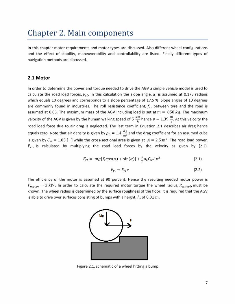
In order to determine the power and torque needed to drive the AGV a simple vehicle model is used to
calculate the road load forces, . In this calculation the slope angle, , is assumed at 0.175 radians
which equals 10 degrees and corresponds to a slope percentage of 17.5 %. Slope angles of 10 degrees
are commonly found in industries. The roll resistance coefficient, , between tyre and the road is
assumed at 0.05. The maximum mass of the AGV including load is set at . The maximum
velocity of the AGV is given by the human walking speed of
hence
. At this velocity the
road load force due to air drag is neglected. The last term in Equation 2.1 describes air drag hence
equals zero. Note that air density is given by
and the drag coefficient for an assumed cube
is given by while the cross-sectional area is given at . The road load power,
is calculated by multiplying the road load forces by the velocity as given by (2.2).
(2.1)
(2.2)
The efficiency of the motor is assumed at 90 percent. Hence the resulting needed motor power is
. In order to calculate the required motor torque the wheel radius, must be
known. The wheel radius is determined by the surface roughness of the floor. It is required that the AGV
is able to drive over surfaces consisting of bumps with a height, , of .
Figure 2.1, schematic of a wheel hitting a bump
8
The force required to pass the bump is calculated by a torque equilibrium between torque due to weight
and torque due to applied force. The designation of the applied force and weight is displayed in Figure
2.1. The relation between required input force, , and wheel radius for a given bump height is given
by the following formula.
(2.3)
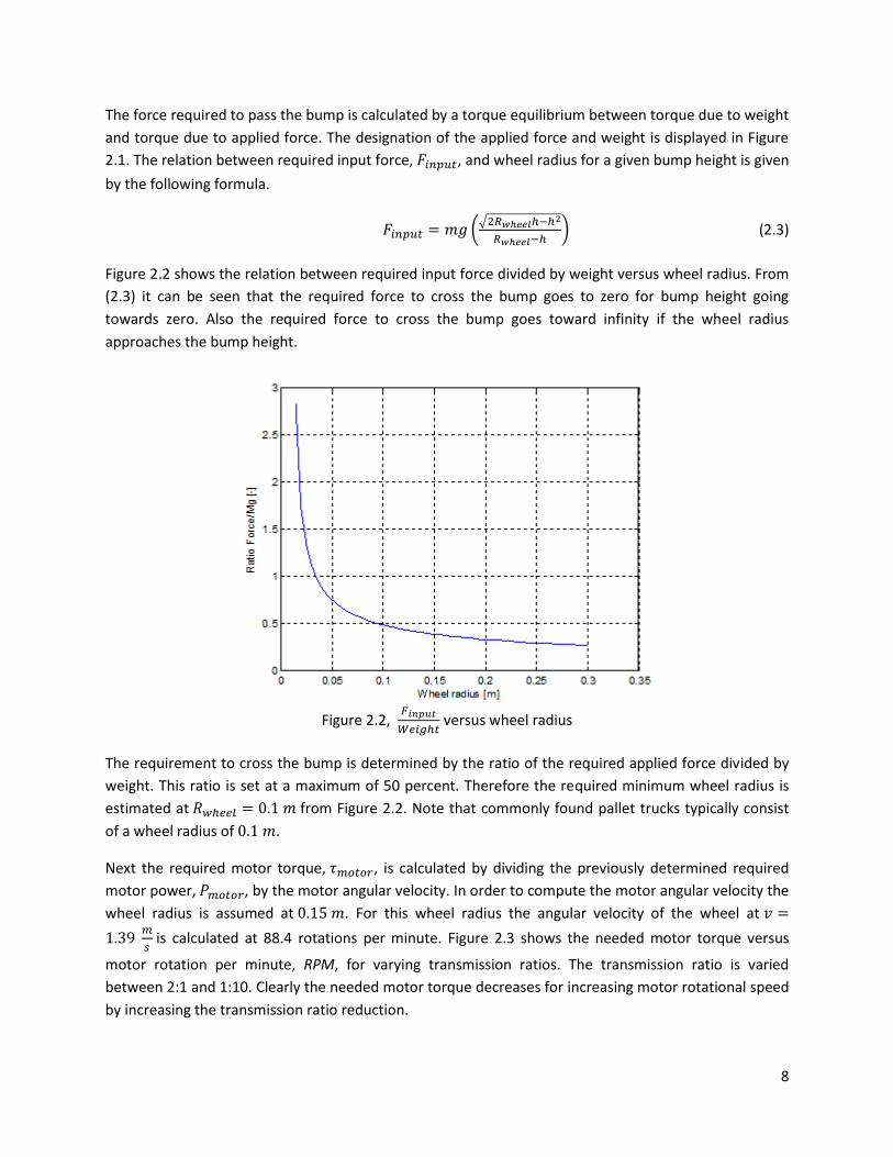
Figure 2.2 shows the relation between required input force divided by weight versus wheel radius. From
(2.3) it can be seen that the required force to cross the bump goes to zero for bump height going
towards zero. Also the required force to cross the bump goes toward infinity if the wheel radius
approaches the bump height.
Figure 2.2,
versus wheel radius
The requirement to cross the bump is determined by the ratio of the required applied force divided by
weight. This ratio is set at a maximum of 50 percent. Therefore the required minimum wheel radius is
estimated at from Figure 2.2. Note that commonly found pallet trucks typically consist
of a wheel radius of .
Next the required motor torque, , is calculated by dividing the previously determined required
motor power, , by the motor angular velocity. In order to compute the motor angular velocity the
wheel radius is assumed at . For this wheel radius the angular velocity of the wheel at
is calculated at 88.4 rotations per minute. Figure 2.3 shows the needed motor torque versus
motor rotation per minute, RPM, for varying transmission ratios. The transmission ratio is varied
between 2:1 and 1:10. Clearly the needed motor torque decreases for increasing motor rotational speed
by increasing the transmission ratio reduction.

9
Figure 2.3, Motor torque versus motor speed for increasing transmission ratio reduction
Without a transmission the motor should be capable of delivering a torque of at an
motor speed of 88.4 RPM in order to overcome the stated road load forces at
. Driving in a
straight line, while using a differential drive configuration, requires the left and right front wheel to be
rotated at the same angular velocity. Therefore it is required to accurately control the rotational speed
of each motor. Note that the wheel radius and traction are considered equal for each wheel.
Furthermore the AGV will be equipped with a battery pack delivering direct current. Therefore a direct
current motor is preferred since no DC-AC inverter is needed. This reduces the number of components
and increases the drive train efficiency since heat losses are lowered. An additional property of electric
motors is to use the motor as a generator. Hence the motors are capable of recovering kinetic energy. A
kinetic energy recovery system is preferred in order to increase the service time of the AGV.
Next the advantages and disadvantages of three commonly used DC motor types are listed.
Torque motor
The main advantage of a torque motor is the possibility to provide high torques at low motor speeds.
Therefore a design without transmission, direct drive, is possible which results in less maintenance costs,
space and mechanical complexity. Also the efficiency is increased since no power is wasted into
transmission friction. Furthermore the stiffness of the drive train is higher because the transmission is
removed and it is able to handle relative high inertias [1]. Drawbacks are higher motor and control costs.

10
Also the control is more complex compared to stepper and servo motors.
Stepper motor
An important advantage of stepper motors compared to servo motors is the larger number of poles
which in result increase the accuracy of the desired position and speed. Note that this only holds if
motor control is designed adequately. Also the torque of a stepper motor at low speeds is higher
compared to a servo motor of equal size. Furthermore the stepper motor is relatively cheap compared
to servo motors but the efficiency is relatively low. Besides these advantages also disadvantages can be
stated for stepper motors. The main disadvantage is the limitation to accelerate a load fast [2]. This is
due because steps may be skipped when the torque of the stepper is too low to move to the next step.
This is resulting in a loss of position and hence positional accuracy is lowered. In general stepper motors
are well suited for low accelerations and applications consisting of high holding torques and low
price.
Servo motor
A servo motor is typically used in a position or speed feedback control system. Servo motors are
available in AC and DC drive [3]. An important advantage of a servo motor is the possibility to be used in
applications which demand high speed and high torque. The efficiency of servo motors is higher
compared to stepper motors. A main drawback of servo motors is the need of a gearbox at low speeds
hence increasing the mechanical complexity. The price of a servo motor is higher compared to a stepper
motor. In general servo motors are well suited for high motor speed and high motor torque applications.
2.2 Effect of wheel configuration on stability and manoeuvrability.
2.2.1 Wheel types
There are many possible wheel configurations when designing possible forms of locomotion. Therefore
before examining possible wheel configurations the wheel is studied. In general there exist four
different wheel types consisting of different degrees of freedom. Therefore the manoeuvrability of the
AGV is influenced by the wheel configuration and the choice of wheel. Figure 2.4 shows the standard
wheel and castor wheel in respectively column A and B. Both the standard wheel and castor wheel have
a primary axis of rotation. The standard wheel has two degrees of freedom namely rotation around the
wheel axle and rotation around the contact point which is normal to ground. The castor wheel consists
of an offset in castor angle with respect to the standard wheel. The castor wheel is able to rotate around
the wheel axle and the offset steering joint. Therefore a castor wheel consists of two degrees of
freedom.

11
Figure 2.4, Four basic wheel types. From left to right: standard wheel, castor wheel, 90 and 45 degrees
Swedish wheel and spherical wheel. [4]
Column C of Figure 2.4 shows a 90 degrees and 45 degrees oriented Swedish wheel. The Swedish wheel
has three degrees of freedom. These degrees of freedom are rotation around the wheel axle, rotation
around the rollers and rotation around the contact point. The Swedish wheel is also called an omni-
wheel since it allows movement in any direction. Column D of Figure 2.4 shows a true omni-directional
wheel which is a spherical wheel. The sphere allows movement in any direction. The spherical wheel
however copes with technical problems related to suspension design. The standard wheel and castor
wheel main advantages are the high tolerance to ground irregularities and the high load capacity. Also
the castor wheel automatically aligns itself to the direction of movement. Due to this aligning movement
the castor wheel exerts an additional reaction force to the chassis. This is considered a drawback since
the stiffness of the chassis should be sufficiently high.
2.2.2 Wheel configuration criteria
The combination of wheel types and wheel configuration governs manoeuvrability, stability and
controllability issues.
Stability
In general stability requires at least 3 wheels in ground contact and the centre of gravity inside the
support angle spanned by the 3 wheels. The stability can be improved by 4 and more wheels. Adding
more than 3 wheels however results in a hyper static situation and therefore a flexible suspension
system is necessary to maintain contact of each wheel to the ground. A simple attempt to approach a
suspension is to include flexibility in the wheel itself. For example a flat terrain consisting of only little
non smoothness can be dealt with by using only deformable soft rubber tyres.
Manoeuvrability
It is desired that the AGV is able to perform tasks with the highest freedom regarding path planning. In

12
the most ideal case an AGV is able to move in any direction of the ground plane. So the AGV is desired to
be omni-directional. Omni-directional movement usually is obtained by using wheels which are actively
powered and are able to move in more than one direction. So the AGV is typically manoeuvrable if it has
a turning radius equal to zero and a swept radius equal to the vehicle length. In this way the AGV is able
to position itself without using parking manoeuvres. So in effect the AGV has three degrees of freedom
namely two translations and one rotation given by longitudinal, translational and yaw displacement.
Controllability
In order for the AGV to behave as a vehicle in terms of path following the wheels are controlled. The
control of the wheels rotation and steering input is needed in order to be able to drive for example in a
straight line. A highly manoeuvrable AGV is in general more difficult to control. This is due to the
relatively high degrees of freedom of the wheels for a manoeuvrable AGV. Therefore some of the
degrees of freedom need to be fixed in order to drive in a straight line for example by using state
feedback. For example a differential drive, as found in a Segway, is highly manoeuvrable but harder to
control. Controlling the differential drive to follow a straight line in general is tricky since even small
deviations in the wheel speeds and wheel radius results in a different path.
2.2.3 Wheel configurations
The manoeuvrability of a robot is composed of the mobility of the structure and an additional freedom
contributed by the steering mechanisms. The degree of manoeuvrability, , is given by the formula
below [5]. Where denotes the degree of mobility and denotes the degree of steerability. The
degree of steerability represents an indirect degree of motion due to the ability of changing the
orientation of the kinematic constraints.
(2.4)
The degree of steerability for a one steered wheel such as a tricycle is equal to one. The degree of
steerability for two steered wheels on a common axis is also equal to one. An example of two steered
wheels on a common axis is for example Ackerman steering in a car. The degree of steerability is equal
to two for a system consisting of two steered wheels with no common axis.
Figure 2.5, Degrees of manoeuvrability for different wheel configurations. [5]

13
Figure 2.5 shows the degrees of manoeuvrability for different wheel configurations. The solid gray
circles denote uncontrollable spherical wheels. The solid gray rectangle denotes uncontrollable standard
wheels. The solid gray rectangle with arrow denotes controllable standard wheels. From the figure
follows that the omni-steer and two-steer configuration consists of manoeuvrability of degree three. So
the configurations are able to manoeuvre the vehicle in all directions from every position and hence
these systems are holonomic. The differential drive and tricycle configuration have manoeuvrability of
degree two. Therefore these systems are non-holonomic and thus manoeuvrability is dependent on the
path taken. When the differential drive is mounted lateral to the geometric midpoint it is able to rotate
on its own axis. Under this condition the differential drive is able to move in all directions after first
rotated into the correct direction. The main drawback of positioning the differential lateral to the own
axis of the vehicle is the risk of the centre of gravity leaving the supporting triangle. Hence guaranteeing
stability becomes tricky. A solution to this issue is to add an additional uncontrollable wheel to the
remaining ‘unwheeled’ edge. Adding an additional wheel results in a total of 4 wheels such that the
system is over determined. Therefore a flexible suspension is needed for example by using flexible
wheels.
An alternative to the tricycle differential drive is found in replacing each wheel by a differential drive
module. Each differential drive module is able to rotate on its own axis resulting in a robot capable of
moving in every direction depending on the orientation of the differential modules as visualized in
Figure 2.6. As stated in Section 2.2.3. high manoeuvrability results in more elaborate control. In effect
the system described in Figure 2.6 needs an additional level of control. This additional level of control is
needed in order to control the robot as a vehicle by sending actuator input to each module. Since VDA
desires an AGV which is cheap and preferably consists of non complex control the differential drive
module robot is not a suitable option. The AGV is preferred to be simple and easy to control. Therefore
modelling is continued by a tricycle differential drive. Also in comparison to the differential drive module
robot no internal dynamics are present in the tricycle because the system is not overdetermined.
Figure 2.6, Possible moving directions of the differential drive module robot. [6]
2.3 Navigation
Navigation can be subdivided into three main categories namely navigation based on odometry,
onboard sensors or external sensor. In odometry the current position is estimated by calculating the
traveled path from the previous location. In general this is done by integrating estimated speeds over
elapsed time. The odometry localization consists of a significant uncertainty due to for example errors in
wheel diameter and limited resolution during integration. Navigation based on external sensors in
general is done by detecting multiple beacons followed by triangulation. Triangulation is made by
measuring angles to the beacons while knowing the distance between the beacons. Therefore one
distance and two angles of a triangle are known resulting in position localization. Navigation based on

14
onboard sensors in general make use of cameras to build up a map of the surroundings while keeping
track of its path using odometry. The position will become uncertain after some movement because the
odometry consist of uncertainties. The position becomes less uncertain again by measuring the local
position by using the onboard sensors. Next navigation techniques based on external and onboard
sensors are discussed.
2.3.1 Navigation based on external sensors
Wired Navigation
Navigation by following a wire in the ground is one of the easiest methods of AGV navigation. This
method uses a wire buried in the floor which transmits a radio frequency. A sensor mounted on the AGV
detects the radio frequency and follows it. The main drawback of this method is the possibility of only
being able to follow the path set by the wire instead of flexible navigation. The sensors are cheap but
preparing the floor of the plant is costly. If only low AGV flexibility is desired wired navigation is suitable.
Guide tape
Navigation by using tape to guide a path is comparable to wired navigation. The main difference is the
replacement of the buried wire by a magnetic or colored tape. The tape is attached at the floor which
reduces the initial investment costs and increases flexibility. The main drawback of wired navigation is
also present for guide tape navigation since the AGV is also only able to follow the path set by the tape.
Furthermore the tape may become damaged or dirty due to wear caused by the crossing vehicles.
Indoor positioning systems
Indoor positioning systems have a higher flexibility by using wireless technologies such as optical, radio
or acoustic methods for position localization by using triangulation. The system is comparable to global
positioning systems but instead of satellites local reference beacons are used. For navigation purposes
also a detailed indoor map is needed next to the position localization. A detailed indoor map is not
always available for a dynamic production plant. Also the system detects the localization but not
necessarily the orientation or direction of the AGV.
2.3.2 Navigation based on onboard sensors
Stereo vision
A stereo vision system often consists of two parallel cameras separated at a known horizontal distance.
Both cameras record the scene at the same moment. Comparison between the left and right image
results in a disparity map which can be translated into a depth image [7]. Hence the stereo vision system
also uses the triangulation principle by viewing the object from two different perspectives. Objects
appear shifted depending on the distance to the camera. The shift in pixels can be converted to depth
information. The advantage of stereo vision is the ability of one shot measurement by comparing only

15
one image pair therefore it can measure moving and still standing objects. Also vision systems are
known for the possibility to extract information on dimension and color and hence applied for
pedestrian recognition in cars. The main drawbacks however are the relatively less detailed 3D
information and high computational costs.
Time of flight cameras
A time of flight camera is able to measure length, width and also depth of an image. The depth of the
image is obtained using the travel time of light. The time of flight camera consist of a light source which
emits light at the scene at a very high frequency up to 100 MHz which is unobservable for humans by
using a near infrared light source. The emitted light reflects objects present in the scene which are
recorded by a camera equipped with a spectrum filter to filter out noise from the environment. The
covered range varies from a few centimeters up to 60 meter. However the resolution decreases for
increasing depth range. Time of flight cameras are able to operate up to a frame rate of 160 images per
second. Therefore time of flight cameras are very well suited to be used in real time applications
because distance can be measured by using only a single shot. Furthermore the system components can
be placed next to each other which results in a compact structure. Distance information is obtained via
an efficient algorithm which only needs relatively low processing power. One of the disadvantages of
time of flight cameras is found in interference. Interference occurs if multiple time of flight cameras are
used simultaneous. Since the measurement may be disturbed by light sources of other cameras. A
solution is found in using different modulation frequencies or by time multiplexing. Another
disadvantage is multiple reflections which result in a measured distance obtained by a detoured light
beam such that the measured distance is greater than the actual distance. Time of flight cameras add
flexibility but are expensive therefore are only suitable if the customer is demanding high AGV flexibility.
As shown in this chapter the maximum speed of the AGV is reached by a motor without transmission by
delivering a motor torque, , of while .
When the differential drive is mounted lateral to the geometric midpoint the AGV is able to rotate on its
own axis. Under this condition the differential drive AGV is able to move in all directions after first being
rotated into the correct direction. Also no internal dynamics are present in the tricycle because the
system is not overdetermined. The AGV is preferred to be manoeuvrable, simple and easy to control.
Therefore the AGV is modelled by a tricycle differential drive.

16
Chapter 3. Simulation packages
The goal of the project is to produce a simulation model describing the dynamical behavior of the AGV.
This simulation model can be used to assess the stability for varying positions of the load. In order to
simulate the AGV model three CAE packages are examined. In Appendix A the numerical accuracy of a
pendulum system in SimMechanics and NX 7.5 Nastran are compared to the analytical solution
simulated using Matlab Simulink. In this comparison Matlab Simulink and SimMechanics utilize a fourth
order Runge-Kutta solver. From this comparison it is concluded to continue by using Nastran because
the absolute error is smaller compared to SimMechanics. Nastran also imposes more geometric
information and allows easier design adjusting compared to SimMechanics.
A simple model of the AGV is obtained by extending the pendulum model of Appendix A by a translating
cart. In this section the numerical accuracy of an inverted pendulum cart system is examined. Therefore
a Simulink model for the inverted pendulum cart system is build using the equations of motion for the
angle of the pendulum and longitudinal position . Also the inverted pendulum cart system is
constructed using NX Nastran and will be compared to the analytical solution of Simulink.
3.1 Analytical model
In order to compare the results obtained using NX Nastran an analytical model is simulated using
Simulink. Simulating the inverted pendulum cart system using Simulink involves deriving differential
equations known as the equation of motions. The equations of motion are derived using the Euler-
Lagrange equations and stated in the next section.
Euler-Lagrange inverted pendulum cart system.
A schematic representation of the inverted pendulum cart system is displayed in Figure 3.1. The mass of
the cart and load are set at and respectively. The length of the massless
pendulum rod is set at . The constant of gravity, , equals
. The rotary joint connecting
the pendulum to the cart consists of a torsion spring, , and torsion damper, . The input force in
longitudinal direction and viscous damping between cart and ground are given by and respectively.
Figure 3.1, Schematic of inverted pendulum cart system.

17
The total kinetic energy, , in the inverted pendulum cart system is given by the following formula.
(3.1)
The total potential energy, P, is given by the following formula.
(3.2)
The Lagrangian is given by the formula given below.
(3.3)
In this case the Euler-Lagrange equation consists of two equations since the inverted pendulum cart
system consist of two free coordinates namely and . The two Euler-Lagrange equations are given
below.
(3.4)
(3.5)
The equations of motion given below are obtained by substituting the derived Lagrangian into (3.4) and
(3.5).
(3.6)
(3.7)
The inverted pendulum cart system is actuated in longitudinal direction located at the cart by a time
dependent input force, , given in Figure 3.2. Note that all initial conditions are set to zero.
Figure 3.2, Input force in longitudinal direction as function of simulation time.
0 5 10 150
100
200
300
400
500
600
700
800
900
1000
Time [s]
Forc
e [
N]
Input force

18
3.2 Comparison case without viscous damping at cart
The differential equations describing the equations of motion of the inverted pendulum cart system
given in (3.6) and (3.7) are used to construct the Simulink model. First the case without damping
between cart and ground,
, and a rigid rotary joint between cart and pendulum is considered.
Hence and are infinity but are set sufficiently high because of simulation purposes. The applied
input force visualized in Figure 3.2 results in the response of the cart displayed in Figure 3.3. Note that
the response obtained by Simulink and Nastran are identical up to machine precision so the response in
position, velocity and acceleration calculated using Nastran are displayed in this figure.
Figure 3.3, Acceleration, velocity and position of the cart due to input force without damping at the cart
using a rigid rotary joint simulated using Nastran.
The resulting acceleration is checked by calculating the acceleration using Newton’s second law,
Equation 3.8.
(3.8)
The force is equal to between and . While the mass of the base and
pendulum substituted is given by . Hence the resulting acceleration is calculated at
.
Figure 3.13 indeed shows an acceleration of
during the corresponding time interval between
and . Also the cart keeps traveling at a constant velocity after the force is applied
due to the absence of damping between cart and ground, this coincides with Newton’s first law.
0 5 10 15-0.5
0
0.5
1
1.5
Simulation time [s]
Accele
ration [
m/s
2]
Acceleration [m/s2]
0 5 10 150
1
2
3
4
5
6
Simulation time [s]
Velo
city [
m/s
]
Velocity [m/s]
0 5 10 150
20
40
60
80
Simulation time [s]
Positio
n [
m]
Position [m]

19
Since the response of the cart follows from Newton’s first law the connection between cart and
pendulum is made flexible. The viscous damping and stiffness in the rotary joint are given by
and
respectively. The response for this case is calculated using Nastran and
visualized in Figure 3.4. The oscillation present in the acceleration and velocity is caused by the swinging
motion of the pendulum. The angular position of the pendulum is displayed in Figure 3.5.
Figure 3.4, Acceleration, velocity and position of the cart due to longitudinal force without damping at
the cart using a flexible rotary joint.
Figure 3.5, Angular position pendulum due to excitation by longitudinal force without damping at the
cart while using a flexible rotary joint.
0 5 10 15-0.5
0
0.5
1
1.5
Simulation time [s]
Accele
ration [
m/s
2]
Acceleration [m/s2]
0 5 10 150
1
2
3
4
5
6
Simulation time [s]
Velo
city [
m/s
]
Velocity [m/s]
0 5 10 150
20
40
60
80
Simulation time [s]
Positio
n [
m]
Position [m]

20
3.3 Comparison case consisting of viscous damping at cart
The cart is also actuated by the force visualized in Figure 3.2 while viscous damping,
is
present between cart and ground. The response of the cart is displayed in Figure 3.6. In this figure the
response calculated by Simulink and Nastran are displayed by the smooth and dashed lines respectively.
This case resembles the effect of initially accelerating the cart and slowing down due to viscous damping
until the cart velocity is zero. Clearly the acceleration becomes negative after the magnitude of the input
force decreases. As a result the velocity of the inverted pendulum cart system starts to decrease.
Ultimately leading the system to reach an equilibrium in longitudinal position between and . The
calculated angular position of the pendulum for both simulation methods is displayed in Figure 3.7. In
comparison to the case without viscous damping,
, the pendulum also swings into positive
angular position instead of only into negative angular position. This motion is due to the inertia of the
pendulum mass while the cart decelerates by the viscous damping between cart and ground.
Figure 3.6, Acceleration, velocity and position of the cart due to longitudinal force under presence of
viscous damping between cart and ground using Simulink and Nastran.
0 5 10 15-0.6
-0.4
-0.2
0
0.2
0.4
0.6
0.8
Simulation time [s]
Accele
ration [
m/s
2]
Simulink acceleration [m/s2]
Nastran acceleration [m/s2]
0 5 10 150
0.5
1
1.5
2
Simulation time [s]
Velo
city [
m/s
]
Simulink velocity [m/s]
Nastran velocity [m/s]
0 5 10 15
0
2
4
6
8
10
Simulation time [s]
Positio
n [
m]
Simulink position [m]
Nastran position [m]

21
Figure 3.7, Angular position pendulum due to input force under presence of viscous damping between
cart and ground using Simulink and Nastran.
In order to compare both simulation methods the relative change between both methods is calculated.
The relative change in longitudinal position, , is given by the formula stated below.
(3.9)
Calculating the relative change at each time step leads to Figure 3.8. From this figure follows that the
maximum relative change is equal to which corresponds to a maximum procentual error of
. The relative change goes towards the error tolerance for increasing simulation time since
the system is at equilibrium.
Also the relative change in angular position, , is given by the next formula.
(3.10)
Calculating the relative change at each time step leads to Figure 3.9. From this figure follows that the
maximum relative change is equal to which corresponds to a maximum procentual error of
. The relative change goes towards the error tolerance for increasing simulation time since the
system is at equilibrium. The error tolerance specified in Simulink and Nastran corresponds to a
procentual error of of . This error tolerance is visible by the block patern in the osciliation

22
between 10 and 15 seconds. Hence the use of Nastran is verified and it is concluded to use Nastran to
conduct simulations described in the remainder of the report.
Figure 3.8, Relative change in Figure 3.9, Relative change in
longitudinal position between angular position between
Simulink and Nastran model. Simulink and Nastran model.
As shown in this chapter NX Nastran is capable and verified to conduct motion simulations. This verification is done by comparing the analytical solution of an inverted pendulum cart system to the results obtained by NX Nastran. As shown the verification is split up in three parts ranging from a case without viscous damping to a case consisting of viscous damping at the pendulum and between cart and ground. A quantitative comparison is made for the case of the inverted pendulum cart system consisting of stiffness and viscous damping at the pendulum and viscous damping between cart and ground. As shown the relative change in angular position between the Simulink and Nastran model goes towards the error tolerance specified for the system when reaching equilibrium. Hence the use of Nastran is verified and Nastran is used to conduct simulations described in the remainder of the report.
23
Chapter 4. Dynamic behavior
In this chapter the dynamic behavior of the system is examined for varying system parameters. First
research is done into the inverted pendulum cart system. Next research is done into the cart-mass
system.
4.1 Research on inverted pendulum cart system
The use of NX Nastran to conduct dynamical simulations is verified in the previous section. Therefore NX
Nastran is used to investigate the dynamical behavior of mechanical systems. In this section the
dynamical behavior of the inverted pendulum cart system is investigated for varying system parameters.
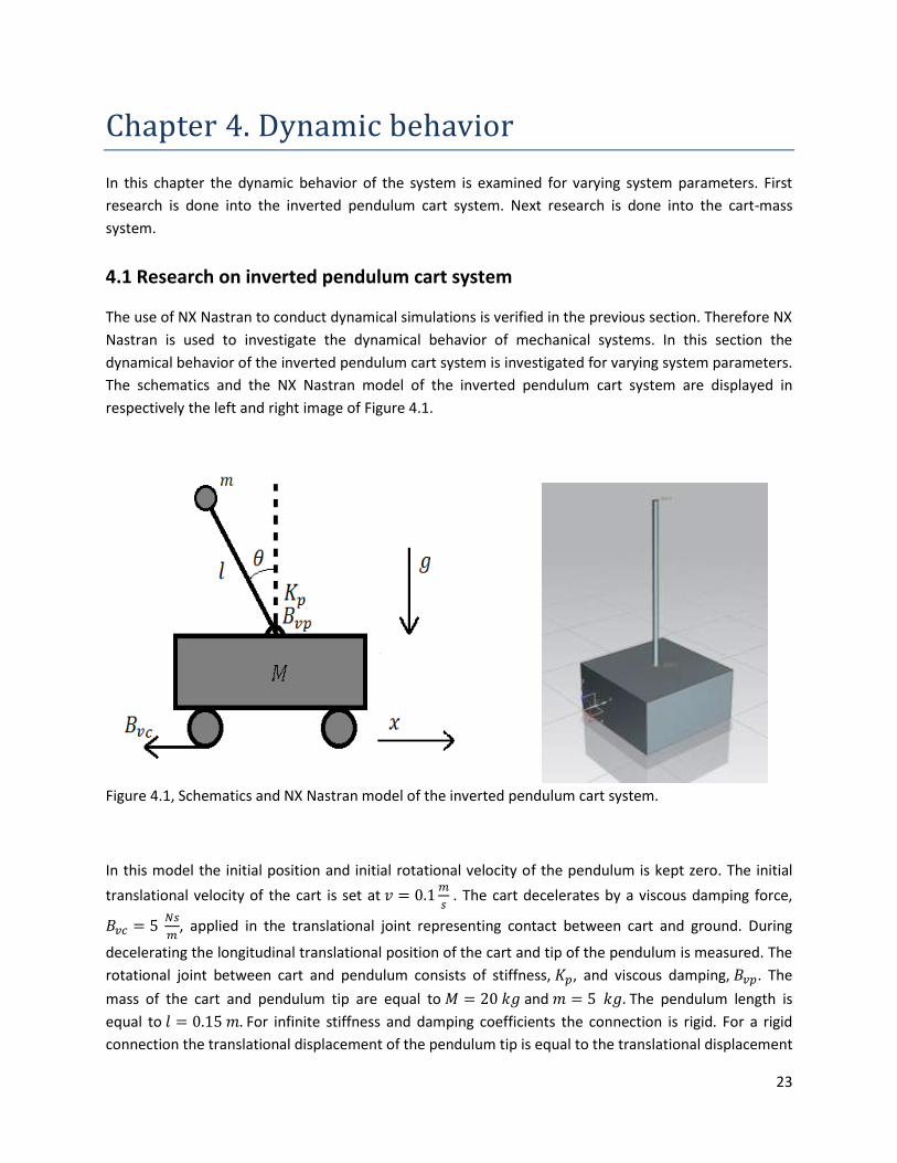
The schematics and the NX Nastran model of the inverted pendulum cart system are displayed in
respectively the left and right image of Figure 4.1.
Figure 4.1, Schematics and NX Nastran model of the inverted pendulum cart system.
In this model the initial position and initial rotational velocity of the pendulum is kept zero. The initial
translational velocity of the cart is set at
. The cart decelerates by a viscous damping force,
, applied in the translational joint representing contact between cart and ground. During
decelerating the longitudinal translational position of the cart and tip of the pendulum is measured. The
rotational joint between cart and pendulum consists of stiffness, , and viscous damping, . The
mass of the cart and pendulum tip are equal to and The pendulum length is
equal to For infinite stiffness and damping coefficients the connection is rigid. For a rigid
connection the translational displacement of the pendulum tip is equal to the translational displacement
24
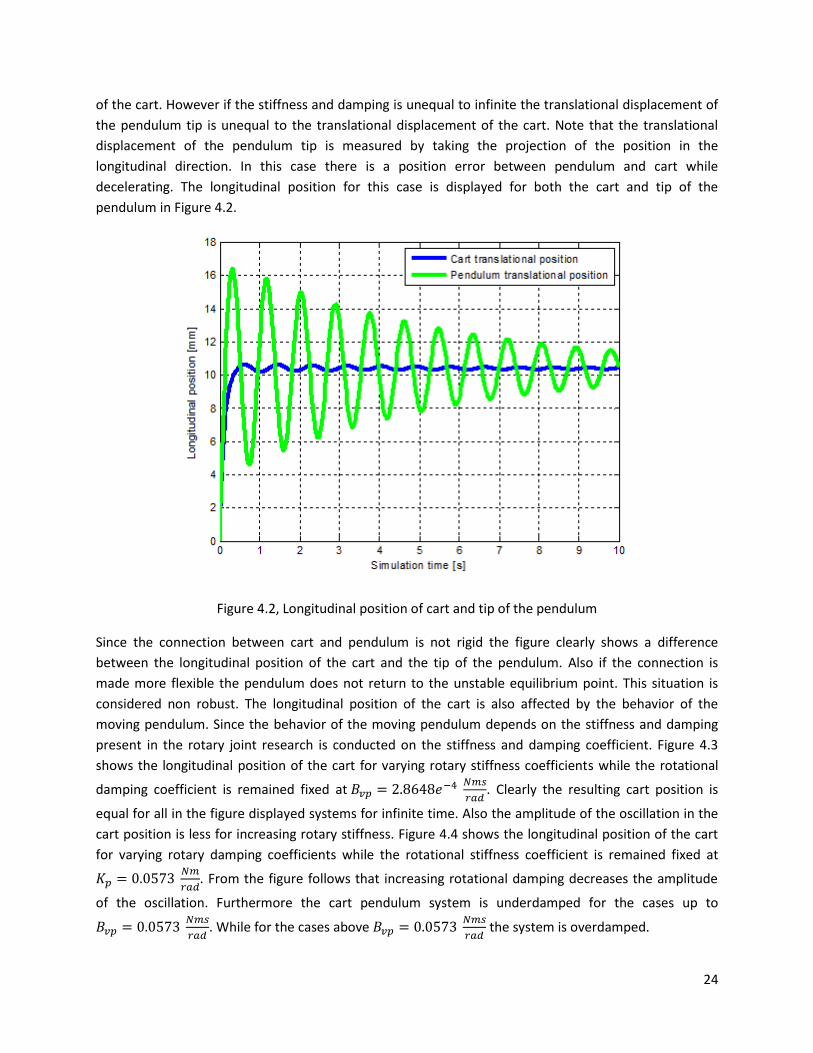
of the cart. However if the stiffness and damping is unequal to infinite the translational displacement of
the pendulum tip is unequal to the translational displacement of the cart. Note that the translational
displacement of the pendulum tip is measured by taking the projection of the position in the
longitudinal direction. In this case there is a position error between pendulum and cart while
decelerating. The longitudinal position for this case is displayed for both the cart and tip of the
pendulum in Figure 4.2.
Figure 4.2, Longitudinal position of cart and tip of the pendulum
Since the connection between cart and pendulum is not rigid the figure clearly shows a difference
between the longitudinal position of the cart and the tip of the pendulum. Also if the connection is
made more flexible the pendulum does not return to the unstable equilibrium point. This situation is
considered non robust. The longitudinal position of the cart is also affected by the behavior of the
moving pendulum. Since the behavior of the moving pendulum depends on the stiffness and damping
present in the rotary joint research is conducted on the stiffness and damping coefficient. Figure 4.3
shows the longitudinal position of the cart for varying rotary stiffness coefficients while the rotational
damping coefficient is remained fixed at
. Clearly the resulting cart position is
equal for all in the figure displayed systems for infinite time. Also the amplitude of the oscillation in the
cart position is less for increasing rotary stiffness. Figure 4.4 shows the longitudinal position of the cart
for varying rotary damping coefficients while the rotational stiffness coefficient is remained fixed at
. From the figure follows that increasing rotational damping decreases the amplitude
of the oscillation. Furthermore the cart pendulum system is underdamped for the cases up to
. While for the cases above
the system is overdamped.

25
Figure 4.3, Longitudinal position of cart for varying rotary stiffness and fixed
.
Figure 4.4, Longitudinal position of cart for varying rotary damping and fixed

26
In order to assess the tracking behavior between pendulum tip and cart the relative change is calculated
and is given by the following formula.
(4.1)
Where and denotes respectively the longitudinal position of the cart and the translational position
of the pendulum tip. The relative change as function of the simulation time is calculated for
and
and displayed by blue line in Figure 4.5. Clearly the relative
change between pendulum tip and cart goes towards zero for increasing simulation time. This is because
the cart decelerates from
to zero whereas the amplitude of the pendulum oscillation
decreases due to the damping present in the rotary joint and the slider joint present between cart and
ground. Note that the displayed decrease in relative change in longitudinal position is not only caused by
viscous damping present in the rotary joint between cart and pendulum. This is due to the additional
dissipation of energy caused by the viscous damper in the slider joint. For increasing rotary damping the
relative change is lower at each simulation time as displayed by the red line in Figure 4.5.
Figure 4.5, Relative change in longitudinal position between pendulum tip and cart.
In order to compare the effect of rotary stiffness and rotary damping on the relative change in
longitudinal position the maximum of the absolute value of the relative change is calculated. This is
done for every combination of stiffness and damping and displayed in Figure 4.6 and Figure 4.7

27
respectively. From the Figures it can be seen that for high joint stiffness and high joint damping
coefficients the relative change is low hence the cart pendulum system is rigid. Moreover the relative
change is low for damping coefficients above
. This indeed corresponds to
overdamped cart pendulum systems for fixed rotary stiffness at
.
Figure 4.6, Maximum of relative change for varying and fixed
.
Figure 4.7, Maximum of relative change for varying and fixed
.

28
4.2 Research on cart-mass system
The previous section described the dynamical behavior of the cart pendulum system for varying system
parameters. In this section the dynamical behavior of a cart connected to a mass using a slider joint is
examined. Again the dynamical behavior of the system is investigated for varying system parameters
which in this case are viscous damping, , and stiffness, , between cart and mass. The schematics
and NX Nastran model of the cart-mass system are displayed in the left and right image of Figure 4.8
respectively.
Figure 4.8, Schematics and NX Nastran model of cart-mass system
In this model the initial velocity of the cart is equal to the maximum traveling velocity of the AGV which
is
. The cart decelerates by a viscous damping force,
applied in the translational
joint between cart and ground representing braking. The value of is set such that the cart-mass
system consists of a braking distance around a maximum of 1 meter. A maximum braking distance of 1
meter at full speed is used because of AGV safety considerations. The mass of the cart and mass are
given by and respecitvely. After a delay the velocity of the mass decreases as
well. This delay is due to inertia of the mass. Because of the inertia a tracking error in longitudinal
position occurs between cart and mass. This tracking error depends on the magnitude of the stiffness
and viscous damping between cart and mass. In order to visualize the effect of viscous damping, ,
between cart and mass the stiffness is set constant to
. Figure 4.9 shows the longitudinal
position of both the cart and the mass as function of simulation time. In this figure the viscous damping
between cart and mass, , is varied between
and
The figure shows that the
longitudinal position of the mass is indeed higher compared to the cart position. A quantitative analysis
is made by calculating the relative change in longitudinal position between cart and mass (4.1) and is
displayed in Figure 4.10. The figure shows that the relative change increases for decreasing viscous
damping, hence the system becomes more flexible. Also the relative change goes toward zero for long
simulation times, since the system is at rest.

29
Figure 4.9, Longitudinal position of mass and cart for fixed stiffness
.
Figure 4.10, Relative change in longitudinal position for fixed stiffness
.
Next the viscous damping is fixed at
while the stiffness between cart and mass, , is
varied between
and
. All remaining system parameters are kept equal. The resulting
longitudinal position of both the cart and the mass as function of simulation time is displayed in Figure

30
4.11. The figure also shows that the position of the mass is further compared to the cart. The final
position of every system is around and hence within the specified braking distance of one meter.
Again a quantitative analysis is performed by calculating the relative error in longitudinal position
between cart and mass, see (4.1), and this is displayed in Figure 4.12. This figure clearly shows a
decrease in error for increasing stiffness. This is because increasing the stiffness results in a more rigid
system. Hence the tracking error between cart and mass become smaller for increasing stiffness and
increasing viscous damping. Consider the load given by the pendulum and mass. Hence this chapter
concludes that the tracking error between cart and load decreases for increasing stiffness and damping.
This is because the connection between cart and load becomes more rigid. If the tracking error between
cart and load becomes sufficiently high the load will disconnect from the cart. Therefore a rigid
connection between cart and load is desired in the final AGV design.
Figure 4.11, Longitudinal position of Figure 4.12, Relative change in
mass and cart for fixed viscous longitudinal position for fixed
damping
. viscous damping
.
As shown in this chapter the dynamic behavior of the system is examined for varying system parameters.
This is done for both an inverted pendulum cart system and a cart-mass system. For the inverted
pendulum cart system high joint stiffness and high joint damping coefficients results in a low relative
change in longitudinal position hence the cart pendulum system is rigid. Moreover the relative change is
low for damping coefficients above
. This indeed corresponds to overdamped cart
pendulum systems for fixed rotary stiffness at
.
Also for the cart mass system the tracking error between cart and mass becomes smaller for increasing
stiffness and increasing viscous damping between the cart and mass. Which is due because the
connection between cart and load becomes more rigid. The load will disconnect from the cart if the
tracking error between mass and cart is sufficiently high. Hence the AGV is desired to have a rigid
connection between cart and load.

31
Chapter 5. The AGV model
The previous section described dynamical behavior of the inverted pendulum cart system and the cart
mass system. In this section the previous Nastran models are extended into a differential drive tricycle
model describing the AGV. Therefore first the effect of the differential position on the cornering radius is
examined followed by the dimensions of the AGV. In the remainder of this chapter simulations using the
AGV model are discussed.
5.1 Cornering radius
In order to be able to determine the cornering radius of the tricycle mobile robot assumptions on wheel
kinematic constraints are made. First of all the wheel is only able to move in the horizontal plane. Also
the geometry of the wheel is rigid and therefore undeformable. The contact point of the wheel with the
ground is assumed to be a point contact. The wheel motion is pure rolling hence no slipping, sliding or
skidding occurs. Furthermore the connection between wheel and chassis is rigid.
The degree of steerability for the differential drive tricycle is zero because the castor wheel is unsteered.
While the degree of mobility is equal to two and is given by the longitudinal and rotational direction.
Hence by using Equation 2.4 the degree of maneuverability of the AGV is two. The instantaneous centre
of rotation of the mobile robot is therefore constrained on a line, which is the axis of the differential
wheels. The distance between differential centre and instantaneous centre of rotation is called the
cornering radius of the differential centre, , given by the formula given below.
(5.1)
The mobile robot will rotate around the differential centre if the translational velocity of the left wheel
is opposite equal to the translational velocity of the right wheel respectively given by and . The
track width, , of the AGV is equal to . Also the cornering radius of the differential centre is
infinity if the translational velocity of the left wheel is equal to the right wheel. Hence the mobile robot
drives in a straight line if both wheels are driven at equal translational velocity. The cornering radius of
the AGV is calculated with respect to the geometric midpoint instead of the differential centre. However,
the differential centre is displaced at a longitudinal offset with respect to the geometric midpoint. The
cornering radius of the geometric midpoint is denoted as.
(5.2)
The resulting minimal cornering radius of the mobile robot is therefore equal to the size of the offset
between centre of gravity and differential centre. Figure 5.1 shows the cornering radii for the
differential centre and centre of gravity for two offsets. For visualization purposes the translation

32
velocity of the left wheel is fixed at
while the velocity of the right wheel is varied. Clearly the
cornering radius is minimal if the translational velocity of the right wheel equals
. Also the
cornering radius is maximal if the translational velocity of the right wheel equals
.
Figure 5.1, Cornering radii for varying while
.
5.2 The AGV model in NX Nastran
The AGV is modeled as a tricycle consisting of a rear differential drive and a front castor wheel. The
offset between differential drive and geometric midpoint equals and is given by . The
AGV consists of a cart and a load. In the cart a modular base is present to which the load is attached. The
connection between load and modular base relies solely on friction because accelerations are relatively
low. Therefore the modular base is covered by a rubber like material consisting of a sufficient high
friction force between both bodies due to the weight of the load. The gravity acts in negative z-direction
while the static and dynamic coefficients of friction of the load are given by and
respectively. The sum of the mass of the cart and modular base is given by
while the mass of the load, , is given by . The dimensions of the AGV are displayed
by the side view and top view in Figure 5.2. Note that in this figure the dimension of the load is equal to
the maximum size of a standard euro pallet and is visualized by the gray block. The centre of gravity of
the cart is fixed and visualized by the checkered circle. The centre of gravity of the load depends on the
position of the load and therefore is free and examined in the later.

33
Figure 5.2, Side view and top view of the AGV dimensions.
Wheel model
The wheels of the AGV are modeled in Nastran by a cylinder which is in contact with the ground using a
Nastran connection named 3D contact. When a pair of solid bodies comes into contact a contact force is
generated by this connection type. Using this joint it is also possible to specify friction between wheel
and ground. The friction model of the tyre is chosen simple because of avoiding large computation times.
The static and kinematic coefficients of friction for a normal tyre on dry concrete are given by
and respectively [15]. The computation time of the simulation
however increases to hours for high friction coefficients. Therefore the worst case scenario of an AGV
driving on ice is considered resulting in and . The wheel model is
displayed in Figure 5.3. This wheel represented by the cylinder is connected to a wheel shaft by a rotary
joint. The input torque is applied at this rotary joint as well. Both left wheel and right wheel are actuated
at an input torque of . The wheel shaft is connected to a small block by a slider joint.
This slider joint consists of stiffness and damping representing the wheel characteristic given by
and
respectively. The small block is used to be able to attach a

34
universal joint between the slider joint and the cart. This is necessary since it is not possible to connect
two joints directly. This small block is connected to an identical small block present in another wheel by
using a parallel constraint. Consequently also the wheel shaft and wheel remains in position. This allows
the cart to pitch, roll and yaw while each wheel is also able to move in z-direction independently. The
cart is able to translate in x and y direction for low friction between wheel and ground. Also the wheels
are able to rotate on the revolute axis resulting in a total of 11 degrees of freedom in the AGV system.
Figure 5.3, Wheel model in NX Nastran of the AGV.
5.3 Simulations AGV model
This section describes NX Nastran motion simulations conducted using the AGV model described in the
previous section. Therefore the input torque of the left and right wheel are both open loop controlled at
a fixed value of .
Linear velocity
The linear velocity of the AGV is calculated by dividing the sum of the magnitude of the left and right
differential wheel velocity by two as given by the formula below.
(5.3)
The calculated linear velocity is displayed by the black line in Figure 5.4. The magnitude of the velocity
for the left wheel and right wheel are given by the green and red line respectively. In NX Nastran it is
also possible to measure the linear velocity directly at a marked point of the system. In this case the
linear velocity of the geometric midpoint is displayed by the blue line. The calculated linear velocity is
indeed equal to the measured linear velocity. Therefore it is possible to measure the linear velocity
directly at a specified point of the system. Note that both left and right wheel are actuated by the same
input torque and hence differences in velocity occur due to differences in traction between both wheels.

35
Figure 5.4, Comparison calculated linear velocity to measured linear velocity at geometric midpoint.
Yaw velocity
The formula of yaw velocity of the AGV is calculated by dividing the difference of the magnitude of the
left and right differential wheel by the track width and is given below. The track width, , is taken to
.
(5.4)
The calculated yaw velocity is displayed by the green line in Figure 5.5. In NX Nastran it is also possible to
measure the yaw velocity directly at a marked point of the system. In this case the yaw velocity of the
geometric midpoint is displayed by the blue line. The calculated yaw velocity is indeed equal to the
measured yaw velocity. Therefore it is possible to measure the yaw velocity directly at a specified point
of the system.
Figure 5.5, Comparison calculated yaw velocity to measured linear velocity at geometric midpoint.

36
Pitch and roll dynamic
Because of the previously described wheel model the AGV consists of 11 degrees of freedom. The
vehicle model is capable of showing pitch and roll dynamics resulting from load offsets and accelerations
due to input torque. Figure 5.7 and Figure 5.8 show respectively the pitch angle and the roll angle as
function of simulation time. The used AGV parameters are listed above while the static and kinematic
coefficients of friction for a normal tyre on dry concrete are used given by and
respectively. In order to enhance the pitch angle the centre of gravity of the load is
displaced by in negative x-direction with respect to the geometric centre of the load. The rear
axle carries more load relative to the vertical axle stiffness compared to the front axle. In combination
with the input torque applied at the rear axle the AGV pitches. The traveled path of the centre of gravity
of the AGV is visualized in a x,y-plot displayed in Figure 5.6. The figure shows that the of the AGV
does not follow a straight line. The roll angle increases because of the increase in yaw velocity due to
traction differences between both differential wheels which is possibly due to a difference in initial
condition specified by Nastran in solving the 3D Contact. The next section discusses the effect of traction
on yaw velocity and displacement.
Figure 5.6, x,y-position CoG AGV
Figure 5.7, Pitch dynamics AGV Figure 5.8, Roll dynamics AGV

37
Linear velocity and yaw rate for varying centre of gravity of the load.
In this section the centre of gravity, CoG, of the load is translated in longitudinal position. First a
reference case is simulated. The reference case consists of a CoG located in the centre of the load. Next
the centre of gravity is translated in longitudinal direction by -0.35 m and +0.2 m denoted by a black and
red line respectively in Figures 5.9, 5.10 and 5.11. The effect on linear velocity and yaw velocity are
displayed in the Figure 5.9 and 5.10 respectively. The resulting angular displacement is visualized in
Figure 5.11. The figures show that for an increasing offset in longitudinal direction, with respect to the
centre, an increasing deviation in linear velocity and yaw rate are resulting. Hence the angular
displacement is increases for increasing offset. Due to this error in angular displacement motor feedback
control will be needed in the AGV. This is because open loop control by setting equal input torque at
each wheel will not guarantee straight line driving because of traction differences between left and right
wheel. The effect of traction differences is exaggerated because of the low friction between tyre and
road.
For comparison the static and kinematic coefficients of friction for a normal tyre on dry concrete results
in the green line in Figure 5.9, 5.10 and 5.11. In effect the maximum yaw displacement under normal
conditions, high friction, is a factor 600 less compared to low friction coefficients, which is the worst
case situation of driving on ice. In this case however the AGV is also not capable of perfect straight line
driving without feedback control but the yaw displacement is decreased significantly resulting in less
control effort.
Figure 5.9, Linear velocity for reference case and translated CoG in longitudinal direction.

38
Figure 5.10, Yaw velocity for reference case and translated CoG in longitudinal direction.
Figure 5.11, Yaw displacement for reference case and translated CoG in longitudinal direction.
Stability positions of load
In this section the stability of the positions of the load is simulated for the cart described in section 5.2
and visualized in Figure 5.12. Note that each simulation is conducted using the same initial conditions.
The input torque of both differential drive wheels is set at . The centre of mass and inertia is
varied in the region of the euro pallet, denoted by the gray block in Figure 5.2 and the blue lines in

39
Figure 5.12. The load is considered stable if the normal force at each wheel is larger than zero Newton.
Hence the centre of gravity of the total system lies within the stability triangle denoted by the black lines
in Figure 5.12. Note that because of symmetry the CoG of the load is only varied at half of the lateral
direction of the pallet. The stable and unstable centers of gravity of the load are visualized by a green
and red dot respectively. In general the load is stable if the CoG lies within the supporting
triangle while the height of the CoG of the pallet lies less than 1 meter above the cart. The allowed
height of the CoG goes up if the CoG lies closer to the geometric midpoint of the longitudinal and lateral
direction of the pallet.
Figure 5.12, Stable and unstable positions CoG of the load
As shown in this chapter the minimal cornering radius of the mobile robot is equal to the size of the
offset between centre of gravity and differential centre. The AGV is modeled as a tricycle consisting of a
rear differential drive and a front castor wheel located at an offset of resulting in a cornering
radius of . The total AGV model consists of 11 degrees of freedom. The AGV is able to pitch, roll
and yaw while each wheel is also able to move in z-direction independently. Also the AGV is able to
translate in x and y direction for low friction between wheel and ground.
Because of computational reasons a simple tyre model is used together with a relatively low coefficient
of static and dynamic friction. Straight line driving is not achieved by only using open loop control
therefore feedback control is needed on the actual AGV.
The stability of the load is dependent on the location of the of the load as shown in this chapter. In
general the load is stable if the CoG of the load lies within the supporting triangle while the
height of the CoG of the load lies less than 1 meter above the cart.

40
Chapter 6. Conclusions and recommendations
6.1 Conclusions
The main goal of this report is to develop a simulation model for the vehicle dynamics of the AGV.
Therefore two CAE packages are compared on numerical accuracy and ease of use. Both packages are
compared to analytical solutions simulated using Matlab Simulink. From this chapter is concluded to
simulate the vehicle model using NX 7.5 Nastran. Because the maximum of the absolute error is a factor
7.2 smaller compared to SimMechanics for a pendulum system consisting of input torque and friction.
Also NX Nastran is verified because the magnitude of the relative change becomes equal to the error
tolerance for the inverted pendulum cart system consisting of initial velocity and viscous damping
between cart and ground. NX Nastran also imposes more geometric information and allows easier
design adjusting compared to SimMechanics. Furthermore the part file created for the motion
simulation in the NX 7.5 environment can easily be exported to the FEM module in order to conduct
simulations on strength and stiffness. Hence the need to transfer data to an external application is
eliminated because the motion model is synchronized with the current design sharing the same
geometric data. Furthermore it is possible to integrate controls into the motion model through co-
simulation with Matlab Simulink.
Research is done on the verified inverted-pendulum cart system by means of varying the stiffness and
damping parameters in the rotary joint connecting the pendulum to the cart. The resulting longitudinal
position of the pendulum tip was compared to the longitudinal position of the cart. The difference in
longitudinal position between pendulum tip and cart decreases for increasing stiffness and damping in
the rotary joint. Hence the connection becomes more rigid. The same observation holds for the cart-
mass system because the difference in longitudinal position between mass centre and cart decreases for
increasing stiffness and damping parameters.
The NX Nastran simulation model of the AGV consists of a differential drive and a front castor wheel in a
tricycle configuration. The tricycle is considered stable if the centre of gravity of the total system lies
within the supporting triangle of the wheels. The system is actuated by input torque at both wheels of
the differential drive. The tricycle design consists of a maneuverability of degree two and hence is non-
holonomic since no movement is possible in lateral direction without slipping of the wheels. The
cornering radius is equal to the longitudinal offset between differential centre and geometric midpoint.
Therefore it is recommended to relocate the differential drive at the geometric midpoint such that the
AGV can turn around its own axis if desired for future applications such as lifting and towing carts. In this
case also a second castor wheel needs to be added to the ‘unwheeled’ edge in order to assure stability.
As a result a flexible suspension system is needed to guarantee contact to the ground for each wheel.
The suspension system might be sufficient by using only flexible wheels at a flat floor. The maximum
velocity and total mass of the AGV are given by
and respectively. The required motor
power is while a motor torque of is demanded without transmission and a wheel radius
equal to

41
The simulated AGV model shows pitch, roll and yaw dynamics. The AGV is not able to follow a straight
line by only applying equal open loop input torque at each wheel of the differential drive. Therefore
feedback control on the input torque is needed to enable straight line driving and trajectory following.
The recommended feedback loop needs to compare the intended direct to the actual direction. The
actual direction can be estimated by inputting the measured lateral acceleration, measuring vehicle yaw
and individual road wheel speeds in a vehicle model.
Also the AGV model is used to assess stability of the load by varying the CoG of the load. In general the
load is stable if the CoG lies within the supporting triangle while the height of the CoG of the
pallet lies less than 1 meter above the cart. The allowed height of the CoG goes up if the CoG lies closer
to the geometric midpoint of the longitudinal and lateral direction of the pallet. The load cannot be
transported on the AGV if the centre of gravity lies outside the specified volume of stability.
6.2 Recommendations
The AGV is equipped with a changeable modular base. In this report the modular base of the AGV is
simplified as being a conveyor belt on which the load is fixed on the AGV. In the case of an unstable load
position the modular base consisting of a conveyor belt can be replaced by a modular base consisting of
a connecting mechanism. This connecting mechanism can be used to connect into a wheeled rack.
Hence the AGV tows the load while it is fixed on the rack instead of carrying the load directly on the
conveyor belt. In this configuration also robotic systems such as robotic arms and palletizers are
transportable and employable simultaneously.
Further research can be split up in two main topics namely mechanical design and control design. In the
mechanical design the differential drive tricycle can be used to compare the case consisting of a
differential drive castor wheel instead of a regular castor wheel. Also the chassis and the required
battery packages can be designed and selected.
The control design will focus on developing a two level control architecture. The low level control
describes a feedback controller controlling the movement of the AGV according to the tracking error
between desired and actual path. The high level control describes the hierarchy between the separate
AGVs. The high level control should schedule the AGVs such that tasks are performed in the shortest
time and preferably the most energy efficient way.
42
Appendix A. Numerical accuracy comparison between Simulink, SimMechanics and Nastran.
In order to compare the numerical accuracy between Simulink and SimMechanics a simple dynamical
system is modeled and simulated. The reason of using a simple dynamical system is found in the ability
of deriving the equations of motion for such a system using Euler-Lagrange equations. For a given initial
condition these equations of motion can be simulated using Simulink and will be compared to the
solution obtained by using SimMechanics and NX Nastran in the later.
A.1 Euler-Lagrange Equations for pendulum
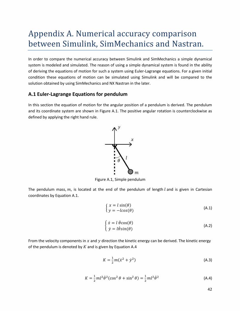
In this section the equation of motion for the angular position of a pendulum is derived. The pendulum
and its coordinate system are shown in Figure A.1. The positive angular rotation is counterclockwise as
defined by applying the right hand rule.
Figure A.1, Simple pendulum
The pendulum mass, , is located at the end of the pendulum of length and is given in Cartesian
coordinates by Equation A.1.
(A.1)
(A.2)
From the velocity components in and direction the kinetic energy can be derived. The kinetic energy
of the pendulum is denoted by and is given by Equation A.4
(A.3)
(A.4)

43
The potential energy is minimum if the pendulum is in the single stable equilibrium located at .
Therefore at this position the potential energy is defined zero. The potential energy is at maximum if the
pendulum is located at the unstable equilibrium located at . Hence the potential energy of
the pendulum is given by Equation A.5.
(A.5)
The Lagrangian is given by subtracting the kinetic energy from the potential energy as given in Equation
A.7.
(A.6)
(A.7)
The Euler-Lagrange equation is given by Equation A.8. Note that in this case the Euler-Lagrange equation
only consists of one equation because the pendulum consists of only one free coordinate. Therefore
only one equation of motion is obtained which is the Euler-Lagrange equation for . Moreover energy is
conserved due to the absence of dissipative forces.
(A.8)
(A.9)
(A.10)
The latter differential equation, Equation A.10, is used to construct the Simulink model displayed in
Figure A.2.
Figure A.2, Simulink model of equation of motion for .

44
Analog to the Simulink model for the pendulum the model constructed using SimMechanics is given by
Figure A.3. Constructing a model in SimMechanics is achieved by specifying physical elements instead of
algorithm elements. Therefore the mechanical system is constructed from blocks representing bodies,
joints, constraints, actuators and sensors. The equations of motion are calculated by SimMechanics from
the physical elements.
Figure A.3, SimMechanics model of the Pendulum
The difference in angular position for both models is displayed in Figure A.4. Clearly simulation using
Simulink is equal to simulation using SimMechanics. Differences however arise for large mass, lengths
and simulation time. These numerical errors are due to magnification of numerical errors in for example
the initial conditions caused by the machine precision.

45
Figure A.4, Difference in angular position between Simulink and SimMechanics model for pendulum
A.2 Comparison case pendulum with friction.
In the case of friction the Lagrangian remains unchanged and therefore is equal to Equation A.7. The
equation of motion however is changed due to a spring and viscous damping term and is given by
Equation A.12.
(A.11)
(A.12)
The latter differential equation is again constructed into a Simulink model and displayed in Figure A.5.
Also the SimMechanics model is updated to the case consisting of friction. In this simulation the
pendulum mass, , and length, , are respectively and . The initial position and velocity of the
pendulum are zero radians and
radians per second respectively. The constant of gravity, , is set at
. The spring and viscous damper are modeled by adding a Joint Spring & Damper block. In this
block the torsion spring is modeled by specifying a spring constant equal to
. Furthermore
the viscous damping is modeled by specifying a damper constant equal to
. The
SimMechanics model is displayed in Figure A.6.
0 10 20 30 40 50 60 70 80 90 100-4
-3
-2
-1
0
1
2
3
4x 10
-10
Simulation time [s]
Diffe
rence in a
ngula
r positio
n [
rad]

46
Figure A.5, Simulink model of pendulum consisting of torsion spring and viscous damping.
Figure A.6, SimMechanics model of pendulum consisting of torsion spring and viscous damping.
The pendulum system is simulated for 5 seconds for three simulation packages. The simulation packages
used are Matlab Simulink, SimMechanics and NX Nastran. The response in angular position for the
stated simulation parameters is displayed in Figure A.7 for all considered simulation packages.

47
Figure A.7, Angular position of the pendulum consisting of friction for three simulation packages.
Figure A.7 shows that each simulation package outputs a comparable oscillation. In order to compare
the numerical accuracy between SimMechanics and NX Nastran the absolute error is calculated. This is
done by comparing both SimMechanics and NX Nastran to Simulink. The solution obtained by Simulink is
considered the exact solution since the ordinary differential equation stated in Equation A.12 describes
the system exactly. Note that the solution given by Simulink is not a genuine exact solution because the
absolute and relative error cannot be specified infinitely small within Simulink. However considering the
solution given by Simulink being exact results in the ability to compare the solution of SimMechanics
and Nastran. The absolute error is given by the difference in angular position between the simulation
method and the exact solution. The difference in angular position between SimMechanics and Simulink
is displayed in Figure A.8. Also the difference in angular position between Nastran and Simulink is
displayed at the same figure. The difference in angular position goes toward zero for infinite simulation
time because both models reach the stable equilibrium point of the pendulum. The maximum absolute
error is a factor 4.5 smaller for the simulation using Nastran compared to SimMechanics.

48
Figure A.8, Difference in angular position for pendulum consisting of friction. Both SimMechanics and NX
Nastran are compared to the analytical solution from Simulink.
A.3 Comparison case pendulum consisting of friction and input torque
The pendulum system described in the previous section consists of friction. Next this system is extended
by applying input torque to the rotary joint which connects the pendulum to the ground. Thereby the
equation of motion transforms into Equation A.13.
(A.13)
For simulation purposes the spring and viscous damping coefficient are given by
and
respectively. Also the mass and length of the pendulum remain unchanged and are given
by and respectively. Furthermore the initial condition on angular position and angular
velocity are also kept equal at respectively zero radians and
radians per second. The pendulum is
actuated by an input torque of . The resulting angular position is obtained using Simulink,
SimMechanics and Nastran. The angular position is displayed in Figure A.9. The position of the
equilibrium is changed due to actuating the pendulum with an input torque. The equilibrium can be
calculated by setting the derivative terms to zero in the equation of motion.
(A.14)
(A.15)

49
Figure A.9 indeed shows that the pendulum reaches the equilibrium at .
Figure A.9, Angular position of the pendulum consisting of friction and input torque for three simulation
packages.
The response of each simulation package appears comparable. However, the response obtained by
SimMechanics deviates more than the response obtained by Nastran. The response of SimMechanics
and Nastran is compared by calculating the difference to the response obtained by Simulink. The
difference in angular position between the simulation package and Simulink decreases for increasing
simulation time since the kinetic energy in the pendulum system is dissipated by the viscous damper.
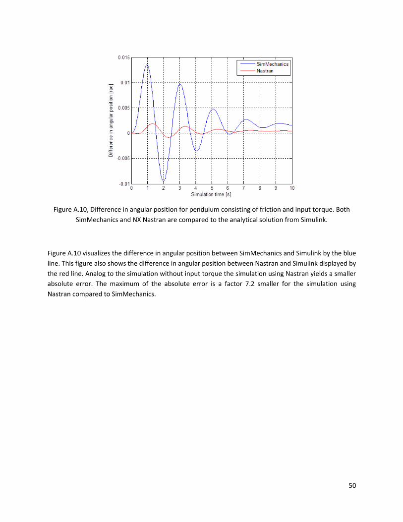
50
Figure A.10, Difference in angular position for pendulum consisting of friction and input torque. Both
SimMechanics and NX Nastran are compared to the analytical solution from Simulink.
Figure A.10 visualizes the difference in angular position between SimMechanics and Simulink by the blue
line. This figure also shows the difference in angular position between Nastran and Simulink displayed by
the red line. Analog to the simulation without input torque the simulation using Nastran yields a smaller
absolute error. The maximum of the absolute error is a factor 7.2 smaller for the simulation using
Nastran compared to SimMechanics.

51
References
[1] N. Takesue et al, High stiffness control of direct drive motor system by a homogenous ER fluid,
Proceedings of IEEE Int. Conf. Robotics and Automation, 1999
[2] National Instruments (2011), Motor Fundamentals, Retrieved 15-11-2013 from
http://www.ni.com/white-paper/3656/en/
[3] Matthew Burris, Stepper Motors vs Servo Motors – Selecting a Motor, Retrieved 15-11-2013 from
http://components.about.com/od/Components/a/Stepper-Motors-Vs-Servo-Motors-Selecting-A-
Motor.htm
[4] R. Siegwart, Introduction to autonomous mobile robots, pp. 31, The MIT Press, Massachusetts
Institute of Technology, Cambridge Massachusetts, 2004
[5] M. Rufli, Lecture Wheeled Locomotion lectured at 04-03-2013 from course Autonomous Mobile
Robots, ETH Zurich, Switzerland.
[6] M. Stania, R. Stetter, B. Poisadala, Dynamic Modeling of Wheeled Industrial Robots, 7th Workshop on
Advanced Control and Diagnosis, 19-20 November 2009, Zielone Gora, Polska
[7] Dragos George Calin (2013), Fundamental Guide for Stereo Vision Cameras in Robotics – Tutorials and
Resources, Retrieved 20-11-2013 from http://www.intorobotics.com/fundamental-guide-for-stereo-
vision-cameras-in-robotics-tutorials-and-resources/
[8] Pacejka, H.B., Tyre and Vehicle Dynamics, Oxford, Butterworth-Heineman, 2002
[9] NurulHuda Binti Muhamad Nasir, Mechanical Design of an Automated Guided Vehicle (AGV), Thesis
Bachelor of Manufacturing Engineering, National technical university college of Malaysia, 2005
[10] Farhan A. Salem, Dynamic and Kinematic Models and Control for Differential drive Mobile Robots,
International Journal of Current Engineering and Technology, vol. 3, no.2, pp. 253-263, June 2013
[11] Mehrdad Ehsani, Khwaja M. Rahman, Hamid A. Toliyat, Propulsion system design of electric and
hybrid vehicles, IEEE Trans. Ind. Electron., vol. 44, no. 1, 1997
[12] Khosro Bijanrostami, Design and Development of an Automated Guided Vehicle for Educational
Purposes, MSc. Thesis, Eastern Mediterranean University , Cyprus, September 2011
[13] Kristof Goris, Autonomous Mobile Robot Mechanical Design, MSc. Thesis, Vrije Universiteit Brussel,
Belgium, 2005
[14] Sisdarmanto Adinandra, Hierarchical coordination control of mobile robots, PhD Thesis, Eindhoven
University of Technology, Eindhoven, 2012

52
[15] Piero P. Bonissone, Kareem S. Aggour, Fuzzy Automated Braking System for Collision Prevention,
IEEE International Fuzzy Systems Conference, vol.3, pp. 757-760, 2001


