Simultaneous Siting and Sizing of Distribution Centers
on a Plane
Simin Huang∗, Rajan Batta∗∗ and Rakesh Nagi∗∗1
∗Department of Industrial Engineering, Tsinghua University, Beijing 100084,People’s Republic of China.
∗∗Department of Industrial Engineering, 342 Bell Hall,University at Buffalo (SUNY), Buffalo, NY 14260, USA.
Revised: September 2005December 2004
1For Correspondence: Email: [email protected], Tel: +1-716-645-2357x2103, Fax: +1-716-645-3302.

Abstract
The benefits of simultaneous consideration of siting and sizing of distribution centers have
been well acknowledged in supply chain design. Most formulations assume that the potential
DC sites are known and the decision on location is to select sites from the finite potential
DC sites. However, the quality of this discrete version problem depends on the selection of
potential DC sites. In this paper we present a planar version of the problem, which assumes
that there is no a priori knowledge of DC sites and DCs can be located anywhere in the
plane. The goal of the problem is to simultaneously find locations and sizing of DC sites.
The solution of the planar problem provides a lower bound for the discrete problem. The
objective of the problem is to minimize the total of inbound and outbound transportation
costs and distribution center construction costs – which include its fixed charge cost and
concave sizing cost. The problem is initially formulated as a nonlinear programming model.
We then reformulate it as a set covering problem after establishing certain key properties. A
greedy drop heuristic and a column generation heuristic are developed to solve the problem.
Computational experiments are provided.
Keywords: Distribution center sizing; Distribution center location; Supply chain design.
2
1 Introduction
This paper considers an integrated distribution center (DC) planar location and sizing prob-
lem in which products are shipped from plants to distribution centers (DCs) and then de-
livered to retailers. The objective of the problem is to minimize the total inbound and
outbound transportation costs and distribution center construction costs – which include its
fixed charge cost and concave sizing cost. Most formulations assume that the potential DC
sites are known and the decision on location is to select sites from the finite set of potential
DC sites. However, the quality of this discrete version problem depends on the selection of
potential DC sites. In this paper we assume that there is no a priori knowledge of DC sites
and DCs can be located anywhere on the plane. Therefore, the decision on location in this
problem is not to select but to generate DC sites. This version of the problem provides a
lower bound for the discrete problem. When the gap between the solutions of the discrete
and planar models is significant, it suggests that more potential DC sites should be added
in the candidate set of the discrete formulation. Another motivation of this paper is based
on the view that the design of such a system can be improved by simultaneous consideration
of location and sizing because of the trade-off between transportation costs and sizing costs.
However, the size issue in the planar location literature is neglected. In fact, Krarup and
Pruzan (1990) (page 41) point out that in most formulations reported in the literature, the
notion of facility size is essentially ignored and facilities are implicitly assumed to be points
in space as are the sites where they may be located.
The most related problem developed in the location literature is the planar location-
allocation problem, which was initiated in papers by Cooper (1963) and Cooper (1964). The
3

problem is to locate a set of p new facilities in a plane and assign a set of m existing facilities to
the new facilities in order to minimize total weighted distances. The main difficulty in solving
this problem arises from the fact that its objective function is neither convex nor concave
(see Cooper (1967)), and it is not differentiable everywhere. In general, it contains a large
number of local minima (see Eilon, Watson-Gandy, and Christofides (1971)). Therefore, most
models in this area assume that facilities are uncapacitated. Very few planar location models
consider the sizing issue. As far as we know, the only exception is the paper by Brimberg
and Love (1994). They consider a location-allocation problem with economies of scale and
present heuristic approaches to solve small-size problems. An overview of applications of
location-allocation problems is given in Hodgson, Rosing, and Shmulevitz (1993).
The other related problem is the facility sizing problem. It seeks to find a facility size
which allows a required service level to be attained and/or minimizes total costs. Facilities
can be broadly defined as buildings where people, material, and machines come together for
a stated purpose – typically to make a tangible product or provide a service (see Heragu
(1997)). Therefore, it is natural to classify the facility sizing problem based on its space
requirement, server number, inventory size, or machine capacity (or types). The warehouse
space requirement problem can be found in Sung and Han (1992), White and Francis (1971),
Lowe, Francis, and Reinhardt (1979) and Jucker, Carlson, and Kropp (1982). The server
allocation of queueing facilities has been studied in Brimberg, Mehrez, and Wesolowsky
(1997) and Brimberg and Mehrez (1997). For warehouse inventory sizing problem, Cormier
and Gunn (1996b) and Cormier and Gunn (1996a) coordinate warehouse size and inventory
policy under the assumption of constant product demand. In the case of deterministic facil-
ity capacity, Lee (1991) and Mazzola and Neebe (1999) study a multi-product capacitated
4

facility location problem with a choice of facility type. All of these models assume that either
facility locations are fixed or there is a priori knowledge of facility locations. Also, sizing
is a major issue in Huff Gravity models. A recent reference where sizing are optimized is
Aboolian, Berman, and Krass (2004).
This paper is organized as follows: Section 2 presents a mathematical formulation of the
problem and establishes properties of the model. Section 3 reformulates the model as a set
covering problem. A greedy drop heuristic and a column generation heuristic are developed
to solve it. Section 4 reports on computational results for both algorithms. Finally, Section
5 provides a summary and directions for future work.
2 Formulation
We are given a set of plant nodes, I = {1, 2, · · · , m}, and a set of retailer nodes, J =
{1, 2, · · · , n}. Let (i, j) denote a flow from plant i to retailer j and fij its flow amount,
∀ i ∈ I and j ∈ J . Let k ∈ K = {1, 2, · · · , p} be a DC index.
We assume that the transportation costs are determined by the distances of the shortest
paths between nodes. Let Yk be the location decision variable of DC k and d(i, Yk) be the
shortest distance between plant node i and DC k, where d(·) is a distance measure. Let xijk
be the fraction of flow amount fij that passes through DC k. Then, the transportation cost
can be expressed as
∑i∈I
∑j∈J
∑k∈K
fij(d(i, Yk) + d(Yk, j))xijk.
Generally speaking, DC sizing cost is based on its space requirement, server number,
inventory size, or machine capacity (or types), which should be determined by the maximum
5
flow amount that can go through the DC. Let ck be the sizing variable of DC k. We assume
that the sizing cost function of DC k, fk(c), includes its fixed charge cost and concave sizing
cost. It takes the form as follows:
F × I(ck) + h(ck), ∀ k ∈ K,
where F is a constant which denotes the fixed charge cost of a DC, I(ck) is an indicator
function with I(0) = 0 and I(ck > 0) = 1, and h(ck) is an increasing concave function of ck
and h(0) = 0.
The objective of the simultaneous DC siting and sizing problem is to minimize total of
inbound and outbound transportation costs and distribution center sizing costs. Then, the
problem can be formulated as follows:
(P ) minc, x, y
ZP (c, x, y) =∑i∈I
∑j∈J
∑k∈K
fij(d(i, Yk) + d(Yk, j))xijk
+∑k∈K
(F × I(ck) + h(ck)) (1)
subject to∑k∈K
xijk = 1, ∀ i ∈ I, j ∈ J, (2)
∑i∈I
∑j∈J
fijxijk ≤ ck, ∀ k ∈ K, (3)
xijk, ck ≥ 0, Yk ∈ R2 ∀ i ∈ I, j ∈ J, k ∈ K. (4)
The objective function (1) minimizes the total transportation cost and DC sizing cost.
Constraint (2) stipulates that the flows are only transported through DCs. Constraint (3)
is a capacity constraint. Constraints (4) are non-negativity constraints.
The major difficulty in solving this problem is due to the form of the objective function,
which is neither convex nor concave. We establish some properties with the hope of finding
6
an effective solution procedure for Problem (P ). For simplicity, we develop the properties
and a heuristic algorithm under the Manhattan distance. However, they can be extended to
the general polyhedral gauge case (see Huang, Batta, Klamroth, and Nagi (2005)).
In this paper, we consider the grid construction for the Manhattan distance as follows:
Consider the smallest rectangle (bounding rectangle) that encloses all plants and retailers
and whose sides are parallel to the x and y axes. Within this bounding rectangle, the grid
is formed by lines parallel to the x and y axes through all plant and retailer nodes. A grid
point is an intersection point of any two lines.
Property 1. There exists at least one optimal solution of Problem (P ) with the Manhattan
distance for which each DC is located on a grid point.
Proof: If all Y ∗k s are located at grid points, then we already obtain the property.
Suppose that the assertion is not true and let (c∗, x∗, y∗) be an optimal solution for
Problem (P ). If all Y ∗k s are located at grid points, then we already obtain the property. If
at least one of them is not located at a grid point, without loss generality, we assume that
Y ∗1 is not a grid point and located inside the rectangle ABCD (see Figure 1); here A, B, C,
and D are grid points and there are no grid points in the interior of rectangle ABCD. Let
RA, RB, RC , and RD be the northwestern region of node A, the northeastern region of node
B, the southwestern region of node C, and the southeastern region of node D, respectively.
We also assume that
∑i∈RA
∑j∈RC
fijx∗ij1 +
∑i∈RC
∑j∈RA
fijx∗ij1 ≥
∑i∈RB
∑j∈RD
fijx∗ij1 +
∑i∈RD
∑j∈RB
fijx∗ij1,
∑i∈RA
∑j∈RB
fijx∗ij1 +
∑i∈RB
∑j∈RA
fijx∗ij1 ≥
∑i∈RC
∑j∈RD
fijx∗ij1 +
∑i∈RD
∑j∈RC
fijx∗ij1.
Let ∆1 be the horizontal distance between Y ∗1 and A and ∆2 be the vertical distance
7

between Y ∗1 and A. Now, if we move Y ∗
1 to the grid point A and all others remain unchanged,
then the net improvement of the objective function value is
∆1
⎛⎝∑
i∈RA
∑j∈RC
fijx∗ij1 +
∑i∈RC
∑j∈RA
fijx∗ij1 −
∑i∈RB
∑j∈RD
fijx∗ij1 +
∑i∈RD
∑j∈RB
fijx∗ij1
⎞⎠
+∆2
⎛⎝∑
i∈RA
∑j∈RB
fijx∗ij1 +
∑i∈RB
∑j∈RA
fijx∗ij1 −
∑i∈RC
∑j∈RD
fijx∗ij1 +
∑i∈RD
∑j∈RC
fijx∗ij1
⎞⎠ ≥ 0.
Thus the objective function will not increase if we move Y ∗1 to a grid point. This procedure
can be repeated for any other Y ∗k which is not currently at a grid point. Thus a grid point
solution of equal or superior value can be constructed from any non-grid point solution. The
property follows.
*1Y
2
1
DC
BA
RR
RR
DC
BA
Figure 1: Proof of grid point optimality
Property 2. If (c∗, x∗, y∗) is an optimal solution for Problem (P ), then
c∗k =∑i∈I
∑j∈J
fijx∗ijk, ∀ k ∈ K.
Proof: Suppose that there exists an l ∈ K such that c∗l �= ∑i∈I
∑j∈J fijx
∗ijl. According
to constraint (3), c∗l >∑
i∈I
∑j∈J fijx
∗ijl. Let c
′l =
∑i∈I
∑j∈J fijx
∗ijl, then h(c∗l ) > h(c
′l)
(because h(·) is an increasing function). Using c′l to replace c∗l in the optimal solution, we
can claim that the new solution has a lower objective function value. The result follows by
contradiction.
8
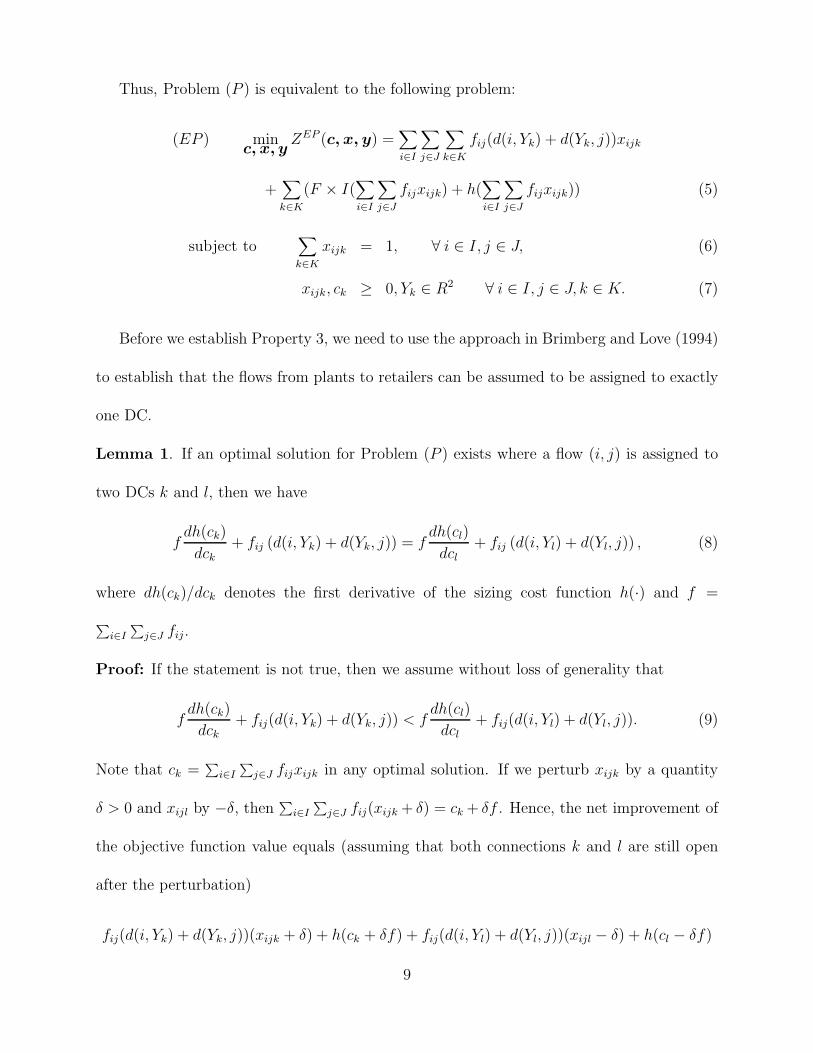
Thus, Problem (P ) is equivalent to the following problem:
(EP ) minc, x, y
ZEP (c, x, y) =∑i∈I
∑j∈J
∑k∈K
fij(d(i, Yk) + d(Yk, j))xijk
+∑k∈K
(F × I(∑i∈I
∑j∈J
fijxijk) + h(∑i∈I
∑j∈J
fijxijk)) (5)
subject to∑k∈K
xijk = 1, ∀ i ∈ I, j ∈ J, (6)
xijk, ck ≥ 0, Yk ∈ R2 ∀ i ∈ I, j ∈ J, k ∈ K. (7)
Before we establish Property 3, we need to use the approach in Brimberg and Love (1994)
to establish that the flows from plants to retailers can be assumed to be assigned to exactly
one DC.
Lemma 1. If an optimal solution for Problem (P ) exists where a flow (i, j) is assigned to
two DCs k and l, then we have
fdh(ck)
dck+ fij (d(i, Yk) + d(Yk, j)) = f
dh(cl)
dcl+ fij (d(i, Yl) + d(Yl, j)) , (8)
where dh(ck)/dck denotes the first derivative of the sizing cost function h(·) and f =
∑i∈I
∑j∈J fij.
Proof: If the statement is not true, then we assume without loss of generality that
fdh(ck)
dck+ fij(d(i, Yk) + d(Yk, j)) < f
dh(cl)
dcl+ fij(d(i, Yl) + d(Yl, j)). (9)
Note that ck =∑
i∈I
∑j∈J fijxijk in any optimal solution. If we perturb xijk by a quantity
δ > 0 and xijl by −δ, then∑
i∈I
∑j∈J fij(xijk + δ) = ck + δf . Hence, the net improvement of
the objective function value equals (assuming that both connections k and l are still open
after the perturbation)
fij(d(i, Yk) + d(Yk, j))(xijk + δ) + h(ck + δf) + fij(d(i, Yl) + d(Yl, j))(xijl − δ) + h(cl − δf)
9

−(fij(d(i, Yk) + d(Yk, j))xijk + h(ck) + fij(d(i, Yl) + d(Yl, j))xijl + h(cl))
= δ
(f
h(ck + δf) − h(ck)δf
+ fij(d(i, Yk) + d(Yk, j)) −(
fh(cl + δf) − h(cl)
δf+ fij(d(i, Yl) + d(Yl, j))
)).
Since dh(ck)/dck = limδf→0h(ck+δf)−h(ck)
δfand f is a constant, by (9), the net improvement
of the objective function value will be negative when δ → 0. The statement follows from the
ensuing contradiction.
Property 3. There exists an optimal solution of Problem (P ) for which each plant-retailer
flow (i, j) is allocated to a single DC, i.e., xijk = 0 or 1, ∀ i ∈ I, j ∈ J, k ∈ K, if h(·) is an
increasing concave function and ck is unbounded.
Proof: Suppose that there is an optimal solution for Problem (P ) with a flow (i, j) that is
allocated to at least two different DCs, say k and l. Then both xijk and xijl are positive.
Let us arbitrarily increase xijk by an amount δ = xijl and decrease xijl to zero. Since h(·) is
concave, we obtain,
h(ck + δf) − h(ck) ≤ δfdh(ck)
dck,
and
h(cl) − h(cl − δf) ≥ δfdh(cl)
dcl.
¿From the proof of Lemma 1, we know the net improvement of the objective function value
is
δ
(f
h(ck + δf) − h(ck)δf
+ fij(d(i, Yk) + d(Yk, j)) −(
fh(cl + δf) − h(cl)
δf+ fij(d(i, Yl) + d(Yl, j))
))
≤ δ
(f
dh(ck)
dck
+ fij(d(i, Yk) + d(Yk, j))
)− δ
(f
dh(cl)
dcl
+ fij(d(i, Yl) + d(Yl, j))
)= 0.
The last equation follows from Lemma 1. Thus, a new feasible solution is obtained which is
at least as good as the original optimal solution, and which has one less non-zero variable.
10
We repeat the process until each flow is completely allocated to its single DC. The result
follows.
If only a single DC needs to be located, by Property 2, the sizing cost term in Problem
(P ) is a constant in any optimal solution and constraint (3) is redundant. Therefore, the
problem becomes
(SP ) minc, y
ZSP (c, y) =∑i∈I
∑j∈J
∑k∈K
fij(d(i, Yk) + d(Yk, j)). (10)
Let all origin-destination nodes be the existing nodes. For each existing nodes, its demand
is either∑
j∈J fij (for origin node) or∑
i∈I fij (for destination node). Thus we obtain the
following property:
Property 4. If only a single DC needs to be located, Problem (P ) reduces to a standard
single facility location problem.
3 Set covering problem and column generation approach
In this section, we first reformulate Problem (P ) as a set covering problem. Then a column
generation approach is presented to solve the problem.
3.1 Set covering model
By Property 3, an optimal solution to Problem (P ) consists of a partition of origin-destination
flow (i, j) into nonempty subsets. We can find an optimal partition from all nonempty
subsets of the demand flow set by solving a set covering problem. Let S be the collection of
all nonempty subsets of the origin-destination flow set, i.e., S = {W1, W2, · · · , Ws, · · ·}. Let
11
bijs be a constant that is equal to 1 if origin-destination flow (i, j) is included in subset Ws
and 0 otherwise, and os,Ykbe the related total cost if Ws is assigned to a single DC located
at Yk. Thus,
os,Yk= F +
∑(i,j)∈Ws
fij(d(i, Yk) + d(Yk, j) + h
⎛⎝ ∑
(i,j)∈Ws
fij
⎞⎠ .
By Property 4, for a given Ws, locating the single DC can be reduced to a standard single
facility location problem. Suppose that T sYk
is the optimal transportation cost in the standard
single facility location problem for Ws, i.e.,
T sYk
= min∑
(i,j)∈Ws
fij(d(i, Yk) + d(Yk, j)),
and Ws is not empty, then we obtain the lowest cost of having one DC serve the flow set Ws,
os, as follows:
os = F + T sYk
+ h
⎛⎝ ∑
(i,j)∈Ws
fij
⎞⎠
= F + T sYk
+ h
⎛⎝∑
i∈I
∑j∈J
fijbijs
⎞⎠ .
Let decision variable zs = 1 if the origin-destination flow set Ws is selected to be served
by a DC and 0 otherwise. Problem (P ) or (EP ) can be reformulated into a set covering
problem as follows:
(SC) minz
ZSC(z) =∑
Ws∈Soszs (11)
subject to∑
Ws∈Sbijszs ≥ 1, ∀ i ∈ I, j ∈ J, (12)
zs ∈ {0, 1}, ∀ Ws ∈ S. (13)
Constraint (12) guarantees that each origin-destination flow belongs to at least one selected
origin-destination flow set. Constraint (13) is the integrality constraint. For this set covering
problem, we obtain the following property:
12

Property 5. There is no optimal solution for Problem (SC) such that Ws and Ws′ are
assigned to the same DC, where Ws and Ws′ are any two origin-destination flow sets.
Proof: Suppose that there is an optimal solution for Problem (SC) such that Ws and Ws′
are assigned to the same DC k with location Yk. According to the definition of os, we obtain,
os + os′ = F + T sYk
+ h
⎛⎝∑
i∈I
∑j∈J
fijbijs
⎞⎠
+F + T s′Yk
+ h
⎛⎝∑
i∈I
∑j∈J
fijbijs′
⎞⎠ .
Let Wu = Ws ∪ Ws′ , assign Wu to DC k and drop Ws and Ws
′ . Then the related cost
becomes,
ou = F + T sYk
+ T s′Yk
+ h
⎛⎝∑
i∈I
∑j∈J
fijbijs +∑i∈I
∑j∈J
fijbijs′
⎞⎠ .
Since h(x) + h(y) ≥ h(x + y), for any x ≥ 0 and y ≥ 0 (because h is concave), it is easy
to see that ou ≤ os + os′ . By doing this and keeping everything else unchanged, we obtain a
new feasible solution, which is at least as good as the old one. The result follows.
This property guarantees that only one origin-destination flow set will be assigned to
each generated DC in the optimal solution.
The number of columns involved in this formulation is exponential. Neither the set
covering problem nor its linear programming relaxation can be solved by a method that
first generates all feasible columns explicitly. We therefore resort to a column generation
approach.
13

3.2 Column generation approach
Let (S̄C) be the linear programming relaxation of (SC) and (S̄CS′ ) be the master problem
of (S̄C) in which a subset S ′of S is available. Thus, the master problem (S̄CS′ ) is as follows:
(S̄CS′ ) minz
Z S̄CS′ (z) =∑
Ws∈S′oszs (14)
subject to∑
Ws∈S′bijszs ≥ 1, ∀ i ∈ I, j ∈ J, (15)
0 ≤ zs ≤ 1 ∀ Ws ∈ S ′. (16)
From the theory of linear programming, we know that a solution to a minimization
problem is optimal if the reduced cost of each variable is nonnegative. Here, the reduced
cost o∗s of any subset Ws is given by
o∗s = os −∑i∈I
∑j∈J
λijbijs
= F + T sYk
+ h
⎛⎝∑
i∈I
∑j∈J
fijbijs
⎞⎠−∑
i∈I
∑j∈J
λijbijs,
where λij is the given value of the dual variable corresponding to constraint (15) for i and
j. To test whether the current solution is optimal, we determine if there exists a Ws with
negative reduced cost. Thus the pricing problem is as follows:
(PP ) min∑i∈I
∑j∈J
fij(d(i, Yk) + d(Yk, j))xijk + h
⎛⎝∑
i∈I
∑j∈J
fijxijk
⎞⎠−∑
i∈I
∑j∈J
λijxijk, (17)
subject to xijk ∈ {0, 1}, Yk ∈ R2, ∀ i ∈ I, j ∈ J, k ∈ K. (18)
Here, we drop the constant F and will add it to the optimal objective function value after the
pricing problem is solved. The pricing problem is a mixed integer nonlinear programming
14

problem. The difficulty to solve this problem is two fold. First, the DC location Yk is a
variable. Therefore,∑
i∈I
∑j∈J fij(d(i, Yk) + d(Yk, j))xijk is a mixed integer nonlinear term.
Second, the function h(·) is a concave function. However, according to Property 1, we know
that DCs will be located at grid points in an optimal solution. Thus, we choose the DC
locations from the grid points. For given grid point,∑
i∈I
∑j∈J fij(d(i, Yk)+d(Yk, j))xijk is a
linear function of xijk. If for every grid point we have nonnegative reduced cost, then every
subset Ws has nonnegative reduced cost. Let G be the set of all grid points. The pricing
problem reduces to the following problem (RPPk) for each grid point Yk ∈ G:
(RPPk) minx
ZRPPk(x) =∑i∈I
∑j∈J
(fijdijk − λij)xijk + h
⎛⎝∑
i∈I
∑j∈J
fijxijk
⎞⎠ , (19)
subject to xijk ∈ {0, 1}, ∀ i ∈ I, j ∈ J, (20)
where dijk = d(i, Yk)+d(Yk, j) is a known constant here since Yk is a grid point. Coincidently,
the pricing problem is very similar to the one in Shen, Coullard, and Daskin (2003). They
developed an effective approach to solve such the pricing problem. Following their idea, we
can develop an algorithm to solve the pricing problems in polynomial time.
Let x∗ be an optimal solution to Problem (RPPk) and the minimum reduced-cost set
Ws = {(i, j) : x∗ijk = 1}, and G∗
k = F + ZRPPk(x∗). If G∗k ≥ 0, then we can conclude that
there is no set Ws assigning to grid point k with negative reduced cost. If ∀k, G∗k ≥ 0, we
can conclude that there is no set Ws ∈ S with negative reduced cost.
Now suppose that all flows (i, j), ∀ i ∈ I, j ∈ J , have been sorted so that:
fi1j1di1j1k − λi1j1
fi1j1
≤ fi2j2di2j2k − λi2j2
fi2j2
≤ · · · ≤ fiγjγdiγjγk − λiγjγ
fiγjγ
,
15

where γ is the total number of non-zero flows. Then, the following theorem is an immediate
consequence from Shen, Coullard, and Daskin (2003).
Theorem 1. There is an optimal solution x∗ijk to Problem (RPPk) in which the following
properties hold:
1. If fijdijk ≥ λij, then x∗ijk = 0, ∀ i ∈ I, j ∈ J .
2. If x∗itjtk = 1, for some t ∈ {1, 2, · · · , γ}, then x∗
iljlk= 1, for all l ∈ {1, 2, · · · , t − 1}.
Using Theorem 1, we can develop an algorithm to solve the pricing problems in poly-
nomial time. In fact, we can solve Problem (RPPk) by enumeration, i.e., by generating all
solutions with the properties and selecting the one with the lowest objective function value.
The complexity of the pricing problem is O((m + n)2mn log(mn)), where m and n are total
numbers of plant and retailer nodes, respectively.
3.3 Greedy drop heuristic algorithm
In this section we develop a greedy drop heuristic algorithm to solve Problem (P ). The
purpose of this section is twofold. First, we need a set of initial columns. Second, we need
a good upper bound. Both objectives can be achieved by using a greedy drop heuristic
algorithm. To present this algorithm we first need to introduce the concept of a shortest
path flow set.
3.3.1 The shortest path flow set
Before we develop the heuristic algorithm, we need to introduce a shortest path flow set of
each grid point for a given grid construction. The grid construction under the Manhattan
16

distance in this paper is defined in Section 2.
We define the shortest path flow set for each grid point as follows. Let (i, j) refer to a pair
of plant and retailer with coordinates (xi, yi) and (xj , yj), respectively, and s refer to any
grid point with location coordinates (xs, ys). Then the shortest path flow set of grid point s,
Ps, is given by:
Ps := {(i, j) : xi ≤ xs, yi ≥ ys, xj ≥ xs, yj ≤ ys} ∪ {(i, j) : xi ≤ xs, yi ≤ ys, xj ≥ xs, yj ≥ ys}
∪{(i, j) : xi ≥ xs, yi ≥ ys, xj ≤ xs, yj ≤ ys} ∪ {(i, j) : xi ≥ xs, yi ≤ ys, xj ≤ xs, yj ≥ ys}.
Under the Manhattan distance, if we select s as a DC location, then for all (i, j) ∈ Ps the
shortest path from plant i to retailer j passes through s. Figure 2 provides examples of sets
Ps.
, ()2, j1{(i=sP
Grid PointPlantRetailer
i
j
i
j
i1
2
)}22 , ji)1 , (, j2
4
j
j 1
2
s
3
Figure 2: An illustration of the shortest path flow set
17

3.3.2 Greedy drop heuristic algorithm
The greedy drop heuristic algorithm is built based on the shortest path flow set of each grid
point. Let fs =∑
(i,j)∈Psfij . Then fs is the total flow amount that passes through s with
the shortest distance. Intuitively, the larger fs is, the more important the grid point s is
because of the concave sizing cost function. Thus, the basic idea for this heuristic algorithm
is to use the order of fs to find a heuristic solution.
The greedy drop heuristic algorithm is as follows: First, we define W to be the set of all
plant-retailer pairs, (i, j), ∀ i ∈ I, j ∈ J , and W u to be the set of (i, j) that are currently
not assigned to any DC. Initialize G = {s : s is a grid point} and W u := W . Find the
shortest path flow set, fs =∑
(i,j)∈Ps∩W u fij , ∀s ∈ G. Pick the grid point s with the largest
fs value as a candidate DC location and assign all (i, j) ∈ Ps ∩ W u to this DC, and let
Ws = {(i, j) ∈ Ps ∩ W u}. Update W u := W u \ Ps and G := G \ {s}, and repeat the
procedure until W u is empty. Using this procedure, we obtain a collection of initial Ws sets
and their corresponding grid points.
Second, we drop one initial Ws, assign the flows of this set to the nearest available
grid point that is selected above, and recalculate the objective function. The procedure is
repeated for all initial Ws sets. Then we drop the Ws with the most improved objective
function, update Ws and repeat the procedure until we see no further improvement in the
objective function value.
Each step of the algorithm generates a collection of Ws sets. All of them could be used
as an initial subset S ′in the column generation algorithm. We also note that the solution of
the greedy drop heuristic algorithm provides an upper bound for the original problem (P ).
18

3.4 Column generation algorithm
Now, we are ready to give a step-wise description of the column generation algorithm as
follows:
1. Generate the initial subset S ′as described above.
2. Solve the linear programming relaxation to obtain the vector of current dual costs.
3. Use the pricing algorithm to determine if there is subset Ws whose associate column
has negative reduced cost. If such subset Ws exist, then add it to S ′and go to step 2.
4. If no such subset Ws exist, then stop. Solve the set covering problem (SC) for S ′.
4 Computational Results
In this section, we test the performance of the greedy drop heuristic algorithm and the
column generation algorithm. The efficiency of the algorithms are tested by solving randomly
generated problems of different sizes. The algorithms were programmed in Microsoft Visual
C++ 5.0 and CPLEX8.1. All of the experimental tests were carried out on a Dell OptiPlex
GX240 with 512MB RAM and 1.8GHz CPU. Computation times are in seconds.
4.1 Data generation
First, we generated locations of each plant and retailer, which are given by their x and
y coordinates. These coordinate values were randomly selected from U(0, 200), where U
denotes a uniform distribution. For each pair of plant-retailer, the amount of flow was
19

randomly drawn from U(5, 30). The constant fixed charge cost of a DC, F , was 1000.
Also, the DC sizing cost function was set to be h(ck) = 50√
ck. The sizes of randomly
generated problems were the combination of the following parameters: number of plant
nodes m = 5, 10; number of retailer nodes n = 10, 15, 20, 25, 30; and total number of flows
from plants to retailers were 50, 60, 70, 80, 90, 100.
4.2 Computational performance
Here we report the performance of the greedy drop heuristic algorithm and the column
generation algorithm for Problem (P ).
We had two schemes for adding the negative reduced cost column to the linear program
after having solved the pricing algorithm. In the first one (called Cg1 ), we iteratively added
a column with the smallest negative reduced cost from all k ∈ G to the linear program. We
continued the procedure until the pricing problems could not find a negative reduced cost
column, i.e., the linear programming relaxation problem was solved optimally. In the second
scheme (called Cg2 ), we remove some columns during the column generation procedure so
as to reduce the size of the restricted master problem. The criterion of removing a column
is as follows: calculate the average reduced cost for the existing columns that have positive
reduced costs, then remove those columns whose reduced cost is greater than or equal to
two times of the average reduced cost.
Table 1 summarizes the computational results for the greedy drop heuristic algorithm
and the column generation algorithms (both Cg1 and Cg2 ). Some headers of the columns
in Table 1 are:
20
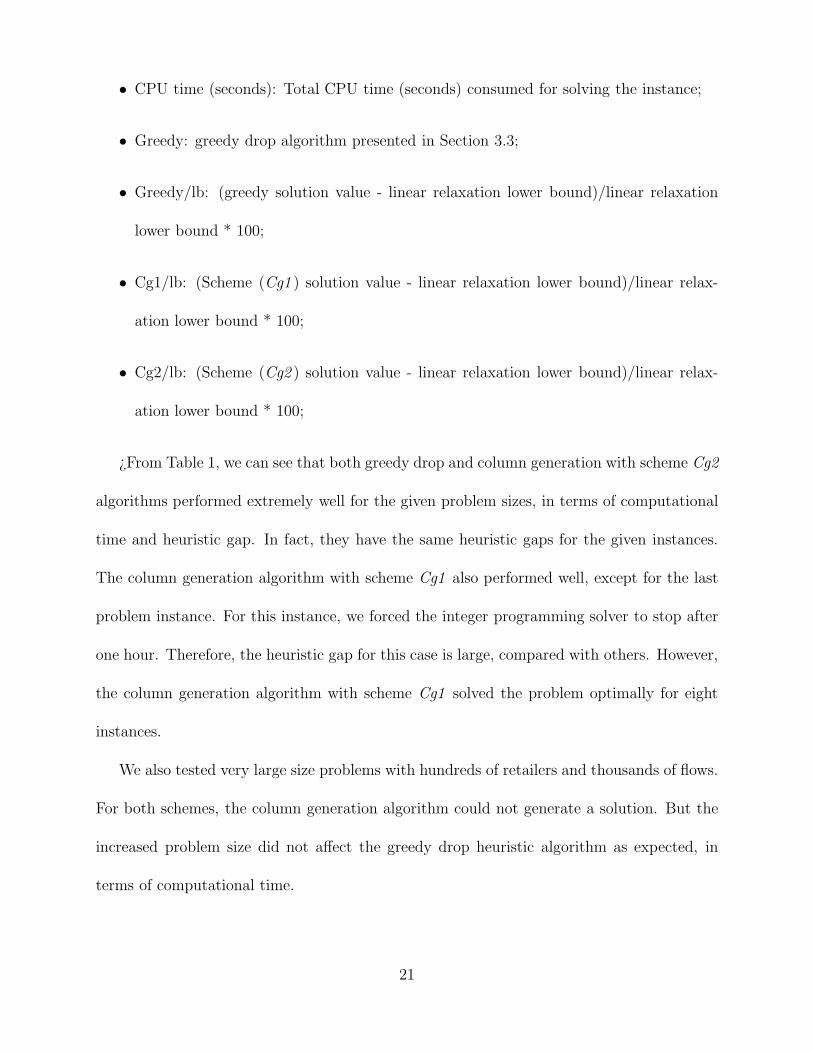
• CPU time (seconds): Total CPU time (seconds) consumed for solving the instance;
• Greedy: greedy drop algorithm presented in Section 3.3;
• Greedy/lb: (greedy solution value - linear relaxation lower bound)/linear relaxation
lower bound * 100;
• Cg1/lb: (Scheme (Cg1 ) solution value - linear relaxation lower bound)/linear relax-
ation lower bound * 100;
• Cg2/lb: (Scheme (Cg2 ) solution value - linear relaxation lower bound)/linear relax-
ation lower bound * 100;
¿From Table 1, we can see that both greedy drop and column generation with scheme Cg2
algorithms performed extremely well for the given problem sizes, in terms of computational
time and heuristic gap. In fact, they have the same heuristic gaps for the given instances.
The column generation algorithm with scheme Cg1 also performed well, except for the last
problem instance. For this instance, we forced the integer programming solver to stop after
one hour. Therefore, the heuristic gap for this case is large, compared with others. However,
the column generation algorithm with scheme Cg1 solved the problem optimally for eight
instances.
We also tested very large size problems with hundreds of retailers and thousands of flows.
For both schemes, the column generation algorithm could not generate a solution. But the
increased problem size did not affect the greedy drop heuristic algorithm as expected, in
terms of computational time.
21
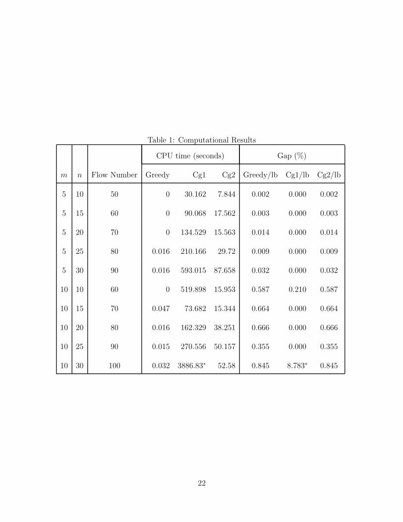
Table 1: Computational Results
CPU time (seconds) Gap (%)
m n Flow Number Greedy Cg1 Cg2 Greedy/lb Cg1/lb Cg2/lb
5 10 50 0 30.162 7.844 0.002 0.000 0.002
5 15 60 0 90.068 17.562 0.003 0.000 0.003
5 20 70 0 134.529 15.563 0.014 0.000 0.014
5 25 80 0.016 210.166 29.72 0.009 0.000 0.009
5 30 90 0.016 593.015 87.658 0.032 0.000 0.032
10 10 60 0 519.898 15.953 0.587 0.210 0.587
10 15 70 0.047 73.682 15.344 0.664 0.000 0.664
10 20 80 0.016 162.329 38.251 0.666 0.000 0.666
10 25 90 0.015 270.556 50.157 0.355 0.000 0.355
10 30 100 0.032 3886.83∗ 52.58 0.845 8.783∗ 0.845
22

5 Conclusion
This paper proposes a model for studying the problem of simultaneous consideration of
siting and sizing of DCs on the plane. The problem minimizes the total transportation cost
and DC sizing costs, which include its fixed charge cost and concave sizing cost. The most
significant results are the grid node optimality property under the Manhattan distance and
full flow assignment property under the concave sizing cost assumption. These results allow
us to reformulate the problem as a set covering problem and develop an efficient greedy drop
heuristic algorithm and a column generation heuristic algorithm. The computational results
show the efficiency and accuracy of the algorithms.
Several extensions of the problem are possible. For example, we assume that the fixed
charge sizing cost of a DC is constant for all potential DC sites. Developing a model for
location related fixed charge sizing cost is a possible topic for further research. The problem
could also be investigated under different distance measures, for example, the Euclidean
distance. The solution approach developed in this paper can also be extended to network
location and sizing problem, where DCs have to be located on a given network.
Acknowledgments
The authors would like to acknowledge support from the National Science Foundation via
Grant No. DMI-0300370. They would also like to thank the referees for their constructive
comments.
23
References
Aboolian, R., O. Berman, and D. Krass (2004). Competitive facilities location and design
problems on a network. Presented at the EURO XX Conference in Rhodes, Greece,
July 2004 .
Brimberg, J. and R. F. Love (1994). A location problem with economies of scale. Studies
in Locational Analysis 7, 9–19.
Brimberg, J. and A. Mehrez (1997). A note on the allocation of queueing facilities using
a minisum criterion. Journal of the Operational Research Society 48, 195–201.
Brimberg, J., A. Mehrez, and G. O. Wesolowsky (1997). Allocation of queueing facilities
using a minimax criterion. Location Science 5, 89–101.
Cooper, L. (1963). Location-allocation problems. Operations Research 11, 331–343.
Cooper, L. (1964). Heuristic methods for location-allocation problems. SIAM Review 6,
37–53.
Cooper, L. (1967). Solutions of generalized locational equilibrium models. Journal of Re-
gional Science 7, 1–18.
Cormier, G. and E. A. Gunn (1996a). On the coordination of warehouse sizing, leasing
and inventory policy. IIE Transactions 28, 149–154.
Cormier, G. and E. A. Gunn (1996b). Simple models and insights for warehouse sizing.
Journal of the Operational Research Society 47, 690–696.
Eilon, S., C. D. T. Watson-Gandy, and N. Christofides (1971). Distribution Management:
Mathematical Modelling and Practical Analysis. Hafner, New York.
24
Heragu, S. (1997). Facilities Design. PWS Publishing Company.
Hodgson, M. J., K. E. Rosing, and F. Shmulevitz (1993). A review of location-allocation
applications literature. Studies in Locational Analysis 5, 2–29.
Huang, S., R. Batta, K. Klamroth, and R. Nagi (2005). The K-connection location prob-
lem in a plane. Annals of Operations Research 136, 193–209.
Jucker, J. V., R. C. Carlson, and D. H. Kropp (1982). The simultaneous determination
of plant and leased warehouse capacities for a firm facing uncertain demand in several
regions. IIE Transactions 14, 99–108.
Krarup, J. and P. M. Pruzan (1990). Ingredients of locational analysis. In P. B. Mirchan-
dani and R. L. Francis (Eds.), Discrete Location Theory, pp. 1–54. John Wiley, New
York.
Lee, C. Y. (1991). An optimal algorithm for the multiproduct capacitated facility location
problem with a choice of facility type. Computers and Operations Research 20, 527–
540.
Lowe, T. J., R. L. Francis, and E. W. Reinhardt (1979). A greedy network flow algorithm
for a warehouse leasing problem. AIIE Transactions 11, 170–182.
Mazzola, J. B. and A. W. Neebe (1999). Lagrangian-relaxation-based solution procedures
for a multiproduct capacitated facility location problem with choice of facility type.
European Journal of Operational Research 115, 285–299.
Shen, Z. M., C. Coullard, and M. S. Daskin (2003). A joint location-inventory model.
Transportation Science 37, 40–55.
25

Sung, C. S. and Y. H. Han (1992). Determination of automated storage/retrieval system
size. Engineering Optimization 19, 269–286.
White, J. A. and R. L. Francis (1971). Normative models for some warehouse sizing
problems. AIIE Transactions 3, 185–190.
26


