
SINGLE PHOTONS FOR QUANTUM INFORMATION
PROCESSING
A DISSERTATION
SUBMITTED TO THE DEPARTMENT OF PHYSICS
AND THE COMMITTEE ON GRADUATE STUDIES
OF STANFORD UNIVERSITY
IN PARTIAL FULFILLMENT OF THE REQUIREMENTS
FOR THE DEGREE OF
DOCTOR OF PHILOSOPHY
David Fattal
September 2010

c© Copyright by David Fattal 2010
All Rights Reserved
ii
I certify that I have read this dissertation and that, in my opinion, it
is fully adequate in scope and quality as a dissertation for the degree
of Doctor of Philosophy.
Prof. Yoshihisa Yamamoto Principal Adviser
I certify that I have read this dissertation and that, in my opinion, it
is fully adequate in scope and quality as a dissertation for the degree
of Doctor of Philosophy.
Prof. Jelena Vuckovic
I certify that I have read this dissertation and that, in my opinion, it
is fully adequate in scope and quality as a dissertation for the degree
of Doctor of Philosophy.
Prof. Mark Kasevich
Approved for the University Committee on Graduate Studies.
iii

iv

Abstract
Single photons are attractive carriers of Quantum Information. Once produced, they
can be reliably manipulated and can travel long distances unaffected. They are the
main constituents of quantum communication protocols, and it is likely that they will
even play a major role in the development of quantum computers.
This work presents experimental and theoretical improvements of existing semi-
conductor quantum dot single photon sources for their application to quantum infor-
mation. We demonstrate the experimental realization of some basic optical quantum
information protocols: entanglement generation and quantum state teleportation.
We also develop fabrication and optical characterization techniques for a new type of
quantum dot based single photon source, with photonic crystal technology.
Aware of some intrinsic limitations of existing single photon sources, we go on to
develop an extensive theory for the coherent control of a single photon pulse using
cavity a QED technique. We show how to trap or generate a single photon pulse
reversibly in an atom-cavity system under the most general experimental conditions.
In particular we show how to realize such processes in a non-adiabatic way and in the
cavity QED regime of weak coupling. This technique allows the complete control over
a single photon pulse temporal amplitude, and gives the possibility of fast exchange
of quantum information in quantum networks. Relying on this technique, we explain
how to build the main elements of an all-integrated on-chip quantum computer based
on single QD electron spin and single photon exchange via photonic crystal cavities
and wave-guides.
v

Acknowledgements
The work performed during my graduate student years at Stanford was the result of
many collaborations, and was stimulated by uncountable hours of discussions with
Stanford students and faculty members. I would like to thank in particular my advisor
Pr. Yamamoto for his unbreakable enthusiasm regarding quantum science research,
and the freedom that he left me while doing research in his group. Every single
discussion I had with him was valuable in terms of new ideas and renewed scientific
excitement. I would like to thank Jelena Vuckovic with whom I performed work on
micropillar cavities, and who later on introduced me to the field of photonic crystals,
letting me work as part of her own group in the quantum dot - photonic crystal cavity
project. I want to thank Charles Santori for his guidance as I was a new student in
the group, and in general for his numerous pieces of advice inside and outside of the
lab.
I would like to express my thanks to my oral and reading thesis committee mem-
bers, Prof. Moerner, Kasevich, Vuckovic and Yamamoto, and Ray Beausoleil (who
in addition will have to put up with me in the next years at HP labs).
I want to acknowledge my direct collaborators in the lab, Kyo Inoue, Eleni Dia-
manti and her infallible smile, Edo Waks and Dirk Englund with whom I had the
sincere pleasure to work in my last years in a particularly friendly atmosphere. I had
the chance to share lab time or conversations with other members from the Yamamoto
and Vuckovic group, in particular Will Oliver, Matthew Pelton, Gregor Weihs, Cyrus
vi

Master, Thaddeus Ladd, Johnathan Goldman, Na Young Kim, Kai-Mei Fu, Ilya Fush-
man, Hatice Altug and Stephan Goetzinger. Outside from these groups, my learning
of nano-fabrication was greatly facilitated by James Conway who trained me on the
Raith e-beam lithography system and Luigi Scaccabarozzi who shared with me many
tips on photonic crystal fabrication. I also want to thank to Yurika Peterman for her
time and help in many occasions regarding everyday matters of my graduate student
life.
I was also fortunate to meet great people outside of Stanford. In particular I
want to thank Ike Chuang for his mentoring role and for sharing insights on quantum
information theory in many occasions. I want to thank as well Toby ’qubit’ Cubitt
and Sergey Bravyi for many stimulating discussions and their participation in our
theoretical work on the stabilizer formalism that I decided not to include in this the-
sis. I enjoyed valuable discussions with many other researchers who influenced my
work, including Serge Haroche, Jean Dalibard, Philippe Grangier, Sylvain Schwartz,
Gerard Rempe, Reinhard Blatt, Keiji Matsumoto, Kae Nemoto, Bill Munro, Steve
Harris, Barry Sanders, John Preskill, Guifre Vidal among others.
Finally I want to thank my parents Michele and Soly and my brother Bruno for
their support. I have a special thought for my dad who undoubtedly stimulated my
interest for science in general and physics in particular.
vii

viii

Science is Light...
ix

Contents
Abstract v
Acknowledgements vi
viii
1 Introduction 1
1.1 Quantum information theory . . . . . . . . . . . . . . . . . . . . . . . 2
1.1.1 Why is quantum powerful ? . . . . . . . . . . . . . . . . . . . 2
1.1.2 Physical processes required for QIP ? . . . . . . . . . . . . . . 4
1.2 Photonic approach to quantum information . . . . . . . . . . . . . . 5
1.2.1 Encoding quantum information in photons . . . . . . . . . . . 6
1.2.2 A wave-function for single photons ? . . . . . . . . . . . . . . 8
1.3 Summary of thesis . . . . . . . . . . . . . . . . . . . . . . . . . . . . 12
2 Single Photon source: Operation principle 13
2.1 Quantum Dots . . . . . . . . . . . . . . . . . . . . . . . . . . . . . . 13
2.1.1 Basic notions . . . . . . . . . . . . . . . . . . . . . . . . . . . 13
2.1.2 Fabrication method . . . . . . . . . . . . . . . . . . . . . . . . 15
2.1.3 Optical excitation methods . . . . . . . . . . . . . . . . . . . . 15
2.2 Optical micro-cavities . . . . . . . . . . . . . . . . . . . . . . . . . . . 17
2.2.1 Micropillar cavities . . . . . . . . . . . . . . . . . . . . . . . . 18
2.2.2 Photonic bandgap cavities . . . . . . . . . . . . . . . . . . . . 19
2.3 Single photon generation . . . . . . . . . . . . . . . . . . . . . . . . . 22
x
2.3.1 Temperature tuning . . . . . . . . . . . . . . . . . . . . . . . 22
2.3.2 Quantum efficiency . . . . . . . . . . . . . . . . . . . . . . . . 23
2.3.3 Degree of anti-bunching . . . . . . . . . . . . . . . . . . . . . 25
2.3.4 Quantum indistinguishability . . . . . . . . . . . . . . . . . . 25
3 Entanglement formation 30
3.1 Description of experiment . . . . . . . . . . . . . . . . . . . . . . . . 30
3.1.1 Background . . . . . . . . . . . . . . . . . . . . . . . . . . . . 30
3.1.2 Entanglement formation principle . . . . . . . . . . . . . . . . 31
3.1.3 Method . . . . . . . . . . . . . . . . . . . . . . . . . . . . . . 33
3.2 Results . . . . . . . . . . . . . . . . . . . . . . . . . . . . . . . . . . . 36
3.2.1 Bell inequality test . . . . . . . . . . . . . . . . . . . . . . . . 36
3.2.2 Quantum state tomography . . . . . . . . . . . . . . . . . . . 37
3.2.3 Discussion . . . . . . . . . . . . . . . . . . . . . . . . . . . . . 39
4 Single Mode Teleportation 42
4.1 Description of experiment . . . . . . . . . . . . . . . . . . . . . . . . 42
4.1.1 Background . . . . . . . . . . . . . . . . . . . . . . . . . . . . 42
4.1.2 Single-mode teleportation principle . . . . . . . . . . . . . . . 44
4.1.3 Method . . . . . . . . . . . . . . . . . . . . . . . . . . . . . . 46
4.2 Results . . . . . . . . . . . . . . . . . . . . . . . . . . . . . . . . . . . 48
4.2.1 Test of coherence transfer . . . . . . . . . . . . . . . . . . . . 48
4.2.2 Discussion . . . . . . . . . . . . . . . . . . . . . . . . . . . . . 50
5 Theory of coherent single photon emission and trapping 53
5.1 Background . . . . . . . . . . . . . . . . . . . . . . . . . . . . . . . . 53
5.2 Summary of results . . . . . . . . . . . . . . . . . . . . . . . . . . . . 55
5.2.1 General theory . . . . . . . . . . . . . . . . . . . . . . . . . . 55
5.2.2 Real systems: performance analysis . . . . . . . . . . . . . . . 60
5.3 Applications . . . . . . . . . . . . . . . . . . . . . . . . . . . . . . . . 64
5.3.1 Single photon generation . . . . . . . . . . . . . . . . . . . . 64
5.3.2 Non-destructive single photon detection . . . . . . . . . . . . . 66
xi

5.3.3 Formation of quantum entanglement between nodes . . . . . . 66
5.3.4 Non-destructive parity measurement for two nodes . . . . . . 66
5.3.5 Bell-state measurement for two nodes . . . . . . . . . . . . . . 67
5.3.6 Non-linear interaction of single photons . . . . . . . . . . . . . 69
5.3.7 Full QIP with electronic qubits . . . . . . . . . . . . . . . . . 69
5.3.8 Discussion . . . . . . . . . . . . . . . . . . . . . . . . . . . . . 70
5.4 Mathematical details of the theory. . . . . . . . . . . . . . . . . . . . 72
5.4.1 System dynamics . . . . . . . . . . . . . . . . . . . . . . . . . 72
5.4.2 Impedance matching . . . . . . . . . . . . . . . . . . . . . . . 74
5.4.3 Control pulse design . . . . . . . . . . . . . . . . . . . . . . . 76
5.4.4 Reflection of a single photon pulse off a passive node . . . . . 79
6 Conclusion and prospects 81
A Theory of Quantum Dot-cavity coupling 84
Bibliography 92
xii

List of Tables
3.1 Normalized coincidence counts for various polarizer angles used in the
Bell Inequality test. . . . . . . . . . . . . . . . . . . . . . . . . . . . . 37
xiii

List of Figures
1.1 Qualitative difference between a single photon pulse and a weak laser
pulse. . . . . . . . . . . . . . . . . . . . . . . . . . . . . . . . . . . . . 6
2.1 Spatial variation of conduction and valence band energies in a QD. . 14
2.2 Above-band excitation technique. . . . . . . . . . . . . . . . . . . . . 16
2.3 Resonant excitation of a QD. . . . . . . . . . . . . . . . . . . . . . . 17
2.4 Photoluminescence spectra of a single QD under above-band or reso-
nant excitation. . . . . . . . . . . . . . . . . . . . . . . . . . . . . . . 18
2.5 Micropillar cavities used in the QIP experiments of this work. . . . . 19
2.6 SEM pictures of photonic crystal membranes fabricated during the thesis. 20
2.7 Single photon source characterization setup used with micropillar sam-
ples. With PBG samples, a confocal microscope setup was preferred to
the side excitation shown here , so that a narrow region (submicron)
only could be illuminated. . . . . . . . . . . . . . . . . . . . . . . . . 23
2.8 Measured spontaneous emission rate of a QD exciton in a micropillar
cavity, as a function of its detuning from the cavity resonance. The
dot emission wavelength is tuned by changing the sample temperature
within the 6 K - 40 K range. . . . . . . . . . . . . . . . . . . . . . . . 24
2.9 Intensity auto-correlation histogram. g(2)(0) is given by the ratio of
coincidence counts in the ”central” peak and in a ”side” peak. . . . . 26
2.10 Mandel-type setup used to perform a photon bunching experiment and
measure the overlap of photons emitted consecutively in a SPS. . . . 28
xiv

2.11 Correlation histogram resulting from a photon bunching experiment.
The overlap of consecutive photons can be inferred from the depth of
the central dip. . . . . . . . . . . . . . . . . . . . . . . . . . . . . . . 28
3.1 Experimental setup. . . . . . . . . . . . . . . . . . . . . . . . . . . . 34
3.2 Zoom on a typical correlation histogram,... . . . . . . . . . . . . . . . 35
3.3 Reconstructed polarization density matrix for the post-selected photon
pairs... . . . . . . . . . . . . . . . . . . . . . . . . . . . . . . . . . . . 38
4.1 Schematic of single mode teleportation. . . . . . . . . . . . . . . . . . 46
4.2 Experimental setup. . . . . . . . . . . . . . . . . . . . . . . . . . . . 47
4.3 Typical correlation histograms . . . . . . . . . . . . . . . . . . . . . . 49
4.4 Verification of single mode teleportation. . . . . . . . . . . . . . . . . 51
5.1 Simulation of a high Q micro-cavity coupled to a single waveguide
transverse mode realized in a 2D photonic crystal. . . . . . . . . . . . 55
5.2 Composition of a ”node”: 3-level atom or quantum dot in a Λ config-
uration placed in a single mode optical micro-cavity. . . . . . . . . . . 57
5.3 Physical picture of the photon trapping process. . . . . . . . . . . . . 58
5.4 Control pulse Ω(t) to apply to trap a single photon pulse of given
amplitude α(t). . . . . . . . . . . . . . . . . . . . . . . . . . . . . . . 61
5.5 Generation and trapping of a single photon pulse with oscillating am-
plitude. . . . . . . . . . . . . . . . . . . . . . . . . . . . . . . . . . . 62
5.6 Deterministic photon trapping/generation deep in the weak coupling
regime. . . . . . . . . . . . . . . . . . . . . . . . . . . . . . . . . . . . 63
5.7 Generation and trapping of a composite single photon pulse for differ-
ential phase shift QKD. . . . . . . . . . . . . . . . . . . . . . . . . . . 65
5.8 Entangling two nodes. . . . . . . . . . . . . . . . . . . . . . . . . . . 67
5.9 Non-destructive measurement of the parity of two nodes. . . . . . . . 68
5.10 Sign measurement within odd parity subspace. . . . . . . . . . . . . . 69
5.11 Control-Z operation between two electronic qubits. . . . . . . . . . . 71
A.1 Description of the coupled emitter-cavity system. . . . . . . . . . . . 85
xv

A.2 Radiation spectrum from the cavity mode for various coupling strengths. 90
A.3 Leaky modes spectrum when emitter is on resonance with cavity. . . 91
xvi
Chapter 1
Introduction
The term ”Quantum information” stands for any physical information that is en-
coded in a quantum system. Quantum information processing (QIP) is the science
that deals with the manipulation of quantum information in order to perform tasks
that would be unachievable in a classical context, such as unconditionally secure
transmission of information. Existing QIP protocols come in various degree of com-
plexity, ranging from quantum random number generation [1] to quantum simulation
[2] and quantum computation [3]. The last one has attracted much attention since
Peter Shor’s discovery of an efficient factoring algorithm [4]. There are indeed certain
algorithms and tasks which classical computers cannot perform ”efficiently”, in the
sense that they require a computation time that scales exponentially with the size of
the register. However, a quantum computer can perform some of these algorithms like
factoring the product of two big prime numbers in polynomial time. Most problems
that quantum computers can solve exponentially faster than the classical ones are
special instances of the so-called ”hidden subgroup problem” [5], which consists in
finding a subgroup H of a group G if we are given a function on G that takes constant
and distinct values on the cosets of H. Other algorithms can speed up a task less
dramatically - for example, Grover’s search algorithm [6] which gives a polynomial
(quadratic) speed-up over the best possible classical algorithm.
1

2 CHAPTER 1. INTRODUCTION
One way to encode and manipulate quantum information is in the quantum state
of single photons. The purpose of the thesis work was the improvement of existing
single photon sources based on semiconductor Quantum Dots (QD) [7] and their use
in basic quantum information tasks where only a few photons are required. We will
describe this experimental work, and will also expose a theoretical proposal for a fast
and efficient way to generate or trap single photon pulses in QDs, a technique that
could allow a fast and robust way to implement a quantum computer with hybrid
quantum register based on matter as well as photonic quantum systems.
1.1 Quantum information theory
In this section, we will review basic notions of quantum information science. We will
first attempt to give an intuitive explanation how quantum information differs from
classical information, and will then review the main elements required to manipulate
quantum information without restriction.
1.1.1 Why is quantum powerful ?
A common unit of quantum information (but not the only one) is the qubit, which
refers to the state space (called Hilbert space) of a two-level quantum system. If we
denote abstractly |0〉 and |1〉 the two levels, the general state |ψ〉 of a qubit can be
expressed as the complex linear combination :
|ψ〉 = α |0〉+ β |1〉 , α, β ∈ C, |α|2 + |β|2 = 1
One way to represent the state of a qubit is as a real three-dimensional vector of
fixed length on an imaginary sphere, called the ”Bloch sphere” [3]. The dynamics of
a single qubit is the same as any real vector, for instance a classical dipole of fixed
length. There is therefore not more room for information encoding in a single qubit
than in a single classical dipole. However the story is different when we consider the
description of a large number of qubits. The state of a number N of dipole moments
is specified by giving the directions in which each dipole is pointing, which requires

1.1. QUANTUM INFORMATION THEORY 3
a set of 2N real variables (two angles for each dipole) that we call a classical con-
figuration. The state of N qubits can feature any linear superposition of classical
configurations (like 1√2
[|↑↑↑ ...〉+ |↓↓↓ ...〉]), and must be generally described by a set
of 2N complex numbers. So we learn that there is exponentially more space to encode
information in large quantum systems than in large classical systems of similar size.
This extra space granted by the possibility of quantum superpositions or entangle-
ment between distinct classically allowed configurations is one of the key elements
behind the ”power” of quantum information protocols.
Although the size of the state space is a significant difference between the classical
and quantum frameworks, it is not responsible alone for the superior computational
abilities of quantum systems over their classical counterparts. It is a well-known re-
sult that the amount of information that one can both store and retrieve in N qubits
is equal to N bits - not better than in the classical case. Thus even if there is room in
the Hilbert space of quantum systems, this room cannot be interfaced easily to clas-
sical information that is ultimately understood and processed by the human brain.
It is in the processing of information that a difference occurs. In quantum systems,
the information can be expanded and processed simultaneously in a large state space,
but must be concentrated onto a few qubits in order to be read-out in a useful way.
This ”expansion-contraction” of information is the essence of quantum computing.
In mathematical terms, a qubit is a representation of the group SU(2), which has
3 generators. The statement that a single qubit can be represented as a classical
dipole moment is just the rephrasing of the equivalence between the complex group
SU(2)/±1 and the real group SO(3). The group SO(3) describes rotations in a
3D space - the space of the Bloch sphere. It also has 3 generators from which any
rotation can be constructed (using e.g. Euler angles).
An ensemble of N qubits can be viewed as a 2N -dimensional complex represen-
tation of the group SU(2N), which has 4N − 1 real generators. An ensemble of N
classical dipole moments is a representation of the group SO(3)⊗N which has only
3N real generators. This means that one can ”move” N qubits in an exponentially

4 CHAPTER 1. INTRODUCTION
greater number of distinct ways than one can ”move” N classical dipoles. This is
the source of the quantum computational power as i understand it. Even if one can
store and retrieve the same amount of useful (classical) information in two systems,
one quantum and one classical, because the quantum system can be manipulated in
many more ways, the information processing can sometimes be made more efficient.
Quantum information differs from classical information in other respects. It can-
not duplicated or read without some prior knowledge, which is the essence of the
”no-cloning theorem” [8] as well as the physical principle used in Quantum Cryp-
tography to exchange secret messages. The fact that the state of a single copy of a
quantum system cannot be measured even in principle imposes severe limitations on
how to extract useful information from a quantum computer, and ruins almost all
attempts to design useful quantum algorithms.
1.1.2 Physical processes required for QIP ?
Generally speaking, one can exploit the full range of quantum information techniques
if one can :
• prepare qubits in a given state.
• store a qubit of known or unknown state.
• control the state of individual qubits with good precision.
• perform one kind of controlled interaction between two qubits.
• measure a single qubit in a given basis.
More precise and less restrictive conditions can be found in the literature [3].
Depending on the quantum system chosen, the above operations are more or less
challenging. If the system has a tendency to interact easily with neighboring systems,
it will be relatively easy to realize 2 qubit operations, but quite hard to maintain the
system in a given state because of inherent decoherence mechanism resulting from

1.2. PHOTONIC APPROACH TO QUANTUM INFORMATION 5
environment-induced fluctuations [9]. This is generally the case of matter qubits such
as QD electron spins [10], single atoms [11] or ions [12], or cooper pair box [13]. On
the other hand, if the chosen system does not interact much in normal conditions, it
will keep quantum information intact for long times, but 2 qubit operation will be
quite challenging. This is the case of photons, and even more so of neutrinos. To date,
none of these systems has been recognized as more adequate to perform QIP, each
having key advantages but also their drawbacks. Hybrid approaches combining e.g.
matter and photonic qubits have started to emerge and offer an appealing alternative
to the more traditional ones. We will study such hybrid systems in the last chapter
of the thesis on Quantum Networks [14].
1.2 Photonic approach to quantum information
Photons are the elementary constituents of light [15]. They can be viewed in some
sense as energy wave-packets of arbitrary spatio-temporal amplitude, moving at the
speed of light. A single photon is a clean quantum system in which quantum in-
formation can be encoded in various ways and transported even over long distances
relatively safely. It is a non-classical state of light, in the sense that it cannot be
described in term of a classical electric field, and in short this is the reason why it is
useful for QIP. To illustrate this point, consider a simple experiment where a single
photon or alternatively a weak light pulse of same intensity I is sent on a 50 − 50%
beam-splitter (BS) as shown on Fig. (1.1). The classical pulse is split by the BS to
give two independent (non-correlated) beams of intensity I2. For the single photon
however, something different happens. The resulting state is a quantum superpo-
sition of the photon exiting the BS entirely on one arm, or entirely on the other.
Two detectors registering photo-counts at the output arms of the BS have a finite
probability of both registering a count for a classical light input, whereas no such
coincidence count can ever be observed with a single photon input. The final state of
the single photon features strong quantum correlations or entanglement that can be
used in QIP protocols such as in the photonic quantum networks presented later in
the thesis.

6 CHAPTER 1. INTRODUCTION
a)
b)
+
Figure 1.1: Qualitative difference between a single photon pulse and a weak laserpulse. a) A classical (coherent) pulse of light sent in a 50− 50% beam-splitter splitsequally and simultaneously between the two output ports. b) A single photon goesfully one way or the other, and the resulting state is a quantum mechanical superpo-sition of these two outcomes.
1.2.1 Encoding quantum information in photons
There are many ways to encode information in the quantum states of light, a subset
of which is realized with single photons. In chapter (3), we will present photonic QIP
experiments using different types of encoding.
Polarization encoding
Just like classical light, single photons have a polarization degree of freedom. The
two logical states forming a qubit are single photons pulses that are strictly identical
except for their polarization. Any pair of orthogonal polarization states can be used

1.2. PHOTONIC APPROACH TO QUANTUM INFORMATION 7
to realize the logical states |0〉 and |1〉. The state of a single qubit can be fully
manipulated by polarization optics (retarder plates).
Single rail encoding
The logical |0〉 and |1〉 of a qubit correspond to the absence and the presence of a
single photon. This encoding requires a clock that tracks the times when a potential
photon could be here or not - it is essential to interpret the absence of click of a
detector. It is hard to manipulate a qubit with this encoding since it requires the
creation or deletion of a photon.
Dual rail encoding
In this encoding, a single photon is delocalized between two spatial modes, for example
two optical fibers or two different path in free space. The logical |0〉 and |1〉 correspond
to the photon being entirely in one mode or the other. Single qubit manipulation can
be performed by mixing the two modes in BS with variable ratios. Interestingly, a
dual rail photonic qubit can be converted back and forth into a polarization qubit
with a polarizing BS.
Temporal profile encoding
As will be explained in greater length below, single photon pulses in a given spa-
tial mode are characterized by time-varying amplitudes which describes their photo-
detection properties. Two photon states having orthogonal temporal amplitudes are
valid logical qubit states. A particular example is the ”time-bin” encoding where
the logical |0〉 and |1〉 correspond to identical pulses well separated in time so as to
have negligible overlap. Another example would be a |0〉 corresponding to a time-
symmetric amplitude and a |1〉 corresponding to a time-antisymmetric amplitude.
This last example of encoding has never been used in the past, mostly because it is
not straightforward to control the temporal profile of single photons.
8 CHAPTER 1. INTRODUCTION
1.2.2 A wave-function for single photons ?
Photonic QIP heavily exploits quantum interference effects between photons. Such
interference happens only if different photons are quantum mechanically indistin-
guishable. By abuse of language, one can hear sometime this requirement formulated
as two photons having identical ”wave-functions” or time-dependent profiles or am-
plitudes. The purpose of this paragraph is to give a precise definition of what is
meant by this. We will start by a succinct review of the quantum theory of light and
photo-detection, and define a context in which single photons can be associated a
intrinsic temporal ”wave-function” that we call photon pulse amplitude. For clarity
purposes, we will restrict ourselves to a medium with constant index of refraction.
Quantum Theory of light: a quick review
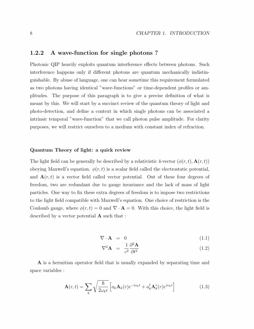
The light field can be generally be described by a relativistic 4-vector (φ(r, t),A(r, t))
obeying Maxwell’s equation. φ(r, t) is a scalar field called the electrostatic potential,
and A(r, t) is a vector field called vector potential. Out of these four degrees of
freedom, two are redundant due to gauge invariance and the lack of mass of light
particles. One way to fix these extra degrees of freedom is to impose two restrictions
to the light field compatible with Maxwell’s equation. One choice of restriction is the
Coulomb gauge, where φ(r, t) = 0 and ∇ ·A = 0. With this choice, the light field is
described by a vector potential A such that :
∇ ·A = 0 (1.1)
∇2A =1
c2
∂2A
∂t2(1.2)
A is a hermitian operator field that is usually expanded by separating time and
space variables :
A(r, t) =∑k
√~
2ωkε
[akAk(r)e
−iωkt + a†kA∗k(r)e
iωkt]
(1.3)

1.2. PHOTONIC APPROACH TO QUANTUM INFORMATION 9
Here k is an index labelling the different eigenmodes of Eq. (1.2), ωk the cor-
responding eigenfrequencies and Ak(r) the corresponding orthonormal spatial eigen-
functions. The dimensionless operators a†k and ak create and destroy respectively
a quantum of light in mode k. They obey the canonical commutation relation for
bosons[ak, a
†k′
]= δkk′ .
The relevant quantum mechanical operator describing the photo-detection prop-
erties of light [?] is the electric field operator:
E = −∂A∂t
= i∑k
√~ωk2ε
[akAk(r)e
−iωkt − a†kA∗k(r)e
iωkt]
(1.4)
This is indeed the observable that most photo-detectors respond to. The elec-
tric field is traditionally separated into its destruction and creation part : E(r, t) =
E(+)(r, t) + E(−)(r, t). With this notation, the probability amplitude of triggering a
photo-detector located in r at time t is proportional to: 〈f |E(+)(r, t) |i〉 where |i〉 and
|f〉 are the initial and final state of the light field.
For a single photon state |Ψ〉, the final state is always the vacuum, and the photo-
detection probability amplitude is proportional to: 〈vac|E(+)(r, t) |Ψ〉.
More precisely, if the initial photon state is:
|Ψ〉 =∑k
ckAk(r)a†k |vac〉
the transition probability amplitude at time t T (t) of a detector with spatial
response function D(r) is:
T (t) =∑k
√~ωk2ε
ck
[∫d3rD∗(r)Ak(r)
]e−iωkt (1.5)
D(r) describes in a sense the spatial sensitivity of the detector. For a single atom
making a transition between electronic levels |g〉 and |e〉, D(r) = erΨ∗e(r)Ψg(r) for
instance.

10 CHAPTER 1. INTRODUCTION
Given expression (1.5), it is natural to define the temporal ”wave-function” α(t) for
the photon with respect to a detector. We will use the term photon pulse amplitude
rather than wave-function since that term seems to be reserved to the solution of
a Schrodinger equation - which light does not satisfy (rather is satisfies Maxwell’s
equation which are differential of second order in time) :
α(t) = N∑k
√ωkck
[∫d3rD∗(r)Ak(r)
]e−iωkt (1.6)
For a given transverse mode of propagating light, with given dispersion ω(k), k
labels a continuum of longitudinal modes. Then denoting D(ω) = dkdω
the density of
longitudinal modes at frequency ω, we can write the photon pulse amplitude on the
detector as :
α(t) = N∫dωD(ω)
√ωc(ω)
[∫d3rD∗(r)Ak(ω)(r)
]e−iωt (1.7)
when the single photon state itself is defined by :
|Ψ〉 =
∫dωD(ω)c(ω)Ak(ω)(r)a
†(ω) |vac〉 (1.8)
So in general, the photo-detection amplitude is a joint property of the detector and
the single photon pulse. In the particular case where the function c(ω) has support on
a range of frequencies that is small compared to its central frequency, and where both
the mode density D(ω) and spatial overlap with the detector[∫d3rD∗(r)Ak(ω)(r)
]can be considered flat, the photo-detection amplitude reflects the intrinsic ”shape”
of the photon pulse. This condition is fulfilled in most experimental cases except
maybe in photonic band-gap wave-guides operating near the band-edge. Under this
restriction, the photon state seen by any such ”broadband” detector can be simplified
to :
|Ψ〉 =
∫dωc(ω)a†(ω) |vac〉 (1.9)
where we took away the space-dependent part on the ground that it gives constant
1.2. PHOTONIC APPROACH TO QUANTUM INFORMATION 11
overlap with the detector’s spatial response function. The photo-detection amplitude
becomes :
α(t) = N ′∫dωc(ω)e−iωt (1.10)
If we define the time-dependent annihilation operator as :
a(t) ≡ 1√2π
∫dωe−iωta(ω) (1.11)
we can finally write :
|Ψ〉 =
∫dtα(t)a†(t) |vac〉 (1.12)
where α(t), that we call the photon pulse amplitude, is proportional to the photo-
detection amplitude of a broadband detector. Throughout the text, we will assume
that∫|α(t)|2dt = 1 corresponding to an ideal detector perfectly matched spatially to
the transverse photonic mode. We can add empiric losses by hand if required as a
single factor called the quantum efficiency of the detector.
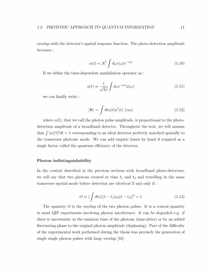
Photon indistinguishability
In the context described in the previous sections with broadband photo-detectors,
we will say that two photons created at time t1 and t2 and travelling in the same
transverse spatial mode before detection are identical if and only if :
O ≡ |∫dtα∗1(t− t1)α2(t− t2)|2 = 1 (1.13)
The quantity O is the overlap of the two photon pulses. It is a central quantity
in most QIP experiments involving photon interference. It can be degraded e.g. if
there is uncertainty in the emission time of the photons (time-jitter) or by an added
fluctuating phase to the original photon amplitude (dephasing). Part of the difficulty
of the experimental work performed during the thesis was precisely the generation of
single single photon pulses with large overlap [16].

12 CHAPTER 1. INTRODUCTION
1.3 Summary of thesis
The thesis work focuses generally on the development of single photon sources for
applications in quantum information. It contains two main parts. The first part
(chapters 2-4) is experimental and describes our efforts to develop QD-based single
photon sources, incoherently excited yet of high quality, and apply them in useful
QIP protocols. In chapter 2, we describe the principle of operation and fabrication
methods of such sources. We illustrate the usefulness of these sources by performing
two basic but fundamental QIP experiment: the formation of entanglement between
independent single photons (chapter 3) and a quantum teleportation protocol (chap-
ter 4). The second part of the thesis (chapter 5) exposes a general theory of coherent
single photon trapping and generation in a cavity QED system. It is proposed as a
necessary improvement of existing single photon sources for scalable quantum com-
puting applications. We indeed suggest an explicit model of quantum processor using
this technique with quantum dots in photonic crystal cavities and wave-guides.
Chapter 2
Single Photon source: Operation
principle
The single photon sources (SPS) used in the experiments throughout the thesis were
based on the fluorescence of a single semiconductor quantum dot (QD) [7] placed in
an optical micro-cavity. The same type of quantum dot was used (InAs/GaAs) but
the type of cavities varied from micropillars to photonic crystal slabs with different
geometries. In this chapter, we will first explain briefly the physics of QD and mi-
crocavities, and then how to combine both elements into a useful SPS usable is QIP
experiments. We describe the main characteristics of SPS and how to measure them.
2.1 Quantum Dots
In this section, we review the physics of a QD relevant to the operation of a SPS, and
give the experimental details of their fabrication.
2.1.1 Basic notions
A semiconductor QD is a cluster of semiconductor material embedded in a matrix
of another semiconductor of larger bandgap. The cluster is able to sustain trapped
(bound) states for both electrons in the conduction band and holes in the valence
13

14 CHAPTER 2. SINGLE PHOTON SOURCE: OPERATION PRINCIPLE
band (Fig. 2.1). Electrons and/or holes can indeed be trapped in QDs at cryogenic
temperatures. Although a QD is made of thousands of atoms, it has an effective
quantum mechanical description very similar to the one of a single atom if we define
effective masses for electrons and holes near the semiconductor band edges, account-
ing for their more complicated interaction with the crystal lattice. For that reason,
QD are often called ”artificial atoms”.
An electron-hole pair trapped in the QD is called a QD exciton. Excitons can
change state inside the QD, or recombine either radiatively or non-radiatevely. When
the electron is trapped in the ground state of the QD conduction band and the hole
is trapped in the ground state of the QD valence band, the main mode of decay for
the exciton is radiative recombination.
Electron discrete levelsConduction band
Hole discrete levels
n=1n=2
Valence band
n=2
n=1
InAsGaAs GaAs
Figure 2.1: Spatial variation of conduction and valence band energies in a QD.
2.1. QUANTUM DOTS 15
2.1.2 Fabrication method
The QD used in all the thesis worked are self-grown clusters of InAs on a susbtrate
of GaAs. The growth was performed by Molecular Beam Epitaxy (MBE), in the
Stranski-Krastanov method [17]. Since the InAs crystal has a 7% lattice mismatch
with GaAs, layers of InAs grown on top of a GaAs substrate experience mechanical
strain, which favorizes the formation of pyramidal clusters, typically a few nanometer
thick and 20-40 nm large.
Growth conditions have a strong effect on the optical properties of QDs. They
determine the amount of GaAs mixed in the InAs cluster, their sizes and shapes,
which all can change the spectrum of fluorescence from the QD. Growth conditions
also determine the density of recombination centers for electron-hole pairs at the
InAs/GaAs interface, which are mostly responsible for non-radiative decay of excitons.
2.1.3 Optical excitation methods
Excitons are formed in the QD either by capture of a free electron and a free hole
from the GaAs matrix, or by direct optical excitation of the InAs cluster. In the first
case, free carriers in the GaAs matrix can be created by a variety of means, including
electrical [18] or optical [19, 20, 21, 22].
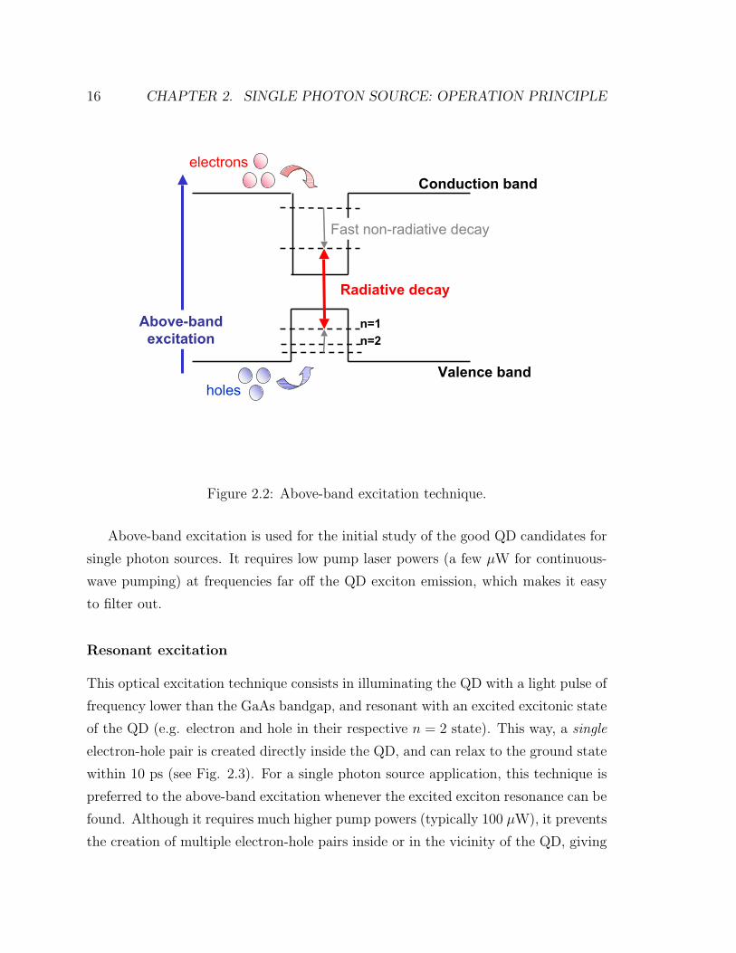
Above-band excitation
In this excitation technique, one illuminates the vicinity of the QD with a light pulse
of frequency greater than the GaAs bandgap. In such condition, many free electrons
and holes are generated in the GaAs matrix, and can diffuse to the QD. Electrons
and holes can be separately captured in the QD after some time, typically 100 ps.
Once inside the QD, they relax quickly to their ground state on a time scale of 10
ps (see Fig. 2.2). The relaxation mechanism is attributed to LO phonon scattering
[23, 24]. With this excitation technique, several excitons can be injected in the QD,
and give it a complex photoluminescence (PL) spectrum (Fig. 2.4).
16 CHAPTER 2. SINGLE PHOTON SOURCE: OPERATION PRINCIPLE
n=2n=1Above-band
excitation
Conduction band
Valence band
Radiative decay
Fast non-radiative decay
holes
electrons
Figure 2.2: Above-band excitation technique.
Above-band excitation is used for the initial study of the good QD candidates for
single photon sources. It requires low pump laser powers (a few µW for continuous-
wave pumping) at frequencies far off the QD exciton emission, which makes it easy
to filter out.
Resonant excitation
This optical excitation technique consists in illuminating the QD with a light pulse of
frequency lower than the GaAs bandgap, and resonant with an excited excitonic state
of the QD (e.g. electron and hole in their respective n = 2 state). This way, a single
electron-hole pair is created directly inside the QD, and can relax to the ground state
within 10 ps (see Fig. 2.3). For a single photon source application, this technique is
preferred to the above-band excitation whenever the excited exciton resonance can be
found. Although it requires much higher pump powers (typically 100 µW), it prevents
the creation of multiple electron-hole pairs inside or in the vicinity of the QD, giving

2.2. OPTICAL MICRO-CAVITIES 17
cleaner spectrum and avoiding re-pumping. It also greatly reduces the uncertainty in
the single photon emission time counted from the time we applied the exciting laser
pulse.
Conduction band
n=2n=1
Valence band
Radiative decay = 1 photon
Fast non-radiative decay
Resonantexcitation
Figure 2.3: Resonant excitation of a QD.
2.2 Optical micro-cavities
Placing a QD in a micro-cavity has two effects: it changes the light emission pattern,
and affects the exciton radiative decay rate. This last effect, known as the Purcell ef-
fect [25], is due to a modification of the structure of the electromagnetic field vacuum
around the QD. The strength of the Purcell effect is measured in terms of the ratio of
spontaneous emission of a QD exciton in a cavity and in bulk GaAs. It depends on
the spectral and spatial matching of the QD with respect to the cavity mode, and can
be greater or smaller than 1, corresponding to spontaneous emission enhancement or
suppression by the cavity.
A micro-cavity can greatly enhance the performance of a SPS. By redirecting the
light emission, it can help improving the light collection efficiency which is the major

18 CHAPTER 2. SINGLE PHOTON SOURCE: OPERATION PRINCIPLE
Inte
nsity
Above-Band Excitation
Wavelength (nm)In
tens
ity
Resonant excitation
Wavelength (nm)
Figure 2.4: Photoluminescence spectra of a single QD under above-band or resonantexcitation.
source of photon loss in current systems. Also, it can reduce the photon temporal
width, lowering the impact of potential exciton state dephasing on the quantum in-
distinguishability of photons. Another practical effect of small cavities is to isolate a
few quantum dots so they can be dealt with individually.
The SPS used in the thesis work used two types of micro-cavities, first micropillars
and later on 2D photonic crystal structures.
2.2.1 Micropillar cavities
Micropillar cavities were analyzed theoretically in details in [26, 27]. They confine
light in the vertical direction by distributed Bragg reflection (DBR), and in the par-
tially in the lateral direction by total internal reflection. They have a radiation
pattern shaped as a single-lobed Gaussian which facilitates the coupling to single
mode fibers. It is also relatively straightforward to isolate a single QD in them. The
structures used for the thesis work were constructed by a combination of molecular
beam epitaxy (MBE) and chemically assisted ion beam etching (CAIBE). MBE is
used to grow a wafer consisting of self-assembled InAs QDs embedded in the middle

2.2. OPTICAL MICRO-CAVITIES 19
of a GaAs spacer layer, and sandwiched between DBR mirrors. The GaAs spacer
is approximately one optical wavelength thick (274 nm), and DBR mirrors are con-
structed by stacking quarter-wavelength thick GaAs and AlAs layers on top of each
other. The grown wafer has twelve DBR pairs above, and thirty DBR pairs below
the spacer. Microposts with diameters ranging from 0.3 µm to 5 µm and heights of
4.8 µm are fabricated ar random spatial locations by CAIBE, with Ar+ ions and Cl2
gas, and using sapphire dust particles as etch masks. Due to the irregular shapes of
the posts, the fundamental HE11 mode is typically polarization-nondegenerate. Many
microposts have only one or two QDs on resonance with the fundamental cavity mode.
ECR CAIBE
Figure 2.5: Micropillar cavities used in the QIP experiments of this work. The bestcavities, shown on the right, were etched by chemically assisted ion beam etching(CAIBE) with a mask of sapphire dust.
2.2.2 Photonic bandgap cavities
Photonic bandgap (PBG) cavities are in a sense dual structures to micropillars. They
consist in a two-dimensional photonic crystal slab with a punctual defect, in which
light is confined horizontally by DBR effect and vertically by total internal reflection.
Design
The design of PBG cavities constitute a research object in itself, realized mostly by
computer simulation. Maxwell’s equations are solved for various proposed design with
20 CHAPTER 2. SINGLE PHOTON SOURCE: OPERATION PRINCIPLE
a numerical technique called Finite difference time domain (FDTD). The fine tuning
of hole size and position around the defect determines the resonance wavelength, the
mode volume and the quality factor of the cavity. A common difficulty in obtaining
large quality factors is the fact that increased confinement in the lateral direction
increases the amount of losses in the vertical direction (diffraction), so a balance has
to be found.
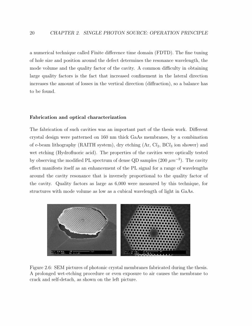
Fabrication and optical characterization
The fabrication of such cavities was an important part of the thesis work. Different
crystal design were patterned on 160 nm thick GaAs membranes, by a combination
of e-beam lithography (RAITH system), dry etching (Ar, Cl2, BCl3 ion shower) and
wet etching (Hydrofluoric acid). The properties of the cavities were optically tested
by observing the modified PL spectrum of dense QD samples (200 µm−2). The cavity
effect manifests itself as an enhancement of the PL signal for a range of wavelengths
around the cavity resonance that is inversely proportional to the quality factor of
the cavity. Quality factors as large as 6,000 were measured by this technique, for
structures with mode volume as low as a cubical wavelength of light in GaAs.
Figure 2.6: SEM pictures of photonic crystal membranes fabricated during the thesis.A prolonged wet-etching procedure or even exposure to air causes the membrane tocrack and self-detach, as shown on the left picture.
2.2. OPTICAL MICRO-CAVITIES 21
Spontaneous emission suppression and enhancement by PBG cavities
The effect on the cavity on a single QD spontaneous emission properties varies a lot
depending on the spatial, spectral and polarization matching of the exciton dipole to
the electric field of the cavity mode. Suppose a single QD with exciton dipole moment−→µ and transition wavelength λ is located at position r in a cavity mode of quality
factor Q, resonance wavelength λc, and electric field pattern E(r). The cavity mode
volume is defined as :
Vm =
∫d3r ε(r)|E(r)|2
Maxr [ε(r)|E(r)|2](2.1)
The spontaneous emission rate Γ of the exciton compared to the rate in bulk GaAs
Γ0 is then predicted to be :
Γ
Γ0
= Fp
( −→E (r) · −→µ|−→Emax||−→µ |
)21
1 + 4Q2(λλc− 1)2 + FPC (2.2)
Here Fp = 34π2
λ3
n3QVm
is the maximum relative emission rate directly in the cavity
mode (Purcell factor), and FPC is the relative emission rate in the rest of the pho-
tonic crystal, in the so-called ”leaky modes”. Notice the lorentzian dependence of
the cavity emission rate on the exciton wavelength. When the exciton wavelength
is near cavity resonance, its radiative decay rate can become well above its value in
bulk GaAs. We indeed measured enhancement factors as large as 10 using a streak
camera system [?]. On the other hand, if the exciton wavelength is far off-resonance,
it can in principle show suppressed spontaneous emission. We observed that effect as
well for the first time in photonic crystal cavities. Important spontaneous emission
quenching factors as large as 5 could be measured.
When the QD-cavity coupling become greater than the cavity decay rate, the QD
does not simply decay but is in theory able to exchange energy coherently with the
cavity, a phenomenon known as Rabi oscillations. This is the so-called regime of
”strong coupling”. The effect of the cavity on the QD in the strong coupling regime

22 CHAPTER 2. SINGLE PHOTON SOURCE: OPERATION PRINCIPLE
can not be summarized by a single rate enhancement factor. In appendix A, we derive
explicitly the spectrum of the light emitted from the QD through the cavity mode
and in the leaky modes. During the thesis, we observed no conclusive evidence for
strong coupling. This effect is still being sought for actively in our labs.
2.3 Single photon generation
The principle of single photon generation is explained in details in [28]. A single
quantum dot placed in an optical cavity is excited either resonantly or above-band
with a short Ti:Sa laser pulse (200 fs - 2 ps). The temperature is adjusted to improve
the spectral matching of the exciton transition to the cavity resonance if needed. The
fluorescent photon emitted by a single QD exciton is collected with a microscope
objective and collimated for further applications (e.g. in free space or optical fibers).
Additional narrow spectral filtering is applied around the single exciton wavelength,
to eliminate spurious multi-exciton or charged exciton emission. The figures of merit
of single photon sources are three-fold: quantum efficiency, degree of anti-bunching,
quantum indistinguishability. In this section, we summarize the temperature tuning
technique, and go on to explain how to measure the source parameters.
2.3.1 Temperature tuning
By tuning the sample temperature in the range between 6 K and 40 K, the QD
emission wavelength can be tuned throughout a cavity resonance, as illustrated in
Figure 2.8. In this figure, the emission rate of a QD is plotted as a function of the
detuning between the QD emission and the cavity resonance. The cavity resonance
(see the top right inset of the figure) is red-shifted by roughly 0.3 nm by increasing
temperature in the studied range. This shift is included in plotting the data. A
good matching is observed between our experiment and the theoretically predicted
Lorentzian behavior [29]
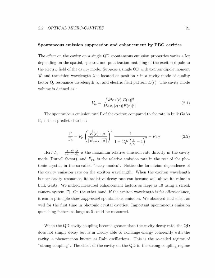
2.3. SINGLE PHOTON GENERATION 23
spectro-meter
streak camerasystem
CCD
Photon correlation(HBT-type) setup
Time-resolved spectra
Photon counterscryostatpinholefilter
NPBS
Ti-Sapphire laser(2 ps pulses every 13 ns)
Figure 2.7: Single photon source characterization setup used with micropillar samples.With PBG samples, a confocal microscope setup was preferred to the side excitationshown here , so that a narrow region (submicron) only could be illuminated.
2.3.2 Quantum efficiency
The quantum efficiency is simply the probability that a photon is collected from
the QD after photo-excitation. It can be measured knowing the repetition rate of the
exciting pulses, and the photo-detection rate of the light signal from the QD measured
by a photo-avalanche device of known efficiency (here Perkin-Elmers single photon
counter modules or ”SPCM”, 40% efficient at QD wavelength). The highest quantum
efficiency measured on a SPS device during the thesis work was 2% for a micropillar
structure, most of the loss occurring in the light collection process.

24 CHAPTER 2. SINGLE PHOTON SOURCE: OPERATION PRINCIPLE
Figure 2.8: Measured spontaneous emission rate of a QD exciton in a micropillarcavity, as a function of its detuning from the cavity resonance. The dot emissionwavelength is tuned by changing the sample temperature within the 6 K - 40 Krange. The top left inset illustrates the lifetime modification of the same QD on-and off-resonance, the top right inset illustrates the cavity resonance, and the bottomright inset corresponds to an SEM micrograph of the micropillar structure.

2.3. SINGLE PHOTON GENERATION 25
2.3.3 Degree of anti-bunching
The degree of anti-bunching reflects the occurrence of multi-photon pulses from the
QD. It is measured by the equal-time intensity auto-correlation factor g(2)(0), which
is related to the photon number (n) statistics according to :
g(2)(0) =〈n(n− 1)〉〈n〉2
(2.3)
For a classical light pulse of arbitrary intensity g(2)(0) ≥ 1 and g(2)(0) = 1 for
coherent states (laser pulses). For a true single photon source (even a lossy one),
g(2)(0) = 0.
In practice, the intensity auto-correlation factor g(2)(τ) can be measured in a
Hanbury-Brown-Twiss (HBT) type setup as shown in Fig. 2.7. We split the light
signal form a light source is split in a beam-splitter (BS), and record the number of
coincidental photo-detection events at different ports of the BS happening with time
difference τ . This gives a correlation histogram of coincidence counts versus time
difference, as shown in Fig. 2.9. The number of coincidence counts recorded for time
difference τ is proportional to the conditional probability of presence of a photon at
time t = τ given the presence of a photon at time t = 0.
Our single photon sources usually had better g(2)(0) factors when excited reso-
nantly rather than above band. This might be due to the fact that in the above-band
case, a single QD can re-absorb an electron-hole pair from the surrounding GaAs after
emission of a photon. Measured g(2)(0) values were routinely in the range 20-50% for
above-band excitation, and 5-20% for resonant excitation. The best measured value
was 2% for a resonantly excited micropillar SPS.
2.3.4 Quantum indistinguishability
As we said earlier, the quantum indistinguishability of photons emitted by the source
is of central importance for many QIP applications. It can be measured as the overlap

26 CHAPTER 2. SINGLE PHOTON SOURCE: OPERATION PRINCIPLEC
oinc
iden
ce c
ount
s
Delay τ (ns)
Figure 2.9: Intensity auto-correlation histogram. g(2)(0) is given by the ratio ofcoincidence counts in the ”central” peak and in a ”side” peak.
between photon pulse amplitudes, as defined in the last chapter.
Experimentally we can measure the average overlap between consecutive photon
pulses emitted by a SPS by observing the so-called photon bunching effect. Due to
their bosonic nature, two identical photons ”colliding” in a 50-50% beam-splitter are
expected to always take the same exit path. Hence if photo-detectors are placed
on each exit, they should never record a coincidence count. This is strictly true
however only if the two photon pulses are identical. If the photon overlap is reduced
to values smaller than 1, the detectors record coincidence counts in proportion. This
can be understood from the formalism developed in the last chapter. Denote a, b
(c, d) the input (output) modes of the BS. The input/output operators are related by
the unitary BS matrix :
a =c+ d√
2(2.4)
b =c− d√
2(2.5)
If α(t) and β(t) are the photon pulse amplitudes as seen by broadband detectors,
the quantum mechanical state of the input light field is :

2.3. SINGLE PHOTON GENERATION 27
|Ψ〉 =∫ds α(s)a†(s)
∫du β(u)b†(u) |V ac〉
= 12
∫ ∫ds duα(s)β(u)[c†(s)c†(u)− d†(s)d†(u)] |V ac〉
+12
∫ ∫ds duα(s)β(u)[d†(s)c†(u)− c†(s)d†(u)] |V ac〉
(2.6)
In Eq. (2.6), the first term contributes to a bunched outcome (photons take same
path) while the second term contributes to an anti-bunched outcome (photons take
different path). The probability of triggering both detectors is :
Pcoinc =
∫dt
∫dτ 〈Ψ| c†(t)c(t) d†(t+ τ)d(t+ τ) |Ψ〉 (2.7)
=1
2
[1−
∣∣∣∣∫ dtα∗(t)β(t)
∣∣∣∣2]
(2.8)
and indeed vanishes for identical photon pulses.
Photon overlaps were routinely measured in a Mandel-type setup shown in Fig.
2.10. Two photons emitted from a SPS with 2 ns interval were made to collide on a
50-50% BS. One fourth of the time, they would indeed enter the BS simultaneously,
and the rest of the time they would miss each other, which makes the pattern of
coincidence counts on the correlation histogram somewhat complicated (Fig. 2.11).
The degradation of overlap of two consecutive photons is directly proportional to the
number of equal-time coincidence counts on the histogram, and by comparison with
side peaks, the average overlap between consecutive photons can be extracted. The
best overlap value (81%) was measured on a micropillar structure. Overlap values
in the 50-70% range were routinely observed on other micropillar structures under
resonant excitation.
We attribute the degradation of overlap to two phenomenon: exciton dephasing
and emission-time jitter. If the energy of the exciton state fluctuates with dephas-
ing time τd, a random phase is imprinted on the single photons produced, and their
overlap drops by a factor of τdτd+2τex
where τex is the exciton decay time. If there is

28 CHAPTER 2. SINGLE PHOTON SOURCE: OPERATION PRINCIPLE
Photodetectors τ
2 ns delay2 ns
Lens (collimation)Retro-reflector cubes
Figure 2.10: Mandel-type setup used to perform a photon bunching experiment andmeasure the overlap of photons emitted consecutively in a SPS. Pairs of consecutivephotons separated by 2 ns are generated every 13 ns by resonant excitation.
Coi
ncid
ence
cou
nts Dip
Detection time difference τ [ns]
Figure 2.11: Correlation histogram resulting from a photon bunching experiment.The overlap of consecutive photons can be inferred from the depth of the central dip.
2.3. SINGLE PHOTON GENERATION 29
some uncertainty ∆τ in the emission time, the two photons will partially miss each
other at the BS, resulting in a degradation of overlap by a factor of τexτex+∆τ
. To be
indistinguishable, photons have to be produced on a time scale long compared to the
jitter time ∆τ but short compared to the dephasing time τd. With InAs/GaAs QDs,
we estimated ∆τ ∼ 10 ps and τd ∼ 2 ns. The natural exciton decay time in these
QDs are usually between 500 ps and 1.5 ns, but was reduced to values as low as 100
ps with the use of optical cavities, which is close to optimal.
Dephasing and time-jitter set an intrinsic limit to achievable photon indistin-
guishability using the described photon production method. The best overlap that
could be achieve is somewhere around 90%, which is enough to realize QIP protocols
with a small number of qubits, but not nearly high enough to factorize large numbers.
In chapter 5, we will propose a new way of producing photons that circumvent the
emission-time uncertainty problem and will allow the design of fast SPS with higher
photon overlaps.
Chapter 3
Entanglement formation
This chapter describes an optical QIP experiment in which polarization-entangled
photons were created using a quantum dot single photon source, linear optics and
photodetectors. Two photons created independently at different times in the pho-
ton source show polarization correlations that violate Bell’s inequality. The density
matrix describing the polarization state of the post-selected photon pairs is recon-
structed, and agrees well with a simple model predicting the quality of entanglement
from the known parameters of the single photon source: intensity auto-correlation
factor g(2)(0) and photon overlap O. Our scheme provides a method to create a sin-
gle entangled photon pair per cycle after post-selection, a feature useful to enhance
quantum cryptography protocols based on shared entanglement.
3.1 Description of experiment
3.1.1 Background
Entanglement, the non-local correlations allowed by quantum mechanics between dis-
tinct systems, is a central concept of quantum information science [30]. Traditionally,
these non-local correlations were often understood as the result of prior interactions
between the quantum mechanical systems, something like a memory of those inter-
actions. In the light of recent progress in the field of quantum information (see e.g.
30

3.1. DESCRIPTION OF EXPERIMENT 31
the Innsbruck teleportation experiment [31]), this is too limited a view. Entangle-
ment can be induced between non-interacting particles, provided they are quantum
mechanically indistinguishable. In this type of scheme, an auxiliary degree of free-
dom such as the particle number is measured, and the result of that measurement is
feed-forwarded to the next step of processing. For instance, the experimental data
can be postselected based on the ”click” of particle detectors. Pionneering work by
Shih and Alley [32], followed by Ou and Mandel [33], already used this post-selection
procedure to induce entanglement between two identical photons produced in a non-
linear crystal. More recently, entanglement swapping experiments [34, 35] used two
independent entangled photon pairs to induce entanglement between photons of dif-
ferent pairs which never interacted. Here we use a similar linear optics technique to
induce polarization entanglement between single photons emitted independently in
a semiconductor quantum dot source, 2 ns apart. We observed a clear violation of
Bell’s inequality (BI), which constitutes an experimental proof of non-local behavior
for the first time with a semiconductor single photon source. The complete density
matrix describing the polarization state of the two photons was also reconstructed,
and satisfies the Peres criterion for entanglement [36]. We show that our results can
be quantitatively explained in terms of basic parameters of the single photon source
and derive a simple criterion for entanglement generation using those parameters.
Eventually, we explain why our technique can be applied to quantum key distribu-
tion (QKD) in a straightforward and useful manner.
3.1.2 Entanglement formation principle
This experiment relies on two crucial features of our quantum dot single photon
source, namely its ability to suppress multi-photon pulses [37], and its ability to gen-
erate consecutively two photons that are quantum mechanically indistinguishable [16].
The idea is to ”collide” these photons with orthogonal polarizations at two conjugated
input ports of a non-polarizing beam splitter (NPBS). A quantum interference effect
ensures that photons simultaneously detected at different output ports of the NPBS
should be entangled in polarization [33]. More precisely, when the two optical modes

32 CHAPTER 3. ENTANGLEMENT FORMATION
corresponding to the output ports ’c’ and ’d’ of the NPBS have a simultaneous single
occupation, their joint polarization state is expected to be the EPR-Bell state:
∣∣Ψ−⟩ =1√2
(|H〉c |V 〉d − |V 〉c |H〉d)
Denoting ’a’ and ’b’ the input port modes of the NPBS, they are related to the output
modes ’c’ and ’d’ by the 50-50% NPBS unitary matrix according to:
aH/V =1√2
(cH/V + dH/V )
bH/V =1√2
(cH/V − dH/V )
where subscripts ’H’ and ’V’ specify the polarization (horizontal or vertical) of a
given spatial mode. The quantum state corresponding to single-mode photons with
orthogonal polarizations at port ’a’ and ’b’ can be written as:
a†Hb†V |vac〉 =
1
2(c†Hc
†V − d
†Hd†V − c
†Hd†V + c†V d
†H) |vac〉
As pointed out in [38], this state already features non-local correlations and violates
Bell’s inequality without the need for post-selection, by using photo-detectors that can
distinguish photon numbers 0,1 and 2. However, since the quantum efficiency of our
source is too low (typically 0.1% to 2%) to implement such a ”loophole-free” BI test,
we implemented a simpler scheme using post-selection based on the simultaneous click
of two regular photon counter modules. If we discard the events when two photons
go the same way (recording only coincidence events between modes ’c’ and ’d’), we
obtain the post-selected state:
1√2
(c†Hd†V − c
†V d†H) |vac〉 =
∣∣Ψ−⟩with a probability of 1
2.
3.1. DESCRIPTION OF EXPERIMENT 33
3.1.3 Method
The experimental setup is shown in fig 3.1. The single photon source consists of a
self-assembled InAs quantum dot (QD) embedded in a GaAs/AlAs DBR microcavity
[16]. It was placed in a Helium flow cryostat and cooled down to 4-10 K. Single
photon emission was triggered by resonant optical excitation of a single QD, isolated
in a micropillar cavity. We used 3 ps Ti:Sa laser pulses on resonance with an excited
state of the QD, insuring fast creation of an electron-hole pair directly inside the QD.
Pulses came by pairs separated by 2 ns, with a repetition rate of 1 pair/13 ns. The
emitted photons were collected by a single mode fiber and sent to a Mach-Zehnder
type setup with 2 ns delay on the longer arm. A quarter wave plate (QWP) followed
by a half wave plate (HWP) were used to set the polarization of the photons after
the input fiber to linear and horizontal. An extra half wave plate was inserted in the
longer arm of the interferometer to rotate the polarization to vertical. One time out
of four, the first emitted photon takes the long path while the second photon takes
the short path, in which case their wavefunctions overlap at the second non-polarizing
beam-splitter (NPBS 2). In all other cases (not of interest), the single photon pulses
”miss” each other by at least 2 ns which is greater than their width (100 - 200 ps).
Two single photon counter modules (SPCMs) in a start-stop configuration were used
to record coincidence counts between the two output ports of NPBS 2, effectively
implementing the post-selection (if photons exit NPBS 2 by the same port, then no
coincidence are recorded by the detectors). Single-mode fibers were used prior to
detection to facilitate the spatial mode-matching requirements. They were preceded
by quarter wave and polarizer plates to allow the analysis of all possible polarizations.
The detectors were linked to a time-to-amplitude converter, which allowed to
record histograms of coincidence events versus detection time delay τ . A typical his-
togram is shown on fig 3.2, with the corresponding post-selected events. For given
analyzer settings (α, β), we denote by C(α, β) the number of post-selected events
normalized by the total number of coincidences in a time window of 100 ns. This
normalization is independent of (α, β) since the input of NPBS 2 are two modes with

34 CHAPTER 3. ENTANGLEMENT FORMATION
from QD
Single modefibers
2 nsH
pol,. control
2 nsAHWP
V
B
H HNPBS 2 NPBS 1
Figure 3.1: Experimental setup. Single photons from the QD microcavity device aresent through a single mode fiber, and have their polarization rotated to H. Theyare split by a first NPBS (1). The polarization is changed to V in the longer armof the Mach-Zehnder configuration. The two path of the interferometer merge at asecond NPBS (2). The output modes of NPBS 2 are matched to single mode fibersfor subsequent detection. The detectors are linked to a time-to-amplitude converterfor a record of coincidence counts.

3.1. DESCRIPTION OF EXPERIMENT 35
orthogonal polarizations. C(α, β) measures the average rate of coincidences through-
out the time of integration.
−13 −2 0 2 130
5
10
15
20
25
30
35
Time delay at NPBS 2 (ns)
Rec
ord
ed c
oin
cid
ence
s
Integration window
76
176
81
165
92
Peak area
Figure 3.2: Zoom on a typical correlation histogram, taken on QD1. Coincidenceswith delay τ between detectors A and B were actually recorded for −50ns < τ <50ns. The integration time was 2 min, short enough to guarantee that the QDis illuminated by a constant pump power. The central region −1ns < τ < 1nscorresponds to the post-selected events: the corresponding photons overlapped atNPBS 2 where they took different exit ports.
Two different QD microcavity devices were used to produce single photons. The
single count rate for QD 1 at the output of the single-mode fiber was 9400 counts/s,
from which we infer a total quantum efficiency of 0.13 % (detection loss included).
The total pair production rate for QD 1 was 12 /s after fiber, so that useful pairs were
generated with a rate of 1.5 /s (we loose a factor 8 due to the post-selection and by
excluding ”bad-timing” events). Both QD 1 and QD 2 featured a high suppression of
36 CHAPTER 3. ENTANGLEMENT FORMATION
two-photon pulses and high mean overlap (indistinguishability) between consecutive
photons. The overlap was measured in a photon bunching experiment [16], which
was realized by removing the HWP in the long arm, allowing photon pulses of same
polarization to collide in NPBS 2.
3.2 Results
Several methods can be used to prove the success of entanglement generation. The
traditional method is a Bell inequality test, that proves the non-local nature of the
state of two quantum systems if they are sufficiently entangled. Another more com-
plete way is to reconstruct the full density matrix describing the joint polarization
state of two photons, by a technique named quantum state tomography. The presence
of entanglement can then be read from the density matrix by several mathematical
methods.
3.2.1 Bell inequality test
A BI test was performed for post-selected photon pairs from QD1. Following ref [39],
if we define the correlation function E(α, β) for analyser settings α and β as:
E(α, β) =C(α, β) + C(α⊥, β⊥)− C(α⊥, β)− C(α, β⊥)
C(α, β) + C(α⊥, β⊥) + C(α⊥, β) + C(α, β⊥)
then local realistic assumptions lead to the inequality:
S = |E(α, β)− E(α′, β)|+ |E(α′, β′) + E(α, β′)| ≤ 2
that can be violated by quantum mechanics.
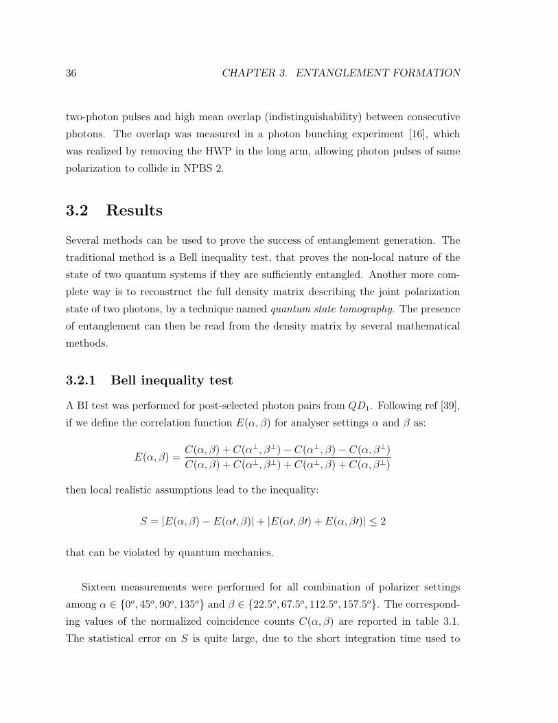
Sixteen measurements were performed for all combination of polarizer settings
among α ∈ 0o, 45o, 90o, 135o and β ∈ 22.5o, 67.5o, 112.5o, 157.5o. The correspond-
ing values of the normalized coincidence counts C(α, β) are reported in table 3.1.
The statistical error on S is quite large, due to the short integration time used to
3.2. RESULTS 37
β \α 0o 45o 90o 135o
22.5o 5.6 28.4 28.6 4.767.5o 9.0 8.3 25.2 25.1112.5o 28.9 5.4 4.6 28.4157.5o 26.0 24.9 8.6 8.8
Table 3.1: Normalized coincidence counts C(α, β) · 103 for various polarizer anglesused in the Bell Inequality test. They correspond to the coincidences in the integrationwindow (see fig. 3.2) divided by the total coincidences recorded for −50ns < τ <50ns. Note that the quantity C(α, β) +C(α⊥, β⊥) +C(α⊥, β) +C(α, β⊥) is constantfor given settings α and β.
insure high stability of the QD device. Bell’s inequality is still violated by two stan-
dard deviations, according to S ∼ 2.38 ± 0.18. Hence, non-local correlations were
created between two single independent photons by linear-optics and photon number
post-selection.
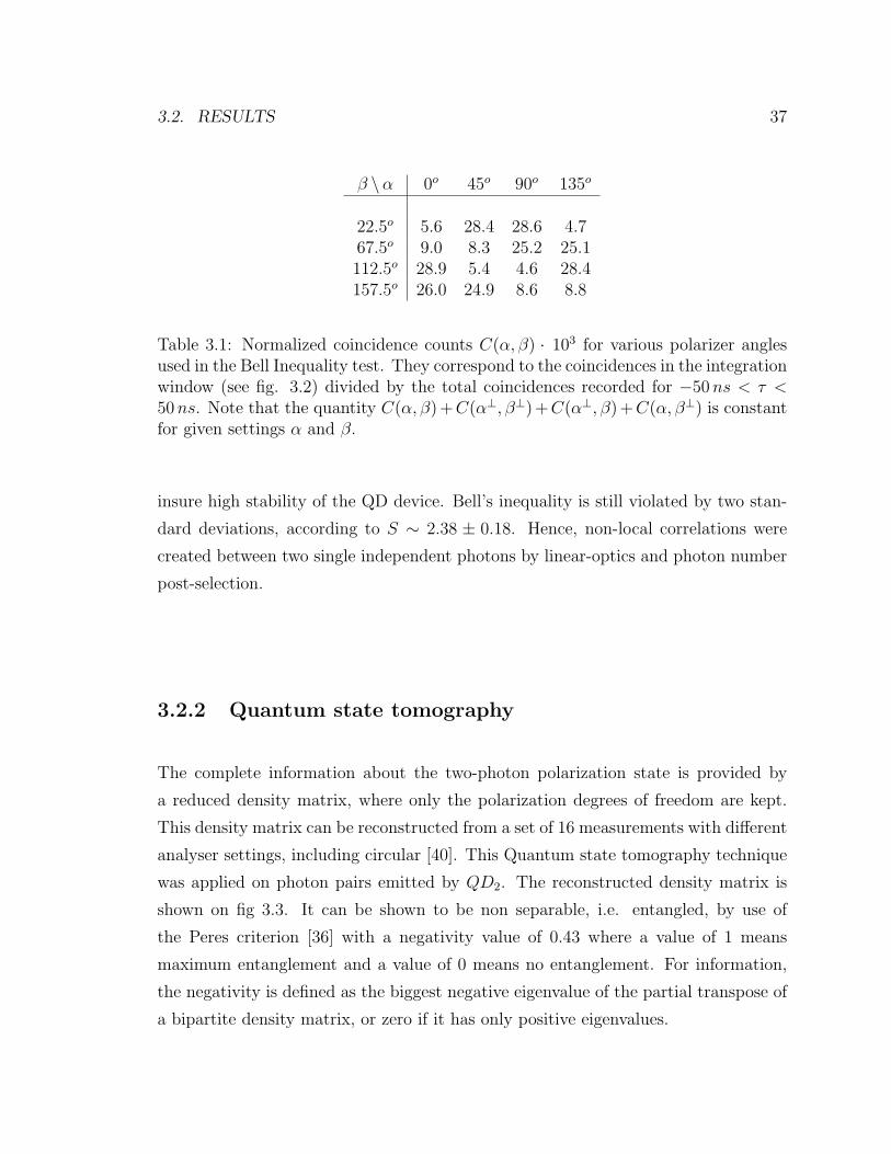
3.2.2 Quantum state tomography
The complete information about the two-photon polarization state is provided by
a reduced density matrix, where only the polarization degrees of freedom are kept.
This density matrix can be reconstructed from a set of 16 measurements with different
analyser settings, including circular [40]. This Quantum state tomography technique
was applied on photon pairs emitted by QD2. The reconstructed density matrix is
shown on fig 3.3. It can be shown to be non separable, i.e. entangled, by use of
the Peres criterion [36] with a negativity value of 0.43 where a value of 1 means
maximum entanglement and a value of 0 means no entanglement. For information,
the negativity is defined as the biggest negative eigenvalue of the partial transpose of
a bipartite density matrix, or zero if it has only positive eigenvalues.
38 CHAPTER 3. ENTANGLEMENT FORMATION
HHHV
VHVV
HH
HV
VH
VV
0
0.25
0.5
Real component
HHHV
VHVV
HH
HV
VH
VV
0
0.25
0.5
HHHV
VHVV
HH
HV
VH
VV
0
0.25
0.5
HHHV
VHVV
HH
HV
VH
VV
0
0.25
0.5
Real component
Imaginary component
Imaginary component
EXPERIMENT
IDEAL
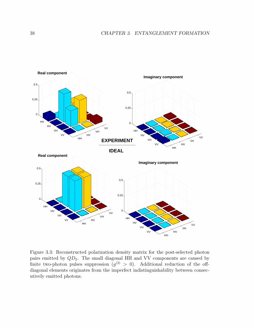
Figure 3.3: Reconstructed polarization density matrix for the post-selected photonpairs emitted by QD2. The small diagonal HH and VV components are caused byfinite two-photon pulses suppression (g(2) > 0). Additional reduction of the off-diagonal elements originates from the imperfect indistinguishability between consec-utively emitted photons.
3.2. RESULTS 39
3.2.3 Discussion
Model for density matrix
We try to account for the observed degree of entanglement solely by considering
some parameters of the QD single photon source. Due to residual two-photon pulses
(reflected by a non-zero value of the intensity auto-correlation factor g(2)(0) [37]), a
recorded coincidence count can originate from two photons of same polarization that
would have entered NPBS 2 from the same port. A multi-mode analysis also reveals
that an imperfect overlap O =∣∣∫ ψ1(t)∗ψ2(t)
∣∣2 between consecutive photon pulse
amplitudes washes out the quantum interference responsible for the entanglement
generation. Including those imperfections, we could derive a simple model for the
joint polarization state of the post-selected photons. In the limit of low pump level,
this model predicts the following density matrix in the (H/V)⊗(H/V) basis:
ρmodel =1
RT
+ TR
+ 4g(2)
2g(2)
RT−V
−V TR
2g(2)
R and T are the reflection and transmission coefficients of NPBS 2 (R
T∼ 1.1 in our
case). Using the values for g(2) and O measured independently, we obtain an excel-
lent quantitative agreement of our model to the experimental data, with a fidelity
Tr
(√ρ
12exp ρmodel ρ
12exp
)as high as 0.997.
The negativity of the state ρmodel is proportional to (V − 2g(2)), which means that
entanglement exists as long as V > 2g(2). This simple criterion can be applied to
any single photon source for which the intensity auto-correlation and photon overlap
values are known. It indicates to what extent that source will be able to generate
entangled photons with this beam-splitter scheme.

40 CHAPTER 3. ENTANGLEMENT FORMATION
Loop-hole free Bell inequality test ?
The experimental setup described here does not permit the distinction between pho-
ton numbers 0,1,2, and for that reason half of the photon pairs colliding at NPBS 2
only can be used for a BI test. However, following [38], it would be possible to design
a loophole-free BI test by keeping track of photon numbers with existing single pho-
ton resolution detectors [41], if however the quantum efficiency of the single photon
source could be made close to unity.
Application to quantum cryptography ?
Due to the need for post-selection, the current scheme does not allow the creation of an
”event-ready” entangled photon pair. This is a serious obstacle for many applications
to quantum information systems, but not all. The Ekert91 [42] or BBM92 [43] QKD
protocols using entangled photons can directly be performed with our post-selected
technique. The essence of these protocols is to establish a secure key upon local
measurement of two distant photons from an entangled pair, which is exactly similar
to our scheme. The bit error induced by uncorrelated photon pairs in those protocols is
significantly suppressed [44] when single entangled pairs are used, a feature which only
our source possesses among the currently demonstrated entangled photon sources.
Therefore, those QKD protocols should actually benefit from our method to generate
entanglement.
Making the scheme deterministic with QND detectors
The need for post-selection could be bypassed if we could use quantum non-demolition
(QND) photon number detectors, able to discriminate odd from even photon num-
bers. Suppose we have such a detector. If an even number of photon (either 0 or 2)
is detected in the same output mode ’c’ or ’d’ of NPBS 2, then we re-orient these
modes so that they mix in an auxiliary NPBS, to obtain with certainty the entangled
state |ψ+〉 in the exit. That state can be converted to |ψ−〉 with a half-wave plate.
If an odd number of photon (actually one) is detected in a given mode, then we do
nothing and obtain |ψ−〉 like in the original post-selected scheme.
3.2. RESULTS 41
Conclusion
In summary, we demonstrated the violation of Bell’s inequality for the first time with a
semiconductor single photon source. Polarization entanglement was induced between
two independent but indistinguishable single photons, with linear-optics and post-
selection based on the click of regular photon counters. Our cycle, which is a unique
feature among previously demonstrated entangled photon sources. Our scheme can
be straightforwardly applied to Ekert91/ BBM92 QKD protocols, and provided the
efficiency of the single photon source can be increased, would perform better than
current entangled photon sources for that purpose.

Chapter 4
Single Mode Teleportation
This chapter describes the experimental demonstration of a quantum teleportation
protocol with a micropillar single photon source. Two dual-rail optical qubits, a tar-
get and an ancilla each defined as a single photon delocalized between two different
free-space paths, were generated independently by the single photon source. By a
destructive measurement made on two path, one for each qubit, and postselection,
the state of the qubit encoded in the two remaining paths was found to reproduce
the state of the target qubit. In particular, the coherence between the different op-
tical path making the target qubit was transferred to the output paths to a large
extent. The observed fidelity is 80 %, in agreement with the residual distinguisha-
bility between consecutive photons from the source. An improved version of this
teleportation scheme using more ancillas is the building block of several proposals of
quantum computing with linear-optics and photo-detectors.
4.1 Description of experiment
4.1.1 Background
We already mentioned that photons are almost ideal carriers of quantum information,
since they have little interaction with their environment, and are easy to manipulate
individually with linear-optics. The main challenge of optical quantum information
42
4.1. DESCRIPTION OF EXPERIMENT 43
processing is the design of controlled interactions between photons, necessary for the
realization of non-linear quantum gates. Photons do not naturally ”feel” the presence
of other photons, unless they propagate in a medium with high optical non-linearity.
The amount of optical non-linearity required to perform controlled operations between
single photons is however not easily accessible. Large optical non-linearities having
noticeable effect at the single photon level might become eventually available with
the development of cavity QED or electromagnetically-induced transparency (EIT)
techniques, but these possibilities remain quite remote in the future.
Probabilistic gates can be implemented with linear-optics only [45, 46, 47], but
as such, they are not suitable for scalable quantum computation. In a seminal pa-
per [48], Gottesman and Chuang suggested that quantum gates could be applied to
photonic qubits through a generalization of quantum teleportation [49]. In such a
scheme, the information about the gate is contained in the state of ancilla qubits.
The implementation of a certain class of gates can then be reduced to the problem
of preparing the ancilla qubits in some wisely chosen entangled state. Such a prob-
lem can be solved ”off-line” with linear-optics elements only, provided the photons
used are quantum mechanically indistinguishable particles [31]. Following this idea,
Knill, Laflamme and Milburn (KLM) [46] proposed a scheme for efficient linear-optics
quantum computation (LOQC) based on the implementation of the controlled-sign
gate (C-z gate) through teleportation. Since the C-z gate acts effectively on only one
of the two modes composing the target qubit, a simplified procedure can be used
where a single optical mode is teleported, instead of the two modes composing the
qubit. This procedure will be referred to as single mode teleportation to distinguish
it from the usual teleportation scheme. In its basic version using one ancilla qubit, it
succeeds half of the time. In its improved version using an arbitrarily high number
of ancillas, it can succeed with a probability arbitrarily close to one [46, 50].
Here we report an experimental demonstration of the basic version of the single
mode teleportation. We use quantum mechanically indistinguishable photons from
a micropillar SPS, featuring high suppression of two-photon pulses. The fidelity
of the teleportation depends critically on the quantum indistinguishability of two

44 CHAPTER 4. SINGLE MODE TELEPORTATION
photons emitted independently by the single photon source. A similar experiment
was done in the past using two photons emitted spontaneously by parametric down
conversion (PDC) [51]. However, the efficiency of such a process is intrinsically limited
by the presence of two-photon pulses, which makes it unsuitable when more identical
photons are needed, e.g. to implement the improved teleportation scheme. The
present experiment was the first demonstration of the single mode teleportation with
a true single photon source, a required step towards scalable LOQC.
4.1.2 Single-mode teleportation principle
The single mode teleportation in its simplest form involves two qubits, a target and
an ancilla, each defined by a single photon occupying two optical modes (fig. 4.1).
The target qubit can a priori be in an arbitrary state
|ψt〉 = α |0〉L + β |1〉L
where the logical |0〉L and |1〉L states correspond to the physical states |1〉1 |0〉2 and
|0〉1 |1〉2 respectively in a dual rail representation. The ancilla qubit is prepared with
a beam-splitter (BS a) in the coherent superposition
|ψa〉 =1√2
(|0〉L + |1〉L) =1√2
(|1〉3 |0〉4 + |0〉3 |1〉4)
One rail of the target is mixed with one rail of the ancilla with a beam-splitter (BS
1), for subsequent detection in photon counters C and D. The state after mixing can
be written in terms of modes C,D, 1 and 4 as
|ψt〉12 |ψa〉34 =1
2|10〉CD |ψt〉14 +
1
2|01〉CD (Z |ψt〉14)
+α√2|00〉CD |11〉14 +
β
2(|02〉+ |20〉)CD |00〉14
For a given realization of the procedure, if only one photon is detected at detector C,
then the state of the output qubit (modes 1 and 4) is |ψt〉, so the teleportation was
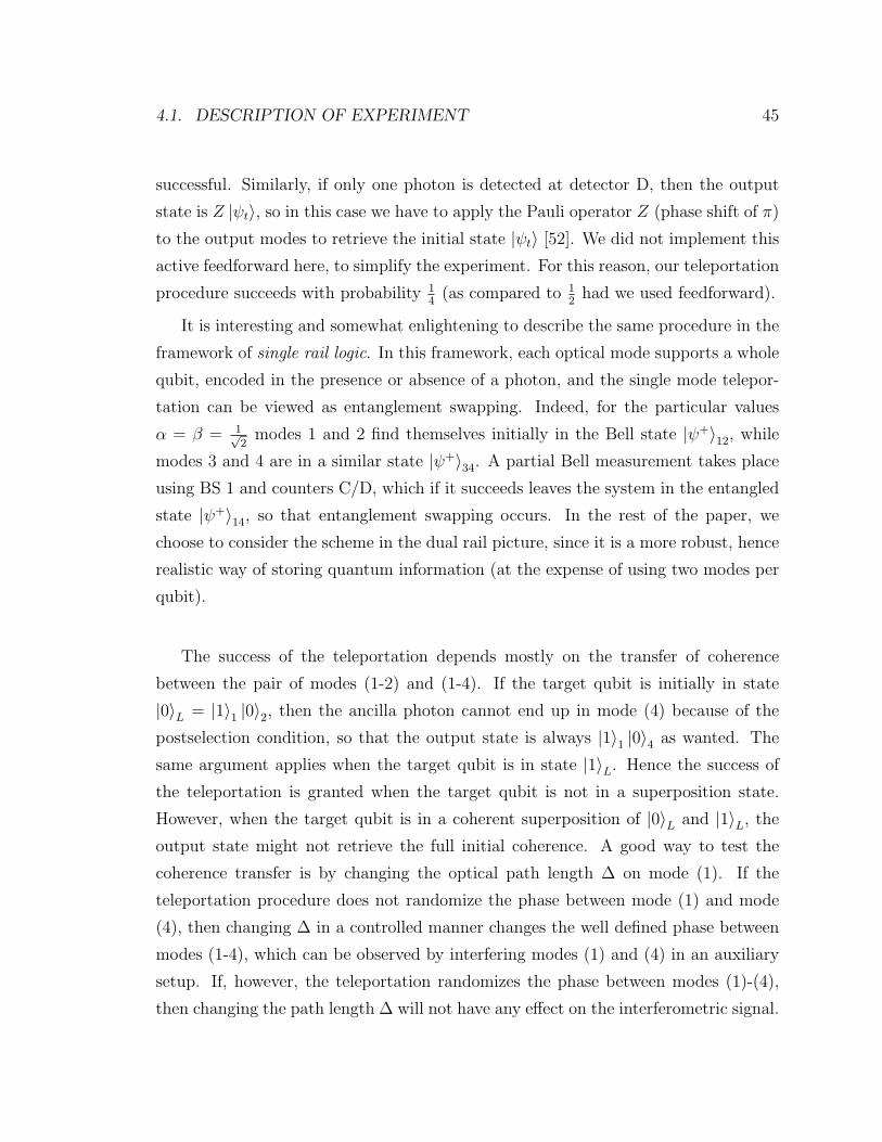
4.1. DESCRIPTION OF EXPERIMENT 45
successful. Similarly, if only one photon is detected at detector D, then the output
state is Z |ψt〉, so in this case we have to apply the Pauli operator Z (phase shift of π)
to the output modes to retrieve the initial state |ψt〉 [52]. We did not implement this
active feedforward here, to simplify the experiment. For this reason, our teleportation
procedure succeeds with probability 14
(as compared to 12
had we used feedforward).
It is interesting and somewhat enlightening to describe the same procedure in the
framework of single rail logic. In this framework, each optical mode supports a whole
qubit, encoded in the presence or absence of a photon, and the single mode telepor-
tation can be viewed as entanglement swapping. Indeed, for the particular values
α = β = 1√2
modes 1 and 2 find themselves initially in the Bell state |ψ+〉12, while
modes 3 and 4 are in a similar state |ψ+〉34. A partial Bell measurement takes place
using BS 1 and counters C/D, which if it succeeds leaves the system in the entangled
state |ψ+〉14, so that entanglement swapping occurs. In the rest of the paper, we
choose to consider the scheme in the dual rail picture, since it is a more robust, hence
realistic way of storing quantum information (at the expense of using two modes per
qubit).
The success of the teleportation depends mostly on the transfer of coherence
between the pair of modes (1-2) and (1-4). If the target qubit is initially in state
|0〉L = |1〉1 |0〉2, then the ancilla photon cannot end up in mode (4) because of the
postselection condition, so that the output state is always |1〉1 |0〉4 as wanted. The
same argument applies when the target qubit is in state |1〉L. Hence the success of
the teleportation is granted when the target qubit is not in a superposition state.
However, when the target qubit is in a coherent superposition of |0〉L and |1〉L, the
output state might not retrieve the full initial coherence. A good way to test the
coherence transfer is by changing the optical path length ∆ on mode (1). If the
teleportation procedure does not randomize the phase between mode (1) and mode
(4), then changing ∆ in a controlled manner changes the well defined phase between
modes (1-4), which can be observed by interfering modes (1) and (4) in an auxiliary
setup. If, however, the teleportation randomizes the phase between modes (1)-(4),
then changing the path length ∆ will not have any effect on the interferometric signal.

46 CHAPTER 4. SINGLE MODE TELEPORTATION
C
D
target
ancilla
output
|1
|0
|1
|1
|0
|0
BS 1
BS a
‘1’
‘4’
‘2’
‘3’
‘C’
‘D’
Figure 4.1: Schematic of single mode teleportation. Target and ancilla qubits areeach defined by a single photon occupying two optical modes (1-2 and 3-4). Whendetector C records a single photon, the state in modes 1-4 reproduces the initial stateof the target. In particular, the coherence between modes 1-2 of the target can betransferred to a coherence between modes 1-4.
4.1.3 Method
The experimental setup is shown in fig. 4.2. Two photons emitted consecutively by
the single quantum dot photon source [37, 16] are captured in a single mode fiber.
In the dual rail representation, we refer to the first photon as the ancilla, and to the
second photon as the target (see fig 4.1). The ancilla qubit, initially in state |0〉L,
is delayed in free space to match the target qubit temporally at BS 1. The delay
must be adjusted to within a fraction of the photons temporal width (∼ 200 ps or
6 cm in space). Note that the mode matching is significantly easier here than in
similar experiments using photons from PDC, where the optical path length have to
be adjusted with a tolerance of only a few microns [51].
The ancilla is prepared in the superposition state ψanc = 1√2
(|0〉L + |1〉L) with a
beam-splitter ’BS a’. The target qubit is prepared in a similar maximum superposition
state (with ’BS t’). The path length ∆ of mode (1) is changed in a controlled manner
with a piezo-actuated mirror. The ”partial Bell measurement” responsible for the
teleportation is done at BS 1 by mixing the optical modes (2) of the target qubit and
(3) of the ancilla qubit, with subsequent detection in counter C. A Mach-Zehnder
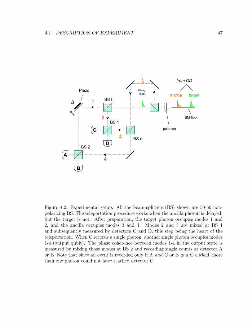
4.1. DESCRIPTION OF EXPERIMENT 47
from QD
Piezo Delayloop ancilla target
1
2 SM-fiber
D
BS 1
C
A
B
BS 2
∆ BS t
polarizer
3 BS a
4
Figure 4.2: Experimental setup. All the beam-splitters (BS) shown are 50-50 non-polarizing BS. The teleportation procedure works when the ancilla photon is delayed,but the target is not. After preparation, the target photon occupies modes 1 and2, and the ancilla occupies modes 3 and 4. Modes 2 and 3 are mixed at BS 1and subsequently measured by detectors C and D, this step being the heart of theteleportation. When C records a single photon, another single photon occupies modes1-4 (output qubit). The phase coherence between modes 1-4 in the output state ismeasured by mixing those modes at BS 2 and recording single counts at detector Aor B. Note that since an event is recorded only if A and C or B and C clicked, morethan one photon could not have reached detector C.
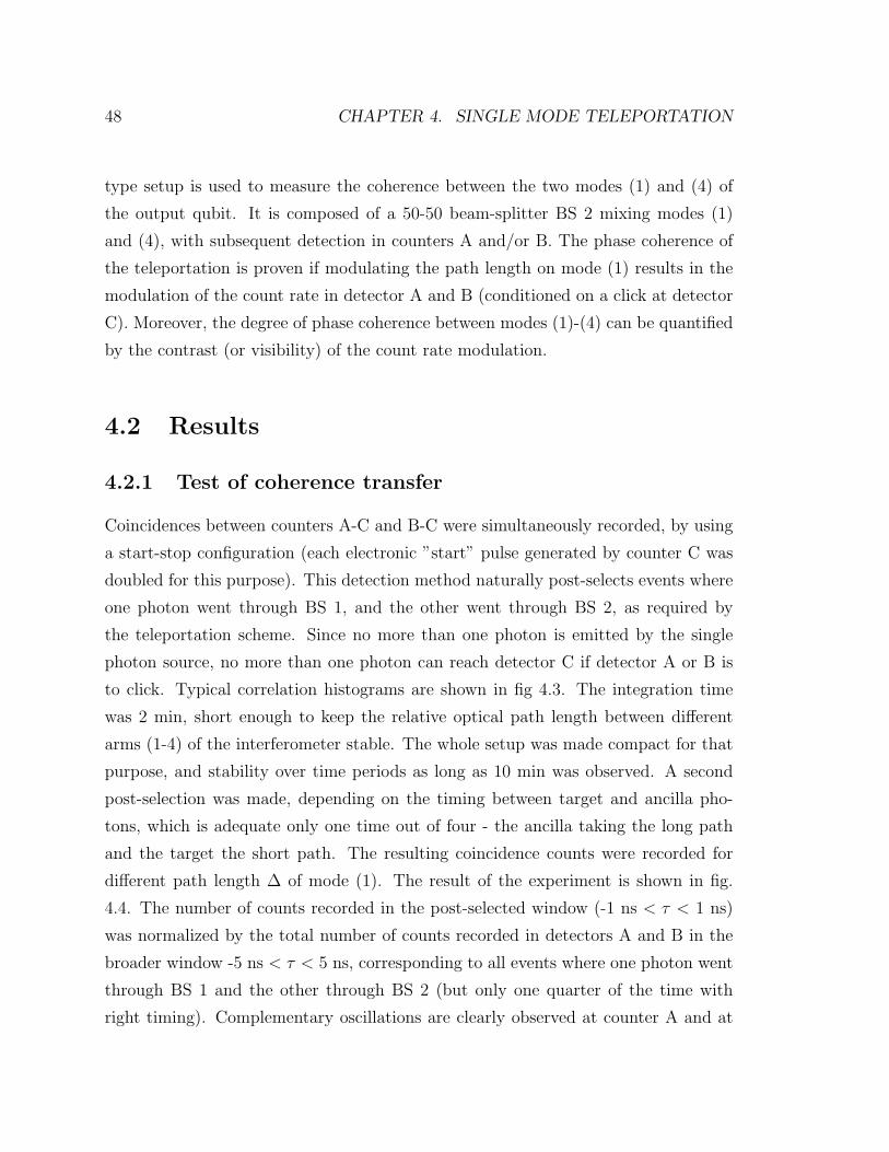
48 CHAPTER 4. SINGLE MODE TELEPORTATION
type setup is used to measure the coherence between the two modes (1) and (4) of
the output qubit. It is composed of a 50-50 beam-splitter BS 2 mixing modes (1)
and (4), with subsequent detection in counters A and/or B. The phase coherence of
the teleportation is proven if modulating the path length on mode (1) results in the
modulation of the count rate in detector A and B (conditioned on a click at detector
C). Moreover, the degree of phase coherence between modes (1)-(4) can be quantified
by the contrast (or visibility) of the count rate modulation.
4.2 Results
4.2.1 Test of coherence transfer
Coincidences between counters A-C and B-C were simultaneously recorded, by using
a start-stop configuration (each electronic ”start” pulse generated by counter C was
doubled for this purpose). This detection method naturally post-selects events where
one photon went through BS 1, and the other went through BS 2, as required by
the teleportation scheme. Since no more than one photon is emitted by the single
photon source, no more than one photon can reach detector C if detector A or B is
to click. Typical correlation histograms are shown in fig 4.3. The integration time
was 2 min, short enough to keep the relative optical path length between different
arms (1-4) of the interferometer stable. The whole setup was made compact for that
purpose, and stability over time periods as long as 10 min was observed. A second
post-selection was made, depending on the timing between target and ancilla pho-
tons, which is adequate only one time out of four - the ancilla taking the long path
and the target the short path. The resulting coincidence counts were recorded for
different path length ∆ of mode (1). The result of the experiment is shown in fig.
4.4. The number of counts recorded in the post-selected window (-1 ns < τ < 1 ns)
was normalized by the total number of counts recorded in detectors A and B in the
broader window -5 ns < τ < 5 ns, corresponding to all events where one photon went
through BS 1 and the other through BS 2 (but only one quarter of the time with
right timing). Complementary oscillations are clearly observed at counter A and at
4.2. RESULTS 49
counter B, indicating that the initial coherence was indeed transferred to the output
qubit. In other words, mode (2) of the target qubit was ”replaced” by mode (4) of
the ancilla without a major loss of coherence.
−4 −2 0 2 40
2
4
6
8
10
12
14
16
18
20
Time delay A / C (ns)
Coi
ncid
ence
cou
nts
−4 −2 0 2 40
2
4
6
8
10
12
14
16
18
20
Time delay B / C (ns)
Detector A Detector B
Figure 4.3: Typical correlation histograms taken simultaneously between detectorsA/C and B/C. The central region indicated by the dashed lines correspond to thepostselected events, when target and ancilla photons had such a timing that it isimpossible to distinguish between them based on the time of detection. As the pathlength ∆ varies, so does the relative size of the central peaks for detector A andB. The sum of count rates for the central peaks of detector A and B was 800 /s,independently of φ as shown in fig 4.4.

50 CHAPTER 4. SINGLE MODE TELEPORTATION
4.2.2 Discussion
Were the initial coherence fully conserved during the single mode transfer, the count
rate at detector A (resp. B) would be proportional to cos2(π∆λ
) (resp. sin2(π∆λ
), λ
being the single photon wavelength), giving a perfect contrast as the path length ∆ is
varied. More realistically, part of the coherence can be lost in the transfer, resulting
in a degradation of the contrast. Such a degradation is visible on fig. 4.4. It arises
mainly due to a residual distinguishability between ancilla and target photons. Slight
misalignments and imperfections in the optics also result in an imperfect mode match-
ing at BS 1 and BS 2, reducing the contrast further. Finally, the residual presence of
two-photon among pulses can reduce the contrast even more, although this effect is
negligible here. The overlap V = | 〈ψt|ψanc〉 |2 between target and ancilla wave-packets
[16], the two-photon pulses suppression factor g(2) [37], as well as the non-ideal mode
matching at BS 1 and BS 2 - characterized by the first-order interference visibilities
V1, V2 - were all measured independently. The results are V ∼ 0.75 (measured with
the setup described in [16]), g(2)(0) ∼ 2%, V1 ∼ 0.92 and V2 ∼ 0.91. The contrast C
in counts at detector A or B when we vary the phase φ should be:
C =V · V1 · V2
1 + g(2)/2∼ 0.62
This predicted value compares well with the experimental value of Cexp ∼ 0.60.
The fidelity of teleportation is F = 1+C2∼ 0.8. This high value is still not enough
to meet the requirements of efficient LOQC [46]. In particular, the quantum indis-
tinguishability of the photons must be increased further to meet these requirements.
We discussed previously the inherent limitation of our photon generation scheme for
that respect. The QD exciton from which the photon is generated dephases on a
time scale of a few nanoseconds [53], which degrades the photon indistinguishability.
Using the Purcell effect [26], one can reduce the quantum dot radiative lifetime well
below this dephasing time. However, jitter in the photon emission time will eventually
prevent any further reduction of the quantum dot lifetime. Time jitter happens as
a consequence of the incoherent character of our method to excite the quantum dot
[37]. It is currently of order 10 ps. Time jitter can be completely suppressed using a

4.2. RESULTS 51
coherent excitation technique described in great length in the next chapter (see e.g.
[54] for such a scheme with single atoms). It therefore seems vital to develop similar
techniques with single quantum dots if they are to be used for optical QIP.
0 1 2 3 4 5 6 7 80
0.05
0.1
0.15
0.2
0.25
Voltage applied to piezo (V)
prob
a of
Nor
mal
ized
coi
ncid
ence
s
Detector A
Detector B
Detector A + Detector B
Figure 4.4: Verification of single mode teleportation. Coincidence counts between de-tector A/C and B/C are plotted for different voltages applied to the piezo transducer,i.e. for different path length ∆ of mode (1). The observed modulation of the countsimplies that the initial coherence contained in the target qubit was transferred to alarge extent to the output qubit. The reduced contrast (∼ 60%) is principally due toimperfect indistinguishability between the target and ancilla photons.
Using more ancillas in a scheme first proposed in [46] and significantly improved
in [50], the single mode teleportation can be made nearly deterministic. This would
allow the replacement of deterministic non-linear gates necessary for scalable quan-
tum computation with probabilistic ones, recently demonstrated experimentally with
linear optics [47]. This generalized teleportation procedure requires more indistin-
guishable ancilla photons, produced no more than one at a time, a feature absent
in [51] but present in our implementation of the teleportation. We also point out

52 CHAPTER 4. SINGLE MODE TELEPORTATION
that the generalized scheme requires the discrimination of different photon numbers.
Progress in this direction were reported in [41], in which photon numbers up to six
could be discriminated. This would in principle allow the implementation of a linear-
optics C-z gate with a success probability of(
67
)2 ∼ 0.73 [50].
Conclusion
In conclusion, we have demonstrated the basic version of the single mode teleporta-
tion procedure described in the KLM scheme with independent single photons and
linear-optics. LOQC has emerged in recent years as an appealing alternative to pre-
vious quantum computation schemes, and to date there had been no experimental
proof of principle except for those based on parametric down conversion, a technique
that sets limits to the scalability of the system. Our experiment suggests that it is
possible to build an efficient QIP unit using single photon sources and linear-optics,
provided the photons generated are indistinguishable.

Chapter 5
Theory of coherent single photon
emission and trapping
Photons, the tiny energy wave-packets that constitute light, are almost ideal carriers
of quantum information. Single photons can in principle be produced and trapped
reversibly in matter via the interface of an optical cavity. The existing theories de-
scribing those processes are somewhat limited. They often convey the wrong ideas
that photon pulses must be relatively slow and that matter-cavity couplings must
be relatively strong in order for these processes to be efficient. Moreover it is not
precisely known which single photon pulses can be generated or trapped, a crucial
knowledge for ultra-fast operation. Here we present a general theory describing rigor-
ously when and how a single photon pulse of arbitrary known shape can be coherently
produced or trapped in a given matter-cavity system. We show that this technique
is a building block for a wide range of quantum information processes.
5.1 Background
Photons, the elementary constituents of light, are convenient carriers of quantum in-
formation since they usually barely interact with their environment. Recently, tech-
niques have been found to reversibly produce or trap photons one by one in matter.
53

54CHAPTER 5. THEORY OF COHERENT SINGLE PHOTON EMISSION AND TRAPPING
In the language of quantum information processing (QIP), these processes corre-
spond to a conversion between material and photonic qubits. This inter-conversion
capability potentially allows quantum information processes to use the best of two
worlds: the fast and reliable transport of information via photons, and its storage in
matter where interactions between qubits can be made strong. Optical cavities are
natural interface between photonic and matter qubits. They modify the structure of
the electro-magnetic field around matter, sometimes enhancing its ability to produce
or absorb light. They constitute the key element of quantum networks [14] where
matter-cavity systems called ”nodes” communicate coherently via photonic channels
[55]. It is known how to exchange or entangle the states of two identical nodes [14, ?]
in such networks via a stimulated Raman process, but only under some restrictive
conditions such as large [14] or zero [?] Raman detuning. Coherent single photon gen-
eration using the same technique [56] was demonstrated experimentally using single
atoms [57, 58, 59, 60] and single trapped ions [61], but only in the adiabatic regime
where the photon pulses are slow compared to the cavity-matter coupling constant.
Although some theoretical progress have been made recently concerning the opera-
tion in the non-adiabatic regime [?], to date it is not known which photon pulses are
eligible for trapping or emission in a given node. In this chapter, we give a rigorous
answer to that open question. We derive a single criterion (5.1) on the time-varying
amplitude of a single photon pulse, which determines whether this pulse can be re-
versibly trapped and/or generated in a given node. We show that the restrictions
previously made to understand the dynamics of these systems, such as adiabaticity,
strong coupling, large or zero detuning, symmetry between emitting and trapping
sites are not necessary and reduce to special cases of the present theory. Given an
arbitrary photon pulse that satisfies criterion (5.1), the present theory explain how to
drive the node with a classical ”control” light pulse so that it will trap the incident
photon or release it in a controlled, coherent fashion. Although the present theory
makes no assumption on the physical implementation of a node, we specifically have
in mind a semiconductor quantum dot (QD) loaded with a single electron placed in a
photonic crystal resonator [62]. In this particular system, the present theory opens up
the perspective of coherent emission and trapping of ultra-fast single photons, with

5.2. SUMMARY OF RESULTS 55
temporal width as short as a few picoseconds with current technology [63, ?]. The
chapter first describes the core results on photon trapping and emission for ideal sys-
tems, then evaluates the performance of these processes under realistic experimental
conditions. Finally, it gives a number of important applications for ultra-fast and
reliable quantum information processing.
Figure 5.1: Simulation of a high Q micro-cavity coupled to a single waveguide trans-verse mode realized in a 2D photonic crystal. a) Structure used for simulation. b)Map of the energy density on a linear scale. The light contained in the confinedcavity mode leaks on the left in a single wave-guide mode. c) Map of the magneticfield amplitude. d) Map of the energy density on a logarithmic scale.
5.2 Summary of results
For the sake of clarity, we give in this section a summary of the main results of our
theory of photon trapping. The mathematical details of the claims made here will be
given in a further section.
5.2.1 General theory
Much like classical light pulses that are produced in lasers, single photon pulses
can have many different spatio-temporal profiles. Under certain general conditions

56CHAPTER 5. THEORY OF COHERENT SINGLE PHOTON EMISSION AND TRAPPING
explained in the first chapter, they are described by photo-detection probability am-
plitudes [?] that we call ”photon pulse amplitude”. Photons emitted through the
fluorescence of an excited 2-level system [19, 37, 21, 22, 18] like those used in the
experiments of chapters 3 and 4 have an amplitude which is a one-sided decaying
exponential. Photon pulses with more singular shapes have been produced recently,
by driving single 3-level atoms [58] or ions [61] into a stimulated raman adiabatic
passage (STIRAP) [56]. These first realizations of coherent single photon production
use quantum systems in a Λ configuration, with two ground states |e〉, |g〉 and an
excited state |r〉. This will be the starting point of our analysis. Consider the system
shown in Fig. (5.2). A quantum emitter with non-degenerate ground states |e〉 and
|g〉 and excited state |r〉 is located in a one-sided optical micro-cavity. We will refer
to this joint system as a ”node”. The |r〉 to |g〉 dipole transition is nearly resonant
with the field of a single cavity mode (resonance frequency ωc), with a vacuum Rabi
frequency g0. The cavity mode is coupled to an external radiation field, with energy
decay rate denoted by κ. We control a classical laser pulse with center frequency ωL
nearly resonant with the |e〉 − |r〉 dipole transition, and with a coherent Rabi fre-
quency Ω(t). We assume that the control pulse and the cavity resonance have same
detuning ∆ relative to their respective transition.
Suppose a single photon pulse with amplitude α(t)e−iωct is incident on the node,
which is initialized in state |g〉. The complex photon pulse envelope α(t) is known,
and we want to design a control pulse Ω(t) so that the node completely absorbs the
incident photon and ends up in state |e, 0〉 deterministically. The main result of this
section is that this absorption process can be done perfectly if and only if the photon
pulse satisfies the following condition for all times:
E(t) ≡∫ t
−∞|α(s)|2ds− |α(t)|2
κ− 1
κg20
|α− κ
2α(t)|2 > 0 (5.1)
This relation tells us qualitatively that the single photon bandwidth cannot be
much greater than κ, and that g0 cannot be much smaller than κ. However in general,
it does not require an often-assumed adiabaticity condition (| αα| << g0), nor does it
require the regime of strong coupling (g0 >> κ). We also learn that the detuning of

5.2. SUMMARY OF RESULTS 57
(control pulse) (cavity)
Λ system
Cavity mode
(arbitrary single photon pulse)
Figure 5.2: Composition of a ”node”: 3-level atom or quantum dot in a Λ configu-ration placed in a single mode optical micro-cavity. The g-r transition frequency isclose to the incident photon and cavity resonance, and has a vacuum Rabi frequencyg0 with the cavity mode. The e-r transition couples to a classical laser pulse called”control pulse”. This transition does not couple to the cavity, due to polarization orfrequency mismatch for instance. The cavity mode, mathematically represented byannihilation operator a, is coupled to an external radiation mode, which gives it afinite decay rate κ. It is assumed that the cavity can exchange energy solely withthat particular external mode.
the photon pulse relative to the cavity frequency can be as large as g0. The proof
leading to relation (5.1) is given in a following section.
When this relation holds, we can always design a control pulse Ω(t) that enforces
a destructive interference between two photon amplitudes: one being reflected by the
front mirror of the cavity and the other being absorbed and re-emitted by the system
(see Fig. 5.3). As a result, there is no net reflection of the incident photon. The
absolute value of the required control pulse needs to be:
|Ω(t)
2| =|α− (κ
2− i∆)α + (g2
0 − i∆κ2)α(t)|√
κg20E(t)
(5.2)
The control pulse must in general have a chirp to compensate both for a possible
chirp in the incident photon pulse and for an eventual finite detuning ∆. The exact
expression for the chirp is rather complicated, and can be found in the supplementary
material. However if the photon envelope has no chirp, and if ∆ = 0, the control pulse

58CHAPTER 5. THEORY OF COHERENT SINGLE PHOTON EMISSION AND TRAPPING
Figure 5.3: Physical picture of the photon trapping process. In words, the incomingphoton wave-packet can escape the node in two distinct ways: by direct reflection onthe cavity front mirror (solid green line) or by absorption and re-emission from theatom-cavity system (dashed green line). If the control pulse applied to the Λ system iswell designed, the probability amplitudes for these two events interfere destructively,and the photon stays trapped in the atom-cavity system with a probability of one.
does not need to have a chirp and is given by the simple expression, also derived in
[?] although not in closed form :
Ω(t)
2=α− κ
2α + g2
0α(t)√κg2
0E(t)(5.3)
The solution to the photon trapping problem also gives a solution to the photon
emission problem after time-reversal. This means that ultra-fast single photon pulses
can be produced deterministically, provided they obey the time-reversed relation (5.1).
Relation (5.1) generally implies that arbitrary single photon pulses can be perfectly
emitted or trapped as long as they are not detuned from the cavity resonance ωc by
more than g0, and as their bandwidth γp does not exceed Min(κ,
g20
κ
). This is true
even in the weak coupling regime (g0 << κ). In the strong or intermediate coupling
regimes, these processes can be made as fast as the cavity decay rate κ, in which
case the control pulse becomes highly non-adiabatic and must be precisely designed
to match the corresponding photon envelope. In the large detuning case, which was
studied earlier in [14] , relation (5.1) can only be satisfied in the strong coupling

5.2. SUMMARY OF RESULTS 59
regime, and the control pulse shape is given by:
|g0Ω(t)
2∆| =
|α− κ2α(t)|√
κ∫ tinfty|a(s)|2ds− |α(t)|2
(5.4)
We write the result in this form since g0Ω(t)2∆
is the effective Raman coupling between
the two ground states |e〉 and |g〉 after adiabatic elimination of level |r〉. Additionally,
if the incident photon has no chirp, the control pulse must have a necessary chirp Φ(t)
given by :
Φ(t) = −|Ω(t)|2
4∆(5.5)
Relations (5.4-5.5) agree with and extend the results of [14], where identical nodes
and time-reversal invariant photon shapes were assumed. The necessary chirp of the
control pulse can be interpreted as a cancellation of the AC stark-shift induced by
level |r〉 or level |e〉 via the classical control pulse.
Another limit of interest is the adiabatic regime, where the incident (emitted)
photon pulse is slow enough so that γp Min[κ,
g20
κ
]. This is the regime in which
existing coherent single photon sources are operated. If we further assume ∆ = 0,
the control pulse has no chirp and takes the simple form:
Ω(t)
2=
g0√κ
α(t)√∫ t−∞ |a(s)|2ds
(5.6)
Note that the denominator is the square root of the total energy carried by the
photon up to time t, and absorbed by the cavity. Therefore, the intensity |Ω(t)|2 of
the control pulse is proportional to the instantaneous rate at which the single photon
energy enters the cavity. This result is pretty intuitive: it means that any energy
accumulated in level |g〉 from the radiation mode must be immediately transferred to
level |e〉, otherwise it will be re-radiated and lost. Equation (5.6) can be expressed
equivalently as:

60CHAPTER 5. THEORY OF COHERENT SINGLE PHOTON EMISSION AND TRAPPING
α(t) =
√κ
g0
Ω(t)
2exp
[κ
2g20
∫ t
−∞|Ω(s)
2|2ds
](5.7)
which gives the photon shape if we know the (adiabatic) control pulse. This
result explains previous experimental observations and simulations of coherent photon
emission via the STIRAP technique [58, 61]. In the adiabatic regime, the emitted
photon pulse follows the control pulse except for a slight correction given by the
exponential term in Eq. (5.7), causing the emitted photon pulse to raise slower and
decay faster than the control pulse.
5.2.2 Real systems: performance analysis
Whereas many experimental systems implementing the present schemes can be found
with stable ground states |e〉 and |g〉, they will usually suffer from the decay of a
cavity photon into spurious modes, as well as from finite longitudinal decay and
dephasing rates of the excited level |r〉. A proper study of these effects would require
a master equation method, but here get estimates assuming that they cause only
a small perturbation on the system dynamics, which can be checked a posteriori.
Spurious cavity losses will affect the overall efficiency of the scheme. If Gammac
denotes the total rate of such losses, assumed small compared to κ, both the trapping
and emission schemes suffer from a reduction Lc of efficiency given by:
Lc ∼ Γc
∫ ∞−∞|g(t)|2dt =
Γcκ
(5.8)
Spontaneous decay from level |r〉 at rate γ further reduces the efficiency of the
schemes and can degrade the quantum mechanical overlap between two photons emit-
ted consecutively [16]. The reduction of efficiency L due to γ can be estimated to
be :
L ∼ γ
∫ ∞−∞|r(s)|2ds =
γ
g20
[κ
4+
1
κ
∫ ∞−∞|α(s)|2ds
](5.9)
and for most valid photon shapes, does not exceed γκ2g2
0. In the photon emission
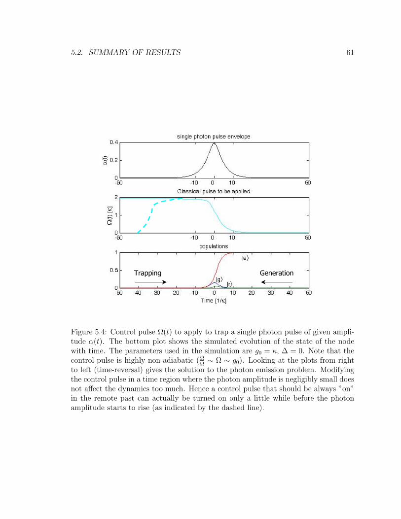
5.2. SUMMARY OF RESULTS 61
Trapping Generation
Figure 5.4: Control pulse Ω(t) to apply to trap a single photon pulse of given ampli-tude α(t). The bottom plot shows the simulated evolution of the state of the nodewith time. The parameters used in the simulation are g0 = κ, ∆ = 0. Note that thecontrol pulse is highly non-adiabatic ( Ω
Ω∼ Ω ∼ g0). Looking at the plots from right
to left (time-reversal) gives the solution to the photon emission problem. Modifyingthe control pulse in a time region where the photon amplitude is negligibly small doesnot affect the dynamics too much. Hence a control pulse that should be always ”on”in the remote past can actually be turned on only a little while before the photonamplitude starts to rise (as indicated by the dashed line).

62CHAPTER 5. THEORY OF COHERENT SINGLE PHOTON EMISSION AND TRAPPING
Trapping Generation
Figure 5.5: Generation and trapping of a single photon pulse with oscillating ampli-tude. The conditions are also very non-adiabatic. The shape of the control pulse isnot really intuitive...
case, if level |r〉 decays spontaneously to level |e〉, emitted photons will have fluctuat-
ing shapes and their mean overlap O will be reduced. (If α1(t) and α2(t) are the ampli-
tudes of two photons, their overlap O is defined as the quantity∣∣∣∫∞−∞ α1(t)α∗2(t)dt
∣∣∣2).
It can be shown however that:
O > 1− 2γ
∫ ∞−∞|r(s)|2ds > 1− γκ
2g20
(5.10)
and this bound is very loose. Dephasing of level |r〉 at rate Γd can also reduce
the overlap between consecutive photons (by a factor as large as 2Γdγp
) and, to a much
lesser extent, the overall efficiency of the scheme. Note that the effect of losses and
noise due to the transit through level |r〉 are greatly reduced in the strong coupling
regime. Interestingly, even in the intermediate or weak coupling regimes, these effects

5.2. SUMMARY OF RESULTS 63
Trapping Generation
Figure 5.6: Deterministic photon trapping/generation deep in the weak couplingregime. The parameters are g0
κ= 0.1, ∆ = 0. The photon pulse cannot be as fast
as in the intermediate (or strong) coupling case (upper limit on bandwidth isg20
κ
instead of κ). Level |r〉 is also significantly more populated, causing increased lossby spontaneous emission (∼ 22 γ
κhere if small loss) and degradation of consecutive
photon overlap. These undesired effects could still be small in a realistic QD-cavitysystem with κ ∼ 1/1ps, g0 ∼ 1/10ps and γ ∼ 1/1ns for instance, where the quantumefficiency would be 98% and overlap greater than 95%.

64CHAPTER 5. THEORY OF COHERENT SINGLE PHOTON EMISSION AND TRAPPING
can be small if the Purcell factor 4g02γκ
is much greater than 1. This is the case of QD
- cavity systems fabricated by many many groups today [63, 64, 65, ?].
Therefore, a large vacuum Rabi frequency g0 is not necessary for the scheme
to work even in the presence of realistic experimental imperfections. This coher-
ent scheme can reduce the impact of dephasing and finite lifetime of level |r〉, and
achieves a high generation efficiency and quantum indistinguishability. Applications
to quantum information processing and quantum optics The scheme described above
has important applications in the field of photonic quantum information processing.
We will mention some of these applications in increasing order of complexity. We
will give figures assuming that a node is made of a semiconductor quantum dot in
a photonic crystal cavity, coupled to a photonic crystal wave-guide. We will use the
following values that are realistic for what can be achieved today in several labs : γ ∼1/1 ns, κ ∼ 1/ 10 ps, g0 ∼ 1/ 10 ps.
5.3 Applications
In this section, we give a (non-exhaustive) list of applications of the photon trap-
ping/generation technique to the processing of quantum information. We show how
this technique alone is a building block to perform arbitrary quantum computation.
5.3.1 Single photon generation
The coherent photon-trapping scheme presented here allows the deterministic gener-
ation of single photon pulses with duration as short as k−1 even in the intermediate
coupling regime (and κg20
in the weak-coupling regime). With the currently available
quantum dot - photonic crystal cavity technology [63, 64, 65, ?], single photon pulses
with temporal width of a few picoseconds could be reliably produced, with no time-
jitter, generation efficiency greater than 99%, and quantum mechanical overlap of
two consecutive photons as high as 98%. These figures could be further improved by
increasing the vacuum Rabi frequency g0 and the cavity decay rate κ with respect
to g. A new feature predicted by the present theory is the complete control of the

5.3. APPLICATIONS 65
photon pulse amplitude α(t), as long as the condition (5.1) is satisfied. This feature
of temporal pulse shape control capability, illustrated in Figs 3 and 4, gives access
to a new degree of freedom to store and manipulate quantum information in single
photon pulses, never exploited in the past. An immediate application is a differential
phase shift quantum key distribution (DPSQKD) protocol, based on single photon
pulses [66]. This protocol requires single photon pulses that are linear superpositions
of elementary pulses well separated in time, with random 0 or π phase shifts between
them. An example with two elementary pulses with relative phase shift of π is given
on Fig. 5.7.
Trapping Generation
Figure 5.7: Generation and trapping of a composite single photon pulse for differentialphase shift QKD. The pulse is a superposition of two elementary pulses well separatedin time and with a π phase shift between them.

66CHAPTER 5. THEORY OF COHERENT SINGLE PHOTON EMISSION AND TRAPPING
5.3.2 Non-destructive single photon detection
The photon trapping technique can be used for the non-destructive detection of a
single photon of known temporal profile. Whether a photon is incident or not, we
apply a trapping control pulse to a node in state |g〉. If and only if a photon is present,
the node makes the transition to state |e〉. We can then measure the state of the node
in a non-destructive way, e.g. by bouncing a coherent light pulse with frequency ω
well detuned from the node resonance wc and measuring the resulting small phase
shift. After the node measurement, the single photon can be re-emitted with a same
or different temporal profile. If the control pulse is chosen to produce an identical
pulse shape, the scheme realizes a quantum non-demolition measurement. If the
control pulse is chosen to produce a different pulse shape, the scheme realizes a single
photon pulse shape transformer. This method provides a single-photon detection with
efficiency exceeding 99% and negligible dark counts.
5.3.3 Formation of quantum entanglement between nodes
This can simply be realized by simultaneous trapping of a split single photon pulse
in two different nodes, as shown on Fig. (5.8). A single photon can be split in a
beam-splitter with reflection coefficient r and transmission coefficient t, which can be
implemented as a branching circuit of a photonic crystal wave-guide. After trapping,
the nodes are left in the entangled state r|ge〉 + t|eg〉. By using a 1 to N branching
circuit to split the initial photon pulse, we can similarly create a large multi-partite
entangled state - a W state [67] of size N.
5.3.4 Non-destructive parity measurement for two nodes
We consider the geometry shown in Fig. 5b. A coherent light pulse |β > is sent on
a 50/50% beam-splitter. The split pulses bounce simultaneously on the two nodes.
Each pulse acquires either zero or finite phase shift φ, depending on the state of the
nodes. The two pulses interfere on their way back to the beam-splitter. A photon
number measurement on one of the output ports of the beam-splitter projects the
joint state of the nodes onto their even or odd parity subspace, depending on whether
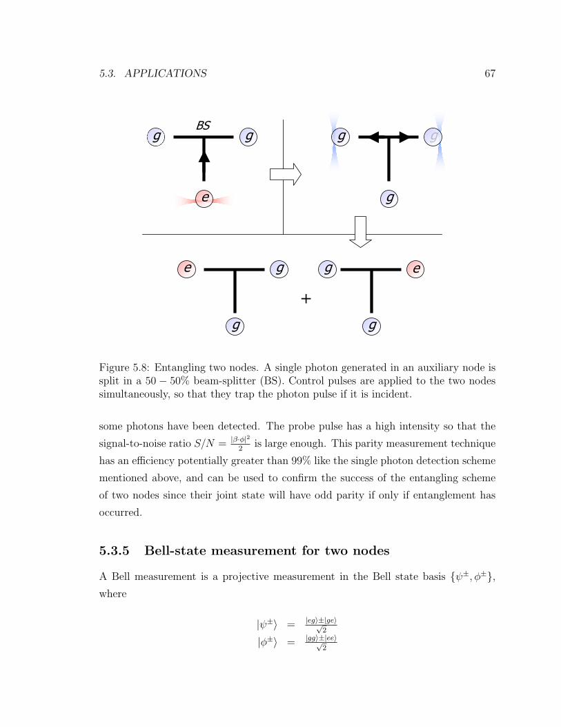
5.3. APPLICATIONS 67
e
g g g gBS
g
+
e eg
g
g
g
Figure 5.8: Entangling two nodes. A single photon generated in an auxiliary node issplit in a 50 − 50% beam-splitter (BS). Control pulses are applied to the two nodessimultaneously, so that they trap the photon pulse if it is incident.
some photons have been detected. The probe pulse has a high intensity so that the
signal-to-noise ratio S/N = |β·φ|22
is large enough. This parity measurement technique
has an efficiency potentially greater than 99% like the single photon detection scheme
mentioned above, and can be used to confirm the success of the entangling scheme
of two nodes since their joint state will have odd parity if only if entanglement has
occurred.
5.3.5 Bell-state measurement for two nodes
A Bell measurement is a projective measurement in the Bell state basis ψ±, φ±,where
|ψ±〉 = |eg〉±|ge〉√2
|φ±〉 = |gg〉±|ee〉√2

68CHAPTER 5. THEORY OF COHERENT SINGLE PHOTON EMISSION AND TRAPPING
x
x
y
xBS
Figure 5.9: Non-destructive measurement of the parity of two nodes. A coherent lightpulse |β〉 is sent in a 50−50% BS. The split pulses bounce simultaneously off the twoand recombine at the beam-splitter. Measuring the photon number at an open portof the beam-splitter, the state of the two nodes is projected onto their even (|gg〉 or|ee〉) or odd (|ge〉 or |eg〉) subspace. The probability of error in this measurement canbe made arbitrarily small by increasing the magnitude |β| of the probe beam.
This measurement can be realized as a succession the parity measurement de-
scribed above and the sign measurement that distinguishes the same parity group
apart. We first consider the odd parity case. The sign measurement for the odd par-
ity subspace ψ± can be realized with the same network geometry as for the parity
measurement. We apply simultaneous generation control pulses to the two nodes,
then a single photon emission occurs if the node was in state |e〉. Since the nodes
were in odd parity, exactly one photon is released in the system. The two wave-guides
from the nodes cross in a 50−50% beam-splitter, and a photon number measurement
is performed on the two output ports. Depending on the measurement result, that
is, at which port a single photon exits, we learn the sign ε of the initial node state|eg〉+ε|ge〉√
2.
If the parity of the nodes was first measured even, we can perform the sign mea-
surement as follows. We first flip the state of one node, exchanging the |e〉 and |g〉component of the state. This operation can be realized by a σx Pauli gate of the
node, using an effective π pulse for the Raman transition via level |r〉. This operation
swaps the odd and even parity subspaces and also adds an excess phase factor i. The
sign measurement can be done for the odd parity subspace.

5.3. APPLICATIONS 69
BS
Figure 5.10: Sign measurement within odd parity subspace. Simultaneous emissioncontrol pulses are applied to the nodes. The resulting split photon pulse recombines ina BS and a photon number measurement is performed on the two outputs. Dependingon the side where the click occurs, the two nodes are measured in the Bell state ψ+
or ψ−.
5.3.6 Non-linear interaction of single photons
Suppose two single photons, a ”control” and a ”target”, are sent sequentially on a
node in an initial state |g, 0〉. A trapping control pulse is applied, which translates
the node state to |e, 0〉. The target photon then sees an empty cavity. As shown
in the mathematical section below, if the temporal duration of the photon is larger
than 1κ, the target photon is reflected off the cavity without distortion but with a π
phase shift. The control photon can then be re-emitted in the transmission line. Now
suppose the control photon was absent. Then the target photon sees a node in state
|g, 0〉, and is also reflected off with no distortion but this time with no phase shift.
Therefore, the presence of the control photon induces a π phase shift on the target
photon. This constitutes a control-Z gate between two photonic qubits in the dual
rail representation.
5.3.7 Full QIP with electronic qubits
Suppose we encode the information in the two ground states of a node. In the
quantum dot scheme that we have in mind, these states correspond to the ”spin up”
and ”spin down” of a single electron in the QD. One qubit operation can be performed
by individually addressed Raman pulses, creating an effective coupling between the
|e〉 and |g〉 levels via level |r〉 (charged exciton state). A simple procedure allows to

70CHAPTER 5. THEORY OF COHERENT SINGLE PHOTON EMISSION AND TRAPPING
perform a control-Z operation between two nodes A and B if they are linked by the
photonic channel. First apply a generating control pulse to node A, which releases a
photon in the channel if (and only if) node A was in state |e〉. The photon reflects off
node B and acquires a π phase shift if (and only if) node B is in state |e〉. Apply a
trapping control pulse to node A to capture back the photon on its way back. After
this procedure, the joint system (A,B) has acquired a π phase shift if and only if both
nodes A and B were in state |e〉, which is the realization of a control-Z operation.
In other words, the two nodes interacted via a controlled exchange of a photon.
Since we also described above a (non-destructive) technique to measure the state of a
single node, we can claim that full quantum computation is in theory possible in this
system. In particular, the ability to accurately manipulate and measure the state of
individual network nodes together with the relative easiness to perform a Control-Z
gate between two nodes make of this system an ideal candidate to implement a fast
one-way quantum computer [68].
5.3.8 Discussion
We presented a cavity QED technique for coherent photon trapping and generation
that has important and immediate applications for quantum information. It pro-
vides total control over a single photon pulse amplitude, and therefore a new way to
encode quantum information with immediate application in quantum cryptography.
The ability to reversibly store photonic qubits in matter where a Bell measurement
can be easily implemented is particularly attractive for the realization of a quan-
tum repeaters [69]. Looking more in the future, the present technique would allow a
hybrid form of quantum computation in a network architecture, particularly compat-
ible with photonic crystal technology. The nodes of the network, acting as quantum
register storing qubits, could interact by the exchange of photons through the pho-
tonic crystal wave-guide. Quantum information could also be reversibly transferred
to single photons in the single or dual rail qubit form, manipulated individually by
linear optics elements [46] such as beam-splitters with adjustable ratio (implemented

5.3. APPLICATIONS 71
BA
A B
A B
Figure 5.11: Control-Z operation between two electronic qubits (A,B). We apply agenerating control pulse followed by a trapping control pulse to node A. A singlephoton travels in the wave-guide if and only if node A was in state |e〉. Also a singlephoton reflecting off node B acquires a π phase shift if and only if node B is in state|e〉. Therefore the joint system (A,B) acquires a global π phase shift if and only iffound in state |ee〉.

72CHAPTER 5. THEORY OF COHERENT SINGLE PHOTON EMISSION AND TRAPPING
as ultra-fast photonic switches [70]). This concept of on-chip cavity QED network ar-
chitecture integrate a universal quantum computation system together with quantum
communication channels and linear-optics information processing circuits.
5.4 Mathematical details of the theory.
The purpose of this section is to give a mathematical proof of the main result of
the photon trapping theory, namely that given an incident single photon pulse with
complex amplitude α(t) satisfying Eq. (5.1), there is a corresponding control pulse
Ω(t) = |Ω(t)eiΦ(t)| to be applied to the |r〉 − |e〉 transition that will allow perfect
trapping of the photon pulse.
5.4.1 System dynamics
The photon pulse α(t) is incoming on a one-sided cavity with decay rate κ. We assume
the photon is in a spatial travelling mode perfectly matched with a single confined
mode of the cavity, described by annihilation operator a. Inside the cavity, there is a
Λ-type quantum system, with two metastable states |g〉 and |e〉 and an excited state
|r〉. The transition |g〉 − |r〉 is coupled to the vacuum field of the confined cavity
mode, with vacuum Rabi frequency g0. The |r〉 − |e〉 transition is coupled to the
control pulse Ω(t). We will assume an ideal system where none of the levels decay by
spontaneous emission.
The output field of the cavity is related to the input field and the confined field
by the following relation [71] in the Heisenberg picture :
ain(t) + aout(t) =√κa(t) (5.11)
This relation makes the implicit assumption that the coupling of the cavity mode
to different longitudinal modes of the wave-guide is the same in a range of frequency
κ around the cavity resonance. This condition might not be satisfied for photonic

5.4. MATHEMATICAL DETAILS OF THE THEORY. 73
crystal structures unless designed carefully (e.g. one wants to avoid coupling near the
wave-guide band-edge). The Heisenberg equation of motion for the cavity mode a is :
da
dt= i[HΛ, a]− κ
2a+√κain (5.12)
The first term represent the coherent evolution of the confined field due to its
coupling to the Λ system. The second and third terms are damping and associated
”noise” due to its coupling with the continuum of radiative modes of the cavity -
where the photon comes from.
We treat the coupled atom-cavity system as an entity called a ”node”, interacting
with the external radiation field. We define a non-normalized wave-function Ψ(t) for
the excited node, i.e. for a node that has absorbed a photon:
Ψ(t) = g(t) |g, 1〉+ r(t) |r, 0〉+ e(t) |e, 0〉 (5.13)
where |X,n〉 represents the state X of the Λ system and the number n of photon
inside the cavity.
The state Ψ(t) evolves according to:
g = −ig0 r −κ
2g +√κα(t) (5.14)
r = −i∆r − ig0 g − iΩ
2e (5.15)
e = −iΩ∗
2r (5.16)
where we used the rotating-wave approximation. The carrier frequency for the
photon pulse is taken to be ωc, the resonant frequency of the cavity. We assumed
that the two-photon resonance condition is satisfied, and ∆ is the common detuning
of the laser and cavity field from the excited level |r〉.

74CHAPTER 5. THEORY OF COHERENT SINGLE PHOTON EMISSION AND TRAPPING
5.4.2 Impedance matching
From the last set of equations, one can show that :
|g|2(t) + |r|2(t) + |e|2(t) =
∫ t
−∞|α(s)|2 ds−
∫ t
−∞|√κg(s)− α(s)|2 ds (5.17)
This quantity represents the energy absorbed in the atom-cavity system from the
incoming photon pulse, up to time t. Note that it depends on the detuning implicitly
through the amplitude g(t). We therefore always have the intuitive result that :
|g|2(t) + |r|2(t) + |e|2(t) ≤∫ t
|α|2(s) ds (5.18)
Moreover, the inequality is strict unless :
∀s,√κ g(s) = α(s) (5.19)
If (and only if) the relation (5.19) is satisfied, the system absorbs the photon
perfectly, and is left in state |e, 0〉. Indeed as t→ +∞, α(t)→ 0, therefore g(t)→ 0.
Then in virtue of relation (5.14), r(t)→ 0. Then e(t)→∫∞−∞ |α(s)|2 ds = 1.
The condition (5.19) for perfect trapping can be seen as an impedance matching
condition and has a nice physical interpretation. If we apply equation (5.11) to the
initial state |Ψ0〉 of the system, and re-adopt the state varying (Schrodinger) picture,
we find that :
〈vac| aout(t) |Ψ0〉 =(√
κg(t)− α(t))
(5.20)
Then if the impedance matching condition is satisfied, there is simply no light
coming out of the cavity. The quantum amplitude of the photon pulse being directly
reflected off the front cavity mirror and that of the photon being absorbed then re-
emitted from the node interfere destructively at all times, so that the absorption is
perfect.
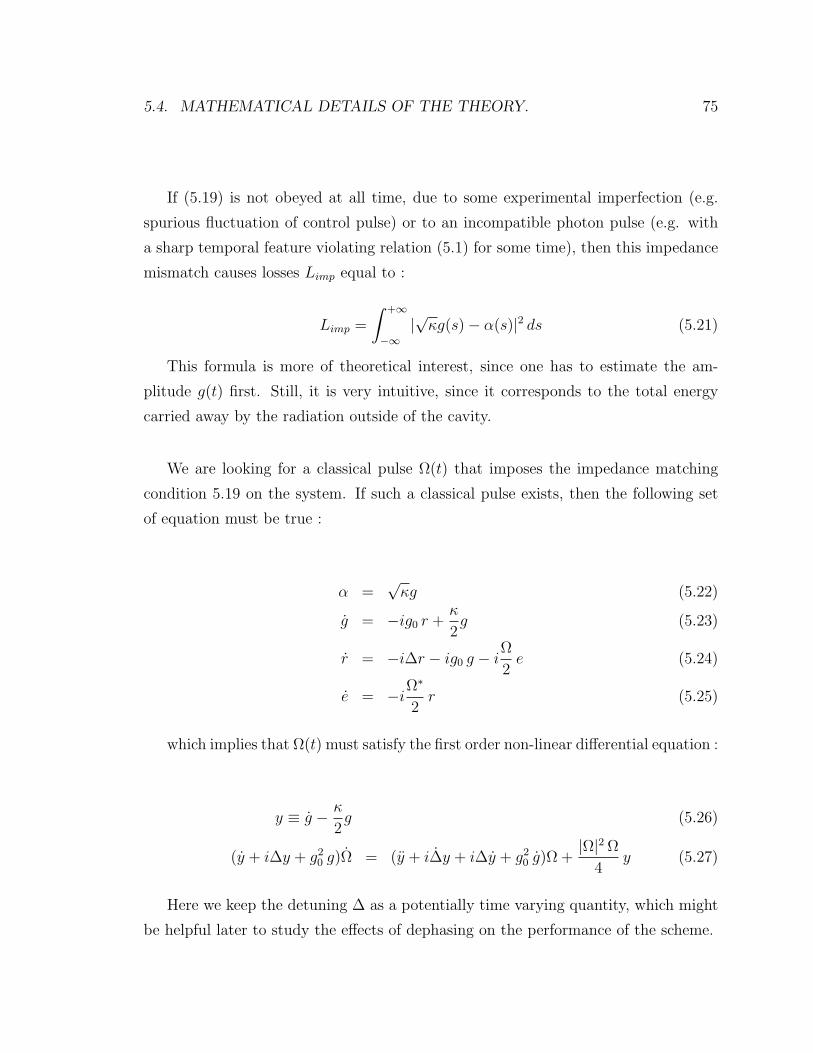
5.4. MATHEMATICAL DETAILS OF THE THEORY. 75
If (5.19) is not obeyed at all time, due to some experimental imperfection (e.g.
spurious fluctuation of control pulse) or to an incompatible photon pulse (e.g. with
a sharp temporal feature violating relation (5.1) for some time), then this impedance
mismatch causes losses Limp equal to :
Limp =
∫ +∞
−∞|√κg(s)− α(s)|2 ds (5.21)
This formula is more of theoretical interest, since one has to estimate the am-
plitude g(t) first. Still, it is very intuitive, since it corresponds to the total energy
carried away by the radiation outside of the cavity.
We are looking for a classical pulse Ω(t) that imposes the impedance matching
condition 5.19 on the system. If such a classical pulse exists, then the following set
of equation must be true :
α =√κg (5.22)
g = −ig0 r +κ
2g (5.23)
r = −i∆r − ig0 g − iΩ
2e (5.24)
e = −iΩ∗
2r (5.25)
which implies that Ω(t) must satisfy the first order non-linear differential equation :
y ≡ g − κ
2g (5.26)
(y + i∆y + g20 g)Ω = (y + i∆y + i∆y + g2
0 g)Ω +|Ω|2 Ω
4y (5.27)
Here we keep the detuning ∆ as a potentially time varying quantity, which might
be helpful later to study the effects of dephasing on the performance of the scheme.

76CHAPTER 5. THEORY OF COHERENT SINGLE PHOTON EMISSION AND TRAPPING
5.4.3 Control pulse design
We want to show that the impedance matching condition can be insured by choosing
a control pulse Ω(t) satisfying the relation (5.27) if there exists one. If we can indeed
find such a pulse, then the following equations are true :
x ≡ g − α√κ
(5.28)
x = −ig0 r −κ
2x (5.29)
r = −i∆r − ig∗0 x− iΩ∗
2e (5.30)
e = −iΩ2r (5.31)
This can be seen as the photon trapping problem where the amplitude of state |g〉is now the quantity x, and where the photon pulse vanishes at all time. The solution
to that problem is trivial: x must vanish at all time. In other words, if we can find a
solution Ω(t) to equation (5.27) defined for all times, then perfect trapping will occur.
Luckily, we can find a closed form solution for (5.27). First we define :
z ≡ Ω
y + i∆y + g20 g
= − 2
g0e(t)(5.32)
Equation (5.27) can then be changed into :
4z
|z|2 z= yy∗ − i∆|y|2 + g2
0 yg∗ (5.33)
Now writing z = ρeiθ, we get :
4ρ
ρ3=
1
2
d
dt|y|2 +
g20
2
d
dt|g|2 − g2
0
κ
2|g|2 (5.34)
4θ
ρ2= Im
[y(y∗ + g2
0g∗)]−∆|y|2 (5.35)

5.4. MATHEMATICAL DETAILS OF THE THEORY. 77
From there, we want to obtain an expression for Ω(t) depending only on α(t). We
will write α(t) = |α(t)|eiβ(t) and will denote ξ(t) ≡˙|α||α| the instant rate of variation
of the photon pulse envelope. Using the initial condition that e(−∞) = 0, we obtain
the result :
Ω(t)
2=
1
g0
√κe(t)
[α− κ
2a+ g2
0α + i∆(α− κ
2α)]
(5.36)
|e(t)|2 =
∫ t
−∞|α(s)|2ds− |α(t)|2
κ[1 +
(ξ − κ2)2
g20
+β2
g20
] (5.37)
d
dtArg[e(t)] =
|α(t)|2
κg20|e(t)|2
[∆[(ξ − κ
2)2 + β2] + β[(ξ − κ
2)2 − g2
0 − ξ] (5.38)
+β(ξ − κ
2)]
This solution is defined if and only if the right hand side of Eq. (5.37) is positive
at all times, which is the criterion (5.1) announced earlier. If this is true, then |Ω(t)|is bounded on any compact time interval and therefore is a maximal solution of the
non-linear equation (5.27) for all times in virtue of the Cauchy-Lipschitz theorem [72].
Large detuning case
This is the regime where ∆ κ, g0,∣∣∣dlog(α)
dt
∣∣∣ , |Ω|, ∣∣∣dlog(Ω)dt
∣∣∣. In this case level |r〉 has
negligible population, and can be adiabatically eliminated from the dynamics, re-
ducing the 3-level problem to a simpler 2-level one, with an effective laser induced
coupling Ωeff (t) = g0 Ω(t)∆
. In such a case, the trapping control pulse must be :∣∣∣∣Ω(t)
2
∣∣∣∣ =|∆||α− κ
2α|√
κg20
∫ t−∞ |α(s)|2ds− g2
0|α(t)|2 − |α− κ2α|2
(5.39)
The condition that ∆ Ω implies that :
|α− κ
2α|2 κg2
0
∫ t
−∞|α(s)|2ds− g2
0|α(t)|2 ∀t (5.40)
which can in general be satisfied only in the regime of strong coupling where

78CHAPTER 5. THEORY OF COHERENT SINGLE PHOTON EMISSION AND TRAPPING
g0 κ. This is because roughly speaking, Ω∆∼ κ
g0. In the strong coupling regime, we
can write : ∣∣∣∣Ωeff (t)
2
∣∣∣∣ =|α− κ
2α|√
κ∫ t−∞ |α(s)|2ds− |α(t)|2
(5.41)
Note that Ωeff will not have an amplitude much greater than κ. Additionally, the
control pulse must have a necessary chirp given by :
Φ(t) = β(t) + Arctan
(β
ξ
)−∫ t
−∞
|Ω(t)|2
4∆(5.42)
which reduces to the simpler relation :
Φ = −|Ω|2
4∆(5.43)
if the photon pulse itself has no chirp. This last relation can be simply interpreted
as a compensation of the AC Stark shift created by the far detuned control pulse on
the e-r transition.
In this large detuning regime, fast photon pulses can still be trapped or emitted,
the bandwidth being limited by the cavity decay κ only. However, strong coupling is
necessary.
Zero detuning case
The control pulse must have amplitude :
|Ω(t)
2|2 =
∣∣α− κ2α + g2
0α∣∣2
κg20
∫ t−∞ |α(s)|2ds− g2
0|α(t)|2 − |α− κ2α|2
(5.44)
Moreover, if the photon pulse has no chirp, then neither does Ω(t). Also we don’t
need to be in strong coupling anymore for the denominator to be positive. Perfect

5.4. MATHEMATICAL DETAILS OF THE THEORY. 79
trapping can occur even if g0 ∼ κ. These two facts are important advantages com-
pared to the large detuning case.
If the photon pulse to trap is slow (| αα| κ) and if we are in the strong coupling
regime g0 κ, we get a simplified result :
∣∣∣∣Ω(t)
2
∣∣∣∣2 ∼ g20|α(t)|2∫ t
−∞ |α(s)|2 ds(5.45)
So in a sense, the control pulse and photon pulse follow each other. After differ-
entiating relation (5.45), we can obtain the dual result :
|α(t)|2 =κ
g20
∣∣∣∣Ω(t)
2
∣∣∣∣2 e κ
2g20
∫+∞t |Ω(s)
2|2 ds
(5.46)
which can be convenient to compare the shape of the envelopes of the control and
photon pulse. This result explains previous experimental observations and simulations
of coherent photon emission via the STIRAP technique [58, 61]. In the adiabatic
setting used in these experiments, the emitted photon pulse ”follows” the control
pulse except for a slight correction given by the exponential term in eq. (5.46),
causing the emitted photon pulse to raise slower and decay faster in time than the
control pulse.
5.4.4 Reflection of a single photon pulse off a passive node
In our proposal for a Control-Z operation between distant nodes of a quantum net-
work, we claimed that a single photon pulse could be reflected off a node without
distortion and with a phase shift depending on the state of the node. Here we prove
that assertion and state the conditions under which it is valid.
When no control pulse is applied to the node, level |e > is decoupled from levels
|g〉 and |r〉. Suppose a single photon pulse αin(t) is incident on the node in state e.
In the Heisenberg picture, we have the following dynamics:

80CHAPTER 5. THEORY OF COHERENT SINGLE PHOTON EMISSION AND TRAPPING
a = −κ2
a +√κain (5.47)
which after Fourier transform gives:
a(ω) =
√κ
−iω + κ2
ain(ω) (5.48)
Together with the input-output cavity relation (5.11), we obtain:
aout(ω) =iω + κ
2
−iω + κ2
ain(ω) (5.49)
If the photon pulse is slow compared to κ, we get the approximate result :
aout(t) ∼ ain(t− 4
κ) (5.50)
which means that the pulse is reflected with no phase shift and a small time shift 4κ.
If we start with the node in state |g >, the relevant dynamics is :
g = −κ2g − ig0r +
√καin (5.51)
r = −ig0g (5.52)
After Fourier transform, and use of relation (5.11) we obtain :
αout(ω) =iω κ
2+ ω2 + g2
0
iω κ2− ω2 − g2
0
αin(ω) (5.53)
If the photon pulse is slow compared to κ, we get the approximate result :
αout(t) ∼ −αin(t− κ
g20
) (5.54)
This time the pulse is reflected with a π phase shift and a time shift of κg20
(this
result is valid only for a single photon input). The time shift is deterministic and can
be corrected later if desired. It becomes negligible in the regime of strong coupling.

Chapter 6
Conclusion and prospects
We summarize below the main achievements of the thesis :
Demonstration of single and indistinguishable photon emission with a
Quantum Dot in a micropillar structure
We demonstrated the generation of single photons from Quantum dots in micropillar
cavities, with a large suppression of multi-photon pulses. We observed the bunching
effect of two identical photons ”colliding” in a beam-splitter.
Entanglement formation between two independent single photons
We used the micropillar structures to produce sequentially two independent single
photon pulses. We used a linear-optical trick to entangle these photons upon photo-
detection. We observed the violation of Bell’s inequality, and characterized the full
joint polarization state of the entangled photons.
Quantum teleportation of an optical dual-rail qubit
We used the micropillar structures once more to generate two optical qubits, a target
to be teleported and an ancilla to be measured in the teleportation process. This
process is a building block of linear-optics quantum computation.
81

82 CHAPTER 6. CONCLUSION AND PROSPECTS
Fabrication and optical characterization of photonic bandgap cavities
Photonic bandgap cavities promise better performance than micropillar cavities. We
developed a fabrication method for 2D photonic crystal membranes, with a crystal
defect acting as a high Q and small mode volume micro-cavity.
Investigation of single quantum dot/ PBG cavity coupling
We observed both the enhancement and suppression of spontaneous emission of a
single QD exciton in a photonic bandgap cavity, corresponding to Purcell factors
ranging from 10 to 0.2.
General theory of coherent single photon generation and trapping
We presented the theory of a coherent cavity QED technique to reversibly trap or
generate single photon pulses or arbitrary shape in a 3-level quantum system with a
Λ configuration.
Proposal of QIP with QD electron spin interacting via a photonic crystal
channel
We showed how the single photon trapping technique can be used to perform a full
Bell state measurement and a conditional phase shift operation between two electron
spins contained in distant quantum dots.
Some experimental projects attempted during the thesis have not given satisfac-
tory results, and will be passed on a new generation of students. These projects
include :
• Generation of polarization-entangled photon pairs from a QD bi-exciton.
• Convincing evidence of strong coupling between a QD exciton and a single PBG
cavity mode.

83
Future prospects
Ongoing experimental efforts in our labs are directed toward the realization of a co-
herent single photon source. This implies the ability to load a single electron in a
QD to create two distinct ground states, and apply a transverse magnetic field of a
few tesla to artificially re-create a Λ system via a charged exciton state (trion). The
precise control of the photon pulse shape will involve equally precise design of the
control laser pulse shape.
In the longer term, our collaboration wants to develop of a full quantum network
system made of single QDs in photonic crystal cavities, communicating via the ex-
change of single photons through photonic crystal waveguides. The single electron
spin carrying the information in a node could even be reversibly transferred to the
nuclear spin of In atoms contained in the QD and protected by externally applied
Nuclear-Magnetic-Resonance pulses.
The development of quantum networks will be facilitated by clever design of pho-
tonic crystal cavity and waveguide, and especially of the interface between the two.
Progress in that direction are made almost everyday thanks to the ingenuity of their
authors relying on 2D or 3D FDTD simulations to guide their intuition.

Appendix A
Theory of Quantum Dot-cavity
coupling
It is hard to find in the literature an comprehensive treatment of the simple problem
of a 2-level system decaying through the single mode of an optical cavity. In this
appendix, we precisely tackle this problem. These calculations were performed as
an attempt to explain the experimental spectra of single QD decaying in photonic
crystal single mode cavities.
Formulation of problem
A 2-level system in its excited state decays in a finite Q single-mode cavity. After
we wait long enough, a single photon will be found in either of these two radiative
continuum : the α-continuum representing the radiation of the cavity mode, or the
β-continuum representing the radiation through leaky modes. We want to know what
fraction of the light actually decays through the cavity, and what is its spectrum.
Solution
We consider the system shown in Fig. A.1. A two-level system with energy separation
ω0 is coupled to a (flat) continuum of (locally) uniform density Dβ, as well as to a
84

85
…
continuum αcontinuum βdensity Dαdensity Dβ
2-level system
cavitysingle mode
Figure A.1: Description of the coupled emitter-cavity system.
single cavity mode. The cavity, resonant at ωc, is itself coupled to a (flat) contin-
uum of uniform density Dα. We define the spontaneous emission rate of the 2-level
system into the β-continuum as γ and the (energy) decay rate of the cavity into the
α-continuum as κ. Note that γ can differ from the free space spontaneous emission
rate, because the cavity changes the structure of the vacuum around the emitter. A
Wigner-Weisskopf type calculation shows that the coupling of the 2-level system to
the β-continuum around the resonant frequency ω0 must be B0 ≡√
γ2πD0
β, and that
the coupling of the cavity to the α-continuum near the resonance frequency ωc must
be Ac ≡√
κ2πDcα
(this can be done by solving equations (2−5) with the emitter-cavity
coupling turned off). The emitter’s coupling to the empty cavity mode is defined asg2, where g is usually called the vacuum Rabi frequency of the emitter-cavity system.
Since there is a single quantum in the system, its state at all times can be written
as:
|ψ(t)〉 = a(t) |e, 0c, 0α, 0β〉+b(t) |g, 1c, 0α, 0β〉+∑α
cα(t) |g, 0c, 1α, 0β〉+∑β
dβ(t) |g, 0c, 0α, 1β〉 .
(A.1)

86 APPENDIX A. THEORY OF QUANTUM DOT-CAVITY COUPLING
The Schrodinger equation idψdt
= Hψ then simplifies to the following set of equa-
tions:
d a
dt= −ig
2ei(ω0−ωc)t b− i
∑β
Bβ ei(ω0−ωβ)t dβ (A.2)
d b
dt= −ig
∗
2e−i(ω0−ωc)t a− i
∑α
Aα ei(ωc−ωα)t cα (A.3)
d cαdt
= −i A∗α ei(ωα−ωc)t b (A.4)
d dβdt
= −i B∗β ei(ωβ−ω0)t a (A.5)
with initial conditions:
a(0) = 1
b(0) = cα(0) = dβ(0) = 0
We solve those equations using Laplace transforms. The Laplace transform of a
function f(t) is defined as:
f(s) ≡∫ ∞
0
e−stf(t) dt (A.6)
with inverse transform:
f(t) =1
2iπ
∫ ε+i∞
ε−i∞estf(s) ds (A.7)
The Laplace transform of equations A.5 gives the equivalent set of equations:
sa(s)− 1 = −i g2b(s− i(ω0 − ωc))− i
∑β
Bβ dβ(s− i(ω0 − ωβ)) (A.8)
sb(s) = −ig∗
2a(s+ i(ω0 − ωc))− i
∑α
Aα cα(s− i(ωc − ωα)) (A.9)
scα(s) = −i A∗α b(s− i(ωα − ωc)) (A.10)
sdβ(s) = −i Bβ a(s− i(ωβ − ω0)) (A.11)

87
From this set of equations, we get:
a(s) =
[s+|g|2
4
1
s− i(ω0 − ωc) +∑
α|Aα|2
s−i(ω0−ωα)
+∑β
|Bβ|2
s− i(ω0 − ωβ)
]−1
(A.12)
b(s) = −i g∗
2
a(s+ i(ω0 − ωc))s+
∑α
|Aα|2s+i(ωα−ωc)
(A.13)
cα(s) = −i A∗αb(s− i(ωα − ωc))
s(A.14)
dβ(s) = −i B∗βa(s− i(ωβ − ω0))
s(A.15)
The function c(s) has three poles, but two of them describe the transient temporal
behavior (strictly negative real part). The long time population of the α-continuum
is described by the s = 0 pole of c(s):
cα(t→∞) = lims→0+
−i A∗αb(s− i(ωα − ωc)) (A.16)
To perform this limit, we need to compute terms similar to lims→0+
∑α
|Aα|2s−i(ω0−ωα)
.
Using∑
α ∼∫Dαdωα, and the well-know result from distribution theory :
lims→0+
1
x+ is= P(
1
x)− iπδ(x), (A.17)
we obtain the result :
lims→0+
∑α
|Aα|2
s− i(ω0 − ωα)=κ
2+ (Lamb shift) (A.18)
and similarly,
lims→0+
∑β
|Bβ|2
s− i(ω0 − ωβ)=γ
2+ (Lamb shift) . (A.19)
The principal part (Lamb Shift or energy renormalization) gives an imaginary contri-
bution that we embed in the definition of the physical resonances of the system (as
compared to the bare resonances). We finally obtain the main result of those notes,

88 APPENDIX A. THEORY OF QUANTUM DOT-CAVITY COUPLING
namely the asymptotic amplitudes of the states in the α-continuum:
cα(t→∞) =AαAc
√κ
2πDcαg/2
(ωα − ωc + iκ2)(ωα − ω0 + iγ
2)− |g|2
4
(A.20)
where Dcα is the density of the α-continuum around frequency ωc . Similarly, the
asymptotic amplitudes of the leaky mode states (β-continuum) are:
dβ(t→∞) =Bβ
B0
√γ
2πD0β
ωβ − ωc + iκ2
(ωβ − ωc + iκ2)(ωβ − ω0 + iγ
2)− |g|2
4
. (A.21)
The total probability of decay into the α-continuum, assuming a reasonably flat
structure, is
Pcav =∑
α |cα(t→∞)|2
u∫Dα|cα(t→∞)|2 dωα
= |g|2κ8π
∫dωα
(ωα−ω1)(ωα−ω∗1)(ωα−ω2)(ωα−ω∗2)
In the above expression, ω1 and ω2 are the poles of cα(t→∞) viewed as a function
of ωα. They can be compactly written as
ω1 =ω0 + ωc
2+
1
2
√(ω0 − ωc)2 + |g|2 (A.22)
ω2 =ω0 + ωc
2− 1
2
√(ω0 − ωc)2 + |g|2 (A.23)
where ω0 = ω0 − iγ2and ωc = ωc − iκ
2. The reader can check (I did !) that they
both have negative imaginary parts under all circumstances. Then using the residue
theorem, we easily get:
Pcav =|g|2κ8π
π
|ω1 − ω∗2|2
∣∣∣∣ 1
Im(ω1)+
1
Im(ω2)
∣∣∣∣ (A.24)
Before we give the result of the integration, we give some intermediate results.
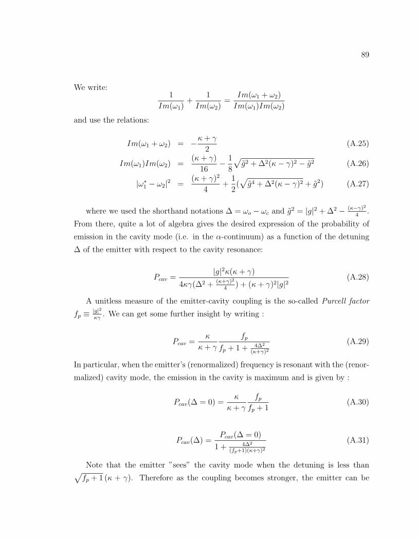
89
We write:1
Im(ω1)+
1
Im(ω2)=
Im(ω1 + ω2)
Im(ω1)Im(ω2)
and use the relations:
Im(ω1 + ω2) = −κ+ γ
2(A.25)
Im(ω1)Im(ω2) =(κ+ γ)
16− 1
8
√g2 + ∆2(κ− γ)2 − g2 (A.26)
|ω∗1 − ω2|2 =(κ+ γ)2
4+
1
2(√g4 + ∆2(κ− γ)2 + g2) (A.27)
where we used the shorthand notations ∆ = ωo − ωc and g2 = |g|2 + ∆2 − (κ−γ)2
4.
From there, quite a lot of algebra gives the desired expression of the probability of
emission in the cavity mode (i.e. in the α-continuum) as a function of the detuning
∆ of the emitter with respect to the cavity resonance:
Pcav =|g|2κ(κ+ γ)
4κγ(∆2 + (κ+γ)2
4) + (κ+ γ)2|g|2
(A.28)
A unitless measure of the emitter-cavity coupling is the so-called Purcell factor
fp ≡ |g|2κγ
. We can get some further insight by writing :
Pcav =κ
κ+ γ
fp
fp + 1 + 4∆2
(κ+γ)2
(A.29)
In particular, when the emitter’s (renormalized) frequency is resonant with the (renor-
malized) cavity mode, the emission in the cavity is maximum and is given by :
Pcav(∆ = 0) =κ
κ+ γ
fpfp + 1
(A.30)
Pcav(∆) =Pcav(∆ = 0)
1 + 4∆2
(fp+1)(κ+γ)2
(A.31)
Note that the emitter ”sees” the cavity mode when the detuning is less than√fp + 1 (κ + γ). Therefore as the coupling becomes stronger, the emitter can be

90 APPENDIX A. THEORY OF QUANTUM DOT-CAVITY COUPLING
more detuned from the cavity resonance and still emit in the cavity mode.
ω – ωc
Figure A.2: Radiation spectrum from the cavity mode for various coupling strengths.The emitter is resonant with the cavity mode.

91
ω – ωc
Figure A.3: Leaky modes spectrum when emitter is on resonance with cavity.

Bibliography
[1] Rarity et al. Quantum Random-Number Generation and Key Sharing. Journal
of Modern Optics, 41:2435–2444, 1994.
[2] R.P. Feynman. Simulating Physics with Computers. International Journal of
Theoretical Physics, 21:467–488, 1982.
[3] I.L. Chuang and M.A. Nielsen. Quantum Computation and Quantum Informa-
tion. Cambridge University Press, 2000.
[4] P.W. Shor. Algorithms for quantum computation: discrete logarithms and factor-
ing, Proceedings 35th Annual Symposium on Foundations of Computer Science.
IEEE Comput. Soc. Press, Santa Fe, NM, USA, 1994.
[5] A. Kitaev. Quantum measurements and the Abelian stabilizer problem. quant-
ph/9511026, 1995.
[6] L.K. Grover. A Fast Quantum Mechanical Algorithm for Database Search. Pro-
ceedings of the 28th Annual ACM Symposium on the Theory of Computing, pages
212–219, 1996.
[7] D. Bimberg, M. Grundmann, and N.N. Ledentsov. Quantum Dot Heterostruc-
tures. John Wiley & Sons, Chichester, 1999.
[8] W.K. Wootters and W.H. Zurek. A Single Quantum Cannot be Cloned. Nature,
299:802–803, 1982.
[9] W.H. Zurek. Decoherence, Einselection, and the Quantum Origins of the Clas-
sical. Reviews of Modern Physics, 75:715–775, 2003.
92

BIBLIOGRAPHY 93
[10] D. Loss and D.P. DiVincenzo. Quantum computation with quantum dots. Phys.
Rev. A, 57:120, 1998.
[11] H.J. Briegel, T. Calarco, D. Jaksch, J.I. Cirac, and P. Zoller. Quantum computing
with neutral atoms. Journal of Modern Optics, 47:415451, 2000.
[12] J.I. Cirac and P. Zoller. Quantum Computations with Cold Trapped Ions. Phys.
Rev. Lett., 74:40914094, 1995.
[13] Y. Nakamura, Y.A. Pashkin, and J.S. Tsai. Coherent control of macroscopic
quantum states in a single-Cooper-pair box. Nature, 398:786, 1999.
[14] J.I. Cirac, P. Zoller, H.J. Kimble, and H. Mabuchi. Quantum state transfer and
entanglement distribution among distant nodes in a quantum network. Phys.
Rev. Lett., 78:3221–3224, 1997.
[15] C. Cohen-Tannoudji, J. Dupont-Roc, and G. Grynberg. Photons and Atoms -
Introduction to Quantum Electrodynamics. John Wiley & Sons, 1989.
[16] C. Santori, D. Fattal, J. Vuckovic, G.S. Solomon, and Y. Yamamoto. Indistin-
guishable photons from a single-photon device. Nature, 419:594–597, 2002.
[17] V.A. Shchukin, N.N. Ledentsov, P.S. Kop’ev, and D. Bimberg. Spontaneous
ordering of arrays of coherent strained islands. Physical Review Letters, 75:2968,
1995.
[18] Z. Yuan et al. Electrically driven single-photon source. Science, 295:102–105,
2002.
[19] P. Michler et al. A quantum dot single-photon turnstile device. Science,
290:2282–2285, 2000.
[20] C. Santori, M. Pelton, G.S. Solomon, Y. Dale, and Y. Yamamoto. Triggered
single photons from a quantum dot. Phys. Rev. Lett., 86:1502–1505, 2001.
[21] V. Zwiller et al. Single quantum dots emit single photons at a time: antibunching
experiments. Appl. Phys. Lett., 78:2476–2478, 2001.

94 BIBLIOGRAPHY
[22] E. Moreau et al. Single-mode solid-state single photon source based on isolated
quantum dots in pillar microcavities. Appl. Phys. Lett., 79:2865–2867, 2001.
[23] R. Heitz et al. Multiphonon-relaxation processes in self-organized InAs/GaAs
quantum dots. Applied Physics Letters, 68:361, 1996.
[24] F. Adler et al. Optical transiitons and carrier relaxation in self-assembled
InAs/GaAs quantum dots. Journal of Applied Physics, 80:4019, 1996.
[25] E. M. Purcell. Spontaneous emission probabilities at radio frequencies. Physical
Review, 69:681, 1946.
[26] J. Vuckovic, M. Pelton, A. Scherer, and Y. Yamamoto. Optimization of three-
dimensional micropost microcavities for cavity quantum electrodynamics. Phys-
ical Review A, 66:052208, 2002.
[27] M. Pelton, J. Vuckovic, G. S. Solomon, A. Scherer, and Y. Yamamoto. Three-
dimensionally confined modes in micropost microcavities: Quality factors and
Purcell factors. IEEE Journal of Quantum Electronics, 38(2):170–177, 2002.
[28] C. Santori. Generation of non-classical light using semicinductor quantum dots.
Ph. D. Thesis, Stanford University, 2002.
[29] J. M. Gerard, B. Sermage, B. Gayral, B. Legrand, E. Costard, and V. Thierry-
Mieg. Enhanced spontaneous emission by quantum boxes in a monolithic optical
microcavity. Physical Review Letters, 81:1110–1113, 1998.
[30] C.H. Bennett and D.P. DiVicenzo. Quantum information and computation. Na-
ture, 404:247–255, 2000.
[31] D. Bouwmeester, J.W. Pan, K. Mattle, M. Eibl, H. Weinfurter, and A. Zeilinger.
Experimental quantum teleportation. Nature, 390:575–579, 1997.
[32] Y.H. Shih and C.O. Alley. New type of Einstein-Podolsky-Rosen-Bohm experi-
ment using pairs of light quanta produced by optical parametric down conversion.
Physical Review Letters, 61:2921–2924, 1988.

BIBLIOGRAPHY 95
[33] Z.Y. Ou and L. Mandel. Violation of Bell’s inequality and classical probability in
a two-photon correlation experiment. Physical Review Letters, 61:50–53, 1988.
[34] J.-W. Pan, D. Bouwmeester, H. Weinfurter, and A. Zeilinger. Experimental
Entanglement Swapping: Entangling Photons That Never Interacted. Physical
Review Letters, 80:3891–3894, 1998.
[35] J.-W. Pan, M. Daniell, S. Gasparoni, G. Weihs, and Anton Zeilinger. Experi-
mental Demonstration of Four-Photon Entanglement and High-Fidelity Telepor-
tation. Physical Review Letters, 86:44354438, 2001.
[36] A. Peres. Separability Criterion for Density Matrices. Physical Review Letters,
77:1413–1415, 1996.
[37] C. Santori, M. Pelton, G. Solomon, Y. Dale, and Y. Yamamoto. Triggered single
photons from a quantum dot. Physical Review Letters, 86(8):1502–1505, 2001.
[38] S. Popescu, L. Hardy, and M. Zukowski. Revisiting Bell’s theorem for a class of
down-conversion experiment. Physical Review A, 56:R4353, 1997.
[39] J.F. Clauser, M.A. Horne, A. Shimony, and R.A. Holt. Proposed Experiment to
Test Local Hidden-Variable Theories. Physical Review Letters, 23:880, 1969.
[40] A. G. White, D. F. V. James, P. H. Eberhard, , and P. G. Kwiat. Nonmaxi-
mally Entangled States: Production, Characterization, and Utilization. Physical
Review Letters, 83:3103–3107, 1999.
[41] S. Takeuchi, J. Kim, Y. Yamamoto, and H. Hogue. Development of a high-
efficiency single-photon counting system. Applied Physics Letters, 74:1063, 1999.
[42] A.K. Ekert. Quantum cryptography based on Bell’s theorem. Physical Review
Letters, 67:661–663, 1991.
[43] C. H. Bennett, G. Brassard, and N. D. Mermin. Quantum cryptography without
Bell’s theorem. Physical Review Letters, 68:557–559, 1992.

96 BIBLIOGRAPHY
[44] E. Waks, A. Zeevi, and Y. Yamamoto. Security of quantum key distribution with
entangled photons against individual attacks. Physical Review A, 65:052310,
2002.
[45] T. C. Ralph, A. G. White, W. J. Munro, and G. J. Milburn. Simple scheme for
efficient linear optics quantum gates. Phys. Rev. A, 65:12314, 2002.
[46] E. Knill, R. Laflamme, and G. J Milburn. A scheme for efficient quantum com-
putation with linear optics. Nature, 409:46–52, 2001.
[47] T.B. Pitman, M.J. Fitch, B.C. Jacobs, and J.D. Franson. Experimental
controlled-not logic gate for single photons in the coincidence basis. Quant-
ph/0303095, 2003.
[48] D.Gottesman and I.L.Chuang. Demonstrating the viability of universal quantum
computation using teleportation and single-qubit operations. Nature, 402:390,
1999.
[49] C.H. Bennett, G. Brassard, C. Crpeau, R. Jozsa, A. Peres, and W.K. Wootters.
Teleporting an unknown quantum state via dual classical and Einstein-Podolsky-
Rosen channels. Physical Review Letters, 70:1895–1899, 1993.
[50] J.D. Franson, M.M. Donegan, M.J. Fitch, B.C. Jacobs, and T.B. Pitman. High-
fidelity quantum logic operations using linear optical elements. Phys. Rev. Lett.,
89:137901, 2002.
[51] E. Lombardi, F. Sciarrino, S. Popescu, and F. DeMartini. Teleportation of a
VacuumOne-Photon Qubit. Phys. Rev. Lett., 88:070402, 2002.
[52] S. Giacomini, F. Sciarrino, E. Lombardi, and F. De Martini. Active teleportation
of a quantum bit. Phys. Rev. A, 66:030302, 2002.
[53] D. Fattal, C. Santori, J. Vuckovic, G.S. Solomon, and Y. Yamamoto. Indis-
tinguishable single photons from a quantum dot. Phys. Stat. Sol (b), 238:305,
2003.
BIBLIOGRAPHY 97
[54] A. Kuhn, M. Heinrich, and G. Rempe. Deterministic single-photon source for
distributed quantum networking. Physical Review Letters, 89:067901, 2002.
[55] S.J. Van Enk, J.I. Cirac, and P. Zoller. Photonic channels for quantum commu-
nication. Science, 279:205–208, 1998.
[56] A. Kuhn, M. Hennrich, T. Bondo, and G. Rempe. Controlled generation of single
photons from a strongly coupled atom-cavity system. Appl. Phys. B, 69:373–377,
1999.
[57] M. Hennrich, T. Legero, A. Kuhn, and G. Rempe. Vacuum-stimulated Raman
scattering based on adiabatic passage in a high finesse optical cavity. Phys. Rev.
Lett., 85:4872–4875, 2000.
[58] A. Kuhn, M. Hennrich, and G. Rempe. Deterministic single-photon source for
distributed quantum networking. Phys. Rev. Lett., 89:67901, 2002.
[59] J. McKeever et al. Determisnistic generation of single photons from one atom
trapped in a cavity. Science, 303:1992–1994, 2004.
[60] S. Brattke, B.T. Varcoe, and H. Walther. Generation of photon number states
on demand via cavity quantum electrodynamics. Science, 86:3534–3537, 2001.
[61] M. Keller, B. Lange, K. Hayasaka, W. Lange, and H. Walther. Continuous gen-
eration of single photons with controlled waveform in an ion-trap cavity system.
Nature, 431:1075–1078, 2004.
[62] A. Kiraz, M. Atature, and A. Imamoglu. Quantum dot single photon sources:
prospects for application in linear-optics quantum information processing. Phys.
Rev. A, 69:032305, 2004.
[63] T. Yoshie et al. Vacuum Rabi splitting with a single quantum dot in a photonic
crystal nanocavity. Nature, 432:200–203, 2004.
[64] J.P. Reithmaier et al. Strong coupling in a single quantum dot - semiconductor
microcavity system. Nature, 432:197–200, 2004.
98 BIBLIOGRAPHY
[65] E. Peter et al. Exciton photon strong-coupling regime for a single quantum dot
in a microcavity. quant-ph/0411076, 2004.
[66] K. Inoue, E. Waks, and Y. Yamamoto. Differential phase shift quantum key
distribution. Phys. Rev. Lett., 89:37902, 2002.
[67] W. Dur, G. Vidal, and I.J. Cirac. Three qubits can be entangled in two different
ways. Phys. Rev. A, 62:62314, 2000.
[68] R. Raussendorf and H.J. Briegel. A one-way quantum computer. Phys. Rev.
Lett., 86:5188–5191, 2001.
[69] H.J. Briegel, W. Dur, J.I. Cirac, and P. Zoller. Quantum repeater: The role of
imperfect local operations in quantum communication. Phys. Rev. Lett., 81:5932–
5935, 1998.
[70] H. Nakamura et al. Ultra-fast photonic crystal/ quantum dot all-optical switch
for future photonic networks. Optics express, 12:6606–6614, 2004.
[71] D.F. Walls and G.J. Milburn. Quantum Optics. Springer-Verlag, Berlin, 1994.
[72] F. Laudenbach. Calcul differentiel et integral. Editions de l’Ecole Polytechnique,
2000.


