Download - Singular Two Points Boundary Value Problem
An-Najah National University
Faculty of Graduate Studies
Singular Two Points
Boundary Value Problem
By
Sawsan Mohammad Hamdan
Supervised by
Dr. Samir Matar
This thesis is submitted in partial fulfillment of the requirements for the
Degree of Master in Computational Mathematics, Faculty of Graduate
Studies at An-Najah National University, Nablus, Palestine
2010


III
Dedication
To My Parents, My Husband, My children Raghad, Saif Al-deen, Mayar, My
Sisters, Brothers, and to the Soul of the martyr Ihsan and to all who helped
me to fulfill this thesis, I dedicate it.

IV
Acknowledgments
First, my greatest thanks for allah for helping me finish this work as good as
I hope.
Then my all thanks and wishes for my supervisor Dr. Samir Matar who
directed me to finish this research successfully.
Dr. Mohammad N. Ass'ad who supported and helped me to be one of
researcher students and granted me his trust.
Finally, my all thanks and wishes for my mother, father and husband
especially, for their help and encouragement, and to my friends for all kinds
of support and concern.
V
Singular Two Points
Boundary Value Problem
Declaration
The work provided in this thesis, unless otherwise referenced, is the
researcher's own work, and has not been submitted elsewhere for any other
degree or qualification.
Student's name:
Signature:
Date:
VI
Table Of CONTENTS
Declaration V
List Of Tables VIII
List of Figures IX
Abstract X
Chapter 1: Introduction
1.1 Introduction 2
1.2 Differential Equation 3
1.3 Ordinary Differential equations 4
1.4 Initial Value Problems 5
1.5 Boundary Value Problems (BVPs) 5
1.6 Singular BVPs 7
1.7 Previous Works 8
Chapter 2: Some Numerical Methods for Solving Boundary Value
Problems
2.1 Introduction 12
2.2 General Forms For The Differential Equations 13
2.3 General Forms For The Boundary Conditions 15
2.4 Type of Boundary Conditions 17
2.5 Linear Second-Order BVPs 19
2.6 Shooting Method 19
2.6.1 Shooting For Linear Problems 21
2.6.2 Shooting For Non-Linear Problems 31
2.7 Finite Difference Methods 44
VII
2.7.1 Simple One-Step Schemes For Linear Systems 45
2.7.2 Finite Difference Method For Linear Problems 47
2.7.3 Neumann Boundary Conditions 49
2.7.4 Finite Difference Method For Nonlinear Problems 59
Chapter 3: Singular Two-Points BVP
3.1 Introduction 70
3.2 Regular Singular Point, Singularities of The First Kind 70
3.3 Irregular Singular Point 74
3.4 Other Singular Problem 75
3.5 Finite Difference (Pade Based) Method 78
3.5.1 A Numerical Method Based on the (2,0) Pade Approximant 80
3.5.2 A Numerical Method Based on the (3,0) Pade Approximant 83
Appendix 99
References 136
ب الملخص
VIII
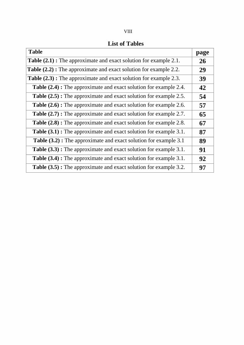
List of Tables
Table page
Table (2.1) : The approximate and exact solution for example 2.1. 26
Table (2.2) : The approximate and exact solution for example 2.2. 29
Table (2.3) : The approximate and exact solution for example 2.3. 39
Table (2.4) : The approximate and exact solution for example 2.4. 42
Table (2.5) : The approximate and exact solution for example 2.5. 54
Table (2.6) : The approximate and exact solution for example 2.6. 57
Table (2.7) : The approximate and exact solution for example 2.7. 65
Table (2.8) : The approximate and exact solution for example 2.8. 67
Table (3.1) : The approximate and exact solution for example 3.1. 87
Table (3.2) : The approximate and exact solution for example 3.1 89
Table (3.3) : The approximate and exact solution for example 3.1. 91
Table (3.4) : The approximate and exact solution for example 3.1. 92
Table (3.5) : The approximate and exact solution for example 3.2. 97

IX
List of Figures
Figures Page
Figure (1) : shows the approximate and the exact solution for example (2.1) that was
solved by shooting method.
27
Figure(2) : shows the approximate and the exact solution for example (2.2) that was
solved by shooting method.
30
Figure (3) : shows the approximate and the exact solution for example (2.3) that was
solved by shooting method.
40
Figure (4): shows the approximate and the exact solution for example (2.4) that was
solved by shooting method.
43
Figure (5): shows the approximate and the exact solution for example
(2.5) that was solved by finite difference method.
55
Figure (6) : shows the approximate and the exact solution for example (2.6) that was
solved by finite difference method.
58
Figure( 7): shows the approximate and the exact solution for example (2.7) that was
solved by finite difference method.
66
Figure( 8) : shows the approximate and the exact solution for example (2.8) that was
solved by finite difference method.
68
Figure(9): shows the approximate and the exact solution for example (3.1) that was
solved by finite difference method.
88
Figure(10): shows the approximate and the exact solution for example (3.1) that
was solved by shooting method.
90
Figure( 11): Emden problem – BVP with singular term.
96

X
Singular Two Points
Boundary Value Problem
By
Sawsan Mohammad Hamdan
Supervised by
Dr. Samir Matar
Abstract
A singular Two points boundary value problem occur frequently in
mathematical modeling of many practical problems. To solve singular two
points boundary value problem for certain ordinary differential equations
having singular coefficients. Many numerical method such as shooting
method, finite difference method and pade approximation methods, have
been studied and analysed.

Chapter one

2
Introduction
1.1 Introduction
Mathematics is the body of knowledge centered on such concepts as
quantity, structure, space, and change, and also the academic discipline that
studies them. Benjamin Pierce called it " the science that draws necessary
conclusions".
Other practitioners of mathematics maintain that mathematics is the science
of pattern, and that mathematicians seek out patterns whether found in
numbers, space, science, computers, imaginary abstractions, or elsewhere.
Mathematicians explore such concepts, aiming to formulate new conjectures
and establish their findings by rigorous deduction from appropriately chosen
axioms and definitions.
Though the use of abstraction and logical reasoning, mathematics evolved
from counting, calculation, measurement, and the systematic study of the
shapes and motions of physical objects. Knowledge and use of basic
mathematics have always been an inherent and integral part of individual
and group life. Refinements of the basic ideas are visible in mathematical
texts originating in the ancient Egyptian, Mesopotamian, Indian, Chinese,
Greek and Islamic worlds. Rigorous arguments first appeared in Greek
mathematics, most notably in Euclid's elements. The development continued
in fitful bursts until the renaissance period of the 16th century,
when mathematical innovations interacted with new scientific discoveries,
leading to an acceleration in research that continues to the present day.

3
Today, mathematics is used throughout the world in many fields, including
natural science, engineering, medicine, and the social sciences such as
economics.
Applied mathematics, the application of mathematics to such fields, inspires
and makes use of new mathematical discoveries and sometimes leads to the
development of entirely new disciplines. See [13]
1.2 Differential Equation
A differential equation is a mathematical equation for an unknown function
of one or several variables that relates the values of the function itself and of
its derivatives of various orders. Differential equations play a prominent role
in engineering, physics, economics and other disciplines.
Differential equations arise in many areas of science and technology,
whenever a deterministic relationship involving some continuously changing
quantities (modeled by functions) and their rates of change (expressed as
derivatives) is known or postulated. This is well illustrated by classical
mechanics, where the motion of a body is described by its position and
velocity as the time varies. Newton's laws allow one to relate the position,
velocity, acceleration and various forces acting on the body and state this
relation as a differential equation for the unknown position of the body as a
function of time. In many cases, this differential equation may be solved
explicitly, yielding the law of motion. See [3]&[13]
4
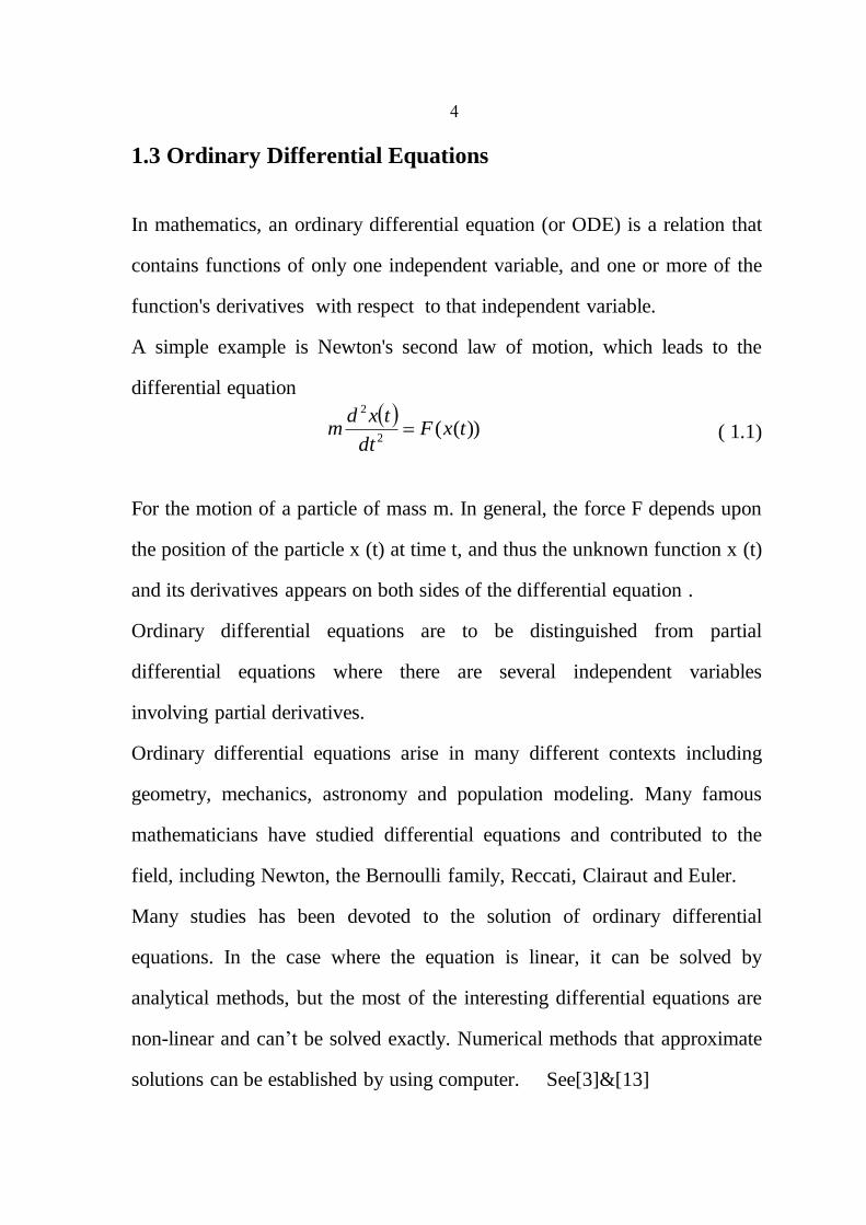
1.3 Ordinary Differential Equations
In mathematics, an ordinary differential equation (or ODE) is a relation that
contains functions of only one independent variable, and one or more of the
function's derivatives with respect to that independent variable.
A simple example is Newton's second law of motion, which leads to the
differential equation
))((
2
2
txFdt
txdm ( 1.1)
For the motion of a particle of mass m. In general, the force F depends upon
the position of the particle x (t) at time t, and thus the unknown function x (t)
and its derivatives appears on both sides of the differential equation .
Ordinary differential equations are to be distinguished from partial
differential equations where there are several independent variables
involving partial derivatives.
Ordinary differential equations arise in many different contexts including
geometry, mechanics, astronomy and population modeling. Many famous
mathematicians have studied differential equations and contributed to the
field, including Newton, the Bernoulli family, Reccati, Clairaut and Euler.
Many studies has been devoted to the solution of ordinary differential
equations. In the case where the equation is linear, it can be solved by
analytical methods, but the most of the interesting differential equations are
non-linear and can‟t be solved exactly. Numerical methods that approximate
solutions can be established by using computer. See[3]&[13]

5
1.4 Initial Value Problems
In mathematics, in the field of differential equations, an initial value problem
(IVP) is an ordinary differential equation together with specified values,
called the initial conditions, of the unknown function at a given point in the
domain of the solution. In physics or other sciences, modeling a system
frequently amounts to solving an initial value problem the differential
equation is an evolution equation specifying how, given initial conditions.
A simple form of initial value problem (IVP) is a differential equation
y' (t) = f ( t , y (t) ) (1.2)
with initial condition 00 )( yty .
A solution to an initial value problem is a function y that is a solution to the
differential equation and satisfies the initial condition 00 )( yty .
1.5 Boundary Value Problems
A boundary value problems (BVP) is a differential equation together with a
set of additional restrictions on the boundaries, called the boundary
conditions. A solution to the boundary value problem is a solution to the
differential equation which also satisfies the boundary conditions.
Boundary value problems arise in several branches of science. For example
in physical differential equation for some problems involving the wave
equation, such as the determination of normal modes, are often stated as
boundary value problems.
6
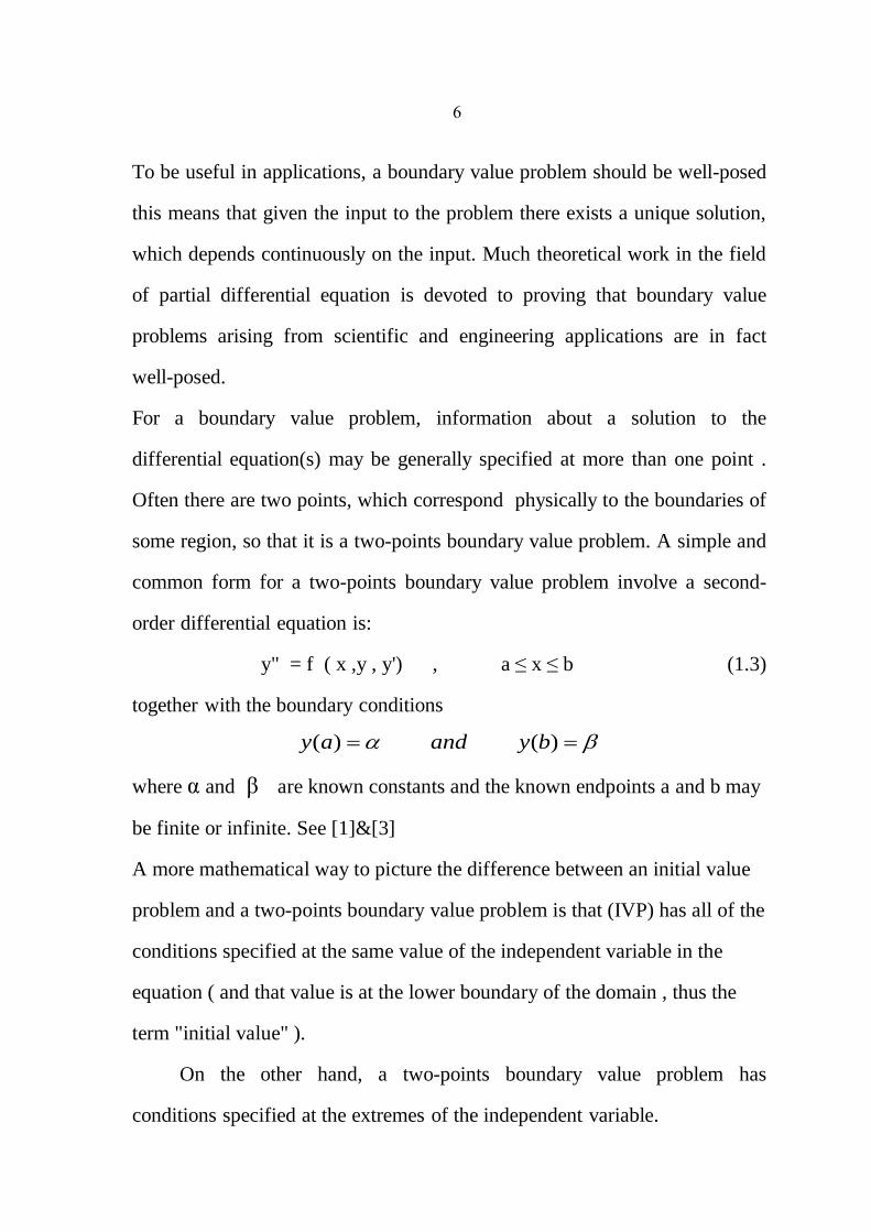
To be useful in applications, a boundary value problem should be well-posed
this means that given the input to the problem there exists a unique solution,
which depends continuously on the input. Much theoretical work in the field
of partial differential equation is devoted to proving that boundary value
problems arising from scientific and engineering applications are in fact
well-posed.
For a boundary value problem, information about a solution to the
differential equation(s) may be generally specified at more than one point .
Often there are two points, which correspond physically to the boundaries of
some region, so that it is a two-points boundary value problem. A simple and
common form for a two-points boundary value problem involve a second-
order differential equation is:
y" = f ( x ,y , y') , a ≤ x ≤ b (1.3)
together with the boundary conditions
)()( byanday
where α and β are known constants and the known endpoints a and b may
be finite or infinite. See [1]&[3]
A more mathematical way to picture the difference between an initial value
problem and a two-points boundary value problem is that (IVP) has all of the
conditions specified at the same value of the independent variable in the
equation ( and that value is at the lower boundary of the domain , thus the
term "initial value" ).
On the other hand, a two-points boundary value problem has
conditions specified at the extremes of the independent variable.
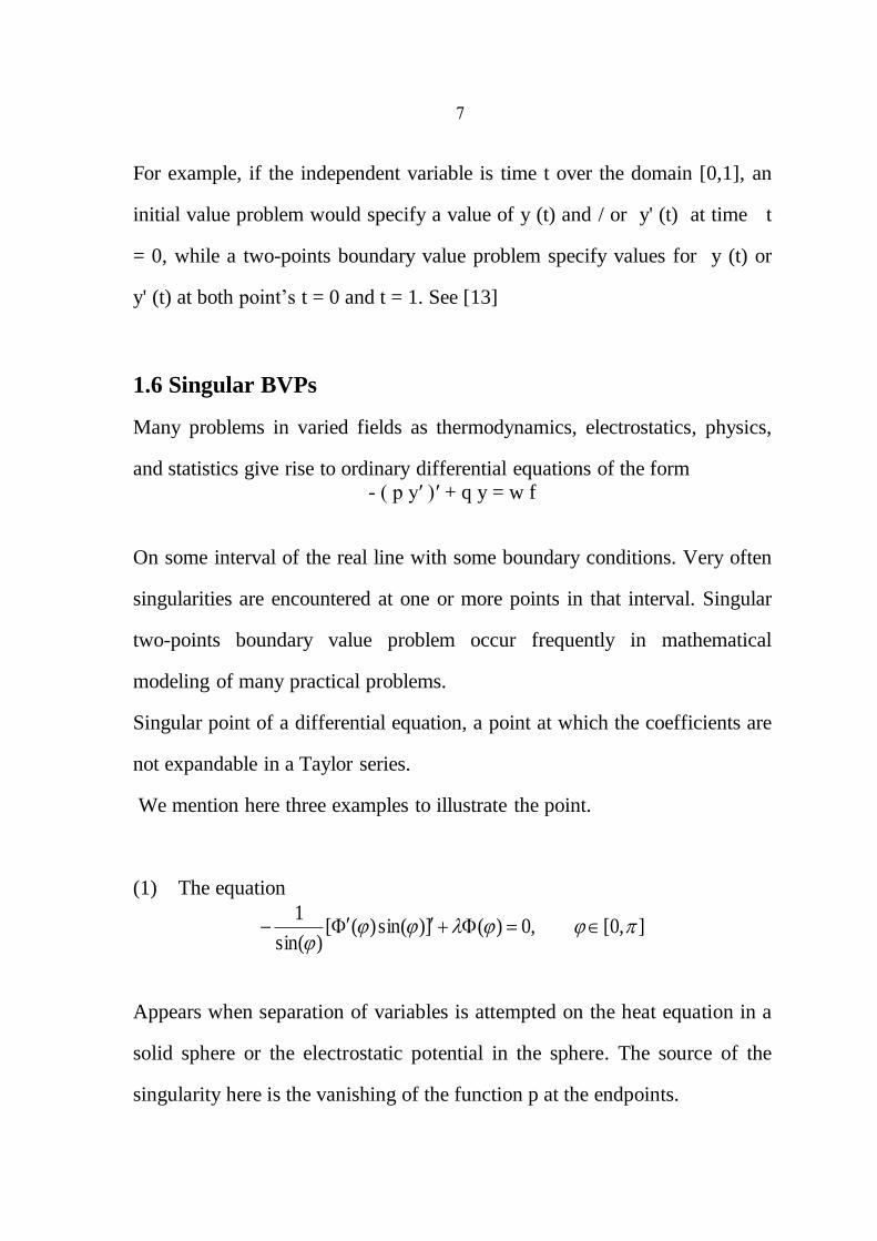
7
For example, if the independent variable is time t over the domain [0,1], an
initial value problem would specify a value of y (t) and / or y' (t) at time t
= 0, while a two-points boundary value problem specify values for y (t) or
y' (t) at both point‟s t = 0 and t = 1. See [13]
1.6 Singular BVPs
Many problems in varied fields as thermodynamics, electrostatics, physics,
and statistics give rise to ordinary differential equations of the form
- ( p y′ )′ + q y = w f
On some interval of the real line with some boundary conditions. Very often
singularities are encountered at one or more points in that interval. Singular
two-points boundary value problem occur frequently in mathematical
modeling of many practical problems.
Singular point of a differential equation, a point at which the coefficients are
not expandable in a Taylor series.
We mention here three examples to illustrate the point.
(1) The equation
],0[,0)(])sin()([)sin(
1
Appears when separation of variables is attempted on the heat equation in a
solid sphere or the electrostatic potential in the sphere. The source of the
singularity here is the vanishing of the function p at the endpoints.

8
(2) The equation
]1,1[),())1(( 2 xxfux
Represents the steady state temperature distribution in a bar extending from
-1 to 1 if the thermal conductivity is .The same type of
singularity occurs here also. See [5]
(3) An example of a class of singular BVP s is:
),()''( yxfyx (1.4)
0 < x ≤ 1 , y (0) = A , y (1) = B
In which 0 < α ≤ 1 and A , B are finite constants. We assume also that
for 0 < x < 1, the real-valued function f (x , y ) is continuous y
f
exists
and is continuous and that 0
y
f. See [10]
The obvious difficulty of the equation above is the behavior of the term
near x = 0.
1.7 Previous Works
Many previous works have been done on studied numerical methods for
solving singular BVPs, Gustafsson used some numerical methods that
treated only scalar problems, not systems, and does not deal at all with
existence or uniqueness of solutions. Natterer has treated systems, using a
projection method and has get )][ln( 2 rhhO accuracy. He also has dealt
)1( 2x
9
with existence and uniqueness of solutions, but has used unnatural looking
boundary conditions, and has not state when the problem will have a
solution, only when the operator is Fredholm with index zero (not when the
operator's inverse exists). Jamet also has treated only scalar equations and
has used three-point finite difference schemes, which, for a model problem,
with )( 1 hO accurate solutions )1,0(( is a parameter of the
problem). Shampine has dealt with a class of nonlinear second order scalar
equations, all with the same linear differential operator. He has proved
existence and uniqueness of solutions of this equation for certain boundary
value problems and the convergence of collocation and finite difference
methods. See [2]
[10] Twizell (1988) has developed numerical methods for this class of
BVPs (1.4). Twizell's methods gave more accurate numerical results than
those previously available (such as those of Chawla and Katti (1982) ). They
are also more economical and easier to implement. See [10]
In this thesis we have explored some numerical methods for solving singular
two-points boundary value problem and we have written some codes in
matlab.
This thesis contains three chapters. Chapter 2 contains the general forms for
the differential equation, and the type of boundary conditions, then we
discuss a numerical methods to solve BVP, Shooting method, and Finite
Difference method, for linear and nonlinear BVP.
01
Chapter 3 is devoted to singular two-points BVP. We discuss regular
singular point, singularities of the first kind, irregular singular point, infinite
interval problem, and other singular problem. Then some numerical methods
were used to solve singular two-points BVP.
In this work, some numerical methods for solving these problems have been
studied and analysed.
MATLAB is used as a computational tool during the development of this
thesis.

00
Chapter Two

02
Some Numerical methods for Solving Boundary Value
Problems
2.1 Introduction
A system of ordinary differential equations may have many solutions.
Commonly a solution of interest is determined by specifying the values of all
its components at a single point x = a. This point and a direction of
integration define an initial value problem (IVP).
In many applications the solution of interest is determined in a more
complicated way. A boundary value problem (BVP) specifies values or
equations for solution components at more than one point in the range of the
independent variable x. Generally IVP has a unique solution, but this is not
true for BVPs. Like a system of linear algebraic equations, a BVP may not
have a solution at all, or may have a unique solution, or may have more than
one solution. Because there might be more than one solution, BVP solvers
require an estimate (guess) for the solution of interest. Often there are
parameters that must be determined in order for the BVP to have a solution.
Associated with a solution there might be just one set of parameters, a finite
number of possible sets, or an infinite number of possible sets. See [9]

03
2.2 General Forms for the Differential Equations
For a second order non-linear BVPs we have the general form
y" (x) = f (x ,y (x) ,y' (x)) a ≤ x ≤ b
and the particular form that can be derived from the general one
y"(x) = f (x ,y (x)) a ≤ x ≤ b
These differential equations, valid in some interval [ a , b ], together with
(boundary) conditions imposed on the dependent variable and / or its first
derivative at the two points x = a and x = b give rise to the second order
general and special boundary value problems respectively.
For a linear boundary value problem which has the form
y" (x) = p (x) y' + q (x) y + r (x) a ≤ x ≤ b ,
with boundary conditions y (a) = α , y (b) = β
where p , q and r continuous functions on the interval [a , b].
Usually one assumes that a general ordinary differential equation can be
written as a first-order system
y ' = f ( x , y) a < x < b (2.1)
where (x)) y (x),..., y (x), (y (x) T
n21 y is the unknown vector function y
nR and T
n21 ))y ,(x f, , y) ,(x f , y) ,(x (f y) ,(x f is the (generally
nonlinear) right-hand side. The interval ends a and b are finite or infinite
constants. For a linear problem, the ODE simplifies to
y' =A (x) y + q (x) a < x < b (2.2)
04
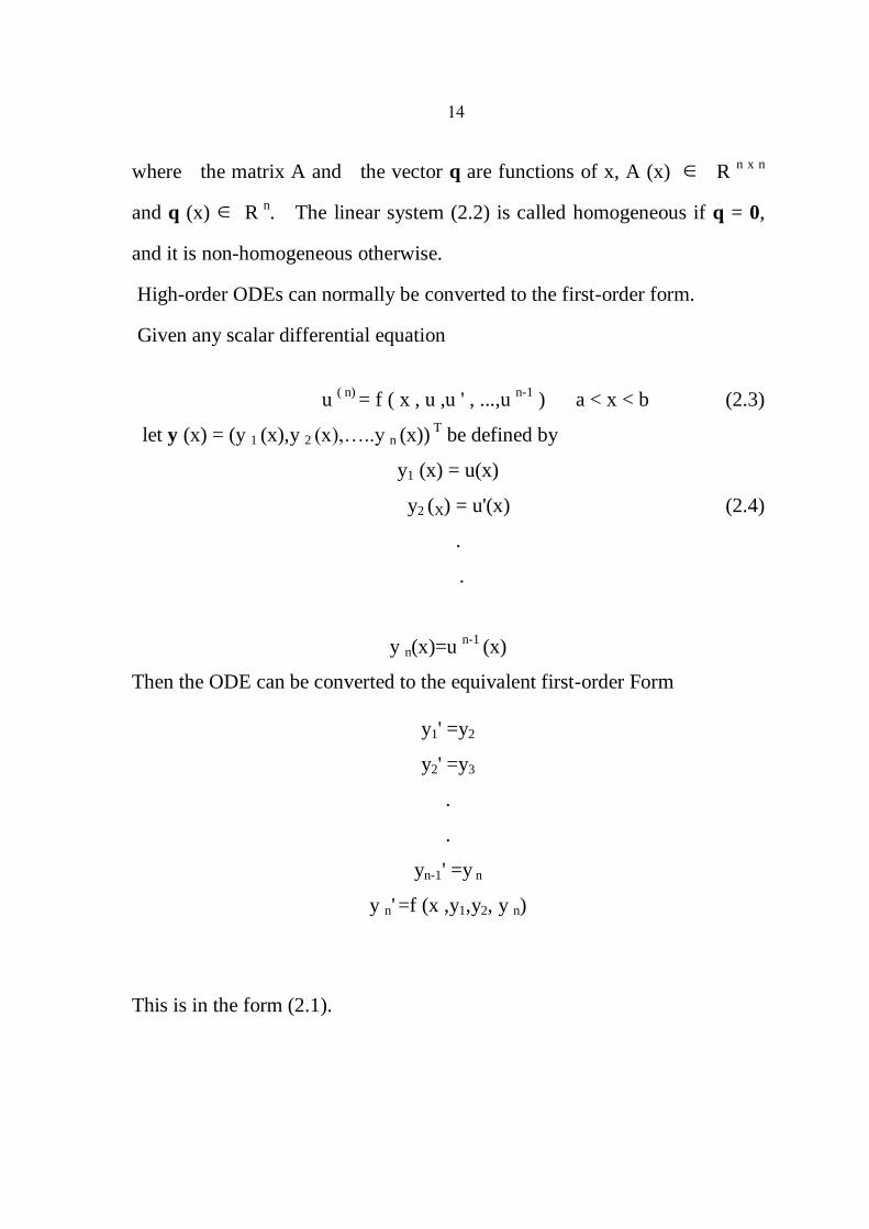
where the matrix A and the vector q are functions of x, A (x) R n x n
and q (x) R n
. The linear system (2.2) is called homogeneous if q = 0,
and it is non-homogeneous otherwise.
High-order ODEs can normally be converted to the first-order form.
Given any scalar differential equation
u ( n)
= f ( x , u ,u ' , ...,u n-1
) a < x < b (2.3)
let y (x) = (y 1 (x),y 2 (x),…..y n (x)) T
be defined by
y1 (x) = u(x)
y2 (X) = u'(x) (2.4)
.
.
y n(x)=u n-1
(x)
Then the ODE can be converted to the equivalent first-order Form
y1' =y2
y2' =y3
.
.
yn-1' =y n
y n' =f (x ,y1,y2, y n)
This is in the form (2.1).
05
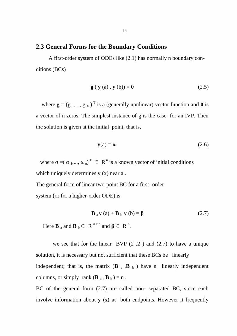
2.3 General Forms for the Boundary Conditions
A first-order system of ODEs like (2.1) has normally n boundary con-
ditions (BCs)
g ( y (a) , y (b)) = 0 (2.5)
where g = (g 1,..., g n ) T
is a (generally nonlinear) vector function and 0 is
a vector of n zeros. The simplest instance of g is the case for an IVP. Then
the solution is given at the initial point; that is,
y(a) = α (2.6)
where α =( α 1,..., α n) T
R n is a known vector of initial conditions
which uniquely determines y (x) near a .
The general form of linear two-point BC for a first- order
system (or for a higher-order ODE) is
B a y (a) + B b y (b) = β (2.7)
Here B a and B b R n x n
and β R n.
we see that for the linear BVP (2 .2 ) and (2.7) to have a unique
solution, it is necessary but not sufficient that these BCs be linearly
independent; that is, the matrix (B a ,B b ) have n linearly independent
columns, or simply rank (B a , B b ) = n .
BC of the general form (2.7) are called non- separated BC, since each
involve information about y (x) at both endpoints. However it frequently

06
happens that rank (B a) < n or rank (B b ) < n, or both. If either holds we call
the boundary condition partially separated.
In the case rank (B b) = q < n, the BVP can be transformed to one where the
BC have the form
Ba1y (a) = β 1
B a2 y (a) + B b2 y (b) = β 2 (2.8)
where B alR p X n
(p := n - q), B a2 and B b2R q X n
, β1 R p and β2R
q.
The BC are called separated if they simplify further to
Ba1 y (a) = β1
Bb2 y (b) = β2 (2.9)
The nonlinear BC (2.5) can also occur in partially separated or separated
form. Thus, the boundary conditions are separated if they are of the form
g 1 (y (a)) = 01
g 2 (y (b)) = 02 (2.10)
where g 1, 01 R p and g 2, 0 2 R
q with n = p + q.
In fact, a significant portion of the currently available software for BVPs
assumes that the BC are separated. See [1]
07
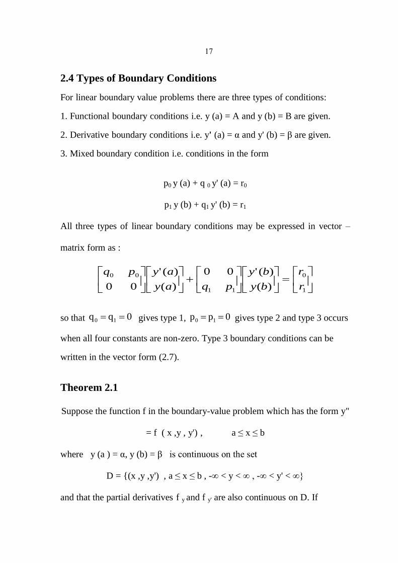
2.4 Types of Boundary Conditions
For linear boundary value problems there are three types of conditions:
1. Functional boundary conditions i.e. y (a) = A and y (b) = B are given.
2. Derivative boundary conditions i.e. y' (a) = α and y' (b) = β are given.
3. Mixed boundary condition i.e. conditions in the form
p0 y (a) + q 0 y' (a) = r0
p1 y (b) + q1 y' (b) = r1
All three types of linear boundary conditions may be expressed in vector –
matrix form as :
1
0
11
00
)(
)('00
)(
)('
00 r
r
by
by
pqay
aypq
so that 0 q q 10 gives type 1, 0 p p 10 gives type 2 and type 3 occurs
when all four constants are non-zero. Type 3 boundary conditions can be
written in the vector form (2.7).
Theorem 2.1
Suppose the function f in the boundary-value problem which has the form y"
= f ( x ,y , y') , a ≤ x ≤ b
where y (a ) = α, y (b) = β is continuous on the set
D = {(x ,y ,y') , a ≤ x ≤ b , -∞ < y < ∞ , -∞ < y' < ∞}
and that the partial derivatives f y and f y' are also continuous on D. If
08
(i) f y(x ,y ,y') > 0 For all (x ,y ,y') D and
(ii) a constant M exists with
| f y' ( x ,y ,y') | ≤ M for all ( x, y , y' ) D
Then the boundary-value problem has a unique solution. See[11]
* Note that theorem (2.1) gives the conditions under which the general BVP
with type 1 boundary condition has unique solution (existence and
uniqueness).
When f (x ,y ,y') has the form
f ( x ,y ,y') = p (x) y' + q (x) y + r (x)
the differential equation (1.3) is said to be linear.
Theorem (2.1) can be replaced by the following theorem:
Theorem 2.2
If the linear boundary value problem:
y" (x) = p (x) y' + q (x) y + r (x) (2.11)
a ≤ x ≤ b , y (a) = α , y (b) = β
satisfies:
(i) p (x), q (x) and r (x) are continuous on [a ,b]
(ii) q (x) > 0 on [a , b]
then (2.11) has a unique solution. See [11]

09
2.5 Linear Second-Order BVP s
Consider the linear second order BVP (2.11). let y o= y, y1= y' then (2.11)
can be written as the system of first order differential equations:
ry
y
pqy
y 010
'
'
1
0
1
0
Which can be written in vector-matrix form as:
D y = Q y + P (2.12)
With boundary conditions y0 (0) = A , y1 (1) = B. See [10]
Numerical Methods To Solve BVP.
2.6 Shooting Method:
The simplest initial value method for BVPs is the single shooting method,
it's one of the more successful numerical techniques for solving the general
BVP with type 1 boundary conditions based on the idea of reformulating the
problem as a sequence of IVPs of the form (1. 3) with y (a) = A
z (a) y' i , i = 0,1, …. (2.13)
To do this all conditions must be specified at one point. Suppose we choose
to impose some initial condition, at t = a, where there are some boundary
conditions are already known.
We guess the remaining boundary conditions at this point and, for the
moment, ignore the known boundary conditions at t = b. We now have an
IVP which can be solved using Range Kutta or any other appropriate
21
method to obtain a numerical solution at t = b. These numerical values are
then compared with the known boundary condition at t = b. If the guessed
initial conditions are correct, there will be no discrepancies with the known
boundary conditions at t = b, and the solution to the IVP will be the solution
to BVP. If not, we need to modify the guessed initial conditions at t = a.
This is called the shooting method, for obvious reasons. See [3]
It is probably clear to the reader that 'shooting methods' are so-called
because of the analogy of firing missiles at a stationary target. Starting with
the parameter 0z , which determines the initial elevation at which the missile
is discharged from the point (x , y ) = (a , A). The trajectory of the missile is
computed by solving the initial value problem given by (1.3) and (2.13) with
i > 0. If the point of landing, (x , y) = (b , y ( b, 0
z )) is not sufficiently close
to (b , B), the approximation is corrected by choosing another elevation 1z ,
and so on, until y(b , kz ) is acceptably close to the 'target' y (b) = B. See
[11]
Definition : A function f (t, y) is said to satisfy a Lipschitz condition in the
variable y on a set 2RD if a constant L > 0 exists with
2121 ),(),( yyLytfytf
Whenever Dytyt ),(),,( 21 . The constant L is called a Lipschitz constant
for f.
20
2.6.1 Shooting For Linear Problems
Consider the initial-value problems
bxaxryxqyxpy )()()( (2.14)
)(ay (2.15)
0)( ay (2.16)
And
bxayxqyxpy )()( (2.17)
0)( ay (2.18)
1)( ay (2.19)
If p, q, r continuous and q > 0 on [a,b] then the Lipschitz condition exists and
(2.14) to (2.19) have unique solutions.
Take )(1 xy solution of (2.14) to (2.16), and )(2 xy solution of (2.17) to
(2.19), and take
)()(
)()()( 2
2
11 xy
by
byxyxy
0)(2 by (2.20)
Where )(1 by is the approximated solution for (2.14) to (2.16) at x = b,
and )(2 by is the approximated solution for (2.17) to (2.19) at x = b.
Can be checked to be unique solution of BVP (2.11), and
)()(
)()()( 2
2
11 xy
by
byxyxy
(2.21)
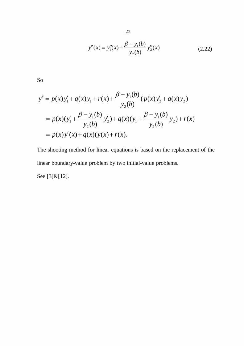
22
)()(
)()()( 2
2
11 xy
by
byxyxy
(2.22)
So
).()()(()()(
)())(
)()(()
)(
)()((
))()(()(
)()()()(
2
2
112
2
11
22
2
111
xrxyxqxyxp
xryby
byyxqy
by
byyxp
yxqyxpby
byxryxqyxpy
The shooting method for linear equations is based on the replacement of the
linear boundary-value problem by two initial-value problems.
See [3]&[12].

23
Algorithm 2.1
Linear shooting
To approximate the solution of the boundary-value problem
:)(,)(..0)()(')(" byaybxaxryxqyxpy
INPUT :endpoints a, b; boundary conditions , ; number of subintervals N.
OUTPUT : approximations iw ,1 to )( ixy ; iw ,2 to )(' ixy for each i =
0,1,…..,N.
Step 1 Set h = (b-a) / N:
.1
;0
;0
;
0,2
0,1
0,2
0,1
v
v
u
u
Step 2 For i = 0,…..,N-1 do steps 3 and 4.
(The Runge-Kutta method for systems is used in steps 3 and 4).
Step 3 Set x = a + ih.
Step 4 Set
];[
)];2/())(2/(
))(2/([
];[
)];()()([
;
2,221
,21,3
1,121
,1
2,121
,22,2
2,121
,21,2
,1,22,1
,21,1
kuhk
hxrkuhxq
kuhxphk
kuhk
xruxquxphk
huk
i
i
i
i
ii
i

24
].22[
];22[
)];)(())(([
];[
)];,)(2/())(2/([
];[
)];)(2/())(2/([
];[
];)()([
;
];22[
];22[
)];())(())(([
];[
)];2/())(2/(
))(2/([
2,42,32,22,161
,21,2
1,41,31,21,161
,11,1
1,3,12,3,22,4
2,3,21,4
1.221
,12,221
,22,3
2,221
,21,3
1,121
,12,121
,22,2
2,121
,21,2
,1,22,1
,21,1
2,42,32,22,161
,21,2
1,41,31,21,161
,11,1
1,3,12,3,22,4
2,3,21,4
1,221
,1
2,221
,22,3
kkkkvv
kkkkvv
kvhxqkvhxphk
kvhk
kvhxqkvhxphk
kvhk
kvhxqkvhxphk
kvhk
vxqvxphk
hvk
kkkkuu
kkkkuu
hxrkuhxqkuhxphk
kuhk
hxrkuhxq
kuhxphk
ii
ii
ii
i
ii
i
ii
i
ii
i
ii
ii
ii
i
i
i
Step 5 Set
N
N
v
uw
w
,1
,1
0,2
0,1 ;
;
OUTPUT ),,( 0,20,1 ww
Step 6 For i = 1, …. ,N
Set ;2
;1
,20,2,2
,10,2,1
ii
ii
vwuW
vwuW
x = a +ih;
OUTPUT (x,W1,W2), (Output is ii ww ,2,1 ,, .)
25
Step 7 STOP. (The process is complete.)See [3]
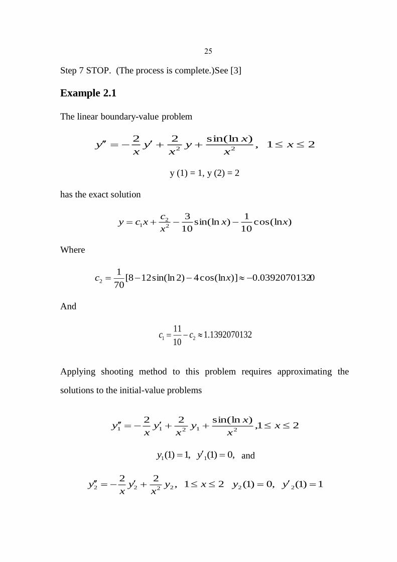
Example 2.1
The linear boundary-value problem
21,)sin(ln22
22 x
x
xy
xy
xy
y (1) = 1, y (2) = 2
has the exact solution
)cos(ln10
1)sin(ln
10
32
21 xx
x
cxcy
Where
00392070132.0)]cos(ln4)2sin(ln128[70
12 xc
And
1392070132.110
1121 cc
Applying shooting method to this problem requires approximating the
solutions to the initial-value problems
21,)sin(ln22
21211 xx
xy
xy
xy
,0)1(,1)1( 11 yy and
1)1(,0)1(21,22
222222 yyxyx
yx
y

26
Algorithm 2.1 uses the fourth-order Runge-Kutta technique to find the
approximation to y1(x) and y2(x).
The results of the calculations with N =10 and h = 0.1 are given in table
(2.1). The value listed as iw approximates and )( ixy is the exact solution
and iee is the error between the exact solution and the approximate solution.
)()2(
)2(2)()( 2
2
11 iii xy
y
yxyxy
. See [3] Program 1
Table (2.1) : The approximate and exact solution for example 2.1.
ix iw )( ixy
iii wxyee )(
1.000 1.000000 1.000000 0.000000
1.100 1.098134 1.092629 0.005505
1.200 1.194476 1.187084 0.007391
1.300 1.290881 1.283382 0.007498
1.400 1.388198 1.381445 0.006753
1.500 1.486792 1.481159 0.005633
1.600 1.586783 1.582392 0.004391
1.700 1.688171 1.685013 0.003157
1.800 1.790895 1.788898 0.001997
1.900 1.894870 1.893929 0.000941
2.000 2.000000 2.000000 0.000000
The maximum error is 0.007498.
27
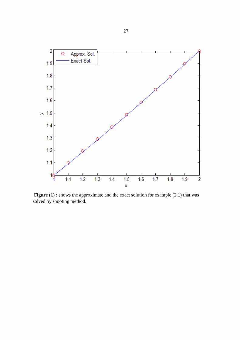
Figure (1) : shows the approximate and the exact solution for example (2.1) that was
solved by shooting method.

28
Example 2.2
The boundary-value problem
10),(4 xxyy , y (0) = 0, y (1) =1
has the exact solution
xeeeexy xx )()1()( 22142
Applying the shooting method to this problem requires approximating the
solutions to the initial-value problems
0)0(0)0(10),(4 1111 yyxxyy
0)0(0)0(10),(4 2222 yyxyy
Algorithm 2.1 uses the fourth-order Runge-Kutta technique to find the
approximation to y1(x) and y2(x), which can be found in page 22.
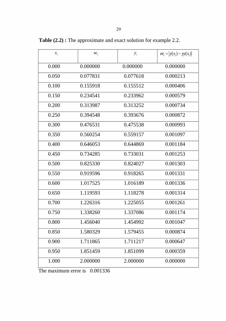
The results of the calculations with N = 20 and h =1/20 are given in table
(2.2). The value listed as iw approximates and )( ixy is the exact solution
and iee is the error between the exact solution and the approximate solution.
)()1(
)1(1)()( 2
2
11 iii xy
y
yxyxy
. See [3] program 2
29
Table (2.2) : The approximate and exact solution for example 2.2.
ix iw iy )()( iii xyyxyee
0.000 0.000000 0.000000 0.000000
0.050 0.077831 0.077618 0.000213
0.100 0.155918 0.155512 0.000406
0.150 0.234541 0.233962 0.000579
0.200 0.313987 0.313252 0.000734
0.250 0.394548 0.393676 0.000872
0.300 0.476531 0.475538 0.000993
0.350 0.560254 0.559157 0.001097
0.400 0.646053 0.644869 0.001184
0.450 0.734285 0.733031 0.001253
0.500 0.825330 0.824027 0.001303
0.550 0.919596 0.918265 0.001331
0.600 1.017525 1.016189 0.001336
0.650 1.119593 1.118278 0.001314
0.700 1.226316 1.225055 0.001261
0.750 1.338260 1.337086 0.001174
0.800 1.456040 1.454992 0.001047
0.850 1.580329 1.579455 0.000874
0.900 1.711865 1.711217 0.000647
0.950 1.851459 1.851099 0.000359
1.000 2.000000 2.000000 0.000000
The maximum error is 0.001336

31
Figure(2) : shows the approximate and the exact solution for example (2.2) that was
solved by shooting method.
30
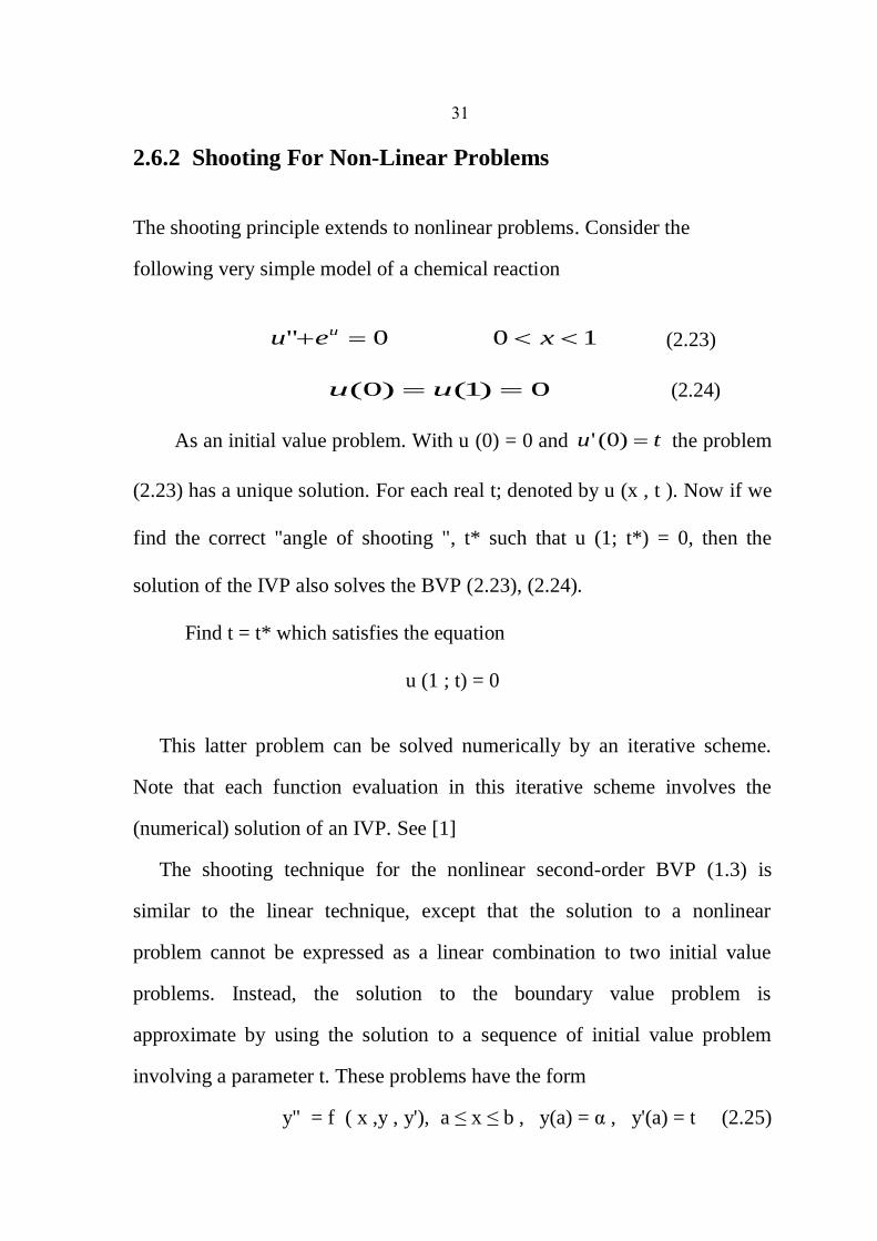
2.6.2 Shooting For Non-Linear Problems
The shooting principle extends to nonlinear problems. Consider the
following very simple model of a chemical reaction
100" xeu u (2.23)
0)1()0( uu (2.24)
As an initial value problem. With u (0) = 0 and tu )0(' the problem
(2.23) has a unique solution. For each real t; denoted by u (x , t ). Now if we
find the correct "angle of shooting ", t* such that u (1; t*) = 0, then the
solution of the IVP also solves the BVP (2.23), (2.24).
Find t = t* which satisfies the equation
u (1 ; t) = 0
This latter problem can be solved numerically by an iterative scheme.
Note that each function evaluation in this iterative scheme involves the
(numerical) solution of an IVP. See [1]
The shooting technique for the nonlinear second-order BVP (1.3) is
similar to the linear technique, except that the solution to a nonlinear
problem cannot be expressed as a linear combination to two initial value
problems. Instead, the solution to the boundary value problem is
approximate by using the solution to a sequence of initial value problem
involving a parameter t. These problems have the form
y" = f ( x ,y , y'), a ≤ x ≤ b , y(a) = α , y'(a) = t (2.25)
32
We do this by choosing the parameters t = tk in manner to ensure that
)(),(lim bytby kk
Where y(x, tk) denotes the solution to the initial value problem (2.25) with
t = tk and y (x) denotes the solution to the boundary value problem (1.3).
Start with a parameter t0 that determines the initial elevation at which the
object is fired from the point (a, α) and along the curve described by the
solution to the initial value problem:
y" = f ( x ,y , y'), a ≤ x ≤ b , y (a) = α , y' (a) = t0 .
If y (b, t0) is not sufficiently close to β, we correct our approximation
by choosing elevations t1, t2, and so on, until y(b, tk ) is sufficiently close to
β.
To determine the parameters tk, suppose a boundary value problem of
the form (1.3) satisfies theorem 2.1, 2.2 . If y(x, t) denotes the solution to the
initial value problem (2.25) we next determine t with
y (b, t) – β = 0 (2.26)
This is a nonlinear equation that can be solved by Newton's method
which use to generate the sequence { tk }, only one initial approximation, t0,
is needed.
The iteration has the form
33
),(
),(
1
11
k
kkk
tbdt
dy
tbytt
(2.27)
and it requires the knowledge of (dy/ dt) (b, tk-1). This presents a difficulty
since an explicit representation for y(b, t) is not known; we know only the
values y (b, t0), y (b, t1), …. , y (b, tk-1).
Suppose we rewrite the initial value problem (2.25), emphasizing that the
solution depends on both x and the parameter t:
y"(x, t) = f ( x ,y(x, t) , y'(x, t)),a ≤ x ≤ b , y (a, t) = α , y' (a, t) = t (2.28)
We have retained the prime notation to indicate differentiation with
respect to x. Since we need to determine (dy/ dt) (b, t) when t = tk-1, we first
take the partial derivative of (2.28) with respect to t. This implies that
).,('
)),('),,(,('
),()),('),,(,()),('),,(,(
)),('),,(,(),("
txt
ytxytxyx
y
f
txt
ytxytxyx
y
f
t
xtxytxyx
x
f
txytxyxt
ftx
dt
dy
Since x and t are independent, 0/ tx and
),('
)),('),,(,('
),()),('),,(,(),("
txt
ytxytxyx
y
ftx
t
ytxytxyx
y
ftx
t
y
(2.29)
For a ≤ x ≤ b. This initial conditions give
1),('
0),(
ta
t
yandta
t
y
34
If we simplify the notation by using z (x, t) to denote ),)(/( txty and
assume that the order of differentiation of x and t can be reversed, (2.29)
with the initial conditions becomes the initial value problem
),(')',,('
),()',,(),(" txzyyxy
ftxzyyx
y
ftxz
(2.30)
a ≤ x ≤ b, z (a, t) = 0, z (a, t) = 1
Newton's method therefore requires that two initial value problems be
solved for each iteration, (2.28) and (2.30). Then from (2.27),
),(
),(
1
11
k
kkk
tbz
tbytt
(2.31)
Of course, none of these initial value problems are solved exactly; the
solution are approximated. See [3] & [6]
Algorithm 2.2
Nonlinear Shooting with Newton’s Method
To approximate the solution of the nonlinear boundary-value problem
:)(,)(,).,,( byaybxayyxfy
INPUT : endpoints a, b; boundary conditions , ; number of subintervals N
≥ 2; tolerance TOL; maximum number of iterations M.

35
OUTPUT : approximations iw ,1 to ii wxy ,2);(to
)(' ixyfor each
i = 0,1, ……,N or a massage that the maximum number of iterations was
exceeded.
Step 1 Set h = (b-a) / N;
K = 1;
TK = ( - ) / (b - a). (note: TK could also be input.)
Step 2 While (k ≤ M) do steps 3-10.
Step 3 Set
.1
;0
;
2
1
0,2
0,1
u
u
TKw
w
Step 4 For i =1,…….,N do steps 5 and 6.
(The Runge-Kutta method for systems is used in steps 5and 6.)
Step 5 Set x = a +(i-1)h.
Step 6 Set

36

37
Step 7 If Nw ,1 ≤ TOL then do steps 8 and 9.
Step 8 For i = 0,1,……,N
set x = a + ih;
OUTPUT ),,( ,2,1 ii wwx .
Step 9 (The procedure is complete.)
STOP.
Step 10 Set 1
,1
u
wTKTK N
(Newton‟s method is used to compute TK.)
k = k+1.
Step 11 OUTPUT („Maximum number of iterations exceeded‟);
(The procedure was unsuccessful.)
STOP. See[3]
38
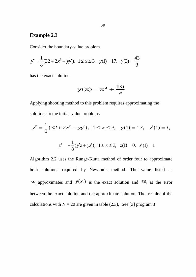
Example 2.3
Consider the boundary-value problem
3
43)3(,17)1(,31),232(
8
1 3 yyxyyxy
has the exact solution
x
16xy(x) 2
Applying shooting method to this problem requires approximating the
solutions to the initial-value problems
ktyyxyyxy )1(,17)1(,31),232(8
1 3
1)1(,0)1(,31),(8
1 zzxzyzyz
Algorithm 2.2 uses the Runge-Kutta method of order four to approximate
both solutions required by Newton‟s method. The value listed as
iw approximates and )( ixy is the exact solution and iee is the error
between the exact solution and the approximate solution. The results of the
calculations with N = 20 are given in table (2.3), See [3] program 3
39
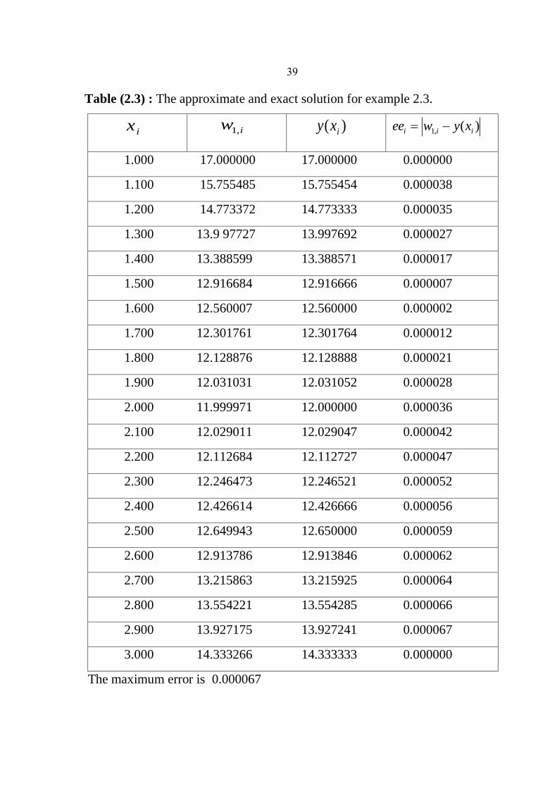
Table (2.3) : The approximate and exact solution for example 2.3.
ix iw ,1 )( ixy )(,1 iii xywee
1.000 17.000000 17.000000 0.000000
1.100 15.755485 15.755454 0.000038
1.200 14.773372 14.773333 0.000035
1.300 13.9 97727 13.997692 0.000027
1.400 13.388599 13.388571 0.000017
1.500 12.916684 12.916666 0.000007
1.600 12.560007 12.560000 0.000002
1.700 12.301761 12.301764 0.000012
1.800 12.128876 12.128888 0.000021
1.900 12.031031 12.031052 0.000028
2.000 11.999971 12.000000 0.000036
2.100 12.029011 12.029047 0.000042
2.200 12.112684 12.112727 0.000047
2.300 12.246473 12.246521 0.000052
2.400 12.426614 12.426666 0.000056
2.500 12.649943 12.650000 0.000059
2.600 12.913786 12.913846 0.000062
2.700 13.215863 13.215925 0.000064
2.800 13.554221 13.554285 0.000066
2.900 13.927175 13.927241 0.000067
3.000 14.333266 14.333333 0.000000
The maximum error is 0.000067
41
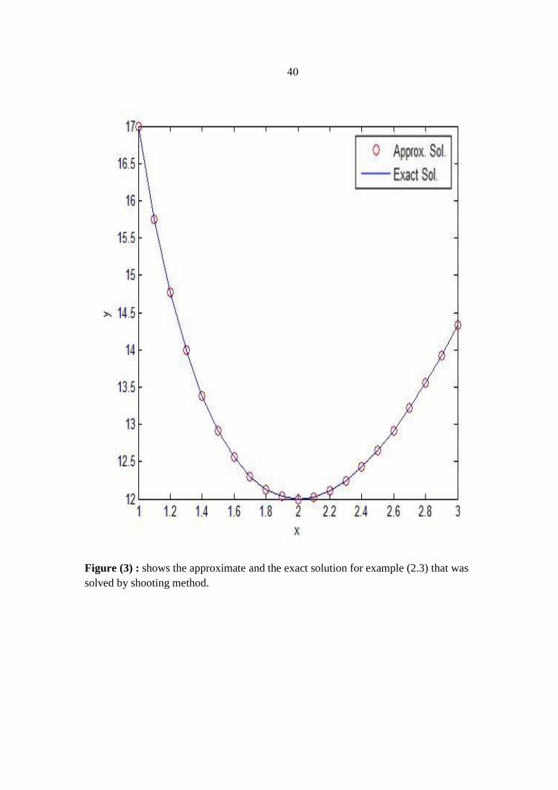
Figure (3) : shows the approximate and the exact solution for example (2.3) that was
solved by shooting method.

40
Example 2.4
Consider the non-linear boundary-value problem
3
1)2(,
2
1)1(,21,3 yyxyyyy
has the exact solution
1)1()( xxy
Applying shooting method to this problem requires approximating the
solutions to the initial-value problems
ktyyxyyyy )1(,2
1)1(,21,3
1)1(,0)1(,21),( zzxzyzyz
Algorithm 2.2 uses the Runge-Kutta method of order four to approximate
both solutions required by Newton‟s method (page 35). The value listed as
iw approximates and )( ixy is the exact solution and iee is the error
between the exact solution and the approximate solution. The results of the
calculations with N = 10 are given in table (2.4). See [3] program 3
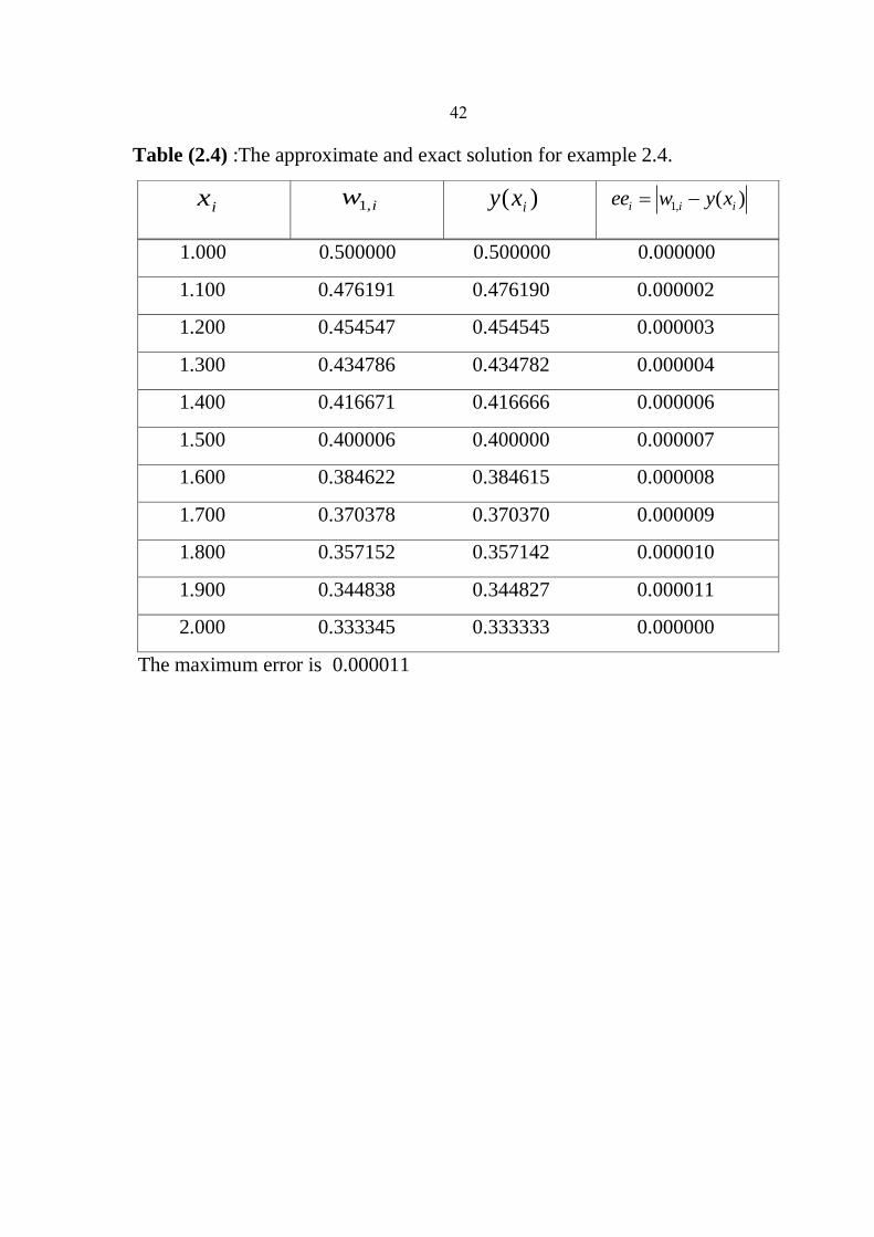
42
Table (2.4) :The approximate and exact solution for example 2.4.
1.000 0.500000 0.500000 0.000000
1.100 0.476191 0.476190 0.000002
1.200 0.454547 0.454545 0.000003
1.300 0.434786 0.434782 0.000004
1.400 0.416671 0.416666 0.000006
1.500 0.400006 0.400000 0.000007
1.600 0.384622 0.384615 0.000008
1.700 0.370378 0.370370 0.000009
1.800 0.357152 0.357142 0.000010
1.900 0.344838 0.344827 0.000011
2.000 0.333345 0.333333 0.000000
The maximum error is 0.000011
ix iw ,1 )( ixy )(,1 iii xywee

43
Figure (4): shows the approximate and the exact solution for example (2.4) that was
solved by shooting method.

44
2.7 Finite Difference Methods
In these methods, no initial value problems are explicitly integrated.
Rather, an approximate solution representation is sought over the entire
interval of interest. Thus, these methods are sometimes referred to as global
methods.
The basic steps of a finite difference method are outlined as follows,
we choose a mesh Ω to the interval [a,b], where
b)x ..xx(a 1N21 then approximate solution values are
then sought at these mesh points ix for i=2, 3, …, n
Form a set of algebraic equations for the approximate solution values by
replacing derivatives with difference quotients in the differential equations
and boundary conditions that the exact solution satisfies.
Finally, solve the resulting system of equations for the approximate solution,
this gives a set of discrete solution values )( ii xyy .
Finite difference methods proceed by replacing the derivatives in the
differential equations by finite difference approximations. This gives a large
algebraic system of equations to be solved in place of differential equation.
To approximate y' we can use one-sided approximation
h
xyhxyyxyD
)()(')(
or
h
hxyxyyxyD
)()(')(

45
Or we can use centered approximation :
h
hxyhxyyxyD
2
)()(')(0
Which is the average of the two one-sided approximations. It is clear that
Doy(x) gives a better approximation than either of the one-sided
approximations also it gives us a second order accurate approximation .
We can use finite difference to solve a differential equation consider the
second order differential equation
y"(x) = f (x), 0 < x < 1 (2.32)
y (0) = α y (1) = β
The function f (x) is specified and we wish to determine y (x) in the interval
0 < x < l. This problem is called two points boundary value problem. Since
boundary conditions are given at the two distinct points 0 and 1.
2.7.1 Simple One-Step Schemes for Linear first-order Systems
Consider now the linear first-order system
y' = A (x) y + f (x) , x [a , b] , y R n (2.33)
B a y (a) + B b y (b) = β (2.34)
and we seek numerical methods which work equally well for non-uniform
meshes. This naturally leads to one-step schemes, schemes which define the
difference operator based only on values related to one subinterval

46
1ii x,x of the mesh Ω at a time. The two simplest such finite difference
schemes are the midpoint and the trapezoidal schemes.
For a (generally non-uniform) mesh Ω, a discrete numerical solution
T
Nyyy ),......,,(y 121 is sought, Where yi is to approximate
component-wise the exact solution y(x) at ixx , i = 2, 3, …., N. The
numerical solution (in all methods based on one-step schemes) is required to
satisfy the boundary condition (2.34).
For the interior mesh points, two difference schemes are presented. For each
subinterval 1ii x,x i=1,2,3,…..,N-1,N, of Ω the derivative in (2.33) is
replaced by i
ii
h
yy 1
. This approximation is centered at
iii hxx2
1:2/1 , with )xx(:h i1ii at the middle of the subinterval.
Then A (x) y (x) + f (x) is approximated by a centered approximation,
yielding second-order accuracy. The trapezoidal scheme is defined by:
NixfxfyxAyxAh
yyiiiiii
i
ii
1)()(2
1)()(
2
1111
1(2.35)
and the midpoint scheme is defined by:
NixfyyxAh
yyiiii
i
ii
1)())((
2
12/112/1
1 (2.36)
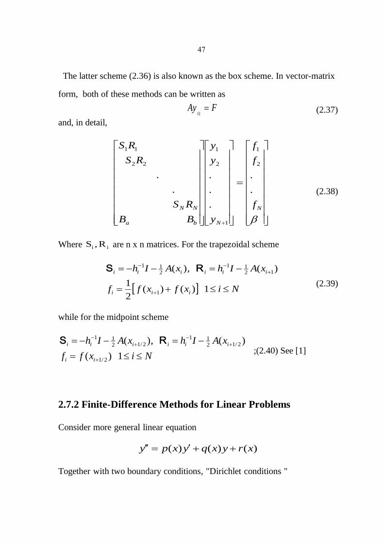
47
The latter scheme (2.36) is also known as the box scheme. In vector-matrix
form, both of these methods can be written as
FAy
(2.37)
and, in detail,
N
Nba
NN f
f
f
y
y
y
BB
RS
RS
RS
.
.
.
.
.
.
.
2
1
1
2
1
22
11
(2.38)
Where ii R,S are n x n matrices. For the trapezoidal scheme
Nixfxff
xAIhxAIh
iii
iiiiii
1)()(2
1
)(),(
1
1211
211 RS
(2.39)
while for the midpoint scheme
Nixff
xAIhxAIh
ii
iiiiii
1)(
)(),(
2/1
2/1211
2/1211 RS
;(2.40) See [1]
2.7.2 Finite-Difference Methods for Linear Problems
Consider more general linear equation
)()()( xryxqyxpy
Together with two boundary conditions, "Dirichlet conditions "

48
y (a) = α , y (b) = β
Let ,ihaxi i = 0, 1, 2, …, N+1 and ii xxh 1
This equation can be discretized to second order by:
iiiii
iiii ryq
h
yyp
h
yyy
2
)()2( 11
2
11, I = 1 ,2, …, N
Where, for example, )(),( iiii xqqxpp and )( ii xrr , this gives the
linear system A Y = F where A is the tri-diagonal matrix.
)2()2/1(
)2/1()2()2/1(
...
...
...
)2/1()2()2/1(
)2/1()2(
1
2
11
2
1
22
2
2
11
2
2
NN
NNN
qhhp
hpqhhp
hpqhhp
hpqh
hA
)2//1(
.
.
.
)2//1(
,
.
.
.
2
1
2
1
2
1
1
2
1
hphr
r
r
hphr
F
Y
Y
Y
Y
Yand
NN
N
N
N
This linear system can be solved with standard techniques assuming the
matrix is nonsingular. A singular matrix would be a sign that the discrete
system does not have a unique solution, which may occur if the original
problem, or nearby problem, is not well posed.

49
The discretization used above, while second order accurate, may not
be the best discretization to use for certain problems of this type. Often the
physical problem has certain properties that we would like to preserve with
our discretization, and it is important to understand the underlying problem
and be aware of its mathematical properties before blindly applying
numerical method. See [8]
2.7.3 Neumann Boundary Conditions
Consider we have one or more Neumann boundary conditions, instead
of Dirichlet boundary conditions, meaning that a boundary condition on the
derivative y' is given rather than a condition on the value of y itself. We
might have heat flux at a specified rate giving y' = α at this boundary.
Consider the equation (2.32) with boundary conditions:
y' (0) = α y (1) = β (2.41)
to solve this problem numerically, we need to introduce one more unknown
than we previously had: Yo at the point xo= 0 since this is now an unknown
value. We also need to augment the system (2.37) with one more equation
that models the boundary conditions (2.41). As a first try, we might use a
one-sided expression for y'(0) such as:
h
yy 01 (2.42)
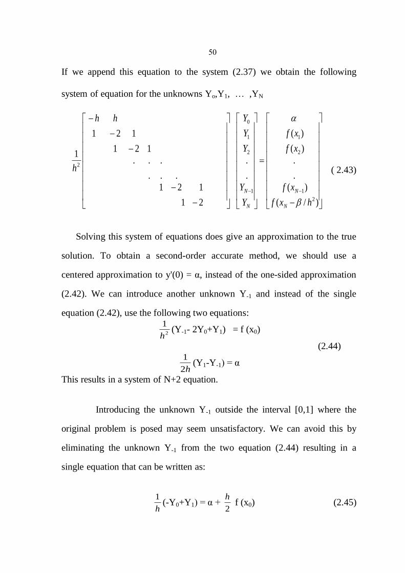
51
If we append this equation to the system (2.37) we obtain the following
system of equation for the unknowns Yo,Y1, … ,YN
)/(
)(
.
.
)(
)(
.
.
21
121
..
.
.
..
121
121
1
2
1
2
1
1
2
1
0
2
hxf
xf
xf
xf
Y
Y
Y
Y
Yhh
h
N
N
N
N
( 2.43)
Solving this system of equations does give an approximation to the true
solution. To obtain a second-order accurate method, we should use a
centered approximation to y'(0) = α, instead of the one-sided approximation
(2.42). We can introduce another unknown Y-1 and instead of the single
equation (2.42), use the following two equations:
2
1
h(Y-1- 2Y0+Y1) = f (x0)
(2.44)
h2
1(Y1-Y-1) = α
This results in a system of N+2 equation.
Introducing the unknown Y-1 outside the interval [0,1] where the
original problem is posed may seem unsatisfactory. We can avoid this by
eliminating the unknown Y-1 from the two equation (2.44) resulting in a
single equation that can be written as:
h
1(-Y0+Y1) = α +
2
h f (x0) (2.45)
50
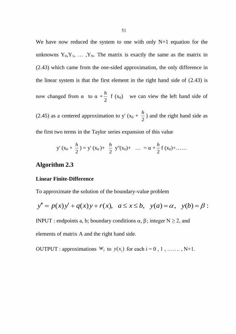
We have now reduced the system to one with only N+1 equation for the
unknowns Y0,Y1, … ,YN. The matrix is exactly the same as the matrix in
(2.43) which came from the one-sided approximation, the only difference in
the linear system is that the first element in the right hand side of (2.43) is
now changed from α to α +2
h f (x0) we can view the left hand side of
(2.45) as a centered approximation to y' (x0 + 2
h) and the right hand side as
the first two terms in the Taylor series expansion of this value
y' (x0 + 2
h) = y' (x0 )+
2
h y''(x0)+ … = α +
2
hf (x0)+……
Algorithm 2.3
Linear Finite-Difference
To approximate the solution of the boundary-value problem
:)(,)(,),()()( byaybxaxryxqyxpy
INPUT : endpoints a, b; boundary conditions , ; integer N ≥ 2, and
elements of matrix A and the right hand side.
OUTPUT : approximations iw to )( ixy for each i = 0 , 1 , ……. , N+1.
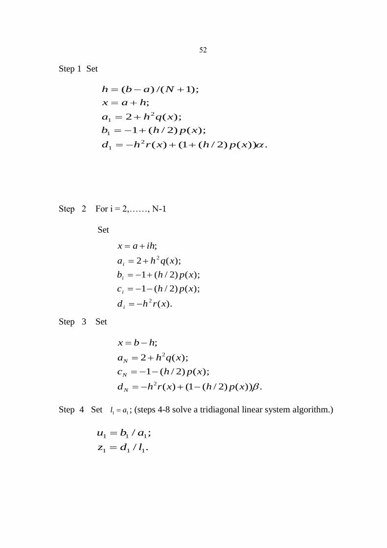
52
Step 1 Set
.))()2/(1()(
);()2/(1
);(2
;
);1/()(
2
1
1
2
1
xphxrhd
xphb
xqha
hax
Nabh
Step 2 For i = 2,……, N-1
Set
).(
);()2/(1
);()2/(1
);(2
;
2
2
xrhd
xphc
xphb
xqha
ihax
i
i
i
i
Step 3 Set
.))()2/(1()(
);()2/(1
);(2
;
2
2
xphxrhd
xphc
xqha
hbx
N
N
N
Step 4 Set 11 al ; (steps 4-8 solve a tridiagonal linear system algorithm.)
./
;/
111
111
ldz
abu
53
Step 5 For i = 2,……,N-1 set
iiiii
iii
iiii
lzcdz
lbu
ucal
/)(
/
1
1
Step 6 Set
./)(
;
1
1
NNNNN
NNNN
lzcdz
ucal
Step 7 Set
.
;
;
1
0
NN
N
zw
w
w
Step 8 For i = N-1, …… ,1 set .1 iiii wuzw
Step 9 For i = 0, ……. , N + 1 set x = a + ih;
OUTPUT ),( iwx .
Step 10 STOP. (The procedure is complete.)

54
Example 2.5
Algorithm (2.3) will be used to approximate the solution to the boundary-
value problem
21,)sin(ln22
22 x
x
xy
xy
xy
y (1) = 1, y (2) = 2
with h = 0.1 which was also approximated by the shooting method in
example (2.1), gives the results listed in table (2.5). The value listed as
iw approximates and )( ixy is the exact solution and iee is the error
between the exact solution and the approximate solution. program 4
Table(2.5) : The approximate and exact solution for example 2.5.
ix iw iy )()( iii xyxwee
The maximum error is 0.000045
1.000 1.000000 1.000000 0.000000
1.100 1.092600 1.092629 0.000028
1.200 1.187043 1.187084 0.000041
1.300 1.283336 1.283382 0.000045
1.400 1.381402 1.381445 0.000043
1.500 1.481120 1.481159 0.000039
1.600 1.582359 1.582392 0.000032
1.700 1.684989 1.685013 0.000024
1.800 1.788881 1.788898 0.000016
1.900 1.893921 1.893929 0.000008
2.000 2.000000 2.000000 0.000000
55
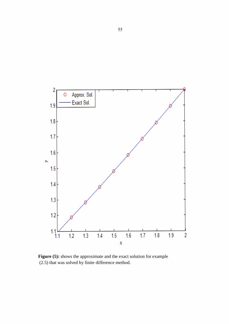
Figure (5): shows the approximate and the exact solution for example
(2.5) that was solved by finite difference method.

56
Example 2.6
Algorithm (2.3) will be used to approximate the solution to the boundary-
value problem
10),(4 xxyy , y (0) = 0, y (1) =1
with h = 1/20, which was also approximated by the shooting method in
example (2.2), gives the results listed in table (2.6). The value listed as
iw approximates and )( ixy is the exact solution and iee is the error
between the exact solution and the approximate solution. program 5
57
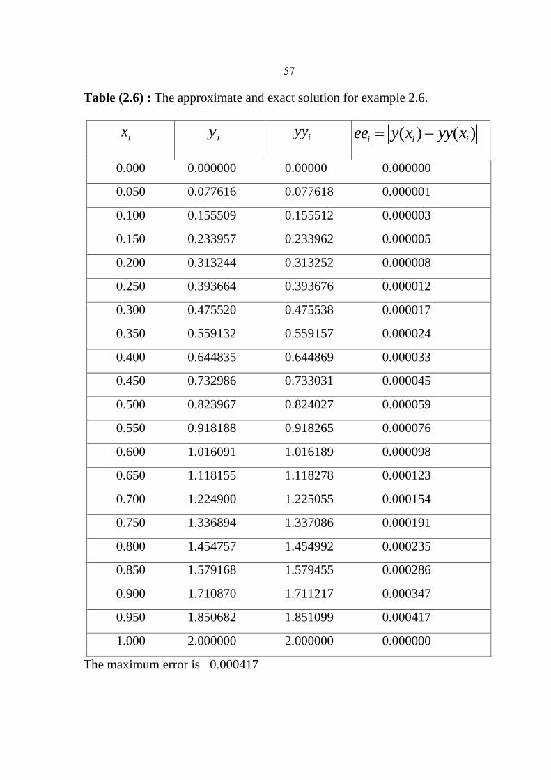
Table (2.6) : The approximate and exact solution for example 2.6.
ix iy iyy )()( iii xyyxyee
0.000 0.000000 0.00000 0.000000
0.050 0.077616 0.077618 0.000001
0.100 0.155509 0.155512 0.000003
0.150 0.233957 0.233962 0.000005
0.200 0.313244 0.313252 0.000008
0.250 0.393664 0.393676 0.000012
0.300 0.475520 0.475538 0.000017
0.350 0.559132 0.559157 0.000024
0.400 0.644835 0.644869 0.000033
0.450 0.732986 0.733031 0.000045
0.500 0.823967 0.824027 0.000059
0.550 0.918188 0.918265 0.000076
0.600 1.016091 1.016189 0.000098
0.650 1.118155 1.118278 0.000123
0.700 1.224900 1.225055 0.000154
0.750 1.336894 1.337086 0.000191
0.800 1.454757 1.454992 0.000235
0.850 1.579168 1.579455 0.000286
0.900 1.710870 1.711217 0.000347
0.950 1.850682 1.851099 0.000417
1.000 2.000000 2.000000 0.000000
The maximum error is 0.000417

58
Figure (6) : shows the approximate and the exact solution for example (2.6) that was
solved by finite difference method.
59
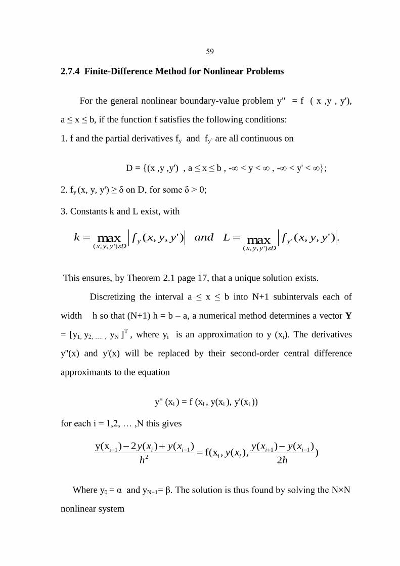
2.7.4 Finite-Difference Method for Nonlinear Problems
For the general nonlinear boundary-value problem y" = f ( x ,y , y'),
a ≤ x ≤ b, if the function f satisfies the following conditions:
1. f and the partial derivatives fy and fy‟ are all continuous on
D = {(x ,y ,y') , a ≤ x ≤ b , -∞ < y < ∞ , -∞ < y' < ∞};
2. fy (x, y, y') ≥ δ on D, for some δ > 0;
3. Constants k and L exist, with
.)',,()',,( '
)',,()',,(maxmax yyxfLandyyxfk y
Dyyx
yDyyx
This ensures, by Theorem 2.1 page 17, that a unique solution exists.
Discretizing the interval a ≤ x ≤ b into N+1 subintervals each of
width h so that (N+1) h = b – a, a numerical method determines a vector Y
= [y1, y2, …. , yN ]T
, where yi is an approximation to y (xi). The derivatives
y''(x) and y'(x) will be replaced by their second-order central difference
approximants to the equation
y'' (xi ) = f (xi , y(xi ), y'(xi ))
for each i = 1,2, … ,N this gives
)2
)()(),(,f(x
)()(2)y(x 11i2
11i
h
xyxyxy
h
xyxy iii
ii
Where y0 = α and yN+1= β. The solution is thus found by solving the N×N
nonlinear system
61
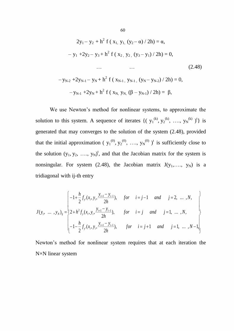
2y1 – y2 + h2
f ( x1, y1, (y2 – α) / 2h) = α,
– y1 +2y2 – y3 + h2
f ( x2 , y2 , (y3 – y1) / 2h) = 0,
… … (2.48)
– yN-2 +2yN-1 – yN + h2
f ( xN-1 , yN-1 , (yN – yN-2) / 2h) = 0,
– yN-1 +2yN + h2
f ( xN, yN, (β – yN-1) / 2h) = β,
We use Newton‟s method for nonlinear systems, to approximate the
solution to this system. A sequence of iterates {( y1(k)
, y2
(k), …., yN
(k) )
t} is
generated that may converges to the solution of the system (2.48), provided
that the initial approximation ( y1(0)
, y2
(0), …., yN
(0) )
t is sufficiently close to
the solution (y1, y2, …., yN)
t, and that the Jacobian matrix for the system is
nonsingular. For system (2.48), the Jacobian matrix J(y1,…., yN) is a
tridiagonal with ij-th entry
,1,...,11),2
,,(2
1
,,...,1),2
,,(2
,,...,21),2
,,(2
1
),...,(
11'
112
11'
1
Njandjiforh
yyyxf
h
Njandjiforh
yyyxfh
Njandjiforh
yyyxf
h
yyJ
iiiiy
iiiiy
iiiiy
ijN
Newton‟s method for nonlinear system requires that at each iteration the
N×N linear system

60
J(y1, …., yN) (v1,
…., vN)
t =
tNNNNN
NNNNNNN
h
yyxfhyy
h
yyyxfhyyy
h
yyyxfhyyy
h
yyxfhyy
))2
,,(2
),2
,,(2
),...,2
,,(2
),2
,,(2(
12
1
211
2
12
1322
2
321
211
2
21
Be solved for v1, v2 …., vN, since yi
(k) = yi
(k-1) + vi, for each i = 1, 2, … ,N.
See [3] & [10]
Algorithm 2.4
Nonlinear Finite-Difference
To approximate the solution to the nonlinear boundary-value problem
:)(,)(,).,,( byaybxayyxfy
INPUT : endpoints a, b; boundary conditions , ; integer N ≥ 2, tolerance
TOL; maximum number of iterations M.
OUTPUT : approximations iw to )( ixy for each i = 0,1,……,N+1 or a
message that the maximum number of iterations was exceeded.
Step 1 Set
.
;
);1/()(
1
0
Nw
w
Nabh
Step 2 For i = 1 ,……, N set .)( hab
iwi

62
Step 3 Set k = 1.
Step 4 While K ≤ M do steps 5-16.
Step 5 Set
)).,,(2(
);,,()2/(1
);,,(2
);2/()(
;
1
2
211
11
1
2
1
2
twxfhwwd
twxfhb
twxfha
hwt
hax
y
y
Step 6 For i = 2,……, N-1
set
)).,,(2(
);,,()2/(1
);,,()2/(1
);,,(2
);2/()(
;
2
11
2
11
twxfhwwwd
twxfhc
twxfhb
twxfha
hwwt
ihax
iiiii
iyi
iyi
iyi
ii
Step 7 Set
)).,,(2(
);,,()2/(1
);,,(2
);2/()(
;
2
1
2
1
twxfhwwd
twxfhc
twxfha
hwt
hbx
NNNN
NyN
NyN
N
Step 8 Set 11 al ; (steps 8-12 solve a tridiagonal linear system.)
./
;/
111
111
ldz
abu
63
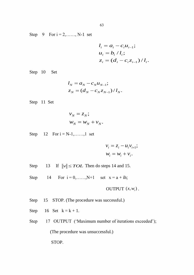
Step 9 For i = 2,……, N-1 set
./)(
;/
;
1
1
iiiii
iii
iiii
lzcdz
lbu
ucal
Step 10 Set
./)(
;
1
1
NNNNN
NNNN
lzcdz
ucal
Step 11 Set
.
;
NNN
NN
vww
zv
Step 12 For i = N-1,……,1 set
.
;1
iii
iiii
vww
vuzv
Step 13 If TOLv Then do steps 14 and 15.
Step 14 For i = 0,……,N+1 set x = a + ih;
OUTPUT ),( iwx .
Step 15 STOP. (The procedure was successful.)
Step 16 Set k = k + 1.
Step 17 OUTPUT („Maximum number of iterations exceeded‟);
(The procedure was unsuccessful.)
STOP.
64
Example 2.7
Consider the boundary-value problem
3
43)3(,17)1(,31),232(
8
1 3 yyxyyxy
has the exact solution
x
16xy(x) 2
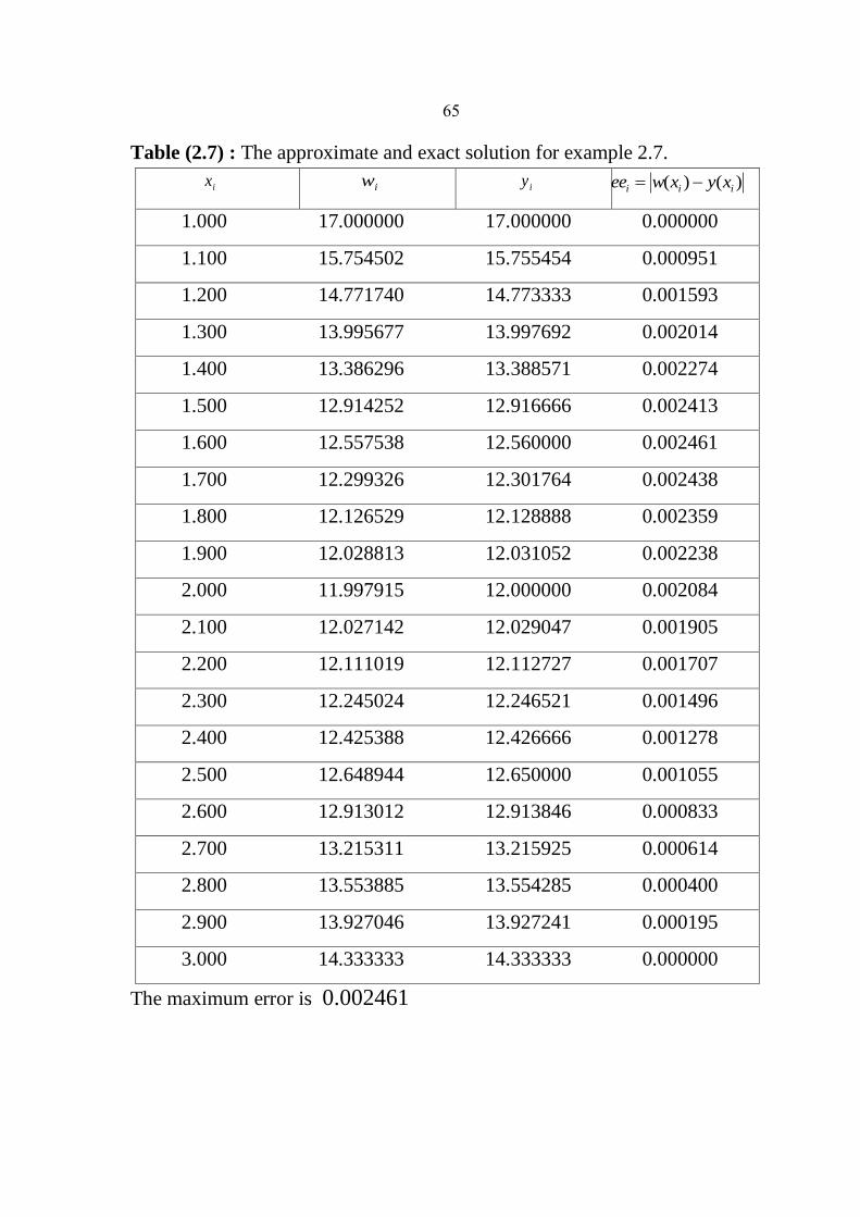
Applying finite difference method to this problem the solutions results in
table (2.7). The value listed as iw approximates and )( ixy is the exact
solution and iee is the error between the exact solution and the approximate
solution. program 6
65
Table (2.7) : The approximate and exact solution for example 2.7.
ix iw iy )()( iii xyxwee
1.000 17.000000 17.000000 0.000000
1.100 15.754502 15.755454 0.000951
1.200 14.771740 14.773333 0.001593
1.300 13.995677 13.997692 0.002014
1.400 13.386296 13.388571 0.002274
1.500 12.914252 12.916666 0.002413
1.600 12.557538 12.560000 0.002461
1.700 12.299326 12.301764 0.002438
1.800 12.126529 12.128888 0.002359
1.900 12.028813 12.031052 0.002238
2.000 11.997915 12.000000 0.002084
2.100 12.027142 12.029047 0.001905
2.200 12.111019 12.112727 0.001707
2.300 12.245024 12.246521 0.001496
2.400 12.425388 12.426666 0.001278
2.500 12.648944 12.650000 0.001055
2.600 12.913012 12.913846 0.000833
2.700 13.215311 13.215925 0.000614
2.800 13.553885 13.554285 0.000400
2.900 13.927046 13.927241 0.000195
3.000 14.333333 14.333333 0.000000
The maximum error is 0.002461

66
Figure( 7): shows the approximate and the exact solution for example (2.7) that was
solved by finite difference method.
67
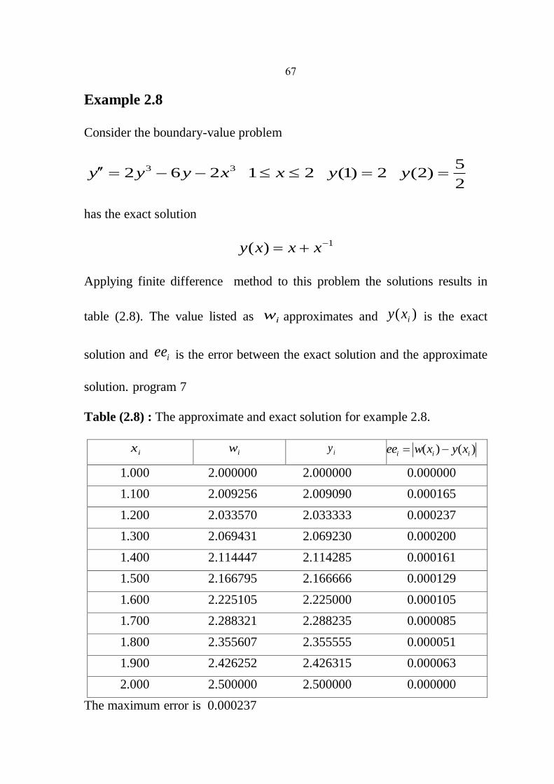
Example 2.8
Consider the boundary-value problem
2
5)2(2)1(21262 33 yyxxyyy
has the exact solution
1)( xxxy
Applying finite difference method to this problem the solutions results in
table (2.8). The value listed as iw approximates and )( ixy is the exact
solution and iee is the error between the exact solution and the approximate
solution. program 7
Table (2.8) : The approximate and exact solution for example 2.8.
ix iw iy )()( iii xyxwee
1.000 2.000000 2.000000 0.000000
1.100 2.009256 2.009090 0.000165
1.200 2.033570 2.033333 0.000237
1.300 2.069431 2.069230 0.000200
1.400 2.114447 2.114285 0.000161
1.500 2.166795 2.166666 0.000129
1.600 2.225105 2.225000 0.000105
1.700 2.288321 2.288235 0.000085
1.800 2.355607 2.355555 0.000051
1.900 2.426252 2.426315 0.000063
2.000 2.500000 2.500000 0.000000
The maximum error is 0.000237

68
Figure( 8) : shows the approximate and the exact solution for example (2.8) that was
solved by finite difference method.

69
Chapter Three

71
Singular Two-Points BVP
3.1 Introduction
Singular two-points boundary value problem occur frequently in
mathematical modeling of many practical problems.
We consider first a system of linear ordinary differential equations on a
finite interval with a singularity of the first kind at one endpoint. We treat the
same problem with singularities at both endpoints and with a singularity on
the interior of the interval.
Consider a class of singular BVPs:
ByAyxyxfyx )1(,)0(,10),,()''( (3.1)
In which 10 and A , B are finite constants, we assume also that for
0 < x < 1, the real-valued function f (x , y) is continuous, dy
dfexists and is
continuous and that dy
df > 0. See [2]
3.2 Regular Singular Point ,Singularities of The First Kind
Consider the ODE
-)'( yx f (x, y) = 0 0 < x < 1 (3.2)
If we assume here that α = 1 in (3.2). The assumptions on the regularity of a
solution y (x) of (3.2) imply that lim y (x) exists, as x decreases to 0.

70
This is needed in order to make the BVP for (3.2) meaningful, and is
reasonable in most applications. These assumptions further yield that
f (0 , y (0)) = 0 (3.3)
which must be compatible with the prescribed BC. In fact, the requirement
(3.3) is often used to determine part of the BC.
To be more specific, let us consider now the linear BVP which has a singular
point of the first kind
y' = A (x) y + q (x) 0 < x < 1 (3.4)
where )(~1
)( xx
x ARA (3.5)
here y (x), q (x), are n component vec n x n
matrices. R is a constant matrix, and q (x) C (0,1].
For any solution y (x) of (3.4), we require y (x) C¹(0,1] , we also impose a
linear system of two-points boundary conditions written as
)1()(lim 100
yBxyBx
(3.6)
note that we cannot merely write
y(1)B y(0)B 10 (3.7)
because y (x) is not even necessarily defined at x = 0. Notice also (3.7)
implies that )(lim 00
xyBx
is bounded.

72
Let the fundamental solution matrix, Y (x), for the homogeneous equation
for (3.4). That is, Y (x) satisfies
Y' = A (x) Y, x (0,1], Y ( 0x ) = I, 0x (0,1] (3.8)
Then every solution to (3.4) can be written
]1,0()( (x)cy(x) xxyY P (3.9)
where y (x) is any particular solution of (3.4) and where c is a constant
vector. where the particular solution py (x) satisfies
0)(,10)( pp yxxy (3.10)
Where 0 < δ < 1, See [2] & [7]
The smoothness of f (x, y) in (3.2) [or of A (X) and q (x) in (3.4)] does
not imply corresponding smoothness of y(x) near x = 0.
For example, the IVP
0 y(0) y, xy'21
has the solution x (x)y , which has an unbounded first derivative at
x = 0. However, where often the solution y (x) is nonetheless smooth near
the singularity. The performance of numerical methods for problems with
singularities of the first kind where the solution is smooth at the singularities.
73
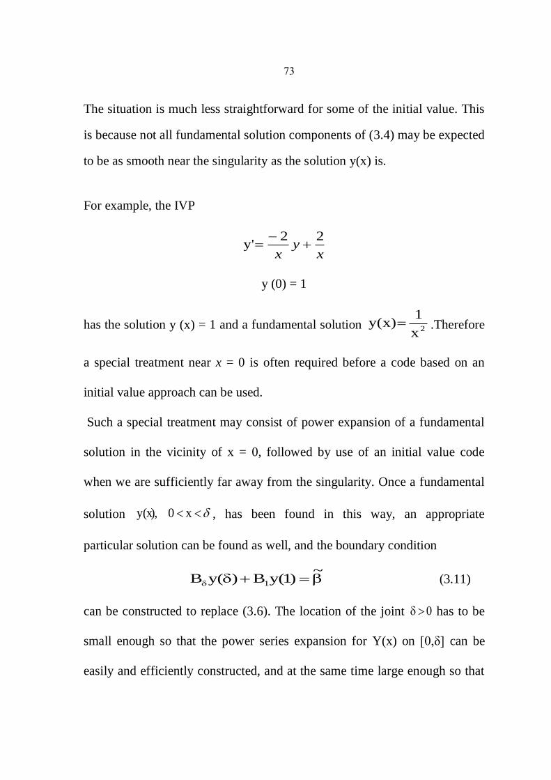
The situation is much less straightforward for some of the initial value. This
is because not all fundamental solution components of (3.4) may be expected
to be as smooth near the singularity as the solution y(x) is.
For example, the IVP
xy
x
22y'
y (0) = 1
has the solution y (x) = 1 and a fundamental solution 2x
1 y(x) .Therefore
a special treatment near x = 0 is often required before a code based on an
initial value approach can be used.
Such a special treatment may consist of power expansion of a fundamental
solution in the vicinity of x = 0, followed by use of an initial value code
when we are sufficiently far away from the singularity. Once a fundamental
solution x 0 y(x), , has been found in this way, an appropriate
particular solution can be found as well, and the boundary condition
~)1(yB)(yB 1 (3.11)
can be constructed to replace (3.6). The location of the joint 0 has to be
small enough so that the power series expansion for Y(x) on [0,δ] can be
easily and efficiently constructed, and at the same time large enough so that

74
the BVP (3.4), (3.11) on ,1][ can be solved by a standard initial value
method without difficulty. See [1]
3.3 Irregular Singular Point
There is at present no theoretical work justifying numerical methods for
solving problems with irregular singular points. The main practical
occurrence of such problems seems to be those formulated on infinite
intervals and we examine some simple examples here. See [7]
Suppose that we have the ODE
0(x)y)(x, ' ayAfy (3.12)
Then a transformation
t = x
a (3.13)
reformulates (3.12) as an ODE defined on the interval (0,1], namely
),(2 yt
aaf
dt
dyt (3.14)
in which we recognize an ODE with a singularity of the second kind. In
(3.13) we have assumed that a > 0. If a ≤ 0 then the transformation
axt
1
1 and reformulates (3.12) as an ODE defined on the interval
(0,1], namely.
),11
(2 yat
fdt
dyt
75
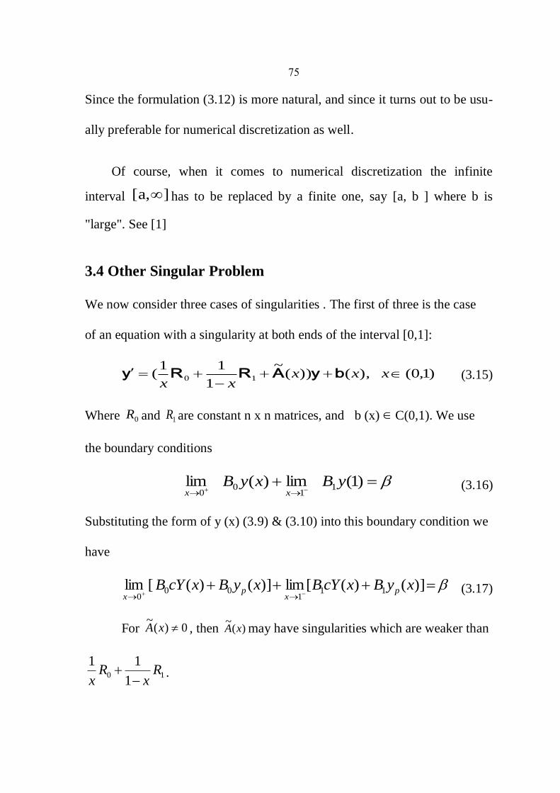
Since the formulation (3.12) is more natural, and since it turns out to be usu-
ally preferable for numerical discretization as well.
Of course, when it comes to numerical discretization the infinite
interval ][a, has to be replaced by a finite one, say [a, b ] where b is
"large". See [1]
3.4 Other Singular Problem
We now consider three cases of singularities . The first of three is the case
of an equation with a singularity at both ends of the interval [0,1]:
)1,0(),())(~
1
11( 10
xxx
xxbyARRy (3.15)
Where 0R and 1R are constant n x n matrices, and b (x) C(0,1). We use
the boundary conditions
)1(lim)(lim 11
00
yBxyBxx
(3.16)
Substituting the form of y (x) (3.9) & (3.10) into this boundary condition we
have
)]()([lim)]()([lim 111
000
xyBxcYBxyBxcYB px
px
(3.17)
For 0)(~
xA , then )(~
xA may have singularities which are weaker than
101
11R
xR
x .
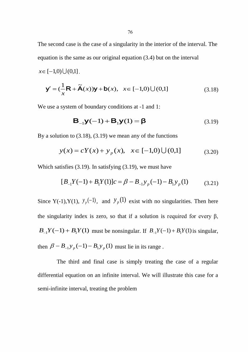
76
The second case is the case of a singularity in the interior of the interval. The
equation is the same as our original equation (3.4) but on the interval
]1,0()0,1[ x .
]1,0()0,1[),())(~1
( xxxx
byARy (3.18)
We use a system of boundary conditions at -1 and 1:
βyByB )1()1( 11 (3.19)
By a solution to (3.18), (3.19) we mean any of the functions
]1,0()0,1[),()()( xxyxcYxy p (3.20)
Which satisfies (3.19). In satisfying (3.19), we must have
)1()1()]1()1([ 1111 pp yByBcYBYB (3.21)
Since Y(-1),Y(1), )1(py , and )1(py exist with no singularities. Then here
the singularity index is zero, so that if a solution is required for every β,
)1()1( 11 YBYB must be nonsingular. If )1()1( 11 YBYB is singular,
then )1()1( 11 pp yByB must lie in its range .
The third and final case is simply treating the case of a regular
differential equation on an infinite interval. We will illustrate this case for a
semi-infinite interval, treating the problem
77
(a) ),0[),()( xxx byAy
(b)
)0()(lim 0 yBxyBx
. (3.22)
If we make the change of variable
11
,1
1
txor
xt (3.23)
We map ),0[ x into )0,1[t . Letting
)11
()(ˆ),11
()(ˆ),11
()(ˆ t
tt
tt
t bbAAyy ,
the problem is then transformed into
(a) )0,1[),(ˆ1)(ˆ)(ˆ1
)(ˆ22
ttt
ttt
t byAy
(b)
)1(ˆ)(ˆlim 00
yBtyBt
(3.24)
Then a necessary and sufficient condition for (3.24) to have at most a
singularity of the first kind at t = 0 is and A (∞) = 0.
This statement implies that if
)1
(1
)(2x
oRx
xA as x → ∞, (3.25)
(3.24) will have exactly a singularity of the first kind if R is not the zero
matrix. See [2]

78
3.5 Finite Difference (Pade Based) Methods
We now describe schemes of finite difference methods based on pade
rational approximation. These methods are based on rational approximants
to the exponential function.
Pade approximants are defined as follows:
Let Czzf ),( ,be function in a region of the complex plane
containing the origin z = 0.
A pade approximant. )(, zR to the function f (z) is defined as by:
)(
)()(
zQ
zPzf
,where )(zP and )(zQ , are polynomials of degrees
κ and μ respectively.
For the function ze)z(f , the polynomials )(zP and )(zQ , are given
explicitly as:
)()!(!)!(
!)!()(
0
j
j
zjj
jzP
And
)()!(!)!(
!)!()(
0
j
j
zjj
jzQ

79
If )()(
)(, zT
zQ
zPe z
, then the remainder )(, zT is given
by:
1
0
)1())1(()1(1
,)()!(
)1()( due
zQ
zzT uuuz
The Pade approximants for ze)z(f (for =1,2,3,4. and κ =1,2,3,4)
Can be generated from the above equations .
Example : When κ = 0 & μ = 2 we will have
2
2
11
1
zz
e z
See Appendix for more function approximations.

81
3.5.1 A Numerical Method Based on The (2,0) Pade
Approximant
Consider the linear second order BVP (2.11). let y o= y, y1= y' then (2.11)
can be written as the system of first order differential equations:
ry
y
pqy
y 010
'
'
1
0
1
0
Which can be written in vector-matrix form as:
D y = Q y + P
With boundary conditions y0 (0) = A , y1 (1) = B. See [10]
To solve this class of singular BVP
B)1(y,A)0(y,1x0),y,x(f)''yx( (3.26)
In which 0 < α ≤ 1 and A, B are finite constants.
)y,x(f'yx
x''y
1
This problem can be written in vector-matrix form as
p y Q y D (3.27)
With special case that is 0p .

80
The boundary conditions become ByAy )1(,)0( 10 . Using the
relation, )x(ye)hx(y hD and replacing the exponential term by its (2,0)
Pade approximant, we get
)x(y)Dy(D2
hhDyI
)h(o)x(y)hx(y]D2
hhDI[
2
322
Using (3.27) and its second derivative and applying the resulting equation to
the discrete point, of Ω (where Ω is the grid
bxx.,,.........xxxa 1NN210 obtained by discretizing the interval
[a, b] into N+1 subintervals each of width *zN
1N
abh
) leads to
the finite-difference formula:
),.....,2,1,0(,11 Nkkkkk 0yByA (3.28)
Where I,IBk is the identity matrix, T
k0k1k ]y,y[y and the
elements of the matrix 1KA are
2,2,11,2,1
2,1,11,1,1
1KAkk
kk
aa
aa
Such that

82
qh
a
phha
pqqh
hqa
qpph
hpa
k
k
k
k
21
2
)'(2
)'(2
1
2
2,2,1
2
1,2,1
2
2,1,1
22
1,1,1
Here the functions p, q and their first derivatives are functions of the
independent discrete points 1kx .
After the vector-matrix equation (3.28) has been applied to the discrete
points ofxxxx N ,.,,.........,, 210 ,the result is a system linear equations
with 2 (N+1) equations in 2 (N+1) unknowns:
A Y = G
Where
1
32
21
01
NN AB
AB
AB
BA
A

83
KA and KB (k = 1,2,…,N) are as defined in (3.28)
T
Nyyy ].,,.........,[ 121 Y , where ),....,2,1(],[ 01 Nkyy T
kkk y .
The last vector T
NN yy ],[ 101,11 y and in this case the two matrices
0B and 1NA will be defined as
00
10B0 and
0
0
1,2,1
1,1,1
1
N
N
Na
aA
respectively.
The vector G is defined by
T
NNN
T
k
NNyayaand
yNk
],[
],0[),,.....,4,3,2(,
11
0
02,2,102,1,11
01
g
g0g
.
3.5.2 A Numerical Method Based on The(3,0)Pade
Approximant
Using the relation )x(ye)hx(y hD and replacing the exponential term
by its (3,0) Pade approximant gives:
)h(o)x(y)hx(y]D)6
h(D)
2
h(hDI[ 43
32
2
Using (3.27) and its second and third derivatives leads to the finite difference
method
),.....,2,1,0(,11 Nkkkkk 0yByA (3.29)
84
Where I,IBK is the identity matrix, T
k kkyyy ],[ 01 and the
elements of the matrix 1kA are
)'(62
1
)'(62
)''2''(6
)'(2
)2'2'3''(6
)'(2
1
32
2,2),1(
232
1,2),1(
2232
2,1),1(
33
22
1,1)1(
pqqh
qh
a
qpph
ph
ha
qqppqqpqh
pqqh
hqa
pqpqppph
qpph
hpa
k
k
k
k
Here the functions p, q and their first and second derivatives are functions of
the independent variable x at the discrete point 1kx .
After applying the vector-matrix equation (3.29) to the discrete points
Nxxxx .,,.........,, 210 . We obtain the system of linear equations with
2 (N+1) equations in 2 (N+1) unknowns:
A y = G
Where kA and kB are as defined in (3.29). The 2(N+1) vector
T
Nyyyyy ].,,.........,,[ 210 contains the 2 x 1 sub-vectors
)N,.....,2,1,0k(yk , where T
k kkyyy ],[ 01 .
85
The last sub-vectors in y is T
N yyyN
],[01 111
. Its structure depends on
the type of boundary conditions. Also in this case the two matrices 0B and
1NA are defined respectively as :
00
10B0 and
0
0
1,2),1(
1,1),1(
1
N
N
Na
aA
The vector T
NgggG ].,,.........,[ 121 contains the sub-vectors
),.....,2,1,0(, Nkk 0g . The first and last sub-vectors 1g
and 1Ng are updated, because of the boundary conditions , to
Ty ],0[001 g and
T
NNN NNyaya ],[
12,212,1 0)1(0)1(1 g respectively.
See [4]&[10]

86
Example 3.1
10,)1()( )2( xyxxyx
With boundary conditions y (0) = 1, y (1) = e.
With α = 0.5 and β = 4,
Which has the exact solution y (x) = xe , this problem is linear and it has
singularity at x = 0 , The value listed as iw approximates and )( ixy is the
exact solution and iee is the error between the exact solution and the
approximate solution. Applying algorithm 2.3 to this problem the solutions
results in table (3.1) , program 8

87
Table (3.1) : The approximate and exact solution for example 3.1.
ix iw iy )()( iii xyxwee
0.00000 1.000000 1.000000 0.000000
0.06250 1.002787 1.000015 0.002772
0.12500 1.004631 1.000244 0.004387
0.18750 1.006828 1.001236 0.005592
0.25000 1.010477 1.003913 0.006563
0.31250 1.016962 1.009582 0.007379
0.37500 1.028057 1.019972 0.008085
0.43750 1.046027 1.037315 0.008711
0.50000 1.073772 1.064494 0.009278
0.56250 1.115088 1.105295 0.009792
0.62500 1.175092 1.164844 0.010247
0.68750 1.260930 1.250325 0.010604
0.75000 1.382958 1.372187 0.010771
0.81250 1.556749 1.546209 0.010540
0.87500 1.806589 1.797113 0.009475
0.93750 2.171762 2.165120 0.006641
1.00000 2.718281 2.718281 0.000000
The maximum error is 0.010771

88
Figure (9): shows the approximate and the exact solution for example (3.1) that was
solved by finite difference method.

89
Applying algorithm 2.1 to example 3.1 ,The results of the calculations with
N =10 and h = 0.1 are given in table (3.2).
Table (3.2) : The approximate and exact solution for example 3.1.
ix iw iy )()( iii xyxwee
0.000 1.000000 1.000100 0.000100
0.100 1.009164 1.000100 0.009064
0.200 1.018424 1.001601 0.016823
0.300 1.030473 1.008132 0.022340
0.400 1.052422 1.025930 0.026491
0.500 1.094095 1.064494 0.029601
0.600 1.170135 1.138372 0.031762
0.700 1.304094 1.271376 0.032718
0.800 1.537564 1.506215 0.031348
0.900 1.951364 1.927261 0.024103
1.000 2.718281 2.718281 0.000000
The maximum error is 0.032718

91
Figure (10): shows the approximate and the exact solution for example (3.1) that was
solved by shooting method.
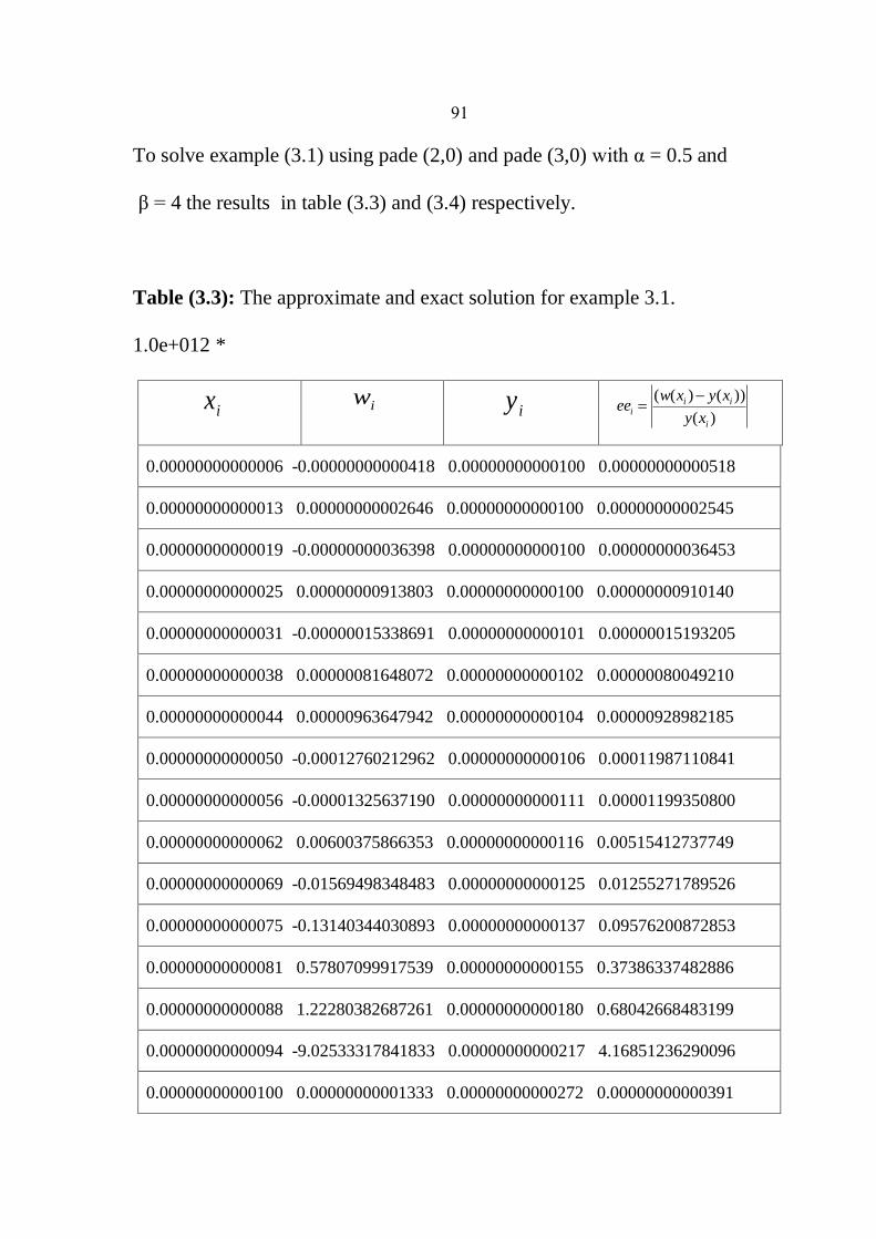
90
To solve example (3.1) using pade (2,0) and pade (3,0) with α = 0.5 and
β = 4 the results in table (3.3) and (3.4) respectively.
Table (3.3): The approximate and exact solution for example 3.1.
1.0e+012 *
ix iw iy
)(
))()((
i
iii
xy
xyxwee
0.00000000000006 -0.00000000000418 0.00000000000100 0.00000000000518
0.00000000000013 0.00000000002646 0.00000000000100 0.00000000002545
0.00000000000019 -0.00000000036398 0.00000000000100 0.00000000036453
0.00000000000025 0.00000000913803 0.00000000000100 0.00000000910140
0.00000000000031 -0.00000015338691 0.00000000000101 0.00000015193205
0.00000000000038 0.00000081648072 0.00000000000102 0.00000080049210
0.00000000000044 0.00000963647942 0.00000000000104 0.00000928982185
0.00000000000050 -0.00012760212962 0.00000000000106 0.00011987110841
0.00000000000056 -0.00001325637190 0.00000000000111 0.00001199350800
0.00000000000062 0.00600375866353 0.00000000000116 0.00515412737749
0.00000000000069 -0.01569498348483 0.00000000000125 0.01255271789526
0.00000000000075 -0.13140344030893 0.00000000000137 0.09576200872853
0.00000000000081 0.57807099917539 0.00000000000155 0.37386337482886
0.00000000000088 1.22280382687261 0.00000000000180 0.68042668483199
0.00000000000094 -9.02533317841833 0.00000000000217 4.16851236290096
0.00000000000100 0.00000000001333 0.00000000000272 0.00000000000391
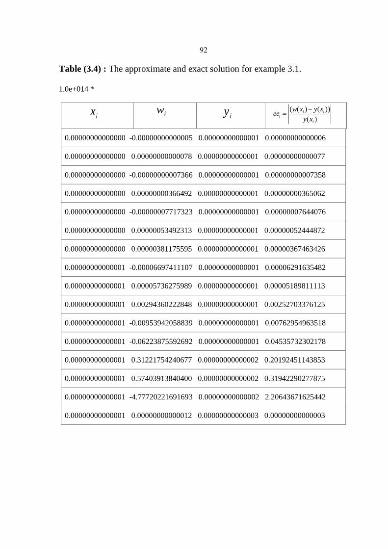
92
Table (3.4) : The approximate and exact solution for example 3.1.
1.0e+014 *
ix iw iy
)(
))()((
i
iii
xy
xyxwee
0.00000000000000 -0.00000000000005 0.00000000000001 0.00000000000006
0.00000000000000 0.00000000000078 0.00000000000001 0.00000000000077
0.00000000000000 -0.00000000007366 0.00000000000001 0.00000000007358
0.00000000000000 0.00000000366492 0.00000000000001 0.00000000365062
0.00000000000000 -0.00000007717323 0.00000000000001 0.00000007644076
0.00000000000000 0.00000053492313 0.00000000000001 0.00000052444872
0.00000000000000 0.00000381175595 0.00000000000001 0.00000367463426
0.00000000000001 -0.00006697411107 0.00000000000001 0.00006291635482
0.00000000000001 0.00005736275989 0.00000000000001 0.00005189811113
0.00000000000001 0.00294360222848 0.00000000000001 0.00252703376125
0.00000000000001 -0.00953942058839 0.00000000000001 0.00762954963518
0.00000000000001 -0.06223875592692 0.00000000000001 0.04535732302178
0.00000000000001 0.31221754240677 0.00000000000002 0.20192451143853
0.00000000000001 0.57403913840400 0.00000000000002 0.31942290277875
0.00000000000001 -4.77720221691693 0.00000000000002 2.20643671625442
0.00000000000001 0.00000000000012 0.00000000000003 0.00000000000003
93
The function bvp4c solves a class of singular BVPs of the form
It can also accommodate unknown parameters for problems of the form
Singular problems must be posed on an interval [0,b] with b>0. Use bvpset
to pass the constant matrix to bvp4c as the value of the 'SingularTerm'
integration property. Boundary conditions at x = 0 must be consistent with
the necessary condition for a smooth solution, Sy(0) = 0. An initial guess
should also satisfy this necessary condition.
When you solve a singular BVP in Matlab using
sol = bvp4c(@odefun,@bcfun,solinit,options)
bvp4c requires that your function odefun(x, y) return only the value of the
f (x, y) term.

94
Example 3.2
Emden's equation. Emden's equation arises in modeling a spherical body
of gas. The PDE of the model is reduced by symmetry to the ODE
on an interval . The coefficient 2 / x is singular at x = 0, but symmetry
implies the boundary condition y'(0) = 0. With this boundary condition, the
term
is well-defined as x approaches 0. For the boundary condition ,
this BVP has the solution
Rewrite the problem as a first-order system and identify the singular
term. Using a substitution yy 1 and yy 2 , write the differential
equation as a system of two first-order equations
The boundary conditions become
Writing the ODE system in a vector-matrix form

95
the terms are identified as
and
Code the ODE and boundary condition functions. Code the differential
equation and the boundary conditions as functions that bvp4c can use.
function dydx = emdenode(x,y)
dydx = [ y(2)
-y(1)^5 ];
function res = emdenbc(ya,yb)
res = [ ya(2)
yb(1) - sqrt(3)/2 ];
Setup integration properties. Use the matrix as the value of the 'Singular
Term' integration property.
S = [0,0;0,-2];
options = bvpset('SingularTerm',S);

96
Create an initial guess. This example starts with a mesh of five points and a
constant guess for the solution.
Use bvpinit to form the guess structure
guess = [sqrt(3)/2;0];
solinit = bvpinit(linspace(0,1,5),guess);
Solve the problem in Matlab. Use the standard bvp4c syntax to solve the
problem.
sol = bvp4c(@emdenode,@emdenbc,solinit,options);
View the results. This problem has solution
The example evaluates the solution at 100 equally spaced points and plots it
along with the numerical solution computed using bvp4c.
x = linspace(0,1);
truy = 1 ./ sqrt(1 + (x.^2)/3);
plot(x,truy,sol.x,sol.y(1,:),'ro');
title('Emden problem -- BVP with singular term.')
legend('Computed');
xlabel('x');
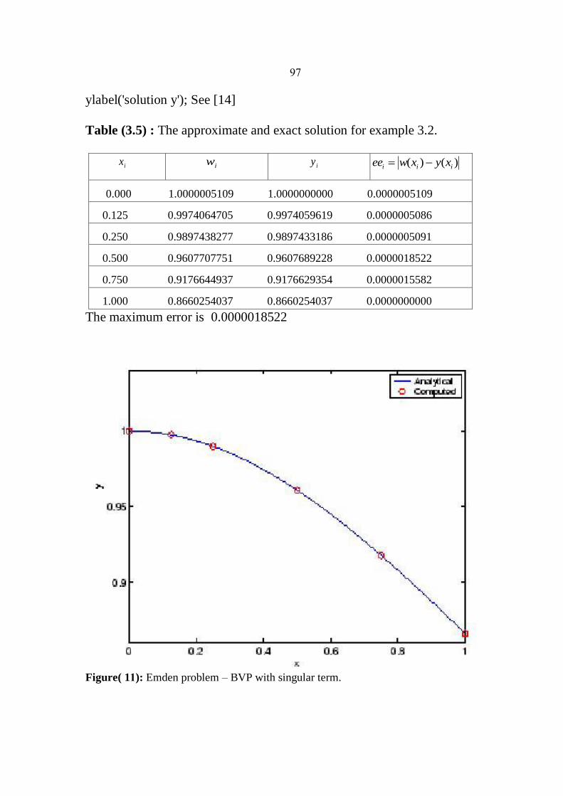
97
ylabel('solution y'); See [14]
Table (3.5) : The approximate and exact solution for example 3.2.
ix iw iy )()( iii xyxwee
0.000 1.0000005109 1.0000000000 0.0000005109
0.125 0.9974064705 0.9974059619 0.0000005086
0.250 0.9897438277 0.9897433186 0.0000005091
0.500 0.9607707751 0.9607689228 0.0000018522
0.750 0.9176644937 0.9176629354 0.0000015582
1.000 0.8660254037 0.8660254037 0.0000000000
The maximum error is 0.0000018522
Figure( 11): Emden problem – BVP with singular term.
98
Conclusion and Results
Various numerical methods namely: Finite Difference, Shooting, Pade
Approximant, have been studied to compare the efficiency of these methods.
It is desirable to develop the results to Pade Approximant to obtain more
accurate for the approximate solution.
From the above work, we see that shooting method is more accurate
for non-linear problems, on the other hand, finite difference method is more
accurate for linear problems.

99
Appendix

011
Matlab Programs
Program 1:
format long
`
clc
a=1;
b=2;
h=1/10;
n=10;
x(1)=1;
m(1)=1;
w(1)=0;
m1(1)=0;
w1(1)=1;
k=zeros(4,2);
for i=1:n
k(1,1)=h*w(i);
k(1,2)=h*[(-2/x(i))*w(i)+(2/(x(i))^2)*m(i)+(sin(log(x(i))))/(x(i))^2];
k(2,1)=h*[w(i)+(1/2)*k(1,2)];
k(2,2)=h*[(-(2/(x(i)+(h/2))))*(w(i)+(1/2)*k(1,2))+(2/(x(i)+(h/2))^2)*
(m(i)+(1/2)*k(1,1))+(sin(log(x(i)+(h/2))))/(x(i))^2];
k(3,1)=h*[w(i)+(1/2)*k(2,2)];
k(3,2)=h*[(-(2/(x(i)+(h/2))))*(w(i)+(1/2)*k(2,2))+(2/(x(i)+(h/2))^2)*
(m(i)+(1/2)*k(2,1))+(sin(log(x(i)+(h/2))))/(x(i))^2];;

010
k(4,1)=h*[w(i)+(1/2)*k(3,2)];
k(4,2)=h*[(-(2/(x(i)+(h))))*(w(i)+k(3,2))+(2/(x(i)+(h))^2)*
(m(i)+k(3,1))+(sin(log(x(i)+(h))))/(x(i))^2];
m(i+1)=m(i)+(1/6)*(k(1,1)+2*k(2,1)+2*k(3,1)+k(4,1));
w(i+1)=w(i)+(1/6)*(k(1,2)+2*k(2,2)+2*k(3,2)+k(4,2));
x(i+1)=a+h*i;
end
kk=zeros(4,2);
for i=1:n
kk(1,1)=h*w1(i);
kk(1,2)=h*[(-2/x(i))*w1(i)+(2/(x(i))^2)*m1(i)];
kk(2,1)=h*[w1(i)+(1/2)*k(1,2)];
kk(2,2)=h*[(-(2/(x(i)+(h/2))))*(w1(i)+(1/2)*k(1,2))+(2/(x(i)+(h/2))^2)
*(m1(i)+(1/2)*k(1,1))];
kk(3,1)=h*[w1(i)+(1/2)*k(2,2)];
kk(3,2)=h*[(-(2/(x(i)+(h/2))))*(w1(i)+(1/2)*k(2,2))+(2/(x(i)+(h/2))^2)
*(m1(i)+(1/2)*k(2,1))];
kk(4,1)=h*[w1(i)+(1/2)*k(3,2)];
kk(4,2)=h*[(-(2/(x(i)+(h))))*(w1(i)+k(3,2))+(2/(x(i)+(h))^2)
*(m1(i)+k(3,1))];
m1(i+1)=m1(i)+(1/6)*(kk(1,1)+2*kk(2,1)+2*kk(3,1)+kk(4,1));
w1(i+1)=w1(i)+(1/6)*(kk(1,2)+2*kk(2,2)+2*kk(3,2)+kk(4,2));
end
012
y=m+((2-m(n+1))/m1(n+1))*m1;
for j=1:n+1
yy(j)=1.1392070132*x(j)+(-0.03920701320/(x(j))^2)-
(3/10)*sin(log(x(j)))-(1/10)*cos(log(x(j)));
ee(j)=abs(y(j)-yy(j));
end
[x' y' yy' ee']
plot (x,y,x,yy)
legend('Approx. Sol.','Exact Sol.');
Program 2
format long
clear
clc
a=0;
b=1;
h=1/20;
n=20;
x(1)=0;
m(1)=0;
w(1)=0;
m1(1)=0;
w1(1)=1;
k=zeros(4,2);

013
for i=1:n
k(1,1)=h*w(i);
k(1,2)=h*[(0)*w(i)+(4)*m(i)+(-4*(x(i)))];
k(2,1)=h*[w(i)+(1/2)*k(1,2)];
k(2,2)=h*[(0)+(4)*(m(i)+(1/2)*k(1,1))-(4*(x(i)+(h/2)))];
k(3,1)=h*[w(i)+(1/2)*k(2,2)];
k(3,2)=h*[(0)+(4)*(m(i)+(1/2)*k(2,1))-(4*(x(i)+(h/2)))];;
k(4,1)=h*[w(i)+(1/2)*k(3,2)];
k(4,2)=h*[(0)+(4)*(m(i)+k(3,1))-(4*(x(i)+h))];
m(i+1)=m(i)+(1/6)*(k(1,1)+2*k(2,1)+2*k(3,1)+k(4,1));
w(i+1)=w(i)+(1/6)*(k(1,2)+2*k(2,2)+2*k(3,2)+k(4,2));
x(i+1)=a+h*i;
end
kk=zeros(4,2);
for i=1:n
kk(1,1)=h*w1(i);
kk(1,2)=h*[(0)+4*m1(i)];
kk(2,1)=h*[w1(i)+(1/2)*kk(1,2)];
kk(2,2)=h*[0+(4)*(m1(i)+(1/2)*kk(1,1))];
kk(3,1)=h*[w1(i)+(1/2)*kk(2,2)];
kk(3,2)=h*[(0)+(4)*(m1(i)+(1/2)*kk(2,1))];
kk(4,1)=h*[w1(i)+(1/2)*kk(3,2)];
kk(4,2)=h*[(0)+(4)*(m1(i)+kk(3,1))];
m1(i+1)=m1(i)+(1/6)*(kk(1,1)+2*kk(2,1)+2*kk(3,1)+kk(4,1));

014
w1(i+1)=w1(i)+(1/6)*(kk(1,2)+2*kk(2,2)+2*kk(3,2)+kk(4,2));
end
y=m+((2-m(n+1))/m1(n+1))*m1;
for j=1:n+1
yy(j)=(exp(1))^(2)*(((exp(1))^(4)-1)^(-1))*((exp(1))^(2*x(j))-((exp(1))^(-
2*x(j))))+x(j);
ee(j)=y(j)-yy(j);
end
[x' y' yy' ee']
plot (x,y,x,yy)
legend('Approx. Sol.','Exact Sol.');
program 3
% To approximate the solution of the nonlinear boundary-value problem
% Y'' = F(X,Y,Y'), A<=X<=B, Y(A) = ALPHA, Y(B) = BETA:
% INPUT: Endpoints A,B; boundary conditions ALPHA, BETA; number
%of subintervals N; tolerance TOL; maximum number of iterations M.
% OUTPUT: Approximations W(1,I) TO Y(X(I)); W(2,I) TO Y'(X(I))
% for each I=0,1,...,N or a message that the maximum number of iterations
was exceeded.
syms('OK', 'A', 'B', 'ALPHA', 'BETA', 'TK', 'AA', 'N');
syms('TOL', 'NN', 'FLAG', 'NAME', 'OUP', 'H', 'K', 'W1' ,'YY1','EE');
syms('W2', 'U1', 'U2', 'I', 'X', 'T', 'K11', 'K12', 'K21');
syms('K22', 'K31', 'K32', 'K41', 'K42', 'J', 's', 'x', 'y', 'z');

015
TRUE = 1;
FALSE = 0;
fprintf(1,'This is the Nonlinear Shooting Method.\n');
fprintf(1,'Input the function F(X,Y,Z) in terms of x, y, z.\n');
fprintf(1,'followed by the partial of F with respect to y on the \n');
fprintf(1,'next line followed by the partial of F with respect to \n');
fprintf(1,'z or y-prime on the next line. \n');
fprintf(1,'actual solution .\n');
fprintf(1,'For example: (32+2*x^3-y*z)/8 \n');
fprintf(1,' -z/8 \n');
fprintf(1,' -y/8 \n');
fprintf(1,' x^2+16/x \n');
s = input(' ','s');
F = inline(s,'x','y','z');
s = input(' ','s');
FY = inline(s,'x','y','z');
s = input(' ','s');
FYP = inline(s,'x','y','z');
s = input(' ','s');
YY11 = inline(s,'x','y','z');
OK = FALSE;
while OK == FALSE
fprintf(1,'Input left and right endpoints on separate lines.\n');
A = input(' ');
016
B = input(' ');
if A >= B
fprintf(1,'Left endpoint must be less than right endpoint.\n');
else OK = TRUE;
end;
end;
fprintf(1,'Input Y(%.10e).\n', A);
ALPHA = input(' ');
fprintf(1,'Input Y(%.10e).\n', B);
BETA = input(' ');
TK = (BETA-ALPHA)/(B-A);
fprintf(1,'TK = %.8e\n', TK);
fprintf(1,'Input new TK? Enter Y or N.\n');
AA = input(' ','s');
if AA == 'Y' | AA == 'y'
fprintf(1,'input new TK\n');
TK = input(' ');
end;
OK = FALSE;
while OK == FALSE
fprintf(1,'Input an integer > 1 for the number of subintervals.\n');
N = input(' ');
if N <= 1
fprintf(1,'Number must exceed 1.\n');
017
else
OK = TRUE;
end;
end;
OK = FALSE;
while OK == FALSE
fprintf(1,'Input Tolerance.\n');
TOL = input(' ');
if TOL <= 0
fprintf(1,'Tolerance must be positive.\n');
else
OK = TRUE;
end;
end;
OK = FALSE;
while OK == FALSE
fprintf(1,'Input maximum number of iterations.\n');
NN = input(' ');
if NN <= 0
fprintf(1,'Must be positive integer.\n');
else
OK = TRUE;
end;
end;

018
if OK == TRUE
fprintf(1,'Choice of output method:\n');
fprintf(1,'1. Output to screen\n');
fprintf(1,'2. Output to text File\n');
fprintf(1,'Please enter 1 or 2.\n');
FLAG = input(' ');
if FLAG == 2
fprintf(1,'Input the file name in the form - drive:\\name.ext\n');
fprintf(1,'for example A:\\OUTPUT.DTA\n');
NAME = input(' ','s');
OUP = fopen(NAME,'wt');
else
OUP = 1;
end;
fprintf(OUP, 'NONLINEAR SHOOTING METHOD\n\n');
fprintf(OUP, ' X(I) W1(I) YY1(I) EE(I)\n');
% STEP 1
W1 = zeros(1,N+1);
W2 = zeros(1,N+1);
H = (B-A)/N;
K = 1;
% TK already computed
OK = FALSE;
% STEP 2
019
while K <= NN & OK == FALSE
% STEP 3
W1(1) = ALPHA;
W2(1) = TK;
U1 = 0 ;
U2 = 1;
% STEP 4
% Runge-Kutta method for systems is used in STEPS 5 and 6
for I = 1 : N
% STEP 5
X = A+(I-1)*H;
T = X+0.5*H;
% STEP 6
K11 = H*W2(I);
K12 = H*F(X,W1(I),W2(I));
K21 = H*(W2(I)+0.5*K12);
K22 = H*F(T,W1(I)+0.5*K11,W2(I)+0.5*K12);
K31 = H*(W2(I)+0.5*K22);
K32 = H*F(T,W1(I)+0.5*K21,W2(I)+0.5*K22);
K41 = H*(W2(I)+K32);
K42 = H*F(X+H,W1(I)+K31,W2(I)+K32);
W1(I+1) = W1(I)+(K11+2*(K21+K31)+K41)/6;
W2(I+1) = W2(I)+(K12+2*(K22+K32)+K42)/6;
K11 = H*U2;
001
K12 = H*(FY(X,W1(I),W2(I))*U1+FYP(X,W1(I),W2(I))*U2);
K21 = H*(U2+0.5*K12);
K22=H*(FY(T,W1(I),W2(I))*(U1+0.5*K11)+FYP(T,W1(I),W2(I))*(U2+0.
5*K21));
K31 = H*(U2+0.5*K22);
K32=H*(FY(T,W1(I),W2(I))*(U1+0.5*K21)+FYP(T,W1(I),W2(I))*(U2+0.
5*K22));
K41 = H*(U2+K32);
K42=H*(FY(X+H,W1(I),W2(I))*(U1+K31)+FYP(X+H,W1(I),W2(I))*(U2+
K32));
U1 = U1+(K11+2*(K21+K31)+K41)/6;
U2 = U2+(K12+2*(K22+K32)+K42)/6;
end;
% STEP 7
% test for accuracy
if abs(W1(N+1)-BETA) < TOL
% STEP 8
I = 0;
Fprintf(OUP, '%3d %13.8f %13.8f %13.8f\n', I, A, ALPHA, TK);
for I = 1 : N
J = I+1;
X = A+I*H;

000
YY1(J)=YY11(X,W1(J),W2(J));
EE(J)=abs(YY1(J)-W1(J));
Fprintf(OUP, ' %13.8f %13.8f %13.8f %13.8f \n', X, W1(J),
YY1(J),EE(J));
end;
fprintf(OUP, 'Convergence in %d iterations\n', K);
fprintf(OUP, ' t = %14.7e\n', TK);
% STEP 9
OK = TRUE;
else
% STEP 10
% Newton's method applied to improve TK
TK = TK-(W1(N+1)-BETA)/U1;
K = K+1;
end;
end;
% STEP 11
% method failed
if OK == FALSE
fprintf(OUP, 'Method failed after %d iterations\n', NN);
end;
end;
if OUP ~= 1
fclose(OUP);
002
fprintf(1,'Output file %s created successfully \n',NAME);
end;
program 4
format long
clear
clc
a=1;
b=2;
h=1/10;
n=11;
y=zeros(10,1);
for i=1:10
x(i)=a+(i)*h;
yy(i)=1.1392070132*x(i)+(-0.03920701320/(x(i)^2))-
(3/10)*sin(log(x(i)))-(1/10)*cos(log(x(i)));
end
[x' yy'];
u=zeros(9,9);
bb=zeros(9,1);
u(1,1)=-((2*(h)^2/(x(1))^(2))+2);
u(1,2)=(1+(h/x(1)));
u(2,1)=(1-(h/x(2)));
bb(1)=((h)^2)*sin(log(x(1)))/(x(1))^(2)-(1-(h/x(1)));
for j=2:8

003
for k=2:8
if j==k
u(j,k)=-1*((2*(h)^(2)/(x(j))^(2))+2);
elseif j==k+1
u(j,k)=(1-(h/x(j)));
elseif j==k-1
u(j,k)=(1)+(h/x(j));
else u(j,k)=0;
end
end
end
u(9,8)=(1-(h/x(9)));
u(9,9)=-(2*(h)^(2)/(x(9))^(2)+2);
u(8,9)=(1+(h/x(8)));
u;
for oo=2:8
ll(oo)=log(x(oo));
bb(oo)=((h)^(2)*sin(ll(oo)))/(x(oo))^(2);
end
bb(9)=((h)^2)*sin(log(x(9)))/(x(9))^(2)-(2*(1+(h/x(9))));
[L U]=lu(u);
z=inv(L)*bb;
y=inv(U)*z;
y(10)=2;

004
for rr=1:10
ee(rr)=abs(y(rr)-yy(rr));
end
[x' y yy' ee']
plot(x,y,x,yy);
xlabel('Time');
legend('Approx. Sol.','Exact Sol.');
program 5
clc
clear
format long
a=0;
b=1;
n=19;
h=1/20;
y=zeros(20,1);
%y(1)=1;
for i=1:20
x(i)=a+(i)*h;
end
for jj=1:20
yy(jj)=(exp(1))^(2)*(((exp(1))^(4)-1)^(-1))*((exp(1))^(2*x(jj))-
((exp(1))^(-2*x(jj))))+x(jj);
005
end
[x' yy'];
u=zeros(19,19);
bb=zeros(19,1);
u(1,1)=-(2+(4*(h)^2));
u(1,2)=(1);
u(2,1)=(1);
bb(1)=(-4*x(1)*(h)^(2));
for j=2:18
for k=2:18
if j==k
u(j,k)=-1*(2+(4*(h)^(2)));
elseif j==k+1
u(j,k)=(1);
elseif j==k-1
u(j,k)=(1);
else u(j,k)=0;
end
end
end
u(19,18)=(1);
u(19,19)=-(2+(4*(h)^(2)));
u(18,19)=(1);
u;

006
for oo=2:18
bb(oo)=(-4*(x(oo))*(h)^(2));
end
bb(19)=(-4*(x(oo))*(h)^(2))-2;
bb;
[L U]=lu(u);
z=inv(L)*bb;
y=inv(U)*z;
y(20)=2;
for rr=1:20
ee(rr)=abs(y(rr)-yy(rr));
end
[x' y yy' ee']
plot(x,y,x,yy);
xlabel('Time');
legend('Approx. Sol.','Exact Sol.');
program 6
clc
format long
clear
a=1;
b=3;
y0=17;

007
h=0.1;
n=(b-a)/h-1;
yn=(43/3);
x=[a+h:h:b-h];
y=17*ones(n,1);k=1;
c=zeros(n,1);j=zeros(19,19);m=50;
while norm (c-y ,inf)>0.000001
%finding he jacobian matrix
j(1,1)=-2+(1/16)*h*(y(2)-y0);
j(1,2)=1+(1/16)*h*y(1);
for i=2:n-1
for t=2:n-1
if i==t
j(i,t)=-2+(1/16)*h*(y(i+1)-y(i-1));
elseif i==t+1
j(i,t)=1-(1/16)*h*y(i);
elseif i==t-1
j(i,t)=1+(1/16)*h*y(i);
end
end
end
j(n-1,n)=1+(1/16)*h*y(n-1);
j(n,n-1)=1-(1/16)*h*yn;

008
j(n,n)=-2+(1/16)*h*yn-(1/8)*h*y(n-1);
%====================================================
f(1,1)=(y(2)-2*y(1)+y0)-((h)^(2)/8)*(32+(2*(x(1).^3))-(y(1)*((y(2)-
y0)/(2*h))));
for i=2:n-1
f(i,1)= (y(i+1)-2*y(i)+y(i-1))-((h)^(2)/8)*(32+(2*(x(i).^3))-
(y(i)*((y(i+1)-y(i-1))/(2*h))));
end
f(n,1)=(yn-2*y(n)+y(n-1))-((h)^(2)/8)*(32+(2*(x(n)^3))-(y(n)*((yn-y(n-
1))/(2*h))));
f;
z=inv(j)*(-1*f);
c=y;
y=y+z;
y
end
xx=[a,x,b];
y1=[y0,y',yn];
for tt=1:n+2
yy(tt)=(xx(tt))^(2)+(16/xx(tt));
e(tt)=abs(y1(tt)-yy(tt));
end
[xx;y1;yy;e]'

009
plot(xx,y1,xx,yy);
xlabel('Time');
legend('Approx. Sol.','Exact Sol.');
program 7
clc
format long
clear
a=1;
b=2;
y0=2;
h=0.1;
n=(b-a)/h-1;
yn=(5/2);
x=[a+h:h:b-h];
y=2*ones(n,1);k=1;
c=zeros(n,1);j=zeros(n,n);m=50;
while norm (c-y ,inf)>0.000001
%finding he jacobian matrix
j(1,1)=((-2/(h)^2)-2*(y(1))^2+6);
j(1,2)=1/(h)^2;
for i=2:n-1
for t=2:n-1
if i==t
021
j(i,t)=((-2/(h)^2)-2*(y(i))^2+6);
elseif i==t+1
j(i,t)=1/(h)^2;
elseif i==t-1
j(i,t)=1/(h)^2;
end
end
end
j(n-1,n)=1/(h)^2;
j(n,n-1)=1/(h)^2;
j(n,n)=((-2/(h)^2)-2*(y(n))^2+6);
%====================================================
f(1,1)=(y(2)-2*y(1)+y0)+((h)^(2))*(-2*(y(1))^3+6*(y(1))+2*(x(1))^3);
for i=2:n-1
f(i,1)= (y(i+1)-2*y(i)+y(i-1))+((h)^(2))*(-
2*(y(i)^3)+6*(y(i))+2*(x(i))^3);
end
f(n,1)=(yn-2*y(n)+y(n-1))+((h)^(2))*(-2*(y(n)^3)+6*(y(n))+2*(x(n))^3);
f;
z=inv(j)*(-1*f);
c=y;
y=y+z;
y;
end
020
xx=[a,x,b];
y1=[y0,y',yn];
for tt=1:n+2
yy(tt)=(xx(tt))+(xx(tt))^(-1);
e(tt)=abs(y1(tt)-yy(tt));
end
[xx;y1;yy;e]'
plot(xx,y1,xx,yy);
xlabel('Time');
legend('Approx. Sol.','Exact Sol.');
program 8
clc
clear
ba=0;
bb=1;
n=15;
h=1/16;
alpha=1;
beta=2.718281828;
aa=0.5;
k=4;
for i=1:n
t(i)=ba+i*h;
022
end
t
for j=1:n
p1((j))=aa/t(j);
q1((j))=(k*(t(j))^(aa+k-2)*(aa+k-1+k*(t(j))^(k)))/(t(j))^(aa);
end
[t' p1' q1']
a(1)=(-4-2*((h)^2)*q1((1)));
c(1)=(2+h*p1((1)));
for i=2:n-1
a(i)=(-4-2*((h)^2)*q1((i)));
c(i)=(2+h*p1((i)));
d(i)=(2-h*p1((i)));
end
a(n)=-4-2*((h)^2)*q1((n));
d(n)=2-h*p1((n));
l(1)=a(1);u(1)=c(1)/l(1);
for i=2:n-1
l(i)=a(i)-d(i)*u(i-1);
u(i)=c(i)/l(i);
end
l(n)=a(n)-d(n)*u(n-1);
dd(1)=-(2-h*p1(1))*alpha;
for i=2:n-1

023
dd(i)=0;
end
dd(n)=-(2+h*p1(n))*beta;
z(1)=dd(1)/l(1);
for i=2:n
z(i)=(dd(i)-d(i)*z(i-1))/l(i);
end
y(n)=z(n);
for i=n-1:-1:1
y(i)=z(i)-u(i)*y(i+1);
end
y
for i=1:n
yy(i)=(2.718281828)^((t(i))^k);
end
yy
for i=1:n
ee(i)=y(i)-yy(i);
end
ee
[t' y' yy' ee']
plot(t',y',t',yy')
legend('Approx. Sol.','Exact Sol.');
024
program 9
format long
clear
clc
a=0;
b=1;
aa=0.5;
k1=4;
h=1/10;
n=10;
x(1)=0.1;
m(1)=1;
w(1)=0;
m1(1)=0;
w1(1)=1;
k=zeros(4,2);
for i=1:n
k(1,1)=h*w(i);
k(1,2)=h*[(-aa/x(i))*w(i)+((((k1*(x(i))^(aa+k1-2))*(aa+k1-
1+k1*(x(i))^(k1)))/(x(i))^(aa))*m(i))+(0*(x(i)))];
k(2,1)=h*[w(i)+(1/2)*k(1,2)];
k(2,2)=h*[(-aa/(x(i)+(h/2)))*(w(i)+(1/2)*k(1,2))+((((k1*((x(i)+(h/2))
^(aa+k1-2))*(aa+k1-1+k1*(x(i)+(h/2))^(k1)))/(x(i)+(h/2))^(aa)))
*(m(i)+(1/2)*k(1,1)))-(0*(x(i)+(h/2)))];

025
k(3,1)=h*[w(i)+(1/2)*k(2,2)];
k(3,2)=h*[(-aa/(x(i)+(h/2)))*(w(i)+(1/2)*k(2,2))+
((((k1*((x(i)+(h/2))^(aa+k1-2))*(aa+k1-1+k1*(x(i)+(h/2))^(k1)))/(x(i)
+(h/2))^(aa)))*(m(i)+(1/2)*k(2,1)))-(0*(x(i)+(h/2)))];;
k(4,1)=h*[w(i)+(1/2)*k(3,2)];
k(4,2)=h*[(-aa/(x(i)+h))*(w(i)+k(3,2))+((((k1*((x(i)+h)^(aa+k1-
2))*(aa+k1-1+k1*(x(i)+h)^(k1)))/(x(i)+h)^(aa)))*(m(i)+k(3,1)))-
(0*(x(i)+h))];;
m(i+1)=m(i)+(1/6)*(k(1,1)+2*k(2,1)+2*k(3,1)+k(4,1));
w(i+1)=w(i)+(1/6)*(k(1,2)+2*k(2,2)+2*k(3,2)+k(4,2));
x(i+1)=a+h*i;
end
x
kk=zeros(4,2);
for i=1:n
kk(1,1)=h*w1(i);
kk(1,2)=h*[(-aa/x(i))*w1(i)+((((k1*(x(i))^(aa+k1-2))*(aa+k1-
1+k1*(x(i))^(k1)))/(x(i))^(aa))*m1(i))];
kk(2,1)=h*[w1(i)+(1/2)*kk(1,2)];
kk(2,2)=h*[(-aa/(x(i)+(h/2)))*(w1(i)+(1/2)*kk(1,2))
+(((((k1*(x(i)+(h/2))^(aa+k1-2))*(aa+k1-1+k1*(x(i)+(h/2))^(k1)))/
(x(i)+(h/2))^(aa)))*(m1(i)+(1/2)*kk(1,1)))];
kk(3,1)=h*[w1(i)+(1/2)*kk(2,2)];
kk(3,2)=h*[(-aa/(x(i)+(h/2)))*(w1(i)+(1/2)*kk(2,2))

026
+((((k1*((x(i)+(h/2))^(aa+k1-2))*(aa+k1-1+k1*(x(i)+(h/2))^(k1)))/
(x(i)+(h/2))^(aa)))*(m1(i)+(1/2)*kk(2,1)))];
kk(4,1)=h*[w1(i)+(1/2)*kk(3,2)];
kk(4,2)=h*[(-aa/(x(i)+h))*(w1(i)+kk(3,2))+((((k1*((x(i)+h)^(aa+k1-
2))*(aa+k1-1+k1*(x(i)+h)^(k1)))/(x(i)+h)^(aa)))*(m1(i)+kk(3,1)))];
m1(i+1)=m1(i)+(1/6)*(kk(1,1)+2*kk(2,1)+2*kk(3,1)+kk(4,1));
w1(i+1)=w1(i)+(1/6)*(kk(1,2)+2*kk(2,2)+2*kk(3,2)+kk(4,2));
end
y=m+(((exp(1))-m(n+1))/m1(n+1))*m1;
for j=1:n+1
yy(j)=(2.718281828)^((x(j))^k1);
ee(j)=abs(y(j)-yy(j));
end
[x' y' yy' ee']
plot (x,y,x,yy)
legend('Approx. Sol.','Exact Sol.');
program 10
%PADE APPROXIMATE METHOD (2,0) TO SOLVE BVP
%((x)^(aa)*y)'=k*x(aa+k-2)*(aa+k-1+k*(x)^k)*y
%0<x<1 y(0)=1 y(1)=e(1)
%=======================================
clc
clear
027
format long
D=[0 1];
n=15;
a=.5;
b=4;
h=(D(2)-D(1))/(n+1);
xx=D(1)+h+[0:h:D(2)-h];
xx
P=inline('-a/x','x','a');
Q=inline('(b*x^(a+b-2)*(a+b-1+b*x^b))/(x^a)','x','a','b');
PP=inline('a/(x^2)','x','a');
QQ=inline('28*x+96*x^5','x');
PPP=inline('-1/(x)','x');
QQQ=inline('28+480*x^4','x');
f=[-1 0;0 -1]
for i=1:1:n+1
aa(1,1)=h*P(xx(i),a)+(h^2*(-PP(xx(i),a)+(P(xx(i),a))^2-
Q(xx(i),a,b)))/2+h^3*(PPP(
xx(i))-3*P(xx(i),a)*PP(xx(i),a)+2*QQ(xx(i))+(P(xx(i),a))^3-
2*P(xx(i),a)*Q(xx(i),a,b))/6;
aa(1,2)=h*Q(xx(i),a,b)+h^2*(-
QQ(xx(i))+P(xx(i),a)*Q(xx(i),a,b))/2+(h^3*(QQQ(xx(i))-2*
028
PP(xx(i),a)*Q(xx(i),a,b)-
P(xx(i),a)*QQ(xx(i))+(P(xx(i),a))^2*Q(xx(i),a,b)-(Q(xx(i),a,b))^2))/6;
aa(2,1)=-h-(h^2*P(xx(i),a))/2+h^3((PP(xx(i),a)-
(P(xx(i),a))^2+Q(xx(i),a,b)))/6;
aa(2,2)=-1*(h^2*Q(xx(i),a,b))/2+h^3(QQ(xx(i))-
P(xx(i),a)*Q(xx(i),a,b))/6;
AA(2*i-1,2*i-1)=aa(1,1);
AA(2*i-1,2*i)=aa(1,2);
AA(2*i,2*i-1)=aa(2,1);
AA(2*i,2*i)=aa(2,2);
end
for r=1:1:n
AA(2*r+1:2*r+2,2*r-1:2*r)=f;
end
AA(1,end)=-1;
AA(end-1,end)=0;
AA(end,end)=0;
AA
G=zeros(2*n+2,1);
G(2)=1;
G(2*n+1)=-1.6035*exp(1);
G(2*n+2)=-0.9414*exp(1);
G;
[l,u]=lu(AA);

029
t=inv(l)*G;
y=inv(u)*t;
y;
y1(1)=y(2)
for jj=4:2: 32 %(2*(n+1))
y1(jj/2)=y(jj);
end
y1
for i=1:n+1
yy(i)=(2.718281828)^((xx(i))^b);
end
yy
for i=1:n+1
ee(i)=abs(yy(i)-y1(i));
end
[xx' y1' yy' ee']
Program 11
%PADE APPROXIMATE METHOD (3,0) TO SOLVE BVP
%((x)^(aa)*y)'=k*x(aa+k-2)*(aa+k-1+k*(x)^k)*y
%0<x<1 y(0)=1 y(1)=e(1)
%=======================================
clc
clear

031
format long
D=[0 1];
n=15;
a=.5;
b=4;
h=(D(2)-D(1))/(n+1);
xx=D(1)+h+[0:h:D(2)-h];
xx
P=inline('-a/x','x','a');
Q=inline('(b*x^(a+b-2)*(a+b-1+b*x^b))/(x^a)','x','a','b');
PP=inline('a/(x^2)','x','a');
QQ=inline('28*x+96*x^5','x');
PPP=inline('-1/(x)','x');
QQQ=inline('28+480*x^4','x');
f=[-1 0;0 -1]
for i=1:1:n+1
aa(1,1)=h*P(xx(i),a)+(h^2*(-PP(xx(i),a)+(P(xx(i),a))^2-
Q(xx(i),a,b)))/2+h^3*(PPP(xx(i))-
3*P(xx(i),a)*PP(xx(i),a)+2*QQ(xx(i))+(P(xx(i),a))^3-
2*P(xx(i),a)*Q(xx(i),a,b))/6;
aa(1,2)=h*Q(xx(i),a,b)+h^2*(-
QQ(xx(i))+P(xx(i),a)*Q(xx(i),a,b))/2+(h^3*(QQQ(xx(i))-
2*PP(xx(i),a)*Q(xx(i),a,b)-
P(xx(i),a)*QQ(xx(i))+(P(xx(i),a))^2*Q(xx(i),a,b)-(Q(xx(i),a,b))^2))/6;

030
aa(2,1)=-h-(h^2*P(xx(i),a))/2+h^3*((PP(xx(i),a)-
(P(xx(i),a))^2+Q(xx(i),a,b)))/6;
aa(2,2)=-1*(h^2*Q(xx(i),a,b))/2+h^3*(QQ(xx(i))-
P(xx(i),a)*Q(xx(i),a,b))/6;
AA(2*i-1,2*i-1)=aa(1,1);
AA(2*i-1,2*i)=aa(1,2);
AA(2*i,2*i-1)=aa(2,1);
AA(2*i,2*i)=aa(2,2);
end
for r=1:1:n
AA(2*r+1:2*r+2,2*r-1:2*r)=f;
end
AA(1,end)=-1;
AA(end-1,end)=0;
AA(end,end)=0;
AA
G=zeros(2*n+2,1);
G(2)=1;
G(2*n+1)=1.5891723*exp(1);
G(2*n+2)=-0.0529378*exp(1);
G;
[l,u]=lu(AA);
t=inv(l)*G;
y=inv(u)*t;
032
y;
y1(1)=y(2)
for jj=4:2: 32 %(2*(n+1))
y1(jj/2)=y(jj);
end
y1
for i=1:n+1
yy(i)=(2.718281828)^((xx(i))^b);
end
yy
for i=1:n+1
ee(i)=abs(yy(i)-y1(i));
end
[xx' y1' yy' ee']
Example
Find pade approximations for x
xf
1
1)( expanded about 00 x
:1
1)(
xxf
x0 = 0;
a = -1.5;
b = 1.5;
c = 0.0;
d = 8.5;
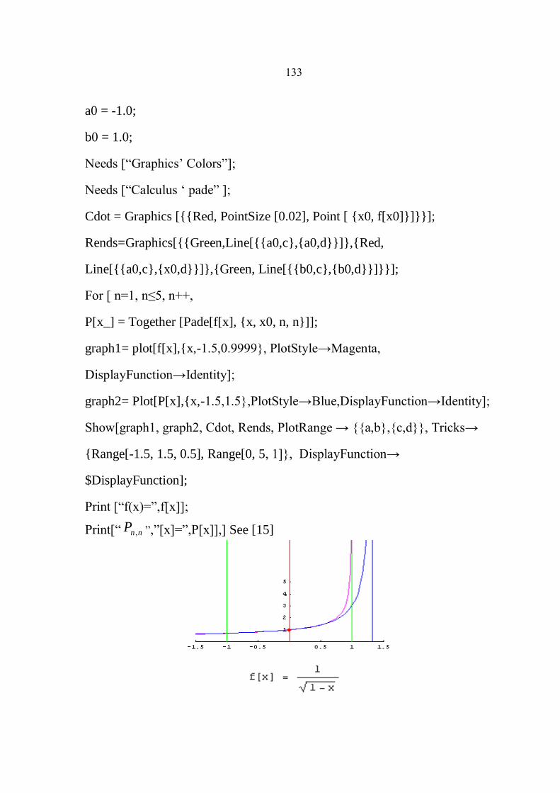
033
a0 = -1.0;
b0 = 1.0;
Needs [“Graphics‟ Colors”];
Needs [“Calculus „ pade” ];
Cdot = Graphics [{{Red, PointSize [0.02], Point [ {x0, f[x0]}]}}];
Rends=Graphics[{{Green,Line[{{a0,c},{a0,d}}]},{Red,
Line[{{a0,c},{x0,d}}]},{Green, Line[{{b0,c},{b0,d}}]}}];
For [ n=1, n≤5, n++,
P[x_] = Together [Pade[f[x], {x, x0, n, n}]];
graph1= plot[f[x],{x,-1.5,0.9999}, PlotStyle→Magenta,
DisplayFunction→Identity];
graph2= Plot[P[x],{x,-1.5,1.5},PlotStyle→Blue,DisplayFunction→Identity];
Show[graph1, graph2, Cdot, Rends, PlotRange → {{a,b},{c,d}}, Tricks→
{Range[-1.5, 1.5, 0.5], Range[0, 5, 1]}, DisplayFunction→
$DisplayFunction];
Print [“f(x)=”,f[x]];
Print[“ nnP , ”,”[x]=”,P[x]],] See [15]
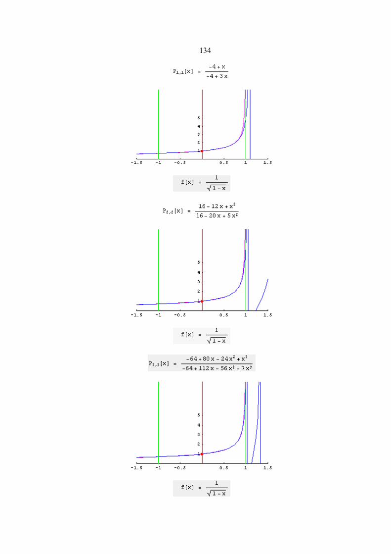
034

035

036
References
[1] Ascher, Mattheij, R.M.M, RUSSELL,r.d, (1995). Numerical Solution
of Boundary Value Problems For Ordinary Dfferential Equations.
[2] Brabston, D.C. (1974). Numerical Solution of Singular Endpoint
Boundary Value Problems, Pasadena, California.
[3] Burden, R.L, Faires,J.D, (2001). Numerical Method, Youngstown
State University, seventh edition.
[4] Butcher, J.C. (2008). Numerical methods for ordinary differential
equations, Wiley.
[5] E1-gebeily, M.A, Attili, B.S,(2003). An Iterative Shooting Method
For a certain Class of Singular Two-point Boundary Value Problems,
King Fahd University of Petroleum And Minerals.
[6] Isaacson.E and keller.H.B,( 1960). Analysis of Numerical Methods,
1NC, Newyourk.
[7] Keller,H.B, (1976). Numerical Solution of Two-point Boundary
Value Problems, California Institute of Technologe.
[8] Leveque,R.J,( 2006). Finite Difference Methods For Differential
Equations, Washington University.
[9] Shampine.L.F, Gladwell.I , Thompson.S, (2003). Solving ODEs with
MATLAB, Cambridge, University Press.
[10] Thompson.P.A.O, (1996).Sequential And Parallel Numerical
Methods For Second Order Two-point Boundary Value Problems;

037
Brunel University.
[11] Twizell,E.I-J,( 1988). Numerical Methods, With Applications In
The Biomedical Sciences, Brunel University.
[12] www.physics.arizona.edu.
[13] www.wikipedia.org.
[14] www.mathworks.com.
[15]www.math.fullerton.edu.
2010

ب
pade approximation methodsshooting method


