
The Pennsylvania State University
The Graduate School
College of Engineering
SIZE EFFECT IN NORMAL AND HIGH-STRENGTH CONCRETE CYLINDERS
SUBJECTED TO STATIC AND DYNAMIC AXIAL COMPRESSIVE LOADS
A Thesis in
Civil Engineering
by
Motaz M. Elfahal
© 2003 Motaz M. Elfahal
Submitted in Partial Fulfillment of the Requirements
for the Degree of
Doctor of Philosophy
May 2003

We approve the thesis of Motaz M. Elfahal. ____________________________________ Theodor Krauthammer Professor of Civil Engineering Thesis Advisor Chair of Committee ___________________________________ Andrea J. Schokker Assistant Professor of Civil Engineering ____________________________________ Kevin L. Koudela Research Associate ____________________________________ Vijay K. Varadan Distinguished Alumni Professor of Engineering Science and Mechanics and Electrical Engineering ____________________________________ Andrew Scanlon Professor of Civil Engineering Head of the Department of Civil and Environmental Engineering
Date of Signature ________________________ ________________________ ________________________ ________________________ ________________________

iii
ABSTRACT
Concrete structures have traditionally been designed on the basis of strength criteria.
This implies that geometrically similar structures of different sizes should fail at the same
nominal stress. However, this is not quite true in many cases because of the Size Effect,
which may be understood as the dependence of the concrete structure on its characteristic
dimension. The actual concrete strength of relatively larger structural members may be
significantly lower than that of the standard size. By neglecting the Size Effect, predicted
load capacity values become increasingly less conservative as a member size increases.
Also, very large structures such as dams, bridges, and foundations are too large and too
strong to be tested at full scale in the laboratory. In recent years, major advances have
been made in understanding of scaling and Size Effect. However, these advances remain
only in the static domain (i.e., slow loading rates), and none of the previous studies have
addressed the effect of higher loading rates or high-strength concrete (HSC) on the Size
Effect. Structural concrete can be subjected to high loading rates, such as those
associated with impact and explosion incidents. Such load conditions are generated by
dropped objects, vehicle collision into structures, accidental industrial explosions, missile
impacts, military explosions, etc. The Size Effect in normal strength concrete (NSC) is a
phenomenon explained by a combination of plasticity and fracture mechanics, and it is
related to the energy balance during the damage/fracture process which causes a change
in the mode of failure of the concrete member with the increase in its size, thus causing a
reduction in its strength. Although structural response and damage evolution are expected
to be size-dependent, it is not clear how time or the material strength affect this
phenomenon. In this study, the Size Effect phenomenon was investigated under
iv
compressive static and impact loads for both normal and high-strength concrete cylinders.
This study was conducted by performing 127 compressive static and impact tests on both
normal and high-strength concrete and 192 numerical simulations. The tests provided
data whose analysis produced evidence on the effect of loading rate and material strength
on the Size Effect for structural concrete in compression. Parallel pre- and post-test
computational simulations were used to perform ‘numerical tests’ of the same specimens,
and to explore the role of the time dimension on the physical phenomena that contribute
to the Size Effect. Comparisons between test and numerical data assisted and guided the
investigators in identifying the governing parameters that define the physical phenomena.
In addition, the precision test data assisted in validating the computational tools used for
the study. This thesis describes this multinational collaborative study (with experimental
tests performed at three different locations: Penn State University, USA; the National
Defense Academy, Japan; and the University of British Colombia, Canada), and it
presents data from both the unique impact tests and the related numerical simulations.
Two material models were developed to simulate the dynamic Size Effect that was
proved to exist in this study. The study also proved the existence of Size Effect in
parameters other than strength such as the modulus of elasticity and the strain at
maximum stress. This necessitated modifying the existing Size Effect which was mainly
confined to the strength parameter only. Use of high-speed photography enabled the
detection of several modes of failure experienced by concrete cylinders subjected to axial
impact.

v
TABLE OF CONTENTS
LIST OF FIGURES .......................................................................................................viii LIST OF TABLES..........................................................................................................xii NOMENCLATURE........................................................................................................xiv ACKNOWLEDGMENTS..............................................................................................xvi CHAPTER ONE INTRODUCTION..............................................................................................................1 1.1 Research Significance ............................................................................................. 1 1.2 Objective and Scope................................................................................................ 2 1.3 Thesis Layout .......................................................................................................... 3 CHAPTER TWO LITERATURE REVIEW..................................................................................................4 2.1 Introduction............................................................................................................. 4 2.2 Classical Definition of Size Effect.......................................................................... 4 2.3 Proposed Modification to the Definition of Size Effect ......................................... 5 2.4 Background ............................................................................................................. 5 2.5 Evidence of Size Effect........................................................................................... 7
2.5.1 Theoretical Evidence........................................................................................................................... 7 2.5.2 Experimental evidence........................................................................................................................ 9
2.5.2.1 Size Effect in Concrete Compressive Strength........................................................................... 9 2.5.2.2 Size Effect in Concrete Tensile Strength..................................................................................... 9 2.5.2.3 Size Effect in Strain Gradient and Cracking Strain ................................................................. 10 2.5.2.4 Size Effect in Ultimate Shear Strength ...................................................................................... 10 2.5.2.5 Size Effect in Diagonal Shear Failure of Beams without Stirrups........................................ 10 2.5.2.6 Torsional failure ............................................................................................................................. 11 2.5.2.7 Punching shear failure of slabs.................................................................................................... 11 2.5.2.8 Pull-out failures .............................................................................................................................. 11 2.5.2.9 Compression failure of tied columns.......................................................................................... 11 2.5.2.10 Three-point bending of beams ..................................................................................................... 11 2.5.2.11 Influence of Specimen Size on Elastic Modulus of Concrete................................................ 12
2.6 Explanation of Size Effect .................................................................................... 12 2.6.1 Statistical Theory ............................................................................................................................... 12 2.6.2 Energy Theory and the Size Effect Law........................................................................................ 14 2.6.3 Boundary Layer Effect...................................................................................................................... 19 2.6.4 Diffusion Phenomena........................................................................................................................ 20 2.6.5 Hydration Heat or Other Phenomena Associated With Chemical Reactions.......................... 22 2.6.6 Influence of aggregate size on Size Effect .................................................................................... 22
2.7 Size Effect in High-Strength Concrete (HSC) ...................................................... 23 2.8 Size Effect in the Dynamic Domain ..................................................................... 24 2.9 Design and Code Issues ........................................................................................ 25 2.10 Summary of Key Issues for this Study ................................................................. 27 CHAPTER THREE METHODOLOGY...........................................................................................................28 3.1 Pre-test Simulations .............................................................................................. 29
3.1.1 Description of the Concrete Constitutive Models ........................................................................ 32 3.2 Tests ...................................................................................................................... 37

vi
3.2.1 Tests on Normal-Strength Concrete (NSC) Cylinders ................................................................ 37 3.2.2 Tests on High-Strength Concrete (HSC) Cylinders ..................................................................... 41 3.2.3 Data Obtained From the Tests ......................................................................................................... 42
3.3 Post-test simulations ............................................................................................. 43 3.4 Statement of Work ................................................................................................ 49 CHAPTER FOUR INSTRUMENTATIONS AND TEST SETUP..............................................................51 4.1 Introduction........................................................................................................... 51 4.2 Drop Hammers ...................................................................................................... 52
4.2.1 Drop hammer at Penn State University.......................................................................................... 52 4.2.2 Drop hammer at NDA, Japan .......................................................................................................... 58 4.2.3 Drop Hammers at UBC, Canada..................................................................................................... 61
4.3 Response Measurement ......................................................................................... 63 4.3.1 Background......................................................................................................................................... 63 4.3.2 Sensors and Transducers .................................................................................................................. 65 4.3.3 Sensor selection.................................................................................................................................. 65
4.3.3.1 Load Cells ....................................................................................................................................... 66 4.3.3.2 Accelerometers............................................................................................................................... 67 4.3.3.3 Strain Gages.................................................................................................................................... 69
4.4 High-Speed Data Acquisition Systems ................................................................. 71 4.4.1 Data Acquisition System at Penn State University (PSU).......................................................... 72 4.4.2 Data Acquisition System at the National Defense Academy (NDA) ....................................... 76 4.4.3 Data acquisition system at the University of British Colombia (UBC).................................... 77
4.5 High-Speed Photography ...................................................................................... 78 CHAPTER FIVE RESULTS AND DISCUSSION – HIGH-STRENGTH CONCRETE.......................80 5.1 Pre-test Simulations .............................................................................................. 80 5.2 Tests ...................................................................................................................... 84 5.3 Comparison of Test and Pre-Test Simulation Results .......................................... 89 5.4 Post-test simulations ............................................................................................. 92 5.5 Results ................................................................................................................... 95 5.6 Discussion of Results ............................................................................................ 97 5.7 Summary of main achievements........................................................................... 99 CHAPTER SIX RESULTS AND DISCUSSION – NORMAL-STRENGTH CONCRETE.............101 6.1 Pre-test Simulations ............................................................................................ 102
6.1.1 Hard Impact Pre -Test Simulations................................................................................................103 6.1.2 Soft Impact Pre-Test Simulations.................................................................................................103
6.2 Tests .................................................................................................................... 108 6.2.1 Static Tests Results ..........................................................................................................................109 6.2.2 Dynamic Tests Results....................................................................................................................110
6.2.2.1 Dynamic Tests Performed at Penn State University..............................................................110 6.2.2.2 Dynamic Tests Performed at the NDA, Japan........................................................................121 6.2.2.3 Dynamic Tests Performed at UBC, Canada............................................................................126
6.3 Study of Tests Results......................................................................................... 130 6.4 Comparison of Test and Pre-Test Simulation Results ........................................ 133 6.5 Post-test simulations ........................................................................................... 138

vii
6.5.1 Results of Post-Test simulations of Penn State Tests ................................................................139 6.5.1.1 Hard Impact Tests........................................................................................................................139 6.5.1.2 Soft Impact Tests .........................................................................................................................140
6.5.2 Results of Post-Test simulations of NDA Tests .........................................................................142 6.5.2.1 Hard Impact Tests........................................................................................................................142 6.5.2.2 Soft Impact Tests .........................................................................................................................143
6.5.3 Results of Post-Test simulations of UBC Tests..........................................................................144 6.6 Summary of Results............................................................................................ 145 6.7 Discussion of Results .......................................................................................... 148 6.8 Summary of main achievements......................................................................... 149 CHAPTER SEVEN RESULTS AND DISCUSSION – COMPARISON OF NORMAL-STRENGTH AND HIGH-STRENGTH CONCRETE RESULTS..................................................151 7.1 Static Test Results ............................................................................................... 151
7.1.1 Static Tests Data and the Size Effect Law...................................................................................151 7.1.2 Modulus of Elasticity ......................................................................................................................154 7.1.3 Strain at Maximum Stress ..............................................................................................................155
7.2 Dynamic Test Results ......................................................................................... 156 7.2.1 Modes of Failure ..............................................................................................................................157 7.2.2 Strength Criteria ...............................................................................................................................166 7.2.3 Loading Rate Effect.........................................................................................................................168 7.2.4 Strains at Maximum Stress.............................................................................................................168
7.3 Models performance ........................................................................................... 172 7.4 Summary of main achievements......................................................................... 179 CHAPTER EIGHT CONCLUSIONS AND RECOMMENDATIONS......................................................181 8.1 Conclusions ......................................................................................................... 181 8.2 Recommendations ............................................................................................... 183 BIBLIOGRAPHY..........................................................................................................185 APPENDIX ONE FLOW CHARTS OF WORK DATA ..........................................................................193 APPENDIX TWO SAMPLE OF RAW TEST RESULTS.......................................................................202 APPENDIX THREE SAMPLE OF PROCESSED TEST RESULTS........................................................205 APPENDIX FOUR SAMPLE OF COMPARISON OF STRESS-TIME HISTORY OBTAINED FROM TEST AND FROM MODEL........................................................................................212

viii
LIST OF FIGURES Chapter 2 Figure 2.1 Size Effect Law ............................................................................................ 15 Figure 2.2 Explanation of Size Effect Due to Stored Energy Release From the Cross
Hatched Areas (ACI Committee 446 1992)................................................. 16 Chapter 3 Figure 3.1 High Strength Concrete Specimens Sizes .................................................... 30 Figure 3.2 Normal Strength Concrete Specimens Sizes ................................................ 31 Figure 3.3 Distribution of Control Elements in the Simulated Cylinders...................... 32 Figure 3.4 The Modified Drucker-Prager Cap Plasticity Model ................................... 33 Figure 3.5 The Brittle Fracture Model........................................................................... 36 Figure 3.6 Strain Gages Locations on cylinder surface ................................................. 43 Figure 3.7 An Approximation of The Penn State University Hammer and Impact Head
Hitting the 300x600 mm Cylinder ............................................................... 45 Figure 3.8 An Approximation of the NDA Hammer and Impact Head at the Instant of
Hitting the 600x1200 mm Cylinder ............................................................. 45 Figure 3.9 Impact Plates and Rubber Pads Used at the NDA........................................ 47 Figure 3.10 Impact Plate Used at Penn State University................................................. 47 Chapter 4 Figure 4.1 Drop Hammer at Penn State University (back View) .................................. 53 Figure 4.2 PSU Hammer (side view)............................................................................. 54 Figure 4.3 Pneumatic Actuators and Photoelectric Sensor............................................. 55 Figure 4.4 Penn State Hammer (front view).................................................................. 56 Figure 4.5 Strike Plate and Load Cells .......................................................................... 57 Figure 4.6 NDA Drop Hammer, Japan.......................................................................... 58 Figure 4.7 NDA Drop Hammer’s Dimensions .............................................................. 59 Figure 4.8 Impact Plates Used at NDA.......................................................................... 60 Figure 4.9 Heavy Hammer at UBC................................................................................ 61 Figure 4.10 Schematic view of 578 kg Drop Hammer at UBC ...................................... 62 Figure 4.11 Light Weight Hammer at UBC.................................................................... 63 Figure 4.12 load cell Detail............................................................................................. 67 Figure 4.13 Accelerometers Positions on top of the impact plate .................................. 68 Figure 4.14 Piezoelectric and Peizoresistive Accelerometers ........................................ 69 Figure 4.15 Wheatstone Bridge (Strain Gage Application) ............................................ 70 Figure 4.16 Instrumented 300x600 Cylinder Ready for Test (PSU) .............................. 71 Figure 4.17 Data Acquisition System at PSU................................................................. 73 Figure 4.18 Bridge Completion Box (PSU).................................................................... 74 Figure 4.19 Endevco Oasis 2000 Signal Condidtioner (PSU) ........................................ 75 Figure 4.20 High-Technique Win 600 A/D Converter (PSU) ........................................ 76 Figure 4.21 Nicolet MultiPro Data Acqusition System.................................................. 77

ix
Figure 4.22 UBC Data Acqusition System..................................................................... 78 Figure 4.23 High-Speed Camera Used at PSU ............................................................... 79 Figure 4.24 High-speed Camera Used at NDA .............................................................. 79 Chapter 5 Figure 5.1 HSC Cylinder Size 600x1200 mm Before Impact ...................................... 85 Figure 5.2 Same Cylinder Broken After Impact............................................................ 85 Figure 5.3 Cylinder After Impact................................................................................... 85 Figure 5.4 Same Cylinder Shown form Above .............................................................. 85 Figure 5.5 Size Effect Curves, Pre-test Simulations with Drucker-Prager Plasticity
Model Compared to Test Results................................................................. 90 Figure 5.6 Size Effect Curves, Post-test Simulations with Brittle Fracture Model
Compared to Test Results ............................................................................ 90 Figure 5.7 Impact Test Results ...................................................................................... 95 Figure 5.8 Size Effect Curves, Post-test Simulations with Drucker-Prager Cap Plasticity
Model Compared to Test Results................................................................. 96 Figure 5.9 Size Effect Curves, Post-test Simulations with Brittle Fracture Model
Compared to Test Results ............................................................................ 96 Chapter 6 Figure 6.1 Concrete Base Used to Mount Small Size Specimens ............................... 111 Figure 6.2 3x6, 6x12, and 12x24 inch Specimens Ready for Gauging – Front View. 111 Figure 6.3 3x6, 6x12, and 12x24 inch Specimens Ready for Gauging – Side View... 112 Figure 6.4 75x150 mm Specimen Before Test ............................................................ 113 Figure 6.5 Remaining Bottom Cone and Side of the Same Specimen after Test ........ 113 Figure 6.6 300x600 mm Specimen Ready for Hard Impact Test ................................ 114 Figure 6.7 Same Specimen after Test – Notice the Remaining Top Cone .................. 114 Figure 6.8 600x1200 mm Specimen Ready for Soft Impact Test................................ 115 Figure 6.9 600x1200 mm Cylinder Ready for Soft Impact ........................................ 124 Figure 6.10 Same Cylinder Broken after Impact .......................................................... 124 Figure 6.11 Vertical Splitting Failure Observed ........................................................... 125 Figure 6.12 A Split Wedge From Inside ....................................................................... 125 Figure 6.13 Soft Impact on a 75x150 mm Specimen at UBC ...................................... 126 Figure 6.14 Hard Impact on a 150x300 mm Specimen at UBC ................................... 127 Figure 6.15 Size Effect Curves for Static Tests and Theoretical Static Results ........... 130 Figure 6.16 Hard Impact Tests...................................................................................... 131 Figure 6.17 Soft Impact Tests ....................................................................................... 132 Figure 6.18 Hard Impact Size Effect Curves; Pre-Test Simulations with Drucker-Prager
Cap Plasticity Model Compared to Test Results ....................................... 134 Figure 6.19 Hard Impact Size Effect Curves; Pre-Test Simulations with the Brittle
Fracture Model Compared to Test Results ................................................ 134 Figure 6.20 Soft Impact Size Effect Curves; Pre-Test Simulations with Drucker-Prager
Cap Plasticity Model Compared to Test Results ....................................... 135

x
Figure 6.21 Soft Impact Size Effect Curves; Pre-Test Simulations with the Brittle Fracture Model Compared to Test Results ................................................ 135
Figure 6.22 Hard Impact Size Effect Curves; Post Test Simulations with Drucker-Prager Cap Plasticity Model Compared to Test Results ....................................... 146
Figure 6.23 Hard Impact Size Effect Curves; Post Test Simulations with the Brittle Fracture Model Compared to Test Results ................................................ 146
Figure 6.24 Soft Impact Size Effect Curves; Post Test Simulations with Drucker-Prager Cap Plasticity Model Compared to Test Results ....................................... 147
Figure 6.25 Soft Impact Size Effect Curves; Post Test Simulations with the Brittle Fracture Model Compared to Test Results ................................................ 147
Chapter 7 Figure 7.1 Static Test Data and the Size Effect Law for Normal and High-Strength
Concrete Cylinders..................................................................................... 152 Figure 7.2 Variation of Modulus of Elasticity with Size for Normal and High-Strength
Concrete Cylinders..................................................................................... 155 Figure 7.3 Variation of Strain at Maximum Stress Values with Size for Normal and
High-Strength Concrete Cylinders............................................................. 156 Figure 7.4 Vertical Splitting Failure of NSC 600x1200 mm Cylinder ........................ 158 Figure 7.5 Vertical Splitting Failure of HSC 600x1200 mm Cylinder ........................ 158 Figure 7.6 Vertical Splitting Failure of HSC 300x600 mm Cylinders ........................ 159 Figure 7.7 Vertical Splitting Failure of 150x300 NSC Cylinder ................................. 160 Figure 7.8 Vertical Splitting Failure of 300x600 NSC Cylinder ................................. 160 Figure 7.9 Cone Failure of 75x150 mm NSC Cylinders ............................................. 161 Figure 7.10 Shear Failure of NSC Cylinders ................................................................ 162 Figure 7.11 Buckling Failure ........................................................................................ 162 Figure 7.12 Compressive Belly Failure of Cylinders ................................................... 163 Figure 7.13 Shell-Core Failure of Cylinders................................................................. 164 Figure 7.14 Second Peak associated with Shell-Core Failure ...................................... 164 Figure 7.15 Progressive Collapse of Cylinders............................................................. 165 Figure 7.16 Size Effect curves for Normal-Strength Concrete Cylinders .................... 166 Figure 7.17 Size Effect curves for High-Strength Concrete Cylinders ........................ 167 Figure 7.18 Variation of Strain at Max. Stress with Size – Hard and Soft Impact on
Normal Strength Concrete Cylinders ......................................................... 170 Figure 7.19 Variation of Strain at Max. Stress with Size - Soft Impact on High-Strength
Concrete Cylinders..................................................................................... 171 Figure 7.20 Drucker-Prager Plasticity Model - Max. Stress – HSC – Soft Impact ...... 172 Figure 7.21 Brittle Fracture Model - Max. Stress – HSC – Soft Impact ...................... 172 Figure 7.22 Drucker-Prager Plasticity Model - Max. Stress – NSC – Hard Impact ..... 173 Figure 7.23 Brittle Fracture Model - Max. Stress – HSC – Hard Impact ..................... 173 Figure 7.24 Drucker-Prager Plasticity Model - Max. Stress – NSC – Soft Impact ...... 174 Figure 7.25 Brittle Fractre Model - Max. Stress – NSC – Soft Impact ........................ 174 Figure 7.26 Drucker-Prager Plasticity Model – Strain at Max. Stress – HSC – Soft ... 176 Figure 7.27 Brittle Fracture Model – Strain at Max. Stress – HSC – Soft ................... 176

xi
Figure 7.28 Drucker-Prager Plasticity Model – Strain at Max. Stress – NSC – Hard .. 177 Figure 7.29 Brittle Fracture Model – Strain at Max. Stress – NSC – Hard .................. 177 Figure 7.30 Drucker-Prager Plasticity Model – Strain at Max. Stress – NSC – Soft ... 178 Figure 7.31 Brittle Fracture Model – Strain at Max. Stress – NSC – Soft ................... 178

xii
LIST OF TABLES Chapter 3 Table 3.1 Input Parameters used for the Pre-Test Drucker-Prager Plasticity Model..... 34 Table 3.1 Input Parameters used for the Pre-Test Brittle Fracture Model..................... 36 Table 3.3 Input Parameters used for the Post-Test Drucker-Prager Plasticity Model... 48 Table 3.4 Input Parameters used for the Post-Test Brittle Fracture Model ................... 49 Chapter 5 Table 5.1 Pre-test Simulations Results - Rate Dependent ............................................. 82 Table 5.2 Pre-test Simulations Results – Rate Independent .......................................... 83 Table 5.3 Static Tests Results ........................................................................................ 86 Table 5.4 Dynamic Test Results .................................................................................... 88 Table 5.5 Post-test Simulations Results ......................................................................... 94 Chapter 6 Table 6.1 Pre-test Simulations – Hard Impact Results – No Strain Rate Effects ....... 104 Table 6.2 Pre-test Simulations – Hard Impact Results – Strain Rate Effects included
.................................................................................................................... 105 Table 6.3 Pre-test Simulations – Soft Impact Results – No Strain Rate Effects ....... 106 Table 6.4 Pre-test Simulations – Soft Impact Results – Strain Rate Effects Included
.................................................................................................................... 107 Table 6.5 Static Tests Results .................................................................................... 109 Table 6.6 Dynamic Tests at PSU - Hard Impact Results - Maximum Stresses and
Corresponding Strains................................................................................ 117 Table 6.7 Dynamic Tests at PSU - Soft Impact Results - Maximum Stresses and
Corresponding Strains................................................................................ 118 Table 6.8 Dynamic Tests at PSU – Hard Impact Results - Maximum Strains and
Corresponding Stresses .............................................................................. 119 Table 6.9 Dynamic Tests at PSU - Soft Impact Results - Maximum Strains and
Corresponding Stresses .............................................................................. 120 Table 6.10 Dynamic Tests at NDA - Maximum Stresses and Corresponding Strains 122 Table 6.11 Dynamic Tests at NDA - Maximum Strains and Corresponding Stresses 123 Table 6.12 UBC Results – Maximum Stresses and Corresponding Strains ............... 128 Table 6.13 UBC Results – Maximum Strains and Corresponding Stresses ............... 129 Table 6.14 Simulation of Penn State Hard Impact Tests – Maximum Stresses ......... 139 Table 6.15 Simulation of Penn State Hard Impact Tests – Maximum Strains ........... 140 Table 6.16 Simulation of Penn State Soft Impact Tests – Maximum Stresses ........... 141 Table 6.17 Simulation of Penn State Soft Impact Tests – Maximum Strains ............. 141 Table 6.18 Simulation of NDA Hard Impact Tests – Maximum Stresses .................. 142 Table 6.19 Simulation of NDA Hard Impact Tests – Maximum Strains.................... 142 Table 6.20 Simulation of NDA Soft Impact Tests – Maximum Stresses ................... 143
xiii
Table 6.21 Simulation of NDA Soft Impact Tests – Maximum Strains ..................... 143 Table 6.22 Simulation of UBC Impact Tests – Maximum Stresses ........................... 144 Table 6.23 Simulation of UBC Impact Tests – Maximum Strains ............................. 144 Chapter 7 Table 7.1 Static Strength Values for High-Strength Concrete Cylinders Compared to
Size Effect Law Values.............................................................................. 153 Table 7.2 Static Strength Values for Normal-Strength Concrete Cylinders Compared
to Size Effect Law Values.......................................................................... 154
xiv
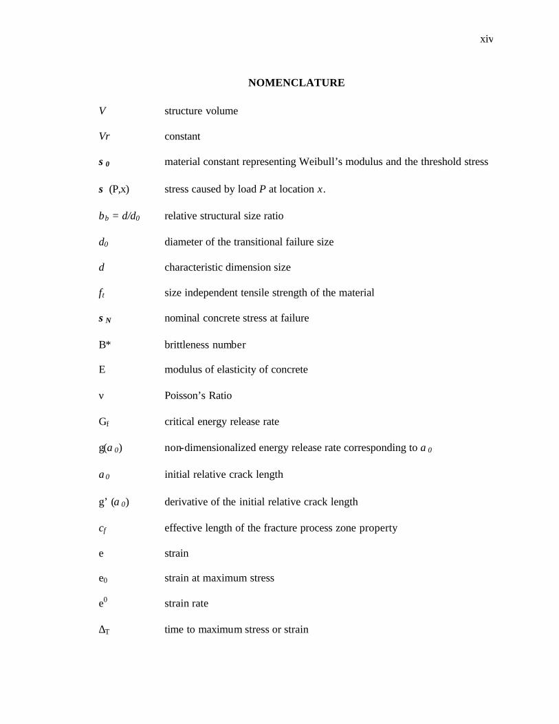
NOMENCLATURE
V structure volume
Vr constant
σ0 material constant representing Weibull’s modulus and the threshold stress
σ (P,x) stress caused by load P at location x.
βb = d/d0 relative structural size ratio
d0 diameter of the transitional failure size
d characteristic dimension size
ft size independent tensile strength of the material
σN nominal concrete stress at failure
B* brittleness number
E modulus of elasticity of concrete
ν Poisson’s Ratio
Gf critical energy release rate
g(α0) non-dimensionalized energy release rate corresponding to α0
α0 initial relative crack length
g’ (α0) derivative of the initial relative crack length
cf effective length of the fracture process zone property
e strain
e0 strain at maximum stress
e0 strain rate
∆T time to maximum stress or strain

xv
f’c concrete compressive strength
f’t concrete tensile strength
bw member width
d member effective depth
?w reinforcement ratio
av distance from the major load to the support
Mu factored moment
Vu factored shear force
Vc shear capacity of the member
ρ mass Density
dc material cohesion
β material angle of friction
R Cap eccentricity parameter in Drucker-Prager Cap Plasticity Model
α transition surface radius parameter Drucker-Prager Cap Plasticity Model
K ratio of flow stress
σc direct stress after cracking
ec direct cracking strain

xvi
ACKNOWLEDGMENTS
I would like to express my deep gratitude and profound thanks to my advisor, Dr.
Krauthammer, for all the help and support that he provided throughout all the stages of
this work. I would also like to thank the members of my committee, Dr. Schokker, Dr.
Koudela, and Dr. Varadan, for their valuable help.
I want to express my gratefulness to all the members of the Protective Technology Center
at Penn State University for their help and support. Special thanks are due to Mohammed
Zineddin, Stacy Worley, and Craig Starr for their help during the experimental phase.
The tests provided by the National Defense Academy in Japan under the supervision of
Dr. Ohno and Dr. Beppu and the tests performed at the University of British Colombia
under the supervision of Dr. Mindess were very essential for completing this work.
This study was sponsored by the National Science Foundation (NSF grant no. CMS-
9908344) and by the Norwegian Defence Construction Services support.
1
CHAPTER ONE
INTRODUCTION
1.1 Research Significance
Concrete structures have traditionally been designed on the basis of strength criteria.
This implies that geometrically similar structures of different sizes should fail at the same
nominal stress. However, this is not quite true in many cases because of the Size Effect,
which may be understood as the dependence of the concrete struc ture on its characteristic
dimension.
To civil engineers, the Size Effect is of paramount importance. Concrete structures are
designed based on the strength of a standard specimen size. The actual concrete strength
of relatively larger structural members may be significantly lower than that of the
standard size. By neglecting Size Effect, predicted load capacity values become
increasingly less conservative as a member size increases. Also, very large structures
such as dams, bridges, and foundations are too large and too strong to be tested at full
scale in the laboratory.
In recent years, major advances have been made in understanding of scaling and Size
Effect. However, these advances remain only in the static domain (i.e., slow loading
rates), and none of the previous studies have addressed the effect of higher loading rates
or high-strength concrete (HSC) on the Size Effect. Structural concrete can be subjected
to high loading rates, such as those associated with impact and explosion incidents. Such

2
load conditions are generated by dropped objects, vehicle collision into structures,
accidental industrial explosions, missile impacts, military explosions, etc.
The Size Effect in normal strength concrete (NSC) is a phenomenon explained by a
combination of plasticity and fracture mechanics, and it is related to the energy balance
during the damage/fracture process. Although structural response and damage evolution
are expected to be size-dependent, it is not clear how time or the material strength affect
this phenomenon.
1.2 Objective and Scope
The objective of this study is to assess the effect of time on the Size Effect for both
normal-strength concrete (NSC) and high-strength concrete (HSC) cylindrical specimens
under compressive severe dynamic loading conditions (loading rates of 10-3 sec). The
study was conducted by performing both static and dynamic tests and parallel numerical
simulations. The tests provided data whose analysis produced evidence on the effect of
loading rate and material strength on the Size Effect for structural concrete in
compression. Parallel pre- and post-test computational simulations were used to perform
‘numerical tests’ of the same structural/material specimens, and to explore the role of the
time dimension on the physical phenomena that contribute to the Size Effect. A
comparison between test and numerical data was done to assist and guide the investigator
in developing a better understanding of the Size Effect phenomenon (with emphasis on
short duration dynamics). In additions, the precision impact test data assisted in
validating the computational tools used for the study.

3
The dissertation describes the outcome of the experimental and numerical investigation,
and it presents data from both the impact tests and the related numerical simulations.
Discussions of the findings lead to conclusions and recommendations for future research
and possible implementation of these findings into the design of impact and blast
resistant structural concrete buildings and systems.
1.3 Thesis Layout
Chapter One of this thesis is an introduction that lists the scope and objective of the
thesis. Chapter Two is a background of the Size Effect phenomenon and the current state
of knowledge in this area. Chapter Three outlines the methodology of the study. Chapter
Four is a description of the test setup and the instrumentations used in the three different
test locations. Chapters Five and Six present the results of the tests and the simulations
for the high-strength and normal strength concrete cylinders respectively, theses chapters
also include a discussion of the results obtained. The results for the high-strength and
normal-strength concrete are compared in Chapter Seven, and conclusions and
recommendations for future work are given in Chapter Eight. Flow charts of work data
and samples of the results of the tests and the simulations are given in the Appendices.

4
CHAPTER TWO
LITERATURE REVIEW
2.1 Introduction
For a long time, it has been believed that the strength of concrete and concrete structures
is independent of the size. However, as a result of many studies that incorporated both
experimental and theoretical investigations, it has been verified that structural concrete
behavior (loaded in tension, compression, shear or torsion) is largely influenced by the
specimen size. The Size Effect was studied by behavioral comparisons of geometrically
similar test specimens. Initially, these observations were based on test data (Bazant and
Estenessoro 1979; Bazant and Planas 1998). However, later studies attempted to
correlate test data with various theoretical approaches and models (Hillerborg et al 1976;
Petresson 1981; Bazant and Oh 1984; Bazant 1997). It was shown in these studies that
larger compression specimens had steeper softening paths, and larger beams were weaker
in bending, shear and torsion. This phenomenon has been termed ‘Size Effect’. Various
explanations were proposed for those observations; for example, related to boundary
layer effects, due to differences in rates of diffusive phenomena, due to heat of hydration
or any other phenomena related to chemical reactions, due to a statistical fact based on
the number of defects in the volume, or related to energy dissipation during the evolution
of fracture and damage.
2.2 Classical Definition of Size Effect
Size effect may be understood as the dependence of the apparent strength of the concrete
element (more precisely, the nominal stress at failure) on its characteristic dimension.

5
This implies that geometrically similar structures of different sizes fail at different
nominal stresses. Size Effect can be defined through a comparison of geometrically
similar structures of different sizes, and is conveniently characterized in terms of the
nominal stress, σN, at maximum (ultimate) load, Pu. When the σN values for
geometrically similar structures of different sizes are the same, we say that there is no
Size Effect. A dependence of σN on the structure size (dimension) is called Size Effect.
2.3 Proposed Modification to the Definition of Size Effect
Since in this study, and in other studies, it was found that Size Effect is not only limited
to traditional and well established reduction in nominal strength with increases in size,
the author proposes a modification to the existing Size Effect definition to include all
these parameters that may not necessarily be related to the conditions at failure. The
modified definition is as follows:
Size Effect is the dependence of material properties (not necessarily at failure) on the
characteristic dimension of the structural element). It can be characterized in terms of the
the nominal stress at failure, the concrete modulus of elasticity, or the strain at maximum
stress. It can be understood through a comparison of geometrically similar structures of
different sizes.
2.4 Background
The early works on the Size Effect up until 1970’s relied primarily on extensive test
results, and there was no generally accepted theory for predicting the Size Effect.

6
Gonnerman (1925) conducted some of the earliest of studies on Size Effect in concrete.
He stated that, “Considerable data on the effect of specimen size and shape are available
for stone, masonry, piers, etc., but comparatively few tests have been carried out on
concrete; in the tests reported no attempt was made to differentiate between different
types of concrete”. He then conducted a series of experiments in which he tested the
compressive strength of cylinders of different sizes (1.5 inch (37.5 mm) to 10 inch (250
mm) diameters) with a height to diameter ratio of 2. He concluded that, for cylinders of
length equal to 2 times the diameter, lower strength values were generally obtained with
the larger cylinders. He also stated that the decrease in strength with the increase of
cylinder size was not important for diameters of 6 in. or less; 8 x 16 inch (200 x 400 mm)
and 10 x 20 inch (250 x 500 mm) cylinders gave 96 and 92 percent of the strength of 6 x
12 inch (150 x 300 mm) cylinders.
Other important tests followed, including (Bazant and Planas 1998) Humphreys 1957,
Rush et al. 1962, Kani 1967, Bhal 1968, McMullan and Daniel 1972, Taylor 1972,
Hillleborg et al. 1976, Walsh 1976, Walraven 1978,1990, Chana 1981, Peterson 1981,
Reinhardt 1981, Hankins 1985, Iguero et al. 1985, Hilleborge 1985,1989, Ingraffea 1985,
Rots 1988,1992 and others. As a result of all these studies, it has been established that
failure of concrete structures exhibit Size Effect.
After the 1970’s more rigorous theoretical basis for Size Effect have been established by
many investigators. The fictitious crack model by Hilleborg et al. (1976) and Petresson
(1981), the crack band model by Bazant and Oh (1984), and the notch sensitivity analysis

7
by Zaitsev and Kovler (1986), represent some of the attempts for a theoretical approach
to the Size Effect problem in concrete structures.
As a result of the previous studies, a model equation for prediction of the compressive
strength of plain concrete cylinders was proposed by Bazant (1989). The equation is
theoretically valid for geometrically similar concrete specimens, such as specimens with
fixed height to diameter ratio.
2.5 Evidence of Size Effect
The existence of Size Effect for concrete structures, subjected to static loading, has been
well established through many studies. Generally, this extensive and multifaceted
evidence can be divided into two major categories: experimental evidence and theoretical
evidence.
2.5.1 Theoretical Evidence
Theoretically, the existence of Size Effect has been verified by many different
approaches such as:
a) Analytical solution of energy release and localization of instabilities for various
simplified situations (ACI Committee 446 1992; Bazant and Planas 1998).
b) Dimensional analysis and similitude arguments (Bazant and Planas 1998).
c) Numerical micro structural simulation on a super computer in which concrete was
modeled as a random array of particles (hard aggregate pieces) with a softening inter-
particle force-displacement relation (Van Meir 1985; Bazant and Ozbolt 1990).

8
d) Non-linear fracture mechanics solutions based on the fictitious crack model with a
gradually softening law for the crack bridging stress (Hillerborg et al. 1976; Ma,
Niwa, and McCabe 1992). Zareen and Niwa (1994) performed similar fictitious
crack analysis. Their results showed conclusively that a Size Effect existed for shear
critical beams.
e) Deterministic limit of a non- local generalization of Weibull–type statistical strength
theory (Bazant and Xi 1991).
f) Finite element solution based on the smeared crack approach (Bazant and Oh 1983;
Bazant and Lin 1988; Rots 1994; Eligehausen and Ozbalt 1990; Cervenka and Pukl
1994) and discrete crack approach (Ingraffea 1985; Bocca, Carpinteri, and Valente
1990). Gustafsson and Hillerborg (1988) used the finite element method to model
Size Effects due to discrete cohesive diagonal tension in singly reinforced beams
without shear reinforcement. They found a significant fracture mechanics Size
Effect. Ozbolt and Eligehausen (1991) studied the Size Effect on shear resistance of
reinforced concrete beams using a non local micro-plane model and plane stress finite
elements. The calculated results demonstrated a decrease in average strength with an
increase in member size. Kotsovos and Pavlovic (1997) used three-dimensional finite
element analysis on reinforced concrete beams with and without stirrups. They
proved the existence of Size Effect in beams.

9
2.5.2 Experimental evidence
The available experimental evidence for the existence of Size Effect in the static domain
is extensive and multifaceted and covers most of the various types of failures of structural
concrete as detailed below:
2.5.2.1 Size Effect in Concrete Compressive Strength
The effect of size on concrete compressive strength has been proved through many
studies and for different types of specimens with variable dimensions and ratios (as long
as geometric similarity is maintained). Many studies, such as those performed by Harris
et al. (1963), Sabnis, Pahl and Soosar, Baalbaki et al (1992), Lessard et al. (1993), Aïticin
et al. (1994), and Sener (1997), examined the variation of concrete compressive strength
with age and volume for concrete cylinders of different sizes. The results showed that
small specimens exhibited higher compressive strength values than the larger ones.
Neville (1996) proved the existence of Size Effects on compressive strength of concrete
cubes of different volumes.
Marti (1989) reported the existence of Size Effect in double-punch compression failure of
cylinders.
2.5.2.2 Size Effect in Concrete Tensile Strength
Harris et al (1963) and Mirza (1992) conducted tests to determine if size affects the
measured tensile strength of concrete. Large Size Effects in both the modulus of rupture
and the split cylinder tests were observed. Harris et al (1963) suggested that like
compressive strength, tensile strength is affected by method of loading, specimen size,

10
concrete mix properties, method of casting, workmanship, differential drying, strain
gradient, and volume effects. Brazilian split cylinder tests were also found to be affected
by the specimen size (Bazant et al. 1991).
2.5.2.3 Size Effect in Strain Gradient and Cracking Strain
Chana (1985) conducted a series of tests on concrete prisms of the same size but
subjected to different combinations of axial, eccentric and flexural loads, giving different
strain gradients. He concluded that an increase in modulus of rupture with decreasing
depth and the onset of cracking in model beams can partly be attributed to a strain
gradient effect. As the depth of the member decreases, the strain gradient increases,
resulting in a higher cracking strain.
2.5.2.4 Size Effect in Ultimate Shear Strength
Chana (1985) reported a decrease in shear strength with the increase of specimen size.
He also observed that the residual shear strength of post-cracking shear strength defined
as the difference between the ultimate loads and the first cracking load is almost constant
irrespective of scale.
2.5.2.5 Size Effect in Diagonal Shear Failure of Beams without Stirrups
The existence of Size Effect in the diagonal shear failure of longitudinally reinforced
concrete beams with or without stirrups, prestressed or unprestressed was observed by
Bazant and Kim (1984), Bazant and Sun (1987), and Bazant and Kazemi (1991). The
latter conducted experiments on a wide range of sizes ratios up to 1:16, they stated that
the observed Size Effect was weaker for beams with longitudinal bars not provided with
hooks at the ends in order to prevent bar pull-out.

11
2.5.2.6 Torsional failure
Bazant et al (1988) proved that torsional failure of longitudinally reinforced beams
without stirrups and non-reinforced beams exhibits Size Effect.
2.5.2.7 Punching shear failure of slabs
Bazant and Cao (1987) showed the existence of Size Effect in punching shear failure of
slabs with a one-side reinforcement mesh
2.5.2.8 Pull-out failures
The existence of Size Effect was observed for pull-out failure of deformed reinforcing
bars (Bazant and Sener 1988), pull-out failure of headed anchors, with a conical failure
surface and different embedment depths (Eligehausen and Swade 1989), and bond splices
(Sener 1992)
2.5.2.9 Compression failure of tied columns
Compression failure of tied columns, short as well as slender, was found to be influenced
by size (Bazant and Kwon 1994).
2.5.2.10 Three-point bending of beams
Study by Ozbolt, Eligehausen, and Petrangeli (1994) found that three-point bending of
beams and uniform loading of reinforced/non-reinforced and notched/un-notched beams
were prone to Size Effects.

12
2.5.2.11 Influence of Specimen Size on Elastic Modulus of Concrete
The effect of specimen size on elastic modulus has not been well researched. Tests
conducted by Baalbaki et al. (1992), on 100×200 mm and 150×300 mm specimens of
high performance concrete resulted in the 100 mm samples exhibiting higher
compressive strengths and the 150 mm samples exhibiting higher modulus of elasticity.
The resulted higher strength in the smaller specimens is inline with the results of other
researchers, but the increased stiffness as specimen size increases is an interesting result.
2.6 Explanation of Size Effect
For a long time, Size Effect has been explained statistically as a consequence of the
randomness of material strength, particularly by the fact that in a large structure it is more
likely to encounter a material point of smaller strength. Various existing test data were
interpreted in terms of Weibull’s weakest link theory. However it was proposed that
whenever the failure does not occur at the initiation of cracking, which represent the most
situations for concrete structures, the Size Effect should properly be explained by energy
release caused by macro crack growth, and that the randomness of strength plays only a
negligible role (Bazant and Xi 1991).
2.6.1 Statistical Theory
Statistical Size Effect, which is caused by the randomness of material strength, has
traditionally been believed to explain most Size Effects in concrete structures. This
theory of Size Effect, originated by Weibull (1939), is based on the model of a chain.
The failure load of a chain is determined by the minimum value of the strength of the

13
links in the chain, and the statistical Size Effect is due to the fact that the longer the chain,
the smaller is the strength value that is likely to be encountered in the chain. This
explanation, which certainly applies to the Size Effect observed in the failure of a long
concrete bar under tension, is described by Weibull’s weakest link statistics.
The probability of failure of a concrete structure and the mean nominal stress at failure
can be obtained by using Weibull-type theory as follows;
−−= ∫
V r
m
VxdVxP
Pob)(),(
exp1)(Pr0σ
σ (2.1)
[ ]∫∞
−=0
)(Pr11
dpPobbdNσ (2.2)
where V is the volume of the structure, Vr is a constant, m and σ0 is a material constant
representing the Weibull modulus and the threshold stress, and σ (P,x) is the stress
caused by load P at location x.
If the structures fail at initiation of macroscopic crack growth-which is the case for most
metallic structures, or long uniformly stressed bars, the stress distribution is calculated
according to elasticity for a structure without any crack.
However, on close scrutiny this explanation is found to be inapplicable to most types of
failures of reinforced concrete structures (Bazant and Planas 1998). In contrast to
metallic and other structures, which fail at the initiation of a macroscopic crack (i.e. as
soon as a microscopic flaw or crack reaches macroscopic dimensions), concrete

14
structures fail only after a large stable growth of cracking zones or fractures. The stable
crack growth causes large stress redistributions and a release of stored energy, which in
turn, causes a much stronger Size Effect. The stress values farther away from the tip of a
macro-crack are relatively small and make a negligible contribution compared to the
stresses in the volume of the fracture process zone around the macro-crack tip. i.e., the
volume in which the strength values matter is quite small—usually a small part of the
entire volume of the structure. This causes the random strength values outside this zone
to become irrelevant, thus suppressing the statistical Size Effect. This implies strongly
that another explanation other than the statistical theory should be used to describe the
Size Effect. It was also shown that some recent experiments on diagonal shear failure of
reinforced concrete beams contradicted the predictions of the statistical theory (Bazant
and Planas 1998).
2.6.2 Energy Theory and the Size Effect Law
This is the most important source of Size Effect; it is also know as the fracture mechanics
Size Effect. It is caused by the release of stored energy of the structure into the fracture
front and the transition of the failure mode from plasticity to fracture mechanics.
The failure stress of a series of geometrically similar structures of different sizes can be
expressed by the following infinite series (Bazant 1986):
σNc = Bft [βb + 1 + L1βb-1 + L2βb-2 + …]-1/2 (2.3)
In which B, d0, L1, L2, etc. are constants, βb = d/d0 is the relative structural size ratio, and
ft is the size independent tensile strength of the material under consideration. Equation
(2.3) represents an asymptotic expansion of the failure stress for a geometrically similar

15
structure with respect to the relative structure size. Also, it was shown that for the size
range up to βb = 1/20, the asymptotic series can be truncated after the linear term
resulting in the Size Effect law (Bazant and Planas 1998):
0
1dd
Bf tNc
+=σ (2.4)
Figure 2.1 shows the relationship of the nominal stress at failure σN and characteristic
dimension size d, provided that the cracks at the moment of failure of geometrically
similar structures of different sizes are also similar.
Figure 2.1 Size Effect Law
A simple expression was proposed by Bache (1993) for describing the brittleness of the
structure in terms of a brittleness number, B*:
EGDf
Bf
t2
* = (2.5)

16
In which ft and d were defined earlier, E is the modulus of elasticity of concrete, and Gf
is the critical energy release rate. It can be seen from Equation (2.5) that the brittleness
increases as the depth of the structure (D) increases, resulting in lower strength.
Those relationships can be most simply explained by considering uniformly stressed
rectangular panels of different sizes d, loaded by uniformly distributed load σN as shown
Figure 2.2, and by setting some assumptions.
Figure 2.2 Explanation of Size Effect Due to Stored Energy Release From the Cross Hatched Areas (ACI Committee 446 1992)

17
Those assumptions are (1) the propagation of a fracture or crack band requires an
approximately constant energy supply per unit length and width of fracture, (2) the
potential energy released by fracture from the structure is a function of both the length of
fracture and the area of the cracking zone (fracture process zone) at the fracture front, (3)
The failure modes (i. e., fracture shapes and lengths) of geometrically similar structures
of different sizes are, at the moment of maximum load, also geometrically similar, and
(4) the structure does not fail at crack initiation.
When the fracture extends by ∆a, the additional strain energy that is released into the
fracture front comes from the densely cross-hatched strip of horizontal dimension ∆a.
Because the area related with strain energy release is ha + ka2, the incremental area by the
incremental ∆a is
h(a+∆a) + k(a + ∆a)2 - (ha + ka2) = h∆a + 2ka∆a + k(∆a)2
This reduces to h∆a +2ka∆a, because (∆a)2 can be neglected, where k—the slope in
Figure 2.2—forms an empirical constant depending on the structure shape.
The strain energy released from the aforementioned densely cross-hatched strip is
∆W= b (h∆a+ 2ka∆a) σN2/2E, where b is the panel thickness. Setting ∆W=Gf b∆a, the
dissipated energy, we can obtain σN 2[h+2k(a/d)d] =2EGf.
Solving for σN, we can bring the resulting expression to the form of the Size Effect law
σN =Bf’t (1+β)-1/2 , β=d/d0 (2.6)
in which B=(2EGf / hf’t2)1/2, d0=hd/2ka, and f’t is the direct tensile strength of concrete.

18
For small enough structures (compared to d0), i. e., d<<d0 Equation 2.6 yields a constant,
which means the Size Effect disappears. The plastic limit analysis or elastic allowable
stress design is then valid. This has been the case for most laboratory tests so far. For d
>> d0 the fracture process zone size is negligible compared to the structure size, which is
the case of linear elastic fracture mechanics. Equation 2.6 reduces in this case to
σN = Bf’tβ -1/2 or log σN = -1/2 log d + const. (2.7)
The intersection point of the above two asymptotes is obtained by setting Bf’t = Bf’t β -1/2 ,
which yields β = 1 or d = d0.
The transitional Size Effect curve shown in Fig 2.1 can also be obtained by numerical
models of the microstructure, such as the random particle model or non- local finite
models in which localization of cracking is restricted to a zone of a certain minimum size.
Equation 2.6 can be used to determine the fracture energy and the effective length of the
fracture process zone which characterize the nonlinear fracture.
f
t
EGf
agB2'
02 )(=β (2.8)
fcgdg
)()(
0'
0
αα
β = (2.9)
where g(α0) is the non-dimensionalized energy release rate corresponding to the initial
relative crack length α0 = a0 d; according to linear elastic fracture mechanics, g’ (α0) is its
derivative, and cf is the effective length of the fracture process zone, which is a material
property.
19
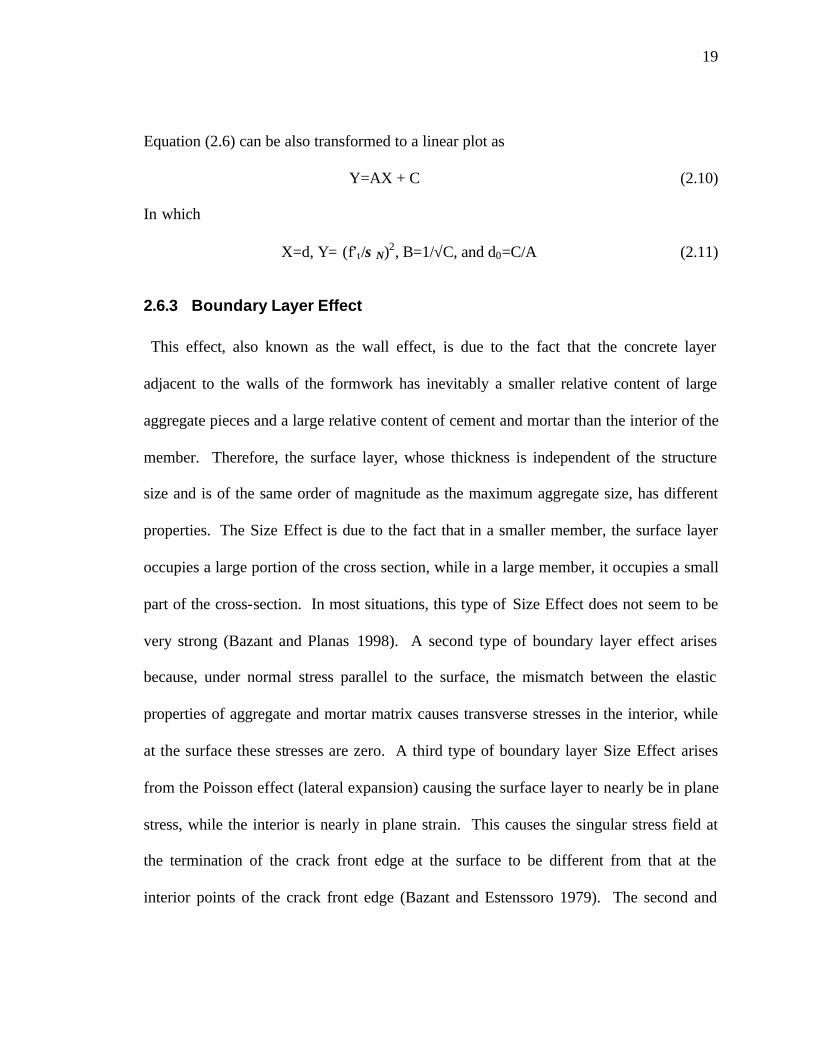
Equation (2.6) can be also transformed to a linear plot as
Y=AX + C (2.10)
In which
X=d, Y= (f’t/σN)2, B=1/√C, and d0=C/A (2.11)
2.6.3 Boundary Layer Effect
This effect, also known as the wall effect, is due to the fact that the concrete layer
adjacent to the walls of the formwork has inevitably a smaller relative content of large
aggregate pieces and a large relative content of cement and mortar than the interior of the
member. Therefore, the surface layer, whose thickness is independent of the structure
size and is of the same order of magnitude as the maximum aggregate size, has different
properties. The Size Effect is due to the fact that in a smaller member, the surface layer
occupies a large portion of the cross section, while in a large member, it occupies a small
part of the cross-section. In most situations, this type of Size Effect does not seem to be
very strong (Bazant and Planas 1998). A second type of boundary layer effect arises
because, under normal stress parallel to the surface, the mismatch between the elastic
properties of aggregate and mortar matrix causes transverse stresses in the interior, while
at the surface these stresses are zero. A third type of boundary layer Size Effect arises
from the Poisson effect (lateral expansion) causing the surface layer to nearly be in plane
stress, while the interior is nearly in plane strain. This causes the singular stress field at
the termination of the crack front edge at the surface to be different from that at the
interior points of the crack front edge (Bazant and Estenssoro 1979). The second and

20
third types exist even if the composition of the boundary layer and the interior layer is the
same.
2.6.4 Diffusion Phenomena
Diffusion phenomena, such as heat conduction or pore water transfer (curing rate), are
contributors to the Size Effect phenomenon. Their Size Effect is due to the fact that the
diffusion half- times (i.e., half times of cooling, heating, drying, etc.) are proportional to
the square of the size of the structure. At the same time, the diffusion process changes
the material properties and produces residual stresses, which in turn produce inelastic
strains and cracking. For example, drying may produce tensile cracking in the surface
layer of the concrete member. Due to different drying times and different stored
energies, the extent and density of cracking may be rather different in small and large
members, thus engendering a different response. For long time failures, it is important
that drying causes a change in concrete creep properties, that creep relaxes these stresses
and that in thick members the drying happens much slower than in thin members.
Aïticin et al. (1994) investigated the effect of cylinder size and curing on the measured
compressive strength of different strength high-strength (HS) concretes. The research
involved testing 5000, 13,000, and 17,500 psi (34.5, 89.7, and 120.7 MPa) concrete in
compression with 4, 6, and 8 inch (100, 150 and 200 mm) diameter cylinders.
Compressive strengths for three specimens of each size were tested after 1, 7, 28, 91, and
365 days. The results of these tests showed the effect of cylinder size on the compressive
strength of concrete. For the 5000 and 13,000 psi concrete, the compressive strengths of
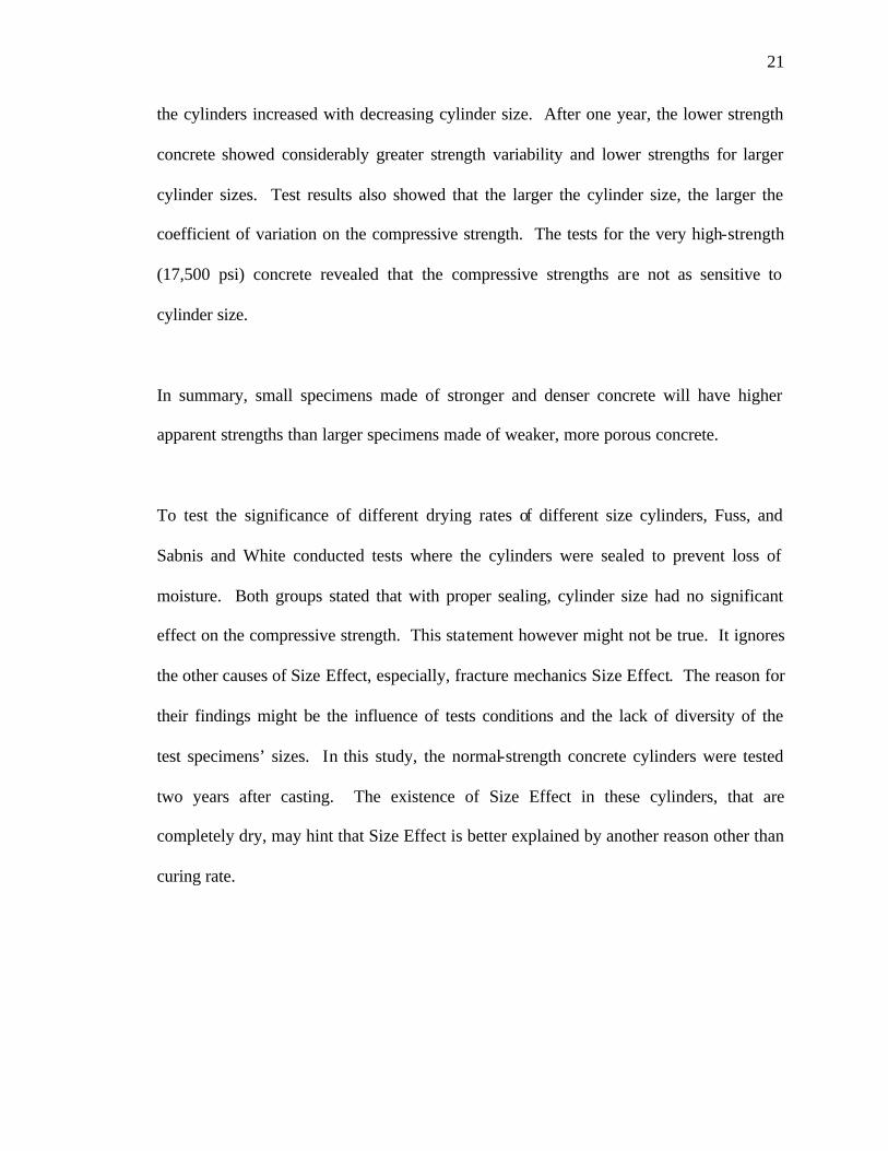
21
the cylinders increased with decreasing cylinder size. After one year, the lower strength
concrete showed considerably greater strength variability and lower strengths for larger
cylinder sizes. Test results also showed that the larger the cylinder size, the larger the
coefficient of variation on the compressive strength. The tests for the very high-strength
(17,500 psi) concrete revealed that the compressive strengths are not as sensitive to
cylinder size.
In summary, small specimens made of stronger and denser concrete will have higher
apparent strengths than larger specimens made of weaker, more porous concrete.
To test the significance of different drying rates of different size cylinders, Fuss, and
Sabnis and White conducted tests where the cylinders were sealed to prevent loss of
moisture. Both groups stated that with proper sealing, cylinder size had no significant
effect on the compressive strength. This statement however might not be true. It ignores
the other causes of Size Effect, especially, fracture mechanics Size Effect. The reason for
their findings might be the influence of tests conditions and the lack of diversity of the
test specimens’ sizes. In this study, the normal-strength concrete cylinders were tested
two years after casting. The existence of Size Effect in these cylinders, that are
completely dry, may hint that Size Effect is better explained by another reason other than
curing rate.

22
2.6.5 Hydration Heat or Other Phenomena Associated With Chemical
Reactions
This effect is related to the diffusion in that the half-time of dissipation of the hydration
heat is produced in a concrete member is proportional to the square of the thickness (size)
of the member. Therefore, thicker members heat to higher temperatures, a well-known
problem in concrete construction. Again, the non-uniform temperature rise may cause
cracking, induce drying, and significantly alter the material properties.
2.6.6 Influence of aggregate size on Size Effect
The fracture parameters as well as the Size Effect law are valid only for structures made
of the same concrete, which implies the same aggregate size. If the aggregate size is
changed, the fracture parameters and the Size Effect law parameters change.
Saouma (1994) reported that the aggregate size does not seem to affect the Size Effect of
nominal strength concrete, but the shape and geological composition of aggregates should
be of more importance.
Johnson (1962) studied the effect of scaling the aggregates for concrete mixes suitable for
models of concrete structures using high early strength cement, natural sand, and four
different maximum size aggregates. He used ¾ inch (19 mm) aggregate for prototype
concrete, 3/16 inch (4.8 mm) for ¼-scale model concrete, and 3/32 inch (2.4 mm) for 1/8-
scale concrete. Cubes and cylindrical specimens were used for each test series. He found
that the 6 in. diameter cylinders were about 75-85% as strong as the 1.5 in. diameter
cylinders for both the ¼ and 1/8 scale mixes.

23
Although the above results hint that the aggregate size have no influence in the Size
Effect phenomenon, more research need to done before a final conclusion can be made.
2.7 Size Effect in High-Strength Concrete (HSC)
Lessard, et al. (1993) investigated the influence of different parameters related to testing
HSC, involving 14 different concretes and 378 specimens, he found that f’c for a 100 mm
cylinder is 1.05 times f’c for a 150 mm cylinder. Hence he concluded that the
compressive strength of high-strength concrete (HSC) depends on the specimen size.
Similar results were obtained by Baalbaki et al. (1992).
Testing on high strength concrete by Eo (1994) suggested that Bazant’s Size Effect law
was not as effective in predicting the nominal strength as the following formula, in which
B, d0, and α are constants that can be obtained from regression analysis of experimental
data (Eo, Hankins, and Kono 1994):
σN = (Bft) / [(1+d/d0)1/2] + α *ft (2.12)
Eo claims that this formula is more accurate due to the fact that the limiting value in the
nominal strength, as beam size increases, is achieved more rapidly when high strength
concrete is used.
Zhou et al. (1998) conducted experiments on normal and light weight high-strength
concrete. They reported that Bazant’s Size Effect law gave a very good account of the
Size Effect on flexural strength for both types of concrete. However, the torsional
strength of the light weight high-strength concrete appeared to have a stronger size
24
dependency than the normal weight HSC. They also observed a reverse Size Effect in the
tensile strength of both the normal and the light weight HSC.
2.8 Size Effect in the Dynamic Domain
The concept of Size Effects has not been studied extensively in the dynamic domain, and
its form under short duration dynamic (e.g., blast or impact) loading conditions is not
known. Nevertheless, some available data show a relationship between loading rate
(time to peak load varied between 1.4 s and 253,000 s) and Size Effect (Lessard et al.
1993). They showed that Equation (2.4) can be used to relate the loading rate with
fracture mechanics parameters (e.g., crack mouth opening displacement, load-point
displacement, etc.), and that the corresponding functions exhibit a clear rate effect. That
study showed the following:
• The Size Effect model agrees with test results for the loading rates given above.
• A decrease in loading rate resulted in a higher brittleness and a closer correspondence
to linear elastic fracture mechanics (LEFM).
• The fracture toughness, effective fracture process zone length, and effective critical
crack tip opening displacement (CTOD) all decreased with a slower load rate.
These observations showed that creep in concrete is strongly related to fracture. Creep
studies (Aïticin et al. 1994) with loading rates between 0.05X10⁻⁶ m/s and 50X10-6 m/s
showed clear relationships between loading rates and fracture mechanics properties (time
to peak load, fracture energy, etc.). The loading rates employed previously, however, are
very slow for practical short duration dynamic processes, where the rise time could be on

25
the order of 1X10⁻³ seconds. Obviously, those studies are not sufficient to determine a
Size Effect relationship for severe dynamic loading conditions, such as those obtained
from impact or explosions.
2.9 Design and Code Issues
Consideration of Size Effect in design regulations is underaddressed, if even recognized
in many building codes. The CEB/FIP Model Code of 1990 has taken the greatest strides
to incorporate Size Effect findings into rational design methods by taking specific
consideration for the softening behavior induced by cracking through introducing values
for fracture properties and specific size factors for shear failure. Many European codes,
including the Eurocode and codes used in the Netherlands, Germany, Norway, Sweden
and England include a similar shear failure size factors, as does the Japanese code.
However, the ACI Code, along with the Swiss, Canadian, and Danish codes, does not
address this issue at all (Walraven 1994).
Arguments for the replacement of current empirical shear design methods found in the
ACI Code with theoretically-based methods have been based upon the obvious visible
nature of the Size Effect relationships. However, steps to incorporate this into the ACI
Code have yet to be taken, and by neglecting the Size Effect, predicted load capacity
values become increasingly less conservative as a member size increases. It has been
suggested that the reluctance of many engineers to include Size Effect factors in the ACI
Code is based upon a fear of the incorporation of complicated fracture mechanics into
simpler design methods (McCabe and Niwa 1994).

26
McCabe and Niwa (1994) performed a finite element analysis comparative study on the
existing ACI design equations for shear versus the equations found in the Japanese
(JSCE) and European (CEB) codes which incorporate Size Effect considerations. In
order to perform this analysis, the finite element mesh assumed that failures occurred
from flexural shear cracks inclined at 26° from the horizontal, and located a distance d
from the end of the beam. The following are the equations compared:
Vc = f’c0.5 * bwd / 6.0 and Vc = [(f’c
0.5 + 120ρw (Vud / Mu)) / 7.0] bwd (ACI 318)
Vc = [0.19 (100ρwf’c)1/3 d-1/4] bwd (JSCE)
Vc = {0.15(3d/av)1/3 (100ρwf’c)1/3 [1+(0.2/d)1/2]} bwd (CEB-FIP)
where Vc is the shear capacity, f’c is the concrete strength in MPa, bw is the member
width, d is the effective depth, ?w is the reinforcement ratio, av is the distance from the
major load to the support, and Vu and Mu are the factored shear and moment,
respectively.
They found that the Japanese and CEB-FIP codes closely approximated the data acquired
in the analysis. This was expected due to the fact that the equations in these codes take
into account Size Effect. The failure of the ACI code values to approximate this data
revealed that the Code tends to overestimate the shear strength of large-sized beams, and
the ACI’s negligence of the Size Effect phenomena is indeed consequential. At a depth
greater than 300 mm the ACI equations overestimate nominal shear strength.
Incorporation of the Size Effect into shear design equations in a manner similar to the

27
CEB-FIP code and the Japanese code could provide more accurate approximations of
shear behavior (McCabe and Niwa 1994).
2.10 Summary of Key Issues for this Study
1 Study of Size Effect in the dynamic domain.
2 Loading rate effect and the way it interacts with Size Effect.
3 How the Size Effect Law behaves with HSC cylinders.
4 Does Size Effect exist in parameters other than strength such as the modulus of
elasticity and the stain at maximum stress?
5 Changes in the modes of failure.

28
CHAPTER THREE
METHODOLOGY This study comprised a combined testing and numerical simulations efforts aimed at
enhancing the understanding of the possible effect of compressive impact loads on the
Size Effect phenomenon. The testing activities on normal and high-strength concrete
cylinders focused on collecting test data whose analysis could provide evidence on the
effect of impact loads on the Size Effect phenomenon for both normal and high-strength
structural concrete under axial compressive loads.
The numerical simulations involved two parts, pre-test and post-test simulations. The
pre-test simulations were carried out first, using preliminary information about the test
setup and the materials to be used. The results from the pre-test simulations were then
used to assess what could happen in the tests, and the range of parameters and their
locations. The impact tests were performed in three laboratories, following the pre-test
simulation stage. The third step was to study the test data and compare it with the pre-
test numerical simulations. Then, as needed, the numerical models were modified in an
attempt to match more accurately the test settings and related parameters (e.g. various
material properties, hammer-specimen interface conditions, steel transfer plate geometry,
impact velocities, etc). The results from the post-test simulations were then used for
additional comparison with the test results and the theoretical models.

29
3.1 Pre-test Simulations
Finite element simulations were carried out before the experimental work in order to aid
in test setup, planning, and other preparations for extracting data for the parameters that
would be measured in the tests. The pre-test simulations helped in assessing the
anticipated behavior and in designing the tests.
The finite element pre-test simulations were performed using the finite element code
ABAQUS Explicit (version 5.8). The structural models were made in such a way that
they represented the various specimen geometries and a general test setup. Two
constitutive models were used to model concrete properties, a plasticity-based model and
a fracture-based model. For each type of concrete, four different sizes of concrete
cylinders were modeled. The cylinder sizes for both the study on normal strength
concrete and the study on high-strength concrete are identical, the only difference is that
the high-strength concrete cylinders were all manufactured and tested in metric units,
while the normal-strength concrete cylinders were all manufactured and tested in English
units.
For the high-strength concrete study, the following cylinder sizes were used (as shown in
Figure 3.1):
• 75 mm x 150 mm,
• 150 mm x 300 mm,
• 300 mm x 600 mm, and
• 600 mm x 1200 mm

30
600 mm
120
0 m
m
300 mm
600
mm 150 mm
300
mm
150
mm
75 mm
Figure 3.1 High Strength Concrete Specimens Sizes
Each of the four high strength concrete (HSC) cylinder sizes was modeled eight times, as
follows: Using the two concrete models, with and without strain rate effects, and for two
different drop speeds, (10 m/s and 5 m/s).
For the normal-strength concrete study, the following cylinder sizes were used (as shown
in Figure 3.2):
• 3 inch x 6 inch
• 6 inch x 12 inch
• 12 inch x 24 inch
• 24 inch x 48 inch

31
24 inch
48 in
ch
12 inch
24 in
ch 6 inch
12 in
ch
6 in
ch
3 inch
Figure 3.2 Normal Strength Concrete Specimens Sizes
Each of the four normal strength concrete (NSC) cylinder sizes was modeled twelve
times using three different drop speeds (1 m/s, 5 m/s, and 10 m/s) instead of two as used
for the high-strength concrete (HSC). Fifteen control (sampling) elements were used for
the analysis, as shown in Figure 3.3. These elements were located at five different
elevations distributed along the depth of each cylinder. Each surface had three elements
located on a straight line that connected the center of the cylinder cross-section to the
edge of the cross section. The first element was at the centre of the cylinder; the last
element was at the edge of the cylinder, while the second element was midway between

32
the other two. The curves of stress vs. time, and strain vs. time were extracted for each
one of these 15 elements. This was done for each one of the 128 different simulations.
Figure 3.3 Distribution of Control Elements in the Simulated Cylinders
The element type used for modeling the concrete cylinders was an 8-node brick element
(element type C3DR8 in ABAQUS), as shown in Figure 3.3. The material models used
for concrete were the Drucker-Prager Cap Plasticity model, and the Brittle Fracture
concrete model. Each one of these models was used twice; first without including strain
rate effects for concrete; and second with strain rate effects included.
3.1.1 Description of the Concrete Constitutive Models
a) The Modified Drucker-Prager Plasticity Model
This model is based on a modified Drucker-Prager plasticity model. The *CAP
PLASTICITY option was used to define the yield surface parameters. The addition of
the Cap yield surface to the Drucker-Prager model serves two main purposes: it bounds

33
the yield surface in hydrostatic compression, thus providing an inelastic hardening
mechanism to represent plastic compaction; and it helps to control the volume dilatation
when the material yields in shear by providing softening as a function of the inelastic
volume increase created as the material yields on the Drucker-Prager shear failure
surface.
The yield surface has two principal segments: a pressure-dependent Drucker-Prager shear
failure segment and a compression cap segment as shown in Figure (3.4). The Drucker-
Prager failure segment is a perfectly plastic yield surface (no hardening). Plastic flow on
this segment produces inelastic volume increase (dilatation) that causes the cap to soften.
On the cap surface the plastic flow causes the material to compact.
Figure 3.4 The Modified Drucker-Prager Cap Plasticity Model

34
Some of the important input data for the Drucker-Prager model are: concrete compressive
strength, and the materials cohesion, dc. The Druckr-Prager failure surface is written as
Fs = q– p tanβ - dc = 0 (3.1)
Where β is the material’s angle of friction and R is a material parameter that controls the
shape of the cap. α is a small number (typically 0.01 to 0.05) that is used to define a
smooth transition surface between the shear failure surface and the cap. K is a material
parameter that may depend on temperature. Table (3.1) lists the input parameters for the
Drucker-Prager Cap plasticity model.
Table 3.1 Input Parameters used for the Pre-Test Drucker-Prager Plasticity Model
Concrete Compressive Strength, f’c 4,000 psi (NSC) / 14500 psi (HSC)
Mass Density, ρ 2.6x10⁻³ lb.sec2/in4
Poisson’s Ratio, ν 0.2
Young’s Elastic Modulus, E 3.6x10⁶ psi (NSC) / 6.86x10⁶ psi (HSC)
Material Cohesion, dc 400 psi (NSC) / 1450 psi (HSC)
Material Angle of Friction, β 51
Cap Eccentricity Parameter, R 0.65
Initial Cap Yield Surface Position 1.1x10⁻³
Transition Surface Radius Parameter, α 0.6
Ratio of Flow Stress, K 1.0
Strain Rate Effect factor 1.5

35
The Brittle Fracture Model
The Brittle Fracture Model in ABAQUS EXPLICIT provides capability for modeling
concrete in all types of structures; it can also be useful for modeling other brittle
materials such as ceramics or brittle rocks which behavior is dominated by tensile
cracking.
ABAQUS EXPLICIT uses a smeared crack model to represent the discontinuous brittle
behavior in concrete. It does not track individual macro cracks; instead constitutive
calculations are performed independently at each material point of the finite element
model. The presence of cracks enters in these calculations by the way in which the
cracks affect the stress and material stiffness associated with the material point. The
model assumes fixed orthogonal cracks with the maximum number of cracks at a material
point limited by the number of direct stress components present at that material point in
the finite element model. A simple Rankine criterion is used to detect crack initiation.
This criterion states that a crack forms when the maximum principal tensile stress
exceeds the tensile strength of the brittle material. Although crack detection is based
purely on Mode I fracture considerations, ensuing of the cracked behavior includes both
Mode I (tension softening/stiffening) and Mode II (shear softening/retention) behavior.
The Brittle Fracture Model assumes that the material is linear elastic in compression till
cracking occurs. The post cracking behavior is governed by a post failure stress that is
represented as a function of strain across the crack using the *BRITTLE CRACKING,
TYPE=STRAIN option (Figure 3.5)

36
Figure 3.5 The Brittle Fracture Model
Some of the important input data for the Brittle Fracture model are: the remaining direct
stress after cracking σc, and the direct cracking strain ec. The Druckr-Prager failure
surface is written as
Table (3.2) lists the input parameters for the Brittle Fracture model.
Table 3.2 Input Parameters used for the Pre-Test Brittle Fracture Model
Concrete Compressive Strength, f’c 4,000 psi (NSC) / 14500 psi (HSC)
Mass Density, ρ 2.6x10⁻³ lb.sec2/in4
Poisson’s Ratio, ν 0.2
Young’s Elastic Modulus, E 3.6x10⁶ psi (NSC) / 6.86x10⁶ psi (HSC)
Remaining Direct Stress After Cracking, σc 400 psi (NSC) / 1450 psi (HSC)
Direct Cracking Strain, ec 51
Strain Rate Effect factor 1.5

37
3.2 Tests
Impact tests were carried out on normal and high-strength concrete specimens under
impact velocities of 5 m/s and 7 m/s. The 10 m/s velocity could not be achieved during
the tests, and the 1 m/s was found to be not enough to break the large cylinders, so the 7
m/s was used instead. Details of the testing activities were as follows:
3.2.1 Tests on Normal-Strength Concrete (NSC) Cylinders
The study on normal strength concrete comprised both soft impact (using a rubber pad on
top of the concrete cylinder) and hard impact (without using a rubber pad on top of the
concrete cylinder). The selected normal concrete was designed to achieve a uniaxial
strength of 4,000 psi (27.6 MPa). All concrete specimens were made at the same time, by
the same manufacturer (The University of British Colombia, UBC), from the same mix.
Static tests were performed on the three small cylinder sizes, no machine was found with
enough capacity to test the big cylinder size. The results of the static tests will be
presented in the result chapter and will be compared with the static Size Effect law, and
with the dynamic results. The main dynamic tests on the normal-strength concrete
cylinders were conducted at Penn State University (PSU) with parallel validation tests at
the University of British Colombia (UBC) in Canada, and the National Defense Academy
(NDA) in Japan. The validation tests provided a means of comparison between the
results obtained at Penn State University and the results obtained by the smaller drop
hammer at (UBC) and a comparable drop hammer at (NDA). The number of impact tests
performed is as follows:

38
Number of tests = M sizes X N drop velocities X O interface conditions X P tests per
combination
The details of testing activities carried are presented next,
1. Tests at Penn State University (PSU): Theses were the main tests for the NSC using
the PSU drop hammer with its up to 29 kN (6500 lbs) weight. The tests at the UBC
and the NDA were conducted to insure the data objectivity by validating the test data
from PSU, and to establish a comparison between the data obtained at different
facilities.
Initially, it was proposed that tests at Penn State would be conducted on all the four
specimen sizes (3 x 6 inch, 6 x 12 inch, 12 x 24 inch, and 24 x 48 inch), however, during
preparations for the tests, and after testing many calibration cylinders, it was discovered
that testing the small cylinder size at Penn State would not yield good results, since the
weight of the hammer and the kinetic energy created by the impact at the 5 m/s and 7 m/s
impact velocities were too high. As a result of this finding, the 3 x 6 inch cylinders were
shipped to Canada to be tested by the smaller size hammers located at the University of
British Colombia (UBC).
The 24 x 48 inch cylinders were found to be too strong for the hammer to break with one
hit. Several tests were done using multiple hits at the 5 m/s impact velocity – both hard
and soft impacts – and for the 7 m/s soft impact. Only one hard hit was done with the 7
39
m/s velocity and it cracked the specimen (it didn’t fracture it). Since the corresponding
forces could damage the hammer, the rest of the tests on the large cylinders were stopped.
No. of tests conducted at Penn State University:
Tests on the 6 x 12 inch and the 12 x 24 inch cylinders (tests were conducted at drop
speeds of 5 m/s and 7 m/s) = 2 x 2 x 2 x 3 = 24 tests.
Tests on the 24 x 48 inch cylinders = 3 (5 m/s soft) + 3 (5 m/s hard) + 1 (7m/s soft) + 1
(7m/s hard) = 8 tests
Total number of dynamic tests on NSC at PSU = 32 tests.
2. Tests at the University of British Colombia (UBC): Using it’s 5.67 kN (1,272 lbs.)
hammer and drop height of up to 2 m, the tests at UBC were conducted mainly on the
smaller cylinder size (3 x 6 inch). Some hard impact tests on the 6 x 12 inch cylinder
were performed at UBC to be used as a means of the checking the validity of similar
tests conducted at PSU. All of the 3 x 6 inch cylinders were tested at UBC, including
the ones that were first proposed to be tested at Penn State University for the reason
mentioned above. Specimens were tested at 5 m/s and 7 m/s impacts velocitie s.
Some additional impact tests were conducted at UBC using its lighter hammer that
weighs 183 pounds only. The main reason for these tests is to check for the validity of
the tests on the heavier hammer and to ensure that the energy produced by it was not
too much for the small size cylinder to withstand (as was observed during preparation
for the tests at Penn State, and during the tests on the high-strength concrete cylinders

40
at NDA (see the results and the discussion chapters for a detailed explanation of this
observed phenomenon).
UBC manufactured all the NSC specimens and shipped them to the different test
facilities. The tests at UBC included all the static tests for all the cylinder sizes.
Total number of dynamic tests on 3 x 6 inch NSC cylinders conducted at UBC
instead of being conducted at PSU = 1 x 2 x 2 x 3 = 12 tests.
Total number of hard impact tests on 6x 12 inch NSC cylinders conducted at UBC =
2 (impact velocities) x 2 (specimens per velocity) = 4 tests.
Total number of dynamic tests conducted on the 3 x 6 inch size at UBC using the
light weight hammer = 2 (hard - 5m/s) + 3 (soft - 5 m/s) + 2 (hard – 7 m/s) + 3 (soft –
7 m/s) = 10 tests
Total number of dynamic tests conducted UBC = 12 + 4 + 10 = 26
Total number of static tests on NSC at UBC = 3 x 3 = 9 tests.
Total number tests on NSC at UBC = 26 + 9 = 35 tests.
3. Tests at the National Defense Academy in Japan (NDA): Using its large hammer
that is capable of producing a drop weight of up to 29.8 kN and drop heights of up to
28 m. The tests at NDA were conducted only on the two larger cylinder sizes (12 x
24 inch, and 24 x 48 inch). The drop velocities used were 5 m/s and 7 m/s. Results

41
obtained for these sizes at NDA were used as a means of validation and for
comparison with the results obtained for the same sizes at PSU.
Total number of dynamic tests on NSC at NDA = 2 x 2 x 2 x 3 = 24 tests.
Thus, the total number of tests on NSC specimens at all three locations was:
32 + 35 + 24 = 91
3.2.2 Tests on High-Strength Concrete (HSC) Cylinders
Impact tests were carried out at the National Defense Academy in Japan with a large drop
hammer that is capable of dropping a weight of up to 29.8 kN at drop heights of up to 28
m. The specimens tested were high strength concrete (100 MPa, nominal strength)
cylinders of the dimensions noted in Figure 3.1. All the concrete specimens were made
of the same concrete mix at the same time. Tests were conducted at drop speeds of 0 m/s
(static tests), 5 m/s, and 7 m/s. Each test was repeated three times with the same impact
velocity to obtain a varied range of results. No static tests were performed on the 600 x
1200 mm cylinders since a machine that is big enough to perform the tests on this size
could not be found.
Total number of dynamic tests on HSC at NDA = 4 x 2 x 1 x 3 = 24 tests.
Total number of static tests on HSC at NDA = 3 x 3 = 9 tests.
Total number tests on HSC at NDA = 24 + 9 = 33 tests.

42
Overall number of tests both static and dynamic conducted for the purpose of this study
for both NSC and HSC:
91 + 33 = 124 tests
3.2.3 Data Obtained From the Tests
The following data was collected form the tests:
1. Data obtained from static tests:
a) Static strength.
b) Modulus of elasticity
c) Strain at maximum stress
d) Poisson’s ratio.
2- Data to be obtained from dynamic tests:
a) Force as a function of time at the hammer specimen interface, measured using the
load cells rigidly connected to the hammer bottom.
b) Acceleration at the impactor tip as a function of time, measured using
accelerometers.
c) Strain as a function of time, measured by up to three 80-mm strain gauges placed
every 120° on the sides of the concrete cylinders, as shown in Figure 3.4. For the
75x150 mm cylinder, due to its small size, only 3 strain gauges placed at mid-
height of the cylinder were used.

43
Figure 3.6 Strain Gages Locations on cylinder surface
d) High speed photography using a high speed digital camera capable of taking up to
10,000 frames per second, and can be played back at a lower speed enabling
better analysis of the test and detection of the specimens’ failure modes.
All the results are presented in the results chapters.
3.3 Post-test simulations
The pre-test simulations were conducted using the available information about the test
setup and the speeds mentioned during the description of the testing activities. However,
during the tests some of the conditions assumed in the pre-test simulations were not used
in the lab. This has lead to a significant difference between the results of the pre-test
simulations and the experimental test results. To correlate experiment with simulation
these results it was necessary to re-do the simulations. The aim of the post-test
simulations was to replicate as much as possible the exact test setup.
1200
H/6
H/2
H/6

44
The following are some of the sources of differences between the pre-test simulations and
the tests and the changes incorporated into the finite element model to minimize the
differences between the model and the test results:
1- The 10 m/s drop velocity could not be achieved in the lab without major data channel
re-wiring. The 1 m/s drop velocity did not produce a load that could break some of
the concrete cylinder sizes. This lead to the use of 5 m/s and 7 m/s instead of the
earlier proposed 1 m/s, 5 m/s, and 10 m/s drop velocities.
2- Since no difference was found between the strain rate dependent model and the non
rate dependent model, only the strain rate dependent model was used for the post-test
simulations and the related analysis and discussion.
3- The pre-test simulations used the dimensions and the shape of the Penn State drop
hammer in all the simulations (Figure 3.5). In the post-test simulations, the NDA
drop hammer’s shape and dimensions were used for the simulation of all the tests
performed at the NDA (Figure 3.6). Also, the UBC drop hammers’ shape and
dimensions were used for the post-test simulations of all the tests done at UBC.
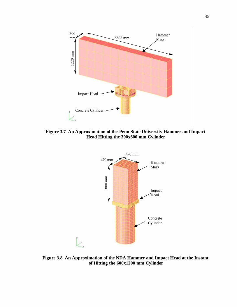
45
300mm
HammerMass
Impact Head
Concrete Cylinder
3353 mm
1220
mm
Figure 3.7 An Approximation of the Penn State University Hammer and Impact Head Hitting the 300x600 mm Cylinder
HammerMass
ImpactHead
ConcreteCylinder
470 mm470 mm
1800
mm
Figure 3.8 An Approximation of the NDA Hammer and Impact Head at the Instant of Hitting the 600x1200 mm Cylinder

46
4- The NDA tests (and their post-test models) used a thick rectangular steel plate to
distribute the impact forces from the drop hammer to the concrete cylinder, as shown
in Figure 3.7. The plate sizes were matched with the different concrete cylinder sizes.
A 25-mm rubber pad was placed between the plate and the cylinder, and another 25-
mm rubber pad was placed on top of the plate. The hammer would hit the plate,
which in turn would compress the cylinder, transferring the hammer impact load.
The Penn State University test setup (which was used in the pre-test simulations) has
a different impacting plate assembly, as shown in Figure 3.8. It is composed of a
stiffened 50-mm-thick rear plate and a 25-mm-thick front plate. A 6-mm rubber pad
was assumed to be placed between the rear and front plates. This plate assembly was
attached to the hammer’s load cell.
5- The NDA tests used a different plate with different dimensions for each specimen
size. The four sizes of plates used were 75x75x25 mm, 150x150x25 mm,
300x300x75 mm, and 600x600x75 mm for testing the 75x150 mm, 150x300 mm,
300x600 mm, and 600x1200 mm cylinder sizes, respectively.
6- The thickness of the rubber pad used between the hammer and the plate in the post-
test simulations was increased from 6 mm to 25 mm to match the actual experiment.

47
Figure 3.9 Impact Plates and Rubber Pads Used at the NDA
25-mm-thickStiffeners
Rear plateΦ 660 x 50 mm
Bottom plateΦ 660 x 25 mm
6-mm rubber
150
mm
Figure 3.10 Impact Plate Used at Penn State University
600x600x75-mm steel 300x300x25-mm steel
75x75x25-mm steel 150x150x25-
mm steel
600x600x25-mm rubber
pads
300x300x25-mm rubber
pads
150x150x25-mm rubber
pads

48
These sources of difference between the pre-test simulation results and the test results
have been corrected in the post-test simulations. The results obtained using the new
(corrected) models were used for comparison with the test results.
How the constitutive models were improved
The input parameters were modified based on the results of the static tests. For the post-
test simulations, the actual compressive strength and modulus of elasticity for a certain
cylinder size was used to model the dynamic tests for that size. The new inpur
parameters for the constitutive models are as shown in Tables (3.3) and (3.4).
Table 3.3 Input Parameters used for the Post-Test Drucker-Prager Plasticity Model
Concrete Compressive Strength, f’c Static test result for the simulated cylinder size
Mass Density, ρ 2.6x10⁻³ lb.sec2/in4
Poisson’s Ratio, ν 0.2
Young’s Elastic Modulus, E Static test result for the simulated cylinder size
Material Cohesion, dc 10% of compressive strength
Material Angle of Friction, β 51
Cap Eccentricity Parameter, R 0.65
Initial Cap Yield Surface Position 1.1x10⁻³
Transition Surface Radius Parameter, α 0.6
Ratio of Flow Stress, K 1.0
Strain Rate Effect 1.5

49
Table 3.4 Input Parameters used for the Post-Test Brittle Fracture Model
Concrete Compressive Strength, f’c Static test result for the simulated cylinder size
Mass Density, ρ 2.6x10⁻³ lb.sec2/in4
Poisson’s Ratio, ν 0.2
Young’s Elastic Modulus, E Static test result for the simulated cylinder size
Direct Stress After Cracking, σc 10% of compressive strength
Direct Cracking Strain, ec 1x10⁻³
Strain Rate Effect 1.5
3.4 Statement of Work
The work that was done by the thesis author is:
a. High-Strength Concrete:
1. Pre-test simulations
2. Post-test simulations
3. Analyses of results from the simulations and the tests.
b. Normal-Strength Concrete:
1. Pre-test simulations
2. Tests performed at Penn State University.
3. Post-test simulations
4. Analyses of results from the simulations and the tests.
Although the author did not participate in the tests that were performed at NDA, Japan
(for both high-strength and normal strength concrete), and at UBC Canada (Normal
strength concrete), the PI for the project participated in those tests.

50
The author has performed the final analyses of the results for, the high-strength and the
normal-strength concrete, as well as the comparison between the results for the two.

51
CHAPTER FOUR
INSTRUMENTATIONS AND TEST SETUP
4.1 Introduction
Test on normal and high-strength concrete cylinders were conducted at three different
locations in three different countries: Penn State University in the United States of
America, the National Defense Academy in Japan, and the University of British
Colombia in Canada. The main components of the tests in each facility were similar: a
drop hammer, a high-speed data acquisition system, sensors, and high speed
photography. These components, however, differed from place to another. Drop
hammers vary in shape, weight, and dimensions. Data acquisition systems vary in model,
make, and number of channels. Strain gages, however, remained the same since, the
same strain gages were used for all the tests conducted in all three places. Similar types
of load cells (strain based) were also used in all three places. The test setup was very
similar in the three places. The instrumented specimen was placed under the hammer and
then the hammer was allowed to fall freely and hit the specimen at velocities of, either 5
m/s, or 7 m/s. Load cells were used to measure the impact loads, accelerometers were
used to measure the hammer acceleration, and the strain gages were used to measure the
strain in the concrete.
In this section, the instrumentation suites used at each of the three testing locations are
described, with photos and illustrations provided when appropriate.

52
4.2 Drop Hammers
Drop hammers were used to apply measured impact loading to test specimens. Four drop
hammers were used in this study: the drop hammer at Penn State University (PSU), USA,
the drop hammer at the National Defense Academy (NDA) in Japan, and the two drop
hammers at the University of British Colombia (UBC) in Canada.
4.2.1 Drop hammer at Penn State University
The Max-Impact hammer (model M-4500-18) (Figure 4.1) was used to apply impact
loads to test specimens at Penn State University. The weight of the hammer (including
the impact plate and the load cells) was 6445 lbs (2930 kg). The hammer can be dropped
from a maximum 7 m (approximate). Since all sets of load cells used were the same, the
weight of the hammer remained the same during all the tests.
Hammer Components:
Figure 4.1, A show the main components of the drop hammer used at Penn State
University. A steel frame tower supported the hammer components. Mounted between
the frame and the floor were two circular stainless steel guide rails (Figure 4.1, C) on
which the hammer (Figure 4.1, A) and crosshead (Figure 4.1, B) moved. The hammer
was connected to the crosshead by a magnetic latch (Figure 4.1, D) and four mechanical
latches (Figure 4.1, E). An electric hoist (Figure 4.1, F) was used to move the crosshead.
The strike plate (Figure 4.1, G) was used to transfer the energy of the falling hammer to
the specimen and was the only portion of the hammer that contacted the specimen during
testing.

53
The hammer was secured in place by connecting safety cables (Figure 4.2, C). Each
cable was attached to the hammer using a clevis with a screw-type pin. The safety cables
were disconnected just prior to dropping the hammer during a test, and were reattached
immediately after completion of the test. The safety cables were kept connected before
any personnel entrance to the test area for any reason. The test area is defined as the area
inside the supporting frame and adjacent to the specimen.
Figure 4.1 Drop Hammer at Penn State University (back View)
A – Hammer B – Cross – Head C – Guide – Rails D – Magnetic Latch
E – Mechanical Latch F – Electrical Hoist G – Strike Plate

54
Pneumatic actuators (Figures 4.2, D and 4.3, C) were used to decelerate the hammer after
impact with the specimen. This prevented damage to the hammer and the floor beneath
the hammer. The actuators also prevented the hammer from hitting the specimen for a
second time (after possible rebound). The photoelectric sensor (Figure 4.3, A) was used
to trigger the actuators to rapidly move upward to meet the hammer. The pressurized
pneumatic cylinders acted as air springs to slow and stop the hammer.
Figure 4.2 PSU Hammer (side view)
A – Hammer B – Cross Head C – Safety Cables D – Pneumatic Actuators

55
Once the hammer was stopped, the actuators would move upward and lift the hammer
away from the specimen.
Figure 4.4 illustrates two components that were important to safe operation of the
hammer. First was the safety light (Figure 4.4, C). This light used to flash when the
control panel and sensors were properly connected and pneumatic pressure was in the
operational range. The “Panel Ready” indicator on the control panel was linked to the
safety light and would be lit under the same conditions.
Figure 4.3 Pneumatic Actuators and Photoelectric Sensor
A – Photo sensor B – Guide Rail C – Pneumatic Actuators

56
The safety light also served a second safety function by warning personnel in the area
that the system was in an operational condition so that they would stay clear of the
associated danger areas. Second, the debris curtain (Figure 4.4, D) surrounded the test
area. The purpose of the curtain was to reduce the danger associated with flying debris
when impact loading was applied to the specimen. The debris curtain surrounded the
entire test area. Two panels in the curtain included Plexiglas panels to allow video
recording of the test sequence.
Figure 4.4 Penn State Hammer (front view)
A – Hammer B – Cross – Head C – Safety Light D – Debris Curtain E – Guide Rails

57
The strike plate (Figure 4.5, A) was used to transfer the energy of the falling hammer to
the specimen either through direct steel to concrete contact or through a rubber pad that
was used, on the concrete impact interface during the soft impacts, to increase the impact
duration while reducing the peak impact load. Two load cells (Figure 4.5, B), along with
the supporting data acquisition system, were used to measure and record the impact
event. The load cells were connected to the data acquisition system using two shielded
cables. Care was taken to prevent damage to the cables from the hammer or the
specimen.
Figure 4.5 Strike Plate and Load Cells
A – Strike Plate B – Load Cells

58
4.2.2 Drop hammer at NDA, Japan
The drop hammer at the National Defense Academy in Japan (Figure 4.6) is a free fall
drop hammer that has weight of 3,041 kgs. It can drop from heights up to 30 meters.
Figure 4.7 shows a detailed diagram of different components of the NDA drop hammer
and the position of the four load cells used.
Figure 4.6 NDA Drop Hammer, Japan

59
Figure 4.7 NDA Drop Hammer’s Dimensions For each size of concrete specimen, a different size of impact plate was used to distribute
the impact forces from the hammer to the concrete. The impact plate was placed on top
of the specimen. The hammer would hit the plate, which in turn would compress the
cylinder, transferring the hammer impact load. Figure 4.8 shows the details of the impact
plates used.

60
Figure 4.8 Impact Plates Used at NDA

61
4.2.3 Drop Hammers at UBC, Canada
Two types of drop hammers were used at the University of British Colombia (UBC). The
main tests were done with the heavier of the two hammers, shown in Figure 4.9, which is
capable of dropping a 570 kg weight from heights up to 2.5 m. Figure 4.10 shows the
configuration and dimensions of the 570 kg drop hammer.
Figure 4.9 Heavy Hammer at UBC
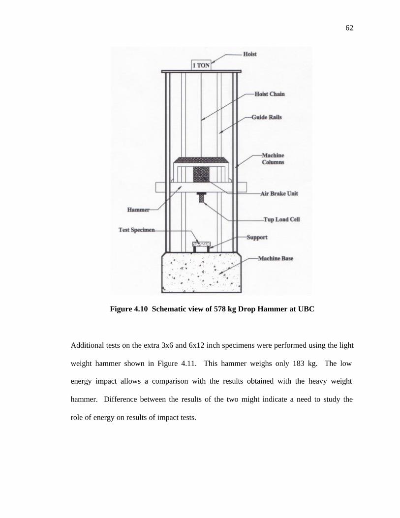
62
Figure 4.10 Schematic view of 578 kg Drop Hammer at UBC
Additional tests on the extra 3x6 and 6x12 inch specimens were performed using the light
weight hammer shown in Figure 4.11. This hammer weighs only 183 kg. The low
energy impact allows a comparison with the results obtained with the heavy weight
hammer. Difference between the results of the two might indicate a need to study the
role of energy on results of impact tests.

63
Figure 4.11 Light Weight Hammer at UBC
4.3 Response Measurement
4.3.1 Background
When selecting sensors and instrumentation for dynamic testing, a number of factors
must be considered. One factor is of particular interest in measuring dynamic responses:
speed. A data acquisition system functions as a chain and many systems parameters are

64
dependent on the weakest link in the chain. Sensors (load cells, strain gages,
accelerometers, and deflection gages) must have a mechanical and electronic response
frequency high enough to accurately transform physical phenomena into analog
electronic signals. The mechanical response of a sensor depends on the sensing element,
the structure of the sensor, and the method used to mount the sensor to the specimen.
The supporting signal conditioning must have a response frequency sufficient to
accurately amplify and transfer the sensor signals to the digitizing system. Finally, the
digitizing system must have a sampling frequency at least as high as the frequency of the
slower of the sensors and signal conditioning. In order to prevent a phenomenon known
as aliasing (mapping of a higher frequency signal to a lower frequency when acquired)
the digitizing system should have a sampling frequency at least 3 to 5 times that of the
slower of the sensors and signal conditioning. If any of these components has an
insufficient response frequency, the acquired data will be in effect damped, and critical
details of the mechanical behavior will be lost. Consequently, as a rule, filtering should
not be included in such a system without careful consideration of the impact on the
acquired data. The inability, for the most part, to implement filtering magnifies the
importance of controlling mechanical and electronic noise. In addition to the frequency
response, several other factors must be considered. The full scale range of all sensors
must be sufficient to include the maximum and minimum expected mechanical behaviors.
However, measurement resolution is a combination of full scale range of the sensor,
resolution of the digitizing equipment, and noise. The resolution of digitizing equipment
is normally expressed in bits and indicates the number of increments (2n bits) that the full
scale is divided. Excessive full scale range of a sensor can negatively impact the

65
resolution of a measurement system and affect the overall signal-to-noise ratio of a
measurement to the point that the measurements are largely meaningless. Linearity is
another factor impacting sensor and signal conditioning performance unless non-linear
calibration techniques are used. Time delays and phase shift are also important due to the
very brief nature of the events being measured (typically 1-5 ms). Time base errors that
are negligible in other structural testing (static, quasi-static, seismic, etc.) cannot be
ignored in impact testing. As a result of the sensitivity of measurements to these factors,
selecting the measurement system components and using them effectively in an impact
testing program is not a trivial task.
4.3.2 Sensors and Transducers
Several types of sensors and transducer were used with the data acquisition system:
strain-gage based load cells, strain gages for direct measurement, piezo-resistive
accelerometers, and piezoelectric accelerometers. Since all but the piezoelectric
accelerometers were strain-gage based, the function of strain gages will be addressed
first.
4.3.3 Sensor selection
Several parameters of the structural response under impact loading were measured:
applied load, acceleration of the impactor, strain in the specimen, and pneumatic actuator
activation. The following sensors were selected to measure these parameters:

66
Parameter Sensor
Applied load Strain-gage based load cells
Acceleration Piezoelectric and piezoresistive accelerometers
Concrete strain strain gages
In this section, sensors used at each of the three testing locations are described. Photos
and detailed illustrations are provided when appropriate.
4.3.3.1 Load Cells Strain gage based load cells rigidly connected to the drop hammer were used to measure
the impact loads on all three testing locations. As shown in Figure 4.12; a load cell is
made of two parts: 1) an outer (contact) part and 2) an inner part. The strike plate
transfers the load to the outer part of the load cell, which in turn transfers it to the inner
part. There is no instrumentation on the outer part. The inner part, however, is
instrumented with four strain gages mounted on its outer surface. The cross sectional
area at the center of the inner part was reduced by making it hollow; this amplifies the
signals from the reduced cross sectional area. At the unload condition, the circuit is
balanced and the output is zero. During an impact event, the inner part deforms; the
strain gage circuit becomes unbalanced and emits an output voltage.
Two different sets, consisting of two load cells each, were used during the tests
conducted at Penn State University. The first set which was used for testing the 6x12
inch (150x300 mm) and the 12x24 inch (300x600 mm) cylinders consisted of two load
cells model R-4500-700k with a capacity of 700 kip. The second set, which was used to

67
test the 24x48 inch (600x1200 mm) cylinders, consisted of a pair of National Scale
Model 1100538 load cells with a capacity of 2000 kip each. Four load cells were used at
NDA. Each load cell has a capacity of 250 kips. Only one load cell was used with each
of the two hammers at UBC. These load cells served also as the impact heads for the
hammers. Each load cell had a capacity of 220 lb (10 kN).
Figure 4.12 load cell Detail (not to scale)
4.3.3.2 Accelerometers
Two set of five accelerometers were used during the tests at Penn state University. The
first set, which consists of five Kistler piezoelectric accelerometers, with a capacity of up

68
to 5000 g, was used while testing the 6x12 (150x300 mm) cylinders. The second set
which consists of three Endevco piezoresistive accelerometers and two Kistler
piezoelectric accelerometers and has a capacity of up to 20,000 g. It was used for
measuring the hammer acceleration during the tests of the 12x24 inch (300x600 mm) and
the 24x48 inch (600x1200 mm) cylinders. The accelerometers were placed on top of the
impact plate using the accelerometer mounting buttons shown in Figure 4.13. The central
accelerometer (a piezoelectric) was used for triggering the data acquisition system and
the high speed camera.
Figure 4.13 Accelerometers Positions on top of the impact plate
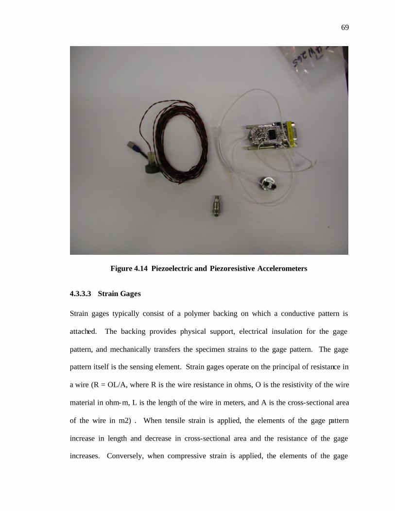
69
Figure 4.14 Piezoelectric and Piezoresistive Accelerometers
4.3.3.3 Strain Gages
Strain gages typically consist of a polymer backing on which a conductive pattern is
attached. The backing provides physical support, electrical insulation for the gage
pattern, and mechanically transfers the specimen strains to the gage pattern. The gage
pattern itself is the sensing element. Strain gages operate on the principal of resistance in
a wire (R = OL/A, where R is the wire resistance in ohms, O is the resistivity of the wire
material in ohm-m, L is the length of the wire in meters, and A is the cross-sectional area
of the wire in m2) . When tensile strain is applied, the elements of the gage pattern
increase in length and decrease in cross-sectional area and the resistance of the gage
increases. Conversely, when compressive strain is applied, the elements of the gage

70
pattern decrease in length and increase in cross-sectional area and the resistance of the
gage decreases. The relative magnitude of this change is indicated by the gage factor (a
dimensionless parameter linked to gage sensitivity).
These changes in resistance are very small in magnitude and cannot be directly measured
without difficulty. A special voltage divider circuit known as a Wheatstone bridge
(Figure 4.15) was used to transform the resistance changes into changes in voltage. The
Wheatstone bridge is comprised of two voltage divider circuits or arms that link the input
nodes (Vin+ and Vin-). A constant DC voltage (excitation voltage) is applied across the
input nodes and the bridge output voltage is measured differentially across the output
nodes (Vout+ and Vout-) and is proportional to the strain mechanically transmitted to the
active gages in the bridge. Though the bridge output voltage can be measured directly, it
was rather further conditioned through amplification and filtering due to the small
magnitude of the bridge output voltage.
Kyowa concrete strain gages type KC-80-120-A1-11L3M3R with a gage length of 84
Vin+
V in-
Vout- Vout+
Fixed Resistor Active Strain Gage
Vin+
Vin-
Vout- Vout+
V in+
Vin-
Vout- Vout+
V in+
Vin-
Vout- Vout+
¼ Bridge ½ Bridge(additive)
½ Bridge(subtractive)
Full Bridge
Vin+
V in-
Vout- Vout+
Vin+
V in-
Vout- Vout+
Vin+
V in-
Vout- Vout+
Fixed Resistor Active Strain Gage
Vin+
Vin-
Vout- Vout+
V in+
Vin-
Vout- Vout+
V in+
Vin-
Vout- Vout+
¼ Bridge ½ Bridge(additive)
½ Bridge(subtractive)
Full Bridge
Fixed Resistor Active Strain Gage
Vin+
Vin-
Vout- Vout+
Vin+
Vin-
Vout- Vout+
Vin+
Vin-
Vout- Vout+
V in+
Vin-
Vout- Vout+
V in+
Vin-
Vout- Vout+
V in+
Vin-
Vout- Vout+
V in+
Vin-
Vout- Vout+
V in+
Vin-
Vout- Vout+
V in+
Vin-
Vout- Vout+
¼ Bridge ½ Bridge(additive)
½ Bridge(subtractive)
Full Bridge
Figure 4.15 Wheatstone Bridge (Strain Gage Application)

71
mm and a gage resistance of 120 ± 1.0 ohms were used to instrument all the normal and
high-strength concrete cylinders in all tests performed in three test locations. The gage
factor for the strain gages was 2.11 ± 1.0 %.
Figure 4.16 Instrumented 300x600 Cylinder Ready for Test (PSU)
4.4 High-Speed Data Acquisition Systems
As discussed in the in sensor background, there are a number of factors to consider in
developing an overall data acquisition system for impact testing. The primary factor in
the system design is speed. Standard PC card-based data acquisition systems are
adequate for other forms of structural testing (static, quasi-static, cyclic, seismic, etc.) but

72
lack the sampling frequency necessary for impact testing. Typically, a single analog to
digital converter (ADC) is multiplexed to a number of channels. While the ADC
sampling frequency is adequate for a single channel, multiplexing the ADC to several
channels effectively shares the sampling frequency across those channels. In addition,
the switching process necessary to sequentially connect each channel requires a finite
period of time. In many systems this switching time offsets measurements on successive
channels in time, resulting in asynchronous data collection. These conditions are
unacceptable for high speed data acquisition. Similarly, the signal conditioning devices
developed for these systems are likewise inadequate for impact testing as they typically
have a response frequency on the order of 4-10 kHz. As a result, more specialized,
higher-performance hardware is required. Another factor in data acquisition system
selection is flexibility. The system developed at the Protective Technology Center (PTC)
at Penn State University consists of separate modular systems for signal conditioning and
digitizing. The modular and separate nature of these systems provides maximum
flexibility by allowing the user to select from a range of signal conditioning and
digitizing modules to meet widely varied measurement requirements.
4.4.1 Data Acquisition System at Penn State University (PSU)
A system for collecting data during impact testing has been developed for use in the
Structures Laboratory (Figure 4.17). The system consists of sensors and transducers,
custom bridge completion circuitry, a signal conditioning unit, and an A/D conversion
unit. The sampling rate used during the tests was 1 MHz for all channels.

73
Figure 4.17 Data Acquisition System at PSU
Signal Conditioning:
Signal conditioning provides power to the sensors, receives the sensor output, amplifies
that signal and passes it to the digitizer for measurement. The selected signal
conditioning system, Oasis, was manufactured by Endevco. The Oasis system consisted
of a Model 4990 amplifier rack that houses and connects the signal conditioning cards

74
and provides connection to break-out connector panels. The Model 4990 rack was
populated with two types of signal conditioning cards: Model 436 and Model 482A. The
Model 436 signal conditioning card provides excitation and amplification for strain
bridges. Bridge completion was provided externally using a custom build circuit with a
protective enclosure (Figure 4.18).
Figure 4.18 Bridge Completion Box (PSU)
Specifications for the 436 card include: The Model 482A signal conditioning card
provides constant current excitation or charge amplification and output signal
amplification for piezoelectric devices. Specifications for the 482A include: The signal
conditioning systems was configured and controlled by a PC using an Ethernet interface
and Oasis software. The Oasis software provides control of sensor sensitivity, full scale

75
input range, full scale output range, and gain. The output signals are transferred to the
digitizer through cabling connected to the output break-out panels of the Oasis system.
Figure 4.19 Endevco Oasis 2000 Signal Conditioner (PSU)
Digitizing:
The final link in the data acquisition chain is digitizing. A Win600 system manufactured
by Hi-Techniques was selected. The system consisted of a Win600 8-slot main frame
with front panel connectors and HD6114-8D digitizers boards. The main frame houses,
links, and powers the digitizing boards and provides an interface to the PC via a
proprietary interface card. The HD6114-8D digitizer boards provide 8 channels for
analog voltage inputs. Specifications include: The Win600 system was controlled using
Win600 software provided by Hi-Techniques. The software allows the user to control

76
operating parameters, perform data acquisition, transfer data to the PC, store the data to
disk, and perform post-acquisition data processing and analysis.
Figure 4.20 High-Technique Win 600 A/D Converter (PSU)
4.4.2 Data Acquisition System at the National Defense Academy (NDA)
The data acquisition system used at NDA is a Nicolet MultiPro multi channel system
(Figure 4.21) which allows acquiring multiple channel data with high speed and high
resolution. 16 channels were used during the tests, and the sampling time used was 1
micro-sec (1MHz).

77
Figure 4.21 Nicolet MultiPro Data Acquisition System
4.4.3 Data acquisition system at the University of British Colombia (UBC)
The data acquisition system consisted of a 16 channel analog to digital (A/D) converter
with a maximum sampling rate of 1 MHz if one channel is used. For multiple channel
use, the sampling rate decreases to 1/N MHz, where N is the number of active channels.
This system was built at the University of British Colombia.
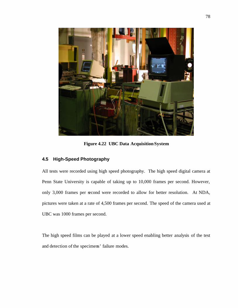
78
Figure 4.22 UBC Data Acquisition System
4.5 High-Speed Photography
All tests were recorded using high speed photography. The high speed digital camera at
Penn State University is capable of taking up to 10,000 frames per second. However,
only 3,000 frames per second were recorded to allow for better resolution. At NDA,
pictures were taken at a rate of 4,500 frames per second. The speed of the camera used at
UBC was 1000 frames per second.
The high speed films can be played at a lower speed enabling better analysis of the test
and detection of the specimens’ failure modes.

79
Figure 4.23 High-Speed Camera Used at PSU
Figure 4.24 High-speed Camera Used at NDA

80
CHAPTER FIVE
RESULTS AND DISCUSSION – HIGH-STRENGTH CONCRETE
Four different sizes of high-strength concrete (HSC) cylinders were studied under both
dynamic and static loading. The studies included both testing and parallel finite element
analysis. The finite element study included pre-test finite element simulations and
modified model post-test simulations, as described in Chapter Three.
The results of the tests, as well as the pre-test and post-test simulation predictions, are
presented and discussed next.
5.1 Pre-test Simulations
Pre-test finite element simulations using, ABAQUS EXPLICIT (version 5.8), were
carried out prior to testing in order to aid in test setup, planning and other preparations for
extracting data for the parameters that would be measured in the tests. The pre-test
simulations helped in assessing the anticipated behavior and in calibrating the equipment
and instrumentation for the tests.
As described in Chapter Three, the pre-test simulation models were developed to
represent the various specimen geometries and a general test setup based on the test
conditions at Penn State University. The material models used for concrete were a) The
Drucker-Prager Cap Plasticity model and b), The Brittle Fracture model. Each model
was used once with strain rate effects included, and once without including the strain rate
effects.

81
Each of the four cylinder sizes (75 mm x 150 mm, 150 mm x 300 mm, 300 mm x 600
mm, and 600 mm x 1200 mm, as described in Chapter Three and shown in Figure 3.1.)
was modeled eight times, as follows: Using the two concrete models, with and without
strain rate effects, and for two different drop speeds, (10 m/s and 5 m/s). The curves of
stress vs. time, and strain vs. time were extracted for each one of the 15 control elements
(described in Chapter Three and shown in Figure 3.3). This was done for each one of the
32 different simulations.
The drop hammer shape used in the pre-test simulations replicated the Pennsylvania State
University drop hammer, as shown in Figure 3.5. The main results of all these pre-test
simulations are summarized in Tables 5.1 and 5.2.
It can be seen from Tables 5.1 and 5.2 that the simulation results using strain rate effects
were almost identical to the results predicted without using strain rate effects. Hence,
only the results with strain rate effects are discussed herein.

82
Table 5.1 Pre-test Simulations Results - Rate Dependent
Cases Peak Stresses (N/mm2) Failure Strain Strain Rate
Effect Material Model
Impact Velocity (m/s)
Cylinder Size (mm)
Maximum value
Time (ms)
Minimum value
Time (ms)
Averagea value
Time (ms)
Strain**** Time (ms)
75x150 -43.27 5.08 -22.90 5.19 -22.59 5.19 -0.005 4.62 150x300 -70.28 4.88 -18.27 5.33 -24.37 4.87 -0.005 4.94 300x600 -55.97 6.81 -22.79 3.70 -28.49 6.85 -0.005 3.44
5
600x1200 -21.19 4.28 -16.38 4.83 -18.20 4.35 -0.005 4.79** 75x150 -30.43 3.41 -25.23 2.98 -21.83 2.14 -0.005 2.15
150x300 -65.13 2.51 -25.38 2.67 -36.68 2.66 -0.005 2.66 300x600 -37.03 4.64 -22.63 1.56 -22.56 4.90 -0.005 1.57
Drucker Prager Cap Plasticity
10
600x1200 -24.49 1.88 -24.17 2.68 -23.32 2.81 -0.005 1.97 75x150 -24.52 4.48 -18.65 3.82 -22.37 3.86 -0.005 5.03
150x300 -937.04 7.48 -552.58 7.49 -419.60 7.50 -0.005 6.62 300x600 -182.59 6.99 -54.74 4.58 -80.61 7.00 -0.005 7.36**
5
600x1200 -22.79 4.69 -16.36 5.83 -19.71 5.63 -0.005 3.93** 75x150 -2204.80 3.05 -1639.82 3.03 -737.23 3.05 -0.005 2.89
150x300 -3004.04 4.01 -1061.06 4.08 -2011.88 4.01 -0.005 3.24 300x600 -1364.22 4.25 -819.91 4.14 -819.91 4.25 -0.005 3.15
Rate Dependent
Brittle Fracture
10
600x1200 -72.35 4.07 -54.95 3.89 -61.38 4.08 -0.005 -*** ** Only the top part of the cylinder failed. *** No failure observed in the 15 ms time range. **** Selected based on ACI 363R-92. a Average curve generated from the three stress vs. time curves (i.e., center, edge, mid-way). Conversion factor: 1 MPa (N/mm2) = 145 psi.

83
Table 5.2 Pre-test Simulations Results – Rate Independent
Cases Peak Stresses (N/mm2) Failure Strain
Strain Rate Effect
Material Model
Impact Velocity (m/s)
Cylinder Size (mm)
Maximum value
Time (ms)
Minimum value
Time (ms)
Averagea value
Time (ms)
Strain**** Time (ms)
75x150 -43.27 5.08 -21.81 5.32 -25.79 5.15 -0.0035 4.39 150x300 -70.97 4.87 -17.70 5.33 -26.20 5.31 -0.0035 5.01 300x600 -55.97 6.81 -22.68 3.75 -29.17 6.84 -0.0035 3.33
5
600x1200 -21.08 4.32 -16.29 4.87 -18.20 4.35 -0.0035 4.57** 75x150 -30.43 3.41 -25.20 2.98 -21.62 3.02 -0.0035 2.05
150x300 -65.68 2.52 -25.38 2.67 -36.06 2.66 -0.0035 2.70 300x600 -37.37 4.64 -22.63 1.60 -22.61 4.90 -0.0035 1.55
Drucker Prager Cap Plasticity
10
600x1200 -23.11 1.92 -23.76 2.84 -23.30 2.82 -0.0035 1.88 75x150 -24.38 4.48 -18.37 3.86 -19.16 3.89 0.0035 4.67***
150x300 -937.04 7.21 -396.86 7.23 -352.77 7.22 -0.0035 6.22 300x600 -413.40 8.22 -233.57 8.17 -199.81 8.09 -0.0035 8.19
5
600x1200 -22.80 4.62 -16.41 5.76 -19.71 5.60 -0.0035 2.84 75x150 -1391.78 2.90 -771.68 2.93 -875.03 2.90 -0.0035 2.65
150x300 -2204.80 2.46 -930.15 2.46 -771.68 2.46 -0.0035 2.70 300x600 -1880.97 3.10 -840.58 3.43 -757.90 3.09 -0.0035 3.12
Rate Independent
Brittle Fracture
10
600x1200 -70.28 4.08 -54.82 4.50 -62.56 4.53 -0.0035 14.80** ** Only the top part of the cylinder failed. *** No failure observed in the 15 ms time range. **** Selected based on ACI 363R-92. a Average curve generated from the three stress vs. time curves (i.e., center, edge, mid-way). Conversion factor: 1 MPa (N/mm2) = 145 psi.

84
5.2 Tests
Impact tests were carried out at the National Defense Academy in Japan with a large drop
hammer, with a weight of 29.8 KN. The specimens tested were high-strength concrete
(100 MPa, nominal strength) cylinders of the dimensions noted in Figure 3.1. All the
concrete specimens were made of the same concrete mix. Tests were conducted at drop
speeds of 0 m/s (static tests), 5 m/s, and 7 m/s. The 10 m/s speed used in the pre-test
simulations could not be achieved since, because of local conditions, it would require
very significant data channe l rewiring. Each test was repeated three times with the same
impact velocity to obtain a varied range of results. Figures 5.1 to 5.4 show some of the
pictures taken during the tests.
The following data were collected form the tests:
1- Data obtained from static tests.
The results of the static tests are summarized in Table 5.3. The 600x1200 mm
cylinder was not tested since it was too large for the available static test machines.
The static strength value for the 600x1200 mm cylinder was calculated using the
Size Effect Law.
2- Data obtained from dynamic tests:
e) Force as a function of time at the hammer specimen interface, measured using
load cells.
f) Acceleration as a function of time at the impactors tip, measured using
accelerometers.

85
Figure 5.1 HSC Cylinder Size 600x1200 mm Before Impact. Notice the strain gauges on the side. Three lines of similar strain gauges were used, located at 1200 to each other.
Figure 5.2 Same Cylinder Broken After Impact. The steel screws on the floor were used to center the cylinder in place.
Figure 5.3 Cylinder After Impact. Most cylinders experienced a brittle splitting failure.
Figure 5.4 Same Cylinder Shown from Above. Notice the splitting lines, which were almost at 120o to each other.

86
Table 5.3 Static Tests Results
Specimen
Diameter
(mm)
Specimen
Height
(mm)
No. of
specimens
tested
Average
Weight
(kg)
Average
Specific
Weight
γ
(ton/m3)
Average
Peak
Stress
(σmax)avg.
(N/mm2)
Average
strain at
σmax
(ε0)avg.
(µe)
Average
Elastic
Modulus
(Ec)avg.
(N/mm2)
Average
Poisson
Ratio
(ν)avg.
75 150 3 1.68 2.48 89.46 1946 47,732 0.276
150 300 3 13.07 2.47 82.86 1852 47,200 0.240
300 600 3 104.1 2.42 71.10 1743 43,500 0.245
600 1200 0 * 814.3** 2.40*** 57.53*** 1653*** 35,876*** 0.243***
*No static tests were performed on the 600x1200 mm cylinder size.
** Value calculated using the Size Effect law
*** Values extrapolated from the results of the other sizes.
Conversion factor: 1 MPa (N/mm2) = 145 psi.

87
g) Strain as a function of time, measured by up to three 80-mm strain gauges placed
every 120° on the sides of the concrete cylinders, as shown in Figure 3.4. For the
75x150 mm cylinder, due to its small size, only 3 strain gages place at mid-height
of the cylinder were used.
h) High speed photography using a high speed digital camera that recorded the tests
at a speed of 4,500 frames per second. These movie were played back at a lower
speed enabling better view of what happened during the tests and how did the
specimens fail.
The results of the dynamic tests are summarized in Table 5.4. The specimens numbering
used in this Table is as explained below,
HSC - 7.5 - 5 - 1 I II III IV
I: High-strength Concrete.
II: Diameter of specimen, in cm.
III: Loading speed, in m/s.
IV: Specimen number.

88
Table 5.4 Dynamic Test Results
Test Case Impact Time at Max Top Center Bottom Velocity
(m/s) max-stress
(ms) Stress σmax
(N/mm2)
Top strain (εT)max
(10 -6 strain)
∆t
(ms) tT
∆=
•max)(ε
ε
(1/sec)
Center strain (εC)max
(10 -6 strain)
∆t
(ms) tC
∆=
•max)(ε
ε
(1/sec)
Bottom strain (εB)max
(10 -6 strain)
∆t
(ms) tB
∆=
•max)(ε
ε
(1/sec) HSC-7.5-5-1 5 5.46 -23.55 -40 5.46 -0.007 HSC-7.5-5-2 5 2.59 -27.56 -90 2.59 -0.035 HSC-7.5-5-N1 5 7.48 -58.50 -105 7.48 -0.014 HSC-7.5-5-N2 5 15.28 -107.99 -1740 15.28 -0.114 HSC-7.5-5-N3 5 5.97 -47.01 -1340 5.97 -0.224 HSC-7.5-7-N1 7 4.55 -63.11 -590 4.55 -0.130 HSC-7.5-7-N2 7 6.59 -57.92 -110 6.59 -0.017 HSC-7.5-7-N3 7 6.79 -46.16 -85 6.79 -0.013 HSC-15-5-1 5 9.70 -263.38 -2350 9.7 -0.242 -2480 9.7 -0.256 -1650 9.7 -0.170 HSC-15-5-2 5 19.60 -326.57 -750 19.6 -0.038 -480 19.6 -0.024 -80 19.6 -0.004 HSC-15-5-4 5 6.52 -239.25 -167 6.52 -0.026 -135 6.52 -0.021 -167 6.52 -0.026 HSC-15-5-N1 5 20.54 -120.22 -2290 20.54 -0.111 -1119 20.54 -0.054 -663 20.54 -0.032 HSC-15-7-N1 7 18.13 -89.67 -1923 18.13 -0.106 -2390 18.13 -0.132 -1889 18.13 -0.104 HSC-15-7-N2 7 18.34 -121.28 -1580 18.34 -0.086 -760 18.34 -0.041 -1180 18.34 -0.064 HSC-15-7-N3 7 18.23 -117.37 -2263 18.23 -0.124 -2234 18.23 -0.123 -3582 18.23 -0.196 HSC-30-5-1 5 10.77 -37.33 -535 10.77 -0.050 -677 10.77 -0.063 -585 10.77 -0.054 HSC-30-5-2 5 9.84 -40.91 -460 9.84 -0.047 -680 9.84 -0.069 -796 9.84 -0.081 HSC-30-5-3 5 10.32 -39.64 -420 10.32 -0.041 -570 10.32 -0.055 -650 10.32 -0.063 HSC-30-7-4 7 9.47 -77.31 -670 9.47 -0.071 -1050 9.47 -0.111 -780 9.47 -0.082 HSC-30-7-N1 7 8.19 -55.32 -645 8.19 -0.079 -1222 8.19 -0.149 -1579 8.19 -0.193 HSC-30-7-N2 7 7.03 -54.87 -310 7.03 -0.044 -460 7.03 -0.065 -390 7.03 -0.055 HSC-60-5-2 5 6.42 -26.07 -33 6.42 -0.005 -380 6.42 -0.059 -11 6.42 -0.002 HSC-60-5-3 5 5.56 -24.15 -35 5.56 -0.006 -420 5.56 -0.076 -6 5.56 -0.001 HSC-60-5-N 5 5.44 -19.54 -159 5.44 -0.029 -462 5.44 -0.085 -7 5.44 -0.001 HSC-6-5-4 5 5.19 -17.80 -163 5.19 -0.031 -468 5.19 -0.090 -15 5.19 -0.003 HSC-60-7-2 7 5.92 -28.57 -193 5.92 -0.033 -476 5.92 -0.080 -10 5.92 -0.002 HSC-60-7-3 7 5.76 -41.14 -151 5.76 -0.026 -717 5.76 -0.124 -20 5.76 -0.003 HSC-60-7-4 7 5.79 -42.79 -338 5.79 -0.058 -972 5.79 -0.168 -5 5.79 -0.001 HSC-60-7-5 7 5.03 -31.96 -226 5.03 -0.045 -996 5.03 -0.198 -174 5.03 -0.035 HSC-60-7-N 7 4.40 -33.60 -195 4.4 -0.044 -571 4.4 -0.130 -35 4.4 -0.008
Sign convention: (-) compressive strain; (+) tensile strain Conversion factor: 1 MPa (N/mm2) = 145 psi.
Only three strain gauges
located at mid height
were used for the
75x150mm cylinder.
Only three strain gauges
located at mid height
were used for the
75x150mm cylinder.

89
5.3 Comparison of Test and Pre-Test Simulation Results
After completion of the tests, the results of these experiments were analyzed and studied.
A significant difference was found between the pre-test finite element simulation results
and the test results.
The results obtained using Drucker-Prager Plasticity model as well as the Brittle Fracture
model, were compared with the results obtained from the impact tests at 5 m/s and 7 m/s
speeds, the static tests results, and the theoretical Size Effect model, as shown in Figures
5.5 and 5.6. These curves were plotted in logarithmic scale for comparison with Bazant’s
Size Effect curve. To understand figures 5.5 and 5.6, we calculate the logarithm of the
diameter for each cylinder (e.g. 1.875 is the log for 75mm), and the Y-axis value gives
the corresponding logarithmic strength for each of the curves.
The static strength for the 600x1200 mm cylinder was interpolated from the strength of
the other cylinders. As discussed earlier, and as can be seen from Tables 5.1 and 5.2, it
was found that the results obtained using strain rate effects and those obtained without
using strain rate effects were almost identical. For this reason, only one set of charts was
drawn and discussed. The following observations can be made from these figures
• Generally, the pre-test simulation results differed significantly from the test results.
• The tests were done with impact speeds of 5 m/s and 7 m/s, while the pre-test
simulations used impact speeds of 5 m/s and 10 m/s.

90
1
1.2
1.4
1.6
1.8
2
2.2
1.8 2 2.2 2.4 2.6 2.8 3
Log (Diameter (mm))
Log
(Stre
ngth
(MP
a))
STATIC TEST RESULT
THEORETICAL STATIC
Pre-test FEM 5m/s Impact, Druker-PragerPlasticity Model
Pre-test FEM, 10 m/s Impact Druker-Prager Plasticity Model
5 m/s IMPACT
7 m/s IMPACT
Figure 5.5 Size Effect Curves, Pre -test Simulations with Drucker-Prager Plasticity
Model Compared to Test Results
1
1.5
2
2.5
3
3.5
4
1.8 2 2.2 2.4 2.6 2.8 3
Log (Diameter (mm))
Log
(Str
engt
h (M
Pa)
)
STATIC TEST RESULT
THEORETICAL STATIC
Pre-test FEM 5m/s Impact, Brittle FractureModelPre-test FEM 10 m/s Impact, BrittleFracture Model
5 m/s IMPACT
7 m/s IMPACT
Fig. 5.6 Size Effect Curves, Pre-test Simulations with Brittle Fracture Model
Compared to Test Results

91
These data indicated that a Size Effect existed for compressively loaded high-strength
concrete cylinders under both static and dynamic loads. Generally, as the size of the
specimen increased, the apparent strength of the concrete decreased.
• A variation of concrete strength with the variation of the loading rate was observed.
Although this phenomenon was observed and discussed in abundance, it can be
stated that the present results provide more data that can add to that data base.
• The static loading curve and the theoretical curve were close to one another and they
almost had the same shape.
• The concrete strength values recorded when the impact speed was 7 m/s were higher
than the values recorded when the impact speed was 5 m/s for all sizes of concrete
cylinders. However, the strength values obtained for the 7 m/s impact were lower
than the static test strength values for all cylinder sizes, except for the 6x12 mm
cylinder. This may be due to the conflicting actions of the Size Effect phenomenon
and the loading rate phenomenon. This observation needs to be studied further.
• The results of the 75x150 mm cylinder were considerably below the expected values
(compare with the simulation results). This may be due to the fact that the energies
associated with the impact were very high for this small cylinder size to withstand. It
seems that the cylinder may have shattered at stress values lower than the actual
strength.
• Accordingly, the closeness of the experimental results between the 5 m/s and 7 m/s
impacts for the 75x150 mm cylinder might be a result of the condition described
above.

92
• If the results for the 75x150 mm cylinder were disregarded, since it is believed not to
represent the actual values, the curves for the 7 m/s and the 5 m/s results are almost
parallel to each other, with the values of the 7 m/s stay at an almost constant distance
above those of the 5 m/s.
• The pre-test simulation results obtained using the Drucker-Prager plasticity model
for concrete differ significantly from the results obtained using the Concrete Brittle
Fracture model.
• For the Drucker-Prager model, the results obtained for the 5 m/s impact speed were
higher than those obtained for the 10 m/s impact speed. However, for the Brittle
Fracture model, the results for the 5 m/s impact were lower than those for the 10 m/s
impact. For the test results the strength values obtained for the 7 m/s impact velocity
are higher than those obtained with the 5 m/s impact velocity.
• The strength values obtained, using the Brittle Fracture model, were very high, as
compared with the test results and the results obtained using the Drucker-Prager
model.
The obvious difference between the test results and the pre-test simulations showed that
one had to perform post-test finite element simulations to correct the parameters that may
have contributed to these differences.
5.4 Post-test simulations
The comparison between the test results and the pre-test simulations results revealed the
necessity to redo the simulations trying, as much as possible, to decrease the differences

93
between the test results and the simulation results. Bearing in mind the differences
between the test setup at Penn State University and at the NDA, the finite element model
was modified to match the test setup at the NDA. Changes were made to the hammer
shape and its dimensions to match those at the NDA. The impact interface conditions
such as the shape and dimensions of the impacting plate, the thickness of the rubber pad,
changed from those at Penn State to the ones used actually during the tests at the NDA.
A different impacting plate size was used for each different cylinder size. The 10 m/s
impact velocity was replaced with the actually used 7 m/s velocity, while the 5 m/s
velocity was kept.
The concrete models parameters were modified using the results from the static tests.
Since no difference was found between the strain rate dependent model and the non rate
dependent model, only the strain rate dependent model was used for the post-test
simulations and the related analysis and discussion.
The results of the post-test simulations, performed using ABAQUS version 5.8, are
summarized in Table 5.5.
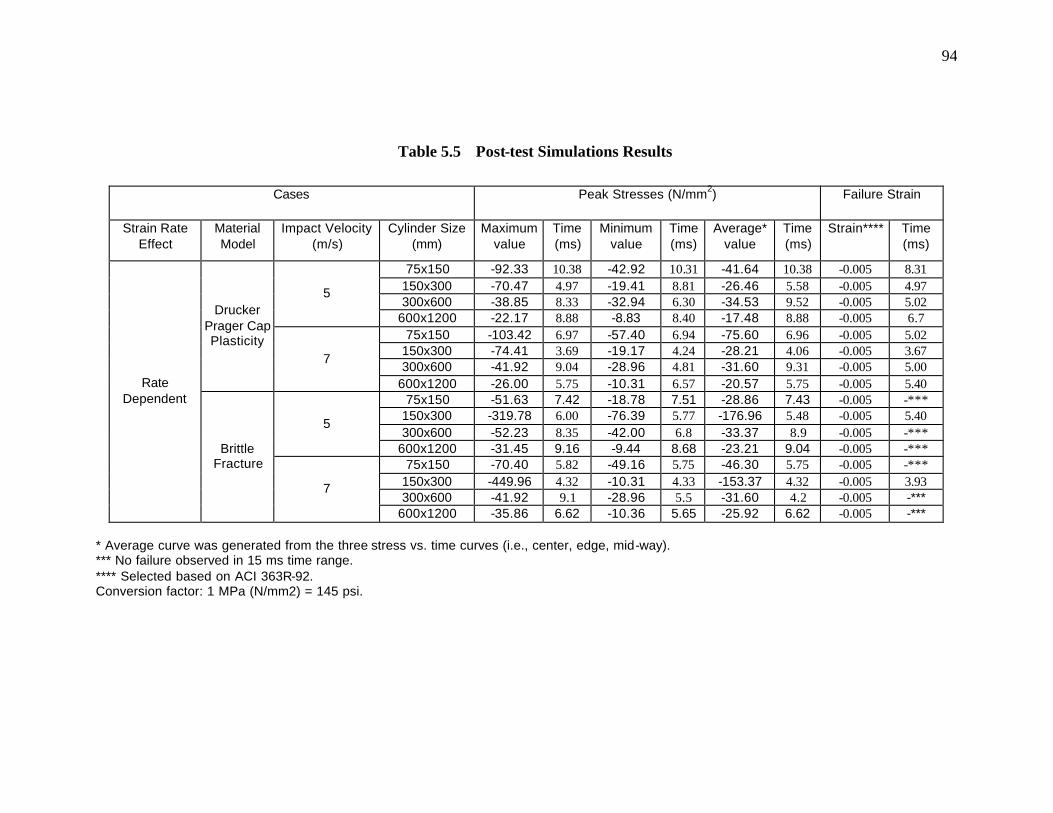
94
Table 5.5 Post-test Simulations Results
Cases Peak Stresses (N/mm2) Failure Strain
Strain Rate Effect
Material Model
Impact Velocity (m/s)
Cylinder Size (mm)
Maximum value
Time (ms)
Minimum value
Time (ms)
Average* value
Time (ms)
Strain**** Time (ms)
75x150 -92.33 10.38 -42.92 10.31 -41.64 10.38 -0.005 8.31 150x300 -70.47 4.97 -19.41 8.81 -26.46 5.58 -0.005 4.97 300x600 -38.85 8.33 -32.94 6.30 -34.53 9.52 -0.005 5.02
5
600x1200 -22.17 8.88 -8.83 8.40 -17.48 8.88 -0.005 6.7 75x150 -103.42 6.97 -57.40 6.94 -75.60 6.96 -0.005 5.02
150x300 -74.41 3.69 -19.17 4.24 -28.21 4.06 -0.005 3.67 300x600 -41.92 9.04 -28.96 4.81 -31.60 9.31 -0.005 5.00
Drucker Prager Cap Plasticity
7
600x1200 -26.00 5.75 -10.31 6.57 -20.57 5.75 -0.005 5.40 75x150 -51.63 7.42 -18.78 7.51 -28.86 7.43 -0.005 -***
150x300 -319.78 6.00 -76.39 5.77 -176.96 5.48 -0.005 5.40 300x600 -52.23 8.35 -42.00 6.8 -33.37 8.9 -0.005 -***
5
600x1200 -31.45 9.16 -9.44 8.68 -23.21 9.04 -0.005 -*** 75x150 -70.40 5.82 -49.16 5.75 -46.30 5.75 -0.005 -***
150x300 -449.96 4.32 -10.31 4.33 -153.37 4.32 -0.005 3.93 300x600 -41.92 9.1 -28.96 5.5 -31.60 4.2 -0.005 -***
Rate Dependent
Brittle Fracture
7
600x1200 -35.86 6.62 -10.36 5.65 -25.92 6.62 -0.005 -*** * Average curve was generated from the three stress vs. time curves (i.e., center, edge, mid-way). *** No failure observed in 15 ms time range. **** Selected based on ACI 363R-92. Conversion factor: 1 MPa (N/mm2) = 145 psi.
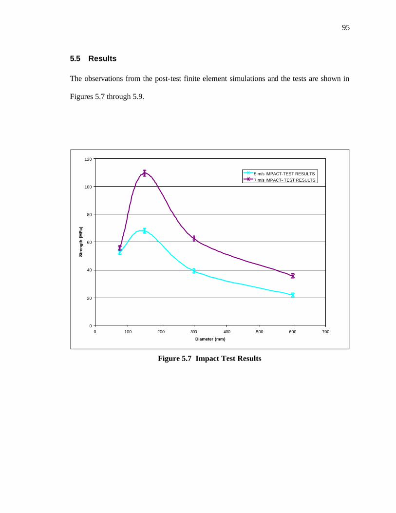
95
5.5 Results
The observations from the post-test finite element simulations and the tests are shown in
Figures 5.7 through 5.9.
0
20
40
60
80
100
120
0 100 200 300 400 500 600 700
Diameter (mm)
Str
engt
h (M
Pa)
5 m/s IMPACT-TEST RESULTS7 m/s IMPACT- TEST RESULTS
Figure 5.7 Impact Test Results
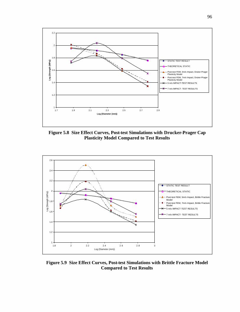
96
1
1.2
1.4
1.6
1.8
2
2.2
1.7 1.9 2.1 2.3 2.5 2.7 2.9
Log (Diameter (mm))
Lo
g (
Str
eng
th (
MP
a))
STATIC TEST RESULT
THEORETICAL STATIC
Post-test FEM, 5m/s Impact, Druker-PragerPlasticity Model
Post-test FEM, 7m/s Impact, Druker-PragerPlasticity Model
5 m/s IMPACT-TEST RESULTS
7 m/s IMPACT- TEST RESULTS
Figure 5.8 Size Effect Curves, Post-test Simulations with Drucker-Prager Cap
Plasticity Model Compared to Test Results
1
1.2
1.4
1.6
1.8
2
2.2
2.4
2.6
1.8 2 2.2 2.4 2.6 2.8 3
Log (Diameter (mm))
Log
(Stre
ngth
(MP
a))
STATIC TEST RESULT
THEORETICAL STATIC
Post-test FEM, 5m/s Impact, Brittle FractureModelPost-test FEM, 7m/s Impact, Brittle FractureModel5 m/s IMPACT-TEST RESULTS
7 m/s IMPACT- TEST RESULTS
Figure 5.9 Size Effect Curves, Post-test Simulations with Brittle Fracture Model Compared to Test Results

97
Figure 5.7 shows the experimental curves for the 5 m/s and 7 m/s speeds. These curves
are based on the total average of all test results. The vertical data range lines show the
range of distribution of the test data. The top of the vertical data range line shows the
highest strength value obtained while, the bottom of the vertical data range line shows the
lowest strength value obtained from the test results.
In Figures 5.8 and 5.9, the logarithm of strength (in MPa.) is plotted against the logarithm
of the specimen size (in mm) for the following cases:
1. Experimental results obtained for an impact velocity of 7 m/s.
2. Experimental results for an impact velocity of 5 m/s.
3. Static test results.
4. Results calculated using Bazant’s Size Effect law3.
5. Post- test results obtained using the finite element simulation for an impact velocity
of 5 m/s.
6. Post- test results obtained using the finite element simulation for an impact velocity
of 7 m/s.
5.6 Discussion of Results
The following observations can be made from the above figures:
• These data indicate that a Size Effect exists for compressively loaded high-strength
concrete cylinders under both static and dynamic loads. Generally, as the size of the
specimen increased, the apparent strength of the concrete decreased.

98
• A variation of concrete strength with the variation of the loading rate was observed.
Although this phenomenon has been observed and discussed in abundance, it can be
stated that the result s provide more data that can add to that data base.
• The static loading curve and the theoretical curve were close to one another and they
almost had the same shape.
• The concrete strength values, recorded when the impact speed was 7 m/s, were higher
than the values recorded when the impact speed was 5 m/s for all sizes of concrete
cylinders. However, the strength values obtained for the 7 m/s impact were lower
than the static test strength values for all cylinder sizes, except for the 150x300 mm
cylinder. This may be due to the conflicting actions of the Size Effect phenomenon
and the loading rate phenomenon. This observation needs to be studied further.
• The results of the 75x150 mm cylinder were considerably below the expected values
(compare with the simulation results). This may be due to the fact that the energies
associated with the impact were very high for this small cylinder size to withstand. It
seems that the cylinder may have shattered at stress values lower than the actual
strength.
• Accordingly, the nearness of the results between the 5 m/s and 7 m/s impacts for the
75x150 mm cylinder might be a result of this condition.
• If the results for the 75x150 mm cylinder were disregarded, since it is believed not to
represent the actual values, the curves for the 7 m/s and the 5 m/s results are almost
parallel to each other, with the values of the 7 m/s lay at an almost constant distance
above those of the 5 m/s.
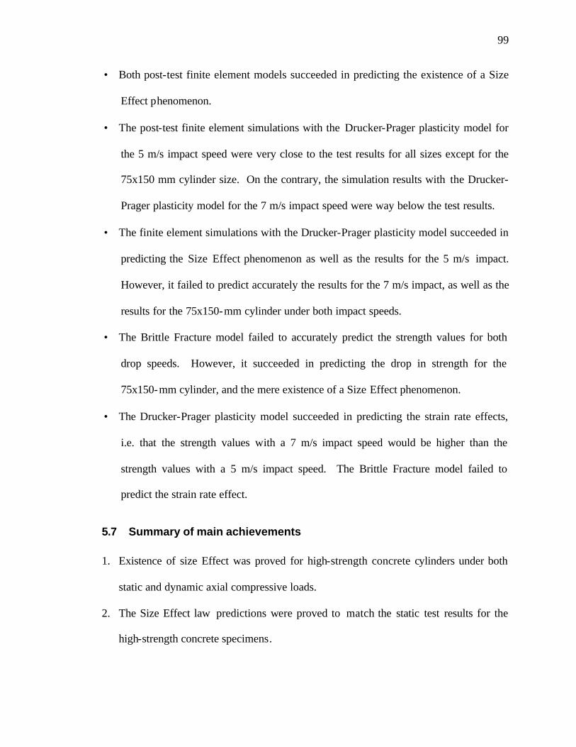
99
• Both post-test finite element models succeeded in predicting the existence of a Size
Effect phenomenon.
• The post-test finite element simulations with the Drucker-Prager plasticity model for
the 5 m/s impact speed were very close to the test results for all sizes except for the
75x150 mm cylinder size. On the contrary, the simulation results with the Drucker-
Prager plasticity model for the 7 m/s impact speed were way below the test results.
• The finite element simulations with the Drucker-Prager plasticity model succeeded in
predicting the Size Effect phenomenon as well as the results for the 5 m/s impact.
However, it failed to predict accurately the results for the 7 m/s impact, as well as the
results for the 75x150-mm cylinder under both impact speeds.
• The Brittle Fracture model failed to accurately predict the strength values for both
drop speeds. However, it succeeded in predicting the drop in strength for the
75x150-mm cylinder, and the mere existence of a Size Effect phenomenon.
• The Drucker-Prager plasticity model succeeded in predicting the strain rate effects,
i.e. that the strength values with a 7 m/s impact speed would be higher than the
strength values with a 5 m/s impact speed. The Brittle Fracture model failed to
predict the strain rate effect.
5.7 Summary of main achievements
1. Existence of size Effect was proved for high-strength concrete cylinders under both
static and dynamic axial compressive loads.
2. The Size Effect law predictions were proved to match the static test results for the
high-strength concrete specimens.
100
3. Higher loading rates were found to enhance the apparent strength of high-strength
concrete specimens.
4. Two finite element models were developed using ABAQUS EXPLICIT version 5.8.
The first is a modified Drucker-Prager Cap Plasticity model; the second is a Brittle
Fracture model. Both post-test finite element models, which were fine-tuned using
the results of the static tests for each cylinder size, succeeded in predicting the
existence of a Size Effect phenomenon. The Drucker-Prager model predictions
almost matched the impact test results; the Brittle Fracture model results were less
accurate, but agreed with the impact tests within acceptable limits.

101
CHAPTER SIX
RESULTS AND DISCUSSION – NORMAL-STRENGTH CONCRETE
Four different sizes of geometrically similar normal-strength concrete cylinders (3 inch x
6 inch, 6 inch x 12 inch, 12 inch x 24 inch, and 24 inch x 48 inch, as described in Chapter
Three and shown in Figure 3.2.) were studied under both dynamic and static loading.
The dynamic domain study can be further divided according to the impact interface
conditions used, as follows; a) Soft Impact: In which rubber pads were placed on top of
the concrete cylinders to cushion the hammer impacts; and b) Hard Impact: In which the
hammer impacted the concrete specimens directly with no rubber pad in between.
The studies included both experimental testing and parallel finite element stud ies. The
finite element stud ies included pre-test finite element simulations and modified model
post-test simulations, as explained in detail in Chapter Three.
All the results and calculations of the study on the normal-strength concrete cylinders
were performed using English units. However, to match the general format of the thesis,
and to allow for comparison with the high-strength concrete results, the results of the
tests and the simulations of the normal strength concrete cylinder will be presented in SI
units.
The results of the static tests, the dynamic tests (both hard and soft impact tests), as well
as the pre-test and post-test simulations for the normal-strength concrete cylinders are
presented and discussed in this chapter.

102
6.1 Pre-test Simulations
Results of the pre-test simulations, which were carried out before the tests in order to help
in preparations for the tests, are presented here. ABAQUS EXPLICIT (version 5.8) was
used in the pre-test simulations.
As described in Chapter Three, the pre-test simulation models were developed to
represent the various specimen geometries and a general test setup based on the test
conditions at Penn State University. The material models used for concrete were a) The
Modified Drucker-Prager Cap Plasticity model and b), The Brittle Fracture model. Each
model was used once with strain rate effects included, and once without including the
strain rate effects.
The pre-test simulations were divided into two parts: a) hard impact modeling, and b)
soft impact modeling.
For each type of impact (soft or hard), each one of the four cylinder sizes was modeled
twelve times using the two concrete models, with and without strain rate effects, and for
three different drop speeds, (10 m/s, 5 m/s, and 1 m/s). The curves of stress vs. time, and
strain vs. time were extracted for each one of the 15 control elements (described in
Chapter three and shown in Figure 3.3). This was done for each one of the 96 different
simulations.

103
6.1.1 Hard Impact Pre-Test Simulations
Results of the hard impact pre-test simulations are presented in Tables 6.1 and 6.2. Table
6.1 includes the results obtained from the pre-test simulations without including strain
rate effects, while Table 6.2 includes the results obtained with simulations that included
strain rate effects.
It can be seen from Tables 6.1 and 6.2 that the simulation results using strain rate effects
were almost the same as the results without using strain rate effects. Hence, only the
results with strain rate effects will be discussed.
6.1.2 Soft Impact Pre-Test Simulations
The soft impact results are presented in Tables 6.3 and 6.4. Table 6.3 includes the results
obtained from the pre-test simulations without including strain rate effects, while Table
6.4 includes the results obtained with simulations that take strain rate effects into account.
Similar to the hard impact simulations, including strain rate effects into the soft impact
simulations did not have a significant effect, as can be seen from Tables 6.3 and 6.4.

104
Table 6.1 Pre-test Simulations – Hard Impact Results – No Strain Rate Effects
Cases Peak Stresses (MPa) Failure Strain
Strain Rate Effect
Material Model Impact Velocity Model
Dimensions Max. Curve Time (ms) Min. Curve Time
(ms) Avg. Curve Time (ms) Strain Time
(ms)
75x150 mm 25.88 .00548 23.96 .00548 24.55 .00548 0.003 .0116
150x300 mm 27.70 .00771 26.13 .00594 26.62 .00594 0.003 .0119
300x600 mm 28.57 .00792 23.39 .00792 28.07 .00792 0.003 .0139 10 m/s
600x1200 mm 30.46 .0381 28.10 .0139 29.10 .0218 0.003 0.310
75x150 mm 19.55 .0073 17.12 .00548 17.93 .00548 0.003 .0307
150x300 mm 21.80 .00792 19.90 .00792 20.69 .00792 0.003 .0874
300x600 mm 23.05 0.0099 21.33 0.0079 22.14 .0099 0.003 .420 5 m/s
600x1200 mm 23.35 .0238 21.44 .0198 22.28 .0238 0.003 0.823
75x150 mm 6.41 .011 5.95 .011 6.22 .011 0.003 .454
150x300 mm 6.43 .0199 6.08 .0199 6.30 .0199 0.003 .887
300x600 mm 17.16 7.6 9.66 2 9.66 7.6 -* -*
Drucker-Prager
1 m/s
600x1200 mm 6.53 1.58 5.13 .0238 5.53 1.77 -* -*
75x150 mm 70.34 .0146 62.58 .0128 67.03 .0128 0.003 .0929
150x300 mm 65.50 .0119 61.68 .0119 63.93 .0119 0.003 .199
300x600 mm 67.27 .0119 59.21 .0119 63.10 .0119 0.003 .806 10 m/s
600x1200 mm 56.09 .0238 50.60 .0238 52.67 .0238 0.003 .95
75x150 mm 35.00 .0128 30.93 .0146 33.28 .0146 0.003 .128
150x300 mm 68.79 .208 38.36 .198 47.03 .205 0.003 1.12
300x600 mm 33.64 .0119 29.61 .0119 31.59 .0119 0.003 .434 5 m/s
600x1200 mm 28.06 .0238 25.67 .0238 26.41 .0238 0.003 3.01
75x150 mm 123.45 6.43 27.60 4.24 58.48 5.79 0.003 2.63
150x300 mm 123.45 5.98 27.60 4.21 58.28 4.81 0.003 2.64
300x600 mm 17.30 .723 4.96 .386 8.83 .386 -* -*
Rate Independent
Brittle Fracture
1 m/s
600x1200 mm 10.23 2.85 6.76 2.85 7.39 2.85 -* -*
* No failure observed in 15 ms time range. ** May have failed under a lower strain value.a generated from the three stress vs. time curves (i.e., center, edge, mid-way). 1 MPa=145 psi

105
Table 6.2 Pre-test Simulations – Hard Impact Results – Strain Rate Effects included
Cases Peak Stresses (MPa) Failure Strain
Strain Rate Effect
Material Model Impact Velocity Model
Dimensions Max. Curve Time (ms) Min. Curve Time
(ms) Ave. Curve Time (ms) Strain Time
(ms)
75x150 mm 25.88 .00548 23.96 .00548 24.55 .00548 .0045 .0174
150x300 mm 27.70 .00771 26.21 .00594 26.62 .00594 .0045 .0227
300x600 mm 28.57 .00792 27.52 .00792 28.07 .00792 .0045 .029 10 m/s
600x1200 mm 30.48 .0349 28.10 .0158 29.10 .0218 .0045 .422
75x150 mm 19.55 .0073 17.12 .00548 17.92 .00548 .0045 .049
150x300 mm 21.80 .00792 19.90 .00792 20.69 .00792 .0045 .134
300x600 mm 23.05 .0099 21.33 .00792 22.14 .00792 .0045 .509 5 m/s
600x1200 mm 23.35 .0238 21.44 .0198 22.28 .0238 .0045 .962
75x150 mm 6.41 .011 5.95 .011 6.22 .011 .0045 .546
150x300 mm 6.43 .0118 6.08 .0118 6.30 .0118 .0045 1.04
300x600 mm 17.17 7.6 9.87 1.99 9.63 7.6 -* -*
Drucker-Prager
1 m/s
600x1200 mm -6.53 .0158 -5.13 .0238 -5.53 .0177 -* -*
75x150 mm 70.34 .0128 61.95 .0128 66.45 .0128 .0045 .0929
150x300 mm 65.50 .0119 61.68 .0119 63.93 .0119 .0045 .741
300x600 mm 77.24 .406 27.54 .384 44.55 .39 -** -** 10 m/s
600x1200 mm 56.09 .0238 50.60 .0238 52.67 .0238 .0045 8.78
75x150 mm 34.98 .01 30.71 .011 32.90 .0128 .0045 .549
150x300 mm 68.91 .205 36.30 .198 46.97 .205 .0045 1.19
300x600 mm 33.64 .0119 30.36 .0099 31.59 .0099 -* -* 5 m/s
600x1200 mm 28.06 .0238 25.17 .0198 26.34 .0238 -* -*
75x150 mm 17.75 6.51 99.31 4.95 133.10 6.04 0.0045 3.19
150x300 mm 89.66 5.81 18.79 3.63 43.03 4.25 -* -*
300x600 mm 21.49 2.38 6.34 2.36 15.52 1.97 -* -*
Rate Dependent
Brittle Fracture
1 m/s
600x1200 mm 10.29 2.84 6.76 2.85 7.39 2.85 -* -*
* No failure observed in 15 ms time range. ** May have failed under a lower strain value.a generated from the three stress vs. time curves (i.e., center, edge, mid-way). 1 MPa=145 psi

106
Table 6.3 Pre-test Simulations – Soft Impact Results – No Strain Rate Effects
Cases Peak Stresses (MPa) Failure Strain
Strain Rate Effect
Material Model Impact Velocity Model
Dimensions Max. Curve Time (ms) Min. Curve Time
(ms) Avg. Curve Time (ms) Strain Time
(ms)
75x150 mm 7.45 1.68 7.27 1.72 7.34 1.69 0.003 1.2
150x300 mm 11.58 3.97 6.94 3.97 7.93 4.0 0.003 .971
300x600 mm 11.08 1.35 7.54 1.22 8.97 1.35 0.003 .961 10 m/s
600x1200 mm 12.37 1.75 9.50 1.48 10.90 1.61 0.003 1.27
75x150 mm 5.99 4.67 5.83 4.76 5.91 4.65 0.003 2.45
150x300 mm 19.12 5.9 5.68 6.82 7.45 6.35 0.003 2
300x600 mm 8.39 2.49 5.28 1.95 6.41 2.45 0.003 1.65 5 m/s
600x1200 mm 8.65 2.69 6.52 1.87 7.45 2.74 0.003 2.07
75x150 mm 5.35 10.3 4.75 15 4.89 15 0.003 11.1
150x300 mm 6.65 15 5.04 9.76 -4.54 12.4 -* -*
300x600 mm 5.33 10.7 3.63 6.21 4.25 10.7 0.003 7.06
Drucker-Prager
1 m/s
600x1200 mm 3.72 6.57 2.73 5.91 3.27 5.99 -* -*
75x150 mm 59.95 2.26 41.92 2.23 49.66 2.23 0.003 2.5
150x300 mm 26.39 2.2 11.62 1.24 15.17 1.84 0.003 3.03
300x600 mm 0.08 2.4 29.86 2.31 56.83 2.4 0.003 2.94 10 m/s
600x1200 mm 86.90 4.46 70.34 4.65 7.31 4.36 0.003 9.68
75x150 mm 24.21 4.46 18.48 3.86 22.32 3.88 -* -*
150x300 mm 48.28 4.53 8.10 2.32 33.86 4.99 0.003 5.46
300x600 mm 64.68 5 23.63 4.21 38.97 4.75 0.003 3.82 5 m/s
600x1200 mm 21.34 4.8 16.45 5.98 18.91 5.64 -* -*
75x150 mm 14.44 15 8.39 15 10.14 15 -* -*
150x300 mm 5.52 9.69 5.19 15 4.10 12.5 -* -*
300x600 mm 18.90 14.5 11.14 14.3 11.66 14.6 -* -*
Rate Independent
Brittle Fracture
1 m/s
600x1200 mm 3.71 6.58 2.71 5.78 3.26 6.03 -* -*
* No failure observed in 15 ms time range. ** May have failed under a lower strain value.a generated from the three stress vs. time curves (i.e., center, edge, mid-way). 1 MPa=145 psi

107
Table 6.4 Pre-test Simulations – Soft Impact Results – Strain Rate Effects Included
Cases Peak Stresses (MPa) Failure Strain
Strain Rate Effect
Material Model Impact Velocity Model
Dimensions Max. Curve Time (ms) Min. Curve Time
(ms) Avg. Curve Time (ms) Strain Time
(ms)
75x150 mm 7.45 1.68 7.26 1.71 7.34 1.69 0.0045 1.26
150x300 mm 11.62 3.94 9.60 3.71 7.93 3.99 0.0045 .971
300x600 mm 11.08 1.35 7.54 1.2 8.97 1.35 0.0045 1.03 10 m/s
600x1200 mm 12.37 1.75 9.50 1.48 10.90 1.61 0.0045 1.39
75x150 mm 5.99 4.67 5.83 4.76 5.91 4.69 0.0045 2.52
150x300 mm 19.17 5.88 6.41 9.11 7.45 6.28 0.0045 2
300x600 mm 8.39 2.49 5.29 1.76 6.41 2.46 0.0045 1.74 5 m/s
600x1200 mm 8.66 2.61 6.55 1.86 7.48 2.68 0.0045 2.23
75x150 mm 5.34 10.3 4.75 15 4.89 15 0.0045 11.3
150x300 mm 6.65 14.96 5.04 9.77 4.53 12.42 -* -*
300x600 mm 5.32 10.6 3.63 6.39 4.25 10.7 0.0045 7.6
Drucker-Prager
1 m/s
600x1200 mm 3.72 6.57 2.73 5.91 3.27 5.99 -* -*
75x150 mm 60.12 2.24 42.59 2.21 49.72 2.23 0.0045 2.66
150x300 mm 24.77 2.2 11.63 1.2 14.97 1.83 0.0045 3.14
300x600 mm 62.07 2.18 62.07 2.6 62.07 2.55 0.0045 3.02 10 m/s
600x1200 mm 75.86 4.53 59.43 4.43 73.10 4.55 -* -*
75x150 mm 24.98 4.48 18.68 3.82 0.02 3.85 0.0045 5.17
150x300 mm 10.16 3.76 8.10 2.32 7.31 2.95 0.0045 6.77
300x600 mm 64.74 4.59 24.96 4.51 37.59 4.62 0.0045 6.76 5 m/s
600x1200 mm 22.30 4.63 16.74 5.41 19.24 4.64 -* -*
75x150 mm 14.44 15 8.39 15 10.14 15 -* -*
150x300 mm 5.52 9.69 5.19 15.00 4.10 12.5 -* -*
300x600 mm 7.68 12.2 7.20 12.7 7.38 12.2 -* -*
Rate Independent
Brittle Fracture
1 m/s
600x1200 mm 3.71 6.58 2.71 5.78 3.26 6.03 -* -*
* No failure observed in 15 ms time range. ** May have failed under a lower strain value.a generated from the three stress vs. t ime curves (i.e., center, edge, mid-way). 1 MPa=145 psi

108
6.2 Tests
Impact tests on normal-strength concrete cylinders were performed at three different
places. The main tests were carried out at the structures lab of The Pennsylvania State
University in the United States, the sizes tested were the 6x12 inch (150x300 mm), 12x24
inch (300x600 mm), and 24x48 inch (600x1200 mm). Additional tests on the 12x24 inch
(300x600 mm) and the 24x48 inch (600x1200 mm) cylinders were performed at the
National Defense Academy, Japan. The 3x6 inch (75x150 mm) cylinders were tested at
the University of British Colombia, Canada, along with some additional tests on the 6x12
inch (150x300 mm) cylinders. The specimens tested were 6,943 psi (47.88 MPa) normal-
strength concrete cylinders of the dimensions noted in Figure 3.1. All the concrete
specimens were made of the same concrete mix and cast at the same time. Tests were
conducted at drop speeds of 0 m/s (static tests), 5 m/s, and 7 m/s. The 10 m/s speed used
in the pre-test simulations could not be achieved in any of the three locations, so the 7
m/s velocity was used instead. Each test was repeated three times with the same impact
velocity and the same interface condition (soft or hard impact) to obtain a varied range of
results.
All the static tests on normal strength concrete cylinders were performed at the
University of British Colombia, Canada.
The specimens were stored in a completely dry environment for two years before being
tested. This insured that the specimens were completely dry at the time of the tests, and
eliminated the effect of drying rate on the results obtained. Static tests were carried out

109
simultaneously with the impact tests to avoid having results at different time for each
type of test.
6.2.1 Static Tests Results
The results of the static tests are summarized in Table 6.5. No static test was performed
on the 12x24 inch (600x1200 mm) cylinder size since it was too large for the static test
machines available. The static strength values for the 12x24 inch (600x1200) cylinder
size were extrapolated from the strength values for the other cylinder sizes.
Table 6.5 Static Tests Results
Specimen
Diameter
(mm)
Specimen
Height
(mm)
No. of
specimens
tested
Average
Peak
Stress
(σmax)avg.
(N/mm2)
Average
strain at
σmax
(ε 0)avg.
Average
Elastic
Modulus
(Ec)avg.
(N/mm2)
75 150 3 42.58 0.0018716 27305.64
150 300 3 47.88 0.0020326 30844.30
300 600 3 44.81 0.002049 25066.39
600 1200 0 ¥ 40.1 $ 0.002065* 19288.48*
¥ No static tests were performed on the 600x1200 mm cylinder size.
$ Value calculated using the static Size Effect Law.
* Values Extrapolated from the results of the other sizes.
Conversion factor 1 MPa (N/mm2) = 145 psi

110
6.2.2 Dynamic Tests Results
The results of the dynamic tests performed at each location will be presented separate
first and then they will be combined together for each type of interface condition (soft or
hard).
6.2.2.1 Dynamic Tests Performed at Penn State University
These are the main impact tests. Three cylinder sizes were tested: 6x12 inch (150x300
mm), 12x24 inch (300x600 mm), and 24x48 inch (600x1200 mm). The proposed tests on
the 3x6 inch (75x150 mm) cylinders were conducted at UBC, Canada, for the reasons
explained in Chapter Three. Two types of tests were performed: Hard impact tests and
soft impact tests. The proposed tests on the 24x48 inch (600x1200 mm) cylinders were
not completed. The 24x48 inch (600x1200) cylinders were found to be too much for the
hammer to break with a single impact. Several tests were done using multiple hits at 5
m/s impact velocity—for both hard and soft impacts—and for the soft impact with a 7
m/s velocity. Only one hard impact with a 7 m/s impact velocity was done; it cracked the
specimen but did not break it. The massive force that was generated from the impact
forced us to abandon doing the rest of the tests on the 24x48 inch (600x1200 mm)
cylinder with the 7 m/s impact velocity.
Figure 6.1 to 6.8 show some of the pictures taken during the tests performed at Penn State
University.

111
Figure 6.1 Concrete Base Used to Mount Small Size Specimens
Figure 6.2 3x6, 6x12, and 12x24 inch Specimens Ready for Gauging – Front View
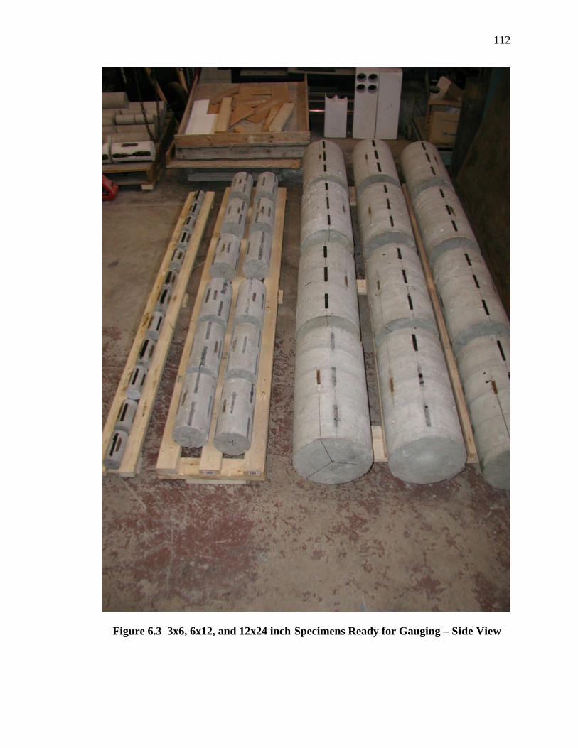
112
Figure 6.3 3x6, 6x12, and 12x24 inch Specimens Ready for Gauging – Side View

113
Figure 6.4 75x150 mm Specimen Before Test
Figure 6.5 Remaining Bottom Cone and Side of the Same Specimen after Test

114
Figure 6.6 300x600 mm Specimen Ready for Hard Impact Test
Figure 6.7 Same Specimen after Test – Notice the Remaining Top Cone

115
Figure 6.8 600x1200 mm Specimen Ready for Soft Impact Test

116
For each test, the following data was collected:
i) Force vs. time at the hammer specimen interface, measured using the load cells.
j) Acceleration vs. time of the impact tip, measured using accelerometers.
k) Strain vs. time, measured by up to nine 80-mm strain gauges placed at 120° on the
sides of the concrete cylinders, as shown in Figure 3.4. For the 75x150 mm
cylinder, due to its small size, only 3 strain gauges place at mid-height of the
cylinder were used.
l) High speed photography using a high speed digital camera that is capable of
taking up to 10,000 frames per second, and can be played back at a lower speed
enabling better view of what happened during the test and how did the specimen
fail.
The results of the dynamic tests at Penn State University are summarized in Tables 6.6 to
6.9. The specimens numbering used in these tables is as explained below,
NSC—3x6—5—H—1 I——II—III—IV—V
I: Normal-strength Concrete.
II: Specimen size (diameter x height) in inches.
III: impact velocity in m/s.
IV: Impact interface condition; H = hard, and S = soft.
V: Test number.
An additional R at the end of the name indicates that this test was repeated for the same
specimen. A 2 after the R means that the second test repeated using the same specimen.

117
Table 6.6 Dynamic Tests at PSU - Hard Impact Results
Maximum Stresses and Corresponding Strains
Top Center Bottom
test case Impact velocity (m/sec)
Time at max. stress
(∆t) (sec)
Max. stress (σmax)
( N/mm2) Top strain
( µ)
1/sec
Center strain ( µ)
1/sec
Bottom strain ( µ)
1/sec
NSC-6x12-5-H-1 5 0.001423 61.13 3099.77 2.178 4991.05 3.507 3334.35 2.343
NSC-6x12-5-H-2 5 0.001203 47.17 4999.39 4.156 -1151.53 -0.957 4992.68 4.150
NSC-6x12-5-H-3 5 0.001256 53.63 3073.73 2.447 1341.96 1.068 4992.27 3.975
NSC-12x24-5-H-1 5 0.001636 43.24 -1995.04 -1.219 -2400.11 -1.467 790.00 0.483
NSC-12x24-5-H-2 5 0.001429 41.68 -2638.75 -1.847 -2667.85 -1.867 -2815.76 -1.970
NSC-12x24-5-H-3 5 0.001344 45.00 -2484.54 -1.849 -2179.16 -1.621 -2740.48 -2.039
NSC-24x48-5-H-1 5 0.002565 25.64 -1411.90 -0.550 -672.99 -0.262 -883.28 -0.344
NSC-24x48-5-H-11 5 0.001793 27.15 -543.50 -0.303 -1038.10 -0.579 -1034.23 -0.577
NSC-24x48-5H-11R 5 0.001652 27.76 1417.89 0.858 -1031.72 -0.625 -1157.35 -0.701
NSC-6x12-7-H-1 7 0.001123 44.75 4749.807 4.230 2789.001 2.484 1270.803 1.132
NSC-6x12-7-H-2 7 0.001107 40.04 2893.178 2.614 4738.983 4.281 3064.036 2.768
NSC-6x12-7-H-3 7 0.001253 40.98 2893.178 2.309 4738.983 3.782 3064.036 2.445
NSC-12x24-7-H-1 7 0.001111 43.48 2663.981 2.398 -2524.821 -2.273 -2252.197 -2.027
NSC-12x24-7-H-2 7 0.00126 48.28 3106.689 2.466 -1424.154 -1.130 -2709.961 -2.151
NSC-12x24-7-H-3 7 0.001246 54.42 -195.109 -0.157 -2470.296 -1.983 164.795 0.132
NSC-24x48-7-H-1 7 0.002018 38.91 2953.288 1.463 -1318.970 -0.654 -1275.431 -0.632
Conversion factor: 1 MPa (N/mm2) = 145 psi
tmax∆
ε=ε&
tmax∆
ε=ε&
tmax∆
ε=ε&

118
Table 6.7 Dynamic Tests at PSU - Soft Impact Results
Maximum Stresses and Corresponding Strains
Top Center Bottom
test case Impact velocity (m/sec)
Time at max. stress (∆t)
(sec)
Max. stress (σmax)
( N/mm2)
Top strain ( µ)
1/sec
Center strain ( µ)
1/sec
Bottom strain ( µ)
1/sec
NSC-6x12-5-S-1 5 0.002471 41.56 -421.549 -0.171 -886.637 -0.359 894.165 0.362
NSC-6x12-5-S-2 5 0.002992 41.81 -693.766 -0.232 -1015.218 -0.339 1013.387 0.339
NSC-6x12-5-S-3 5 0.002641 37.39 -1368.815 -0.518 -800.985 -0.303 -337.931 -0.128
NSC-12x24-5-S-1 5 0.005605 36.82 -2380.778 -0.425 -2204.997 -0.393 601.196 0.107
NSC-12x24-5-S-2 5 0.005506 36.99 -1662.801 -0.302 -1633.301 -0.297 -125.732 -0.023
NSC-12x24-5-S-3 5 0.007467 38.21 -2197.876 -0.294 -1949.666 -0.261 -2377.319 -0.318
NSC-24x48-5-S-1 5 0.003074 15.14 -573.069 -0.186 -370.127 -0.120 -526.103 -0.171
NSC-24x48-5-S-1R 5 0.001505 15.39 -443.766 -0.295 -605.927 -0.403 -501.556 -0.333
NSC-24x48-5-S-1R2 5 0.000947 17.43 -201.396 -0.213 -255.127 -0.269 -454.783 -0.480
NSC-6x12-7-S-1 7 0.002153 51.13 -1251.088 -0.581 -1304.240 -0.606 -518.758 -0.241
NSC-6x12-7-S-2 7 0.002277 51.23 1141.500 0.501 -284.892 -0.125 -2157.949 -0.948
NSC-6x12-7-S-3 7 0.002241 49.98 1179.769 0.526 -1371.501 -0.612 840.566 0.375
NSC-12x24-7-S-1 7 0.003499 37.72 -2920.736 -0.835 -1996.663 -0.571 -2784.831 -0.796
NSC-12x24-7-S-2 7 0.004128 45.14 -2707.113 -0.656 -2854.614 -0.692 180.257 0.044
NSC-12x24-7-S-3 7 0.003979 40.63 -2657.878 -0.668 -2901.204 -0.729 -3192.342 -0.802
NSC-24x48-7-S-1 7 0.001377 45.64 -1552.327 -1.127 -1210.124 -0.879 -1153.158 -0.837
Conversion factor: 1 MPa (N/mm2) = 145 psi
tmax∆
ε=ε&
tmax∆
ε=ε&
tmax∆
ε=ε&

119
Table 6.8 Dynamic Tests at PSU – Hard Impact Results Maximum Strains and Corresponding Stresses
Top Center Bottom
Test Case Top
strain ( µ) eTmax
Stress at top
strain s T (N/mm2)
Time at Top
strain ( sec)
1/sec
Center strain eCmax ( µ)
Stress at center
strain s c (N/mm2)
Time at center strain ( sec)
1/sec
Bottom strain eBmax ( µ)
Stress at bottom
strain s B (N/mm2)
Time at bottom strain ( sec)
1/sec
NSC-6x12-5-H-1 -355.43 7.09 0.00033 -1.07 -1797.28 22.72 0.0006 -2.98 -2640.79 13.24 0.00078 -3.37
NSC-6x12-5-H-2 -833.13 9.71 0.00029 -2.92 -2355.55 15.05 0.0005 -5.08 -1415.81 15.94 0.00047 -3.00
NSC-6x12-5-H-3 -1497.40 14.09 0.00050 -2.99 -2420.25 23.80 0.0006 -4.34 -1566.16 9.61 0.00027 -5.80
NSC-12x24-5-H-1 -2095.74 0.01 0.00175 -1.20 -2748.62 0.01 0.0019 -1.43 -2246.91 0.00 0.00076 -2.97
NSC-12x24-5-H-2 -2638.75 0.01 0.00096 -2.76 -2667.85 0.01 0.0016 -1.67 -2815.76 0.01 0.00174 -1.62
NSC-12x24-5-H-3 -2817.59 0.01 0.00092 -3.05 -2536.21 0.01 0.0017 -1.47 -2747.60 0.01 0.00132 -2.08
NSC-24x48-5-H-1 -151.53 0.06 0.00004 -3.89 -748.18 22.32 0.0021 -0.36 -966.00 20.40 0.00203 -0.48
NSC-24x48-5-H-11 -741.99 18.16 0.00121 -0.61 -1061.29 26.19 0.0018 -0.60 -1164.69 23.31 0.00147 -0.79
NSC-24x48-5H-11R -241.02 2.54 0.00017 -1.44 -1088.73 26.70 0.0017 -0.63 -1238.33 23.89 0.00148 -0.84
NSC-6x12-7-H-1 879.41 11.57 0.0003 2.64 -2482.46 23.24 0.0006 5.77 -1962.54 23.84 0.0006 6.00
NSC-6x12-7-H-2 -1060.71 25.70 0.0005 -1.96 -2181.34 8.27 0.0004 2.71 2136.59 14.74 0.0003 8.35
NSC-6x12-7-H-3 944.16 8.96 0.0003 2.90 -1750.52 9.15 0.0003 4.15 -385.01 9.30 0.0002 8.02
NSC-12x24-7-H-1 -458.37 6.70 0.0003 -1.82 -2916.46 42.36 0.0013 4.58 -2918.29 8.39 0.0006 1.91
NSC-12x24-7-H-2 -2669.88 12.79 0.0008 -3.67 -2817.18 24.59 0.0020 1.83 -3287.35 40.99 0.0015 3.95
NSC-12x24-7-H-3 -2568.16 12.09 0.0007 -3.67 -2616.17 48.60 0.0014 4.97 -2619.43 7.58 0.0006 1.98
NSC-24x48-7-H-1 2721.55 25.55 0.0013 2.43 -1279.31 29.49 0.0014 3.08 -1279.31 29.49 0.0014 3.08
Conversion factor: 1 MPa (N/mm2) = 145 psi
tT
∆max,ε
tT
∆max,ε
tT
∆max,ε

120
Table 6.9 Dynamic Tests at PSU - Soft Impact Results Maximum Strains and Corresponding Stresses
Top Center Bottom
Test Case Top
strain ( µ) eTmax
Stress at top
strain s T (N/mm2)
Time at Top
strain ( sec)
1/sec
Center strain eCmax ( µ)
Stress at center
strain s c (N/mm2)
Time at center strain ( sec)
1/sec
Bottom strain eBmax ( µ)
Stress at bottom
strain s B (N/mm2)
Time at bottom strain ( sec)
1/sec
NSC-6x12-5-S-1 -1832.89 45.52 0.00503 -0.36 -1779.99 57.32 0.0047 -0.38 -1075.44 5.65 0.00126 -0.86
NSC-6x12-5-S-2 -1608.68 39.81 0.00539 -0.30 -2394.00 54.29 0.0051 -0.47 -369.47 2.96 0.00099 -0.37
NSC-6x12-5-S-3 -1428.43 22.36 0.00327 -0.44 -1889.04 37.22 0.0041 -0.46 -921.83 50.52 0.00434 -0.21
NSC-12x24-5-S-1 -2438.35 35.35 0.00529 -0.46 -2268.07 35.82 0.0058 -0.39 -1759.44 29.30 0.00459 -0.38
NSC-12x24-5-S-2 -1699.63 34.46 0.00589 -0.29 -1926.88 10.86 0.0071 -0.27 -1506.14 16.04 0.00287 -0.52
NSC-12x24-5-S-3 -2245.08 33.58 0.00672 -0.33 -1996.66 36.20 0.0071 -0.28 -2465.41 33.47 0.00670 -0.37
NSC-24x48-5-S-1 -759.97 7.25 0.00183 -0.42 -600.51 7.99 0.0019 -0.32 -712.62 10.57 0.00219 -0.33
NSC-24x48-5-S-1R -468.89 12.47 0.00420 -0.11 -605.93 15.39 0.0015 -0.40 -521.66 10.15 0.00173 -0.30
NSC-24x48-5-S-3 -792.25 8.80 0.00140 -0.57 -585.05 9.66 0.0016 -0.37 -677.05 10.96 0.00171 -0.40
NSC-6x12-7-S-1 -1450.16 49.85 0.0022 -1.68 -1629.53 35.79 0.0027 1.89 -3099.21 36.41 0.0029 1.83
NSC-6x12-7-S-2 -826.26 3.84 0.0006 -6.03 -2400.51 35.79 0.0027 1.89 -3262.33 36.41 0.0029 1.83
NSC-6x12-7-S-3 -1062.26 36.39 0.0020 -0.52 -2526.86 32.20 0.0033 1.42 -864.92 23.72 0.0019 1.79
NSC-12x24-7-S-1 -3205.77 35.74 0.0040 -0.81 -2695.31 35.71 0.0040 1.28 -3026.33 34.83 0.0042 1.20
NSC-12x24-7-S-2 -2815.55 44.47 0.0043 -0.97 -3008.83 44.53 0.0043 1.51 -2526.65 33.70 0.0025 1.92
NSC-12x24-7-S-3 -2775.27 40.06 0.0039 -0.82 -2917.07 40.49 0.0034 1.70 -3218.18 40.03 0.0033 1.74
NSC-24x48-7-S-1 -1552.33 45.64 0.0014 -1.10 -1210.12 45.64 0.0014 4.69 -1336.87 15.44 0.0017 1.31
Conversion factor: 1 MPa (N/mm2) = 145 psi
tT
∆max,ε
tT
∆max,ε
tT
∆max,ε

121
6.2.2.2 Dynamic Tests Performed at the NDA, Japan
Test on normal strength concrete cylinders at the National Defense Academy in Japan
involved hard and soft impact test on the 12x24 inch (300x600 mm) size and the 24x48
inch (600x1200 mm) size. The results of both the hard impact and the soft impact tests
are presented in Table 6.10 and Table 6.11. Table 6.10 shows the maximum stress and
the corresponding time and strain at maximum stress; while, table 6.11 shows the
maximum strains and the corresponding times and stresses at maximum strains.
The test numbering system used in the two tables is explained below;
NSC—30 R—5—– 1 I——II III—IV—V
I: Regular (normal) strength Concrete.
II: Specimen diameter in cm.
IV: Impact interface condition; R = rubber was used (soft impact). No R = hard impact.
III: impact velocity in m/s.
V: Test number.

122
Table 6.10 Dynamic Tests at NDA Maximum Stresses and Corresponding Strains
Top Center Bottom
Test case Time at
max. stress (msec)
Max. stress
(N/mm2) Top strain
( µ) ∆t
(msec)
1/sec
Center strain ( µ)
∆t (msec)
1/sec
Bottom strain ( µ)
∆t (msec)
1/sec
NSC-30R-5-1 8.779 12.36 6554 2.45 -1.21 6550 3.53 -0.51 -1776 2.01 -1.02 NSC-30R-5-2 9.07 23.56 -1152 6.85 -0.17 -1377 6.79 -0.21 -1306 6.47 -0.21 NSC-30R-5-4 8.785 23.37 -1644 7.17 -0.26 -2061 6.85 -0.30 -2090 6.36 -0.33 NSC-30R-7-1 6.505 32.74 -40 4.29 -0.34 -2881 4.35 -0.01 -1857 4.13 -0.46 NSC-30R-7-2 6.378 29.2 2707 4.24 -0.48 -2075 4.51 -0.47 -2312 4.23 -0.55 NSC-30R-7-3 5.815 27.11 1213 3.64 -0.40 -2593 4.08 -0.01 -1938 3.75 -0.51 NSC-30-5-1 3.684 27.11 1213 356 0.00 -2593 1.44 -3.27 -1938 1.39 -1.35 NSC-30-5-2 3.276 22.85 81 0.92 -0.49 -1920 1.41 0.02 -1532 2.83 0.00 NSC-30-5-3 3.338 24.42 -390 1.2 -0.79 -2024 1.52 -1.39 -730 1.14 -1.10 NSC-30-7-1 3.715 24.3 -1706 2.73 -0.68 -1520 1.14 -3.55 -1701 1.88 -0.91 NSC-30-7-2 3.022 25.13 5755 1.02 -0.26 -2728 1.25 -2.36 -1961 1.36 -1.54 NSC-30-7-3 3.021 30.64 345 1.03 -1.34 -1668 0.98 -2.33 -1820 0.92 -2.01 NSC-60R-5-1 5.219 16.75 -188 3.61 -0.05 -522 3.41 -0.17 -196 2.61 -0.11 NSC-60R-5-2 4.98 16.14 -17 1.14 -0.04 -526 2.39 -0.25 -647 1.93 -0.41 NSC-60R-5-3 4.543 21.1 -69 1.59 -0.11 -610 1.82 -0.39 -1379 1.16 -1.39 NSC-60R-7-4 5.003 26.54 -277 3.41 -0.08 -1002 3.26 -0.35 -985 2.97 -0.39 NSC-60R-7-5 6.058 28.61 -163 3.58 -0.08 -821 3.35 -0.30 -450 3.47 -0.18 NSC-60-5-1 5.662 25.91 -780 3.42 -0.23 -700 3.69 -0.19 -621 3.69 -0.17 NSC-60-5-2 4.502 16.72 75 1.42 -0.05 -441 4.32 -0.11 -561 4.09 -0.19 NSC-60-5-3 5.99 20.98 -1319 3.95 -0.33 -561 3.69 -0.17 -747 3.13 -0.25 NSC-60-7-1 4.637 40.73 -687 3.66 -0.32 -1498 2.95 -0.52 -554 2.61 -0.36 NSC-60-7-2 4.072 35.16 -283 3.01 -0.05 -1245 2.5 -0.71 -1228 2.72 -0.60
NSC-60-7-3 4.084 31.8 -270 4.13 -0.04 -1086 2.99 -0.43 -405 2.06 -0.46
Conversion factor: 1 MPa (N/mm2) = 145 psi
tmax∆
ε=ε&t
max∆
ε=ε&
tmax∆
ε=ε&

123
Table 6.11 Dynamic Tests at NDA Maximum Strains and Corresponding Stresses
Top Center Bottom
Test Case Top
strain ( µ) eTmax
Stress at top
strain s T (N/mm2)
Time at Top strain (msec)
∆t (msec)
1/sec
Center strain eCmax ( µ)
Stress at center
strain s c (N/mm2)
Time at center strain
( msec)
∆t (msec)
1/sec
Bottom strain eBmax ( µ)
Stress at bottom
strain s B (N/mm2)
Time at
bottom strain (msec)
∆t (msec)
1/sec
NSC-30R-5-1 -2972 11.54 4.501 2.45 -1.21 -1801 12.18 5.575 3.53 -1.21 -2053 10.22 4.111 2.01 -1.21
NSC-30R-5-2 -1178 23.22 8.567 6.85 -0.17 -1394 23.56 8.723 6.79 -0.17 -1328 23.33 8.612 6.47 -0.17
NSC-30R-5-4 -1874 21.01 9.223 7.17 -0.26 -2086 23.37 8.888 6.85 -0.26 -2105 23.35 8.65 6.36 -0.26
NSC-30R-7-1 -1471 29.37 6.31 4.29 -0.34 -32.74 32.74 6.537 4.35 -0.34 -1911 30.4 6.348 4.13 -0.34
NSC-30R-7-2 -2024 24.02 6.062 4.24 -0.48 -2139 26.69 6.188 4.51 -0.48 -2313 29.48 6.381 4.23 -0.48
NSC-30R-7-3 -1471 29.37 5.339 3.64 -0.40 -32.74 32.74 5.862 4.08 -0.40 -1911 30.4 5.57 3.75 -0.40
NSC-30-5-1 -1378 6.59 5.044 356 0.00 -4704 17.52 3.25 1.44 0.00 -1871 19.31 3.137 1.39 0.00
NSC-30-5-2 -453 0.0984 2.755 0.92 -0.49 22.85 22.85 3.209 1.41 -0.49 12.65 12.65 4.831 2.83 -0.49
NSC-30-5-3 -942 4.19 3.023 1.2 -0.79 -2112 23.69 3.273 1.52 -0.79 -1257 19.81 3.187 1.14 -0.79
NSC-30-7-1 -1844 13.33 4.42 2.73 -0.68 -4046 24.92 2.925 1.14 -0.68 -1704 25.76 3.734 1.88 -0.68
NSC-30-7-2 -270 -1.45 2.112 1.02 -0.26 -2945 23.37 2.918 1.25 -0.26 -2097 21.76 3.177 1.36 -0.26
NSC-30-7-3 -1383 6.44 2.762 1.03 -1.34 -2282 21.57 2.886 0.98 -1.34 -1852 27.09 2.938 0.92 -1.34
NSC-60R-5-1 -195 17.71 5.828 3.61 -0.05 -567 16.75 5.616 3.41 -0.05 -296 17.52 5.776 2.61 -0.05
NSC-60R-5-2 -43 11.38 4.294 1.14 -0.04 -603 12.24 4.485 2.39 -0.04 -799 11.18 4.184 1.93 -0.04
NSC-60R-5-3 -171 14.09 3.886 1.59 -0.11 -706 14.95 3.926 1.82 -0.11 -1608 11.09 3.724 1.16 -0.11
NSC-60R-7-4 -277 26.42 5.373 3.41 -0.08 -1143 23.01 5.393 3.26 -0.08 -1149 23.03 5.003 2.97 -0.08
NSC-60R-7-5 -286 20.7 5.43 3.58 -0.08 -990 20.87 5.469 3.35 -0.08 -641 20.95 5.489 3.47 -0.08
NSC-60-5-1 -780 25.91 5.647 3.42 -0.23 -707 25.56 5.813 3.69 -0.23 -622 25.86 5.718 3.69 -0.23
NSC-60-5-2 -69 3.98 3.722 1.42 -0.05 -494 15.34 5.94 4.32 -0.05 -785 13.84 6.462 4.09 -0.05
NSC-60-5-3 -1319 20.91 5.942 3.95 -0.33 -611 19.57 5.63 3.69 -0.33 -786 20.13 5.41 3.13 -0.33
NSC-60-7-1 -1170 34.84 5.295 3.66 -0.32 -1527 39.59 4.492 2.95 -0.32 -931 33.49 5.418 2.61 -0.32
NSC-60-7-2 -155 1.44 2.17 3.01 -0.05 -1766 35.16 4.41 2.5 -0.05 -1645 32.73 4.507 2.72 -0.05
NSC-60-7-3 -147 28.21 4.877 4.13 -0.04 -1275 31.8 4.696 2.99 -0.04 -944 28.24 4.084 2.06 -0.04
tT
∆max,ε
tT
∆max,ε
tT
∆max,ε
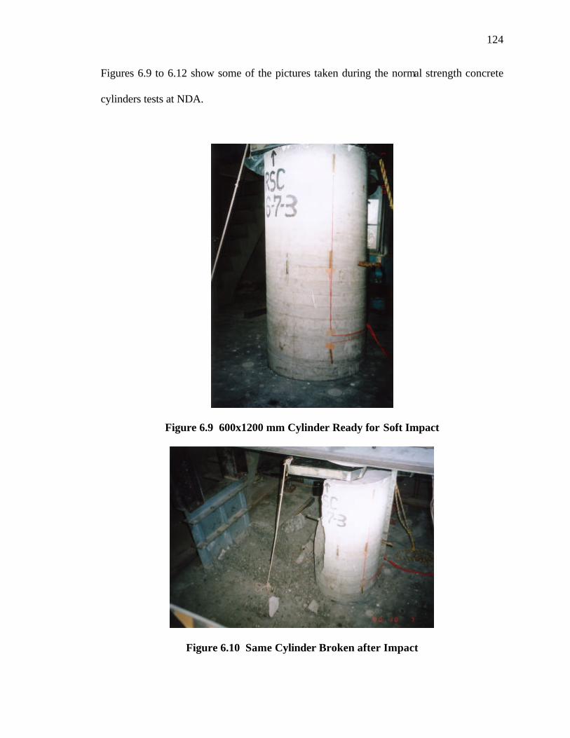
124
Figures 6.9 to 6.12 show some of the pictures taken during the normal strength concrete
cylinders tests at NDA.
Figure 6.9 600x1200 mm Cylinder Ready for Soft Impact
Figure 6.10 Same Cylinder Broken after Impact

125
Figure 6.11 Vertical Splitting Failure Observed
Figure 6.12 A Split Wedge From Inside

126
6.2.2.3 Dynamic Tests Performed at UBC, Canada
All the impact tests on the 3x6 inch (75x150) mm cylinders were carried at the University
of British Colombia, Canada using the heavier of its two drop hammers which weighs
578 kg. Additional tests were carried using the lighter weight hammer which weighs
only 183 kg. Some additional tests were carried on 6x12 inch (150x300 mm) specimens
using both hammers to check on the energy effect on failure of these cylinders. Figures
6.13 and 6.14 show pictures of some of the tests carried out at UBC.
(a) Before Test (b) After Test
Figure 6.13 Soft Impact on a 75x150 mm Specimen at UBC

127
(a) Before Test (b) After Test
Figure 6.14 Hard Impact on a 150x300 mm Specimen at UBC
The results of the tests carried out at UBC are summarized in tables 6.12 and 6.13. Due
to the small size of the specimens, only three strain gages were used. The gages were
placed at the center of the specimen and at 1200 to each other.
Table 6.12 show the maximum stresses obtained during the tests and the corresponding
central strains, while Table 6.13 show the maximum strains obtained at the specimen
center and the corresponding stresses.

128
Table 6.12 UBC Results – Maximum Stresses and Corresponding Strains
Hammer Type
Specimen size
Impact Velocity
Max. stress ( N/mm2)
Time at max. stress (sec)
Strain at max. stress ( µ)
5H1 74.40 0.01024 5715.6 5H2 60.35 0.01024 3679.3 5H3 73.50 0.01028 -11131.1 5S1 128.38 0.01192 285.9 5S2 138.64 0.01206 2559.2 5S3 99.20 0.01156 262.2 7H1 56.47 0.01024 2135.9 7H2 65.14 0.01022 -14949.5 7S1 198.39 0.01148 -12526.1 7S2 98.70 0.01124 -6982.6
3" X 6"
7S3 106.47 0.01078 -27744.1 5H61 112.32 0.01084 1287.5 5H62 135.67 0.01098 13104.3 7H61 105.40 0.0107 -9887.8
Heavy Hammer
6" X 12"
7H62 135.67 0.01098 13104.3 5LH1 51.99 0.01016 13567.2 5LH2 66.53 0.01022 11578.2 5LS1 120.51 0.0128 1325.4 5LS12 165.33 0.01248 -10061.6 5LS13 124.00 0.01202 -13303.3 7LH1 49.60 0.01016 -1756.7 7LH2 68.02 0.0102 -18124.8 7lS1 151.19 0.01286 1786.7
7LS12 157.96 0.01264 2003.2
Light Hammer 3" X 6"
7LS13 140.03 0.01228 11570.3 Conversion factor: 1 MPa (N/mm2) = 145 psi

129
Table 6.13 UBC Results – Maximum Strains and Corresponding Stresses
Hammer Type
Specimen size
Impact Velocity
Time at max. strain
(sec)
Max. strain ( µ)
Stress at max. strain
( N/mm2) 5H1 0.01022 10513.314 40.21 5H2 0.0092 9.7603714 62.71 5H3 0.01004 33.563726 27.55 5S1 0.01184 125.49049 15.85 5S2 0.01282 81.270031 118.63 5S3 0.0118 94.815037 73.78 7H1 0.01012 45.216414 69.84 7H2 0.00996 18.425191 64.26 7S1 0.0122 94.317058 70.84 7S2 0.01104 88.540512 56.55
3" X 6"
7S3 0.01038 90.432829 20.43 5H61 0.01022 72.505616 67.58 5H62 0.0092 9.7603714 40.11 7H61 0.0105 34.460087 75.12
Heavy Hammer
6" X 12"
7H62 0.0106 44.718436 155.91 5LH1 0.01004 33.563726 27.55 5LH2 0.01184 125.49049 15.85 5LS1 0.01282 81.270031 118.63 5LS12 0.0118 94.815037 73.78 5LS13 0.00014 -13696.69 69.84 7LH1 0.00996 18.425191 64.26 7LH2 0.01292 151.18616 12.38 7lS1 0.0127 157.95866 13.83
7LS12 0.0127 157.95866 13.83
Light Hammer 3" X 6"
7LS13 0.01268 128.37876 238.80 Conversion factor: 1 MPa (N/mm2) = 145 psi

130
6.3 Study of Tests Results
From the static test results, and following the calculation procedure outlined in Chapter
Two and detailed by Equations 2.10 and 2.11, the value of d0 was calculated to be 906.6
mm and Bft was found to be 51.69 N/mm2. Figure 6.15 shows a plot of the static size
results and the theoretical static results calculated using the Size Effect law. These
curves were plotted in logarithmic scale for comparison with Bazant’s Size Effect curve.
To understand Figures 6.15, we calculate the logarithm of the diameter for each cylinder
(e.g. 1.875 is the log for 75mm), and the Y-axis value gives the corresponding
logarithmic strength for each point on the curves. From this figure it can be seen clearly
that the Size Effect law represented accurately the static data.
1.2
1.3
1.4
1.5
1.6
1.7
1.8
1.8 2 2.2 2.4 2.6 2.8 3
Log (Size (mm))
Lo
g (
Str
eng
th (
MP
a))
Static ResultsTheoretical Static
Figure 6.15 Size Effect Curves for Static Tests and Theoretical Static Results

131
Figures 6.16 and 6.17 show the results of the hard and soft impact tests for both the 5 m/s
and 7m/s impact velocities plotted together with the static tests results and the theoretical
static results. The dotted part of the series line implies that values are obtained from tests
performed at different locations.
The strength value obtained with the 7 m/s hard impact tests of the 3 x 6 inch (75x150
mm) and the 6x12 inch (150x300 mm) cylinder is lower than the value for the 5 m/s hard
impact (Figure 6.16). This may be due to the fact that the 7 m/s impact produced very
high energies that shattered those cylinders at stress levels lower than the expected
values. This “overwhelming” phenomenon was observed also in the results of the high-
strength concrete tests for the 75x150 cylinders and at the NDA tests of the normal-
strength 300x600 mm cylinders.
0
10
20
30
40
50
60
70
80
0 100 200 300 400 500 600 700Size (mm)
Max
Str
ess
(psi
)
Static ResultsTheoretical Static5 m/s Test Results
7 m/s Test Results
Figure 6.16 Hard Impact Tests

132
0
20
40
60
80
100
120
140
160
0.00 100.00 200.00 300.00 400.00 500.00 600.00 700.00Size (mm)
Max
Str
ess
(psi
)
Static ResultsTheoretical Static
5 m/s Test Results7 m/s Test Results
Figure 6.17 Soft Impact Tests
The overwhelming phenomenon was not observed in the soft impact results except may
be for the 3x6 inch (75x150 mm cylinders). The 5 m/s and 7m/s soft impact results for
this size were very close, as can be seen in Figure 6.17. The very high values obtained
for the 3x6 inch (75x150 mm) cylinders, tested at UBC, are doubtful. The results are
more than twice the static strength of the specimens which makes them too high to
believe. Problems associated with the data acquisition system used at UBC may hint the
unreliability of these values.
From the above figures, it is very clear that a Size Effect phenomenon existed for the
normal-strength cylinder under static loads, hard impact, and soft impact.

133
6.4 Comparison of Test and Pre-Test Simulation Results
The observations from the pre-test finite element simulations and the tests are shown in
Figures 6.18 through 6.21. In these Figures, the logarithm of strength (in MPa.) is plotted
against the logarithm of the specimen size (in mm) for the following cases: 1)
Experimental results obtained for an impact velocity of 7 m/s; 2) Experimental results for
an impact velocity of 5m/s; 3) Static test results; 4) Theoretical static results calculated
using Bazant’s Size Effect law; 5) Pre-test results obtained using the finite element
simulation for an impact velocity of 10 m/s; 6) Pre-test results obtained using the finite
element simulation for an impact velocity of 5 m/s; and 7) Pre-test results obtained using
the finite element simulation for an impact velocity of 1 m/s. Since the results of the
simulations that included strain rate effects and those that did not include strain rate
effects were almost the same, only the results of the simulations with strain rate effects
are presented and discussed.
Figures 6.18 and 6.19 show the hard impact tests results obtained with 7 m/s and 5 m/s
impact velocities compared to the results of the pre-test simulations using the Drucker-
Prager Plasticity Model and the Brittle Fracture Model respectively.
Figures 6.20 and 6.21 show the soft impact tests results for both the 7 m/s and the 5 m/s
impact velocities compared to the results of the pre-test simulations results obtained using
the Drucker-Prager Plasticity Model and the Brittle Fracture Model respectively.

134
0
0.2
0.4
0.6
0.8
1
1.2
1.4
1.6
1.8
2
1.8 2 2.2 2.4 2.6 2.8 3
Log (Diameter (mm))
Lo
g (
Str
eng
th (
MP
a))
STATIC TEST RESULT
THEORETICAL STATIC
5 m/s IMPACT
7 m/s IMPACT
Pre-test FEM, 10 m/s Impact Druker-Prager Plasticity ModelPre-test FEM 5m/s Impact, Druker-PragerPlasticity ModelPre-test FEM 1m/s Impact, Druker-PragerPlasticity Model
Figure 6.18 Hard Impact Size Effect Curves; Pre-Test Simulations with Drucker-
Prager Cap Plasticity Model Compared to Test Results
0
0.5
1
1.5
2
2.5
1.8 2 2.2 2.4 2.6 2.8 3
Log (Diameter (mm))
Lo
g (
Str
eng
th (
MP
a))
STATIC TEST RESULT
THEORETICAL STATIC
5 m/s IMPACT
7 m/s IMPACT
Pre-test FEM 10 m/s Impact, BrittleFracture ModelPre-test FEM 5m/s Impact, Brittle FractureModelPre-test FEM 1m/s Impact, Brittle FractureModel
Figure 6.19 Hard Impact Size Effect Curves; Pre-Test Simulations with the Brittle
Fracture Model Compared to Test Results

135
0
0.5
1
1.5
2
2.5
1.8 2 2.2 2.4 2.6 2.8 3
Log (Diameter (mm))
Log (S
tren
gth
(MP
a))
STATIC TEST RESULT
THEORETICAL STATIC
5 m/s IMPACT
7 m/s IMPACT
Pre-test FEM, 10 m/s Impact Druker-Prager Plasticity ModelPre-test FEM 5m/s Impact, Druker-PragerPlasticity ModelPre-test FEM 1m/s Impact, Druker-PragerPlasticity Model
Figure 6.20 Soft Impact Size Effect Curves; Pre-Test Simulations with Drucker-
Prager Cap Plasticity Model Compared to Test Results
0
0.5
1
1.5
2
2.5
1.8 2 2.2 2.4 2.6 2.8 3
Log (Diameter (mm))
Log (S
tren
gth
(MP
a))
STATIC TEST RESULT
THEORETICAL STATIC
5 m/s IMPACT
7 m/s IMPACT
Pre-test FEM 5m/s Impact, Brittle FractureModelPre-test FEM 10 m/s Impact, BrittleFracture ModelPre-test FEM 1m/s Impact, Brittle FractureModel
Figure 6.21 Soft Impact Size Effect Curves; Pre-Test Simulations with the Brittle
Fracture Model Compared to Test Results

136
The following observations can be made from the comparison of the pre-test and test
results:
• These data indicate that a Size Effect existed for compressively loaded normal-
strength concrete cylinders under both static and dynamic loads. Generally, as the
size of the specimen increased, the apparent strength of the concrete decreased.
• A variation of concrete strength with the variation of the loading rate was observed.
Although this phenomenon has been observed and discussed in abundance, it can be
stated that the results provide more data that can add to that data base.
• The static loading curve and the theoretical curve were almost similar.
• The concrete strength values recorded when the impact velocity was 7 m/s were
higher than the values recorded when the impact velocity was 5 m/s and the static
test values for all sizes of concrete cylinders except for the hard impact strength of
the 6x12 inch (150x300 mm) size. However, the strength values obtained for the 5
m/s impact were lower than the static test strength values for all cylinder sizes,
except for the 75x150 mm size and for the hard impact results of the 150x300 mm
cylinder. This may be due to the conflicting actions of the Size Effect phenomenon
and the loading rate phenomenon. This observation needs to be studied further.
• The results of the 150x300 mm cylinder were considerably below the expected
values (compared with the trend of the data curve). This may be due to the fact that
the energies associated with the impact with the large drop hammer used at Penn
State University were very high for this small cylinder size to withstand and the
cylinder may have shattered at stress values lower than the actual strength. This drop

137
was not observed when the same specimen size was tested at UBC with the smaller
size hammer.
• Generally, the pre-test simulation results differed significantly from the test results.
• All the pre-test simulations were done using the Penn State hammer shape and
dimensions, while the tests were performed at three different locations using three
different hammers with different weights and dimensions.
• The tests were done with impact speeds of 5 m/s and 7 m/s, while the pre-test
simulations used impact speeds of 1 m/s, 5 m/s, and 10 m/s. This change was made
since the 10 m/s velocity could not be achieved with the current setup in all three
places, while the 1 m/s velocity was found to be too low to break the big cylinders.
• The pre-test simulation results obtained using the Drucker-Prager Cap Plasticity
model for concrete differed significantly from the results obtained using the Concrete
Brittle Fracture model.
• Pre-test simulations of the hard impact tests gave better results than the simulations
of the soft impact tests. This is due to the complexities involved with modeling the
hyper-elastic properties of the rubber pads.
The obvious difference between the test results and the pre-test simulations showed that
one had to perform post-test finite element simulations to correct the parameters that may
have contributed to these differences.
138
6.5 Post-test simulations
After completion of the tests, the results obtained using Drucker-Prager Plasticity model
as well as the Brittle Fracture model, were compared with the results obtained from the
impact tests at 5 m/s and 7 m/s model. A significant difference was found between the
two. This difference between the test results and the pre-test simulations showed that one
had to perform post-test finite element simulations to correct the parameters that may
have contributed to these differences.
Bearing in mind the differences between the Penn State (PSU) test setup used in the pre-
test simulations and the actual setup used in the tests at the three different locations, the
finite element model was modified to match the actual test setup at the NDA, UBC, and
even at PSU. Changes were made to the hammer shape and its dimensions to match
those at the NDA and UBC. The impact interface conditions such as the shape and
dimensions of the impacting plate, the thickness of the rubber pad, were changed from
those used in the pre-test simulations to match the ones that were actually used during the
tests at the three different places. A different impacting plate size was used at NDA for
each different cylinder size, while the load cell itself was used to impact the specimen at
UBC. The 10 m/s impact velocity was replaced with the actually used 7 m/s velocity,
while the 5 m/s velocity was kept.
The concrete models parameters were modified using the results from the static tests.
Since no difference was found in the pre-test simulation results between those obtained
with including using strain rate dependent model and those obtained without including

139
strain rate effects in the model, only the strain rate dependent model was used for the
post-test simulations and the related analysis and discussion.
6.5.1 Results of Post-Test simulations of Penn State Tests
6.5.1.1 Hard Impact Tests
Tables 6.14 and 6.15 show the results of the post-test simulations of the hard impact tests
performed at Penn State University (PSU). Table 6.14 shows the maximum stresses
obtained and the corresponding strains, while Table 6.15 shows the maximum strains and
the corresponding stresses.
Table 6.14 Simulation of Penn State Hard Impact Tests – Maximum Stresses
Strain Rate
Effect
Material Model
Impact Velocity
Model Dimension
Max. stress
(N/mm2)
Time at max
stress (s)
strain at maximum
stress
150x300 51.2 2.25E-02 6.43E-01 300x600 44.8 3.90E-03 3.09E-02 7 m/s 600x1200 35.6 1.50E-03 1.04E-03 150x300 52.5 2.70E-02 3.52E-01 300x600 43.8 9.00E-03 1.98E-02
Drucker-Prager
5 m/s 600x1200 24.4 6.75E-03 1.60E-03 150x300 22.5 6.75E-03 1.23E-02 300x600 43.3 3.01E-04 1.39E-03 7 m/s 600x1200 33.3 2.25E-03 1.02E-03 150x300 47.9 7.51E-04 1.55E-03 300x600 35.6 3.00E-03 2.00E-03
Yes
Brittle Fracture
5 m/s
600x1200 25.3 2.25E-03 7.72E-04 Conversion factor: 1 MPa (N/mm2) = 145 psi

140
Table 6.15 Simulation of Penn State Hard Impact Tests – Maximum Strains
Strain Rate
Effect
Material Model
Impact Velocity
Model Dimension
Max. strain
Time at max strain
(ms)
stress at maximum
strain (N/mm2)
150x300 -6.43E-01 2.25E-02 51.2 300x600 -7.438E-03 3.01E-04 11.9 7 m/s 600x1200 -1.91E+04 1.50E-03 4.5 150x300 -4.12E-01 3.00E-02 5.5 300x600 -2.36E-02 9.75E-03 0.1
Drucker-Prager
5 m/s 600x1200 -2.25E-02 6.75E-03 7.3 150x300 1.23E-02 6.75E-03 22.5 300x600 1.39E-03 3.01E-04 43.3 7 m/s 600x1200 1.02E-03 2.25E-03 33.3 150x300 1.55E-03 7.51E-04 47.9 300x600 2.000E-03 3.00E-03 35.6
Yes
Brittle Fracture
5 m/s 600x1200 7.72E-04 2.25E-03 25.3
Conversion factor: 1 MPa (N/mm2) = 145 psi
6.5.1.2 Soft Impact Tests
Tables 6.14 and 6.15 show the results of the post-test simulations of the soft impact tests
performed at Penn State University (PSU). Table 6.14 shows the maximum stresses
obtained and the corresponding strains, while Table 6.15 shows the maximum strains and
the corresponding stresses.

141
Table 6.16 Simulation of Penn State Soft Impact Tests – Maximum Stresses
Strain Rate
Effect
Material Model
Impact Velocity
Model Dimension
Max. stress
Time at max stress
(ms)
strain at maximum
stress
150x300 18.9 2.60E-03 -1.31E-03 300x600 25.6 3.90E-03 -9.67E-02
7 m/s
600x1200 25.4 9.00E-03 -1.78E-03 150x300 13.8 2.80E-03 -5.09E-04 300x600 22.9 3.90E-03 -1.18E-03
Drucker-Prager
5 m/s 600x1200 21.4 5.70E-03 -8.83E-04 150x300 27.2 2.50E-03 -8.31E-04 300x600 49.3 3.00E-03 -1.66E-03 7 m/s 600x1200 25.6 3.60E-03 -7.82E-04 150x300 15.5 2.80E-03 -4.55E-04 300x600 28.6 3.30E-03 -9.80E-04
Yes
Brittle Fracture
5 m/s 600x1200 19.3 4.20E-03 -6.66E-04
Table 6.17 Simulation of Penn State Soft Impact Tests – Maximum Strains
Strain Rate
Effect
Material Model
Impact Velocity
Model Dimension Max. strain
Time at max strain
(ms)
stress at maximum
strain
150x300 -5.44E-02 2.60E-03 18.9 300x600 -9.67E-02 3.90E-03 25.6 7 m/s 600x1200 -6.48E-02 1.04E-02 7.4 150x300 -2.14E-02 2.80E-03 13.8 300x600 -5.66E-02 3.98E-03 10.0
Drucker-Prager
5 m/s 600x1200 -3.66E-02 7.50E-03 7.9 150x300 -8.31E-04 2.50E-03 27.2 300x600 -1.66E-03 3.00E-03 49.3 7 m/s 600x1200 -8.78E-04 3.60E-03 25.8 150x300 -4.55E-04 2.80E-03 15.5 300x600 -9.80E-04 3.30E-03 28.6
Yes
Brittle Fracture
5 m/s 600x1200 -6.66E-04 4.20E-03 19.3
Conversion factor: 1 MPa (N/mm2) = 145 psi

142
6.5.2 Results of Post-Test simulations of NDA Tests
6.5.2.1 Hard Impact Tests
Tables 6.18 and 6.19 show the results of the post-test simulations of the hard impact tests
performed at National Defense Academy in Japan (NDA). Table 6.18 shows the
maximum stresses obtained and the corresponding strains, while Table 6.19 shows the
maximum strains and the corresponding stresses.
Table 6.18 Simulation of NDA Hard Impact Tests – Maximum Stresses
Strain Rate
Effect
Material Model
Impact Velocity
Model Dimension
Max. Stress
(N/mm2)
Time at max stress
(ms)
strain at maximum
stress
300x600 18.7 1.53E-04 -1.19E-03 7 m/s
600x1200 35.6 1.50E-03 1.04E-03 300x600 17.6 1.52E-04 -9.43E-04
Drucker-Prager
5 m/s 600x1200 24.4 6.75E-03 1.60E-03 300x600 25.6 1.65E-03 -7.87E-04
7 m/s 600x1200 32.4 2.25E-03 1.02E-03 300x600 17.0 1.51E-04 -5.14E-04
Yes
Brittle Fracture
5 m/s 600x1200 25.3 2.25E-03 -5.14E-04
Table 6.19 Simulation of NDA Hard Impact Tests – Maximum Strains
Strain Rate
Effect
Material Model
Impact Velocity
Model Dimension
Max. strain Time at
max strain (ms)
stress at maximum
strain
300x600 -1.498E-03 9.00E-04 7.5 7 m/s
600x1200 -1.91E+04 1.50E-03 4.5 300x600 -9.47E-04 4.52E-04 9.0
Drucker-Prager
5 m/s 600x1200 -2.25E-02 6.75E-03 7.3 300x600 -7.87E-04 1.65E-03 25.6
7 m/s 600x1200 1.02E-03 2.25E-03 33.3 300x600 -5.140E-04 1.51E-04 17.0
Yes
Brittle Fracture
5 m/s 600x1200 7.72E-04 2.25E-03 25.3

143
6.5.2.2 Soft Impact Tests
Tables 6.20 and 6.21 show the results of the post-test simulations of the soft impact tests
performed at the National Defense Academy, Japan (NDA). Table 6.20 shows the
maximum stresses obtained and the corresponding strains, while Table 6.21 shows the
maximum strains and the corresponding stresses.
Table 6.20 Simulation of NDA Soft Impact Tests – Maximum Stresses
Strain Rate
Effect
Material Model
Impact Velocity
Model Dimension
Max. stress
Time at max stress (ms)
strain at maximum
stress
300x600 25.6 3.90E-03 -9.67E-02 7 m/s
600x1200 25.4 9.00E-03 -1.78E-03 300x600 22.9 3.90E-03 -1.18E-03
Drucker-Prager
5 m/s 600x1200 21.4 5.70E-03 -8.83E-04 300x600 49.3 3.00E-03 -1.66E-03
7 m/s 600x1200 25.6 3.60E-03 -7.82E-04 300x600 28.6 3.30E-03 -9.80E-04
Yes
Brittle Fracture
5 m/s 600x1200 19.3 4.20E-03 -6.66E-04
Table 6.21 Simulation of NDA Soft Impact Tests – Maximum Strains
Strain Rate
Effect
Material Model
Impact Velocity
Model Dimension Max. strain
Time at max strain
(ms)
stress at maximum
strain
300x600 -9.67E-02 3.90E-03 25.6 7 m/s
600x1200 -6.48E-02 1.04E-02 7.4 300x600 -5.66E-02 3.98E-03 10.0
Drucker-Prager
5 m/s 600x1200 -3.66E-02 7.50E-03 7.9 300x600 -1.66E-03 3.00E-03 49.3
7 m/s 600x1200 -8.78E-04 3.60E-03 25.8 300x600 -9.80E-04 3.30E-03 28.6
Yes
Brittle Fracture
5 m/s 600x1200 -6.66E-04 4.20E-03 19.3
Conversion factor: 1 MPa (N/mm2) = 145 psi

144
6.5.3 Results of Post-Test simulations of UBC Tests
Tables 6.22 and 6.23 show the results of the post-test simulations of the hard impact tests
performed at the University of British Colombia (UBC). Table 6.22 show the maximum
stresses obtained and the corresponding strains for both the hard and soft impacts, while
Table 6.23 shows the maximum strains and the corresponding stresses for both the hard
and soft impacts.
Table 6.22 Simulation of UBC Impact Tests – Maximum Stresses
Model size
(mm)
Strain Rate
Effect
Impact Interface
Material Model
Impact Velocity
Max. stress
(N/mm2)
Time at max stress
(s)
strain at maximum
stress
5 m/s 25.6 3.90E-03 -9.67E-02 Drucker Prager 7 m/s 25.4 9.00E-03 -1.78E-03
5 m/s 22.9 3.90E-03 -1.18E-03 Hard
Brittle Fracture 7 m/s 21.4 5.70E-03 -8.83E-04
5 m/s 49.3 3.00E-03 -1.66E-03 Drucker Prager 7 m/s 25.6 3.60E-03 -7.82E-04
5 m/s 28.6 3.30E-03 -9.80E-04
75x150 Yes
Soft Brittle
Fracture 7 m/s 19.3 4.20E-03 -6.66E-04
Table 6.23 Simulation of UBC Impact Tests – Maximum Strains
Model size
(mm)
Strain Rate
Effect
Impact Interface
Material Model
Impact Velocity
Max. strain
Time at max strain
(ms)
stress at maximum
strain
5 m/s -9.67E-02 3.90E-03 25.6 Drucker Prager 7 m/s -6.48E-02 1.04E-02 7.4
5 m/s -5.66E-02 3.98E-03 10.0 Hard
Brittle Fracture 7 m/s -3.66E-02 7.50E-03 7.9
5 m/s -1.66E-03 3.00E-03 49.3 Drucker Prager 7 m/s -8.78E-04 3.60E-03 25.8
5 m/s -9.80E-04 3.30E-03 28.6
75x150 Yes
Soft Brittle
Fracture 7 m/s -6.66E-04 4.20E-03 19.3

145
6.6 Summary of Results
The observations from the post-test finite element simulations and the tests are shown in
Figures 6.18 through 6.21. In these Figures, the logarithm of strength (in MPa.) is plotted
against the logarithm of the specimen size (in mm) for the following cases:
1. Experimental results obtained for an impact velocity of 7 m/s.
2. Experimental results for an impact velocity of 5m/s.
3. Static test results.
4. Results calculated using Bazant’s Size Effect law3.
5. Post-test results obtained using the finite element simulation for an impact
velocity of 5 m/s.
6. Post-test results obtained using the finite element simulation for an impact
velocity of 7 m/s.
Figures 6.18 and 6.19 show the hard impact tests results obtained with 7 m/s and 5 m/s
impact velocities compared to the results of the post-test simulations using the Drucker-
Prager Plasticity Model and the Brittle Fracture Model respectively.
Figures 6.20 and 6.21 show the soft impact tests results for both the 7 m/s and the 5 m/s
impact velocities compared to the results of the post-test simulations results obtained
using the Drucker-Prager Plasticity Model and the Brittle Fracture Model respectively.

146
1.2
1.3
1.4
1.5
1.6
1.7
1.8
1.9
1.8 2 2.2 2.4 2.6 2.8 3
Log (Size (mm))
Lo
g (
Str
eng
th (
MP
a))
Static Results5 m/s Test Results5 m/s Druker-Prager ModelTheoretical Static7 m/s Test Results7 m/s Druker-Prager Model
Figure 6.22 Hard Impact Size Effect Curves; Post Test Simulations with Drucker-
Prager Cap Plasticity Model Compared to Test Results
1.2
1.3
1.4
1.5
1.6
1.7
1.8
1.9
1.8 2 2.2 2.4 2.6 2.8 3
Log (Size (mm))
Log
(Str
engt
h (M
Pa)
)
Static ResultsTheoretical Static7 m/s Brittle Fracture Model7 m/s Test Results5 m/s Brittle Fracture Model5 m/s Test Results
Figure 6.23 Hard Impact Size Effect Curves; Post Test Simulations with the Brittle
Fracture Model Compared to Test Results

147
0
0.5
1
1.5
2
2.5
1.80 2.00 2.20 2.40 2.60 2.80 3.00
Log (Size (mm))
Lo
g (
Str
eng
th (
MP
a))
Static ResultsTheoretical Static5 m/s Test Results7 m/s Test Results5 m/s Druker-Prager Model7 m/s Druker-Prager Model
Figure 6.24 Soft Impact Size Effect Curves; Post Test Simulations with Drucker-
Prager Cap Plasticity Model Compared to Test Results
0
0.5
1
1.5
2
2.5
1.80 2.00 2.20 2.40 2.60 2.80 3.00
Log (Size (mm))
Lo
g (
Str
eng
th (
MP
a))
Static ResultsTheoretical Static5 m/s Test Results7 m/s Test Results5 m/s Brittle Fracture Model7 m/s Brittle Fracture Model
Figure 6.25 Soft Impact Size Effect Curves; Post Test Simulations with the Brittle
Fracture Model Compared to Test Results

148
6.7 Discussion of Results
The following observations can be made from the above figures:
• These data indicate that a Size Effect existed for compressively loaded normal-
strength concrete cylinders under both static and dynamic loads. Generally, as the
size of the specimen increased, the apparent strength of the concrete decreased.
• A variation of concrete strength with the variation of the loading rate was observed.
Although this phenomenon has been observed and discussed in abundance, it can be
stated that the results provide more data that can add to that data base.
• The static loading curve and the theoretical curve were almost similar.
• The concrete strength values recorded when the impact velocity was 7 m/s were
higher than the values recorded when the impact velocity was 5 m/s and the static
test values for all sizes of concrete cylinders except for the hard impact strength of
the 6x12 inch (150x300 mm) size. However, the strength values obtained for the 5
m/s impact were lower than the static test strength values for all cylinder sizes,
except for the 75x150 mm size and for the hard impact results of the 150x300 mm
cylinder. This may be due to the conflicting actions of the Size Effect phenomenon
and the loading rate phenomenon. This observation needs to be studied further.
• The results of the 150x300 mm cylinder were considerably below the expected
values (compare with the trend of the data curve). This may be due to the fact that
the energies associated with the impact with the large drop hammer used at Penn
State University were very high for this small cylinder size to withstand and the
cylinder may have shattered at stress values lower than the actual strength. This drop

149
was not observed when the same specimen size was tested at UBC with the smaller
size hammer.
• Both post-test finite element models succeeded in predicting the existence of a Size
Effect phenomenon.
• The post-test finite element simulations of the hard impact tests with the Drucker-
Prager plasticity model were almost similar to the test results for all sizes except for
the overwhelmed result of the 7 m/s impact on the 150x300 mm cylinder size. The
simulations using the Brittle Fracture Model are also very close to the test results but
not as close as the results of the Drucker-Prager Model. However, the Brittle
Fracture Model succeeded in modeling the overwhelmed result of the 7 m/s impact
on the 150x300 mm cylinder.
• The post-test simulations of the soft impact tests were not as close to the test results
as the simulations of the hard impact tests. The may be due to the difficulty of
modeling the hyper-elastic properties of the rubber pad.
• Both models succeeded in predicting the strain rate effects, i.e. that the strength
values with a 7 m/s impact speed would be higher than the strength values with a 5
m/s impact speed.
• Concrete strength values obtained in hard impact tests were generally higher than
those obtained in soft impact tests.
6.8 Summary of main achievements
1. Existence of size Effect was proved for normal-strength concrete cylinders under both
static and dynamic axial compressive loads.

150
2. The Size Effect law predictions were proved to match the static test results for the
normal-strength concrete specimens.
3. Higher loading rates were found to enhance the apparent strength of normal-strength
concrete specimens.
4. Two finite element models were developed using ABAQUS EXPLICIT version 6.2.
The first is a modified Drucker-Prager Cap Plasticity model; the second is a Brittle
Fracture model. Both post-test finite element models, which were fine-tuned using
the results of the static tests for each cylinder size, succeeded in predicting the
existence of a Size Effect phenomenon. The Drucker-Prager model predictions
almost matched the impact test results especially the hard impact test results. The
Brittle Fracture model results were less accurate, but agreed with the impact tests
within acceptable limits.

151
CHAPTER SEVEN
RESULTS AND DISCUSSION – COMPARISON OF
NORMAL-STRENGTH AND HIGH-STRENGTH CONCRETE RESULTS
In this chapter, the results of the tests and the simulation for the normal strength and the
high-strength concrete cylinders are compared to each other. Comparison includes both,
the results obtained in the static domain and the results obtained in the dynamic domain.
7.1 Static Test Results
The results of both the high-strength and the normal-strength concrete cylinders are
compared in terms of many different aspects such as the success of the Size Effect law in
representing the data; and the existence of a Size Effect for the modulus of elasticity of
concrete and the strain at maximum stress.
7.1.1 Static Tests Data and the Size Effect Law
For both types of concrete, the Size Effect law managed to almost represent the static test
data exactly. Figure 7.1 show the static test data for the high-strength concrete cylinders
plotted with the values computed us ing the Size Effect law.

152
Normal Strength Concrete
11.11.21.31.41.51.61.71.8
1.8 2.3 2.8
log (diameter (mm))
log
(str
engt
h (M
Pa)
)
Static Tests
Size Effect Law
Figure 7.1 Static Test Data and the Size Effect Law for Normal and High-Strength
Concrete Cylinders
From the above figures, it is clear that the high-strength concrete curve is much steeper
than the normal strength concrete curve and the difference in strength between the bigger
sizes and the smaller sizes is larger for the high-strength concrete than it is for the normal
strength concrete. This is due to the fact that d0 (the diameter of the size at which the
failure mode changes from plasticity to fracture mechanics) for the normal strength
High-Strength Concrete
1.7 1.75 1.8
1.85 1.9
1.95 2
1.8 2.3 2.8
log (diameter (mm))
log
(str
engt
h (M
Pa)
) Static Test
Size Effect Law

153
concrete has a value of 906.64 mm. This value is greater than the diameter of the biggest
cylinder size (600 mm). This means that all the normal strength concrete specimens lay
in the plasticity region in the Size Effect curve presented in Figure 2.1 in Chapter two.
For the high-strength concrete, do is equal to 268.93 mm which means that the two
smaller cylinder sizes fail under a different mode of failure than the two bigger sizes and
the two bigger sizes lay in the fracture mechanics part of the Size Effect curve.
Table 7.1 Static Strength Values for High-Strength Concrete Cylinders Compared
to Size Effect Law Values
Specimen Size
H
(mm)
D
(mm)
Static Test
Results
(MPa)
Size Effect Law
Results
(MPa)
Percentage
Difference
%
150 75 89.46 91.45 2
300 150 82.86 82.86 0
600 300 71.1 71.1 0
1200 600 57.53 57.53 0
Conversion factor: 1 MPa (N/mm2) = 145 psi

154
Table 7.2 Static Strength Values for Normal-Strength Concrete Cylinders
Compared to Size Effect Law Values
Specimen Size
H
(mm)
D
(mm)
Static Test
Results
(MPa)
Size Effect Law
Results
(MPa)
Percentage
Difference
%
150 75 42.58* 49.60 1.64
300 150 47.88 47.88 0
600 300 44.81 44.81 0
1200 600 40.10 40.10 0
Conversion factor: 1 MPa (N/mm2) = 145 psi
7.1.2 Modulus of Elasticity
A variation of the modulus of elasticity with the variation of size was observed for both
the high-strength and the normal-strength concrete. This contradicts the results obtained
by Baalbaki et al. (1992). However the drop in the modulus of elasticity of the smaller
size specimen may suggest that the results they got were due to the fact that they used
micro-concrete in their tests, and all their specimens are equal to or less than 150 mm in
diameter.
In Figure 7.2, the modulus of elasticity for both the normal and the high-strength concrete
was plotted in a logarithmic curve similar to that of the Size Effect curve. The shapes
obtained look similar to the strength curves and may suggest that the Size Effect law can
be modified to allow for the calculation of the corresponding modulus of elasticity.

155
Modulus of Elasticity
4.2
4.3
4.4
4.5
4.6
4.7
1.8 2.3 2.8
log (diameter (mm))
log
(E (
MP
a))
High-StrengthConcrete
Normal-StrengthConcrete
Figure 7.2 Variation of Modulus of Elasticity with Size for Normal and High-
Strength Concrete Cylinders
7.1.3 Strain at Maximum Stress
In Figure 7.3, the observed values of strain at maximum stress are plotted against the size
for both the high-strength and the normal-strength concrete.
As can be seen from the two graphs, the high-strength concrete shows a very clear
variation of strain at maximum stress values with the variation of size. However, the
normal-strength concrete does not show the same clear variation, the curve is almost a
horizontal straight line with an expected drop in the observed the value for the 75x150
mm cylinders which was tested 18 month earlier than the rest of the specimens. The
nature of the curve for the normal strength concrete can be explained by the fact that all
the specimens lay in the plasticity zone in the Size Effect curve (since all specimens
diameters are less than the transitional value d0). On the other hand the clear Size Effect

156
in the strain at maximum stress values for the high-strength concrete cylinders may be
explain ed by the fact that the specimens size distribution bridges the gap between
plasticity and fracture mechanics.
0
500
1000
1500
2000
2500
0 200 400 600 800
diameter (mm)
stra
in a
t m
ax. s
tres
s ( µ
)
High-StrengthConcrete
Normal-StrengthConcrete
Figure 7.3 Variation of Strain at Maximum Stress Values with Size for Normal and
High-Strength Concrete Cylinders
7.2 Dynamic Test Results
The results of the hard impact tests on the high-strength concrete cylinders are compared
here with the results of both, the hard and the soft impact tests, on the normal-strength
concrete cylinders. Comparison includes: the modes of failure observed during the tests,

157
and the existence of a Size Effect for the modulus of elasticity of and the strain at
maximum stress.
7.2.1 Modes of Failure
Several modes of failures were observed during the impact tests. The help provided by
the high-speed photography was crucial in enabling the detection of some of these modes.
However, since only one high-speed camera was used, some of the modes of failure listed
below might be the same mode that appeared in a different form when looked at from a
different view angle.
The 600x1200 mm cylinders of both the normal-strength and the high-strength concrete
as well as the 300x600 mm high-strength concrete cylinders experienced primarily a
vertical brittle splitting failure.
Splitting of the 600x1200 mm cylinder size, of both types of concrete, took the shape of
three vertical planes almost at 1200 to each other, as seen on Figures 7.4 and 7.5. Vertical
splitting of the 300x600 mm high-strength concrete cylinders happened in more than one
type: one type is splitting in three planes at 1200 to each other as seen in Figure 7.6-(a).
Another type is a symmetric splitting into two halves (Figure 7.6-b).

158
.
Figure 7.4 Vertical Splitting Failure of NSC 600x1200 mm Cylinder
Figure 7.5 Vertical Splitting Failure of HSC 600x1200 mm Cylinder

159
(a) Three Splitting planes at 1200 (b) Symmetrical Splitting
Figure 7.6 Vertical Splitting Failure of HSC 300x600 mm Cylinders
The 300x600 mm normal strength concrete cylinders and the 150x300 mm and 75x150
mm cylinders of both the normal strength and the high strength concrete experienced
many different failure modes. Some of the observed modes are:
a) Vertical Splitting: in which the cylinder split vertically through two, three, or
more vertical planes. Splitting either started at the top (Figure 7.7 (a)) or at the
bottom of the specimen (Figure 7.7(b)). Some specimens failed under combined
shear and splitting as shown in Figure 7.8.
It was observed that the splitting type of failure was associated with higher levels
of strength. Specimens that failed by this mode of failure recorded the highest
strength among their group. This may indicate that theses specimens crossed the
transitional gap between plasticity and fracture mechanics.
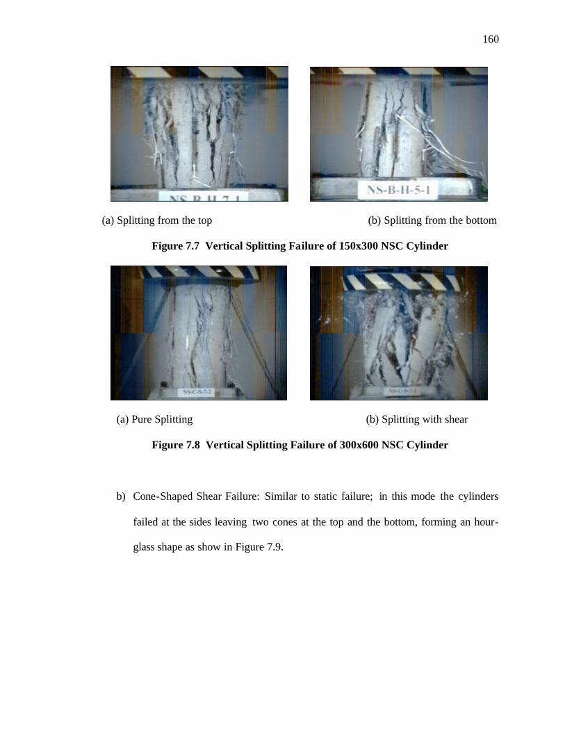
160
(a) Splitting from the top (b) Splitting from the bottom
Figure 7.7 Vertical Splitting Failure of 150x300 NSC Cylinder
(a) Pure Splitting (b) Splitting with shear
Figure 7.8 Vertical Splitting Failure of 300x600 NSC Cylinder
b) Cone-Shaped Shear Failure: Similar to static failure; in this mode the cylinders
failed at the sides leaving two cones at the top and the bottom, forming an hour-
glass shape as show in Figure 7.9.

161
Figure 7.9 Cone Failure of 75x150 mm NSC Cylinders
c) Diagonal Shear Failure: this type is characterized by a diagonal failure plane as
shown in Figure 7.10 (a). Shear failure occurred in some of the specimens
combined with vertical splitting in some cases, as shown in Figure 7.10 (b), and
with shell bursting in some other cases as can be seen in Figure 7.10 (c).
(a) Shear failure (b) Combined shear and splitting

162
(c) Combined shear and shell bursting
Figure 7.10 Shear Failure of NSC Cylinders
d) Buckling failure: this mode of failure was distinguished with the inflation of the
cylinder from the top or the bottom and the bulging of the materials as shown in
Figure 7.11.
(a) Bottom buckling (b) Top buckling
Figure 7.11 Buckling Failure

163
e) Compressive belly failure: Occurred with the inflation of the center of the
cylinder forming a belly shape. In some cases it happened combined with the
shell bursting failure. Figure 7.12 show examples of this type of failure.
Figure 7.12 Compressive Belly Failure of Cylinders
f) Shell-Core failure: happened by bursting of the shell of the cylinder leaving a
core at the centre as shown in Figure 7.13. This failure was accompanied by a
second peak in the load vs time curve as shown in Figure 7.14 (b).
(a) Shell-Core failure of 150x300 mm specimen

164
(b) Shell-Core failure of 300x600 mm specimen
Figure 7.13 Shell-Core Failure of Cylinders
Time (s)
Lo
ad (
kip
)
Time (s)
Acc
eler
atio
n (g
)
(a) Single Peak (b) Double Peak
Figure 7.14 Second Peak associated with Shell-Core Failure

165
g) Progressive collapse: This type of failure was characterized with the gradual
transfer of failure from the top to the bottom of cylinder as the hammer went
deeper down inside the cylinder. The difference between this type of failure and
the other types that may look similar is that in this failure type, the specimen
stands intact in place while the hammer is moving down, and progressively
eroding the specimen from the top. Figures 7.15 and 7.16 show two examples of
the progressive collapse mode of failure. The figures show the eroding progress
of the concrete cylinder at different stages from the beginning of the impact.
(a) At 2.67 ms from start of contact (b) At 6 ms from start of contact
(c) At 14 ms from start of contact
Figure 7.15 Progressive Collapse of Cylinders

166
7.2.2 Strength Criteria
Figures 7.16 and 7.17 show the existence of Size Effect in both the soft impact tests of
the high-strength concrete cylinders, and the soft and hard impact tests of the normal
strength concrete cylinders.
NSC - Hard Impact
1.000
1.200
1.400
1.600
1.800
2 2.2 2.4 2.6 2.8 3
Log (diameter (mm))
log
(str
engt
h (M
Pa)
)
7 m/s Impact
5 m/s ImpactStatic Test
(a) Hard Impact
NSC - Soft Impact
1.00
1.20
1.40
1.60
1.80
2.00 2.20 2.40 2.60 2.80 3.00
log (diameter (mm))
log
(str
engt
h (M
pa))
7 m/s Impact
5 m/s ImpactStatic Test
(b) Soft Impact
Figure 7.16 Size Effect curves for Normal-Strength Concrete Cylinders
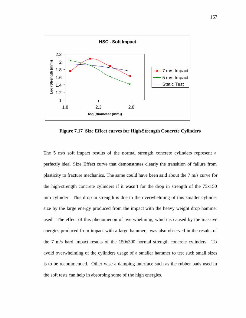
167
HSC - Soft Impact
1
1.2
1.4
1.6
1.8
2
2.2
1.8 2.3 2.8log (diameter (mm))
Log
(Str
engt
h (m
m))
7 m/s Impact
5 m/s ImpactStatic Test
Figure 7.17 Size Effect curves for High-Strength Concrete Cylinders
The 5 m/s soft impact results of the normal strength concrete cylinders represent a
perfectly ideal Size Effect curve that demonstrates clearly the transition of failure from
plasticity to fracture mechanics. The same could have been said about the 7 m/s curve for
the high-strength concrete cylinders if it wasn’t for the drop in strength of the 75x150
mm cylinder. This drop in strength is due to the overwhelming of this smaller cylinder
size by the large energy produced from the impact with the heavy weight drop hammer
used. The effect of this phenomenon of overwhelming, which is caused by the massive
energies produced from impact with a large hammer, was also observed in the results of
the 7 m/s hard impact results of the 150x300 normal strength concrete cylinders. To
avoid overwhelming of the cylinders usage of a smaller hammer to test such small sizes
is to be recommended. Other wise a damping interface such as the rubber pads used in
the soft tests can help in absorbing some of the high energies.

168
7.2.3 Loading Rate Effect
The loading rate effect was very clear in all three sets of results. In Figures 7.16 and 7.17
it is seen that the 7 m/s impact results are higher than the 5m/s impact results for all three
sets. Then only exception happens when the 7 m/s impact overwhelms the specimen, and
the resulting strength is reduced by this effect.
7.2.4 Strains at Maximum Stress
In Figures 7.18 and 7.19 the average values of top, middle, and bottom strains, recorded
at maximum stress values, are plotted against the specimen diameter for both, the soft
impact tests of the high-strength concrete cylinders, and the soft and hard impact tests of
the normal strength concrete cylinders.
The high-strength curves for both, the 5 m/s impact and the 7 m/s impact, display clearly
the variation of strain at maximum stress with the variation of the specimen size.
The normal-strength concrete results show a general trend of variation with size.

169
NSC - 7 m/s Hard Impactstrain at maximum stress
0.00E+00
5.00E-04
1.00E-03
1.50E-03
2.00E-03
2.50E-03
3.00E-03
3.50E-03
4.00E-03
4.50E-03
0 100 200 300 400 500 600 700
Size (mm)
stra
in a
t Max
Str
ess
(µ
ε)
Top strain
Middle Strain
Bott. Strain
(a) 7 m/s Hard Impact
NSC - 5 m/s Hard Impactstrain at maximum stress
0.00E+00
5.00E-04
1.00E-03
1.50E-03
2.00E-03
2.50E-03
3.00E-03
3.50E-03
4.00E-03
4.50E-03
5.00E-03
0 100 200 300 400 500 600 700
Size (mm)
stra
in a
t Max
Str
ess
(µ
ε)
Top strain
Middle Strain
Bott. Strain
(b) 5 m/s Hard Impact

170
NSC - 7 m/s Sof Impactstrain at maximum stress
0.00E+00
5.00E+02
1.00E+03
1.50E+03
2.00E+03
2.50E+03
0.00 100.00 200.00 300.00 400.00 500.00 600.00 700.00
Size (mm)
stra
in a
t Max
Str
ess
(µ
ε)
Top strain
Middle Strain
Bott. Strain
(c) 7 m/s Soft Impact
NSC - 5 m/s Sof Impactstrain at maximum stress
0.00E+00
5.00E+02
1.00E+03
1.50E+03
2.00E+03
2.50E+03
0.00 100.00 200.00 300.00 400.00 500.00 600.00 700.00
Size (mm)
stra
in a
t Max
Str
ess
(µ
ε)
Top strain
Middle Strain
Bott. Strain
(d) 5 m/s Soft Impact
Figure 7.18 Variation of Strain at Max. Stress with Size – Hard and Soft Impact on
Normal Strength Concrete Cylinders

171
HSC - 7 m/s Soft Impactstrain at maximum stress
0
500
1000
1500
2000
2500
0 100 200 300 400 500 600 700
diameter (mm)
Str
ain
(µ
)
Top strain
Midd. strain
Bott. strain
HSC - 5 m/s Soft Impactstrain at maximum stress
0
200
400
600800
1000
1200
1400
1600
0 200 400 600 800
diameter (mm)
Str
ain
(µ
)
Top strain
Midd. strainBott. strain
Figure 7.19 Variation of Strain at Max. Stress with Size - Soft Impact on High-
Strength Concrete Cylinders
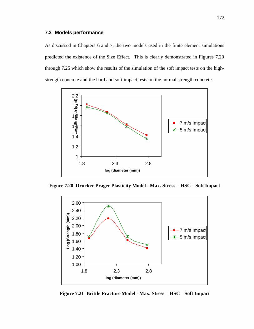
172
7.3 Models performance
As discussed in Chapters 6 and 7, the two models used in the finite element simulations
predicted the existence of the Size Effect. This is clearly demonstrated in Figures 7.20
through 7.25 which show the results of the simulation of the soft impact tests on the high-
strength concrete and the hard and soft impact tests on the normal-strength concrete.
Figure 7.20 Drucker-Prager Plasticity Model - Max. Stress – HSC – Soft Impact
Figure 7.21 Brittle Fracture Model - Max. Stress – HSC – Soft Impact
1
1.2
1.4
1.6
1.8
2
2.2
1.8 2.3 2.8 log (diameter (mm))
Lo
g (S
tren
gth
(mm
))
7 m/s Impact 5 m/s Impact
1.00 1.20
1.40 1.60 1.80
2.00 2.20
2.40 2.60
1.8 2.3 2.8 log (diameter (mm))
Lo
g (S
tren
gth
(mm
))
7 m/s Impact 5 m/s Impact

173
1.00
1.20
1.40
1.60
1.80
2 2.2 2.4 2.6 2.8 3
Size (inch)
Max
Str
ess
(psi
)
7 m/s
5 m/s
Figure 7.22 Drucker-Prager Plasticity Model - Max. Stress – NSC – Hard Impact
1.00
1.20
1.40
1.60
1.80
2 2.2 2.4 2.6 2.8 3
Size (inch)
Max
Str
ess
(psi
)
7 m/s
5 m/s
Figure 7.23 Brittle Fracture Model - Max. Stress – HSC – Hard Impact

174
1.00
1.20
1.40
1.60
2.00 2.20 2.40 2.60 2.80 3.00
Size (inch)
Max
Str
ess
(psi
)
7 m/s
5 m/s
Figure 7.24 Drucker-Prager Plasticity Model - Max. Stress – NSC – Soft Impact
1.00
1.20
1.40
1.60
1.80
2.00 2.20 2.40 2.60 2.80 3.00
Size (inch)
Max
Str
ess
(psi
)
7 m/s
5 m/s
Figure 7.25 Brittle Fracture Model - Max. Stress – NSC – Soft Impact

175
The Drucker-Prager plasticity model results for the hard impact tests of the normal
strength concrete cylinders matched almost exactly the test results. This may be due to
the fact that all the normal strength concrete specimens lay in the plasticity region in the
Size Effect curves. It may be recommended that when modeling concrete tests on
specimens of different size to determine the value of d0 first. Then a plasticity based
model should be used for all the specimens that lie in the plasticity region of the Size
Effect curve and a fracture based model for all the specimens that lie in the fracture part
of the Size Effect curve.
In general the performance of the two models was better in the hard impact tests than in
the soft impact results. This is due to difficulties associated with modeling the hyper-
elastic properties of the rubber pads used in the tests.
The Brittle Fracture model was found to be successful in predicting the drop in strength
of the smaller sizes specimens when overwhelmed by a larger hammer.
Figure 7.26 to 7.31 show the model predictions for the variation of strain at maximum
stress with time. The hard impact normal-strength concrete curves for both, the Drucker-
Prager model and the Brittle Fracture Model, display clearly the variation of strain at
maximum stress with the variation of the specimen size. The high-strength and the
normal-strength concrete soft impact results show a general trend of variation with size
for the two big cylinder sizes. However the results for these soft impacts are affected by
the rubber presence.

176
0
40000
80000
120000
160000
200000
0 100 200 300 400 500 600 700
diameter (mm)
Str
ain
(µ
)
5 m/s
7 m/s
Figure 7.26 Drucker-Prager Plasticity Model – Strain at Max. Stress – HSC – Soft
0
40000
80000
120000
160000
200000
0 100 200 300 400 500 600 700
diameter (mm)
Str
ain
(µ
)
5 m/s
7 m/s
Figure 7.27 Brittle Fracture Model – Strain at Max. Stress – HSC – Soft

177
0.00E+00
1.00E-01
2.00E-01
3.00E-01
4.00E-01
5.00E-01
6.00E-01
7.00E-01
0 100 200 300 400 500 600 700
Size (mm)
stra
in a
t Max
Str
ess
(µ
ε)
7 m/s
5 m/s
Figure 7.28 Drucker-Prager Plasticity Model – Strain at Max. Stress – NSC – Hard
0.00E+00
2.00E-03
4.00E-03
6.00E-03
8.00E-03
1.00E-02
1.20E-02
1.40E-02
0 100 200 300 400 500 600 700
Size (mm)
stra
in a
t Max
Str
ess
(µ
ε)
7 m/s
5 m/s
Figure 7.29 Brittle Fracture Model – Strain at Max. Stress – NSC – Hard

178
0.00E+00
2.00E-02
4.00E-02
6.00E-02
8.00E-02
1.00E-01
1.20E-01
0.00 100.00 200.00 300.00 400.00 500.00 600.00 700.00
Size (mm)
stra
in a
t Max
Str
ess
(µ
ε)
7 m/s
5 m/s
Figure 7.30 Drucker-Prager Plasticity Model – Strain at Max. Stress – NSC – Soft
0.00E+00
2.00E-04
4.00E-04
6.00E-04
8.00E-04
1.00E-03
1.20E-03
1.40E-03
1.60E-03
1.80E-03
0.00 100.00 200.00 300.00 400.00 500.00 600.00 700.00
Size (mm)
stra
in a
t Max
Str
ess
(µ
ε)
7 m/s
5 m/s
Figure 7.31 Brittle Fracture Model – Strain at Max. Stress – NSC – Soft

179
7.4 Summary of main achievements
1. The Size Effect law predictions were proved to match the static test results for both
the high-strength concrete specimens and the normal-strength concrete specimens.
2. The existence of Size Effect for parameters other than strength has been proven for
both the high-strength concrete cylinders and the normal-strength concrete cylinders
under both static and dynamic loads. Size Effect was found to exist for the modulus
of elasticity and the strain at maximum stress. No Size Effect was found for
Poisson’s ratio.
3. the high-strength concrete specimens were tested just two month after casting (i.e.
they still have some moisture on them) while the normal-strength concrete specimens
were tested after two years from casting which means they are completely dry. The
existence of Size Effect for both concrete types and the success of the Size Effect
Law in predicting the static test results for both of them may hint that the drying rate
effect contribution to the Size Effect phenomena is minimal.
4. The two finite element models developed using ABAQUS EXPLICIT (the modified
Drucker-Prager Cap Plasticity model and the Brittle Fracture model) both post-test
finite element models, which were fine-tuned using the results of the static tests for
each cylinder size, succeeded in predicting the existence of Size Effect in the strength
criteria as well as in the other two parameters (the modulus of elasticity and the strain
at maximum stress).
5. The high-speed photography enabled the detection of many modes of failure of
concrete specimens under dynamic tests. The obtained modes of failure show that

180
larger and stronger specimens tend to fail in a brittle mode while the smaller the
specimen and the softer it is the more closer it becomes to the static mode of failure.

181
CHAPTER EIGHT
CONCLUSIONS AND RECOMMENDATIONS
8.1 Conclusions
From the results of the tests and the simulation for the normal strength and the high-
strength concrete cylinders the following conclusions were obtained:
• The data indicated that a Size Effect existed for compressively loaded high-strength
and normal-strength concrete cylinders under both static and dynamic loads.
Generally, as the size of the specimen increased, the apparent strength of the concrete
decreased.
• The existence of Size Effects was verified in parameters other than strength, such as
modulus of elasticity and strain at maximum stress. This was true for both the static
and dynamic domains. The trend that was shown in the curves for these parameters
may hint that the Size Effect Law can be modified to predict the change of the values
of these parameters with the change of specimen size. No Size Effect was found for
Poisson’s ratio.
• A modified definition of Size Effect was proposed to include these parameters that
are not related to conditions at failure such as the modulus of elasticity, and to
include conditions at failure other than the maximum stress, such as the strain at
maximum stress.
• The Size Effect law predictions were proved to match the static test results for both
the high-strength concrete specimens and the normal-strength concrete specimens.
• Higher loading rates were found to enhance the apparent strength of both the normal
and high-strength concrete specimens. The only exception to this is when the energy

182
produced from the impact with the higher velocity overwhelms the concrete specimen
causing it to shatter prematurely recording a lower strength than expected.
• The high-strength concrete specimens were tested just two month after casting (i.e.
they still have some moisture on them) while the normal-strength concrete specimens
were tested after two years from casting which means they are completely dry. The
existence of Size Effect for both concrete types and the success of the Size Effect
Law in predicting the static test results for both of them may hint that the drying rate
effect contribution to the Size Effect phenomena is minimal.
• Two finite element models developed using ABAQUS EXPLICIT. The first is a
modified Drucker-Prager Cap Plasticity model; the second is a Brittle Fracture model.
Both post-test finite element models, which were fine-tuned using the results of the
static tests for each cylinder size, succeeded in predicting the existence of Size Effect
in the strength criteria as well as in the other two parameters (the modulus of
elasticity and the strain at maximum stress) in both the normal-strength and high-
strength concrete. The Drucker-Prager model predictions of the hard impact test
results on the normal strength concrete almost matched the impact test results. The
Brittle Fracture model predictions for these tests were less accurate, but agreed with
the impact tests within acceptable limits. The models predictions of the soft impact
tests for both the normal-strength and the high-strength concrete cylinders were less
accurate; this is due to difficulties associated with modeling the hyper-elastic
properties of the rubber pad.
• Modeling of dynamic tests for specimens of different sizes should consider Size
Effect when using parameters from static tests. In other words, when modeling

183
dynamic tests for specimens of different sizes, static tests for each size should be
performed and the parameters plugged into the numerical model for each size should
be those obtained from static tests performed on the same size.
• Use of high-speed photography enabled the detection of many modes of failure of
concrete specimens under dynamic tests. The obtained modes of failure show that
larger and stronger specimens tend to fail in a brittle manner while smaller and softer
specimen fail in a manner close to that observed in static tests.
8.2 Recommendations
It was not the intent of this study to derive an empirical formula to describe the Size
Effect values for specimens under impact loads; however, it would be useful to come up
with good relationship in the near future.
The results obtained in this study cannot be generalized due to the limited number of
specimens tested and the problems associated with some of the tests. A repetition of
some of the tests and addition of more test data to the existing tests might be
recommended before final conclusions can be obtained. However, since one must use
specimens from the same concrete mix, it is recommended to perform an expanded test
series (i.e., all the tests done here, and the additional tests)
Clearly there are several factors that affect the impact tests; one of the most important is
the relationship between the hammer size and weight, and the specimen size and
strength. Ignoring such a relationship might results in some energy related phenomena
such as the observed overwhelming of the small specimens. The role of energy in the

184
test results, which was very clear in the presence of the overwhelming phenomenon,
needs to be studied in more details.
One of the issues that need to be studied is the effect of the shape of the test specimen
and whether the same results can be obtained for specimens other than cylinders.

185
BIBLIOGRAPHY
1. ACI Committee report 446.
2. ACI Committee 363, “State of The Art Report on High-Strength Concrete.” (ACI
363R-92 Re Approved 1997). US Standard, American Concrete Institute, Detroit.
3. Hibbitt, Karlsson & Sorensen (1998), Inc., ABAQUS/Explicit User Manual
volumes I and II, version 5.8.
4. Hibbitt, Karlsson & Sorensen (2001), Inc., ABAQUS/Explicit User Manual
volumes I and II, version 6.2.
5. Aïticin, P.; Miao, B.; Cook, W., and Mitchell, D. (1994) “Effects of Size and
Curing on Cylinder Compressive Strength of Normal and High-Strength
Concretes,” ACI Materials J., V. 91, No. 4, July-August.
6. Baalbaki, W., Baalbaki, M., Benmokrane, B., Aïticin, P.C. (1992) “Influence of
specimen size on compressive strength and elastic modulus of high-performance
concrete”, American Society for Testing and Materials.
7. Bache, H. H. (1993) “High Strength Concrete – Design for Ductility,” Proc. CEB
Workshop on Advanced Studies on Structural Concrete, Lisbon, Portugal.
8. Bažant, Z. P. (1986) “Fracture Mechanics and Strain Softening in Concrete,”
Proceedings of US-Japan Seminar on Finite Element Analysis of Reinforced
Concrete Structures, ASCE, pp. 121-150.
9. Bazant, Z.P. (1991) “Current trends in concrete fracture research”; International
J. of Fracture; V51, No.1-2.

186
10. Bažant, Z. P. (1997) “Scaling of Quasibrittle Fracture: Hypothesis of Invasive and
Lacunar Fractality, Their Critique and Weibull connection” Int. J. Fracture, V83,
No. 1, 41-65.
11. Bažant, Z. P. and Cao, Z. (1987) “S ize Effect in Punching Shear Failure of Slabs,”
ACI Struct. J., 84, 44-53.
12. Bažant, Z. P. and Estenessoro, L. F. (1979) “Surface Singularity and Crack
Propagation.” Int. J Solids Struct., 15, 405-426. (Addendum 16, 479-481.)
13. Bazant, Z. P., and Gettu, R. (1992) “Rate Effect and Load Relaxation in Static
Fracture of Concrete,” ACI Mat. J., V. 89, No. 5, 1992, pp. 456-468.
14. Bažant, Z. P. and Kazemi, M. T. (1991) “Size Effect on Daigonal Shear Failure of
Beams Without Stirrups,” ACI J., 88(3), 268-276.
15. Bažant, Z. P. and Kim, J. (1984) “Size Effecti in Shear Failure of Longitudinally
Reinforced Beams,” ACI J., 81, 456-468.
16. Bažant, Z. P. and Kwon, Y. W. (1994) “Failure of Slender and Stocky Reinforced
Concrete Columns: Tests of Size Effect,” Mater. Struct., 27, 79-90.
17. Bažant, Z. P. and Lin, F.-B. (1988) “Nonlocal Smeared Cracking Model for
Concrete Fracture,” J. Struct. Eng.-ASCE, V.114, No. 11, pp. 2493-2510.
18. Bažant, Z. P. and Planas, Jaime (1998) “Fracture and Size Effect in Concrete and
Other Quasibrittle Materials” Boca Raton, CRC Press LLC, 1998.
19. Bažant, Z. P., and Oh, B. H. (1983) “Crack Band Theory for Fracture of
Concrete,” Materials and Structures, Research and Testing (RILEM, Paris), V.
16, No. 93, May-June 1984, pp. 155-177.

187
20. Bažant, Z. P. and Ozbolt, J. (1990) “Nonlocal Microplane Model for Fracture,
Damage and Size Effect in Structures,” J. Eng. Mechanics-ASCE, V. 116, No. 11,
pp2485-2505.
21. Bažant, Z. P. and Sener, S. (1987) “Size Effect in Torsional Failure of
Longitudinally Reinforced Concrete Beams,” J. Struct. Eng.-ASCE, 113(10),
2125-2136.
22. Bažant, Z. P. and Sener, S. (1988) “Size Effect in Pullout Tests,” ACI Materials
J., 85, 347-351.
23. Bažant, Z. P. and Sun H. (1987) “Size Effect in Diagonal Shear Failure: influence
of Aggregate Size and Stirrups,” ACI Materials J., 84, 259-272.
24. Bažant, Z. P. and Xi, Y. (1991) “Statistical Size Effect in Quasi-Brittle Structure:
II. Nonlocal Theory,” J. Eng. Mechanics-ASCE, 117(11), pp2623-2640.
25. Bažant, Z. P., Kazemi, M. T., Hasegawa, T., and Mazaras, J. (1991) “Size Effect
in Brazillian Split-Cylinder Tests: Measurement and Fracture analysis,” ACI
Material J., 88(3), 325-332.
26. Bazant, Z. P.; Ozbolt, Josko; Eligehausen,Rolf (1994) “Fracture Size Effect:
review of evidence for concrete.” J. of struct. Engr., v120 p2377-98 Aug.
27. Bažant, Z. P., Sener, S., and Prat, P. C. (1988) “Size Effect Tests of Torsional
Failure of Plain and Reinforced Concrete Beams,” Mater. Struct., 21, 425-430.
28. Chana, P. (1985) “An evaluation of the factors contributing to Size Effects in
concrete”, Design of Concrete Structures, Elsevier Applied Science Publishers,
New York, (1985).

188
29. Cervenka, V. and Pukl, R. (1994) “SBETA Analysis of Size Effect in Concrete
Structures,” In Size Effect In Concrete Structures, H. Mihashi, H. Okamura, and
Z. P. Bazant, eds., E & FN Spon, London, pp. 323-333.
30. Bocca, P., Carpinteri, A., and Valentel, S. (1990) “Size Effects in the Mixed
Mode Crack Propagation: Softening and Snap-back Analysis,” Eng. Fracture
Mechnics, V. 35, No. 1, pp. 159-170.
31. Eligehausen, R., and Ozbolt, J. (1990) “Size Effect in Anchorage Behavior,”
Proc., 8th Biennial European Conf. On Fracture, ECF8, Oct 1-5, Torino, pp.
2671-2677, EMAS, U,K.
32. Eligehausen, R. and Swade, G. (1989) “A Fracture Mechanics Based Descriprion
of The Pull-Out Behavior of Headed Studs Embeded in Concrete,” In Fracture
Mechanics of Concrete Structures, L. Elfgren, ed., Chapman and Hall, London,
pp281-299.
33. Eo, S. H., Hawkins, N. M., and Kono, S. (1994) “Fracture Characteristics and
Size Effect for High-Strength Concrete Beams,” In Size Effect In Concrete
Structures, H. Mihashi, H. Okamura, and Z. P. Bazant, eds., E & FN Spon,
London, pp. 245-254.
34. Goldsmith, Werner (1960) “Impact – The Theory and Physical Behaviour of
Colliding Solids,” Edward Arnold (Publishers) Ltd., London, 1st Edition.
35. Gonnerman, H. F. (1925) “Effect of Size and Shape of Test Specimen on
Compressive Strength of Concrete,” Proceedings, ASTM, V.25, Part 2, 1925,
pp.237-250.

189
36. Gustaffson, P. J., and Hillerborg, A. (1988) “Sensitivity in Shear Strength of
Longitudinally Reinforced Concrete Beams to Fracture Energy of Concrete,” ACI
Struct. J., V.85, No.5, May, pp. 286-294.
37. Harris, H.G., Schwindt, R.,Taher, I. & Werner, S.(1963) “Techniques and
materials in the modeling of reinforced concrete structures under dynamic loads,”
Report R63-54, Department of Civil Engineering, Massachusetts Institute of
Technology, Cambridge Mass., 1963.
38. Hilleborg, A.; Modeer, M.; and Petersson, P. E. (1976) “Analysis of Crack
Formation and Crack Growth in Concrete by Means of Fracture Mechanics and
Finite Elements,” Cement and Concrete Research, V. 6, No. 6, June 1976, pp.
773-782.
39. Johnson, R.P. (1962) “Strength tests on scaled down concretes suitable for
models, with a note on mix design,” Magazine of Concrete Research, (1962).
40. Jones, Norman (1989) "Structural Impact," Cambridge University Press, Britain,
1st Edition.
41. Kim, J.; Yi, S.; Park, C., and Eo, S. (1999) “ Size Effect on Compressive Strength
of Plain and Spirally Reinforced Concrete Cylinders,” ACI Sturctural J., V. 96,
January-February 1999, pp. 88-93.
42. Kotsovos, M. D. and Pavlovic, M. N. (1997), “ Size Effects in Structural
Concrete: A Numerical Experiment,” Computers and Structures J., Vol. 64, No.
1-4, pp. 285-295.
43. Lessard, M. (1990) “Comment tester les betons a haute performance”, University
of Sherbrooke, Qubec, August 1990.

190
44. Lessard, Michael; Challal, Omer, and, Aiticin, P. (1993) “Testing High Strength
Concrete Compressive Strength,” ACI Mat. J., V 90, No. 4, July-August 1993.
45. Ma, T; Niwa, J.; and McCabe, S. L. (1992) “Evaluation of the Shear Behavior of
Reinforced Concrete Beams—A Comparison of Code and Fracture Mechanics
Predictions,” Fracture Mechanics of Concrete Structures, edited by Bazant,
Elsevier, London, pp788-793.
46. Marti, P. (1989) “Size Effect in double punch tests on concrete cylinders,” ACI
Material J., 86(6), 597-601.
47. McCabe, S. L., and Niwa, J. (1994) “Size Effect in Reinforced Concrete Members
Subjected to Shear Loading,” In Size Effect In Concrete Structures, H. Mihashi,
H. Okamura, and Z. P. Bazant, eds., E & FN Spon, London, pp. 417-428.
48. Mirza, M. Saeed (1992) “Small Scale Modeling of Concrete Structures,” Elsevier
Science Publishers LTD. Crown House, Linton Road, Barking, Essex, England
1992.
49. Neville, A. M. (1996) “A General Relation for Strength of Concrete Specimens of
Different Shape and Size,” ACI Journal, V.63, No. 10, Oct. 1996, pp. 1095-1110.
50. Ozbolt, J., and Eligehausen, R. (1991) “Analysis of Reinforced Concrete without
Shear Reinforcement Using Non-Local Microplane Model,” Fracture Processes
in Concrete, Rock, and Ceramics, RILEM, pp 919-930.
51. Ozbolt, J., Eligehausen, R., and Petrangeli, M. (1994) “The Size Effect in
Concrete Structures,” In Size Effect In Concrete Structures, H. Mihashi, H.
Okamura, and Z. P. Bazant, eds., E & FN Spon, London, pp. 255-268.

191
52. Petresson, R. E. (1981) “Crack Growth and Development of Fracture Zones in
Plain Concrete and Similar Materials,” Lund Institute of Technology, Lund,
Sweden.
53. Rots, J. G. (1994) “Computational Case Studies of Size, Shape, and Boundary
Effects,” In Size Effect In Concrete Structures, H. Mihashi, H. Okamura, and Z.
P. Bazant, eds., E & FN Spon, London, pp. 336-350.
54. Sabnis, G. M., and Mirza, S. M. (1979) “ Size Effect in Model Concrete” Journal
of the Structural Division, ASCE, V.105, No. 6, June 1979, pp. 163-177.
55. Sener, S. (1992) “Bond Splice Tests,” In FIP’92 Symposium, G. Tassi, ed.,
Hngarian Scientific Society of Building, Budapest, pp. 357-362.
56. Saouma, J. C. (1994) “Size Effect and Fractal analysis of Concrete: By Products
of a Dam Fracture Research Project,” In Size Effect In Concrete Structures, H.
Mihashi, H. Okamura, and Z. P. Bazant, eds., E & FN Spon, London, pp. 394-
408.
57. Sener, Siddik (1997). “ Size Effect Tests of High Strength Concrete,” Journal of
Materials in Civil Engineering, Vol. 9, No. 1, Feb. 1997.
58. Shah, S. P., Swartz, S. E., and Ouyang, C. (1995) “Fracture mechanics of concrete
: applications of fracture mechanics to concrete, rock and other quasi-brittle
materials,” Wiley, New York.
59. Timoshenko, S. P., and Goodier, J. N. (1987) “Theory of Elasticity,” McGraw-
Hill, 3rd Edition.

192
60. Walraven, J. C. (1994) “Size Effects: Their Nature and Their Recognition in
Building Codes,” In Size Effect In Concrete Structures, H. Mihashi, H. Okamura,
and Z. P. Bazant, eds., E & FN Spon, London, pp. 375-394.
61. Weibull, W. (1939) “A Statistical Theory of the Strength of Materials,” Royal
Swedish Academy of Engineering, Proc., 151, 1-45.
62. Zaitsev, Y. V., and Kovler, K. L. (1986) “Notch Sensitivity of Concrete and Size
Effect, Part II: Stress State Effect,” Cement and Concrete Research, V. 16, No. 1,
Jan. 1986, pp. 7-16.
63. Zareen, N and Niwa, J. (1994) “Prediction of Size Effect in Shear Strength of
Concrete Beams Using Orthogonal Rod Elements,” In Size Effect In Concrete
Structures, H. Mihashi, H. Okamura, and Z. P. Bazant, eds., E & FN Spon,
London, pp. 351-362.
64. Zhou, F. P., Balendran, R. V., and Jeary, A. P. (1998) “Size Effect on Flexural,
Splitting Tensile, and Torsional Strengths of High-Strength,” Cement and
Concrete Research, V. 28, No. 12, Elsevier Science Ltd, pp. 1725-1736.

193
APPENDIX ONE
FLOW CHARTS OF WORK DATA
Data
NSC DataHSC Data
Simulation DataExperimental
DataExperimental
DataSimulation Data
See next page for detailed subordinates

194
Simulation Data
Post TestSimulation
Pre-testSimulation
BrittleFractureModel
DrukerPrager
PlasticityModel
With RateEffect
Without RateEffect
Brittle FractureModel
Druker PragerPlasticity
Model
Brittle FractureModel
Druker PragerPlasticityModel
24"x48"
12"x24"
6"x12"
3"x6"
24"x48"
12"x24"
6"x12"
3"x6"
24"x48"
12"x24"
6"x12"
3"x6"
24"x48"
12"x24"
6"x12"
3"x6"
HSC Data
Experimental Data
Dynamic TestsStatic Tests

195
HSC ExperimentalData
Dynamic TestsStatic Tests
600x1200 mm 300x600mm 150x300 mm 75x150 mm600x1200 mm 300x600mm 150x300 mm 75x150 mm

196
HSC Post TestSimulation
Brittle FractureModel
Druker PragerPlasticity
Model
600x1200 mm 300x600 mm 150x300 mm 75x150 mm600x1200 mm 300x600 mm 150x300 mm 75x150 mm

197
Simulation Data
Post TestSimulation
Pre-testSimulation
SoftHard
Without RateEffects
With RateEffects
Brittle FractureModel
Druker PragerPlasticity
Model
Brittle FractureModel
Druker PragerPlasticityModel
24"x48"
12"x24"
6"x12"
3"x6"
24"x48"
12"x24"
6"x12"
3"x6"
24"x48"
12"x24"
6"x12"
3"x6"
24"x48"
12"x24"
6"x12"
3"x6"
Without RateEffects
With RateEffects
Brittle FractureModel
Druker PragerPlasticityModel
24"x48"
12"x24"
6"x12"
3"x6"
24"x48"
12"x24"
6"x12"
3"x6"
Brittle FractureModel
Druker PragerPlasticity
Model
24"x48"
12"x24"
6"x12"
3"x6"
24"x48"
12"x24"
6"x12"
3"x6"
See NextSection
NSC Data
Experimental Data
Dynamic TestsStatic Tests

198
PSU Tests
24"x48"12"x24"6"x12"
12x24-5-H12x24-7-H 12x24-5-S12x24-7-S 24x48-5-H24x48-7-H 24x48-5-S24x48-7-S6x12-5-H6x12-7-H 6x12-5-S6x12-7-S
6x12-5S1
6x12-5S2
6x12-5S3
6x12-5H1
6x12-5H2
6x12-5H3
6x12-7H1
6x12-7H2
6x12-7H3
6x12-7S1
6x12-7S2
6x12-7S3
12x24-5H1
12x24-5H2
12x24-5H3
12x24-7H1
12x24-7H2
12x24-7H3
12x24-7S1
12x24-7S2
12x24-7S3
12x24-5S1
12x24-5S2
12x24-5S3
24x48-7H1 24x48-5H1
24x48-5H1-1
24x48-5H1-1R
24x48-5S1
24x48-5S1-R
24x48-5S1-R2
24x48-7S1
24x48-XS1

199
NSC - NDA Tests
Soft ImpactHard Impact
600x1200 mm 300x600mm600x1200 mm 300x600mm

200
NSC - UBC Tests
LightHammer
HeavyHammer
Hard ImpactHard Impact
3"x6" 6"x12"
Soft Impact
3"x6" 6"x12" 3"x6" 6"x12"

201
Simulation ofNDA Tests
Simulation ofUBC Tests
Simulation ofPSU Tests
Soft ImpactHard Impact
BrittleFracture
DrukerPrager
Plasticity
3"x6" 3"x6"
BrittleFracture
DrukerPrager
Plasticity
6"x12"
3"x6"
6"x12"
3"x6"
Soft ImpactHard Impact
BrittleFracture
DrukerPrager
Plasticity
24"x48"
12"x24"
24"x48"
12"x24"
BrittleFracture
DrukerPrager
Plasticity
Soft ImpactHard Impact
BrittleFracture
DrukerPrager
Plasticity
12"x24"
6"x12"
BrittleFracture
DrukerPrager
Plasticity
24"x48"
12"x24"
24"x48"
12"x24"
24"x48"
12"x24"
6"x12"
24"x48"
12"x24"
6"x12"
24"x48"
12"x24"
6"x12"
24"x48"
NSC Post-TestSimulation Data

202
APPENDIX TWO
SAMPLE OF RAW TEST RESULTS
The following is a sample of raw test results collected from the data acquisitions system
for the 12x24 inch (300x600 mm) normal strength concrete cylinder tested at Penn State
University.
Load and Acceleration data

203
Top and Middle Strains
Bottom Strains (top) and Strains at top, middle and bottom of cylinder Side
(bottom)

204
Strains at top, middle and bottom of two Cylinder Sides (at 1200)

205
APPENDIX THREE
SAMPLE OF PROCESSED TEST RESULTS
-1.00E+02
0.00E+00
1.00E+02
2.00E+02
3.00E+02
4.00E+02
5.00E+02
6.00E+02
7.00E+02
8.00E+02
-1.00E-03 -5.00E-04 0.00E+00 5.00E-04 1.00E-03 1.50E-03 2.00E-03 2.50E-03 3.00E-03
Time (s)
Lo
ad (
kip
)
LC_TOT kip
NSC - 12"x24" Cylinder - Hard Impact - 5m/s #1 - Load-Time History
-1.00E+03
0.00E+00
1.00E+03
2.00E+03
3.00E+03
4.00E+03
5.00E+03
6.00E+03
7.00E+03
-1.00E-03 -5.00E-04 0.00E+00 5.00E-04 1.00E-03 1.50E-03 2.00E-03 2.50E-03 3.00E-03
Time (s)
Str
ess
(psi
)
stress
NSC - 12"x24" Cylinder - Hard Impact - 5m/s #1 Stress-Time History

206
Noraml Strength Concrete - 12"x24" Cylinder - Hard Impact - 5m/s #1
-3.00E+03
-2.00E+03
-1.00E+03
0.00E+00
1.00E+03
2.00E+03
3.00E+03
4.00E+03
-1.00E-03 -5.00E-04 0.00E+00 5.00E-04 1.00E-03 1.50E-03 2.00E-03 2.50E-03 3.00E-03
Time (s)
Str
ain
(µ
ε)
Avg Top Strain
(a) Average Top Strain
Noraml Strength Concrete - 12"x24" Cylinder - Hard Impact - 5m/s #1
-3.00E+03
-2.50E+03
-2.00E+03
-1.50E+03
-1.00E+03
-5.00E+02
0.00E+00
5.00E+02
1.00E+03
1.50E+03
2.00E+03
-1.00E-03 -5.00E-04 0.00E+00 5.00E-04 1.00E-03 1.50E-03 2.00E-03 2.50E-03 3.00E-03
Time (s)
Str
ain
(µ
ε)
Avg Midd. Strain
(b) Average Middle Strain

207
Noraml Strength Concrete - 12"x24" Cylinder - Hard Impact - 5m/s #1
-3.00E+03
-2.00E+03
-1.00E+03
0.00E+00
1.00E+03
2.00E+03
3.00E+03
4.00E+03
5.00E+03
6.00E+03
-1.00E-03 -5.00E-04 0.00E+00 5.00E-04 1.00E-03 1.50E-03 2.00E-03 2.50E-03 3.00E-03
Time (s)
Str
ain
(µ
ε)
Avg Bott. Strain
(c) Average Bottom Strain
NSC - 12"x24" Cylinder - Hard Impact - 5m/s #1 – Average Strain
Noraml Strength Concrete - 12"x24" Cylinder - Hard Impact - 5m/s #1
-5.00E+03
-4.00E+03
-3.00E+03
-2.00E+03
-1.00E+03
0.00E+00
1.00E+03
2.00E+03
3.00E+03
4.00E+03
5.00E+03
6.00E+03
-1.00E-03 -5.00E-04 0.00E+00 5.00E-04 1.00E-03 1.50E-03 2.00E-03 2.50E-03 3.00E-03
Time (s)
Str
ain
(µε)
STR1 meSTR2 me
STR3 me
NSC - 12"x24" Cylinder - Hard Impact - 5m/s #1 – Top Strains

208
Noraml Strength Concrete - 12"x24" Cylinder - Hard Impact - 5m/s #1
-4.00E+03
-3.00E+03
-2.00E+03
-1.00E+03
0.00E+00
1.00E+03
2.00E+03
3.00E+03
4.00E+03
5.00E+03
6.00E+03
-1.00E-03 -5.00E-04 0.00E+00 5.00E-04 1.00E-03 1.50E-03 2.00E-03 2.50E-03 3.00E-03
Time (s)
Str
ain
(µε)
STR4 meSTR5 me
STR6 me
NSC - 12"x24" Cylinder - Hard Impact - 5m/s #1 – Middle Strains
Noraml Strength Concrete - 12"x24" Cylinder - Hard Impact - 5m/s #1
-5.00E+03
-4.00E+03
-3.00E+03
-2.00E+03
-1.00E+03
0.00E+00
1.00E+03
2.00E+03
3.00E+03
4.00E+03
5.00E+03
6.00E+03
-1.00E-03 -5.00E-04 0.00E+00 5.00E-04 1.00E-03 1.50E-03 2.00E-03 2.50E-03 3.00E-03
Time (s)
Str
ain
(µε)
STR7 meSTR8 me
STR9 me
NSC - 12"x24" Cylinder - Hard Impact - 5m/s #1 – Bottom Strains

209
Noraml Strength Concrete - 12"x24" Cylinder - Hard Impact - 5m/s #1
-3.00E+03
-2.00E+03
-1.00E+03
0.00E+00
1.00E+03
2.00E+03
3.00E+03
4.00E+03
5.00E+03
6.00E+03
-1.00E-03 -5.00E-04 0.00E+00 5.00E-04 1.00E-03 1.50E-03 2.00E-03 2.50E-03 3.00E-03
Time (s)
Str
ain
(µε)
STR1 meSTR4 me
STR7 me
(a) Side 1
Noraml Strength Concrete - 12"x24" Cylinder - Hard Impact - 5m/s #1
-5.00E+03
-4.00E+03
-3.00E+03
-2.00E+03
-1.00E+03
0.00E+00
1.00E+03
2.00E+03
3.00E+03
4.00E+03
5.00E+03
6.00E+03
-1.00E-03 -5.00E-04 0.00E+00 5.00E-04 1.00E-03 1.50E-03 2.00E-03 2.50E-03 3.00E-03
Time (s)
Str
ain
(µε)
STR2 meSTR5 me
STR8 me
(b) Side 2 (1200 to side 1)

210
(c) Side 3 (1200 to side 2)
Normal Strength Concrete - 12"x24" Cylinder - Hard Impact - 5m/s #1 – Side
Strains
Noraml Strength Concrete - 12"x24" Cylinder - Hard Impact - 5m/s #1
-5.00E+03
-4.00E+03
-3.00E+03
-2.00E+03
-1.00E+03
0.00E+00
1.00E+03
2.00E+03
3.00E+03
4.00E+03
5.00E+03
6.00E+03
-1.00E-03 -5.00E-04 0.00E+00 5.00E-04 1.00E-03 1.50E-03 2.00E-03 2.50E-03 3.00E-03
Time (s)
Str
ain
(µε)
STR3 meSTR6 me
STR9 me

211
-1.00E-03 -5.00E-04 0.00E+00 5.00E-04 1.00E-03 1.50E-03 2.00E-03 2.50E-03 3.00E-03
PE1 g
PE2 g
PE3 g
PE4 g
PE5 g
PE1
-2.50E+03
-1.50E+03
-5.00E+02
5.00E+02
1.50E+03
-5.00E-04 5.00E-04 1.50E-03 2.50E-03 PE1 g
PE2
-3.00E+03
-1.00E+03
1.00E+03
3.00E+03
5.00E+03
-5.00E-04 5.00E-04 1.50E-03 2.50E-03
PE2 g
PE3
-3.00E+03
-1.50E+03
0.00E+00
1.50E+03
3.00E+03
-5.00E-04 5.00E-04 1.50E-03 2.50E-03PE3 g
PE4
-6.00E+03
-3.00E+03
0.00E+00
3.00E+03
-5.00E-04 5.00E-04 1.50E-03 2.50E-03 PE4 g
PE5
-4.00E+03
-3.00E+03
-2.00E+03
-1.00E+03
0.00E+00
1.00E+03
2.00E+03
3.00E+03
4.00E+03
-5.00E-04 5.00E-04 1.50E-03 2.50E-03PE5 g
Normal Strength Concrete - 12"x24" Cylinder - Hard Impact - 5m/s #1 – Accelerometers Data

212
APPENDIX FOUR
SAMPLE OF COMPARISON OF STRESS-TIME
HISTORY OBTAINED FROM TEST AND FROM MODEL
1) Hard Impact
The stress-time history obtained from a 5 m/s hard impact test on the 12x24 inch
(300X600 mm) is compared below with the stress-time history obtained with the post-test
simulations using the Drucker-Prager Cap Plasticity Model and with that obtained with
the post-test simulations using the Brittle Fracture Model.
Stress-Time History Obtained From Impact Test
Normal Strength Concrete - 12"x24" Cylinder - Hard Impact - 5m/s #3
-1.000E+03
0.000E+00
1.000E+03
2.000E+03
3.000E+03
4.000E+03
5.000E+03
6.000E+03
7.000E+03
-2.00E-03 0.00E+00 2.00E-03 4.00E-03 6.00E-03 8.00E-03 1.00E-02 1.20E-02 1.40E-02 1.60E-02
Time (s)
Str
ess
(psi
)
stress (psi)

213
Stress-Time History Obtained with the Drucker-Prager Model
Stress-Time History Obtained with the Brittle Fracture Model
Penn State - Post Test Simulation – 12x24- Brittle Fracture Model - Hard Impact - 5mps -4.00E+03
-3.50E+03
-3.00E+03
-2.50E+03
-2.00E+03
-1.50E+03
-1.00E+03
-5.00E+02
0.00E+00
5.00E+02
0 0.002 0.004 0.006 0.008 0.01 0.012 0.014 0.016
Time (s)
Str
ess
(psi
)
Stress psi
Penn State - Post Test Simulation - 12x24- Drucker -Prager Plasticity Model - 5mps
-7.00E+03
-6.00E+03
-5.00E+03
-4.00E+03
-3.00E+03
-2.00E+03
-1.00E+03
0.00E+00
1.00E+03
0 0.002 0.004 0.006 0.008 0.01 0.012 0.014 0.016
Time (s)
Str
ess
(psi
)
Stress psi

214
2) Soft Impact
The stress-time history obtained from a 7 m/s soft impact test on the 12x24 inch
(300X600 mm) is compared below with the stress-time history obtained with the post-test
simulations using the Drucker-Prager Cap Plasticity Model and with that obtained with
the post-test simulations using the Brittle Fracture Model.
Stress-Time History Obtained From Impact Test
Noraml Strength Concrete - 12"x24" Cylinder - Soft Impact - 7m/s #3
-1.000E+03
0.000E+00
1.000E+03
2.000E+03
3.000E+03
4.000E+03
5.000E+03
6.000E+03
7.000E+03
-2.00E-03 0.00E+00 2.00E-03 4.00E-03 6.00E-03 8.00E-03 1.00E-02 1.20E-02 1.40E-02 1.60E-02
Time (s)
Str
ess
(psi
)
stress

215
Stress-Time History Obtained With the Drucker-Prager Model
Stress-Time History Obtained With the Brittle Fracture Model
Penn State - Post Test Simulation - 12x24- Brittle Fracture Model - Soft Impact - 7mps -4500
-4000
-3500
-3000
-2500
-2000
-1500
-1000
-500
0
500
0 0.002 0.004 0.006 0.008 0.01 0.012
Time (s)
Str
ess
(psi
)
Stress psi
Penn State - Post Test Simulation - 12x24- Drucker Prager Plasticity Model - Soft Impact - 7mps -4000
-3500
-3000
-2500
-2000
-1500
-1000
-500
0
500
0 0.002 0.004 0.006 0.008 0.01 0.012 0.014 0.016
Time (s)
Str
ess
(psi
)
Stress psi

Vita
Motaz M. Elfahal
Place, date of birth
• Matamma, Sudan, 1967.
Education
• Ph.D. in Civil Engineering, Pennsylvania State University, 2003.
• MEng. in Civil Engineering, Pennsylvania State University, 1999.
• M.Sc. in Structural Engineering, University of Khartoum, Sudan, 1995.
• B.Sc. in Civil Engineering, University of Khartoum, Sudan, 1990.
Employment
• Research Assistant, Penn State University, 1999-2002.
• Senior Engineer, Adison Gen. Trading and Contracting Co., UAE, 1997-1998.
• Senior Design Engineer, Ansaque Eng. Co., 1992-1997.
• Consultant Engineer, A/M Consulting Office, 1990-1992.
Publications
• Krauthammer, T., Elfahal, M.M., Lim, J.H., Ohno, T., Beppu, M., and Markeset,
G., "Size Effect in High-Strength Concrete Cylinders Subjected to Axial Impact",
Impact Engineering Journal (Accepted for Publication, Nov. 2002).
• Elfahal, M., and Krauthammer, T., “Concrete Cylinders Subjected to Axial
Impact,” Proc. 30th Explosive Safety Seminar, Department of Defense Explosive
Safety Board, Atlanta, GA, 13-15 August 2002.
• Krauthammer, T., Elfahal, M.M., Lim, J.H., Ohno, T., Beppu, M., and Markeset,
G., "High Strength Concrete Cylinders Subjected to Axial Impact", Proc. 17th
International Symposium on Military Aspects of Blast and Shock (MABS 17), Las
Vegas, Nevada, 10-14 June 2002.
• Elfahal, M.M., Krauthammer, T., Lim, J., Ohno, T., Mindess, S., and Markeset,
G., "Concrete Cylinders Subjected to Axial Impact," Proc. 10th International
Symposium on Interaction of the Effects of Munitions with Structures, San Diego,
CA, 7-11 May 2001.
Membership
American Society of Civil Engineers, American Concrete Institute


![Experimental Investigation on Local Bond-Slip … INVESTIGATION ON LOCAL BOND-SLIP ... normal weight or light weight high strength concrete [2] ... knowledge of lightweight concrete](https://cdn.vdocument.in/doc/165x107/5b02e31a7f8b9a3c378b5de0/experimental-investigation-on-local-bond-slip-investigation-on-local-bond-slip.jpg)