Satellite and Aircraft Observations of Snowfall Signature at Microwave Frequencies
Yoo-Jeong Noh and Guosheng Liu
Department of Meteorology, Florida State University
Tallahassee, Florida, USA
Corresponding Author Address: Yoo-Jeong Noh Department of Meteorology 404 Love Bldg. Florida State University Tallahassee, FL 32306-4520 USA (850) 645-5629 (850) 644-9642 (fax) [email protected]

Abstract
Snowfall signatures over ocean are analyzed using satellite and airborne
microwave radiometer measurements at frequencies ranging from 37 to 340 GHz. Data
used in the analysis include satellite data from the Advanced Microwave Scanning
Radiometer – EOS and the Advanced Microwave Sounding Unit – B, and airborne data
from a millimeter-wave radiometer and a dual-frequency precipitation radar during
January 2003 over Japan Sea. Through two case studies, the sensitivity of microwave
channels to snowfall associated with shallow convective clouds is investigated, and the
optimal channel or channel combinations for snowfall retrievals are discussed. In
addition, the dependency of brightness temperatures on the vertical structure of snow
clouds is also discussed based on observational data.
1
Introduction
A substantial portion of precipitation falls in the form of snow in mid- and high-
latitudes during winter. To measure snowfall over a global scale, satellite observations
are inevitable particularly for oceanic regions. Compared to satellite visible and infrared
measurements that only sense the top portion of the cloud, microwave measurement is
very useful for retrieving precipitation since it senses hydrometeors through the entire
cloud and precipitation layer. Significant progresses have been made in the past decade in
the retrievals of rainfall in the low latitudes using satellite microwave observations [e.g.,
Kummerow et al., 2000]. However, the development of satellite microwave snowfall
algorithm still remains to be a challenging work. The main reason is thought to be that
the snowfall signals are not strong enough in the currently available microwave
observations, and the nonsphericity of the snow/ice particles makes it difficult for
theoretical studies of their scattering properties. Although there are ample of studies on
microwave signatures due to rainfall, the studies related to snowfall are very limited.
This study aims to assess the sensitivity of microwave radiation (from 37 to 340 GHz) to
snowfall observed over ocean. The primary signature of snowfall in the microwaves is
the reduction of upwelling brightness temperature due to scattering by snowflakes. The
scattering signature increases with the increases of the amount and size of snow particles
as snowfall becomes heavier. The complexity arises from the thermal emission by water
vapor and cloud liquid water, which have a masking effect to the snow scattering and
reduces the snowfall signature [Liu and Curry, 1998].
There have been several studies related to snowfall remote sensing. Liu and
Curry [1996; 1997] studied the large-scale cloud and precipitation features in the North
2
Atlantic using satellite microwave data. They developed an ad hoc snowfall algorithm
using high frequency microwave data for partitioning the total precipitation into rain and
snow. Schols et al. [1999] studied snowfall signatures associated with a North Atlantic
cyclone. They emphasized the different responses of 85 GHz microwave radiation to the
cumulonimbus portion along the squall line and the nimbostratus portion north of the
low-pressure center. Katsumata et al. [2000] studied snow clouds over ocean using a
radiative transfer model and observations from an airborne microwave radiometer and an
X-band Doppler radar. Bennartz and Petty [2001] investigated the effect of variable size
distribution and density of precipitating ice particles on microwave brightness
temperatures and noticed that the relation between scattering indices and precipitation
intensity might systematically vary with the types of precipitation.
In this study, we focus on the sensitivity of microwave radiation to snowfall
over ocean over a wide range of frequencies from 37 to 340 GHz, using data from both
satellite and aircraft measurements as well as radiative transfer modeling. The snow
clouds in this study are associated with convections generated by cold air outbreaks in the
Sea of Japan. Through this study, we attempt to answer the questions: What are the
sensitivities of radiation at the various frequencies to this type of snowfall? What are the
optimal channel or channel combinations to detect the snowfall?
Radiative Transfer Modeling
A radiative transfer model using 32-stream discrete ordinate method [Liu, 1998;
Liu and Curry, 1998] is used to understand the radiative properties in several microwave
frequencies. In this modeling, a mid-latitude winter standard atmospheric profile and a
Fresnel ocean surface model with the surface temperature of 273 K are used. The single-
3
scattering properties of the snowflakes in this model are parameterized by Liu [2004]
assuming that the snowflakes are comprised of equally mixed sector-like and dendrite-
like particles with random orientations. Brightness temperatures emerging from the top of
the atmosphere at AMSR-E (the Advanced Microwave Scanning Radiometer – EOS)
viewing angle of 55° are calculated.
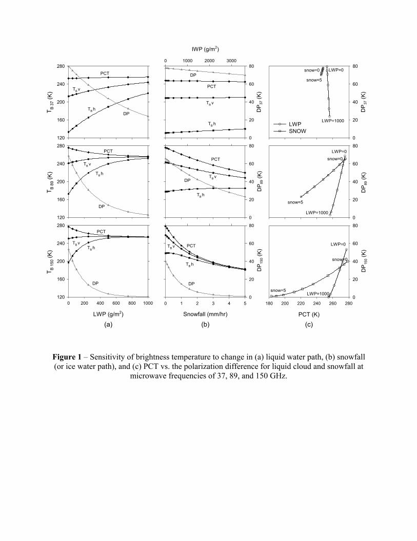
Figure 1 shows the brightness temperatures and their combinations at three
microwave frequencies (37, 89, and 150 GHz) in responding to the variation of liquid
water path and snowfall (or its corresponding ice water path). Two brightness
temperature combinations are considered: the polarization difference (DP=TB v - TB h) and
the polarization-corrected temperature as defined by Spencer et al. [1989], i.e.,
,)1( hTvTPCT BB αα −+= (1)
where TB v and TB h are, respectively, the vertically and horizontally polarized brightness
temperatures at each frequency. A value of α = 0.5 is used in (1), which is corresponding
to the value for January in the mid-latitudes suggested by Liu and Curry [1998]. Since
emission by liquid water and gases in the atmosphere reduces the polarization difference
of the radiation from the highly polarized ocean surface, the DP is representative of the
atmospheric emission. The PCT is used to reflect the brightness temperature depression
due to scattering by ice particles, and it is designed to have less influence by the
variations of water vapor and liquid water amount. In other words, while the decrease in
polarization difference largely responds to liquid water increase in the atmosphere, the
decrease of PCT represents the increase in the amount of scattering ice/snow particles
[Liu and Curry, 1998].
4

The left panel of Fig. 1 shows the model results when placing a liquid water cloud
between 1 and 1.5 km above the surface. The liquid water path (LWP) in the cloud varies
from 0 to 1000 g m-2. The snowfall-only modeling results are shown in the mid panel of
Fig. 1, in which snowfall rate is varied from 0 to 5 mm hr-1, and the snow layer is
assumed to be between the surface and 4 km. The corresponding ice water path (IWP) of
the snow layer is also shown in the figure. At 37 GHz, the brightness temperatures and
the polarization difference are closely related to the liquid water amount in the
atmosphere. A larger amount of liquid water responds to a higher brightness temperature
at both polarizations and a smaller DP. There is little response of microwave signals at 37
GHz to snowfall rate variation. At 89 and 150 GHz, as LWP increases, brightness
temperatures increase before saturating at about 1000 and 500 g m-2, respectively.
Brightness temperatures at these two channels show significant decreases as snowfall rate
(or IWP) increases, especially at 150 GHz. It is particularly noted that the variation of DP
is more sensitive to LWP changes, and the variation of PCT is more sensitive to snowfall
rate or IWP changes. To illustrate this observation, we re-plot the modeling results in DP-
PCT space (the right panel of Fig. 1), which show how the liquid water and snowfall
induce DP and PCT variations in the same chart. At 89 GHz, for example, as LWP
increases from 0 to 1000 g m-2, DP decreases by ~70 K while PCT decreases by ~20 K.
But as snowfall rate increases from 0 to 5 mm h-1, DP only reduces by ~ 40 K compared
to PCT reducing by ~ 60 K. The different responses of DP and PCT to liquid and ice
water are even clearer at 150 GHz. Therefore, more information of LWP contained in DP
is variations while PCT changes are more responsible to the variation in snowfall rate (or
5

IWP). Using these model simulation results as guidance, we examine satellite and
airborne microwave radiometer data in the following sections.
Data
Data from both satellite and airborne remote sensors are used to assess the
sensitivity of microwave radiation to snowfall over ocean by conducting two case studies
on January 29 and 30, 2003. This study period coincides with a field experiment carried
out near Japan for validating precipitation products from AMSR-E. The objectives of the
field experiment are examining the AMSR-E’s shallow rainfall and snowfall retrieval
capabilities and understanding the precipitation structures through new remote sensing
technology. Of the various datasets collected in the experiment, we analyze the data from
the following two remote sensors onboard a C-130 aircraft: the Millimeter-Wave Imaging
Radiometer (MIR) and the dual frequency Precipitation Radar (PR-2). The MIR is a total
power, cross-track scanning radiometer that measures radiation at seven frequencies of
89, 150, 183.3±1, 183.3±3, 183.3±7, 220, and 340 GHz [Racette et al., 1996]. The sensor
has a 3-db beam width of 3.5° at all frequencies. It can cover an angular swath up to ±50
degrees with respect to nadir. Every scan cycle is about three seconds [Wang, 2003]. The
PR-2 operates at 13.4 GHz (Ku-band) and 35.6 GHz (Ka-band), and uses a deployable
5.3-m electronically-scanned membrane antenna [Im, 2003].
Satellite data from two radiometers coincident with the field experiment are
analyzed. The AMSR-E is one of the six sensors aboard the Aqua satellite. This passive
microwave radiometer has vertically and horizontally polarized 6, 10, 19, 23, 37, and 89
GHz channels and vertically polarized 50 and 53 GHz channels. It conically scans the
6
Earth with an incident angle of ~55° to the normal of the Earth’s surface. The swath
width is about 1600 km. Spatial resolutions of the pixels are frequency dependent. At 37
and 89 GHz, which are frequencies examined in this study, they are 8×14 km2 and 3×6
km2, respectively. The Advanced Microwave Sounding Unit - B (AMSU-B) on board
the NOAA-16 has five channels at 89, 150, 183.3±1, 183.3±3, and 183.3±7 GHz.
Although the purpose of the AMSU-B is primarily for profiling atmospheric water vapor,
its window channels at 89 and 150 GHz also provide information of scattering by ice
particles [Zhao and Weng, 2002]. The AMSU-B crossly scans ± 47° from nadir, covering
approximately a 2000 km wide swath. The spatial resolution at nadir is ~16 km. Five of
the seven MIR channels operates at the same frequencies as the AMSU-B, so it offers a
unique comparison between satellite and aircraft measurements, between which there is a
huge difference in horizontal resolution.
Observed Snowfall Microwave Signatures
The two cases selected for this study are in the region of the Sea of Japan (Fig. 2) on
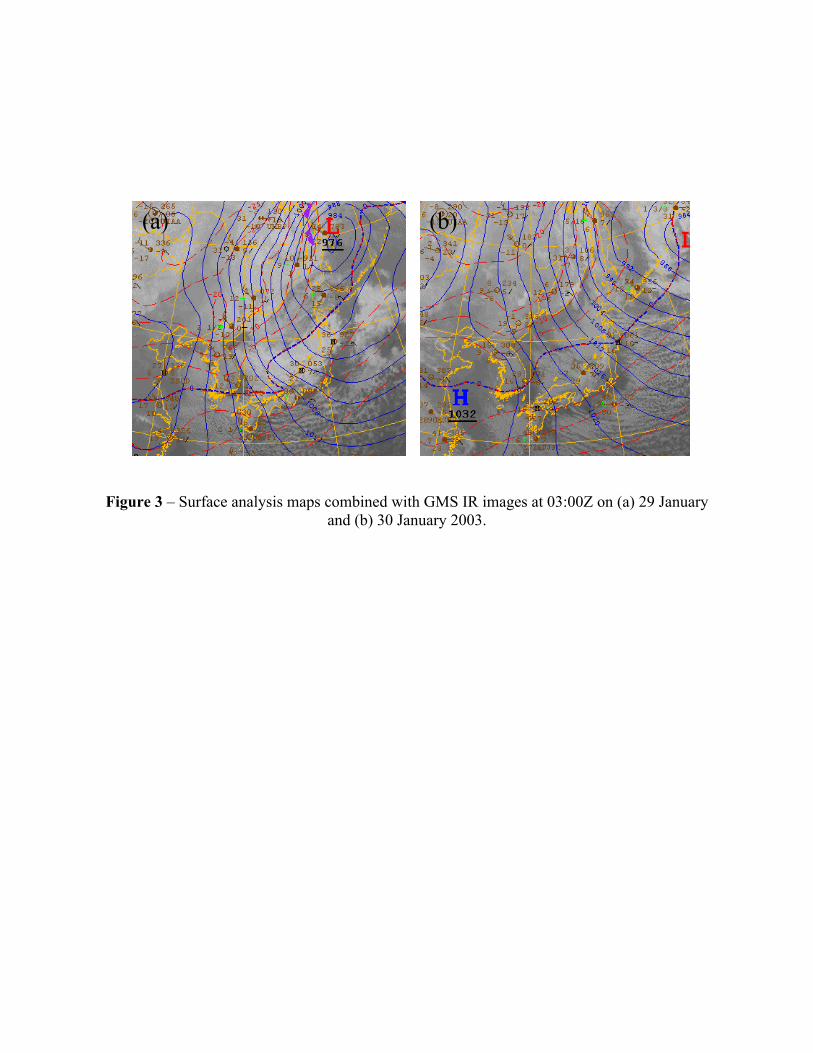
29 and 30 January 2003, when aircraft campaign was carried out. The synoptic conditions
for the two days can be seen from Fig. 3, in which the surface weather analysis is
overlaid with GMS (Geostationary Meteorological Satellite) infrared (IR) images. On 29
January 2003, a low-pressure system is centered near 50°N, 140°E and has center
pressure of 976 hPa (Fig. 3a). A strong northwesterly flow is dominant over the Sea of
Japan, and extensive snowfall areas were reported along the west coast of the main island
of Japan. An aircraft flight observing snowfall over ocean was conducted. Snowfall was
observed along the flight lines (A1 to B1 in Fig. 2, 36.5°N, 135.5°E and 38.5°N,
7

135.5°E) around 03:20Z. On 30 January 2003, the low seen in the previous day moved to
the east, resulting in a slightly reduced northwesterly flow across the Sea of Japan.
Snowfall was reported along the west coast of central Japan and was predicted over the
Sea of Japan. Widespread clouds were observed over the Sea of Japan, although from the
IR image they seemed to be not as deep as in the previous day. The aircraft flight was
conducted along several tracks including the line A2-B2 (36.33°N; 134.5°E to 38.67°N;
137.0°E in Fig. 2). In following sections, we will examine satellite and airborne
microwave radiometric signatures responded to the two cases.
Satellite observations
The Aqua satellite passed over the experiment area at 03:33Z on 29 January 2003.
Although there are frequencies from 6.6 to 89 GHz in AMSR-E, we only examine 37 and
89 GHz in the study because other channels are almost transparent to the snow clouds. At
37 and 89 GHz, the emissivity of the ocean surface is lower than unity. As a result, cloud
liquid water will increase the satellite received brightness temperatures. Meanwhile, both
cloud ice and snow in the atmosphere will decrease upwelling radiation due to ice
scattering.
Figure 4 shows the horizontal distributions of (a) and (e) vertically polarized
brightness temperatures, (b) and (f) horizontally polarized brightness temperatures, (c)
and (g) the polarization difference (DP=T hTv BB − ), and (d) and (h) the polarization-
corrected temperature (PCT with α = 0.5), at AMSR-E 89 GHz and 37 GHz. Fine
features can be identified from images of all the four variables. These features are
induced by clouds and their associated snowfall, since emission from ocean surface
8
should be more uniform horizontally. It is seen that there are several cloud cells between
37° and 38°N over ocean with relatively low brightness temperatures compared to their
surrounding background values. It is also noticed that the patterns of these cells are
different for different channels or brightness temperature combinations. The strongest
emission signal of polarization difference (<20 K) is found in the area around 37.2°N,
136.2°E. The centers of the lowest PCT are found slightly to the north of the center of the
lowest polarization difference.
To further elaborate, variations of the brightness temperatures along Line 1 and
Line 2 (refer Figs. 4d and 4h) are shown in Figs. 5 and 6. Figure 5 represents brightness
temperatures at 89 GHz and 37 GHz along Line 1 that overlaps the aircraft flight track on
29 January 2003. To compare two frequencies with different resolutions, data from both
frequencies are first interpolated to a 0.025o× 0.025o grid. Then, the brightness
temperature values along the line are obtained by averaging values of the nearest five
grids weighted by the inverse of the distance between the grid center and the line.
The results for 89 GHz are shown in Fig. 5a. Several small cells seen in Fig. 4
along Line 1 correspond to the decreases of 89 GHz brightness temperatures and PCT in
Fig. 5a. Note that a peak in horizontally polarized brightness temperatures is found at
37.2°N just before the decrease of PCT, and another peak at 37.4°N before the decrease
of PCT near 37.58°N. The lowest depression of PCT from the cloud-free value of ~260 K
is about 25 K near the cell centers. The largest decrease of the polarization difference is
~30 K near 37.2°N, and the location corresponds to the highest brightness temperature at
horizontal polarization. Figure 5b shows brightness temperatures at 37 GHz for the same
track (Line 1). The 37 GHz signals show less variations than those at 89 GHz, except for
9
a brightness temperature increase (the polarization difference decrease) near 37.2°N
corresponding to the first cell along Line 1 shown in Fig. 4d. Comparing 89 GHz and 37
GHz, a slight shift in the pattern of the polarization difference could be caused by the
different resolutions of two channels as well as the different response of brightness
temperatures to hydrometeors. The increase in 37 GHz brightness temperatures indicates
a significant amount of liquid water within the cell. However, either brightness
temperature or PCT at 37 GHz does not decrease corresponding to those decreases shown
in Fig. 5a for 89 GHz, indicating lack of response to scattering by cloud ice particles and
snowflakes. In other words, cloud ice particles and snowflakes produce measurable
scatter signatures at 89 GHz, but are largely not detectable at 37 GHz. The observational
results are consistent with the radiative transfer model results described earlier.
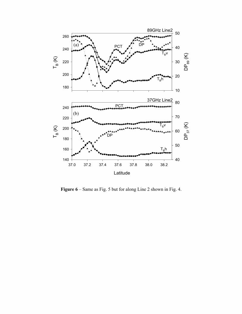
In Fig. 6 we show 89 GHz and 37 GHz data along another line that is shown as
Line 2 in Fig. 4. From Fig. 4, it was seen that this line crosses over a well-developed cell.
The lowest depression of PCT observed at 37.43°N is about 45 K at 89 GHz compared to
those at the cloud-free regions (~260 K). The depressions of brightness temperatures in
both polarizations are also much larger than those in Line 1. Similar to what occurred in
Line 1, the increase of horizontally polarized brightness temperatures (and the decrease
of the polarization difference) is shown before (south of) the PCT depressions. This
dislocation between the minima of PCT and polarization difference suggests that the
maxima of liquid water amount and snowfall rate occur at different locations within a cell.
At 37 GHz, the changes in vertically polarized brightness temperature and PCT are small
while horizontally polarized brightness temperature and polarization difference show
significant variations. The result further enforces our conclusion that while 37 GHz
10
channel is useful in determining liquid water path, it is incapable to detect snowfall. In an
attempt to see whether combining brightness temperatures at different frequencies offer
more information about the cloud and snowfall, the difference of brightness temperatures
between 89 GHz and 37 GHz along Line 1 are presented in Fig. 7. The vertically
polarized brightness temperature and PCT patterns reflect well-developed convective
cells shown in Fig. 4d. But this information is basically carried from the 89 GHz channel
because both TBv and PCT are largely flat at 37 GHz as shown in Fig. 5b.
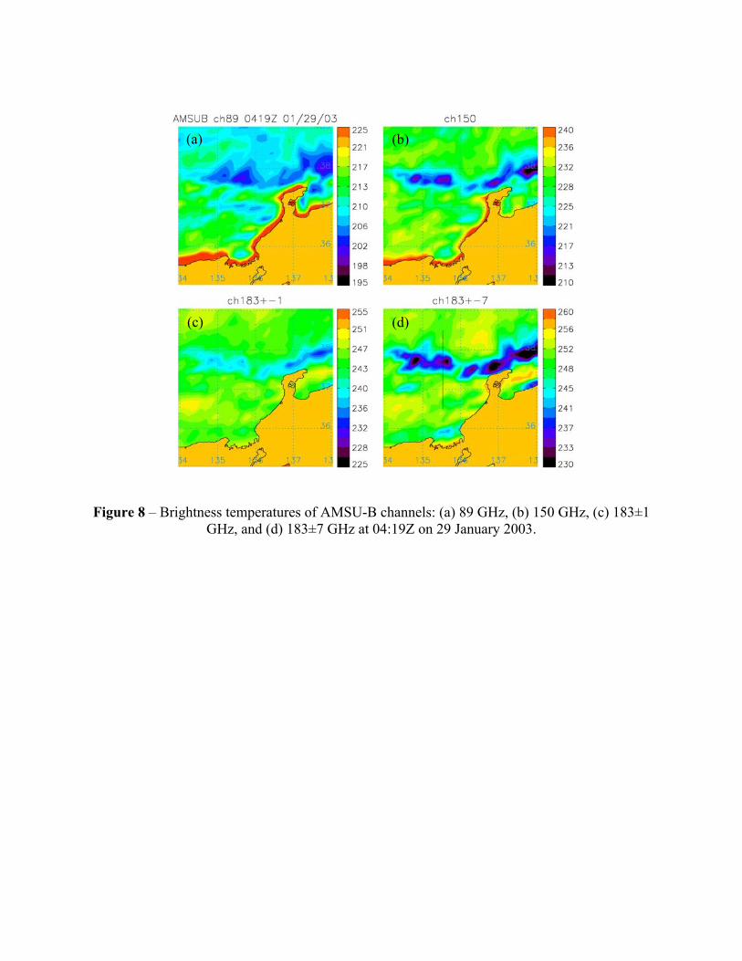
The NOAA-16 satellite passed the study area on 29 January 2003 at 04:19Z.
AMSU-B data on the NOAA-16 are also analyzed to explore the response to snowfall at
higher frequencies. Figure 8 shows brightness temperatures at four channels of 89, 150,
183±1, and 183±7 GHz (the 183±3 GHz image is not shown. Its image appears to be
between those of 183±1 and 183±7 GHz). Since AMSU-B channels contain only single
polarization, we are unable to derive PCT or polarization difference as was done for
AMSR-E channels. Additionally, because of the coarser spatial resolution, the images
appear lack of fine structures compared to those from AMSR-E in Fig. 4. Nevertheless,
low brightness temperature cells embedded on a long cloud streak are clearly shown
between 37°N and 38°N. The signals are particularly clear at 150 and 183±7 GHz. In
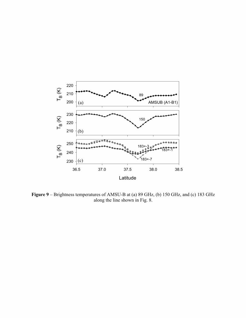
Fig. 9, brightness temperatures from the five AMSU-B channels are presented along the
line shown in Fig. 8, which corresponds to the aircraft flight track, Line 1 in Fig. 4. The
coarse spatial resolution reduced the sensitivity of radiation at 89 GHz, but significant
decreases in brightness temperatures at 150 GHz and 183±7 GHz are observed near the
snowfall cell at 37.7°N. The values of brightness temperature depression are about 15 K
at 150 GHz and 25 K at 183±7 GHz compared to nearby cloud-free regions. Comparing
11

to 89 GHz, the sensitivity to snowfall is much higher at 150 and 183±7 GHz. The
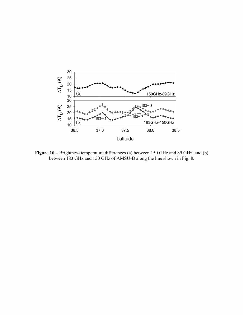
sensitivity at 183±1 and 183±3 GHz is not as large due to water vapor masking. Figure
10 shows the brightness temperature differences of two frequencies, 150 - 89 GHz and
183 - 150 GHz. While the difference of brightness temperatures between 183±7 and 150
GHz is relatively small, their differences between 183±1 and 150 GHz, and between
183±3 and 150 GHz are significant near the location of snowfall cells.
Case 2 is meant to show the response of microwave radiation to snowfall with
much less intensity (the weak snowfall was reported by airborne radar observations).
Figure 11 shows the brightness temperatures from AMSR-E at 04:14Z on 30 January
2003. The convective cells are aligned themselves along the streak clouds while they are
much smaller and weaker than those in the first case on 29 January 2003. In Fig. 11d, it is
seen that several small cells with low PCTs are orientated from northwest to southeast. At
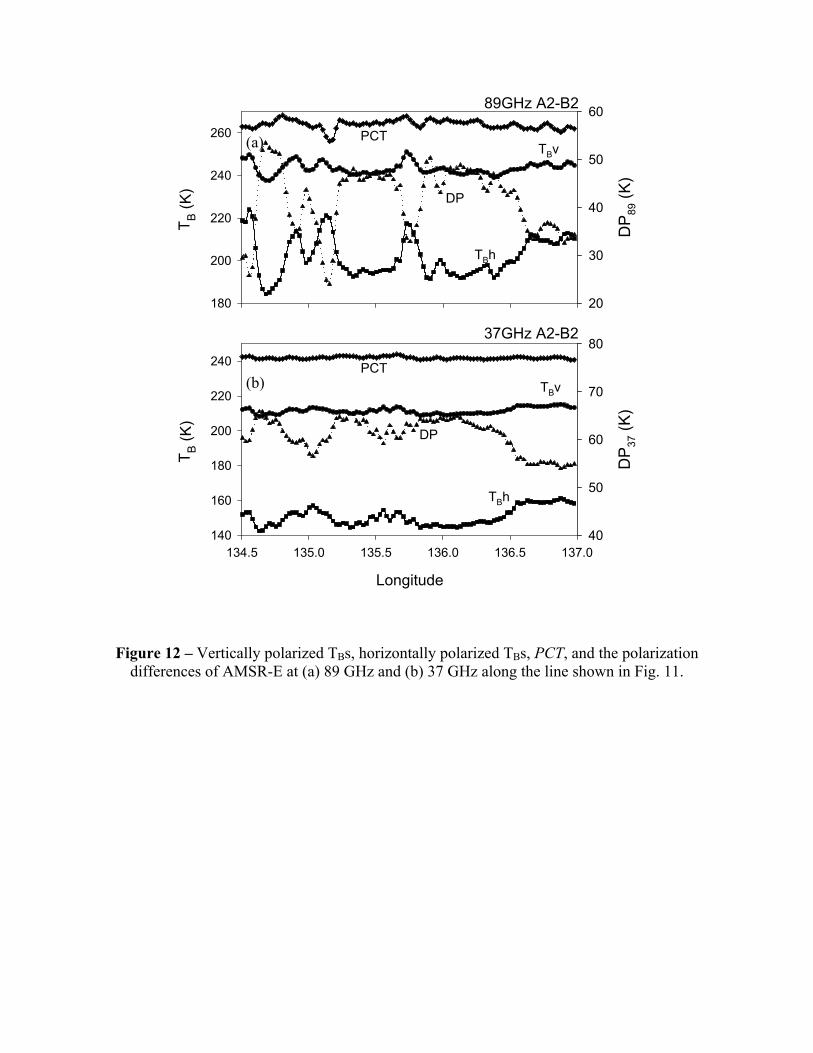
37 GHz, no significant signatures are identified along the track. The brightness
temperature values along the aircraft flight track (shown in Figs. 11d and 11h, or A2-B2
in Fig. 2) are shown in Fig. 12. The lowest PCT depression at 89 GHz in a cell center is
about 10 K near 135.2°E compared to surrounding cloud-free regions and the depression
is much smaller at 37 GHz. Unlike in the first case, in Fig. 12a, the maximum of the
horizontally polarized brightness temperature of about 220 K, the lowest PCT of about
257 K, and the lowest polarization difference of 23 K occur at almost the same position,
implying that the location of peak liquid water amount coincides with the location of the
strongest snowfall.
Airborne observations
12

The snow clouds on January 29 are observed by airborne radiometer MIR and
radar PR-2. One aircraft flight was carried out from 03:19Z to 03:33Z along the line of
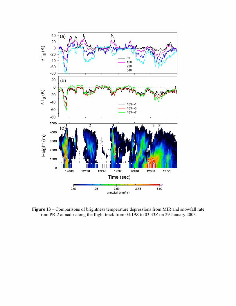
A1 to B1 as shown in Fig. 2 (corresponding to Line 1 in Fig. 4). In Fig. 13, we show the
aircraft nadir observations of the brightness temperature depressions compared to the
clear-sky values and the time-height cross section of snowfall rate converted from PR-2
13.4 GHz radar reflectivity. The clear-sky brightness temperatures are derived from
locations where no radar echo was observed; their values are 199.5, 218.7, 241.4, 250.6,
247.3, 243.8, and 255.7 K for 89, 150, 183±1, 183±3, 183±7, 220, and 340 GHz,
respectively. To obtain snowfall rate from radar reflectivity, we use a reflectivity-
snowfall rate (Ze-S) relation, although it may lead to significant uncertainties because of
the variety of shapes, densities, and terminal fall velocities of snowflakes [Matrosov,
1998]. In this study, we develop the following Ze-S relationship using the backscatter
cross sections calculated from discrete-dipole approximation modeling for snowflakes
[Liu, 2004] and particle size distribution based on Sekhon and Srivastava [1970]:
(2) ,151 083.1SZe =
where Ze is the equivalent radar reflectivity at 13.4 GHz in mm6 m-3, and S is the snowfall
rate in mm h-1.
In Fig. 13, five convective cells can be identified in the radar cross section as
indicated by numbers 1-5. The depression of MIR brightness temperatures responds to
these cells, although the sign and the amplitude of the variation are channel-dependent.
The depression of brightness temperature at 220 and 340 GHz is greater than the other
channels, and they reach about 80 K for the first cell. Among the three 183-GHz water
vapor channels, 183±7 GHz is the most sensitive to the snowfall cells. The second cell
13

seems to be weaker than the first one, and the brightness temperatures depression is also
smaller for all the channels. Note that at the starting point of the second cell a brightness
temperature peak appears at 89 GHz, suggesting that significant liquid water exists in
front of the center of the second snow cell. The third cell has rather different features,
especially at 89 and 150 GHz; brightness temperatures are much greater than those values
for the clear sky. It implies that the third cell contains a great amount of liquid water,
although strong radar echo is shown from 1 to 4 km. We divide the fifth cell into two
parts indicated as 5 and 5’ in Fig. 13c. The left region of the cell has the maximum
snowfall rate near the surface, but MIR brightness temperature depressions do not reach
their minimum until further into the middle of the cell as indicated by 5’ in the figure.
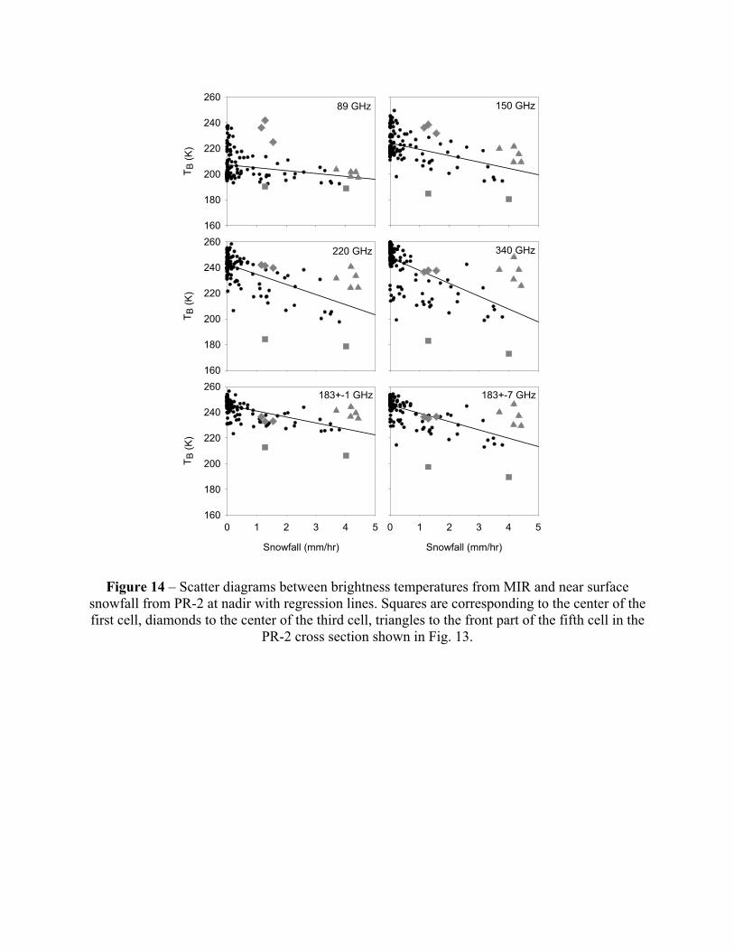
To quantitatively assess the relation between brightness temperature and near
surface snowfall rate, the brightness temperatures and radar reflectivity-derived snowfall
rate at 1 km (to avoid surface contamination) are averaged for every 10 seconds
(corresponding to ~1000 m in spatial scale) and plotted in Fig. 14. Brightness
temperatures in all the channels decrease in general as snowfall rates increase, although
there is a significant large range of scatter. A regression line for each channel is derived
using the 10-sec averaged data and plotted in the figure. The correlation coefficient is
-0.2, -0.46, -0.65, -0.67, -0.66, and -0.68 for data at 89, 150, 220, 340, 183±1, and 183±7
GHz, respectively. Based on these data, the sensitivity of brightness temperature to
snowfall rate can be estimated as -4, -10, -16, -22, -10, and -14.4 K (mm h-1)-1 for 89,
150, 220, 340, 183±1, and 183±7 GHz channels.
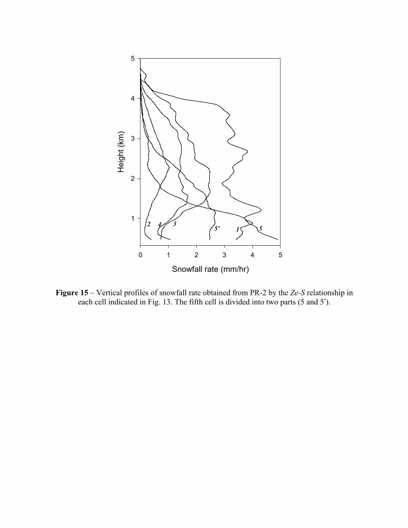
In Fig. 14, it is found that some points, as denoted by squares, diamonds, and
triangles, do not follow the general trend in the relationships. The two squares come from
14
the first cell; the radar-derived snowfall profile corresponding to the profile 1 in Fig. 15.
Strong radar returns are observed in a very deep layer, suggesting the center of a very
well developed convective cell. The diamonds correspond to the third cell, which has the
vertical radar profile 3 in Fig. 15. The strongest echo occurs in the middle of the layer (~
2 km), and the large increase in 89 GHz brightness temperatures implies a significant
amount of liquid water in the cell. These results suggest that cell 3 is in the early
developing stage, and the bulk of the condensed water is still in liquid form. The triangles
correspond to the first part of the fifth cell that has its bulk of radar returns near the
surface (profile 5 in Fig. 15). It is seen from Fig. 13c that the patterns of radar echoes for
cells 4 and 5 are vertically tilted, possibly caused by vertical wind shear. Although cell 5
as a whole reduced brightness temperatures significantly, the first part of the cell did not
cause sizable brightness temperature reduction because of only a shallow snowfall layer
existing near the surface. The above discussion illustrates how the horizontal and vertical
structures influence the observed brightness temperatures, and emphasizes the importance
of further observational studies to characterize the three-dimensional structure of snow
clouds.
Conclusions
In this study, we have investigated the scattering signals of snowfall over the Sea
of Japan at frequencies ranging from 37 to 340 GHz using satellite and aircraft
observations. The investigated snow clouds are associated with shallow convections
caused by cold air outbreaks. The cold air over the warm ocean surface produces strong
15

instability in the low atmosphere and often results in heavy snowfall. A significant
amount of liquid water is often observed in the convective cells as evidenced by the
increase in 89 GHz brightness temperatures.
At 37 GHz, the snowfall scattering signature seems to be insignificant, while
liquid water in some convective cells increases brightness temperature (as much as ~30 K
at 37 GHz horizontal polarization). At 89 GHz, the data shows both the brightness
temperature decreases due to ice scattering and brightness temperature increases due to
liquid water emission. Occasionally, these increases and decreases occur at different
locations of a convective cell. Observations using dual-polarization clearly have
advantage because we may use the polarization corrected temperature and the
polarization difference to separate, to a certain extent, the scattering and emission
signatures. Using AMSR-E data, the lowest PCT depression at 89 GHz is about 25 K for
one of the studied cases. However, the sensitivity to snowfall at 89 GHz is largely
reduced for AMSU-B, which has a much larger footprint and only a single polarization.
At higher frequencies, the snowfall signatures become evident even without the use of
PCT. At the spatial resolution of AMSU-B pixels (~16 km at nadir), we observed 15 ~ 20
K brightness temperature decreases at 150 and 183±7 GHz for the studied case. At finer
spatial resolution observed by airborne radiometers, the nadir view brightness
temperatures decrease as large as 40, 50, 60, and 80 K for 150, 183±7, 220, and 340 GHz
channels, respectively. Furthermore, the influence by liquid water to channels of 183±7
GHz or higher frequencies is small. At 150 GHz, besides the brightness temperature
decreases induced by ice scattering, the brightness temperature increases caused by liquid
water are also evident, similar to but not as much as those at 89 GHz. Therefore, having a
16

dual-polarization in future instruments for this frequency is desirable for a better
separation between liquid and ice water signatures.
In this study, we investigated the sensitivity of microwave channels to snowfall
over ocean, which may help the selection of channels in future instrument design.
Clearly, to have sufficiently strong scattering signature as well as to minimize the liquid
water influence, a high frequency (>150 GHz) and dual-polarization observations are
preferable. In order to develop a physically based algorithm to estimate snowfall, further
studies of more cases and analyses at various frequencies are recommended in
understanding the characteristics of the three-dimensional structures of snow clouds as
well as better simulating the scattering properties of snowflakes. This study would
provide a useful basis for future works on the retrieval of snowfall.
Acknowledgements. AMSR-E data are obtained from JAXA EORC. We thank Dr.
Ralph Ferraro of NOAA NESDIS for providing AMSU-B data. We also thank the team
of the NASA AMSR-E Wakasa field experiment for providing MIR and PR-2 data. This
research is supported by NASA grant NNG04GB04G and JAXA.
17

References
Bennartz R., Petty G. W. (2001) – The sensitivity of microwave remote sensing
observations of precipitation to ice particle size distribution. J. Appl. Meteor., 40: 345-
364.
Im E. (2003) – APR-2 Dual-Frequency Airborne Radar Observations, Wakasa Bay.
Boulder, CO: National Snow and Ice Data Center. Digital media. (Available at
http://nsidc.org/data/nsidc-0195.html)
Katsumata, M., Uyeda H., Iwanami K., Liu G. (2000) – The response of 36- and 89-
GHz microwave channels to convective snow clouds over ocean: observation and
modeling. J. Appl. Meteor., 39: 2322–2335.
Kummerow, C., Co-Authors (2000) – The Status of the Tropical Rainfall Measuring
Mission (TRMM) after Two Years in Orbit. J. Appl. Meteor., 39: 1965-1982.
Liu G. (1998) – A fast and accurate model for microwave radiance calculations. J.
Meteor. Soc. Japan, 76: 335-343.
Liu G. (2004) – Approximation of single-scattering properties of ice and snow particles
for high microwave frequencies. J. Atmos. Sci., 61: 2441-2456.
Liu G., Curry J. A. (1996) – Large-scale cloud features during January 1993 in the
North Atlantic Ocean as determined from SSM/I and SSM/T2. J. Geophys. Res., 101:
7019-7032.
Liu G., Curry J. A. (1997) – Precipitation characteristics in Greenland-Iceland-
Norwegian Seas determined by using satellite microwave data. J. Geophys. Res., 102:
13987-13997.
18

Liu G., Curry J. A. (1998) – An investigation of the relationship between emission and
scattering signals in SSM/I data. J. Atmos. Sci., 55: 1628-1643.
Liu G., Curry J. A. (2000) – Determination of ice water path and mass median particle
size using multichannel microwave measurements. J. Appl. Meteor., 39: 1318-1329.
Matrosov S. (1998) – A dual-wavelength radar method to measure snowfall rate. J. Appl.
Meteor., 37: 1510-1521.
Racette P., Adler R. F., Wang J. R., Gasiewski A. J., Jackson D. M., Zacharias D. S.
(1996) – An airborne Millimeter-wave Imaging Radiometer for cloud, precipitation, and
atmospheric water vapor studies. J. Atmos. Oceanic Technol., 13: 610-619.
Sekhon R. S., Srivastava R. C. (1970) – Snow size spectra and radar reflectivity. J. Atmos. Sci., 27: 299-307.
Schols J. L., Weinman J. A., Alexander G. D., Stewart R. E., Angus L. J., Lee C. L.
(1999) – Microwave properties of frozen precipitation around a North Atlantic Cyclone.
J. Appl. Meteor., 38: 29-43.
Spencer R. W., Goodman H. M., Hood R. E. (1989) – Precipitation retrieval over land
and ocean with SSM/I : Identification and characteristics of the scanning signals. J.
Atmos. Oceanic Technol., 6: 54-273.
Wang J. (2003) – Millimeter-wave Imaging Radiometer Brightness Temperatures,
Wakasa Bay, Japan. Boulder, CO: National Snow and Ice Data Center. Digital media.
(Available at http://nsidc.org/data/nsidc-0193.html)
Zhao L., Weng F. (2002) – Retrieval of ice cloud parameters using the Advanced
Microwave Sounding Unit. J. Appl. Meteor., 41: 384-395.
19
Caption of figures
Figure 1 – Sensitivity of brightness temperature to change in (a) liquid water path, (b)
snowfall (or ice water path), and (c) PCT vs. the polarization difference for liquid
cloud and snowfall at microwave frequencies of 37, 89, and 150 GHz.
Figure 2 – Map of the area where observations were performed and the aircraft flight
tracks.
Figure 3 – Surface analysis maps combined with GMS IR images at 03:00Z on (a) 29
January and (b) 30 January 2003.
Figure 4 – Brightness temperatures of AMSR-E at 89 GHz and 37 GHz: (a) and (e)
vertically polarized TBs, (b) and (f) horizontally polarized TBs, (c) and (g) the
polarization difference, DP, and (d) and (h) the polarization-corrected temperature,
PCT at 03:33Z on 29 January 2003.
Figure 5 – Vertically polarized TBs, horizontally polarized TBs, PCT, and the polarization
differences of AMSR-E at (a) 89 GHz and (b) 37 GHz along Line 1 shown in Fig.
4.
Figure 6 – Same as Fig. 5 but for along Line 2 shown in Fig. 4.
Figure 7 – Brightness temperature differences between 89 GHz and 37 GHz along Line1.
Figure 8 – Brightness temperatures of AMSU-B channels: (a) 89 GHz, (b) 150 GHz, (c)
183±1 GHz, and (d) 183±7 GHz at 04:19Z on 29 January 2003.
Figure 9 – Brightness temperatures of AMSU-B at (a) 89 GHz, (b) 150 GHz, and (c) 183
GHz along the line shown in Fig. 8.
Figure 10 – Brightness temperature differences (a) between 150 GHz and 89 GHz, and
(b) between 183 GHz and 150 GHz of AMSU-B along the line shown in Fig. 8.
Figure 11 – Brightness temperatures of AMSR-E at 89 GHz and 37 GHz: (a) and (e)
vertically polarized TBs, (b) and (f) horizontally polarized TBs, (c) and (g) the
polarization difference, DP, and (d) and (h) the polarization-corrected temperature,
PCT at 04:14Z on 30 January 2003.
20
21
Figure 12 – Vertically polarized TBs, horizontally polarized TBs, PCT, and the
polarization differences of AMSR-E at (a) 89 GHz and (b) 37 GHz along the line
shown in Fig. 11.
Figure 13 – Comparisons of brightness temperature depressions from MIR and snowfall
rate from PR-2 at nadir along the flight track from 03:19Z to 03:33Z on 29
January 2003.
Figure 14 – Scatter diagrams between brightness temperatures from MIR and near
surface snowfall from PR-2 at nadir with regression lines. Squares are
corresponding to the center of the first cell, diamonds to the center of the third cell,
triangles to the front part of the fifth cell in the PR-2 cross section shown in Fig.
13.
Figure 15 – Vertical profiles of snowfall rate obtained from PR-2 by the Ze-S relationship
in each cell indicated in Fig. 13. The fifth cell is divided into two parts (5 and 5’).
T B 37
(K)
120
160
200
240
280PCT
TB v
TB hDP
T B 89
(K)
120
160
200
240
280PCT
TB v
TB h
DP
LWP (g/m2)
(a)
0 200 400 600 800 1000
T B 15
0 (K
)
120
160
200
240
280PCT
TB vTB h
DP
DP 3
7 (K)
0
20
40
60
80
IWP (g/m2)
0 1000 2000 3000
PCT
TB v
TB h
DP
DP 8
9 (K)
0
20
40
60
80
PCT
TB v
TB h
DP
Snowfall (mm/hr)
(b)
0 1 2 3 4 5
DP 1
50 (K
)
0
20
40
60
80
PCTTB v
TB h
DP
DP 3
7 (K)
0
20
40
60
80
LWPSNOW
snow=5
LWP=0
DP 8
9 (K)
0
20
40
60
80
PCT (K)
(c)
180 200 220 240 260 280
DP 1
50 (K
)
0
20
40
60
80
snow=0
snow=5
snow=0
LWP=1000
LWP=1000
LWP=0
LWP=0
LWP=1000snow=5
snow=0
Figure 1 – Sensitivity of brightness temperature to change in (a) liquid water path, (b) snowfall (or ice water path), and (c) PCT vs. the polarization difference for liquid cloud and snowfall at
microwave frequencies of 37, 89, and 150 GHz.
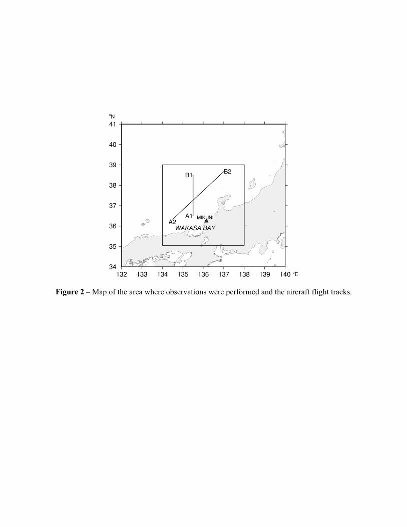
Figure 2 – Map of the area where observations were performed and the aircraft flight tracks.
(a) (b)
Figure 3 – Surface analysis maps combined with GMS IR images at 03:00Z on (a) 29 January
and (b) 30 January 2003.

(a) (b)
(d) (c)
(e) (f)
(h) (g)
Figure 4 – Brightness temperatures of AMSR-E at 89 GHz and 37 GHz: (a) and (e) vertically polarized TBs, (b) and (f) horizontally polarized TBs, (c) and (g) the polarization difference, DP,
and (d) and (h) the polarization-corrected temperature, PCT at 03:33Z on 29 January 2003.

89GHz Line1
T B (K
)
180
200
220
240
260
50
60
PCT TBv
37
T B (K
)
140
160
180
200
220
240
Figure 5 – Vertica
differences of A
(a)
DP
89 (K
)
20
30
40
TBhDP
37GHz Line1
70
80PCT
(b)
Latitude
.0 37.2 37.4 37.6 37.8 38.0 38.2
DP 37
(K)
40
50
60
TBv
TBh
DP
lly polarized TBs, horizontally polarized TBs, PCT, and the polarization MSR-E at (a) 89 GHz and (b) 37 GHz along Line 1 shown in Fig. 4.
89GHz Line2
T B (K
)
180
200
220
240
260
40
50
PCT DP
37
T B (K
)
140
160
180
200
220
240
Figur
(a)
DP
89 (K
)
10
20
30
TBv
TBh
37GHz Line2
Latitude
.0 37.2 37.4 37.6 37.8 38.0 38.2
DP 37
(K)
40
50
60
70
80PCT
TBv
TBh
DP
(b)
e 6 – Same as Fig. 5 but for along Line 2 shown in Fig. 4.

89GHz-37GHz Line1
Latitude
37.0 37.2 37.4 37.6 37.8 38.0 38.2
∆ TB (K
)
-10
0
10
20
30
40
50
60
PCT
TBv
TBh
Figure 7 – Brightness temperature differences between 89 GHz and 37 GHz along Line1.
(a) (b)
(c) (d)
Figure 8 – Brightness temperatures of AMSU-B channels: (a) 89 GHz, (b) 150 GHz, (c) 183±1
GHz, and (d) 183±7 GHz at 04:19Z on 29 January 2003.
AMSUB (A1-B1)T B (K
)
200
210
220
T B (K
)
210
220
230
36
T B (K
)
230
240
250
89
Figure 9 – Brightness
(a)
150
(b)
183+-7
183+-3183+-1
(c)
Latitude
.5 37.0 37.5 38.0 38.5
temperatures of AMSU-B at (a) 89 GHz, (b) 150 GHz, and (c) 183 GHz along the line shown in Fig. 8.
150GHz-89GHz∆ TB
(K)
1015202530
36
∆ TB
(K)
1015202530
Figure 10 – Brightnbetween 183
(a)
183GHz-150GHz183+-7
183+-3
183+-1
(b)Latitude
.5 37.0 37.5 38.0 38.5
ess temperature differences (a) between 150 GHz and 89 GHz, and (b) GHz and 150 GHz of AMSU-B along the line shown in Fig. 8.

(b) (a)
(d) (c)
(f) (e)
(h) (g)
Figure 11 – Brightness temperatures of AMSR-E at 89 GHz and 37 GHz: (a) and (e) vertically polarized TBs, (b) and (f) horizontally polarized TBs, (c) and (g) the polarization difference, DP,
and (d) and (h) the polarization-corrected temperature, PCT at 04:14Z on 30 January 2003.
89GHz A2-B2
T B (K
)
180
200
220
240
260
DP
89 (K
)
20
30
40
50
60
PCTTBv
TBh
DP
(a)
37GHz A2-B2
Longitude
134.5 135.0 135.5 136.0 136.5 137.0
T B (K
)
140
160
180
200
220
240
DP 37
(K)
40
50
60
70
80
PCTTBv
TBh
DP
(b)
Figure 12 – Vertically polarized TBs, horizontally polarized TBs, PCT, and the polarization differences of AMSR-E at (a) 89 GHz and (b) 37 GHz along the line shown in Fig. 11.
∆ TB
(K)
-80-60-40-20
02040
89150220340
∆ TB
(K)
-80
-60
-40
-20
0
20
183+-1183+-3183+-7
(a)
(b)
(c
Figure 13 – Comfrom PR-2 at
) 1 2 3 4 5 5’
parisons of brightness temperature depressions from MIR and snowfall rate nadir along the flight track from 03:19Z to 03:33Z on 29 January 2003.
89 GHz
T B (K
)
160
180
200
220
240
260150 GHz
183+-1 GHz
Snowfall (mm/hr)
0 1 2 3 4 5
T B (K
)
160
180
200
220
240
260183+-7 GHz
Snowfall (mm/hr)
0 1 2 3 4 5
340 GHz220 GHz
T B (K
)
160
180
200
220
240
260
Figure 14 – Scatter diagrams between brightness temperatures from MIR and near surface snowfall from PR-2 at nadir with regression lines. Squares are corresponding to the center of the first cell, diamonds to the center of the third cell, triangles to the front part of the fifth cell in the
PR-2 cross section shown in Fig. 13.
Snowfall rate (mm/hr)
0 1 2 3 4 5
Hei
ght (
km)
1
2
3
4
5
12 3
55'4
Figure 15 – Vertical profiles of snowfall rate obtained from PR-2 by the Ze-S relationship in each cell indicated in Fig. 13. The fifth cell is divided into two parts (5 and 5’).


