
Solving Polynomial Systems in Noether Positionwith Puiseux Series
Danko Adrovic
(joint work with Jan Verschelde)
University of Illinois at Chicago
www.math.uic.edu/~adrovic
2013 SIAM Conference on Applied Algebraic Geometry- Algorithms in Numerical Algebraic Geometry -
Colorado State UniversityFort Collins, Colorado
Danko Adrovic (UIC) Solving Polynomial Systems August 2nd , 2013 1 / 24
Talk Outline
a new polyhedral method
development of positive dimensional solution setsfor square systems and systems with more equations than unknowns
i.e. systems where positive dimensional solution sets are not expected
in applications
cyclic n-roots problem
main result
tropical version of Backelin’s Lemma
Danko Adrovic (UIC) Solving Polynomial Systems August 2nd , 2013 2 / 24
Polyhedral Method Description
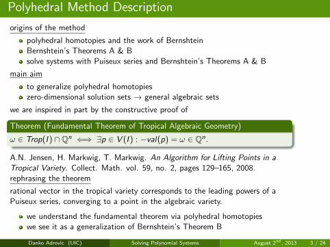
origins of the method
polyhedral homotopies and the work of BernshteinBernshtein’s Theorems A & Bsolve systems with Puiseux series and Bernshtein’s Theorems A & B
main aim
to generalize polyhedral homotopieszero-dimensional solution sets → general algebraic sets
we are inspired in part by the constructive proof of
Theorem (Fundamental Theorem of Tropical Algebraic Geometry)
ω ∈ Trop(I ) ∩Qn ⇐⇒ ∃p ∈ V (I ) : −val(p) = ω ∈ Qn.
A.N. Jensen, H. Markwig, T. Markwig. An Algorithm for Lifting Points in aTropical Variety. Collect. Math. vol. 59, no. 2, pages 129–165, 2008.rephrasing the theorem
rational vector in the tropical variety corresponds to the leading powers of aPuiseux series, converging to a point in the algebraic variety.
we understand the fundamental theorem via polyhedral homotopieswe see it as a generalization of Bernshtein’s Theorem B
Danko Adrovic (UIC) Solving Polynomial Systems August 2nd , 2013 3 / 24

General Definitions
Definition (Polynomial System)
F (x) =
f0(x) = 0f1(x) = 0...fn−1(x) = 0
Definition (Laurent Polynomial)
f (x) =∑a∈A
caxa, ca ∈ C \ {0}, xa = x±a0
0 x±a11 · · · x±an−1
n−1
Definition (Support Set)
The set of exponents Ai is called the support set of fi .
Definition (Newton Polytope)
Let Ai be the support set of the polynomial fi ∈ F(x) = 0. Then,the Newton polytope of fi is the convex hull of Ai , denoted Pi .
Danko Adrovic (UIC) Solving Polynomial Systems August 2nd , 2013 4 / 24

General Definitions
Definition (Initial Form)
Let f (x) =∑a∈A
caxa be a Laurent polynomial, v ∈ Zn a non-zero vector and let 〈·, ·〉
denote the usual inner product. Then, the initial form with respect to v is given by
inv(f (x)) =∑
a∈A, m=〈a,v〉
caxa
m = min {〈a, v〉 | a ∈ A}
where the minimal value m has been achieved at least twice.
Definition (Initial Form System)
For a system of polynomials F(x) = 0, the initial form system is defined byinv(F(x)) = (inv(f0), inv(f1), . . . , inv(fn−1)) = 0.
Definition (Pretropism)
A pretropism v ∈ Zn is a vector, common to all Newton polytopes of thepolynomial system. A pretropism leads to an initial form system.
Definition (Tropism)
A tropism is a pretropism, which is the leading exponent vector in a Puiseux seriesexpansion of a curve, expanded about t ≈ 0.
Danko Adrovic (UIC) Solving Polynomial Systems August 2nd , 2013 5 / 24

The Cayley Embedding & Polytope For Square Systems
We obtain pretropisms for polynomial systems using the Cayley polytope.
Cayley Embedding
CE = (A0 × {0}) ∪ (A1 × {e1}) ∪ · · · ∪ (An−1 × {en−1})
where ek is the k-th (n − 1)-dimensional standard unit vector.
Cayley Polytope
C∆ = ConvexHull(CE )
Remark
We use the Cayley polytope as a way to combine all individual Newtonpolytopes into one Cayley polytope and obtain their common facetnormals.
We use cddlib of K. Fukuda to find facet normals of the Cayley polytope.Alternative: gfan, developed by A.N. Jensen, finds cones of pretropisms.
Danko Adrovic (UIC) Solving Polynomial Systems August 2nd , 2013 6 / 24

Tropisms and d-Dimensional Surfaces
For d-dimensional solution sets we have cones of tropisms.
Definition (Cone of Tropisms)
A cone of tropisms is a polyhedral cone, spanned by tropisms.
v0, v1, . . . , vd−1 span a d-dimensional cone of tropismsdimension of the cone is the dimension of the solution set
Let v0 = (v(0,1), v(0,2), . . . , v(0,n−1)), v1 = (v(1,0), v(1,1), . . . , v(1,n−1)), . . . ,vd−1 = (v(d−1,0), v(d−1,1), . . . , v(d−1,n−1)) be d tropisms. Let r0, r1, . . . , rn−1 bethe solutions of the initial form system inv0(inv1(· · · invd−1
(F ) · · · ))(x) = 0.
d tropisms generate a Puiseux series expansion of a d-dimensional surface
x0 = tv(0,0)
0 tv(1,0)
1 · · · tv(d−1,0)
d−1 (r0 + c(0,0)tw(0,0)
0 + c(1,0)tw(1,0)
1 + . . . )
x1 = tv(0,1)
0 tv(1,1)
1 · · · tv(d−1,1)
d−1 (r1 + c(0,1)tw(0,1)
0 + c(1,1)tw(1,1)
1 + . . . )
x2 = tv(0,2)
0 tv(1,2)
1 · · · tv(d−1,2)
d−1 (r2 + c(0,2)tw(0,2)
0 + c(1,2)tw(1,2)
1 + . . . )
...
xn−1 = tv(0,n−1)
0 tv(1,n−1)
1 · · · tv(d−1,n−1)
d−1 (rn−1 + c(0,n−1)tw(0,n−1)
0 + c(1,n−1)tw(1,n−1)
1 + . . . )
Danko Adrovic (UIC) Solving Polynomial Systems August 2nd , 2013 7 / 24

Unimodular Coordinate Transformation
Definition (Unimodular Coordinate Transformation)
Let M ∈ Zn×n be a matrix with det(M) = ±1. Then, the unimodular coordinatetransformation is a power transformation of the form x = zM .
matrix M
contains the d dimensional cone tropisms in their first d rowsused to transform
initial form systems i.e. inv(F )(x = zM)) → isolated solutions at infinitypolynomial systems → second term in the Puiseux series
x = zM puts solution sets in a specific format
Our method to obtain matrix M uses the computation of:
Smith Normal Form (for series with integer exponents)Hermite Normal Form (for series with fractional exponents)
Related result: E. Hubert and G. Labahn. Rational invariants of scalingsfrom Hermite normal forms. In Proceedings of ISSAC 2012, pages 219226.ACM, 2012.
Danko Adrovic (UIC) Solving Polynomial Systems August 2nd , 2013 8 / 24

General Algebraic Sets
Assumptions on the solution sets we can find
Proposition If F (x) = 0 is in Noether position and defines a d-dimensionalsolution set in Cn, intersecting the first d coordinate planes in regular isolatedpoints, then there are d linearly independent tropisms v0, v1, . . . vd−1 ∈ Qn so thatthe initial form system inv0(inv1(· · · invd−1
(F ) · · · ))(x = zM) = 0 has a solutionc ∈ (C \ {0})n−d . This solution and the tropisms are the leading coefficients andpowers of a generalized Puiseux series expansion for the algebraic set:
x0 = tv0,0
0
x1 = tv0,1
0 tv1,1
1...
xd−1 = tv0,d−1
0 tv1,d−1
1 · · · tvd−1,d−1
d−1
xd = c0tv0,d
0 tv1,d
1 · · · tvd−1,d
d−1 + · · ·
xd+1 = c1tv0,d+1
0 tv1,d+1
1 · · · tvd−1,d+1
d−1 + · · ·...
xn = cn−d−1tv0,n−1
0 tv1,n−1
1 · · · tvd−1,n−1
d−1 + · · ·
Danko Adrovic (UIC) Solving Polynomial Systems August 2nd , 2013 9 / 24

Cyclic n-roots Problem
Cn(x) =
x0 + x1 + · · ·+ xn−1 = 0
x0x1 + x1x2 + · · ·+ xn−2xn−1 + xn−1x0 = 0
i = 3, 4, . . . , n − 1 :n−1∑j=0
j+i−1∏k=j
xk mod n = 0
x0x1x2 · · · xn−1 − 1 = 0.
benchmark problem in the field of computer algebra (pop. by J. Davenport)extremely hard to solve for n ≥ 8square systems
we expect isolated solutionswe find positive dimensional solution sets
Lemma (Backelin)
If m2 divides n, then the dimension of the cyclic n-roots polynomial system is atleast m − 1.
J. Backelin: Square multiples n give infinitely many cyclic n-roots.Reports, Matematiska Institutionen, Stockholms Universitet, 1989.J. Davenport. Looking at a set of equations.Technical Report 87-06, Bath Computer Science, 1987.
Danko Adrovic (UIC) Solving Polynomial Systems August 2nd , 2013 10 / 24
Cyclic 8-Roots System
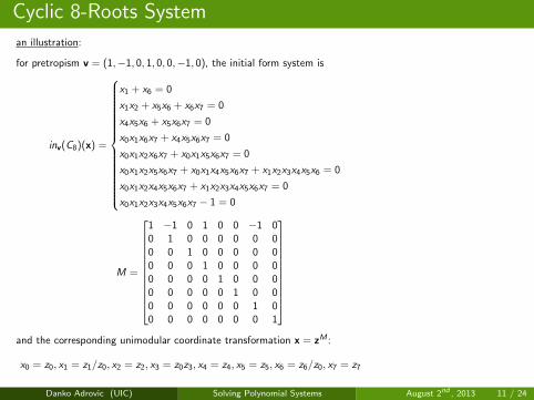
an illustration:
for pretropism v = (1,−1, 0, 1, 0, 0,−1, 0), the initial form system is
inv(C8)(x) =
x1 + x6 = 0
x1x2 + x5x6 + x6x7 = 0
x4x5x6 + x5x6x7 = 0
x0x1x6x7 + x4x5x6x7 = 0
x0x1x2x6x7 + x0x1x5x6x7 = 0
x0x1x2x5x6x7 + x0x1x4x5x6x7 + x1x2x3x4x5x6 = 0
x0x1x2x4x5x6x7 + x1x2x3x4x5x6x7 = 0
x0x1x2x3x4x5x6x7 − 1 = 0
M =
1 −1 0 1 0 0 −1 00 1 0 0 0 0 0 00 0 1 0 0 0 0 00 0 0 1 0 0 0 00 0 0 0 1 0 0 00 0 0 0 0 1 0 00 0 0 0 0 0 1 00 0 0 0 0 0 0 1
and the corresponding unimodular coordinate transformation x = zM :
x0 = z0, x1 = z1/z0, x2 = z2, x3 = z0z3, x4 = z4, x5 = z5, x6 = z6/z0, x7 = z7
Danko Adrovic (UIC) Solving Polynomial Systems August 2nd , 2013 11 / 24
Cyclic 8-Roots System
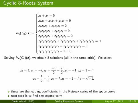
inv(C8)(z) =
z1 + z6 = 0
z1z2 + z5z6 + z6z7 = 0
z4z5z6 + z5z6z7 = 0
z4z5z6z7 + z1z6z7 = 0
z1z2z6z7 + z1z5z6z7 = 0
z1z2z3z4z5z6 + z1z2z5z6z7 + z1z4z5z6z7 = 0
z1z2z3z4z5z6z7 + z1z2z4z5z6z7 = 0
z1z2z3z4z5z6z7 − 1 = 0
Solving inv(C8)(z), we obtain 8 solutions (all in the same orbit). We select
z0 = t, z1 = −i , z2 =−1
2− i
2, z3 = −1, z4 = 1 + i ,
z5 =1
2+
i
2, z6 = i , z7 = −1− i , i =
√−1.
these are the leading coefficients in the Puiseux series of the space curvenext step is to find the second term
Danko Adrovic (UIC) Solving Polynomial Systems August 2nd , 2013 12 / 24

Cyclic 8-Roots System
Proposition If the initial root does not satisfy the entire transformedpolynomial system, then there must be at least one nonzero constantexponent ai , forming monomial ci t
ai .
illustration
r1 = −i , r2 =−1
2− i
2, r3 = −1, r4 = 1 + i , r5 =
1
2+
i
2, r6 = i , r7 = −1− i
Substituting the form zi = ri + ki tw , i = 1 . . . n − 1, into the transformed
system C8(z), yields
tw (...) + ...
t2(...) + ...
tw (...) + ...
4t + tw (...) + ...
tw (...) + ...
t2(...) + ...
tw (...) + ...
tw (...) + ...
in this case ci tai = 4t1
Danko Adrovic (UIC) Solving Polynomial Systems August 2nd , 2013 13 / 24

Cyclic 8-Roots System
Taking solution atinfinity, we build aseries of the form:
z0 = t
z1 = −I + k1t
z2 =−1
2− I
2+ k2t
z3 = −1 + k3t
z4 = 1 + I + k4t
z5 =1
2+
I
2+ k5t
z6 = I + k6t
z7 = (−1− I ) + k7t
Plugging series forminto transformedsystem, collecting allcoefficients of t1 andsolving, yields
k1 = −1− I
k2 =1
2k3 = 0
k4 = −1
k5 =−1
2k6 = 1 + I
k7 = 1
The second term inthe series, still in thetransformedcoordinates:
z0 = t
z1 = −I + (−1− I )t
z2 =−1
2− I
2+
1
2t
z3 = −1
z4 = 1 + I − t
z5 =1
2+
I
2− 1
2t
z6 = I + (1 + I )t
z7 = (−1− I ) + t
Danko Adrovic (UIC) Solving Polynomial Systems August 2nd , 2013 14 / 24

Cyclic 4,8,12-roots problem
Often, first term in the Puiseux satisfies the entire system:
cyclic 4-roots:tropism: (1,-1,1,-1)
x0 = t, x1 = t−1, x2 = −t, x3 = −t−1
cyclic 8-roots:tropism: (1,-1,1,-1,1,-1,1,-1)
x0 = t, x1 = t−1, x2 = it, x3 = it−1, x4 = −t, x5 = −t−1,x6 = −it, x7 = −it−1
cyclic 12-roots:tropism: (1,-1,1,-1, 1,-1,1,-1,1,-1,1,-1)
x0 = t, x1 = t−1, x2 = ( 1+√
3i2 )t, x3 = ( 1+
√3i
2 )t−1,
x4 = (−1+√
3i2 )t, x5 = (−1+
√3i
2 )t−1, x6 = −t, x7 = −t−1,
x8 = (−1−√
3i2 )t, x9 = (−1−
√3i
2 )t−1, x10 = ( 1−√
3i2 )t, x11 = ( 1−
√3i
2 )t−1
Observing structure among
tropismcoefficients
numerical solver PHCpack was usedwe recognize the coefficients as n
2 -roots of unity
Danko Adrovic (UIC) Solving Polynomial Systems August 2nd , 2013 15 / 24
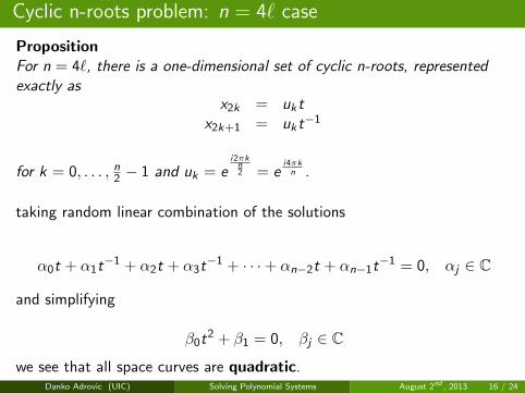
Cyclic n-roots problem: n = 4` case
PropositionFor n = 4`, there is a one-dimensional set of cyclic n-roots, representedexactly as
x2k = uktx2k+1 = ukt−1
for k = 0, . . . , n2 − 1 and uk = ei2πkn2 = e
i4πkn .
taking random linear combination of the solutions
α0t + α1t−1 + α2t + α3t−1 + · · ·+ αn−2t + αn−1t−1 = 0, αj ∈ C
and simplifying
β0t2 + β1 = 0, βj ∈ C
we see that all space curves are quadratic.Danko Adrovic (UIC) Solving Polynomial Systems August 2nd , 2013 16 / 24
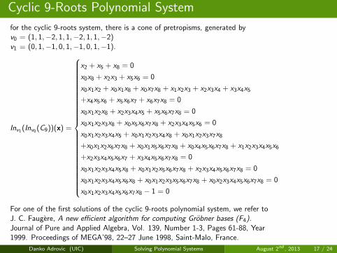
Cyclic 9-Roots Polynomial System
for the cyclic 9-roots system, there is a cone of pretropisms, generated byv0 = (1, 1,−2, 1, 1,−2, 1, 1,−2)v1 = (0, 1,−1, 0, 1,−1, 0, 1,−1).
Inv1(Inv0(C9))(x) =
x2 + x5 + x8 = 0
x0x8 + x2x3 + x5x6 = 0
x0x1x2 + x0x1x8 + x0x7x8 + x1x2x3 + x2x3x4 + x3x4x5
+x4x5x6 + x5x6x7 + x6x7x8 = 0
x0x1x2x8 + x2x3x4x5 + x5x6x7x8 = 0
x0x1x2x3x8 + x0x5x6x7x8 + x2x3x4x5x6 = 0
x0x1x2x3x4x5 + x0x1x2x3x4x8 + x0x1x2x3x7x8
+x0x1x2x6x7x8 + x0x1x5x6x7x8 + x0x4x5x6x7x8 + x1x2x3x4x5x6
+x2x3x4x5x6x7 + x3x4x5x6x7x8 = 0
x0x1x2x3x4x5x8 + x0x1x2x5x6x7x8 + x2x3x4x5x6x7x8 = 0
x0x1x2x3x4x5x6x8 + x0x1x2x3x5x6x7x8 + x0x2x3x4x5x6x7x8 = 0
x0x1x2x3x4x5x6x7x8 − 1 = 0
For one of the first solutions of the cyclic 9-roots polynomial system, we refer toJ. C. Faugere, A new efficient algorithm for computing Grobner bases (F4).Journal of Pure and Applied Algebra, Vol. 139, Number 1-3, Pages 61-88, Year1999. Proceedings of MEGA’98, 22–27 June 1998, Saint-Malo, France.
Danko Adrovic (UIC) Solving Polynomial Systems August 2nd , 2013 17 / 24

Cyclic 9-Roots Polynomial System Cont.
v0 =( 1, 1, -2, 1, 1, -2, 1, 1, -2 )v1 =( 0, 1, -1, 0, 1, -1, 0, 1, -1 )The unimodular coordinate transformation x = zM acts on the exponents.The new coordinates are given by
M =
1 1 −2 1 1 −2 1 1 −20 1 −1 0 1 −1 0 1 −10 0 1 0 0 0 0 0 00 0 0 1 0 0 0 0 00 0 0 0 1 0 0 0 00 0 0 0 0 1 0 0 00 0 0 0 0 0 1 0 00 0 0 0 0 0 0 1 00 0 0 0 0 0 0 0 1
x0 = z0
x1 = z0z1
x2 = z−20 z−1
1 z2
x3 = z0z3
x4 = z0z1z4
x5 = z−20 z−1
1 z5
x6 = z0z6
x7 = z0z1z7
x8 = z−20 z−1
1 z8
We use the coordinate change to transform the initial form system and theoriginal cyclic 9-roots system.
Danko Adrovic (UIC) Solving Polynomial Systems August 2nd , 2013 18 / 24

Cyclic 9-Roots Polynomial System Cont.
The transformed initial form system inv1(inv0(C9))(z) is given by
z2 + z5 + z8 = 0
z2z3 + z5z6 + z8 = 0
z2z3z4 + z3z4z5 + z4z5z6 + z5z6z7 + z6z7z8 + z2z3 + z7z8 + z2 + z8 = 0
z2z3z4z5 + z5z6z7z8 + z2z8 = 0
z2z3z4z5z6 + z5z6z7z8 + z2z3z8 = 0
z2z3z4z5z6z7 + z3z4z5z6z7z8 + z2z3z4z5z6 + z4z5z6z7z8 + z2z3z4z5 + z2z3z4z8
+z2z3z7z8 + z2z6z7z8 + z5z6z7z8 = 0
z3z4z6z7 + z3z4 + z6z7 = 0
z4z7 + z4 + z7 = 0
z2z3z4z5z6z7z8 − 1 = 0
Its solution isz2 = −1
2 −√
3i2 , z3 = −1
2 +√
3i2 , z4 = −1
2 +√
3i2 , z5 = 1, z6 = −1
2 −√
3i2 ,
z7 = −12 −
√3i
2 , z8 = −12 +
√3i
2 , where i =√−1.
While we used a numerical solver PHCpack, we recognized the solution asthe 3rd roots of unity.
Danko Adrovic (UIC) Solving Polynomial Systems August 2nd , 2013 19 / 24
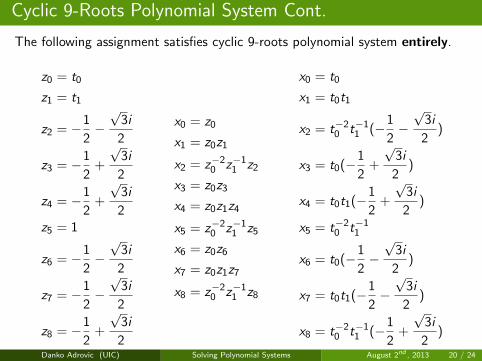
Cyclic 9-Roots Polynomial System Cont.
The following assignment satisfies cyclic 9-roots polynomial system entirely.
z0 = t0
z1 = t1
z2 = −1
2−√
3i
2
z3 = −1
2+
√3i
2
z4 = −1
2+
√3i
2z5 = 1
z6 = −1
2−√
3i
2
z7 = −1
2−√
3i
2
z8 = −1
2+
√3i
2
x0 = z0
x1 = z0z1
x2 = z−20 z−1
1 z2
x3 = z0z3
x4 = z0z1z4
x5 = z−20 z−1
1 z5
x6 = z0z6
x7 = z0z1z7
x8 = z−20 z−1
1 z8
x0 = t0
x1 = t0t1
x2 = t−20 t−1
1 (−1
2−√
3i
2)
x3 = t0(−1
2+
√3i
2)
x4 = t0t1(−1
2+
√3i
2)
x5 = t−20 t−1
1
x6 = t0(−1
2−√
3i
2)
x7 = t0t1(−1
2−√
3i
2)
x8 = t−20 t−1
1 (−1
2+
√3i
2)
Danko Adrovic (UIC) Solving Polynomial Systems August 2nd , 2013 20 / 24

Cyclic 9-Roots Polynomial System Cont.
Letting u = e2πi
3 and y0 = t0, y1 = t0t1, y2 = t−20 t−1
1 u2
we can rewrite the exact solution as
x0 = t0 x3 = t0u x6 = t0u2
x1 = t0t1 x4 = t0t2u x7 = t0t2u2
x2 = t−20 t−1
1 u2 x5 = t−20 t−1
1 x8 = t−20 t−1
1 u
x0 = y0 x3 = y0u x6 = y0u2
x1 = y1 x4 = y1u x7 = y1u2
x2 = y2 x5 = y2u x8 = y2u2
and put it in the same format as in the proof of Backelin’s Lemma, given inJ. C. Faugere, Finding all the solutions of Cyclic 9 using Grobner basistechniques. In Computer Mathematics: Proceedings of the Fifth AsianSymposium (ASCM), pages 1-12. World Scientific, 2001.
degree of the solution component
α1t0 + α2t0t1 + α3t−20 t−1
1 = 0
α4t0 + α5t0t1 + α6t−20 t−1
1 = 0αi ∈ C
Simplifying, the system becomes
t−20 t−1
1 − β1 = 0
t1 − β2 = 0
As the simplified system has 3 solutions, the cyclic 9 solution componentis a cubic surface. With the cyclic permutation, we obtain an orbit of 6cubic surfaces, which satisfy the cyclic 9-roots system.
Danko Adrovic (UIC) Solving Polynomial Systems August 2nd , 2013 21 / 24

Cyclic 16-Roots Polynomial System
Extending the pattern we observed among tropisms of the cyclic 9-roots,v0 = (1, 1,−2, 1, 1,−2, 1, 1,−2)v1 = (0, 1,−1, 0, 1,−1, 0, 1,−1)we can get the correct cone of tropisms for the cyclic 16-roots.v0 = (1, 1, 1,−3, 1, 1, 1,−3, 1, 1, 1,−3, 1, 1, 1,−3)v1 = (0, 1, 1,−2, 0, 1, 1,−2, 0, 1, 1,−2, 0, 1, 1,−2)v2 = (0, 0, 1,−1, 0, 0, 1,−1, 0, 0, 1,−1, 0, 0, 1,−1)Extending the solutions at infinity pattern,
cyclic 9-roots: u = e2πi
3 → cyclic 16-roots: u = e2πi
4
The 3-dimensional solution component of the cyclic 16-roots is given by:
x0 = t0
x1 = t0t1
x2 = t0t1t2
x3 = t−30 t−2
1 t−12
x4 = ut0
x5 = ut0t1
x6 = ut0t1t2
x7 = ut−30 t−2
1 t−12
x8 = u2t0
x9 = u2t0t1
x10 = u2t0t1t2
x11 = u2t−30 t−2
1 t−12
x12 = u3t0
x13 = u3t0t1
x14 = u3t0t1t2
x15 = u3t−30 t−2
1 t−12
This 3-dimensional cyclic 16-root solution component is a quartic surface.Using cyclic permutation, we obtain 2 ∗ 4 = 8 components of degree 4.
Danko Adrovic (UIC) Solving Polynomial Systems August 2nd , 2013 22 / 24

Cyclic n-Roots Polynomial System: n = m2 case
We now generalize the previous results for the cyclic n-roots systems.
Proposition For n = m2, there is a (m − 1)-dimensional set of cyclic n-roots,represented exactly as
xkm+0 = ukt0
xkm+1 = ukt0t1
xkm+2 = ukt0t1t2...
xkm+m−2 = ukt0t1t2 · · · tm−2
xkm+m−1 = ukt−m+10 t−m+2
1 · · · t−2m−3t−1
m−2
for k = 0, 1, 2, . . . ,m − 1 and uk = e i2kπ/m.
Proposition The (m − 1)-dimensional solutions set has degree equal to m.
Applying cyclic permutation, we can find 2m components of degree m.
Danko Adrovic (UIC) Solving Polynomial Systems August 2nd , 2013 23 / 24

Tropical Lemma of Backelin
Lemma (Backelin)
If m2 divides n, then the dimension of the cyclic n-roots polynomial system is atleast m − 1.
Lemma (Tropical Version of Backelin’s Lemma)
For n = m2`, where ` ∈ N \ {0} and ` is no multiple of k2, for k ≥ 2, there isan (m − 1)-dimensional set of cyclic n-roots, represented exactly as
xkm+0 = ukt0
xkm+1 = ukt0t1
xkm+2 = ukt0t1t2...
xkm+m−2 = ukt0t1t2 · · · tm−2
xkm+m−1 = γukt−m+10 t−m+2
1 · · · t−2m−3t−1
m−2
(1)
for k = 0, 1, 2, . . . ,m − 1, free parameters t0, t1, . . . , tm−2, constants u = ei2πm` ,
γ = eiπβm` , with β = (α mod 2), and α = m(m`− 1).
Danko Adrovic (UIC) Solving Polynomial Systems August 2nd , 2013 24 / 24


