
Sound event detection and rhythmic parsing of music signalsISMIR Graduate School, October 4th-9th, 2004
Contents:
IntroductionMeasuring the degree of change in music signalsOnset detectionRhythmic pulse estimationHigher-level modeling for rhythmic parsingDemonstrations

Classification 2Klapuri1 Introduction
Onset detection = Detection of the beginnings of discrete acoustic events in an acoustic signalsRhythmic parsing (= musical meter analysis)– detecting moments of musical stress in an acoustic signal and
processing them so that underlying periodicities are discovered– e.g. tapping foot to music– rhythmically meaningful segmentation of musical signals at
different time scales
Applications– temporal framework for audio editing– audio/video synchronization– music segmentation for further analysis (e.g. transcription)

Classification 3Klapuri2 Measuring the degree of change in music
Moments of change are important for onset detection and rhythmic parsing– Percept of an onset is caused by a noticeable change in the
intensity, pitch or timbre of a sound– moments of musical stress (accents) are caused by the
beginnings of sound events, sudden changes in loudness or timbre, harmonic changes
Perceptual change should be estimatedto detect what humans detect and to ignore what humans ignore(music is changing all the time!)
– to do musically meaningful rhythmic parsing

Classification 4KlapuriMeasuring the degree of change in music
Time-domain signalsome data reduction is needed
But: the power envelope of a signal is notsufficient Frequency selectivity of hearing: audibility of a change at each critical band is only affected by the spectral components within the same band– components within a single critical band may mask each other– but: if the frequency separation is sufficiently large, the masking
component must be about million times louder than the otherNeed to measure change independently at critical bands, and then combine the results
Power envelope

Classification 5KlapuriMeasuring the degree of change in music
Scheirer’s classical demonstration:– perceived rhythmic content of many music types remains the
same if only the power envelopes of a few subbands are preserved and then used to modulate a white noise signal
– one band is not enough– applies to music with ”strong beat”
Let’s repeat the experiment:– too much data reduction or not?
BrentwoodSambafriqueThe BellsStaring

Classification 6KlapuriMeasuring degree of change in music
Bandwise processing
Filterbank:– Fourier transforms in successive 23ms time frames (50% overlap)– in each frame, 36 triangular-response bandpass filters are simulated that
are uniformly distributed on the Mel frequency scale (50Hz – 20kHz)
Filterbank
Perceived change at subband Com
bine results
music signal
. . .
. . .output
Classification 7KlapuriMeasuring degree of change in music
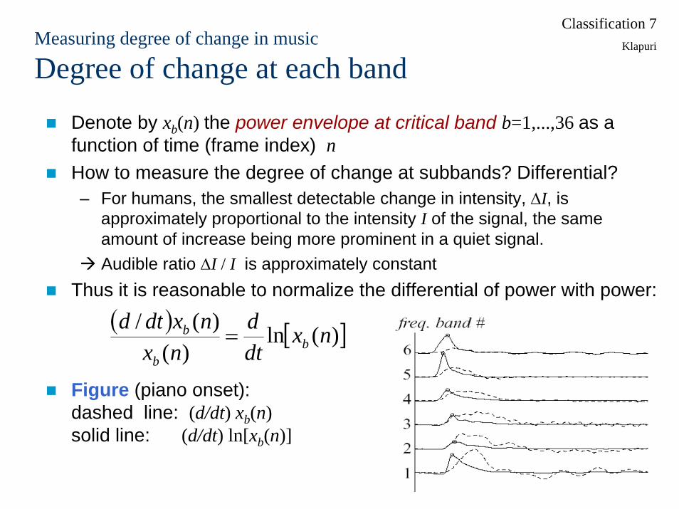
Degree of change at each band
Denote by xb(n) the power envelope at critical band b=1,...,36 as a function of time (frame index) nHow to measure the degree of change at subbands? Differential?– For humans, the smallest detectable change in intensity, ∆I, is
approximately proportional to the intensity I of the signal, the same amount of increase being more prominent in a quiet signal. Audible ratio ∆I / I is approximately constant
Thus it is reasonable to normalize the differential of power with power:
Figure (piano onset): dashed line: (d/dt) xb(n) solid line: (d/dt) ln[xb(n)]
( ) [ ])(ln)(
)(/ nxdtd
nxnxdtd
bb
b =

Classification 8KlapuriMeasuring degree of change in music
Degree of change at each bandA numerically robust way of calculating the logarithm is the µ-law compression,
constant µ determines the degree of compression for xb(n) (µ=10...104 / σx)Lowpass filter the compressed power envelopes at 10Hz– denote resulting signal with zb(n)
Differentiate, and retain only positive changes (HWR(x)=max(x, 0)):zb’(n) = HWR{zb(n)–zb(n–1)}
Form weighted sum of zb(n) and zb’(n):ub(n) = (1–λ) zb(n) + λ (fr/fLP) zb’(n)
where λ=0.8 (or 0.6...1.0) balances between zb(n) and zb’(n), and (fr/fLP) is a normalizing constant
( ) ( )[ ]( )µµ+
+=
1ln1ln nxny b
b

Classification 9KlapuriMeasuring degree of change in music
Degree of change at each band
Figure: illustration of the dynamic compression and weighted differentiation steps for an artificial subband signal xb(n)
x b(n
)u b
(n)

Classification 10KlapuriMeasuring degree of change in music
Summary
Finally: sum across channels to estimate overall change
Filterbank
Perceived change at subband Com
bine results
music signal
. . .
. . .output
∑=
=36
1)()(
bb nunv
powerenvelope
µ-law compress
lowpassfilter
d / dt,rectify
ub(n)xb(n)
v(n)
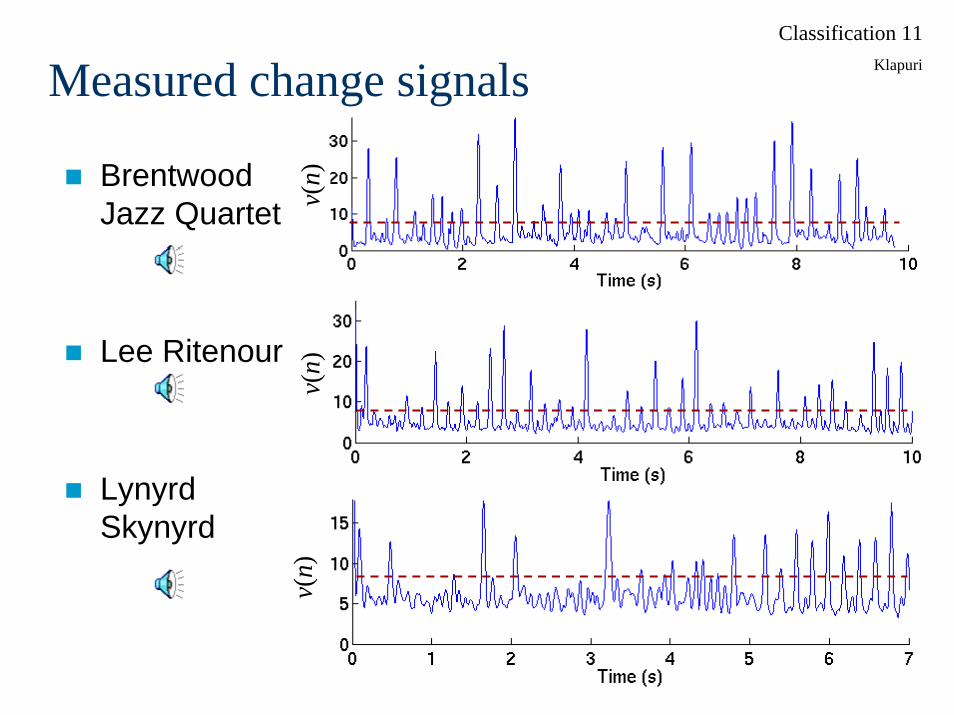
Classification 11KlapuriMeasured change signals
BrentwoodJazz Quartet
Lee Ritenour
Lynyrd Skynyrd
v(n)
v(n)
v(n)
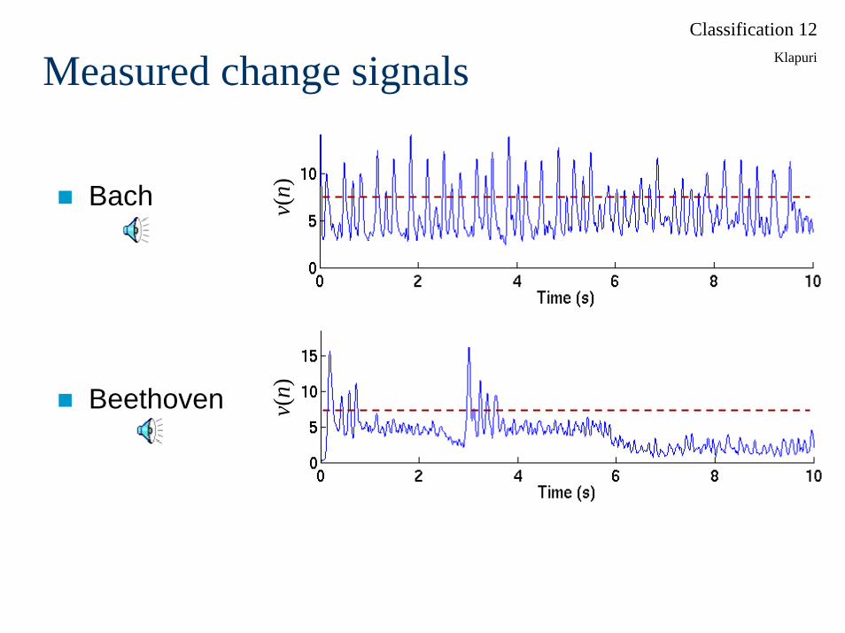
Classification 12KlapuriMeasured change signals
Bach
Beethoven v(n)
v(n)
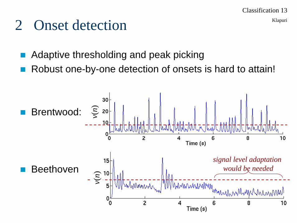
Classification 13Klapuri2 Onset detection
Adaptive thresholding and peak pickingRobust one-by-one detection of onsets is hard to attain!
Brentwood:
Beethovensignal level adaptation
would be needed
v(n)
v(n)
Classification 14KlapuriOnset detection
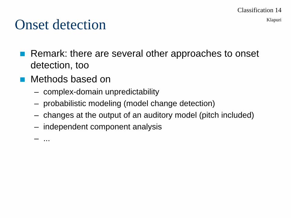
Remark: there are several other approaches to onset detection, tooMethods based on– complex-domain unpredictability– probabilistic modeling (model change detection)– changes at the output of an auditory model (pitch included)– independent component analysis– ...
Classification 15Klapuri3 Musical meter
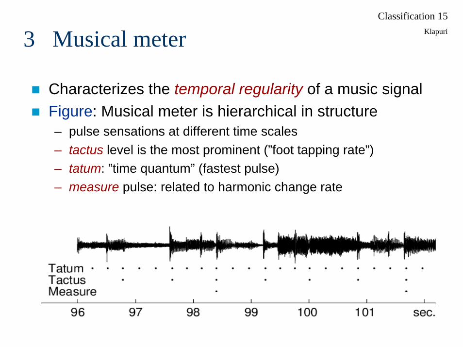
Characterizes the temporal regularity of a music signalFigure: Musical meter is hierarchical in structure– pulse sensations at different time scales– tactus level is the most prominent (”foot tapping rate”)– tatum: ”time quantum” (fastest pulse)– measure pulse: related to harmonic change rate
Classification 16KlapuriMeter analysis
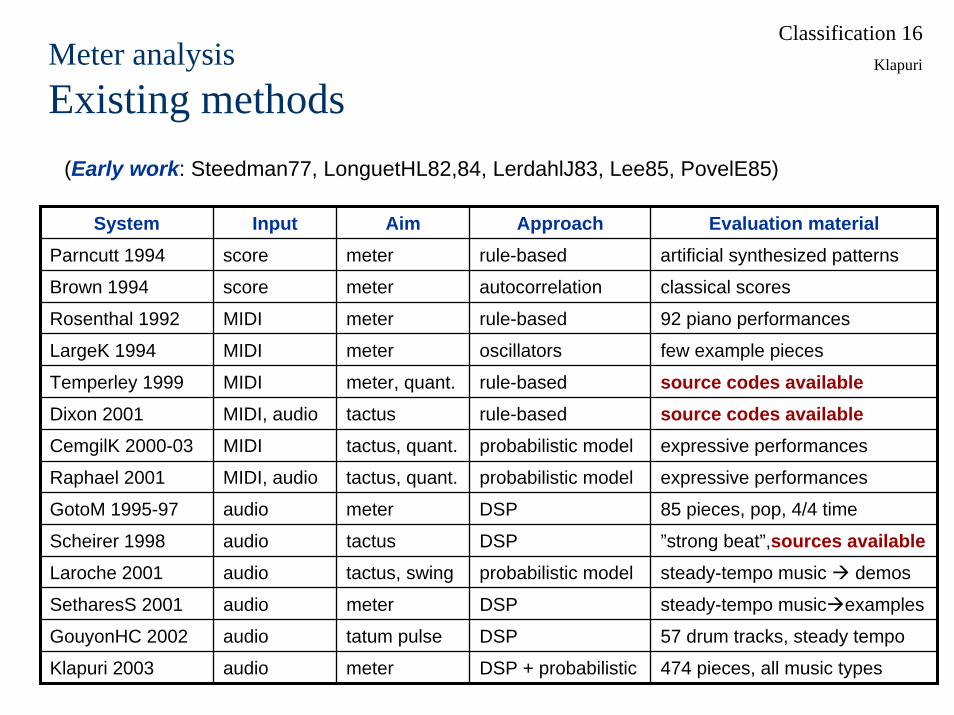
Existing methods(Early work: Steedman77, LonguetHL82,84, LerdahlJ83, Lee85, PovelE85)
System Input Aim Approach Evaluation materialParncutt 1994 score meter rule-based artificial synthesized patterns
classical scores
92 piano performances
few example pieces
source codes availablesource codes availableexpressive performances
expressive performances
85 pieces, pop, 4/4 time
”strong beat”,sources availablesteady-tempo music demos
steady-tempo music examples
57 drum tracks, steady tempo
474 pieces, all music types
Brown 1994 score meter autocorrelation
Rosenthal 1992 MIDI meter rule-based
LargeK 1994 MIDI meter oscillators
Temperley 1999 MIDI meter, quant. rule-based
Dixon 2001 MIDI, audio tactus rule-based
CemgilK 2000-03 MIDI tactus, quant. probabilistic model
Raphael 2001 MIDI, audio tactus, quant. probabilistic model
GotoM 1995-97 audio meter DSP
Scheirer 1998 audio tactus DSP
Laroche 2001 audio tactus, swing probabilistic model
SetharesS 2001 audio meter DSP
GouyonHC 2002 audio tatum pulse DSP
Klapuri 2003 audio meter DSP + probabilistic

Classification 17KlapuriMeter analysis
Overview of the TUT method
Classification 18KlapuriMeter analysis
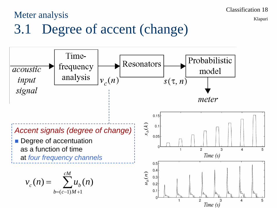
3.1 Degree of accent (change)
Accent signals (degree of change)Degree of accentuation as a function of time at four frequency channels
∑+−=
=cM
Mcbbc nunv1)1(
)()(

Classification 19KlapuriMeter analysis
3.2 Metrical pulse saliences
Metrical pulse saliences (weigths)Saliences of different metrical pulses τ at time n(resonator energies)
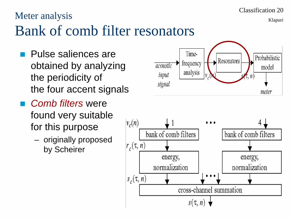
Classification 20KlapuriMeter analysis
Bank of comb filter resonatorsPulse saliences are obtained by analyzingthe periodicity ofthe four accent signalsComb filters werefound very suitablefor this purpose– originally proposed
by Scheirer
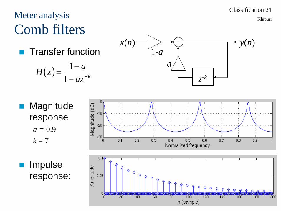
Classification 21KlapuriMeter analysis
Comb filtersx(n) y(n)
z-k
a1-aTransfer function
Magnituderesponsea = 0.9k = 7
Impulseresponse:
( ) kazazH −−
−=
11

Classification 22KlapuriMeter estimation
Bank of comb filter resonators
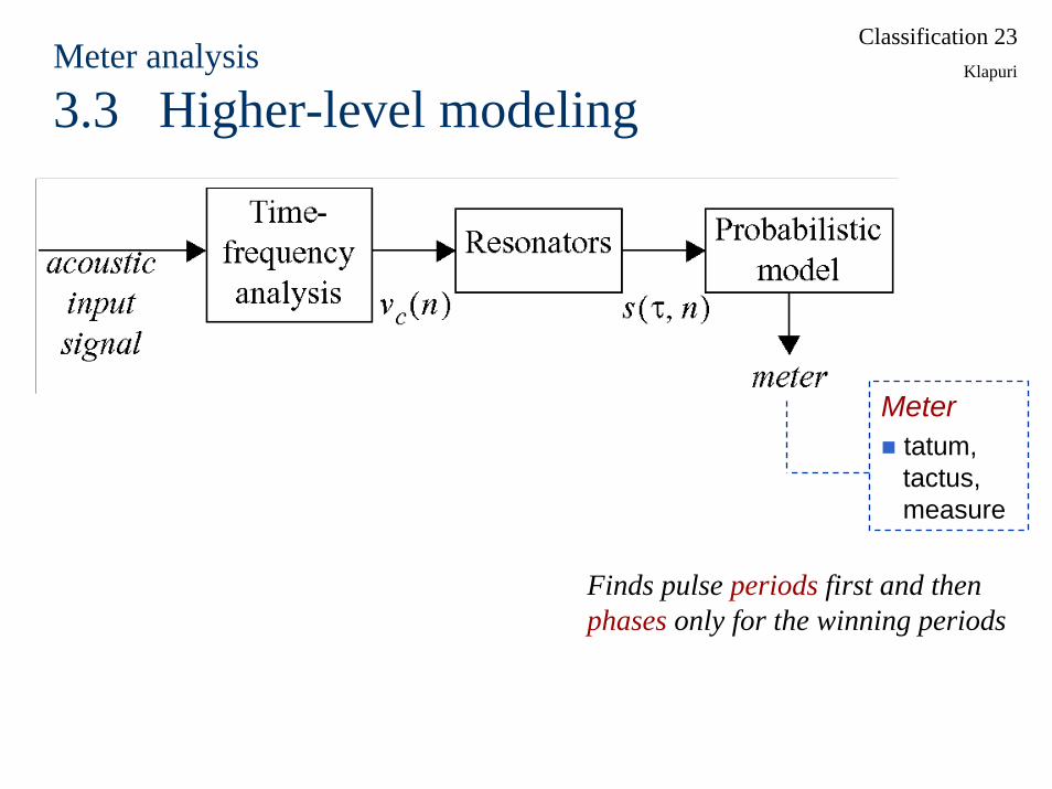
Classification 23KlapuriMeter analysis
3.3 Higher-level modeling
Metertatum,tactus,measure
Finds pulse periods first and then phases only for the winning periods

Classification 24Klapuri
Tactus:
Time
Observation:(comb filter energies)
Measure:
Tatum:
Pulse periodsHMM
Classification 25KlapuriMeter analysis
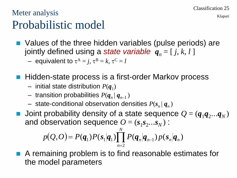
Probabilistic modelValues of the three hidden variables (pulse periods) are jointly defined using a state variable qn = [ j, k, l ]– equivalent to τA = j, τB = k, τC = l
Hidden-state process is a first-order Markov process– initial state distribution P(q1)– transition probabilities P(qn | qn–1 )– state-conditional observation densities P(sn | qn )
Joint probability density of a state sequence Q = (q1q2...qN )and observation sequence O = (s1s2...sN ) :
A remaining problem is to find reasonable estimates for the model parameters
( ) ∏=
−=N
nnnnn pPPPOQp
21111 )()()()(, qsqqqsq
Classification 26KlapuriMeter analysis
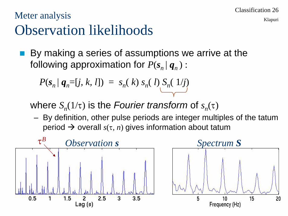
Observation likelihoodsBy making a series of assumptions we arrive at the following approximation for P(sn | qn ) :
P(sn | qn=[j, k, l]) = sn( k) sn( l) Sn( 1/j)
where Sn(1/τ) is the Fourier transform of sn(τ)– By definition, other pulse periods are integer multiples of the tatum
period overall s(τ, n) gives information about tatum
Observation sτB Spectrum S
Classification 27Klapuri
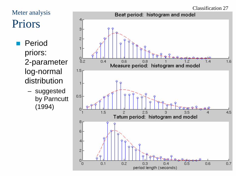
Meter analysis
PriorsPeriodpriors:2-parameterlog-normaldistribution– suggested
by Parncutt(1994)
Classification 28KlapuriMeter analysis
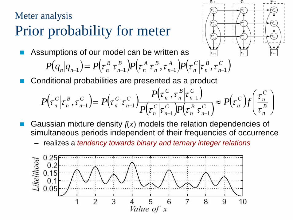
Prior probability for meterAssumptions of our model can be written as
Conditional probabilities are presented as a product
Gaussian mixture density f(x) models the relation dependencies of simultaneous periods independent of their frequencies of occurrence – realizes a tendency towards binary and ternary integer relations
( ) ( ) ( ) ( )Cn
Bn
Cn
An
Bn
An
Bn
Bnnn PPPqqP 1111 ,, −−−− = ττττττττ
( ) ( ) ( )( ) ( ) ( ) ⎟⎟
⎠
⎞⎜⎜⎝
⎛≈=
−−
−−− B
n
CnC
nCn
Bn
Cn
Cn
Cn
Bn
CnC
nCn
Cn
Bn
Cn fP
PPP
PPτττ
τττττττ
τττττ11
111
,,
Classification 29KlapuriMeter analysis
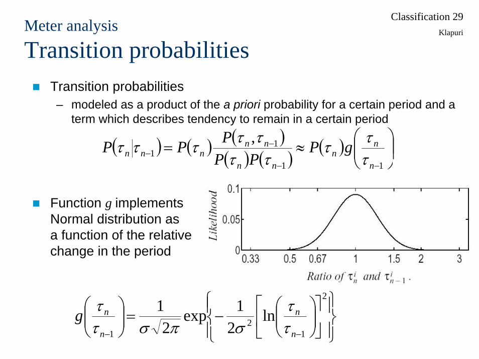
Transition probabilitiesTransition probabilities– modeled as a product of the a priori probability for a certain period and a
term which describes tendency to remain in a certain period
Function g implements Normal distribution as a function of the relative change in the period
( ) ( ) ( )( ) ( )
( ) ⎟⎟⎠
⎞⎜⎜⎝
⎛≈=
−−
−−
11
11
,n
nn
nn
nnnnn gP
PPPPP
τττ
τττττττ
⎪⎭
⎪⎬⎫
⎪⎩
⎪⎨⎧
⎥⎦
⎤⎢⎣
⎡⎟⎟⎠
⎞⎜⎜⎝
⎛−=⎟⎟
⎠
⎞⎜⎜⎝
⎛
−−
2
12
1
ln2
1exp2
1n
n
n
ngττ
σπσττ
Classification 30KlapuriMeter analysis
Finding state sequenceThe most likely sequence of meter estimates can be found using Viterbi algorithm– causal algorithm: meter estimate at time n is determined according
to the end-state of the best partial path at that time– noncausal meter estimates after seeing a complete sequence of
observations can be computed using backward decoding

Classification 31KlapuriPhase estimation (beat locations)
The model finds periods first and then the phases for the different levels of the meter– phase estimation is based on the last τ outputs of the resonator of
the winning period (i.e., the filter state)– probabilistic modeling for phase is very similar to that for period
estimation, but is estimated separately for beat/measure/tatum

Classification 32Klapuri
Meter analysis
Summary
Registral accent signalsDegree of accentuation (stress) as a function of time at four frequency channels Metrical pulse strengths
Strengths of different metrical pulses τ at time n(resonator energies)
Metertatum,tactus,measure
Classification 33KlapuriDemonstrations
http://www.cs.tut.fi/~klap/iiro/meter/


