SPECTRAL DATA FOR G-HIGGS BUNDLES
Laura P. Schaposnik M.New College
University of Oxford
A thesis submitted for the degree of
Doctor of Philosophy
August 2012


In memory of my mother,
Patricia Massolo.

Abstract
Spectral data for G-Higgs bundles
Laura P. Schaposnik M.New College
A thesis submitted for the degree of Doctor of Philosophy, Trinity Term 2012
This Thesis is dedicated to the study of principal G-Higgs bundles on a Riemann surface,
where G is a real form of a complex Lie group. The first three chapters of the thesis review
the theory of classical Higgs bundles and principal Higgs bundles. In Chapters 4-7 we
develop a new method of understanding G-Higgs bundles through their spectral data, for
G a split real form, G = SL(2,R), U(p, p), SU(p, p) and Sp(2p, 2p). Finally in Chapters 8-9
we give some open questions and applications of our results.
In particular, for G a split real form, we identify G-Higgs bundles with points of order
two in the regular fibres of the Gc Hitchin fibration in Chapter 4, where Gc is the complex-
ification of G. Through this approach, we study the special case of SL(2,R)-Higgs bundles,
for which we give an explicit description of the monodromy action in Chapter 5.
In the case of U(p, p)-Higgs bundles, in Chapter 6 we identify the known topological
invariants by the action of a natural involution at fixed points. Subsequently, we define the
spectral data in terms of the Jacobian variety of an intermediate curve, and for SU(p, p)-
Higgs bundles, in terms of the Prym variety of a quotient curve.
In Chapter 7 we study Sp(2p, 2p)-Higgs bundles and define their spectral data through
parabolic vector bundles in an intermediate cover of the Riemann surface. Through this
approach, we discover a rank 2 vector bundle moduli space in the fibres of the Sp(4p,C)
Hitchin fibration.
Lastly, in Chapter 9 we discuss further applications of our methods, among which are
implications concerning connectivity of moduli spaces of G-Higgs bundles, as well as non-
vanishing of higher cohomology groups of these moduli spaces.


Acknowledgements
First and foremost, I would like to thank my supervisor Nigel Hitchin. Working with him has
been a pleasure and during the last four years, our weekly meetings have been the great-
est source of inspiration and encouragement. I shall always be grateful for his enormous
support and patience, and his ability to make me excited about mathematics.
I am very thankful for the financial support I received from the Oxford University Press
and New College, through the joint Clarendon Award and Graduate Scholarship, and for
the grant received from the Centre for the Quantum Geometry of Moduli Spaces (QGM) in
Aarhus, which helped me to finish this thesis. I am also thankful to IHP in Paris, CRM in
Barcelona, and QGM in Aarhus for their hospitality during my research visits, and to the
Mathematics Departments in Cordoba, Buenos Aires and La Plata for their support.
Many mathematicians both in my department, and during research trips, have influ-
enced the way I understand maths, and I would like to thank all of them. In particular, I am
thankful to Tamas Hausel, Frances Kirwan, Peter Newstead and Jorge Solomin for inspir-
ing and helpful conversations, and to Alan Thompson, Jeff Giansiracusa, Bernardo Uribe,
Roberto Rubio and Steve Rayan for patiently explaining and discussing maths with me.
My time in Oxford would not have been the same without teaching mathematics. I am
greatly thankful to my college advisor Victor Flynn, who helped me to build my teaching
skills. The time I spent as a Lecturer at Hertford College and Magdalen College, and as a
Tutor at the Centre for International Education at Oxford, was most enjoyable.
I am grateful to my friends back at home and also to the ones I have made around the
world. Their amity has always been very important.
Finally, I am deeply thankful to my family for their support and encouragement, which
has kept me going throughout these years. I have always loved their physics at home. And
I would like to thank James Unwin, who saw this work be built from the first day. His love,
patience and confidence in my research has made me stronger each day.


Statement of Originality
This thesis contains no material that has already been accepted, or is concurrently being
submitted, for any degree or diploma or certificate or other qualification in this University
or elsewhere. To the best of my knowledge and belief this thesis contains no material
previously published or written by another person, except where due reference is made in
the text.
Laura P. Schaposnik M. August 28, 2012
ix

Contents
1 Overview and statement of results 1
2 Higgs bundles for complex Lie groups 9
2.1 Classical Higgs bundles . . . . . . . . . . . . . . . . . . . . . . . . . . . . . . . . . 9
2.1.1 Moduli space of vector bundles . . . . . . . . . . . . . . . . . . . . . . . . 10
2.1.2 Moduli space of Higgs bundles . . . . . . . . . . . . . . . . . . . . . . . . 11
2.2 Principal Higgs bundles . . . . . . . . . . . . . . . . . . . . . . . . . . . . . . . . . 18
2.2.1 Gc = SL(n,C) . . . . . . . . . . . . . . . . . . . . . . . . . . . . . . . . . . 19
2.2.2 Gc = Sp(2n,C) . . . . . . . . . . . . . . . . . . . . . . . . . . . . . . . . . . 20
2.2.3 Gc = SO(2n+ 1,C) . . . . . . . . . . . . . . . . . . . . . . . . . . . . . . . 22
2.2.4 Gc = SO(2n,C) . . . . . . . . . . . . . . . . . . . . . . . . . . . . . . . . . . 24
3 Higgs bundles for non-compact real forms 27
3.1 Higgs bundles for real forms . . . . . . . . . . . . . . . . . . . . . . . . . . . . . . 28
3.1.1 Real forms . . . . . . . . . . . . . . . . . . . . . . . . . . . . . . . . . . . . . 29
3.1.2 Higgs bundles for real forms . . . . . . . . . . . . . . . . . . . . . . . . . . 33
3.2 Real forms of SL(n,C) . . . . . . . . . . . . . . . . . . . . . . . . . . . . . . . . . . 38
3.2.1 G = SL(n,R) . . . . . . . . . . . . . . . . . . . . . . . . . . . . . . . . . . . 38
3.2.2 G = SU∗(2m) . . . . . . . . . . . . . . . . . . . . . . . . . . . . . . . . . . . 39
3.2.3 G = SU(p, q) . . . . . . . . . . . . . . . . . . . . . . . . . . . . . . . . . . . 41
xi
Contents
3.3 Real forms of SO(n,C) . . . . . . . . . . . . . . . . . . . . . . . . . . . . . . . . . . 43
3.3.1 G = SO(p, q) . . . . . . . . . . . . . . . . . . . . . . . . . . . . . . . . . . . 43
3.3.2 G = SO∗(2m) . . . . . . . . . . . . . . . . . . . . . . . . . . . . . . . . . . . 46
3.4 Real forms of Sp(2n,C) . . . . . . . . . . . . . . . . . . . . . . . . . . . . . . . . . 48
3.4.1 G = Sp(2n,R) . . . . . . . . . . . . . . . . . . . . . . . . . . . . . . . . . . 48
3.4.2 G = Sp(2p, 2q) . . . . . . . . . . . . . . . . . . . . . . . . . . . . . . . . . . 50
3.5 A geometric consequence . . . . . . . . . . . . . . . . . . . . . . . . . . . . . . . . 53
4 Higgs bundles for split real forms 55
4.1 An algebraic approach . . . . . . . . . . . . . . . . . . . . . . . . . . . . . . . . . . 55
4.1.1 Three dimensional subalgebras . . . . . . . . . . . . . . . . . . . . . . . . 56
4.1.2 Compact real structure . . . . . . . . . . . . . . . . . . . . . . . . . . . . . 59
4.1.3 A natural involution on Lie algebras . . . . . . . . . . . . . . . . . . . . . 60
4.1.4 The Kostant slice . . . . . . . . . . . . . . . . . . . . . . . . . . . . . . . . . 63
4.2 The Hitchin fibration . . . . . . . . . . . . . . . . . . . . . . . . . . . . . . . . . . . 65
4.2.1 The Teichmüller component . . . . . . . . . . . . . . . . . . . . . . . . . . 65
4.2.2 Principal Higgs bundles and split real forms . . . . . . . . . . . . . . . . 66
5 Monodromy of the SL(2,R) Hitchin fibration Hitchin fibration 69
5.1 The SL(2,C) Hitchin fibration . . . . . . . . . . . . . . . . . . . . . . . . . . . . . 70
5.1.1 The regular fibres of the Hitchin fibration . . . . . . . . . . . . . . . . . 70
5.1.2 The involution Θ . . . . . . . . . . . . . . . . . . . . . . . . . . . . . . . . . 71
5.2 The monodromy action . . . . . . . . . . . . . . . . . . . . . . . . . . . . . . . . . 73
5.2.1 Gauss-Manin connection . . . . . . . . . . . . . . . . . . . . . . . . . . . . 73
5.2.2 A combinatorial approach to monodromy for SL(2,C) . . . . . . . . . . 74
5.2.3 The fixed points of Θ : (E,Φ) 7→ (E,−Φ) . . . . . . . . . . . . . . . . . . 79
5.3 The SL(2,R) moduli space . . . . . . . . . . . . . . . . . . . . . . . . . . . . . . . 81
5.3.1 The action on Z2[E] . . . . . . . . . . . . . . . . . . . . . . . . . . . . . . . 81
xii

Contents
5.3.2 The representation of G1 . . . . . . . . . . . . . . . . . . . . . . . . . . . . 88
5.3.3 The monodromy action of π1(Areg) on P[2] . . . . . . . . . . . . . . . 92
6 Spectral data for U(p, p)-Higgs bundles 95
6.1 U(p, p)-Higgs bundles . . . . . . . . . . . . . . . . . . . . . . . . . . . . . . . . . . 96
6.1.1 The spectral curves . . . . . . . . . . . . . . . . . . . . . . . . . . . . . . . 97
6.2 The spectral data of U(p, p)-Higgs bundles . . . . . . . . . . . . . . . . . . . . . 98
6.2.1 The associated invariants . . . . . . . . . . . . . . . . . . . . . . . . . . . . 102
6.3 The spectral data of SU(p, p)-Higgs bundles . . . . . . . . . . . . . . . . . . . . . 109
6.3.1 The condition ΛpV ∼= ΛpW ∗ . . . . . . . . . . . . . . . . . . . . . . . . . . 109
7 Spectral data for Sp(2p, 2p)-Higgs bundles 111
7.1 Sp(2p, 2p)-Higgs bundles . . . . . . . . . . . . . . . . . . . . . . . . . . . . . . . . 112
7.1.1 The associated curves . . . . . . . . . . . . . . . . . . . . . . . . . . . . . . 113
7.2 The spectral data of Sp(2p, 2p)-Higgs bundles . . . . . . . . . . . . . . . . . . . 117
7.2.1 Stability conditions . . . . . . . . . . . . . . . . . . . . . . . . . . . . . . . 125
7.2.2 Dimensional calculations via the spectral data . . . . . . . . . . . . . . . 126
8 Applications 131
8.1 The moduli space of SL(2,R)-Higgs bundles . . . . . . . . . . . . . . . . . . . . 131
8.1.1 The orbits of the monodromy action . . . . . . . . . . . . . . . . . . . . . 132
8.1.2 Connected components ofMSL(2,R) . . . . . . . . . . . . . . . . . . . . . 133
8.2 The moduli space of U(p, p)-Higgs bundles . . . . . . . . . . . . . . . . . . . . . 137
8.2.1 Connected components ofMU(p,p) . . . . . . . . . . . . . . . . . . . . . . 138
8.2.2 Connected components ofMSU(p,p) . . . . . . . . . . . . . . . . . . . . . 141
8.3 The moduli space of Sp(2p, 2p)-Higgs bundles . . . . . . . . . . . . . . . . . . . 142
8.3.1 Parabolic vector bundles on S . . . . . . . . . . . . . . . . . . . . . . . . . 142
8.3.2 Connectivity ofMSp(2p,2p) . . . . . . . . . . . . . . . . . . . . . . . . . . . 143
xiii

Contents
9 Further questions 145
9.1 Connectivity ofMG . . . . . . . . . . . . . . . . . . . . . . . . . . . . . . . . . . . . 145
9.2 Cohomology groups ofMG . . . . . . . . . . . . . . . . . . . . . . . . . . . . . . . 146
9.3 Spectral data for other real forms . . . . . . . . . . . . . . . . . . . . . . . . . . . 147
Bibliography 151
xiv

Chapter 1
Overview and statement of results
Since Higgs bundles were introduced in 1987 [Hit87], they have found applications in
many areas of mathematics and mathematical physics. In particular, Hitchin showed in
[Hit87] that their moduli spaces give examples of Hyper-Kähler manifolds and that they
provide an interesting example of integrable systems [Hit87a]. More recently, Hausel and
Thaddeus [HT03] related Higgs bundles to mirror symmetry, and in the work of Kapustin
and Witten [KW07] Higgs bundles were used to give a physical derivation of the geometric
Langlands correspondence.
The moduli spaceMG of polystable G-Higgs bundles over a compact Riemann surface
Σ, for G a real form of a complex semisimple Lie group Gc , may be identified through
non-abelian Hodge theory with the moduli space of representations of the fundamental
group of Σ (or certain central extension of the fundamental group) into G (see [G-PGM09]
for the Hitchin-Kobayashi correspondence for G-Higgs bundles). Motivated partially by this
identification, the moduli space of G-Higgs bundles has been studied by various researchers,
mainly through a Morse theoretic approach (see, for example, [BW12] for an expository
article on applications of Morse theory to moduli spaces of Higgs bundles).
Real forms of SL(n,C) and GL(n,C) were initially considered in [Hit87] and [Hit92],
where Hitchin studied SL(2,R)-Higgs bundles, and later on extended those results to
1
Chapter 1. Overview and statement of results
SL(n,R)-Higgs bundles. Connectivity of the moduli space of G-Higgs bundles for the real
forms G = PGL(n,R), PGL(2,R), SU(p, q) and PU(p, p) was studied by Bradlow, Gothen,
Garcia Prada and Oliveira ( e.g., [BG-PG03], [BG-PG04], [Ol10]), as well as by Xia and
Markman [MX02, Xia97, Xia00, Xia03], their main results holding under certain constraints
on the degrees of the vector bundles involved. Finally, Garcia Prada and Oliveira calculated
the connected components for U∗(2n)-Higgs bundles in [G-PO10].
In the case of real forms of Sp(2n,C), at the time of writing this thesis, only the group
Sp(2n,R) has been considered. Gothen studied real symplectic rank 4 Higgs bundles in
[G95], and together with Bradlow and Garcia-Prada studied connectivity for Sp(2n,R)-
Higgs bundles for arbitrary n (e.g. [BG-PG11]). The study of connected components for
the particular case of Sp(4,R) has received extensive attention from Gothen, Garcia Prada,
Mundet and Oliveira (among others, see [BG-PG03], [G-PGM08]).
Finally, G-Higgs bundles for G a real form of SO(2n + 1,C) or SO(2n,C) have been
studied by Aparicio and Garcia Prada in [Ap09] and [ApG-P10], where connectivity results
are given for SO0(p, q)-Higgs bundles for p = 1 and q odd, and by Bradlow, Gothen and
Garcia Prada in [BG-PG06], where connected components for SO∗(2n)-Higgs bundle are
given for maximal topological invariant.
This thesis is dedicated to the study of principal G-Higgs bundles and their moduli
spaces, for G a real form of a complex Lie group Gc . After introducing the background
material needed in Chapter 2 and Chapter 3, we concentrate our attention on the case of
G being a split real form in general, and on the particular cases of G = SL(2,R), U(p, p),
SU(p, p) and Sp(2p, 2p). The original results and new methods developed in this thesis ap-
pear in Chapters 4-8, whilst further applications are given in Chapter 9. We have organised
the work in the following way.
2
We begin Chapter 2 by introducing classical Higgs bundles and principal Gc-Higgs bun-
dles for a complex Lie group Gc , following [Hit87] and [Hit87a]. Then, via the Hitchin
fibration, the spectral data approach considered in [Hit07] is presented, and a detailed
description of the method is given for the classical Lie groups Gc = GL(n,C), SL(n,C),
Sp(2p,C), SO(2n,C) and SO(2n+ 1,C).
In Chapter 3 we recall the main properties of principal G-Higgs bundles for a real form
G of a complex Lie group Gc , describing both the Lie theoretic construction of Higgs bun-
dles as well as their appearance as fixed points of a certain involution on the moduli space
of Gc-Higgs bundles. In preparation for the study of the spectral data of G-Higgs bundles,
and since we know of no complete list, in this chapter we give a thorough description of G-
Higgs bundles when the structure group is a non-compact real form of a classical complex
Lie group. In particular, in each case we describe the involution defining the corresponding
G-Higgs bundle, and study the associated ring of invariant polynomials.
In Chapter 4 we study G-Higgs bundles for G a split real form. In this case, the Hitchin
map is surjective and so the generic fibre is a torus. Moreover, the Teichmüller component
defined in [Hit92] provides an origin for the bundles of the same topological type, and
makes the fibre an abelian variety. It is via the Teichmüller component that we are able
to describe the moduli space of G-Higgs bundles as fixed points in the moduli space of
Gc-Higgs bundles:
Theorem 4.12. The intersection of the subspace of the Higgs bundle moduli spaceMGc corre-
sponding to the split real form of gc with the smooth fibres of the Hitchin fibration
h : MGc →AGc ,
is given by the elements of order two in those fibres.
3

Chapter 1. Overview and statement of results
As a consequence, this moduli space is a finite covering of an open set in the base.
Hence, in the case of a split real form G, the natural way of understanding the topology
of the moduli space of G-Higgs bundles is via the monodromy of the covering. Although
generally this is known to be a very difficult problem, the case of rank-2 Higgs bundles is
considerably more tenable.
In Chapter 5 we study SL(2,R)-Higgs bundles. Through Theorem 4.12, the moduli
space can be seen as points of order two in the classical Hitchin fibration. We use the
results of Copeland [Cop05] to understand the generators of the monodromy action for
SL(2,R)-Higgs bundles, and obtain an explicit description of the monodromy action:
Theorem 5.23. The monodromy action on the first mod 2 cohomology of the fibres of the
Hitchin fibration is given by the group of matrices acting on Z6g−62 of the form
I2g A
0 π
, (1.1)
where
• π is the quotient action on Z4g−52 /(1, · · · , 1) induced by the permutation action of the
symmetric group S4g−4 on Z4g−52 ;
• A is any (2g)× (4g − 6) matrix with entries in Z2.
The monodromy approach appeared to be very difficult to follow for higher rank Higgs
bundles, and already for rank-3 Higgs bundles calculations using similar ideas to the rank-2
case did not lead to fruitful results. In order to study higher rank Higgs bundles for non-
split real forms, in Chapter 6 we look at the particular case of U(p, p)-Higgs bundles. As in
the case of complex Lie groups, we consider the characteristic polynomial p(x) of a U(p, p)-
Higgs bundle and the curve it defines. Extending the spectral data methods introduced in
4
Chapter 2, we obtain a description of the spectral data associated to U(p, p)-Higgs bundles:
Theorem 6.9. There is a one to one correspondence between U(p, p)-Higgs bundles (V⊕W,Φ)
on a compact Riemann surface Σ of genus g > 1 for which deg V > deg W, as given in
Definition 6.1, which have non-singular spectral curve, and triples (S, U1, D) where
• ρ : S→ Σ is a non-singular p-fold cover of Σ given by the equation
p(ξ) = ξp + a1ξp−1+ . . .+ ap−1ξ+ ap = 0
for ai ∈ H0(Σ, K2i) and ξ the tautological section of ρ∗K2;
• U1 is a line bundle on S whose degree is
deg U1 = deg V + (2p2− 2p)(g − 1);
• D is a positive subdivisor of the divisor of ap of degree m= deg W −deg V + 2p(g − 1).
The above approach relies heavily on the existence of a non singular locus in the
GL(2p,C) Hitchin base defining a smooth curve S associated to a U(p, p)-Higgs bundle.
For groups where this locus is empty, a different construction needs to be made. In Chapter
7 we study the case of Sp(2p, 2p)-Higgs bundles, for which we show that the character-
istic equations always define a reducible spectral curve. In this case, it is via the square
root of the characteristic polynomial P(x) := p2(x) that we obtain the spectral data of
Sp(2p, 2p)-Higgs bundles:
Theorem 7.10. Each stable Sp(2p, 2p)-Higgs bundle (E = V ⊕W,Φ) on a compact Riemann
surface Σ of genus g ≥ 2 for which p(η2) = 0 defines a smooth curve, has an associated pair
(S, M) where
(a) the curve ρ : S→ Σ is a smooth 2p-fold cover of Σ given by the equation
p(η2) = η2p + b1η2p−2+ . . .+ bp−1η
2+ bp = 0,
5
Chapter 1. Overview and statement of results
in the total space of K, where bi ∈ H0(Σ, K2i), and η is the tautological section of ρ∗K.
The curve S has a natural involution σ acting by η 7→ −η;
(b) the vector bundle M is a rank 2 vector bundle on the smooth curve ρ : S → Σ with
determinant bundle Λ2M ∼= ρ∗K−2p+1, and such that σ∗M ∼= M. Over the fixed points
of the involution, the vector bundle M is acted on by σ with eigenvalues +1 and −1.
Conversely, a pair (S, M) satisfying (a) and (b) induces a stable Sp(2p, 2p)-Higgs bundle
(ρ∗M = V ⊕W,Φ) on the compact Riemann surface Σ.
The intention of the preceding chapters is to provide a new approach to study the
topology of moduli spaces of flat G-bundles through the analysis of G-Higgs bundles. Since
the discriminant locus depends on the complex structure, it is very likely that the fixed point
locus intersects a generic fibre. In an attempt to show the utility of this new approach, in
Chapter 8 we give some applications of the results which appear in Chapters 4-7. Using
the results of Chapters 4-5, we can calculate the number of connected components of the
moduli space of SL(2,R)-Higgs bundles:
Proposition 8.5. The number of connected components of the moduli space of semistable
SL(2,R)-Higgs bundles is 2 · 22g + 2g − 3.
In the case of U(p, p)-Higgs bundles, we use the associated spectral data to describe the
connected components of the moduli space MU(p,p) which intersect regular fibres of the
classical Hitchin fibration:
Proposition 8.12. For each fixed invariant m as given in Proposition 6.4, the invariant
0 ≤ m < 2p(g − 1) labels exactly one connected component of MU(p,p) which intersects the
non-singular fibres of the Hitchin fibration
MGL(2p,C)→AGL(2p,C),
6
given by the fibration of α∗Jac(S) over a Zariski open set in
E ⊕p−1⊕
i=1
H0(Σ, K2i),
for E the total space of a vector bundle over a symmetric product as defined in Section 8.2.1.
In the case of Sp(2p, 2p)-Higgs bundles, we can describe the spectral data through the
results of [AG06] in terms of parabolic vector bundles, and analyse connectivity via the
work of Nitsure [N86]. In particular, we have the following results:
Proposition 8.19. There is exactly one connected component of the moduli spaceMSp(2p,2p)
which intersects the regular fibres of the Sp(4p,C) Hitchin fibration, and it is given by the
fibration of a Zariski open set in P sa , over a Zariski open set in the space
p⊕
i=1
H0(Σ, K2i),
whereP sa is the set of admissible rank 2 parabolic vector bundles on a quotient curve as defined
in Subsection 8.3.1.
Since many paths have been opened by the spectral data study of G-Higgs bundles, we
dedicate Chapter 9 to outline a number of interesting questions that could be approached
using the spectral data of real Higgs bundles. In particular, we conjecture the following:
Conjecture 9.1. For G = U(p, p), SU(p, p) and Sp(2p, 2p), any component of the fixed
point set of the involution ΘG , as defined in Section 3.1.2, intersects the so-called generic fibre
of the Hitchin fibrationMGc →AGc .
Among other things, this would imply that the connectivity results given in Chapter 8
do in fact realise all components of the moduli spacesMG . In Section 9.2 we discuss how
the methods developed in this thesis provide a new way of obtaining information about
7

Chapter 1. Overview and statement of results
the higher cohomology groups of the moduli spacesMG . Finally, in Section 9.3 we give an
insight into how the spectral data approach could be extended to other real forms.
8

Chapter 2
Higgs bundles for complex Lie
groups
In this Chapter we introduce classical Higgs bundles and then study principal Gc-Higgs
bundles for complex semisimple Lie groups Gc . We begin with an introduction to the sub-
ject following [Hit87, Hit87a], and in subsequent sections we study Gc-Higgs bundles for
Gc = SL(n,C), Sp(n,C), SO(2n+ 1,C) and SO(2n,C). In each case, we give a description
of the corresponding invariant polynomials, the Hitchin fibration and the associated spec-
tral curve. Following [Hit87a] and [Hit07], we describe the generic fibres of the Hitchin
fibration in terms of an associated spectral curve and a line bundle on it. We shall continue
to follow this approach in Chapter 6 and Chapter 7.
2.1 Classical Higgs bundles
We devote this section to developing the general theory of Higgs bundles. More details can
be found in [Hit87], [Hit87a], [D87], [Cor88], [S88], [N91] and [S92].
9
Chapter 2. Higgs bundles for complex Lie groups
2.1.1 Moduli space of vector bundles
Holomorphic vector bundles on a compact Riemann surface Σ of genus g ≥ 2 are topologi-
cally classified by their rank n and degree d.
Definition 2.1. The slope of a holomorphic vector bundle E on Σ is given by
µ(E) :=deg(E)rk(E)
.
A vector bundle E is said to be
• stable if for any proper, non-zero sub-bundle F ⊂ E we have µ(F)< µ(E);
• semi-stable if for any proper, non-zero sub-bundle F ⊂ E we have the inequality
µ(F)≤ µ(E);
• polystable if it is a direct sum of stable bundles all of which have the same slope.
It is known that the space of holomorphic bundles of fixed rank and fixed degree, up to
isomorphism, is not a Hausdorff space. However, through Mumford’s Geometric Invariant
Theory one can construct the moduli space N (n, d) of stable bundles of fixed rank n and
degree d, which has the natural structure of an algebraic variety.
Theorem 2.2. For coprime n and d, the moduli spaceN (n, d) is a smooth projective algebraic
variety of dimension n2(g − 1) + 1.
Remark 2.3. All line bundles are stable, and thus N (1, d) contains all line bundles of degree
d, and is isomorphic to the Jacobian Jacd(Σ) of Σ, an abelian variety of dimension g.
Let Gc be a complex semisimple Lie group. Following [Ra75] we define stability for
principal Gc-bundles as follows (the reader should refer to [Ap09, Section 1.1] for a de-
tailed description of the definition below).
10
2.1. Classical Higgs bundles
Definition 2.4. A holomorphic principal Gc-bundle P → Σ is said to be stable (respectively
semi-stable) if for every reduction σ : Σ→ P/Q to maximal parabolic subgroups Q of Gc we
have
degσ∗Trel > 0 ( resp. ≥ 0 ),
where Trel denotes the relative tangent bundle for the projection P/Q→ Σ.
The notion of polystability may be carried over to principal Gc-bundles, allowing one to
construct the moduli space of polystable principal Gc-bundles of fixed topological type over
the compact Riemann surface Σ.
2.1.2 Moduli space of Higgs bundles
Classically, a Higgs bundle on the compact Riemann surface Σ is defined as follows.
Definition 2.5. A Higgs bundle is a pair (E,Φ) for E a holomorphic vector bundle on Σ, and
Φ a section in H0(Σ, End(E)⊗ K). The map Φ is called the Higgs field.
A vector subbundle F of E for which Φ(F)⊂ F ⊗K is said to be a Φ-invariant subbundle
of E. Stability for Higgs bundles is defined in terms of Φ-invariant subbundles:
Definition 2.6. A Higgs bundle (E,Φ) is
• stable if for each proper Φ-invariant subbundle F one has µ(F)< µ(E);
• semi-stable if for each Φ-invariant subbundle F one has µ(F)≤ µ(E);
• polystable if (E,Φ) = (E1,Φ1)⊕ (E2,Φ2)⊕ . . .⊕ (Er ,Φr), where (Ei ,Φi) is stable with
µ(Ei) = µ(E) for all i.
Example 2.7. For the Riemann surface Σ of genus g > 1, choose a square root K1/2 of the
canonical bundle K, and a section ω of K2. Consider E = K12 ⊕ K−
12 . Then, the Higgs bundle
11
Chapter 2. Higgs bundles for complex Lie groups
(E,Φ) for Φ given by
Φ =
0 ω
1 0
∈ H0(Σ, EndE ⊗ K)
is stable. In fact, since K12 is not Φ-invariant, there are no subbundles of positive degree
preserved by Φ.
Stable Higgs bundles satisfy many interesting properties. Among others, one should
note that if a Higgs bundle (E,Φ) is stable, then for λ ∈ C∗ and α a holomorphic automor-
phism of E, the induced Higgs bundles (E,λΦ) and (E,α∗Φ) are stable.
Definition 2.8. A Gc-Higgs bundle is a pair (P,Φ) where P is a principal Gc-bundle over
Σ, and the Higgs field Φ is a holomorphic section of the vector bundle adP ⊗C K, for adP the
vector bundle associated to the adjoint representation.
Example 2.9. Note that in Example 2.7, the Higgs bundle (E,Φ) has traceless Higgs field,
and the determinant bundle Λ2E is trivial. Hence, (E,Φ) is an example of an SL(2,C)-Higgs
bundle.
When Gc ⊂ GL(n,C), a Gc-Higgs bundle gives rise to a Higgs bundle in the classical
sense, in general with some extra structure reflecting the definition of Gc . Note that classical
Higgs bundles are given by GL(n,C)-Higgs bundles.
In order to define the moduli space of classical Higgs bundles, we shall first define
an appropriate equivalence relation. For this, consider a strictly semi-stable Higgs bundle
(E,Φ). As it is not stable, E admits a subbundle F ⊂ E of the same slope which is preserved
by Φ. If F is a subbundle of E of least rank and same slope which is preserved by Φ, it
follows that F is stable and hence the induced pair (F,Φ) is stable. Then, by induction one
obtains a flag of subbundles
F0 = 0⊂ F1 ⊂ . . .⊂ Fr = E
12
2.1. Classical Higgs bundles
where µ(Fi/Fi−1) = µ(E) for 1≤ i ≤ r, and where the induced Higgs bundles (Fi/Fi−1,Φi)
are stable. This is the Jordan-Hölder filtration of E, and it is not unique. However, the
graded object
Gr(E,Φ) :=r⊕
i=1
(Fi/Fi=1,Φi)
is unique up to isomorphism.
Definition 2.10. Two semi-stable Higgs bundles (E,Φ) and (E′,Φ′) are said to be S-equivalent
if Gr(E,Φ)∼= Gr(E′,Φ′).
Remark 2.11. If a pair (E,Φ) is strictly stable, then the induced Jordan-Hölder filtration
is trivial, and so the isomorphism class of the graded object is the isomorphism class of the
original pair.
From [N91, Theorem 5.10]we letM (n, d) be the moduli space of S-equivalence classes
of semi-stable Higgs bundles of fixed degree d and fixed rank n. The moduli spaceM (n, d)
is a quasi-projective scheme, and has an open subscheme M ′(n, d) which is the moduli
scheme of stable pairs. Thus every point is represented by either a stable or a polystable
Higgs bundle. When d and n are coprime, the moduli space M (n, d) is smooth. The
cotangent space of N (n, d) over the stable locus is contained inM (n, d) as a Zariski open
subset. The moduli spaceM (n, d) is a non-compact variety which has complex dimension
2n2(g − 1) + 2. Moreover, it is a hyperkähler manifold with natural symplectic form ω de-
fined on the infinitesimal deformations (A, Φ) of a Higgs bundle (E,Φ), for A∈ Ω01(End0E)
and Φ ∈ Ω10(End0E), by
ω((A1, Φ1), (A2, Φ2)) =
∫
Σtr(A1Φ2− A2Φ1) (2.1)
(see [Hit87],[Hit87a] for details). For simplicity, we shall fix n and d and write M for
M (n, d).
By extending the stability definitions for principal Gc-bundles, one can define stable,
13
Chapter 2. Higgs bundles for complex Lie groups
semi-stable and pol ystable Gc-Higgs bundles. Moreover, by reducing to parabolic sub-
groups one can define the corresponding moduli space for Gc-Higgs bundles (for details
about the corresponding constructions, the reader should refer to, e.g., [BiGo08, Section
3], [Ap09, Section 1]):
Definition 2.12. We denote byMGc the moduli space of polystable Gc-Higgs bundles.
We shall denote by pi , for i = 1, . . . , k, a homogeneous basis for the algebra of invariant
polynomials on the Lie algebra gc of Gc , and let di be their degrees. Following [Hit87a],
the Hitchin fibration is given by
h : MGc −→ AGc :=k⊕
i=1
H0(Σ, Kdi ), (2.2)
(E,Φ) 7→ (p1(Φ), . . . , pk(Φ)). (2.3)
The map h is referred to as the Hitchin map, and is a proper map for any choice of basis
(see [Hit87a, Section 4] for details). Furthermore, the dimension of the vector space AGc
always satisfies
dimAGc = dimMGc/2,
and the Hitchin map makes the Higgs bundle moduli space into an integrable system. When
the group Gc being considered is implicit, we shall drop the subscript Gc and refer to the
moduli spaceM and the Hitchin baseA .
In the remainder of this Section, following [Hit07], we shall describe the generic fi-
bres of the Hitchin fibration for classical Higgs bundles. Then, in Section 2.2 we describe
the generic fibres in the case of Gc-Higgs bundles for the classical groups Gc = SL(n,C),
Sp(2n,C), SO(2n+ 1,C) and SO(2n,C).
As before, let K be the canonical bundle of Σ, and X its total space with projection
ρ : X → Σ. We shall denote by η the tautological section of the pull back ρ∗K on X , and
abusing notation we denote with the same symbols the sections of powers K i on Σ and
14

2.1. Classical Higgs bundles
their pull backs to X . Consider a smooth curve S in X with equation
ηn+ a1ηn−1+ a2η
n−2+ . . .+ an−1η+ an = 0, (2.4)
for ai ∈ H0(Σ, K i). By the adjunction formula on X , since the canonical bundle K has trivial
cotangent bundle one has KS∼= ρ∗Kn, and hence
gS = 1+ n2(g − 1).
Starting with a line bundle M on the smooth curve ρ : S→ Σ with equation as in (2.4), we
shall obtain a classical Higgs bundle by considering the direct image ρ∗M of M . Recall that
by definition of direct image, given an open set U ⊂ Σ, one has
H0(ρ−1(U ), M) = H0(U ,ρ∗M). (2.5)
Multiplication by the the tautological section η induces the map
H0(ρ−1(U ), M)η // H0(ρ−1(U ), M ⊗ρ∗K).
From (2.5) this map can be pushed down to obtain
Φ : ρ∗M // ρ∗M ⊗ K ,
defining a Higgs field Φ ∈ H0(Σ, EndE ⊗ K) for E := ρ∗M . From Grothendieck-Riemann-
Roch, one has degE = degM + (n2 − n)(1 − g). Moreover, the Higgs field satisfies its
characteristic equation, which by construction is
ηn+ a1ηn−1+ a2η
n−2+ . . .+ an−1η+ an = 0.
15

Chapter 2. Higgs bundles for complex Lie groups
Since Φ satisfies the above equation, η gives an eigenvalue of Φ. The characteristic polyno-
mial of Φ restricted to an invariant subbundle would divide the characteristic polynomial
of Φ. Since S is smooth, it is irreducible, and thus there are no invariant subbundles of the
Higgs field. Hence, the induced Higgs bundle (E,Φ) is stable. Recall that the Norm map
Nm : Pic(S)→ Pic(Σ),
associated to ρ, is defined on divisor classes by Nm(∑
ni pi) =∑
niρ(pi). The kernel of the
Norm map is the Prym variety, and is denoted by Prym(S,Σ). From [BNR, Section 4] the
determinant bundle of M satisfies
Λnρ∗M ∼= Nm(M)⊗ K−n(n−1)/2.
For V ⊂ S an open set, we have V ⊂ ρ−1(ρ(V )) and hence a natural restriction map
H0(ρ−1(ρ(V )), M)→ H0(V , M),
which gives the evaluation map ev : ρ∗ρ∗M → M . Multiplication by η commutes with this
linear map and so the action of ρ∗Φ on the dual of the vector bundle ρ∗ρ∗M preserves a
one-dimensional subspace. Hence M∗ is an eigenspace of ρ∗Φt , with eigenvalue η. Equiv-
alently, M is the cokernel of ρ∗Φ− η acting on ρ∗E ⊗ ρ∗K∗. By means of the Norm map,
this correspondence can be seen on the curve S via the exact sequence
0 // M ⊗ρ∗K1−n // ρ∗Eρ∗Φ−η// ρ∗(E ⊗ K) ev // M ⊗ρ∗K // 0 , (2.6)
and its dualised sequence
0 // M∗⊗ρ∗K∗ // ρ∗(E∗⊗ K∗) // ρ∗E∗ // M∗⊗ρ∗Kn−1 // 0 . (2.7)
16

2.1. Classical Higgs bundles
In particular, from the relative duality theorem one has that
ρ∗(M)∗ ∼= ρ∗(KS ⊗ρ∗K−1⊗M∗), (2.8)
and thus E∗ is the direct image sheaf ρ∗(M∗⊗ρ∗Kn−1).
Conversely, let (E,Φ) be a classical Higgs bundle. The characteristic polynomial is
det(x −Φ) = xn+ a1 xn−1+ a2 xn−2+ . . .+ an−1 x + an.
The coefficients of the above polynomial define the spect ral curve S of the Higgs bundle
(E,Φ) in the total space X . The equation of S is as (2.4), i.e.,
ηn+ a1ηn−1+ a2η
n−2+ . . .+ an−1η+ an = 0,
for ai ∈ H0(Σ, K i).
From [BNR, Proposition 3.6], there is a bijective correspondence between Higgs bun-
dles (E,Φ) and the line bundles M on the spectral curve S described previously. This cor-
respondence identifies the fibre of the Hitchin map with the Picard variety of line bundles
of the appropriate degree. By tensoring the line bundles M with a chosen line bundle of
degree −deg(M), one obtains a point in the Jacobian Jac(S), the abelian variety of line
bundles of degree zero on S, which has dimension gS . In particular, the Jacobian variety is
the connected component of the identity in the Picard group H1(S,O ∗S ). Thus, the fibre of
the Hitchin fibration h :M →A is isomorphic to the Jacobian of the spectral curve S. For
more details, the reader should refer to [Hit07, Section 2].
Example 2.13. In the case of a classical rank 2 Higgs bundle (E,Φ), the characteristic polyno-
mial of Φ defines a spectral curve ρ : S→ Σ. This is a 2-fold cover of Σ in the total space of K,
and has equation η2+ a2 = 0, for a2 a quadratic differential and η the tautological section of
ρ∗K. By [BNR, Remark 3.5] the curve is smooth when a2 has simple zeros, and in this case the
17
Chapter 2. Higgs bundles for complex Lie groups
ramification points are given by the divisor of a2. For z a local coordinate near a ramification
point, the covering is given by z 7→ z2 := w. In a neighbourhood of z = 0, a section of the line
bundle M looks like
f (w) = f0(w) + z f1(w).
Since the Higgs field is obtained via multiplication by η, one has
Φ( f0(w) + z f1(w)) = w f1(w) + z f0(w), (2.9)
and thus a local form of the Higgs field Φ is given by
Φ =
0 w
1 0
.
A similar analysis of the regular fibres of the Hitchin fibration can be done for Gc-Higgs
bundles. In proceeding sections, following [Hit87a] and [Hit07], we describe the fibres of
the Hitchin fibration in terms of spectral data of the corresponding Gc-Higgs bundles for
classical complex semisimple Lie groups.
Remark 2.14. For generic Gc , a description of the fibres can be obtained by means of Cameral
covers [DoMa96] (see also [Do95]), which is equivalent to the one given in the next section
for classical Lie groups.
2.2 Principal Higgs bundles
We describe here Gc-Higgs bundles and the corresponding Hitchin fibration for classical
complex semisimple Lie groups Gc . For further details, the reader should refer to [Hit87a]
and [Hit07].
18

2.2. Principal Higgs bundles
2.2.1 Gc = SL(n,C)
Let Gc = SL(n,C). A basis for the invariant polynomials on the Lie algebra sl(n,C) is given
by the coefficients of the characteristic polynomial of a trace-free matrix A∈ sl(n,C), which
is given by
det(x − A) = xn+ a2 xn−2+ . . .+ an.
Concretely, an SL(n,C)-Higgs bundle is a classical Higgs bundle (E,Φ) where the rank
n vector bundle E has trivial determinant and the Higgs field has zero trace. In this case,
the spectral curve ρ : S→ Σ associated to the Higgs bundle has equation
ηn+ a2ηn−2+ . . .+ an−1η+ an = 0, (2.10)
where ai ∈ H0(Σ, K i) are the coefficients of the characteristic polynomial of Φ. Generically
S is a smooth curve of genus gS = 1+ n2(g − 1).
Considering the coefficients of the characteristic polynomial of an SL(n,C)-Higgs bun-
dle (E,Φ), one has the Hitchin fibration
h : MSL(n,C) −→ASL(n,C) :=n⊕
i=2
H0(Σ, K i). (2.11)
In this case the generic fibres of the Hitchin fibration are given by the subset of Jac(S)
of line bundles M on S for which ρ∗M = E and Λnρ∗M is trivial. As seen previously, from
[BNR, Section 4], the determinant bundle of M satisfies
Λnρ∗M ∼= Nm(M)⊗ K−n(n−1)/2.
Thus, Λnρ∗M is trivial if and only if
Nm(M)∼= Kn(n−1)/2. (2.12)
19
Chapter 2. Higgs bundles for complex Lie groups
Equivalently, since
Nm(∑
niρ−1(pi)) = n
∑
ni pi ,
the determinant bundle Λnρ∗M is trivial if M ⊗ ρ∗K−(n−1)/2 is in the Prym variety. In the
case of even rank n, equation (2.12) implies a choice of a square root of K .
Hence, the generic fibre of the SL(n,C) Hitchin fibration is biholomorphically equiv-
alent to the Prym variety of the corresponding spectral curve S (see [Hit87] and [Hit07,
Section 2.2] for more details). A further study of the generic fibres of the SL(2,C) Hitchin
fibration is done in Chapter 5.
2.2.2 Gc = Sp(2n,C)
Let Gc = Sp(2n,C), and let V be 2n dimensional vector space with a non-degenerate skew-
symmetric form < , >. Given vi , v j eigenvectors of A ∈ sp(2n,C) for eigenvalues λi and
λ j , one has that
λi < vi , v j > = < λi vi , v j >
= < Avi , v j >
= −< vi , Av j >
= −< vi ,λ j v j >
= −λ j < vi , v j > .
From the above one has that < vi , v j >= 0 unless λi = −λ j . Since < v j , v j >= 0, from
the non-degeneracy of the symplectic inner product it follows that if λi is an eigenvalue
so is −λi . Thus, distinct eigenvalues of A must occur in ±λi pairs, and the corresponding
eigenspaces are paired by the symplectic form. The characteristic polynomial of A must
20
2.2. Principal Higgs bundles
therefore be of the form
det(x − A) = x2n+ a1 x2n−2+ . . .+ an−1 x2+ an.
A basis for the invariant polynomials on the Lie algebra sp(2n,C) is given by a1, . . . , an.
An Sp(2n,C)-Higgs bundle is a pair (E,Φ) for E a rank 2n vector bundle with a sym-
plectic form ω( , ), and the Higgs field Φ ∈ H0(Σ, End(E)⊗ K) satisfying
ω(Φv, w) =−ω(v,Φw).
The volume form ωn trivialises the determinant bundle Λ2nE∗. The characteristic polyno-
mial det(η−Φ) defines a spectral curve ρ : S→ Σ in X with equation
η2n+ a1η2n−1+ . . .+ an−1η
2+ an = 0, (2.13)
whose genus is gS := 1+ 4n2(g − 1). The curve S has a natural involution σ(η) = −η and
thus one can define the quotient curve S = S/σ, of which S is a 2-fold cover
π : S→ S.
Note that the Norm map associated to π satisfies π∗Nm(x) = x +σx , and thus the Prym
variety Prym(S, S) is given by the line bundles L ∈ Jac(S) for which σ∗L ∼= L∗. As in the
case of classical Higgs bundles, the characteristic polynomial of a Higgs field Φ gives the
Hitchin fibration
h : MSp(2n,C) −→ASp(2n,C) :=n⊕
i=1
H0(Σ, K2i). (2.14)
Given an Sp(2n,C)-Higgs bundle (E,Φ), one has Φt = −Φ and an eigenspace M of
Φ with eigenvalue η is transformed to σ∗M for the eigenvalue −η. Moreover, since the
21
Chapter 2. Higgs bundles for complex Lie groups
line bundle M is the cokernel of ρ∗Φ − η acting on ρ∗(E ⊗ K∗), one can consider the
corresponding exact sequences (2.6) and its dualised sequence (2.7), which identify M∗
with M ⊗ρ∗K1−2n, or equivalently, M2 = ρ∗K2n−1. By choosing a square root K1/2 one has
a line bundle M0 := M⊗ρ∗K−n+1/2 for which σ∗M0∼= M∗0 , i.e., which is in the Prym variety
Prym(S, S).
Conversely, an Sp(2p,C)-Higgs bundle can be recovered from a line bundle Mo in
Prym(S, S), for S a smooth curve with equation (2.13) and S its quotient curve. Indeed,
by Bertini’s theorem, such a smooth curve S with equation (2.13) always exists. Letting
E := ρ∗M for M = M0⊗ρ∗Kn−1/2, one has the exact sequences (2.6) and its dualised (2.7)
on the curve S. Moreover, since M2 ∼= ρ∗K2n−1, there is an isomorphism E ∼= E∗ which in-
duces the symplectic structure on E. Hence, the generic fibres of the corresponding Hitchin
fibration can be identified with the Prym variety Prym(S, S).
2.2.3 Gc = SO(2n+ 1,C)
We shall now consider the special orthogonal group Gc = SO(2n + 1,C) and the corre-
sponding Higgs bundles. Following a similar analysis as in the previous case, one can see
that for a generic matrix A∈ so(2n+1,C), its distinct eigenvalues occur in ±λi pairs. Thus,
the characteristic polynomial of A must be of the form
det(x − A) = x(x2n+ a1 x2n−2+ . . .+ an−1 x2+ an), (2.15)
where the coefficients a1, . . . , an give a basis for the invariant polynomials on so(2n+1,C).
An SO(2n+ 1,C)-Higgs bundle is a pair (E,Φ) for E a holomorphic vector bundle of
rank 2n+ 1 with a non-degenerate symmetric bilinear form (v, w), and Φ a Higgs field in
H0(Σ, End0(E)⊗ K) which satisfies
(Φv, w) =−(v,Φw).
22
2.2. Principal Higgs bundles
The moduli space MSO(2n+1,C) has two connected components, characterised by a class
w2 ∈ H2(Σ,Z2) ∼= Z2, depending on whether E has a lift to a spin bundle or not. The
spectral curve induced by the characteristic polynomial in (2.15) is a reducible curve: an
SO(2n+ 1,C)-Higgs field Φ has always a zero eigenvalue, and from [Hit07, Section 4.1]
the zero eigenspace E0 is given by E0∼= K−n.
From (2.15), the characteristic polynomial det(η−Φ) defines a component of the spec-
tral curve, which for convenience we shall denote by ρ : S→ Σ, and whose equation is
η2n+ a1η2n−2+ . . .+ an−1η
2+ an = 0,
where ai ∈ H0(Σ, K2i). This is a 2n-fold cover of Σ, with genus gS = 1+ 4n2(g − 1). The
Hitchin fibration in this case is given by the map
h : MSO(2n+1,C) −→ASO(2n+1,C) :=n⊕
i=1
H0(Σ, K2i), (2.16)
which sends each pair (E,Φ) to the coefficients of det(η−Φ). As in the case of Sp(2n,C),
the curve S has an involution σ which acts as σ(η) = −η. Thus, we may consider the
quotient curve S = S/σ in the total space of K2, for which S is a double cover π : S→ S.
Following [Hit07], the symmetric bilinear form (v, w) canonically defines a skew form
(Φv, w) on E/E0 with values in K . Moreover, choosing a square root K1/2 one can define
V = E/E0⊗ K−1/2,
on which the corresponding skew form is non-degenerate. The Higgs field Φ induces a
transformation Φ′ on V which has characteristic polynomial
det(x −Φ′) = x2n+ a1 x2n−2+ . . .+ an−1 x2+ an.
23

Chapter 2. Higgs bundles for complex Lie groups
Note that this is exactly the case of Sp(2n,C) described in Section 2.2.2, and thus we may
describe the above with a choice of a line bundle M0 in the Prym variety Prym(S, S). In
particular, S corresponds to the smooth spectral curve of an Sp(2n,C)-Higgs bundle.
When reconstructing the vector bundle E with an SO(2n + 1,C) structure from an
Sp(2n,C)-Higgs bundle (V,Φ′) as in [Hit07, Section 4.3], there is a mod 2 invariant as-
sociated to each zero of the coefficient an of the characteristic polynomial det(η−Φ′). This
data comes from choosing a trivialisation of M0 ∈ Prym(S, S) over the zeros of an, and
defines a covering P ′ of the Prym variety Prym(S, S). The covering has two components
corresponding to the spin and non-spin lifts of the vector bundle. The identity component
of P ′, which corresponds to the spin case, is isomorphic to the dual of the symplectic Prym
variety, and this is the generic fibre of the SO(2n+ 1,C) Hitchin map.
2.2.4 Gc = SO(2n,C)
Lastly, we consider Gc = SO(2n,C). As in previous cases, the distinct eigenvalues of a
matrix A ∈ so(2n,C) occur in pairs ±λi , and thus the characteristic polynomial of A is of
the form
det(x − A) = x2n+ a1 x2n−2+ . . .+ an−1 x2+ an.
In this case the coefficient an is the square of a polynomial pn, the Pfaffian, of degree n. A
basis for the invariant polynomials on the Lie algebra so(2n,C) is
a1, a2, . . . , an−1, pn,
(the reader should refer, for example, to [A89] and references therein for further details).
An SO(2n,C)-Higgs bundle is a pair (E,Φ), for E a holomorphic vector bundle of rank
2n with a non-degenerate symmetric bilinear form ( , ), and Φ ∈ H0(Σ, End0(E)⊗ K) the
Higgs field satisfying
(Φv, w) =−(v,Φw).
24
2.2. Principal Higgs bundles
Considering the characteristic polynomial det(η−Φ) of a Higgs bundle (E,Φ) one ob-
tains a 2n-fold cover ρ : S→ Σ whose equation is given by
det(η−Φ) = η2n+ a1η2n−2+ . . .+ an−1η
2+ p2n,
for ai ∈ H0(Σ, K2i) and pn ∈ H0(Σ, Kn). Note that this curve has always singularities, which
are given by η= 0. The curve S has a natural involution σ(η) =−η, whose fixed points in
this case are the singularities of S. The virtual genus of S can be obtained via the adjunction
formula, giving gS = 1+4n2(g−1). Furthermore, one may consider its non-singular model
ρ : S→ Σ, whose genus is
gS = gS −#singularities
= 1+ 4n2(g − 1)− 2n(g − 1)
= 1+ 2n(2n− 1)(g − 1).
As the fixed points of σ are double points, the involution extends to an involution σ on S
which does not have fixed points.
Considering the associated basis of invariant polynomials for each Higgs field Φ, one
may define the Hitchin fibration
h : MSO(2n,C) −→ASO(2n,C) := H0(Σ, Kn)⊕n−1⊕
i=1
H0(Σ, K2i). (2.17)
In this case the line bundle associated to a Higgs bundle is defined on the desingulari-
sation S of S. Since S is smooth we obtain an eigenspace bundle M ⊂ ker(η−Φ) inside the
vector bundle E pulled back to S. In particular, this line bundle satisfies
σ∗M ∼= M∗⊗ (KS ⊗ K∗)−1,
25
Chapter 2. Higgs bundles for complex Lie groups
thus defining a point in Prym(S, S/σ) given by L := M ⊗ (KS ⊗ K∗)1/2.
Conversely, a Higgs bundle (E,Φ) may be recovered from a curve S with has equation
η2n+a1η2n−2+ . . .+an−1η
2+ p2n = 0, and a line bundle M on its desingularisation S. Note
that given the sections
s = η2n+ a1η2n−2+ . . .+ an−1η
2+ p2n
for fixed pn with simple zeros, one has a linear system whose only base points are when
η = 0 and pn = 0. Hence, by Bertini’s theorem the generic divisor of the linear system
defined by the sections s has those base points as its only singularities. Moreover, as pn is
a section of Kn, in general there are 2n(g − 1) singularities which are generically ordinary
double points. A generic divisor of the above linear system defines a curve S which has an
involution σ(η) =−η whose only fixed points are the base points.
The involution σ induces an involution σ on the desingularisation S of S which has
no fixed points, and thus we may consider the quotient S/σ and the corresponding Prym
variety Prym(S, S/σ). Following a similar procedure as for the previous groups Gc , a line
bundle L ∈ Prym(S, S/σ) induces a Higgs bundle (E,Φ) where E is the direct image sheaf
of M = L⊗ (KS ⊗ K∗)−1/2.
It is thus the Prym variety of S which is a generic fibre of the corresponding Hitchin
fibration. Since σ has no fixed points, the genus gS/σ of S/σ satisfies 2−2gS = 2(2−2gS/σ).
Hence, the dimension of the Prym variety Prym(S, S/σ) is
dim(Prym(S, S/σ)) = gS − gS/σ
= gS −1
2−
gS
2
=1+ 2n(2n− 1)(g − 1)
2−
1
2
= n(2n− 1)(g − 1).
26
Chapter 3
Higgs bundles for non-compact real
forms
Higgs bundles have been shown to provide an ideal setting for the study of representa-
tions of the fundamental group of a surface into a simple Lie group (e.g. [Cor88], [D87],
[Hit87], [S92]), giving a clear example of the interaction between geometry and topology.
Topologically, one may study the moduli space (or character variety) of representations of
the fundamental group of a closed oriented surface in a Lie group. By choosing a complex
structure on the surface one turns it into a Riemann surface. The space of representations
then emerges as a complex analytic moduli space of principal Higgs bundles.
The relation between Higgs bundles and surface group representations was originally
studied by Hitchin and Simpson for complex reductive groups. The use of Higgs bundle
methods to study character varieties for real groups was pioneered by Hitchin in [Hit87]
and [Hit92], and further developed in [G95],[G01]. In particular, the case of G = SL(2,R)
was studied by Hitchin [Hit87].
The results for SL(2,R) were generalised in [Hit92], where Hitchin studied the case of
G = SL(n,R). Using Higgs bundles he counted the number of connected components and,
in the case of split real forms, he identified a component homeomorphic to RdimG(2g−2) and
27

Chapter 3. Higgs bundles for non-compact real forms
which naturally contains a copy of a Teichmüller space. This component, known as the
Teichmüller or Hitchin component, has special geometric significance and has subsequently
been studied by, among others, Choi and Goldman [CG93], [CG97], Labourie [La06], and
by Burger, Iozzi, Labourie and Wienhard [BILW05]. In Chapter 4 we shall consider the
Teichmüller component when we study the Hitchin fibration for split real forms.
Principal Higgs bundles have also been used by Xia and Xia-Markman in [MX02],
[Xia97], [Xia00], [Xia03] to study various special cases of G = PU(p, q). Among others,
Bradlow, Garcia-Prada, Gothen, Aparicio, Mundet and Oliveira have looked at connectivity
questions in this area ( e.g. [BG-PG03], [Ap09], [G-PGM09], [G-PO10], [BG-PG11]).
The aim of this Chapter is to introduce principal Higgs bundles for real forms. We begin
by reviewing in Section 3.1 definitions and properties related to real forms of Lie algebras
and Lie groups ([FS03], [He01], [OnVi], [Kn02] and [SW]), and define G-Higgs bundles
for a real form G. Through the approach of [Hit92], we describe these Higgs bundles as
the fixed points of a certain involution on the moduli space of Gc-Higgs bundles. In later
sections we study G-Higgs bundles for some non-compact real forms G. Further analysis of
the cases G = SL(2,R), SU(p, q), U(p, q) and Sp(2p, 2p) is given in Chapters 5-7.
3.1 Higgs bundles for real forms
A theorem by Hitchin [Hit87a] and Simpson [S88] gives the most important property of
stable Higgs bundles on a compact Riemann surface Σ of genus g ≥ 2:
Theorem 3.1. If a Higgs bundle (E,Φ) is stable and deg E = 0, then there is a unique unitary
connection A on E, compatible with the holomorphic structure, such that
FA+ [Φ,Φ∗] = 0 ∈ Ω1,1(Σ, End E), (3.1)
where FA is the curvature of the connection.
28
3.1. Higgs bundles for real forms
The equation (3.1) and the holomorphicity condition d ′′AΦ = 0 are known as the Hitchin
equations, where d ′′AΦ is the anti-holomorphic part of the covariant derivative of Φ. Fol-
lowing [Hit92], the above equations can also be considered when A is a connection on a
principal G-bundle P, where G is the compact real form of a complex Lie group Gc , and
a→−a∗ is the compact real structure on the Lie algebra. This motivates the study of Higgs
bundles for real forms. In this section we shall first give a background on real forms for
Lie groups and Lie algebras, and then introduce G-Higgs bundles for a real form G of a
complex semisimple Lie group Gc .
3.1.1 Real forms
Let gc be a complex Lie algebra with complex structure i, whose Lie group is Gc .
Definition 3.2. A real form of gc is a real Lie algebra which satisfies
gc = g⊕ ig.
Given a real form g of gc , an element Z ∈ gc may be written as Z = X + iY for X , Y ∈ g.
The mapping
X + iY 7→ X − iY (3.2)
is called the conjugation of gc with respect to g. A real form of gc can also be seen as follows:
Remark 3.3. A real form g of gc is given by the set of fixed points of an antilinear involution
τ on gc , i.e., a map satisfying
τ(τ(X )) = X , τ(zX ) = zτ(X ),
τ(X + Y ) = τ(X ) +τ(Y ), τ([X , Y ]) = [τ(X ),τ(Y )],
for X , Y ∈ gc and z ∈ C. Note that conjugation with respect to g satisfies these properties.
29

Chapter 3. Higgs bundles for non-compact real forms
Real forms of complex Lie groups are defined in a similar way.
Definition 3.4. A real form of a complex Lie group Gc is an antiholomorphic Lie group auto-
morphism τ of order two:
τ : Gc → Gc , τ2 = Id. (3.3)
Recall that every element X ∈ gc defines an endomorphism adX of gc given by
adX (Y ) = [X , Y ] for Y ∈ gc .
For Tr the trace of a vector space endomorphism, the bilinear form
B(X , Y ) = Tr(adXadY )
on gc × gc is called the Killing form of gc .
Definition 3.5. A real Lie algebra g is called compact if the Killing form is negative definite
on it. The corresponding Lie group G is a compact Lie group.
The definition of compact real Lie algebras can be considered in the context of real
forms, obtaining the following classification.
Definition 3.6. Let g be a real form of a complex simple Lie algebra gc , given by the fixed
points of an antilinear involution τ. Then,
• if there is a Cartan subalgebra invariant under τ on which the Killing form is negative
definite, the real form g is called a compact real form. Such a compact real form of gc
corresponds to a compact real form G of Gc;
• if there is an invariant Cartan subalgebra on which the Killing form is positive definite,
the form is called a split (or normal) real form. The corresponding Lie group G is the
split real form of Gc .
30
3.1. Higgs bundles for real forms
Any complex semisimple Lie algebra gc has a compact and a split real form which are
unique up to conjugation via AutCgc .
Remark 3.7. Recall that all Cartan subalgebras h of a finite dimensional Lie algebra g have
the same dimension. The rank of g is defined to be this dimension, and a real form g of a
complex Lie algebra gc is split if and only if the real rank of g equals the complex rank of gc .
Example 3.8. The split real forms of the classical complex semisimple Lie algebras are
• sl(n,R) of sl(n,C);
• so(n, n+ 1) of so(2n+ 1,C);
• sp(n,R) of sp(n,C);
• so(n, n) of so(2n,C).
The compact real forms of the classical complex semisimple Lie algebras are
• su(n) of sl(n,C);
• so(2n+ 1) of so(2n+ 1,C);
• sp(n) of sp(n,C);
• so(2n) of so(2n,C).
An involution θ of a real semisimple Lie algebra g such that the symmetric bilinear form
Bθ (X , Y ) =−B(X ,θY )
is positive definite is called a Cartan involution. Any real semisimple Lie algebra has a
Cartan involution, and any two Cartan involutions θ1,θ2 of g are conjugate via an auto-
morphism of g, i.e., there is a map ϕ in Autg such that ϕθ1ϕ−1 = θ2. The decomposition
of g into eigenspaces of a Cartan involution θ is called the Cartan decomposition of g. The
following result (e.g. see [Kn02] ) relates Cartan involutions and real forms:
31

Chapter 3. Higgs bundles for non-compact real forms
Proposition 3.9. Let gc be a complex semisimple Lie algebra, and ρ the conjugation with
respect to a compact real form of gc . Then, ρ is a Cartan involution of g.
Consider a compact real form u of a complex semisimple Lie algebra gc , and denote by
θ : u→ u an involution of u.
Proposition 3.10 ([He01]). Any non-compact real form g of a complex simple Lie algebra gc
can be obtained from a pair (u,θ), for u its compact real form and θ an involution on u.
For completion, we shall recall here the construction of real forms from [He01]. Let h
be the +1-eigenspaces of θ and im the −1-eigenspace of θ acting on u. These eigenspaces
give a decomposition of u into
u= h⊕ im, (3.4)
Note that
gc = h⊕m⊕ i(h⊕m), (3.5)
and thus there is a natural non-compact real form g of gc given by
g= h⊕m. (3.6)
Moreover, if a linear isomorphism θ0 induces the decomposition as in (3.6), then θ0 is a
Cartan involution of g and h is the maximal compact subalgebra of g.
Following the notation of Proposition 3.10, let ρ be the antilinear involution defining
the compact form u of a complex simple Lie algebra gc whose decomposition via an involu-
tion θ is given by equation (3.4). Moreover, let τ be an antilinear involution which defines
the corresponding non-compact real form g= h⊕m of gc . Considering the action of the two
32

3.1. Higgs bundles for real forms
antilinear involutions ρ and τ on gc , we may decompose the Lie algebra gc into eigenspaces
gc = h(+,+)⊕m(−,+)⊕ (im)(+,−)⊕ (ih)(−,−), (3.7)
where the upper index (·, ·) represents the ±-eigenvalue of ρ and τ respectively.
From the decomposition (3.7), the involution θ on the compact real form u giving a
non-compact real form g of gc can be seen as acting on gc as
σ := ρτ.
Moreover, this induces an involution on the corresponding Lie group
σ := Gc → Gc .
Remark 3.11. The fixed point set gσ of σ is given by gσ = h⊕ ih, and thus it is the complexi-
fication of the maximal compact subalgebra h of g. Equivalently, the anti-invariant set under
σ is given by mC. Examples of this are given in Section 3.2 through Section 3.4.
3.1.2 Higgs bundles for real forms
As mentioned in Chapter 1, non-abelian Hodge theory on the compact Riemann surface Σ
gives a correspondence between the moduli space of reductive representations of π1(Σ) in
a complex Lie group Gc and the moduli space of Gc-Higgs bundles. The anti-holomorphic
operation of conjugating by a real form τ of Gc in the moduli space of representations
can be seen via this correspondence as a holomorphic involution Θ of the moduli space of
Gc-Higgs bundles.
Following [Hit87a], in order to obtain a G-Higgs bundle, for A the connection which
33
Chapter 3. Higgs bundles for non-compact real forms
solves Hitchin equations (3.1), one requires the flat GL(n,C) connection
∇=∇A+Φ+Φ∗ (3.8)
to have holonomy in a non-compact real form G of GL(n,C), whose real structure is τ and
Lie algebra is g. Equivalently, for a complex Lie group Gc with non-compact real form G
and real structure τ, one requires
∇=∇A+Φ−ρ(Φ) (3.9)
to have holonomy in G, where ρ is the compact real structure of Gc . Since A has holonomy
in the compact real form of Gc , we have ρ(∇A) = ∇A. Hence, requiring ∇ = τ(∇) is
equivalent to ∇A = τ(∇A) and Φ− ρ(Φ) = τ(Φ− ρ(Φ)). In terms of σ = ρτ, these two
equalities are given by σ(∇A) =∇A and
Φ−ρ(Φ) = τ(Φ−ρ(Φ))
= τ(Φ)−σ(Φ)
= σ(ρ(Φ)−Φ).
Hence, ∇ has holonomy in the real form G if ∇A is invariant under σ, and Φ anti-
invariant. In terms of a Gc-Higgs bundle (P,Φ), one has that for U and V two trivialising
open sets in the compact Riemann surface Σ, the involution σ induces an action on the
transition functions guv :U ∩V → Gc given by
guv 7→ σ(guv),
and on the Higgs field by sending
Φ 7→ −σ(Φ).
34
3.1. Higgs bundles for real forms
Concretely, from Remark 3.11, for G a real form of a complex semisimple lie group Gc ,
we may construct G-Higgs bundles as follows. For H the maximal compact subgroup of G,
we have seen that the Cartan decomposition of g is given by
g= h⊕m,
for h the Lie algebra of H, and m its orthogonal complement. This induces the following
decomposition of the Lie algebra gc of Gc in terms of the eigenspaces of the corresponding
involution σ as defined before:
gc = hC⊕mC.
Note that the Lie algebras satisfy
[h,h]⊂ h , [h,m]⊂ m , [m,m]⊂ h,
and hence there is an induced isotropy representation
Ad|HC : HC→ GL(mC).
From Remark 3.11 and the Lie theoretic definition of Gc-Higgs bundles given in Defini-
tion 2.8 in Chapter 2, one has a concrete description of G-Higgs bundles (for more details,
see for example [BG-PG06] ):
Definition 3.12. A principal G-Higgs bundle is a pair (P,Φ) where
• P is a holomorphic principal HC-bundle on Σ,
• Φ is a holomorphic section of P ×Ad mC⊗ K.
Example 3.13. For a compact real form G, one has G = H and m = 0, and thus σ is the
identity and the Higgs field must vanish. Hence, a G-Higgs bundle in this case is just a principal
Gc- bundle.
35
Chapter 3. Higgs bundles for non-compact real forms
In terms of involutions, from the previous analysis we have the following:
Remark 3.14. Let G be a real form of a complex semi-simple Lie group Gc , whose real structure
is τ. Then, G-Higgs bundles are given by the fixed points inMGc of the involution Θ acting
by
Θ : (P,Φ) 7→ (σ(P),−σ(Φ)),
where σ = ρτ, for ρ the compact real form of Gc .
Similarly to the case of Gc-Higgs bundles, there is a notion of stability, semi stability and
polystability for G-Higgs bundles. Following [BG-PG03, Section 3] and [BG-PG06, Section
2.1], one can see that the polystability of a G-Higgs bundle for G ⊂ GL(n,C) is equivalent to
the polystability of the corresponding GL(n,C)-Higgs bundle. However, a G-Higgs bundle
can be stable as a G-Higgs bundle but not as a GL(n,C)-Higgs bundle. We shall denote by
MG the moduli space of polystable G-Higgs bundles on the Riemann surface Σ.
Remark 3.15. One should note that for ΘG the involution on MGc associated to the real
form G of Gc , a fixed point of ΘG inMGc gives a representation of π1(Σ) into the real form
G up to the equivalence of conjugation by the normalizer of G in Gc . This may be bigger
than G itself, and thus two distinct classes inMG could be isomorphic inMGc via a complex
map. Hence, although there is a map from MG to the fixed point subvarieties in MGc , this
might not be an embedding. Research in this area is currently being done by Garcia-Prada and
Ramanan (details of the forthcoming work were given in [G-P-Talk06]). The reader should
refer to [G-PGM09] for the Hitchin-Kobayashi type correspondence for real forms.
As mentioned in Chapter 2, the moduli spacesMGc have a symplectic structure, which
we shall denote by ω. Moreover, following [Hit87a], the involutions ΘG send ω 7→ −ω.
Thus, at a smooth point, the fixed point set must be Lagrangian and so the expected dimen-
sion ofMG is half the dimension ofMGc .
36
3.1. Higgs bundles for real forms
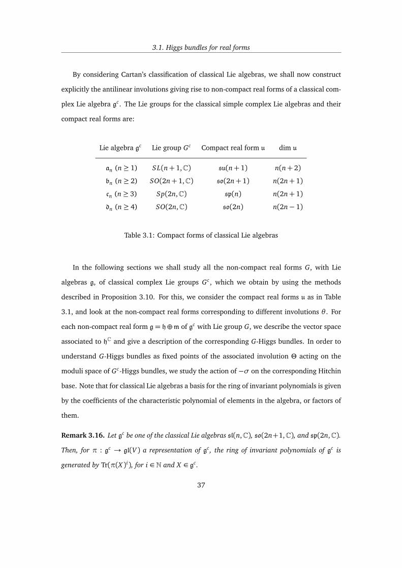
By considering Cartan’s classification of classical Lie algebras, we shall now construct
explicitly the antilinear involutions giving rise to non-compact real forms of a classical com-
plex Lie algebra gc . The Lie groups for the classical simple complex Lie algebras and their
compact real forms are:
Lie algebra gc Lie group Gc Compact real form u dim u
an (n≥ 1) SL(n+ 1,C) su(n+ 1) n(n+ 2)
bn (n≥ 2) SO(2n+ 1,C) so(2n+ 1) n(2n+ 1)
cn (n≥ 3) Sp(2n,C) sp(n) n(2n+ 1)
dn (n≥ 4) SO(2n,C) so(2n) n(2n− 1)
Table 3.1: Compact forms of classical Lie algebras
In the following sections we shall study all the non-compact real forms G, with Lie
algebras g, of classical complex Lie groups Gc , which we obtain by using the methods
described in Proposition 3.10. For this, we consider the compact real forms u as in Table
3.1, and look at the non-compact real forms corresponding to different involutions θ . For
each non-compact real form g= h⊕m of gc with Lie group G, we describe the vector space
associated to hC and give a description of the corresponding G-Higgs bundles. In order to
understand G-Higgs bundles as fixed points of the associated involution Θ acting on the
moduli space of Gc-Higgs bundles, we study the action of −σ on the corresponding Hitchin
base. Note that for classical Lie algebras a basis for the ring of invariant polynomials is given
by the coefficients of the characteristic polynomial of elements in the algebra, or factors of
them.
Remark 3.16. Let gc be one of the classical Lie algebras sl(n,C), so(2n+1,C), and sp(2n,C).
Then, for π : gc → gl(V ) a representation of gc , the ring of invariant polynomials of gc is
generated by Tr(π(X )i), for i ∈ N and X ∈ gc .
37
Chapter 3. Higgs bundles for non-compact real forms
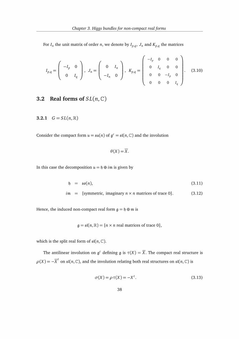
For In the unit matrix of order n, we denote by Ip,q, Jn and Kp,q the matrices
Ip,q =
−Ip 0
0 Iq
, Jn =
0 In
−In 0
, Kp,q =
−Ip 0 0 0
0 Iq 0 0
0 0 −Ip 0
0 0 0 Iq
. (3.10)
3.2 Real forms of SL(n,C)
3.2.1 G = SL(n,R)
Consider the compact form u= su(n) of gc = sl(n,C) and the involution
θ(X ) = X .
In this case the decomposition u= h⊕ im is given by
h = so(n), (3.11)
im = symmetric, imaginary n× n matrices of trace 0. (3.12)
Hence, the induced non-compact real form g= h⊕m is
g= sl(n,R) = n× n real matrices of trace 0,
which is the split real form of sl(n,C).
The antilinear involution on gc defining g is τ(X ) = X . The compact real structure is
ρ(X ) =−Xt
on sl(n,C), and the involution relating both real structures on sl(n,C) is
σ(X ) = ρτ(X ) =−X t . (3.13)
38

3.2. Real forms of SL(n,C)
Following Remark 3.14, we are interested in understanding the action of the involution Θ
induced from (3.13), acting on SL(n,C)-Higgs bundles (E,Φ).
Proposition 3.17. The involution σ induces the involution
Θ : (E,Φ) 7→ (E∗,Φt)
on the moduli space of SL(n,C) Higgs bundles. Thus, SL(n,R)-Higgs bundles are given by the
fixed points of Θ corresponding to automorphisms f : E→ E∗ giving a symmetric form on E.
Recalling that the trace is invariant under transposition, one has that the ring of invari-
ant polynomials of gc is acted on trivially by the involution −σ induced by (3.13).
3.2.2 G = SU∗(2m)
Consider the compact form u= su(2m) of gc = sl(n,C), for n= 2m, and let
θ(X ) = JmX J−1m ,
for
Jm =
0 Im
−Im 0
.
In this case, we have that u= h⊕ im for
h = sp(m), (3.14)
im =
Z1 Z2
Z2 −Z1
Z1 ∈ su(m), Z2 ∈ so(m,C)
. (3.15)
39

Chapter 3. Higgs bundles for non-compact real forms
The induced non-compact real form g= h⊕m is
g= su∗(2m) =
Z1 Z2
−Z2 Z1
Z1, Z2 m×m complex matrices,
TrZ1+ TrZ1 = 0
.
The antilinear involution on gc which fixes g is
τ(X ) = JmX J−1m . (3.16)
The compact real structure of sl(2m,C) is given by ρ(X ) =−Xt, and the involution relating
the compact structure and the non-compact structure τ is
σ(X ) =−JmX t J−1m . (3.17)
Proposition 3.18. The involution σ induces an involution
Θ : (E,Φ) 7→ (E∗,Φt)
on SL(2m,C) Higgs bundles. Since the maximal compact subgroup of SU∗(2m) is Sp(m), the
isomorphism classes of SU∗(2m)-Higgs bundles are given by fixed points of the involution Θ
corresponding to vector bundles E which have an automorphism f : E → E∗ endowing it with
a symplectic structure, and which trivialises its determinant bundle.
Concretely, SU∗(2m)-Higgs bundles are defined as follows:
Definition 3.19. An SU∗(2m) Higgs bundle on a compact Riemann surface Σ is given by
(E,Φ) for
E a rank 2m vector bundle with a symplectic form ω
Φ ∈ H0(Σ, End0(E)⊗ K) symmetric with respect to ω.
As the trace is invariant under conjugation and transposition, one has that the involu-
40

3.2. Real forms of SL(n,C)
tion −σ(X ) = JmX t J−1m induced from (3.17) acts trivially on the ring of invariant polyno-
mials of sl(2m,C).
3.2.3 G = SU(p, q)
Consider the compact form u= su(p+ q) of gc = sl(n,C), for p+ q = n, and the involution
θ(X ) = Ip,qX Ip,q,
where Ip,q is defined at (3.10). The compact form may be decomposed via the action of θ
as u= h⊕ im for
h =
a 0
0 b
a ∈ u(p), b ∈ u(q)
Tr(a+ b) = 0
, (3.18)
im =
0 Z
−Zt
0
Z p× q complex matrix
. (3.19)
The induced non-compact real form g= h⊕m is
su(p, q) =
Z1 Z2
Zt2 Z3
Z1, Z3 skew Hermitian of order p and q,
TrZ1+ TrZ3 = 0 , Z2 arbitrary
.
Considering the composition θρ on sl(p+q,C), for ρ the antilinear involution ρ(X ) =−X ∗,
we have that
θρ
Z1 Z2
Z3 Z4
= θ
−Zt1 −Z
t3
−Zt2 −Z
t4
=
−Zt1 Z
t3
Zt2 −Z
t4
.
41

Chapter 3. Higgs bundles for non-compact real forms
The fixed set of the antilinear involution θρ is precisely su(p, q) and hence the antilinear
involution on gc which fixes g is τ(X ) =−Ip,qXtIp,q. The compact real structure is given by
ρ(X ) =−Xt
on sl(n,C), and the involution relating both structures on sl(n,C) is
σ(X ) = Ip,qX Ip,q. (3.20)
Proposition 3.20. The involution σ on the Lie algebra induces an involution Θ on the moduli
space of SL(n,C)-Higgs bundles given by
(E,Φ) 7→ (E,−Φ).
Hence, SU(p, q) Higgs bundles are fixed points of the involution corresponding to bundles E
which have an automorphism conjugate to Ip,q sending Φ to −Φ, and whose ±1 eigenspaces
have dimensions p and q.
The centre of SU(p, q) is U(1), and its maximal compact subgroup is given by
H = S(U(p)× U(q)),
whose complexified Lie group is
HC = S(GL(p,C)× GL(q,C)) = (X , Y ) ∈ GL(p,C)× GL(q,C) : detY = (detX )−1.
By considering the Cartan involution on the complexified Lie algebra of SU(p, q) one has
su(p, q)C = sl(p+ q,C) = hC⊕mC,
where mC corresponds to the off diagonal elements of sl(p+ q,C). Hence, SU(p, q)-Higgs
bundles are defined as follows:
42
3.3. Real forms of SO(n,C)
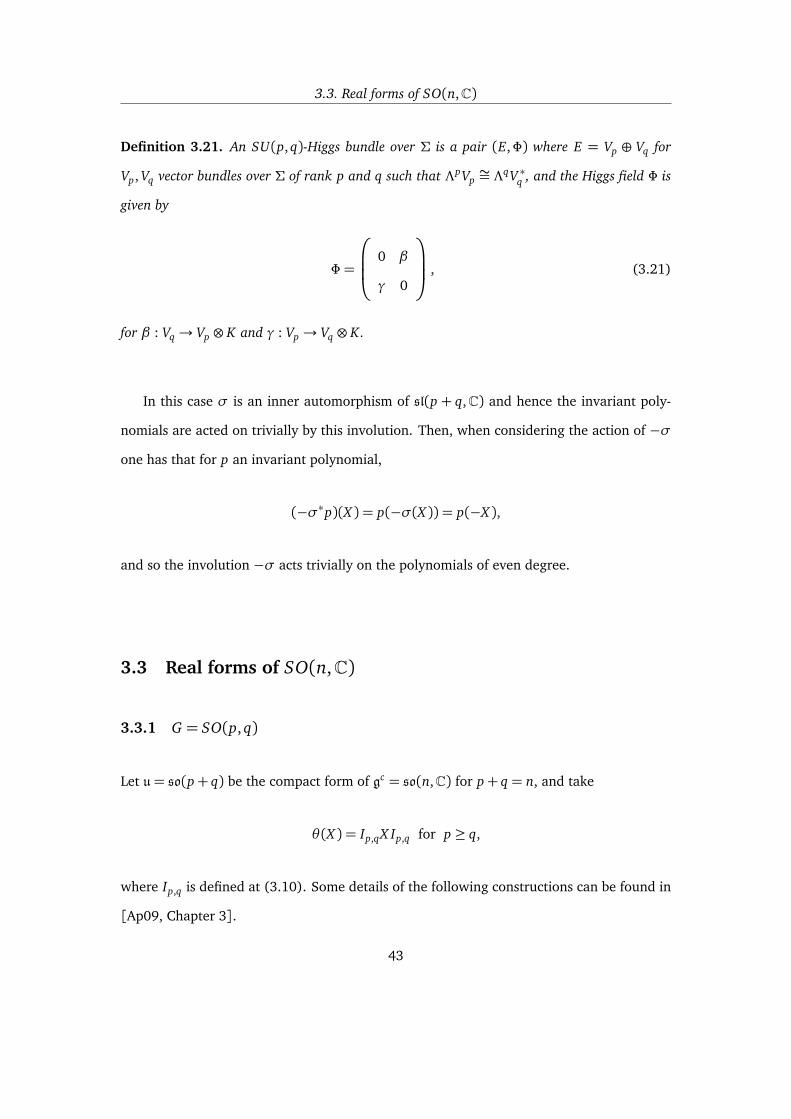
Definition 3.21. An SU(p, q)-Higgs bundle over Σ is a pair (E,Φ) where E = Vp ⊕ Vq for
Vp, Vq vector bundles over Σ of rank p and q such that ΛpVp∼= ΛqV ∗q , and the Higgs field Φ is
given by
Φ =
0 β
γ 0
, (3.21)
for β : Vq→ Vp ⊗ K and γ : Vp→ Vq ⊗ K.
In this case σ is an inner automorphism of sl(p + q,C) and hence the invariant poly-
nomials are acted on trivially by this involution. Then, when considering the action of −σ
one has that for p an invariant polynomial,
(−σ∗p)(X ) = p(−σ(X )) = p(−X ),
and so the involution −σ acts trivially on the polynomials of even degree.
3.3 Real forms of SO(n,C)
3.3.1 G = SO(p, q)
Let u= so(p+ q) be the compact form of gc = so(n,C) for p+ q = n, and take
θ(X ) = Ip,qX Ip,q for p ≥ q,
where Ip,q is defined at (3.10). Some details of the following constructions can be found in
[Ap09, Chapter 3].
43

Chapter 3. Higgs bundles for non-compact real forms
Considering the action of θ , the decomposition u= h⊕ im is given by
h =
X1 0
0 X3
X1 ∈ so(p), X3 ∈ so(q)
, (3.22)
im =
0 iX2
iX t2 0
X2 real p× q matrix
. (3.23)
The induced non-compact real form g= h⊕m of so(n,C) is
so(p, q) =
X1 X2
X t2 X3
All X i real , X2 arbitrary,
X1, X3 skew symmetric of order p and q
.
In this case, the parity of p+ q gives the following:
• if p+ q is even, g is a split real form if and only if p = q;
• if p+ q is odd, g is a split real form if and only if p = q+ 1.
The involution X 7→ Ip,qX Ip,q fixes the matrices in so(p+ q,C) of the form
X1 iX2
iX t2 X3
∼=
X1 X2
X t2 X3
,
where X i are all real, X2 is arbitrary and X1, X3 are skew symmetric.
The antilinear involution on gc which fixes g is τ(X ) = Ip,qX Ip,q. Note that the real struc-
ture τ commutes with the compact real structure ρ(X ) = X on gc , and thus the involution
relating both structures on gc is
σ(X ) = Ip,qX Ip,q. (3.24)
Proposition 3.22. The involution σ induces an involution Θ : (E,Φ) 7→ (E,−Φ) on the
44

3.3. Real forms of SO(n,C)
moduli space of SO(p + q,C) Higgs bundles. The SO(p, q) Higgs bundles are fixed points of
this involution corresponding to vector bundles E which have an automorphism f conjugate to
Ip,q sending Φ to −Φ and whose ±1 eigenspaces have dimensions p and q.
The vector space V associated to the standard representation of hC can be decomposed
into V = Vp ⊕ Vq, for Vp and Vq complex vector spaces of dimension p and q respectively,
with orthogonal structures. The maximal compact subalgebra of so(p, q) is h= so(p)×so(q)
and thus the Cartan decomposition of the complexification of so(p, q) is given by
so(p, q)C = so(p+ q,C) = (so(p,C)⊕ so(q,C))⊕mC,
where
m=
0 X2
X t2 0
X2 real p× q matrix
.
Definition 3.23. An SO(p, q) Higgs bundle is a pair (E,Φ) where E = Vp ⊕ Vq for Vp and Vq
complex vector spaces of dimension p and q respectively, with orthogonal structures, and the
Higgs field is a section in H0(Σ, (Hom(Vq, Vp)⊕Hom(Vp, Vq))⊗ K) given by
Φ =
0 β
γ 0
for γ≡−βT,
where βT is the orthogonal transpose of β .
Since the ring of invariant polynomials of gc = so(2m+ 1,C) is generated by Tr(X i) for
X ∈ gc , for p+ q = 2m+ 1 one has
(−σ∗p)(X ) = p(−σ(X )) = p(−X ) = p(X t) = p(X ).
Therefore, the involution −σ acts trivially on the ring of invariant polynomials of the Lie
45

Chapter 3. Higgs bundles for non-compact real forms
algebra so(2m+ 1,C), i.e., when p and q have different parity.
In the case of so(2m,C), for 2m= p+ q, the ring of invariant polynomials is generated
by Tr(X i) for X ∈ gc and i < 2m, together with the Pfaffian pm, which has degree m (e.g.
see [A89]). Note that when the automorphism f of E has determinant 1, i.e., when p and
q are even, the involution σ preserves orientation. Hence, if p ≡ q mod 4, one has
pm(−σ(X )) = σ∗pm(−X ) by definition
= pm(−X ) since σ preserves orientation
= pm(X ) since pm is of even degree.
(3.25)
Thus, the involution −σ acts trivially on the ring of invariant polynomials of so(2m,C)
when p and q are even and congruent mod 4. In particular, this is the case of the split real
form SO(p, p) for even p.
When p and q are odd, the involution σ is orientation reversing, and thus one has
pm(−σ(X )) = σ∗pm(−X ) by definition
= −pm(−X ) since σ reverses orientation
= pm(X ) if pm is of odd degree.
(3.26)
Hence, for p and q odd, −σ acts trivially on the ring of invariant polynomials of so(2m,C)
if p ≡ q mod 4.
3.3.2 G = SO∗(2m)
Let u= so(2m) be the compact form of so(n,C), for 2m= n, and consider the involution
θ(X ) = JmX J−1m ,
where Jm is given at (3.10).
46
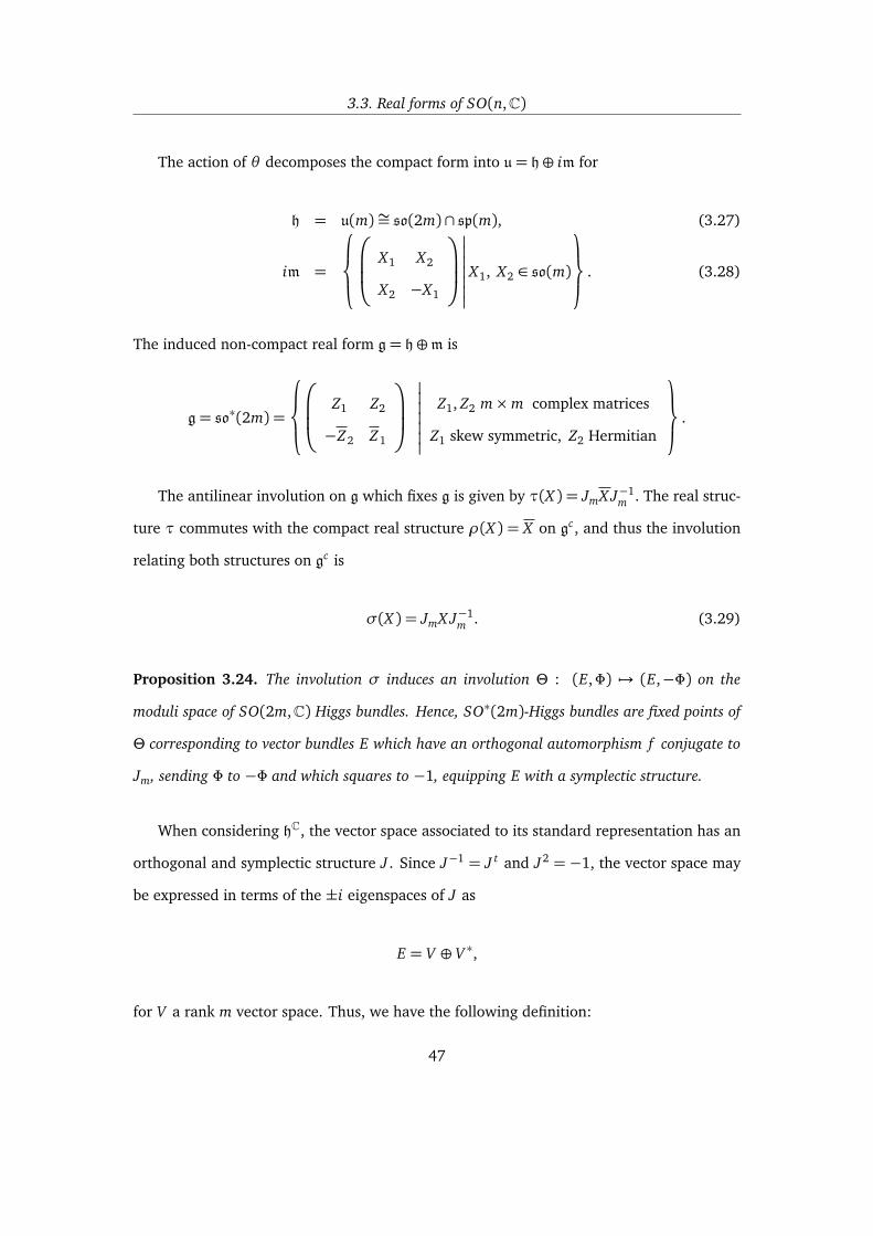
3.3. Real forms of SO(n,C)
The action of θ decomposes the compact form into u= h⊕ im for
h = u(m)∼= so(2m)∩ sp(m), (3.27)
im =
X1 X2
X2 −X1
X1, X2 ∈ so(m)
. (3.28)
The induced non-compact real form g= h⊕m is
g= so∗(2m) =
Z1 Z2
−Z2 Z1
Z1, Z2 m×m complex matrices
Z1 skew symmetric, Z2 Hermitian
.
The antilinear involution on g which fixes g is given by τ(X ) = JmX J−1m . The real struc-
ture τ commutes with the compact real structure ρ(X ) = X on gc , and thus the involution
relating both structures on gc is
σ(X ) = JmX J−1m . (3.29)
Proposition 3.24. The involution σ induces an involution Θ : (E,Φ) 7→ (E,−Φ) on the
moduli space of SO(2m,C) Higgs bundles. Hence, SO∗(2m)-Higgs bundles are fixed points of
Θ corresponding to vector bundles E which have an orthogonal automorphism f conjugate to
Jm, sending Φ to −Φ and which squares to −1, equipping E with a symplectic structure.
When considering hC, the vector space associated to its standard representation has an
orthogonal and symplectic structure J . Since J−1 = J t and J2 = −1, the vector space may
be expressed in terms of the ±i eigenspaces of J as
E = V ⊕ V ∗,
for V a rank m vector space. Thus, we have the following definition:
47
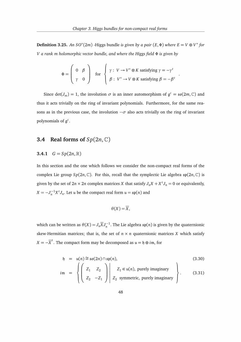
Chapter 3. Higgs bundles for non-compact real forms
Definition 3.25. An SO∗(2m) -Higgs bundle is given by a pair (E,Φ) where E = V ⊕ V ∗ for
V a rank m holomorphic vector bundle, and where the Higgs field Φ is given by
Φ =
0 β
γ 0
for
γ : V → V ∗⊗ K satisfying γ=−γt
β : V ∗→ V ⊗ K satisfying β =−β t.
Since det(Jm) = 1, the involution σ is an inner automorphism of gc = so(2m,C) and
thus it acts trivially on the ring of invariant polynomials. Furthermore, for the same rea-
sons as in the previous case, the involution −σ also acts trivially on the ring of invariant
polynomials of gc .
3.4 Real forms of Sp(2n,C)
3.4.1 G = Sp(2n,R)
In this section and the one which follows we consider the non-compact real forms of the
complex Lie group Sp(2n,C). For this, recall that the symplectic Lie algebra sp(2n,C) is
given by the set of 2n× 2n complex matrices X that satisfy JnX + X t Jn = 0 or equivalently,
X =−J−1n X t Jn. Let u be the compact real form u= sp(n) and
θ(X ) = X ,
which can be written as θ(X ) = JnX J−1n . The Lie algebra sp(n) is given by the quaternionic
skew-Hermitian matrices; that is, the set of n × n quaternionic matrices X which satisfy
X =−Xt. The compact form may be decomposed as u= h⊕ im, for
h = u(n)∼= so(2n)∩ sp(n), (3.30)
im =
Z1 Z2
Z2 −Z1
Z1 ∈ u(n), purely imaginary
Z2 symmetric, purely imaginary
. (3.31)
48

3.4. Real forms of Sp(2n,C)
The induced non-compact real form g= h⊕m is
g= sp(2n,R) =
X1 X2
X3 −X t1
X i real n× n matrices
X2, X3 symmetric
,
which is a split real form of gc .
The antilinear involution on sp(2n,C) which fixes g is given by τ(X ) = X , and the
compact real structure of gc is given by ρ(X ) = JnX J−1n . Hence, the involution relating
both real structures on gc is
σ(X ) = JnX J−1n . (3.32)
Proposition 3.26. The involution σ induces an involution
Θ : (E,Φ) 7→ (E,−Φ)
on the moduli space of Sp(2n,C) Higgs bundles. Hence, Sp(2n,R)-Higgs bundles are given by
the fixed points of Θ corresponding to vector bundles E which have a symplectic isomorphism
sending Φ to −Φ, and whose square is the identity, endowing E with an orthogonal structure.
As in the previous case, the 2n dimensional vector space associated to the standard
representation of hC has an orthogonal and a symplectic structure J , and hence it may be
expressed in terms of the ±i eigenspaces of J as E = V ⊕ V ∗.
Definition 3.27. An Sp(2n,R)-Higgs bundle is given by a pair (E,Φ) where E = V ⊕ V ∗ for
V a rank n holomorphic vector bundle, and for Φ the Higgs field given by
Φ =
0 β
γ 0
for
γ : V → V ∗⊗ K satisfying γ= γt
β : V ∗→ V ⊗ K satisfying β = β t.
49
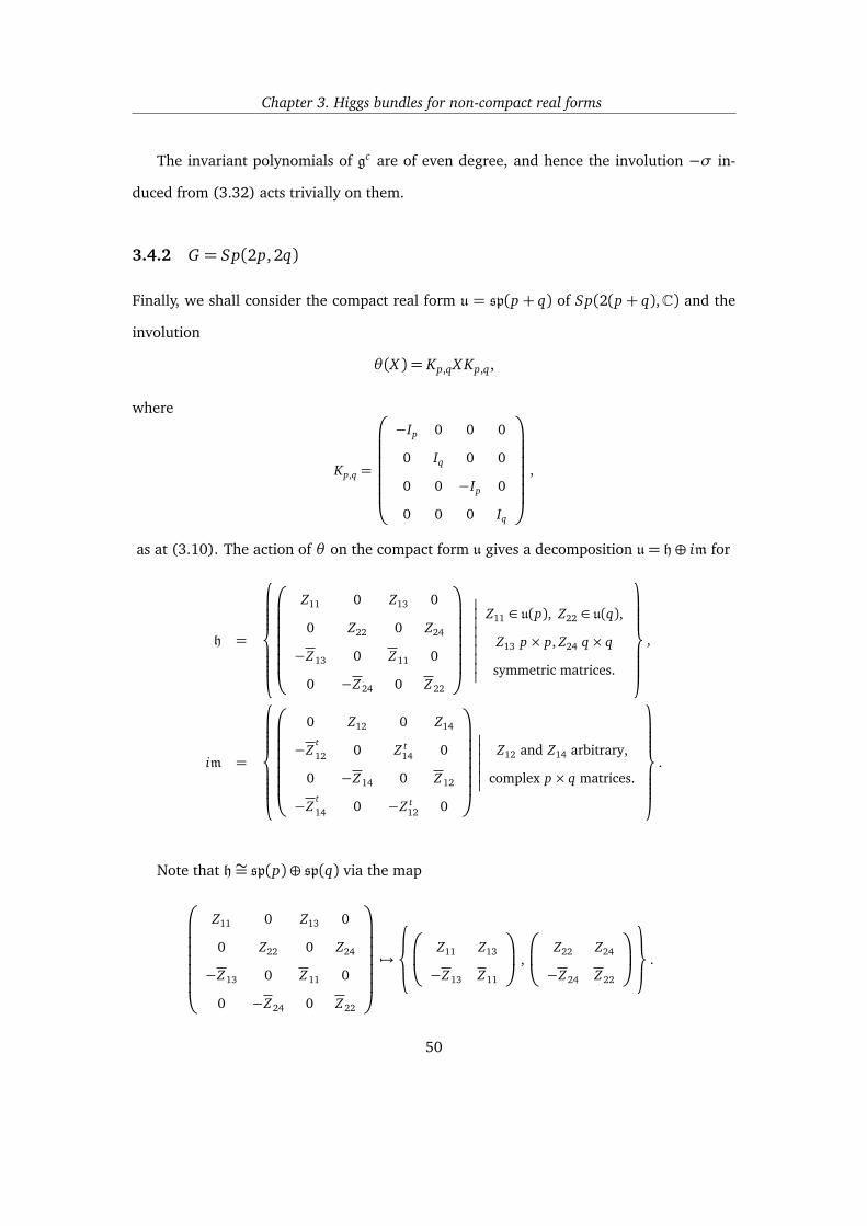
Chapter 3. Higgs bundles for non-compact real forms
The invariant polynomials of gc are of even degree, and hence the involution −σ in-
duced from (3.32) acts trivially on them.
3.4.2 G = Sp(2p, 2q)
Finally, we shall consider the compact real form u = sp(p + q) of Sp(2(p + q),C) and the
involution
θ(X ) = Kp,qX Kp,q,
where
Kp,q =
−Ip 0 0 0
0 Iq 0 0
0 0 −Ip 0
0 0 0 Iq
,
as at (3.10). The action of θ on the compact form u gives a decomposition u= h⊕ im for
h =
Z11 0 Z13 0
0 Z22 0 Z24
−Z13 0 Z11 0
0 −Z24 0 Z22
Z11 ∈ u(p), Z22 ∈ u(q),
Z13 p× p, Z24 q× q
symmetric matrices.
,
im =
0 Z12 0 Z14
−Zt12 0 Z t
14 0
0 −Z14 0 Z12
−Zt14 0 −Z t
12 0
Z12 and Z14 arbitrary,
complex p× q matrices.
.
Note that h∼= sp(p)⊕ sp(q) via the map
Z11 0 Z13 0
0 Z22 0 Z24
−Z13 0 Z11 0
0 −Z24 0 Z22
7→
Z11 Z13
−Z13 Z11
,
Z22 Z24
−Z24 Z22
.
50
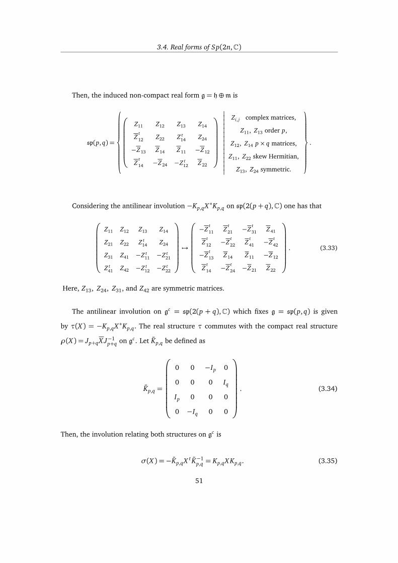
3.4. Real forms of Sp(2n,C)
Then, the induced non-compact real form g= h⊕m is
sp(p, q) =
Z11 Z12 Z13 Z14
Zt12 Z22 Z t
14 Z24
−Z13 Z14 Z11 −Z12
Zt14 −Z24 −Z t
12 Z22
Zi, j complex matrices,
Z11, Z13 order p,
Z12, Z14 p× q matrices,
Z11, Z22 skew Hermitian,
Z13, Z24 symmetric.
.
Considering the antilinear involution −Kp,qX ∗Kp,q on sp(2(p+ q),C) one has that
Z11 Z12 Z13 Z14
Z21 Z22 Z t14 Z24
Z31 Z41 −Z t11 −Z t
21
Z t41 Z42 −Z t
12 −Z t22
7→
−Zt11 Z
t21 −Z
t31 Z41
Zt12 −Z
t22 Z
t41 −Z
t42
−Zt13 Z14 Z11 −Z12
Zt14 −Z
t24 −Z21 Z22
. (3.33)
Here, Z13, Z24, Z31, and Z42 are symmetric matrices.
The antilinear involution on gc = sp(2(p + q),C) which fixes g = sp(p, q) is given
by τ(X ) = −Kp,qX ∗Kp,q. The real structure τ commutes with the compact real structure
ρ(X ) = Jp+qX J−1p+q on gc . Let Kp,q be defined as
Kp,q =
0 0 −Ip 0
0 0 0 Iq
Ip 0 0 0
0 −Iq 0 0
. (3.34)
Then, the involution relating both structures on gc is
σ(X ) =−Kp,qX t K−1p,q = Kp,qX Kp,q. (3.35)
51
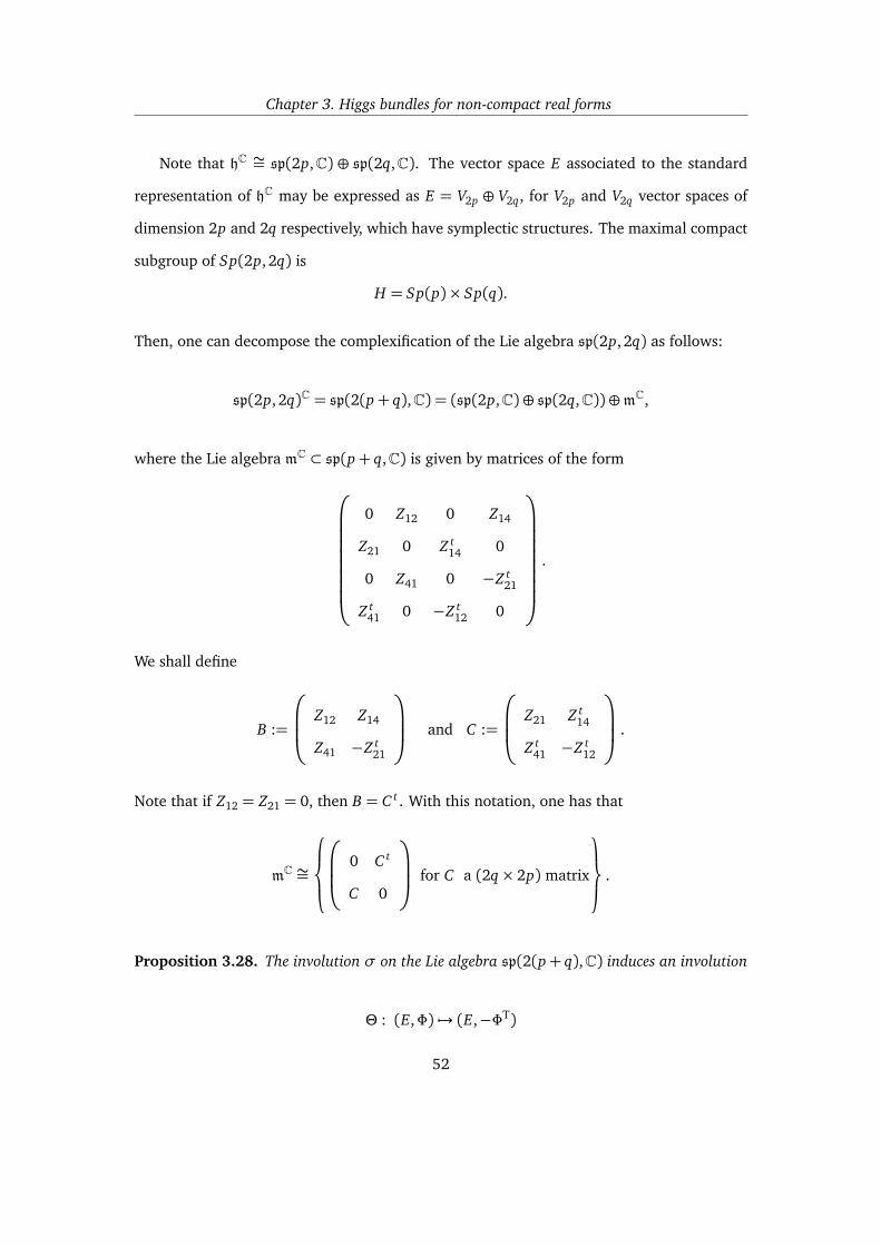
Chapter 3. Higgs bundles for non-compact real forms
Note that hC ∼= sp(2p,C) ⊕ sp(2q,C). The vector space E associated to the standard
representation of hC may be expressed as E = V2p ⊕ V2q, for V2p and V2q vector spaces of
dimension 2p and 2q respectively, which have symplectic structures. The maximal compact
subgroup of Sp(2p, 2q) is
H = Sp(p)× Sp(q).
Then, one can decompose the complexification of the Lie algebra sp(2p, 2q) as follows:
sp(2p, 2q)C = sp(2(p+ q),C) = (sp(2p,C)⊕ sp(2q,C))⊕mC,
where the Lie algebra mC ⊂ sp(p+ q,C) is given by matrices of the form
0 Z12 0 Z14
Z21 0 Z t14 0
0 Z41 0 −Z t21
Z t41 0 −Z t
12 0
.
We shall define
B :=
Z12 Z14
Z41 −Z t21
and C :=
Z21 Z t14
Z t41 −Z t
12
.
Note that if Z12 = Z21 = 0, then B = C t . With this notation, one has that
mC ∼=
0 C t
C 0
for C a (2q× 2p) matrix
.
Proposition 3.28. The involution σ on the Lie algebra sp(2(p+ q),C) induces an involution
Θ : (E,Φ) 7→ (E,−ΦT)
52

3.5. A geometric consequence
on the moduli space of Sp(2(p+q),C)-Higgs bundles. Hence, Sp(p, q)-Higgs bundles are given
by the fixed points of the involution Θ corresponding to symplectic vector bundles E which have
an endomorphism f : E→ E conjugate to Kp,q defined as at (3.34), sending Φ to the symplectic
transpose −ΦT, and whose ±1 eigenspaces are of dimension 2p and 2q.
Definition 3.29. An Sp(2p, 2q)-Higgs bundle is given by a pair (E,Φ) where E = V2p ⊕ V2q
is a direct sum of symplectic vector spaces of rank 2p and 2q, and where the symplectic Higgs
field is given by
Φ =
0 −γT
γ 0
for
γ : V2p→ V2q ⊗ K
−γT : V2q→ V2p ⊗ K,
for γT the symplectic transpose of γ.
The symplectic transpose of the map γ may be thought of as follows. Since V and
W are symplectic vector bundles, there are two induced isomorphisms qV : V ∗ → V and
qW : W →W ∗. Via these isomorphisms, we define γT = qVγtqW , where γt is the dual action
of γ.
As the trace is invariant under conjugation and transposition, the involution −σ in-
duced from (3.35) acts trivially on the ring of invariant polynomials of the Lie algebra
gc = sp(2(p+ q),C).
3.5 A geometric consequence
Having studied the action of the different involutions −σ on the ring of invariant polyno-
mials of each complex simple lie algebra gc , we have the following.
Proposition 3.30. For each non-compact real form of gc = so(2m+1,C) and gc = sp(2n,C),
the corresponding involution −σ acts trivially on the ring of invariant polynomials of gc .
53
Chapter 3. Higgs bundles for non-compact real forms
Hence, for Gc = Sp(2n,C) and SO(2m+ 1,C), the induced involutions
Θ : (E,Φ) 7→ (σ(E),−σ(Φ))
on the moduli spaces MGc preserve each fibre of the Hitchin fibration. In the case of
SO(2m,C) one has two different situations:
Proposition 3.31. For gc = so(2m,C), the action of the different involutions −σ is given as
follows:
• the involution −σ associated to SO∗(2m) acts trivially on the ring of invariant polyno-
mials of gc;
• the involution −σ induced by SO(p, q) for p and q both even, or both odd, acts trivially
on the invariant polynomials of so(2m,C) if p ≡ q mod 4. Otherwise, it acts trivially on
the basic polynomials except for the Pfaffian.
From Proposition 3.31, each fibre of the SO(2m,C) Hitchin fibration is preserved by the
involution Θ defining the real form SO∗(2m), and by the involution defining the real form
SO(p, q) only if p ≡ q mod 4.
Proposition 3.32. Consider gc = sl(n,C). Then,
• the involution −σ associated to the non-compact real forms sl(n,R) and su∗(2m), when
n= 2m, acts trivially on the ring of invariant polynomials of gc;
• the involution −σ associated to the non-compact real form su(p, q) of sl(p+ q,C) acts
trivially only on the invariant polynomials of even degree.
From Proposition 3.32, the involution −σ induces Θ : (P,Φ) 7→ (σ(P),−σ(Φ)) on
the moduli space of SL(n,C)-Higgs bundles, which preserve each fibre of the SL(n,C)
Hitchin fibration except when σ corresponds to the real form SU(p, q). In this case, Θ only
preserves the fibres over differentials of even degree.
54
Chapter 4
Higgs bundles for split real forms
As mentioned in Chapter 3, in [Hit92] Hitchin gives an explicit description of a component
of the space of representations of π1(Σ) into split real forms in terms of Higgs bundles. In
this chapter we shall consider this component to study the space of Higgs bundles for split
real forms.
We begin by introducing three dimensional subalgebras as defined by Kostant (see
[Kos59], [Kos63]), and follow the steps in [Hit92] to define an involution σs on a complex
Lie algebra which is closely related to its split real form, and which coincides in the case of
classical groups with the involution σ associated to split real forms as defined in Chapter
3. By means of the involution in the Lie theoretic setting, in Section 4.2, we study the fixed
points of the induced involution Θ on the Hitchin fibration for the corresponding complex
Lie group.
4.1 An algebraic approach
In this section we set up the Lie theoretic background needed to study Higgs bundles for
split real forms. We shall denote by gc a complex simple Lie algebra of rank r.
55

Chapter 4. Higgs bundles for split real forms
4.1.1 Three dimensional subalgebras
From [Kos59] we consider the following subalgebra of a complex simple Lie algebra gc (see
also details in [Hit92, Section 4]):
Definition 4.1. A three-dimensional subalgebra s of gc is a subalgebra of gc generated by a
semisimple element h0, and nilpotent elements e0 and f0 of gc satisfying the relations
[h0, e0] = e0 ; [h0, f0] =− f0 ; [e0, f0] = h0. (4.1)
By the Jacobson-Morosov lemma (see [J51] and [Mor42]), any nilpotent element of gc
can be embedded into a three dimensional subalgebra whose generators satisfy (4.1), i.e.,
a copy of sl(2,C) in gc . A nilpotent element e0 ∈ gc is called principal if its centralizer is r-
dimensional. When the nilpotent elements of a three-dimensional subalgebra are principal,
the subalgebra is called a principal three dimensional subalgebra. Any complex simple Lie
algebra gc has a unique (up to conjugacy) principal three dimensional subalgebra [Kos59,
Section 5].
Following [Kos59, Section 5], one may construct a principal three dimensional subal-
gebra of a complex simple Lie algebra gc as follows. Consider h a Cartan subalgebra of gc ,
and denote by ∆ the root system. For α ∈ ∆, we let xα be the root vectors satisfying the
standard relation
[xα, x−α] = α.
We write ∆+ for a system of positive roots and define Π = α1,α2, . . . ,αr the correspond-
ing simple roots. Let hαi, eα, e−α be a fixed basis, for α ∈ ∆+ and αi ∈ Π, and h0 the
element defined by
h0 :=1
2
r∑
i=1
hαi. (4.2)
56

4.1. An algebraic approach
Then, h0 may be expressed as
h0 =r∑
i=1
riαi
for some positive half integers ri . By considering the numbers ri , we further define f0 and
e0 as follows:
e0 :=r∑
i=1
cieαi, (4.3)
f0 :=r∑
i=1
(ri/ci)e−αi, (4.4)
where ciri=1 are any non-zero complex numbers. The subalgebra generated by h0, e0, f0
is a principal three dimensional subalgebra.
Given a root λ ∈∆, the order o(λ) of λ is the integer
o(λ) =∑
α∈Πnα, (4.5)
where nα ∈ N are uniquely defined by
λ=∑
α∈Πnαα.
Let ψ be the highest root. Then, we may write
ψ=r∑
i=1
qiαi .
Remark 4.2. Considering e0 and f0 as defined as in (4.3) and (4.4), for ci :=pqi and ri = qi ,
the subalgebra
s0 =<ψ, e0, f0 > (4.6)
is a principal three dimensional subalgebra of gc .
57
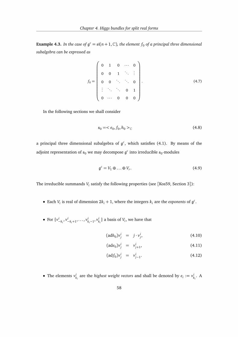
Chapter 4. Higgs bundles for split real forms
Example 4.3. In the case of gc = sl(n+1,C), the element f0 of a principal three dimensional
subalgebra can be expressed as
f0 =
0 1 0 · · · 0
0 0 1. . .
...
0 0. . .
. . . 0...
. . .. . . 0 1
0 · · · 0 0 0
. (4.7)
In the following sections we shall consider
s0 =< e0, f0, h0 >C (4.8)
a principal three dimensional subalgebra of gc , which satisfies (4.1). By means of the
adjoint representation of s0 we may decompose gc into irreducible s0-modules
gc = V1⊕ . . .⊕ Vr . (4.9)
The irreducible summands Vi satisfy the following properties (see [Kos59, Section 3]):
• Each Vi is real of dimension 2ki + 1, where the integers ki are the exponents of gc .
• For v i−ki
, v i−ki+1, . . . , v i
ki−1, v iki a basis of Vi , we have that
(adh0)vij = j · v i
j , (4.10)
(ade0)vij = v i
j+1, (4.11)
(ad f0)vij = v i
j−1. (4.12)
• The elements v iki
are the highest weight vectors and shall be denoted by ei := v iki
. A
58
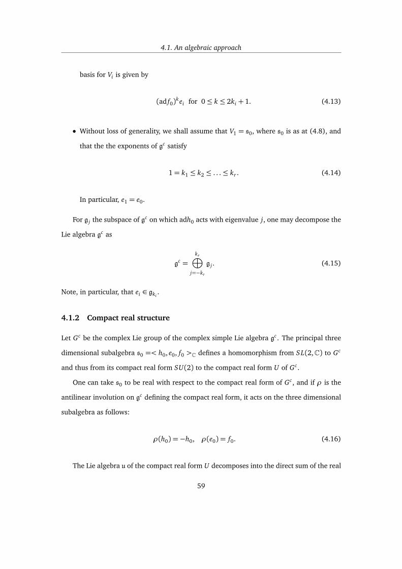
4.1. An algebraic approach
basis for Vi is given by
(ad f0)kei for 0≤ k ≤ 2ki + 1. (4.13)
• Without loss of generality, we shall assume that V1 = s0, where s0 is as at (4.8), and
that the the exponents of gc satisfy
1= k1 ≤ k2 ≤ . . .≤ kr . (4.14)
In particular, e1 = e0.
For g j the subspace of gc on which adh0 acts with eigenvalue j, one may decompose the
Lie algebra gc as
gc =kr⊕
j=−kr
g j . (4.15)
Note, in particular, that ei ∈ gki.
4.1.2 Compact real structure
Let Gc be the complex Lie group of the complex simple Lie algebra gc . The principal three
dimensional subalgebra s0 =< h0, e0, f0 >C defines a homomorphism from SL(2,C) to Gc
and thus from its compact real form SU(2) to the compact real form U of Gc .
One can take s0 to be real with respect to the compact real form of Gc , and if ρ is the
antilinear involution on gc defining the compact real form, it acts on the three dimensional
subalgebra as follows:
ρ(h0) =−h0, ρ(e0) = f0. (4.16)
The Lie algebra u of the compact real form U decomposes into the direct sum of the real
59

Chapter 4. Higgs bundles for split real forms
representations, which by abuse of notation we denote V1, . . . , Vr . In particular, (4.9) is the
complexification of
u=r⊕
i=1
Vi .
4.1.3 A natural involution on Lie algebras
As before, consider gc a complex simple Lie algebra of rank r, and let s0 =< h0, e0, f0 >
be a principal three dimensional subalgebra as defined at (4.8) in Section 4.1. Denote by
e1, . . . , er the highest weight vectors of the irreducible representations Vi . Following [Hit92,
Proposition 6.1] we define the following involution.
Definition 4.4. There is a natural involution σs on the Lie algebra gc given by
σs([ad f0]nei) = (−1)n+1[ad f0]
nei . (4.17)
This involution is a Lie algebra automorphism and is uniquely defined by
σs(ei) =−ei and σs( f0) =− f0.
Note that as e1 = e0 we have that (ad f0)e1 = h0 and hence σs(h0) = h0. The fixed
points of σs are described as follows:
Proposition 4.5 ([Hit92]). Let gc be a complex simple Lie algebra with principal three dimen-
sional subalgebra s0 =< h0, e0, f0 >C, and ei the corresponding highest weight vectors. Then,
the fixed point set of the involution σs defined in (4.4) is the complexification of a maximal
compact subalgebra of the split real form g of gc , as defined in Definition 3.6.
Proof. For completeness, we sketch here the proof given in [Hit92, Section 6] of this propo-
sition, and refer to interesting results from [Kos59]. Let us consider the usual compact real
60
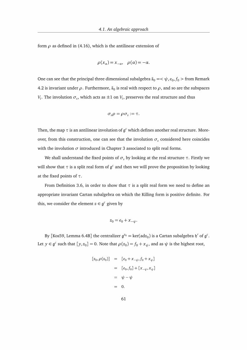
4.1. An algebraic approach
form ρ as defined in (4.16), which is the antilinear extension of
ρ(xα) = x−α, ρ(α) =−α.
One can see that the principal three dimensional subalgebra s0 =<ψ, e0, f0 > from Remark
4.2 is invariant under ρ. Furthermore, s0 is real with respect to ρ, and so are the subspaces
Vi . The involution σs, which acts as ±1 on Vi , preserves the real structure and thus
σsρ = ρσs := τ.
Then, the map τ is an antilinear involution of gc which defines another real structure. More-
over, from this construction, one can see that the involution σs considered here coincides
with the involution σ introduced in Chapter 3 associated to split real forms.
We shall understand the fixed points of σs by looking at the real structure τ. Firstly we
will show that τ is a split real form of gc and then we will prove the proposition by looking
at the fixed points of τ.
From Definition 3.6, in order to show that τ is a split real form we need to define an
appropriate invariant Cartan subalgebra on which the Killing form is positive definite. For
this, we consider the element z ∈ gc given by
z0 = e0+ x−ψ.
By [Kos59, Lemma 6.4B] the centralizer gz0 = ker(adz0) is a Cartan subalgebra h′ of gc .
Let y ∈ gc such that [y, z0] = 0. Note that ρ(z0) = f0+ xψ, and as ψ is the highest root,
[z0,ρ(z0)] = [e0 + x−ψ, f0 + xψ]
= [e0, f0] + [x−ψ, xψ]
= ψ−ψ
= 0.
61
Chapter 4. Higgs bundles for split real forms
Then, h′ is also the centralizer of ρ(z0) and thus is preserved by the compact real structure
ρ. For y ∈ h′ one has [z0, y] = 0. Recalling that ψ is the highest root, one can show that
y = u+ v,
where u commutes with e0 and v commutes with f0. By definition, the involution σs acts
as −1 on the centralizer of e0 and f0, and hence acts as −1 on h′. The Cartan subalgebra h′
is preserved by τ, and for y ∈ h′ fixed by ρ we have that
τ(i y) = σsρ(i y) = σs(−i y) = i y.
Recall that the Killing form restricted to the compact real form ρ is negative definite. Hence,
on the fixed points of τ, the Killing form is positive definite and thus the real form τ is a
split real form.
Finally, in order to understand the fixed point set of σs, we shall treat gc as a real Lie
algebra, and decompose it into the eigenspaces of σs and ρ:
gc = g++⊕ g+−⊕ g−+⊕ g−−, (4.18)
where the lower index gives the sign of the σs-eigenvalue, and the upper index gives the
sign of the ρ-eigenvalue. With this notation, the fixed point set of σs is
gσs = g++⊕ g−+, (4.19)
and the fixed point set of τ= ρσs is
g= g++⊕ g−−. (4.20)
By definition the Killing form is negative definite on g−− and positive definite on g++. Hence,
62

4.1. An algebraic approach
g++ is the maximal compact subalgebra of g. Furthermore, g++ is a compact form of gσs
defined by the restriction of ρ to the fixed point set of σs. Then, the complex Lie algebra
gσs can be seen as the complexification of the maximal compact subalgebra g++ of the split
real form gr as required.
Remark 4.6. Note that in the case of classical Lie algebras, the involution σs considered in
Proposition 4.5 corresponds to the involution σ introduced in Chapter 3 for the non-compact
real forms sl(n,R), so(p, p), so(p, p+ 1) and sp(2n,R).
In the proof of Proposition 4.5 we considered the decomposition
gc = g++⊕ g+−⊕ g−+⊕ g−−,
where the upper index corresponds to the±1 eigenspace of the compact antilinear-involution
of gc , and the lower index corresponds to the ±1 eigenspace of σs. With this notation, the
compact real form u considered in Chapter 3 is given by
u = g++⊕ g+−, (4.21)
In particular, ig++ = g−+ and ig+− = g−−.
4.1.4 The Kostant slice
The highest weight vectors ei of Vi introduced in (4.13) generate the following affine sub-
space of gc:
Definition 4.7. We call the Kostant slice K of gc the space given by
K := f ∈ gc | f = f0+ a1e1+ a2e2+ . . .+ ar er, (4.22)
for ei the highest weight vectors of gc and ai complex numbers, and f0 as at Definition 4.1.
63
Chapter 4. Higgs bundles for split real forms
Remark 4.8. Note that by Definition 4.4, the involution σs acts as −1 on elements in the
Kostant slice, and hence the involution −σs preserves K .
Denote by G the ring of invariant polynomials in gc and let
p1, . . . , pr, (4.23)
be a choice of a homogeneous basis for this ring, where deg(p1) ≤ . . . ≤ deg(pr). From
[Ca50] and [Ch50], we may choose the basis such that deg(pi) = ki + 1, and from [Kos63,
Theorem 7] the choice can be done such that if f ∈K , then pi( f ) = ai . For f ∈ gc , denote
by g f the orbits of f of the adjoint action of G on gc . The set
D =⋃
f ∈K
g f
is a dense set in gc .
Proposition 4.9. The involution −σs on gc induced from Definition 4.4 acts trivially on the
ring of invariant polynomials of gc .
Proof. Let us consider the basis p1, . . . , pr of invariant polynomials as defined previously.
As the basis of invariant polynomials is invariant under conjugation, we have that for f ∈K
and X ∈ g f , the involution σs acts as follows:
(−σ∗s pi)(X ) = (−σ∗s )pi( f ) since X ∈ g f
= pi(−σs( f )) by definition of σs
= pi( f ) by Remark 4.8, since f ∈K
= pi(X ) since X ∈ g f .
As these equalities hold for any X , by continuity the ring of invariant polynomials is acted
on trivially by −σs.
64

4.2. The Hitchin fibration
Remark 4.10. Note that Proposition 4.9 agrees with Section 3.5, since the involution σs as
defined in Definition 4.4 corresponds to the involution σ associated to the split real forms of
sl(n,C), so(n,C) and sp(2n,C).
4.2 The Hitchin fibration
As seen in Chapter 3, the involution σs associated to a split real form g of gc induces an
involution on the moduli spaceMGc of Gc-Higgs bundles, whose action on a Higgs bundle
(E,Φ) is given by
Θ : (E,Φ) 7→ (σs(E),−σs(Φ)).
By means of the explicit description of σs given in the previous section, we shall give
an interpretation of Proposition 4.9 from the point of view of Higgs bundles.
4.2.1 The Teichmüller component
We shall describe here the construction of the Teichmüller component following [Hit92].
Consider the adjoint group AdGc of a complex simple Lie group Gc , and P a principal AdGc-
bundle. We let gc be the corresponding complex simple Lie algebra, and s0 =< h0, e0, f0 >C
be its principal three dimensional subalgebra as at (4.8).
Recall that forMAdGc the moduli space of AdGc-Higgs bundles, the Hitchin fibration is
given by the proper map
h :MAdGc → AAdGc :=⊕
H0(Σ, Kki+1) (4.24)
(E,Φ) 7→ (p1(Φ), p2(Φ), . . . , pr(Φ)), (4.25)
where p1, . . . , pr is a basis of invariant polynomials on gc as defined in (4.23). The Teich-
müller component [Hit92] is induced by the Kostant slice introduced in Definition 4.7, and
is constructed as follows. From the decomposition of gc into eigenspaces of adh0, consider
65

Chapter 4. Higgs bundles for split real forms
the vector bundle
E = adP ⊗C=kr⊕
j=−kr
g j ⊗ K j , (4.26)
where kr =maxkii is the maximal exponent of gc (see (4.14)). This is the adjoint bundle
of gc associated to the principal AdGc-bundle P = P1 ×i G, where P1 is the holomorphic
principal SL(2,C)-bundle associated to K−1/2⊕K1/2, and i : SL(2,C) ,→ AdGc is the inclu-
sion corresponding to the principal three dimensional subalgebra s0. Although P1 involves
a choice of square root K1/2, the bundle E is independent of it. The AdGc-Higgs bundle
(E,Φ), for
Φ = f0+ a1e1+ a2e2+ . . .+ ar er (4.27)
and ai ∈ H0(Σ, Kki+1), is stable. Note that (adh0) f0 = − f0 and thus we may regard f0 as
a section of (g−1 ⊗ K−1)⊗ K . Furthermore, the highest weight vectors e j ∈ gk jand thus
a je j is a section of gk j⊗ Kk j+1, making Φ a well defined holomorphic section of E ⊗ K .
As pi(Φ) = ai , the above construction defines a section s : (a1, . . . , ar) 7→ (E,Φ) of MAdGc
whose image is the Teichmüller component. This component defines an origin in the smooth
fibres of h, and thus one has a fibration of abelian varieties.
4.2.2 Principal Higgs bundles and split real forms
The natural involution σs on E = adP⊗C given in Definition 4.4 acts on Higgs fields of the
form of (4.27) as σs(Φ) = −Φ. Hence, the involution −σs fixes these Higgs bundles, and
thus preserves the Teichmüller component. From Chapter 3, the involution σs induces an
involution Θ onMAdGc which acts as
Θ : (E,Φ) 7→ (σs(E),−σs(Φ)).
66

4.2. The Hitchin fibration
The fixed point sets inMAdGc of the involution Θ correspond to the moduli space of reduc-
tive representations of π1(Σ) into the split real form of AdGc . The following result ([Hit92,
Theorem 7.5]) relates the Teichmüller component to the space of representations of the
split real form of AdGc:
Theorem 4.11. The section s ofMAdGc defines a smooth connected component of the moduli
space of reductive representations of π1(Σ) into the split real form of AdGc .
From Proposition 4.9 the involution −σs acts trivially on the ring of invariant polyno-
mials on gc , and thus Θ preserves each fibre of the Hitchin fibration. In order to study
the fixed point set of Θ, we note that the involution Θ acts trivially on the Teichmüller
component of MAdGc . As mentioned before, by choosing a square root K1/2, we obtain a
choice of Teichmüller component which makes the fibres be abelian varieties. Moreover,
since Gc gives a covering of AdGc , when considering the moduli spaceMGc , there could be
more than one lift of the Teichmüller component depending on whether the maximal three
dimensional subgroup is SL(2,R) or SO(3). Thus, by choosing one of these components
we obtain an origin in the fibres of the Hitchin fibrationMGc →AGc .
Recall that the fixed point sets of Θ induced by σs give the subspace of Higgs bundles
corresponding to the split real form of Gc . The reader should refer to [Hit92, Theorem 10.2]
for an example of the analysis of the Teichmüller components in the case of PSL(n,R).
Theorem 4.12. The intersection of the subspace of the Higgs bundle moduli spaceMGc corre-
sponding to the split real form of gc with the smooth fibres of the Hitchin fibration
h : MGc →AGc ,
is given by the elements of order two in those fibres.
Proof. An infinitesimal deformation of a Higgs bundle (E,Φ) is given by (A, Φ), where
A ∈ Ω01(End0E) and Φ ∈ Ω10(End0E). The holomorphic involution Θ on MGc induces
67
Chapter 4. Higgs bundles for split real forms
an involution on the tangent space T of MGc at a fixed point of Θ. Moreover, as seen in
(3.1) there is a natural symplectic form ω defined on the infinitesimal deformations by
ω((A1, Φ1), (A2, Φ2)) =
∫
Σtr(A1Φ2− A2Φ1). (4.28)
As the trace is invariant under Θ and σs(Φi) = −Φi , the induced involution on the tangent
space maps ω 7→ −ω. It follows that the ±1-eigenspaces T± of this involution are isotropic
and complementary, and hence Lagrangian. Let us denote by Dh the derivative of
h :MGc →AGc ,
which maps the tangent spaces ofMGc to the tangent space of the base AGc . As the map
h is invariant under the involution Θ, the eigenspace T− is contained in the kernel of Dh.
Since the derivative is surjective at a regular point, its kernel has dimension dim(M )/2
and thus it equals T−. Then, Dh is an isomorphism from T+ to the tangent space of the
base. Since h is a proper submersion on the fixed point set, it defines a covering space.
The tangent space to the identity in the fibres is acted as −1 by the involution Θ and as
the fibres are connected [DoPa12], by exponentiation, the action of Θ on the regular fibres
corresponds to x 7→ −x . Hence, the points of order two in the fibresMreg ofMGc over the
regular locus Areg correspond to Higgs bundles for the associated split real form, i.e., to
fixed points of Θ.
For σs a Lie algebra involution associated to the split real form of a complex Lie group
Gc , the fixed points of the involution Θ : (E,Φ) 7→ (σs(E),−σs(Φ)) onMGc give a covering
of the regular locus of Areg . Such a covering is defined by the action of π1(Areg), giving
a permutation on the fibres. In the case of the split real form SL(n,R) of SL(n,C), the
fixed points of Θ in MSL(n,C) are given by points of order two in the Prym varieties. In
the following chapter we shall study the particular case of SL(2,R)-Higgs bundles via the
action of π1(A ).
68

Chapter 5
Monodromy of the SL(2,R) Hitchin
fibration Hitchin fibration
In Chapter 4 we gave a description of Higgs bundles associated to a split real form G of a
complex simple Lie group Gc in terms of the points of order two in the regular fibres of the
Hitchin fibration of Gc-Higgs bundles. It is thus natural to consider the monodromy action
in order to study the moduli space of G-Higgs bundles for a split real form.
In this Chapter we shall focus on the split real form SL(2,R) of SL(2,C), and the
associated Higgs bundles. For this in Section 5.1 we introduce the Hitchin fibration for
SL(2,C)-Higgs bundles, expanding the descriptions given in Chapter 3. Then, in Section 5.2
we define the holonomy homomorphism and review Copeland’s analysis of the monodromy
action [Cop05]. Finally, in Section 5.3 we give an explicit description of the monodromy
action for the SL(2,R) Hitchin fibration. The results from this Chapter have been accepted
for publication in [Sch11], and an application of them is given in Chapter 8.
69
Chapter 5. Monodromy of the SL(2,R) Hitchin fibration Hitchin fibration
5.1 The SL(2,C) Hitchin fibration
We begin by describing the Hitchin fibration for SL(2,C), and then introduce the work of
Copeland [Cop05], in which the monodromy of the Hitchin fibration is analysed from a
graph theoretic point of view.
As in previous chapters, let Σ be a Riemann surface of genus g ≥ 3, and let K be its
canonical bundle. We have seen in Chapter 3 that an SL(2,C)-Higgs bundle as defined by
Hitchin [Hit87] and Simpson [S92] is given by a pair (E,Φ), where E is a rank 2 holomor-
phic vector bundle with det(E) = OΣ and the Higgs field Φ is a section of End0(E) ⊗ K ,
where End0(E) denotes the bundle of traceless endomorphisms of E.
For simplicity, we shall drop the subscript of MSL(2,C) and denote by M the moduli
space of S-equivalence classes of semistable SL(2,C)-Higgs bundles. Considering the map
Φ 7→ det(Φ), one has the Hitchin fibration [Hit87]
h :M → A := H0(Σ, K2),
where A is the Hitchin base, introduced in Chapter 2 as ASL(2,C). The moduli spaceM is
homeomorphic to the moduli space of reductive representations of the fundamental group
of Σ in SL(2,C) via non-abelian Hodge theory [Cor88], [D87], [Hit87], [S92].
5.1.1 The regular fibres of the Hitchin fibration
From [Hit87, Theorem 8.1] the Hitchin map h is proper and surjective, and its regular
fibres are abelian varieties. Moreover, for any a ∈ A − 0 the fibre Ma is connected
[GO12, Theorem 8.1]. For any isomorphism class of (E,Φ) in M , one may consider the
zero set of its characteristic polynomial
det(Φ−ηI) = η2+ a = 0,
70
5.1. The SL(2,C) Hitchin fibration
where a = det(Φ) ∈ A . This defines a spectral curve ρ : S → Σ in the total space X on
K , for η the tautological section of the pull back of K on X . We shall denote byMreg the
regular fibres of the Hitchin map h, and let Areg be the regular locus of the base, which
is given by quadratic differentials with simple zeros. Note that the curve S is non-singular
over the regular locus Areg , and the ramification points are given by the intersection of S
with the zero section. The curve S has a natural involution τ(η) = −η and thus we can
define the Prym variety Prym(S,Σ) as the set of line bundles M ∈ Jac(S) which satisfy
τ∗M ∼= M∗.
In particular, this definition is consistent with the one given in Chapter 2 by means of the
Norm map. Furthermore, as seen in Chapter 2, from [Hit87, Theorem 8.1] the regular
fibres ofM are isomorphic to Prym(S,Σ).
5.1.2 The involution Θ
Recall from Proposition 3.17 that the involution on SL(2,C) corresponding to the real form
SL(2,R) defines an antiholomorphic involution on the moduli space of representations
which, in the Higgs bundle complex structure, is the holomorphic involution
Θ : (E,Φ) 7→ (E,−Φ),
whose associated automorphism f : E → E∗ gives a symmetric form on E. In particular,
the isomorphism classes of stable Higgs bundles with Φ 6= 0 fixed by the involution Θ
correspond to SL(2,R)-Higgs bundles (E = V ⊕ V ∗,Φ), where V is a line bundle on Σ, and
the Higgs field Φ is given by
Φ =
0 β
γ 0
,
71

Chapter 5. Monodromy of the SL(2,R) Hitchin fibration Hitchin fibration
for β : V ∗ → V ⊗ K and γ : V → V ∗ ⊗ K . As mentioned in Example 3.13, the isomorphism
class of an SL(2,C)-Higgs bundle with Φ = 0 corresponds to the compact real form.
From [Hit87], the smooth fibres are tori of real dimension 6g − 6. Indeed, the Higgs
bundles in Example 2.7 give a section of the fibration fixed by Θ, which defines the Teich-
müller component introduced in Chapter 4, and this allows us to identify each fibre with
an abelian variety, in fact, a Prym variety as described in Chapter 2. Since the involution Θ
leaves invariant det(Φ), it defines an involution on each fibre of the Hitchin fibration.
As shown in Chapter 4, the fixed points of the involution Θ on the regular fibres of
the Hitchin fibration h : M → A are the elements of order 2 in the abelian varieties.
Hence, the points corresponding to SL(2,R)-Higgs bundles give a covering space of Areg .
Since a generic fibre of h is given by the abelian variety Prym(S,Σ), i.e., by the quotient
of a complex vector space V by some lattice ∧, one has an associated exact sequence of
homology groups
. . .→ π1(∧)→ π1(V )→ π1(Prym(S,Σ))→ π0(∧)→ . . . .
Hence, there is a short exact sequence
0→ π1(Prym(S,Σ))→∧→ 0,
from where ∧ ∼= π1(Prym(S,Σ)). Therefore, π1(Prym(S,Σ)) is an abelian group, i.e.,
π1(Prym(S,Σ))∼= H1(Prym(S,Σ),Z).
We shall denote by P[2] the elements of order 2 in Prym(S,Σ), which are equivalent classes
in V of points x such that 2x ∈ ∧. Then, P[2] is given by 12∧ modulo ∧, and as ∧ is torsion
free,
P[2]∼= ∧/2∧ ∼= H1(Prym(S,Σ),Z2).
72
5.2. The monodromy action
Moreover, H1(Prym(S,Σ),Z2)∼= Hom(H1(Prym(S,Σ),Z),Z2) and thus
H1(Prym(S,Σ),Z2)∼= Hom(∧,Z2)∼= ∧/2∧ ∼= P[2].
Hence, the covering space P[2] is determined by the action of π1(Areg) on the first coho-
mology of the fibres with Z2 coefficients. In this Chapter we study this action, and thus
obtain information about the moduli space of SL(2,R) representations of π1(Σ).
5.2 The monodromy action
We shall now consider the monodromy homomorphism on the homologies of Prym(S,Σ).
Given a canonical connection on the homologies of the fibres ofMreg →Areg , the Gauss-
Manin connection, we define the corresponding monodromy action.
5.2.1 Gauss-Manin connection
Consider a fibration p : Y → B which is locally trivial, i.e. for any point b ∈ B there is an
open neighbourhood Ub ∈ B such that p−1(Ub) ∼= Ub × Yb where Yb denotes the fibre at b.
The nth homologies of the fibres Yb form a locally trivial vector bundle over B, which we
denoteHn(B). This bundle carries a canonical flat connection, the Gauss-Manin connection.
To define this connection we identify the fibres of Hn(B) at nearby points b1, b2 ∈ B,
i.e. Hn(Yb1) and Hn(Yb2
). Consider N ⊂ B a contractible open set which includes b1 and b2.
The inclusion of the fibres Yb1,→ p−1(N) and Yb2
,→ p−1(N) are homotopy equivalences,
and hence we obtain an isomorphism between the homology of a fibre over a point in a
contractible open set N and Hn(p−1(N)):
Hn(Yb1)∼= Hn(p
−1(N))∼= Hn(Yb2).
This means that the vector bundle Hn(B) over B has a flat connection, the Gauss-Manin
73

Chapter 5. Monodromy of the SL(2,R) Hitchin fibration Hitchin fibration
connection. The monodromy ofHn(B) is the holonomy of this connection, i.e. a homomor-
phism π1(B)→ Aut(Hn(Y )) as an action of π1(B) on Hn(Y ). By applying these results to
the fibrationMreg →Areg we have the following:
Proposition 5.1. The Gauss-Manin connection on the cohomology of the fibres of
h :Mreg →Areg
defines the monodromy action for the Hitchin fibration. As each regular fibre is a torus, the
monodromy is generated by the action of π1(Areg) on H1(Prym(S,Σ),Z).
5.2.2 A combinatorial approach to monodromy for SL(2,C)
The generators and relations of the monodromy action for hyperelliptic surfaces in the case
of SL(2,C)-Higgs bundles were studied from a combinatorial point of view by Copeland in
[Cop05, Theorem 1.1]. Furthermore, by [W10, Section 4] one may extend these results to
any compact Riemann surface Σ.
We shall denote by Σ[n] the configuration space of n unordered points in Σ. Then, there
is a natural map
p :Areg → Σ[4g−4] (5.1)
which takes a quadratic differential to its zero set. Furthermore, there is a map to the 4g−4
surface braid group π1(Σ[4g−4]) given by
p∗ : π1(Areg)→ π1(Σ[4g−4]). (5.2)
As we have seen before, for ω ∈ Areg , we can define a non-singular spectral cover S → Σ
with equation η2+ω= 0, together with an involution τ : S→ S.
Proposition 5.2 ([Cop05]). The kernel of p∗ acts by 1,τ on H1(Prym(S,Σ),Z) via the
74
5.2. The monodromy action
monodromy action.
Hence, the interest for the Prym variety is in studying the action of the image p∗π1(Areg)
in π1(Σ[4g−4]). By considering the Abel-Jacobi map Ab := Σ[4g−4] → Pic4g−4(Σ), and its
induced map from the 4g − 4 surface braid group given by
Ab : π1(Σ[4g−4])→ H1(Σ,Z),
one has the following result:
Proposition 5.3 ([Cop05]). For Σ hyperelliptic of genus g ≥ 3,
p∗π1(Areg) = ker Ab : π1(Σ[4g−4])→ H1(Σ,Z).
By using graph theory, Copeland was able to construct a polyhedral decomposition of Σ,
given by a graph Γ whose vertices are the zeros of a certain quadratic differentialω ∈Areg .
His arguments are based on the dual graph Γ of Γwhich can be thought of as having marked
points in each face of the polyhedral. To apply the following theorem, the dual graph Γ is
used in [Cop05]:
Proposition 5.4 ([Cop04]). Let Σ be a polyhedron of genus g with n faces such that no face
is a neighbour of itself and no two faces share more than one edge. Then,
ker(Ab : π1(Σ[n])→ H1(Σ,Z))
is generated by elements σe labelled by each edge e. The basepoint of Σ[n] may be chosen to be
a marked point in the interior of each face, and each σe may be viewed as a transposition of
the marked points on the faces it separates.
The action of the element σe can be thought of as interchanging the two vertices of e
in the graph Γ, dual of the polyhedron Γ used in the previous theorem. Furthermore, the
75
Chapter 5. Monodromy of the SL(2,R) Hitchin fibration Hitchin fibration
elements σe in p∗π1(Areg) can be lifted to π1(Areg). Based on the above results, Copeland
deduces the following theorem where he describes the monodromy action of π1(Areg) on
H1(Prym(S,Σ),Z):
Theorem 5.5 ([Cop05, W10]). To each compact Riemann surface Σ of genus greater than 2,
one may associate a graph Γ with edge set E, and a skew bilinear pairing < e, e′ > on edges
e, e′ ∈ Z[E] such that
(i) the monodromy representation of π1(Areg) acting on H1(Prym(S,Σ),Z) is generated
by elements σe labelled by the edges e ∈ E,
(ii) one can define an action of π1(Areg) on e′ ∈ Z[E] given by
σe(e′) = e′−< e′, e > e,
(iii) the monodromy representation of the action of π1(Areg) on H1(Prym(S,Σ),Z) is a
quotient of this module Z[E].
In order to construct the graph Γ Copeland looks at the particular case of Σ given by
the non-singular compactification of the zero set of y2 = f (x) = x2g+2 − 1. The space of
quadratic differentials is described as
H0(Σ, K2) = H0(Σ, K2)+⊕H0(Σ, K2)−, (5.3)
where + and − denote the +1 and −1 eigenspace of the induced action of the hyperelliptic
involution. Hence, any quadratic differential ω can be expressed as
ω=ω++ω− = p(x)
d x
y
2
+ q(x)y
d x
y
2
, (5.4)
where the degree of the polynomial p(x) is at most 2g − 2, and the degree of q(x) is at
76

5.2. The monodromy action
most g − 3. The dimension of the components of H0(Σ, K2) are
dim(H0(Σ, K2)+) = 2g − 1 and dim(H0(Σ, K2)−) = g − 2.
Copeland firstly considers ω0 ∈A given by
ω0 = (x − 2ζ2)(x − 2ζ4)(x − 2ζ6)(x − 2ζ8)∏
9≤ j≤2g+2
(x − 2ζ j)
d x
y
2
,
for ζ = e2πi/2g+2. By means of ω0, it is shown in [Cop05, Section 7] how interchanging
two zeros of the differential provides information about the generators of the monodromy.
Then, by means of the ramification points of the surface, a dual graph to Γ for which each
zero of ω0 is in a face can be constructed. Copeland’s analysis extends to any element in
Areg over a hyperelliptic curve [Cop05, Section 23]. Moreover, by work of Walker [W10,
Section 4] the above construction can be done for any compact Riemann surface.
Remark 5.6. Note that from equation (5.3) and the general expression of an element in
H0(Σ, K2), in the case of g = 2, any quadratic differential is described entirely by the polyno-
mial p(x) which is of degree at most 2.
Remark 5.7. Following [Cop05, Section 6], we shall consider the graph Γ whose 4g − 4
vertices are given by the ramification divisor of ρ : S→ Σ, i.e., the zeros of a = det(Φ).
Figure 5.1: The graph Γ for genus g = 3,5, and 10 as constructed by Copeland.
77

Chapter 5. Monodromy of the SL(2,R) Hitchin fibration Hitchin fibration
For g > 3 the graph Γ is given by a ring with 8 triangles next to each other, 2g − 6
quadrilaterals and 4g − 4 vertices. We shall label its edges as follows:
Figure 5.2: The labels in Γ.
Considering the lifted graph of Γ in the curve S over Σ, Copeland could show the
following:
Proposition 5.8. [Cop05, Theorem 11.1] If E and F are respectively the edge and face sets of
Γ, then there is an induced homeomorphism
Prym(S, M)∼=R[E]
R[F] + 12Z[E]
, (5.5)
where the inclusion R[F]⊂ R[E] is defined by the following relations involving the boundaries
of the faces:
x1 :=2g−2∑
i=1
li ; x2 :=2g−2∑
i=1
ui ;
x3 :=∑
even≥6
ui −∑
odd≥5
li +2g+2∑
i=1
bi ;
x4 := l1+ l3− u2− u4+∑
odd
ui −∑
evenli +
2g+2∑
i=1
bi .
78
5.2. The monodromy action
Note that R[F]∩ 12Z[E] can be understood by considering the following sum:
x3+ x4+ x1− x2 = 2
l1+ l3− u2− u4+2g+2∑
i=1
bi
!
= 2 x5.
Although the summands above are not individually in R[F] ∩ 12Z[E], when summed they
satisfy
x5 ∈ R[F]∩1
2Z[E].
Remark 5.9. For g = 2 it is known that π1(Areg) ∼= Z×π1(S26), where S2
6 is the sphere S2
with 6 holes (e.g. [Cop05, Section 6]).
5.2.3 The fixed points of Θ : (E,Φ) 7→ (E,−Φ)
Since S is a 2-fold cover in the total space X of K , the direct image of the trivial bundle O in
Prym(S,Σ) is given by ρ∗O = O⊕K−1 (e.g. see [BNR, Remark 3.1]). Equivalently, note that
S has a natural involution, and hence the sections of ρ∗O can be separated into invariant
and anti-invariant ones. As O corresponds to the invariant sections, and Λ2ρ∗O ∼= K−1,
necessarily ρ∗O = O ⊕ K−1.
For the line bundle L = ρ∗K1/2 on S, one has
ρ∗ρ∗K1/2 = K1/2⊗ρ∗O = K1/2⊕ K−1/2.
It follows from Section 5.1.2 that the line bundle O ∈ Prym(S,Σ) has an associated Higgs
bundle (K1/2⊕ K−1/2,Φa), where the Higgs field Φa defined as in Example 2.7 by
Φa =
0 a
1 0
, for a ∈ H2(Σ, K2).
79

Chapter 5. Monodromy of the SL(2,R) Hitchin fibration Hitchin fibration
The automorphism
i 0
0 −i
conjugates Φa to −Φa and so the equivalence class of the Higgs bundle is fixed by the invo-
lution Θ. Thus, this family of Higgs bundles defines an origin in the set of fixed points on
each fibre, and gives the Teichmüller component as introduced in Chapter 4. Furthermore,
we have seen in the previous chapter that the points of order two in the fibres ofMreg over
the regular locusAreg correspond to stable SL(2,R) Higgs bundles.
By Proposition 5.8 one may write Prym(S,Σ)∼= R6g−6/∧ for
∧ :=12Z[E]
R[F]∩ 12Z[E]
.
In particular, one has ∧ ∼= H1(Prym(S,Σ),Z).
The monodromy action on H1(Prym(S,Σ),Z2) is equivalent to the action on P[2],
the space of elements of order 2 in Prym(S,Σ). Note that over Z2, the equations for
x1, x2, x3, x4 and x5 are equivalent to
x1 :=2g−2∑
i=1
li ;
x2 =2g−2∑
i=1
ui ;
x3 := l1 + l3 + u2 + u4 +∑
even
ui +∑
odd
li +2g+2∑
i=1
bi;
x4 := l1 + l3 + u2 + u4 +∑
odd
ui +∑
even
li +2g+2∑
i=1
bi ;
x5 := l1 + l3 + u2 + u4 +2g+2∑
i=1
bi .
Proposition 5.10. The space P[2] is given by the quotient of Z2[E] by the subspace generated
by x1, x2, x4 and x5.
80
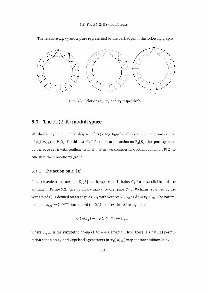
5.3. The SL(2,R) moduli space
The relations x4, x2 and x1, are represented by the dark edges in the following graphs:
Figure 5.3: Relations x4, x2 and x1 respectively.
5.3 The SL(2,R) moduli space
We shall study here the moduli space of SL(2,R)-Higgs bundles via the monodromy action
of π1(Areg) on P[2]. For this, we shall first look at the action on Z2[E], the space spanned
by the edge set E with coefficients in Z2. Then, we consider its quotient action on P[2] to
calculate the monodromy group.
5.3.1 The action on Z2[E]
It is convenient to consider Z2[E] as the space of 1-chains C1 for a subdivision of the
annulus in Figure 5.2. The boundary map ∂ to the space C0 of 0-chains (spanned by the
vertices of Γ) is defined on an edge e ∈ C1 with vertices v1, v2 as ∂ e = v1+ v2. The natural
map p :Areg → Σ[4g−4] introduced in (5.1) induces the following maps
π1(Areg)→ π1(Σ[4g−4])→ S4g−4 ,
where S4g−4 is the symmetric group of 4g − 4 elements. Thus, there is a natural permu-
tation action on C0 and Copeland’s generators in π1(Areg) map to transpositions in S4g−4.
81

Chapter 5. Monodromy of the SL(2,R) Hitchin fibration Hitchin fibration
Concretely, these generators are defined as transformations of Z2[E] as follows. The action
σe labelled by the edge e on another edge x is
σe(x) = x +< x , e > e, (5.6)
where < ·, · > is the intersection pairing. As this pairing is skew over Z, for any edge e one
has < e, e >= 0. Let G1 be the group of transformations of C1 generated by σe, for e ∈ E.
Proposition 5.11. The group G1 acts trivially on Z1 = ker(∂ : C1→ C0).
Proof. Consider a ∈ C1 such that ∂ a = 0, i.e., the edges of a have vertices which occur an
even number of times. By definition, σe ∈ G1 acts trivially on a for any edge e ∈ E non
adjacent to a. Furthermore, if e ∈ E is adjacent to a, then ∂ a = 0 implies that an even
number of edges in a is adjacent to e, and thus the action σe is also trivial on a.
We shall give an ordering to the vertices in Γ as in the figure below, and denote by
E′ ⊂ E the set of dark edges:
Figure 5.4: The subset E′ ⊂ E.
For (i, j) the edge between the vertices i and j, the set E′ is given by the natural succes-
sion of edges ei := (i, i+1) for i = 1, . . . , 4g−5, together with the edge e4g−4 := (4g−4, 1).
82

5.3. The SL(2,R) moduli space
Proposition 5.12. The reflections labelled by the edges in E′ ⊂ E generate a subgroup S′4g−4
of G1 isomorphic to the symmetric group S4g−4.
Proof. To show this result, one needs to check that the following properties characterising
generators of the symmetric group apply to the reflections labelled by E′:
(i) σ2ei= 1 for all i,
(ii) σeiσe j= σe j
σeiif j 6= i± 1,
(iii) (σeiσei+1
)3 = 1.
By equation (5.6), it is straightforward to see that the properties (i) and (ii) are satisfied by
σeifor all ei ∈ E. Indeed, let e be an edge in E and σe be its associated reflection. As
σe(x) = x+< x , e > e,
one has that
σ2e (x) = x+< x , e > e+< x , e > e = x .
Similarly, let ei and e j be two edges which do not intersect. Then
σeiσe j(x) = σei
(x+< x , e j > e j) = x+< x , e j > e j+< x , ei > ei ,
and as x+< x , e j > e j+< x , ei > ei is symmetric in i, j, one has
σeiσe j(x) = σe j
σei(x).
In order to check (iii) we shall consider all different options for edges adjacent to ei and
ei+1 when ei , ei+1 ∈ E′. These can be seen in the following figure:
83
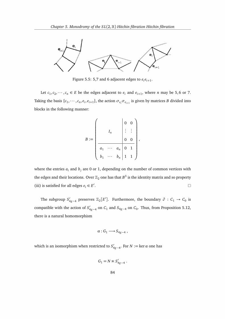
Chapter 5. Monodromy of the SL(2,R) Hitchin fibration Hitchin fibration
Figure 5.5: 5,7 and 6 adjacent edges to eiei+1.
Let c1, c2, · · · , cn ∈ E be the edges adjacent to ei and ei+1, where n may be 5,6 or 7.
Taking the basis c1, · · · , cn, ei , ei+1, the action σeiσei+1
is given by matrices B divided into
blocks in the following manner:
B :=
0 0
In...
...
0 0
a1 · · · an 0 1
b1 · · · bn 1 1
,
where the entries ai and b j are 0 or 1, depending on the number of common vertices with
the edges and their locations. Over Z2 one has that B3 is the identity matrix and so property
(iii) is satisfied for all edges ei ∈ E′.
The subgroup S′4g−4 preserves Z2[E′]. Furthermore, the boundary ∂ : C1 → C0 is
compatible with the action of S′4g−4 on C1 and S4g−4 on C0. Thus, from Proposition 5.12,
there is a natural homomorphism
α : G1 −→ S4g−4 ,
which is an isomorphism when restricted to S′4g−4. For N := kerα one has
G1 = N n S′4g−4 .
84
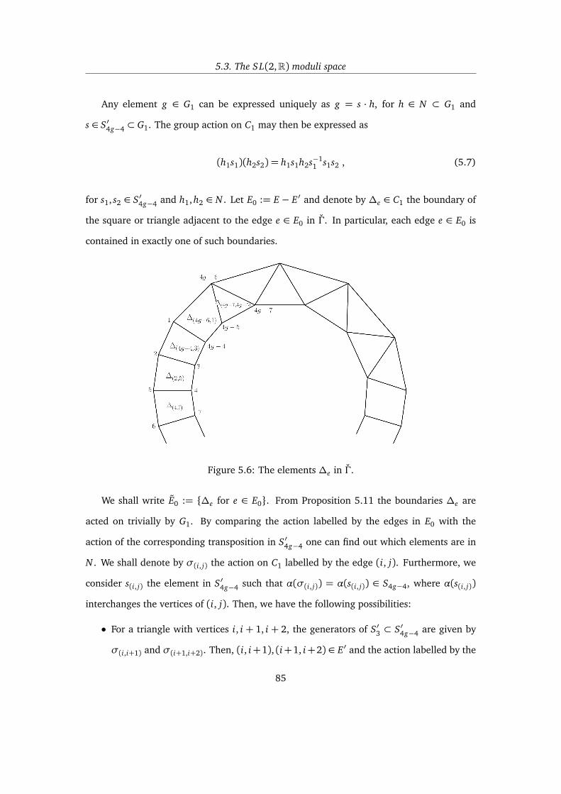
5.3. The SL(2,R) moduli space
Any element g ∈ G1 can be expressed uniquely as g = s · h, for h ∈ N ⊂ G1 and
s ∈ S′4g−4 ⊂ G1. The group action on C1 may then be expressed as
(h1s1)(h2s2) = h1s1h2s−11 s1s2 , (5.7)
for s1, s2 ∈ S′4g−4 and h1, h2 ∈ N . Let E0 := E − E′ and denote by ∆e ∈ C1 the boundary of
the square or triangle adjacent to the edge e ∈ E0 in Γ. In particular, each edge e ∈ E0 is
contained in exactly one of such boundaries.
Figure 5.6: The elements ∆e in Γ.
We shall write E0 := ∆e for e ∈ E0. From Proposition 5.11 the boundaries ∆e are
acted on trivially by G1. By comparing the action labelled by the edges in E0 with the
action of the corresponding transposition in S′4g−4 one can find out which elements are in
N . We shall denote by σ(i, j) the action on C1 labelled by the edge (i, j). Furthermore, we
consider s(i, j) the element in S′4g−4 such that α(σ(i, j)) = α(s(i, j)) ∈ S4g−4, where α(s(i, j))
interchanges the vertices of (i, j). Then, we have the following possibilities:
• For a triangle with vertices i, i + 1, i + 2, the generators of S′3 ⊂ S′4g−4 are given by
σ(i,i+1) and σ(i+1,i+2). Then, (i, i+1), (i+1, i+2) ∈ E′ and the action labelled by the
85

Chapter 5. Monodromy of the SL(2,R) Hitchin fibration Hitchin fibration
edge (i, i+ 2) ∈ E0 can be written as:
s(i,i+2) = σ(i+1,i+2)σ(i,i+1)σ(i+1,i+2) .
• For a square with vertices i, i + 1, i + 2, i + 3, the generators of S′4 ⊂ S′4g−4 are given
by σ(i,i+1),σ(i+1,i+2) and σ(i+2,i+3). In this case, the edges (i, i+1),(i+1, i+2), and
(i+ 2, i+ 3) are in E′, and the action labelled by (i, i+ 3) ∈ E0 can be written as:
s(i,i+3) = σ(i+2,i+3)σ(i+1,i+2)σ(i,i+1)σ(i+1,i+2)σ(i+2,i+3) .
Theorem 5.13. The action of σe labelled by e ∈ E on x ∈ C1 is given by
σe(x) = he · se (x) ,
where se ∈ S′4g−4 is the element which maps under α to the transposition of the two vertices of
e, and the action of he ∈ N is given by
he(x) =
x if e ∈ E′ ,
x+< e, x >∆e if e ∈ E0 .(5.8)
Proof. For e ∈ E′, one has σe ∈ S′4g−4. Furthermore, one can see that the action of σe
labelled by e ∈ E0 on an adjacent edge x is given by
σe(x) = x+< x , e > ei
= se(x) +∆e.
From Proposition 5.11, the boundary ∆e is acted on trivially by G1 and thus the above
86

5.3. The SL(2,R) moduli space
action is given by
he · se(x) = he(σe(x) +∆e) = he(x)+< x , ei > ei +∆e = σe(x),
whence proving the proposition.
Example 5.14. By definition, the action labelled by the edge e = (4g − 4,3) ∈ Γ, is given by
σe(i, j) = (i, j) + < (i, j), e > e. This is non-trivial only over adjacent edges. Consider the
action on the edge x = (4g − 4,1), which is σe(x) = x + e. This can be rewritten as
σe(x) = (1, 2) + (2, 3) + ∆e. (5.9)
On the other hand, by acting with elements in S′4g−4 we have
se = σ(2,3)σ(1,2)σxσ(1,2)σ(2,3),
and thus
se(x) = σ(2,3)σ(1,2)σxσ(1,2)(x)
= σ(2,3)σ(1,2)σx (x + (1,2))
= σ(2,3)σ(1,2)(1,2)
= σ(2,3)(1,2)
= (1, 2) + (2,3).
Comparing this with σe(x), since ∆e is invariant under se, we see that
se ·σe(x) = se((1, 2) + (2,3) + ∆e)
= se(se(x) + ∆e)
= x + ∆e.
87
Chapter 5. Monodromy of the SL(2,R) Hitchin fibration Hitchin fibration
Hence, for h(x) := x +∆e we have σe(x) = h · se(x).
Remark 5.15. Note that for e, e′ ∈ E0, the maps he and he′ satisfy
hehe′(x) = x+< x , e′ >∆e′+< e, x >∆e . (5.10)
In order to construct a representation for the action of π1(Areg) on C1, we shall begin
by studying the image B0 and the kernel Z1 of ∂ : C1→ C0.
5.3.2 The representation of G1
For y = (y1, . . . , y4g−4) ∈ C0, we define the linear map f : C0→ Z2 by
f (y) =4g−4∑
i=1
yi . (5.11)
Proposition 5.16. The image B0 of ∂ : C1 → C0 is formed by elements with an even number
of 1’s, i.e., B0 = ker f .
Proof. It is clear that B0 ⊂ ker f . In order to check surjectivity we consider the edges
ei ∈ C1 given by ei = (i, i + 1) ∈ E′, for i = 1, . . . , 4g − 5. Given the elements Rk ∈ B0 for
k = 2, · · · , 4g − 4 defined as
R2 := ∂ e1 = (1, 1,0, . . . , 0) ,
...
Rk := Rk−1+ ∂ ek−1 = (1, 0, . . . , 0, 1, 0, . . . , 0),
one may generate any distribution of an even number of 1’s. Hence, B0 = spanRk which
is the kernel of f .
Proposition 5.17. The image B0 and the kernel Z1 of the derivative ∂ : C1 → C0 have,
respectively, dimension 4g − 5 and 2g + 3.
88

5.3. The SL(2,R) moduli space
Proof. From Prop. 5.16 one has that dim(B0) = dim(ker f ) = 4g − 5. Furthermore, as
dim C1 = dim Z1+ dim B0, the kernel Z1 of ∂ has dimension 2g + 3.
Note that x1, x2, x4 ∈ Z1 and x5 /∈ Z1. From a homological viewpoint one can see that
x4 and ∆e for e ∈ E0 form a basis for the kernel Z1. We can extend this to a basis of C1 by
taking the edges
β ′ := ei = (i, i+ 1) for 1≤ i ≤ 4g − 5 ⊂ E′ ,
whose images under ∂ form a basis for B0, and hence a basis for a complementary subspace
V of Z1. We shall denote by β := β0,β ′ the basis of C1 for β0 = E0, x4.
In order to generate the whole group G1, we shall study the action of S′4g−4 by conjuga-
tion on N . Considering the basis β one may construct a matrix representation of the maps
heifor ei ∈ E = E0, E′.
Proposition 5.18. For e ∈ E, the matrix [he] associated to he in the basis β is given by
[he] =
I2g+3 Ae
0 I4g−5
,
where the (2g + 3)× (4g − 5) matrix Ae satisfies one of the following:
• it is the zero matrix for e ∈ E′,
• it has only four non-zero entries in the intersection of the row corresponding to ∆e and
the columns corresponding to an adjacent edge of e for e ∈ E0− u5, l6,
• it has three non-zero entries in the intersection of the row corresponding to ∆e and the
columns corresponding to an adjacent edge of e for e = u5, l6.
Proof. As we have seen before, for e ∈ E0 the map he acts as the identity on the elements of
β0. Furthermore, any edge e ∈ E0 − u5, l6 is adjacent to exactly four edges in β ′. In this
case he has exactly four non-zero elements in the intersection of the row corresponding to
89

Chapter 5. Monodromy of the SL(2,R) Hitchin fibration Hitchin fibration
∆e and the columns corresponding to edges in β ′ adjacent to e. In the case of e = u5, l6,
the edge e is adjacent to exactly 3 edges in β ′ and thus he has only 3 non-zero entries.
Recall that S′4g−4 preserves the space spanned by E′, and hence also the subspace V ,
and acts trivially on Z1. In the basis β the action of an element s ∈ S′4g−4 has a matrix
representation given by
[s] =
I2g+3 0
0 πs
,
where πs is the permutation action corresponding to s. Hence, for f ∈ E0 we may construct
the matrix for a conjugate of h f as follows:
[s][h f ][s]−1 =
I2g+3 0
0 πs
I2g+3 A f
0 I4g−5
I2g+3 0
0 π−1s
=
I2g+3 A f π−1s
0 I4g−5
.
Proposition 5.19. The normal subgroup N ⊂ G1 consists of all matrices of the form
H =
I2g+3 A
0 I4g−5
,
where A is any matrix whose rows corresponding to ∆e for e ∈ E0 − u5, l6 have an even
number of 1’s, the row corresponding to x4 is zero and the rows corresponding to ∆u5,∆l6
have any distribution of 1’s.
Proof. Given ei ∈ E0 − u5, l6, the matrix Aeihas only four non-zero entries in the row
corresponding to ∆ei. Thus, for g > 2 , there exist elements s1, s2 ∈ S′4g−4 with associated
permutations π1 and π2 such that the matrix Aei:= Aei
π−11 + Aei
π−12 has only two non-
zero entries in the row corresponding to ∆ei, given by the vector R5 defined in the proof of
90

5.3. The SL(2,R) moduli space
Proposition 5.16. Furthermore, by Remark 5.15, we have
[s1heis−11 s2hei
s−12 ] = [s1hei
s−11 ][s2hei
s−12 ]
=
I2g+3 Aeiπ−1
1
0 I4g−5
I2g+3 Aeiπ−1
2
0 I4g−5
=
I2g+3 Aei
0 I4g−5
.
Considering different s ∈ S′4g−4 acting on s1heis−11 s2hei
s−12 , one can obtain the matrices
Akei4g−5
k=2 with Rk as the only non-zero row corresponding to ∆ei:
A2ei=
0
1 1 0 . . . 0
0
, . . . , A4g−5ei
=
0
1 0 . . . 0 1
0
.
Thus, by composing the elements of N to which each Akei
corresponds, we can obtain any
possible distribution of an even number of 1’s in the only non-zero row. Similar arguments
can be used for the matrices corresponding to u5, l6 which in this case may have any number
of 1’s in the only non-zero row. Recalling Remark 5.15 we are then able to generate any
matrix A∈ N as described in the proposition.
From the decomposition of G1 and above results, we have:
Theorem 5.20. The representation of σ ∈ G1 in the basis β is given by
[σ] =
I A
0 π
, (5.12)
where π represents a permutation on Z4g−52 and A is any matrix whose rows corresponding to
91
Chapter 5. Monodromy of the SL(2,R) Hitchin fibration Hitchin fibration
∆e for e ∈ E0 − u5, l6 have an even number of 1’s, the row corresponding to x4 is zero and
the rows corresponding to ∆u5and ∆l6 have any distribution of 1’s.
5.3.3 The monodromy action of π1(Areg) on P[2]
As seen previously, P[2] can be obtained as the quotient of C1 by the four relations x1, x2, x4
and x5. It is important to note that these relations are preserved by the action of π1(Areg).
Furthermore, x1, x2, x4 ∈ Z1 and ∂ x5 = (1, 1, · · · , 1) ∈ B0. Hence, we have the following
maps
Z2g2∼=
Z1
< x1, x2, x4 >→ P[2]→
B0
< (1,1, · · · , 1)>∼= Z4g−6
2 . (5.13)
The monodromy group G0 is given by the action on the quotient P[2] induced by the action
of G1 on C1. Note that having x1, x2, x3, x5 = 0 implies
0 = x1+ x4 =∑
li∈E0
∆li , (5.14)
0 = x2+ x4 =∑
ui∈E0
∆ui, (5.15)
0 = x5+ x4 =∑
even
ui +∑
odd
li . (5.16)
Then, one may write
∆l6 =∑
li∈E0−l6
∆li , and ∆u5=
∑
li∈E0−u5
∆ui. (5.17)
Moreover, as x1 + x2 + x4 + x5 = 0, one can express the edge u6 in terms of elements in
β ′− u6.
Definition 5.21. For β0 := β0− x4,∆l6 ,∆u5 and β ′ := β ′− u6, let β := β0, β ′.
Proposition 5.22. The elements in β0 generate Z1/ < x1, x2, x4 > and β ′ generates a com-
plementary subspace in P[2].
92

5.3. The SL(2,R) moduli space
From the previous analysis, one obtains our main theorem, which gives an explicit
description of the monodromy action on P[2]:
Theorem 5.23. The representation of σ ∈ G0 in the basis β is given by
[σ] =
I2g A
0 π
, (5.18)
where
• π is the quotient action on Z4g−52 /(1, · · · , 1) induced by the permutation action of the
symmetric group S4g−4 on Z4g−52 ;
• A is any (2g)× (4g − 6) matrix with entries in Z2.
Proof. As seen before, the action of G0 on B0/ < ∂ x5 = (1, 1, · · · , 1) > is given by the
quotient action of the symmetric group. Furthermore, replacing ∆u5and ∆l6 by the sums
in (5.17), one can use similar arguments to the ones in Proposition 5.19 to obtain any
number of 1’s in all the rows of the matrix A.
Remark 5.24. The intersection pairing in the above analysis means that the previous theorem
gives an irreducible representation of the symplectic group Sp(4g − 6,Z2) ( the reader should
refer to the work of Gow and Kleshchev [GK99] for details).
Remark 5.25. We have seen in Proposition 5.11 that the action of G1 is trivial on Z1. More-
over, the space Z2[x1, x2, x4, x5] is preserved by the action of G1, and thus one can see that the
induced monodromy action on the 2g-dimensional subspace Z1/Z2[x1, x2, x4, x5] is trivial.
Geometrically, there are 22g sections of the Hitchin fibration given by choices of the square root
of K. These sections meet each Prym in 22g points which also lie in P[2]. Since we can lift a
closed curve by a section, these are acted on trivially by the monodromy.
93

Chapter 5. Monodromy of the SL(2,R) Hitchin fibration Hitchin fibration
The analysis of the monodromy action for other split real forms encounters many new
complications. Hence, in the following chapters we shall study principal G-Higgs bundles
and the corresponding Hitchin fibration considering a different approach.
94
Chapter 6
Spectral data for U(p, p)-Higgs
bundles
In previous chapters we constructed principal Higgs bundles from a Lie theoretic point of
view. In particular, in Chapter 4 we gave a description of the fixed point set of the involution
Θ : (E,Φ) 7→ (σ(E),−σ(Φ))
associated to split real forms, acting on the Higgs bundle moduli space for the correspond-
ing complex Lie group. These results were then used to study SL(2,R)-Higgs bundles via
the monodromy action in Chapter 5. For non-split real forms the fixed point set of the cor-
responding involution Θ does not give a covering of the regular locus of the Hitchin base.
Consequently, an alternative approach to the monodromy action needs to be used in order
to understand the geometric and topological properties of the corresponding Higgs bundles
moduli spaces.
In this Chapter we shall study the particular case of U(p, p) and SU(p, p)-Higgs bun-
dles over a compact Riemann surface Σ, and define the spectral data associated to them.
Many authors have studied connectivity for SU(p, p)-Higgs bundles by looking at the nilpo-
95
Chapter 6. Spectral data for U(p, p)-Higgs bundles
tent cone in the corresponding Hitchin fibration (see, among others, the work of Brad-
low, Garcia-Prada and Gothen [BG-PG03]). In contrast, here we obtain information about
U(p, p) and SU(p, p)-Higgs bundles via the regular fibres of the Hitchin fibration. One
should note that U(p, q)-Higgs bundles for p < q have Higgs fields of rank at most 2p.
Thus, the characteristic polynomial of Φ is reducible, and the induced spectral curve is
singular. It is natural then to consider separately the cases of p = q and p 6= q.
We begin this chapter by recalling the main properties of U(p, p)-Higgs bundles in Sec-
tion 6.1. Then, we study the spectral data for U(p, p)-Higgs bundles in Section 6.2, and
for SU(p, p)-Higgs bundles in Section 6.3. Some applications of these results are given in
Chapter 8, and following the analysis of SO(2m+ 1,C)-Higgs bundles given in Chapter 2
(see [Hit07]), we consider U(p, q)-Higgs bundles for p 6= q in Chapter 9.
6.1 U(p, p)-Higgs bundles
Recall that the unitary group U(p, p) of signature (p, p) is a non-compact real form of
GL(2p,C), and has maximal compact subgroup H = U(p)× U(p). The complexified Lie
algebra of H is h= gl(p,C)⊕ gl(p,C). For
Ip,p =
−Ip 0
0 Ip
,
the antilinear involution τ on gl(2p,C) which fixes u(p, p) is given by τ(X ) = −Ip,pX ∗ Ip,p.
Moreover, the involution relating the compact real structure and the non-compact real
structure u(p, p) on gl(2p,C) is σ(X ) = Ip,pX Ip,p. As seen in Chapter 3, the involution
σ induces an involution Θ : (E,Φ) 7→ (σ(E),−σ(Φ)) on the classical Higgs bundle moduli
spaceM . In this case, Θ is given by
Θ : (E,Φ) 7→ (E,−Φ).
96
6.1. U(p, p)-Higgs bundles
The isomorphism classes of U(p, p)-Higgs bundles are given by fixed points of the involution
Θ onM corresponding to vector bundles E which have an automorphism conjugate to Ip,p
sending Φ to −Φ, and whose ±1 eigenspaces have dimensions p and q.
By considering the Cartan involution on the complexified Lie algebra of U(p, p) one has
u(p, p)C = gl(2p,C) = (gl(p,C)⊕ gl(p,C)) + mC, where mC corresponds to the off diagonal
elements of gl(2p,C). Then, a principal U(p, p)-Higgs bundle (P,Φ) is given by a principal
HC-bundle P and a holomorphic section Φ of (P ×Ad mC)⊗ K .
Definition 6.1. A U(p, p)-Higgs bundle over Σ is a pair (E,Φ) where E = V ⊕W for V, W
rank p vector bundles over Σ, and the Higgs field Φ given by
Φ =
0 β
γ 0
, (6.1)
for β : W → V ⊗ K and γ : V →W ⊗ K.
Definition 6.2. An SU(p, p)-Higgs bundle is a U(p, p)-Higgs bundle (V ⊕W,Φ) for which the
vector bundles satisfy ΛpV ∼= ΛpW ∗.
6.1.1 The spectral curves
Consider a stable U(p, p)-Higgs pair (V⊕W,Φ), with Φ given as in Definition 6.1. Note that
tr Φn =
0 for n odd,
2tr(γβ)n/2 for n even.(6.2)
Thus the characteristic polynomial of Φ, whose coefficients are polynomials in tr(Φi), de-
fines a spectral curve ρ : S→ Σ in the total space X of K with equation
η2p + a1η2p−2+ . . .+ ap−1η
2+ ap = 0, (6.3)
97

Chapter 6. Spectral data for U(p, p)-Higgs bundles
where ai ∈ H0(Σ, K2i), and η is the tautological section of ρ∗K in X . By Bertini’s theorem
this curve is generically smooth, and thus in the remainder of this chapter we shall assume
S is smooth. The 2p-fold cover S has an involution η 7→ −η, which we shall denote by σ
following the notation of Chapter 2. The quotient of S by the action of σ defines a p-fold
cover ρ : S→ Σ in the total space of K2, whose equation is given by
ξp + a1ξp−1+ . . .+ ap−1ξ+ ap = 0, (6.4)
where ξ= η2 is the tautological section of ρ∗K2. Since S is the quotient of a smooth curve,
it is also smooth. We let π : S→ S be the double cover given by the above quotient:
S π2:1 //
ρ
2p:1
S.
p:1
ρ
Σ
(6.5)
We shall denote by gS and gS the genus of S and S, respectively. Since the cotangent bun-
dle has trivial canonical bundle, and the canonical bundle of K2 is ρ∗K−1, the adjunction
formula gives KS∼= ρ∗K2p and KS
∼= ρ∗K2p ⊗ ρ∗K−1. Thus, one has
gS = 4p2(g − 1) + 1, (6.6)
gS = (2p2− p)(g − 1) + 1. (6.7)
6.2 The spectral data of U(p, p)-Higgs bundles
A description of the fibres of the Hitchin fibration h : MGc → AGc , for classical complex
Lie groups Gc , was given in Chapter 2, following [Hit87a], in terms of line bundles on
associated curves. In the case of classical Higgs bundles of rank n, a point in the regular
locus of the Hitchin base defines a curve ρ : S → Σ in the total space X of the canonical
98
6.2. The spectral data of U(p, p)-Higgs bundles
bundle K , whose equation is given by
ηn+ a1ηn−1+ . . .+η1an−1+ an = 0,
where η is the tautological section of ρ∗K in X , and ai ∈ H0(Σ, K i). Given a line bundle M
on S, one could obtain a classical Higgs pair (E,Φ) by taking the direct image E := ρ∗M ,
and letting the Higgs field Φ be the map induced by the multiplication of the tautological
section
H0(ρ−1(U ), M)→ H0(ρ−1(U ), M ⊗ρ∗K),
for U an open set in the compact Riemann surface Σ. In this section we shall extend these
methods to study the fixed point set of the involution
Θ : (E,Φ) 7→ (E,−Φ),
in the classical Higgs bundles moduli spaceM , which correspond to U(p, p)-Higgs bundles.
In particular, we obtain the following correspondence.
Proposition 6.3. Given a U(p, p)-Higgs bundle with non-singular spectral curve one can con-
struct a pair (S, M) where
(a) the curve ρ : S → Σ is an irreducible non-singular 2p-fold cover of Σ given by the
equation
η2p + a1η2p−2+ . . .+ ap−1η
2+ ap = 0,
in the total space of K, where ai ∈ H0(Σ, K2i), and η is the tautological section of ρ∗K.
The curve S has an involution σ acting by σ(η) =−η;
(b) M is a line bundle on S such that σ∗M ∼= M.
99

Chapter 6. Spectral data for U(p, p)-Higgs bundles
Conversely, given a pair (S, M) satisfying (a) and (b), there is an associated stable U(p, p)-
Higgs bundle.
Proof. We shall begin by constructing the Higgs bundle induced by a given pair (S, M)
satisfying (a) and (b). Consider ρ : S → Σ and M as in (a) and (b), and denote the lifted
action of σ to M also by σ. Then, on an invariant open set ρ−1(U ) we may decompose
the sections of M into the invariant and anti-invariant parts:
H0(ρ−1(U ), M) = H0(ρ−1(U ), M)+⊕H0(ρ−1(U ), M)−.
From the definition of the direct image of a line bundle there is a similar decomposition of
H0(U ,ρ∗M) into
H0(U ,ρ∗M) = H0(U ,ρ∗M)+⊕H0(U ,ρ∗M)
−.
Thus, generically, we may write
ρ∗M = E+⊕ E−,
where E± are rank p vector bundles on Σ. At a point x such that ap(x) 6= 0, the involution
σ has no fixed points on ρ−1(x). Moreover, if x is not a branch point, ρ−1(x) consists of
2p points e1, . . . , ep,σe1, . . .σep. The fibre of the direct image is then isomorphic to Cp⊕Cp
with the involution (v, w) 7→ (w, v), so that the fibre of E+ is given by the invariant points
(v, v) and the one of E− is given by the anti-invariant points (v,−v).
In order to define the Higgs field associated to M , we follow the ideas done for the
classical case in Chapter 2 and consider the tautological section η of ρ∗K , which induces
the multiplication map
H0(ρ−1(U ), M)η−→ H0(ρ−1(U ), M ⊗ρ∗K). (6.8)
100
6.2. The spectral data of U(p, p)-Higgs bundles
By definition of direct image, this map gives the Higgs field
Φ : ρ∗M → ρ∗M ⊗ K .
Furthermore, as σ(η) =−η, the Higgs field Φ maps E+ 7→ E−⊗K and E− 7→ E+⊗K . Thus,
we may write
Φ =
0 β
γ 0
for γ : E+→ E− ⊗ K and β : E−→ E+ ⊗ K . Note that as we have considered an irreducible
curve S, there is no proper subbundle of E+ ⊕ E− which is preserved by Φ, and hence the
Higgs pair (E+⊕ E−,Φ) is a stable U(p, p)-Higgs bundle associated to (S, M).
Conversely, by considering a stable U(p, p)-Higgs bundle (E = V ⊕W,Φ) defined as
in Definition 6.1, one can obtain the induced pair (S, M) as follows. The characteristic
polynomial of Φ defines the curve S, which by stability is smooth and irreducible. We
have seen in Chapter 2 that the regular fibres of the Hitchin fibration for classical Higgs
bundles are isomorphic to the Picard variety of S. As a classical Higgs bundle, (E,Φ) has a
corresponding line bundle M on the spectral curve S. Since the involution σ acts trivially
on the equation of S, the fixed points correspond to the action on the Picard variety, and
thus σ∗M ∼= M . Hence, the pair (S, M) associated to the Higgs bundle (E,Φ) satisfies Item
(a) and Item (b) of Proposition 6.3.
By means of the 2-fold covering π : S→ S, the line bundle M from Proposition 6.3 can
be interpreted in terms of line bundles on the quotient curve S in the following way. Let V
be an open set in S. Then, the invariant and anti-invariant sections of the line bundle M on
S introduced in the Proposition 6.3 give a decomposition
H0(π−1(V ), M) = H0(π−1(V ), M)+⊕H0(π−1(V ), M)−.
101
Chapter 6. Spectral data for U(p, p)-Higgs bundles
By definition of direct image, there are two line bundles U1 and U2 on the quotient curve S
such that
H0(π−1(V ), M)+ ∼= H0(V , U1) and H0(π−1(V ), M)− ∼= H0(V , U2), (6.9)
and thus π∗M = U1 ⊕ U2. Therefore the pair (S, M) corresponding to the U(p, p)−Higgs
bundle (E,Φ), which satisfies Item (a) and Item (b) of Proposition 6.3, defines two associ-
ated line bundles U1 and U2 on the quotient curve S.
6.2.1 The associated invariants
Let (E = V ⊕ W,Φ) be a U(p, p)-Higgs bundle. By reduction to the maximal compact
subgroup, a flat U(p, p) bundle has two integer invariants. These invariants correspond to
the degrees v = deg V and w = deg W of the Higgs bundle (E,Φ). We shall see next how
they arise from the isomorphism σ∗M ∼= M . This isomorphism gives an action of +1 or −1
on the fixed points of the involution and defines one of the invariants:
Proposition 6.4. Let (V ⊕W,Φ) be a U(p, p)-Higgs bundle corresponding to a pair (S, M) as
in Proposition 6.3. For m the degree of M, and m the number of fixed points of the involution
σ for which it acts as −1 on M, the degrees v and w of V and W are given by
v =m− m
2+ (2p− 2p2)(g − 1),
w =m+ m
2− 2p2(g − 1).
Proof. Consider the line bundle M on S whose degree we denote by m and which corre-
sponds, through the previous analysis, to the pair (V ⊕W,Φ). In particular, we have that
ρ∗M = V ⊕W. The involution σ preserves M , and on its 4p(g − 1) fixed points it acts as
±1. We shall denote by m the number of points on which σ acts as −1. As noted before, in
102

6.2. The spectral data of U(p, p)-Higgs bundles
terms of the ±1 eigenspaces of σ we may write
H0(ρ−1(U ), M) = H0(ρ−1(U ), M)+⊕H0(ρ−1(U ), M)−
for an open setU ⊂ Σ. Furthermore, there is a similar decomposition of the sections of the
direct image of M on Σ:
H+ := H0(ρ−1(U ), M)+ ∼= H0(U , V ), (6.10)
H− := H0(ρ−1(U ), M)− ∼= H0(U , W ). (6.11)
Recall that for the 2p-fold cover ρ : S→ Σ, the degree of the direct image ρ∗M is given by
deg(ρ∗M) = deg(M) + (1− gS)− deg(ρ)(1− g). Then, we have that
v+w = degρ∗M = m+ (1− gS)− 2p(1− g)
= m+ 1− 1− 4p2(g − 1)− 2p(1− g)
= m+ (2p− 4p2)(g − 1),
and thus m= v+w+ (4p2− 2p)(g − 1).
Given L a line bundle over S, the involution σ acts trivially on the pull-back π∗L.
Furthermore, one may consider the tensor product M ⊗ π∗L for which the direct image
under π is given by
π∗(M ⊗π∗L) = π∗M ⊗ L.
For convenience we shall assume that the degree l := deg L is sufficiently large. Then,
H1(S, M ⊗π∗L) vanishes and thus one may use Riemann-Roch to calculate the dimension
of H0(S, M ⊗ π∗L). Over the fixed points of the involution, σ acts as +1 on π∗L and so
the involution acts as −1 on M ⊗π∗L for exactly m points. Thus, we may assume that the
degree m of M is sufficiently large to make H1(S, M) vanish.
103
Chapter 6. Spectral data for U(p, p)-Higgs bundles
In order to find the relation between m and the degrees v and w we shall first calculate
the dimension of the ±1-eigenspaces of σ on H0(S, M). Then, by means of Riemann-Roch
and Serre duality, we shall find the degrees of v and w of V and W in terms of m, and from
there give an equation for m. By Riemann-Roch and Serre duality one has that
dim H0(S, M) = deg M + 1− gS = m− 4p2(g − 1).
For h+ and h− the dimension of the ±1 eigenspaces of H0(S, M) respectively,
h++ h− = m− 4p2(g − 1).
Consider the Lefschetz number as defined in [AB68] associated to the involution σ on S,
which is given by:
L(σ) =∑
(−1)qtrace σ|H0,q(M)
= trace σ|H0(M)
= h+− h−.
From the holomorphic Lefschetz theorem [AB68, Theorem 4.12], we can express L(σ) as:
L(σ) =(−m) + (4p(g − 1)− m)
2
= 2p(g − 1)− m.
Note that as the Lefschetz number only depends on m, its value is the same for the line
bundles M and M ⊗π∗L.
The dimensions h+ and h− can then be obtained as follows:
h+ =m− 4p2(g − 1) + 2p(g − 1)− m
2=
m− m
2+ (p− 2p2)(g − 1),
h− =m− 4p2(g − 1)− 2p(g − 1) + m
2=
m+ m
2− (p+ 2p2)(g − 1).
104

6.2. The spectral data of U(p, p)-Higgs bundles
These equations may be considered when applying Riemann-Roch and Serre duality in
order to give an expression of the degrees v and w in terms of m and m:
v = h++ p(g − 1) =m− m
2+ (2p− 2p2)(g − 1),
w = h−+ p(g − 1) =m+ m
2− 2p2(g − 1).
Note that
w− v =m+ m
2− 2p2(g − 1)−
m− m
2+ (2p− 2p2)(g − 1)
= m− 2p(g − 1).
Hence, the number m can be expressed as m= w− v+ 2p(g − 1).
Remark 6.5. From the proof of Proposition 6.4, the parity of the degree of M and the number
of fixed points m over which σ acts as −1 need to be the same.
Remark 6.6. Throughout this chapter we have assumed that V and W were obtained via the
invariant and anti-invariant sections of M, respectively. However, this choice is arbitrary, and
interchanging the role of V and W corresponds to considering the involution −σ acting on
S. Moreover, considering −σ corresponds to taking the invariants (m, m), instead of (m, m),
where m= 4p(g − 1)− m.
The invariant m introduced in Proposition 6.4 gives the number of fixed points of σ
over which the involution acts as -1 on M , i.e., is the degree of a positive divisor of the
section ap = det(βγ) associated to a Higgs bundle (V ⊕W,Φ). Consider the line bundles
U1 and U2 on S as defined in (6.9), for which ρ∗U1 = V and ρ∗U2 = W . Then, the Higgs
field Φ = (β ,γ) induces two sections
b ∈ H0(S, U∗2 ⊗ U1⊗ρ∗K), and c ∈ H0(S, U∗1 ⊗ U2⊗ρ
∗K).
105

Chapter 6. Spectral data for U(p, p)-Higgs bundles
By stability of the Higgs bundle, if v ≥ w (otherwise one can interchange V and W ), the
section γ 6= 0 induces a non vanishing section c of U∗1⊗U2⊗ρ∗K , and thus defines a positive
divisor D of degree m associated to the Higgs bundle. We shall denote by [s] the divisor
associated to a section s.
Remark 6.7. Since D is a positive divisor of [ap], which has simple zeros and gives the rami-
fication points, one can think of it as a divisor on Σ as well as on ρ : S→ Σ, by identifying D
and Nm(D).
Note that since U1 and U2 are constructed via the invariant and anti-invariant sections
of M , respectively, the divisor D is given by the fixed points of the involution (the zeros of
ap) over which σ acts as −1 on M .
Remark 6.8. Interchanging the roles of V and W is equivalent to interchanging σ by −σ.
In this case, the associated triple is (S, M , D) where D is the divisor satisfying [ap] = D+ D,
which has degree m= 4p(g − 1)− m.
Note than when p = 1, the surface Σ and the curve S coincide. For p > 1, one may
express the degrees of the bundles U1 and U2 in the construction of the spectral data in
terms of the degrees of V and W , or in terms of the degree of M , as follows:
deg U1 = v + (2p2− 2p)(g − 1) =m
2−
m
2, (6.12)
deg U2 = w+ (2p2− 2p)(g − 1) =m
2+
m
2− 2p(g − 1). (6.13)
From the study of the spectral data for U(p, p)-Higgs bundles, we have the following
theorem:
Theorem 6.9. There is a one to one correspondence between U(p, p)-Higgs bundles with non-
singular spectral curve (V ⊕W,Φ) on a compact Riemann surface Σ of genus g > 1 for which
deg V > deg W, and triples (S, U1, D) where
106
6.2. The spectral data of U(p, p)-Higgs bundles
• S is a non-singular p-fold cover of Σ in the total space of K2 given by the equation
ξp + a1ξp−1+ . . .+ ap−1ξ+ ap = 0 for ai ∈ H0(Σ, K2i) ;
• U1 is a line bundle on S whose degree is deg U1 = deg V + (2p2− 2p)(g − 1);
• D is a positive subdivisor of the divisor of ap of degree m= deg W −deg V + 2p(g − 1).
Proof. From Proposition 6.3 and Proposition 6.4, it is left to show the equivalence between
the line bundles M and U1 satisfying the hypothesis, and the curves S and S.
Consider a pair (S, M) as in Proposition 6.3 and D a positive subdivisor of the divisor
of ap over which σ acts as −1 on M following Proposition 6.4. It was shown before that
the direct image π∗M on S = S/σ is decomposed into π∗M = U1 ⊕ U2, for U1 and U2 line
bundles on S satisfying
[D] = U∗1 ⊗ U2⊗ ρ∗K .
Note that for v > w, from equations (6.12)-(6.13) one has that deg U1 > deg U2. Hence,
considering the line bundle U1 of biggest degree, and identifying Picdeg U1(S) with Jac(S),
one can construct the triple (S, U1, D).
Conversely, consider a triple (S, U1, D) for ρ : S → Σ a smooth p-fold cover of Σ with
equation
ξp + a1ξp−1+ . . .+ ap−1ξ+ ap = 0,
for ai ∈ H0(Σ, K2i) and ξ the tautological section of ρ∗K2, and D a positive subdivisor
of zeros of ap. The line bundle U1 on S is considered in Jac(S) via the isomorphism
Picdeg U1(S)∼= Jac(S). Since, by [BNR, Remark 3.5], the section ap has simple zeros, follow-
ing Remark 6.8, we write [ap] = D+D, for D a positive divisor on Σ. Given the line bundle
U1 on S, we define the line bundle U2 also on S by
U2 = [D]⊗ U1⊗ρ∗K∗.
107

Chapter 6. Spectral data for U(p, p)-Higgs bundles
On S there is a natural rank 2 Higgs bundle (U1 ⊕ U2, Φ) whose Higgs field is obtained via
multiplication by ξ, the tautological section of ρ∗K2, giving
(U1⊕ U2)→ (U1⊕ U2)⊗ ρ∗K2.
The corresponding spectral curve of this K2-twisted Higgs bundle is the double cover
π : S → S and following the procedures of Chapter 2, there is a line bundle M on S
which is preserved by the involution σ on S (see [BNR] for details on spectral curves for
these twisted Higgs bundles). Moreover, its direct image has the direct sum decomposition
π∗M = U1 ⊕ U2 via the invariant and anti-invariant sections. Thus, one has the induced
pair (S, M), and by construction σ acts as −1 on M over the divisor D, whence proving the
proposition.
Remark 6.10. By interchanging the involutions σ and −σ, one can show that an equivalent
correspondence exists in the case of U(p, p)-Higgs bundles for which deg V < deg W.
Following [BG-PG03], we define the Toledo invariant τ(v, w) on U(p, p)-Higgs bundles
as the number
τ(v, w) = v−w. (6.14)
By considering the previous calculations, this invariant may be expressed as
τ(v, w) =−m+ 2p(g − 1).
Remark 6.11. By definition, m satisfies 0≤ m≤ 4p(g − 1), and thus
0≤ |τ(v, w)| ≤ 2p(g − 1),
which agrees in the case of U(p, p)-Higgs bundles with the general bounds given in [BG-PG03]
108
6.3. The spectral data of SU(p, p)-Higgs bundles
for the Toledo invariant.
One should note that U(p, p)-Higgs bundles (V⊕W,Φ) for deg V = deg W correspond to
m = 2p(g − 1), and the case of deg V > deg W (equivalently, deg V < deg W ) corresponds
to 0≤ m< 2p(g − 1) (equivalently, 2p(g − 1)< m≤ 4p(g − 1)).
6.3 The spectral data of SU(p, p)-Higgs bundles
We shall consider in this section SU(p, p)-Higgs bundles (E = V ⊕W,Φ) over Σ as given in
Definition 6.2. In particular, we have that v =−w and thus one can adapt Theorem 6.9 for
SU(p, p)-Higgs, to obtain the invariants
m = (4p2− 2p)(g − 1), (6.15)
m = 2 deg W + 2p(g − 1). (6.16)
Note that in this case not all triples (S, U1, D) satisfying the conditions of Theorem 6.9
have a corresponding stable SU(p, p)-Higgs bundle: the restriction ΛpV ∼= ΛpW ∗ does not
only constrain m and m but also the norm of the line bundles U1 and U2 on the quotient
curve S, and thus the divisor D. In the following subsections we study the implications of
the isomorphism ΛpV ∼= ΛpW ∗.
6.3.1 The condition ΛpV ∼= ΛpW ∗
In terms of the line bundles U1 and U2 on S, the condition ΛpV ∼= ΛpW ∗ may be written
as Λpρ∗U1∼= Λpρ∗U
∗2 . Considering the norm map Nm : Pic(S)→ Pic(Σ), the determinant
bundles of V and W can be expressed as follows [BNR, Section 4]:
ΛpV = Λpρ∗Ui = Nm(Ui)⊗ K−p(p−1) for i = 1, 2. (6.17)
109
Chapter 6. Spectral data for U(p, p)-Higgs bundles
One should note that we are identifying divisors of Σ and their corresponding line bundles.
The condition ΛpV ∼= ΛpW ∗ is equivalent to requiring
Nm(U1) =−Nm(U2) + 2p(p− 1)K , (6.18)
which is compatible with the degree calculations done in previous sections giving
deg(U1) =−deg(U2) + 4p(p− 1)(g − 1).
In terms of divisors on Σ, one has D = Nm U∗1 +Nm U2 + pK . Thus, from (6.18), the
condition for the Higgs bundle to be an SU(p, p)-Higgs bundle can be expressed as
2Nm U1 = p(2p− 1)K − D. (6.19)
Equation (6.19) can be rewritten as Nm ([D]⊗U21 ⊗ρ
∗K1−2p) = 0. The choice of U1 is thus
determined by the choice of an element in ker Nm, i.e., in the Prym variety Prym(S,Σ), and
thus one has the following description of the spectral data for SU(p, p)-Higgs bundles.
Proposition 6.12. The spectral data (S, U1, D) of a U(p, p)-Higgs bundle as in Theorem 6.9
corresponds to an SU(p, p)-Higgs bundle with deg V > deg W, if and only if the line bundle
U1 and the divisor D satisfy (6.19), i.e.,
2Nm U1 = p(2p− 1)K − D.
Remark 6.13. Recall from Chapter 2 that an SU(p, p)-Higgs bundle is a fixed point of the
involution Θ : (E,Φ) 7→ (E,−Φ) in the moduli space of SL(2p,C)-Higgs bundles. As such, the
corresponding line bundle M in the Jacobian variety of S for which ρ∗M = V ⊕W satisfies the
Prym conditions
M ⊗ρ∗K(2p−1)/2 ∈ Prym(S,Σ).
110

Chapter 7
Spectral data for Sp(2p, 2p)-Higgs
bundles
In previous chapters we studied G-Higgs bundles from different points of view. In particular,
in Chapter 6 we looked at the spectral data corresponding to U(p, p)-Higgs bundles in the
regular fibres of the Hitchin fibration. In this chapter we shall follow a similar approach
and consider Sp(2p, 2p)-Higgs bundles on a compact Riemann surface Σ as fixed points of
the involution
Θ : (E,Φ) 7→ (E,ΦT),
acting on the moduli space MSp(4p,C) of Sp(4p,C)-Higgs bundles. Moreover, Sp(2p, 2p)-
Higgs bundles can be seen as SU(2p, 2p)-Higgs bundles but, as we shall see, they corre-
spond to points in the singular fibres of the SL(4p,C) Hitchin fibration
h :MSL(4p,C)→ASL(4p,C),
fixed by the involution
Θsu : (E,Φ) 7→ (E,−Φ).
111

Chapter 7. Spectral data for Sp(2p, 2p)-Higgs bundles
Hence, by understanding the fixed point set we obtain information about the singular fibres
of the SL(4p,C)-Hitchin fibration.
We begin the chapter recalling the main properties of Sp(2p, 2p)-Higgs bundles and
describing their different associated curves. In Section 7.2 we study the relation between
Sp(2p, 2p)-Higgs bundles and vector bundles of rank 2, and define the spectral data asso-
ciated to stable Sp(2p, 2p)-Higgs bundles. In Chapter 8 we shall relate the spectral data to
a certain moduli space of parabolic vector bundles of rank 2 on a covering of Σ.
7.1 Sp(2p, 2p)-Higgs bundles
The symplectic Lie algebra sp(4p,C) is given by the set of 4p× 4p complex matrices A that
satisfy J2pA+ At J2p = 0 for
J2p =
0 I2p
−I2p 0
.
In this chapter we shall consider Higgs bundles for the real form Sp(2p, 2p) of the Lie group
Sp(4p,C), whose Lie algebra is
sp(2p, 2p) =
Z11 Z12 Z13 Z14
Zt12 Z22 Z t
14 Z24
−Z13 Z14 Z11 −Z12
Zt14 −Z24 −Z t
12 Z22
Zi, j complex matrices,
Z11, Z13, Z12, Z14 p× p matrices,
Z11, Z22 skew Hermitian,
Z13, Z24 symmetric
.
We have seen in Chapter 3 that Sp(2p, 2p)-Higgs bundles are fixed points of the invo-
lution
Θ : (E,Φ) 7→ (E,ΦT)
on Sp(4p,C)-Higgs bundles corresponding to vector bundles E which have an endomor-
phism f : E → E conjugate to Kp,p, sending Φ to ΦT as in Section 3.4.2, and whose ±1
112

7.1. Sp(2p, 2p)-Higgs bundles
eigenspaces are of dimension 2p, where
Kp,p =
0 0 −Ip 0
0 0 0 Ip
Ip 0 0 0
0 −Ip 0 0
.
Concretely, Sp(2p, 2p)-Higgs bundles are defined as follows:
Definition 7.1. An Sp(2p, 2p)-Higgs bundle is a pair (E,Φ) where E = V ⊕W for V and W
rank 2p symplectic vector bundles, and where the Higgs field is
Φ =
0 β
γ 0
for
β : W → V ⊗ K
γ : V →W ⊗ Kand β =−γT,
for γT the symplectic transpose of γ as in Section 3.4.2.
Following the approach of Chapter 6, we shall study the different curves associated to
an Sp(2p, 2p)-Higgs bundle.
7.1.1 The associated curves
Let K be the canonical bundle of the compact Riemann surface Σ, and X its total space with
projection ρ : X → Σ. Consider (V ⊕W,Φ) an Sp(2p, 2p)-Higgs bundle as in Definition 7.1.
Since Φ is an Sp(4p,C)-Higgs field, from Chapter 2, its characteristic polynomial is
det(x −Φ) = x4p + x4p−2a1+ x4p−4a2+ . . .+ x2a2p−1+ a2p.
113

Chapter 7. Spectral data for Sp(2p, 2p)-Higgs bundles
The above coefficients, which are given by polynomials in tr(Φi), define the spectral curve
of the Higgs field, whose equation is
P (η2) := η4p +η4p−2a1+η4p−4a2+ . . .+η2a2p−1+ a2p = 0, (7.1)
where η is the tautological section of the pullback of K to X , and ai ∈ H0(Σ, K2i). One may
also consider the maps γTγ and γγT, where
γγT : W →W ⊗ K2 ,
γTγ : V → V ⊗ K2 .
For y = x2, the characteristic polynomial of γγT and γTγ is
y2p + y2p−1a1+ y2p−2a2+ . . .+ ya2p−1+ a2p.
Hence, for ξ := η2, the coefficients of the above polynomial define the spectral curve of
γγT and γTγ, whose equation is
P (ξ) := ξ2p + ξ2p−1a1+ ξ2p−2a2+ . . .+ ξa2p−1+ a2p = 0, (7.2)
and which lives in the total space of K2.
Proposition 7.2. The divisors defining the curves (7.1) and (7.2) have multiplicity 2.
Proof. Let ω : V ∼= V ∗ be the symplectic form on the vector bundle V . The composition of
ω with the map γTγ : V ⊗ K−2→ V defines the section
Γ : V ⊗ K−2→ V ∗,
114
7.1. Sp(2p, 2p)-Higgs bundles
which is skew symmetric. As γTγ : V → V ⊗ K2 is a symplectically self adjoint operator,
det(ξ− γTγ) = det(ξω−1−Γ).
Moreover, since ξω−1 − Γ is skew symmetric, its determinant is the square of the corre-
sponding Pfaffian and ξ− γγT has even-dimensional eigenspaces. Therefore,
det(ξ− γTγ) = Pf2(ξω−1−Γ) := P(ξ)2.
The equation of the spectral curve (7.2) associated to γTγ can be rewritten as
ξp + b1ξp−1+ . . .+ bp−1ξ+ bp
2= 0,
for bi ∈ H0(Σ, K2i), and thus is reducible.
The same argument can be made for γγT and Φ, and thus the spectral curve of Φ has
equation
η2p + b1η2p−2+ . . .+ bp−1η
2+ bp
2= 0.
Consider a 2-dimensional generic eigenspace of γTγ, and let vi for i = 1, 2 be a basis of
eigenvectors such that γTγvi =−λ2vi , where λ 6= 0. Then, for wi := γvi/λ one has that
γγTwi = γγTγvi/λ=−γλ2vi/λ=−λ2wi ,
and thus wi is an eigenvector of γγT with eigenvalue −λ2. Moreover, the vector (vi , wi)
satisfies
0 −γT
γ 0
vi
wi
=
−γTwi
γvi
=
−γTγvi/λ
γvi
= λ
vi
wi
.
Hence, (vi , wi) is a λ-eigenvector of Φ for i = 1, 2.
Remark 7.3. For i = 1, 2, the vectors (vi ,−wi) span an eigenspace of Φ with eigenvalue −λ.
115

Chapter 7. Spectral data for Sp(2p, 2p)-Higgs bundles
Hence, there is an isomorphism between the 2-dimensional eigenspaces of Φ for eigenvalues +λ
and −λ, given by (vi , wi) 7→ (vi ,−wi). From here one can see, again, that the characteristic
polynomial of Φ is invariant under the map η 7→ −η.
Definition 7.4. We denote by ρ : S → Σ the 2p-fold cover of Σ in the total space of K whose
equation is
p(η2) := η2p + b1η2p−2+ . . .+ bp−1η
2+ bp = 0. (7.3)
Note that (7.3) defines a divisor of ρ∗K2p, and since a cotangent bundle has trivial
canonical bundle it follows that KS∼= ρ∗K2p. Hence,
gS = 4p2(g − 1) + 1.
Definition 7.5. We denote by ρ : S → Σ the p-fold cover of Σ in the total space of K2 whose
equation is
p(ξ) := ξp + b1ξp−1+ . . .+ bp−1ξ+ bp = 0, (7.4)
where bi ∈ H0(Σ, K2i). In particular, a2p = b2p.
The characteristic polynomials P (η2) and P (ξ) of Φ and γγT, respectively, can be
written as
P (η2) = p(η2)2 and P (ξ) = p(ξ)2.
The curve S has a natural involution σ(η) =−η, and taking the quotient of S by the action
of σ one obtains the curve S. In this case, since the canonical bundle of K2 is ρ∗K−1 the
adjunction formula gives
KS∼= ρ∗K2p ⊗ ρ∗K−1,
116

7.2. The spectral data of Sp(2p, 2p)-Higgs bundles
and thus one has that
gS = (2p2− p)(g − 1) + 1.
We have defined the following coverings of the compact Riemann surface:
S 2:1π
//
2p:1
ρ
Sρ
p:1Σ
From Proposition 7.2, all Sp(2p, 2p)-Higgs bundles have singular spectral curves, i.e.,
have reducible characteristic polynomial det(ρ∗Φ−η) = p(η2)2. Moreover, the map ρ∗Φ−η
has 2-dimensional cokernel. Thus, whilst in previous chapters we considered line bundles
on spectral curves, in this chapter we shall look at rank 2 vector bundles on the curve S,
which we require to be smooth.
7.2 The spectral data of Sp(2p, 2p)-Higgs bundles
In this section we shall analyse the relation between Sp(2p, 2p)-Higgs bundles and rank
2 vector bundles on the smooth curves S and S. Note that a rank 2 vector bundle M on
S which is preserved by the involution σ has an induced action of detσ on Λ2M over the
fixed points. If Λ2M is a pullback from S, then there are only two induced actions on the
bundle: the trivial action and the opposite one. The former case corresponds to σ having
equal eigenvalues on M over all fixed points, and the latter case corresponds to σ having
different eigenvalues over all fixed points.
Proposition 7.6. Let M be a vector bundle on the 2p-fold cover ρ : S→ Σ which is preserved
by the involution σ, and whose determinant bundle is given by detM ∼= ρ∗K2p−1. If the
involution σ acts with eigenvalues +1 and −1 on M over all fixed points, then ρ∗M = V ⊕W,
for V and W rank 2p symplectic vector bundles on Σ.
117

Chapter 7. Spectral data for Sp(2p, 2p)-Higgs bundles
Proof. Consider M a rank 2 vector bundle on ρ : S→ Σ for which Λ2M ∼= ρ∗K2p−1. By the
relative duality theorem [BNR], one has that
ρ∗(M)∗ ∼= ρ∗(KS ⊗ρ∗K−1⊗M∗)
∼= ρ∗(ρ∗K2p−1⊗M∗)
∼= ρ∗(ρ∗K2p−1⊗M ⊗Λ2M∗)
∼= ρ∗(M).
Similarly, taking the direct image in the 2-fold cover π : S→ S one has that
π∗(M)∗ ∼= π∗(KS ⊗π∗K−1
S⊗M∗)
∼= π∗(ρ∗K2p ⊗π∗K−1
S⊗M∗)
∼= π∗(ρ∗K2p ⊗π∗ρ∗K−2p+1⊗M∗)
∼= π∗(ρ∗K ⊗M∗)
∼= π∗(M)⊗ ρ∗K−2p+2.
This duality can be described explicitly in the following way. The 2-fold covering π defines
a map
dπ : K−1S → π∗K−1
S,
or equivalently, a section of KS ⊗π∗K−1S
. At a generic point x in S, for s and f sections of
M and KS ⊗π∗K−1S⊗M∗, respectively, there is a natural pairing
∑
y∈π−1(x)
< s, f >y
dπ, (7.5)
where < , > is the canonical pairing between M and M∗⊗ρ∗K with values on ρ∗K .
In the case of the double covering π : S → S, the duality in the proximity of a ramifi-
118

7.2. The spectral data of Sp(2p, 2p)-Higgs bundles
cation point can be seen following a similar approach to Example 2.13. Indeed, the fixed
points of the involution σ acting on S give the ramification points of the double cover
π : S → S. For U and U local neighbourhoods of S and S, respectively, and z a local
coordinate near a ramification point, the cover is given by
U → U
z 7→ z2 := w.
In a neighbourhood of a ramification point, a section of M looks like
sz(w) = h0(w) + zh1(w),
and a section of ρ∗K ⊗M∗ looks like
fz(w) = ζ0(w) + zζ1(w),
where h0, h1,ζ0 and ζ1 are vector valued. Thus, the space of sections of the direct image
π∗M is the direct sum of 2 copies of the vector valued holomorphic functions on U . We
shall denote by s−z(w) and f−z(w) the functions for −z. Then, for s(w) = (sz(w), s−z(w))
and f (w) = ( fz(w), f−z(w)), a concrete expression of the duality theorem in a neighbour-
hood of w0 is given by
< s(w), f (w)>S =∑
i=+z,−z
< si(w), fi(w)>dπ|i
=< ζ0(w) + zζ1(w), h0(w) + zh1(w)>
2z
+< ζ0(w)− zζ1(w), h0(w)− zh1(w)>
−2z
= < ζ1(w), h0(w)>+< ζ0(w), h1(w)> . (7.6)
119
Chapter 7. Spectral data for Sp(2p, 2p)-Higgs bundles
Since M is preserved by the involution σ, following the ideas of Chapter 6, its direct image
can be expressed as direct sum defined via the invariant and anti-invariant sections
π∗(M) = MV ⊕MW . (7.7)
Without loss of generality we let MV correspond to the invariant sections of M , and define
ρ∗MV = V and ρ∗MW = W. Since ρ = ρπ, we have ρ∗M = V ⊕W. Suppose that σ acted
at a fixed point only with +1 eigenvalues. Let h0(0) = ei and ζ0(0) = e j , for e1 = (1, 0) and
e2 = (0, 1). Since
MV ⊕MW∼= (M∗V ⊕M∗W )⊗ ρ
∗K2p−2,
the pairing between the factors can be seen as follows. Recall that σ sends z 7→ −z, and so
the trivial action at a fixed point would give
ei + ze j 7→ ei − ze j , (7.8)
for i, j = 1,2. This implies, in particular, that the pairing < , >S is degenerate on the
invariant sections defining V . Indeed, the invariant sections would be given by h1(0) = 0
and ζ1(0) = 0, which would make the pairing (7.6) vanish.
On the other hand, if the action of σ has different eigenvalues over the fixed points,
say +1 on (0, 1) and −1 on (1,0), then the invariant sections of M are spanned by (0,1)
and z(1,0) (and similarly for the invariant sections of ρ∗K ⊗M∗). Hence, in this case from
(7.6) the pairing < , >S is non degenerate over the invariant sections, where for constants
c j for j = 1, . . . , 4 we have
< s(0), f (0)>S = < c1(1, 0), c2(0,1)>+< c3(0, 1), c4(1, 0)>
= c1c2− c3c4. (7.9)
120
7.2. The spectral data of Sp(2p, 2p)-Higgs bundles
Similarly, from (7.6), one can see that in this case the pairing is non-degenerate over the
anti-invariant sections, which are spanned by (1,0) and z(0,1). Therefore, the bracket
< , >S pairs MV (and MW ) non degenerately with itself only if the involution σ acts with
different eigenvalues over a fixed point.
If σ acts with different eigenvalues, the non degenerate pairing induces skew isomor-
phisms
MV∼= M∗V ⊗ ρ
∗K2p−2 and MW∼= M∗W ⊗ ρ
∗K2p−2.
By the relative duality theorem, this implies that V and W are isomorphic to their duals.
Moreover, the isomorphisms are symplectic. Indeed, since, at a generic point, V is a direct
sum of p copies of MV , for each i = 1, . . . , p we have the skew symmetric pairing < , >iS,
and thus we define the natural skew symmetric pairing on the direct image V = ρ∗MV
given byp∑
i=1
< , >iS
dρ.
The symplectic structure on W is defined in a similar fashion.
A rank 2 vector bundle M satisfying Proposition 7.6 defines a symplectic Higgs field
on Σ in the following way. Consider the tautological section η of ρ∗K , and the induced
multiplication map
H0(ρ−1(U ), M)η // H0(ρ−1(U ), M ⊗ρ∗K), (7.10)
for U an open set in Σ. By the definition of direct image, this map gives the Higgs field
Φ : ρ∗M → ρ∗M⊗K . Since V and W are the images of invariant and anti-invariant sections
respectively, Φ is a symplectic Higgs field which maps V 7→W ⊗ K and W 7→ V ⊗ K .
Conversely, starting with a symplectic Sp(2p, 2p)-Higgs bundle one can define a rank 2
vector bundle on the associated 2p-fold cover ρ : S → Σ, such that it is preserved by the
natural involution on S, and it is acted on by the involution with different eigenvalues over
121

Chapter 7. Spectral data for Sp(2p, 2p)-Higgs bundles
the fixed points:
Proposition 7.7. Each Sp(2p, 2p)-Higgs bundle on Σ with smooth curve S, defines a rank 2
vector bundle on S of determinant ρ∗K2p−1 which is preserved by the involution σ and acted
by as +1 and −1 over all fixed points.
Proof. Consider the map in S induced by the Sp(2p, 2p)-Higgs bundle
ρ∗Φ : ρ∗E→ ρ∗E ⊗ρ∗K .
As seen previously, there is a canonically defined vector bundle of rank 2 on S given by
M := coker(ρ∗Φ−η).
Since the ramification divisor of ρ : S→ Σ is a section of ρ∗K2p−1, from [BNR], the vector
bundle M fits in the exact sequence
0 // M ⊗ρ∗K−2p+1 // ρ∗Eρ∗Φ−η// ρ∗(E ⊗ K) // M ⊗ρ∗K // 0. (7.11)
Dialysing the above sequence and tensoring by ρ∗K , via the identification with the sym-
plectic form one has
0 // M∗ // ρ∗Eρ∗Φ+η// ρ∗E ⊗ρ∗K // M∗⊗ρ∗K2p // 0.
Since σ : η 7→ −η, the vector bundle M∗ for eigenvalue −η is transformed to
σ∗M∗ ∼= M ⊗ρ∗K−2p+1
for eigenvalue η. By Remark 7.3 there is an isomorphism between these two spaces and
122
7.2. The spectral data of Sp(2p, 2p)-Higgs bundles
thus σ∗M ∼= M , i.e., the vector bundle M is preserved by the involution σ, and
M ∼= M∗⊗ρ∗K2p−1.
Thus, Λ2M = ρ∗K2p−1, as in the hypothesis of Proposition 7.6.
We shall now understand how the involution σ acts on M at a fixed point. Let w be a
local coordinate on Σ where at w = 0 the Higgs field is singular. Since S is smooth, γ drops
rank by 1 and we can find bases of V and W such that γ is
γ=
0 w 0 . . . 0
1 0 0 . . . 0
0 0 1 . . . 0...
......
. . ....
0 0 0 0 1
. (7.12)
This leads to a local form for the Higgs field Φ which is given by a non-singular component
times
0 0 0 w
0 0 1 0
0 w 0 0
1 0 0 0
. (7.13)
Without loss of generality, we shall let Φ equal the above form, in which case a local coor-
dinate η on S corresponds to w = η2. The rank 2 vector bundle M on S may be expressed
as M = coker(ρ∗Φ−η) = ker(ρ∗Φ−η)t .
Following the approach of Proposition 7.6, consider v1 = (1, 0) and v2 = (0, 1) in the
123

Chapter 7. Spectral data for Sp(2p, 2p)-Higgs bundles
−η2-eigenspace of γTγ and let
w1 := γv1/η.=
0 w
1 0
1
0
1
η=
0
1/η
, (7.14)
w2 := γv2/η.=
0 w
1 0
0
1
1
η=
η
0
. (7.15)
Then, as seen previously, the η-eigenspace of Φ is spanned by x1 := (v1, w1) = (1, 0,0, 1/η)
and x2 := (v2, w2) = (0, 1,η, 0), whilst the −η-eigenspace of Φ is spanned by the vectors
y1 := (v1,−w1) = (1, 0,0,−1/η) and y2 := (v2,−w2) = (0, 1,−η, 0). As η goes to zero the
eigenspace is spanned by (0,0, 0,1) and (0,1, 0,0) in the first case, and by (0,0, 0,−1) and
(0,1, 0,0) in the second. By Remark 7.3 the eigenspaces are identified via an isomorphism
Ax1 = y1 and Ax2 = y2, and thus A(ηx1) = ηy1. As η goes to zero, the two spaces coincide
and ηx1→ (0,0, 0,1) and ηy1→−(0,0, 0,1). Hence, the limit of the isomorphism between
the two eigenspaces is −1 on the first factor and +1 on the second, i.e., the action of σ has
different eigenvalues, proving the proposition.
Remark 7.8. If a rank 2 vector bundle M on S preserved by σ and with determinant ρ∗K2p−1
is acted by the involution as +1 over all fixed points, or −1 over all fixed points, then its direct
image would not induce a symplectic Higgs bundle. In fact, the map Φ in this case is given by
Φ =
0 0 w 0
0 0 0 w
1 0 0 0
0 1 0 0
, (7.16)
which is not of the correct form since if γ becomes singular so should γT .
124
7.2. The spectral data of Sp(2p, 2p)-Higgs bundles
7.2.1 Stability conditions
The relation between the stability of the rank 2 vector bundles on S introduced in Propo-
sition 7.6 and Proposition 7.7, and stability of the corresponding Sp(2p, 2p)-Higgs bundles
on Σ is given as follows.
Proposition 7.9. An Sp(2p, 2p)-Higgs bundle on Σ with smooth curve S is stable if and only
if its corresponding rank 2 vector bundle M on S is stable.
Proof. Under the above hypothesis, the square root of the characteristic polynomial of an
Sp(2p, 2p)-Higgs bundle (E := ρ∗M ,Φ) is an irreducible polynomial p(η2) defining the
smooth curve S. Since the characteristic polynomial of (E,Φ) restricted to any invariant
subbundle must divide det(η−ρ∗Φ) = p(η2)2, the only invariant subbundles of E are rank
2p vector bundles F corresponding to the factor p(η2).
Since there are no invariant subbundles of F , the restriction ΦF of the Higgs field to F
gives a rank 2p classical Higgs bundle (F,ΦF ) which is stable. Moreover, by construction
its spectral curve is given by the equation p(η2) = 0, i.e., by the 2p-fold cover S. From
Chapter 2, there is a line bundle L on S for which ρ∗L = F . Since F ⊂ E = ρ∗M , the line
bundle L is a subbundle of the rank 2 vector bundle M . Hence, for M such that ρ∗M = E,
the invariant subbundles of E correspond to line subbundles L ⊂ M on S.
The vector bundle M is stable if and only if for all line subbundles L ⊂ M one has that
µ(L)< µ(M), or equivalently, that
degL < (2p2− p)(2g − 2).
Hence, M is stable if and only if the direct image of invariant subbundles satisfies
degρ∗L = degL+ (1− gS)− 2p(1− g)
= degL+ (2p− 4p2)(g − 1)< 0.
125
Chapter 7. Spectral data for Sp(2p, 2p)-Higgs bundles
Since the vector bundle ρ∗M has degree zero, if M is stable, the direct image ρ∗L does not
make the Higgs bundle unstable. Conversely, if the Higgs bundle is stable, all its subbundles
are of the form ρ∗L for L ⊂ M , and satisfy degρ∗L < 0. Hence, in this case one has
degL < (2p2 − p)(2g − 2) and thus M is stable. Therefore, the vector bundle M on S is
stable if and only if the induced Higgs pair (E := ρ∗M ,Φ) on Σ is stable.
The spectral data associated to Sp(2p, 2p)-Higgs bundles is thus described as follows.
Theorem 7.10. Each stable Sp(2p, 2p)-Higgs bundle (E = V ⊕W,Φ) on a compact Riemann
surface Σ of genus g ≥ 2 for which p(η2) = 0 defines a smooth curve, has an associated pair
(S, M) where
(a) the curve ρ : S→ Σ is a smooth 2p-fold cover of Σ given by the equation
η2p + b1η2p−2+ . . .+ bp−1η
2+ bp = 0,
in the total space of K, where bi ∈ H0(Σ, K2i), and η is the tautological section of ρ∗K.
The curve S has a natural involution σ acting by η 7→ −η;
(b) the vector bundle M is a rank 2 vector bundle on the smooth curve ρ : S → Σ with
determinant bundle Λ2M ∼= ρ∗K−2p+1, and such that σ∗M ∼= M. Over the fixed points
of the involution, the vector bundle M is acted on by σ with eigenvalues +1 and −1.
Conversely, a pair (S, M) satisfying (a) and (b) induces a stable Sp(2p, 2p)-Higgs bundle
(ρ∗M = V ⊕W,Φ) on the compact Riemann surface Σ.
7.2.2 Dimensional calculations via the spectral data
Through dimensional calculations, we shall show here that the space of Sp(2p, 2p)-Higgs
bundles satisfying the hypothesis of Theorem 7.10 sits inside the moduli space MSp(2p,2p)
of Sp(2p, 2p)-Higgs bundles as a Zariski open set. Recall that the dimension of the space of
126

7.2. The spectral data of Sp(2p, 2p)-Higgs bundles
stable Sp(4p,C)-Higgs bundles is
dimMSp(4p,C) = dimSp(4p,C)(g − 1) = 4p(4p+ 1)(g − 1).
Remark 7.11. Since the dimension of the real group Sp(2p, 2p) is 2p(4p+ 1), the expected
dimension of the moduli space of Sp(2p, 2p)-Higgs bundles is
dimMSp(2p,2p) = 2p(4p+ 1)(g − 1).
Let N be the moduli space of semi-stable rank 2 vector bundles on S with fixed deter-
minant bundle ρ∗K2p−1, and V a representative of a point in N . Then, the tangent space
of N at [V ] is
TN[V ] ∼= H1(S, End0V ).
Note that the dimension ofN is dimN = 3gS−3= 12p2(g−1). OnN there is an induced
action of σ, and hence one may consider N σ, the subspace of fixed isomorphism classes
of vector bundles. From [AG06, Section 2], any point in the moduli space N fixed by σ
can be represented by a semi-stable bundle with an action of σ, covering the action on S.
Moreover, since the action of σ extends to an action σ on the tangent space TN , one has
dimN σ = dimH1(S, End0V )+,
for H1(S, End0V )+ the fixed set of σ.
Proposition 7.12. The dimension of the parameter space of Sp(2p, 2p)-Higgs bundles as in
Theorem 7.10 is, as expected, 2p(4p+ 1)(g − 1).
Proof. Recall from Theorem 7.10 that Sp(2p, 2p)-Higgs bundles satisfying the hypothesis
have an associated pair (S, M). Hence, via the spectral data (S, M) it is sufficient to show
that the dimension of the spaceN σ of rank 2 vector bundles preserved by the involution σ,
127
Chapter 7. Spectral data for Sp(2p, 2p)-Higgs bundles
together with the dimension of the parameter space defining S sum up to 2p(4p+1)(g−1).
From its construction, the curve S is defined by the coefficients bi ∈ H0(Σ, K2i), and thus
the dimension of the parameter space is given by
dim
p⊕
i=1
H0(Σ, K2i)
!
=p∑
i=1
dim
H0(Σ, K2i)
=p∑
i=1
(4i− 1)(g − 1)
= (2p2+ p)(g − 1).
Hence, to prove the proposition one needs to show that the dimension of N σ satisfies
dim(N σ) = dimMSp(2p,2p)− (2p2+ p)(g − 1)
= 2p(4p+ 1)(g − 1)− (2p2+ p)(g − 1)
= (8p2+ 2p− 2p2− p)(g − 1)
= (6p2+ p)(g − 1)
Since from Theorem 7.10 the action of σ on V maps (v1, v2) 7→ (v1,−v2), the induced action
on End0V is given by
1 0
0 −1
a b
c −a
1 0
0 −1
=
a −b
−c −a
,
and thus it can be expressed in a suitable basis as
σ :=
1 0 0
0 −1 0
0 0 −1
. (7.17)
128
7.2. The spectral data of Sp(2p, 2p)-Higgs bundles
By means of σ and its action on H1(S, End0V ), we shall study the dimension
dimN σ = dimH1(S, End0V )+
through the Lefschetz number Lσ associated to σ on End0V as defined in [AB68]. By
[AB68, Eq. 4.11], the number Lσ is given by
Lσ = trace σ|H0(S,End0(V ))− trace σ|H1(S,End0(V )).
By stability, dimH0(S, End0V ) = 0 and hence
Lσ = −trace σ|H1(S,End0(V ))
= −dimH1(S, End0(V ))++ dimH1(S, End0(V ))
−.
Furthermore, by [AB68, Theorem 4.12] we have that
Lσ =∑
p f i xed
trace σ|End0Vp
det(1− dσ)=∑
p f i xed
trace σ|End0Vp
2.
Since trace σ|End0Vp=−1 over all 4p(g − 1) fixed points, one has that
Lσ =−2p(g − 1).
This implies that
−dimH1(S, End0(V ))++ dimH1(S, End0(V ))
− =−2p(g − 1).
By Riemann-Roch and Serre duality
dimH1(S, End0(V ))++ dimH1(S, End0(V ))
− = 12p2(g − 1),
129

Chapter 7. Spectral data for Sp(2p, 2p)-Higgs bundles
Thus, the dimension of N σ is given by
dim(N σ) = dimH1(S, End0(V ))+ = (6p2+ p)(g − 1),
whence the result follows.
Since the locus in ASp(4p,C) defining singular curves S is given by algebraic conditions,
the space of isomorphism classes of Higgs bundles (E,Φ) satisfying the conditions of Theo-
rem 7.10 is included inMSp(2p,2p) as a Zariski open set.
130
Chapter 8
Applications
In this chapter we shall describe some applications of the results given in Chapters 5-7.
In Section 8.1 we calculate the number of connected components of the moduli space of
SL(2,R)-Higgs bundles (see [Hit87], [Go88] ) via the monodromy action studied in Chap-
ter 5. In Section 8.2 we give a new geometric description of the connected components
of the moduli space of U(p, p) and SU(p, p)-Higgs bundles which intersect the generic fi-
bres of the corresponding Hitchin fibration. Finally, in Section 8.3 we give new results on
connectivity for the moduli space of stable Sp(2p, 2p)-Higgs bundles via the spectral data
given in Chapter 7.
8.1 The moduli space of SL(2,R)-Higgs bundles
Let M be the moduli space of SL(2,C)-Higgs bundles. From Theorem 4.12, the intersec-
tion of the moduli spaceMSL(2,R) of SL(2,R)-Higgs bundles with the smooth fibres of the
Hitchin fibration
h :M →A
is the space of elements of order two, giving a covering of the regular locus inA . Hence, a
natural way of obtaining information about the topology of the moduli spaceMSL(2,R) is via
131
Chapter 8. Applications
the monodromy action of the covering. In this section we calculate the number of connected
components of MSL(2,R) via Theorem 5.23, and thus describe the connected components
of the space of surface group representations into SL(2,R). We shall begin by studying
the orbits of the monodromy action in Section 8.1.1, and then relate this analysis to the
connected components of the moduli space of SL(2,R)-Higgs bundles in Section 8.1.2.
Since we consider the moduli spaceMSL(2,R) as sitting insideM , as mentioned in Chap-
ter 3, two real representations may be conjugate in the space of complex representations
but not by real elements. Indeed, if A is in GL(2,R) and detA= −1 then iA is in SL(2,C)
and conjugates SL(2,R) to itself. Thus, flat SL(2,R) bundles can be equivalent as SL(2,C)
bundles but not as SL(2,R) bundles. In particular, since A changes orientation in R2 it will
take Euler class k to Euler class −k.
In the remainder of the section we first calculate the number of connected components
ofMSL(2,R) via the inclusionMSL(2,R) ⊂M , and then add the number of connected com-
ponents corresponding to −k which could not be seen through the monodromy analysis.
8.1.1 The orbits of the monodromy action
Recall from Theorem 5.23 that for G0 the monodromy group, the representation of σ ∈ G0
in the basis β as defined in Definition 5.21, is given by
[σ] =
I2g A
0 π
, (8.1)
where π is the quotient action on Z4g−52 /(1, · · · , 1) induced by the permutation represen-
tation on Z4g−52 , and A is any (2g)× (4g − 6) matrix with entries in Z2. We shall denote
by G(s,x) the orbit of (s, x) ∈ P[2] ∼= Z2g2 ⊕ Z
4g−62 under the action of G0. For g ∈ G0, the
induced action on (s, x) is given by
g · (s, x)t =
I A
0 π
s
x
=
s+ Ax
πx
. (8.2)
132

8.1. The moduli space of SL(2,R)-Higgs bundles
Proposition 8.1. The action of G0 on P[2] has 22g + g − 1 different orbits.
Proof. The matrices A have any possible number of 1’s in each row, and so for x 6= 0 any
s′ ∈ Z2g2 may be written as s′ = s + Ax for some A. Hence, the number of orbits G(s,x) for
x 6= 0 is determined by the number of orbits of the action in Z4g−62 defined by ξ : x → πx .
The map ξ permutes the non-zero entries of x and thus the orbits of this action are given
by elements with the same number of 1’s.
From equation (5.13) the space Z4g−62 can be thought of as vectors in Z4g−4
2 with an
even number of 1’s, modulo (1, . . . , 1). Thus, for x ∈ Z4g−62 and x 6= 0, each orbit ξx is
defined by a constant m such that x has 2m non-zero entries, for 0 < 2m ≤ 4g − 4. Let
us call x ∈ Z4g−6 the element defined by the constant m such that 2m = (4g − 4)− 2m.
With this notation, we can see that x and x belong to the same equivalence class in Z4g−62 .
Note that for m 6= g − 1,2g − 2, the corresponding x is equivalent to x under ξ and thus
in this case there are g − 2 equivalent classes ξx . Then, considering the equivalence class
for m = g − 1, one has g − 1 different classes for the action of ξ. From equation (8.2), the
action of G0 on an element (s, 0) ∈ P[2] is trivial. Thus, in this case one has 22g different
orbits of G0.
Recall that the fixed point set in M of the involution Θ is given by the moduli space
of semistable SL(2,R)-Higgs bundles. As an application of our results, we shall study
the connected components corresponding to stable and strictly semistable SL(2,R)-Higgs
bundles. In particular, we shall check that no connected component of the moduli space
MSL(2,R) lies entirely over the discriminant locus ofA .
8.1.2 Connected components ofMSL(2,R)
The bundle of P[2] is a finite covering of Areg of degree 26g−6. Considering two points p
and q which are in the same orbit under the monodromy action, there is a path in Areg
133
Chapter 8. Applications
whose action connects them. The horizontal lift of the path inAreg is a path in P[2] which
connects these two points. Hence p and q are in the same connected component of the
fixed point submanifold of Θ : (E,Φ) 7→ (E,−Φ).
Since SL(2,R) is isomorphic to SU(1, 1), a stable SL(2,C)-Higgs bundle (E,Φ) whose
isomorphism class is fixed by the involution Θ : (E,Φ) 7→ (E,−Φ) is given by an SU(1,1)-
Higgs bundle, and thus from Chapter 3 the Higgs field can be expressed as
Φ =
0 β
γ 0
∈ H0(Σ, End0(E)⊗ K). (8.3)
In particular, Θ acts on E via transformations of the form
±
i 0
0 −i
. (8.4)
In the case of strictly semistable Higgs bundles, the following Proposition applies:
Proposition 8.2. Any point representing a strictly semistable Higgs bundle inM fixed by Θ
is in the connected component of a Higgs bundle with zero Higgs field.
Proof. The moduli spaceM is the space of S-equivalence classes of semistable Higgs bun-
dles. A strictly semistable SL(2,C)-Higgs bundle (E,Φ) is represented by E = V ⊕ V ∗ for a
degree zero line bundle V , and
Φ =
a 0
0 −a
for a ∈ H0(Σ, K).
If V 2 is nontrivial, one has an SL(2,R)-Higgs bundle only for Φ = 0, which corresponds
to a flat connection with holonomy in the group SO(2) ⊂ SL(2, R). If V 2 is trivial then
the automorphism (u, v) 7→ (v,−u) takes Φ to −Φ, corresponding to a flat bundle with
134

8.1. The moduli space of SL(2,R)-Higgs bundles
holonomy in R∗ ⊂ SL(2,R). By scaling Φ to zero this is connected to the zero Higgs field.
The differential a can be continuously deformed to zero by considering ta for 0 ≤ t ≤ 1.
Hence, by stability of line bundles, one can continuously deform (E,Φ) to a Higgs bundle
with zero Higgs field via strictly semistable pairs.
In the case of stable SL(2,R)-Higgs bundles we have the following result:
Proposition 8.3. Any stable SL(2,R)-Higgs bundle is in a connected component which inter-
sectsMreg .
Proof. Let (E = V ⊕ V ∗,Φ) be a stable SL(2,R)-Higgs bundle with
Φ =
0 β
γ 0
∈ H0(Σ, End0(E)⊗ K),
and d := deg V ≥ 0. Stability implies that the section γ ∈ H0(Σ, V−2K) is non-zero, and
thus 0 ≤ 2d ≤ 2g − 2. Moreover, the section β of V 2K can be deformed continuously to
zero.
The section γ defines a divisor [γ] in the symmetric product S2g−2−2dΣ. As this space
is connected, one can continuously deform the divisor [γ] to any [γ] composed of distinct
points. For a ∈ Areg with zeros x1, . . . , x4g−4, we may deform [γ] to [γ] given by the
points x1, . . . , xn ∈ Σ for n := 2g − 2− 2d, and such that γ is a section of U−2K for some
line bundle U .
The complementary zeros xn+1, . . . , x4g−4 of a form a divisor of U2K . Any section
β with this divisor can be reached by continuously deforming [β] from zero to the set
xn+1, . . . , x4g−4. Hence, we may continuously deform any stable Higgs bundle given by
(V ⊕ V ∗,Φ = β ,γ) to (U ⊕ U∗, Φ = β , γ) inMreg .
The above analysis establishes that the number of connected components of the fixed
point set of the involution Θ on M is less than or equal to the number of orbits of the
135
Chapter 8. Applications
monodromy group in P[2]. A flat SL(2,R)-Higgs bundle has an associated RP1 bundle
whose Euler class k is a topological invariant which satisfies the Milnor-Wood inequality
−(g − 1) ≤ k ≤ g − 1. In particular, SL(2,R)-Higgs bundles with different Euler class
lie in different connected components M kSL(2,R) of the fixed point set of Θ. Moreover, for
k = g − 1,−(g − 1) one has 22g connected components corresponding to the so-called
Hitchin components. Hence, the lower bound to the number of connected components of
the fixed point set of the involution Θ for k ≥ 0 is 22g + g − 1. As this lower bound equals
the number of orbits of the monodromy group on the fixed points of Θ on Mreg , one has
that the closures of these orbits can not intersect.
Since we consider k ≥ 0, the number of connected components of the fixed points of
the involution
Θ : (E,Φ) 7→ (E,−Φ)
onMreg is equal to the number of orbits of the monodromy group on the points of order
two of the regular fibres Mreg , i.e. 22g + g − 1. From the above analysis, one has the
following application of Theorem 5.23:
Proposition 8.4. The number of connected components of the moduli space of semistable
SL(2,R)-Higgs bundles as SL(2,C)-Higgs bundles is 22g + g − 1.
As mentioned previously, the Euler classes −k for 0 < k < g − 1 should also consid-
ered, since this invariant labels connected components M−kSL(2,R) which are mapped into
M kSL(2,R) ⊂M . Hence, we have a decomposition
MSL(2,R) =M k=0SL(2,R) t
22g⊔
i=1
M k=±(g−1),iSL(2,R)
t
g−2⊔
k=1
M±kSL(2,R)
,
which implies the following result:
Proposition 8.5. The number of connected components of the moduli space of semistable
SL(2,R)-Higgs bundles is 2 · 22g + 2g − 3.
136

8.2. The moduli space of U(p, p)-Higgs bundles
The construction of the orbits of the monodromy action provides a decomposition of
the 4g − 4 zeros of detΦ via the 2m non-zero entries in Proposition 8.1. An element M of
order two in the Prym variety has the property that τ∗M ∼= M . Considering the notation
of Section 5.1.2, the distinguished subset of zeros correspond to the points in the spectral
curve S where the action on the line bundle U is trivial.
8.2 The moduli space of U(p, p)-Higgs bundles
As seen in Chapter 6, each stable U(p, p)-Higgs bundle satisfying the hypothesis of Theorem
6.9 has an associated triple (S, U1, D), where S is a smooth p-fold cover of the Riemann
surface, U1 is a line bundle on the curve and D is a positive divisor on Σ. By means
of dimensional arguments one can show that the space of isomorphism classes of Higgs
bundles satisfying the theorem is included in the moduli space MU(p,p) as a Zariski open
set. Indeed, recall from Chapter 2 that the dimension of the moduli spaceMGL(2p,C) is
dimMGL(2p,C) = dimGL(2p,C)(g − 1) = 8p2(g − 1) + 2.
Remark 8.6. The expected dimension of the moduli space of U(p, p)-Higgs bundles is
dimMU(p,p) = 4p2(g − 1) + 1.
Via Theorem 6.9 the dimension of the parameter space of triples (S, U1, D) is calculated
as follows.
Proposition 8.7. The dimension of the parameter space of the triples (S, U1, D) associated to
U(p, p)-Higgs bundles as in Theorem 6.9 is, as expected, 4p2(g − 1) + 1.
Proof. Since the curve S is defined by the coefficients ai ∈ H0(Σ, K2i) as in Theorem 6.9,
137

Chapter 8. Applications
the corresponding parameter space of S has dimension
dim
p⊕
i=1
H0(Σ, K2i)
!
=p∑
i=1
(4i− 1)(g − 1)
=
4p(p+ 1)
2− p
(g − 1)
= (2p2+ p)(g − 1).
The choice of the divisor D gives a partition of the zeros of ap. Finally, from Theorem
6.9, the choice of U1 is given by an element in Jac(S) and thus its parameter space has
dimension
dim Jac(S) = gS = 1+ (2p2− p)(g − 1).
Hence, the parameter space defining the pairs (S, U1, D) has dimension
(2p2+ p)(g − 1) + 1+ (2p2− p)(g − 1) = 4p2(g − 1) + 1,
which proves the proposition.
Since the singular locus in the parameter space is given by algebraic equations, the space
of isomorphism classes of U(p, p)-Higgs bundles satisfying the hypothesis of Theorem 6.9
is included in the moduli spaceMU(p,p) as a Zariski open set.
8.2.1 Connected components ofMU(p,p)
We shall now describe how a connected component of MU(p,p) which intersects a regular
fibre of the classical Hitchin fibration looks like. For this, we shall consider the data defining
the triples (S, U1, D) from Theorem 6.9.
Remark 8.8. One should note that since we consider U(p, p)-Higgs bundles as sitting inside
the GL(2p,C) Hitchin fibration, not all connected components are detected: a similar situation
as the one described in Section 8.1.2 for SU(1,1)-Higgs bundles is encountered here.
138
8.2. The moduli space of U(p, p)-Higgs bundles
Recall that the spectral curve is defined by the coefficients ai ∈ H0(Σ, K2i) such that ap
has simple zeros. Hence, the choice of S is given by a Zariski open in the total space of
H0(Σ, K2p)⊕p−1⊕
i=1
H0(Σ, K2i).
From Remark 6.8, the divisor [ap] of the section ap can be written in terms of positive
divisors as [ap] = D+ D, where the degree 0 ≤ m < 2p(g − 1) of D gives a separation of
the zeros of ap . The choice of D lies in the symmetric product Σ[m] ⊂ SmΣ, and together
with a section s of K2p[−D] with distinct zeros, gives the map ap ∈ H0(Σ, K2p). Note that
by Serre duality,
dim H1(Σ, K2p[−D]) = dim H0(Σ, K1−2p[D]). (8.5)
For v ≥ w 6= 0, one has 0≤ m< 2p(g − 1), and thus for p > 1 we have that
deg(K1−2p[D]) = (1− 2p)(2g − 2) + m< 0.
By Riemann-Roch it follows that
dim H0(Σ, K2p[−D]) = 2p(2g − 2)− m+ 1− g
= (4p− 1)(g − 1)− m.
Thus, the choice of D lies in a vector bundle of rank (4p−1)(g−1)− m over the symmetric
product SmΣ.
Definition 8.9. We denote by E the total space of a vector bundle of rank (4p−1)(g−1)− m
over the symmetric product SmΣ which gives the choice of D.
Note that there is a natural map α : E → H0(Σ, K2p), which sends a divisor in Σ to the
corresponding section ap.
139

Chapter 8. Applications
Remark 8.10. Interchanging the roles of V and W, which corresponds to interchanging σ by
−σ, restricts m to be 2p(g − 1)< m≤ 4p(g − 1).
Remark 8.11. In the case of deg V = deg W, the divisors D and D have the same degree. In
this case the choice of D also lies in SmΣ, and in the above notation, it is given by the zeros of
the section s.
Recall that the line bundle M associated to a U(p, p)-Higgs bundle (V⊕W,Φ) has degree
m= deg V + deg W + (4p2− 2p)(g − 1). (8.6)
Hence, points in the moduli spaceMU(p,p) of U(p, p)-Higgs bundle of fixed degree, corre-
spond to the triples (S, U1, D) with fixed invariant m.
As seen in Theorem 6.9, the choice of U1 is given by a fibration of Jacobians J over the
space defining S, and thus the choice of a triple (S, U1, D) is given by a point in a Zariski
open subset of the total space of the fibration α∗J over
E ⊕p−1⊕
i=1
H0(Σ, K2i).
Therefore one has the following description of the connected components which inter-
sect a regular fibre of the classical Hitchin fibration.
Proposition 8.12. For each fixed invariant m as in (8.6), the invariant 0 ≤ m < 2p(g − 1)
labels exactly one connected component which intersects the non-singular fibres of the Hitchin
fibration MGL(2p,C) → AGL(2p,C). This component is given by the fibration of α∗J over a
Zariski open subset in
E ⊕p−1⊕
i=1
H0(Σ, K2i),
where E is as in Definition 8.9.
140

8.2. The moduli space of U(p, p)-Higgs bundles
8.2.2 Connected components ofMSU(p,p)
As seen in Chapter 6, one can obtain the spectral data associated to SU(p, p)-Higgs bundles
by imposing restrictions on the data associated to U(p, p)-Higgs bundles. In particular,
recall that in this case m= (4p2− 2p)(g − 1) is fixed.
As in the case of U(p, p)-Higgs bundles, the choice of D is given by a point in the
symmetric product of Σ, and since it has simple zeros, a point in Σ[m] ⊂ SmΣ. The divisor
of the section ap is separated by the divisor D together with a section of K2p[−D] (giving
the divisor D). The maximal Toledo invariant corresponds to m = 0, in which case from
(6.14) one has
τ(v, w) = w− v = 2p(g − 1).
Hence, for m= 0 the divisor D is empty and thus from Proposition 6.12 one has
2NmU1 = p(2p− 1)K . (8.7)
Hence, following the analysis done in Section 8.2.1, in this case the choice of S and D is
given by a point in a Zariski open subsetA of
p⊕
i=1
H0(Σ, K2i).
From (8.7), one can see that for each choice of square root of p(2p− 1)K , the line bundle
U1 is determined by an element in the Prym variety Prym(S,Σ). Therefore, for each of the
22g choices one has a copy of Prym(S,Σ), giving a fibration over A whose fibres are the
disjoint union 22g Prym varieties. Note that if p is even, then there is a distinguished choice
of square root.
Remark 8.13. In the case of m 6= 0, further study of the parameter space defining the triples
(S, U1, D) needs to be done in order to obtain a description of the connected components of the
moduli spaceMSU(p,p).
141
Chapter 8. Applications
8.3 The moduli space of Sp(2p, 2p)-Higgs bundles
As seen in Theorem 7.10, each stable Sp(2p, 2p)-Higgs bundle (E = V ⊕W,Φ) on a com-
pact Riemann surface Σ of genus g ≥ 2 for which the square root of the characteristic
polynomial defines a smooth curve, has an associated pair (S, M). Recall that S is a smooth
2p-fold cover of Σ, and M is a rank 2 vector bundle on S which is preserved by the natural
involution σ on S, and is acted on by σ with different eigenvalues over the fixed points.
Via the work of [AG06], in Section 8.3.1 we relate the spectral data (S, M) to certain
parabolic vector bundles on the quotient curve S = S/σ, and use this description to study
connectivity ofMSp(2p,2p) in Section 8.3.2.
8.3.1 Parabolic vector bundles on S
From Chapter 7, the spectral data of Sp(2p, 2p)-Higgs bundles is given by N σ, the moduli
space of stable rank 2 vector bundles on S preserved by the involution σ. Following the
notation of [AG06], we shall write N σ = (M sL)
G , where L := ρ∗K2p−1 is the fixed deter-
minant of the rank 2 vector bundles and G is the group generated by σ. With this notation,
M GL denotes the moduli space of rank 2 vector bundles on S which have fixed determinant
L and are preserved by the action of σ.
Remark 8.14. From [AG06, Section 1], any fixed point inM GL can be represented by a semi-
stable bundle E on S with an action of the group G covering the action on S. The G-equivariant
structure is equivalent to a bundle homomorphism σ : E → E covering σ such that σ2 = IdE ,
and thus there is a unique (up to sign) such structure.
Definition 8.15. We denote by τ the involution τ : (E,σ) 7→ (E,−σ), which interchanges the
two possible equivariant structures at a point inM GL .
From [AG06, Definition 2.19], we denote byPa the moduli space of admissible parabolic
bundles on S, which are parabolic rank 2 vector bundles whose marked points are the fixed
142
8.3. The moduli space of Sp(2p, 2p)-Higgs bundles
points of the involution σ, whose weights are 1/2, and whose flag is defined as in [AG06,
Section 2] by the distinguished eigenspaces corresponding to the eigenvalue −1 of σ. From
[AG06, Definition 3.3] there is a natural map Ψ :Pa →M GL , and the space Pa may be de-
composed as the disjoint union
Pa =P nsa tP
sa ,
where P sa is the set of points in Pa represented by stable parabolic bundles.
Remark 8.16. By [N86, Section 3, p. 76], under our conditions any admissible semi-stable
bundle is automatically stable, and thus P sa =Pa.
The involution τ defined in (8.15) induces an action of Z2 on P sa (see [AG06, Section
3, p.17]), which we shall denote by τ. Thus, we may decompose P sa via the action of τ as
P sa =P
s,ia tP
s,ga ,
where P s,ia is the fixed point set in P s
a under the action of τ.
Proposition 8.17. [AG06, Theorem 3.4] The space N σ = (M sL)
G is in a bijection
Ψ|P s,ga
: P s,ga → (M s
L)G . (8.8)
In particular, one should note that P s,ga is the complement of the fixed point set of an
involution in the moduli space of admissible parabolic bundles P sa , and thus is a Zariski
open set in P sa .
8.3.2 Connectivity ofMSp(2p,2p)
As seen previously, the spectral curve of anMSp(2p,2p)-Higgs bundle is always singular, and
thus we shall say that a point a ∈ ASp(4p,C) is a regular point in the Sp(4p,C) Hitchin
base, in terms ofMSp(2p,2p)-Higgs bundles, if it defines a smooth curve S. Hence, from the
previous section we have the following:
143
Chapter 8. Applications
Proposition 8.18. The intersection of the moduli spaceMSp(2p,2p) with the regular fibres of
the Sp(4p,C) Hitchin fibration is given by the space P s,ga .
Moreover, in [N86, Proposition 3.3] the Poincaré polynomial of the moduli space P sa is
described, from where one has that the moduli space P sa is connected, and thus so is P s,g
a .
The choice of the curve S in the spectral data (S, M) is given by a point in the complement of
the singular locus inASp(4p,C), and therefore by a point in a Zariski open set in a connected
space. Hence,MSp(2p,2p) can be described as follows:
Proposition 8.19. The moduli spaceMSp(2p,2p) is connected, and is given by the fibration of
a Zariski open set in P sa , over a Zariski open set in the space
p⊕
i=1
H0(Σ, K2i).
144
Chapter 9
Further questions
In this thesis we have developed new techniques for studying principal G-Higgs bundles
over a compact Riemann surface via the spectral data associated to each Higgs pair. This
new approach has enlightened paths of further investigation which we shall describe in this
section.
We shall begin by stating a conjecture about connectivity of MG in relation with the
results presented in this thesis in Section 9.1. In Section 9.2 we discuss implications of
our results related to higher cohomology groups of the moduli spaces MG and finally in
Section 9.3 we consider certain groups G for which one could study MG via the spectral
data method.
9.1 Connectivity ofMG
As mentioned before, during the last decade it has been of interest to calculate the con-
nected components of the moduli spaces of principal G-Higgs bundles and their relation
with surface group representations. The state of the art as of the time of writing this thesis
is given in the following table [BG-PG11]:
145
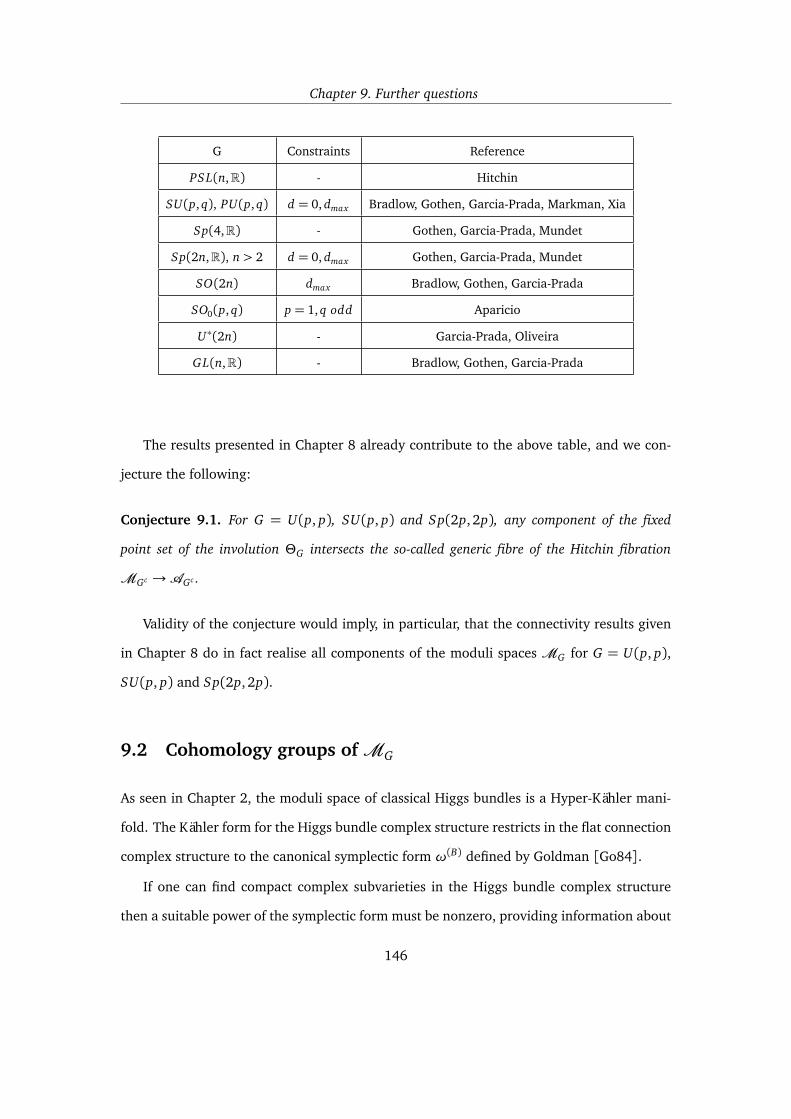
Chapter 9. Further questions
G Constraints Reference
PSL(n,R) - Hitchin
SU(p, q), PU(p, q) d = 0, dmax Bradlow, Gothen, Garcia-Prada, Markman, Xia
Sp(4,R) - Gothen, Garcia-Prada, Mundet
Sp(2n,R), n> 2 d = 0, dmax Gothen, Garcia-Prada, Mundet
SO(2n) dmax Bradlow, Gothen, Garcia-Prada
SO0(p, q) p = 1, q odd Aparicio
U∗(2n) - Garcia-Prada, Oliveira
GL(n,R) - Bradlow, Gothen, Garcia-Prada
The results presented in Chapter 8 already contribute to the above table, and we con-
jecture the following:
Conjecture 9.1. For G = U(p, p), SU(p, p) and Sp(2p, 2p), any component of the fixed
point set of the involution ΘG intersects the so-called generic fibre of the Hitchin fibration
MGc →AGc .
Validity of the conjecture would imply, in particular, that the connectivity results given
in Chapter 8 do in fact realise all components of the moduli spaces MG for G = U(p, p),
SU(p, p) and Sp(2p, 2p).
9.2 Cohomology groups ofMG
As seen in Chapter 2, the moduli space of classical Higgs bundles is a Hyper-Kähler mani-
fold. The Kähler form for the Higgs bundle complex structure restricts in the flat connection
complex structure to the canonical symplectic form ω(B) defined by Goldman [Go84].
If one can find compact complex subvarieties in the Higgs bundle complex structure
then a suitable power of the symplectic form must be nonzero, providing information about
146
9.3. Spectral data for other real forms
the corresponding space of representations. In particular, a Jacobian for U(p, p)-Higgs bun-
dles, as described in Chapter 6, or the moduli space of rank 2 vector bundles for Sp(2p, 2p)-
Higgs bundles, as described in Chapter 7, will give a lower bound for the non-vanishing of
cohomology groups.
9.3 Spectral data for other real forms
It would be very interesting to continue the research by extending the methods developed
in this thesis to other real forms G which appear to carry spectral data closely related to the
one studied in this thesis. In particular, the following groups present interesting scenarios:
• SU(p+ 1, 1)-Higgs bundles. From the description of SU(p, q)-Higgs bundles given in
Chapter 3, the spectral curve of an SU(p+ 1, 1)-Higgs bundle (E,Φ) lives in the total
space X of K with projection ρ : X → Σ, and has equation ηp(η2 + a1) = 0 for η the
tautological section of ρ∗K and a1 ∈ H0(Σ, K2). Following the ideas of Chapter 7,
we denote by S the curve given by a component of det(ρ∗Φ− η), whose equation is
η2+ a1 = 0.
One could try to follow the methods in [Xia03] to understand SU(p + 1,1)-Higgs
bundles via U(1, 1)-Higgs bundles (E1 := V/Vγ,Φ1 = (β1,γ1)) with additional data
obtained from the kernel Vγ of γ. For this, one may need to consider the set of vector
bundles
H pd := F : rkF = p , degF = d < 0 , degF ′ ≤ 0 for all F ′ ⊂ F.
Note that, by stability, Vγ ∈ Hp
d . In the case of p = 2, and degVγ = −1, one can see
that starting with a U(1,1)-Higgs bundle, the map β1 can generically be lifted to β
147
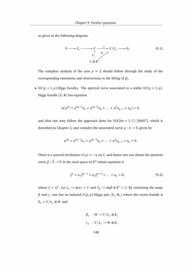
Chapter 9. Further questions
as given in the following diagram:
0 // Vγ // V π // V/Vγ // 0,
L⊗ K∗
β
OOβ1
::(9.1)
The complete analysis of the case p = 2 should follow through the study of the
corresponding extensions and obstructions to the lifting of β1.
• SU(p + 1, p)-Higgs bundles. The spectral curve associated to a stable SU(p + 1, p)-
Higgs bundle (E,Φ) has equation
η(η2p +η2p−2a1+η2p−4a2+ . . .+η2ap−1+ ap) = 0,
and thus one may follow the approach done for SO(2m + 1,C) [Hit07], which is
described in Chapter 2, and consider the associated curve ρ : S→ Σ given by
η2p +η2p−2a1+η2p−4a2+ . . .+η2ap−1+ ap = 0.
There is a natural involution σ(η) =−η on S, and hence one can obtain the quotient
curve ρ : S→ Σ in the total space of K2 whose equation is
ξp + a1ξp−1+ a2ξ
p−2+ . . .+ ap = 0, (9.2)
where ξ = η2. Let Lγ := kerγ ⊂ V and Vβ := imβ ⊗ K∗ ⊂ V. By restricting the maps
β and γ, one has an induced U(p, p)-Higgs pair (E1,Φ1) where the vector bundle is
E1 = V/Lγ⊕W and
β1 : W → V/Lγ⊗ K ,
γ1 : V/Lγ→W ⊗ K .
148
9.3. Spectral data for other real forms
By stability degLγ < 0 and the pair (E1,Φ1) is stable. Recall that in the case of
SO(2m + 1,C)-Higgs bundles, one could recover the SO(2m + 1,C)-Higgs bundle
from a rank 2m symplectic Higgs bundle together with a 1-dimensional eigenspace.
By means of the spectral data defined in Chapter 6, one could expect to obtain in-
formation of the SU(p + 1, p)-Higgs bundle by considering a U(p, p)-Higgs bundle,
whose data is understood, and extending it to a SU(p+ 1, p)-Higgs bundle by taking
an appropriate extension
0 // Vγ // V // V/Vγ // 0,
W ⊗ K∗
β
OOβ1
::(9.3)
and studying the obstruction for β to be a lift of β1.
• SO(p+ 2, p)-Higgs bundles. Consider (E,Φ) an SO(p+ 2, p)-Higgs bundle as defined
in Chapter 3, and let Vγ and Vβ be the rank 2 vector bundles defined as
Vγ := kerγ⊂ V and Vβ := imβ ⊗ K∗ ⊂ V.
Although SO(q, p)-Higgs bundles were studied in [Ap09], not much has been said
about the particular case of q = p + 2. By restricting the maps β and γ, one has
two induced U(p, p)-Higgs pairs (Ei ,Φi), for i = 1, 2, where E1 := V/Vγ ⊕W and
E2 := Vβ ⊕W .
It is expected that considering the extensions of these particular U(p, p)-Higgs bun-
dles (Ei ,Φi) by the rank 2 vector bundle Vγ, one could recover SO(p + 2, p)-Higgs
bundles. Although stability of an SO(p+ 2, p)-Higgs bundle does not imply directly
stability of the vector bundle Vγ, additional conditions could be set in order for the
149

Chapter 9. Further questions
implication to hold. In particular, understanding the low rank cases would provide
useful understanding of the corresponding space of surface group representations.
150
Bibliography
[AG06] J.E. Andersen, J. Grove, Automorphism fixed points in the moduli space of semi-
stable bundles, Q J Math 57 1 (2006) 1-35.
[Ap09] M. Aparicio Arroyo, The Geometry of SO(p, q)-Higgs Bundles, Ph.D. Thesis, Univer-
sidad de Salamanca (2009).
[ApG-P10] M. Aparicio Arroyo, O. García-Prada, Higgs bundles for the lorentz group,
arXiv:1004.0318 (2010).
[A89] H. Aslaksen, SO(2) invariants of a set of 2× 2 matrices MATH. SCAND. 65 (1989),
59-66
[AB68] M.F. Atiyah, R. Bott, A Lefschetz Fixed Point Formula for Elliptic Complexes: II. Ap-
plications, Ann. Math. 88, 3 (1968), 451-491.
[BNR] A. Beauville, M.S. Narasimhan and S. Ramanan, Spectral curves and the generalised
theta divisor, J. reine angew. Math. 398 (1989), 169-179.
[BiGo08] I. Biswas, T.L. Gómez, Connections and Higgs fields on a principal bundle, Ann.
Global Anal. Geom. 33, 1 (2008), 19-46.
[BG-PG03] S. Bradlow, O. García-Prada, P.G. Gothen, Surface group representations and
U(p, q)-bundles, J. Diff. Geom. 64 (2003), 111-170.
151

Bibliography
[BG-PG04] S. Bradlow, O. García-Prada, P.G. Gothen, Representations of surface groups in
the general linear group, arXiv:0401.064 (2004)
[BG-PG06] S. Bradlow, O. García-Prada, P.G. Gothen, Maximal surface group representa-
tions in isometry groups of classical Hermitian symmetric spaces, Geom. Dedicata 122
(2006), 185-213.
[BG-PG11] S. Bradlow, O. García-Prada, P.G. Gothen, Deformations of maximal representa-
tions in Sp(4,R), Quart. J. Math. 00 (2011), 1-49.
[BW12] S. Bradlow, G. Wilkin, Morse theory, Higgs fields, and Yang-Mills-Higgs functionals,
J. Fixed Point Theory Appl. 17 (2007) 1-32.
[BILW05] M. Burger, A. Iozzi, F. Labourie, A. Wienhard, Maximal representations of surface
groups: Symplectic Anosov structures, Pure Appl. Math. Q. 1 (2005).
[Ca50] H. Cartan, La transgression dans un group de Lie et dans un espace fibre principle,
Colloque de Topologie, Bruxelles (1950), 57-71.
[Ch50] C. Chevalley, The Betti numbers of the exceptional simple Lie groups, Proceedings of
the International Congress of Mathematicians, U (1950), 21-24.
[CG93] S. Choi, W.M. Goldman, Convex real projective structures on closed surfaces are
closed, Proc. Amer. Math. Soc. 118 (1993), 657-661.
[CG97] S. Choi, W.M. Goldman, The classification of real projective structures on compact
surfaces, Bull. Amer. Math. Soc., t. 34, 2 (1997), 161-171.
[Cop04] J. Copeland, A special subgroup of the surface braid group, arXiv:0409.461 (2004).
[Cop05] J. Copeland, Monodromy of the Hitchin map over hyperelliptic curves, IMRN
(2005), 1743-1785.
152

Bibliography
[Cor88] K. Corlette, Flat G-bundles with canonical metrics, J. Differential Geom. 28 (1988),
361-382.
[Do95] R. Donagi, Spectral Covers, MSRI Series, 28 (1995).
[DoMa96] R. Donagi, E. Markman, Spectral covers, algebraically completely integrable,
Hamiltonian systems, and moduli of bundles, Integrable Systems and Quantum Groups,
Montecatini Terme (1993).
[DoPa12] R. Donagi, T. Pantev, Langlands duality for Hitchin systems, Invent. math. (2012).
[D87] S.K. Donaldson, Twisted harmonic maps and the self-duality equations, Proc. London
Math. Soc. 55, 3 (1987), 127-131.
[FS03] J. Fuchs, C. Schweigert, Symmetries, Lie Algebras and Representations: A Graduate
Course for Physicists, Cambridge Monographs on Mathematical Physics, Camb. Univ.
Press (2003).
[G-PGM08] O. García-Prada, P.B. Gothen, I. Mundet i Riera, Higgs bundles and surface group
representations in the real symplectic group, arXiv:0809.0576v3 (2008).
[G-PGM09] O. García-Prada, P.B. Gothen, I. Mundet i Riera, The Hitchin-Kobayashi corre-
spondence, Higgs pairs and surface group representations, arXiv:0909.4487 (2009).
[G-PO10] O. García-Prada, A. Oliveira, Higgs bundles for the non-compact dual of the unitary
group, arXiv:1004.0245v2 (2010).
[G-P-Talk06] O. García-Prada, Involutions of the moduli space of SL(n,C)-Higgs bundles and
real forms, talk at the School (and workshop) on vector bundles and low codimensional
subvarieties, Trento (2006).
[Go84] W.M. Goldman, The symplectic nature of fundamental groups of surfaces, Adv. in
Math. 54 (1984) 200-225.
153
Bibliography
[Go88] W. M. Goldman, Topological components of spaces of representations, Invent. Math.
93 (1988), 557-607.
[G95] P.B. Gothen, The topology of Higgs bundle moduli spaces, Ph.D. thesis, Mathematics
Institute, University of Warwick (1995).
[G01] P.B. Gothen, Components of spaces of representations and stable triples, Topology 40,
4 (2001), 823-850.
[GO12] P.B. Gothen and A. Oliveira, The singular fibre of the Hitchin map, Int. Math. Res.
Notices, (2012).
[GK99] R. Gow, A. Kleshchev, Connections between the Representations of the Symmetric
Group and the Symplectic Group in Characteristic 2, Journal of Algebra, 221 (1999),
60-89.
[HT03] T. Hausel, and M. Thaddeus, Mirror symmetry, Langlands duality, and the Hitchin
system, Invent. Math. 153 (2003) 197-229 .
[Hit87] N.J. Hitchin, The self-duality equations on a Riemann surface, Proc. LMS 55, 3
(1987), 59-126.
[Hit87a] N.J. Hitchin, Stable bundles and integrable systems, Duke Math. J. 54, 1 (1987),
91-114.
[Hit92] N.J. Hitchin, Lie Groups and Teichmüller Space, Topology 31, 3 (1992), 449-473.
[Hit07] N.J. Hitchin, Langlands duality and G2 spectral curves, Q.J. Math., 58 (2007), 319-
344.
[He01] S. Helgason, Differential geometry, Lie groups, and symmetric spaces, Graduate Stud-
ies in Mathematics, AMS 34 (2001).
154

Bibliography
[J51] N. Jacobson, Completely reducible Lie algebras of linear transformations, Proceedings
of the American Mathematical Society, 2 (1951), 105-133.
[KW07] A. Kapustin, E. Witten, Electric-magnetic duality and the geometric Langlands pro-
gram. Commun. Number Theory Phys. 1 1 (2007) 1-236.
[Kn02] A.W. Knapp, Lie groups beyond an introduction, Progress in mathematics, 140
(2002).
[Kos59] B. Kostant, The principal three dimensional subgroup and the Betti numbers of a
complex simple Lie group, Amer. J. Math., 8, 1 (1959), 973-1032.
[Kos63] B. Kostant, Lie groups representations on polynomial rings, Amer. J. Math., 85
(1963), 327-404.
[La06] F. Labourie, Anosov flows, surface groups and curves in projective space, Invent. math.
165, (2006), 51-114.
[MX02] E. Markman, E.Z Xia, The moduli of flat PU(p, p)-structures with large Toledo in-
variants, Math. Z. 240 (2002), 95-109.
[Mor42] V.V. Morosov, On a nilpotent element of a semi-simple Lie algebra, Akademiia Nauk
SSSR (Doklady), 36 (1942), 83-86.
[N91] N. Nitsure, Moduli spaces of semistable pairs on a curve, Proc. London Mach. Sot. 62
(1991). 275-300.
[N86] N. Nitsure, Cohomology of the moduli space of parabolic vector bundles, Proc. Indian
Acad. Sci 95 (1986) 61-77.
[Ol10] A. Oliveira, Representations of surface groups in the projective general linear group,
Internat. J. Math (2010).
155

Bibliography
[OnVi] A.L. Onishchik, E.B. Vinberg, Lie groups and Lie algebras III: structure of Lie groups
and Lie algebras, Encyclopaedia of mathematical sciences: Lie groups and Lie algebras
Volume 3, Springer (1994).
[Ra75] A. Ramanathan, Stable principal bundles on a compact Riemann surface, Math. Ann.
213 (1975), 129-152.
[SW] A.A. Sagle, R.E. Walde, Introduction to Lie groups and Lie algebras, Pure and Applied
Mathematics, Academic Press 51 (1973).
[Sch11] L.P. Schaposnik, Monodromy of the SL2 Hitchin fibration, ArXiv:1111.2550v1 (to
appear in IJM, 2013) (2011)
[S88] C.T. Simpson, Constructing variations of Hodge structure using Yang-Mills theory and
applications to uniformisation, Journal of the AMS 1 (1988). 867-918.
[S92] C.T. Simpson, Higgs bundles and local systems, Publ. Math. I.H.E.S. 75 (1992), 5-95.
[W10] K. Walker, Quotient groups of the fundamental groups of certain strata of the moduli
space of quadratic differentials, Geometry and Topology, 14 (2010), 1129-1164.
[Xia97] E.Z. Xia, Components of Hom(π1, PGL(2,R)), Topology 36 (1997), 481-499.
[Xia00] E.Z. Xia, The moduli of flat PU(2,1) structures over Riemann surfaces, Pacific Jour-
nal of Mathematics 195 (2000), 231-256 .
[Xia03] E.Z. Xia, The moduli of flat U(p, 1) structures on Riemann surfaces, Geometriae
Dedicata 97 (2003), 33-43.
156


