SPEECH RECOGNITION USING
TIME DOMAIN FEATURES FROM PHASE SPACE
RECONSTRUCTIONS
by
Jinjin Ye, B.S.
A THESIS
SUBMITTED TO THE FACULTY OF THE GRADUATE SCHOOL
IN PARTIAL FULFILLMENT OF THE REQUIREMENTS
for the degree of
MASTER OF SCIENCE
Field of Electrical and Computer Engineering
Marquette University
Milwaukee, Wisconsin
May 2004
ii
Abstract
A speech recognition system implements the task of automatically transcribing speech
into text. As computer power has advanced and sophisticated tools have become
available, there has been significant progress in this field. But a huge gap still exists
between the performance of the Automatic Speech Recognition (ASR) systems and
human listeners. In this thesis, a novel signal analysis technique using Reconstructed
Phase Spaces (RPS) is presented for speech recognition. The most widely used
techniques for acoustic modeling are currently derived from frequency domain feature
extraction. The reconstructed phase space modeling technique taken from dynamical
systems methods addresses the acoustic modeling problem in the time domain instead.
Such a method has the potential of capturing nonlinear information usually ignored by
the traditional linear human speech production model. The features from this time
domain approach can be used for speech recognition when combined with statistical
modeling techniques such as Hidden Markov Models (HMM) and Gaussian Mixture
Models (GMM). Issues associated with this RPS approach are discussed, and
experiments are done using the TIMIT database. Most of this work focuses on isolated
phoneme classification, with some extended work presented on continuous speech
recognition. The direct statistical modeling of RPS can be used for the isolated phoneme
recognition. The Singular Value Decomposition (SVD) is used to extract frame-based
features from RPS, and can be applied to both isolated phoneme recognition and
continuous speech recognition.

iii
Acknowledgments
I am indebted to many people who have contributed to this research. I especially
thank my advisor, Dr. Michael Johnson, for his guidance, great insights and creative
thoughts on my work. His mentoring and support through my years at Marquette have
made this work possible. I thank Dr. Richard Povinelli, for his numerous ideas,
discussions, and collaboration on this research. I also thank Dr. Edwin Yaz for serving on
my thesis committee, reviewing the manuscript, and giving suggestions. In addition, I
thank my colleagues, Felice, Xiaolin, Andy, Kevin, Pat, Franck, and Emad, for their
discussions and contributions to this work. I thank other members of the Speech and
Signal Processing Laboratory, the KID Laboratory, and the ACT Laboratory for their
help and friendship.
I thank my family for their love, encouragement, and constant support of my
educational endeavors.
Finally, I thank National Science Foundation for funding this research.

iv
Table of Contents
LIST OF FIGURES ...................................................................................................... VII
LIST OF TABLES .......................................................................................................... IX
1. INTRODUCTION....................................................................................................... 1
1.1 OVERVIEW OF SPEECH RECOGNITION ...................................................................... 1
1.1.1 Historical Background.................................................................................... 1
1.1.2 Automatic Speech Recognition ....................................................................... 2
1.1.3 Acoustic Feature Representation.................................................................... 3
1.2 NONLINEAR SIGNAL PROCESSING TECHNIQUES....................................................... 4
1.3 MOTIVATION OF RESEARCH..................................................................................... 6
1.4 THESIS ORGANIZATION............................................................................................ 6
2. SPEECH PROCESSING AND RECOGNITION ................................................... 7
2.1 ACOUSTIC MODELING.............................................................................................. 7
2.1.1 Cepstral Processing ........................................................................................ 8
2.1.2 Common Features........................................................................................... 9
2.1.3 Feature Transformation................................................................................ 12
2.1.4 Variability in Speech..................................................................................... 12
2.2 GAUSSIAN MIXTURE MODELS ............................................................................... 13
2.3 HIDDEN MARKOV MODELS.................................................................................... 15
2.3.1 Definition ...................................................................................................... 16
2.3.2 Practical Issues............................................................................................. 18
2.4 ISOLATED VS. CONTINUOUS SPEECH RECOGNITION............................................... 19

v
2.5 SUMMARY.............................................................................................................. 20
3. RECONSTRUCTED PHASE SPACES FOR SPEECH RECOGNITION......... 21
3.1 FUNDAMENTAL THEORY........................................................................................ 21
3.2 DIRECT STATISTICAL MODELING OF RPS .............................................................. 23
3.2.1 Bin-based Distribution Modeling ................................................................. 24
3.2.2 GMM-based Distribution Modeling ............................................................. 25
3.3 CLASSIFIER ............................................................................................................ 26
3.4 DATASETS AND SOFTWARE.................................................................................... 26
3.5 CHOOSING LAG AND DIMENSION ........................................................................... 28
3.6 ISSUES OF SPEECH SIGNAL VARIABILITY USING RPS BASED METHOD.................. 43
3.6.1 Effect of Principal Component Analysis on RPS .......................................... 43
3.6.2 Effect of Vowel Pitch Variability .................................................................. 47
3.6.3 Effect of Speaker Variability......................................................................... 50
3.7 SUMMARY.............................................................................................................. 53
4. FRAME-BASED FEATURES FROM RECONSTRUCTED PHASE SPACES 54
4.1 WHY USE FRAME-BASED FEATURES ...................................................................... 54
4.2 FRAME-BASED FEATURES FROM RPS .................................................................... 55
4.3 SVD DERIVED FEATURES...................................................................................... 55
4.3.1 Global SVD Derived Features ...................................................................... 55
4.3.2 Regional SVD Derived Features................................................................... 57
4.4 IMPLEMENTATION FOR SPEECH RECOGNITION TASKS............................................ 58
4.5 SUMMARY.............................................................................................................. 59
vi
5. EXPERIMENTAL SETUP AND RESULTS ......................................................... 60
5.1 RPS ISOLATED PHONEME CLASSIFICATION ........................................................... 60
5.1.1 Baselines ....................................................................................................... 60
5.1.2 Experiments using Frame-Based SVD Derived Features............................. 61
5.1.3 Experiments using Combined Features ........................................................ 64
5.2 RPS CONTINUOUS SPEECH RECOGNITION ............................................................. 65
5.3 DISCUSSION ........................................................................................................... 66
6. CONCLUSIONS AND FUTURE WORK.............................................................. 68
6.1 CONCLUSIONS........................................................................................................ 68
6.2 FUTURE WORK ...................................................................................................... 69
7. REFERENCES.......................................................................................................... 71

vii
List of Figures
Figure 1 – Basic architecture of speech recognition system............................................... 2
Figure 2 – Source-filter model for speech signals .............................................................. 4
Figure 3 – Triangular filters used in the MFCC computation ............................................ 9
Figure 4 – Block diagram of feature extraction for a typical speech recognition system 11
Figure 5 – An HMM structure .......................................................................................... 16
Figure 6 – Examples of three dimensional reconstructed phase spaces ........................... 23
Figure 7 – Dividing RPS into bins for PMF estimation ................................................... 25
Figure 8 – Histogram of first minimum of automutual function for all phoneme............ 31
Figure 9 – Histogram of first minimum of automutual function for vowels .................... 31
Figure 10 – Histogram of first minimum of automutual function for affricates and
fricatives ........................................................................................................ 32
Figure 11 – Histogram of first minimum of automutual function for semivowels and
glides.............................................................................................................. 32
Figure 12 – Histogram of first minimum of automutual function for nasals.................... 33
Figure 13 – Histogram of first minimum of automutual function for stops ..................... 33
Figure 14 – Histogram of dimension by FNN approach (Set 1) for all phonemes........... 35
Figure 15 – Histogram of dimension by FNN approach (Set 1) for vowels..................... 35
Figure 16 – Histogram of dimension by FNN approach (Set 1) for affricates and fricatives
....................................................................................................................... 36
Figure 17 – Histogram of dimension by FNN approach (Set 1) for semivowels and glides
....................................................................................................................... 36
Figure 18 – Histogram of dimension by FNN approach (Set 1) for nasals ...................... 37

viii
Figure 19 – Histogram of dimension by FNN approach (Set 1) for stops........................ 37
Figure 20 – Histogram of dimension by FNN approach (Set 2) for all phonemes........... 38
Figure 21 – Histogram of dimension by FNN approach (Set 2) for vowels..................... 38
Figure 22 – Histogram of dimension by FNN approach (Set 2) for affricates and fricatives
....................................................................................................................... 39
Figure 23 – Histogram of dimension by FNN approach (Set 2) for semivowels and glides
....................................................................................................................... 39
Figure 24 – Histogram of dimension by FNN approach (Set 2) for nasals ...................... 40
Figure 25 – Histogram of dimension by FNN approach (Set 2) for stops........................ 40
Figure 26 – TIMIT Accuracy vs. dimension at lag of 6 ................................................... 41
Figure 27 – TIMIT Accuracy vs. lag at dimension of 11 ................................................. 42
Figure 28 – The classification accuracy vs. number of speakers...................................... 52

ix
List of Tables
Table 1 – Results of speaker-dependent 48 phonemes using PCA on RPS...................... 46
Table 2 – Results on speaker-independent fricatives using PCA on RPS ........................ 46
Table 3 – Results on speaker-independent vowels using PCA on RPS............................ 47
Table 4 – Results on speaker-independent nasals using PCA on RPS ............................. 47
Table 5 – Range of τ ′ given τ and 0f .............................................................................. 50
Table 6 – Vowel phoneme variable lag classification results for lag of 6........................ 50
Table 7 – Vowel phoneme variable lag classification results for lag of 12...................... 50
Table 8 – Classification results of fricatives on various numbers of speakers ................. 51
Table 9 – Classification results of vowels on various numbers of speakers..................... 52
Table 10 – Classification results of nasals on various numbers of speakers .................... 52
Table 11 – Baseline phoneme accuracy............................................................................ 61
Table 12 – Phoneme accuracy on SVD feature (128 mix) ............................................... 62
Table 13 – Phoneme accuracy on SVD feature using nonlinear operator (128 mix) ....... 62
Table 14 – Phoneme accuracy on regional SVD feature (128 mix) ................................. 63
Table 15 – Phoneme accuracy on combined features (MFCC+SVD).............................. 64
Table 16 – Phoneme accuracy on combined features (MFCC+regional SVD)................ 64
Table 17 – CSR results (3-state monophone HMM, 8 mix, bigram)................................ 65

1
1. Introduction
1.1 Overview of Speech Recognition
1.1.1 Historical Background
Speech recognition has a history of more than 50 years. With the emerging of
powerful computers and advanced algorithms, speech recognition has undergone a great
amount of progress over the last 25 years. The earliest attempts to build systems for
automatic speech recognition (ASR) were made in 1950s based on acoustic phonetics.
These systems relied on spectral measurements, using spectrum analysis and pattern
matching to make recognition decisions, on tasks such as vowel recognition [1]. Filter
bank analysis was also utilized in some systems to provide spectral information. In the
1960s, several basic ideas in speech recognition emerged. Zero-crossing analysis and
speech segmentation were used, and dynamic time aligning and tracking ideas were
proposed [2]. In the 1970s, speech recognition research achieved major milestones. Tasks
such as isolated word recognition became possible using Dynamic Time Warping
(DTW). Linear Predictive Coding (LPC) was extended from speech coding to speech
recognition systems based on LPC spectral parameters. IBM initiated the effort of large
vocabulary speech recognition in the 70s [3], which turned out to be highly successful
and had a great impact in speech recognition research. Also, AT&T Bell Labs began
making truly speaker-independent speech recognition systems by studying clustering
algorithms for creating speaker-independent patterns [4]. In the 1980s, connected word
recognition systems were devised based on algorithms that concatenated isolated words
for recognition. The most important direction was a transition of approaches from
template-based to statistical modeling – especially the Hidden Markov Model (HMM)

2
approach [5]. HMMs were not widely used in speech application until the mid-1980s.
From then on, almost all speech research has involved using the HMM technique. In the
late 1980s, neural networks were also introduced to problems in speech recognition as a
signal classification technique. Recent focus is on large vocabulary, continuous speech
recognition systems. Major contributors in this direction are Defense Advanced Research
Projects Agency (DARPA), Carnegie Mellon University (the SPHINX system), BBN,
Lincoln Labs, SRI, MIT (the SUMMIT system), AT&T Bell Labs and IBM.
1.1.2 Automatic Speech Recognition
A source filter model is often used to describe the speech production mechanism.
This model has been successful exploited in applications such as speech coding, synthesis
and recognition for many years [6]. A typical automatic speech recognition system
consists of the basic components shown in Figure 1.
Voice Signal Processing
Decoder
Adaptation
Acoustic
Models
Application
LanguageM
odels
Voice Signal Processing
Decoder
Adaptation
Acoustic
Models
Application
LanguageM
odels
Figure 1 – Basic architecture of speech recognition system

3
Acoustic models include knowledge about phonetics, acoustics, environmental
variability, and gender and speaker variabilities, etc, while language models include
knowledge of word possibilities, syntax, and semantics information. The speech signal is
processed in the signal-processing module that extracts effective feature vectors for the
decoder. The decoder uses both acoustic and language models to generate the word
sequence that has the maximum posterior probability for the input feature vectors. Both
acoustic model and language model can provide information for the adaptation
component in order to obtain improved performance over time. In our work, we focus on
the signal-processing module, to study the features from time domain analysis technique.
This is a dramatically different approach from the existing signal processing method for
speech recognition applications.
1.1.3 Acoustic Feature Representation
Traditional acoustic features are derived from the decomposition of the speech signal
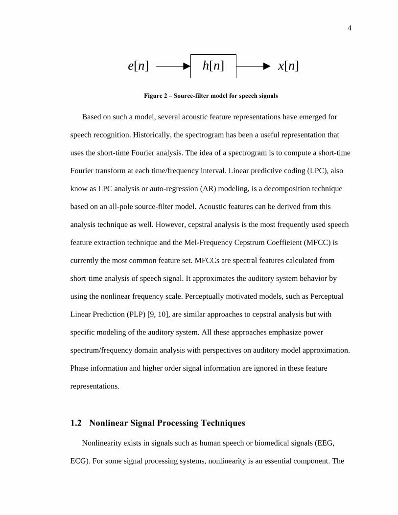
as a source through a linear time varying filter [3, 7, 8]. Figure 2 shows this model, where
is the excitation from vocal folds, is the vocal tract filter and [ ]e n [ ]h n [ ]x n is the output
speech signal. Current state-of-the-art acoustic feature representation is based on such a
speech production model. Because of the time varying nature of speech signals, features
are calculated on frame-by-frame basis assuming speech signal stationarity within each
frame. Speech recognizers estimate the filter characteristics and usually ignore the
excitation because the information for speech recognition mostly depends on vocal tract
characteristics. Thus, separation between source and filter is one of the important tasks in
speech processing.
4
e[n] h[n] x[n]e[n] h[n] x[n]
Figure 2 – Source-filter model for speech signals
Based on such a model, several acoustic feature representations have emerged for
speech recognition. Historically, the spectrogram has been a useful representation that
uses the short-time Fourier analysis. The idea of a spectrogram is to compute a short-time
Fourier transform at each time/frequency interval. Linear predictive coding (LPC), also
know as LPC analysis or auto-regression (AR) modeling, is a decomposition technique
based on an all-pole source-filter model. Acoustic features can be derived from this
analysis technique as well. However, cepstral analysis is the most frequently used speech
feature extraction technique and the Mel-Frequency Cepstrum Coeffieient (MFCC) is
currently the most common feature set. MFCCs are spectral features calculated from
short-time analysis of speech signal. It approximates the auditory system behavior by
using the nonlinear frequency scale. Perceptually motivated models, such as Perceptual
Linear Prediction (PLP) [9, 10], are similar approaches to cepstral analysis but with
specific modeling of the auditory system. All these approaches emphasize power
spectrum/frequency domain analysis with perspectives on auditory model approximation.
Phase information and higher order signal information are ignored in these feature
representations.
1.2 Nonlinear Signal Processing Techniques
Nonlinearity exists in signals such as human speech or biomedical signals (EEG,
ECG). For some signal processing systems, nonlinearity is an essential component. The

5
use of nonlinear techniques in speech processing is a rapidly growing area of research.
There are large variety of methods found in the literature, including linearization as in the
field of adaptive filtering [11], and various forms of oscillators and nonlinear predictors
[12]. Nonlinear predictors are part of the more general class of nonlinear autoregressive
models. Various approximations for nonlinear autoregressive models have been
proposed, in two main categories: parametric and nonparametric methods. Parametric
methods are exemplified by polynomial approximation, locally linear models [13], and
state dependent models, as well as neural networks. Nonparametric methods include
various nearest neighbor methods [14] and kernel-density estimates. Another class of
nonlinear speech processing methods includes models and digital signal processing
algorithms proposed to analyze nonlinear phenomena of the fluid dynamics type in the
speech airflow during speech production [15]. The investigation of the speech airflow
nonlinearities can result in development of nonlinear signal processing systems suitable
to extract related information of such phenomena. Recent work includes speech
resonances modeling using AM-FM model [16], measuring the degree of turbulence in
speech sounds using fractals [17], and applying nonlinear speech features to speech
recognition [17, 18].
Our work in speech recognition focuses on integrating techniques from chaos and
dynamical systems theory to the task of speech recognition. The work utilizes
Reconstructed Phase Spaces (RPS) from dynamical systems theory [19-21] for signal
analysis and feature extraction. A detailed discussion of RPSs for speech recognition can
be found in Chapter 3.

6
1.3 Motivation of Research
As discussed previously, current speech recognition systems typically use frequency
domain features, obtained via a frame-based spectral analysis of the speech signal. Such
frequency domain approaches are constrained by linearity assumptions incurred by the
source-filter model of speech production. Research has suggested that there is evidence
of nonlinear behavior in speech signals [22, 23]. The RPS representation is capable of
preserving the nonlinear dynamics of the signal. This method addresses the problem in
the time domain instead of the frequency domain so that nonlinear information can be
captured. The application of RPSs for speech recognition is a new path of research and is
still in its very early stages. The potential of this method for speech recognition motivates
the work presented in the thesis. In pursuit of this direction, we have done experiments
using RPSs for speech recognition tasks such as isolated phoneme classification and
continuous speech recognition. Because acoustic features are being investigated and
compared, the evaluation is primarily based on the isolated phoneme classification task.
1.4 Thesis Organization
The thesis is organized as follows. Chapter 2 gives an overview of conventional
speech processing and recognition methods. Chapter 3 introduces the RPS approach for
speech recognition and discusses various issues associated with this technique. Chapter 4
focuses on developing various frame-based features from RPSs and the implementation
of speech recognition tasks using these features. Chapter 5 describes experiments and
presents experimental results. The conclusions and future work are detailed in Chapter 6.

7
2. Speech Processing and Recognition 2.1 Acoustic Modeling
If an acoustic observation sequence is denoted as 1 2... nx x x=X and the word sequence
is , then the maximum posterior probability is computed as 1 2... mw w w=W ( | )P W X
( ) ( | )( | )( )
P PPP
=W X WW X
X. (2.1)
The estimated word sequence is therefore W
( ) ( | )ˆ arg max ( | ) arg max arg max ( ) ( | ),( )w w w
P PP PP
= = =W X WW W X W X
XP W (2.2)
since the acoustic observation is fixed. X
The acoustic model and the language model are the two underlying
challenges to building a speech recognition system. should take into account
phonetic variations, speaker variations, and environmental variations. The process of
finding the best word sequence given the input speech signal is a difficult pattern
classification problem [24], due to the complex and nonstationary nature of the task.
( | )P X W ( )P W
( | )P X W
W X
The Hidden Markov Model (HMM) is the foundation for acoustic phonetic modeling.
It incorporates segmentation, time warping, pattern matching, and context knowledge in a
unified way. It has become the prevailing choice of statistical model for continuous
speech recognition tasks. Section 2.3 will summarize the HMM in detail. As mentioned
before, the work of the thesis concentrates on acoustic models of speech. Thus, the
speech processing and recognition discussed in this chapter involve no language models.
8
2.1.1 Cepstral Processing
The cepstrum is obtained by taking the inverse Fourier transform of the log spectrum.
There are two types of cepstrums: complex cepstrum and real cepstrum. Let [ ]x n denote
the original signal. The complex cepstrum is defined as:
(2.3) 1ˆ[ ] {log( { [ ]})},x n FT FT x n−=
and the real cepstrum is defined as:
(2.4) 1[ ] {log(| { [ ]} |)},c n FT FT x n−=
where FT denotes Fourier transform.
The cepstrum is a homomorphic transformation [6] that converts a convolution
[ ] [ ]* [ ]x n e n h n= (2.5)
into a sum in the cepstrum domain
ˆˆ ˆ[ ] [ ] [ ].x n e n h n= + (2.6)
This type of transformation allows the separation of the source from the filter. In the
cepstrum domain, the excitation and filter are split apart, so we can
approximately recover both and from
ˆ[ ]e n ˆ[ ]h n
[ ]e n [ ]h n ˆ[ ]x n by homomorphic filtering.
The term quefrency is used to represent the independent variable n in and is
measured in time units. The log operation in Equation (2.4) combined with two Fourier
transforms separates the excitation and vocal tract spectrum in the cepstrum domain such
that the vocal tract information is in the low quefrency and the excitation is in the high
quefrency.
[ ]c n
In addition, the complex cepstrum can be obtained from the LPC coefficients by a
recursive method [6]. Empirical study has shown that a finite number of cepstrum

9
coefficients is sufficient for speech recognition, usually in the range of 12-20 depending
on the sampling rate and whether or not frequency warping is used. Cepstral coefficients
tend to be uncorrelated, which is very useful for building machine learning models for
speech recognition.
2.1.2 Common Features
Mel-Frequency Cepstrum Coefficients (MFCCs) are related to the real cepstrum of a
windowed short-time signal derived from the FFT of that signal. It differs from the real
cepstrum in that a nonlinear frequency scale, the Mel-Frequency scale [25], is used.
Because this scale is based on the human auditory system, it is beneficial to use such a
scale for speech recognition tasks.
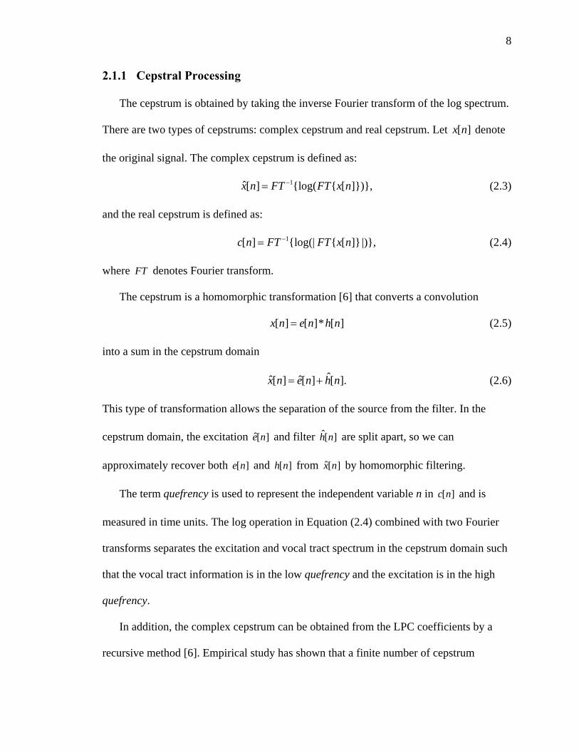
MFCCs are computed by using filterbanks. The filterbanks consists of triangular
filters as shown in Figure 3. Such filters compute the spectrum around each center
frequency with increasing bandwidths.
……
f
|DFT|
……
f
|DFT|
Figure 3 – Triangular filters used in the MFCC computation
10
After defining the lowest and highest frequencies of the filterbank and the number of
filters, the boundary frequencies of filterbank are uniformly spaced in the Mel scale,
which is given by:
1127 ln(1 ).700
fm = + (2.7)
The log-energy at the output of each filter is computed afterwards. The mel-frequency
cepstrum is the Discrete Cosine Transform (DCT) of the filter energy outputs:
(2.8) 1
0[ ] [ ]cos( ( 1/ 2) / ) 0 ,
M
mc n S m n m M n Mπ
−
=
= −∑ ≤ <
n
where is the log-energy at the output of each filter, and M is the number of filters,
which varies for different implementations from 24 to 40.
[ ]S m
Usually, only the first 12 cepstrum coefficients (excluding , the 0[0]c th coefficient)
are used. The advantage of computing MFCC by using filter energies is that they are
more robust to noise and spectral estimation errors. Although corresponds to the
energy measure, it is preferred to calculate log-energy separately for the framed speech
signal:
[0]c
(2.9) 2
1log [ ].
N
nE x
=
= ∑
The features outlined above don’t have temporal information. In order to incorporate
the ongoing changes over multiple frames, time derivatives are added to the basic feature
vector. The first and second derivatives of the feature are usually called Delta coefficients
and Delta-Delta coefficients respectively. The Delta coefficients are computed via a
linear regression formula:
11
1
2
1
( [ ] [ ])[ ]
2
k
ik
i
i c m i c m ic m
i
=
=
+ − −∆ =
∑
∑ (2.10)
where is the size of the regression window and is the MFCC coefficient. 2k +1 [ ]c m thm
The Delta-Delta coefficients are computed using linear regression of Delta features.
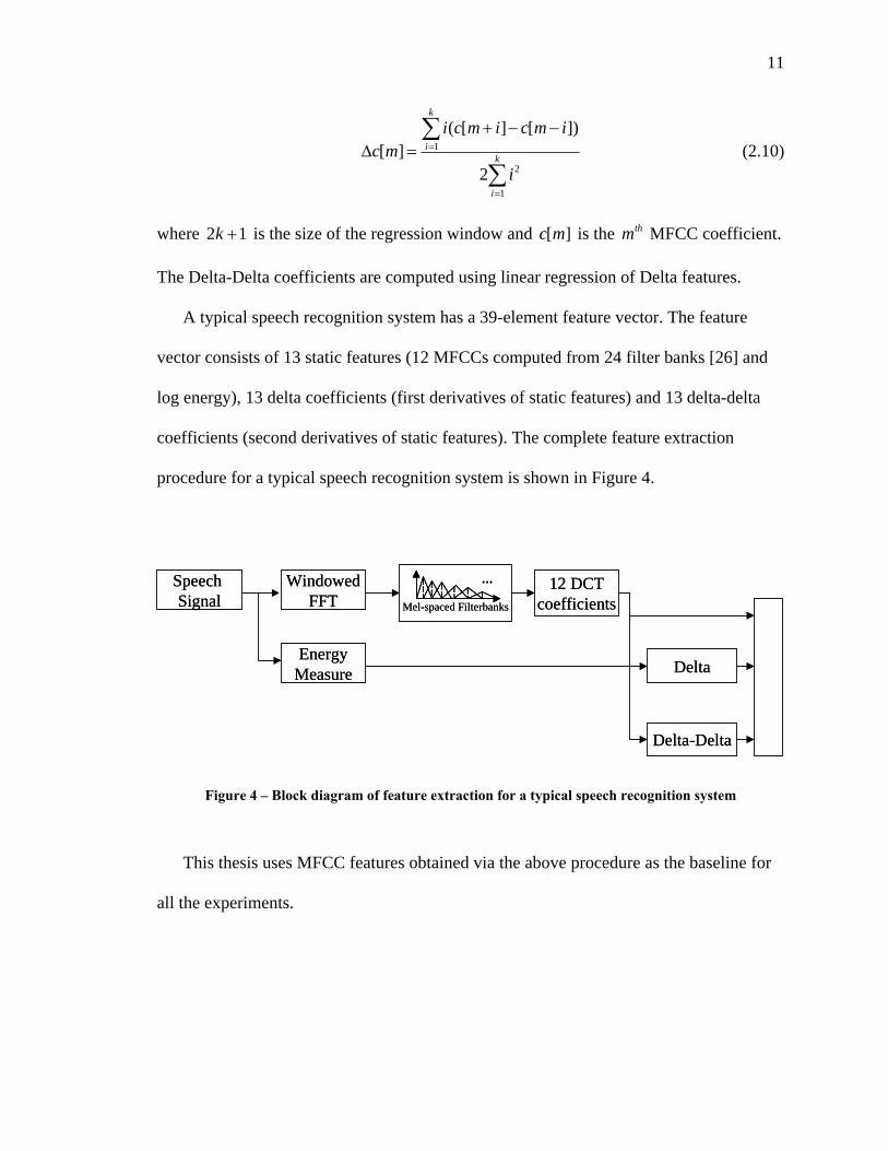
A typical speech recognition system has a 39-element feature vector. The feature
vector consists of 13 static features (12 MFCCs computed from 24 filter banks [26] and
log energy), 13 delta coefficients (first derivatives of static features) and 13 delta-delta
coefficients (second derivatives of static features). The complete feature extraction
procedure for a typical speech recognition system is shown in Figure 4.
Speech Signal Mel-spaced Filterbanks
…
EnergyMeasure
WindowedFFT
12 DCTcoefficients
Delta-Delta
Delta
Speech Signal Mel-spaced Filterbanks
……
EnergyMeasure
WindowedFFT
12 DCTcoefficients
Delta-Delta
Delta
Figure 4 – Block diagram of feature extraction for a typical speech recognition system
This thesis uses MFCC features obtained via the above procedure as the baseline for
all the experiments.
12
2.1.3 Feature Transformation
To cope with environmental noise, speaker variations and channel distortion, various
feature transformations can be utilized. By transforming the features that are most
effective for recognition, the recognition error rate can be further reduced. Sometimes, it
is also useful to reduce the dimension of the feature vector in order to lower the
computational cost. Principal Component Analysis (PCA) [24, 27] is such a
transformation, which is investigated on RPSs in Chapter 3.
The best criterion for selecting what feature sets to use should be based on reducing
the recognition error. It is usually hard to evaluate the feature sets systematically
according to this criterion. Linear Discriminant Analysis (LDA) [24] is a common
method based on criterion that addresses class separability by using within-class and
between-class scatter matrices. In a manner similar to PCA, LDA can reduce the
dimension of the original feature space too. Other feature processing techniques, such as
frequency warping for vocal tract length normalization (VTLN), have been used to
reduce interspeaker variability.
It is of interest to know that various feature transformation methods have limited
contribution to the reduction of recognition error, typically fewer than 10% on relative
error [7].
2.1.4 Variability in Speech
The current state-of-art speech recognition system still cannot beat human
performance in most tasks. It remains a challenge to build a recognition system that is
robust as to different speakers, different languages and speaking styles, and different
speaking environments. As accuracy and robustness are the most important measures of
13
speech recognition systems, variability in speech signals is a major factor that needs to be
addressed.
Variablity in pronunciation exists at the phonetic level as well as word and sentence
levels. The acoustic realization of a phoneme depends on its left and right context,
especially in fast speech and spontaneous speech conversation. In continuous speech
recognition, the same thing happens at the word and sentence levels. Also, interspeaker
variability affects the performance of speech recognition systems. This is due to the
differences in vocal tract length, physical characteristics, age, sex, dialect, health,
education, and talking style, etc. Finally, the variability in environment, especially in
noisy environments, affects the accuracy of speech recognizer. Environmental noise has
different types and may come from various sources such as input device, microphone,
A/D quantization noise, etc. Environmental variability remains one of the most severe
challenges facing today’s speech recognition system despite the progress made in recent
years.
2.2 Gaussian Mixture Models
Gaussian Mixture Models (GMM) are probability density models that comprise a
number of component Gaussian functions. These component functions are combined to
provide a multimodal density. They can be used to model almost any probability density
function (PDF) [28]. GMM is a parametric model and provides flexibility and precision
in modeling the underlying statistics of sample data. A GMM is defined as:
(2.11) ( ) ( ) ( )1 1
ˆ ˆ ; ,M M
m m m m mm m
p w p w= =
= =∑ ∑x x x µ ΣN ,
14
where M is the number of mixtures, ( ); ,m mx µ ΣN is a normal distribution with mean
mµ and covariance matrix , and is the mixture weight. As seen from the formula,
each mixture component is a Gaussian , and
mΣ mw
1mw =∑ guarantees that it is a valid
probability model. The Gaussian distribution is defined as:
( ) ( ) ( ) ( )1
1221; , 2 exp2
d T
m m m m m mπ −− −⎛ ⎞= − −⎜ ⎟⎝ ⎠
x µ Σ Σ x µ Σ x µN ,− (2.12)
where d is the dimension of feature space.
Expectation-Maximization (EM) [29, 30] is a well established maximum likelihood
algorithm for fitting the GMM model to a set of training data. It is guaranteed to find a
local maximum [29]. An iterative algorithm derived from EM that yields a maximum
likelihood estimate for the GMM parameters is given by:
( )
( )
' 1
1
,
T
m t tt
m T
m tt
p x x
p xµ =
=
=∑
∑ (2.13)
( )( ) ( )
( )
' 1
1
,
TT
m t t m t mt
m T
m tt
p x x x
p x
µ µ=
=
− −Σ =
∑
∑ (2.14)
( )
( )
' 1
1 1
.
T
m tt
m T M
m tt m
p xw
p x
=
= =
=∑
∑∑ (2.15)
15
EM requires a priori selection of model order, i.e. the number of components to be
incorporated into the model. The user may select a suitable number, roughly
corresponding to the number of distinct clusters in the feature space. For an unknown
distribution, the required number of mixtures is related to the underlying distribution of
the feature space. The classification accuracy tends toward an asymptote as the number of
mixtures increases provided there is sufficient training data. Too few mixtures can lead to
poor representations of feature distribution while too many mixture can have data
memorization problem because of overfitting of training data but decreased testing
performance. Selecting the appropriate number of mixtures is important to the
performance of the GMM model.
2.3 Hidden Markov Models
The Hidden Markov Model (HMM) is a very powerful statistical tool for acoustic
modeling in speech recognition and can be utilized for many other applications. It
incorporates parametric models, such as GMMs, and provides a unified pattern
classification of time varying data sequences via dynamic programming. The HMM has
become one of the most powerful statistical methods for modeling speech signals. It has
been widely used in various speech applications [3, 5, 6, 26, 31]. An HMM structure
diagram is illustrated in Figure 5.

16
a22 a33 a44
a24
a34a23a12 a45
a35a13
S1 S2 S3 S4 S5Start State End State
b2(•) b3(•) b4(•)
a22 a33 a44
a24
a34a23a12 a45
a35a13
S1 S2 S3 S4 S5Start State End State
b2(•) b3(•) b4(•)
Figure 5 – An HMM structure
2.3.1 Definition
An HMM is a Markov chain where the output observation is a random variable
generated according to an output probabilistic function associated with each state.
Formally, an HMM is defined by:
• , the state transition probability matrix, where is the probability of
taking a transition from state i to state j.
{ }ija=A ija
• , the set of state output probability distribution, where is the
probability of emitting when state i is entered.
{ ( )}i tb o=B ( )i tb o
to
• { }iπ=π , the initial state distribution.
Since , , and ija ( )i tb o iπ are all probabilities, they must satisfy the following properties:
0, ( ) 0, 0 ,ij i t ia b o all i jπ≥ ≥ ≥ ∀ (2.16)
1
1N
ijj
a=
=∑ (2.17)
( ) 1t
i to
b o∀
=∑ (2.18)

17
1
1N
ii
π=
=∑ (2.19)
where N is the total number of states. In the discrete state observation case, is
discrete probability mass function (PMF). It can be extended to the continuous case with
a continuous parametric probability density function (PDF). Conversely, a continuous
vector variable can be mapped to a discrete set using vector quantization [6]. A complete
HMM can now be defined as:
( )i tb o
( , , )λ = A B π (2.20)
where λ is the complete parameter set to represent the HMM.
Two formal assumptions characterize HMMs as used in speech recognition. The first-
order Markov assumption states that history has no influence on the Markov chain’s
future evolution if the present is specified. The output independence assumption states
that the present observation depends only on the current state and neither chain evolution
nor past observations influence it if the last chain transition is specified. These
assumptions can greatly reduce the number of parameters that need to be estimated as
well as the model complexity without significantly affecting the speech system
performance.
In order to apply HMM to speech applications, there are three basic problems that
need to be solved [5]:
1. The evaluation problem: Given a model λ and an observation sequence
, what is the probability 1 2( , ,..., )To o o=O ( | )P λO , i.e. the probability that the
model generates the observations?
18
2. The decoding problem: Given a model λ and an observation sequence
, what is the most likely state sequence in
the model that produces the observations?
1 2( , ,..., )To o o=O 1 2( , ,..., )Ts s s=S
3. The learning problem: Given a model λ and an observation sequence
, how to adjust the model parameter 1 2( , ,..., )To o o=O λ to maximize the
likelihood probability ( | )P λO ?
The implementation of the above three problems shares the same principle of
dynamic programming. These three problems are related to each other under the same
probabilistic framework. The forward-backward algorithm [5] is used to solve the
evaluation problem. The Viterbi algorithm [5] is used to solve the decoding problem. A
version of the EM algorithm called the Baum-Welch algorithm [32] is used to solve the
learning problem.
2.3.2 Practical Issues
Although the HMM provides a solid framework for speech modeling, there are some
practical issues and limitations of HMMs that need to be addressed for effective use of
this technique.
The first issue is how to choose the initial estimates of the HMM parameters. The re-
estimation algorithm of the HMM finds a local maximum of the likelihood function.
Choosing the initial parameters is important so that the local maximum will be or near the
global maximum. Setting the initial estimates of the HMM means and variances to global
means and variances is usually a good choice. The second issue is how to train the model
parameters. The Gaussian mixture training for observation distribution usually starts with
19
a single Gaussian model. The parameters are computed from the training data. Then the
Gaussian density function is split to double the number of mixtures and parameters re-
trained. After each splitting, several iterations are needed to refine the model. It is shown
in practice that this procedure yields fairly good results.
The issue of model topology also relates to the implementation of HMMs. A left-to-
right topology is usually a good choice to model the speech signal. In such topology, each
state has a state-dependent output probability distribution that can be used to represent
the observable speech signal. This topology is one of the most popular HMM structures
used in speech recognition system. The number of states is an important parameter in a
left-to-right HMM. If each HMM is used to represent a phoneme, typically three states
are used for each model. Most of the isolated phoneme classification experiments
discussed in this thesis use one state HMM with a GMM state distribution for both
MFCC and RPS based experiments.
The final issue is to decide the type of covariance matrix used for GMM distribution.
It is often more robust to use diagonal covariance matrices instead of full covariance
matrices, especially when the correlation among feature coefficients is weak, such as in
the case of MFCCs. The use of full covariance matrices also requires more data, which is
often not possible. Diagonal covariance matrices are used in all the work discussed in this
thesis.
2.4 Isolated vs. Continuous Speech Recognition
Isolated speech recognition such as isolated phoneme recognition is easier to
implement than continuous speech recognition. In isolated phoneme recognition, the

20
phonemes are pre-segmented. We build an HMM for each phoneme. The training or
recognition can be implemented directly. To estimate model parameters, examples of
each phoneme in the vocabulary are collected. The model parameters are estimated from
all these examples using the forward-backward algorithm and the Baum-Welch re-
estimation formula.
In continuous speech recognition, a subword unit, such as a phoneme, is used to build
the basic HMM model. A word is formed by concatenating subword units and a
dictionary is required to define possible words. There has no boundary information to
segment words in a sentence. Instead, a concatenated sentence HMM is trained on the
entire observation sequence for the corresponding sentence. Word boundaries are
inherently considered. It does not matter where the word boundaries are since HMM state
alignments are done automatically.
2.5 Summary
This chapter has briefly reviewed fundamentals of speech recognition with
concentration on the acoustic aspects. Speech processing is the front-end of a speech
recognition system involving acoustic modeling. Particularly, acoustic feature extraction
was presented and the common MFCC feature was introduced. Under a statistical
framework, HMMs, with GMMs for the state observation distributions, are commonly
employed for both isolated speech recognition and continuous speech recognition tasks in
most state-of-the-art speech recognition systems.

21
3. Reconstructed Phase Spaces for Speech Recognition
3.1 Fundamental Theory
The Reconstructed Phase Space (RPS) technique has been applied to a variety of time
series analysis and nonlinear signal processing applications [33, 34]. The RPS is
originated from the study of topology [19-21, 35]. The work shows that a time series of
observations of a single state variable of a system can be used to reconstruct a space
topologically equivalent to the original system. The reconstruction of such a space can be
done through the use of time-delay embedding [19]. This can be thought as a multi-
dimensional plot of the signal against delayed versions of itself. Given a time series
1n ,x x n N= = … (3.1)
where n is the time index and N is the number of observations, individual vectors in a
reconstructed phase space are formed by:
( ) ( )( )1 1 1n n n n d ,x x x n dτ τ τ− − −⎡ ⎤= = +⎣ ⎦x N− … (3.2)
where d is the embedding dimension and τ is the time lag.
A complete description of an RPS can be represented by a matrix called the trajectory
matrix:
(3.3)
( )
( )
( )
( )
( ) ( )( )
1 11 11 1
2 22 12 1
( 2) 1 1
.
dd
dd
N N d N dN N d d
x x x
x x x
x x x
τττ
τττ
τ τ τ
++ −+ −
++ −+ −
− − − − − − ×
⎡ ⎤⎡ ⎤⎢ ⎥⎢ ⎥⎢⎢ ⎥= = ⎢⎢ ⎥⎢ ⎥⎢ ⎥⎢ ⎥⎢ ⎥⎣ ⎦ ⎣ ⎦
x
xX
x
⎥⎥
The trajectory matrix is formed by compiling its row vectors from the vectors that are
created per Equation (3.2). This matrix is a mathematical representation of the
reconstructed phase space.
22
A sufficient condition for the RPS to be topologically equivalent to the original state
space of the system is that the embedding dimension is large enough, which means d is
greater than twice the box counting dimension of the original system [21]. Given
sufficient dimension, the dynamical invariants such as Lyapunov exponents and fractal
dimension are guaranteed identical to the original system. In practice, since the
dimension of the original system is unknown and the time lag must be selected to embed
the signal, the appropriate values of those parameters must be chosen with respect to
some relevant criteria. The details of choosing the dimension and lag will be discussed in
Section 3.5.
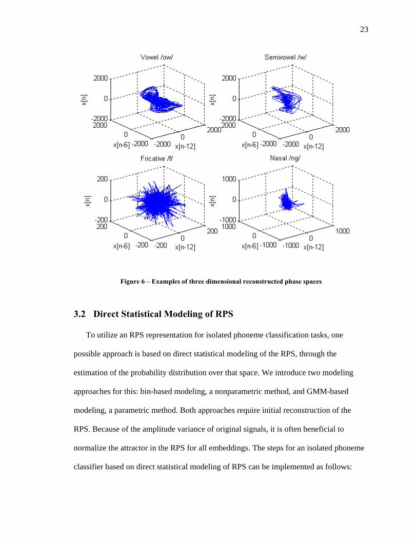
Examples of reconstructed phase spaces of phonemes are shown in Figure 6, by
plotting the row vectors of the trajectory matrix. The trajectory pattern within the phase
space is referred to as its attractor, defined as a bounded subset of the phase space to
which trajectories asymptote as time increases [36]. As can be seen from the plots,
different types of phonemes demonstrate different geometric structures in the RPS. The
vowel /ow/ exhibits clear structure probably due to the periodic nature of its waveform
originated from voiced source excitation. The semivowel /w/ and nasal /ng/ exhibit less
clear structure than the vowel. The fricative /f/ exhibits the random noise like structure
indicating its origin from unvoiced noise excitation.
23
Figure 6 – Examples of three dimensional reconstructed phase spaces
3.2 Direct Statistical Modeling of RPS
To utilize an RPS representation for isolated phoneme classification tasks, one
possible approach is based on direct statistical modeling of the RPS, through the
estimation of the probability distribution over that space. We introduce two modeling
approaches for this: bin-based modeling, a nonparametric method, and GMM-based
modeling, a parametric method. Both approaches require initial reconstruction of the
RPS. Because of the amplitude variance of original signals, it is often beneficial to
normalize the attractor in the RPS for all embeddings. The steps for an isolated phoneme
classifier based on direct statistical modeling of RPS can be implemented as follows:

24
1. Determine the time lag and embedding dimension of the RPS and normalize the
attractors through a radial normalization method:
,nn
rσ−
= Xx µx (3.4)
where is an original point in the phase space, nx Xµ is the mean of the columns of
, and X
( ) ( )
2
21 1
1 .1
N
rn dN d τ
στ = + −
−− − ∑ Xx µn (3.5)
2. Model the probability distribution of the attractor of the RPS through either a
nonparametric approach or a parametric approach.
3. Use a maximum likelihood classifier (discussed in Section 3.3) to perform
classification based on the probability distribution obtained from step 2.
3.2.1 Bin-based Distribution Modeling
A discrete statistical characterization (estimates of the probability masses) of the
reconstructed phase space is formed by dividing the reconstructed phase space into n by n
histogram bins as is illustrated in Figure 7 [37]. This is done by dividing each dimension
into n partitions such that each partition contains approximately 1/n of all training data
points. To compute bin boundaries, all training data are embedded into phase spaces, and
vectors of RPSs are combined together.

25
Figure 7 – Dividing RPS into bins for PMF estimation
The estimate of the probability mass function within each bin can be calculated via
ˆ ( ) .Number of points in bin xp xTotal number of points
= (3.6)
For our experiments, each dimension is assigned ten partitions. In the case of two-
dimensional RPS, this gives a 10 by 10 grid to form a 100-bin probability mass function.
3.2.2 GMM-based Distribution Modeling
The bin-based method is difficult to apply to higher dimensional RPSs because of
scalability issues. Firstly, all training data need to be embedded into phase spaces and
combined together to determine the intercepts. For a large dataset and higher dimensional
RPS, this will create huge space complexity. Secondly, bin-based modeling is a
nonparametric approach. As the dimension of the RPS increases, the number of bins

26
increases exponentially. To address this, a second approach is introduced, based on
statistical modeling using GMMs, as introduced in Section 2.2, to form a parametric
distribution to estimate the PDF of RPS. It is a parametric approach, and the number of
parameters of the GMM only increases linearly (with a diagonal covariance matrix and
same number of mixtures) as the dimension of the RPS increases. The EM training will
finish in polynomial time, thus the GMM does not have the same scalability problems as
a bin-based system does.
3.3 Classifier
Classification is done through a Maximum Likelihood (ML) [38] classifier that uses
the estimates of the distribution from the direct statistical modeling of each RPS. This
classifier computes the conditional probabilities of the different classes given the phase
space and then selects the class with the highest likelihood:
( ){ } (1 1 1
ˆarg max | arg max |N
i i i n ii C i C n
c p c p= = =
)ˆ c⎧ ⎫= = ⎨ ⎬
⎩ ⎭∏X
… …x (3.7)
where is the likelihood of a point in the phase space, C is the number of phoneme
classes, and c is the resulting maximum likelihood class.
ˆ ( )i np x
3.4 Datasets and Software
TIMIT [39, 40] database is used for these experiments. TIMIT contains a total of
6300 sentences, 10 sentences spoken by each of 630 speakers from 8 major dialect
regions. There are total of 1260 SA sentences, 3150 SX sentences and 1890 SI sentences.
Each speaker says 2 SA sentences, 5 SX sentences and 3 SI sentences. The SA sentences
27
are dialect sentences that expose the dialectal variants of the speakers and are read by all
speakers. The SX sentences are phonetically-compact sentences designed to provide a
good coverage of phonemes. The SI sentences are phonetically-diverse sentences that add
diversity in sentence types and phonetic contexts. When doing training and testing, only
SX sentences and SI sentences are used, while the SA sentences are discarded to avoid
overlap of training and testing material.
TIMIT is an ideal database for isolated phoneme classification experiments because it
contains expertly labeled, phonetic level transcription and segmentation performed by
linguists. It can be used for continuous recognition as well. The sampling rate of TIMIT
is 16kHz and the data are digitized using 16 bits. The training partition and testing
partition are predefined. There is no overlap of speakers of training set and testing set,
which means the experiments are speaker-independent.
There are a total of 64 possible phonetic labels in TIMIT. From this set, 48 phonemes
are modeled. When generating confusion matrix, certain within-group errors are not
counted. This folds 48 phonemes to 39-phoneme class for calculating the results [41].
Matlab [42] is a technical computing language and is largely involved in this
research. The Hidden Markov Toolkit (HTK) [26] is a set of speech recognition toolkit
widely used in the speech community for HMM modeling. Other software tools used
include Netlab [28], TSTOOL [43], and TISEAN [44]. The Netlab toolbox is designed to
provide a wide range of data analysis and modeling functions. TSTOOL and TISEAN are
nonlinear time series analysis tools. Apart from Matlab, all the above tools are free and
available online.
28
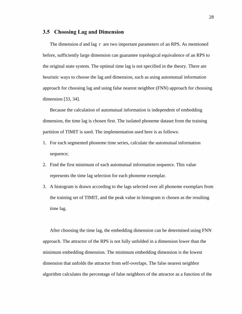
3.5 Choosing Lag and Dimension
The dimension d and lag τ are two important parameters of an RPS. As mentioned
before, sufficiently large dimension can guarantee topological equivalence of an RPS to
the original state system. The optimal time lag is not specified in the theory. There are
heuristic ways to choose the lag and dimension, such as using automutual information
approach for choosing lag and using false nearest neighbor (FNN) approach for choosing
dimension [33, 34].
Because the calculation of automutual information is independent of embedding
dimension, the time lag is chosen first. The isolated phoneme dataset from the training
partition of TIMIT is used. The implementation used here is as follows:
1. For each segmented phoneme time series, calculate the automutual information
sequence;
2. Find the first minimum of each automutual information sequence. This value
represents the time lag selection for each phoneme exemplar.
3. A histogram is drawn according to the lags selected over all phoneme exemplars from
the training set of TIMIT, and the peak value in histogram is chosen as the resulting
time lag.
After choosing the time lag, the embedding dimension can be determined using FNN
approach. The attractor of the RPS is not fully unfolded in a dimension lower than the
minimum embedding dimension. The minimum embedding dimension is the lowest
dimension that unfolds the attractor from self-overlaps. The false nearest neighbor
algorithm calculates the percentage of false neighbors of the attractor as a function of the

29
embedding dimension. As this percentage drops to a small enough value, the attractor is
considered to be unfolded, and the embedding dimension is identified. The
implementation used here is adopted from [34]. The idea is to compare the distance
between the nearest neighbor points in dimension d+1 to that in dimension d. If the
distance in the higher dimension is substantially larger than in the lower dimension, then
those points are false neighbors, which means the dimension is not high enough to unfold
the current point in the attractor. The algorithm is implemented as follows:
1. Let be the phase space point defined in Equation (3.2), where d is current the
embedding dimension. Find the nearest neighbor of ;
( )n dx
( )n dx
2. Compute the square of the Euclidian distance between the nearest neighbor points for
both dimension d and dimension d+1; denoted as and respectively; 2 ( )nD d 2 ( 1nD d + )
3. Compute the ratio 2 2( 1) ( )
( )n n
n
D d D dD d+ −
, and compare this ratio to a threshold ; If
the ratio exceeds the threshold, the current point is a false neighbor;
1r
( )n dx
4. Calculate the percentage of all points that are false neighbors and compare this
percentage to another threshold ; If the percentage is small enough, then the
attractor is fully unfolded and the dimension can be determined.
2r
5. A histogram is drawn according to the dimensions selected over the training set from
TIMIT and the peak value in histogram is chosen as the embedding dimension.
It is important to notice that the two thresholds affect the selection of dimension. For
clean data, the percentage of false nearest neighbors can be expected to drop to near zero
as embedding dimension increases. The second threshold is set to a very small number

30
such as 0.001 with TIMIT database. The first threshold is usually empirical and the
value of 15 is adopted from [34].
1r
The following results shown here use the segmented isolated phonemes with the
length of at least 200 points. This guarantees that each time series has adequate points for
calculating automutual information sequence as well as FNNs in higher dimension.
Different phonetic classes can have different lag and dimension selections, so five
phonetic classes are investigated, given by:
Vowels ih ix ax ah ao aa iy eh ey ae aw ay ox ow uh uw er
Affricates and Fricatives sh zh jh ch s z f th v dh
Semivowels and glides el l r w y hh
Nasals n en m ng
Stops b d g p t k dx
The isolated phoneme exemplars are extracted from the training set of TIMIT for the
experiments. There are more than 100,000 total phonetic exemplars in this set. The
number of exemplars is large enough to generalize the results.
The figures shown below are the histograms of first minimum of automutual
information across different phonetic classes, as well as overall. From the histogram of
all phonemes, we can see that the lag peaks at five or six, with six representing the peak
value. In subclass histogram plots, vowels and semivowels/glides have peak at lag of 6,
while the peaks occur at lag of 1, 9 and 3 for affricates/fricatives, nasals and stops
respectively.

31
Figure 8 – Histogram of first minimum of automutual function for all phoneme
Figure 9 – Histogram of first minimum of automutual function for vowels

32
Figure 10 – Histogram of first minimum of automutual function for affricates and fricatives
Figure 11 – Histogram of first minimum of automutual function for semivowels and glides

33
Figure 12 – Histogram of first minimum of automutual function for nasals
Figure 13 – Histogram of first minimum of automutual function for stops
34
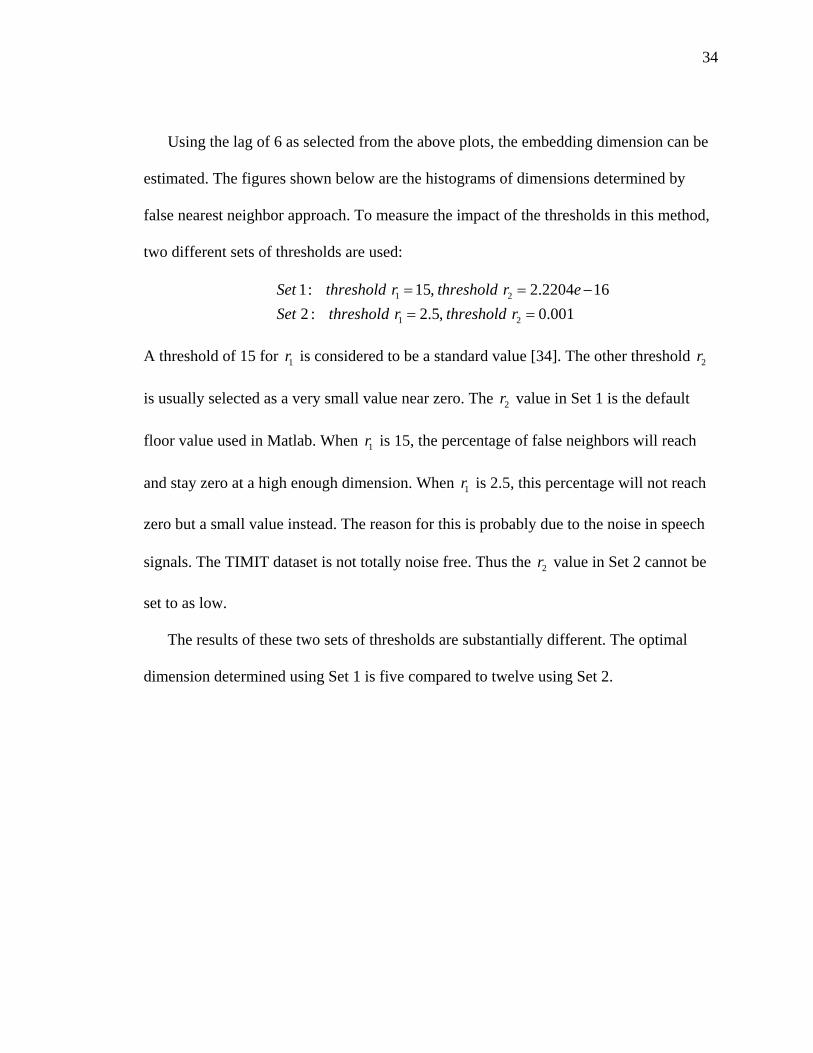
Using the lag of 6 as selected from the above plots, the embedding dimension can be
estimated. The figures shown below are the histograms of dimensions determined by
false nearest neighbor approach. To measure the impact of the thresholds in this method,
two different sets of thresholds are used:
1 2
1 2
1: 15, 2.2204 162 : 2.5, 0.001
Set threshold r threshold r eSet threshold r threshold r
= = −= =
A threshold of 15 for is considered to be a standard value [34]. The other threshold
is usually selected as a very small value near zero. The value in Set 1 is the default
floor value used in Matlab. When is 15, the percentage of false neighbors will reach
and stay zero at a high enough dimension. When is 2.5, this percentage will not reach
zero but a small value instead. The reason for this is probably due to the noise in speech
signals. The TIMIT dataset is not totally noise free. Thus the value in Set 2 cannot be
set to as low.
1r 2r
2r
1r
1r
2r
The results of these two sets of thresholds are substantially different. The optimal
dimension determined using Set 1 is five compared to twelve using Set 2.

35
Figure 14 – Histogram of dimension by FNN approach (Set 1) for all phonemes
Figure 15 – Histogram of dimension by FNN approach (Set 1) for vowels

36
Figure 16 – Histogram of dimension by FNN approach (Set 1) for affricates and fricatives
Figure 17 – Histogram of dimension by FNN approach (Set 1) for semivowels and glides

37
Figure 18 – Histogram of dimension by FNN approach (Set 1) for nasals
Figure 19 – Histogram of dimension by FNN approach (Set 1) for stops

38
Figure 20 – Histogram of dimension by FNN approach (Set 2) for all phonemes
Figure 21 – Histogram of dimension by FNN approach (Set 2) for vowels

39
Figure 22 – Histogram of dimension by FNN approach (Set 2) for affricates and fricatives
Figure 23 – Histogram of dimension by FNN approach (Set 2) for semivowels and glides
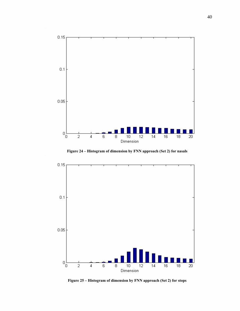
40
Figure 24 – Histogram of dimension by FNN approach (Set 2) for nasals
Figure 25 – Histogram of dimension by FNN approach (Set 2) for stops

41
The above results suggest that the optimal lag and dimension using this heuristic
approach would be a lag of 6 and a dimension of 5 (using standard thresholds). The
actual best value of lag and dimension based on performance of an RPS based speech
recognition system could be different than the results from this heuristic approach. Thus
it is worth running some experiments to compare this lag and dimension according to
actual performance. The task used for this purpose is isolated phoneme classification. A
GMM is used for modeling the distribution of RPS and a maximum likelihood classifier
is utilized. The details will be discusses in next section. The results are presented here in
order to compare the different approaches on selecting lag and dimension. Because a lag
of six is determined by the heuristic approach, Figure 26 shows the classification
accuracy across a wide range of dimensions on TIMIT using lag of 6.
Figure 26 – TIMIT Accuracy vs. dimension at lag of 6

42
The peak value of the above figure is at dimension of 11 and it reaches a plateau after
that point. In light of this observation, another set of TIMIT isolated phoneme
classification experiments are performed using dimension of 11 but varying the lag. The
results are shown in Figure 27. The peak is at lag of 1 with a second peak at lag of 5. The
best values for lag and dimension are one and eleven respectively as concluded from the
actual the phoneme classification tasks. The selection of dimension is not restricted as
long as a high enough dimension is chosen according to the figure above.
Figure 27 – TIMIT Accuracy vs. lag at dimension of 11
Since the task of applying RPS based method is to perform speech recognition, it
makes sense to choose the lag and dimension according to actual system performance on
43
development data. In the experiments in Chapter 5 involving speech recognition tasks
over complete TIMIT database, a lag of 1 and dimension of at least 10 are used.
3.6 Issues of Speech Signal Variability using RPS Based Method
Variability exists in speech signals. Different speakers and different environments can
affect the robustness of a speech recognition system. In speaker-independent tasks, the
attractor structures are affected by the variance of speakers. Inconsistency of attractor
structures across different speakers would be expected to result in poor performance. The
noise in speech signals could also have negative impact on attractor patterns that lead to
poor statistical modeling. Other factors, such as fundamental frequency and RPS
transformation, could also affect the attractor structure. The RPS representation of speech
signals is different from the cepstral representation, and it is of interest to analyze the
impact of such variabilities for this time-domain representation. The experiments
presented in the following sections address three factors that could have impact on speech
recognition accuracy using the RPS based method [45, 46].
3.6.1 Effect of Principal Component Analysis on RPS
Principal component analysis is also known as Karhunen-Loeve transform. It is used
for reducing dimensionality while retaining the subspace that has largest variance. Using
PCA, the original feature space is transformed to another feature space on a different set
of orthogonal base. The basis vectors of the principal component analysis are the
eigenvectors of the covariance matrix of a given distribution. In practice, the basis
vectors can be computed from the eigenvectors of the autocorrelation matrix. The
44
smallest eigenvalues can be discarded for dimension reduction purpose as they
correspond to least effective features. The transformed feature vector has a diagonal
covariance matrix and therefore is particularly useful for models based on Gaussian
distribution features.
In order to truly represent the underlying dynamic systems that produce the speech
signals, usually a high dimensional phase space reconstruction is required. Considering
the computational cost associated with the phase space method, a lower dimensional
phase space reconstruction is usually desired in practice. By doing PCA transformation
over the phase space, the eigenspaces that retain the most significant amount of
information are kept. Previous work on transformation over phase space can also be
found in the literature [47].
PCA over the RPS is performed in following steps:
1. A trajectory matrix is compiled as shown in Equation (3.3).
2. A scatter matrix is formed
(3.8) TS = X X
and an eigendecomposition is performed such that
(3.9) TS = ΦΛΦ
where the eigenvalues of are reordered in non-increasing order along the diagonal. Λ
3. Select the largest eigenvalues, and let ′Φ be a matrix containing the corresponding
columns of . Then Φ
′=Y XΦ (3.10)
is the new PCA projected trajectory matrix.

45
Three types of projection are implemented. The difference between each
implementation mainly depends on the various ways to compute and apply
transformations over the data set.
• PCA projection
The PCA projection method learns one scatter matrix from all the training data
and applies the PCA transformation to the trajectory matrix from each phoneme.
• Individual projection
The individual projection method learns and applies the transformation to the
trajectory matrix from each phoneme on an example-by-example basis.
• Class-based projection
The class-based projection method involves two steps in implementation. In the
training phase, it learns a scatter matrix for each phoneme class (e.g. vowels,
nasals, stops, fricatives, and semivowels) and applies the transformation over each
phoneme based on its known class identification. In the test phase, several
different transformations, one for each class, are done on the trajectory matrix of
each test phoneme exemplar, and these projected trajectory matrices are used to
compute probabilities under the corresponding class models for the Maximum
Likelihood classifier.
The TIMIT corpus is used to train and evaluate the isolated phoneme classification
task. The embedding dimensions before and after PCA projection are 15 and 3
respectively for all the experiments.
The speaker-dependent experiment uses data from one male speaker with 417
phoneme exemplars over standard 48 phonemes [41]. Classification results with three

46
types of projection are obtained from the speaker-dependent experiments, giving a
comparison between the different implementations mentioned above.
The speaker-independent test uses training data from six male speakers and testing
data from three different male speakers with experiments run on three types of phonemes
respectively. A total of 7 fricatives, 7 vowels, and 5 nasals are selected for these
experiments. Also, classification results with three types of projection are obtained from
the speaker-independent experiments, giving an idea of how the projection over the phase
space affects the classification accuracy on different types of phonemes.
Table 1 shows the results of speaker-dependent experiments on a total of 48 phonemes
with and without projection. Table 2 shows the results of speaker-independent
experiments on a total of 7 fricative phonemes with and without projection. Table 3
shows the results of speaker-independent experiments on a total of 7 vowel phonemes
with and without projection. Table 4 shows the results of speaker-independent
experiments on a total of 5 nasal phonemes with and without projection.
Without Proj.
PCA Proj.
Individual Proj.
Class-based Proj.
24.33% 28.47% 25.30% 11.19%
Table 1 – Results of speaker-dependent 48 phonemes using PCA on RPS
Without Proj.
PCA Proj.
Individual Proj.
Class-based Proj.
39.07% 42.38% 33.77% 29.14%
Table 2 – Results on speaker-independent fricatives using PCA on RPS

47
Without Proj.
PCA Proj.
Individual Proj.
Class-based Proj.
40.54% 43.24% 29.68% 8.78%
Table 3 – Results on speaker-independent vowels using PCA on RPS
Without Proj.
PCA Proj.
Individual Proj.
Class-based Proj.
55.21% 48.96% 47.92% 48.96%
Table 4 – Results on speaker-independent nasals using PCA on RPS
The basic PCA projection method works best for the overall, fricative, and vowel
phoneme classification tasks, while the class-based projection method gives the lowest
classification accuracies for these tasks. It can be observed that some phonemes tend to
be classified as one particular phoneme for both fricative and vowel experiments using
class-based projection method. The confusion of these phonemes in the reconstructed
phase space using distribution model can be observed by investigating the confusion
matrices for each case.
3.6.2 Effect of Vowel Pitch Variability
Fundamental frequency, as a parameter that varies significantly but does not contain
information about the generating phoneme, should affect the phase space in an adverse
way for classification. The basic idea introduced here for dealing with vowel pitch
variability is to use variable time lags instead of a fixed time lag for embedding vowel
phonemes, as a function of the underlying fundamental frequency of the vowel. An
48
estimate of the fundamental frequency is used to determine the appropriate embedding
lag.
The fundamental frequency estimate algorithm for vowels used here is based on the
computation of autocorrelation in the time domain as implemented by the Entropic ESPS
package [48].
The typical vowel fundamental frequency range for male speakers is 100~150Hz,
with an average of about 125Hz, while the typical range for female speakers is
175~256Hz, with an average of about 200Hz. For this experiment only male speakers are
used. In the reconstructed phase space, a lower fundamental frequency has a longer
period, corresponding to a larger time lag. With a baseline time lag and mean
fundamental frequency given as τ and 0f respectively, we perform fundamental
frequency compensation via the equations
0 0f fτ τ ′ ′= (3.11)
and
0
0
' ff
ττ =′
(3.12)
where τ ′ is the new time lag and 0f ′ is the fundamental frequency estimate of the
phoneme example. This time lag is rounded and used for phase space reconstruction, for
both estimation of the phoneme distributions across the training set and maximum
likelihood classification of the test set examples.
Two different baseline time lags are used in the experiments. A time lag of six
corresponds to that chosen through examination of the automutual information heuristics;
however, rounding effects lead to quite a low resolution on the lags in the experiment,

49
which vary primarily between 5, 6, and 7. To achieve a slightly higher resolution, a
second set of experiments at a time lag of 12 is implemented for comparison. Since the
final time lags used for reconstruction are given by a fundamental frequency ratio, the
value of the baseline frequency is not of great importance, but should be chosen to be
near the mean fundamental frequency. A baseline of 129Hz was used, as the mean
fundamental frequency of the training set. The final time lag is given in accordance with
Equation (3.12) above.
A seven-vowel set is used for these experiments. Data are selected from 6 male
speakers for training and 3 different male speakers for testing, all within the same dialect
region.
There are four experiments, two with a baseline lag of 6 and two with a baseline lag
of 12. In each case, the tests are run with a fixed lag as well as with variable lags. The
four experiments are summarized as follows:
Exp 1: 2, 6,d τ τ τ′= = = ,
Exp 2: 00
0
2, 6, 129 , fd f Hzf
ττ τ ′= = = =′
,
Exp 3: 2, 12,d τ τ τ′= = = ,
Exp 4: 00
0
2, 12, 129 , fd f Hzf
ττ τ ′= = = =′
where d is the embedding dimension, τ is the default time lag, 0f is the baseline
fundamental frequency, 0f ′ is the estimated fundamental frequency, and τ ′ is the actual
embedding time lag.
Table 5 shows the resulting ranges for τ ′ given the parameters, while Table 6 and
Table 7 show the classification results.

50
τ 0f τ ′ 6 129Hz 5~8
12 129Hz 10~15
Table 5 – Range of τ ′ given τ and 0f
Exp 1 Exp 2 27.70% 36.49%
Table 6 – Vowel phoneme variable lag classification results for lag of 6
Exp 3 Exp 4 39.19% 38.51%
Table 7 – Vowel phoneme variable lag classification results for lag of 12
As can be seen from the above results, the improvement of classification accuracy is
obtained by using a variable lag model with baseline lag of 6. The classification accuracy
is almost unchanged with baseline lag of 12. The results suggest that the variability of
fundamental frequency is not large.
3.6.3 Effect of Speaker Variability
Speaker variability is an unknown factor with regard to the amount of variance
caused in underlying attractor characteristics, and is an important issue in the question of
how well the RPS technique will work for speaker-independent tasks. Initial experiments
have shown some significant discriminability in such tasks, but performed at a
measurably lower accuracy than that for speaker-dependent tests [46].
Using the phase space reconstruction technique for speaker-independent tasks clearly
requires that the attractor pattern across different speakers is consistent. Inconsistency of

51
attractor structures across different speakers would be expected to lead to smoothed and
imprecise phoneme models with resulting poor classification accuracy. The experiments
presented here are designed to investigate the inter-speaker variation of attractor patterns.
Although a number of different attractor distance metrics could be used for this purpose,
the best such choice is not readily apparent and we have instead focused on classification
accuracy as a function of the number of speakers in a closed-set speaker dependent
recognition task. The higher the consistency of attractors across speakers, the less
accuracy degradation should be expected as the number of speakers in the set is
increased.
All speakers are male speakers selected from the same dialect region within the
TIMIT corpus. The only variable is the number of speakers for isolated phoneme
classification tasks.
To examine speaker variability effects across different classes of phonemes, vowels,
fricatives and nasals are tested separately. The overall data set is a group of 22 male
speakers, from which subsets of 22, 17, 11, 6, 3, 2 and 1 speaker(s) have been randomly
selected. Classification experiments are performed on sets of 7 fricatives, 7 vowels, and 5
nasals.
The evaluation of speaker variability was carried out using leave-one-out cross
validation. The overall classification accuracies for the three types of phonemes are
shown in Table 8, Table 9 and Table 10.
Spkr# 1 2 6 11 17 22
Acc(%) 58.00 51.06 49.26 49.02 47.98 48.58
Table 8 – Classification results of fricatives on various numbers of speakers

52
Spkr# 1 2 6 11 17 22
Acc(%) 61.90 49.09 49.58 46.92 45.46 46.03
Table 9 – Classification results of vowels on various numbers of speakers
Spkr# 1 2 3 6 11 17 22
Acc(%) 51.79 40.00 31.91 29.95 29.71 27.79 26.76
Table 10 – Classification results of nasals on various numbers of speakers
Figure 28 is a visual representation of the results presented above. The classification
results are plotted against the number of speakers for vowels, fricatives and nasals
respectively.
Figure 28 – The classification accuracy vs. number of speakers

53
As can be seen from Figure 28, the degree of attractor variation across speakers is
different for these three types of phonemes. Nasals appear to have the largest variability
while the fricatives have the least. In all three phoneme types, the accuracy is relatively
unchanged after 2 or 3 speakers. The results show that the accuracy reaches asymptote as
larger number of speakers is included in the experiments. The speaker variability does
exist but basic attractor structures are consistent, which can be captured by statistical
modeling of RPSs.
3.7 Summary
This chapter has introduced theory for the reconstructed phase space approach to
signal representation, and addressed issue of choosing parameters for phase space
embedding. Two types of direct statistical modeling on RPS have been presented. A
maximum likelihood classifier is used for RPS based classification. The issues of speech
signal variability using RPS based method were also thoroughly investigated. The next
chapter will introduce frame-based analysis to RPSs, which can reduce time complexity
and make continuous speech recognition possible using RPSs with the current HMM
framework.

54
4. Frame-based Features from Reconstructed Phase Spaces 4.1 Why use Frame-based Features
In a conventional HMM, the probability of state occupancy decreases exponentially
with time:
(4.1) ( ) (1 ).ti ii id t a a= − i
The probability of t consecutive observations in state i is the probability of taking the
self-loop at state i for t times. The traditional speech recognition system uses frame-based
features, with frame sizes anywhere between 10ms to 40ms. The RPS based method
described above regards each point in the phase space as a feature vector, thus the feature
vector from RPS representation can change as fast as the sampling rate. For a typical
16kHz-sampling rate (e.g. TIMIT database), the feature rate would be 160 times faster
than a 10ms frame step size used with cepstral features. In this case, the default HMM
state duration shown in Equation (4.1) cannot be used for continuous speech recognition.
There are some ways to cope with this problem. One way is to use HMM with an
explicit time duration distribution for each state. Another way is to mimic the traditional
MFCC features based on frame-by-frame speech signal analysis. The second approach
has two major advantages over the first one: the simplicity and the reduced computational
time. There is no easy way to incorporate an explicit duration model into HMMs for use
with point-by-point RPS feature vectors. By using the frame-based feature extraction
approach, the existing continuous speech recognition framework can be utilized without
any change on HMM state duration. Also, the direct statistical modeling approach on
RPSs for isolated phoneme classification tasks can be replaced by this frame-based
approach for reduced computational time.
55
4.2 Frame-based Features from RPS
Several nonlinear features can be useful in speech applications, such as the
information in the LPC residue, the correlation dimension of speech signal, physiological
parameters related to the speech production system [15, 49], and high order statistics of
the acoustic measurements. Some frame-based features, such as modulations, fractals,
correlation dimensions, Lyapunov exponents, etc., have been used in speech recognition
[16-18, 50, 51]. But still few speech recognition systems exploit these acoustic features.
The perspective of this work is on investigating new frame-based features from
reconstructed phase space for speech recognition. The proposed SVD derived features
from trajectory matrix of RPS can be extracted on frame-by-frame basis and will be
introduced in the following section.
4.3 SVD Derived Features
There are two different implementations of SVD projection on RPSs to extract
features. The first one uses global SVD projection and the second one uses regional SVD
projection. Both methods can extract features from RPSs on one frame length of data.
4.3.1 Global SVD Derived Features
The steps for extracting the global SVD derived features are as follows:
1. Frame the speech signal with given frame length and step size. In the experiments, a
25ms window and 10ms step size are used. TIMIT has a 16kHz-sampling rate, so
25ms corresponds to 400 points and 10ms corresponds to 160 points.

56
2. Embed each frame of signal into RPS, and create a trajectory matrix from each frame
( )
( )
( ) ( )( )
1 11 1
2 22 1
( 2) 1 1
d
d
N N d N d N d d
x x x
x x x
x x x
ττ
ττ
τ τ τ
++ −
++ −
− − − − − − ×
⎡ ⎤⎢ ⎥⎢⎢⎢ ⎥⎢ ⎥⎣ ⎦
⎥⎥
2 T
as shown in Equation (3.3).
3. Compile frame-based trajectory matrices from all training data into a larger trajectory
matrix . X
4. Factorize the trajectory matrix using singular value decomposition: X
(4.2) = TX USV
where S is a diagonal matrix containing the singular values of X with decreasing
order, and and are matrices of the singular vectors associated with . In
practice, the matrix is obtained by doing SVD on instead of , such that
U V S
V TX X X
(4.3) T T T TX X = (USV ) (USV ) = VS V
The advantage of doing SVD on is that is of size d by d, where d is the
embedding dimension, thus it can be obtained from all training data by accumulating
this covariance value calculated from each frame without memory or space
complexity problems.
TX X TX X
5. After getting matrix V , calculate the new SVD projected trajectory matrix for both
training and testing data on frame-by-frame basis:
(4.4) X = XV
By projecting into the basis vectors in , the new trajectory matrix has been
orthogonized because its covariance matrix is close to a diagonal matrix.
V
6. Calculate the diagonal values of the covariance matrix of the new trajectory matrix:

57
(4.5) ˆ ˆ(diag TX X)
2
These diagonal values obtained from Equation (4.5) are the elements of the feature
vector.
The obtained features can be thought of as the power values along the main principle
axes in the RPS. There are some useful properties of this decomposition. The singular
vectors in are actually the eigenvectors of , and the singular vectors in are the
eigenvectors of the covariance matrix . The singular values in S are square roots of
the eigenvalues of both and . The new trajectory matrix has orthogonal
property as can be proven by calculating the covariance:
U TXX V
TX X
TXX TX X
(4.6) ˆ ˆT T T T T T TX X = (XV) (XV) = V X XV = V (VSU )(USV )V = S
In practice, matrix V is calculated separately from all training data, the obtained
covariance matrix of is not an exact diagonal matrix. But the diagonal values selected
as the feature elements should have dominant information over non-diagonal elements.
X
4.3.2 Regional SVD Derived Features
In addition to the probability density information of the RPS, trajectory information
can be used to characterize changes in the attractor. It is beneficial to incorporate such
information since the trajectory information could have discriminatory power in cases
where two RPSs may have similar density distribution. The regional SVD approach
divides the RPS into eight regions and extract feature element from each region. These
feature elements are combined to form the final feature vector. The trajectory change in

58
attractor can be somewhat reflected in the change of value of feature element from each
region.
The steps for extracting the regional SVD derived features are as follows:
1. Follow the same steps 1 to 4 from global SVD approach to obtain matrix V.
2. Let be a matrix containing first 3 by 3 block of V (corresponding to the three
largest singular values of S). Project higher dimensional trajectory matrix into three
dimensional matrix using matrix
′V
′V :
′ ′X = XV (4.7)
is now the trajectory matrix of three dimensional phase space. ′X
3. Partition to eight regions using three planes: ′X 0, 0, 0x y z= = = . The
corresponding points in original higher dimensional trajectory matrix X are likewise
partitioned into eight groups.
4. Within each region, use the same procedure to extract feature elements as with global
SVD. There are eight different projection matrices V’s to train in this case, one for
each region.
5. If three feature elements are extracted from each region, then the final feature vector
will have 24 elements in total.
4.4 Implementation for Speech Recognition Tasks
The implementation for speech recognition tasks using SVD derived features is
similar to an MFCC based speech recognition system because both systems employ
frame-based feature extraction scheme. A 12 dimensional RPS embedding can usually
59
have 12 SVD derived feature elements in accordance to typical 12 MFCC feature vector.
Deltas and Delta-Deltas can also be computed on SVD features using linear regression
introduced in Equation (2.10). An energy measure can also be appended to the feature
vector. For experiments with SVD derived features, the energy is computed as the log of
the signal energy based on one frame of speech { , 1, , }ns n N= … [26]:
2
1log
N
nn
E=
= s∑ (4.8)
The same HMM structure and training and testing algorithms can be utilized for both
isolated speech recognition and continuous speech recognition.
4.5 Summary
This chapter discussed the necessity of extracting frame-based features. The singular
value decomposition was proposed in use with trajectory matrix of RPS to extract such
features. Two SVD projections, the global SVD projection and the regional SVD
projection, were introduced. The implementation of such feature extraction methods was
elaborated. The frond-end frame-based feature extraction from RPS can work with
current speech recognition systems directly.
60
5. Experimental Setup and Results
5.1 RPS Isolated Phoneme Classification
The time lag and dimension used here for the experiments are based on the criteria
elucidated in Section 3.5. Because classification accuracy is the decisive factor of the
experiments, the selection of time lag and dimension is based on this criterion from
previous experiments. For RPS isolated phoneme classification experiments using SVD
derived feature sets, a lag of 1 and dimension of 12 are chosen. In most cases, the feature
vector extracted from 12 dimensional RPS consists of 12 elements using SVD method.
The number of elements is the same as the traditional MFCC feature vector has.
Additional features such as log energy and Delta and Delta-Delta are also calculated the
same way as MFCCs. In general, the number of GMM mixtures affects the classification
accuracy in that the higher the number of mixtures, the lower the classification error. Too
large a number of mixtures can have huge computational cost and overfitting problem on
training data. The experiments presented here show the results of using different number
of mixtures for the purpose of comparison. The window size is 25 ms (400 sample points)
and frame step size is 10 ms (160 sample points) for all experiments.
5.1.1 Baselines
The baseline results are shown here in order to compare the current state-of-the-art
system with our frame-based RPS method. The baseline system uses MFCC features as
described in Chapter 2. Most of the parameters use the default value from HTK. The
configuration file can be found in the appendix. A simple 1-state HMM topology with a
GMM state distribution is utilized. Table 11 shows the baseline results on different

61
number of mixtures, and different set of features (12-MFCC denotes standard 12 MFCC
coefficients feature vector; 13-MFCC+E denotes feature vector comprised of standard 12
MFCC coefficients and log energy; 39-MFCC+E+∆,∆∆ denotes feature vector comprised
of standard 12 MFCC coefficients and log energy and their 1st order and 2nd order linear
regression coefficients.)
# of mixtures 16 128 512
12-MFCC 50.34 52.08 52.12
13-MFCC+E 51.09 53.40 55.81
39-MFCC+E+∆,∆∆ 54.86 59.19 59.78
Table 11 – Baseline phoneme accuracy
5.1.2 Experiments using Frame-Based SVD Derived Features
The basic feature vector is computed from each frame using the same window size
and step size as the MFCC feature. The original speech signal of each frame is embedded
directly into an RPS without imposing any windowing function. All RPSs are normalized
via Equations (3.4) and (3.5). Features are extracted through the procedure described in
Chapter 4. A lag of 1 and a dimension of 12 are used for phase space embedding, so that
the basic SVD feature vector is comprised of 12 elements. Log energy is computed via
Equation (4.8). The 1st order and 2nd order linear regression coefficients are computed the
same way as MFCC.
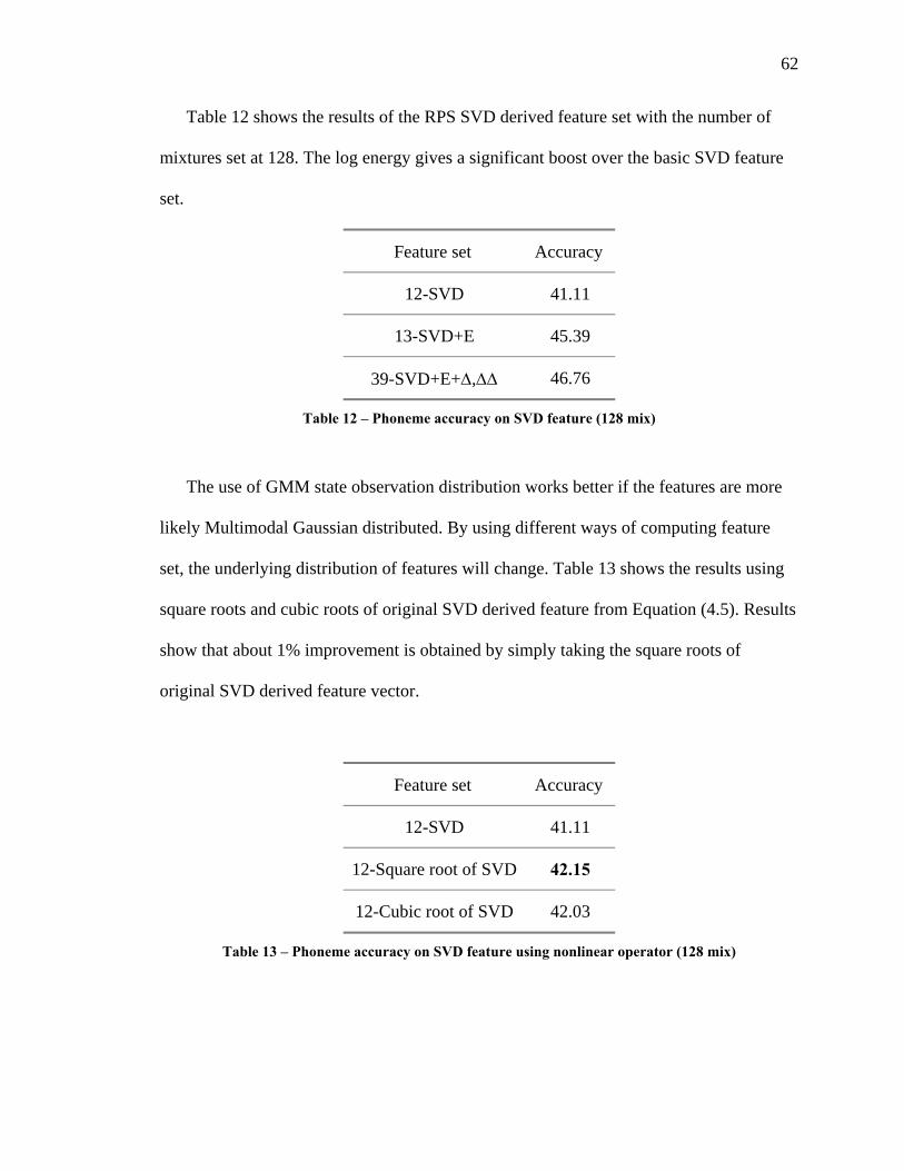
62
Table 12 shows the results of the RPS SVD derived feature set with the number of
mixtures set at 128. The log energy gives a significant boost over the basic SVD feature
set.
Feature set Accuracy
12-SVD 41.11
13-SVD+E 45.39
39-SVD+E+∆,∆∆ 46.76
Table 12 – Phoneme accuracy on SVD feature (128 mix)
The use of GMM state observation distribution works better if the features are more
likely Multimodal Gaussian distributed. By using different ways of computing feature
set, the underlying distribution of features will change. Table 13 shows the results using
square roots and cubic roots of original SVD derived feature from Equation (4.5). Results
show that about 1% improvement is obtained by simply taking the square roots of
original SVD derived feature vector.
Feature set Accuracy
12-SVD 41.11
12-Square root of SVD 42.15
12-Cubic root of SVD 42.03
Table 13 – Phoneme accuracy on SVD feature using nonlinear operator (128 mix)

63
The regional SVD derived feature is expected to give better results since it is
supposed to capture geometric information in attractor pattern. Table 14 presents the
results of a regional SVD experiment. The regional SVD experiment utilizes a 24-
element feature vector, with 3 elements extracted from each of the eight projected
regions. The basic 12-element SVD feature result and 30-element SVD feature result
(derived from an RPS of dimension of 30) are also included for comparison. With even
fewer feature elements, the regional SVD feature set still outperforms the 30-element
SVD feature set. This demonstrates the trajectory information is captured by the regional
SVD approach.
Feature set Accuracy
12-SVD 41.11
30-SVD 42.17
24-Regional SVD 43.54
Table 14 – Phoneme accuracy on regional SVD feature (128 mix)
The results with SVD derived features also show good robustness to noise. In
preliminary experiment of isolated phoneme classification under noisy environment, the
clean TIMIT corpus is contaminated with Gaussian white noise such that the signal to
noise ratio is 5dB. The classification accuracy drops from 41.1% to 37.1%, which is 4.0%
net degradation. In the experiment using MFCC feature with the same level noise
contamination, the classification accuracy drops from 54.9% to 36.3%, which is 18.6%
net degradation. In this case, the SVD derived RPS feature outperforms the traditional
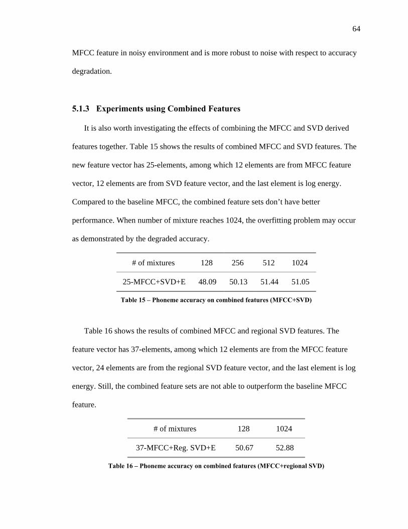
64
MFCC feature in noisy environment and is more robust to noise with respect to accuracy
degradation.
5.1.3 Experiments using Combined Features
It is also worth investigating the effects of combining the MFCC and SVD derived
features together. Table 15 shows the results of combined MFCC and SVD features. The
new feature vector has 25-elements, among which 12 elements are from MFCC feature
vector, 12 elements are from SVD feature vector, and the last element is log energy.
Compared to the baseline MFCC, the combined feature sets don’t have better
performance. When number of mixture reaches 1024, the overfitting problem may occur
as demonstrated by the degraded accuracy.
# of mixtures 128 256 512 1024
25-MFCC+SVD+E 48.09 50.13 51.44 51.05
Table 15 – Phoneme accuracy on combined features (MFCC+SVD)
Table 16 shows the results of combined MFCC and regional SVD features. The
feature vector has 37-elements, among which 12 elements are from the MFCC feature
vector, 24 elements are from the regional SVD feature vector, and the last element is log
energy. Still, the combined feature sets are not able to outperform the baseline MFCC
feature.
# of mixtures 128 1024
37-MFCC+Reg. SVD+E 50.67 52.88
Table 16 – Phoneme accuracy on combined features (MFCC+regional SVD)

65
5.2 RPS Continuous Speech Recognition
Because the SVD derived RPS feature set is based on frame-by-frame analysis, it can
be applied to continuous speech recognition (CSR) directly. Preliminary CSR results are
shown in Table 17. A 3-state HMM topology with an 8-mixture GMM are used. The
language model is a bigram trained on training set of TIMIT. A total of 46 monophones
is modeled as the basic speech unit.
The percentage Word Correct is defined as:
100%,N D SCorrectN
− −= × (5.1)
and the percentage Word Accuracy is defined as:
100%,N D S IAccuracyN
− − −= × (5.2)
where S, D, I, and N are the number of substitution errors, the number of deletion errors,
the number of insertion errors, and the total number of labels in the reference
transcriptions, respectively.
Word Correct Word Accuracy
13-MFCC+E 26.10 23.38
39-MFCC+E+∆,∆∆ 46.20 41.83
13-SVD+E 17.35 13.57
39-SVD+E+∆,∆∆ 18.38 10.59
Table 17 – CSR results (3-state monophone HMM, 8 mix, bigram)
66
Although traditional MFCC features still outperform SVD RPS features in CSR
experiments, the features from RPS have shown significant discriminatory power and
they may have the potential to contribute to improved performance of speech recognition
systems.
5.3 Discussion
This chapter presented results using alternative features from time domain analysis of
speech, namely SVD derived RPS features, on isolated phoneme classification and
continuous speech recognition tasks. There are several issues that could have impact on
the results. It is important to consider these issues in order to achieve improved
performance of speech recognition.
The origin of SVD derived features is from the time domain and is different from
MFCC features originated from frequency domain. It is unclear why the combination of
MFCC and SVD feature is not helpful on boosting the accuracy. By investigating the
confusion matrices of MFCC and SVD feature sets, we can observe that the
corresponding phonemes have some major classification overlaps between these two.
One conjecture is that the SVD features may contain similar information as the MFCC
features. In order to combine them together to get better performance, a more
sophisticated combination mechanism may be helpful. The distribution of SVD features
is different from the MFCC features. From the results presented here, we can conclude
that the SVD features usually need larger numbers of mixtures to achieve asymptotic
accuracy compared to MFCC features. The GMMs are supposed to capture arbitrary

67
distribution but may not be the most effective way of representing RPS SVD derived
feature space.
The experiments on noisy environment show the robustness of the SVD time domain
approach. The application of using time domain features in robust speech recognition is
promising and worth further investigation.
68
6. Conclusions and Future Work
6.1 Conclusions
Speech recognition using a dynamical systems approach has been presented in the
thesis. This is a novel approach that extracts features from the time-domain using
reconstructed phase spaces. The results indicate that RPS features have substantial
discriminatory power in speech recognition application. The study of nonlinear
dynamical system shows that the RPS is able to capture the nonlinear information of
underlying system that cannot be captured by frequency domain analysis alone.
The two parameters of an RPS, time lag and embedding dimension, play an important
role both theoretically and practically of building a speech recognition system based on
time domain features. In theory, a sufficient dimension is required to embed the signals in
order to fully unfold the attractors in the RPSs. Both the heuristic approach and the
empirical approach introduced here for determining the embedding dimension suggest
that there exists a lowest embedding dimension that would truly unfold the attractor. A
dimension of 10-12 would be a good choice for speech recognition application using the
RPS based method, as indicated by the results shown here. Unlike the embedding
dimension, the time lag does not affect system performance in a monotonic way. An
empirical study suggests that a higher dimension combined with a smaller time lag would
be a good choice for better system performance. One such choice is a dimension of 12
and a lag of 1, as used in the SVD experiments.
The features from RPSs can be used in speaker-independent tasks as demonstrated by
the speaker-independent experiments presented in this thesis. In general, the SVD feature
extraction approach has better accuracy than the direct statistical modeling approach on

69
RPSs, but still behind the traditional MFCC features by a net gap of about 10% in
accuracy. But the results are promising. The combination of traditional frequency domain
features and time domain features has the potential of building better speech recognition
systems if it is done in an intelligent way.
In conclusion, this research applies nonlinear techniques to speech, and brings a
totally different perspective for the speech recognition problem that has been traditionally
dominated by a linear system analysis approach.
6.2 Future Work
The research on this topic is at its beginning and further work is needed in order to
further understand this topic. The RPS based approach has the potential for identifying
noise robust features. The robustness issue is critical in real world speech applications
and worth investigation in future work. With frame-based features from RPS, it is
possible to improve continuous speech recognition. Issues such as the HMM topology,
frame size, step size, temporal change of features, modeling technique, RPS
normalization, and feature normalization and transformation, could all affect the overall
system performance, and have not all been studied thoroughly.
Traditional MFCC features stem from approximation of the human auditory
perception system. The features from the RPS, however, have no clear physical meaning.
This technique can be applied to virtually any type of time series. It is of necessary to
strengthen the theoretical framework for applying such techniques to speech recognition.
In light of this, it seems necessary to investigate the relationship between RPSs and
speech production systems in order to build a nonlinear speech production model that

70
could identify effective acoustic features. There are also possible ways of characterizing
RPSs using alternative representations, such as geometric measures, invariants from
RPSs, moments, global flow reconstructions, fixed points identification of the attractor,
or higher order features from SVD. A modification of the SVD method, such as using
higher order SVD moments, may be possible to obtain better features that capture higher
order information from the underlying signal.
71
7. References
[1] J. W. Forgie and C. D. Forgie, "Results Obtained from a vowel recognition computer program," Journal of the Acoustic Society of America, vol. 31, pp. 1480-1489, 1959.
[2] D. R. Reddy, "An approach to computer speech recognition by direct analysis of the speech wave," Computer Science Dept., Stanford University Techical Report No. C549, Sept. 1966.
[3] L. Rabiner and B. H. Juang, Fundamentals of speech recognition. Englewood Cliffs, NJ, 1993.
[4] L. R. Rabiner, S. E. Levinson, A. E. Rosenberg, and J. G. Wilpon, "Speaker Independent Recognition of Isolated Words Using Clustering Techniques," IEEE Transactions on Acoustics, Speech and Signal Processing, vol. 27, pp. 336-349, 1979.
[5] L. R. Rabiner, "Tutorial on Hidden Markov Models and Selected Applications in Speech Recognition," Proceedings of the IEEE, vol. 77, pp. 257-286, 1989.
[6] J. R. Deller, J. H. L. Hansen, and J. G. Proakis, Discrete-Time Processing of Speech Signals, Second ed. New York: IEEE Press, 2000.
[7] X. Huang, A. Acero, and H.-W. Hon, Spoken Language Processing. Upper Saddle River, New Jersey: Prentice Hall, 2001.
[8] B. Gold and N. Morgan, Speech and Audio Signal Processing. New York, New York: John Wiley and Sons, 2000.
[9] H. Hermansky, "Perceptual linear predictive (PLP) analysis for speech recognition," Journal of the Acoustical Society of America, pp. 1738-1752, 1990.
[10] H. Hermansky, N. Morgan, and H. G. Hirsch, "Recognition of speech in additive and convolutional noise based on RASTA spectral processing," proceedings of IEEE International Conference on Acoustics, Speech, and Signal Processing, 1993, pp. 83-86.

72
[11] S. Haykin, Adaptive Filter Theory, 4th ed. Upper Saddle River, NJ: Prentice Hall, 2001.
[12] G. Kubin, "Nonlinear Speech Processing," in Speech Coding and Synthesis, W. B. Kleijn and K. K. Paliwal, Eds.: Elsevier Science, 1995.
[13] A. Kumar and S. K. Mullick, "Nonlinear Dynamical Analysis of Speech," Journal of the Acoustical Society of America, vol. 100, pp. 615-629, 1996.
[14] J. D. Farmer and J. J. Sidorowich, "Exploiting chaos to predict the future and reduce noise," in Evolution, Learning, and Cognition, Y. C. Lee, Ed. Singapore: World Scientific, 1988, pp. 277-330.
[15] H. M. Teager and S. M. Teager, "Evidence for nonlinear sound production mechanisms in the vocal tract," proceedings of NATO ASI on Speech Production and Speech Modelling, 1990, pp. 241-261.
[16] P. Maragos, J. F. Kaiser, and T. F. Quatieri, "Energy separation in signal modulations with application to speech analysis," IEEE Transactions on Signal Processing, vol. 41, pp. 3024-3051, 1993.
[17] P. Maragos and A. Potamianos, "Fractal Dimensions of Speech Sounds: Computation and Application to Automatic Speech Recogntion," Journal of Acoustical Society of America, vol. 105, pp. 1925-1932, 1999.
[18] D. Dimitriadis, P. Maragos, and A. Potamianos, "Modulation features for speech recognition," proceedings of IEEE International Conference on Acoustics, Speech, and Signal Processing, 2002, pp. I-377-I-380.
[19] N. H. Packard, J. P. Crutchfield, J. D. Farmer, and R. S. Shaw, "Geometry from a time series," Physical Review Letters, vol. 45, pp. 712-716, 1980.
[20] F. Takens, "Detecting strange attractors in turbulence," proceedings of Dynamical Systems and Turbulence, Warwick, 1980, pp. 366-381.
[21] T. Sauer, J. A. Yorke, and M. Casdagli, "Embedology," Journal of Statistical Physics, vol. 65, pp. 579-616, 1991.
73
[22] M. Banbrook and S. McLaughlin, "Is Speech Chaotic?," proceedings of IEE Colloquium on Exploiting Chaos in Signal Processing, 1994, pp. 8/1-8/8.
[23] M. Banbrook, S. McLaughlin, and I. Mann, "Speech characterization and synthesis by nonlinear methods," IEEE Transactions on Speech and Audio Processing, vol. 7, pp. 1 -17, 1999.
[24] R. O. Duda, P. E. Hart, and D. G. Stork, Pattern Classification, 2nd ed. New York, New York: John Wiley & Sons, 2001.
[25] S. Stevens and J. Volkman, "The relation of pitch to frequency: A revised scale," American Journal of Psycholinguistics, vol. 53, pp. 329-353, 1940.
[26] S. Young, G. Evermann, D. Kershaw, G. Moore, J. Odell, D. Ollason, D. Povey, V. Valtchev, and P. Woodland, The HTK Book: Cambridge University, 2002.
[27] K. Fukunaga, Introduction to statistical pattern recognition, 2nd ed: Academic Press, 1990.
[28] I. Nabney, Netlab: Algorithms for Pattern Recognition. London: Springer-Verlag, 2002.
[29] A. P. Dempster, N. M. Laird, and D. B. Rubin, "Maximum likelihood from incomplete data via the EM algorithm," Journal of the Royal Statistical Society, Series B, vol. 39, pp. 1-38, 1977.
[30] T. K. Moon, "The Expectation-Maximization Algorithm," in IEEE Signal Processing Magazine, 1996, pp. 47-59.
[31] F. Jelinek, Statistical Methods for Speech Recognition. Cambridge, MA: MIT Press, 1999.
[32] L. E. Baum, "An inequality and associated maximization technique in statistical estimation for probabilistic functions of Markov processes," Inequalities, vol. 3, pp. 1-8, 1972.
[33] H. Kantz and T. Schreiber, Nonlinear Time Series Analysis. Cambridge: Cambridge University Press, 2000.

74
[34] H. D. I. Abarbanel, Analysis of observed chaotic data. New York: Springer, 1996.
[35] H. Whitney, "Differentiable Manifolds," The Annals of Mathematics, 2nd Series, vol. 37, pp. 645-680, 1936.
[36] E. Ott, Chaos in dynamical systems. Cambridge, England: Cambridge University Press, 1993.
[37] J. Ye, R. J. Povinelli, and M. T. Johnson, "Phoneme Classification Using Naive Bayes Classifier In Reconstructed Phase Space," proceedings of IEEE Signal Processing Society 10th Digital Signal Processing Workshop, 2002, pp. 2.2.
[38] T. M. Mitchell, Machine Learning. New York: McGraw-Hill, 1997.
[39] J. Garofolo, L. Lamel, W. Fisher, J. Fiscus, D. Pallett, N. Dahlgren, and V. Zue, "TIMIT Acoustic-Phonetic Continuous Speech Corpus," Linguistic Data Consortium, 1993.
[40] V. Zue, S. Seneff, and J. Glass, "Speech Database Development at MIT: TIMIT and Beyond," Speech Communication, vol. 9, pp. 351-356, 1990.
[41] K.-F. Lee and H.-W. Hon, "Speaker-independent phone recognition using hidden Markov models," IEEE Transactions on Acoustics, Speech and Signal Processing, vol. 37, pp. 1641-1648, 1989.
[42] The MathWorks Inc., "Matlab," Version 6.5, 2002.
[43] C. Merkwirth, U. Parlitz, I. Wedekind, and W. Lauterborn, "TS Tools," available at http://www.physik3.gwdg.de/tstool/index.html, 2001, cited 2002.
[44] R. Hegger, H. Kantz, and T. Schreiber, "Practical implementation of nonlinear time series methods: The TISEAN package," Chaos, vol. 9, 1999.
[45] J. Ye, M. T. Johnson, and R. J. Povinelli, "Phoneme Classification over Reconstructed Phase Space using Principal Component Analysis," proceedings of ISCA Tutorial and Research Workshop on Non-linear Speech Processing (NOLISP), Le Croisic, France, 2003, pp. 11-16.

75
[46] J. Ye, M. T. Johnson, and R. J. Povinelli, "Study of Attractor Variation in the Reconstructed Phase Space of Speech Signals," proceedings of ISCA Tutorial and Research Workshop on Non-linear Speech Processing (NOLISP), Le Croisic, France, 2003, pp. 5-10.
[47] D. S. Broomhead and G. King, "Extracting Qualitative Dynamics from Experimental Data," Physica D, pp. 217-236, 1986.
[48] Entropic, ESPS Programs Manual: Entropic Research Laboratory, 1993.
[49] H. M. Teager, "Some observations on oral air flow during phonation," IEEE Transactions on Acoustics, Speech and Signal Processing, vol. 28, pp. 599-601, 1980.
[50] P. Maragos, A. G. Dimakis, and I. Kokkinos, "Some advances in nonlinear speech modeling using modulations, fractals, and chaos," proceedings of 14th International Conference on Digital Signal Processing, 2002, pp. 325-332.
[51] V. Pitsikalis and P. Maragos, "Speech analysis and feature extraction using chaotic models," proceedings of IEEE International Conference on Acoustics, Speech, and Signal Processing, Orlando, Florida, 2002, pp. I/533-I/536.


