Hitotsubashi Journa] of Economics 27 Special Issue (1986) 57-74. C The Hitotsubashi Academy
STAGFLATION IN THE INDUSTRIAL COUNTRIES =
AN UPDATED OVERVIEW
MICHAEL BRUNO
I. Introduction
Some twelve to fifteen years ago, in the early 1970s, a series of dramatic worldwide
developments brought to an end a prolonged period of rapid growth and low unemployment in the industrial countries. There ensued a new phase that can be termed the stagflation
era, marked by waves of high inflation, slow economic growth and rising unemployment.
Two major worldwide events can be singled out to have marked the start of the new
era. The Bretton Woods international monetary system collapsed in 1971 and ever since
we have had a quasi-flexible rate regime with highly volatile exchange rates between the
major currencies. Next, in 1973 the oil price shock and the commodity price boom was the first and largest of exogenous price shocks that afilicted the world system in the 1970s.
At present, five years after the second oil price shock, with a considerable glut in world oil
and extreme weakening of the OPEC cartel one may safely assume that large oil shocks are unlikely to recur in the foreseeable future although fluctuations in commodity prices of
smaller amplitude may continue to characterize the world macroeconomy. Exchange rate volatility, however, is still very much with us, greatly exacerbated by the enormous
flows of financial assets which were largely enhanced by the recycling of petro-dollars after
OPEC I. Exchange rate movements in response to real interest rate differentials caused
by a particular policy mix in the U.S. have had a marked effect over the more recent devel-
opments of inflation and unemployment among the major partners of the industrial world.
Also some of the structural problems that first emerged in the late 1960s, in particular the
rigidity of labour markets in Europe, are still there and they too account for some of the
more recent differences in development among the major industrial countries.
This paper will provide an updated overview of the major fluctuations that have taken
place over the last fifteen years with particular emphasis on the role of supply factors, such
as import and labour cost developments and on the interplay of supply with the continued
major role of aggregate demand fluctuations. Sectlon 11 gives a general empirical introduc-
tion followed by a brief theoretical discussion of the role of supply and demand factors in
the macroeconomy (Section 111). Section IV applies some of the underlying theoretical
considerations to the analysis of unemployment, particularly to account for the persistently
rising unemployment in Europe. Section V analyses the main factors underlying differential
inflationary performance among countries, putting special emphasis on import prices and
exchange rate movements. This is followed by discussion of the role of U.S. policy and

58 HITOTSUBASHI JOURNAL OF EcoNoMlcs the international policy coordination problem in recent years.
[October
II. Empirica/ Background
Table I provides a summary of the main data on GNP and productivity growth, the change in unemployment and the rate of inflation for the period 1960-85. The latter is
broken down into six sub-periods: pre-OPEC I normal growth (1960-73), the first oil shock
(OPEC I, 1973-75), the post-shock recovery (1975-79), the second oil shock (OPEC II,
1979-81), the recent recovery (1981-84) and the most recent OECD Economic Outlook forecast for 1985-86. To minimize country detail we have here only given summary data
for the U.S., Japan, the EEC country bloc and the OECD total.l
The table shows the sharp slowdown in GNP and productivity growth after 1973. There
was virtually a standstill during the two OPEC shock periods but even during the two re-
TABLE 1. GROWTH OF PRODUCT, PRODUCTIVITY, UN,EMPLOYMENT, AND INFLATro~~!', 196(~1986
Historical growth OPEC-I
73-75 60-73
GNP growth
U.S. 4. Japan I O. EEC 4. OECD 5.
Productivity growth
U,S. 2. Japan 8 . EEC 4 . OECD 3 . Rise in unemployment
U.S. 1 Japan O. EEC O. OECD O . Inflationb
U.S. 3. Jap an 5 . EEC 4 . OECD 4 .
2 4
o
4 5 9
4(t
2a 3(:~
6a
4 5 o 4
-o. 8 o. 6
-o. 3 o. 3
-1. 1
1. O
O. 7
O. 1
3. 5
O. 6
l.5
2. O
10. O
18. 2
13. O
l 2. 4
Recovery OPEC-II 75-79 79-81
4. 7
5. 3
3. 6
4. o
O. 8
3* 9
3. 1
2. 4
-2. 5 O. 2
l. 1
-O. 1
6. 7
10. 4
9. 1
8. 4
O. 9
3. 4
-O. 3 1. 2
O. 2
2. 8
O. 9
1. O
1.7 O. 1
2. 2
1.6
11.7 5. 5
10. 8
11, 1
Recovery
8 1 -84
2. 8
4. 2
1. 3
2. 4
l. 2
3. O
1.9
1.9
-O. 1 O. 5
3. O
1.5
4. 5
2. 3
7. 8
6. 1
Pro jected
85-86
3. o
4, 9
2. 3
3, o
l. O
3. 5
2. O
l.9
- O. 3
- O. 2
O. 5
O. 1
3, 4
2. 3
5, o
4, 8
a. 1969-73. b, Rise in consumer price index; the period breakdown here differs slightly: 1974-75, 1975-78, 1978-81.
Sources: 196(~81~IMF (IFS) and OECD Economic Outlook data. 1985-86-0ECD Economic Outlook, June 1985.
l The country detail is given in the sources cited in the table. The analysis in Bruno and Sachs (1985) also includes a substantial country breakdown for Europe. The OECD total includcs, in addition to the countries represented in the table, also the European countries not in EEC (in particular the Scandinavian countries) as well as Canada and Australiasia.

1986] STAGFLATION IN THE INDUSTRIAL COUNTRIES : AN UPDATED OVERVIEW 59
coveries growth has never returned to its pre-OPEC Ievels. At present both output and
productivity growth are back to approximately one half of their annual rates in the 1960s,
the only exception being the U.S. for which output and employment growth (this can be
obtained by approximately adding up the respective numbers in the first two blocks of Table
1) is presently between 2/3 and 3/4 of its historical rates.
Slow growth has its counterpart in unemployment which, however, differed across the
major country groupings. The U.S. is virtually the only country in which unemployment
fluctuated back and forth as between the different phases shown in Table l, unemployment
being back to where it had been ten years ago. Japan, which has shown low unemployment
throughout the period, with only minor changes, can probably not be compared on the
same basis. Europe as a whole and virtually all European countries individually have shown a systematic increase in unemployment throughout the stagflation era with the most
marked increase taking place during and particularly since OPEC II, up to the present.
Next we note the pattern of inflation (see the last block of Table 1)-a sharp acceleration
for all countries during OPEC I followed by a deceleration during the first recovery. The
OPEC 11 period witnessed another inflationary wave, with the exclusion of Japan. In the
more recent recovery the deceleration in inflation rates was more marked and by now (1985-
86) inflation is more or less back, on average, to where it had been in the glorious sixties
(again Japan is an exception with inflation down to 2.3~~ from 5.5~~ in the sixties). Gener-
ally the pattern of inflation has been much more varied as between different countries, rang-
ing across countries and during price shock periods anywhere between 5~ and 20~ (with
few higher exceptions like Turkey and lceland). We shall subsequently link these differences
mainly to the cost side, the behaviour of wages and in particular import prices. The latter,
in turn, are highly dependent on differential exchange rate movements.
These data raise a number of interesting questions on some of which considerable re-
search has been conducted in recent years. First and foremost is to account for what looks
like a marked worldwide departure from the inflation and unemplotment cycles of earlier
decades, namely episodes in which inflation accelerates and unemployment rises simultane-
ously, or a shift from southwest to northeast in the unemployment-inflation framework, see
the periods 73-74 and 79-80 in Figure I for the U.S. and EEC respectively, preceded by very
steep "conventional" portions of the curve). On the other hand the two recovery periods
(75-79 and 81 to the present) Iook much more like conventional northwest to southeast
shifts down the Phillips curve. Macroeconomic Theory has to account for both types of
phenomena within the same framework (to be identified as aggregate supply and aggregate
demand shifts). Next on the agenda is the marked difference in response of the major countries partic-
ularly after the second oil shock. We note, in particular, the difference in response to the
second oil shock in Japan, as compared to OPEC I. We also note for special consideration
the marked difference between the U.S. and Europe in respect to both inflation slowdown
and unemployment changes in the last recovery (cf, the two curves of Figure I for the years
1980-84). In the next section we shall give a very general discussion of the aggregate supply
and aggregate demand factors that have played the main role in the overall inflation and
unemployment patterns, and then take up separately the issue of country differences in
unemployment and in inflation in subsequent sections.

60
FIGURE I .
U.S.A
~6 14
~: o c~
- 12 Y~ ~:
10
8
6
4
2
o
HITOTSUBASHI JOURNAL OF ECONOMICS
E.E.C. INFLATION AND UNEMPLOYMENT, 1959-1984, INFLATION AND UNEMPLOYMEN_ T, 1 968-1984
74 80
74 . / 76 f-{ +~
l 1 l l l l l l a
~ . / 78-
71 72 __~l~~~-~ .~ ~~ ¥ ~7 71 h68 ¥ f
~l l 'l
5 9 72
80 f ¥ / ¥ ¥
,, ¥ +++, ¥
~¥¥ tX/ 75
¥ // ¥¥
¥ / ¥ ¥ / ¥ ¥ / ¥1/ 76
84~~
82
¥ ¥
¥82
E.E.C.
84
[October
64
63
60
U.S.A.
~8~3
2
4
6 8 10 %
Unem ployment
III. Aggregate Supply and Aggregate Demalid in the Short Run
A macroeconomic framework within which the effects of input-price shocks can be analyzed requires the explicit incorporation of raw materials (n) as a separate factor of pro-
duction along with the conventional labour (1) and capital (k) inputs in the production of
final goods (q). The determination of output and prices in a system like this can be de-
scribed in terms of aggregate supply (S) and aggregate demand (D) schedules, as drawn in
Figure 2.2 Along the horizontal axis we measure gross output quantity of final goods and
along the vertical axis the price of these goods (p) re]ative to the domestic price of a com-
petitive basket of goods, p* +e, where p* represents the world price of final goods and e
the exchange rate. The relative price measured along the vertical axis in Figure 2 will be
denoted by lr(=p-p* -e). This relative price is also the reciprocal of what is sometimes
termed the "real exchange rate."3
Two other relative prices play a major role in accounting for aggregate shifts in this
system. One is the relative world price or real cost of material inputs (1r~=p*~-p*), where
p** is the nominal world price of materials. The other is the real cost of labour, w,(=w-p., where w is the nominal wage and w, is measured in the units of some final basket of goods, p., here-consumption goods).
' For a detailed analysis see Bruno and Sachs (1985), chap. 5. 3 We here define variables in terms of their logarithrns and therefore the product of the exchange rate and
the world price, which is the domestic price of the world good, will be the sum of the logarithms (p*+e) and the ratio of the two prices is the difference of the logarithms [p-(p*-e)1.

1986] STAGFLATION IN THE INDUSTRIAL COUNTRIES : AN UPDATED OVERVIEW
FIGURE 2. AGGREGATE SUPPLY AND AGGREGATE DEMAND SHIFTS
61
_:~ '* l ~~)
~:~ '.
~ ¥ ¥ // ~~~~1e S ¥ C/ ~~~: ~
ll B' B~~/ I A 'TO ~ -------~:----r-----l I rl ~~~~ / <~,~~ :
'rl ~ IT~(1~ f ~~~ l ------ J
I ~:,/ ' J'# ll / : I¥ } I / ¥ I I I) I l / I I I I / I I I E¥ l l I l ~ l I
¥l i I : ~¥t~_ ' I I t D l i l I ~ l l l l
q~ qb qc qa q
The aggregate supply of goods in the short run can be described as an upward-sloping
curve, S, where the productive capacity (represented here by capital stock, k), the level of
technology or total factor productivity (T), and the real cost of the two variable factors of
production, materials and labor (i.e., 1?~ and lv*, respectively), are held constant. The curve
S is the marginal short-run cost schedule which assumes rising marginal costs of production
with an increase in output. Below a certain output level, as capacity becomes underutilized.
the supply curve may be horizontal, while above a certain output level S may become fairly
steep as full employment of all factors in the economy is reachrd. Under fairly reasonable
assumptions it can be argued that an increase in the real cost of either materials (1r^) or labour
(w.) will shift the supply curve (S) up and to the left while an increase in the capital stock
(k) or in total factor productivity (T) will in the long run shift S down and to the right.4
The curve D marks the aggregate demand schedule for this economy. Other things being equal, the demand for final goods (such as consumer goods or exports) rises with a
fall in the relative final goods price (1r). What are the parameters shifting the aggregate de-
mand curve? One is the relative price of materials (It~) which affects demand through real
income and wealth, and not only on the supply side. When the real price ofmaterials such
as oil rises, a net importer of such goods suffers a real income loss while a net exporter (such
as OPEC) benefits. For a typical OECD country a rise in the real cost of material inputs
shifts the aggregate demand schedule to the left (this・is why IT* is placed on the left hand side of D in Figure 2). A rise in the real world income (y*), which affects export demand, or
expansionary demostic fiscal and monetary policy (briefly denoted by FM in Figure 2), which
affects domestic demand for consumption and investment goods, will each shlft the D curve
' The various parameters are thus marked on the respective sides of the curve S in Figure 2.

62 HITOTSUBASHI JOURNAL OF ECoNoMlcs [october up and to the right.
We can now use this framework to analyze the output and price effects of rising ma-
terial prices as well as the derived effects coming from the policy response to such input-
price shocks. The first impact of rising input prices is a leftward shift of the aggregate
supply curve (from S to S')-rising costs of material inputs reduce profits and the output
that producers will be willing to supply at each given relative price level. Suppose for a
moment that there is sufficient compensatory expansionary policy on the demand side to
neutralize the contractionary effect of rising material prices on real income, so that the de-
mand curve (D) stays put. In this hypothetical case, with everything else (including real
wages) held constant, rising material prices cause a move of the economy from the equi-
librium point A to a new equilibrium point C. There is a fall in output and a rise in prices,
which are the essence of a stagflationary impact effect. Such supply shock is in marked con-
trast to a shift in aggregate demand, with S held constant, where prices and output tend
to move together (compare, for example, the points A and E). Note that a similar effect
would be observed if there is an autonomous real wage push, exceeding productivity growth.
The size of the supply shock depends on what happens to real wages. If real wages are downward flexible, thus mitigating the squeeze on profits, this in itself may impart a
compensatory rightward shift in the S curve. If wages are rigid, or rising, relative to pro-
ductivity (T), the leftward shift in S, for a given upward push on material prices, will be
more pronounced. The associated profit squeeze which hampers investment depresses capital growth (the change in k), which may further strengthen the supply shock in the med-
ium and long run. Consider the demand side now. Other things being equal, a rise in -,.^, we have argued,
depresses real income and demand for a net importer, thus shifting the D schedule leftward
and imparting further downward pressure on output (and employment). Contractionaly demand-management policy (a fall in FM) and the mutual interaction of falling incomes in export markets of other industrial countries (reducing y*) cause a further contraction
of aggregate demand. Suppose D shifts to D'. A new equilibrium in the commodity market, given the con-
figuration of Figure 2, will be at the point B, output having fallen further to qb and the final-
goods relative price also falling in this case (a real depreciation) from lro to ITr5 The price
level need not fall, however, since this also depends on what happens to world prices of
final goods (p*) and to the exchange rate (e). If ~ is downward rigid then production may
actually take place at B' (a further fall in demand and output to qb), where a disequilibrium
between supply and demand (potential excess supply of B'B") may for a time persist.
The "pure" case of a supply shock, bringing about both unemployment and inflation
is generally understood to have characterized the period both immediately and after the
first oil and commodity price shock, the extent of resulting stagfiation in various countries
depending on the extent of real wage rigidity. Such shift from southwest to northeast in
the unemployment-inflation framework has also characterized the second oil shock. An added leftward bias of the aggregate supply curve in the 1970s may have been caused by
the depressive effect of the profit squeeze on capital accumulation. All of these have im-
parted a "classical" element to the unemployment which has certainly not been present in
earlier, cyclical unemployment episodes. However, even the developments immediately
" When both S and D contract the outcome for " may obviously go either way

1986] STAGFI_ATION IN THE INDUSTRIAL COUNTRlES : AN UPDATED OVERVIEW 63
following the two oil shocks cannot be understood without explicit regard being paid to
contractionary forces coming from leftward shifts in the aggregate demand schedules of countries.
Table 2 gives the acceleration in unemployment and inflation as well as changes in
two supply factors (relative import prices and real wages) and one demand factor6 (real
money supply) during the two OPEC periods. Employment as well as output can be shown to have been negatively related to real import prices and real wages and positively related
to money and government deficits. Both types of factors were thus operative in the ob-
served direction during the oil shock periods, except for differences in respect to real wage
TABLE 2. CHANGE IN GROWTH RATES, SELECTED VARIABLES, DURlNG OPEC I AND OPEC II
Unemploy-men t (1)
Acceleration in 1973-75a
U.S. 3. 5 Japan O. 6 France I . 5 Germany 2. 8 Italy - O. 4 U.K. 1. 5 Belgium 2. 3 Denmark -Netherlands I . 7 Average 7 EC I . 6
Total OECD 2, O Acceleration in 1979-8lb
U.S. I . 8 Japan O. 1 France I . 7 Germany I , l Italy O. 8 U.K. 5. 6 Belgium 2, 5 Denmark -Netherlands 3. 3 Average 7 EC 2. 5 Total OECD I . 7
Infiation (2)
5. 2
11.5
6. 9
2. 2
13. 1
13. 1
8. 3
5. 8
3. 6
7. 6
7. O
4. 2
O. 3
3. 8
l.9
4, 9
1. 5
O. 8
2. 1
O. 7
2. 2
3. O
Relative import pnces (3)
8. 7
17. 9
8. 1
6. 4
12. 9
12. O
1. l
7. 1
3. 2
7. 4
6. 6
6. 4
20. 7
3. 5
5. 3
4, O
-1.7 1. O
6. 8
2. 6
2. 5
4. 7
Real
wage (4)
-2. 9
-4. 2
1.7
-2. 4 - O. 6
-1.5 1.5
1.4
1.2
O. 2
-5 8 -2 5
-2. 8
-1.9 -2. 4
l. 5
O. 6
O. 1
-3, O
-1. 1
Real
money supply
(5)
-7. O
-20. 4
-1.8 1.2
-20. 8
-6. 4 4. 3
15 1. 6
-4 1
-6. 5
-5. 6
-2. 8
-9. O
- 15. 7
-5. 6
-5. 6
-O. 8
-6. O
-4. 6
Notes: Unemployment-change during period. Other variables-rate of growth in 1973-75 compared with 1967-73; 1979-81 compared with 1975-79. Real wage-nominal wage (IMF, IFS data) defiated by consumer prices. Col. (4) of the second panel is the difference between 1978-81 and 1975-78 except for
the U.S, and Denmark (1978-80). Real money supply-MI deflated by consumer prices.
a. Change in growth rates compared to 1967-73.
b. Change in grovrth rates compared to 1975-79.
Sources : OECD Historical Statistics and Economic Outlook, except for wages.
6 Figures for the government deficit can be read out of Table 3.
HITOTSUBASHI JOURNAL OF EcoNoMlcs
behaviour among countries. Real wage flexibility appears to have had a mitigating effect
in the case of the U.S. and Japan, but not in most European countries shown, at least until
OPEC 11 (a more precise statement will be made in the next section). Another aspect of
the same phenomenon is the sharp profit squeeze (for which no separate data are shown
here). This partly explains the large drop in investment after OPEC I and a more moderate
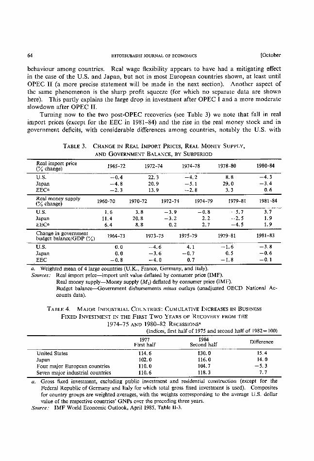
slowdown after OPEC II. Turning now to the two post-OPEC recoveries (see Table 3) we note that fall in real
irnport prices (except for the EEC in 1981-84) and the rise in the real money stock and in
government deficits, with considerable differences among countries, notably the U.S. with
TABLE 3. CHANGE IN REAL IMPORT PRICEs, REAL MoNEY SUPPLY, AND GOVERNMENT BALANCE, BY SUBPERIOD
Real import price (~( change)
U.S.
Japan
EECa Real money supply (~ change)
U.S. Ja pan
EECa
1965-72
- o. 4
-4. 8
-2. 3
1 972-74
1960-70 197 0-72
l. 6
11.4 6. 4
Change in government 1964-73 budget balance/GDP (~)
U.S.
Japan
EEC
o. o
o. o
- o. 8
3. 8
20. 8
8. 8
22. 3
20. 9
13. 9
1972-74
1973-75
-4. 6 - 3. 6
-4. o
-3.9 -3. 2
o. 2
1974-78
-4. 2
-5. 1
-2. 8
1974-79
1975-79
4. 1
- O. 7
O. 7
- o. 8
2. 2
2. 7
1978-80
8. 8
29. o
3. 3
1980-84
-4. 3 - 3. 4
o. 6
1979-81 1981-84
-5.7 -2. 5
-4. 5
1979-81
-1.6 O. 5
-1.8
3. 7
1.9
1.9
1981-83
-3. 8 - O. 6
-O. l
a. Weighted mean of 4 Iarge countries (U.K., France, Germany, and Italy).
Sources: Real import price-import unit value deflated by consumer price (IMF).
Real money supply-Money supply (Ml) deflated by consumer price aMF).
Budget balance-Government disbursements minus outlays (unadjusted OECD National Ac-counts data).
TABLE 4. MAJOR INDUSTRIAL COUNTRIES : CUMULATIVE INCREASES IN BUS1NESS FIXED INVESTMENT IN THE FIRST TWO YEARS OF RECOVERY FROM THE
1974-75 AND 1980-82 RECESSIONS~ (Indices, first half of 1975 and second half of 1982= 100)
United States
Japan Four major European countries
Seven major industrial countries
1 977
First half
1 14. 6
102. O
l 10. O
110. 6
l 984
Second half
130. O
116. O
104.7
118. 3
Difference
15. 4
14. O
-5. 3
7,7
a. Gross fixed investment, excluding public investment and residential construction (except for the
Federal Republic of Germany and Italy for which total gross fixed investment is used). Composites
for country groups are weighted averages, with the weights corresponding to the average U.S. dollar
value of the respective countries' GNPS Over the preceding three years.
Source: IMF World Economic Outlook, April 1985, Table II-3.

1986] STAGFLATION IN THE INDUSTRIAL CouNTRIES : AN UPDATED OVERVIEW 65
respect to the rest in the more recent period, a point to which we shall return in Section VI.
Table 4 shows the differences in investment recovery as between countries and the two ep-
isodes. _ Re~1 wage behaviour is taken up next.
IV. Supply and Demand Factors in Unemployment
Several studies have produced evidence that for a number of countries, particularly
in Europe during the 1970s, an important supply-reducing factor has been a persistent excess
of real wage levels above the marginal product of labour at full employment.7 Let us first
reconsider the evidence from the vantage point of the mid-1980s.8
Assuming a well-behaved production function in terms of value added: V=F(L, K; t),
and suppose one can measure the marginal product at full employment (Lf), FL(Lf, K,' t).
Under output-market clearing and competitive firms (W/P~)f=FL(Lf, K; t) is the level of
product wage at which labour demand will equal Lf. The wage gap, w', is the percentage
deviation of the actual product wage W/P. over (WIP.y or, in log-linear approximation, w" = (w - p*) - (w - p.) f .
The notion that the marginal product of labour may mean something in the aggregate
or that the aggregate demand for labour may depend on the real wage is, of course, con-
troversial, mainly because of the competitive assumption implied for firms. We proceed
under the supposition that like many artifacts in applied macro-economics, the noion of
a wage gap could, under certain circumstances and with some caveats, perform a useful
diagnostic function. When based on a sub-sector like manufacturing it may, perhaps, be
less controversial than otherwise, since for most economies this is a highly tradable industry
and one that is reasonably competitive.9
Under a CES production function with elasticity of substitution a between L and K the elasticity of demand for labour with respect to the product wage is er/sk, where sk is the
capital share in value added. Thus, a log-linear approximation of the employment shortfall
due to a positive wage gap is given by
ld _ If = _ (,T/sk)w". (1)
The main problem of measurement lies in estimating the marginal product of labour
at full employment. In principle, one could estimate the production technology directly
and calculate FL for Lf. Such estimates must usually assume market clearing on a year-
to-year basis, which is obviously problematic. The alternative procedure is to suggest a
range of estimates of w' under alternative assumptions from which, it is argued, a general
picture nonetheless emerges.
The simplest assumption for calculating w" is the Cobb-Douglas technology (0=1) for
which the marg"inal product moves parallel to the average product and the problem then
boils down to measuring the gap between (w-p.) and the trend of the average product at
' See Sachs (1981). Bruno and Sachs (1985). Artus (1984), Lipschitz and Schadler (1984), and OECD Econ-omic Outlook, miscellaneous issues.
' For more detail see Bruno (1985). " Note that as long as marginal revenues of firms move with prices (i,e. , there is a constant 'degree of mo-
nopoly'), the notion of a wage gap could stiu remain valid even under monopolistic competition.

66 HITOTSUBASln JOURNAL OF EcoNOMlcs [October
TABLE 5. ESTIMATED WAGE GAPS, 1970-1984 (Percentages over 1965-69 average)
Unad justed
U,S.
Japan 8 European countriesc
Europe (excluding U.K. and Belgium)
Adjusted U, S ,
Japan 8 European countriesc
Europe (excluding U,K, and Belgium)
1970
-1.3 4. l
O. 9
O. 7
O. l
4. 3
l.4
l.2
1973
3. 1
9, 8
5. 5
5. 6
6. O
10. l
6. 3
6. 5
1976
O. 6
21. 5
ll.8
12. 1
2. 9
18. 2
13. O
12. 5
1981
5. O
23. 4
lO. 9
9. 7
8. 1
19. 8
17. 1
14. 6
1983
3. 5
17. Ib
6. 7
4. 8
8. 5
13. 7b
14. 7
11. 3
1984"
2
13
3
.7
.2
.4
7. 9
9. 8
10. 8
a. Preliminary numbers. b. See footnote ll in the text.
c. U.K.,Belgium, Denmark, France, Germany, Italy, Norway, and Sweden. Sources: Wage data based on Bureau of Labor Statistics, U.S. Department of Labor, tables issued June
1985. For the method of estimation see Bruno (1985).
full employment (vf_If), namely, a corrected relative wage share measure, normalized by
some base-year benchmark. The first part of Table 5 gives a summary of this first measure
for the main country groupings taking the benchmark for }t'.[=v,'-p. - (vf _ ;,f)] to be O
on a¥'erage during the period 1965-69 and taking the average growih rates of v-~ during
1960-73 and 1973-83 to represent the respective "full employment" trend (vf _ ~f).ro
The findings based on the simplest measure of the gap suggest that after a rise in the
gap in the early 1970s and a very sharp rise during the first oil shock, there was a gradual
fall in most countries from about 1980 onward. The move in a downward direction seems
to have become more marked during 1982-84. There are sharp differences among coun-tries both for the peak years and for the deceleration. The U.S. and Canada importantly
show very little variation during the oil shock, and only the T~letherlands and Sweden (data
are not shown here) were the exception to an otherwise real wage-resistant Europe. The
U.K. and Belgium are two countries with large remaining gaps by the end of the period.
Tht]s the mean for Europe, excluding the two countries, fell much more. Japan's absolute
figures, one can argue, are misleading since the reference period, 1965-69, probably did
not reflect an equilibrium in its labour market,n Anyway, it shows substantial reduction
in the early 1980s. One may consider sensitivlty tests for the basic measure used in Table 1, one having
to do with the technology and the other with the hypothetical measure of vf _ ~f durlng
~" While 1960 and 1973 probably represented cyclical peaks. 1983, which was the last fully represented observation in our data, is obviously not. The alternative followed in Bruno and Sachs (1985) took 1979 to be a cyclical peak and extrapolated through that year. Both procedures are problematic, and an alter-
native trend measure of vf-]f after 1973 is given bclow. u See Lipschitz and Schadler (1984) for discussion of this point. There is a problem with our estima-
tion for Japan after 1981, since we have used the aggregate GDP defiator rather than the one implied for manufacturiDg in the BLS data. According to these, the GDP deflator went down by 5.5~ in the two years
1982-83 rather than up by 2.2~・ This would have increased the gap measure in 1983 to 23.6~~ for the un-adjusted (and to 20.5~~ for the adjusted) gap.

1986] STAGFLATION IN THE INDUSTRJAL COUNTRIES : AN UPDATED OVERVIEW 67
the recent unemployment years.
The first argument against findings based on the simple measure of w" comes from the assumed unitary elasticity of substitution. We know that when (1< I a rise in real wages
will also show in a rising labour share in value-added, which would have nothing to do with
disequilibrium. The sharpness of the rise in w' in the mid-1970s and its subsequent fall
towards the early 1980s would cast doubt on such explanation, but it is nonetheless im-
portant to see how sensitive this result is to the size of a. We have shown elsewhere that
on average the results are not very sensitive to changes in o when the estimates are based
on the empirically plausible assumption of Harrod-neutral technical progress.12
The second sensitivity test to be quoted here involves an alternative estimate for vf _ ),f
which attempts to correct for the effect of the unemployment level and changes thereof on
full employment productivity growth. The method usedl3 was to run for each country a
regression of labour productivity on unemployment, the current and lagged change in un-
employment and time, with a time shift factor after 1975.
By setting the unemployment variables in the estimated equation equal to zero one gets an estimate of vf _ ~f which was used instead of the simple trend, again normalized to
zero in '65~'69.
A summary of the resulting adjusted estimates is given in the lower part of Table 4.
We note that on the whole the previous general finding remains intact, both concerning the
size of the increase in 1976 and the gradual fall in the 1980s. The weighted mean for Eu-
rope, when Belgium and the U.K, are excluded (their adjusted gap looks worse) shows a
lower peak but still only a mild slowdown. Anyway, Europe unlike the U.S. and Japan by 1984 on average still had a gap that was substantially larger than in 1973.
An important question that arises relates to the sources of these changes in the meas-
ured wage gap. At least a partial answer is provided by a breakdown of changes in the
wage gap (1'*) into the parts attributable to the real consumption wage (ri'c), the changes
in relative consumption to product prices (p. - p.), where the latter include changes in relative
import prices, and assumed productivity trend (vf _ If).
Such analysis suggests that real wage moderationl4 has attenuated the effect of real
import prices (as reflected in p. -p*) on vi,' in the second oil shock. The deceleration of
relative import prices in 1980-83 is the main explanatory factor behind the concomitant
fall in w'. We shall come back to the role of this negative supply shock in Section VI.
Labor demand in the manufacturing industry can be shown to be strongly dependent on both the real wagel5 figures that underlie the above wage-gap calculations and on aggre-
gate demand. When one turns to aggregate demand for labour in the economy as a whole
12 If 1' is the (log) Iabour input in intensity units, we have (v-1')=[sk/(1 -sk)](k-v). But for CES, vA'=
a~1(v-1'), and thus: vi=(v-1)-(v-i')+v,'=(v-1)+[(1-a)/a][sk/(1 -sk)](k-v) Q.E.D. which was the formula used in Bruno (1985). When there is not much variation in the capital-output ratio (k-v), the movement in vi will not be very different from (v-1). Under Hicks-neutrality we would similarly
get vi=(v-1)+[(1-a)/a]sk(k-1). Here the correction would be larger, since k-1 changed by more than (k - v).
13 See Bruno and Sachs (1985), chap. 9. *4 The consumption wage (w.) here is a gross measure including all taxes (both direct and indirect wage
taxes). A useful further breakdown would be to distinguish between this measure and the net take-home
pay. 15 For recent estimates of neo-classical demand functions for labour in various industrial countries see
Newell and Symons (1985).
68 HITOTSVBASHI JOURNAL OF EcoNoMlcs [October
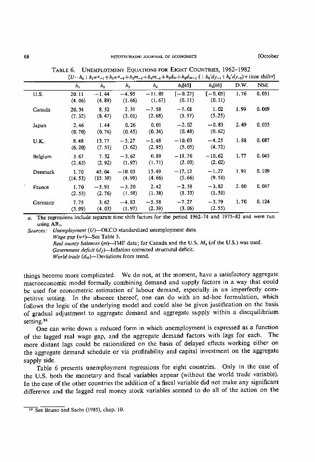
TABLE 6. UNEMPLOTMENY EQUATIONS FOR EIGHT COUNTRIES, 1962-1982 [ U= ho +hlwx_1 + h2wx_2 +h3m_1 +h4m_2 +h5dw +h6d w-1 (+hs'df-1 T h6'df-s) + time shifta]
hl
h2
h3
-4, 95 U,S. 20. 11 -1.44 (4. 06) (4, 89) (1 , 66)
8. S2 2, 31 Canada 20. 34 (7, 32) (8. 47) (3. O1)
O. 26 Japan 2. 46 1 . 44 (O. 70) (O. 76) (O. 45)
- 3. 27 U.K. 8. 48 13. 77 (6. 20) (7. 51) (3. 62)
-3. 62 7. 32 Belgium 3. 67 (2. 63) (2. 92) (1 . 97)
Denmark I . 70 45. 04 - 10. 03 (14. 53) (15. 38) (4, 99)
- 3. 20 -5. 91 France I , 70 (2. 53) (2. 76) (1 , 58)
-4, 83 3, 62 Germany 7 , 75 (3, 99) (4. 03) (1 . 97)
h4
h*[h5] h [h6] D.W. NSE [- O. 05] - 1 1 . 05 [- O. 27] I . 76
(1. 67) (O. 1 1) (O. 1 1)
-7. 58 -7. O1 1. OZ I . 99 (2. 68) (5. 57) (5. 25)
O. O1 -2. OZ -O. 83 2, 49 (O. 34) (O. 48) (O. 62)
- 1. 48 - 10. 03 -4. 25 l. 88 (2. 95) (5. 05) (4. 72)
O. 89 - 1 1. 76 - 10. 62 1 . 77 (1 . 71) (2. 03) (2. 02)
13. 49 - 17. 12 - I . 27 1 , 91 (4. 66) (5. 66) (9. 50)
2. 42 -2. 38 - 3. 82 2. OO (1. 38) (1 . 33) (1. 50)
-5. 58 -7. 27 - 3. 79 1 . 70 (2. 39) (3. 06) (2. 55)
C. 051
o. 069
o. 035
o. 087
o. 045
O. 100
C. 047
O. 124
a. The regressions include separate time shift factors for the period 1962-74 and 1975-82 and were run
using ARl' Sources: U,1employ,nent (U)-OECD standardized unemployment data.
Wage gap (wx)-See Table 5. Real money balances (m)-IMF data; for Canada and the U.S. M2 (of the U.S.) was used.
Government deficit (df)-Infiation corrected structural deficit.
World trade (dw)-Deviations from trend.
things become more complicated. We do not, at the moment, have a satisfactory aggregate
macroeconomic model formally combining demand and supply factors in a way that could
be used for econometric estimation of labour demand, especially in an imperfectly com-petitive setting. In the absence thereof, one can do with an ad-hoc formulation, which follows the logic of the underlying model and could also be given justification on the basis
of gradual adjustment to aggregate demand and aggregate supply within a disequilibrium
setting.10
One can write down a reduced form in which unemployment is expressed as a function
of the lagged real wage gap, and the aggregate demand factors with lags for each. The
more distant lags could be rationalized on the basis of delayed effects working either on
the aggregate demand schedule or via profitability and capital investment on the aggregate
supply side. Table 6 presents unemployment regressions for eight countries. Only in the case of
the U.S. both the monetary and fiscal variables appear (without the world trade variable).
In the case of the other countries the addition of a fiscal variable did not make any significant
difference and the lagged real money stock variables seemed to do all of the action on the
16 See Bruno and Sachs (1985), chap. lO.

1986] STAGFLATION IN THE INDUSTRIAL COUNTRIES : AN UPDATED OVERVIEW 69
domestic demand side. We note that the signs of coefficients are, in most cases, the "right"
Ones,17 although they are not always significant at the I percent level,
Because of the statistical problems that are attached to this type of single equation
estimation for each country, there is some advantage to also taking an overall cross-section
view of the rise in unemployment using the same underlying model. The following is the
resulting regression (20 years x 8 countries= 160 observations) of first differences:
AU=0.32+ 6.84 w'-1+7.47 Aw"-2- 5.75 Am-1+0.61 Am-2 (2)
(0.08) (2.30) (2.37) (1.08) (1.00) 9 56Ad~ 6 26Ad~_l
(1 .57) (1 .71) R2=0.51
With the exception of the second lag on money (which could be left out), all coefficients
have the right sign and are highly significant (numbers in brackets are standard errors of
coefficients). The assumption underlying (2), that the elasticities are the same across coun-
tries, is, of course, problematic, but it is reassuring to find such a strong overall qualitative
result. If one adds dummy variables for countries and/or each time period, none of these
dummies come out significant, and the overa]1 regression is not improved.
Table 7 gives a summary analysis of country regressions that were based on the adjusted
wage gap measure (these are not reported here). It indicates the role of the major factors
accounting for the increase in unemployment in each country. For each period the average
cumulative change in the average unemployment rate since 1965~9 is given, as well as the
TABLE 7. ACCOUNTING FOR THE RISE IN UNEMPOLYMENT SlNCE 1965-69 (Percentages of the labour force)
1970- 1974- 1978- 1970- 1978-1974-1982 1 974 1978 1982 1 974 1982 1 97 8
1982
Total
Adj. wage gap Aggregate demand
To tal
Adj, wage gap
Aggregate demand
Total
Adj. wage gap Aggregate demand
Total
Ad_i. wage gap
Aggregate demand
U.S. 3. 1.7 3.5
- O. -O. I O. 1 4. 1.5 3.2
Canada 4. 1.9 3.7 O.
O. 4 O. 1 4. 1.5 3.4
Ja pan
O. I O. 8 l. O. 3 O. 9 l.
-O. 2 -O. I -O. U.K.
O. 9 3. 1 6. O. 6 2. 5 3. O. 3 O. 8 2.
7 1 O
4 3 3
O 1 2
l 7 O
5. 8
o. o
5. 7
7. o
o. 4
6. 2
l. 1
l. 1
O. O
9. 5
5. 5
3. 9
o. 3
o. 7
- o. 2
O. 6
2. 5
-1.5
o. 7
- o. 2
o. 9
O. 2
O. 3
-O. 1
4. 3. 1.
8.
7.
- O.
2. o.
2.
2. l. 1.
Belgium
5 8. 1 10. 8 4 5. 6 12. 2
2. 3 - 1. 3 3
Denmark 8. 2 10. 2 O
8 Il. O 6. 3
-2. 4 4. 6 5
France
4. 8 5. 9 6
1.4 1.6 6
3. 3 4. 3 O
Germany 3. 3 5. 3 7
2 1.9 1.7
1.6 3.4 4
17 Only one of the 16 coefficients of the wage gap is significantly negative, for the case of the regresslon for France which is suspect anyway (see discussion below). Most of the coefficients on the demand variables
are negative as expected.

70 HITOTSUBASHI JOURNAL OF ECONOMICS [October estimated role of the adjusted wage gap (with its two lags) and the sum total of the aggregate
demand factors. The table reinforces the finding that wages played an important role mainly
in the mid-1970s and primarily for three of the European countries recorded (the U.K.,
Belgium and Denmark) and that its relative importance for most countries diminished during
the last sub-period, 1978-82, where most of the incrementa/ increase in unemployment can be
attributed to aggregate demand shifts (subtract the second column of Table 7 from the third
or fourth column). However, by 1982 the average remaining effect of the wage factor was
still high for the five European countries recorded in this table. Given what we know about
subsequent developments of the relevant variables, one may suggest that for most European
countries the further increase in unemployment after 1982 was mostly demand-induced.
V. The In ationary Process fi
There are various ways in which a price determination process can be described, which
is consistent with the theoretical discussion of supply and demand factors given in Section
III. Important elements in the inflationary process are changes in the variable costs, con-
sistlng of changes in nominal wages (vi,) and in the domestlc cost of materials (p~). If we
add another variable to take account of demand pressure (d) and assume that lagged in-flation also plays a role (on account of lagged adjustment or an adaptive expectation-for-
mation process) we can write down the rate of infiatlon (p) in the form
(3) p=ao + olw + a2 p~ + a3 p-1 + d,
where one assumes al+a2+a3=1. The negative intercept (ao) stands for autonomous shifts in productivity and capacity which mitigate the rate of infiation.
One may then append a wage-determination process to explain v~ and an equatlon for
exchange-rate formation (under fioating exchange rates) to account for the translation of
import prices from foreign (p*~) to domestic (p~=p**+~) import prices. Instead we here
100k at real wages and real exchange rates as given and rewrite the above equation as fol-
lows :
(3 ') p - p_1=ao + al(vi, - p_1) + (x2( p~ - p_D + d
When rewritten in this form the acceleration in inflation (p- p_1) is viewed as a function
of a real wage and a real import price rate of changel8 in addition to the previous demand
variable (d). For a measure of demand pressure we use relative deviations of GDP from capacity where the latter is crudely corrected for productivity and terms-of-trade changes
after 1973.19 For inflation the CPI change (p.) of respective countries is used, and for p*
the import deflator, as before.
Table 8 Iists regression results based on the above equation for the U.S.. Japan and
a pool of 8 EEC countries as well as large and small OECD country groupings. Japan's
18 Strictly speaking, IV -p_1 is not the change in the real wage but rather the excess of nominal wage growth
overpast infiation, which may or may not represent expected infiation. For an analogous equation including
instead thereal wage gap and leading to similar empirical results see Bruno and Sachs (1985), chap. 9. For an earlier application of a similar model after the first oil shock see Bruno (1980).
ID The trend growth rate from 1972 to 1978 was used as a reference measure of capacity after 1972,

1986] STAGFLATION lN THE IN'DUSTRIAL COUNTRIES : AN UPDATED OVERVIEW
TABLE 8. INFLATION ACCELERATION EQUATIONS, 1961-1980
Const. (1)
Real
wage (2)
O. 382 U.S. - O. 07 (O. 07) (O. 140)
O. 042 Japan - O. 43 (O. 87) (O. 097)
EECa O. 289 -O. 78
(O. 20) (O. 036)
7 Iarge O. 163 - O. 32
countriesb (O. 20) (O. 037)
12 small -O. 71 O. 269
countriesc (O. 17) (O. 030)
Real import Capacity
utilization
pr]ces (4) (3)
Statistics
R-2 D.W. p (5) (6) (7) O. 253 O. 77 O. 133
(O. 030) (O. 123)
O. 424 O. 56 O. 200
(O. 049) (O. 266)
O. 071 O. 60 O. 155
(O. 019) (O. 067)
O. 169 O. 57 O. 176
(O. 017) (O. 075)
O. 095 O. 52 O. 155
(O. 019) (O. 048)
2. O1 O. 735 (O. 244)
2. 17
2. 15
2. 20
2. 41
No. of obs. (8)
20
20
1 54
1 34
216
71
a. France, Germany, lialy (1967-80), U.K., Belgium, Denmark, Netherlands, Ireland.
b. Pooled regressions based on U.S., Canada, Japan, France, Germany, Italy, U.K. c. Australia, Austria, Belgium, Denmark, Finland, Ireland, Netherlands, New Zealand, Norway, Sweden,
Switzerland.
Source.' Based on IMF (IFS) data, as of 1981.
wage variable is insignificant and so is the capacity variable for EEC, but otherwise the
regressions are highly significant. One can show, in particular, the sizable contribution
of the import cost variable to both the acceleration of inflation during OPEC I and to some
extent also under OPEC Il (with the exception of Japan) and to the deceleration in the other
periods. Differences in import price behaviour, mainly on account of differential exchange
rate movements were particularly important in accounting for inter-country differences in
inflation profiles. When one reruns the regressions putting in foreign import prices (p**)
and real exchange rate movements (here measured by e' -p,-1) the resulting separate elas-
ticities for these two components are both almost identical to the one obtained for the com-
bined relative variable.20
When one leaves out the wage varlable and regresses the inflation rate itself on lagged
inflation, import prices and the capacity variable we get the following equation for the 7
large country group (again based on the period 1961-80) :
p=0.009 + O. 69 1 p_1 + O. 1 93 p* + 0.236d_1 (5)
(0.003) (0.039) (0.017) (0.073)
Equation (4) may be regarded as a reduced form in which wage adjustment is proxied
in part by capacity utilisation (which is negatively correlated with unemployment) and partly
by lagged inflation.
Given the different inflation deceleration profile of the U.S. and EEC after 1980 one
can ask whether it could indeed be predicted on the basis of a simple model like that of equa-
tion (4) if we knew in advance what the import prices (i,e., mainly differentiai exchange rate
*o For example, in the pooled 7 Iarge country regression, comparable to the one given in Table 8, the co-efficients are, respectively, 0,182 (with standard error 0.019) and O.161 (0.025) compared to the coefficient
of 0.172 (0.018) for the combined variable.

72 HITOTSUBASHI JOURNAL OF EcoNoivilcs [October movements) would be. Such an exercise produces the following estimates of inflation deceleration from 1980 to 1984 :
U.S.
Japan
EEC
Predicted
- 12. O
-5. O
- 5. 2
Actual
-9. 2
-5. 8
-6, o
The real depreciation of European currencies relative to the dollar (and to a lesser extent
also for Japan) thus explains why inflation slowed down so much less fast on the European
continent (in Japan inflation by 1980 had already come down much more than in the two
continents with wage moderation giving much of the explanation for that). It may also
help to explain why Europe as a whole was reluctant to expand and rather adopted con-
tractionary macro policies until very recently. These helped to support the slowdown but
at a formidable cost in terms of unemployment. The turn around in exchange rates that occurred during 1985 will, of course, alleviate some of this pressure.
VI. Problems of Policy Co-ordination
In the earlier sections we have seen the marked differences among the major partners
in responding to common exogenous shocks that have brought about world wide stagflation.
The U.S. has shown greater real wage flexibility after OPEC I but was slow in expanding
economic activity. Japan suffered a sharp reduction in output and productivity after OPEC
I but learnt from its mistakes and adjusted in an almost ideal textbook fashion when OPEC
II came around, suffering virtually no inflationary acceleration. In Europe some lessons
were learnt but only very slowly. The legacy of structural problems and relatively high
real wage costs has left a residue of "classical" elements in its mounting unemployment.
But as we have seen even the latter can only be explained as a results of highly contractionary
po]icies that were followed in Europe in the early 1980s while the U.S., in sharp contrast
to the post OPEC I revival, this time followed a highly expansionary fiscal policy. Both
this and the preceding discussion on the role of exchange rates in inflation lead us to a brief
discussion of the role of internal U.S. macro policy in world developments and the problem
of policy co-ordination among the major partners.
In Mundell's classic analysis of policy transmission between two countries, under fioat-
ing exchange rates and nominal wage rigidity in each, domestic monetary contraction and
domestic fiscal expansion are each likely to raise output and prices abroad. The channel
through which such policies are transmitted is the resulting rise in the domestic interest
rate which causes capital inflows and exchange rate appreciation domestically, implying
capital outflows and depreciation abroad. With complete nominal wage rigidity the for-
eign country gains in international competitiveness sufficiently to overcome any contrac-
tionary effects of higher interest rates, so that its output rises with the home country's. The
assumption of nominal wage rigidity in both countries turns out to be crucial for the above
outcome. Suppose, instead, that domestic wages are nominally rigid but the foreign country
has rigid real wages. In that case the resulting depreciation which raises the foreign coun-
try's import price may cause a wage-price spiral, and output contraction rather than ex-

1986] STAGFLATION IN THE IN'DUSTRIAL COUNTRJES : AN upDATED OVERVIEW 73
pansion may take place.21
Even if this argument wil] not hold by itself the unemployment result certainly holds
if the foreign country attempts to avoid the inflationary consequences by following con-
tractionary monetary or fiscal policy. Consider in this light the events of the early 1980s
when the U.S. (with relatively low wage indexation), simultaneously conducted contractionary
monetary policy and expansionary fiscal policy. This policy mix has caused the dollar to
appreciate and, as we have seen, helped to reduce U.S. inflation while Europe (with relatively
high wage indexation) was forced to import inflation (if not stagflation) from the United
States. To fight the inflationary consequences Europe had to conduct a contractionary
policy of its own thus exacerbating its bwn unemployment. Competitive monetary con-
tractions only drive up interest rates and raise unemployment, but the attempt to export
inflation to others may largely cancel out. The fact that macroeconomic policies in one
economy strongly affect policies in the other leads to situation in which decentralized policy-
making is likely to result in inefficient equilibria for the world as a whole.
The U.S. fiscal expansion in the years 1981-84 similarly explains its worsening current
account deficit, the improvement of Japan's current account balance and the appreciation
of the dollar relative to the yen since 1980 [see Ishii, McKibbin and Sachs (1985)]. While
it is generally agreed that the only way to bring down real interest rates and reverse the dollar
appreciation trend in any sustained fashion is by the U.S. following a contractionary fiscal
policy, there is less agreement on the mix of policies that should be followed by its major
partners. It would seem that an optimal world outcome should dictate a more expansionary
fiscal and monetary policy in both Japan and Europe along with the fiscal contraction of
the U.S. The argument hinges, in the case of Japan, on the inflationary and exchange rate
consequences of a fiscal expansion on its part. If it is correct that the financial liberalization
has greatly increased the substitutability of domestic and foreign assets then fiscal expansion,
in a true Mundellian fashion, should appreciate rather than depreciate the yen and worsen
rather than further improve its current account. Thus fiscal expansion in Japan would be positively transmitted and help to alleviate contractionary effects in the rest of the world
while at the same time it would not necessarily be inflationary at home.
THE MAURICE FALK INSTITUTE FOR ECONOMIC RESEARCH IN ISRAEL
REFERENCES
Artus, J. A. (1984), "The Disequilibrium Real Wage Hypothesis: An Empirical Evaluation,"
IMF StaffPapers, 31 (no. 2, June 1984), pp. 249-302.
Bruno, M. (1980), "Import Prices and Stagflation in the Industrial Countries: A Cross Sec-
tron Analysis," Economic Journal, 90 (359), (Sep.), pp. 479~92.
Bruno, M. (1985), "Aggregate Supply and Demand Factors in OECD Unemployment: An Update," Jerusalem: Falk Institute Discussion Paper no. 85.10, (August).
Bruno, M, and J. Sachs (1985), Economics of Worldwide Stagflation. Harvard University
Press.
21 For a detailed analysis see Bruno and Sachs (1985), chap. 6.
74 HrroTSUBASHI JOURNAL OF ECONOMICS Gordon, R. J. (1977), "World Inflation and Monetary Accomodation in Eight Countries,"
Brookings Papers on Economic Activity, 2, pp. 409-468.
Hamada, K., and M. Sakurai (1978), "International Transmission of Stagflation under Fixed
and Flexible Exchange Rates," Journa/ of Politica! Economy, (October), pp. 877-896.
Ishii, N., W. McKibbin, and J. Sachs (1985), "Macroeconomic Interdependence of Japan
and the United States: Some Simulation Results," NBER Working Paper 1637, Cam-bridge, Mass. (June).
Layard, R. and S. Nickell (1984), "Unemployment and Real Wages in Europe, Japan and the U.S,," Centre for Labour Economics, LSE, Working Paper 677, (October).
Lipschitz. L., and S. M. Schadler (1984), "Relative Prices, Real Wages and Macroeconomic
Policies : Some Evidence from Manufacturing in Japan and the U.K.," IMF Staff Papers,
31, No. 2, (June), pp. 303-338.
Newell, A., and J. S. V. Symons (1985), "Wages and Employment in OECD Countries," Centre for Labour Economics, LSE, Discussion Paper 219, (May).
Sachs, J. (1979), "Wages, Profits and Macroeconomic Adjustment: A Comparative Study,"
Brookings Papers on Economic Activity, 1979 (2), pp. 269-319.
Shinkai, Y. (1980), "Oil Crises and the Stagflation (or its absence) in Japan," Institute of
Social and Economic Research Discussion Paper 1 10, Osaka University, (November).


